Comparative Study on Michigan Solar Photovoltaic Promotion Policies

---- Governmental Expenditure Efficiency Optimization

By

Shiming Yang

A practicum submitted in partial fulfillment of the requirements

for the degree of Master of Science of Environmental Policy and Planning

(Natural Resources and Environment) At the University of Michigan

December, 2013

Faculty Advisor: Professor Shelie Miller

ABSTRACT

State of Michigan has relatively little solar resources but substantial installation capacity. Three governmental promotional policies are currently in position or have high potential to be adopted by the state government. This study analyzes three policy options: property tax exemption, Feed-in Tariffs, and Green Power Purchase. This study uses the optimization model to analyze governmental expenditure cost-efficiency of three major incentive schemes in Michigan. Realistic variables are incorporated into the model, including degression rates, discount rates, cumulative installation capacity, and economy of scale. This study constructs a handy framework where the cost-efficiency of governmental promotion policies could be measured and compared, with the purpose to assist state and local governments in making renewable energy policies with limited information.

INTRODUCTION

Humans are facing energy challenges. Climate change and the exhausting fossil-fuel sources are pushing us to explore reliable low-carbon and renewable energy sources. Solar power is one renewable energy source that is getting most attention in the U.S. and abroad. It is almost universally distributed, inexhaustible, and low carbon emission. The U.S. solar photovoltaic (PV) power, under governmental support, has been growing in scale and complexity. Due to the high energy-generation cost, in no state has solar PV electricity reached grid parity, which necessitates further governmental support. The U.S. Government has a variety of support schemes available for solar PV industry, including R&D and market support. Compared with R&D that usually takes more time with uncertain results, market support has a direct impact on solar PV development. There have been several government support schemes in the U.S., including tax incentives, Feed-in-Tariffs (FITs) and Net-Metering programs, Renewable Portfolio Standards (RPSs) and Renewable Energy Certificates (RECs), tendering scheme of some sort, and the loan scheme.

Solar PV Energy in Michigan

The State of Michigan is a Midwest State with a slowly declining population from 2000 to 2010, a higher poverty rate and lower per-capita income than national average1. Michigan’s unemployment rate is higher than national average since 20032. According to NREL, Michigan’s solar resource ranges between 4-4.5 kWh/m2/day,3 ranking among the lowest group in the U.S. states. Although known more for wind resources, Michigan has great potential for economically feasible solar energy. Moreover, the solar resource of

a state does not alone determine solar PV installation area, as financial incentives play an important, if not the dominant, role. “As of the end of 2009, according to the Energy Systems Bureau of Michigan, the state had 1,041 kilowatts' worth of installed solar photovoltaic systems, but its economically feasible solar potential is much greater -- estimated at more than 2,350 megawatts.”4 Michigan’s solar PV installation area ranks 25 (7.10MW), much higher than its radiation ranking.5 Considering other states with low solar radiation and high installation area, such as Vermont, New York, and Pennsylvania, Michigan has a great prospect in PV installation.

Solar Photovoltaic Power in Michigan took off after 2000 and the installation capacity has reached 7.10MW by 2013, with an average growth rate of 25% between 2003 and 20106. Michigan’s solar PV installation is dominated by residential installations, with 88% of total installations (count) are below 25kW, and 45% of total counts are 4kW or smaller in size. Installations larger than 25kw are very limited7. Given that Solar PV energy has not reached grid parity by far, adoption of solar PV depends largely on governmental support that provides compensation for at least one participant group’s financial sacrifices—manufacturer, distributor, or customer8. Michigan governmental support to Solar PV sales market well orchestrates those of national policies.

Michigan Government Support Schemes

Michigan state government has been supporting distributed solar PV development with a variety of policies, including tax incentives, RPS Renewable Energy Credits (RECs), and net-metering programs. Utilities have voluntarily launched experimental Feed-in Tariffs (FITs).

The Clean, Renewable and Efficient Energy Act of 2008 established in Michigan a RPS that requires Michigan electric providers to achieve a retail supply portfolio which includes at least 10% renewable energy by 2015, with additional targets for the two major electricity providers in Michigan: DTE Energy and Consumers Energy. Unsuccessful attempts were made in 2012 to raise the RPS to 25% by 2025. Corresponding REC requirements are prompting electricity providers to launch incentive programs, such as SolarCurrents Program by DTE Energy in 2009. This program offers a $0.11 per kWh for the duration of a 20-year contract, in exchange for RECs produced by the system.

In terms of tax incentives, Michigan has property tax exemption for commercial and industrial sectors and isn’t currently functioning due to an interpretation difference between the legislative and implementing bodies9. According to Michigan property tax assessment that includes the replacement costs of the system, property tax burden is

estimated to be $0.06/kWh - $0.084/kWh. In the fiscal year of 2008-2009, 287kW of solar PV was installed, which translates to $27,638 revenue loss, should all PV installations be exempt. This potential loss constitutes only 0.00276% of approximately $10 billion total property tax expenditures.10

Michigan also has mandatory net-metering programs and experimental FITs program for Solar PV energy. Under the statewide net-metering program, PV systems qualify for true net-metering where net excess generation is carried over to the next billing cycle at the full or partial retail rate, depending on the system size.11 Systems below 20kW get full retail rates, while systems from 20kW-150kW qualify for a portion of retail rates. Consumers Energy began the Experimental Advanced Renewable Energy Program (EARP) in 2009. This program enables residential systems below 20kW and non-residential systems below 150kW to get between $0.2/kWh and $0.259/kWh, with 15-year contracts.

Distributed solar PV systems have multiple advantages over utility-scale systems in Michigan. Utility scale solar PV systems require big upfront investment and burdens ratepayers with costly electricity. Utility-scale systems also demand large areas to install, while the majority of Michigan land is forested. Distributed solar PV installations have advantages over utility-scale solar on both aspects. Distributed systems save land area, reduce upfront investment, disperse value among a mass of stakeholders, maximize social and ecological benefit, and usually save heat/cooling/shading costs of a building. Therefore, distributed solar installations, when have governmental support, have apparent advantages over utility-scale solar PV farms. That partly accounts for the fact that Michigan has more distributed solar PV than utility-scale solar farms. Considering these advantages, the state government of Michigan has initiated the net-metering and experimental FITs programs, as mentioned above, to test residential customers’ acceptance to rooftop solar. Shortly after these programs launched the enrollment was full.

Statement of Need and Goal

This study attempts to construct a handy framework where the cost-efficiency of governmental promotion policies could be measured and compared. This study analyzes cost-efficiency of three major incentive schemes in Michigan, which are also widely applied in U.S., aiming to find out factors that influence subsidy efficiency, in order to compare various subsidy scheme’s desirability under certain conditions.

This research aims to optimize the solar PV system customer-utility-government cooperation that maximizes expenditure efficiency, i.e. to boost installation area with smallest expenditure. The research starts with a review of status quo and potential of distributed solar PV in Michigan, including current installation size, governmental incentives, and economic parameters that influence solar PV industry. The study builds a system that includes three actors: customers, utility, and the state government. The optimization model composes of objective (minimize governmental budget to reach certain RPS target), decision variables (individual system size, system price), and constraints. We assume there is an optimum arrangement of governmental funding to reach a specific RPS solar PV target. The main customer groups studied here include residential as well as commercial and industrial solar PV installers.

We analyze three policy options in this research: Property tax exemption; Governmental Feed-in-Tariffs; and Green Power purchase. These three policies have either been in place or in experimental stage in Michigan. In other words, they are most-probable policies of Michigan government. Although there are currently no functioning property tax exemptions for residential, commercial, or industrial installers, it is a high-potential policy option for its wide application in other states, low governmental expenditure, and little barriers compared to other policies. The experimental FIT program (EARP) is under practice by Consumers Energy. It is highly probable that Michigan government will consider a governmental FIT program, depending on EARP’s result. Michigan government has purchased green power in Ann Arbor and Lansing, implying an upscaling potential if financially feasible.

LITERATURE REVIEW

Scientists have studied tax incentives, Feed-in-Tariffs, and Green Power Purchase and their application in the U.S. and abroad. Because the United States has a relatively short enforcement history of the three policies and on limited scales, most literature studies EU counterpart policies.

A diversity of tax incentives exist in EU-27 countries to promote green electricity, primarily by means of exemption from electricity-related taxes. The three kinds of direct tax incentives concern personal income tax, corporate tax, and property tax. Effective property tax incentives have been established in Spain and Italy, both of which are borne by municipalities. The property tax incentive in Spain targets specifically solar energy

systems and includes a bonus of up to 50% of the full share of the tax on real estate, based on a municipal optional bonus12.

Having been practiced in Europe with visible success in Solar PV penetration, FITs has a promise in the U.S. to facilitate solar PV development when designed appropriately, as have been attempted by Lesser and Su.13 A research on willingness-to-pay of American customers suggests that American consumers are willing to pay 1.5% to 10% more on electricity to support renewable electricity.14 A research surveys the six state-level policies that have FIT design features.15 This study pointed out that FITs in the U.S. focuses more on distributed and specific renewable energy, therefore in a less-competitive but more complementary position with RPS than its European counterparts. Green Power Purchase as a policy option and has not been widely studied. This policy instrument is usually used as a policy instrument to reach renewable energy targets.

Andy Walker’s Renewable Energy Planning: Multi-parametric cost optimization provides an analytical framework to proceed the study.16 This study aims to find a cheapest combination of renewable energy technologies (lowest life-cycle cost), with a specified goal regarding percent of energy use from renewable sources, such like RPS. Cost-efficiency is calculated on three parameter groups: Renewable energy sources and their associated costs; State, utility, and federal incentives; and economic parameters (discount rate, technology advance). The study considered solar thermal, solar PV, biomass, wind, and other renewable energies as compared to the current energy portfolio. The analysis is performed by MS Excel Spreadsheet (“Premium Solver”) that would use to calculate for an optimization model. The solver routine calculates the change in life-cycle cost associated with a change in the size of each of the renewable energy technologies, and then moves in the direction of decreasing life-cycle cost by an amount determined by a quadratic approximation.

Financial Analysis of Residential PV and Solar Water Heating System in the US provides an economic analysis of payback period, net present value, and internal rate of return, on residential solar PV and thermal systems in Michigan and Hawaii.17 The study aims to find the financial feasibility of solar PV and thermal systems without governmental support, while introducing “one of the most powerful trends in their favor: the rising cost of fossil fuels” as the major independent variable driving the financial attractiveness of solar energy systems. The study chooses Michigan and Hawaii, two states with contrasted solar isolation, conventional utility rates, and governmental incentives on renewable energy. The study concludes that residential PV systems are not currently economically attractive in Michigan under any likely assumptions, while higher utility rates and solar radiation in Hawaii makes it a reasonable investment without governmental subsidies.

The study is not an examination of distributed solar PV’s financial viability from a property owner’s perspective. Instead it considers government’s expenditure. Owing to the nature of renewable energy penetration that could vary significantly with investors’ perception and expectation, policy effect might deviate from that of financial analysis. Current experience and data availability necessitates the state government to make promotional policies with imperfect information, so it is useful to find the best policy under limited information and budget, as in this study.

RESEARCH METHODS

The system we study consists of four players: Federal and Michigan state government; Solar PV manufacturers, Solar PV system owners in Michigan (residential and commercial); and utilities that provide electricity for Michigan state (such as DTE Energy and Consumers Energy Company). This study divides interactions among the four players through two subsystems: the Government-Customer-Manufacturer model (subsystem-1), and the Government-Customer-Utility model (subsystem-2). Due to solar PV module price volatility and unavailable data, the system focuses more on subsystem-2, the electricity market.

There are currently no property tax incentives for household and business solar PV customers at work, but as a policy option, we will include it in the model. Most state governments support solar PV mainly through gross-metering (FITs) and net-metering programs. Although Michigan state government has not made its FITs plan, Consumers Energy’s EARP might influence government decision making on the issue, so we

consider it as a viable policy option. Another policy option considered is Green Power Purchasing, which was already launched in three major cities in Michigan.

The study sets an approximate context from Michigan Proposal 3, and draw data from NREL, DOE, EIA, and other public-available database. We set the goal based on Michigan Proposal 3, or the “25X25” proposal, which proposes to “require electric utilities to provide at least 25% of their annual retail sales of electricity from renewable energy sources, which are wind, solar, biomass, and hydropower, by 2025”.18 Michigan electricity generation in 2010 is 26,356MW.19 In the current RES that sets a 10% goal by 2015, wind power makes up for 94% of renewable energy, and solar only 2%. To give reasonable space for solar PV growth based on its potential, we set the goal to be “2% of renewable energy generated under Proposal 3 is solar PV by 2025”. Given Michigan solar PV installation by 2012 is 7.09MW, the solar PV gap to be filled is then 26,356*25%*2% - 7.09=124.7MW.

We compare three policy options in reaching the RPS target. For each option, we set up a model to optimize each objective. We set the policy activation years from 2015 to 2025, a period of ten years.

Option 1: Property tax exemption to PV system owners;

Option 2: Feed-in Tariff to PV system owners;

Option 3: Green Power Purchase from utilities

An optimization model consists of a well-defined system, objective(s), variable(s), and constraints. We use the optimization model to find the cost-efficient policy for two reasons. Renewable energy penetration depends largely on financial feasibility, which relates to subsidy and installation cost. Energy cost of solar photovoltaic and fossil fuel energy both change with time and system sizes, which in turn might change with cumulative capacity installed. 20 An optimization model accommodates these inter-connected variables in a single system to find a best solution. It is also adaptive to new variables, which means we can improve the model accuracy by putting in new information without undoing the whole system. A simplified model for this study is as below.

Objective: minimize total governmental spending

= S1+S2+S3 +…+S10

Variables: S1, S2,….S10 (Sn=installation area in year-n)

Constraint: S1+…..+ S10= Stotal

Other constraints differ among each scenario.

DATA AND RESULTS

There are three groups of data to be collected: costs of solar PV energy; governmental incentives; and economic parameters. The costs of solar PV energy includes output cost of solar PV installations and cost of conventional energy. Since we do not study the financial viability for customers or collective social benefit, we do not consider the decreasing unit output cost with increasing system-size for solar PV systems.

Michigan average solar radiation is 4.2 Peak Sun Hours. Therefore the annual output (kWh) is:

Output= 4.2*S*24*365=S*3.68*104

Scenario 1 Property Tax Exemption

The property tax burden for small-size systems ranges from $0.06/kWh to $0.083/kWh, take Lansing’s example.21 In terms of payment level, property tax exemption alone is not a sufficient financial incentive for customers to purchase solar PV systems. Although 36 states have offered property tax incentives, and in some states solar PV installations increased quickly under promoting policies that includes property tax exemption, it is impossible to directly tie tax treatment or exemptions to the increase in installations.22 However, we can still calculate potential governmental tax revenue loss, if property tax exemption was able to stimulate the energy target set in this study.

Potential tax revenue loss: 124.7* 103*3.68*104/106 =385.5 million $

Scenario 2 Feed-in Tariff

The EARP Program, due to its experimental nature and small size, has a simple design. The program has a size limit of 2,000kW. 500kW is reserved for residential systems with installations from 1kW to 20kW. 1,500kW is reserved for commercial systems from 20kW to 150kW. There are two time phases for installation, meaning that early installers get higher tariffs. The contract period is up to 12 years.

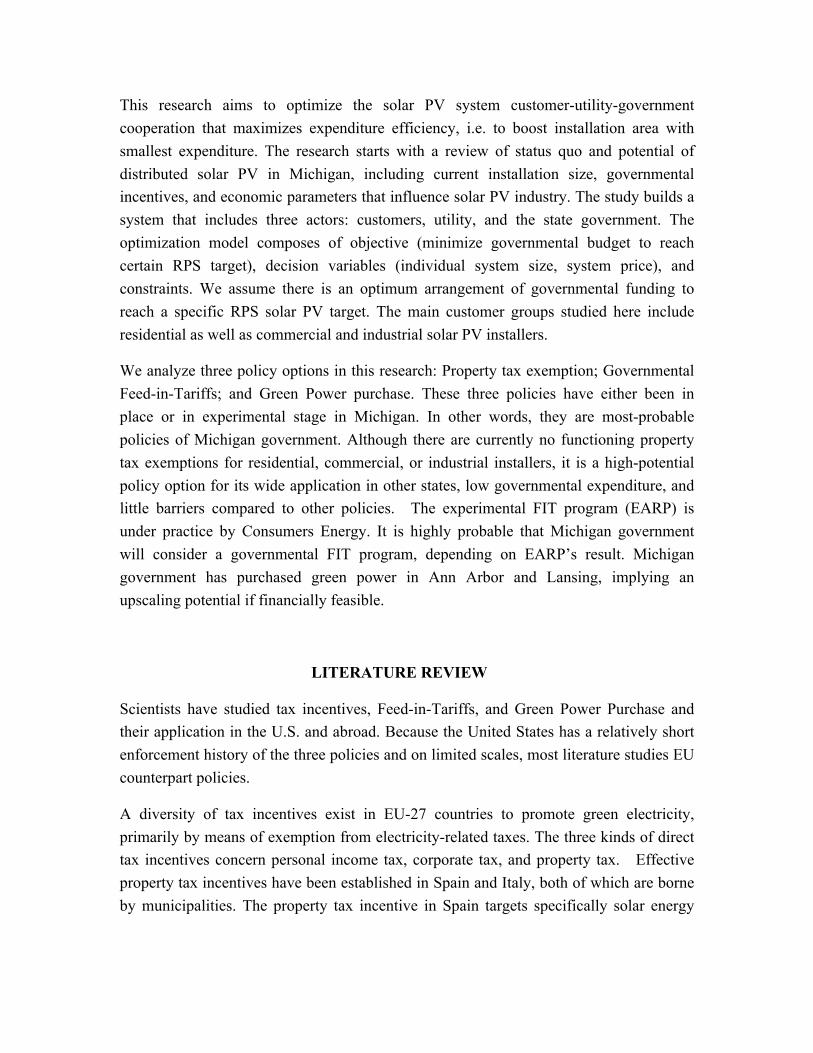
Table 1 Customer Class 1st Phase 2nd Phase

Residential 0.65$/kWh 200kW 0.525$/kWh 301kW Commercial 0.45$/kWh 833kW 0.375$/kWh 687kW

A closer look at the EARP program design helps us build the scenario (Table 1). The program is in accordance with NREL’s guidebook on solar PV FIT design. There are two kinds of FIT payment structure: the premium-price FIT, and the fix-price FIT. Majority of countries are adopting the fix-price FIT, so does the EARP. Fix-price FIT disconnects FIT payment with market price, thus largely reducing investment risks in solar PV market. The EARP differentiates payment level by system size. Differentiating “FIT payments by project size helps a jurisdiction capture the benefits of both large and small-scale deployment”, although too high payments to small systems might increase cost of the policy. For this reason, the lowest payment level is typically offered to the largest systems, while the capacity for different size range is predetermined (in EARP, ¼ of program capacity is reserved for residential sizes, and ¾ for commercial sizes). The program also differentiates systems installed at different times through tariff degression to encourage program enrollment, but also might have assuming that installation costs decreases over time. Because solar PV installation costs have been decreasing continually in years, the corresponding FIT ought to also decrease.

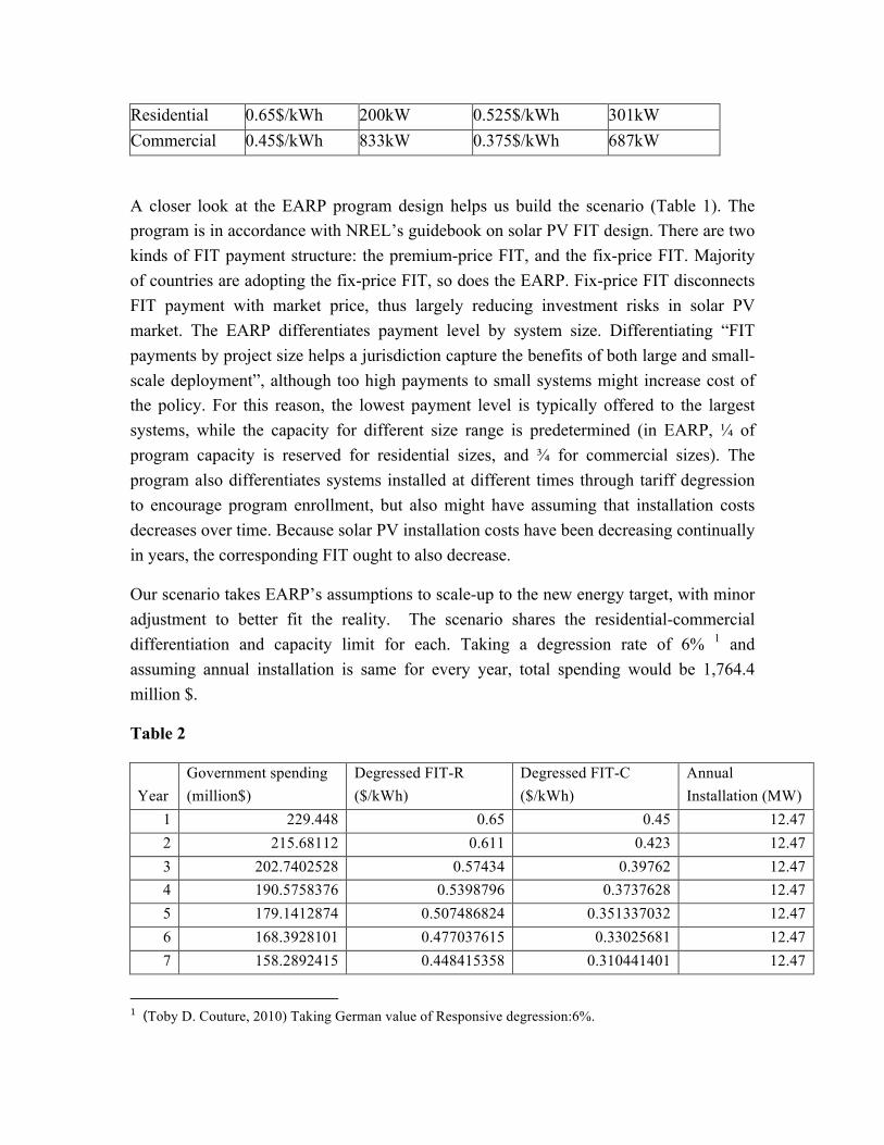
Our scenario takes EARP’s assumptions to scale-up to the new energy target, with minor adjustment to better fit the reality. The scenario shares the residential-commercial differentiation and capacity limit for each. Taking a degression rate of 6% 1 and assuming annual installation is same for every year, total spending would be 1,764.4 million $.

Table 2

Year Government spending (million$)

Degressed FIT-R ($/kWh)

Degressed FIT-C ($/kWh)

Annual Installation (MW)

1 229.448 0.65 0.45 12.47 2 215.68112 0.611 0.423 12.47 3 202.7402528 0.57434 0.39762 12.47 4 190.5758376 0.5398796 0.3737628 12.47 5 179.1412874 0.507486824 0.351337032 12.47 6 168.3928101 0.477037615 0.33025681 12.47 7 158.2892415 0.448415358 0.310441401 12.47

1 (Toby D. Couture, 2010) Taking German value of Responsive degression:6%.

8 148.791887 0.421510436 0.291814917 12.47 9 139.8643738 0.39621981 0.274306022 12.47

10 131.4725114 0.372446621 0.257847661 12.47 Total 1764.397322 124.7

However, the scenario relates cumulative installation with tariff degression rate, because “tariff degression based on capacity installed will be more likely to keep up with rapidly changing market conditions.”23 Owing to lack of data and practice, this paper makes an estimate by finding the relation between a fixed tariff degression rate and linear installation accumulation (same annual capacity increase). We assume that when cumulative installation area increases linearly, the annual degression rate is fixed. We use the Excel spreadsheet solver to minimize governmental spending for a total of ten years.

Sr-n= residential installation (kW) in year n Sc-n=commercial installation (kW) in year n Stotal-n=total installation (kW) in year n Q=output ($) Cgov-n= governmental spending (million $) in year n Scum-n=cumulative installation (kW) at beginning of year n FITr-n =Feed-in Tariff ($/kWh) for residential systems in year n FITc-n=Feed-in Tariff ($/kWh) for commercial systems in year n Objective: to minimize C=Cgov-1+Cgov-2+…+Cgov-10

Constraints: 3Sr-n=Sc-n

Sr-n+Sc-n=Stotal-n

Stotal-1+Stotal-2+…+Stotal-10 =124.7

FITr-n=6E-06*(Scum-n)2-0.0031Scum-n+0.6495

FITc-n=4E-06*(Scum-n)2-0.0022Scum-n+0.4497

Q= S*3.68*104*10-6=S*3.68*10-2

Cgov-n= Q*Sr-n*FITr-n + Q*Sc-n*FITc-n

Sr-n, Sc-n, FITr-n, FITc-n, Q,Cgov-n >=0

Variables were aligned in Table 2. Annual governmental spending is calculated from residential/commercial installations and annual degressed FIT levels in each year. Minimized total governmental spending is 1,759.7 million$. as compared to 1,764.4 million $ when annual installation quota was allocated evenly along the 10 years. There is a 4.7 million USD governmental saving through optimization.

Table 3

Year

Government spending (million$)

Degressed FIT-R ($/kWh)

Degressed FIT-C ($/kWh)

Annual Installation (MW)

Cumulative installation (MW)

1 200.7159279 0.65 0.45 10.90847434 0 2 196.805531 0.616397698 0.426177336 11.28902327 10.90847434 3 190.3792615 0.583644131 0.402836421 11.54666675 22.19749761 4 184.1256587 0.551725102 0.380017513 11.82995807 33.74416436 5 178.0621028 0.520682224 0.357744933 12.14277538 45.57412243 6 172.2250487 0.490565059 0.336047786 12.4908313 57.71689781 7 166.6691832 0.461430791 0.314959497 12.88209912 70.2077291 8 161.4673088 0.43334505 0.294518056 13.3273634 83.08982823 9 156.712058 0.406384355 0.274767278 13.84099335 96.41719162

10 152.5179406 0.380640831 0.255759462 14.44181503 110.258185 Total 1759.680021 124.7 124.7

In order to examine the sensitivity of total spending to annual degression rate, a starting degression rate of 5%, 7%, and 8% were plugged in. Result shows that total spending and starting degression rate are approximately linear related, as shown in the figure below.

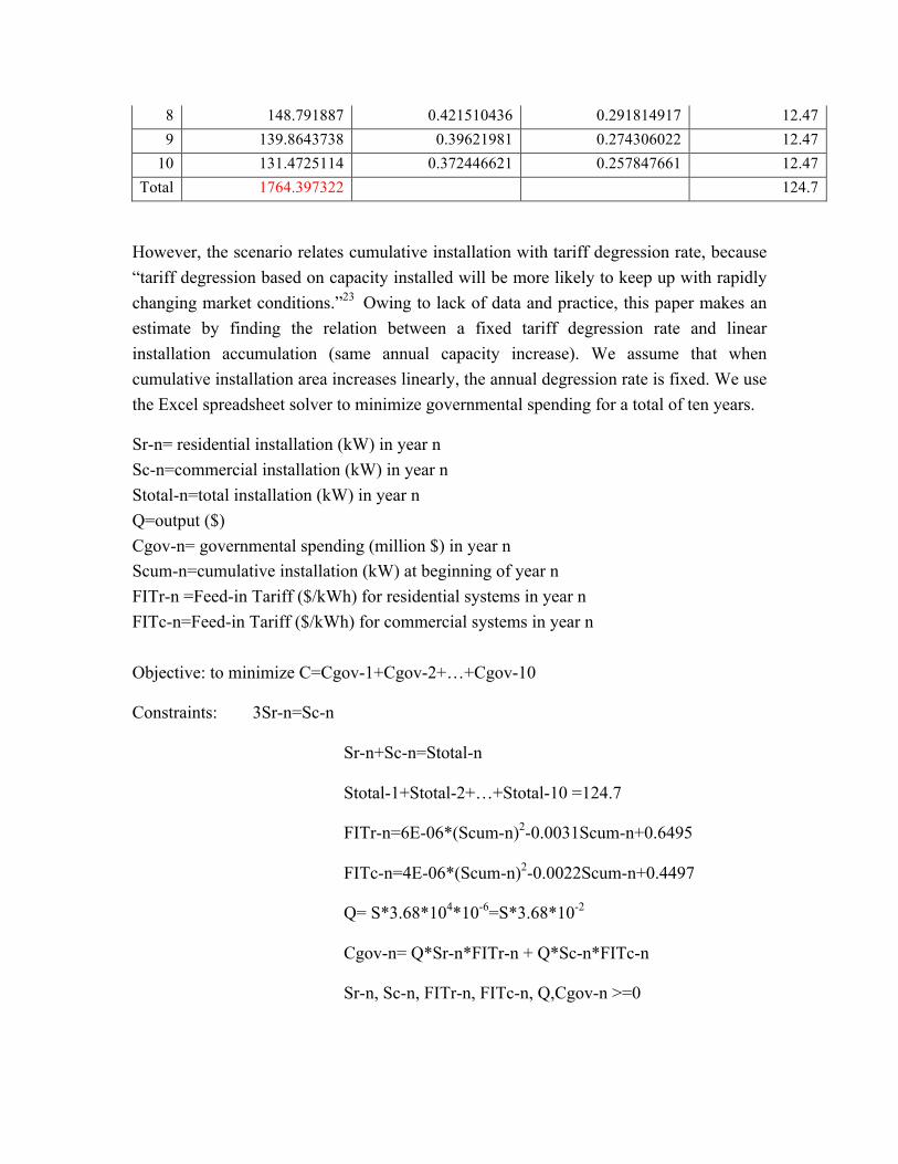
Optimization Result changes when the discounting rate is considered. The discount rate is defined as an interest rate used to bring future values into the present when considering the time value of money.24 Assuming governmental spending in this study applies a discount rate of 5%. The optimization result with the discount rate considered is shown in table 3.

Table 4

Year

Government spending (million$)

Degressed FIT-R ($/kWh)

Degressed FIT-C ($/kWh)

Annual Installation (MW)

Cumulative installation (MW)

Discounted 5%

1 3.6194E-11 0.65 0.45 1.96706E-12 0 3.6194E-11 2 0 0.6495 0.4497 0 1.96706E-12 0 3 0 0.6495 0.4497 0 1.96706E-12 0 4 0 0.6495 0.4497 0 1.96706E-12 0 5 53.97060841 0.6495 0.4497 2.935239907 1.96706E-12 43.95939786 6 170.1765798 0.64045245 0.443276935 9.38822085 2.935239907 131.6793935 7 279.6398367 0.612208478 0.423195857 16.15245948 12.32346076 205.5609763 8 373.8815296 0.566089915 0.390296488 23.39653378 28.47592024 261.0954164 9 447.552697 0.504839901 0.346343607 31.50978354 51.87245401 296.9156033

10 499.8391222 0.432730649 0.294069468 41.31776245 83.38223755 315.0233117 Total 1825.060374 124.7 124.7 1254.234099

Scenario 3 Green Power Purchase

Green power purchase is another promotional policy used in sixteen U.S. states. Michigan currently has three Green Power Purchase programs to reduce carbon emission and foster renewable energy penetration. The green power purchase policy is usually accompanied with energy efficiency and saving initiatives. By an executive order from the Mayor’s office, the city of Lansing has required to procure 10% of their energy consumption from renewable sources by 2010, escalating to 15% in 2015 and 20% in 2020.25 The city of Ann Arbor adopted a resolution in 2006 that established a goal of 30% renewable energy for all municipal operations by 2010, and 20% renewable energy for the entire Ann Arbor community by 2015.26 The city of Grand Rapids in 2005 established a goal of purchasing 20% of its municipal power demand from renewable energy by 2008. It also purchased renewable energy from Consumers Energy that equals roughly 15% of municipal electricity consumption. The Mayor has also established a further goal of purchasing 100% of the city's municipal electricity consumption from renewable energy by 2020.27

Although Green Power Purchase has not been financially attractive, it has a good potential to be in future, considering the annually rising conventional energy and the decreasing solar energy cost. In this scenario, we make a rough optimization model that minimizes net governmental spending (or saving) on solar PV power purchase, given the energy target over ten years.

Average retail price of electricity to ultimate customers in Michigan is 0.104$/kWh in 201128. This is the starting utility rate in Year-1. Michigan electricity rate 1990-2011 has increased from 0.078 to 0.133$/kWh, a 2.70% increase annually. So we assume the conventional energy price increases 2.70% annually. Solar PV cost degression rate equals FIT degression rate in Scenario 2, which is 6%. We assume that local government purchases energy from systems of capacity greater than 25kW (non-residential systems), the solar PV unit cost of which is 6.891$/W.29

Sn=total installation (MW) in year n Qn=total annual output (MWh) in year n Cs-n=total cost of solar purchase (million $) in year n Cu-n= total cost of utility purchase (million $) in year n, for the amount of solar purchase (kWh) Cgov-n= governmental spending (million $) in year n Dn=solar PV cost degression rate (%) Du-n= utility cost increasing rate (%) Pn= utility rate for year n ($/kWh) Objective: to minimize C=Cgov-1+Cgov-2+…+Cgov-10

Constraints: Stotal-1+Stotal-2+…+Stotal-10 =124.7

Cgov-n= Cs-n - Cu-n

Cs-n=Sn*106*6.891/10 6 *Dn(n-1) =6.891*Sn* Dn(n-1)

Pn=0.104* (1+2.7%)(n-1)

Cu-n=Qn*Pn*103/106

Table 5 shows the net government spending before optimization, with an even distribution of solar installations over ten years. Table 4 shows the optimization result, showing that all capacity should be installed in year-10 (the last year) when utility energy cost is highest while solar PV energy cost lowest. With optimization result, local government has a cumulative saving of 723.6 million USD.

Table 5

Year

Net Government Spending (million $)

Annual solar installations (MW)

Annual solar output (MWh)

Annual total cost of solar purchase (million $)

Utility rate ($/kWh)

Total utility cost replaced (million $)

Solar PV cost degression rate

1 38.193116 12.47 458896 85.9183 0.104 47.725184 1

2 36.90453603 12.47 458896 85.9183 0.106808 49.01376397 0.94

3 34.22206174 12.47 458896 85.9183 0.112653495 51.69623826 0.8836

4 29.92058923 12.47 458896 85.9183 0.122027019 55.99771077 0.830584

5 23.62346391 12.47 458896 85.9183 0.135749355 62.29483609 0.78074896

6 14.74710377 12.47 458896 85.9183 0.155092213 71.17119623 0.73390402

7 2.410522194 12.47 458896 85.9183 0.181975388 83.50777781 0.68986978

8 -14.70997598 12.47 458896 85.9183 0.219283402 100.628276 0.64847759

9 -38.61445069 12.47 458896 85.9183 0.27137467 124.5327507 0.60956894

10 -72.35861374 12.47 458896 85.9183 0.344908027 158.2769137 0.5729948 Total 54.33835247 124.7

Table 6

Year

Net Government Spending (million $)

Annual solar installations (MW)

Annual solar output (MWh)

Annual total cost of solar purchase (million $)

Utility rate ($/kWh)

Total utility cost replaced (million $)

Solar cost degresses with time

1 0 0 0 0 0.104 0 1 2 0 0 0 0 0.106808 0 0.94 3 0 0 0 0 0.112653495 0 0.8836 4 0 0 0 0 0.122027019 0 0.830584 5 0 0 0 0 0.135749355 0 0.78074896 6 0 0 0 0 0.155092213 0 0.73390402 7 0 0 0 0 0.181975388 0 0.68986978 8 0 0 0 0 0.219283402 0 0.64847759 9 0 0 0 0 0.27137467 0 0.60956894

10 -723.5861374 124.7 4588960 859.183 0.344908027 1582.76

9137 0.5729948 Total -723.5861374 124.7

DISCUSSION AND CONCLUSION

For comparison convenience, we set base cases for the FIT and Green Power Purchase options. In the base cases, degression rates is fixed to 6%, and total installation area increases by same amount every year till the RPS target is reached. No discount rate is considered in the base cases.

In order to reach solar PV energy target of 124.7MW within ten years, the property tax exemption policy costs 385.5 million USD, although it is not guaranteed this policy alone will meet the 124.7MW target.

In the FIT scenario, the total spending of the base case is 1,764.4 million USD. We then relates degression rate with cumulative installation area and optimize through Solver. The minimized total spending reduces to 1759.7 million USD. Optimization reduces total spending by 4.7 million USD. If we consider discount effect, however, the minimized total spending increases to 1,825 million USD, and the allocation of yearly installation changes.

In the Green Power Purchase option we calculate the “net total spending” by subtracting replaced conventional electricity from total spending on solar PV electricity purchase. In the base case, the total net spending is 54.4 million USD. After optimization, the government would purchase all of 124.7 MW in year ten, when conventional utility price peaks and solar PV unit cost reduces to the lowest. The total net spending is -723.6 million USD, implying a net saving of 723.6 million USD. The result does not change when at a discount rate of 5%.

By comparison, the optimized Scenario 3 has the smallest total spending. Optimized Scenario 2 with discount rate is the least cost-efficient option. Among the three scenarios, Scenario 1’s financial attractiveness to customers is not tested, while the FIT and Green Power Purchase scenarios provide net profit for customers.

Policy Instrument Total Net Spending (million USD)

Green Power Purchase Optimized -723.6 Green Power Purchase Base Case 54.4 Property Tax Exemption 385.5

Feed-in Tariff Optimized 1,759 Feed-in Tariff Base Case 1,764 Feed-in Tariff Discount rate Optimized 1,825

The net saving induced by optimized Green Power Purchase could be explained by the fact that raising conventional utility price will eventually exceed that of solar PV output cost. Whereas the optimized Green Power Purchase has the smallest total spending and biggest saving, it is unrealistic that all 124.7 MW power purchase be done in the last year, as it could stress state governmental budget as well as the private solar PV installer in that year.

However, solar PV cost reduction depends on scaled production and technology progress, both of which require a push from the demand side. This reality necessitates the optimization of FIT option that assumes “the greater cumulative solar PV installation, the cheaper solar PV installation cost becomes.” We relate cumulative installation with degression rate by assuming that when cumulative installation increases linearly, degression rate does not change. In order to test the validity of the assumption in real policy practice, we plotted the capacity-based degression rate system for California-Solar Initiative, and find a very similar polynomial relation.30

The three sub-scenarios of Feed-in Tariff option worth some discussion. From the base case to optimized case, annual installation changes from evenly distributions to a gradually decreasing allocation from year-1 to year-10. This is a combined effect of the cumulative installation that tends to allocate installation in early years, and the degression rate that tends to allocate installation in late years as solar energy becomes cheaper. The cumulative installation-degression rate relation in this scenario is balanced, but it might change when variables’ data points change, or when the relation is made more complex when new variables were considered.

The balance is disrupted when the discount rate is taken into consideration. Discounting of future money tends to allocate installation in later years, hence over-dominate the effect of cumulative installation. With a fixed discount rate of 5%, installation shifted to year-4 to year-10, leaving no installations in the first three years. This is proved when the discount rate changes from 1% to 6%. When the discount rate is 1.5%, no installation is allocates in year-1 and year-2. The higher the discount rate, the more installation capacity is shifted to later years.

All three scenarios could improve with more data points and variables added. For example, annual governmental spending might have a cap due to budget restriction and

other expenditures. This variable will impact the Green Power Purchase scenario to allocate installation into a few years instead of the last year. Information on tax could modify all three scenarios because new installation capacity will bring jobs, corporate and income tax revenues that will cancel out a part of governmental spending. Further information on local economy could revise installation capacity allocation between residential and commercial-sized systems instead of a fixed ratio.

Data points used in this study are not necessarily the most accurate ones. Due to lack of data, many are reasonable estimates based on available sources in U.S. There is much to improve given more data and studies were made available. Still, this study does not aim to provide the most accurate calculation results, but a framework to analyze and compare different policy instrument from a governmental spending perspective. Solver optimization shows its power in accomplishing the objective from a group of constraints and variables. Its flexibility and compatibility to new information is tested.

To conclude, Green Power Purchase is the most cost-efficient policy to promote solar PV energy to reach the 124.7MW target of capacity increase, and the later the purchase is made, the more cost-efficient it gets. The property tax exemption has a medium cost-efficiency, but the financial attractiveness to customers is not certain. The FIT policy is the least cost-efficient policy. It encourages small-scale systems, saves land area, and has high potential in optimization, especially when new variables and data points were added.

REFERENCE 1 U.S. Census, 2010, http://quickfacts.census.gov/qfd/states/26000.html 2 Michigan Department of Technology, Management & Budget. Michigan Unemployment Rate. http://www.milmi.org/ 3NREL, Photovoltaic Solar Resource for the United States, 2012. Link: http://www.nrel.gov/gis/images/eere_pv/national_photovoltaic_2012-01.jpg 4 NRDC, Renewable Energy for America-State Profiles-Michigan. Accessed on Dec.3rd, 2013. Link:http://www.nrdc.org/energy/renewables/michigan.asp 5 NREL, The Open PV Project, Accessed on Dec. 3th, 2013. Link:https://openpv.nrel.gov/rankings 6 NREL, The Open PV Project-Visualization, Accessed on Dec. 3th, 2013. Link:http://openpv.nrel.gov/visualization/index.php

7 Emily Miller, Erin Nobler, Christopher Wolf, and Elizabeth Doris, White Paper: Market Barriers to Solar in Michigan, 2012, NREL. 8 Erik L. Olson, Green Innovation Value Chain analysis on PV solar power, 2013, Journal of Cleaner Production. 9 Emily Miller et al. 2012. 10 Emily Miller et al. 2012. 11 Emily Miller et al. 2012. 12 Jose´ M. Cansino et al. Tax Incentives to promote green electricity: An overview of EU-27 countries. 2010. Energy Policy

13   Jonathan A. Lesser, Xuejuan Su, Design of an economically efficient Feed-in-Tariff structure for renewable energy development. 2008, Energy Policy.    

14   Ryohei Moriguchi, Implementing a Feed-in-Tariff in the United States—Lessons from willingness to pay studies and customer research. 2009, Brown University, Department of Environmental Studies. Link:http://envstudies.brown.edu/theses/RyoheiMoriguchiThesis.pdf

15   Wilson Rickerson, Florian Bennhold, James Bradbury, Feed-in Tariffs and Renewable Energy in the USA--A Policy Update. 2008, World Future Council, Henrich Boll Foundation, and North Carolina Solar Center. Link:http://www.renewwisconsin.org/policy/ARTS/MISC%20Docs/Feed-in%20Tariffs%20and%20Renewable%20Energy%20in%20the%20USA%20-%20a%20Policy%20Update.pdf

16 Andy Walker, Renewable Energy Planning: Multi-parametric Cost Optimization,2008, Conference paper presented at SOLAR 2008 - American Solar Energy Society (ASES), NREL. Link: http://www.nrel.gov/docs/fy08osti/42921.pdf

17 John Richter, Financial Analysis of Residential PV and Solar Water Heating System in the US, 2009, Michigan Government. Link:http://www.michigan.gov/documents/dleg/Thesisforweb_283277_7.pdf

18   Michigan Government, A proposal to amend the state constitution to establish a standard for renewable energy, 2012. Link:http://michigan.gov/documents/sos/Michigan_Energy_Michigan_Jobs_396200_7.pdf  19   Martin R. Cohen, George E. Sansoucy, 25% by 2025: The Impact on Utility Rates of the Michigan Clean Renewable Electric Energy Standard, 2012, Michigan Environment

Council. Link: http://environmentalcouncil.org/mecReports/25by2025-ImpactonUtilityRates.pdf 20 Toby D. Couture, Karlynn Cory, Claire Kreycik, and Emily Williams, A Policymaker’s Guide to Feed-in Tariff Policy Design, 2010,Technical Report NREL-TP-6A2-44849, NREL. Link: http://www.nrel.gov/docs/fy10osti/44849.pdf

21 Emily Miller et al. 2012 22 Emily Miller et al. 2012 23 Toby D. Couture, et al. 2010. 24 US Chamber of Commerce, Discount Rate, Accessed on Dec. 3rd, 2013, Link:https://www.uschambersmallbusinessnation.com/toolkits/guide/P06_6540

25 DSIRE, City of Lansing-Green Power Purchasing Policy, Accessed on Dec. 3rd, 2013, Link: http://www.dsireusa.org/incentives/incentive.cfm?Incentive_Code=MI11R&re=1&ee=1

26DSIRE, City of Ann Arbor-Green Power Purchasing. Accessed on Dec. 3rd, 2013, Link: http://www.dsireusa.org/incentives/incentive.cfm?Incentive_Code=MI08R&re=1&ee=1

27 DSIRE, City of Grand Rapids-Green Power Purchasing Policy, Accessed on Dec.3rd, 2013,Link:http://www.dsireusa.org/incentives/incentive.cfm?Incentive_Code=MI13R&re=1&ee=1

28 EIA, Average Retail Price of Electricity to Ultimate Users by End-user Sector, by state, 2010 and 2011, Accessed on Dec 3rd, 2013, Link:http://www.eia.gov/electricity/annual/html/epa_02_10.html 29 Emily Miller et al. 2012 30 Toby D. Couture, et al. 2010.

APPENDIX BUDGET

BUDGET FOR Distributed Solar Photovoltaic Joint Purchase Project TYPE OF BUDGET Practicum TIME PERIOD January 3rd -- December 23rd TRAVEL DETAILS AMOUNT ($)

Airfare Ann Arbor to San Francisco (round trip) $600

San Francisco to Denver $230 Denver to Phoenix $220 Phoenix to San Francisco $250 Rental Car (7days @$50/day) 2 days in California $100 5 days in Michigan $150

Rental car insurance (7 days @$30/day) Age differential $30/day $210

GPS $13/day $92 Rental car gas $100

Public transportation [7 days @$5/day] $35

Lodging [ days @$_60/day] $540 Sub-Total $2,527 FIELD EQUIPMENT & SUPPLIES/MISC Printing and Copying Survey Individual household $200 Real estate developer $50 Envelopes and Postage $300 Sub-Total $550 GRAND TOTAL

$3077

POTENTIAL FUNDING SOURCES N/A