pacific earthquake engineering research...

Behavior and Failure Analysis of a Multiple-Frame Highway Bridge in the

1994 Northridge Earthquake

Pacific Earthquake EngineeringResearch Center

PEER 1998/08DEC. 1998

Gregory L. FenvesMichael Ellery

University of California, Berkeley

A report on research sponsored by the California Department of Transportation under contract RTA-59X517

Behavior And Failure Analysis Of AMultiple-Frame Highway Bridge In The


by

Gregory L. FenvesDepartment of Civil and Environmental Engineering, University of California, Berkeley

Michael ElleryDepartment of Civil and Environmental Engineering, University of California, Berkeley

Report No. PEER 98/08Pacific Earthquake Engineering Research Center

College of EngineeringUniversity of California

Berkeley, California

December 1998

A report on research sponsored by the California Department ofTransportation under Contract RTA-59X517

ABSTRACT

The Route 14/Interstate 5 Separation and Overhead bridge, a curved ten-span structural concretestructure, partially collapsed in the 1994 Northridge earthquake. The primary objective of this study isto ascertain the cause of failure by comparing estimates of the capacities and demands of variouscomponents in the bridge. A secondary objective is to examine earthquake modeling and analysisrecommendations for highway bridges. As part of the examination, nonlinear static analysis (push-over analysis) is used to determine the capacity of a frame. Linearized analyses are compared withnonlinear dynamic analysis results to evaluate the capability of simpler models to predict maximumearthquake displacement demands.

To simulate the earthquake response of the bridge, a three-dimensional nonlinear model was de-veloped using the DRAIN-3DX computer program. A suite of four recorded and two simulated groundmotion records were used for the time history analysis, assuming uniform free-field ground motion.The earthquake analysis provided estimates of the force and deformation demands of components.The demands were compared to the capacity of the piers, superstructure, and intermediate hinges todetermine which component initiated the partial collapse of the bridge.

The demand-capacity comparison shows that shear failure of pier 2 in a brittle-ductile mode wasthe most likely cause of the collapse. Based on the analysis, pier 3 reached its shear capacity shortlyafter the time at which pier 2 reached capacity. The analysis indicated that there may have been minoryielding in the pier shafts below ground., The negative bending moment in the box girder over pier 3nearly reached the flexural capacity or had started to yield at the time piers 2 and 3 reached their shearcapacity. The displacement at intermediate hinge 4 was much less than the hinge seat width; it isunlikely that hinge unseating precipitated the collapse. The conclusions about the cause of the partialcollapse of the bridge are consistent with the observed damage after the earthquake.

The three-dimensional model of the bridge was used to investigate the expected behavior of thebridge assuming seismic retrofit. For the model of the hypothetically retrofitted bridge, the maximumdrift angle demands were 4% for piers 2 and 3 and approximately 2% for the other piers. The maxi-mum curvature ductility demand, occurring at pier 2, is approximately 10. Had the bridge been retro-fit, it would have experienced minor to moderate damage in plastic hinge zones of several piers. Theanalyses indicate the bridge would have been functional after the earthquake. These analyses alsoshow that the vertical component of certain near-source ground motions can have a large effect onsome of the structural response quantities, particularly column axial load and superstructure bendingmoments. The displacement response of the nonlinear model is compared with three-dimensionallinear “compression” and “tension” models typically used in seismic design of bridges. The compari-son indicates that the compression model adequately represents the displacement demands on thebridge.

ii

ACKNOWLEDGMENTS

This study was sponsored by the California Department of Transportation under Research contractRTA 59X17. The support of James Roberts, Chief, Caltrans Engineering Service Center is appreci-ated. Caltrans engineering staff, including Ray Zelinski, Pat Hipley, and Brian Maroney providedvaluable advice.

The Federal Highway Administration was instrumental in providing funding for post-Northridgeearthquake investigations of bridges, including support for this project. James Cooper,, Phillip Yen,and Nancy Bobb of FHWA supported this study.

At the University of California, Berkeley, the following individuals assisted in aspects of the study:Jack Moehle, Phillip Meymand, Reginald DesRoches, and Frank McKenna. Janine Hannel of thePacific Earhquake Engineering Research Center helped with the editing and in producing the finalreport. Larry Hutchings of the Lawrence Livermore National laboratory and Andrei Reinhorn of theState University of New York at Buffalo provided the simulated ground motion records used in thestudy.

The conclusions presented in this report are the views of the authors and do not necessarily reflectthe views of the California Department of Transportation or the Federal Highway Administration.

iii

Contents

Abstract ...................................................................................................................................... iiAcknowledgments..................................................................................................................... iiiContents..................................................................................................................................... 1List of Tables ............................................................................................................................. 3List of Figures ............................................................................................................................6

1 Introduction ..........................................................................................................................91.1 Description of the Separation and Overhead Bridge........................................................ 91.2 1994 Northridge Earthquake........................................................................................101.3 Damage to the Separation and Overhead Bridge........................................................... 111.4 Scope of the Report ..................................................................................................... 13

2 Description of the Site, Bridge, and Earthquake.............................................................. 152.1 Site Description............................................................................................................152.2 Bridge Description........................................................................................................15

2.2.1 Superstructure................................................................................................... 162.2.2 Substructure......................................................................................................162.2.3 Abutments and Hinges....................................................................................... 25

2.3 Ground Motion at the Site in the 1994 Northridge Earthquake....................................... 262.3.1 Recorded Ground Motion Records.................................................................. 272.3.2 Simulated Ground Motions................................................................................292.3.3 Response Spectra ............................................................................................. 33

3 Structural, Footing, and Soil Modeling for the Bridge ..................................................... 393.1 Introduction..................................................................................................................393.2 Bridge Geometry and Superstructure............................................................................403.3 Pier Columns and Shafts............................................................................................... 41

3.3.1 Material Models................................................................................................423.3.2 Cross Section Behavior..................................................................................... 443.3.3 Column Discretization........................................................................................45

3.4 Soil-Structure Interaction..............................................................................................553.5 Abutments....................................................................................................................573.6 Hinges and Restrainers................................................................................................. 59

4 Capacity Estimates ............................................................................................................684.1 Introduction..................................................................................................................684.2 Column Strength Capacities..........................................................................................684.3 Nonlinear Static Analysis of Frame 1............................................................................734.4 Superstructure Strength Capacities................................................................................78

5 Earthquake Analysis and Evaluation of Damage ............................................................. 845.1 Introduction..................................................................................................................845.2 Dynamic Analysis......................................................................................................... 84

1

5.3 Evaluation of Earthquake Response..............................................................................855.3.1 Shear Force Demands....................................................................................... 855.3.2 Examination of Other Structural Demands........................................................ 104

5.4 Effect of Pier 2 Ground Elevation................................................................................105

6 Hypothetical Earthquake Response with Column Shear Failure Prevented ................ 1166.1 Introduction................................................................................................................ 1166.2 Displacement and Inelastic Deformation Demands....................................................... 1166.3 Acceleration Response............................................................................................... 1456.4 Hinge and Abutment Response................................................................................... 1506.5 Superstructure Forces................................................................................................1536.6 Linear Models for Earthquake Displacement Demand Analysis.................................... 153

7 Conclusions....................................................................................................................... 1667.1 Postulated Failure Mechanisms................................................................................... 1667.2 Hypothetical Behavior of Retrofitted Bridge................................................................ 1677.3 Earthquake Analysis Methods..................................................................................... 168

References

2

List of Tables

2.1 Column Properties . . . . . . . . . . . . . . . . . . . . . . . . . . . . . . . . 172.2 Summary of Ground Motion for Global X Component . . . . . . . . . . . . . 372.3 Summary of Ground Motion for Global Y Component . . . . . . . . . . . . . 382.4 Summary of Ground Motion for Global Z Component . . . . . . . . . . . . . 38

3.1 Superstructure Section Properties . . . . . . . . . . . . . . . . . . . . . . . . 413.2 Distribution of Integration Slices in Elements for Pier 2 (see also Figure 3.11) 543.3 p-y Spring Parameters for Piers 2 - 5 Shafts . . . . . . . . . . . . . . . . . . 573.4 p-y Spring Parameters for Piers 6 - 9 Shafts . . . . . . . . . . . . . . . . . . 583.5 p-y Spring Parameters for Pier 10 Shaft . . . . . . . . . . . . . . . . . . . . . 59

4.1 Strength Capacities of Columns . . . . . . . . . . . . . . . . . . . . . . . . . 714.2 Superstructure Capacities for Frame 1 . . . . . . . . . . . . . . . . . . . . . 83

5.1 Summary of Principal Vibration Modes for Global Model . . . . . . . . . . . 855.2 Maximum Column Shear Force Demands and Capacity Estimate . . . . . . . 885.3 Demands and Capacities at Time of Shear Failure of Pier 2 . . . . . . . . . . 1065.4 E�ect of Pier 2 Ground Elevation on Column Shear Force Demands . . . . . 1085.5 E�ect of Pier 2 Ground Elevation on Displacement Demands at Top of Piers 1095.6 E�ect of Pier 2 Ground Elevation on Column Displacement Demands at

Ground Surface . . . . . . . . . . . . . . . . . . . . . . . . . . . . . . . . . . 1105.7 E�ect of Pier 2 Ground Elevation on Column Curvature Demands . . . . . . 1115.8 E�ect of Pier 2 Ground Elevation on Maximum Superstructure Force Demands112

6.1 Maximum Displacement at Top of Piers . . . . . . . . . . . . . . . . . . . . 1186.2 Maximum Displacement of Piers at Ground Surface . . . . . . . . . . . . . . 1196.3 Maximum Column Curvatures . . . . . . . . . . . . . . . . . . . . . . . . . 1326.4 Maximum Longitudinal Strains in Columns . . . . . . . . . . . . . . . . . . . 1336.5 Maximum Axial Force in Columns . . . . . . . . . . . . . . . . . . . . . . . . 1346.6 Maximum Hinge Opening Displacements . . . . . . . . . . . . . . . . . . . . 1506.7 Maximum Superstructure Force Demands . . . . . . . . . . . . . . . . . . . 1546.8 Maximum Displacements at Top of Piers from Linear Models . . . . . . . . . 1586.9 Maximum Displacement of Piers at Ground Surface from Linear Models . . . 159

3

List of Figures

2.1 General Elevation and Plan for Route 14/Interstate 5 Separation and Over-head Bridge . . . . . . . . . . . . . . . . . . . . . . . . . . . . . . . . . . . . 18

2.2 Typical Bent Elevations . . . . . . . . . . . . . . . . . . . . . . . . . . . . . 192.3 Column Heights, Cross Section, and Soil Layers . . . . . . . . . . . . . . . . 202.4 Coordinate System for the Bridge . . . . . . . . . . . . . . . . . . . . . . . . 212.5 Superstructure Box Girder Cross Sections . . . . . . . . . . . . . . . . . . . 222.6 Column Cross Sections for Piers 2 to 5 and 10 . . . . . . . . . . . . . . . . . 232.7 Column Cross Sections for Piers 6 to 9 . . . . . . . . . . . . . . . . . . . . . 242.8 Plan and Elevation of Seat-Type Abutment . . . . . . . . . . . . . . . . . . 252.9 Typical Intermediate Hinge . . . . . . . . . . . . . . . . . . . . . . . . . . . 262.10 Free-Field Ground Motion Recorded at Arleta Station . . . . . . . . . . . . . 272.11 Free-Field Ground Motion Recorded at Jensen Filter Plant, Generator Build-

ing . . . . . . . . . . . . . . . . . . . . . . . . . . . . . . . . . . . . . . . . . 282.12 Free-Field Ground Motion Recorded at Newhall Station . . . . . . . . . . . . 292.13 Free-Field Ground Motion Recorded at Sylmar Station . . . . . . . . . . . . 302.14 Horton et al. (1995) Simulated Ground Motion at Pier 3 . . . . . . . . . . . 312.15 Hutchings et al. (1996) Simulated Ground Motion at IRK Station . . . . . . 322.16 Hutchings et al. (1996) Simulated Ground Motion at ICN Station . . . . . . 322.17 Relative Displacement for Global X Component (� = 5%) . . . . . . . . . . . 332.18 Pseudo-Acceleration for Global X Component (� = 5%) . . . . . . . . . . . . 342.19 Relative Displacement for Global Y Component (� = 5%) . . . . . . . . . . . 342.20 Pseudo-Acceleration for Global Y Component (� = 5%) . . . . . . . . . . . . 352.21 Relative Displacement for Global Z Component (� = 5%) . . . . . . . . . . . 352.22 Pseudo-Acceleration for Global Z Component (� = 5%) . . . . . . . . . . . . 362.23 Relative Displacement for Global X Component (� = 5%) with Hutchings et

al. (1996), IRK Simulated Ground Motion . . . . . . . . . . . . . . . . . . . 362.24 Pseudo-Acceleration for Global X Component (� = 5%) with Hutchings et al.

(1996), IRK Simulated Ground Motion . . . . . . . . . . . . . . . . . . . . . 37

3.1 Model of Separation and Overhead Bridge . . . . . . . . . . . . . . . . . . . 413.2 Typical Pier Model Showing Node Location in Column and Shaft . . . . . . 423.3 Uniaxial Stress-Strain Behavior for Concrete Models . . . . . . . . . . . . . . 443.4 Uniaxial Stress-Strain Behavior for Steel Reinforcement Models . . . . . . . 453.5 Cross Section Fiber Model for Piers 2-5 and 10 . . . . . . . . . . . . . . . . . 463.6 Cross Section Fiber Model for Piers 6-9 . . . . . . . . . . . . . . . . . . . . . 47

4

3.7 Moment-Curvature Relationship for Columns in Piers 2 and 3 . . . . . . . . 483.8 Moment-Curvature Relationship for Columns in Piers 4, 5 and 10 . . . . . . 493.9 Moment-Curvature Relationship for Column in Pier 6 . . . . . . . . . . . . . 503.10 Moment-Curvature Relationship for Columns in Piers 7, 8 and 9 . . . . . . . 513.11 Location of Integration Slices Along Pier 2 . . . . . . . . . . . . . . . . . . . 523.12 Location of Integration Slices Along Pier 3 . . . . . . . . . . . . . . . . . . . 533.13 Node Locations in Column Elements for Piers 2, 3 and 4 . . . . . . . . . . . 603.14 Node Locations in Column Elements for Piers 5, 6 and 7 . . . . . . . . . . . 613.15 Node Locations in Column Elements for Piers 8, 9 and 10 . . . . . . . . . . . 623.16 Model of Pier Shaft with P-Y Soil Springs . . . . . . . . . . . . . . . . . . . 633.17 p-y Nonlinear Spring and Linearized Model for Pier 2, Spring 2 . . . . . . . 643.18 Schematic of Abutment Model . . . . . . . . . . . . . . . . . . . . . . . . . . 653.19 Schematic of Hinge Model . . . . . . . . . . . . . . . . . . . . . . . . . . . . 66

4.1 Coordinate System for Frame 1 . . . . . . . . . . . . . . . . . . . . . . . . . 744.2 Pier 2 Force-Displacement for Longitudinal Static Pushover of Frame 1 . . . 754.3 Pier 3 Force-Displacement for Longitudinal Static Pushover of Frame 1 . . . 764.4 Frame 1 Force-Displacement for Longitudinal Static Pushover of Frame 1 . . 77

5.1 Column Shear Force Demand vs. Capacity, Sylmar Ground Motion . . . . . 895.2 Column Shear Force Demand vs. Capacity, Newhall Ground Motion . . . . . 905.3 Column Shear Force Demand vs. Capacity, Jensen Ground Motion . . . . . 915.4 Column Shear Force Demand vs. Capacity, Arleta Ground Motion . . . . . . 925.5 Column Shear Force Demand vs. Capacity, Hutchings et al. (1996) ICN Sim-

ulated Ground Motion . . . . . . . . . . . . . . . . . . . . . . . . . . . . . . 935.6 Column Shear Force Demand vs. Capacity, Horton et al. (1995) Pier 3 Sim-

ulated Ground Motion . . . . . . . . . . . . . . . . . . . . . . . . . . . . . . 945.7 Column Shear Force (Piers 2 to 4), Longitudinal vs. Transverse, Sylmar

Ground Motion . . . . . . . . . . . . . . . . . . . . . . . . . . . . . . . . . . 955.8 Column Shear Force (Piers 5 to 7), Longitudinal vs. Transverse, Sylmar

Ground Motion . . . . . . . . . . . . . . . . . . . . . . . . . . . . . . . . . . 955.9 Column Shear Force (Piers 8 to 10), Longitudinal vs. Transverse, Sylmar

Ground Motion . . . . . . . . . . . . . . . . . . . . . . . . . . . . . . . . . . 965.10 Column Shear Force (Piers 2 to 4), Longitudinal vs. Transverse, Newhall



Ground Motion . . . . . . . . . . . . . . . . . . . . . . . . . . . . . . . . . . 975.13 Column Shear Force (Piers 2 to 4), Longitudinal vs. Transverse, Jensen



Ground Motion . . . . . . . . . . . . . . . . . . . . . . . . . . . . . . . . . . 99

5

5.16 Column Shear Force (Piers 2 to 4), Longitudinal vs. Transverse, ArletaGround Motion . . . . . . . . . . . . . . . . . . . . . . . . . . . . . . . . . . 99



5.19 Column Shear Force (Piers 2 to 4), Longitudinal vs. Transverse, Hutchingset al. (1996) ICN Simulated Ground Motion . . . . . . . . . . . . . . . . . . 101



5.22 Column Shear Force (Piers 2 to 4), Longitudinal vs. Transverse, Horton etal. (1995) Pier 3 Simulated Ground Motion . . . . . . . . . . . . . . . . . . . 102



5.25 Column Shear Force Demand vs. Capacity for Increased Pier 2 Ground Ele-vation, Sylmar Ground Motion . . . . . . . . . . . . . . . . . . . . . . . . . . 113

5.26 Column Shear Force Demand vs. Capacity for Increased Pier 2 Ground Ele-vation, Newhall Ground Motion . . . . . . . . . . . . . . . . . . . . . . . . . 114

5.27 Column Shear Force Demand vs. Capacity for Increased Pier 2 Ground Ele-vation, Hutchings et al. (1996) ICN Simulated Ground Motion . . . . . . . . 115

6.1 Displacement History at Center of Abutment 1, Sylmar Ground Motion . . . 120

6.2 Displacement History at Center of Span 1, Sylmar Ground Motion . . . . . . 120

6.3 Displacement History at Top of Pier 2, Sylmar Ground Motion . . . . . . . . 121







6.10 Displacement History at Center of Abutment 11, Sylmar Ground Motion . . 124

6.11 Displacement History at Center of Abutment 1, Hutchings et al. (1996) ICNSimulated Ground Motion . . . . . . . . . . . . . . . . . . . . . . . . . . . . 125

6.12 Displacement History at Center of Span 1, Hutchings et al. (1996) ICN Sim-ulated Ground Motion . . . . . . . . . . . . . . . . . . . . . . . . . . . . . . 125

6.13 Displacement History at Top of Pier 2, Hutchings et al. (1996) ICN SimulatedGround Motion . . . . . . . . . . . . . . . . . . . . . . . . . . . . . . . . . . 126


6






6.20 Displacement History at Center of Abutment 11, Hutchings et al. (1996) ICNSimulated Ground Motion . . . . . . . . . . . . . . . . . . . . . . . . . . . . 129

6.21 Pier 2 Moment-Curvature at Slices A and B, Sylmar Ground Motion . . . . 1356.22 Pier 2 Moment-Curvature at Slices C and D, Sylmar Ground Motion . . . . 135

6.23 Pier 2 Moment-Curvature at Slices E and F, Sylmar Ground Motion . . . . . 136

6.24 Pier 2 Moment-Curvature at Slices G and H, Sylmar Ground Motion . . . . 1366.25 Pier 2 Moment-Curvature at Slices I and J, Sylmar Ground Motion . . . . . 137

6.26 Pier 3 Moment-Curvature at Slices A and B, Sylmar Ground Motion . . . . 137

6.27 Pier 3 Moment-Curvature at Slices C and D, Sylmar Ground Motion . . . . 1386.28 Pier 3 Moment-Curvature at Slices E and F, Sylmar Ground Motion . . . . . 138

6.29 Pier 3 Moment-Curvature at Slices G and H, Sylmar Ground Motion . . . . 139

6.30 Pier 3 Moment-Curvature at Slices I and J, Sylmar Ground Motion . . . . . 1396.31 Axial Force History for Piers 2 to 4, Sylmar Ground Motion . . . . . . . . . 140

6.32 Pier 2 Moment-Curvature at Slices A and B, Hutchings et al. (1996) ICN . 140

6.33 Pier 2 Moment-Curvature at Slices C and D, Hutchings et al. (1996) ICN . 1416.34 Pier 2 Moment-Curvature at Slices E and F, Hutchings et al. (1996) ICN . . 141

6.35 Pier 2 Moment-Curvature at Slices G and H, Hutchings et al. (1996) ICN . 142

6.36 Pier 2 Moment-Curvature at Slices I and J, Hutchings et al. (1996) ICN . . 1426.37 Pier 3 Moment-Curvature at Slices A and B, Hutchings et al. (1996) ICN . 143

6.38 Pier 3 Moment-Curvature at Slices C and D, Hutchings et al. (1996) ICN . 1436.39 Pier 3 Moment-Curvature at Slices E and F, Hutchings et al. (1996) ICN . . 144

6.40 Pier 3 Moment-Curvature at Slices G and H, Hutchings et al. (1996) ICN . 144

6.41 Pier 3 Moment-Curvature at Slices I and J, Hutchings et al. (1996) ICN . . 1456.42 Axial Force History for Piers 2 to 4, Hutchings et al. (1996) ICN . . . . . . . 146

6.43 Acceleration History at Center of Abutment 1, Sylmar Ground Motion . . . 146

6.44 Acceleration History at Center of Abutment 11, Sylmar Ground Motion . . . 1476.45 Acceleration History at Center of Hinge 4, Sylmar Ground Motion . . . . . . 147

6.46 Acceleration History at Center of Abutment 1, Hutchings et al. (1996) ICN . 148

6.47 Acceleration History at Center of Abutment 11, Hutchings et al. (1996) ICN 1486.48 Acceleration History at Center of Hinge 4, Hutchings et al. (1996) ICN . . . 149

6.49 Time History for Hinge 4 Gap Closing Elements, Sylmar Ground Motion . . 151

6.50 Force Displacement for Hinge 4 Restrainer and Bearing Pad Elements, SylmarGround Motion . . . . . . . . . . . . . . . . . . . . . . . . . . . . . . . . . . 151

7

6.51 Time History for Hinge 4 Gap Closing Elements, Hutchings et al. (1996) ICNSimulated Ground Motion . . . . . . . . . . . . . . . . . . . . . . . . . . . . 152

6.52 Force Displacement for Hinge 4 Restrainer and Bearing Pad Elements, Hutch-ings et al. (1996) ICN Simulated Ground Motion . . . . . . . . . . . . . . . . 152

6.53 Sign Convention for Superstructure Forces . . . . . . . . . . . . . . . . . . . 1536.54 Degrees of Freedom for Tapered Column Sti�ness . . . . . . . . . . . . . . . 1566.55 Longitudinal Displacement at Top of Piers for Arleta Ground Motion . . . . 1606.56 Transverse Displacement at Top of Piers for Arleta Ground Motion . . . . . 1606.57 Longitudinal Displacement at Top of Piers for Horton et al. (1995) Pier 3

Simulated Ground Motion . . . . . . . . . . . . . . . . . . . . . . . . . . . . 1616.58 Transverse Displacement at Top of Piers for Horton et al. (1995) Pier 3 Sim-

ulated Ground Motion . . . . . . . . . . . . . . . . . . . . . . . . . . . . . . 1616.59 Longitudinal Displacement at Top of Piers for Hutchings et al. (1996) ICN

Simulated Ground Motion . . . . . . . . . . . . . . . . . . . . . . . . . . . . 1626.60 Transverse Displacement at Top of Piers for Hutchings et al. (1996) ICN

Simulated Ground Motion . . . . . . . . . . . . . . . . . . . . . . . . . . . . 1626.61 Longitudinal Displacement at Top of Piers for Jensen Ground Motion . . . . 1636.62 Transverse Displacement at Top of Piers for Jensen Ground Motion . . . . . 1636.63 Longitudinal Displacement at Top of Piers for Newhall Ground Motion . . . 1646.64 Transverse Displacement at Top of Piers for Newhall Ground Motion . . . . 1646.65 Longitudinal Displacement at Top of Piers for Sylmar Ground Motion . . . . 1656.66 Transverse Displacement at Top of Piers for Sylmar Ground Motion . . . . . 165

8

Chapter 1

Introduction

A thorough evaluation of bridges that experience a large earthquake is important for improv-ing understanding of the seismic performance of bridges. The January 17, 1994 Northridge,California earthquake caused the partial or complete collapse of �ve bridges, and it damagedapproximately 200 others (EERI, 1995). The damage to structural concrete bridges includedductile-brittle shear failure or brittle shear failure of columns, unseating of superstructureat intermediate hinges, column spalling, and damage to abutments. Most of the damageto bridges in the Northridge earthquake was not surprising based on known de�ciencies inbridges constructed prior to 1975. The minimal transverse reinforcement in columns designedprior to the 1971 San Fernando earthquake is a well-known de�ciency that can lead to brit-tle or ductile-brittle shear failure of columns. Design provisions adopted by the CaliforniaDepartment of Transportation beginning in 1975, and continually improved since then, haveaddressed the de�ciencies in pre-1971 bridge construction. An extensive bridge retro�t pro-gram is providing a dramatic increase in seismic performance of older bridges in California.In fact, many of the bridges severely damaged in the 1994 Northridge earthquake had beenscheduled for retro�t. Evaluation of the bridges damaged in the Northridge earthquake canassist engineers in understanding whether the current and proposed seismic design proce-dures are adequate and pointing the way towards improvements in seismic-resistant design.

This study examines the earthquake response of one of the most severely damaged bridgesin the Northridge earthquake. The primary objective is to determine the cause of failure bycomparing estimates of the capacities and demands of important components in the bridge.A secondary objective is to examine earthquake modeling and analysis recommendations forhighway bridges (ATC-32, 1996). The models are also used to estimate the hypotheticalbehavior of the bridge if it had been seismically retro�t prior to the earthquake. As part ofthe examination, linearized analysis models are compared with nonlinear analysis to evaluatethe capability of simpler models to predict maximum earthquake displacement demands.

1.1 Description of the Separation and Overhead Bridge

At the time of the 1994 Northridge earthquake the Route 14/Interstate 5 interchange con-sisted of four curved multiple-frame bridges and a number of shorter bridges. The interchangesite is at the con uence of two narrow valleys. The site is located approximately 12 km north

9

of the Northridge earthquake epicenter. During the earthquake two spans of a sharply curvedconnector bridge from westbound Route 14 to northbound Interstate 5 collapsed completely.One frame (three spans) of the connector bridge from westbound Route 14 to southbound In-terstate 5 collapsed. The latter bridge was designated the Route 14/Interstate 5 Separationand Overhead (Bridge No. 53-1960F), and it is the subject of this report. The other bridgesin the interchange exhibited local damage due to spalling of concrete columns, pounding atthe intermediate hinges, failed restrainer cables, and movement of the abutments.

The Separation and Overhead is a structural concrete ten-span bridge consisting of �veframes as shown in Figure 2.1. The total length of the bridge is 482 m (1582 ft) and thebox girder width is 16 m (53 ft). The bridge plan subtends an arc of 41� at a constantradius of 676 m (2220 ft). The superstructure is a multi-cell box girder with the framesalternatively conventionally reinforced and prestressed. The piers are single column bentswith rectangular cross-section, tapering near the top, ranging in height from 9 m (28 ft) to36 m (120 ft). The footings are drilled shafts embedded 12 to 18 m (40-60 ft) below gradeinto �rm sandy soil. The abutments are seat-type with external shear keys, supported byspread footings.

At the time of the 1971 San Fernando earthquake, the interchange was under construction(Jennings, 1971) and the Separation and Overhead bridge was partially complete. All of thecolumns were constructed, as was the end frame from hinge 9 to abutment 11, although ithad not been post-tensioned. The bottom slab and web stems from abutment 1 to pier 3had been placed. The 1971 earthquake caused cracking in the so�t and web from abutment1 to pier 3. The cracked concrete was removed and replaced. Abutment 1 required repair ofthe shear keys and wingwalls. The hinges were modi�ed to the �nal 360 mm (14 in.) seatlength and cable restrainers were added.

1.2 1994 Northridge Earthquake

The Mw=6.7 Northridge earthquake occurred on a reverse thrust fault below the northernpart of the San Fernando Valley. The fault is part of a complex network of faults alongthe southern base of the Santa Susanna mountains. It is just west of the Sierra Madrefault system, the source of the 1971 San Fernando earthquake. The Route 14/Interstate5 interchange is located about 12 km north of the Northridge epicenter and is within thesurface projection of the fault rupture zone.

A large number of strong motion accelerographs were deployed in the Los Angeles areaat the time of the earthquake and they recorded some of the largest accelerations and ve-locities ever obtained in an earthquake. Notable peak accelerations near the interchangeinclude the Jensen Filtration Plant, Generator Building, PGA=0.98 g (292� component);Sylmar Converter Station, free-�eld, with PGA=0.90 g (142� component); Sylmar CountyHospital, free-�eld, with PGA=0.91 g (360� component). The ground motion records fromthe earthquake clearly showed that areas north of the epicenter, which includes the Route14/Interstate 5 interchange, experienced a large velocity pulse associated with the forwarddirectivity of the updip rupture (Wald and Heaton, 1994). The stations north of the epi-center had peak ground velocities of up to 0.170 m/sec recorded at the Rinaldi Station.

10

Near-source forward directivity ground motion can be very damaging to bridges, and cur-rent design procedures do not directly recognize such e�ects.

After the earthquake there was discussion about the vertical ground motions and largepeak accelerations in the epicentral region. In general, but with a few exceptions, the peakaccelerations �t the pattern of previous earthquakes in which peak vertical accelerations areabout two-thirds of the peak horizontal acceleration (Moehle, 1994). However, near-sourceinstruments recorded peak vertical acceleration close to or exceeding the peak horizontalacceleration. The near-source records led to speculation that unusually large vertical accel-erations was the cause of damage in bridges and buildings (Saadeghvaziri, 1996; Papazoglouand Elnashai, 1996). The e�ect of vertical ground motion on the Separation and Overheadwill be examined in this study.

1.3 Damage to the Separation and Overhead Bridge

The 1994 Northridge earthquake caused the collapse of the �rst frame between abutment 1and hinge 4 of the Separation and Overhead bridge. Damage to the bridge is described in aCaltrans (1994) post-earthquake report. The box girder unseated from abutment 1, movingnorth approximately 1.5 m (5 ft). There was no evidence that the box girder impacted thebackwall of the abutment, but the external shear key on the east-side failed as the box girderslipped o� the seat. The column at pier 2 was crushed underneath the fallen box girder. Apost-earthquake photograph indicates a northerly longitudinal displacement of pier 2, whichis consistent with the �nal position of the box girder north of abutment 1 (Priestley et al.,1994a). The box girder over pier 2 had exural cracks in the bottom portion of the web,indicating exural yielding due to positive bending moments. Pier 3 remained standing withthe box girder having dropped on both sides of the pier. The bent cap was severely damagedat the top. At the next span, the box girder unseated at hinge 4 ending up on the groundslightly north of the original position under the seat at hinge 4.

Based on the �eld observation, a team from the Earthquake Engineering Research Cen-ter at the University of California, Berkeley, postulated that the failure of the frame wasprecipitated by shear failure of pier 2 (Moehle, 1994). A report from the National Centerfor Earthquake Engineering Research (Buckle, 1994) postulated that failure either startedwith brittle shear failure of pier 2, or possibly by unseating of the span at hinge 4 due to thespatial variation of ground motion in the narrow valley.

A team from the University of California, San Diego (Priestley et al., 1994a) investigatedthe failure of the bridge using the information available shortly after the earthquake. Theydetermined that the post-tensioning tendons in the collapsed frame were ungrouted in gal-vanized steel ducts and only balanced 62% of the dead load. Priestley et al. (1994a) alsoobserved that the ground level had been signi�cantly excavated by up to 18 m (60 ft) in thevicinity of pier 2, whereas there was little or no excavation near pier 3. The constitutiveproperties of the soil and hence the behavior of the pier shaft can be signi�cantly a�ectedby the state of the soil. Based on their examination, Priestley et al. (1994a) inferred thefollowing sequence of failure:

1. The pier 2 column failed in brittle shear mode, most likely in the longitudinal direction.

11

2. Failure of pier 2 caused excessive positive bending moment in the box girder over pier2 and a plastic hinge formed in the box girder.

3. The negative bending moment over pier 3 suddenly increased with the loss of supportfrom pier 2, and a plastic hinge began to form in the box girder above pier 3.

4. The prestressing tendons reached their ultimate strain as the plastic hinge formed inthe negative bending region over pier 3. The sudden fracture of the tendons releasedexplosive forces at the top of the pier 3 cap beam.

5. Spans 1-3 then collapsed. The cantilever from pier 3 to hinge 4 dropped at pier 3,pulling the box girder o� the hinge seat.

Although Priestley et al. (1994a) show it was unlikely that the frame collapsed by apunching shear failure of the box girder at pier 3 and that vertical ground motion couldnot have caused the failure, another study (Saadeghvaziri, 1996) argues for this scenario.Both Priestley et al. (1994a) and Saadeghvaziri (1996) estimate that a peak vertical groundacceleration of 0.40 to 0.46 g in the downward direction would have initiated failure of thesuperstructure. However, Priestley et al. (1994a) argues that superstructure failure wouldhave been associated with unrealistically large exural ductility demand and displacementbecause the shear capacity of the box girder is adequate. In contrast, Saadeghvaziri (1996)states that the shear capacity of the box girder at pier 3 was less than the shear force requiredto develop a plastic hinge in the box girder, and the failure was precipitated by brittle shearfailure. Saadeghvaziri (1996) concludes that pier 2 failed when the lateral force was suddenlytransferred from pier 3 to pier 2 after shear failure of the superstructure.

A recent study of the Separation and Overhead bridge by Mylonakis et al. (1997) exam-ined the role of spatial variation in the ground motion as a factor in the damage and collapseof the frame. They developed an inelastic model of the bridge, and studied the responseas determined from nonlinear dynamic analysis with the IDARC-Bridge computer program(Reichman and Reinhorn, 1995). The foundation was modeled as frequency-independentsprings below the ground surface, so model did not allow yielding of the shaft below theground. The non-uniform ground motion at the site was developed by Horton and Barstow(1995), which will be discussed in Section 2.3 of this report. The results of the study showthat the e�ects of the spatial variation of ground motion are less than 15% on column dis-placements when compared with the response due to uniform ground motion. The analysesshow that the vertical component of ground motion had an even smaller e�ect. The verticalaccelerations are not su�ciently large that they would have an in uence on the inelasticshear and exural behavior of the columns. The demands in the columns did not exceedthe capacities, except for piers 3, 4, and 5 in the transverse direction, so the study wasinconclusive as to the cause of failure. However, Mylonakis et al. (1997) discount hingeunseating and vertical ground motion as the precipitate cause of collapse. A range of caseswith di�erent modeling assumptions showed the sensitivity of the earthquake response tothe assumed boundary conditions. The elastic time history analysis overestimated columndisplacements by a large margin compared with the nolinear dynamic analysis.

12

1.4 Scope of the Report

The primary objective of this study is explain the damage to the Separation and Overheadbridge in the 1994 Northridge earthquake. This is accomplished by a thorough evaluationof the capacities of the components, estimate of the motion at the interchange site, and ademand analysis of the bridge using nonlinear dynamic analysis. Chapter 2 describes thebridge and the ground motion in the 1994 Northridge earthquake. Chapter 3 presents themodeling of the bridge, which is used for the static and dynamic analyses. The capacity of thecolumns, box girders, and hinges are determined in Chapter 4. In addition a nonlinear staticanalysis (\pushover analysis") of the �rst frame is performed to examine the longitudinalforce-displacement relationship and the onset of various limit states. Chapter 5 presents theresults of the dynamic analysis for the postulated ground motions at the site. The likelysequence of failure in the earthquake is identi�ed. The e�ect of the vertical ground motionon the failure mechanism is examined, as is the uncertainty of the ground elevation at pier 2.Chapter 6 presents the response analysis of the bridge assuming the columns had been retro�tto have su�cient shear strength. Comments about the system and component behavior forstrong near-source ground motion are made. The capacity of the bridge is examined andother potential failure modes identi�ed. The modeling and earthquake analysis guidelines inthe ATC-32 report (ATC-32, 1996) are examined. Finally, Chapter 7 presents the conclusionsof the study.

13

Chapter 2

Description of Site, Bridge, and

Earthquake

2.1 Site Description

The Route 14/Interstate 5 interchange is located at the juncture of two valleys borderedby hills forming a topographic basin. The geology is generally \soft rock" consisting ofweathered and fractured sandstone (Hutchings and Jarpe, 1996). Laboratory tests of thesandstone at four sites showed a variation of small strain shear modulus by over a factorof two. Near piers 2, 3, and 6 to 9 the sandstone is overlayed by sti� alluvial deposits ofunconsolidated silts and sands with a small strain shear wave velocity of about 300 m/sec(980 ft/sec). The alluvial deposits overlay a poorly consolidated layer of siltstones andsandstones to a depth of about 30 m (100 ft) (Horton and Barstow, 1995). The topographiccharacter of the basin, varying properties of the sandstone, and sur�cial soil can lead todi�erences in earthquake ground motion over short distances.

The natural and constructed ground level of the site is of considerable importance to theearthquake response of the bridge in the 1994 Northridge earthquake. The design drawingsshow a cut of the natural soil from abutment 1 to north of pier 2. Priestley et al. (1994a)comment that the ground level appears to have been excavated by up to 18 m (60 ft) in thevicinity of pier 2, whereas there was little or no excavation near pier 3. As will be discussedin subsequent sections, the condition of the excavation a�ects the the soil properties andthe free length of the pier 2 column. The e�ect of the ground elevation at pier 2 on theearthquake response is examined in the analyses.

2.2 Bridge Description

The Separation and Overhead is a ten-span, 483-m (1584-ft) long bridge with a cast in-placestructural concrete box girder superstructure, as shown in Figure 2.1. The bridge consistsof �ve frames with single column piers, connected at four intermediate hinges. The two endframes and the central frame have prestressed box girder superstructures, whereas the secondand fourth frames are conventionally reinforced box girder superstructures. The alignment

15

of the bridge is in a nearly north-south direction.Figure 2.2 shows the elevations of pier 2 as an example of the single column bents with

the foundation shaft. The column heights vary considerably over the bridge, as shown inFigure 2.3. The tallest column is pier 7 at about 37 m (120 ft) tall. Pier 2 is the shortestwith a nominal height of 8.7 m (28 ft), but it may be shorter because the actual groundlevel may be higher than that indicated in the design drawings. The pier may be as shortas 7.0 m (23 ft), although an accurate survey of the site at the time of the earthquake is notavailable.

The nominal material strengths speci�ed in the design drawings; material tests were notperformed after the earthquake. Most piers have a speci�ed concrete compressive strengthof 28 MPa (4 ksi); the taller piers 8 and 9 have a speci�ed concrete strength of 21 MPa (3ksi). The concrete speci�ed for the superstructure, both the reinforced and post-tensionedframes, has a strength of 24 MPa (3.5 ksi). For the modeling and analysis the concrete isestimated to have a realistic compressive strength of 34 MPa (5 ksi) for the piers and 30MPa (4.4 ksi) for the superstructure. The grade 60 longitudinal reinforcement is assumedto have an actual yield stress of 460 MPa (67 ksi). The column transverse reinforcement isassumed to be grade 40 with an actual yield stress of 310 MPa (45 ksi).

The coordinate systems used in the capacity and demand analysis of the bridge are shownin Figure 2.4. The global X-axis is in the direction of the chord connecting the abutments,which is 1:7� east of magnetic north. The global Y-axis is orthogonal to the chord and theglobal Z-axis is vertical. The X and Y-axes are referred to as the global longitudinal andglobal transverse directions, respectively. For the demand analyses, the pier responses arereported in the local coordinate system aligned with the principal axes of the pier, as shownin Figure 2.4. The local longitudinal direction is tangential to the curve, and the transversedirection is radial to the curve.

2.2.1 Superstructure

The superstructure for the Separation and Overhead bridge is a �ve-cell box girder, 16.2 m(53 ft) wide by 2.1 m (7 ft) deep, as shown in Figure 2.5. The prestressed box girder hasa deck and so�t thickness of 180 mm (7 in.) and 150 mm (6 in.), respectively, and theweb thickness is 300 mm (12 in.). The prestressed sections have six prestressing tendonsper web, each of which consists of ten 13 mm (0.5 in.) nominal diameter strands. Groutingof the tendons is not speci�ed on the construction drawings and the absence of grout wascon�rmed by observations at the site after the 1994 Northridge earthquake (Priestley et al.,1994a). The conventionally reinforced box girder di�ers only slightly in dimensions with adeck and so�t thickness of 180 mm (7.25 in.) and 160 mm (6.25 in.), respectively, and aweb thickness of 200 mm (8 in.).

2.2.2 Substructure

The superstructure is supported on nine single-column bents. The columns are nearly rect-angular in cross section and vary from 1.2 m (4 ft) by 3.7 m (12 ft) to 1.8 m (6 ft) by 3.7m (12 ft) with chamfers at the four corners. The upper 4.3 m (14 ft) of the columns are

16

tapered. The wide dimension of the column tapers from 3.7 m (12 ft) to 7.9 m (26 ft) atthe so�t, and the narrow dimension is constant. Piers 6 through 9 have internal voids thatextend from the so�t of the box girder to ground level. All columns continue into the groundas a 3.7-m (12-ft) diameter cast-in-place drilled shaft.

The geometric and reinforcement details of the columns are summarized in Table 2.1 andFigures 2.6 and 2.7. The longitudinal reinforcement consists of 28 or 40- #18 bars extendingfrom the bent caps to a distance below ground that is 2/5 of the shaft length (but not toexceed 7.6 m or 25 ft). At that elevation all but eight of the longitudinal bars terminate.The longitudinal reinforcement at the top of the columns follows the shape of the taper andenters the bent cap at an angle. The transverse reinforcement consists of #5 hoops at 300mm (12 in.). Additionally, 3- #4 bars are spaced at 300 mm (12 in.) spanning the shortdimension of the column. Anchorage hook details for the transverse reinforcement are notspeci�ed on the drawings. Piers 6 through 9 have a nominal amount of shrinkage steel placednear the face of the interior voids.

Table 2.1: Column Properties

Length Length Gross Longitudinal Approximate Axial Approximate DeadPier Above Ground Below Ground Area Reinforcement Force Due to Dead Load Load Ratio

Number Ag Ratio P

m (ft) m (ft) m2 (in.2) �l (%) MN (kips) P

f0cAg

2 8.67 (28.4) 14.6 (48.0) 4.21 (6520) 2.45 14.4 (3240) 0.099

3 8.97 (29.4) 16.8 (55.0) 4.21 (6520) 2.45 14.3 (3210) 0.098

4 12.8 (41.9) 11.6 (38.0) 4.21 (6520) 1.72 11.0 (2480) 0.076

5 13.3 (43.6) 15.8 (52.0) 4.21 (6520) 1.72 11.0 (2470) 0.076

6 24.5 (80.3) 14.6 (48.0) 3.67 (5688) 2.81 15.2 (3420) 0.120

7 36.5 (119.8) 12.2 (40.0) 4.00 (6210) 1.80 12.0 (2690) 0.087

8 26.2 (85.8) 10.7 (35.0) 4.00 (6210) 1.80 9.39 (2110) 0.068

9 27.9 (91.4) 10.7 (35.0) 4.00 (6210) 1.80 11.5 (2590) 0.083

10 12.9 (42.2) 15.2 (50.0) 4.21 (6520) 1.72 14.6 (3290) 0.100

17

Figure2.1:GeneralElevationandPlanforRoute14/Interstate5SeparationandOverheadBridge

18

Figure2.2:TypicalBentElevations

19

Figure2.3:ColumnHeights,CrossSection,andSoilLayers

20

Figure2.4:CoordinateSystemfortheBridge

21

Figure 2.5: Superstructure Box Girder Cross Sections

22

Figure 2.6: Column Cross Sections for Piers 2 to 5 and 10

23

Figure 2.7: Column Cross Sections for Piers 6 to 9

24

2.2.3 Abutments and Hinges

The seat-type abutments are founded on spread footings with the layout shown in Figure2.8. The abutment seat width is 600 mm (24 in.) and six elastomeric bearing pads supportthe box girder under the webs. Transverse displacement of the box girder at the abutment isrestricted by external shear keys on either side of the abutment. The drawings show 25 mm(1 in.) of expansion joint material between the box girder and a 300 mm (12 in.) extensionat the top of the backwall. There is a 250 mm (10 in.) gap between the box girder and theabutment backwall.

Figure 2.8: Plan and Elevation of Seat-Type Abutment

The superstructure frames are connected at intermediate, or in-span, hinges of the designshown in Figure 2.9. Each hinge is referred to herein by the number of its nearest pier. Thehinges have seats with 350 mm (14 in.) seat length. The webs of the box girder are supportedby six elastomeric bearing pads at the hinges. Relative transverse displacement of the hingesis restricted by a shear key 1700 mm (66 in.) long by 300 mm (12 in.) high.

During construction after the 1971 San Fernando earthquake longitudinal and verticalcable restrainers were installed in the intermediate hinges. The cables extend through di-aphragms in the box girders. Hinge 4 has a Type 1 restrainer unit consisting of a circulararray of seven cables with swagged �ttings. The individual cables have nominal 20-mm (3/4-in.) diameter (area = 140 mm2 or 0.22 in2), and the yield force is 170 kN (39 kips) per cable.

25

Figure 2.9: Typical Intermediate Hinge

For hinge 4 the restrainers are 1.83 m (6 ft) long and one unit is placed in each exterior cell.Hinges 5, 7 and 9 are �tted with type 2 hinge restrainer units with eight cables. Two unitsare located in the two outermost cells of the superstructure for a total of 32 cables per hinge.The restrainer cables at hinge 5 are 7.2 m (24 ft) long, and at hinges 7 and 9 the cables are7.5 m (25 ft) long. The hinges also have four vertical restrainer cables, 20-mm (3/4-in.) indiameter, anchored above and below the hinge.

2.3 Ground Motion at the Site in the


The Mw=6.7 Northridge earthquake occurred on a southwest dipping blind reverse thrustfault below the northern San Fernando Valley area of Los Angeles. The focal depth wasa relatively deep 19 km (12 mi) and there was no evidence of fault slip above the 7 km(4.3 mi) depth nor of surface rupture (Wald and Heaton, 1994). The Route 14/Interstate 5interchange is approximately 12 km (7.5 mi) north of the epicenter. With the fault strike at119 deg, the updip rupture produced forward directivity e�ects at the interchange site. Theinterchange site is on the hanging wall, so it likely experienced increased motion due to that

26

e�ect (Somerville and Abrahamson, 1996).

No strong motion records were obtained at the interchange site in the main shock, al-though records are available from other locations in the epicentral region. Aftershock motionat the interchange were recorded and, as described below, used by other investigators tosimulate the ground motion in the valley for the main event. This section summarizes therecorded and simulated strong motion records that are used in the demand analysis of theSeparation and Overhead bridge.

2.3.1 Recorded Ground Motion Records

The recorded ground motions from the 1994 Northridge earthquake used in this study arefrom accelerograph stations at Arleta, Jensen Filter Plant Generator Station, Newhall, andSylmar Hospital free-�eld. These strong motion records have the largest strong motionaccelerations recorded near the interchange site and generally characterize the earthquakemotion in the epicentral region. Tables 2.2, 2.3, and 2.4 give the peak ground motion valuesin the global X, Y, and Z-axes, respectively, as de�ned in Figure 2.4.

The Arleta Nordho� Avenue Fire Station accelerograph was located 10 km (6.25 mi) fromthe epicenter (Darragh et al., 1994). Although the ground motion recorded at the Arletastation has smaller amplitude than the other records, it used to examine the e�ect of verticalground motion on the bridge response because the peak vertical acceleration is greater thanthe peak horizontal acceleration. The acceleration histories are shown in Figure 2.10.

−1

−0.5

0

0.5

1

Acce

lerati

on (g

)

Global X Component

−1

−0.5

0

0.5

1

Acce

lerati

on (g

)

Global Y Component

0 2 4 6 8 10 12 14 16 18 20−1

−0.5

0

0.5

1

Time (sec)

Acce

lerati

on (g

) Global Z Component

Figure 2.10: Free-Field Ground Motion Recorded at Arleta Station

27

The Jensen Filter Plant is located above the fault rupture zone (with an epicentraldistance of 12 km or 7.5 mi), approximately 4 km (2.5 mi) south of the interchange. Of thethree accelerographs at the plant, the one in the single-story generator building is closest torecording a free-�eld ground motion. However, comparisons between the Generator Stationrecord with other rock free-�eld sites has led to speculation that adjacent structures or siteresponse e�ects may have ampli�ed the ground motion at the generator building (EERI,1995). The acceleration histories are shown in Figure 2.11.

−1

−0.5

0

0.5

1

Acce

lerati

on (g

) Global X Component

−1

−0.5

0

0.5

1

Acce

lerati

on (g

) Global Y Component

0 2 4 6 8 10 12 14 16 18 20−1

−0.5

0

0.5

1

Time (sec)

Acce

lerati

on (g


Figure 2.11: Free-Field Ground Motion Recorded at Jensen Filter Plant, Generator Building

The Newhall Los Angeles County Fire Station accelerograph located 7 km (4.3 mi) northof the interchange and 20 km (12 mi) north of the epicenter, showed a forward directivitypulse (Darragh et al., 1994). The velocity pulse was fairly large, leading to large peakground displacement, which can be seen in Figure 2.12. The vertical component of theNewhall record has large pseudo- acceleration ordinates for periods from 0.25 sec to 0.40 sec.The bridge has signi�cant vertical vibration modes in this period range.

28

−1

−0.5

0

0.5

1

Acce

lerati

on (g

)

Global X Component

−1

−0.5

0

0.5

1

Acce

lerati

on (g

)

Global Y Component

0 2 4 6 8 10 12 14 16 18 20−1

−0.5

0

0.5

1

Time (sec)

Acce

lerati

on (g

)

Global Z Component

Figure 2.12: Free-Field Ground Motion Recorded at Newhall Station

The Sylmar County Hospital Parking lot (free-�eld) accelerograph was 16 km (10 mi)northeast of the epicenter and approximately 6 km (3.7 mi) east of the interchange (Dar-ragh et al., 1994). The peak ground acceleration and velocity of 0.89 g and 1.29 m/sec (51in./sec), respectively, were among the largest ever recorded in an earthquake. The accelera-tion histories are shown in Figure 2.13.

2.3.2 Simulated Ground Motions

Although strong motion records were obtained within 10 km (6.2 mi) of the the Separationand Overhead bridge, they may not completely represent the ground motion at the site. Thenarrow valley raises questions about the e�ect of topography and site response on the spatialvariation of ground motion in the valley.

Horton and Barstow (1995) recorded data from 50 aftershocks with nine accelerographsdeployed around the interchange. The low frequency motion (up to 3 Hz, which encompassesthe important vibration modes of the bridge), was obtained from a deterministic �nite faultmodel derived by inversion from main shock records (including Jensen, Newhall, and SylmarHospital). The high frequency simulation (up to 20 Hz) used aftershock data recorded at thesite. The base motion has peak accelerations of 0.71 g, 0.77 g, and 0.34 g in the east, north,and vertical directions, respectively. The base motion was then modi�ed by including a wavepropagation, site response, and local site incoherence. The wave propagation is based on ashear wave velocity of 2.0 km/sec (1.2 mi/sec) in the base rock, a point source, and an angle

29

−1

−0.5

0

0.5

1

Acce

lerati

on (g

)

Global X Component

−1

−0.5

0

0.5

1

Acce

lerati

on (g

)

Global Y Component

0 2 4 6 8 10 12 14 16 18 20−1

−0.5

0

0.5

1

Time (sec)

Acce

lerati

on (g


Figure 2.13: Free-Field Ground Motion Recorded at Sylmar Station

of incidence of 30 deg. The apparent propagation velocity is 3.9 km/sec (2.4 mi/sec), whichproduces a maximum time lag of 0.121 sec across the length of the bridge. The site responsee�ect was incorporated by an analysis procedure that accounts for di�erent waves in the soillayer. To simulate the incoherence observed in the aftershock data, the phase of the motionat each pier was randomized for components above 3 Hz. The results of the simulation werethree components of acceleration, velocity, and displacement histories at the eleven supportsof the bridge.

The simulated ground motion at the eleven supports of the bridge from the Hortonand Barstow (1995) study are substantially similar. The maximum relative displacementalong the chord axis of the bridge is 100 mm (3.9 in.). Although the abutment 1 motion issomewhat larger, the ground motion at pier 3 is considered representative of the motion forthe bridge. Figure 2.14 plots the simulated simulated acceleration histories at pier 3.

In a separate study, Hutchings and Jarpe (1996) simulated motions at the interchangesite using a di�erent methodology. Aftershock data were recorded at three locations, eachapproximately 300 m (980 ft) apart, along the roughly north-south axis of the bridge. Spec-tral ratios of the aftershock records were analyzed to determine the topographic and siteresponse characteristics in the valley. The data showed ampli�cation factors that di�er by afactor of 2 to 4 between the three sites. The di�erences are caused by focusing at the edge ofthe valley and di�erences in site response (Hutchings and Jarpe, 1996). Additional data indi-cated that the di�erences in ground motion were much less over separation distances of 50 to100 m (160 to 320 ft). The ground motion in the main event was synthesized using empirical

30

−1

−0.5

0

0.5

1

Acce

lerati

on (g

)

Global X Component

−1

−0.5

0

0.5

1

Acce

lerati

on (g

)

Global Y Component

0 2 4 6 8 10 12 14 16 18 20−1

−0.5

0

0.5

1

Time (sec)

Acce

lerati

on (g

)

Global Z Component

Figure 2.14: Horton et al. (1995) Simulated Ground Motion at Pier 3

Green's functions from 0.3 to 25 Hz (including all the vibration modes of the bridge), andsynthetic Green's functions below 0.3 Hz (which e�ects slowly applied relative displacementsof the bridge piers). A slip and rupture model for the source is used to represent the mainevent.

In the (Hutchings and Jarpe, 1996) simulation the peak acceleration di�ers by nearly afactor to two between the three sites, which is attributed to the topography and geology ofthe site. Tables 2.2, 2.3, and 2.4 give the peak ground motion parameters for the simulatedmotion at two locations (ICN and IRK) separated by 300 m (980 ft). Figures 2.15 and 2.16plot the acceleration histories. The maximum di�erential displacement in the north-southdirection is 400 mm (15 in.) over 300 m (980 ft) and 700 mm (28 in.) over 600 m (1960 ft).The latter value for di�erential ground displacement is seven times greater than from theHorton and Barstow (1995) simulation. The di�erential displacement represents an averagestrain greater than 0.001, which is quite large and would be expected to cause fracture ofweak sandstones.

31

−1

−0.5

0

0.5

1

Acce

lerati

on (g

)

Global X Component

−1

−0.5

0

0.5

1

Acce

lerati

on (g

) Global Y Component

0 2 4 6 8 10 12 14 16 18 20−1

−0.5

0

0.5

1

Time (sec)

Acce

lerati

on (g

)

Global Z Component

Figure 2.15: Hutchings et al. (1996) Simulated Ground Motion at IRK Station

−1

−0.5

0

0.5

1

Acce

lerati

on (g

)

Global X Component

−1

−0.5

0

0.5

1

Acce

lerati

on (g

)

Global Y Component

0 2 4 6 8 10 12 14 16 18 20−1

−0.5

0

0.5

1

Time (sec)

Acce

lerati

on (g

)

Global Z Component

Figure 2.16: Hutchings et al. (1996) Simulated Ground Motion at ICN Station

32

2.3.3 Response Spectra

Figures 2.17 to 2.22 show the maximum (relative) displacement and pseudo-accelerationlinear elastic response spectra (for 5% damping) for the six earthquake records. For reference,the lower vibration periods of frame 1 in the global X and global Y- axes are shown in thespectra plots. The frame 1 periods are associated with the vibration modes that have largemass participation for frame 1 in the corresponding direction of ground motion. Thesevibration periods are considerably shorter than the lower vibration modes for the entirebridge because frame 1 has short piers.

The spectra for the Hutchings, IRK simulated record are not shown in these �gures.When compared with Hutchings, ICN record in Figures 2.23 and 2.24 for the global Xcomponents, the relative displacement and pseudo-acceleration for IRK are very large. Forthis reason, only the Hutchings, ICN record is considered in the demand analysis of thebridge.

0

5

10

15

20

25

30

35

40

45

10−1

100

101

0

200

400

600

800

1000

1200

Period (sec)

Max

imum

Dis

plac

emen

t (m

m)

Max

imum

Dis

plac

emen

t (in

)

First frame

longitudinal period

Arleta

Horton, Pier 3 (simulated)

Newhall

Sylmar

Jensen

Hutchings, ICN (simulated)

Figure 2.17: Relative Displacement for Global X Component (� = 5%)

In the global X direction, the spectra in Figure 2.17 and 2.18 show that the six recordsvary in pseudo-acceleration from 0.42 g to 2.30 g at the �rst longitudinal period of 0.82 sec forframe 1. At 1 sec period, the Hutchings, ICN record is by far the strongest ground motion.The simulated Horton (1995) record has very large spectral displacements at 4 sec which,although not very signi�cant for this bridge, may be an artifact of the simulation methodol-ogy. In the global Y direction, Figures 2.19 and 2.20, the motions are fairly consistent, withagain the exception of the larger values for the Hutchings, ICN simulated record.

Although not shown in Figures 2.21 and 2.22, there are signi�cant vertical vibrationmodes of the bridge at periods between 0.35 sec and 0.40 sec. At these periods the verticalcomponent of the Newhall record has pseudo-acceleration ordinates considerably greaterthan the other records. The vertical component of the Hutchings, ICN record has very largerelative displacements and pseudo- acceleration at period of 0.9 sec, which is correlated withthe large spectral values for the horizontal components.

33

10−1

100

101

0

0.5

1

1.5

2

2.5

3

3.5

Period (sec)

Pse

udo

Acc

eler

atio

n (g

)

First frame

longitudinal period

Arleta


Newhall

Sylmar

Jensen

Hutchings,ICN (simulated)

Figure 2.18: Pseudo-Acceleration for Global X Component (� = 5%)

0

5

10

15

20

25

30

35

40

45

10−1

100

101

0

200

400

600

800

1000

1200

Period (sec)

Max

imum

Dis

plac

emen

t (m

m)

Max

imum

Dis

plac

emen

t (in

)

Range of first frame

transverse period

Arleta


Newhall

Sylmar

Jensen


Figure 2.19: Relative Displacement for Global Y Component (� = 5%)

34

10−1

100

101

0

0.5

1

1.5

2

2.5

3

3.5

Period (sec)

Pse

udo

Acc

eler

atio

n (g

)

Range of first frame

transverse period

Arleta


Newhall

Sylmar

Jensen


Figure 2.20: Pseudo-Acceleration for Global Y Component (� = 5%)

0

5

10

15

20

25

30

35

40

45

10−1

100

101

0

200

400

600

800

1000

1200

Period (sec)

Max

imum

Dis

plac

emen

t (m

m)

Max

imum

Dis

plac

emen

t (in

)

Arleta


Newhall

Sylmar

Jensen


Figure 2.21: Relative Displacement for Global Z Component (� = 5%)

35

10−1

100

101

0

0.5

1

1.5

2

2.5

3

3.5

Period (sec)

Pse

udo

Acc

eler

atio

n (g

)

Arleta


Newhall

Sylmar

Jensen


Figure 2.22: Pseudo-Acceleration for Global Z Component (� = 5%)

0

20

40

60

80

100

10−1

100

101

0

500

1000

1500

2000

2500

3000

Period (sec)

Max

imum

Dis

plac

emen

t (m

m)

Max

imum

Dis

plac

emen

t (in

)

First frame

longitudinal periodHutchings, ICN (simulated)

Hutchings, IRK (simulated)

Figure 2.23: Relative Displacement for Global X Component (� = 5%) with Hutchings etal. (1996), IRK Simulated Ground Motion

36

10−1

100

101

0

0.5

1

1.5

2

2.5

3

3.5

4

4.5

5

Period (sec)

Pse

udo

Acc

eler

atio

n (g

)

First frame

longitudinal period Hutchings, ICN (simulated)

Hutchings, IRK (simulated)

Figure 2.24: Pseudo-Acceleration for Global X Component (� = 5%) with Hutchings et al.(1996), IRK Simulated Ground Motion

Table 2.2: Summary of Ground Motion for Global X Component

Peak Ground Peak Ground Peak Ground SaAcceleration Velocity Displacement at T1 = 0:82 sec

Record PGA PGV PGD and � = 5%

g mmsec ( in.sec ) mm (in.) g

Arleta 0:30 230 (9:1) 82 (3:2) 0:42

Horton, Pier 3 (simulated) 0:47 840 (33) 430 (17) 0:90

Jensen Filter Plant 0:68 870 (34) 320 (13) 0:84(Generator Station)

Hutchings, ICN (simulated) 1:03 1300 (51) 230 (9:2) 2:30

Hutchings, IRK (simulated) 1:48 3300 (130) 890 (35) 3:98

Newhall 0:60 970 (38) 310 (12) 1:38

Sylmar 0:84 1300 (51) 320 (13) 1:03

37

Table 2.3: Summary of Ground Motion for Global Y Component

Peak Ground Peak Ground Peak Ground SaAcceleration Velocity Displacement at T1 = 0:89 sec

Record PGA PGV PGD and � = 5%

g mmsec ( in.sec ) mm (in.) g

Arleta 0:34 400 (16) 90 (3:5) 0:63

Horton, Pier 3 (simulated) 0:52 830 (33) 290 (11) 1:03

Jensen Filter Plant 0:82 680 (27) 260 (10) 0:89(Generator Station)

Hutchings, ICN (simulated) 0:67 1100 (44) 260 (10) 2:04

Hutchings, IRK (simulated) 0:82 1300 (53) 390 (15) 2:61

Newhall 0:58 720 (28) 170 (6:8) 0:81

Sylmar 0:61 760 (30) 150 (5:9) 1:07

Table 2.4: Summary of Ground Motion for Global Z Component

Peak Ground Peak Ground Peak GroundAcceleration Velocity Displacement

Record PGA PGV PGD

g mmsec ( in.sec ) mm (in.)

Arleta 0:55 175 (6:9) 65 (2:5)

Horton, Pier 3 (simulated) 0:17 160 (6:3) 86 (3:4)

Jensen Filter Plant 0:76 320 (12) 120 (4:7)(Generator Station)

Hutchings, ICN (simulated) 0:54 840 (33) 540 (21)

Hutchings, IRK (simulated) 0:62 780 (31) 510 (20)

Newhall 0:55 310 (12) 130 (5:0)

Sylmar 0:54 190 (7:3) 76 (3:0)

38

Chapter 3

Structural, Footing, and Soil

Modeling for the Bridge

3.1 Introduction

The earthquake demands on a bridge are estimated by analyzing a mathematical modelof the superstructure, piers, footing, and soil system due to free-�eld ground motion. Themodel should represent the geometry, boundary conditions, gravity load, mass distribution,energy dissipation, and behavior of the components. The primary objective of an analysisis to determine the strains, deformation, and displacements of critical components. In somecases the forces are meaningful, particularly the forces in components that are intended toremain elastic.

Although bridge design is often based on a response spectrum analysis of a linearizedmodel, this study uses a nonlinear dynamic analysis of the Separation and Overhead bridge.An inelastic model is developed model for nonlinear analysis of the bridge to determine themode of failure in the 1994 Northridge earthquake and to simulate the earthquake responseif the bridge had been seismically retro�t. In addition a model of the �rst frame (abutment1 to hinge 4) is used for a nonlinear static analysis (or \pushover analysis") to examinethe sequence of limit states and evaluate the displacement capacity of the frame. Generallythe modeling follows the recommendations in recent guidelines for seismic design of bridges(ATC-32, 1996).

The modeling assumptions should be independent of the computer program used toperform the static and dynamic analysis. However, the models are often limited in someregard by the capabilities of the computer program. The DRAIN-3DX (Prakash et al., 1994)program is used for the analysis of the Separation and Overhead bridge. The description ofthe model in this chapter notes when the model is limited or specialized for the DRAIN-3DXprogram.

In situ data on the structural materials were not available. The concrete strength for the20-plus year old bridge is assumed to be 34 MPa (5 ksi) for all columns and 30 MPa (4.4 ksi)for the superstructure. The Poisson's ratio for concrete is assumed to be 0.18 for concrete.

Based on the standard ACI (1992) expression for normal weight concrete (Ec = 57000qf 0c

psi), the elastic modulus is 34 GPa (4000 ksi) for column concrete and 26 GPa (3800 ksi)

39

for the superstructure. The grade 60 exural reinforcement is assumed to have an actualyield strength of 460 MPa (67 ksi). The prestressing steel present in the superstructure isassumed to be grade 270 with an ultimate tensile stress of 1860 MPa (270 ksi) and a yieldstress that is 85% of the ultimate tensile stress.

3.2 Bridge Geometry and Superstructure

For the earthquake analysis of highway bridges it is common to use three-dimensional beam-column elements (line elements) to represent the behavior of the superstructure, as well asthe components of the bents (columns and bent caps). The properties of the superstructurebeam-column elements are selected to represent the properties of the box girder section.This approach is followed in the modeling of the Separation and Overhead bridge.

The geometry and connectivity of the elements and nodes of the model are shown inFigure 3.1. As recommended in (ATC-32, 1996), the box girder for each span is discretizedusing �ve elements of equal length (except for spans with intermediate hinges). The nodeslie on the geometric centroids of the superstructure. Each node is assigned a translationalmass that is determined by the tributary mass associated with the node. Because manyprograms do not allow rotational masses and to visualize the displacements of the bridge,a massless but sti� outrigger is slaved at the top of each pier. Vertical translation massesare assigned to the ends of the outriggers to represent the rotational mass moment of inertiaof the superstructure. The vertical mass is determined from the tributary mass of super-structure that anks each pair of outrigger masses. Since the torsional modes of vibrationare not expected to a�ect the earthquake response signi�cantly, this coarse torsional massdiscretization is su�cient for modeling the global response of the bridge.

The superstructure (with the cross sections shown in Figure 2.5) is modeled by lin-ear elastic beam-column elements placed at the geometric centroid of the cross section.The exural sti�nesses of the members are based on Igross for prestressed box girders and0:75Igross for conventionally reinforced box girders. The torsional constant (Jeff) is takento be 0:25Jelastic, where Jelastic is based on elementary mechanics for a multiply connectedthin-walled section subjected to torsion (Ugural and Fenster, 1995). The total area of thecross section is used to model axial sti�ness and transverse shear sti�ness. The propertiesfor box girder superstructure are summarized in Table 3.1.

ATC-32 (1996) recommends that the e�ective box girder sti�ness be reduced becauseof shear lag e�ects near the piers. The sti�ness in these regions is based on an e�ectivewidth that is no greater than the width of the column plus twice the cap beam depth. Forthe Separation and Overhead, the column width at the so�t level is 7.9 m (26 ft) becauseof the taper and the cap beam depth is 2.1 m (7 ft). The e�ective width implied by thesedimensions is 12.2 m (40 ft). Since this width is nearly the entire width of the superstructure,13.9 m (45.7 ft), no reduction in sti�ness due to shear lag is included in the model.

40

Figure 3.1: Model of Separation and Overhead Bridge

3.3 Pier Columns and Shafts

Inelastic three-dimensional beam-column elements are used to model the column and shaftfor each of the piers in the bridge. Figure 3.2 shows the location of nodes in a column. Abeam-column element connects each of the nodes at the geometric centroid of the columncross section. Six elements model the shaft from the base to the ground surface. One elementmodels the prismatic portion of the column, and one element models the taper portion ofthe column. The taper element has a rigid o�set at the top to represent the rigidity of thebent cap.

The beam-column element in DRAIN-3DX (Powell and Campbell, 1994) is Type 15 which

Table 3.1: Superstructure Section Properties

Moment of Moment of Torsion AreaInertia Inertia ConstantIyy Izz Jeff Agross

m4 (in.4) m4 (in.4) m4 (in.4) m2 (in.2)

Prestressed Box Girder 5:75 (1:38� 107) 184 (4:41 � 108) 16:2 (3:88 � 107) 8:62 (13400)

Reinforced Box Girder 4:26 (1:02� 107) 134 (3:23 � 108) 17:0 (4:08 � 107) 8:04 (12500)

41

Figure 3.2: Typical Pier Model Showing Node Location in Column and Shaft

uses a �ber model of the cross section. Each �ber has a speci�ed stress-strain relationship,which can be speci�ed to represent uncon�ned concrete, con�ned concrete, and longitudi-nal steel reinforcement. The distribution of inelastic deformation and forces is sampled byspecifying cross section slices along the length of the element. The �ber model approach pro-vides versatile modeling of bi-axial moment-axial force interaction with distributed inelastichinges. The �ber model can represent the loss of sti�ness caused by concrete cracking,yielding of reinforcing steel due to exural yielding, and strain hardening. The Type 15element, however, is less successful representing degradation and softening after yielding.Pinching and bond slip are not included in the present model, although a limited capabilityto model these behaviors is provided in the Type 15 element. Shear and torsion behaviorsare represented elastically.

3.3.1 Material Models

The reinforced concrete section analysis program BIAX (Wallace, 1992) was used to validatethe DRAIN-3DX �ber model. BIAX performs moment-curvature analysis under monotonicloading. Several nonlinear material models are provided for concrete and steel. In thecomparison, the BIAX model has approximately 1100 uniaxial �bers to model the crosssection. BIAX does not include the e�ects of pinching or bond slip.

The model of Park et al. (1982) is used to represent the uniaxial stress strain behaviorof concrete. This model de�nes a stress-strain relationship speci�ed by:

fc (�c) =

8>><>>:

Kf 0c

�2�c�0K

��

�c�0K

�2�for �c � �0K

Kf 0c [1� Zm (�c � �0K)] � 0:2Kf 0c for �c > �0K

9>>=>>; (3.1)

42

where:

�c = Concrete strain.

fc = Concrete stress in MPa.

K = 1 +�sfyh

f 0c

Zm =0:5

3+0:29�0f 0c145f 0c�1000

+ 0:75�sq

h00

sh� �0K

fyh = Yield stress of transverse reinforcement inMPa.

h00 = Width of the concrete core measured to theoutside of hoops in mm.

sh = Center to center spacing of transverse rein-forcement in mm.

�s = Reinforcement ratio for transverse reinforce-ment.

�0 = Strain at which peak concrete stress is at-tained for uncon�ned concrete.

The �0 peak strain is assumed to be 0.002 and the uncon�ned peak compressive stress f 0c isassumed to be 34 MPa (5 ksi).

BIAX uses the Park model explicitly, whereas the DRAIN-3DXmodel requires a piecewiselinear approximation to the model. Due to the minimal volume of transverse reinforcementin the columns, the behavior of the core concrete is nearly that for uncon�ned concrete. Thesteeply descending stress-strain branch that is present in the BIAX concrete model is di�cultto model with the DRAIN-3DX Type 15 element, and it causes problems with convergingto an equilibrium solution. For this reason, the concrete material model shown in Figure 3.3is used for the nonlinear analysis. The shallower descending slope in the analysis model isbased on equation 3.1, but assuming that additional con�nement is provided by a 13 mm(0.5 in.) thick elliptical steel1 jacket placed around the entire column and pressure grouted.To more closely represent the uncon�ned material model, the increase in maximum concretecompressive stress that would be produced by steel jacket con�nement is not modeled. Theconcrete tensile strength is neglected, and cyclic behavior is represented by elastic unloadingand reloading following the backbone curve in Figure 3.3.

In summary, the concrete material model represents the in-situ concrete up to and shortlybeyond the strain at maximum concrete stress. Since the failure mode in the 1994 Northridgeearthquake is expected to be brittle, the error in not modeling the rapid softening of theuncon�ned concrete after the maximum stress will not appreciably a�ect the conclusionsabout the failure. On the other hand, the model with a post-peak behavior representativeof a typical seismic retro�t can then be used to evaluate the expected response of the bridgein the Northridge earthquake if it had been retro�t.

1Jacket steel assumed to have fy = 340 MPa (50 ksi)

43

The steel material model used for the analysis is based on the BIAX steel model whichassumes an initial elastic behavior up to yield, a yield plateau, and then a strain hardeningregion. The strain hardening region is represented by a low order polynomial �t to threestress-strain points located at the end of the yield plateau, the peak stress in the hardeningregion, and the point of fracture. For the analysis model, the yield plateau is assumed toend at a strain of 0.006. The maximum hardening stress is assumed to be 660 MPa (95 ksi)at a strain of 0.08, and the fracture stress is assumed to be 600 MPa (87 ksi) at a strain of0.13. The DRAIN-3DX steel �ber model is a piecewise linear approximation to the BIAXmodel, both of which are shown in Figure 3.4.

0

1

2

3

4

5

0 0.005 0.01 0.015 0.02 0.025 0.03 0.035 0.04 0.045 0.050

5

10

15

20

25

30

35

40

Strain (mm/mm)

Str

ess

(MP

a)

Str

ess

(ksi

)

BIAX Model

Analysis Model

Figure 3.3: Uniaxial Stress-Strain Behavior for Concrete Models

3.3.2 Cross Section Behavior

The cross sectional discretizations of the pier columns and shafts for the DRAIN-3DX modelare shown in Figures 3.5 and 3.6. Each cross section is represented by approximately 40concrete and steel �bers. The concrete �bers are place at the geometric centroids of theconcrete areas shown in the cross section discretization and the steel �bers are placed atthe points shown in the �gures. The number of #18 bars associated with the steel �bers isindicated in the �gures. Where more than one longitudinal bar is lumped at a location, the�ber is placed at the geometric centroid of the lumped bar group.

The moment-curvature relationship for the column cross sections from DRAIN-3DX andthe BIAX reference model are compared in Figures 3.7 through 3.10 for strong and weak axisbending under gravity axial load. The relationships under monotonic loading are similar,and the DRAIN-3DX model is su�ciently representative of the re�ned BIAX model for the

44

0

10

20

30

40

50

60

70

80

90

100

0 0.02 0.04 0.06 0.08 0.1 0.12 0.14 0.16 0.18 0.20

100

200

300

400

500

600

700

Strain (mm/mm)

Str

ess

(MP

a)

Str

ess

(ksi

)

BIAX Model

Analysis Model

Figure 3.4: Uniaxial Stress-Strain Behavior for Steel Reinforcement Models

earthquake analysis of the bridge. The DRAIN-3DX model, however, is unable to representsigni�cant softening of the section, as can be seen in Figures 3.7 through 3.10. However,since exural degradation is not expected to a�ect the failure of the Separation and Overheadbridge.

3.3.3 Column Discretization

The �ber beam-column element discretization for the pier columns and shafts are shownin Figures 3.13, 3.14 and 3.15. The �gures show the node location, beam-column elementsbetween the nodes, and the elevations of the integration slices. Each integration pointrepresents the behavior of the cross section, or slice, at one location in the element. Theintegration slices are selected to sample the inelastic curvature of the element near theexpected location of plastic hinges. For elements above the ground and with su�cientlength, eight integration slices are used with closer spacing between the slices at the endzones where plastic deformation is expected to occur. For the column taper elements, eightequally spaced integration slices are used along the length.

45

Figure 3.5: Cross Section Fiber Model for Piers 2-5 and 10

46

Figure 3.6: Cross Section Fiber Model for Piers 6-9

47

0

1

2

3

4

5

6

7

8

9x 10

4M

omen

t (kN

*m)

Weak Axis Bending

Reference (BIAX)

Analysis Model

0 0.005 0.01 0.015 0.02 0.025 0.03 0.0350

1

2

3

4

5

6

7

8

9x 10

4

Curvature (rad/m)

Mom

ent (

kN*m

)

Strong Axis Bending

Reference (BIAX)

Analysis Model

Figure 3.7: Moment-Curvature Relationship for Columns in Piers 2 and 3

48

0

1

2

3

4

5

6

7

8

9x 10

4M

omen

t (kN

*m)

Weak Axis Bending

Reference (BIAX)

Analysis Model

0 0.005 0.01 0.015 0.02 0.025 0.03 0.0350

1

2

3

4

5

6

7

8

9x 10

4

Curvature (rad/m)

Mom

ent (

kN*m

)

Strong Axis Bending

Reference (BIAX)

Analysis Model

Figure 3.8: Moment-Curvature Relationship for Columns in Piers 4, 5 and 10

49

0

1

2

3

4

5

6

7

8

9x 10

4M

omen

t (kN

*m)

Weak Axis Bending

Reference (BIAX)

Analysis Model

0 0.005 0.01 0.015 0.02 0.025 0.03 0.0350

1

2

3

4

5

6

7

8

9x 10

4

Curvature (rad/m)

Mom

ent (

kN*m

)

Strong Axis Bending

Reference (BIAX)

Analysis Model

Figure 3.9: Moment-Curvature Relationship for Column in Pier 6

50

0

1

2

3

4

5

6

7

8

9x 10

4M

omen

t (kN

*m)

Weak Axis Bending

Reference (BIAX)

Analysis Model

0 0.005 0.01 0.015 0.02 0.025 0.03 0.0350

1

2

3

4

5

6

7

8

9x 10

4

Curvature (rad/m)

Mom

ent (

kN*m

)

Strong Axis Bending

Reference (BIAX)

Analysis Model

Figure 3.10: Moment-Curvature Relationship for Columns in Piers 7, 8 and 9

51

Figure 3.11: Location of Integration Slices Along Pier 2

52

Figure 3.12: Location of Integration Slices Along Pier 3

53

The location of the slices for piers 2 and 3 are shown in Figures 3.11 and 3.12. Thesecross section slices will be referred to later when reporting moment-curvature results from theearthquake analyses. The longitudinal discretization along the length of pier 2 is summarizedin Table 3.2. The other columns in the model have similar discretizations. The slices areplaced more closely together at the ends of element 2 to represent the spread of plasticity inthe plastic hinge zones. Since the elements below ground are short, fewer integration pointsalong the length are speci�ed. The use of too many or too closely spaced integration pointscan cause failure of convergence. Therefore, the discretization is such that each integrationslice has a tributary length at least 0:25Dcolumn, where Dcolumn is the diameter of the shaft.

Table 3.2: Distribution of Integration Slices in Elements for Pier 2 (see also Figure 3.11)

Number of Slice Tributary Length as aSlices Percent of Element Length

Element 1 (Column Flare) 8

1 12.52 12.53 12.54 12.55 12.56 12.57 12.58 12.5

Element 2 (Uniform) 8

1 52 53 104 305 306 107 58 5

Element 3 (Sub-grade) 21 502 50




Element 7 (Sub-grade) 4

1 252 253 254 25

Element 8 (Sub-grade) 4

1 252 253 254 25

As noted in Section 2.2.2, all but eight of the column longitudinal reinforcement bars areterminated at a distance below ground that is 2/5 of the pile length but not exceeding 7.6m (25 ft). Because of the complexity in modeling the reinforcement development in the barcut-o� region, no attempt was made to model the reduced capacity of the shaft below thecuto� location. In the model the longitudinal reinforcement continues for the entire lengthof the pile shaft. The bending moment demands in the shaft are checked against the actualmoment capacity below the cuto� to determine whether this assumption is adequate for theearthquake analysis.

54

3.4 Soil-Structure Interaction

The dynamic interaction between the pile shaft and soil has a signi�cant e�ect on the earth-quake response of bridges. Soil-structure interaction can be classi�ed into two e�ects. The�rst e�ect, kinematic interaction, is the modi�cation of the free-�eld ground motion by thepresence of the massless foundation. In this study, kinematic interaction for the large diam-eter pile shafts is neglected because the e�ects are primarily in the high frequencies whichwill have little e�ect on the bridge. The second form of interaction, inertial soil-structureinteraction, is caused by the deformation of the soil by the time varying inertia inducedforces developed in the footing.

The inertial soil-structure interaction for the pier shafts is modeled by bilinear (p-y)springs along the length of the shaft, as shown in Figure 3.16. The p-y springs are placedalong two orthogonal axes aligned with the principal directions of the pier. The p-y springsrepresent the nonlinear force deformation relationship for the shaft and soil. Cyclic loadingof the springs represents the hysteretic behavior and energy dissipation in the soil. Althoughit is a conservative assumption, radiation damping e�ects are neglected. Radiation dampingis more important for the high frequency components. The relatively long vibration periodsof the bridge do not dissipate signi�cant energy.

The spring properties are selected according to the American Petroleum Institute (1993)for cohesionless soils, modi�ed for the large diameter shaft. The lateral bearing capacity fora sti� sand is given by:

pu = min

(pus = (C1H + C2D) Hpud = C3D H

)(3.2)

where:

pu = ultimate resistance of soil at depth H in lbsin. .

pus governs for small depths and pud governsfor large depths.

= E�ective soil weight in lbsin.3

. A value of 0.076

lbsin.3

was assumed for this analysis.

H = Depth in in.

C1; C2; C3 = Coe�cients determined from charts given byAPI (1993) as a function of �0. The values ofof C1, C2 and C3 for this analysis are assumedto be 4.7, 4.4 and 105, respectively.

�0 = Angle of internal friction of sand in degrees.A value of 40� was assumed for the sti� sandsat the site.

D = Average pile diameter from surface to depthH in in. The diameter for all pile shafts in thismodel is 144 in.

The force-deformation relationship (p-y) for an individual spring is given by:

55

P (y) = A pu tanh

�kH

Apuy

�(3.3)

where:

A = Factor to account for cyclic or static loadingcondition. Can be taken as 0:9 for cyclic load-

ing and�3:0� 0:8H

D

�� 0:9 for static loading.

Use 0.9 for this analysis.

pu = Ultimate bearing capacity at depth H in lbsin. .

k = Initial modulus of subgrade reaction in lbin3

.Determined from charts provided by API(1993) as a function of �0. As suggested byATC-32 (1996), This value is multiplied by a

factorq

D24 to account for a large diameter pile

shaft2(exceeding 24 in.).

y = Lateral de ection in in.

H = Depth to spring in in.

The role of depth of the spring below the ground surface is evident through the parameterH in p-y relationship because of the e�ect of overburden pressure on the strength of the soil.The uncertainty about the ground elevation at piers 2 and 3 leads to an uncertainty in thesoil properties for these piers. Most of the demand analyses of the bridge are based on a pileshaft depth of 15 m (48 ft). To assess the e�ect of the ground elevation at pier 2, severalcases are examined with the ground elevation 1.5 m (5 ft) higher than indicated on the designdrawings. For these cases the overburden depth for the soil at pier 2 is increased by the sameamount.

Another factor a�ecting the soil properties is that the design drawings show a signi�cantexcavation of the native soil near piers 2 and 3. The removal of the overburden from theexcavation may not cause a reduction in shear strength of highly consolidated or overcon-solidated soils. To account for the past overburden, an amount of overburden was assumedat piers 2 and 3 and added to the parameter H to establish reasonable strength for the soil.An overburden of 6.1 m (20 ft) and 1.5 m (5 ft) for piers 2 and 3, respectively, was selectedfor estimating the in situ strength of the soil.

Equation 3.2 gives a continuous nonlinear force-deformation relationship for the backbonep-y curve. The force-deformation relationship was simpli�ed to an elastic-perfectly plasticmodel. Standard unloading and reloading rules are applied for cyclic loading. The bi-linearsoil spring properties for the soil springs for each shaft are listed in Tables 3.3, 3.4, and 3.5.An example of the p-y curve given by the API (1993) and the linearized model used for theanalysis is show in Figure 3.17 for spring 2 of pier 2.

2ATC-32 (1996) recommends increasing the initial subgrade modulus in linear proportion with the di-ameter in excess of 24 in., but this is a very large increase. For this study the modulus is increased by thesquare root of the ratio of diameter, 144 in., to 24 in.

56

Table 3.3: p-y Spring Parameters for Piers 2 - 5 Shafts

Pier 2 Pier 3Tributary

Sti�ness Yield ForceTributary

Sti�ness Yield ForceSpring Length LengthNumber

m (in.) kNm (

kipsin.

) kN (kips) m (in.) kNm (

kipsin.

) kN (kips)

10:79 (31) 6:9 � 105 (3900) 4400 (990) 1:0 (40) 2:3 � 105 (1300) 960 (220)

(ground level)

2 1:6 (62) 1:6 � 106 (9200) 1:2 � 104 (2600) 2:0 (79) 8:3 � 105 (4700) 4300 (960)

3 1:8 (71) 2:4 � 106 (1:3 � 104) 1:8 � 104 (4100) 2:3 (90) 1:6 � 106 (9200) 9800 (2200)

4 2:1 (81) 3:1 � 106 (1:8 � 104) 3:0 � 104 (6700) 2:8 (110) 3:1 � 106 (1:8 � 104) 2:3 � 104 (5100)

5 2:9 (116) 5:6 � 106 (3:2 � 104) 5:6 � 104 (1:3 � 104) 3:3 (130) 4:9 � 106 (2:8 � 104) 4:7 � 104 (1:1 � 104)

6 3:7 (145) 8:7 � 106 (4:9 � 104) 1:1 � 105 (2:6 � 104) 3:6 (140) 6:8 � 106 (3:9 � 104) 8:3 � 104 (1:9 � 104)

71:8 (70) 5:1 � 106 (2:9 � 104) 7:8 � 104 (1:7 � 104) 1:8 (70) 4:6 � 106 (2:6 � 104) 6:2 � 104 (1:4 � 104)

(bottom of pier)




m (in.) kNm (

kipsin.


kipsin.

) kN (kips)

10:48 (19) 1:2 � 104 (69) 40 (9:0) 0:72 (29) 3:3 � 104 (190) 91 (20)

(ground level)

2 0:97 (38) 9:9 � 104 (560) 380 (86) 1:5 (58) 2:6 � 105 (1500) 940 (210)

3 1:3 (53) 2:9 � 105 (1:3) 1300 (290) 1:7 (68) 6:4 � 105 (3600) 2900 (650)

4 1:7 (68) 7:5 � 105 (4300) 4100 (930) 2:0 (78) 1:2 � 106 (7100) 7300 (1600)

5 2:5 (98) 1:7 � 106 (9700) 1:1 � 104 (2500) 2:8 (110) 2:7 � 106 (1:5 � 104) 1:8 � 104 (4100)

6 3:1 (120) 3:6 � 106 (2:1 � 104) 3:0 � 104 (6700) 3:6 (140) 5:5 � 106 (3:1 � 104) 4:8 � 104 (1:1 � 104)

71:5 (59) 2:4 � 106 (1:4 � 104) 2:4 � 104 (5500) 1:7 (68) 3:3 � 106 (1:9 � 104) 3:9 � 104 (8700)

(bottom of pier)

3.5 Abutments

The abutments are modeled by nonlinear spring elements to represent the support conditionsand soil back�ll. The initial gap between the box girder and the backwall is assumed to be250 mm (10 in.), neglecting the weak lip at the top of the backwall (which has a smaller gap).Figure 3.18 is a schematic diagram of the abutment model. The abutments are modeled withslaved nodes that rigidly constrain a horizontal array of �ve nodes across the width of thesuperstructure. The two sets of nodes are connected with nonlinear springs to representthe support conditions. Two gap elements represent the 250 mm (10 in.) gap. Due to apaucity of information regarding the back�ll soil conditions, the abutment is modeled aselastic-perfectly plastic component with a yield stress estimated to be 3.7 kPa (7.7 ksf) per2.4 m (8 ft) of backwall height (ATC-32, 1996). This assumption results in a yield force

57

Table 3.4: p-y Spring Parameters for Piers 6 - 9 Shafts




m (in.) kNm (

kipsin.


kipsin.

) kN (kips)

10:79 (31) 3:8 � 104 (220) 100 (23) 0:55 (22) 1:8 � 104 (100) 48 (11)

(ground level)

2 1:6 (62) 3:4 � 105 (1900) 1100 (240) 1:1 (43) 1:5 � 105 (870) 470 (110)

3 1:8 (71) 7:7 � 105 (4400) 330 (730) 1:4 (57) 4:1 � 105 (2300) 1500 (340)

4 2:1 (81) 1:4 � 106 (8300) 8000 (1800) 1:8 (71) 8:9 � 105 (5100) 4600 (1000)

5 2:9 (120) 2:9 � 106 (1:6 � 104) 2:0 � 104 (4500) 2:6 (100) 2:0 � 106 (1:1� 104) 1:2� 104 (2700)

6 3:7 (150) 5:9 � 106 (3:4 � 104) 5:2 � 104 (1:2 � 104) 3:2 (130) 4:0 � 106 (2:3� 104) 3:2� 104 (7200)

71:8 (70) 3:6 � 106 (2:0 � 104) 4:1 � 104 (9200) 1:5 (61) 2:7 � 106 (1:5� 104) 2:6� 104 (5800)

(bottom of pier)




m (in.) kNm (

kipsin.


kipsin.

) kN (kips)

10:39 (16) 9:3 � 103 (53) 24 (5:5) 0:39 (16) 9:3 � 103 (53) 24 (5:5)

(ground level)

2 0:79 (31) 7:6 � 104 (440) 230 (51) 0:79 (31) 7:6 � 104 (440) 230 (51)

3 1:2 (47) 2:5 � 105 (1500) 820 (180) 1:2 (47) 2:5 � 105 (1500) 820 (180)

4 1:6 (64) 6:5 � 105 (3700) 2700 (670) 1:6 (64) 6:5 � 105 (3700) 2700 (670)

5 2:3 (92) 1:5 � 106 (8600) 8100 (1800) 2:3 (92) 1:5 � 106 (8600) 8100 (1800)

6 2:9 (120) 3:2 � 106 (1:8 � 104) 2:3 � 104 (5100) 2:9 (120) 3:2 � 106 (1:8 � 104) 2:3 � 104 (5100)

71:4 (56) 2:0 � 106 (1:1 � 104) 1:8 � 104 (4200) 1:4 (56) 2:0 � 106 (1:1 � 104) 1:8 � 104 (4200)

(bottom of pier)

of 5500 kN (1200 kips) for each of the two backwall springs in the abutment model. Thesti�ness of the abutment spring is estimated such that the yield strength is obtained at adisplacement of 61 mm (2.4 in.), as suggested by Goel and Chopra (1997), giving a sti�nessof 9:0� 104 kN/m (510 kips/in.) for each of the two abutment backwall springs.

The bearing pads are modeled as elastic-perfectly plastic springs with a sti�ness basedon idealized shearing deformation given by GelastA

hwhere Gelast = 1:0 MPa (150 psi) is the

assumed shear modulus for the elastomer, h is the 50 mm (2 in.) height of the bearing pads,and A is the cross section area in a horizontal plane of the pads. The sti�ness of each of thetwo bearing pad springs in the abutment model is estimated as 1:0�104 kN/m (59 kips/in.)for abutment 1 and 1:1� 104 (63 kips/in.) for abutment 11. The yield force of each springis 520 kN (120 kips) for abutment 1 and 560 kN (130 kips) for abutment 11. The pads areassumed to yield at 50 mm (2 in.) of displacement, which corresponds to 100% shear strain.

58

Table 3.5: p-y Spring Parameters for Pier 10 Shaft

Pier 10Tributary

Sti�ness Yield ForceSpring LengthNumber

m (in.) kNm (

kipsin.

) kN (kips)

10:85 (34) 4:6 � 104 (260) 130 (29)

(ground level)

2 1:7 (67) 4:0 � 105 (2300) 1400 (300)

3 1:9 (75) 8:5 � 105 (4900) 4000 (900)

4 2:1 (83) 1:6 � 106 (9300) 9400 (2100)

5 3:0 (120) 3:4 � 106 (1:9 � 104) 2:3 � 104 (5200)

6 3:8 (150) 6:4 � 106 (3:6 � 104) 6:0 � 104 (1:4 � 104)

71:8 (73) 4:1 � 106 (2:4 � 104) 4:8 � 104 (1:1 � 104)

(bottom of pier)

Although it is likely that the bearing pads would cease to provide resistance at displacementsmuch larger than 50 mm (2 in.). However, the degrading behavior of the bearing pad is notexpected to have a signi�cant e�ect on the global response so it was not included in themodel.

3.6 Hinges and Restrainers

The intermediate hinges in the superstructure are modeled by nonlinear spring elementswith kinematic constraints. A diagram of the hinge model is shown in Figure 3.19. Thehinges are modeled with sets of slaved nodes that are rigidly constrained in a horizontalarray of �ve nodes across the width of the superstructure. Each set of �ve nodes representsone side of the hinge and is connected to another set of �ve nodes via zero-length nonlinearspring elements. Hinges 4 and 5 have the same bearing pad properties as abutment 1, andhinges 7 and 9 have the same bearing pad properties as abutment 11. The hinge closing ismodeled with compression only gap elements at the outer edges of the superstructure andwith an initial gap of 12 mm (0.50 in.). The sti�ness of the gap spring is approximatelytwice the axial sti�ness of the adjacent superstructure beam element. The hinge restrainersare modeled as elastic-perfectly plastic tension-only springs with an initial slack of 12 mm(0.5 in.). The sti�ness of the restrainers is given by EA

Lwhere E is the modulus of elasticity

for the restrainer cables{assumed to be 69 kPa (1 � 104 ksi), A is the total cross sectionalarea of the cables, and L is the length of the restrainer cables. The total yield force is basedon a yield force per cable of 174 kN (39.1 kips). With these assumptions, the sti�ness foreach of the two restrainer springs in the hinge model is 7:5 � 104 kN/m (430 kips/in.) forhinge 4, 3:2 � 104 kN/m (180 kips/in.) for hinge 5 and 2:2 � 104 kN/m (120 kips/in.) forhinges 7 and 9. The yield force of each spring is estimated as 2400 kN (550 kips) for hinge4 and 2800 kN (630 kips) for hinges 5, 7 and 9.

59

Figure 3.13: Node Locations in Column Elements for Piers 2, 3 and 4

60


61


62

Figure3.16:ModelofPierShaftwithP-YSoilSprings

63

−30 −20 −10 0 10 20 30−1.5

−1

−0.5

0

0.5

1

1.5x 10

4

Displacement (mm)

For

ce (

kN)

Calculated curve

Analysis model

Figure 3.17: p-y Nonlinear Spring and Linearized Model for Pier 2, Spring 2

64

Figure 3.18: Schematic of Abutment Model

65

Figure 3.19: Schematic of Hinge Model

66

Chapter 4

Capacity Estimates

4.1 Introduction

The �rst step in the evaluation of the Separation and Overhead bridge in the 1994 Northridgeearthquake is to estimate the capacities of components that may have contributed to thecollapse of the �rst frame. The displacement capacity of a ductile bridge is limited by thedeformation capacity of the plastic hinge zones in the piers, which is directly related to themaximum strain in the concrete and reinforcing steel. The maximum strain is selected basedon the damage that can be tolerated, which in turns relates to the performance requirementsfor the bridge. However, ductile behavior can only be achieved if brittle failure modes do nooccur prior to the structural components reaching their deformation capacity.

To examine the deformation capacity of the �rst frame, a model is constructed of thestructural and foundation components between abutment 1 and hinge 4. The model of theframe is separated from the global bridge model by a vertical support at hinge 4, whicheliminates all restraint and loading on the �rst frame from the rest of the bridge. Otherwisethe model of the �rst frame follows the description in Chapter 3. Particular attention isdirected to identifying brittle failure modes, such as shear failure of the pier columns andthe box girder superstructure, and ductile modes not explicitly represented in the model,such as exural yielding of the box girder.

4.2 Column Strength Capacities

The evaluation of shear capacity of bridge columns is an active area of research. The shearforce capacity of a column depends on the contribution of the concrete, the transverse andlongitudinal reinforcement, and on the axial force resisted by the column. The maximumshear force component resisted by the concrete depends on the amount of inelastic exuraldeformation because of shear- exure interaction and degradation of the concrete in the plastichinge zone. Under small exural deformation of a column, the concrete contribution to shearstrength is up to �ve time greater than the shear strength under large inelastic deformation.The shear strength a column with elastic or a small amount of inelastic deformation isthe brittle capacity, whereas the shear strength under large inelastic deformation is called

68

the ductile capacity. Based on experimental testing of reinforced concrete columns, varioustheories have been proposed for shear strength capacity (Aschheim and Moehle, 1996).

The formulation by Priestley and co-workers (Priestley et al., 1994b; Priestley et al.,1996) is used as to estimate the shear strength of the pier columns in the Separation andOverhead bridge. The shear model provides reasonable correlation with experimental datawithout excessive conservatism. The column shear strength is given as:

Vn = Vc + Vp + Vs (4.1)

where Vc is the concrete component of shear strength, Vp is the contribution of the axial forcein the column to the shear strength, and Vs is the steel component. The concrete component,Vc in MN, of the column shear strength is given as:

Vc = kqf 0cAe (4.2)

where:

k = Factor to account for member ductility. Forthis analysis, this factor is related to curva-ture ductility, as suggested by Priestley et al.(1996).

=

8>>><>>>:

0:29 for �� 10:34 � 0:048 �� for 1 < �� 5

0:14� 7:3 � 10�3 �� for 5 < �� 130:042 for �� > 13

9>>>=>>>;for biaxial ductility

or:

=

8>>><>>>:

0:29 for �� 30:43 � 0:048 �� for 3 < �� 7

0:15� 7:3 � 10�3 �� for 7 < �� 150:042 for �� > 13

9>>>=>>>;for uniaxial ductility

�� = Curvature ductility.

f 0c = Compressive strength of concrete in MPa.

Ae = E�ective shear area in m2. Taken to be0:8Agross by Priestley et al. (1994b).

Vc = Concrete component of shear strength, in MN.

Vp is given as:

Vp =D � c

2aP (4.3)

69

where:

D = Overall section depth or diameter in m.

c = Depth of the exural compression zone in m.

a = L for single bending, L2 for double bending.

L = Length of the member in m.

P = Axial load in member in MN (positive forcompression).

Vp = Axial component of shear strength, in MN.

The contribution of the transverse reinforcement, Vs in MN, is given as:

Vs =AvfyhD

0

scot(�) (4.4)

where:

D0 = Distance between centers of peripheral trans-verse reinforcement hoops in m.

fyh = Yield stress of transverse reinforcement inMPa.

� = Angle of inclined cracking. Priestley et al.(1994b) recommends 30�, but the more com-mon design value of 45� is assumed for thisanalysis.

Av = Area of transverse reinforcement per layer inm2

s = Spacing of transverse reinforcement layersalong member axis, in m.

Vs = Steel component of shear strength, in MN.

The brittle shear capacity of the columns is determined using k = 0:29. For purposesof evaluating shear failure modes of the columns, the ductile capacity is tabulated usingk = 0:10, which corresponds to a curvature ductility of �� = 5:5. The concrete strengthcan decrease further with larger inelastic deformation. For example, the components of theshear strength for pier 2 in the longitudinal direction are:

Vc = 0:29p34:5 3:37 (upper bound)

= 5:7 MN

70

Vc = 0:10p34:5 3:37 (lower bound)

= 2:0 MN

Vs =(7:7 � 10�4)(310)(1:07)

0:305cot(45�)

= 0:840 MN

Vp =1:22 � 0:25

2�8:642

� 14:2

= 1:6 MN

Then:

Vn = Vc + Vs + Vp

= 8:2 MN (upper bound)

= 4:4 MN (lower bound)

Similar calculations are performed to the local transverse direction and for other piers. Thecapacities of the columns given by the shear strength model are summarized in Table 4.1.

Table 4.1: Strength Capacities of Columns

Weak Axis Strong AxisShear Moment Shear Moment

Pier Vnb (brittle) Vnd (ductile) Mn Vnb (brittle) Vnd (ductile) Mn

kN (kips) kN (kips) kN �m (kip� in) kN (kips) kN (kips) kN �m (kip� in)

2 8200 (1800) 4400 (990) 3:2 � 104 (2:8 � 105) 9400 (2100) 5600 (1300) 7:2 � 104 (6:4 � 105)

3 8200 (1800) 4300 (970) 3:2 � 104 (2:8 � 105) 9400 (2100) 5500 (1200) 7:2 � 104 (6:4 � 105)

4 7400 (1700) 3600 (820) 2:4 � 104 (2:1 � 105) 8300 (1900) 4600 (1000) 6:1 � 104 (5:4 � 105)

5 7400 (1700) 3600 (810) 2:4 � 104 (2:1 � 105) 8300 (1900) 4500 (1000) 6:1 � 104 (5:4 � 105)

6 6800 (1500) 3600 (800) 4:0 � 104 (3:5 � 105) 7300 (1600) 4000 (890) 7:5 � 104 (6:6 � 105)

7 7300 (1600) 3700 (830) 3:8 � 104 (3:4 � 105) 7300 (1600) 3700 (840) 6:3 � 104 (5:6 � 105)

8 7300 (1600) 3700 (840) 3:8 � 104 (3:4 � 105) 7400 (1700) 3800 (850) 6:3 � 104 (5:6 � 105)

9 7400 (1700) 3800 (860) 3:8 � 104 (3:4 � 105) 7500 (1700) 3900 (870) 6:3 � 104 (5:6 � 105)

10 7700 (1700) 3900 (870) 2:4 � 104 (2:1 � 105) 8700 (2000) 5000 (1100) 6:1 � 104 (5:4 � 105)

71

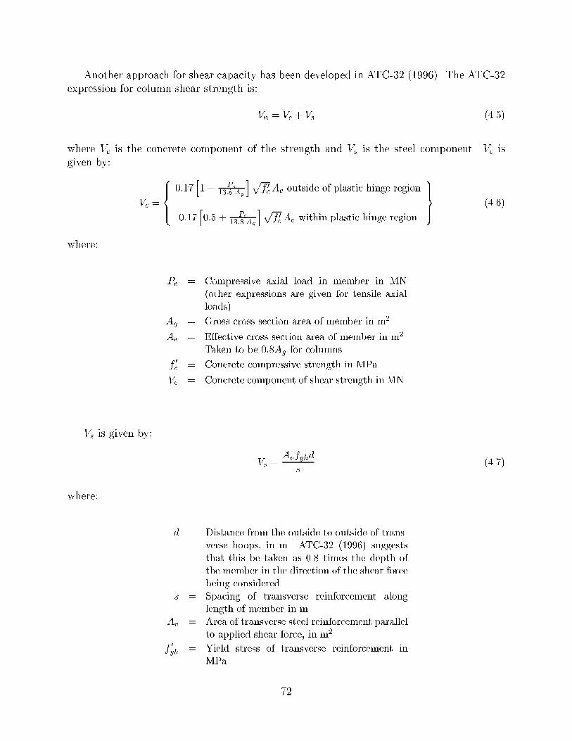
Another approach for shear capacity has been developed in ATC-32 (1996). The ATC-32expression for column shear strength is:

Vn = Vc + Vs (4.5)

where Vc is the concrete component of the strength and Vs is the steel component. Vc isgiven by:

Vc =

8>><>>:

0:17h1 + Pe

13:8 Ag

ipf 0cAe outside of plastic hinge region

0:17h0:5 + Pe

13:8 Ag

ipf 0cAe within plastic hinge region

9>>=>>; (4.6)

where:

Pe = Compressive axial load in member in MN(other expressions are given for tensile axialloads).

Ag = Gross cross section area of member in m2

Ae = E�ective cross section area of member in m2.Taken to be 0:8Ag for columns.

f 0c = Concrete compressive strength in MPa.

Vc = Concrete component of shear strength in MN.

Vs is given by:

Vs =Avfyhd

s(4.7)

where:

d = Distance from the outside to outside of trans-verse hoops, in m. ATC-32 (1996) suggeststhat this be taken as 0.8 times the depth ofthe member in the direction of the shear forcebeing considered.

s = Spacing of transverse reinforcement alonglength of member in m.

Av = Area of transverse steel reinforcement parallelto applied shear force, in m2

f 0yh = Yield stress of transverse reinforcement inMPa.

72

The ATC-32 (1996) shear strength estimates are listed in Table 5.2 in the next chapter.The ATC-32 shear capacity esimates are compared with the values from Table 4.1 accordingto Priestley et al. (1994b) and the shear force demands from earthquake analysis of thebridge. The ATC-32 approach gives brittle shear capacities that are 60-70% of the capacitiesaccording to Priestley et al. (1994b). For the ductile shear strength, the ATC-32 capacityis 70-75% of the Priestley et al. (1994b) capacity for the short columns and about 90%for the tall columns. It has been argued that the conservatism in the ATC-32 approach isappropriate for design. The Priestley et al. (1994b) shear capacity estimates are used in thisstudy because they provide a predictive model without design conservatism.

The exural strength of the columns in the piers is calculated using the exural theory ofreinforced concrete members (Park and Paulay, 1975). The calculations are performed usingthe BIAX analysis program, as described in Section 3.3. The estimates from BIAX comparefavorably with simple estimates of strength based on an equivalent compressive stress blockand elastic-perfectly-plastic steel material. The exural strength of the columns is listed inTable 4.1. The exural deformation capacity is limited by the maximum strain acceptablefor the con�ned concrete and longitudinal reinforcement.

4.3 Nonlinear Static Analysis of Frame 1

The purpose of a nonlinear static analysis (\pushover analysis") of a bridge is to determineamount and distribution of deformation in the components as the lateral displacement in-creases. Events of interest including yielding of components, reaching deformation or straincapacity of components, and brittle failure modes. Of particular interest in the �rst frame ofthe Separation and Overhead bridge is whether the shear capacity of the columns is reachedat longitudinal displacement less than the displacement corresponding to the exural defor-mation capacity of the plastic hinge zones. To examine the question, this section presents apushover analysis of the frame under longitudinal lateral load.

The longitudinal load is applied, as shown in Figure 4.1, in proportion to the tributarymass of each pier. The frame was pushed to a displacement of 450 mm (18 in.) away fromabutment 1. The analysis for longitudinal load towards the abutment would be the same asaway from the abutment for the �rst 254 mm (10 in.) because of the gap between the boxgirder and the backwall (neglecting the lip at the top of the backwall). Beyond that point,the passive pressure of the abutment soil is activated.

The relationship between the longitudinal shear force and top displacement of piers 2and 3 are shown in Figures 4.2 and 4.3, respectively, as determined from the pushoveranalysis. The force-displacement relationship for the entire frame is shown in Figure 4.4.The displacement in the three �gures is in the direction of the frame 1 chord axis so thatthe forces may be compared between �gures. The shear force in Figures 4.2 and 4.3 is inthe longitudinal direction (weak bending direction) for each pier, whereas the force in Figure4.4 is the total force along the frame 1 chord axis. The pushover curves show the typicalreduction of sti�ness due to yielding of the columns in the plastic hinge zones and yieldingof the soil because of displacement of the pile shaft. Selected events in the behavior of the

73

frame are identi�ed in the plots, including yielding of soil springs and yielding of longitudinalsteel.

Also plotted in Figures 4.2 to 4.3 for piers 2 and 3 are the estimates of shear capacity,as discussed in the previous section. Comparing the pushover curve with the shear strengthcurve, it is clear that the shear capacity of the columns will be reached at a displacementsubstantially less than the maximum exural deformation capacity. Pier 2 reaches its shearcapacity at a longitudinal chord displacement of the frame of 135 mm (5.3 in.) and pier 3reaches its shear capacity at a displacement of 170 mm (6.7 in.). The shear capacity for bothcolumns occurs in the brittle/ductile transition zone corresponding to low curvature ductility.Although pier 2 reaches its shear capacity at a longitudinal displacement less than that forpier 3, the two values are fairly close given the uncertainty in the assumptions about materialproperties, particularly the soil properties and ground elevation. This analysis indicates thatpiers 2 and 3 can be expected to fail in shear at a small longitudinal displacement, less than200 mm (7.8 in.), in a brittle/ductile mode with little inelastic exural deformation.

Figure 4.1: Coordinate System for Frame 1

74

0

0.1

0.2

0.3

0.4

0.5

0 50 100 150 200 250 300 350 400 450 500−1000

0

1000

2000

3000

4000

5000

6000

7000

8000

9000

Chord longitudinal displacement (mm)

Loca

l lon

gitu

dina

l she

ar fo

rce

(kN

)

shea

r fo

rce

as a

frac

tion

of p

ier

2 tr

ibut

ary

wei

ght

yield of 1st soil spring, pier 3


yield of 2nd soil spring, pier 3

first steel tension yield

shear failure of pier 2


first steel compression yield

shear capacity

Figure 4.2: Pier 2 Force-Displacement for Longitudinal Static Pushover of Frame 1

75

0

0.1

0.2

0.3

0.4

0.5

0 50 100 150 200 250 300 350 400 450 5000

1000

2000

3000

4000

5000

6000

7000

8000

9000


Loca

l lon

gitu

dina

l she

ar fo

rce

(kN

)

She

ar fo

rce

as a

frac

tion

of p

ier

3 tr

ibut

ary

wei

ght








shear capacity

Figure 4.3: Pier 3 Force-Displacement for Longitudinal Static Pushover of Frame 1

76

0

0.1

0.2

0.3

0.4

0.5

0 50 100 150 200 250 300 350 400 450 5000

2000

4000

6000

8000

10000

12000

14000

16000

18000


Tot

al lo

ngitu

dina

l for

ce (

kN)

Tot

al lo

ngitu

dina

l for

ce a

s a

frac

tion

of fr

ame

wei

ght








Figure 4.4: Frame 1 Force-Displacement for Longitudinal Static Pushover of Frame 1

77

4.4 Superstructure Strength Capacities

Since the superstructure box girder is modeled with linear elastic beam-column elements,the capacity of the box girder must be compared with maximum forces from the earthquakeanalyses. The exural strength of the box girder is evaluated using the equivalent stressblock approach (ACI, 1992; Naaman, 1982).

For example, the weak axis ultimate exural strength of the superstructure in negativebending at pier 2 is estimated as follows, assuming:

fpu = Ultimate stress in prestressing steel, assumedto be 1860 MPa.

fpi = Initial stress in prestressing steel, assumed tobe 75% of fpu, 1400 MPa.

fpei = Initial e�ective stress in prestressing steel, as-sumed to be 85% of fpi or 1190 MPa (to ac-count for losses due to creep, shrinkage, relax-ation, etc.)

= 1190 MPa

Frictional losses are accounted for with the expression (Naaman, 1982):

fpe; pier 2 = fpei e�(� �+K s) (4.8)

where:

� = Coe�cient of angular friction. Assumed to be0.25.

K = Wobble coe�cient, per unit length (m). As-

sumed to be 0.001 radm .

� = Change in angle between force at the anchor-age and the force at pier 2, in radians. Esti-mated to be 0.25 radians.

s = Length of tendon from anchorage point to pier2. Estimated to be 46.6 m.

fpe; pier 2 = E�ective stress in prestressing steel at pier 2.Calculated to be 1060 MPa

78

To calculate the prestress in the tendons under ultimate conditions for an unbondedtendon, ACI (1992) recommends:

fps; pier 2 = fpe; pier 2 + 69 +f 0c

100 �p(in MPa) (4.9)

where:

f 0c = Concrete compressive stress, in MPa. As-sumed to be 34.5 MPa for this strength es-timate.

�p = Prestressing reinforcement ratio,Aps

b dps. Esti-

mated as 1:36� 10�3.

fps; pier 2 = E�ective prestress in tendons at pier 2 underultimate conditions, in MPa. Calculated tobe 1390 MPa.

Aps = Area of prestressing steel, 3:55� 10�2 m2.

b = Width of compression block (so�t width, inthis case), 13.9 m.

dps = Depth from the compression face of the mem-ber to the geometric center of the prestressingsteel at pier 2, 1.88 m.

To estimate the exural strength, the depth of the compression block is determined byiteration until the internal forces are in equilibrium. The results are summarized by:

a = Depth of equivalent compression stress block.Note that compressive strain at the extremecompression �ber is assumed to be 0.003, assuggested by ACI (1992)

= 0:132 m (determined by iteration)

c = Depth from the compression face of the mem-ber to the plastic neutral axis. Taken to bea0:8 , as suggested by ACI (1992).

= 0:166 m

Acc = Approximate area of concrete compressionblock.

= 1:84 m2

79

Three rows of conventional steel reinforcement in the superstructure are considered inthe capacity analysis{#4 bars in the top of the deck slab, #5 bars in the bottom of the deckslab, and #6 bars in the so�t slab. The geometric properties are:

dsteel;bot: = Depth from the compression face of the mem-ber to the geometric center of the bottom bars(25{#6 bars).

= 8:89 � 10�2 m

Asteel;bot: = Area of bottom bar steel.

= 7:13 � 10�3 m2

dsteel;top 1 = Depth from the compression face of the mem-ber to the geometric center of bars in the topof the deck slab (37{#4 bars).

= 2:07 m

Asteel;top 1 = Area of steel in top of deck slab.

= 4:69 � 10�3 m2

dsteel;top 2 = Depth from the compression face of the mem-ber to the geometric center of bars in the bot-tom of the deck slab (50{#5 bars).

= 2:01 m

Asteel;top 2 = Area of steel in bottom of deck slab.

= 9:90 � 10�3 m2

Based on the location of the bars and the location of the plastic neutral axis, the strainand stress in the reinforcement can be estimated:

"steel;bot: = Compression strain in so�t steel.

=(c� dsteel;bot:)

c3:0� 10�3

= 1:39� 10�3

f steel;bot: = Compressive stress in so�t steel.

80

= 279 MPa

"steel;top 1 = Tensile strain in top deck steel.

=(dsteel;top 1 � c)

c3:0� 10�3

= 3:44� 10�2

fsteel;top 1 = Tensile stress in top deck steel.

= 462 MPa

"steel;top 2 = Tensile strain in bottom deck steel.

=(dsteel;top 2 � c)

c3:0� 10�3

= 3:33� 10�2

fsteel;top 2 = Tensile stress in bottom deck steel.

= 462 MPa

The stress in each steel group is calculated based on an elastic-perfectly-plastic modelwith an elastic modulus (Es) of 2:0� 105 MPa and a yield strain ("yield) of 2:31� 10�3.

The estimate of exural strength is then given by summing the moments due to allinternal forces about the compression face, which gives:

Mult = Ultimate exural strength estimate.

= (dsteel;top 1 fsteel;top 1 Asteel;top 1 + dsteel;top 2 fsteel;top 2 Asteel;top 2 + dps fps Aps)

��a

20:85 f 0c Acc + dsteel;bot: fsteel;bot: Asteel;bot:

�= 1:0� 105 kN�m

The exural strength at other locations in the superstructure are summarized in Table 4.2.The shear strength of the box girder is bounded by the limiting values suggested by

Naaman (1982). The total shear strength (Vn) consists of a concrete component and a steelcomponent:

Vn = Vc + Vs

The lower and upper bounds on the concrete component (Vc) of shear strength are given by:

81

Vc =

(0:166

pf 0c Aweb (lower bound)

0:415pf 0c Aweb (upper bound)

)

where:

f 0c = Concrete compressive strength in MPa.

Aweb = E�ective web area of superstructure in m2.

Vc = Concrete component of shear strength in MN.

The steel component of shear strength is given by:

Vs =dp Av fy

s

where:

dp = Depth to prestressing steel from compressionface of member in m.

s = Spacing of transverse reinforcement alonglength of member in m.

Av = Area of transverse steel reinforcement parallelto applied shear force, in m2.

fy = Yield stress of transverse reinforcement inMPa.

Vs = Steel component of shear strength in MN.

As an example of the shear strength calculation, the lower bound on the concrete contri-bution to shear strength at the middle of the �rst span is 2:8 MN based on f 0c = 34:5 MPaand Aweb � 2:83 m2. The steel contribution to shear strength at the same location is 3.3MN based on dp = 1:55 m, s = 0:51 m, Av = 2:38� 10�3 m2, and fy = 462 MPa. The sumof contributions gives the total shear strength of 6.1 MN, or 6100 kN. The bounds on shearstrength of the box girder for the �rst two spans are summarized in Table 4.2.

82

Table4.2:SuperstructureCapacitiesforFrame1

Moment

Shear

Positive

Negative

Positive

Negative

Location

M

+ n

M

� n

V+ n

V� n

kN

�

m

(kip�

in)

kN

�

m

(kip�

in)

kN

(kips)

kN

(kips)

MiddleofFirstSpan

8:2�

104

(7:2�

105)

�

3:9�

104

(�3:5�

105)

6100(1400)to1:0�

104

(2300)

�

6100(�1400)to�

1:0�

104

(�2300)

AtPier2

1:3�

104

(1:2�

105)

�

1:0�

105

(�9:1�

105)

1:1�

104

(2600)to1:6�

104

(3700)

�

1:1�

104

(�2600)to�

1:6�

104

(�3700)

MiddleofSecondSpan

9:2�

104

(8:2�

105)

�

1:8�

104

(�1:6�

105)

7500(1700)to1:3�

104

(2800)

�

7500(�1700)to�

1:3�

104

(�2800)

AtPier3

1:3�

104

(1:2�

105)

�

9:2�

104

(�8:2�

105)

1:1�

104

(2600)to1:6�

104

(3700)

�

1:1�

104

(�2600)to�

1:6�

104

(�3700)

MiddleofThirdSpan

6:4�

104

(5:7�

105)

�

3:4�

104

(�3:0�

105)

6100(1400)to1:0�

104

(2300)

�

6100(�1400)to�

1:0�

104

(�2300)

83

Chapter 5

Earthquake Analysis and Evaluation

of Damage

5.1 Introduction

This chapter presents the earthquake response analysis of the global model of the Separationand Overhead bridge described in Chapter 3. The objective of the analysis is to estimatethe demands on the bridge during the 1994 Northridge earthquake using the six earthquakeground motion records discussed in Section 2.3. The free-�eld ground motion is assumedto be uniform for the supports of the bridge, so spatial variation of the ground motion isnot included. The model includes soil-structure interaction e�ects The role of the verticalground motion component on bridge behavior is examined. Several analyses are repeated toinvestigate the impact of the assumed ground elevation at pier 2.

5.2 Dynamic Analysis

Before commencing with the dynamic analysis, the natural vibration modes of the bridgewere evaluated with the sti�ness under dead load only. For this linearization, the gap ele-ments at the hinges are open, so the global vibration modes represent those of a linearizedmodel with no longitudinal connectivity at the intermediate hinges (similar to a linear \ten-sion" model). Table 5.1 lists the vibration periods and percentage of participating mass inthe three global directions. The lowest vibration mode, with a 2.15 sec period, involves trans-verse vibration of the entire bridge, but with predominant participation of the tall frames.The second mode (1.64 sec period) is the longitudinal vibration of the tall frames. Mode 7with a 0.82 sec period is the longitudinal vibration mode for frame 1. The vertical vibrationmodes have periods of 0.35 sec to 0.45 sec, including modes 14 and 15 in Table 5.1.

The inelastic model of the columns and soil provide hysteretic energy dissipation. Theenergy dissipation in the other components, including radiation damping for the footings, isrepresented as viscous damping using the Rayleigh approach (Clough and Penzien, 1993).Five percent damping is assumed at vibration periods of 2.5 sec and 0.60 sec to represent abroad range of high-participation modes and the softening that takes place as the columns

84

and soil yield. Using standard expressions (Clough and Penzien, 1993), the mass proportionalcoe�cient is � = 0:203 sec�1 and the sti�ness proportional coe�cient is � = 0:00770 sec.With this Rayleigh damping model, the damping coe�cients for the vibration modes arelisted in Table 5.1.

Table 5.1: Summary of Principal Vibration Modes for Global Model

Modal Mass Participation Viscous Dampingas a Fraction of Total Mass percent

Mode No. Period Global X Global Y Global Zsec

1 2.15 0:005 0:316 0:000 4.62 1.64 0:514 0:003 0:000 4.13 1.47 0:000 0:086 0:000 4.04 1.19 0:029 0:004 0:000 4.05 1.03 0:000 0:192 0:000 4.06 0.96 0:016 0:000 0:000 4.17 0.82 0:257 0:000 0:000 4.38 0.81 0:014 0:091 0:000 4.39 0.72 0:000 0:000 0:000 4.510 0.63 0:004 0:000 0:008 4.911 0.56 0:000 0:000 0:000 5.212 0.56 0:003 0:000 0:000 5.213 0.53 0:005 0:051 0:000 5.414 0.45 0:002 0:000 0:018 6.115 0.40 0:002 0:000 0:046 6.7

Sum - 0:851 0:743 0:072

The dynamic analysis uses the implicit Newmark integration scheme with the event-to-event state determination strategy in DRAIN-3DX. To reduce the number of events andhence computation time, the force overshoot factors for event determination are not greaterthan 1% of the yield force for the nonlinear elements, and less than 0.1% for many of theelements. Based on a trade-o� between accuracy and amount of computation, an integrationtime step of 0.01 sec was used for all dynamic analyses. The accuracy of the solution wasmonitored by the unbalanced forces and error in energy terms.

The model has approximately 750 degrees-of-freedom. The computation time for 2000time steps is approximately 30-45 minutes (depending on the ground motion) on a DigitalAlphaStation 500 workstation computer.

5.3 Evaluation of Earthquake Response

5.3.1 Shear Force Demands

The maximum shear forces in the nine piers are listed in Table 5.2 for each of the six groundmotion records. The shear forces are the maximum value, over the response history, in thelocal longitudinal and transverse direction, for each pier. The maximum shear force can becompared with the estimates of shear strength, as discussed in Section 4.2. When comparingthe column shear demands with capacities, it should be emphasized that the columns hada small amount of transverse reinforcement with #5 hoops at 300 mm (12 in.) and cross-

85

bars. The bridge satis�ed the pre-1971 design speci�cation, but the coluumns clearly haveinadequate shear capacity according to capacity-design principles.

Considering the estimates of column shear strength using the Priestley et al. (1994b)theory, the longitudinal shear force demand in pier 2 exceeds the brittle capacity for the Syl-mar, Jensen, Newhall, and Hutchings, ICN ground motion records. All the records producelongitudinal shear forces greater than the ductile shear capacity. The longitudinal shear forcedemand in pier 3 does not exceed the brittle capacity for any record, although the Sylmarand Hutchings, ICN simulated records reach 90% of the brittle capacity; the longitudinalshear force in pier 3 exceeds the ductile capacity for all the ground motion records, with theexception of the lower-amplitude Arleta record. The transverse shear forces in piers 2 and 3are greater than the ductile shear capacity for most records, but less than the brittle shearcapacity.

The second frame of the bridge is supported by piers 4 and 5, for which the maximumlongitudinal shear forces for all records are less than the ductile shear capacity of the piers.Several of the records produce transverse shear forces greater than the ductile shear capacityof piers 4 or 5, but less than the brittle capacity. For piers 6 to 9 the maximum shear forcesfrom the demand analysis are less than the ductile shear capacity of the piers. At the otherend of the bridge, pier 10 is relatively short and the longitudinal shear force exceeds theductile capacity for the Sylmar and Hutchings, ICN records.

Examining the pier response in more detail, Figures 5.1 to 5.6 show the shear force de-mand history in piers 2, 3, and 4 for the six ground motion records, each including thevertical ground motion component. The computed transverse, longitudinal, and resultantshear forces for the pier are plotted as a function of time. The longitudinal response domi-nates the shear force demand for these three piers. Also plotted on the shear force history�gures for piers 2 and 3 are the shear capacity estimates from Priestley et al. (1994b). Thetransition from brittle to ductile shear capacity is based on the curvature ductility of thecolumns as obtained from the demand analysis.

When interpreting the shear demands and capacity estimates it must be recognized thatthere are many assumptions in the demand and capacity models and the selection of earth-quake ground motion representative of the site. Nevertheless, the shear force histories provideinsight into the behavior of the bridge in the 1994 Northridge earthquake. Considering thecomputed response to the Symlar record in Figure 5.1, the �rst large shear excursion forpiers 2 and 3 reaches the theoretical shear capacity between the brittle and ductile zones asthe bridge displaces longitudinally away from abutment 1. The second large response pulseexceeds the ductile shear capacity by nearly a factor of two as the bridge moves longitudi-nally towards abutment 1. The shear force demand in pier 4 is less than the ductile shearcapacity for that pier. The shear response computed for the Newhall and Jenson records inFigures 5.2 and 5.3, respectively, is similar to the behavior noted for the Sylmar record. Thelow amplitude of the Arleta record gives shear demands less than the ductile capacity for thepiers, as shown in Figure 5.4. The computed shear demands for the two simulated recordsin Figures 5.5 and 5.6 give more cycles of peak response than the recorded ground motions.According to the analysis for these ground motions, piers 2 and 3 have shear force demandsgreater than the degraded shear capacity after several cycles in the case of the Hutchings,ICN simulated record. For the Horton simulated record, both piers and 2 and 3 just reach

86

the shear capacity after several cycles.Another view of the computed column shear demands is shown in Figures 5.7 to 5.24, in

which the shear force locus for each pier is plotted as longitudinal shear force against trans-verse shear force. The loci plots also show the brittle and ductile envelopes of shear capacity,which are elliptical in shape based on the longitudinal and transverse shear capacities usingPriestley et al. (1994b). Considering the computed response to the Sylmar record in Figure5.7, the demands in piers 2 and 3 pierce the ductile shear capacity envelope, primarily inthe longitudinal direction, whereas the pier 4 shear demand only touches the ductile shearcapacity envelope. In Figures 5.8 and 5.9 the shear demand locus just touches the ductilecapacity envelope for piers 5 and 10; piers 6 to 9 have adequate shear capacity accordingto the analysis. The computed responses for the Newhall and Jensen records, Figures 5.10to 5.15, are similar to that for Sylmar. It is interesting to note the predominant transverseresponse for the tall piers 5 to 7 in Figure 5.14. The Arleta record produces relatively smallshear demands, as shown in Figures 5.16 to 5.18.

The computed shear response for the Hutchings, ICN simulated record is plotted inFigures 5.19 to 5.21. The response follows the general trends observed for the recordedground motion records, but the shear force loci have more bi-directional response and agreater number of peak excursions. The shear force response to the Horton simulated record,Figures 5.22 to 5.24, does not have as many excursions beyond the ductile capacity as theHutchings, ICN simulated record. The response for the short piers near the ends of thebridge is predominantly longitudinal and the response of the tall piers in the middle of thebridge is predominantly transverse.

87

Table5.2:MaximumColumnShearForceDemandsandCapacityEstimate

Pier2

Pier3

Pier4

Pier5

Pier6

Pier7

Pier8

Pier9

Pier10

Record

kN

kN

kN

kN

kN

kN

kN

kN

kN

Arleta

WithVerticalMotion

Longitudinal

-4710

-2900

-1320

1260

997

582

981

831

1890

Transverse

3530

4280

3440

3150

1680

1220

1230

856

-1920

WithoutVertical

Motion

Longitudinal

-4670

-2860

-1280

1120

985

583

991

841

1880

Transverse

3570

4270

3380

3170

1650

1210

1220

910

-1920

Sylmar

WithVerticalMotion

Longitudinal

-10100

-7260

-3500

-3170

-2600

-1370

-2720

-2320

-4380

Transverse

5060

5760

4570

-3500

2700

1920

-2630

-1520

-3680

WithoutVertical

Motion

Longitudinal

-9950

-7170

-3450

-3150

-2630

-1390

-2740

-2380

-4320

Transverse

4920

5790

4590

-3500

2720

1920

-2610

-1550

-3790

Jensen

WithVerticalMotion

Longitudinal

-8220

-6450

-2960

2830

2140

1170

1990

1740

3460

Transverse

4510

-5990

-3870

-6330

-3440

2200

2630

1940

4430

WithoutVertical

Motion

Longitudinal

-8370

-6200

-2830

2660

2060

1100

2013

1770

3330

Transverse

4560

-6150

-3890

-6350

3380

-2170

2640

1930

4400

Horton,Pier3

WithVerticalMotion

Longitudinal

-7240

4870

-2290

-1960

1930

1130

2230

1970

3720

Transverse

5350

-6620

-4540

-5960

3390

2330

2530

-1540

-3910

WithoutVertical

Motion

Longitudinal

-7310

4870

2230

-2010

1970

1160

2220

1970

3730

Transverse

5590

6670

-4540

-6050

3400

2340

2500

-1520

-3880

Newhall

WithVerticalMotion

Longitudinal

-9050

-6730

3260

-2950

-2220

1270

-2350

1980

-3680

Transverse

4730

4750

5140

-5300

-2230

-1810

2000

-1440

3020

WithoutVertical

Motion

Longitudinal

-9110

-6690

-3180

-2850

-2130

1190

2170

1880

-3590

Transverse

5210

-5200

5350

-5380

2230

-1760

1970

-1360

2760

Hutchings,

ICN

WithVerticalMotion

Longitudinal

9590

7580

3520

3530

2970

1660

2850

2650

4460

Transverse

-6240

8970

6700

4430

3150

2050

2330

2080

-3750

WithoutVertical

Motion

Longitudinal

9560

7410

3330

3330

2800

1510

2800

2580

-4290

Transverse

6190

8930

6600

-4800

2940

1900

2190

2100

3700

Capacity,

(Priestley

etal.,1994b)

Brittle

Longitudinal

8170

8100

7400

7360

6840

7270

7320

7400

7670

Transverse

9360

9260

8350

8300

7270

7330

7370

7450

8740

Ductile

Longitudinal

4400

4330

3630

3590

3550

3680

3720

3810

3890

Transverse

5590

5490

4580

4530

3980

3740

3780

3860

4970

Capacity,

(ATC-32,

1996)

Brittle

Longitudinal

4850

4840

4660

4660

4670

4930

4780

4910

4860

Transverse

5250

5240

5060

5060

4880

4960

4810

4930

5260

Ductile

Longitudinal

3210

3200

3020

3020

3240

3370

3220

3340

3220

Transverse

3610

3600

3420

3520

3450

3390

3250

3370

3620

88

−1

−0.5

0

0.5

1x 10

4 Pier 2S

hear

For

ce (

kN)

CapacityVector Sum

Longitudinal Transverse

−1

−0.5

0

0.5

1x 10

4 Pier 3

She

ar F

orce

(kN

)

CapacityVector Sum

LongitudinalTransverse

0 2 4 6 8 10 12 14 16 18 20−1

−0.5

0

0.5

1x 10

4 Pier 4

Time (sec)

She

ar F

orce

(kN

)

Vector Sum


Figure 5.1: Column Shear Force Demand vs. Capacity, Sylmar Ground Motion

89

−1

−0.5

0

0.5

1x 10

4 Pier 2S

hear

For

ce (

kN)

CapacityVector Sum


−1

−0.5

0

0.5

1x 10

4 Pier 3

She

ar F

orce

(kN

)

CapacityVector Sum


0 2 4 6 8 10 12 14 16 18 20−1

−0.5

0

0.5

1x 10

4 Pier 4

Time (sec)

She

ar F

orce

(kN

)

Vector Sum


Figure 5.2: Column Shear Force Demand vs. Capacity, Newhall Ground Motion

90

−1

−0.5

0

0.5

1x 10

4 Pier 2S

hear

For

ce (

kN)

CapacityVector Sum


−1

−0.5

0

0.5

1x 10

4 Pier 3

She

ar F

orce

(kN

)

CapacityVector Sum


0 2 4 6 8 10 12 14 16 18 20−1

−0.5

0

0.5

1x 10

4 Pier 4

Time (sec)

She

ar F

orce

(kN

)

Vector Sum


Figure 5.3: Column Shear Force Demand vs. Capacity, Jensen Ground Motion

91

−1

−0.5

0

0.5

1x 10

4 Pier 2S

hear

For

ce (

kN) Capacity Vector Sum


−1

−0.5

0

0.5

1x 10

4 Pier 3

She

ar F

orce

(kN

) CapacityVector Sum


0 2 4 6 8 10 12 14 16 18 20−1

−0.5

0

0.5

1x 10

4 Pier 4

Time (sec)

She

ar F

orce

(kN

)

Vector Sum


Figure 5.4: Column Shear Force Demand vs. Capacity, Arleta Ground Motion

92

−1

−0.5

0

0.5

1x 10

4 Pier 2S

hear

For

ce (

kN) Capacity

Vector Sum


−1

−0.5

0

0.5

1x 10

4 Pier 3

She

ar F

orce

(kN

) Capacity

Vector Sum


0 2 4 6 8 10 12 14 16 18 20−1

−0.5

0

0.5

1x 10

4 Pier 4

Time (sec)

She

ar F

orce

(kN

)

Vector Sum


Figure 5.5: Column Shear Force Demand vs. Capacity, Hutchings et al. (1996) ICN Simu-lated Ground Motion

93

−1

−0.5

0

0.5

1x 10

4 Pier 2S

hear

For

ce (

kN) Capacity

Vector Sum

Longitudinal

Transverse

−1

−0.5

0

0.5

1x 10

4 Pier 3

She

ar F

orce

(kN

) CapacityVector Sum


0 2 4 6 8 10 12 14 16 18 20−1

−0.5

0

0.5

1x 10

4 Pier 4

Time (sec)

She

ar F

orce

(kN

)

Vector Sum

Longitudinal

Transverse

Figure 5.6: Column Shear Force Demand vs. Capacity, Horton et al. (1995) Pier 3 SimulatedGround Motion

94

−1

−0.5

0

0.5

1x 10

4 Pier 2

Tra

nsve

rse

She

ar (

kN) Brittle Capacity

Ductile Capacity

−1

−0.5

0

0.5

1x 10

4 Pier 3

Tra

nsve

rse

She

ar (

kN)

Brittle Capacity

Ductile Capacity

−2.5 −2 −1.5 −1 −0.5 0 0.5 1 1.5 2 2.5

x 104

−1

−0.5

0

0.5

1x 10

4 Pier 4

Longitudinal Shear (kN)

Tra

nsve

rse

She

ar (

kN)

Brittle Capacity

Ductile Capacity

Figure 5.7: Column Shear Force (Piers 2 to 4), Longitudinal vs. Transverse, Sylmar GroundMotion

−1

−0.5

0

0.5

1x 10

4 Pier 5

Tra

nsve

rse

She

ar (


Ductile Capacity

−1

−0.5

0

0.5

1x 10

4 Pier 6

Tra

nsve

rse

She

ar (


Ductile Capacity

−2.5 −2 −1.5 −1 −0.5 0 0.5 1 1.5 2 2.5

x 104

−1

−0.5

0

0.5

1x 10

4 Pier 7


Tra

nsve

rse

She

ar (


Ductile Capacity


95

−1

−0.5

0

0.5

1x 10

4 Pier 8

Tra

nsve

rse

She

ar (


Ductile Capacity

−1

−0.5

0

0.5

1x 10

4 Pier 9

Tra

nsve

rse

She

ar (


Ductile Capacity

−2.5 −2 −1.5 −1 −0.5 0 0.5 1 1.5 2 2.5

x 104

−1

−0.5

0

0.5

1x 10

4 Pier 10


Tra

nsve

rse

She

ar (


Ductile Capacity


−1

−0.5

0

0.5

1x 10

4 Pier 2

Tra

nsve

rse

She

ar (


Ductile Capacity

−1

−0.5

0

0.5

1x 10

4 Pier 3

Tra

nsve

rse

She

ar (


Ductile Capacity

−2.5 −2 −1.5 −1 −0.5 0 0.5 1 1.5 2 2.5

x 104

−1

−0.5

0

0.5

1x 10

4 Pier 4


Tra

nsve

rse

She

ar (

kN)

Brittle Capacity

Ductile Capacity

Figure 5.10: Column Shear Force (Piers 2 to 4), Longitudinal vs. Transverse, NewhallGround Motion

96

−1

−0.5

0

0.5

1x 10

4 Pier 5

Tra

nsve

rse

She

ar (


Ductile Capacity

−1

−0.5

0

0.5

1x 10

4 Pier 6

Tra

nsve

rse

She

ar (


Ductile Capacity

−2.5 −2 −1.5 −1 −0.5 0 0.5 1 1.5 2 2.5

x 104

−1

−0.5

0

0.5

1x 10

4 Pier 7


Tra

nsve

rse

She

ar (


Ductile Capacity


−1

−0.5

0

0.5

1x 10

4 Pier 8

Tra

nsve

rse

She

ar (


Ductile Capacity

−1

−0.5

0

0.5

1x 10

4 Pier 9

Tra

nsve

rse

She

ar (


Ductile Capacity

−2.5 −2 −1.5 −1 −0.5 0 0.5 1 1.5 2 2.5

x 104

−1

−0.5

0

0.5

1x 10

4 Pier 10


Tra

nsve

rse

She

ar (


Ductile Capacity


97

−1

−0.5

0

0.5

1x 10

4 Pier 2

Tra

nsve

rse

She

ar (


Ductile Capacity

−1

−0.5

0

0.5

1x 10

4 Pier 3

Tra

nsve

rse

She

ar (


Ductile Capacity

−2.5 −2 −1.5 −1 −0.5 0 0.5 1 1.5 2 2.5

x 104

−1

−0.5

0

0.5

1x 10

4 Pier 4


Tra

nsve

rse

She

ar (


Ductile Capacity

Figure 5.13: Column Shear Force (Piers 2 to 4), Longitudinal vs. Transverse, Jensen GroundMotion

−1

−0.5

0

0.5

1x 10

4 Pier 5

Tra

nsve

rse

She

ar (


Ductile Capacity

−1

−0.5

0

0.5

1x 10

4 Pier 6

Tra

nsve

rse

She

ar (


Ductile Capacity

−2.5 −2 −1.5 −1 −0.5 0 0.5 1 1.5 2 2.5

x 104

−1

−0.5

0

0.5

1x 10

4 Pier 7


Tra

nsve

rse

She

ar (


Ductile Capacity

Figure 5.14: Column Shear Force (Piers 5 to 7), Longitudinal vs. Transverse, Jensen GroundMotion

98

−1

−0.5

0

0.5

1x 10

4 Pier 8

Tra

nsve

rse

She

ar (


Ductile Capacity

−1

−0.5

0

0.5

1x 10

4 Pier 9

Tra

nsve

rse

She

ar (


Ductile Capacity

−2.5 −2 −1.5 −1 −0.5 0 0.5 1 1.5 2 2.5

x 104

−1

−0.5

0

0.5

1x 10

4 Pier 10


Tra

nsve

rse

She

ar (


Ductile Capacity

Figure 5.15: Column Shear Force (Piers 8 to 10), Longitudinal vs. Transverse, JensenGround Motion

−1

−0.5

0

0.5

1x 10

4 Pier 2

Tra

nsve

rse

She

ar (


Ductile Capacity

−1

−0.5

0

0.5

1x 10

4 Pier 3

Tra

nsve

rse

She

ar (


Ductile Capacity

−2.5 −2 −1.5 −1 −0.5 0 0.5 1 1.5 2 2.5

x 104

−1

−0.5

0

0.5

1x 10

4 Pier 4


Tra

nsve

rse

She

ar (


Ductile Capacity

Figure 5.16: Column Shear Force (Piers 2 to 4), Longitudinal vs. Transverse, Arleta GroundMotion

99

−1

−0.5

0

0.5

1x 10

4 Pier 5

Tra

nsve

rse

She

ar (


Ductile Capacity

−1

−0.5

0

0.5

1x 10

4 Pier 6

Tra

nsve

rse

She

ar (


Ductile Capacity

−2.5 −2 −1.5 −1 −0.5 0 0.5 1 1.5 2 2.5

x 104

−1

−0.5

0

0.5

1x 10

4 Pier 7


Tra

nsve

rse

She

ar (


Ductile Capacity


−1

−0.5

0

0.5

1x 10

4 Pier 8

Tra

nsve

rse

She

ar (


Ductile Capacity

−1

−0.5

0

0.5

1x 10

4 Pier 9

Tra

nsve

rse

She

ar (


Ductile Capacity

−2.5 −2 −1.5 −1 −0.5 0 0.5 1 1.5 2 2.5

x 104

−1

−0.5

0

0.5

1x 10

4 Pier 10


Tra

nsve

rse

She

ar (


Ductile Capacity


100

−1

−0.5

0

0.5

1x 10

4 Pier 2

Tra

nsve

rse

She

ar (


Ductile Capacity

−1

−0.5

0

0.5

1x 10

4 Pier 3

Tra

nsve

rse

She

ar (


Ductile Capacity

−2.5 −2 −1.5 −1 −0.5 0 0.5 1 1.5 2 2.5

x 104

−1

−0.5

0

0.5

1x 10

4 Pier 4


Tra

nsve

rse

She

ar (


Ductile Capacity

Figure 5.19: Column Shear Force (Piers 2 to 4), Longitudinal vs. Transverse, Hutchings etal. (1996) ICN Simulated Ground Motion

−1

−0.5

0

0.5

1x 10

4 Pier 5

Tra

nsve

rse

She

ar (

kN)

Brittle Capacity

Ductile Capacity

−1

−0.5

0

0.5

1x 10

4 Pier 6

Tra

nsve

rse

She

ar (


Ductile Capacity

−2.5 −2 −1.5 −1 −0.5 0 0.5 1 1.5 2 2.5

x 104

−1

−0.5

0

0.5

1x 10

4 Pier 7


Tra

nsve

rse

She

ar (


Ductile Capacity


101

−1

−0.5

0

0.5

1x 10

4 Pier 8

Tra

nsve

rse

She

ar (


Ductile Capacity

−1

−0.5

0

0.5

1x 10

4 Pier 9

Tra

nsve

rse

She

ar (


Ductile Capacity

−2.5 −2 −1.5 −1 −0.5 0 0.5 1 1.5 2 2.5

x 104

−1

−0.5

0

0.5

1x 10

4 Pier 10


Tra

nsve

rse

She

ar (


Ductile Capacity


−1

−0.5

0

0.5

1x 10

4 Pier 2

Tra

nsve

rse

She

ar (


Ductile Capacity

−1

−0.5

0

0.5

1x 10

4 Pier 3

Tra

nsve

rse

She

ar (


Ductile Capacity

−2.5 −2 −1.5 −1 −0.5 0 0.5 1 1.5 2 2.5

x 104

−1

−0.5

0

0.5

1x 10

4 Pier 4


Tra

nsve

rse

She

ar (


Ductile Capacity

Figure 5.22: Column Shear Force (Piers 2 to 4), Longitudinal vs. Transverse, Horton et al.(1995) Pier 3 Simulated Ground Motion

102

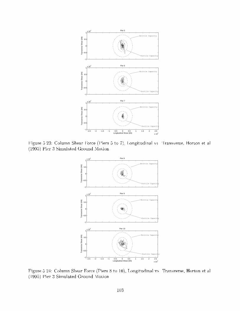
−1

−0.5

0

0.5

1x 10

4 Pier 5

Tra

nsve

rse

She

ar (


Ductile Capacity

−1

−0.5

0

0.5

1x 10

4 Pier 6

Tra

nsve

rse

She

ar (


Ductile Capacity

−2.5 −2 −1.5 −1 −0.5 0 0.5 1 1.5 2 2.5

x 104

−1

−0.5

0

0.5

1x 10

4 Pier 7


Tra

nsve

rse

She

ar (


Ductile Capacity


−1

−0.5

0

0.5

1x 10

4 Pier 8

Tra

nsve

rse

She

ar (


Ductile Capacity

−1

−0.5

0

0.5

1x 10

4 Pier 9

Tra

nsve

rse

She

ar (


Ductile Capacity

−2.5 −2 −1.5 −1 −0.5 0 0.5 1 1.5 2 2.5

x 104

−1

−0.5

0

0.5

1x 10

4 Pier 10


Tra

nsve

rse

She

ar (


Ductile Capacity


103

5.3.2 Examination of Other Structural Demands

The analyses presented in the previous section show that piers 2 and 3 had de�cient shearcapacity for the estimated demands in the 1994 Northridge earthquake. The other piers inthe bridge, with the exception of pier 10, had adequate shear capacity for the Northridgeearthquake ground motions. (The columns are shear-critical and would be expected to failin larger ground motions.) The computed history of shear force demands in piers 2 and3 show that the capacity is reached early in the earthquake during the �rst large cycle oflongitudinal displacement of the bridge.

To examine whether inadequate shear capacity of piers 2 and 3 initiated the collapse ofthe �rst frame, other demands in the bridge at the time that the column shear capacityis reached must be compared with the corresponding capacity estimates. The followingcomputed response quantities are examined: shear force and bending moment of the boxgirder superstructure; the bending moment in the pier shafts at the longitudinal bar cuto�points; and opening displacement of the intermediate hinges. Table 5.3 lists for each quantitythe maximum ratio of demand to capacity, where the capacity is given in Chapter 4 and thedemand is the maximum response to the time the shear capacity in pier 2 is exhausted. Thedemand-capacity comparison is for the largest ground motion records, Sylmar, Newhall, andtbe Hutchings, ICN simulated record.

The �rst section of Table 5.3 gives the demand-capacity ratio for bending moment in thesuperstructure for the �rst three spans. For the Sylmar record and Hutchings, ICN simulatedrecord the maximum ratio is 0.74 and 0.85, respectively, for negative bending at the middlethe span between piers 2 and 3. Otherwise the bending moment demand-capacity ratio doesnot exceed 0.60.

The computed response for the Newhall record to the time at which pier 2 reaches thetheoretical shear capacity shows an important e�ect of the vertical ground motion on boxgirder forces. These e�ects do not occur for the other ground motion records. The maximumbending moment in the box girder for Newhall without the vertical ground motion (onlyincluding longitudinal and transverse ground motion components) is limited to 0.63 of thecapacity for negative bending of span 2 at pier 3. When all three ground components ofthe Newhall record are included in the earthquake analysis, the demand-capacity ratio forthe box girder bending moment is 2.62 and 1.92 for positive bending at piers 2 and 3. Asdiscussed in conjunction with Figure 2.21 in Section 2.3.3, the vertical component of theNewhall record has signi�cant energy in the period range of the vertical vibration modesof the superstructure which leads to the reversal of bending moments over piers 2 and 3.Although the box girder has some exural ductility, the response analysis indicates thatthe positive moment reinforcement could have yielded very early in the earthquake responsebefore piers 2 and 3 reached their shear capacity. It should be noted that current bridgedesign practice is to avoid inelastic deformation in the superstructure.

As discussed in Section 1.3, one postulated cause for the failure of frame 1 was a punchingshear failure of the box girder at pier 3. The second section of Table 5.3 gives the demand/capacity ratio for shear force in the box girder to the time piers 2 and 3 reach their shearcapacity. The largest demand-capacity ratio is 0.74 for the Newhall record including thevertical ground motion component. The largest ratio for the other records is 0.61. The

104

response analyses indicate that the box girder had su�cient shear capacity for the postulatedground motions.

The reduced capacity in the shaft below cuto� of the longitudinal reinforcement was notincluded in the model, as discussed in Section 3.3.3. To examine this issue, the third section ofTable 5.3 gives the ratio of maximum bending moment in the shafts below the cuto� relativeto the exural capacity below the cuto�. The exural demand on the piers 2 and 3 shafts donot exceed the exural capacity. The demand-capacity ratio exceeds unity primarily for piers6 and 8 to 10. The largest ratio is 1.4, indicating that a small amount of exural yieldingmay have occurred in the pier shafts below the longitudinal bar cuto�. The demand ratiois small enough that the actual strength of the shaft may have accommodated the demandwith minor yielding, recognizing that the surrounding soil provides some con�nement.

The last section of Table 5.3 gives the maximum opening displacements at the fourintermediate hinges in the bridge. The opening displacement at hinge 4 is less than the20% of the hinge seat width for all of the ground motion records. With the small hingedisplacements predicted from the model and postulated ground motion, it is unlikely thatthe failure of frame 1 initiated with unseating at hinge 4. The largest demand-capacityratio for the other hinges is 0.43 for hinge 5. The post-earthquake inspection of the bridgerevealed local damage at hinge 5 caused by impact of the box girders. Hinges that undergolarge opening displacements may experience pounding when they close.

5.4 E�ect of Pier 2 Ground Elevation

As observed by Priestley et al. (1994a) the ground elevation at pier 2 may have been approx-imately 1.5 m (5 ft) higher than the design drawings indicate. To investigate the e�ect ofthe ground elevation of pier 2, an alternate model is considered in which the pier 2 groundlevel is 1.5 m (5 ft) higher than the original model. The e�ective overburden elevation forthe purpose of estimating the properties of the p-y soil springs remains unchanged. Thealternate model is compared with the original model for the three largest ground motions(Newhall, Sylmar, and Hutchings, ICN), including the vertical components. The summaryresults are given for the entire response history, not just to the time of shear failure of piers2 and 3.

The trends in column shear demand relative to capacity observed in Section 5.3.1 for theoriginal model are evident in the model with a higher pier 2 ground elevation. Table 5.4summarizes the maximum shear force demand for the two models. The longitudinal shearforce in pier 2 increases between 13-16% for the shorter pier 2 compared with the originalmodel. Shortening pier 2 decreases the maximum longitudinal shear force on pier 3 by 1-3onthe shear forces in the other piers.

The histories of shear force demands for the alternate model with higher ground elevationof pier 2 are shown in Figures 5.25 to 5.27. The computed responses for the Newhall recordand Hutchings, ICN simulated record clearly that pier 2 reaches its shear capacity in thebrittle-ductile transition zone prior to pier 3 reaching its capacity. As with the referencemodel, the response analysis for the Sylmar record shows that piers 2 and 3 reach theirrespective capacities at approximately the same time. However, the demand-to-capacityratio is larger for pier 2 than pier 3 at the time the capacity is reached.

105

Table5.3:DemandsandCapacitiesatTimeofShearFailureofPier2

SuperstructureMoments

NewhallwithVertical

NewhallwithoutVertical

Sylmar

Hutchings,ICN

Location

Capacity

NetDemand

Demand/Capacity

NetDemand

Demand/Capacity

NetDemand

Demand/Capacity

NetDemand

Demand/Capacity

kN�

m

kN�

m

kN�

m

kN�

m

kN�

m

Span1

Mid-span

Max

8:2�

104

2:4�

104

0:30

7:0�

103

0:09

2:1�

104

0:25

2:5�

104

0:31

Min

�

3:9�

104

�

3:4�

104

0:87

�

2:6�

104

0:67

�

2:5�

104

0:63

�

2:2�

104

0:57

Right

Max

1:3�

104

8:8�

103

0:67

�

1:0�

104

0:10

�

7:4�

103

0:07

3:2�

103

0:25

Min

�

1:0�

105

�

6:9�

104

0:67

�

4:7�

104

0:46

�

5:3�

104

0:52

�

4:5�

104

0:44

Span2

Left

Max

1:3�

104

3:4�

104

2:62

3:6�

103

0:27

5:9�

103

0:45

�

5:9�

103

0:06

Min

�

1:0�

104

�

4:9�

104

0:48

3:2�

104

0:31

�

4:7�

104

0:46

�

5:8�

104

0:57

Mid-span

Max

9:2�

104

1:7�

104

0:18

4:7�

103

0:05

1:1�

104

0:12

3:4�

103

0:04

Min

�

1:8�

104

�

2:6�

104

1:41

�

1:2�

104

0:63

�

1:4�

104

0:74

�

1:6�

104

0:85

Right

Max

1:3�

104

0

0

�

2:0�

104

0:22

�

1:5�

104

0:16

0

0

Min

�

9:2�

104

�

8:1�

104

0:88

�

5:8�

104

0:63

�

6:6�

104

0:72

�

5:6�

104

0:60

Span3

Left

Max

1:3�

104

2:5�

104

1:92

�

1:1�

104

0:12

�

8:0�

103

0:09

�

2:0�

104

0:22

Min

�

9:2�

104

�

4:6�

104

0:50

�

3:3�

104

0:36

�

4:3�

104

0:47

�

4:6�

104

0:50

Mid-span

Max

6:4�

104

4:6�

104

0:72

1:4�

104

0:21

1:8�

104

0:28

1:9�

104

0:30

Min

�

3:4�

104

�

1:8�

104

0:54

4:1�

103

0:06

�

6:8�

103

0:20

�

9:6�

103

0:29

SuperstructureShearForces

NewhallwithVertical


Sylmar

Hutchings,ICN

Location

Capacity

NetDemand

Demand/Capacity

NetDemand

Demand/Capacity

NetDemand

Demand/Capacity

NetDemand

Demand/Capacity

kN

kN

kN

kN

kN

Span1

Mid-span

6:1�

103

2:6�

103

0:42

1:8�

103

0:30

2:0�

103

0:32

1:8�

103

0:29

Right

1:1�

104

8:1�

103

0:73

5:7�

103

0:52

6:6�

103

0:60

6:3�

103

0:58

Span2

Left

1:1�

104

6:6�

103

0:60

5:3�

103

0:48

6:5�

103

0:59

6:2�

103

0:56

Mid-span

7:5�

103

1:2�

103

0:15

9:5�

102

0:13

1:3�

103

0:18

1:2�

103

0:16

Right

1:1�

104

7:4�

103

0:67

6:2�

103

0:56

6:7�

103

0:61

6:2�

103

0:56

Span3

Left

1:1�

104

8:2�

103

0:74

5:1�

103

0:47

6:4�

103

0:58

6:1�

103

0:55

Mid-span

6:1�

103

9:1�

102

0:15

2:8�

102

0:05

6:1�

102

0:10

6:9�

102

0:11

SubgradePierMomentsatBarCut{o�Location(WeakAxisOnly)

NewhallwithVertical


Sylmar

Hutchings,ICN

Location

Capacity

NetDemand

Demand/Capacity

NetDemand

Demand/Capacity

NetDemand

Demand/Capacity

NetDemand

Demand/Capacity

kN�

m

kN�

m

kN�

m

kN�

m

kN�

m

Pier2

1:2�

104

3:7�

103

0:31

3:8�

103

0:31

5:0�

103

0:42

3:9�

103

0:32

Pier3

1:2�

104

7:6�

103

0:63

8:0�

103

0:66

4:9�

103

0:40

6:5�

103

0:54

Pier4

1:2�

104

1:4�

104

1:17

1:3�

104

1:11

1:7�

104

0:39

1:1�

104

0:89

Pier5

1:2�

104

8:5�

103

0:70

7:9�

103

0:66

1:0�

104

0:83

5:3�

103

0:44

Pier6

1:6�

104

1:9�

104

1:20

1:8�

104

1:16

1:7�

104

1:09

9:6�

103

0:61

Pier7

1:9�

104

1:9�

104

0:96

1:7�

104

0:86

1:8�

104

0:91

9:5�

103

0:49

Pier8

1:9�

104

2:5�

104

1:31

2:5�

104

1:31

2:5�

104

1:30

1:5�

104

0:79

Pier9

1:9�

104

2:5�

104

1:27

2:3�

104

1:22

2:4�

104

1:26

1:5�

104

0:80

Pier10

1:2�

104

1:5�

104

1:28

1:6�

104

1:29

1:7�

104

1:39

8:5�

103

0:70

HingeDisplacement

NewhallwithVertical


Sylmar

Hutchings,ICN

Location

Capacity

NetDemand

Demand/Capacity

NetDemand

Demand/Capacity

NetDemand

Demand/Capacity

NetDemand

Demand/Capacity

mm

mm

mm

mm

mm

Hinge4

330

55

0:17

56

0:17

43

0:13

28

0:08

Hinge5

330

140

0:42

140

0:43

140

0:43

38

0:11

Hinge7

330

37

0:11

37

0:11

18

0:05

29

0:09

Hinge9

330

16

0:05

15

0:05

9

0:03

26

0:08

106

The e�ect of the pier 2 ground elevation on the displacements of the bridge is summarizedin Tables 5.5 to 5.7. The shorter pier 2 reduces the displacement at the top of the piers forframe 1 6-10% because of the increased sti�ness of the pier. However, the larger forces in theframe 1 piers produce larger displacement of the piers at the ground surface because of theof the increased forces on the soil. In Table 5.6, the shorter pier 2 increases the displacementat the ground surface for pier 2 from 38-56 mm (1.5-2.2 in.) to 66-81 mm (2.6-3.2 in.). Thee�ect of the pier 2 ground elevation is further con�rmed in Table 5.7, which shows that themaximum curvature in pier 2 increases by 10-30% with the increased ground elevation. Themaximum curvature for the other piers generally decreases with the increase in the assumedpier 2 ground elevation. Table 5.8 shows that the pier elevation has a negligible e�ect on thesuperstructure force demands.

107

Table5.4:E�ectofPier2GroundElevationonColumnShearForceDemands

Pier2

Pier3

Pier4

Pier5

Pier6

Pier7

Pier8

Pier9

Pier10

Record

kN

kN

kN

kN

kN

kN

kN

kN

kN

Sylmar

Pier2Groundat

Nominal

Longitudinal

-10100

-7260

-3500

-3170

-2600

-1370

-2720

-2320

-4380

Transverse

5060

5760

4570

-3500

2700

1920

-2630

-1520

-3680

Pier2Groundat

Nominal+5ft

Longitudinal

-11700

-7180

-3430

-3050

-2490

-1350

-2650

-2240

-4260

Transverse

5800

5640

4600

-3620

2680

1870

-2610

-1570

-3800

Newhall

Pier2Groundat

Nominal

Longitudinal

-9050

-6730

3260

-2950

-2220

1270

-2350

1980

-3680

Transverse

4730

4750

5140

-5300

-2230

-1810

2000

-1440

3020

Pier2Groundat

Nominal+5ft

Longitudinal

-10200

-6500

-3080

-2820

-2130

1260

2270

1970

-3480

Transverse

5180

4670

5130

-5510

2300

-1820

2040

-1480

2990

Hutchings,

ICN

Pier2Groundat

Nominal

Longitudinal

9590

7580

3520

3530

2970

1660

2850

2650

4460

Transverse

-6240

8970

6700

4430

3150

2050

2330

2080

-3750

Pier2Groundat

Nominal+5ft

Longitudinal

11100

7310

3340

3340

3000

1680

2880

2680

4500

Transverse

-7400

8920

6690

4600

3220

2140

2410

2110

3730

Capacity,

(Priestley

etal.,1994b)

Brittle

Longitudinal

8170

8100

7400

7360

6840

7270

7320

7400

7670

Transverse

9360

9260

8350

8300

7270

7330

7370

7450

8740

Ductile

Longitudinal

4400

4330

3630

3590

3550

3680

3720

3810

3890

Transverse

5590

5490

4580

4530

3980

3740

3780

3860

4970

Capacity,

(ATC-32,

1996)

Brittle

Longitudinal

4850

4840

4660

4660

4670

4930

4780

4910

4860

Transverse

5250

5240

5060

5060

4880

4960

4810

4930

5260

Ductile

Longitudinal

3210

3200

3020

3020

3240

3370

3220

3340

3220

Transverse

3610

3600

3420

3520

3450

3390

3250

3370

3620

108

Table5.5:E�ectofPier2GroundElevationonDisplacementDemandsatTopofPiers

Abutment1

Pier2

Pier3

Pier4

Pier5

Pier6

Pier7

Pier8

Pier9

Pier10

Abutment11

Record

mm

mm

mm

mm

mm

mm

mm

mm

mm

mm

mm

Sylmar

Pier2GroundatNominal

Longitudinal

-341

-344

-350

-373

-385

-419

-453

-463

-470

-479

-479

Transverse

0

62.8

144

223

200

-404

-690

-579

-451

-189

0


+

5ft

Longitudinal

-319

-321

-327

-351

-365

-399

-433

-443

-450

-456

-455

Transverse

0

59.6

138

221

204

-399

-681

-581

-461

-198

0

Newhall


Longitudinal

-240

-240

-243

-263

-272

308

338

336

332

-317

-316

Transverse

0

57.6

-110

-196

-217

298

469

361

242

97.6

0


+

5ft

Longitudinal

-217

-218

-220

-240

-249

306

336

334

330

312

309

Transverse

0

47.9

-104

-195

-222

302

482

370

248

100

0

Hutchings,

ICN


Longitudinal

-299

-298

-290

324

321

461

519

528

529

545

540

Transverse

0

124

352

528

374

443

668

473

318

175

0


+

5ft

Longitudinal

-278

-277

-217

-292

-309

477

531

540

540

557

553

Transverse

0

116

339

509

377

451

686

482

318

187

0

109

Table5.6:E�ectofPier2GroundElevationonColumnDisplacementDemandsatGroundSurface

Pier2

Pier3

Pier4

Pier5

Pier6

Pier7

Pier8

Pier9

Pier10

Record

mm

mm

mm

mm

mm

mm

mm

mm

mm

Sylmar

Pier2Groundat

Nominal

Longitudinal

-56.1

-98.5

-82.7

-81.7

-46.8

-25.5

-48.0

-43.1

-113

Transverse

8.40

31.5

43.9

33.4

-31.0

27.5

-47.9

-25.5

-33.1

Pier2Groundat

Nominal+5ft

Longitudinal

-80.8

-92.6

-78.8

-77.4

-44.1

-24.6

-45.9

-41.5

-107

Transverse

11.7

30.0

43.6

34.2

-30.4

26.8

-47.3

-26.5

-34.9

Newhall

Pier2Groundat

Nominal

Longitudinal

-38.0

-64.9

-56.1

-57.2

34.2

21.8

32.2

28.4

71.0

Transverse

7.05

-21.9

38.0

-43.6

23.7

-21.4

26.5

11.6

15.9

Pier2Groundat

Nominal+5ft

Longitudinal

-53.6

-59.1

-51.0

-53.0

34.0

21.6

31.9

28.2

70.7

Transverse

8.86

21.5

37.3

-45.5

24.0

-21.2

27.4

12.0

16.4

Hutchings,

ICN

Pier2Groundat

Nominal

Longitudinal

-43.7

80.7

-71.3

71.7

51.2

29.2

51.6

46.1

128

Transverse

14.0

89.5

120

59.5

36.9

29.1

35.7

23.9

32.4

Pier2Groundat

Nominal+5ft

Longitudinal

-65.7

-73.0

-69.7

-66.9

52.5

29.9

52.9

47.2

131

Transverse

20.0

85.5

116

61.7

37.7

30.6

36.6

23.6

35.1

110

Table5.7:E�ectofPier2GroundElevationonColumnCurvatureDemands

Pier2

Pier3

Pier4

Pier5

Pier6

Pier7

Pier8

Pier9

Pier10

Record

1/m

1/m

1/m

1/m

1/m

1/m

1/m

1/m

1/m

Sylmar


WeakAxis

3:65�

10�

2

2:59�

10�

2

1:47�

10�

2

1:29�

10�

2

2:39�

10�

3

1:39�

10�

3

3:26�

10�

3

2:54�

10�

3

1:81�

10�

2

StrongAxis

1:29�

10�

3

1:59�

10�

3

1:67�

10�

3

1:48�

10�

3

1:11�

10�

3

1:09�

10�

3

1:60�

10�

3

9:61�

10�

4

1:66�

10�

3


+

5ft

WeakAxis

4:10�

10�

2

2:43�

10�

2

1:32�

10�

2

1:15�

10�

2

2:13�

10�

3

1:30�

10�

3

2:94�

10�

3

2:28�

10�

3

1:73�

10�

2

StrongAxis

1:11�

10�

3

1:55�

10�

3

1:65�

10�

3

1:48�

10�

3

1:09�

10�

3

1:06�

10�

3

1:60�

10�

3

9:83�

10�

4

1:62�

10�

3

Newhall


WeakAxis

2:50�

10�

2

1:58�

10�

2

7:40�

10�

3

5:50�

10�

3

1:64�

10�

3

1:20�

10�

3

1:71�

10�

3

1:44�

10�

3

1:11�

10�

2

StrongAxis

1:08�

10�

3

1:09�

10�

3

1:10�

10�

3

1:37�

10�

3

8:60�

10�

4

8:34�

10�

4

9:71�

10�

4

5:26�

10�

4

7:28�

10�

4


+

5ft

WeakAxis

2:62�

10�

2

1:33�

10�

2

5:95�

10�

3

4:43�

10�

3

1:61�

10�

3

1:19�

10�

3

1:69�

10�

3

1:41�

10�

3

9:80�

10�

3

StrongAxis

9:21�

10�

4

1:03�

10�

3

1:13�

10�

3

1:49�

10�

3

8:69�

10�

4

8:28�

10�

4

9:99�

10�

4

5:42�

10�

4

7:11�

10�

4

Hutchings,

ICN


WeakAxis

3:01�

10�

2

1:95�

10�

2

1:07�

10�

2

1:03�

10�

2

2:70�

10�

3

1:68�

10�

3

4:76�

10�

3

2:65�

10�

3

2:08�

10�

2

StrongAxis

2:51�

10�

3

4:69�

10�

3

4:13�

10�

3

2:84�

10�

3

1:35�

10�

3

1:16�

10�

3

1:46�

10�

3

1:07�

10�

3

1:82�

10�

3


+

5ft

WeakAxis

3:31�

10�

2

1:76�

10�

2

1:00�

10�

2

8:35�

10�

3

2:90�

10�

3

1:71�

10�

3

4:86�

10�

3

2:77�

10�

3

2:14�

10�

2

StrongAxis

2:75�

10�

3

4:35�

10�

3

3:98�

10�

3

2:93�

10�

3

1:36�

10�

3

1:19�

10�

3

1:48�

10�

3

1:08�

10�

3

1:94�

10�

3

111

Table5.8:E�ectofPier2GroundElevationonMaximumSuperstructureForceDemands

Record

Span1

Middle

Right

BendingMoment

ShearForce

BendingMoment

ShearForce

kN�

m

kN

kN�

m

kN

pos.

neg.

pos.

neg.

pos.

neg.

pos.

neg.

Sylmar


2:97�

104

�

3:30�

104

2030

0

N/A

�

5:39�

104

6720

0

Pier2GroundatNominal+5ft

2:99�

104

�

3:65�

104

2110

0

N/A

�

5:80�

104

6840

0

Newhall


4:99�

104

�

3:47�

104

4490

0

N/A

�

8:30�

105

10200

0


5:60�

104

�

3:96�

104

4320

-100

N/A

�

8:50�

105

10400

0

Hutchings,ICN


4:62�

104

�

3:49�

104

3480

-310

N/A

�

9:30�

105

9310

0


2:40�

104

�

3:67�

104

3450

-260

N/A

�

9:30�

105

9310

0

Record

Span2

Left

Middle

Right

BendingMoment

ShearForce

BendingMoment

ShearForce

BendingMoment

ShearForce

kN�

m

kN

kN�

m

kN

kN�

m

kN

pos.

neg.

pos.

neg.

pos.

neg.

pos.

neg.

pos.

neg.

pos.

neg.

Sylmar


N/A

�

8:40�

104

0

-7340

1:09�

104

N/A

1330

-1640

N/A

�

6:63�

104

6970

0


N/A

�

8:70�

104

0

-7560

1:46�

104

N/A

1290

-1670

N/A

�

6:60�

104

7200

0

Newhall


N/A

�

8:40�

104

0

-9220

2:38�

104

N/A

1160

-1400

N/A

�

9:10�

104

8750

0


3:94�

104

�

8:90�

104

0

-9070

2:71�

104

N/A

1150

-1420

N/A

�

9:40�

104

9100

0

Hutchings,ICN


N/A

�

8:40�

104

0

-8750

3:77�

104

N/A

1700

-1310

3:84�

103

�

1:17�

105

10100

0


N/A

�

8:60�

104

0

-8830

3:83�

104

N/A

1700

-1430

3:61�

103

�

1:17�

105

10000

0

Record

Span3

Left

Middle

BendingMoment

ShearForce

BendingMoment

ShearForce

kN�

m

kN

kN�

m

kN

pos.

neg.

pos.

neg.

pos.

neg.

pos.

neg.

Sylmar


N/A

�

5:66�

104

0

-6450

2:96�

104

�

2:09�

104

500

-1250


N/A

�

5:60�

104

0

-6510

3:05�

104

�

2:19�

104

520

-1270

Newhall


N/A

�

9:10�

104

870

-11200

5:96�

104

�

4:95�

104

910

-1050


N/A

�

9:00�

104

920

-11200

5:95�

104

�

5:08�

104

990

-860

Hutchings,ICN


N/A

�

7:90�

104

0

-9050

4:86�

104

�

3:34�

104

660

-1130


N/A

�

7:70�

104

0

-9060

4:76�

104

�

3:31�

104

600

-1140

112

−1

−0.5

0

0.5

1x 10

4 Pier 2S

hear

For

ce (

kN)

CapacityVector Sum


−1

−0.5

0

0.5

1x 10

4 Pier 3

She

ar F

orce

(kN

)

CapacityVector Sum


0 2 4 6 8 10 12 14 16 18 20−1

−0.5

0

0.5

1x 10

4 Pier 4

Time (sec)

She

ar F

orce

(kN

)

Vector Sum


Figure 5.25: Column Shear Force Demand vs. Capacity for Increased Pier 2 Ground Eleva-tion, Sylmar Ground Motion

113

−1

−0.5

0

0.5

1x 10

4 Pier 2S

hear

For

ce (

kN)

CapacityVector Sum


−1

−0.5

0

0.5

1x 10

4 Pier 3

She

ar F

orce

(kN

)

CapacityVector Sum


0 2 4 6 8 10 12 14 16 18 20−1

−0.5

0

0.5

1x 10

4 Pier 4

Time (sec)

She

ar F

orce

(kN

)

Vector Sum


Figure 5.26: Column Shear Force Demand vs. Capacity for Increased Pier 2 Ground Eleva-tion, Newhall Ground Motion

114

−1

−0.5

0

0.5

1x 10

4 Pier 2S

hear

For

ce (

kN)

Capacity

Vector Sum


−1

−0.5

0

0.5

1x 10

4 Pier 3

She

ar F

orce

(kN

) Capacity

Vector Sum


0 2 4 6 8 10 12 14 16 18 20−1

−0.5

0

0.5

1x 10

4 Pier 4

Time (sec)

She

ar F

orce

(kN

)

Vector Sum


Figure 5.27: Column Shear Force Demand vs. Capacity for Increased Pier 2 Ground Eleva-tion, Hutchings et al. (1996) ICN Simulated Ground Motion

115

Chapter 6

Hypothetical Earthquake Response

with Column Shear Failure Prevented

6.1 Introduction

This chapter examines the earthquake response of the Separation and Overhead bridge as-suming that shear failure in the piers did not occur. The analyses provide insight into thebridge performance that may have been expected if the columns had been retro�tted priorto the 1994 Northridge earthquake. The earthquake response of the bridge discussed in thischapter is hypothetical because of the sequence of failures discussed in the previous chapter.

As described in Chapter 3, the model of the columns does not represent the shear capacityof the columns. The results of the dynamic analyses can be interpreted as the bridge responseif the piers had been retro�tted to prevent shear failure. Of particular interest in the analysesof hypothetical performance are the displacement and inelastic deformation demands on thecolumns.

This chapter also examines two linearized models of the bridge to assess the abilityof typical models used in bridge design to estimate displacement demands. Displacementdemands from dynamic analyses of a tension model and compression model are comparedwith displacements from the inelastic model.

6.2 Displacement and Inelastic Deformation Demands

Table 6.1 summarizes the maximum displacements at the top of the piers for the six groundmotions. The displacements are reported at the centroid of the superstructure above eachpier and abutment in the local longitudinal and transverse directions, as shown in Figure 2.4.Comparing the longitudinal push-over analysis of frame 1 (Figures 4.2 to 4.4) it is clear thatthe displacements are associated with exural yielding in the columns. The columns in frame1 predominately displace longitudinally. However, the taller piers (6 to 9) primarily displacein the transverse direction. The maximum drift angle (pier displacement divided by columnheight above ground) for piers 2 and 3 is approximately 4%. The drift angles for the otherpiers are generally less than 2%. The displacement of the pier in the drift angle calculation,

116

however, includes a rigid body component (due to rotation at ground level) in addition tothe elastic and inelastic deformation of the pier. For example, the maximum rotation atthe ground level of pier 6 is approximately 0.0058 rad for the Newhall ground motion. Therigid body displacement at the top of pier due to the rotation is 143 mm (5.6 in.) or nearlyone-half of the maximum displacement of 308 mm (12.1 in.) in the longitudinal direction.The contribution of rigid body rotation in the transverse direction for the same pier is moredramatic. The maximum rotation is 0.0099 rad, which contributes 244 mm (9.6 in.) to thetransverse displacement of 298 mm (11.7 in.) at the top of the pier. In general the rigidbody displacement accounts for approximately one-half of the longitudinal displacement andgenerally more than one-half of the transverse displacement. The degree to which the rigidbody component of displacement �gures into the total displacement of the superstructureis sensitive to the soil spring modeling assumptions. The maximum displacement at theground for each pier is given in Table 6.2. The vertical component of ground motion has avery small e�ect on the displacement demands.

Representative displacement histories are shown for the Sylmar and Hutchings, ICNground motions, including the vertical ground motion component, in Figures 6.1 to 6.10 and6.11 to 6.20, respectively. The displacement histories show the nature of the response tonear-source ground motion. The large pulse in the ground motion produces two or threecycles of large displacements, with the amplitude of displacement decaying rapidly afterthe peak excursions. As postulated in Chapter 5, the shear failure at pier 2 occurred inthe �rst longitudinal excursion away from abutment 1. The analysis of shear demand andcapacity indicated that the response in the reverse direction never occurred in frame 1. Withshear failure prevented by an appropriate column retro�t, the frame 1 would have displacedprimarily in the longitudinal direction. The taller piers have comparable transverse andlongitudinal response, which are out-of-phase for the Sylmar record, but in-phase for theHutchings, ICN simulated record. The longitudinal displacement at abutment 11 is generallygreater than for abutment 1, and the superstructure uplifts at the abutments depending onthe ground motion. The vertical displacement history at the center of spans in frame 1 showthe vertical mode participation. The e�ect of the vertical ground motion on the verticalresponse of the superstructure is discussed subsequently.

117

Table6.1:MaximumDisplacementatTopofPiers

Abutment1

Pier2

Pier3

Pier4

Pier5

Pier6

Pier7

Pier8

Pier9

Pier10

Abutment11

Record

mm

mm

mm

mm

mm

mm

mm

mm

mm

mm

mm

Arleta

WithVerticalMotion

Longitudinal

-58.3

-58.4

-58.5

-68.0

-65.7

103

115

110

106

107

106

Transverse

0

34.1

89.5

157

131

148

246

151

-124

-53.3

0

WithoutVerticalMotion

Longitudinal

-57.7

-57.9

-57.9

-67.6

-65.3

102

115

110

106

107

106

Transverse

0

34.4

90.4

158

133

148

246

150

-125

-53.3

0

Sylmar

WithVerticalMotion

Longitudinal

-341

-344

-350

-373

-385

-419

-453

-463

-470

-479

-479

Transverse

0

62.8

144

223

200

-404

-690

-579

-451

-189

0


Longitudinal

-335

-339

-345

-367

-382

-417

-450

-460

-466

-481

-481

Transverse

0

62.6

144

222

203

-399

-677

-574

-458

-194

0

Jensen

WithVerticalMotion

Longitudinal

-192

-193

-194

-210

-216

289

303

302

301

290

289

Transverse

0

-70.1

-167

-251

-316

484

-743

645

577

286

0


Longitudinal

-192

-193

195

-211

-217

288

302

301

301

290

289

Transverse

0

-70.7

-168

-252

-315

487

-738

646

580

288

0

Horton,Pier3

WithVerticalMotion

Longitudinal

-141

-142

-151

-170

-191

300

349

364

377

381

384

Transverse

0

78.3

-204

-344

-400

-454

757

487

-317

-154

0


Longitudinal

-141

-142

-151

-170

-190

299

350

365

378

382

385

Transverse

0

78.0

-203

-342

-401

-455

756

487

-317

-154

0

Newhall

WithVerticalMotion

Longitudinal

-240

-240

-243

-263

-272

308

338

336

332

-317

-316

Transverse

0

57.6

-110

-196

-217

298

469

361

242

97.6

0


Longitudinal

-240

-240

-243

-263

-271

308

337

334

331

-314

-313

Transverse

0

54.0

-112

-203

-221

299

467

358

238

96.8

0

Hutchings,ICN

WithVerticalMotion

Longitudinal

-299

-298

-290

324

321

461

519

528

529

545

540

Transverse

0

124

352

528

374

443

668

473

318

175

0


Longitudinal

-294

-293

-284

325

321

452

509

519

519

536

532

Transverse

0

132

357

525

370

439

658

459

322

175

0

118

Table6.2:MaximumDisplacementofPiersatGroundSurface

Pier2

Pier3

Pier4

Pier5

Pier6

Pier7

Pier8

Pier9

Pier10

Record

mm

mm

mm

mm

mm

mm

mm

mm

mm

Arleta

WithVerticalMotion

Longitudinal

-8.6

-12.7

-12.7

-10.6

8.9

5.8

9.1

7.4

20.4

Transverse

4.5

18.1

28.4

21.5

10.9

11.4

10.2

-7.1

8.5

WithoutVertical

Motion

Longitudinal

-8.5

-12.5

-12.3

-10.5

8.7

5.8

9.2

7.5

20.3

Transverse

4.4

18.1

28.2

22.0

10.9

11.3

10.2

-6.9

-8.3

Sylmar

WithVerticalMotion

Longitudinal

-56.1

-98.5

-82.7

-81.7

-46.8

-25.5

-48.0

-43.1

-113

Transverse

8.4

31.5

43.9

33.4

-31.0

27.5

-47.9

-25.5

-33.1

WithoutVertical

Motion

Longitudinal

-55.0

-96.7

-82.3

-80.1

-46.2

-25.1

-48.3

-42.6

-113

Transverse

8.2

31.4

43.7

33.6

-30.5

27.5

-47.1

-26.1

-33.9

Jensen

WithVerticalMotion

Longitudinal

-28.5

-54.3

-46.6

-44.3

30.9

17.4

29.0

24.3

65.8

Transverse

-8.4

-35.5

-44.0

-66.9

43.2

-37.5

54.7

36.1

50.3

WithoutVertical

Motion

Longitudinal

-29.1

-53.1

-45.3

-43.7

30.0

17.0

29.0

24.6

65.0

Transverse

-8.6

-36.0

-43.8

-66.5

-33.4

-35.9

-53.7

36.3

51.1

Horton,Pier3

WithVerticalMotion

Longitudinal

-21.0

-41.7

-38.0

-36.9

32.2

20.5

36.6

32.6

89.2

Transverse

9.8

-45.0

-62.5

-80.2

36.6

40.0

38.3

-20.2

-28.7

WithoutVertical

Motion

Longitudinal

-21.1

-41.8

37.3

-37.4

32.0

20.7

36.7

32.1

89.4

Transverse

10

-44.6

-61.6

-80.8

36.7

39.8

38.4

-19.9

-28.7

Newhall

WithVerticalMotion

Longitudinal

-38.0

-64.9

-56.1

-57.2

34.2

21.8

32.2

28.4

71.0

Transverse

7.1

-21.9

38.0

-43.6

23.7

-21.4

26.5

11.6

15.9

WithoutVertical

Motion

Longitudinal

-38.0

-64.9

-56.8

-55.9

33.2

19.2

33.1

27.8

71.2

Transverse

7.5

-23.4

38.4

-44.6

23.8

-21.1

26.0

11.4

15.7

Hutchings,

ICN

WithVerticalMotion

Longitudinal

-43.7

80.7

-71.3

71.7

51.2

29.2

51.6

46.1

128

Transverse

14.0

89.5

120

59.5

36.9

29.1

35.7

23.9

32.4

WithoutVertical

Motion

Longitudinal

43.6

81.5

71.6

69.4

49.1

26.7

49.9

44.8

124

Transverse

14.5

90.7

119

60.4

36.2

27.9

33.8

24.4

33.2

119

−500

0

500

Dis

plac

emen

t (m

m)

Longitudinal

−500

0

500

Dis

plac

emen

t (m

m)

Transverse

0 2 4 6 8 10 12 14 16 18 20−100

−50

0

50

100

Time (sec)

Dis

plac

emen

t (m

m)

Vertical

Figure 6.1: Displacement History at Center of Abutment 1, Sylmar Ground Motion

−500

0

500

Dis

plac

emen

t (m

m)

Longitudinal

−500

0

500

Dis

plac

emen

t (m

m)

Transverse

0 2 4 6 8 10 12 14 16 18 20−100

−50

0

50

100

Time (sec)

Dis

plac

emen

t (m

m)

Vertical

Figure 6.2: Displacement History at Center of Span 1, Sylmar Ground Motion

120

−500

0

500

Dis

plac

emen

t (m

m)

Longitudinal

−500

0

500

Dis

plac

emen

t (m

m)

Transverse

0 2 4 6 8 10 12 14 16 18 20−100

−50

0

50

100

Time (sec)

Dis

plac

emen

t (m

m)

Vertical

Figure 6.3: Displacement History at Top of Pier 2, Sylmar Ground Motion

−500

0

500

Dis

plac

emen

t (m

m)

Longitudinal

−500

0

500

Dis

plac

emen

t (m

m)

Transverse

0 2 4 6 8 10 12 14 16 18 20−100

−50

0

50

100

Time (sec)

Dis

plac

emen

t (m

m)

Vertical


121

−500

0

500

Dis

plac

emen

t (m

m)

Longitudinal

−500

0

500

Dis

plac

emen

t (m

m)

Transverse

0 2 4 6 8 10 12 14 16 18 20−100

−50

0

50

100

Time (sec)

Dis

plac

emen

t (m

m)

Vertical


−500

0

500

Dis

plac

emen

t (m

m)

Longitudinal

−500

0

500

Dis

plac

emen

t (m

m)

Transverse

0 2 4 6 8 10 12 14 16 18 20−100

−50

0

50

100

Time (sec)

Dis

plac

emen

t (m

m)

Vertical


122

−500

0

500

Dis

plac

emen

t (m

m)

Longitudinal

−500

0

500

Dis

plac

emen

t (m

m)

Transverse

0 2 4 6 8 10 12 14 16 18 20−100

−50

0

50

100

Time (sec)

Dis

plac

emen

t (m

m)

Vertical


−500

0

500

Dis

plac

emen

t (m

m)

Longitudinal

−500

0

500

Dis

plac

emen

t (m

m)

Transverse

0 2 4 6 8 10 12 14 16 18 20−100

−50

0

50

100

Time (sec)

Dis

plac

emen

t (m

m)

Vertical


123

−500

0

500

Dis

plac

emen

t (m

m)

Longitudinal

−500

0

500

Dis

plac

emen

t (m

m)

Transverse

0 2 4 6 8 10 12 14 16 18 20−100

−50

0

50

100

Time (sec)

Dis

plac

emen

t (m

m)

Vertical


−500

0

500

Dis

plac

emen

t (m

m)

Longitudinal

−500

0

500

Dis

plac

emen

t (m

m)

Transverse

0 2 4 6 8 10 12 14 16 18 20−100

−50

0

50

100

Time (sec)

Dis

plac

emen

t (m

m)

Vertical

Figure 6.10: Displacement History at Center of Abutment 11, Sylmar Ground Motion

124

−500

0

500

Dis

plac

emen

t (m

m)

Longitudinal

−500

0

500

Dis

plac

emen

t (m

m)

Transverse

0 2 4 6 8 10 12 14 16 18 20

−100

−50

0

50

Time (sec)

Dis

plac

emen

t (m

m)

Vertical

Figure 6.11: Displacement History at Center of Abutment 1, Hutchings et al. (1996) ICNSimulated Ground Motion

−500

0

500

Dis

plac

emen

t (m

m)

Longitudinal

−500

0

500

Dis

plac

emen

t (m

m)

Transverse

0 2 4 6 8 10 12 14 16 18 20

−100

−50

0

50

Time (sec)

Dis

plac

emen

t (m

m)

Vertical

Figure 6.12: Displacement History at Center of Span 1, Hutchings et al. (1996) ICN Simu-lated Ground Motion

125

−500

0

500

Dis

plac

emen

t (m

m)

Longitudinal

−500

0

500

Dis

plac

emen

t (m

m)

Transverse

0 2 4 6 8 10 12 14 16 18 20

−100

−50

0

50

Time (sec)

Dis

plac

emen

t (m

m)

Vertical

Figure 6.13: Displacement History at Top of Pier 2, Hutchings et al. (1996) ICN SimulatedGround Motion

−500

0

500

Dis

plac

emen

t (m

m)

Longitudinal

−500

0

500

Dis

plac

emen

t (m

m)

Transverse

0 2 4 6 8 10 12 14 16 18 20

−100

−50

0

50

Time (sec)

Dis

plac

emen

t (m

m)

Vertical


126

−500

0

500

Dis

plac

emen

t (m

m)

Longitudinal

−500

0

500

Dis

plac

emen

t (m

m)

Transverse

0 2 4 6 8 10 12 14 16 18 20

−100

−50

0

50

Time (sec)

Dis

plac

emen

t (m

m)

Vertical


−500

0

500

Dis

plac

emen

t (m

m)

Longitudinal

−500

0

500

Dis

plac

emen

t (m

m)

Transverse

0 2 4 6 8 10 12 14 16 18 20

−100

−50

0

50

Time (sec)

Dis

plac

emen

t (m

m)

Vertical


127

−500

0

500

Dis

plac

emen

t (m

m)

Longitudinal

−500

0

500

Dis

plac

emen

t (m

m)

Transverse

0 2 4 6 8 10 12 14 16 18 20

−100

−50

0

50

Time (sec)

Dis

plac

emen

t (m

m)

Vertical


−500

0

500

Dis

plac

emen

t (m

m)

Longitudinal

−500

0

500

Dis

plac

emen

t (m

m)

Transverse

0 2 4 6 8 10 12 14 16 18 20

−100

−50

0

50

Time (sec)

Dis

plac

emen

t (m

m)

Vertical


128

−500

0

500

Dis

plac

emen

t (m

m)

Longitudinal

−500

0

500

Dis

plac

emen

t (m

m)

Transverse

0 2 4 6 8 10 12 14 16 18 20

−100

−50

0

50

Time (sec)

Dis

plac

emen

t (m

m)

Vertical


−500

0

500

Dis

plac

emen

t (m

m)

Longitudinal

−500

0

500

Dis

plac

emen

t (m

m)

Transverse

0 2 4 6 8 10 12 14 16 18 20

−100

−50

0

50

Time (sec)

Dis

plac

emen

t (m

m)

Vertical

Figure 6.20: Displacement History at Center of Abutment 11, Hutchings et al. (1996) ICNSimulated Ground Motion

129

The maximum curvatures for each pier are summarized in Table 6.3. These curvaturedemands can be compared with the yield curvature of 3:5� 10�3 1/m for piers 2-6 and 10 inweak axis bending, 1:6�10�3 1/m for piers 2-6 and 10 in strong axis bending, 2:1�10�3 1/mfor piers 7-9 in weak axis bending, and 1:2� 10�3 1/m for piers 7-9 in strong axis bending.For example, the analysis for the Hutchings, ICN simulated ground motion gives a maximumcurvature ductility demand of 8.6 at pier 2. The curvature demands would be within thecapacities of the columns had they been retro�tted to provide adequate shear capacity. Thee�ect of the vertical ground motion on the inelastic deformation demand is minor, even forthe Newhall record.

The maximum strains in the concrete (compressive) and longitudinal steel reinforcement(tensile) for the columns are listed in Table 6.4 for the Newhall, Sylmar, and Hutchings,ICN ground motions, including the vertical component. The maximum compressive strainin the concrete is slightly greater than 0.002, except for pier 4 with the Hutchings, ICNsimulated ground motion which has a strain of 0.0045. The maximum longitudinal steelstrain is 0.037 in pier 2 for Sylmar, but signi�cantly less for the other piers and ground mo-tions. When interpreting strains from an inelastic analysis, the uncertainty in the modelingassumptions, particularly related to strain hardening and degradation, must be recognized.These values give an overall indication of inelastic demands but the localized quantities maybe signi�cantly in uences by variation of the assumed parameters.

The moment{curvature response for sections of piers 2 and 3 is plotted in Figures 6.21 to6.30 and 6.32 to 6.41 for the Sylmar and Hutchings, ICN ground motions, respectively. Thesection identi�cation is indicated by a letter code de�ned Figure 3.11 or 3.12. For the Sylmarground motion, the largest plastic rotations occur in weak axis bending (due to longitudinaldisplacement) at the top of the piers and, to a lesser extent, several meters below ground.Compared with the plastic hinge at the top of the pier, the plastic rotation below groundis spread along a greater length, with the curvature demands at each location less severe,because of soil resistance interacts with the pier shaft resistance to distribute the inelasticdeformation. The plastic rotations in the strong axis direction are not signi�cant for thepiers in frame 1. The pulse in Sylmar ground motion produces the peak curvature demandin a single, large excursion. The subsequent cycles produce much less inelastic deformation.The general trend in moment-curvature response of the piers is similar for the Hutchings,ICN ground motion. The simulated ground motion induces more cycles of inelastic responsethan does the Sylmar ground motion, as for example at the top of pier 2 (Figure 6.32). Thepinched hysteretic response of Figure 6.32 highlights the ability of the model to representthe e�ects of opening and closing of cracks in the concrete and the in uence of axial load onthe exural response. As noted earlier, however, the model does not include degradation ofconcrete or bond-slip of the longitudinal reinforcement.

The axial force demand in the piers is summarized in Table 6.5. In all but one case, thepiers remain in compression (negative values in the table) for the duration of the groundmotion. The in uence of vertical motion on the axial force in the column is signi�cant, gen-erally broadening the dynamic variation of compression in the piers. The vertical componentof the Newhall motion, for which the structure is particularly sensitive to the in uence ofvertical motion, e�ects the structure so much that one column (pier 4) is driven brie y intotension. History plots of the axial force in the piers are shown for piers 2 through 4 in Figure

130

6.31 for the Sylmar ground motion and in Figure 6.42 for the Hutchings, ICN simulatedground motion. The dynamic variation in axial load is more dramatic for the Hutchings,ICN ground motion. The axial load variation was not accounted for in the shear capacityestimates. A more re�ned evaluation is warranted, particularly for ground motions thatproduce large participation of vertical vibration of the superstructure.

The computed response can be interpreted in terms of damage to bridge after the earth-quake if the columns had been retro�tted. Concrete at several of the piers would havespalled. Piers 2 and 3 would have the most severe damage and possibly isolated bar buck-ling, depending on the retro�t details. The analyses indicate that the bridge would haveremained serviceable after the earthquake.

131

Table6.3:MaximumColumnCurvatures

Pier2

Pier3

Pier4

Pier5

Pier6

Pier7

Pier8

Pier9

Pier10

Record

1/m

1/m

1/m

1/m

1/m

1/m

1/m

1/m

1/m

Arleta

WithVerticalMotion

WeakAxis

2:27�

10�

3

1:45�

10�

3

1:13�

10�

3

1:09�

10�

3

5:27�

10�

4

4:04�

10�

4

6:41�

10�

4

4:43�

10�

4

1:67�

10�

3

StrongAxis

4:17�

10�

4

7:97�

10�

4

9:38�

10�

4

7:63�

10�

4

4:40�

10�

4

4:69�

10�

4

4:08�

10�

4

2:95�

10�

4

3:33�

10�

4


WeakAxis

2:27�

10�

3

1:49�

10�

3

1:09�

10�

3

9:95�

10�

4

5:19�

10�

4

4:04�

10�

4

6:36�

10�

4

4:41�

10�

4

1:67�

10�

3

StrongAxis

4:21�

10�

4

8:04�

10�

4

9:40�

10�

4

7:74�

10�

4

4:40�

10�

4

4:70�

10�

4

4:07�

10�

4

2:97�

10�

4

2:31�

10�

4

Sylmar

WithVerticalMotion

WeakAxis

3:65�

10�

2

2:59�

10�

2

1:47�

10�

2

1:29�

10�

2

2:39�

10�

3

1:39�

10�

3

3:26�

10�

3

2:54�

10�

3

1:81�

10�

2

StrongAxis

1:29�

10�

3

1:59�

10�

3

1:67�

10�

3

1:48�

10�

3

1:11�

10�

3

1:09�

10�

3

1:60�

10�

3

9:61�

10�

4

1:66�

10�

3


WeakAxis

3:58�

10�

2

2:55�

10�

2

1:46�

10�

2

1:28�

10�

2

2:25�

10�

3

1:38�

10�

3

3:25�

10�

3

2:54�

10�

3

1:80�

10�

2

StrongAxis

1:29�

10�

3

1:57�

10�

3

1:64�

10�

3

1:51�

10�

3

1:09�

10�

3

1:09�

10�

3

1:58�

10�

3

9:65�

10�

4

1:65�

10�

3

Jensen

WithVerticalMotion

WeakAxis

1:94�

10�

2

1:21�

10�

2

4:37�

10�

3

3:51�

10�

3

1:55�

10�

3

1:04�

10�

3

1:59�

10�

3

1:23�

10�

3

8:96�

10�

3

StrongAxis

1:20�

10�

3

1:54�

10�

3

1:46�

10�

3

2:00�

10�

3

1:46�

10�

3

1:32�

10�

3

1:79�

10�

3

1:31�

10�

3

1:86�

10�

3


WeakAxis

1:98�

10�

2

1:20�

10�

2

4:01�

10�

3

3:14�

10�

3

1:53�

10�

3

9:94�

10�

4

1:59�

10�

3

1:27�

10�

3

8:73�

10�

3

StrongAxis

1:22�

10�

3

1:54�

10�

3

1:52�

10�

3

2:17�

10�

3

1:46�

10�

3

1:31�

10�

3

1:76�

10�

3

1:32�

10�

3

1:89�

10�

3

Horton,Pier3

WithVerticalMotion

WeakAxis

1:16�

10�

2

4:66�

10�

3

2:66�

10�

3

2:92�

10�

3

1:61�

10�

3

1:09�

10�

3

2:02�

10�

3

1:61�

10�

3

1:23�

10�

2

StrongAxis

1:13�

10�

3

1:98�

10�

3

2:18�

10�

3

3:17�

10�

3

1:29�

10�

3

1:48�

10�

3

1:48�

10�

3

7:94�

10�

4

1:36�

10�

3


WeakAxis

1:16�

10�

2

4:55�

10�

3

2:62�

10�

3

2:32�

10�

3

1:60�

10�

3

1:12�

10�

3

2:04�

10�

3

1:60�

10�

3

1:24�

10�

2

StrongAxis

1:13�

10�

3

1:97�

10�

3

2:17�

10�

3

3:19�

10�

3

1:29�

10�

3

1:47�

10�

3

1:47�

10�

3

7:41�

10�

4

1:38�

10�

3

Newhall

WithVerticalMotion

WeakAxis

2:50�

10�

2

1:58�

10�

2

7:40�

10�

3

5:50�

10�

3

1:64�

10�

3

1:20�

10�

3

1:71�

10�

3

1:44�

10�

3

1:11�

10�

2

StrongAxis

1:08�

10�

3

1:09�

10�

3

1:10�

10�

3

1:37�

10�

3

8:60�

10�

4

8:34�

10�

4

9:71�

10�

4

5:26�

10�

4

7:28�

10�

4


WeakAxis

2:49�

10�

2

1:59�

10�

2

7:42�

10�

3

5:72�

10�

3

1:61�

10�

3

1:11�

10�

3

1:70�

10�

3

1:46�

10�

3

1:10�

10�

2

StrongAxis

1:06�

10�

3

1:08�

10�

3

1:14�

10�

3

1:39�

10�

3

8:61�

10�

4

8:32�

10�

4

9:64�

10�

4

4:98�

10�

4

7:42�

10�

4

Hutchings,ICN

WithVerticalMotion

WeakAxis

3:01�

10�

2

1:95�

10�

2

1:07�

10�

2

1:03�

10�

2

2:70�

10�

3

1:68�

10�

3

4:76�

10�

3

2:65�

10�

3

2:08�

10�

2

StrongAxis

2:51�

10�

3

4:69�

10�

3

4:13�

10�

3

2:84�

10�

3

1:35�

10�

3

1:16�

10�

3

1:46�

10�

3

1:07�

10�

3

1:82�

10�

3


WeakAxis

2:98�

10�

2

2:03�

10�

2

1:09�

10�

2

1:01�

10�

2

2:58�

10�

3

1:58�

10�

3

4:58�

10�

3

2:49�

10�

3

2:00�

10�

2

StrongAxis

2:69�

10�

3

4:81�

10�

3

4:23�

10�

3

2:91�

10�

3

1:33�

10�

3

1:13�

10�

3

1:40�

10�

3

1:06�

10�

3

1:84�

10�

3 132

Table6.4:MaximumLongitudinalStrainsinColumns

Pier2

Pier3

Pier4

Pier5

Pier6

Pier7

Pier8

Pier9

Pier10

Record

mm/mm

mm/mm

mm/mm

mm/mm

mm/mm

mm/mm

mm/mm

mm/mm

mm/mm

Sylmar

Compressive

2:05�

10�

3

1:49�

10�

3

1:42�

10�

3

1:13�

10�

3

1:66�

10�

3

1:13�

10�

3

1:07�

10�

3

9:40�

10�

4

1:44�

10�

3

Tensile

3:71�

10�

2

2:63�

10�

2

1:49�

10�

2

1:32�

10�

2

2:92�

10�

3

2:67�

10�

3

4:88�

10�

3

3:73�

10�

3

1:82�

10�

2

Newhall

Compressive

1:59�

10�

3

1:37�

10�

3

1:11�

10�

3

9:54�

10�

4

1:27�

10�

3

9:66�

10�

4

1:15�

10�

3

8:65�

10�

4

1:26�

10�

3

Tensile

2:52�

10�

2

1:58�

10�

2

6:99�

10�

3

5:12�

10�

3

2:20�

10�

3

2:06�

10�

3

2:71�

10�

3

1:97�

10�

3

1:10�

10�

2

Hutchings,ICN

Compressive

1:99�

10�

3

1:61�

10�

3

4:53�

10�

3

1:22�

10�

3

2:16�

10�

3

1:38�

10�

3

1:18�

10�

3

1:87�

10�

3

1:63�

10�

3

Tensile

3:06�

10�

2

1:96�

10�

2

1:15�

10�

2

1:01�

10�

2

3:58�

10�

3

2:76�

10�

3

7:68�

10�

3

4:11�

10�

3

2:08�

10�

2

133

Table6.5:MaximumAxialForceinColumns

Pier2

Pier3

Pier4

Pier5

Pier6

Pier7

Pier8

Pier9

Pier10

Record

kN

kN

kN

kN

kN

kN

kN

kN

kN

Arleta

WithVerticalMotion

Maximum

�

10000

�

9830

�

6270

�

6090

�

10300

�

4360

�

3830

�

4610

�

10300

Minimum

�

17300

�

17600

�

14100

�

14400

�

19800

�

17300

�

12800

�

16200

�

17400

WithoutVertical

Motion

Maximum

�

12700

�

12000

�

9150

�

9440

�

14600

�

11300

�

8750

�

10600

�

14200

Minimum

�

15600

�

16200

�

13100

�

13000

�

15800

�

12700

�

9820

�

12300

�

15100

Sylmar

WithVerticalMotion

Maximum

�

10000

�

10200

�

7230

�

7390

�

12200

�

8090

�

5620

�

8380

�

11200

Minimum

�

18700

�

18000

�

14200

�

13800

�

18800

�

17300

�

13300

�

15300

�

17800

WithoutVertical

Motion

Maximum

�

11800

�

11400

�

8960

�

8790

�

14100

�

10200

�

7190

�

9190

�

12100

Minimum

�

17800

�

16500

�

13900

�

12500

�

16600

�

14700

�

12200

�

13300

�

17500

Jensen

WithVerticalMotion

Maximum

�

9020

�

7600

�

5040

�

6260

�

10100

�

5450

�

4240

�

5400

�

9950

Minimum

�

21700

�

22700

�

18000

�

15500

�

21600

�

18500

�

14500

�

16800

�

20500

WithoutVertical

Motion

Maximum

�

11300

�

11100

�

8130

�

8050

�

12800

�

10100

�

6880

�

9010

�

11200

Minimum

�

17100

�

16800

�

13700

�

13200

�

16600

�

13900

�

11100

�

13500

�

17900

Horton,Pier3

WithVerticalMotion

Maximum

�

10500

�

8770

�

6450

�

7930

�

13200

�

9660

�

7210

�

9300

�

12300

Minimum

�

18600

�

17900

�

14300

�

15600

�

18000

�

14900

�

11800

�

14000

�

17300

WithoutVertical

Motion

Maximum

�

11100

�

9560

�

7060

�

7840

�

13200

�

10300

�

7290

�

9810

�

13400

Minimum

�

17600

�

19100

�

14900

�

16100

�

17200

�

13600

�

10700

�

13200

�

15900

Newhall

WithVerticalMotion

Maximum

�

6810

�

6730

890

�

1890

�

4510

�

5360

�

3000

�

5040

�

4620

Minimum

�

23100

�

22000

�

20600

�

18500

�

25900

�

18600

�

18600

�

17200

�

24900

WithoutVertical

Motion

Maximum

�

11800

�

9750

�

6270

�

8140

�

13400

�

10500

�

7590

�

9460

�

13200

Minimum

�

17000

�

17900

�

15000

�

14800

�

17600

�

14400

�

12000

�

13100

�

15900

Hutchings,

ICN

WithVerticalMotion

Maximum

�

4190

�

3890

�

3870

�

3100

�

5280

�

4480

�

4480

�

4200

�

3730

Minimum

�

22900

�

24700

�

18500

�

17400

�

24400

�

17600

�

15900

�

18200

�

25300

WithoutVertical

Motion

Maximum

�

10000

�

8890

�

6830

�

7280

�

13600

�

10000

�

7270

�

9190

�

12500

Minimum

�

18100

�

19600

�

14800

�

14400

�

17500

�

14100

�

12300

�

14200

�

16800

134

−0.02 0 0.02 0.04

−4

−3

−2

−1

0

1

2

3

4

x 104 Slice A, Weak Axis

Curvature (rad/m)

Mom

ent (

kN*m

)

−1.5 −1 −0.5 0 0.5 1 1.5

x 10−3

−6

−4

−2

0

2

4

6x 10

4 Slice A, Strong Axis

Curvature (rad/m)

Mom

ent (

kN*m

)

−0.02 0 0.02 0.04

−4

−3

−2

−1

0

1

2

3

4

x 104 Slice B, Weak Axis

Curvature (rad/m)

Mom

ent (

kN*m

)

−1.5 −1 −0.5 0 0.5 1 1.5

x 10−3

−6

−4

−2

0

2

4

6x 10

4 Slice B, Strong Axis

Curvature (rad/m)

Mom

ent (

kN*m

)

Figure 6.21: Pier 2 Moment-Curvature at Slices A and B, Sylmar Ground Motion

−0.02 0 0.02 0.04

−4

−3

−2

−1

0

1

2

3

4

x 104 Slice C, Weak Axis

Curvature (rad/m)

Mom

ent (

kN*m

)

−1.5 −1 −0.5 0 0.5 1 1.5

x 10−3

−6

−4

−2

0

2

4

6x 10

4 Slice C, Strong Axis

Curvature (rad/m)

Mom

ent (

kN*m

)

−0.02 0 0.02 0.04

−4

−3

−2

−1

0

1

2

3

4

x 104 Slice D, Weak Axis

Curvature (rad/m)

Mom

ent (

kN*m

)

−1.5 −1 −0.5 0 0.5 1 1.5

x 10−3

−6

−4

−2

0

2

4

6x 10

4 Slice D, Strong Axis

Curvature (rad/m)

Mom

ent (

kN*m

)

Figure 6.22: Pier 2 Moment-Curvature at Slices C and D, Sylmar Ground Motion

135

−0.02 0 0.02 0.04

−4

−3

−2

−1

0

1

2

3

4

x 104 Slice E, Weak Axis

Curvature (rad/m)

Mom

ent (

kN*m

)

−1.5 −1 −0.5 0 0.5 1 1.5

x 10−3

−6

−4

−2

0

2

4

6x 10

4 Slice E, Strong Axis

Curvature (rad/m)

Mom

ent (

kN*m

)

−0.02 0 0.02 0.04

−4

−3

−2

−1

0

1

2

3

4

x 104 Slice F, Weak Axis

Curvature (rad/m)

Mom

ent (

kN*m

)

−1.5 −1 −0.5 0 0.5 1 1.5

x 10−3

−6

−4

−2

0

2

4

6x 10

4 Slice F, Strong Axis

Curvature (rad/m)

Mom

ent (

kN*m

)

Figure 6.23: Pier 2 Moment-Curvature at Slices E and F, Sylmar Ground Motion

−0.02 0 0.02 0.04

−4

−3

−2

−1

0

1

2

3

4

x 104 Slice G, Weak Axis

Curvature (rad/m)

Mom

ent (

kN*m

)

−1.5 −1 −0.5 0 0.5 1 1.5

x 10−3

−6

−4

−2

0

2

4

6x 10

4 Slice G, Strong Axis

Curvature (rad/m)

Mom

ent (

kN*m

)

−0.02 0 0.02 0.04

−4

−3

−2

−1

0

1

2

3

4

x 104 Slice H, Weak Axis

Curvature (rad/m)

Mom

ent (

kN*m

)

−1.5 −1 −0.5 0 0.5 1 1.5

x 10−3

−6

−4

−2

0

2

4

6x 10

4 Slice H, Strong Axis

Curvature (rad/m)

Mom

ent (

kN*m

)

Figure 6.24: Pier 2 Moment-Curvature at Slices G and H, Sylmar Ground Motion

136

−0.02 0 0.02 0.04

−4

−3

−2

−1

0

1

2

3

4

x 104 Slice I, Weak Axis

Curvature (rad/m)

Mom

ent (

kN*m

)

−1.5 −1 −0.5 0 0.5 1 1.5

x 10−3

−6

−4

−2

0

2

4

6x 10

4 Slice I, Strong Axis

Curvature (rad/m)

Mom

ent (

kN*m

)

−0.02 0 0.02 0.04

−4

−3

−2

−1

0

1

2

3

4

x 104 Slice J, Weak Axis

Curvature (rad/m)

Mom

ent (

kN*m

)

−1.5 −1 −0.5 0 0.5 1 1.5

x 10−3

−6

−4

−2

0

2

4

6x 10

4 Slice J, Strong Axis

Curvature (rad/m)

Mom

ent (

kN*m

)

Figure 6.25: Pier 2 Moment-Curvature at Slices I and J, Sylmar Ground Motion

−0.02 0 0.02 0.04

−4

−3

−2

−1

0

1

2

3

4


Curvature (rad/m)

Mom

ent (

kN*m

)

−1.5 −1 −0.5 0 0.5 1 1.5

x 10−3

−6

−4

−2

0

2

4

6x 10


Curvature (rad/m)

Mom

ent (

kN*m

)

−0.02 0 0.02 0.04

−4

−3

−2

−1

0

1

2

3

4


Curvature (rad/m)

Mom

ent (

kN*m

)

−1.5 −1 −0.5 0 0.5 1 1.5

x 10−3

−6

−4

−2

0

2

4

6x 10


Curvature (rad/m)

Mom

ent (

kN*m

)

Figure 6.26: Pier 3 Moment-Curvature at Slices A and B, Sylmar Ground Motion

137

−0.02 0 0.02 0.04

−4

−3

−2

−1

0

1

2

3

4


Curvature (rad/m)

Mom

ent (

kN*m

)

−1.5 −1 −0.5 0 0.5 1 1.5

x 10−3

−6

−4

−2

0

2

4

6x 10


Curvature (rad/m)

Mom

ent (

kN*m

)

−0.02 0 0.02 0.04

−4

−3

−2

−1

0

1

2

3

4


Curvature (rad/m)

Mom

ent (

kN*m

)

−1.5 −1 −0.5 0 0.5 1 1.5

x 10−3

−6

−4

−2

0

2

4

6x 10


Curvature (rad/m)

Mom

ent (

kN*m

)

Figure 6.27: Pier 3 Moment-Curvature at Slices C and D, Sylmar Ground Motion

−0.02 0 0.02 0.04

−4

−3

−2

−1

0

1

2

3

4


Curvature (rad/m)

Mom

ent (

kN*m

)

−1.5 −1 −0.5 0 0.5 1 1.5

x 10−3

−6

−4

−2

0

2

4

6x 10


Curvature (rad/m)

Mom

ent (

kN*m

)

−0.02 0 0.02 0.04

−4

−3

−2

−1

0

1

2

3

4


Curvature (rad/m)

Mom

ent (

kN*m

)

−1.5 −1 −0.5 0 0.5 1 1.5

x 10−3

−6

−4

−2

0

2

4

6x 10


Curvature (rad/m)

Mom

ent (

kN*m

)

Figure 6.28: Pier 3 Moment-Curvature at Slices E and F, Sylmar Ground Motion

138

−0.02 0 0.02 0.04

−4

−3

−2

−1

0

1

2

3

4


Curvature (rad/m)

Mom

ent (

kN*m

)

−1.5 −1 −0.5 0 0.5 1 1.5

x 10−3

−6

−4

−2

0

2

4

6x 10


Curvature (rad/m)

Mom

ent (

kN*m

)

−0.02 0 0.02 0.04

−4

−3

−2

−1

0

1

2

3

4


Curvature (rad/m)

Mom

ent (

kN*m

)

−1.5 −1 −0.5 0 0.5 1 1.5

x 10−3

−6

−4

−2

0

2

4

6x 10


Curvature (rad/m)

Mom

ent (

kN*m

)

Figure 6.29: Pier 3 Moment-Curvature at Slices G and H, Sylmar Ground Motion

−0.02 0 0.02 0.04

−4

−3

−2

−1

0

1

2

3

4


Curvature (rad/m)

Mom

ent (

kN*m

)

−1.5 −1 −0.5 0 0.5 1 1.5

x 10−3

−6

−4

−2

0

2

4

6x 10


Curvature (rad/m)

Mom

ent (

kN*m

)

−0.02 0 0.02 0.04

−4

−3

−2

−1

0

1

2

3

4


Curvature (rad/m)

Mom

ent (

kN*m

)

−1.5 −1 −0.5 0 0.5 1 1.5

x 10−3

−6

−4

−2

0

2

4

6x 10


Curvature (rad/m)

Mom

ent (

kN*m

)

Figure 6.30: Pier 3 Moment-Curvature at Slices I and J, Sylmar Ground Motion

139

−2

−1.5

−1

−0.5

0x 10

4

Axi

al F

orce

(kN

)

Pier 2

−2

−1.5

−1

−0.5

0x 10

4

Axi

al F

orce

(kN

)

Pier 3

0 2 4 6 8 10 12 14 16 18 20−2

−1.5

−1

−0.5

0x 10

4

Time (sec)

Axi

al F

orce

(kN

)

Pier 4

Figure 6.31: Axial Force History for Piers 2 to 4, Sylmar Ground Motion

−0.02 0 0.02 0.04

−4

−3

−2

−1

0

1

2

3

4


Curvature (rad/m)

Mom

ent (

kN*m

)

−4 −2 0 2

x 10−3

−8

−6

−4

−2

0

2

4

6

8x 10


Curvature (rad/m)

Mom

ent (

kN*m

)

−0.02 0 0.02 0.04

−4

−3

−2

−1

0

1

2

3

4


Curvature (rad/m)

Mom

ent (

kN*m

)

−4 −2 0 2

x 10−3

−8

−6

−4

−2

0

2

4

6

8x 10


Curvature (rad/m)

Mom

ent (

kN*m

)

Figure 6.32: Pier 2 Moment-Curvature at Slices A and B, Hutchings et al. (1996) ICN

140

−0.02 0 0.02 0.04

−4

−3

−2

−1

0

1

2

3

4


Curvature (rad/m)

Mom

ent (

kN*m

)

−4 −2 0 2

x 10−3

−8

−6

−4

−2

0

2

4

6

8x 10


Curvature (rad/m)

Mom

ent (

kN*m

)

−0.02 0 0.02 0.04

−4

−3

−2

−1

0

1

2

3

4


Curvature (rad/m)

Mom

ent (

kN*m

)

−4 −2 0 2

x 10−3

−8

−6

−4

−2

0

2

4

6

8x 10


Curvature (rad/m)

Mom

ent (

kN*m

)

Figure 6.33: Pier 2 Moment-Curvature at Slices C and D, Hutchings et al. (1996) ICN

−0.02 0 0.02 0.04

−4

−3

−2

−1

0

1

2

3

4


Curvature (rad/m)

Mom

ent (

kN*m

)

−4 −2 0 2

x 10−3

−8

−6

−4

−2

0

2

4

6

8x 10


Curvature (rad/m)

Mom

ent (

kN*m

)

−0.02 0 0.02 0.04

−4

−3

−2

−1

0

1

2

3

4


Curvature (rad/m)

Mom

ent (

kN*m

)

−4 −2 0 2

x 10−3

−8

−6

−4

−2

0

2

4

6

8x 10


Curvature (rad/m)

Mom

ent (

kN*m

)

Figure 6.34: Pier 2 Moment-Curvature at Slices E and F, Hutchings et al. (1996) ICN

141

−0.02 0 0.02 0.04

−4

−3

−2

−1

0

1

2

3

4


Curvature (rad/m)

Mom

ent (

kN*m

)

−4 −2 0 2

x 10−3

−8

−6

−4

−2

0

2

4

6

8x 10


Curvature (rad/m)

Mom

ent (

kN*m

)

−0.02 0 0.02 0.04

−4

−3

−2

−1

0

1

2

3

4


Curvature (rad/m)

Mom

ent (

kN*m

)

−4 −2 0 2

x 10−3

−8

−6

−4

−2

0

2

4

6

8x 10


Curvature (rad/m)

Mom

ent (

kN*m

)

Figure 6.35: Pier 2 Moment-Curvature at Slices G and H, Hutchings et al. (1996) ICN

−0.02 0 0.02 0.04

−4

−3

−2

−1

0

1

2

3

4


Curvature (rad/m)

Mom

ent (

kN*m

)

−4 −2 0 2

x 10−3

−8

−6

−4

−2

0

2

4

6

8x 10


Curvature (rad/m)

Mom

ent (

kN*m

)

−0.02 0 0.02 0.04

−4

−3

−2

−1

0

1

2

3

4


Curvature (rad/m)

Mom

ent (

kN*m

)

−4 −2 0 2

x 10−3

−8

−6

−4

−2

0

2

4

6

8x 10


Curvature (rad/m)

Mom

ent (

kN*m

)

Figure 6.36: Pier 2 Moment-Curvature at Slices I and J, Hutchings et al. (1996) ICN

142

−0.02 0 0.02 0.04

−4

−3

−2

−1

0

1

2

3

4


Curvature (rad/m)

Mom

ent (

kN*m

)

−4 −2 0 2

x 10−3

−8

−6

−4

−2

0

2

4

6

8x 10


Curvature (rad/m)

Mom

ent (

kN*m

)

−0.02 0 0.02 0.04

−4

−3

−2

−1

0

1

2

3

4


Curvature (rad/m)

Mom

ent (

kN*m

)

−4 −2 0 2

x 10−3

−8

−6

−4

−2

0

2

4

6

8x 10


Curvature (rad/m)

Mom

ent (

kN*m

)

Figure 6.37: Pier 3 Moment-Curvature at Slices A and B, Hutchings et al. (1996) ICN

−0.02 0 0.02 0.04

−4

−3

−2

−1

0

1

2

3

4


Curvature (rad/m)

Mom

ent (

kN*m

)

−4 −2 0 2

x 10−3

−8

−6

−4

−2

0

2

4

6

8x 10


Curvature (rad/m)

Mom

ent (

kN*m

)

−0.02 0 0.02 0.04

−4

−3

−2

−1

0

1

2

3

4


Curvature (rad/m)

Mom

ent (

kN*m

)

−4 −2 0 2

x 10−3

−8

−6

−4

−2

0

2

4

6

8x 10


Curvature (rad/m)

Mom

ent (

kN*m

)

Figure 6.38: Pier 3 Moment-Curvature at Slices C and D, Hutchings et al. (1996) ICN

143

−0.02 0 0.02 0.04

−4

−3

−2

−1

0

1

2

3

4


Curvature (rad/m)

Mom

ent (

kN*m

)

−4 −2 0 2

x 10−3

−8

−6

−4

−2

0

2

4

6

8x 10


Curvature (rad/m)

Mom

ent (

kN*m

)

−0.02 0 0.02 0.04

−4

−3

−2

−1

0

1

2

3

4


Curvature (rad/m)

Mom

ent (

kN*m

)

−4 −2 0 2

x 10−3

−8

−6

−4

−2

0

2

4

6

8x 10


Curvature (rad/m)

Mom

ent (

kN*m

)

Figure 6.39: Pier 3 Moment-Curvature at Slices E and F, Hutchings et al. (1996) ICN

−0.02 0 0.02 0.04

−4

−3

−2

−1

0

1

2

3

4


Curvature (rad/m)

Mom

ent (

kN*m

)

−4 −2 0 2

x 10−3

−8

−6

−4

−2

0

2

4

6

8x 10


Curvature (rad/m)

Mom

ent (

kN*m

)

−0.02 0 0.02 0.04

−4

−3

−2

−1

0

1

2

3

4


Curvature (rad/m)

Mom

ent (

kN*m

)

−4 −2 0 2

x 10−3

−8

−6

−4

−2

0

2

4

6

8x 10


Curvature (rad/m)

Mom

ent (

kN*m

)

Figure 6.40: Pier 3 Moment-Curvature at Slices G and H, Hutchings et al. (1996) ICN

144

−0.02 0 0.02 0.04

−4

−3

−2

−1

0

1

2

3

4


Curvature (rad/m)

Mom

ent (

kN*m

)

−4 −2 0 2

x 10−3

−8

−6

−4

−2

0

2

4

6

8x 10


Curvature (rad/m)

Mom

ent (

kN*m

)

−0.02 0 0.02 0.04

−4

−3

−2

−1

0

1

2

3

4


Curvature (rad/m)

Mom

ent (

kN*m

)

−4 −2 0 2

x 10−3

−8

−6

−4

−2

0

2

4

6

8x 10


Curvature (rad/m)

Mom

ent (

kN*m

)

Figure 6.41: Pier 3 Moment-Curvature at Slices I and J, Hutchings et al. (1996) ICN

6.3 Acceleration Response

Acceleration histories of the bridge at the piers and abutments are plotted in Figures 6.43and 6.44 for the Sylmar ground motion and in Figures 6.46 and 6.47 for the Hutchings,ICN simulated ground motion. These acceleration levels are fairly moderate, being limitedby the exural capacity of the piers, but there are distinct peaks when pounding of thesuperstructure at intermediate hinges occurs. The peaks in the vertical acceleration areassociated with small uplift and subsequent impact at the abutment seat.

The acceleration histories at superstructure centerline on both sides of hinge 4 are shownin Figures 6.45 and 6.48 for the Sylmar and Hutchings, ICN ground motions, respectively.Upon impact, the acceleration spikes on the two sides of the hinge are nearly equal andopposite, as expected to satisfy conservation of momentum for frames of nearly equal mass.The magnitude of the acceleration peaks at the hinges is very large (on the order of 10 g)because of the sudden transfer of momentum. The amplitude of the acceleration spikes issensitive to the assumptions of post{closing hinge spring sti�ness.

145

−2.5

−2

−1.5

−1

−0.5

0x 10

4

Axi

al F

orce

(kN

)

Pier 2

−2.5

−2

−1.5

−1

−0.5

0x 10

4

Axi

al F

orce

(kN

)

Pier 3

0 2 4 6 8 10 12 14 16 18 20−2.5

−2

−1.5

−1

−0.5

0x 10

4

Time (sec)

Axi

al F

orce

(kN

)

Pier 4

Figure 6.42: Axial Force History for Piers 2 to 4, Hutchings et al. (1996) ICN

−2

−1

0

1

2

Acc

eler

atio

n (g

)

Longitudinal

−0.5

0

0.5

Acc

eler

atio

n (g

)

Transverse

0 2 4 6 8 10 12 14 16 18 20−2

−1

0

1

2

Time (sec)

Acc

eler

atio

n (g

)

Vertical

Figure 6.43: Acceleration History at Center of Abutment 1, Sylmar Ground Motion

146

−2

−1

0

1

2

Acc

eler

atio

n (g

)

Longitudinal

−0.5

0

0.5

Acc

eler

atio

n (g

)

Transverse

0 2 4 6 8 10 12 14 16 18 20−2

−1

0

1

2

Time (sec)

Acc

eler

atio

n (g

)

Vertical

Figure 6.44: Acceleration History at Center of Abutment 11, Sylmar Ground Motion

0 2 4 6 8 10 12 14 16 18 20−10

−5

0

5

10

15

20

Time (sec)

Acc

eler

atio

n (g

)

leftright

Figure 6.45: Acceleration History at Center of Hinge 4, Sylmar Ground Motion

147

−3

−2

−1

0

1

2

3

Acc

eler

atio

n (g

)

Longitudinal

−0.8

−0.6

−0.4

−0.2

0

0.2

0.4

0.6

Acc

eler

atio

n (g

)

Transverse

0 2 4 6 8 10 12 14 16 18 20−3

−2

−1

0

1

2

3

Time (sec)

Acc

eler

atio

n (g

)

Vertical

Figure 6.46: Acceleration History at Center of Abutment 1, Hutchings et al. (1996) ICN

−3

−2

−1

0

1

2

3

Acc

eler

atio

n (g

)

Longitudinal

−0.8

−0.6

−0.4

−0.2

0

0.2

0.4

0.6

Acc

eler

atio

n (g

)

Transverse

0 2 4 6 8 10 12 14 16 18 20−3

−2

−1

0

1

2

3

Time (sec)

Acc

eler

atio

n (g

)

Vertical

Figure 6.47: Acceleration History at Center of Abutment 11, Hutchings et al. (1996) ICN

148

0 2 4 6 8 10 12 14 16 18 20−20

−10

0

10

20

Time (sec)

Acc

eler

atio

n (g

)

left

right

Figure 6.48: Acceleration History at Center of Hinge 4, Hutchings et al. (1996) ICN

149

6.4 Hinge and Abutment Response

The maximum hinge displacements are listed in Table 6.6. The hinge opening displacementsare the average maximum displacement for the two gap springs described in Section 3.6.The nominal hinge seat length is 360 mm (14 in.). Assuming 300 mm of usable hinge seat,unseating only becomes critical at hinge 5 when the model is subjected to the Hutchings,ICN simulated ground motion record. All other ground motion analyses indicate that hingeunseating would not have been a critical failure mode for this structure, with the demand inmost cases not more than one-half of the usable seat capacity.

The relative displacement histories for hinge 4 are plotted in Figures 6.49 and 6.51 forthe Sylmar and Hutchings, ICN ground motions, respectively. The plots show the hingeopening (positive displacement) and hinge closing at -12.5 mm (0.5 in.) for the nodes atthe outside and inside edges of the superstructure. Figures 6.50 and 6.52 show the force{displacement response of the restrainer and bearing pads for the Sylmar and Hutchings, ICNground motions, respectively. The restrainers at hinge 4 yield substationally. The Sylmarresponse is characterized, as with the other response quantities, by a single excursion withsigni�cant inelastic displacements. The response to the Hutchings, ICN simulated groundmotion has �ve substantial excursions and with increasing inelastic deformation.

Table 6.6: Maximum Hinge Opening Displacements

Hinge 4 Hinge 5 Hinge 7 Hinge 9Record mm mm mm mm

ArletaWith Vertical Motion 36.2 64.4 63.8 38.6

Without Vertical Motion 36.2 64.1 64.1 38.2

SylmarWith Vertical Motion 82.8 208 140 78.7

Without Vertical Motion 78.0 216 137 74.9

JensenWith Vertical Motion 58.4 147 180 66.2


Horton, Pier 3With Vertical Motion 77.4 142 197 120

Without Vertical Motion 77.7 141 196 120

NewhallWith Vertical Motion 61.6 153 120 82.0


Hutchings, ICNWith Vertical Motion 118 321 153 105

Without Vertical Motion 118 314 153 104

150

−20

0

20

40

60

80

100Inside

Dis

plac

emen

t (m

m)

0 2 4 6 8 10 12 14 16 18 20−20

0

20

40

60

80

100Outside

Time (sec)

Dis

plac

emen

t (m

m)

Figure 6.49: Time History for Hinge 4 Gap Closing Elements, Sylmar Ground Motion

−1000

0

1000

2000

3000Inside

Spr

ing

For

ce (

kN)

−20 0 20 40 60 80 100−1000

0

1000

2000

3000Outside

Displacement (mm)

Spr

ing

For

ce (

kN)

Figure 6.50: Force Displacement for Hinge 4 Restrainer and Bearing Pad Elements, SylmarGround Motion

151

0

50

100

150Inside

Dis

plac

emen

t (m

m)

0 2 4 6 8 10 12 14 16 18 20

0

50

100

150Outside

Time (sec)

Dis

plac

emen

t (m

m)

Figure 6.51: Time History for Hinge 4 Gap Closing Elements, Hutchings et al. (1996) ICNSimulated Ground Motion

−1000

0

1000

2000

3000Inside

Spr

ing

For

ce (

kN)

−20 0 20 40 60 80 100 120 140−1000

0

1000

2000

3000Outside

Displacement (mm)

Spr

ing

For

ce (

kN)

Figure 6.52: Force Displacement for Hinge 4 Restrainer and Bearing Pad Elements, Hutch-ings et al. (1996) ICN Simulated Ground Motion

152

6.5 Superstructure Forces

The superstructure force demands for frame 1 are summarized in Table 6.7. The bendingmoments include the e�ects of dead loads, primary prestressing moments, and earthquakeinduced forces. Secondary prestressing moments are not accounted for in the force demands.

These analyses indicate that the superstructure would experience some exural yieldingif the shear failure at pier 2 had been prevented by the column retro�t. In particular, thebox girder would be expected to yield at the right of span 2 for the Hutchings, ICN groundmotion and at the middle of span 3 for the Newhall ground motion. Some of the valuesin Table 6.7 are listed as \N/A"because of inadequacies in post-processing of the computeranalysis results. It is likely, however, that the superstructure would exhibit some exuralyielding, particularly due to reversal of moments when subject to the three most criticalground motions (Sylmar, Newhall, and Hutchings, ICN).

As observed in Section 5.3.2, the axial force in the piers is in uenced by the verticalground motion component for the Newhall record. The axial forces in the pier are primarilycaused by vertical vibration of the superstructure. The vertical ground motion component,as expected, has a signi�cant e�ect on the superstructure. The maximum bending momentwith the vertical component can be as large as twice the demands without the verticalcomponent.

Positive Bending Negative Bending

Positive Shear Negative Shear

Figure 6.53: Sign Convention for Superstructure Forces

6.6 Linear Models for Earthquake Displacement

Demand Analysis

This section examines the ability of a linear model to estimate the displacement demandfor Separation and Overhead bridge. Linear models are commonly used in design becauseof they are simpler to use than nonlinear models for global dynamic analysis. Two linearmodels are investigated: a compression model and a tension model. The two models attempt

153

Table6.7:MaximumSuperstructureForceDemands

Span1

Middle

Right

Record

BendingMoment

ShearForce

BendingMoment

ShearForce

kN�

m

kN

kN�

m

kN

pos.

neg.

pos.

neg.

pos.

neg.

pos.

neg.

Arleta

WithVerticalMotion

2:22�

104

N/A

1920

0

N/A

�

4:56�

104

6490

0


1:42�

104

N/A

1550

0

N/A

�

3:36�

104

5630

0

Sylmar

WithVerticalMotion

2:97�

104

�

3:30�

104

2030

0

N/A

�

5:39�

104

6720

0


2:76�

104

�

3:03�

104

1940

0

N/A

�

5:27�

104

6290

0

Jensen

WithVerticalMotion

2:67�

104

�

2:98�

104

2160

0

N/A

�

5:74�

104

7280

0


2:43�

104

N/A

1880

0

N/A

�

4:96�

104

5920

0

Horton,Pier3

WithVerticalMotion

3:30�

104

�

3:28�

104

2600

0

N/A

�

5:78�

104

7860

0


2:76�

104

�

3:22�

104

2350

0

N/A

�

5:40�

104

1510

0

Newhall

WithVerticalMotion

4:99�

104

�

3:77�

104

4490

0

N/A

�

8:30�

104

10200

0


2:08�

104

�

2:70�

104

1840

0

N/A

�

4:75�

104

6090

0

Hutchings,ICN

WithVerticalMotion

4:62�

104

�

3:49�

104

3480

-310

N/A

�

9:30�

104

9310

0


2:84�

104

�

3:60�

104

2590

0

N/A

�

5:94�

104

6470

0

PrimaryMoment

-

�

2:4�

104

-

-

3:6�

104

-

-

-

Span2

Left

Middle

Right

Record

BendingMoment

ShearForce

BendingMoment

ShearForce

BendingMoment

ShearForce

kN�

m

kN

kN�

m

kN

kN�

m

kN

pos.

neg.

pos.

neg.

pos.

neg.

pos.

neg.

pos.

neg.

pos.

neg.

Arleta

WithVerticalMotion

N/A

�

4:70�

104

0

-6480

0:34�

104

N/A

539

-663

N/A

�

5:16�

104

6250

0


N/A

�

4:16�

104

0

-5650

0

N/A

569

-556

N/A

�

4:27�

104

5690

0

Sylmar

WithVerticalMotion

N/A

�

8:40�

104

0

-7340

1:09�

104

N/A

1330

-1640

N/A

�

6:63�

104

6970

0


N/A

�

7:90�

104

0

-6890

0:90�

104

N/A

1300

-1630

N/A

�

6:47�

104

6420

0

Jensen

WithVerticalMotion

N/A

�

7:50�

104

0

-8550

1:42�

104

N/A

1040

-1560

N/A

�

6:90�

104

7540

0


N/A

�

6:05�

104

0

-6200

0:55�

104

N/A

950

-1430

N/A

�

5:75�

104

6240

0

Horton,Pier3

WithVerticalMotion

N/A

�

6:38�

104

0

-6570

0:75�

104

N/A

940

-1040

N/A

�

5:66�

104

6760

0


N/A

�

5:64�

104

0

-6040

0:74�

104

N/A

900

-1000

N/A

�

5:67�

104

6550

0

Newhall

WithVerticalMotion

N/A

�

8:40�

104

0

-9220

2:38�

104

N/A

1160

-1400

N/A

�

9:10�

104

8750

0


N/A

�

6:70�

104

0

-6480

0:70�

104

N/A

950

-1290

N/A

�

5:77�

104

6210

0

Hutchings,ICN

WithVerticalMotion

N/A

�

8:40�

104

0

-8750

3:77�

104

N/A

1700

-1310

3:84�

104

�

1:17�

105

10100

0


N/A

�

6:70�

104

0

-6820

1:30�

104

N/A

1510

-1280

N/A

�

7:30�

104

7140

0

PrimaryMoment

3:6�

104

-

-

-

-

�

4:3�

104

-

-

3:2�

104

-

-

-

Span3

Left

Middle

Record

BendingMoment

ShearForce

BendingMoment

ShearForce

kN�

m

kN

kN�

m

kN

pos.

neg.

pos.

neg.

pos.

neg.

pos.

neg.

Arleta

WithVerticalMotion

N/A

�

4:24�

104

0

-6360

2:52�

104

N/A

410

-470


N/A

�

3:66�

104

0

-5410

1:38�

104

N/A

170

-340

Sylmar

WithVerticalMotion

N/A

�

5:66�

104

0

-6450

2:96�

104

�

2:09�

103

500

-1250


N/A

�

5:69�

104

0

-5970

1:78�

104

N/A

430

-1150

Jensen

WithVerticalMotion

N/A

�

8:0�

104

0

-9190

3:44�

104

�

3:90�

104

590

-1420


N/A

�

4:81�

104

0

-6110

1:52�

104

N/A

290

-860

Horton,Pier3

WithVerticalMotion

N/A

�

4:99�

104

0

-6210

2:06�

104

N/A

310

-650


N/A

�

4:39�

104

0

-6070

2:34�

104

N/A

410

-770

Newhall

WithVerticalMotion

N/A

�

9:10�

104

870

-11200

5:96�

104

�

4:95�

104

910

-1050


N/A

�

5:11�

104

0

-5580

1:72�

104

N/A

290

-870

Hutchings,ICN

WithVerticalMotion

N/A

�

7:90�

104

0

-9050

4:86�

104

�

3:34�

104

660

1130


N/A

�

5:75�

104

0

-6770

2:18�

104

N/A

510

-1080

PrimaryMoment

3:2�

104

-

-

-

-

�

1:9�

104

-

-

154

to bound the nonlinear behavior of the intermediate hinges. The compression model assumesthe hinges are closed and the tension model assumes the hinges are open. The nonlinearbehavior of the piers is represented by the cracked section properties, and the behavior ofthe abutment and pier shafts are linearized with sti�ness coe�cients consistent with theirmaximum deformations.

The geometry and layout of the linear models is identical to the nonlinear model describedin Section 3.2. The piers, in contrast, are modeled as linear elastic beam elements with ane�ective exural sti�ness based on 0:45Ig, as suggested by ATC-32 (1996). The taperedsegments of the piers are modeled as linear elastic beam elements with rotational sti�nessfactors calculated for a tapered beam (assuming a parabolically varying depth). As anexample, the sti�ness matrix for end rotations (as shown in Figure 6.54) for the taperedelement in piers 2{5 and 10 for weak axis bending is:

"7:019 2:9152:915 4:540

#E Iweak

L

where the moment of inertia, I, is at the narrow end and equal tothe moment of inertia forthe prismatic column section below the taper. The rotational sti�ness coe�cients for strongaxis bending are:

"17:829 5:5975:597 5:630

#E Istrong

L

The sti�ness coe�cients are included directly in the DRAIN-3DX model. The values are notreduced for the e�ects of cracking, perhaps overemphasizing their sti�ness relative to thecolumn. The axial and shear sti�ness are based on the gross area of the taper section at themid-height of the taper. The torsional sti�ness is based on 0:25J where J is the torsionalmoment of inertia at the mid-height of the taper.

The soil springs along the length of the pier shafts are linearized by a secant sti�nessequal to the maximum force divided by the maximum displacement from one of the nonlineartime-history analyses. The nonlinear response computed for the Sylmar ground motion wasselected for linearizing the model for all ground motions. For each soil spring the largestdisplacement from the nonlinear dynamic analysis in the longitudinal or transverse is takenas the displacement for computing the secant linearization of that soil spring. the secantsti�ness for that soil spring.

The abutment connectivity is also simpli�ed for the purpose of the linear model. Ateach abutment, the superstructure is restrained against vertical and radial translation andagainst torsion about the longitudinal superstructure axis. The abutment backwall springsthat represent the closing of the backwall gap. The yielding of the abutment backwall inthe nonlinear model are also linearized by assigning the springs a sti�ness value equal toone half of the maximum force divided by the maximum displacement towards the backwall.As with the soil springs, the maximum force and displacement values are taken from thenonlinear time-history analysis for the Sylmar ground motion. The factor of 1/2 appliedto the sti�ness is recommended by ATC-32 (1996) to account for the fact that a linearizedabutment spring will not accurately re ect the abutment's ability to resist only compressive

155

Figure 6.54: Degrees of Freedom for Tapered Column Sti�ness

forces. Bending moments about the strong and weak axis of the superstructure are assumedto be unrestrained at the abutment.

The two linear models are distinguished by the model of the intermediate hinges. Thelinear \compression" model attempts to model the conditions in the structure when thehinges are closed in compression. As such, the hinge is modeled with complete translational�xity in the radial, longitudinal and vertical directions. Torsional �xity is also provided atthe hinges. Superstructure bending moments, about the strong and weak axes, are releasedat the hinges. The linear \tension" model attempts to simulate conditions in the structurewhen the hinges are open. The tension model hinge is �xed in vertical and radial translationand �xed in torsion about the longitudinal axis. Strong and weak superstructure bendingmoments are released at the hinges. The longitudinal translation is linked by linearizedsprings that have sti�ness equal to the initial sti�ness of restrainer cables. These springs arein the same location along the width of the hinge model as in Section 3.6.

Time-history analyses were performed on these linear models for the six ground motionsdescribed in Chapter 2. The maximum displacement at the top of each pier and abutment issummarized in Table 6.8, and the maximum displacement at the ground level is in Table 6.9.The displacements of the bridge are compared for the two linear models and the nonlinearmodel in Figures 6.55 through 6.66. The general trend is that the linear tension modeloverestimates the global structural displacements. The linear compression model providesa better estimate of the maximum displacement from the nonlinear analysis. However, thecompression model overestimates the displacement in many cases and underestimates it in

156

a few others. Based on this case, the larger of the displacements from the two linear modelsis excessively conservative.

157

Table6.8:MaximumDisplacementsatTopofPiersfromLinearModels

Abutment1

Pier2

Pier3

Pier4

Pier5

Pier6

Pier7

Pier8

Pier9

Pier10

Abutment11

Record

mm

mm

mm

mm

mm

mm

mm

mm

mm

mm

mm

Arleta

TensionModel

Longitudinal

-86.2

-85.3

-83.0

-106

-111

-176

207

208

209

205

204

Transverse

0

-46.4

-105

165

-192

-135

-174

-155

-159

-87.8

0

CompressionModel

Longitudinal

-76.8

-77.2

-80.5

-90.7

100

114

121

122

120

116

115

Transverse

0

-46.0

102

176

198

-134

-208

-155

-183

-98.1

0

Sylmar

TensionModel

Longitudinal

-285

-285

-291

-377

-380

638

797

777

762

726

722

Transverse

0

-94.2

-185

255

295

-446

-841

-704

-564

-252

0

CompressionModel

Longitudinal

492

494

508

534

549

565

-532

-530

-529

-532

-531

Transverse

0

91.0

211

-352

472

508

-935

-711

-489

-205

0

Jensen

TensionModel

Longitudinal

170

171

176

231

236

403

-399

-381

-370

-429

-426

Transverse

0

-103

-244

-316

378

618

-945

-662

477

223

0

CompressionModel

Longitudinal

222

221

216

-229

-243

-253

259

294

316

331

335

Transverse

0

-96.9

250

365

512

730

995

664

469

219

0

Horton,Pier3

TensionModel

Longitudinal

176

176

178

212

231

401

454

477

497

460

463

Transverse

0

88.0

-216

-338

-524

-608

1070

-696

-542

-248

0

CompressionModel

Longitudinal

251

253

264

285

-313

360

418

448

470

489

494

Transverse

0

95.6

-256

-431

-612

-679

1180

670

-381

-183

0

Newhall

TensionModel

Longitudinal

186

188

194

-234

-245

-420

-548

-547

-545

-560

-557

Transverse

0

90.0

179

337

-409

-336

584

455

435

225

0

CompressionModel

Longitudinal

351

352

362

388

402

420

423

422

427

437

438

Transverse

0

88.0

135

218

265

310

534

388

289

149

0

Hutchings,ICN

TensionModel

Longitudinal

-524

-523

-528

-656

-659

-877

-721

-703

-682

859

853

Transverse

0

-260

-588

-767

863

401

707

427

-551

-308

0

CompressionModel

Longitudinal

588

584

568

549

531

-542

553

556

557

554

552

Transverse

0

171

389

547

-815

419

716

377

-313

149

0

158

Table6.9:MaximumDisplacementofPiersatGroundSurfacefromLinearModels

Pier2

Pier3

Pier4

Pier5

Pier6

Pier7

Pier8

Pier9

Pier10

Record

mm

mm

mm

mm

mm

mm

mm

mm

mm

Arleta

TensionModel

Longitudinal

-20.6

-31.1

-29.6

-27.7

-20.4

12.5

25.2

-19.7

58.6

Transverse

-7.7

-25.1

32.5

-35.6

10.2

-10.3

-13.6

-14.2

-18.6

CompressionModel

Longitudinal

-19.1

31.9

-26.1

26.3

13.0

7.6

14.9

10.9

33.4

Transverse

-7.9

25.0

35.2

38.7

-9.3

-12.8

-13.5

-15.8

-20.7

Sylmar

TensionModel

Longitudinal

-66.6

-108

-104

-98.8

73.7

47.1

94.5

72.7

210

Transverse

-16.0

-45.2

49.8

56.6

-37.1

36.1

-62.4

-35.6

-49.3

CompressionModel

Longitudinal

114

195

147

142

64.1

-32.5

-64.3

-50.5

-153

Transverse

15.2

-51.2

-65.2

90.2

40.2

-43.1

-64.5

-28.7

-38.5

Jensen

TensionModel

Longitudinal

38.6

67.5

-61.0

65.4

46.0

-25.6

-48.0

-37.4

-125

Transverse

-17.0

-59.4

-61.4

69.6

49.6

-44.9

-61.0

32.0

44.2

CompressionModel

Longitudinal

-49.9

84.0

-65.5

-64.4

-31.4

-17.0

33.7

28.0

94.2

Transverse

-15.9

60.6

71.0

95.0

60.0

-52.5

61.9

31.8

43.6

Horton,Pier3

TensionModel

Longitudinal

40.3

71.0

59.0

60.5

47.0

29.5

60.4

48.2

132

Transverse

14.4

-51.6

-62.3

-98.6

49.3

53.4

-62.8

-35.0

-49.0

CompressionModel

Longitudinal

58.0

103

-80.4

-79.6

41.6

26.3

55.4

44.3

141

Transverse

15.4

-61.9

-76.9

-115

-51.5

61.0

64.2

-26.4

-36.9

Newhall

TensionModel

Longitudinal

41.8

76.8

-63.4

-63.4

-47.0

-31.0

-64.8

-49.7

-161

Transverse

15.9

43.6

66.9

-80.6

-26.3

-29.8

41.5

34.5

46.4

CompressionModel

Longitudinal

79.9

141

108

105

44.7

24.8

48.6

37.6

122

Transverse

15.3

32.5

-40.4

53.9

25.8

22.8

35.1

22.9

30.6

Hutchings,

ICN

TensionModel

Longitudinal

-121

-200

-177

-176

-102

43.4

-85.9

-64.9

247

Transverse

-43.0

-143

-143

170

32.1

37.7

40.3

-48.6

-64.4

CompressionModel

Longitudinal

134

219

149

138

61.3

31.7

67.0

51.7

159

Transverse

28.4

95.6

109

167

34.3

-39.9

34.9

-24.4

29.5

159

0

50

100

150

200

250

Ab

utm

en

t 1

Pie

r 2

Pie

r 3

Pie

r 4

Pie

r 5

Pie

r 6

Pie

r 7

Pie

r 8

Pie

r 9

Pie

r 1

0

Ab

utm

en

t 1

1

Lo

ng

itud

ina

l Dis

pla

cem

en

t (m

m)

Linear Tension Model

Linear Compression Model

N o n l i n e a r M o d e l

Figure 6.55: Longitudinal Displacement at Top of Piers for Arleta Ground Motion

0

50

100

150

200

250

Ab

utm

en

t 1

Pie

r 2

Pie

r 3

Pie

r 4

Pie

r 5

Pie

r 6

Pie

r 7

Pie

r 8

Pie

r 9

Pie

r 1

0

Ab

utm

en

t 1

1

Tra

nsv

ers

e D

isp

lace

me

nt (m

m)




Figure 6.56: Transverse Displacement at Top of Piers for Arleta Ground Motion

160

0

50

100

150

200

250

300

350

400

450

500

Ab

utm

en

t 1

Pie

r 2

Pie

r 3

Pie

r 4

Pie

r 5

Pie

r 6

Pie

r 7

Pie

r 8

Pie

r 9

Pie

r 1

0

Ab

utm

en

t 1

1

Lo

ng

itud

ina

l Dis

pla

cem

en

t (m

m)




Figure 6.57: Longitudinal Displacement at Top of Piers for Horton et al. (1995) Pier 3Simulated Ground Motion

0

200

400

600

800

1000

1200

Ab

utm

en

t 1

Pie

r 2

Pie

r 3

Pie

r 4

Pie

r 5

Pie

r 6

Pie

r 7

Pie

r 8

Pie

r 9

Pie

r 1

0

Ab

utm

en

t 1

1

Tra

nsv

ers

e D

isp

lace

me

nt (m

m)




Figure 6.58: Transverse Displacement at Top of Piers for Horton et al. (1995) Pier 3 Simu-lated Ground Motion

161

0

200

400

600

800

1000

Ab

utm

en

t 1

Pie

r 2

Pie

r 3

Pie

r 4

Pie

r 5

Pie

r 6

Pie

r 7

Pie

r 8

Pie

r 9

Pie

r 1

0

Ab

utm

en

t 1

1

Lo

ng

itud

ina

l Dis

pla

cem

en

t (m

m)




Figure 6.59: Longitudinal Displacement at Top of Piers for Hutchings et al. (1996) ICNSimulated Ground Motion

0

100

200

300

400

500

600

700

800

900

Ab

utm

en

t 1

Pie

r 2

Pie

r 3

Pie

r 4

Pie

r 5

Pie

r 6

Pie

r 7

Pie

r 8

Pie

r 9

Pie

r 1

0

Ab

utm

en

t 1

1

Tra

nsv

ers

e D

isp

lace

me

nt (m

m)




Figure 6.60: Transverse Displacement at Top of Piers for Hutchings et al. (1996) ICN Sim-ulated Ground Motion

162

0

50

100

150

200

250

300

350

400

450

Ab

utm

en

t 1

Pie

r 2

Pie

r 3

Pie

r 4

Pie

r 5

Pie

r 6

Pie

r 7

Pie

r 8

Pie

r 9

Pie

r 1

0

Ab

utm

en

t 1

1

Lo

ng

itud

ina

l Dis

pla

cem

en

t (m

m)




Figure 6.61: Longitudinal Displacement at Top of Piers for Jensen Ground Motion

0

100

200

300

400

500

600

700

800

900

1000

Ab

utm

en

t 1

Pie

r 2

Pie

r 3

Pie

r 4

Pie

r 5

Pie

r 6

Pie

r 7

Pie

r 8

Pie

r 9

Pie

r 1

0

Ab

utm

en

t 1

1

Tra

nsv

ers

e D

isp

lace

me

nt (m

m)




Figure 6.62: Transverse Displacement at Top of Piers for Jensen Ground Motion

163

0

100

200

300

400

500

600

Ab

utm

en

t 1

Pie

r 2

Pie

r 3

Pie

r 4

Pie

r 5

Pie

r 6

Pie

r 7

Pie

r 8

Pie

r 9

Pie

r 1

0

Ab

utm

en

t 1

1

Lo

ng

itud

ina

l Dis

pla

cem

en

t (m

m)




Figure 6.63: Longitudinal Displacement at Top of Piers for Newhall Ground Motion

0

100

200

300

400

500

600

Ab

utm

en

t 1

Pie

r 2

Pie

r 3

Pie

r 4

Pie

r 5

Pie

r 6

Pie

r 7

Pie

r 8

Pie

r 9

Pie

r 1

0

Ab

utm

en

t 1

1

Tra

nsv

ers

e D

isp

lace

me

nt (m

m)




Figure 6.64: Transverse Displacement at Top of Piers for Newhall Ground Motion

164

0

100

200

300

400

500

600

700

800

Ab

utm

en

t 1

Pie

r 2

Pie

r 3

Pie

r 4

Pie

r 5

Pie

r 6

Pie

r 7

Pie

r 8

Pie

r 9

Pie

r 1

0

Ab

utm

en

t 1

1

Lo

ng

itud

ina

l Dis

pla

cem

en

t (m

m)




Figure 6.65: Longitudinal Displacement at Top of Piers for Sylmar Ground Motion

0

100

200

300

400

500

600

700

800

900

1000

Ab

utm

en

t 1

Pie

r 2

Pie

r 3

Pie

r 4

Pie

r 5

Pie

r 6

Pie

r 7

Pie

r 8

Pie

r 9

Pie

r 1

0

Ab

utm

en

t 1

1

Tra

nsv

ers

e D

isp

lace

me

nt (m

m)




Figure 6.66: Transverse Displacement at Top of Piers for Sylmar Ground Motion

165

Chapter 7

Conclusions

The objective of this study was to evaluate the earthquake behavior of the Separation andOverhead bridge at the Route 14/Interstate 5 interchange in the 1994 Northridge earth-quake. The partial collapse of the bridge provided a unique opportunity to learn about thebehavior of an important class of highway bridges. The earthquake demands were estimatedby analysis of a detailed nonlinear model of the bridge, including the inelastic exural col-umn behavior, inelastic soil properties, opening and closing of the intermediate hinges, andpounding and yielding of the the abutments. The ground motion at the site was estimatedfrom four recorded stations in the epicentral region of the 1994 Northridge earthquake andtwo simulated ground motions established by other investigators. The free-�eld ground mo-tion was assumed to be uniform over the bridge site, therefore the e�ects of spatial variationof ground motion were not addressed in this study.

The second objective of the study was to estimate the response of the bridge in the 1994Northridge earthquake if it had been seismically retro�tted at the time of the earthquake.Finally, the study concludes with a discussion of earthquake analysis methods.

7.1 Postulated Failure Mechanism

From the evaluation presented in Chapter 5 the partial collapse of the Separation and Over-head bridge during the 1994 Northridge earthquake was most likely precipitated by duc-tile/brittle shear failure at pier 2. The modeling and simulation results indicate that theshear failure occurred at the onset of exural yielding of pier 2 as the shear capacity de-creases in the �rst large displacement excursion of frame 1 in the longitudinal direction awayfrom the abutment. The analysis shows large shear force demands in pier 3 relative to itscapacity, but slightly less than the demand-capacity ratio for pier 2. The remaining piers inthe bridge had adequate shear capacity to withstand the forces generated by the Northridgeearthquake. These conclusions are consistent with the damage observed in the bridge afterthe earthquake, in which pier 2 failed completely and pier 3 had signi�cant shear crackscaused by displacement away from abutment 1. The other piers did not appear damaged.

Other failure modes not explicitly accounted for in the model were examined by a demand-capacity comparison to the time at which pier 2 reached its shear capacity. The shear capacityof the superstructure appears to have been adequate, making it unlikely that shear failure of

166

the box girder at pier 3 caused the collapse of the frame. The analysis, however, indicatedthat the box girder may have just begin to yield in the negative moment regions over piers2 and 3. The maximum hinge displacements predicted at the time piers 2 and 3 reachshear capacity are much less than the seat width for the hinges. Unseating of hinge 4 isunlikely to have precipitated the collapse of frame 1. There may have been some yieldingof the longitudinal reinforcement in a few pier shafts below the termination of the mainreinforcement, but this should not have had a signi�cant e�ect on the performance in theearthquake.

Although the progressive failure of the bridge was not represented in the model, thedemand-capacity comparison described in the previous paragraph can it is interpreted toprovide a likely sequence of failure for the bridge. Pier 2 reached its shear capacity in the�rst large longitudinal displacement of the bridge and was crushed under the vertical load.The box girder spanning from abutment 1 to pier 3 formed a positive exural hinge over pier2 after the loss of vertical load support from pier 2. The increased shear force and negativebending moment in the box girder at pier 3 quickly caused failure at that support. The boxgirder had nearly reached its negative exural capacity or in fact yielded at the time thatpier 2, which may explain the fracture of the unbonded tendons and extensive damage tothe top of the pier 3 bent cap. Once the box girder lost support at pier 3, it was pulled o�the hinge seat at hinge 4.

7.2 Hypothetical Behavior of Retro�tted Bridge

After examining the failure of the Separation and Overhead bridge in the 1994 Northridgeearthquake, the model was analyzed assuming the piers had su�cient shear capacity eitherfrom a seismic retro�t or as provided for in a new design. The maximum displacementsat the pier tops correspond to drift angles from 1% to 4% with approximately one-half ofthe displacement due to the rotation of the piers at the ground level from deformation ofthe pier shafts. The deformation of the shafts is sensitive to the properties of the soil andthe p-y springs used to represent soil-structure interaction. The inelastic deformations inthe columns generally correspond to curvature ductility demands that are less than 10, anacceptable inelastic demand for the large ground motions.

The displacement at the intermediate hinges is relatively small, although some restrainersyield for the larger ground motions. the analysis for one ground motion, the Hutchings ICNsimulated record, shows that hinge unseating could been a concern for the bridge withthe existing number of cable restrainers. New design procedures for intermediate hingerestrainers (DesRoches and Fenves, 1997) can be used to select restrainers required to limithinge displacements. The response of the hypothetical retro�tted bridge shows some damageto the abutment backwall for the large ground motions (Sylmar and Hutchings, ICN). Thelargest abutment backwall displacement for any of the ground motions is 90 mm (3.5 in.).

The vertical component of ground motion may have a signi�cant e�ect on certain responsequantities. The column axial force shows little sensitivity to the vertical ground motioncomponent for four ground motions, but the Newhall and Hutchings, ICN records havea larger e�ect. The Newhall ground motion has signi�cant energy in the period rangecontaining the vertical vibration modes of the superstructure. This leads to a large variation

167

of column axial forces, including net tension, which may decrease the shear capacity of thecolumn. These results indicate that the e�ects of vertical motion are important to consider,especially when the spectral acceleration of the vertical motion is large in the range ofthe vertical vibration periods of the bridge. The in uence of vertical ground motion isalso noteworthy when considering the superstructure shear and exure demands. For theNewhall and Hutchings, ICN ground motions, the superstructure demands with and withoutthe vertical ground motion component varied by over a factor of two. The superstructure exural capacity of bridges should be examined for ground motions expected for the e�ectsof vertical ground motion.

7.3 Earthquake Analysis Methods

This study used state-of-the-art nonlinear analysis methods, yet the methods are currentlyavailable to design engineers. The modeling must concentrate on the most relavent aspectsof earthquake behavior of a bridge. Other aspects of the complex behavior can be simpli�edor neglected. The model considered in this study captured the most important aspects of theseismic behavior of the bridge. In particular, the model represents intermediate hinge openingand closing, inelastic biaxial exural response of the columns, soil structure interaction (p-ysprings), and restrainer and abutment yielding. The �ber beam elements used to model thebridge piers are an accurate way to model the exural response of the bridge columns and toaccount for the moment-axial force interaction. While the computation time is larger whenusing these types of elements compared with lumped plasticity models, they provide moreaccurate response data than obtainable from simpler inelastic models.

The linear design models (tension and compression) were compared with the nonlinearmodels. The compression model generally overestimated the maximum column displace-ments, but it is acceptably conservative for estimating the displacement demand. The ten-sion model, gives excessively large column displacements and should not be used.

There is a trend in seismic design of bridges towards a two-step analysis procedure. The�rst step involves force-based design using a reduction factor to recognize inelastic behavior.The second step is a dispacement demand-capacity check (ATC-32, 1996). The displacementdemand is obtained from a linearized analysis and the capacity is determined from a staticnonlinear analsysis procedure. This study has shown that the linearized analysis, particularlywith the compression model, generally gives a conservative displacement demand estimate.The static nonlinear analysis gives a pushover curve, which is a realistic estimate of thedisplacement capacity. A displacement check in seismic design is a useful procedure forunderstanding the deformations of a bridge.

168

REFERENCES

ACI (1992). Building Code and Commentary for Reinforced Concrete and Commentary.American Concrete Institute, Committee 318, Detroit, Michigan, September. ACI 318-89 and ACI 318R-89.

API (1993). Recommended Practice for Planning, Designing and Constructing Fixed O�shorePlatforms { Working Stress Design. American Petroleum Institute, Washington, D.C.,twentieth edition, July. Report Number RP 2A-WSD.

Aschheim, M. and Moehle, J. P. (1996). \Seismic Shear Strength of ReinforcedConcrete Columns: Discussion," Journal of Structural Engineering, ASCE,Vol. 122(No. 4):pp. 461{464, April.

ATC-32 (1996). Improved Seismic Design Criteria for California Bridges. Applied Technol-ogy Council, Redwood City, California, June. Report Number ATC-32.

Buckle, I. G. (1994). \The Northridge, California, Earthquake of January 17, 1994: Perfor-mance of Highway Bridges," Report No. NCEER-94-0008, National Center for Earth-quake Engineering Research, State University of New York at Bu�alo, Bu�alo, NewYork.

Caltrans (1994). \The Northridge Earthquake: Post-Earthquake Investigation Report,". Cal-trans Post-Earthquake Investigation Team, January. California Department of Trans-portation, Division of Structures.

Clough, R. W. and Penzien, J. (1993). Dynamics of Structures, McGraw{Hill, Inc., NewYork, New York, second edition.

Darragh, R., Cao, T., Cramer, C., Graizer, V., Huang, M., and Shakal, A. (1994). \Pro-cessed CSMIP Strong-Motion Records from the Northridge, California, Earthquake ofJanuary 7, 1994," Report No. OSMS 94-00 through OSMS 94-12, California Depart-ment of Conservation, Division of Mines and Geology, O�ce of Strong-Motion Studies,Pasadena, California.

DesRoches, R. and Fenves, G. L. (1997). \New Design and Analysis Procedures for Interme-diate Hinges in Multiple-Frame Bridges," Report No. UCB/EERC-97/12, EarthquakeEngineering Research Center, University of California at Berkeley, Berkeley, California,December.

EERI (1995). \Northridge Earthquake Reconnaissance Report, Volume 1," EarthquakeSpectra, 11:pp. 287{372. (Supplemental report to Volume 11).

Goel, R. K. and Chopra, A. K. (1997). \Evaluation of Bridge Abutment Capacity andSti�ness During Earthquakes," Earthquake Spectra, Vol. 13(No. 1):pp. 1{23, February.

169

Horton, S. P. and Barstow, N. (1995). \Simulation of Ground Motion at the I5/Route 14Interchange Due to the 1994 Northridge, California Earthquake," Report No. NCEER-95-XXXX, National Center for Earthquake Engineering Research, Bu�alo, New York,July. (Draft Report).

Hutchings, L. and Jarpe, S. (1996). \Ground Motion Variability at the Highway 14 and I-5Interchange in the Northern San Fernando Valley," Bulletin of the Seismological Societyof America, Vol. 86(No. 1B):pp. S289{S299, February.

Jennings, P. (1971). \Engineering Features of the San Fernando Earthquake of February 9,1971," Report No. EERL 71-02, California Institute of Technology, Pasadena, California.

Moehle, J. (1994). \Preliminary Report on the Seismological and Engineering Aspects of theJanuary 17, 1994, Northridge Earthquake," Report No. UCB/EERC-94/01, EarthquakeEngineering Research Center, University of California at Berkeley, Berkeley, California.

Mylonakis, G., Simeonov, V. K., Reinhorn, A. M., and Buckle, I. G. (1997). \Implications ofSpatial Variation of Ground Motion on the Collapse of SR14/I5 Southbound Separationand Overhead Bridge in the Northridge Earthquake," ACI Special Publication.

Naaman, A. E. (1982). Prestressed Concrete Analysis and Design, McGraw{Hill, Inc., NewYork, New York.

Papazoglou, A. and Elnashai, A. (1996). \Analytical and Field Evidence of the DamagingE�ect of Vertical Earthquake Ground Motion," Earthquake Engineering and StructuralDynamics, Vol. 25(No. 10):pp. 1109{1137.

Park, R. and Paulay, T. (1975). Reinforced Concrete Structures, John Wiley and Sons, Inc.,New York, New York.

Park, R., Priestley, M. J. N., and Gill, W. D. (1982). \Ductility of Square-Con�ned ConcreteColumns," ASCE Journal of the Structural Division, Vol. 108(No. ST4):pp. 929{950,April.

Powell, G. and Campbell, S. (1994). \DRAIN-3DX: Element Description and User Guide forElement TYPE01, TYPE04, TYPE05, TYPE08, TYPE09, TYPE15, TYPE17," Re-port No. UCB/SEMM-94/08, University of California at Berkeley, Berkeley, California,August.

Prakash, V., Powell, G., and Campbell, S. (1994). \DRAIN-3DX: Base Program Descriptionand User Guide," Report No. UCB/SEMM-94/07, University of California at Berkeley,Berkeley, California, August.

Priestley, M. N. J., Seible, F., and Uang, C.-M. (1994a). \The Northridge Earthquake ofJanuary 17, 1994: Damage Analysis of Selected Freeway Bridges," Report No. SSRP-94/06, Structural Systems Research Project at the University of California, San Diego,California, February.

170

Priestley, M. N. J., Verma, R., and Xiao, Y. (1994b). \Seismic Shear Strengthof Reinforced Concrete Columns," Journal of Structural Engineering, ASCE,Vol. 120(No. 8):pp. 2310{2329, August.

Priestley, M. N. J., Verma, R., and Xiao, Y. (1996). \Seismic Shear Strength of ReinforcedConcrete Columns: Closure by Authors," Journal of Structural Engineering, ASCE,Vol. 122(No. 4):pp. 464{467, April.

Reichman, Y. and Reinhorn, A. (1995). \Extending the Seismic Life Span ofBridges. Analytical Evaluation of Retro�t Measures," Structural Engineering Review,Vol. 7(No. 3):pp. 207{218.

Saadeghvaziri, M. A. (1996). \A Case Study from the Northridge Earthquake," In Pro-ceedings, Eleventh World Conference on Earthquake Engineering, Elsevier Science Ltd.Paper No. 1890.

Somerville, P. and Abrahamson, N. (1996). \E�ects of the Hanging Wall and Footwallon Ground Motions Recorded During the Northridge Earthquake," Bulletin of theSeismological Society of America, Vol. 86(No. 1B):pp. S93{S99, February.

Ugural, A. and Fenster, S. (1995). Advanced Strength and Applied Elasticity, PTR PrenticeHall, Englewood Cli�s, New Jersey, third edition.

Wald, D. and Heaton, T. (1994). \A Dislocation Model of the 1994 Northridge, California,Earthquake Determined from Strong Ground Motions,". Open File Report 94-278,United States Geological Survey.

Wallace, J. W. (1992). \BIAX: A Computer Program for the Analysis of Reinforced Concreteand Reinforced Masonry Sections," Report No. CU/CEE-92/4, Clarkson University,Potsdam, New York, February.

171

pacific earthquake engineering research...

Documents