Overnight borrowing, interest rates and extreme value theory

Ramazan Gencay∗ Faruk Selcuk†

March 2001Current version: November 2001

Abstract

We examine the dynamics of extreme values of overnight borrowing rates in aninter-bank money market before a financial crisis during which overnight borrowingrates rocketed up to (simple annual) 4000 percent. It is shown that the generalizedPareto distribution fits well to the extreme values of the interest rate distribution.We also provide predictions of extreme overnight borrowing rates before the crisis.The examination of tails (extreme values) provides answers to such issues as whatare the extreme movements expected in financial markets; have we already seen thelargest moves; is there a possibility for even larger movements and, are there theoreticalprocesses that can model the type of fat tails in the observed data? The answers tosuch questions are essential for proper management of financial exposures and layingground for regulations.

Key Words: Financial crises, risk management, extreme value theory, overnight rate, federal fundsrate.JEL No: G0, G1, C1

∗Corresponding author: Department of Economics, University of Windsor, Windsor, Ontario, N9B 3P4,Canada, Email: gencay@uwindsor.ca, Tel: (519) 253 3000 ext. 2382, Fax: (519) 973 7096. Ramazan Gencaygratefully acknowledges financial support from the Natural Sciences and Engineering Research Council ofCanada and the Social Sciences and Humanities Research Council of Canada. We are very grateful toAlexander J. McNeil for providing his EVIS software.

†Department of Economics, Bilkent University, Bilkent 06533, Ankara, Turkey.

1. Introduction

The Turkish government started implementing a far reaching restructuring and reformprogram after the general elections in April 1999.1 The aim of the program was to reduceinflation from its 60-70 percent level per year to single digits by the end of the year 2002. Theprogram gained further momentum after the country made a stand-by arrangement with theInternational Monetary Fund (IMF) in December 1999 and announced the technical aspectsof the disinflation program. The main tool of the disinflation program was the adoption ofa tablita with an exit, that is, the percent change in the value of the Turkish Lira againsta basket of foreign currencies (1 U.S. Dollar plus 0.70 Euro) was fixed (crawling peg) forthe one and a half year period beginning January 2000. The government announced thata band around the crawling peg would start in July 2001, and would continue wideningtowards the end of 2002. Meanwhile, the stand-by arrangement determined a ceiling forthe net domestic assets of the Central Bank.2 Accordingly, the Central Bank was able tocreate Turkish Lira liquidity only through net foreign capital inflows.

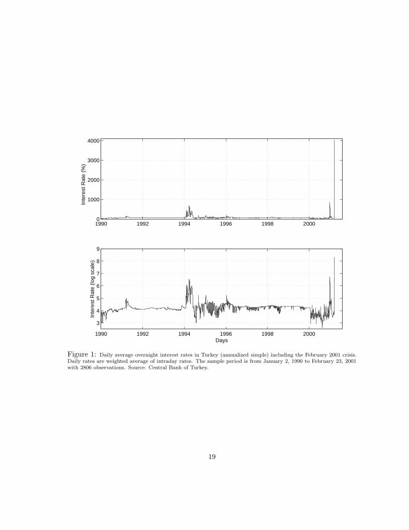
The structure of the stabilization program implied that interest rate would be marketdetermined in line with the exchange rate depreciation and capital flows, and the volatilityof interest rates would be higher than the volatility before the program.3 A close inspectionof Figure 1 reveals that this was the case. After the launch of the program on January 1,2000, the average level of daily overnight interest rates dropped immediately in accord withthe slowed down, fixed depreciation rate, and the volatility of the overnight interest rateincreased.4

During the second half of the year 2000, market participants and foreign investors wereuneasy about developments in the economy. There were several reasons for these concerns.The government was slow in taking action to solve the chronic financial problems of thestate banks and to implement other structural reforms; privatization efforts were not takingplace as planned; some of the ministers in the government raised their voice against the pri-vatization of Turkish Telecom; the current account deficit was increasing to historically high

1See Selcuk (1998) and Ertugrul and Selcuk (2001) for the developments in the Turkish economy in recentyears.

2The net domestic assets of the Central Bank of Turkey are defined as the base money less the net foreignassets of the Central Bank valued at actual exchange rates. The base money is defined as currency issuedby the Central Bank plus the banking sector’s deposits in Turkish Lira with the Central Bank.

3In macroeconomics literature, this situation is known as “an impossible trinity” (a fixed exchange rate,free capital flows and an active monetary policy), i.e., a policy maker cannot fully control both interestrates and exchange rates if capital flows are free in the economy. Since the stabilization program fixed theexchange rate depreciation, and the capital flows were free, there was little room for the Central Bank toaffect interest rates.

4The sample coefficient of variation of the overnight interest rates increased to 0.36 during January 3 -November 17, 2000, from 0.10 which is based on the previous four year sample. The sample coefficient ofvariation is defined as the sample standard deviation divided by the sample mean.

1

levels as a result of the appreciation of the Turkish Lira and negative domestic real interestrates; the relations between Turkey and the European Union started to become very tense;the possibility of closing a major opposition party in the parliament by the constitutionalcourt implied general elections and, finally, Turkey had a history of unsuccessful stand-byarrangements with the IMF. As in many exchange rate-based stabilization programs, cred-ibility appeared to increase in the first phase of the program and, as time passed, inabilityto deal with fundamental problems and an unsound banking system started to erode it.5

It was well-known by the market participants that one of the commercial banks (Demir-bank) had an extremely risky position during the year 2000. The bank (with a paid capitalof USD 300 million) was funding its estimated USD 7.5 billion government securities port-folio mostly from the money market with short term obligations. On Monday, November20, 2000, Demirbank was not able to borrow from the money market and the Central Bankstepped in to cover Demirbank’s position. In the following days, market makers in the gov-ernment securities market stopped posting prices and Demirbank was not able to liquidateits positions. As a result, overnight interest rates started to increase. Meanwhile, a signif-icant portion of foreign creditors withdrew their credit lines to Turkish banks and startedto liquidate their positions out of devaluation fears. Major international investment housesand banks started to recommend “fire sale” to their clients in their bulletins and reports.Suddenly, there was a rapid capital outflow, starting on Wednesday, November 22.6

As a result of the heavy capital outflow and decrease in the Central Bank reserves,liquidity pressure rocketed the interest rates. The Central Bank started to provide liquidityto the market violating the rule set by the stand-by agreement for the net domestic assets.However, the injected liquidity bounced back to the Central Bank in the form of additionaldemand for foreign currency. Therefore, the Central Bank stopped providing liquidity aftersix business days, on Thursday, November 30, 2000. Immediately, the overnight interest ratereached its peak at (simple annual) 873 percent on Friday, December 1, 2000. Total capitaloutflow during this period reached an estimated USD 6 billion, eroding approximately 25percent of the foreign exchange reserves of the Central Bank. Over the weekend, the IMFrushed in an “emergency team” consisting of two delegations to discuss an emergency loan.On Tuesday, December 5, Turkish authorities announced a USD 7.5 billion rescue packagewith the IMF. The following morning before the markets opened, Demirbank became the11th Turkish bank to be taken under control of the Saving Deposits Insurance Fund. Theowner of the Demirbank went on record stating that:

5See Guidotti and Vegh (1999) for a political-economy model that focuses on the evolution of credibilityover time under exchange rate-based stabilization programs.

6Dornbusch (2001) discusses the makings of emerging market crises in general and claims that a largenumber of poorly managed banks and the banking system’s short term funding caused the Turkish financialcrisis in 2000. Stanley Fischer, the first deputy managing director of the IMF, relates the crisis in Turkey tobanking sector problems and the failure to undertake corrective fiscal actions against the widening currentaccount deficit. See Fischer (2001).

2

“Naturally, while buying the treasury bond Demirbank thought interest ratesmight rise and accounted for that. But the rise we are talking about was aboveand beyond logic and reason. No institution could foresee [annualized com-pound] interest rates in thousands, ten thousands or even billions. [R]ates sud-denly became crazy and rose to the levels unseen in the history of the Republic.This situation ripped [us] apart.” Reuters News Service. December 12, 2000.

However, other bankers had a different perspective:

“Around mid-November, Demirbank with a paid capital of USD 300 millionwas carrying a T-bill stock of USD 4-5 billion and it was extremely squeezed.[These] fellows were taking an extremely high risk and this risk cost them theirlives.” Reuters News Service. December 6, 2000.

After the IMF’s backing of the country in December 2000, there was short-term capitalinflow to the economy, especially in the beginning of the year 2001, and the Central Bankreserves returned to its pre-crisis level. Interest rates decreased, albeit stabilizing at a higherlevel than the pre-crisis average. Nevertheless, the market participants were not comfortableabout developments in the economy and there were concerns about the Treasury’s abilityto borrow from the domestic market at favorable terms. A scheduled domestic debt auctionof the Treasury on February 20, 2001, the day before the maturing USD 7 billion domesticdebt aimed at borrowing approximately USD 5 billion (around ten percent of the totaldomestic debt).

Suddenly, on February 19, 2001, the day before the auction, Turkish Prime MinisterBulent Ecevit stormed out of a key meeting of top political and military leaders stating a“dispute” had arisen between himself and the country’s president. He further emphasizedthat “of course, this is a serious political crisis” without elaborating the future of thegovernment or the economic program. The news hit the market and the stock market dived18 percent in one day. The same day, the Central Bank sold USD 7.5 billion (approximatelyone-third of the total official reserves) for the next day delivery to the banks which had yetto recover from the November crisis. The next day, two state banks (Ziraat and Halkbank)were not able to meet their obligations in the markets and the Central Bank refused toprovide Turkish Lira liquidity to the banks.7 Therefore, banks were forced to sell USD 5billion back to the Central Bank. The daily average overnight interest rates rocketed upto (simple annual) 2000 percent on February 20, and 4000 percent on February 21. Thegovernment responded by dropping its exchange-rate controls early February 22 to take thepressure off on rates, and the TL/USD exchange rate went up 40 percent in one week. Oneweek after this second crisis, another bank (Ulusalbank) became the 12th Turkish bank to

7Market sources estimate that the total obligations of two state banks were approximately USD 7 billionon that particular day.

3

be taken under control of the Saving Deposits Insurance Fund. Incidentally, Ulusalbankwas controlled by the same group who used to own Demirbank.

The Turkish financial crisis in February 2001 is a case study for extreme risks and riskmanagement practices. In recent years, the problem of extreme risks in financial marketshas become topical following the recent turmoils in the Asian and Russian markets, andthe unexpected big losses of investment banks such as Barings and Daiwa. The BaselCommittee has set rules to be followed by banks to control their risks, but most of thewell-studied models for assessing risks are based on the assumption that financial assetsare distributed according to a normal distribution. In particular, the value-at-risk (VaR)measures with Gaussian-type innovations failed to cope with the recent turmoils withinthe Asian and Russian markets in market and credit risk computations. In the Gaussianmodel the evaluation of extreme risks is directly related to the variance, but in the case offat-tailed distributions this is not the case since the underlying distribution may not evenhave a finite variance.

In this paper, we investigate the dynamics of the extreme values of overnight borrowingrates in the inter-bank money market before the Turkish financial crisis of February 2001.It is shown that the generalized Pareto distribution model fits well to the tail of the interestrate distribution. We also provide estimates of overnight borrowing rates at 0.999 percentilebefore the crisis. Our findings indicate that the extremely high overnight interest ratesobserved during the February 2001 crisis (up to 4000 percent) emerge as a possible outcomefrom the pre-crisis data, although it has not been observed before.

This paper is structured as follows. In Section 2, the extreme value theory with ref-erence to the Fisher-Tippett framework, the generalized Pareto distribution (GPD), thetail estimation, and the tools used in the preliminary data analysis for the extreme valuetheory applications are presented. Section 3 reports the descriptive statistics, the maximumlikelihood estimation of the GPD parameters for the overnight interest rates and other em-pirical results. Since the Turkish daily overnight rates has not been studied widely in theliterature and is not well known, we also study the daily U.S. Effective Federal Funds Rateas a benchmark comparison. We conclude afterwards.

2. Extreme Value Theory

From the practitioners’ point of view, one of the most interesting questions that tail studiescan answer is what are the extreme movements that can be expected in financial markets?Have we already seen the largest ones or are we going to experience even larger movements?Are there theoretical processes that can model the type of fat tails that come out of ourempirical analysis? Answers to such questions are essential for sound risk management offinancial exposures. It turns out that we can answer these questions within the frameworkof the extreme value theory. Once we know the tail index, we can extend the analysis

4

outside the sample to consider possible extreme movements that have not yet been ob-served historically. This can be achieved by computation of the quantiles with exceedanceprobabilities.

Evidence of heavy tails in financial asset returns is plentiful (Koedijk et al, 1990; Holsand de Vries, 1991; Loretan and Phillips, 1994; Ghose and Kroner, 1995; Danielsson andde Vries, 1997; Muller et al. 1998; Pictet et al. 1998; Hauksson et al. 2000; Dacorognaet al. 2001a,b) since the seminal work of Mandelbrot on cotton prices (Mandelbrot, 1963).Mandelbrot advanced the hypothesis of a stable distribution on the basis of an observedinvariance of the return distribution across different frequencies and apparent heavy tailsin return distributions. A continuing controversy has long been in the financial research asto whether the second moment of the returns converges. This question is central to manymodels in finance, which rely heavily on the finiteness of the variance of returns.

Extreme value theory is a powerful and yet fairly robust framework to study the tailbehavior of a distribution. Embrechts et al. (1997) is a comprehensive source of the extremevalue theory to the finance and insurance literature. Reiss and Thomas (1997) and Beirlantet al. (1996) also have extensive coverages on the extreme value theory.

Although the extreme value theory has found large applicability in climatology and hy-drology8, there have been a number of extreme value studies in finance literature in therecent years. De Haan et al. (1994) study the quantile estimation using the extreme valuetheory. McNeil (1997, 1998) study the estimation of the tails of loss severity distributionsand the estimation of the quantile risk measures for financial time series using extreme valuetheory. Embrechts et al. (1998) overviews the extreme value theory as a risk managementtool. Muller et al. (1998) and Pictet et al. (1998) study the probability of exceedancesfor the foreign exchange rates and compare them with the GARCH and HARCH models.Embrechts (1999, 2000) study the potentials and limitations of the extreme value theory.McNeil (1999) provides an extensive overview of the extreme value theory for risk managers.McNeil and Frey (2000) studies the estimation of tail-related risk measures for heteroskedas-tic financial time series. In the following section, we present the parametric framework forour study.

2.1. Fisher-Tippett Theorem

The normal distribution is the important limiting distribution for sample sums or averagesas summarized in a central limit theorem. Similarly, the family of extreme value distribu-tions are the ones to study the limiting distributions of the sample maxima. This family canbe presented under a single parameterization known as the generalized extreme value distri-bution (GEV). The theorem of Fisher and Tippett (1928) is in the core of the extreme value

8Embrechts et al. (1997) has a large collection of literature in applications of the extreme value theoryin other fields.

5

theory. The theory deals with the convergence of maxima. Suppose that x1, x2, . . . , xm is asequence of independently and identically distributed9 random variables from an unknowndistribution function F (x) where x ∼ (µ, σ2) and m is the sample size. Denote the maxi-mum of the first n < m observations of x by Mn = max(x1, x2, . . . xn). Given a sequenceof an > 0 and bn such that (Mn − bn)/an, the sequence of normalized maxima converges inthe following GEV distribution

H(x) =

e−(1+ξ x

β

)−1/ξ

if ξ �= 0

e−e−x/βif ξ = 0,

(1)

where β > 0 and x is such that 1+ ξx > 0 and ξ is the shape parameter.10 When ξ > 0, thedistribution is known as the Frechet distribution and it has a fat-tail. The larger the shapeparameter, the more fat-tailed the distribution. If ξ < 0, the distribution is known as theWeibull distribution. Finally, if ξ = 0, it is the Gumbel distribution.11 The Fisher-Tippetttheorem suggests that the asymptotic distribution of the maxima belongs to one of the threedistributions above, regardless of the original distribution of the observed data. Therefore,the tail behavior of the data series can be estimated from one of these three distributions.

The class of distributions of F (x) where the Fisher-Tippett theorem holds is quitelarge.12 One of the conditions is that F (x) has to be in the domain of attraction for theFrechet distribution13 (ξ > 0) which in general holds for the financial time series. Gnedenko(1943) shows that if the tail of F (x) decays like a power function, then it is in the domainof attraction for the Frechet distribution. The class of distributions whose tails decaylike a power function are large and include the Pareto, Cauchy, Student-t and mixturedistributions. These distributions are the well-known heavy tailed distributions.

The distributions in the domain of attraction of the Weibull distribution (ξ < 0) are theshort tailed distributions such as uniform and beta distributions which do not have muchpower in explaining financial time series. The distributions in the domain of attraction ofthe Gumbel distribution (ξ = 0) include the normal, exponential, gamma and lognormaldistributions where only the lognormal distribution has a moderately heavy tail.

9The assumption of independence can be easily dropped and the theoretical results follow through (seeMcNeil 1997). The assumption of identical distribution is for convenience and can also be relaxed.

10The tail index is defined as α = ξ−1.11An extensive coverage can be found in Gumbel (1958).12McNeil (1997, 1999), Embrechts et al. (1997, 1998) and Embrechts (1999) have excellent discussions of

the theory behind the extreme value distributions from the risk management perspective.13See Falk et al. (1994).

6

2.2. Generalized Pareto Distribution

In general, we are not only interested in the maxima of observations, but also in the be-havior of large observations which exceed a high threshold. Given a high threshold u, thedistribution of excess values of x over threshold u is defined by

Fu(y) = Pr{X − u ≤ y|X > u} =F (y + u) − F (u)

1 − F (u). (2)

which represents the probability that the value of x exceeds the threshold u by at most anamount y given that x exceeds the threshold u. A theorem by Balkema and de Haan (1974)and Pickands (1975) shows that for sufficiently high threshold u, the distribution functionof the excess may be approximated by the generalized Pareto distribution (GPD) such that,as the threshold gets large, the excess distribution Fu(y) converges to the GPD which is

G(x) =

1 −

(1 + ξ x

β

)−1/ξif ξ �= 0

1 − e−x/β if ξ = 0,

(3)

where ξ is the shape parameter. The GPD embeds a number of other distributions. Whenξ > 0, it takes the form of the ordinary Pareto distribution. This particular case is the mostrelevant for financial time series analysis since it is a heavy tailed one. For ξ > 0, E[Xk]is infinite for k ≥ 1/ξ. For instance, the GPD has an infinite variance for ξ = 0.5 and,when ξ = 0.25, it has an infinite fourth moment. For the security returns or high frequencyforeign exchange returns, the estimates of ξ are usually less than 0.5, implying that thereturns have finite variance (Jansen and deVries 1991, Longin 1996, Muller et al. 1996, andDacorogna et al. 2001b). When ξ = 0, the GPD corresponds to exponential distributionand it is known as a Pareto II type distribution for ξ < 0.

The importance of the Balkema and de Haan (1974) and Pickand (1975) results is thatthe distribution of excesses may be approximated by the GPD by choosing ξ and β andsetting a high threshold u. The GPD can be estimated with various methods such asthe method of probability weighted moments or the maximum likelihood method.14 Forξ > −0.5 which corresponds to heavy tails, Hosking and Wallis (1987) presents evidencethat maximum likelihood regularity conditions are fulfilled and the maximum likelihoodestimates are asymptotically normally distributed. Therefore, the approximate standarderrors for the estimators of β and ξ can be obtained through maximum likelihood estimation.

14Hosking and Wallis (1987) has discussions on the comparisons between various methods of estimation.

7

2.3. The Tail Estimation

The conditional probability in previous section is

Fu(y) =Pr{X − u ≤ y,X > u}

Pr(X > u)=

F (y + u) − F (u)1 − F (u)

. (4)

Since x = y + u for X > u, we have the following representation

F (x) = [1 − F (u)] Fu(y) + F (u). (5)

Notice that this representation is valid only for x > u. Since Fu(y) converges to the GPDfor sufficiently large u, and since x = y + u for X > u, we have

F (x) = [1 − F (u)] Gξ,β,u(x − u) + F (u). (6)

For a high threshold u, the last term on the right hand side can be determined by theempirical estimator (n−Nu)/n where Nu is the number of exceedances and n is the samplesize. The tail estimator, therefore, is given by

F (x) = 1 − Nu

n

(1 + ξ

x − u

β

)−1/ξ

. (7)

For a given probability q > F (q), a percentile (xq) at the tail is estimated by inverting thetail estimator in Equation 7,

xq = u +β

ξ

((n

Nu(1 − q)

)−ξ

− 1

). (8)

In statistics, this is the quantile estimation and it is the Value-at-Risk (VaR) in the financeliterature.

2.4. Preliminary Data Analysis

In statistics, a QQ-plot (quantile-quantile plot) is a convenient visual tool to examinewhether a sample comes from a specific distribution. Specifically, the quantiles of a hy-pothesized distribution are plotted against the quantiles of an empirical distribution. If thesample comes from the hypothesized distribution, the QQ-plot is linear. In the extremevalue theory and applications, the QQ-plot is typically plotted against the exponentialdistribution (i.e, a distribution with a thin-sized tail) to measure the fat-tailness of a dis-tribution. If the data is from an exponential distribution, the points on the graph wouldlie along a positively sloped straight line. If there is a concave presence, this would indi-cate a fat-tailed distribution, whereas a convex departure is an indication of short-taileddistribution.

8

A second tool is the sample mean excess function (MEF) which is defined by

en(u) =∑n

i=1(Xi − u)∑ni=1 I{Xi>u}

. (9)

where I is an indicator function. The MEF is the sum of the excesses over the thresholdu divided by the number of data points which exceed the threshold u. It is an estimateof the mean excess function which describes the expected overshoot of a threshold oncean exceedance occurs. If the empirical MEF is a positively sloped straight line above acertain threshold u, it is an indication that the data follows the GPD with a positive shapeparameter ξ. On the other hand, exponentially distributed data would show a horizontalMEF while short tailed data would have a negatively sloped line.

Another tool in threshold determination is the Hill-plot.15 Hill (1975) proposed thefollowing estimator for ξ

ξ =1

k − 1

k−1∑i=1

ln Xi,N − ln Xk,N for k ≥ 2 (10)

where k is upper order statistics (the number of exceedances), N is the sample size, andα = 1/ξ is the tail index. A Hill-plot is constructed such that estimated ξ is plotted as afunction of k upper order statistics (at lower horizontal axis) and of the threshold (at theupper horizontal axis). A threshold is selected from the plot where the shape parameter ξ

is fairly stable.In threshold determination, we face a trade off between bias and variance. If we choose

a low threshold, the number of observations (exceedances) increases and the estimationbecomes more precise. However, choosing a low threshold also introduces some observationsfrom the center of the distribution and the estimation becomes biased. Therefore, a carefulcombination of several techniques, such as the QQ-plot, the Hill-plot and the MEF shouldbe considered in threshold determination.

3. Empirical results

The data source for the daily overnight interest rates (simple annual) is the Central Bankof Turkey. The daily rates are calculated by the Central Bank as a weighted average ofintraday transactions in the interbank money market.16 The descriptive statistics of dailyaverage simple annual overnight interest rates before and after the February 2001 crisis aregiven in Table 1. The full sample period is January 2, 1990 - February 23, 2001 with 2806

15See Embrechts, et al. (1997, Chapter 6) for a detailed discussion and several examples of the Hill-plot.16The observed maximum intraday interest rate is (simple annual) 8000 percent. This means borrowing

Turkish Lira at an interest rate of 22.2 percent for one day (22.2 ∗ 360 ≈ 8000).

9

observations. It includes all available daily interest rate data from the inter-bank moneymarket in Turkey. In this paper, all calculations and predictions are carried out with simpleannual interest rates.

In Table 1, the sample means of 73.0 and 75.7 percent correspond to compound annualinterest rates of approximately 107 and 113 percent, respectively.17 Although it is highby the standards of a developed market, it reflects the high inflation levels and associatedrisk in the economy. The annual average percent increase in consumer prices (inflation)during the sample period was 75.4 percent, implying an average annual real interest rateof 18-21 percent.18 Both kurtosis and skewness estimates show that the interest rates arefar from being normally distributed. The estimated kurtosis 82.62 before the crisis showsthat the interest rate distribution has a fat tail. The estimated skewness of 7.5 before thecrisis points out that the distribution is skewed. After the crisis, both skewness (26.4) andkurtosis (943.2) estimates indicate that fat-tailness and skewness of the distribution havesubstantially increased.

3.1. Tail Estimation of Excess Interest Rates

It is necessary to determine a threshold interest rate to estimate the parameters of thegeneralized Pareto (GPD) distribution. As presented in Section 2.4, the QQ-plot and themean excess function are two empirical tools for this task. In a QQ-plot, the quantilesof the empirical distribution function on the x-axis are plotted against the quantiles ofthe exponential distribution function on the y-axis. The points should lie approximatelyalong a straight line if the data is from an exponential distribution. Since the exponentialdistribution has a medium-sized tail, a concave relationship between the quantiles of theempirical and exponential distributions indicate a heavy-tailed distribution for the timeseries under study. The top panel of Figure 2 indicates that the sample points start deviatingfrom linear behavior at around 80 percent and form a concave pattern.

The sample mean excess function is another diagnostic tool to determine a threshold.If the points of the mean excess function exhibit an upward trend, this indicates heavy-tailed behavior. Short-tailed data exhibit negatively sloped behavior whereas an exponential

17The annual compound interest rate is calculated by

1 + cr = [1 + (sr/360)]360

where cr is annual compound interest rate and sr is annual simple interest rate. FX and money market daysbasis is 360 whereas capital markets days basis is 365 in the Turkish markets.

18It is a common practice among researchers and practitioners in developed economies to calculate thereal interest rate as “nominal rate minus inflation”. This approximation holds only for low levels of inflation.The exact formula for the real interest rate calculation is 1 + r = 1+i

1+πwhere r is the real interest rate, i is

the nominal rate and π is the corresponding inflation rate. In our calculations of the average annual realinterest rate, i is the nominal annual compound interest rate and π is the annual inflation rate.

10

distribution has a flat mean excess function. The bottom panel of Figure 2 demonstratesthat the sample mean excess function is approximately linear and positively sloped afterthe 80 percent interest rate threshold. The examination of both panels in Figure 2 indicatethat the approximate threshold value corresponds to 80 percent.

For a given threshold level, a tail estimation involves the estimation of the parametersof the generalized Pareto distribution. The maximum likelihood estimation is a convenientway to obtain standard errors of the parameter estimates.19 For the threshold u = 80, thethreshold exceedances are 389 data points which constitute the upper 13.9 percent tail ofthe original sample of 2801 sample points. Notice that an 80 percent overnight interestrate (simple annual) is equivalent to an annualized compound interest rate of 122 percent.During the sample period, the average annual percent increase in TL/USD exchange rateis 75 percent. Therefore, the threshold implies a 23 percent annualized dollar interest rate.

The maximum likelihood estimate of ξ and β at threshold u = 80 are (standard errorsare in parenthesis) 0.73 (0.086) and 22 (2.03), respectively. The estimated parameters arestatistically significant at the 1 percent level. As discussed in Section 2.1, when ξ > 0, thedistribution is known as the Frechet distribution and it has a fat-tail. The larger the shapeparameter, the more fat-tailed the distribution. The value of ξ = 0.73 indicates that theovernight interest rate series come from a fat-tail distribution with infinite variance.

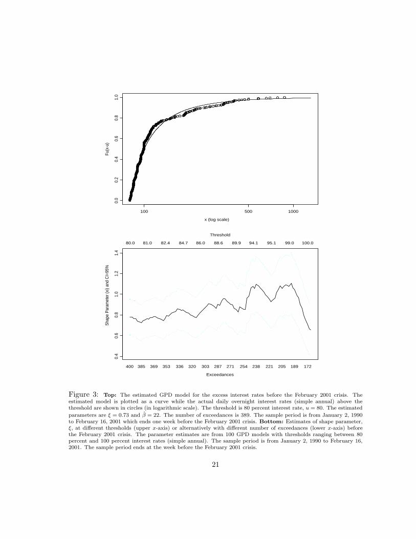
The estimated GPD model with a threshold 80 percent interest rate (u = 0.80) with theinterest rate data before the February 2001 crisis is presented in the top panel of Figure 3.The estimated model is plotted in a solid curve while the interest rates above the thresholdare shown in circles (on logarithmic scale). The estimated model successfully capturesthe underlying extreme values, and the tail behavior of excess interest rates is successfullyapproximated by a Frechet-type distribution.

To examine the robustness of the results to the choice of the threshold value, the maxi-mum likelihood estimation of the shape parameter, ξ, is carried out for GPD models with arange of thresholds between 80 to 100 percent. The estimates of ξ, as well as their asymp-totic confidence intervals, are reported in the bottom panel of Figure 3. On the lower x-axisthe number of data points exceeding the threshold is plotted and on the upper x-axis thethreshold is located. The estimates of the shape parameter, ξ, are plotted on the y-axis.The results indicate that the shape parameter exhibits a stable but upward sloping pathconfirming the thick-tailness of the data. Of course, there are fewer observations at higherthresholds and less statistical precision. This is reflected in the wider confidence intervalsaround the threshold value of 100.

19EVIS (Extreme Values in S-Plus) is a free S-Plus functions for EVT. The package may be obtained fromhttp://www.math.ethz.ch/∼mcneil.

11

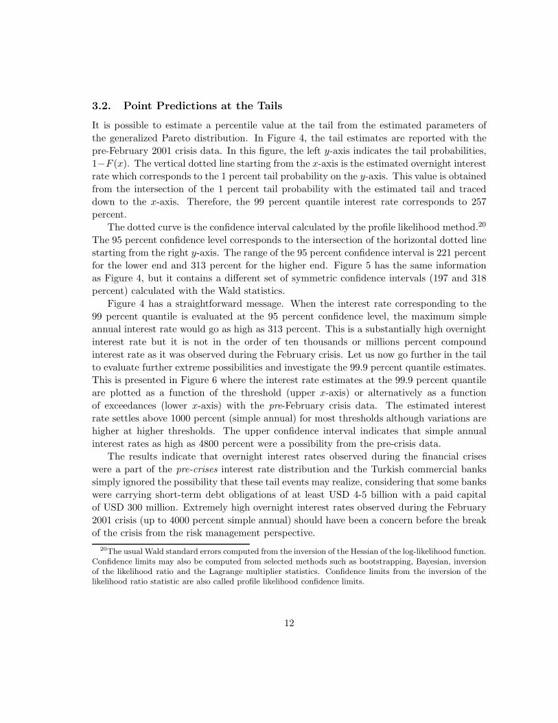
3.2. Point Predictions at the Tails

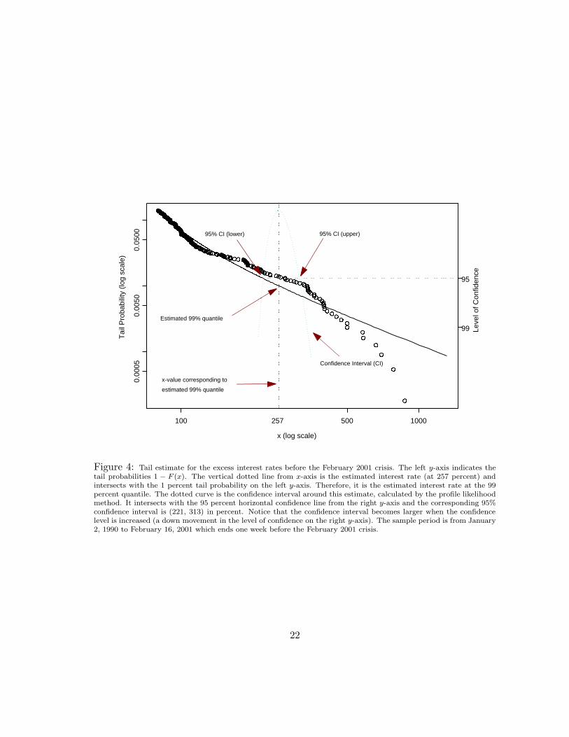
It is possible to estimate a percentile value at the tail from the estimated parameters ofthe generalized Pareto distribution. In Figure 4, the tail estimates are reported with thepre-February 2001 crisis data. In this figure, the left y-axis indicates the tail probabilities,1−F (x). The vertical dotted line starting from the x-axis is the estimated overnight interestrate which corresponds to the 1 percent tail probability on the y-axis. This value is obtainedfrom the intersection of the 1 percent tail probability with the estimated tail and traceddown to the x-axis. Therefore, the 99 percent quantile interest rate corresponds to 257percent.

The dotted curve is the confidence interval calculated by the profile likelihood method.20

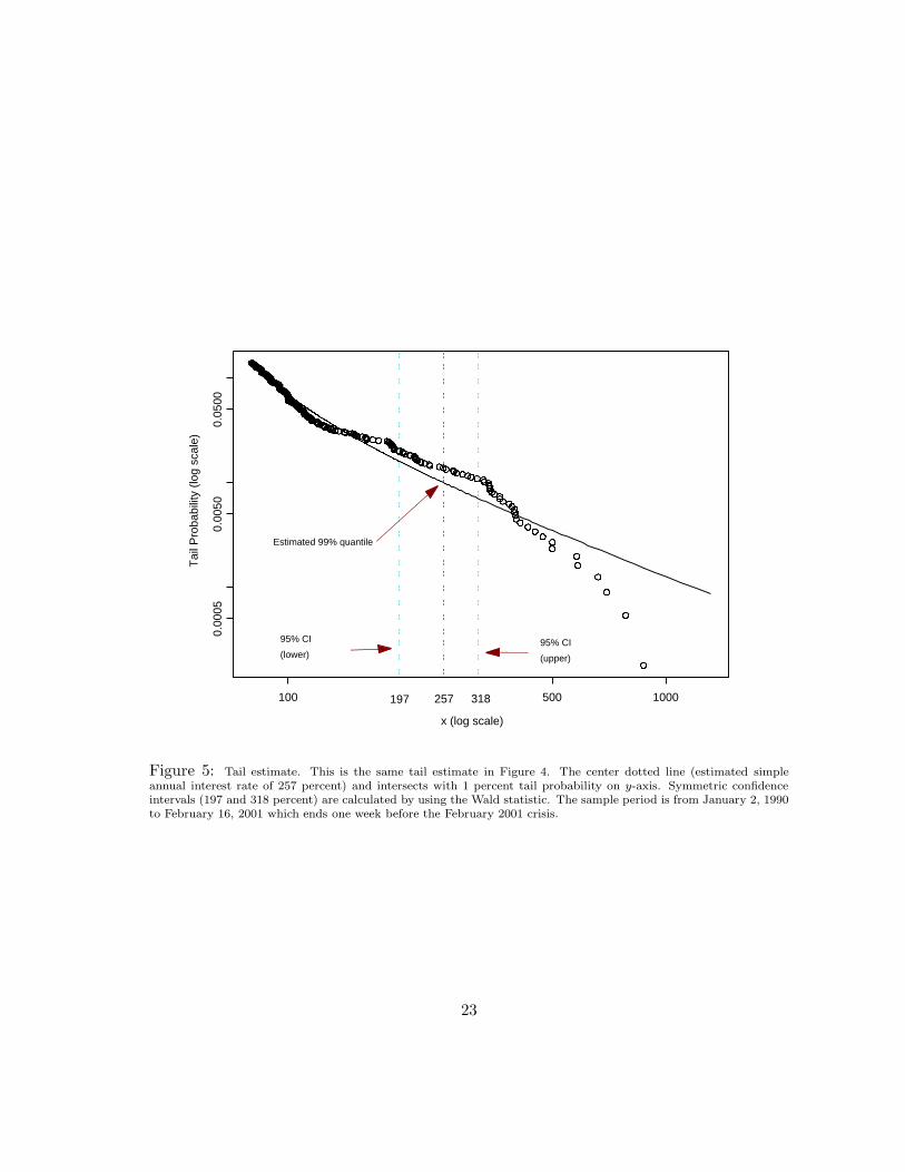
The 95 percent confidence level corresponds to the intersection of the horizontal dotted linestarting from the right y-axis. The range of the 95 percent confidence interval is 221 percentfor the lower end and 313 percent for the higher end. Figure 5 has the same informationas Figure 4, but it contains a different set of symmetric confidence intervals (197 and 318percent) calculated with the Wald statistics.

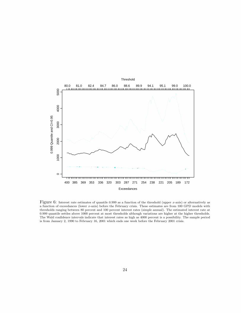
Figure 4 has a straightforward message. When the interest rate corresponding to the99 percent quantile is evaluated at the 95 percent confidence level, the maximum simpleannual interest rate would go as high as 313 percent. This is a substantially high overnightinterest rate but it is not in the order of ten thousands or millions percent compoundinterest rate as it was observed during the February crisis. Let us now go further in the tailto evaluate further extreme possibilities and investigate the 99.9 percent quantile estimates.This is presented in Figure 6 where the interest rate estimates at the 99.9 percent quantileare plotted as a function of the threshold (upper x-axis) or alternatively as a functionof exceedances (lower x-axis) with the pre-February crisis data. The estimated interestrate settles above 1000 percent (simple annual) for most thresholds although variations arehigher at higher thresholds. The upper confidence interval indicates that simple annualinterest rates as high as 4800 percent were a possibility from the pre-crisis data.

The results indicate that overnight interest rates observed during the financial criseswere a part of the pre-crises interest rate distribution and the Turkish commercial bankssimply ignored the possibility that these tail events may realize, considering that some bankswere carrying short-term debt obligations of at least USD 4-5 billion with a paid capitalof USD 300 million. Extremely high overnight interest rates observed during the February2001 crisis (up to 4000 percent simple annual) should have been a concern before the breakof the crisis from the risk management perspective.

20The usual Wald standard errors computed from the inversion of the Hessian of the log-likelihood function.Confidence limits may also be computed from selected methods such as bootstrapping, Bayesian, inversionof the likelihood ratio and the Lagrange multiplier statistics. Confidence limits from the inversion of thelikelihood ratio statistic are also called profile likelihood confidence limits.

12

3.3. A Comparison with the U.S. Interest Rates

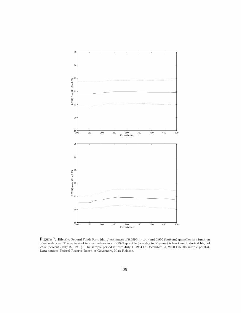
Although the Turkish daily overnight rate is an excellent case study with high volatility anda thick-tailed distribution, this data set has not been studied widely in the literature andis not well known. Hence, we have repeated the extreme value analysis with the the dailyU.S. Effective Federal Funds Rate as a benchmark comparison.21 The GPD estimationswith different numbers of exceedances in this data set indicate that the estimated shapeparameter ξ is remarkably stable around -0.40, corresponding to a Pareto II type distributionwhich is a thin tailed distribution with a finite tail. Figure 7 plots estimated interest ratesfor 0.9999th quantile (one day in every ten thousand days, approximately 30 years), and0.999th quantile (one day in every one thousand days, approximately 3 years) as a functionof the number of exceedances. The estimated interest rate is very stable around 20.5 percentat 0.1% tail and at around 22 percent at 0.01% tail regardless of the number of exceedances.Moving in the tail of the distribution from 0.1% to the 0.01% region increases the estimatedinterest rate by only around 150 bases points (one and a half percentage point). Theseestimates imply that the daily effective Federal Funds Rate has an upper bound and it isextremely unlikely to observe an overnight interest rate of, say, 30 percent in the U.S.

4. Lessons from the Turkish Crises and Conclusions

Financial crises in emerging markets in general and the Turkish crises in November 2000and February 2001 in particular provide several lessons for investors both in developingand developed countries. As one prominent economist puts it, “crises are not just financialexperiences but rather involve large and lasting social costs and important redistributionof income and wealth” (Dornbusch, 2001). Since a significant portion of total savings indeveloped economies are invested in emerging markets by hedge funds, mutual funds, andother institutions in the form of portfolio investment, the costs of financial crises are notconfined with the residents of emerging market countries.22 Therefore, a careful investi-gation of the market dynamics and the causes of crises in these economies would benefitinvestors at large by increasing the investor awareness.23

Fundamental macroeconomic indicators such as growth rate, current account balance,real exchange rate, budget deficit, export-import ratio, debt-income ratio are the main

21The sample period is from July 1, 1954 to December 31, 2000. The sample size is 16,986 daily observa-tions. Data source: Federal Reserve Board of Governors, H.15 release.

22Although there is a substantial decrease in recent years, the net portfolio investment in emerging marketsby other countries in one year was USD 58.3 billion in 2000. The historical record is USD 109.9 billion in1994. Source: IMF, International Financial Statistics.

23Foreign investors may face completely different financial circumstances in emerging economies than theyhave in their home country. To point out this, Dornbusch (2001) refers to the catchy title of an article writtenin the early 1980s about the debt crisis in Latin American economies: “We are not in Kansas anymore..”(Diaz Alejandro, 1984).

13

source of assessing the current and future status of an economy. Therefore, they play asignificant role in decision making process of credit rating agencies and in portfolio allocationdecision of multinational fund managers. One of the lessons from the Turkish crisis is thateven if there is no deterioration in fundamental macroeconomic indicators, the balance sheetissues in the finance sector may create an environment in which even a small shock can leadto a total collapse of the system. Especially, a balance sheet mismatch situation (fundinglong-term illiquid assets with short-term obligations) combined with slack supervision andregulation is an invitation for liquidity and currency crisis. Among others, Eichengreen(2001) investigates both Argentinian and Turkish crisis in detail. He points out to thevulnerability of the banking sector to be the main source of crisis in Turkey.24

According to a real exchange rate index recently published by the Turkish CentralBank, the lira appreciated 37 percent between January 1995 and January 2000, the monththe stabilization program started. Nevertheless, the Turkish stabilization program adopteda crawling peg to reduce inflation by limiting the lira’s devaluation to 15 percent per year.Although it was expected that the lira was going to appreciate further during the program,the government could not commit to an upfront devaluation as the Turkish banks andthe private sector had accumulated large unhedged foreign exchange exposures during thepast 5-6 years. It was hoped by the program designers that the banking sector wouldstrengthen before the economy would move into a floating exchange rate regime after 18months. As Eichengreen (2001) points out, this strategy created a moral hazard in thesystem and the incentive to strengthen both balance sheets and supervision diminished.25

As a result, short foreign exchange positions of the banks doubled during the first ninemonths of the program. The direct consequence of this was that the fear of destabilizingthe economy forced the authorities to resist any correction in the exchange rate, even if itmeant extraordinary increases in overnight interest rates.26 Given the governments strongcommitment to exchange rates, the relevant question from the investors’ point of view was“what extraordinary interest rates may be observed under extreme situations?”. Our resultsat 99.9 percent quantile show that 2000-4800 percent interest rates (simple annual) were apossibility in the economy, although it had not been observed before.

24See Dooley and Frankel (2001) for a collection of studies on currency crises in different emerging marketeconomies.

25According to Eichengreen (2001), the moral hazard was created “because exchange risk was socialized,that is to say, its strategy committed the government to preventing the exchange rate from moving andtherefore to compensating the banks for their losses if the policy failed”.

26See Calvo and Reinhart (1999) on the fear of floating the exchange rate in emerging economies.

14

References

[1] Balkema, A. A. and L. de Haan (1974), Residual lifetime at great age, Annals of Probability, 2,792–804.

[2] Beirlant, J., J. Teugels, and P. Vynckier (1996), Practical Analysis of Extreme Values, LeuvenUniversity Press, Leuven.

[3] Calvo, G.A. and C. M. Reinhart (2000), Fear of floating, manuscript, Department of Economics,University of Maryland, College Park, Maryland.

[4] Dacorogna, M. M., O. V. Pictet, U. A. Muller, and C. G. de Vries (2001a), Extremal forexreturns in extremely large data sets, Extremes, forthcoming.

[5] Dacorogna, M. M., R. Gencay, U. A. Muller, R. B. Olsen and O. V. Pictet (2001b), An Intro-duction to High Frequency Finance, Academic Press, San Diego.

[6] Danielsson, J and C. G. de Vries (1997), Tail index and quantile estimation with very highfrequency data, Journal of Empirical Finance, 4, 241–257.

[7] De Haan, L., D. W. Janssen, K. G. Koedjik and C. G. de Vries (1994), Safety first portfo-lio selection, extreme value theory and long run asset risks, in “Extreme Value Theory andApplications”, J. Galambos, J. Lechner and E. Simiu (eds.), Kluwer, Dordrecht, 471-488.

[8] Diaz Alejandro, C. (1984),“Latin American debt: I don’t think we are in Kansas anymore”,Brookings Papers on Economic Activity, 2, 335–389.

[9] Dooley, M. and J. Frankel (2001), Managing Currency Crises in Emerging Markets (eds.),NBER and The University of Chicago Press, Chicago, forthcoming.

[10] Dornbusch, R. (2001), A primer on emerging market crisis, manuscript, MIT, Department ofEconomics.

[11] Eichengreen, B (2001) “Crisis prevention and management: Any new lessons from Argentinaand Turkey?” Background paper written for the World Bank’s Global Development Finance2002, Economics Department, University of California, Berkeley, CA.

[12] Embrechts, P. (2000), Extremes and Integrated Risk Management, Risk Books and UBS War-burg, London.

[13] Embrechts, P. (1999) Extreme value theory in finance and insurance, manuscript. Departmentof Mathematics, ETH, Swiss Federal Technical University.

[14] Embrechts, P., C. Kluppelberg and T. Mikosch (1997), Modeling Extremal Events for Insuranceand Finance, Springer, Berlin.

[15] Embrechts, P., S. I. Resnick, and G. Samorodnitsky (1998), Extreme value theory as a riskmanagement tool, manuscript, Department of Mathematics, ETH, Swiss Federal TechnicalUniversity.

[16] Ertugrul, A. and F. Selcuk (2001) A brief account of the Turkish economy: 1980-2000,manuscript, Department of Economics, Bilkent University, Ankara.

15

[17] Falk, M., J. Husler and R. Reiss (1994), Laws of Small Numbers: Extremes and Rare Events,Birkhauser, Basel.

[18] Fisher, R. A. and L. H. C. Tippett (1928), Limiting forms of the frequency distribution of thelargest or smallest member of a sample, Proceeding of Cambridge Philoshophical Society, 24,180-190.

[19] Fischer, S. (2001), Exchange rate regimes: Is the bipolar view correct?, manuscript, Interna-tional Monetary Fund.

[20] Ghose, D., and K. F. Kroner (1995), The relationship between GARCH and symmetric stableprocesses: Finding the source of fat tails in financial data, Journal of Empirical Finance, 2,225–251.

[21] Gnedenko , B. (1943), Sur la distribution limite du terme maximum d’une serie aleatoire, Annalsof Mathematics, 44, 423-453.

[22] Guidotti, P. E and C. A. Vegh (1999), Losing credibility: The stabilization blues, InternationalEconomic Review, (40), 1, 23–51.

[23] Gumbel, E. (1958), Statistics of Extremes, Colombia University Press, New York.

[24] Hauksson, H. A., M. Dacorogna, T. Domenig, U. Muller, and G. Samorodnitsky (2000), Multi-variate extremes, aggregation and risk estimation, manuscript, School of Operations Researchand Industrial Engineering, Cornell University.

[25] Hill, B. M. (1975), A simple general approach to inference about the tail of a distribution,Annals of Statistics, 3, 1163–1174.

[26] Hols, M. C., and C. G. de Vries (1991), The limiting distribution of extremal exchange ratereturns, Journal of Applied Econometrics, 6, 287–302.

[27] Hosking, J. R. M. and J. R. Wallis (1987), Parameter and quantile estimation for the generalizedPareto distribution, Technometrics, 29, 339–349.

[28] Jansen, D. and C. G. de Vries (1995), On the frequency of large stock returns: Putting boomsand busts into perspective, The Review of Economics and Statistics, 82, 619–631.

[29] Koedijk, K. G., M. M. A. Schafgans and C. G. de Vries (1990), The tail index of exchange ratereturns, Journal of International Economics, 29, 93–108.

[30] Longin, F. (1996), The Asymptotic distribution of extreme stock market returns, Journal ofBusiness, 63, 383–408.

[31] Loretan, M., and P. C. B. Phillips (1994), Testing the covariance stationarity of heavy-tailedtime series, Journal of Empirical Finance, 1, 211–248.

[32] Mandelbrot, B. B. (1963), The variation of certain speculative prices, Journal of Business, 36,394–419.

[33] McNeil, A. J. (1997), Estimating the tails of loss severity distributions using extreme valuetheory, ASTIN Bulletin, 27, 117–137.

16

[34] McNeil, A. J. (1998), Calculating quantile risk measures for financial time series using ex-treme value theory, manuscript, Department of Mathematics, ETH, Swiss Federal TechnicalUniversity.

[35] McNeil, A. J. (1999), Extreme value theory for risk managers, in Internal Modeling and CADII, Risk Books, 93–113.

[36] McNeil A. J. and R. Frey (2000), Estimation of tail-related risk measures for heteroscedasticfinancial time series: An extreme value approach, Journal of Empirical Finance, 7, 271-300.

[37] Muller, U. A, M. M. Dacorogna, O. V. Pictet (1996), Heavy tails in high frequency financialdata, Olsen & Associates Discussion Paper.

[38] Muller, U. A., M. M. Dacorogna, and O. V. Pictet (1998), Heavy tails in high-frequency financialdata, in “A Practical Guide to Heavy Tails: Statistical Techniques for Analysing Heavy TailedDistributions”, R. J. Adler, R. E. Feldman and M. S. Taqqu (eds.), pp. 55–77, Birkhauser,Boston, MA.

[39] Pickands, J. (1975), Statistical inference using extreme order statistics, Annals of Statistics, 3,119–131.

[40] Pictet, O. V., M. M. Dacorogna, and U. A. Muller (1998), Hill, bootstrap and jackknife estima-tors for heavy tails, in “A practical guide to heavy tails: Statistical Techniques for AnalysingHeavy Tailed Distributions”, R. J. Adler, R. E. Feldman and M. S. Taqqu, (eds.), pp. 283-310,Birkhauser, Boston, MA.

[41] Reiss, R. and M. Thomas (1997), Statistical Analysis of Extreme Values, Birkhauser, Basel.

[42] Reuters (2000), Turk Demirbank owner says victim of IMF plan, Reuters News Service, byOsman Senkul, December 6, 2000.

[43] Reuters (2000), Analysis: How bankers view the crisis and its effects, Reuters News Service, byServet Yildirim (in Turkish), December 12, 2000.

[44] Selcuk, F. (1998), A brief account of the Turkish economy, 1987-1996, in “The Political Economyof Turkey in the Post-Soviet Era: Going West and Looking East”, Rittenberg, Libby (ed.),Connecticut: Praeger Publishers.

17

N Mean Std. Ku. Sk. Med. Min. Max. Low High

Pre-crisis 2801 73.0 49.4 82.62 7.5 67.7 13.6 873.1 34.0 107.7

Full Sample 2806 75.7 99.6 943.2 26.4 67.7 13.6 4018.6 34.4 109.6

Table 1: Descriptive statistics of the (simple annual) overnight interest rates before and after crisis. N: samplesize; Mean: Sample mean; Std: Standard deviation; Ku: Kurtosis; Sk: Skewness; Min: Minimum observed rate; Max:Maximum observed rate; Low: Rate corresponding to 5th percentile; High: Rate corresponding to 95th percentile.Full sample period is from January 2, 1990 to February 23, 2001 with 2806 observations. Pre-crisis period excludesthe last five business days. Source: Central Bank of Turkey. Overnight interest rates are daily weighted average ofinter-bank interest rates as calculated by the Central Bank of Turkey.

18

1990 1992 1994 1996 1998 20000

1000

2000

3000

4000

Inte

rest

Rat

e (%

)

1990 1992 1994 1996 1998 2000

3

4

5

6

7

8

9

Inte

rest

Rat

e (lo

g sc

ale)

Days

Figure 1: Daily average overnight interest rates in Turkey (annualized simple) including the February 2001 crisis.Daily rates are weighted average of intraday rates. The sample period is from January 2, 1990 to February 23, 2001with 2806 observations. Source: Central Bank of Turkey.

19

0 200 400 600 800

02

46

8

Ordered Data

Expo

nent

ial Q

uant

iles

20 40 60 80 100 120

2040

6080

100

120

140

Threshold

Mea

n Ex

cess

Figure 2: Top: QQ-plot of daily overnight interest rates (simple annual) before the February 2001 crisis againstthe exponential distribution. The quantiles of the empirical distribution function on the x-axis are plotted againstthe quantiles of the exponential distribution function on the y-axis. The points should lie along the straight line ifthe data is from an exponential distribution. A concave presence indicates a fat-tailed distribution. Source: CentralBank of Turkey. Bottom: Sample mean excesses of daily overnight interest rates (simple annual) before the February2001 crisis over increasing thresholds. A straight line with positive slope above a given threshold u is a sign of theGPD in tail. Notice that the plot is approximately linear and positively sloped after 80 percent, indicating the Paretobehavior in the tail.

20

100 500 1000

0.0

0.2

0.4

0.6

0.8

1.0

x (log scale)

Fu(x

-u)

400 385 369 353 336 320 303 287 271 254 238 221 205 189 172

0.4

0.6

0.8

1.0

1.2

1.4

80.0 81.0 82.4 84.7 86.0 88.6 89.9 94.1 95.1 99.0 100.0

Exceedances

Shap

e Pa

ram

eter

(xi)

and

CI=

95%

Threshold

Figure 3: Top: The estimated GPD model for the excess interest rates before the February 2001 crisis. Theestimated model is plotted as a curve while the actual daily overnight interest rates (simple annual) above thethreshold are shown in circles (in logarithmic scale). The threshold is 80 percent interest rate, u = 80. The estimated

parameters are ξ = 0.73 and β = 22. The number of exceedances is 389. The sample period is from January 2, 1990to February 16, 2001 which ends one week before the February 2001 crisis. Bottom: Estimates of shape parameter,ξ, at different thresholds (upper x-axis) or alternatively with different number of exceedances (lower x-axis) beforethe February 2001 crisis. The parameter estimates are from 100 GPD models with thresholds ranging between 80percent and 100 percent interest rates (simple annual). The sample period is from January 2, 1990 to February 16,2001. The sample period ends at the week before the February 2001 crisis.

21

100 257 500 1000

0.00

050.

0050

0.05

00

x (log scale)

Tai

l Pro

babi

lity

(log

scal

e)

99

95

x-value corresponding to

estimated 99% quantile

Estimated 99% quantile

Confidence Interval (CI)

95% CI (lower) 95% CI (upper)

Leve

l of C

onfid

ence

Figure 4: Tail estimate for the excess interest rates before the February 2001 crisis. The left y-axis indicates thetail probabilities 1 − F (x). The vertical dotted line from x-axis is the estimated interest rate (at 257 percent) andintersects with the 1 percent tail probability on the left y-axis. Therefore, it is the estimated interest rate at the 99percent quantile. The dotted curve is the confidence interval around this estimate, calculated by the profile likelihoodmethod. It intersects with the 95 percent horizontal confidence line from the right y-axis and the corresponding 95%confidence interval is (221, 313) in percent. Notice that the confidence interval becomes larger when the confidencelevel is increased (a down movement in the level of confidence on the right y-axis). The sample period is from January2, 1990 to February 16, 2001 which ends one week before the February 2001 crisis.

22

100 500 1000

0.00

050.

0050

0.05

00

x (log scale)

Tai

l Pro

babi

lity

(log

scal

e)

95% CI

(upper)

95% CI

(lower)

Estimated 99% quantile

197 257 318

Figure 5: Tail estimate. This is the same tail estimate in Figure 4. The center dotted line (estimated simpleannual interest rate of 257 percent) and intersects with 1 percent tail probability on y-axis. Symmetric confidenceintervals (197 and 318 percent) are calculated by using the Wald statistic. The sample period is from January 2, 1990to February 16, 2001 which ends one week before the February 2001 crisis.

23

400 385 369 353 336 320 303 287 271 254 238 221 205 189 172

010

0020

0030

0040

0050

00

80.0 81.0 82.4 84.7 86.0 88.6 89.9 94.1 95.1 99.0 100.0

Exceedances

0.99

9 Q

uant

ile a

nd C

I=0.

95

Threshold

Figure 6: Interest rate estimates of quantile 0.999 as a function of the threshold (upper x-axis) or alternatively asa function of exceedances (lower x-axis) before the February crisis. These estimates are from 100 GPD models withthresholds ranging between 80 percent and 100 percent interest rates (simple annual). The estimated interest rate at0.999 quantile settles above 1000 percent at most thresholds although variations are higher at the higher thresholds.The Wald confidence intervals indicate that interest rates as high as 4000 percent is a possibility. The sample periodis from January 2, 1990 to February 16, 2001 which ends one week before the February 2001 crisis.

24

100 150 200 250 300 350 400 450 50019

20

21

22

23

24

25

0.99

99 Q

uant

ile (

CI =

0.9

5)

Exceedances

100 150 200 250 300 350 400 450 50019

20

21

22

23

24

25

0.99

9 Q

uant

ile (

CI =

0.9

5)

Exceedances

Figure 7: Effective Federal Funds Rate (daily) estimates of 0.9999th (top) and 0.999 (bottom) quantiles as a functionof exceedances. The estimated interest rate even at 0.9999 quantile (one day in 30 years) is less than historical high of22.36 percent (July 22, 1981). The sample period is from July 1, 1954 to December 31, 2000 (16,986 sample points).Data source: Federal Reserve Board of Governors, H.15 Release.

25