optmization models for communication networkshome.deib.polimi.it/capone/pioro/pioro2014.pdf ·...
TRANSCRIPT

©Michał Pióro 1
Optmization models for
communication networks (PhD course)
prof. Michał Pióro ([email protected])
Department of Electrical and Information Technology Lund University, Sweden
Institute of Telecommunications
Warsaw University of Technology, Poland
Dipartimento di Elettronica e Informazione, Politecnico di Milano November 10-14, 2014
©Michał Pióro 2
to present basic approaches to network optimization:
n multi-commodity flow networks (MCFN) models
❏ resource dimensioning (link capacity) ❏ routing of demands (flows)
n optimization methods
❏ linear programming
❏ mixed-integer programming ❏ heuristic methods
purpose

©Michał Pióro 3
course literature
m L. Lasdon: Optimization Theory for Large Systems, McMillan, 1972
m M. Minoux: Mathematical Programming, Theory and Algorithms, J.Wiley, 1986
m L.A. Wosley: Integer Programming, J.Wiley, 1998
m M. Pióro and D. Medhi: Routing, Flow, and Capacity Design in Communication and Computer Networks, Morgan Kaufmann, 2004
m M. Pióro: Network Optimization Techniques, Chapter 18 in Mathematical Foundations for Signal Processing, Communications, and Networking, E. Serpedin, T. Chen, D. Rajan (eds.), CRC Press, 2012
©Michał Pióro 4
CONTENTS I 1. Basics of optimization theory. Classification of optimization problems. Relaxation and duality. The role of convexity. 2. Multicommodity flow network (MCFN) problems – linear and mixe-integer problem formulations. Link-path vs. node-link formulations. Allocation vs. dimensioning problems. Various cases of routing, modular links. 3. Linear programming (LP). Basic notions and properties of LP problems. Simplex method – basic algorithm and its features. 4. Mixed-integer programming (MIP) and its relation to LP. Branch-and-bound (B&B) method and algorithms for problems involving binary variables. Extensions to the general MIP formulation. 5. Modeling non-linearities. Convex and concave objective functions and the crucial differences between the two. Step-wise link capacity/cost functions.
©Michał Pióro 5
CONTENTS II 6. Duality in LP. Path generation (PG). 7. Strengthening MIP formulations. Cutting plane method. Valid inequalities and branch-and-cut (B&C). 8. Case study: wireless mesh network design. 9. Heuristics for combinatorial optimization. Local search. Stochastic heuristics: simulated annealing and evolutionary algorithms. GRASP. 10. Notion of NP-completeness/hardness. Separation theorem.
©Michał Pióro 6
basic notions
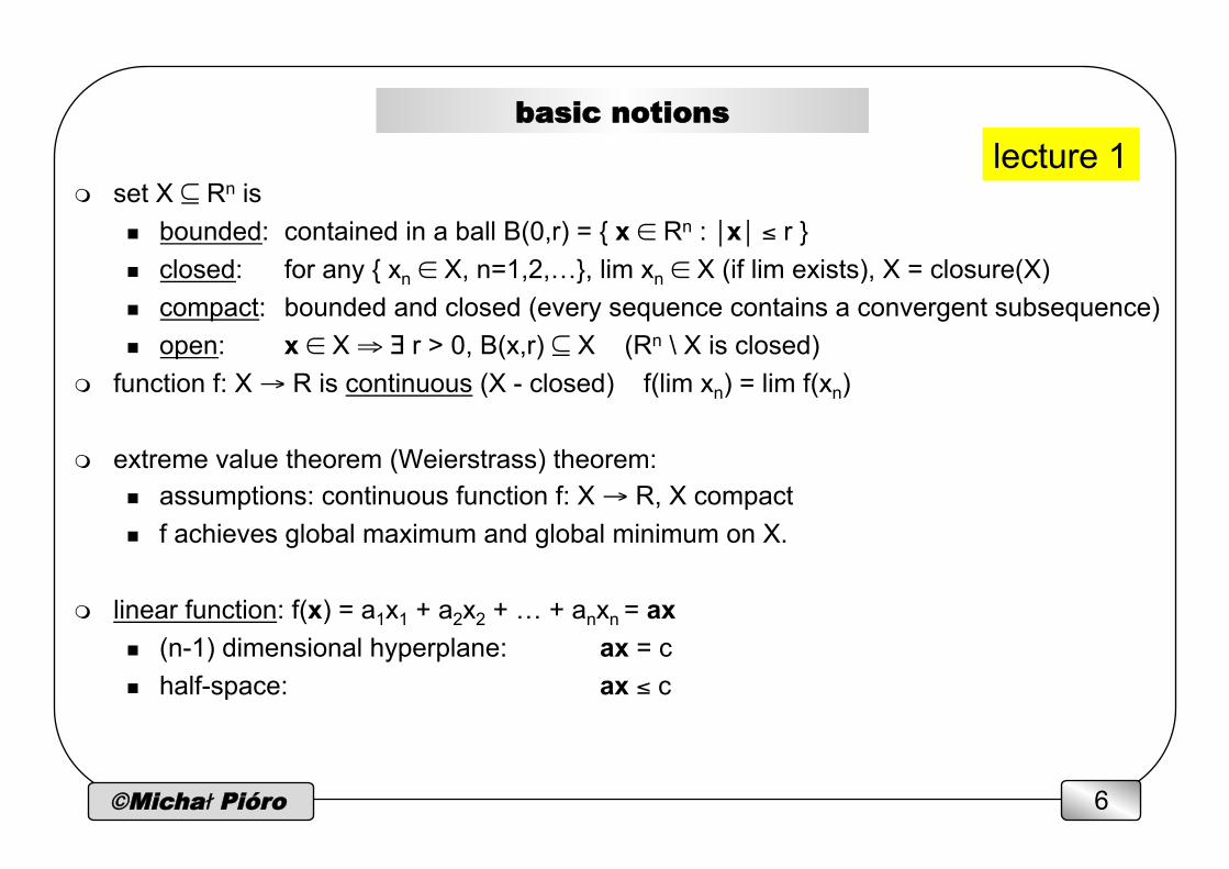
m set X ⊆ Rn is n bounded: contained in a ball B(0,r) = { x ∈ Rn : ⎪x⎪ ≤ r } n closed: for any { xn ∈ X, n=1,2,…}, lim xn ∈ X (if lim exists), X = closure(X) n compact: bounded and closed (every sequence contains a convergent subsequence) n open: x ∈ X ⇒ ∃ r > 0, B(x,r) ⊆ X (Rn \ X is closed)
m function f: X → R is continuous (X - closed) f(lim xn) = lim f(xn)
m extreme value theorem (Weierstrass) theorem: n assumptions: continuous function f: X → R, X compact n f achieves global maximum and global minimum on X.
m linear function: f(x) = a1x1 + a2x2 + … + anxn = ax n (n-1) dimensional hyperplane: ax = c n half-space: ax ≤ c
lecture 1
©Michał Pióro 7
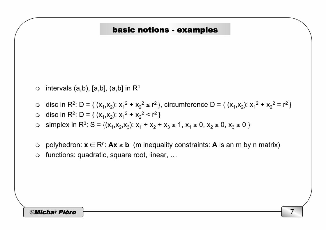
basic notions - examples
m intervals (a,b), [a,b], (a,b] in R1
m disc in R2: D = { (x1,x2): x12 + x2
2 ≤ r2 }, circumference D = { (x1,x2): x12 + x2
2 = r2 } m disc in R2: D = { (x1,x2): x1
2 + x22 < r2 }
m simplex in R3: S = {(x1,x2,x3): x1 + x2 + x3 ≤ 1, x1 ≥ 0, x2 ≥ 0, x3 ≥ 0 } m polyhedron: x ∈ Rn: Ax ≤ b (m inequality constraints: A is an m by n matrix) m functions: quadratic, square root, linear, …
©Michał Pióro 8
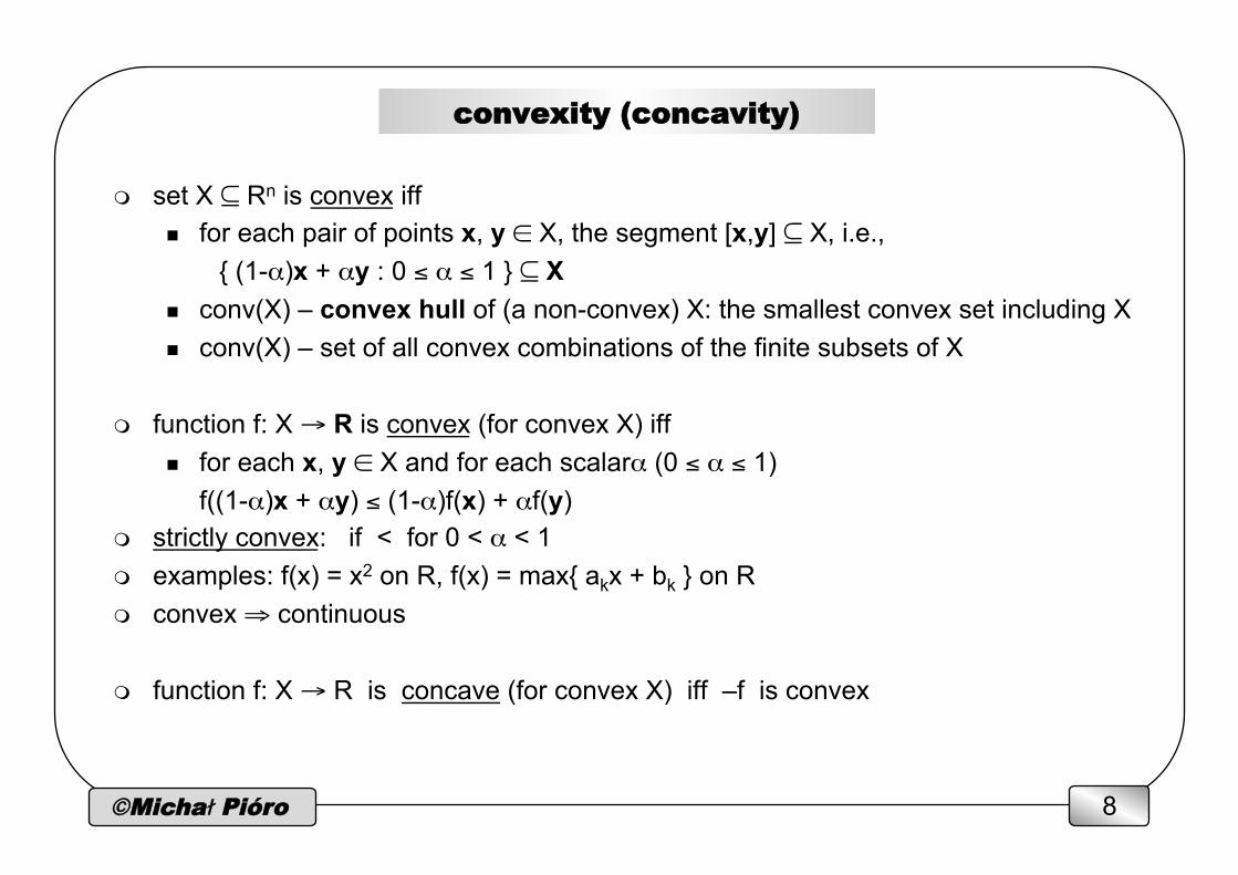
convexity (concavity)
m set X ⊆ Rn is convex iff n for each pair of points x, y ∈ X, the segment [x,y] ⊆ X, i.e.,
{ (1-α)x + αy : 0 ≤ α ≤ 1 } ⊆ X n conv(X) – convex hull of (a non-convex) X: the smallest convex set including X n conv(X) – set of all convex combinations of the finite subsets of X
m function f: X → R is convex (for convex X) iff n for each x, y ∈ X and for each scalarα (0 ≤ α ≤ 1)
f((1-α)x + αy) ≤ (1-α)f(x) + αf(y) m strictly convex: if < for 0 < α < 1 m examples: f(x) = x2 on R, f(x) = max{ akx + bk } on R m convex ⇒ continuous
m function f: X → R is concave (for convex X) iff –f is convex
©Michał Pióro 9
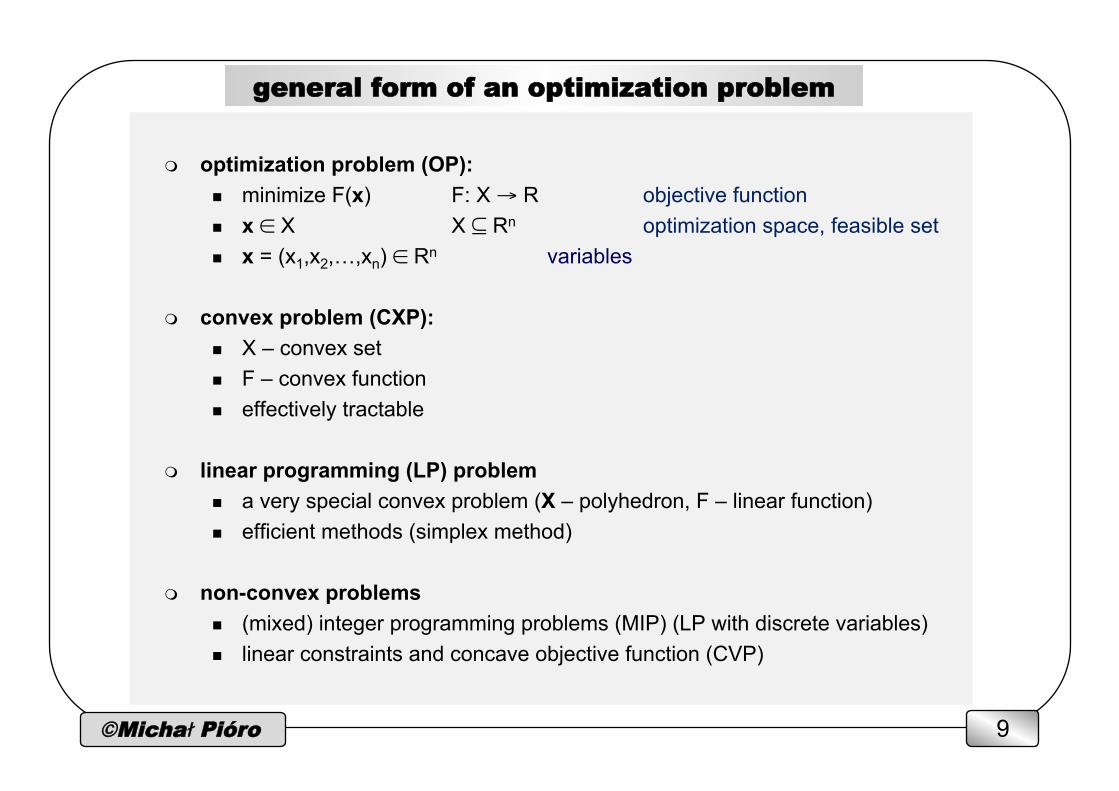
general form of an optimization problem
m optimization problem (OP): n minimize F(x) F: X → R objective function n x ∈ X X ⊆ Rn optimization space, feasible set n x = (x1,x2,…,xn) ∈ Rn variables
m convex problem (CXP): n X – convex set n F – convex function n effectively tractable
m linear programming (LP) problem n a very special convex problem (X – polyhedron, F – linear function) n efficient methods (simplex method)
m non-convex problems n (mixed) integer programming problems (MIP) (LP with discrete variables) n linear constraints and concave objective function (CVP)
©Michał Pióro 10
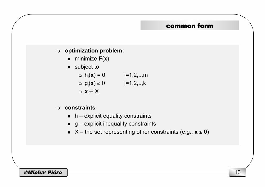
common form
m optimization problem: n minimize F(x) n subject to
❏ hi(x) = 0 i=1,2,..,m ❏ gj(x) ≤ 0 j=1,2,..,k ❏ x ∈ X
m constraints n h – explicit equality constraints n g – explicit inequality constraints n X – the set representing other constraints (e.g., x ≥ 0)

©Michał Pióro 11
relaxation - intuition
m Optimization problem (P): n minimize F(x) n x ∈ Y
m Relaxation of (P) - problem (R): n minimize G(x) n x ∈ X such that n Y ⊆ X n G(x) ≤ F(x) for all x ∈ Y
m Property (obvious): n Gopt = G(xopt(R)) ≤ F(xopt(P)) = Fopt, i.e., the optimal solution of (R) is a lower bound for (P)
m Example n linear relaxation of integer programming problem: max cx over Ax ≤ b, x - integer
©Michał Pióro 12
Dual theory
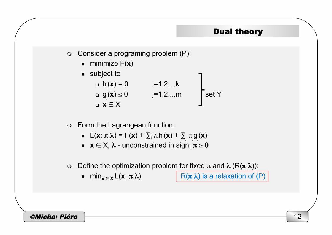
m Consider a programing problem (P): n minimize F(x) n subject to
❏ hi(x) = 0 i=1,2,..,k ❏ gj(x) ≤ 0 j=1,2,..,m set Y ❏ x ∈ X
m Form the Lagrangean function: n L(x; π,λ) = F(x) + ∑i λihi(x) + ∑j πjgj(x) n x ∈ X, λ - unconstrained in sign, π ≥ 0
m Define the optimization problem for fixed π and λ (R(π,λ)): n minx ∈ X L(x; π,λ) R(π,λ) is a relaxation of (P)

©Michał Pióro 13
why the dual is a relaxation?
m Problem (R(π,λ)): n minimize G(x) = F(x) + ∑i λihi(x) + ∑j πjgj(x) (π, λ are given!) n subject to
❏ x ∈ X n W(π,λ) = Gopt
m hence n Y ⊆ X (trivially) n G(x) ≤ F(x) for all x ∈ Y (because πj ≥ 0, and for all x ∈ Y, gj(x) ≤ 0 and hi(x) = 0)
m and n W(π,λ) ≤ F(xopt(P)) for all (π,λ) ∈ Dom(W)
©Michał Pióro 14
dual problem
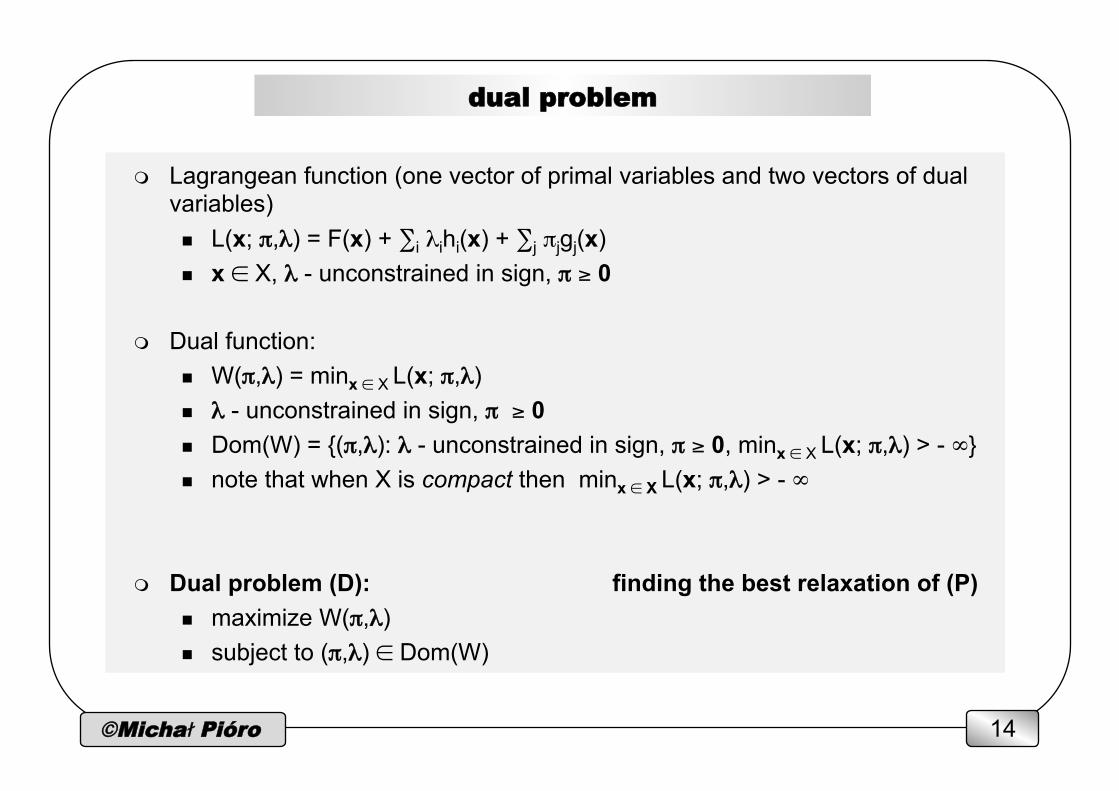
m Lagrangean function (one vector of primal variables and two vectors of dual variables) n L(x; π,λ) = F(x) + ∑i λihi(x) + ∑j πjgj(x) n x ∈ X, λ - unconstrained in sign, π ≥ 0
m Dual function: n W(π,λ) = minx ∈ X L(x; π,λ) n λ - unconstrained in sign, π ≥ 0 n Dom(W) = {(π,λ): λ - unconstrained in sign, π ≥ 0, minx ∈ X L(x; π,λ) > - ∞} n note that when X is compact then minx ∈ X L(x; π,λ) > - ∞
m Dual problem (D): finding the best relaxation of (P) n maximize W(π,λ) n subject to (π,λ) ∈ Dom(W)
©Michał Pióro 15
duality – basic properties for general problems
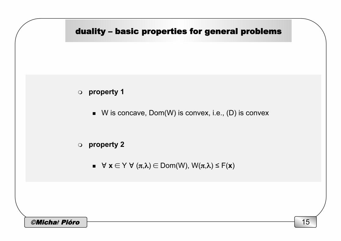
m property 1
n W is concave, Dom(W) is convex, i.e., (D) is convex
m property 2
n ∀ x ∈ Y ∀ (π,λ) ∈ Dom(W), W(π,λ) ≤ F(x)
©Michał Pióro 16
convex problems
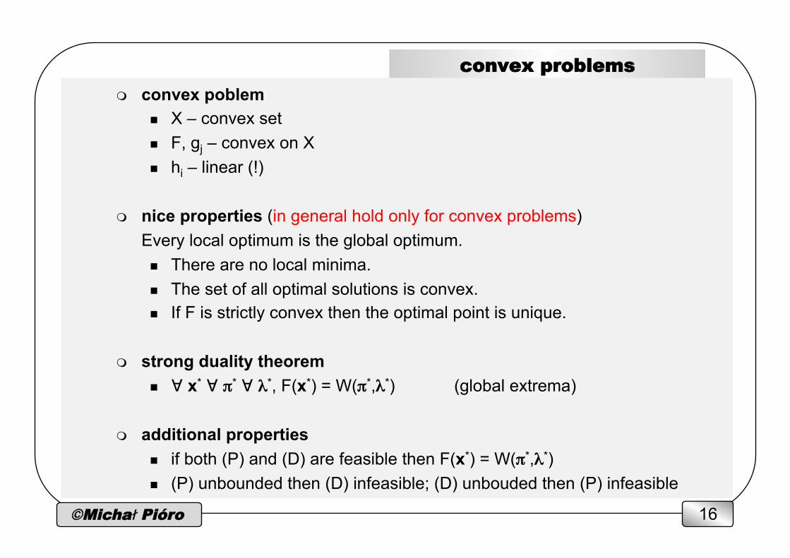
m convex poblem n X – convex set n F, gj – convex on X n hi – linear (!)
m nice properties (in general hold only for convex problems) Every local optimum is the global optimum.
n There are no local minima. n The set of all optimal solutions is convex. n If F is strictly convex then the optimal point is unique.
m strong duality theorem n ∀ x* ∀ π* ∀ λ*, F(x*) = W(π*,λ*) (global extrema)
m additional properties n if both (P) and (D) are feasible then F(x*) = W(π*,λ*) n (P) unbounded then (D) infeasible; (D) unbouded then (P) infeasible
©Michał Pióro 17
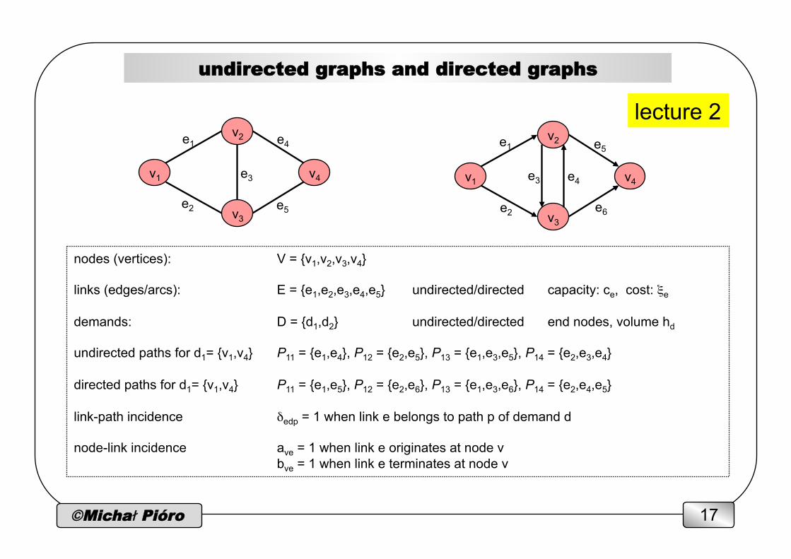
undirected graphs and directed graphs
nodes (vertices): V = {v1,v2,v3,v4} links (edges/arcs): E = {e1,e2,e3,e4,e5} undirected/directed capacity: ce, cost: ξe demands: D = {d1,d2} undirected/directed end nodes, volume hd undirected paths for d1= {v1,v4} P11 = {e1,e4}, P12 = {e2,e5}, P13 = {e1,e3,e5}, P14 = {e2,e3,e4} directed paths for d1= {v1,v4} P11 = {e1,e5}, P12 = {e2,e6}, P13 = {e1,e3,e6}, P14 = {e2,e4,e5} link-path incidence δedp = 1 when link e belongs to path p of demand d node-link incidence ave = 1 when link e originates at node v
bve = 1 when link e terminates at node v
v2
v1 v4
v3
v2
v1 v4
v3
e1
e2 e5
e4
e3
e1
e2
e3 e4
e5
e6
lecture 2
©Michał Pióro 18
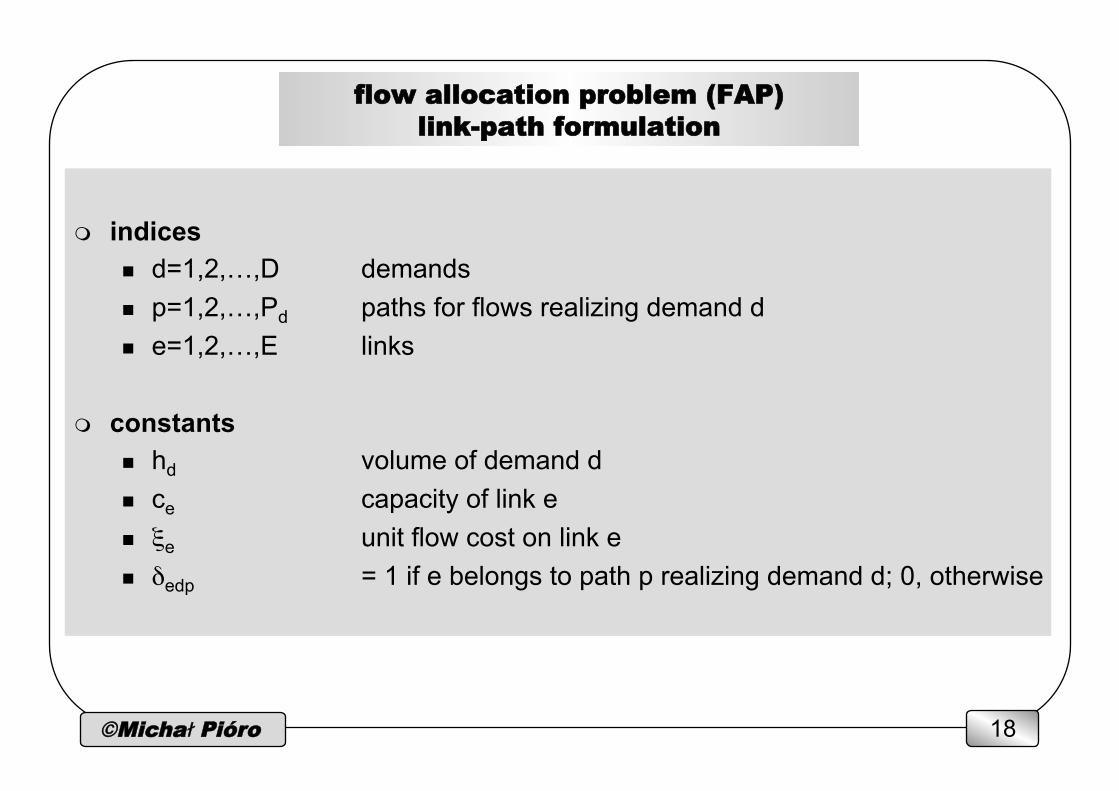
flow allocation problem (FAP) link-path formulation
m indices n d=1,2,…,D demands
n p=1,2,…,Pd paths for flows realizing demand d n e=1,2,…,E links
m constants n hd volume of demand d n ce capacity of link e n ξe unit flow cost on link e n δedp = 1 if e belongs to path p realizing demand d; 0, otherwise
©Michał Pióro 19
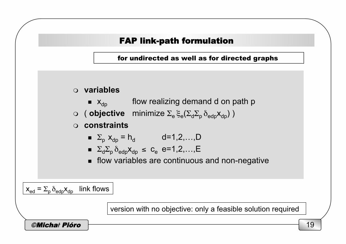
FAP link-path formulation
m variables n xdp flow realizing demand d on path p
m ( objective minimize Σe ξe(ΣdΣp δedpxdp) ) m constraints
n Σp xdp = hd d=1,2,…,D n ΣdΣp δedpxdp ≤ ce e=1,2,…,E n flow variables are continuous and non-negative
version with no objective: only a feasible solution required
for undirected as well as for directed graphs
xed = Σp δedpxdp link flows
©Michał Pióro 20
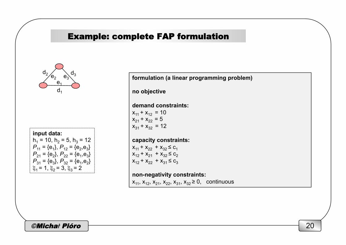
Example: complete FAP formulation
input data: h1 = 10, h2 = 5, h3 = 12 P11 = {e1}, P12 = {e2,e3} P21 = {e2}, P22 = {e1,e3} P31 = {e3}, P32 = {e1,e2} ξ1 = 1, ξ2 = 3, ξ3 = 2
formulation (a linear programming problem) no objective demand constraints: x11 + x12 = 10 x21 + x22 = 5 x31 + x32 = 12 capacity constraints: x11 + x22 + x32 ≤ c1 x12 + x21 + x32 ≤ c2 x12 + x22 + x31 ≤ c3 non-negativity constraints: x11, x12, x21, x22, x31, x32 ≥ 0, continuous
d1
e3 e2 e1
d3 d2
©Michał Pióro 21
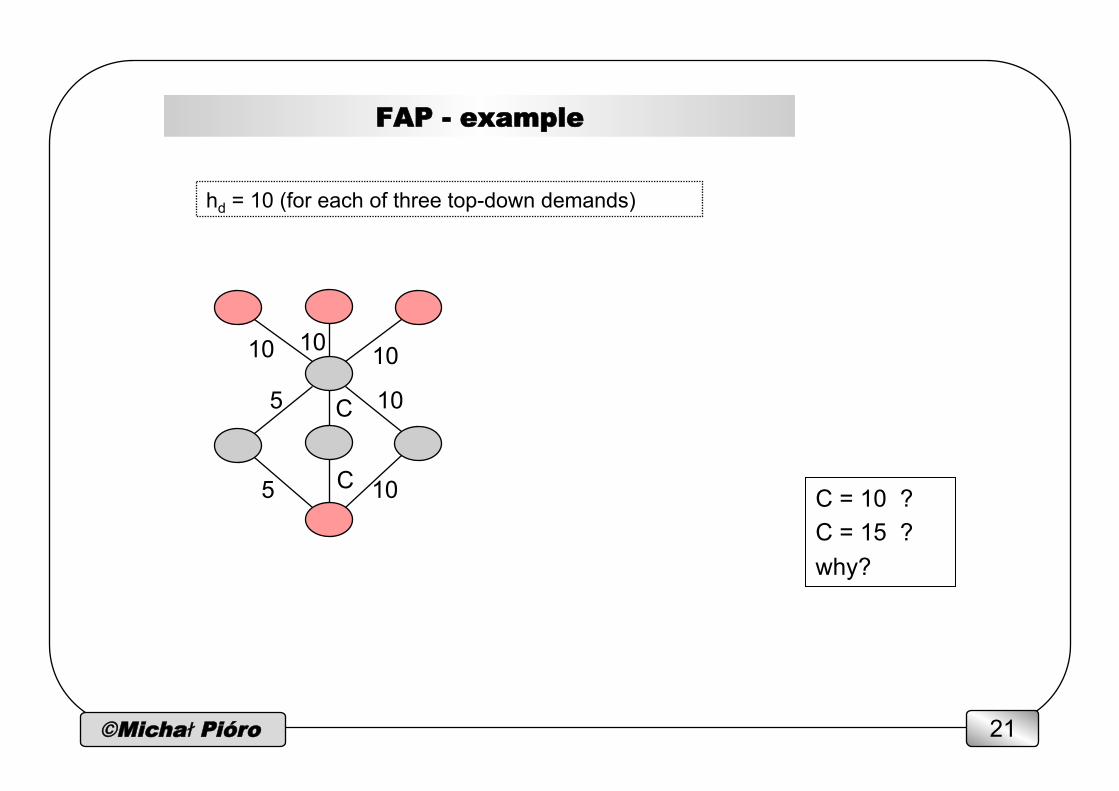
FAP - example
hd = 10 (for each of three top-down demands)
10
5
5
10
10
10 10
C
C C = 10 ? C = 15 ? why?
©Michał Pióro 22
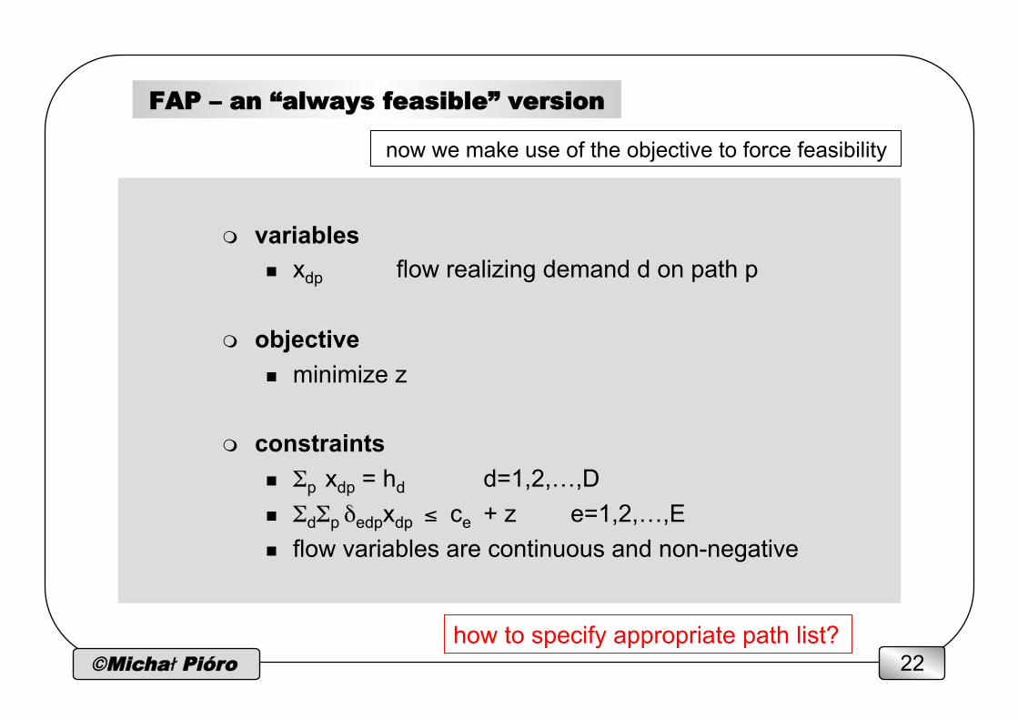
FAP – an “always feasible” version
m variables
n xdp flow realizing demand d on path p
m objective n minimize z
m constraints n Σp xdp = hd d=1,2,…,D n ΣdΣp δedpxdp ≤ ce + z e=1,2,…,E n flow variables are continuous and non-negative
now we make use of the objective to force feasibility
how to specify appropriate path list?

©Michał Pióro 23
example of the difficulty
the number of paths in the graph grows exponentially so we simply cannot put them all on the path lists!
5 by 5 Manhattan network: 840 shortest-hop paths between two
opposite corners
h = 1 + ε
c = 1 + ε c = 1 + ε
c = 1 + ε c = 1 + ε all 10 demands but one with h = 1 all 10 links but four with capacity 1 how should we know that the thick path must be used to get the optimal solution?

©Michał Pióro 24
The number of shortest paths (each shortest path has 2(n-1) links) from s to t is equal to
(2n-2) over (n-1) in the sense of the Newton symbol. In the above example it is 4 over 2, i.e., 6. In general, when we have n x m nodes (n in the horizontal direction, and m in vertical), the formula reads
(n+m-2) over (m-1) which is equal to (m+n-2) over (n-1).
n = 3
s
t
number of paths in Manhattan
©Michał Pióro 25
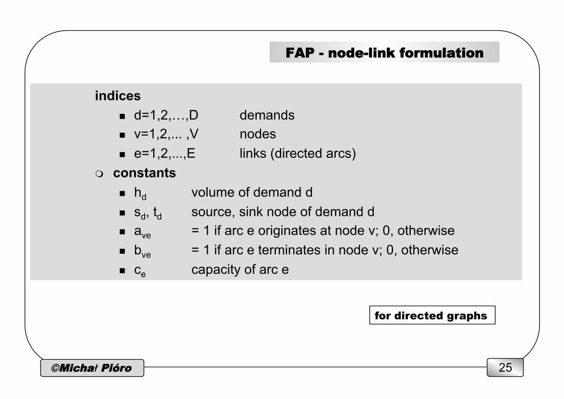
FAP - node-link formulation
indices n d=1,2,…,D demands
n v=1,2,... ,V nodes n e=1,2,...,E links (directed arcs)
m constants n hd volume of demand d n sd, td source, sink node of demand d n ave = 1 if arc e originates at node v; 0, otherwise n bve = 1 if arc e terminates in node v; 0, otherwise n ce capacity of arc e
for directed graphs
©Michał Pióro 26
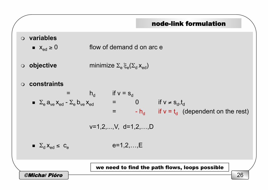
node-link formulation
m variables n xed ≥ 0 flow of demand d on arc e
m objective minimize Σe ξe(Σd xed)
m constraints = hd if v = sd
n Σe ave xed - Σe bve xed = 0 if v ≠ sd,td
= - hd if v = td (dependent on the rest)
v=1,2,...,V, d=1,2,…,D
n Σd xed ≤ ce e=1,2,…,E
we need to find the path flows, loops possible
©Michał Pióro 27
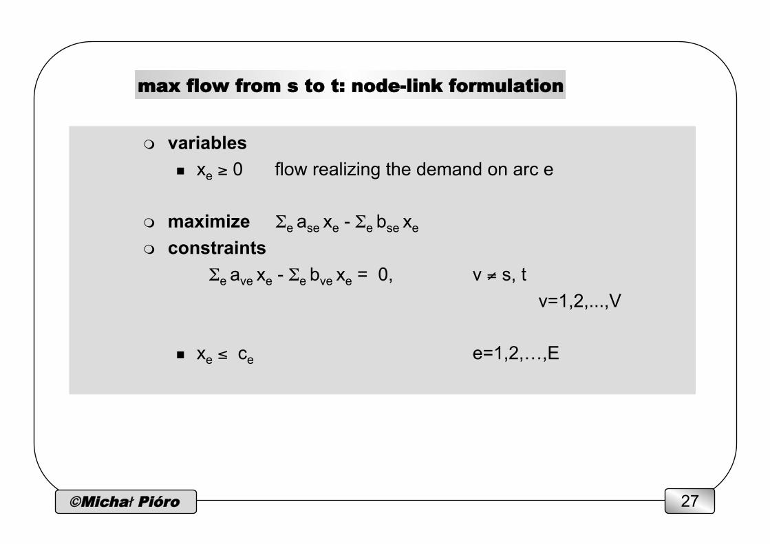
max flow from s to t: node-link formulation
m variables n xe ≥ 0 flow realizing the demand on arc e
m maximize Σe ase xe - Σe bse xe m constraints
Σe ave xe - Σe bve xe = 0, v ≠ s, t v=1,2,...,V
n xe ≤ ce e=1,2,…,E
©Michał Pióro 28
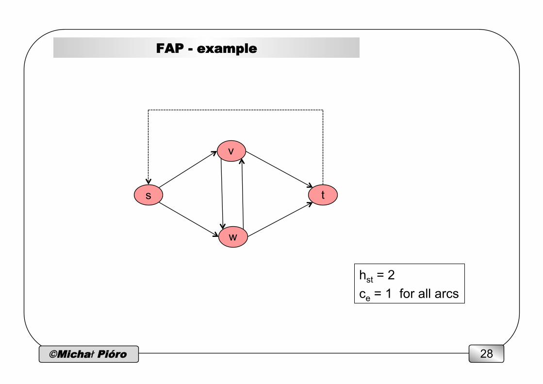
FAP - example
w
v
t s
hst = 2 ce = 1 for all arcs
©Michał Pióro 29
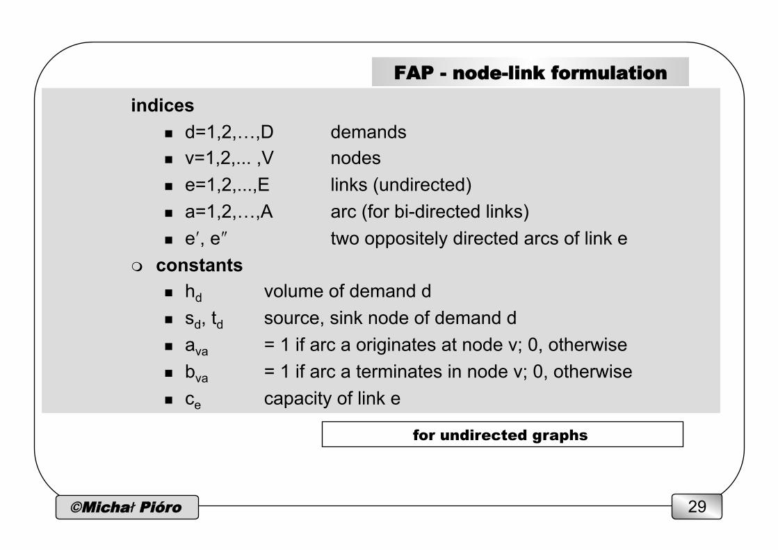
FAP - node-link formulation
indices n d=1,2,…,D demands
n v=1,2,... ,V nodes n e=1,2,...,E links (undirected) n a=1,2,…,A arc (for bi-directed links) n eʹ′, eʺ″ two oppositely directed arcs of link e
m constants n hd volume of demand d n sd, td source, sink node of demand d n ava = 1 if arc a originates at node v; 0, otherwise n bva = 1 if arc a terminates in node v; 0, otherwise n ce capacity of link e
for undirected graphs
©Michał Pióro 30
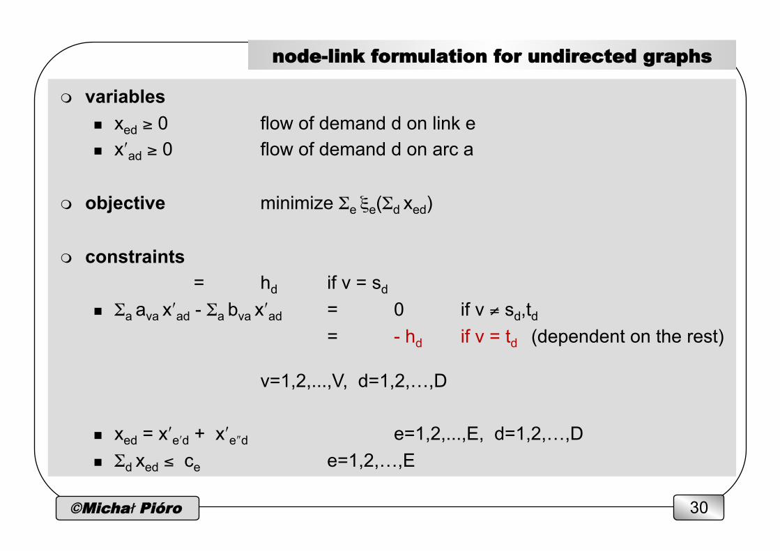
node-link formulation for undirected graphs
m variables n xed ≥ 0 flow of demand d on link e n xʹ′ad ≥ 0 flow of demand d on arc a
m objective minimize Σe ξe(Σd xed)
m constraints = hd if v = sd
n Σa ava xʹ′ad - Σa bva xʹ′ad = 0 if v ≠ sd,td
= - hd if v = td (dependent on the rest)
v=1,2,...,V, d=1,2,…,D
n xed = xʹ′eʹ′d + xʹ′eʺ″d e=1,2,...,E, d=1,2,…,Dn Σd xed ≤ ce e=1,2,…,E
©Michał Pióro 31
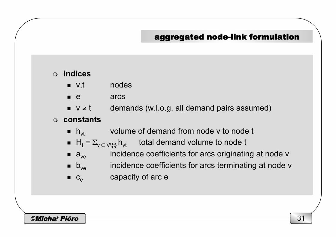
aggregated node-link formulation
m indices
n v,t nodes n e arcs n v ≠ t demands (w.l.o.g. all demand pairs assumed)
m constants n hvt volume of demand from node v to node t n Ht = Σv ∈ V\{t} hvt total demand volume to node t n ave incidence coefficients for arcs originating at node v n bve incidence coefficients for arcs terminating at node v n ce capacity of arc e
©Michał Pióro 32
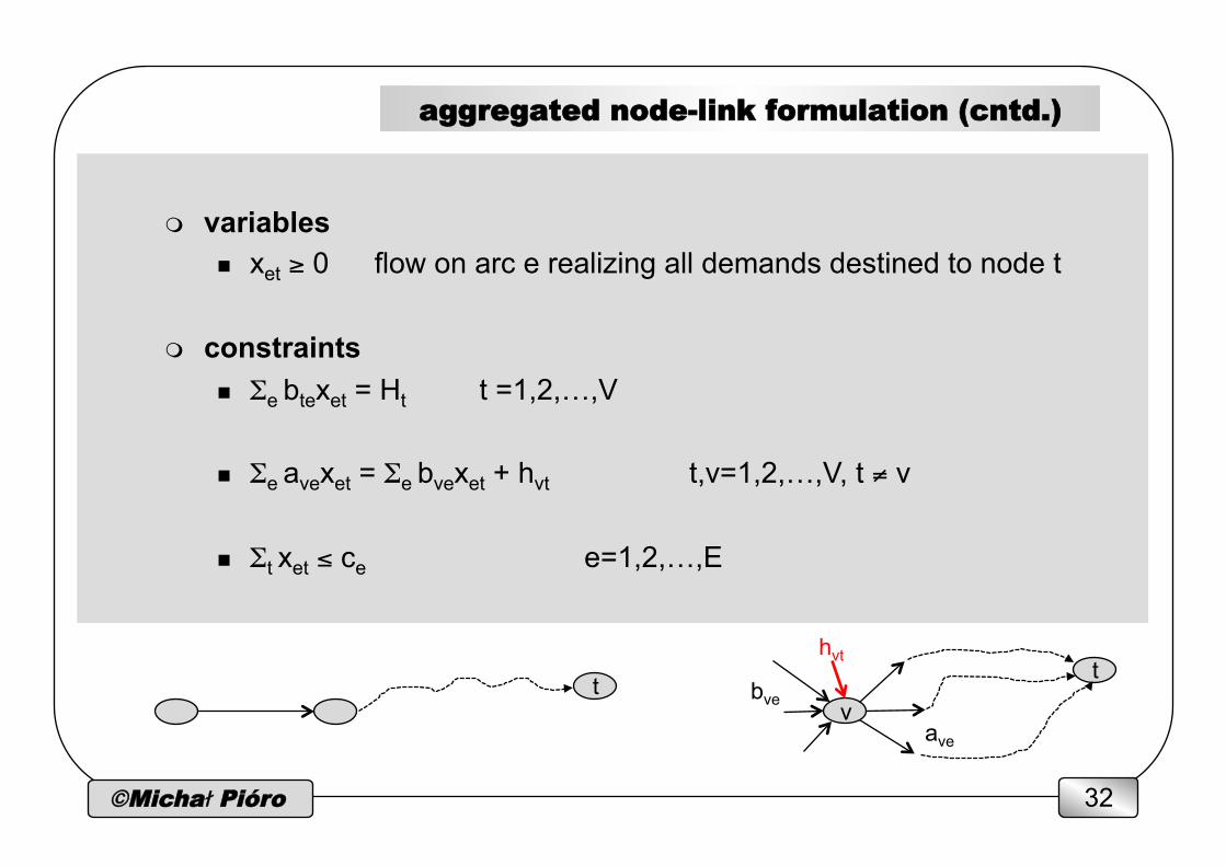
aggregated node-link formulation (cntd.)
m variables n xet ≥ 0 flow on arc e realizing all demands destined to node t
m constraints n Σe btexet = Ht t =1,2,…,V
n Σe avexet = Σe bvexet + hvt t,v=1,2,…,V, t ≠ v
n Σt xet ≤ ce e=1,2,…,E
t v
bve
hvt t
ave
©Michał Pióro 33
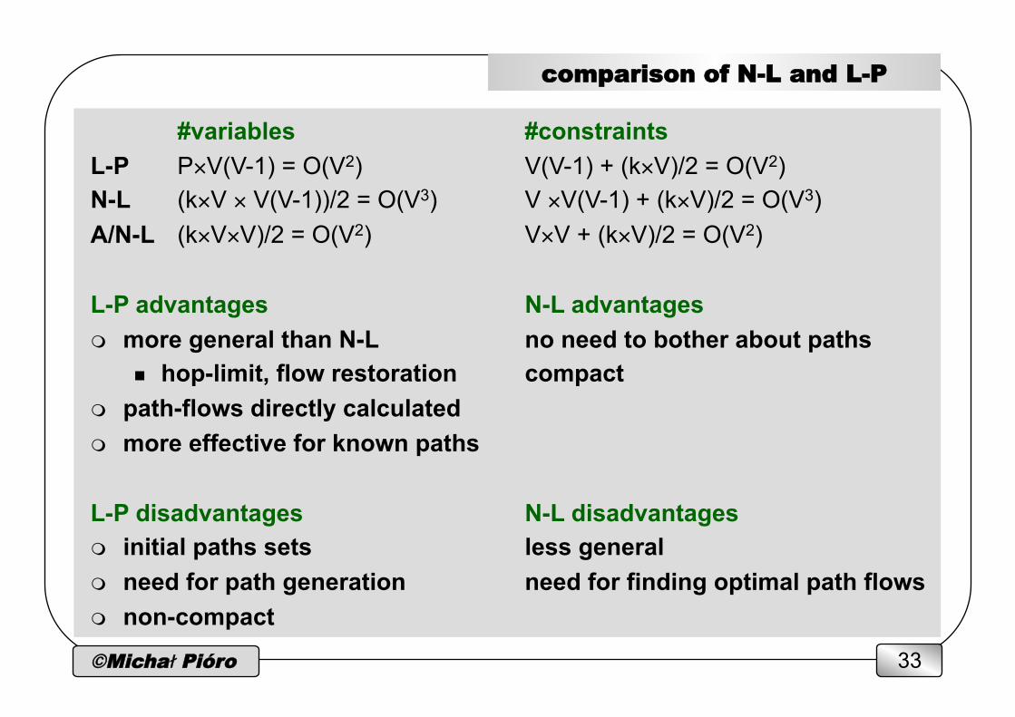
comparison of N-L and L-P
#variables #constraints L-P P×V(V-1) = O(V2) V(V-1) + (k×V)/2 = O(V2) N-L (k×V × V(V-1))/2 = O(V3) V ×V(V-1) + (k×V)/2 = O(V3) A/N-L (k×V×V)/2 = O(V2) V×V + (k×V)/2 = O(V2) L-P advantages N-L advantages m more general than N-L no need to bother about paths
n hop-limit, flow restoration compact m path-flows directly calculated m more effective for known paths L-P disadvantages N-L disadvantages m initial paths sets less general m need for path generation need for finding optimal path flows m non-compact
©Michał Pióro 34
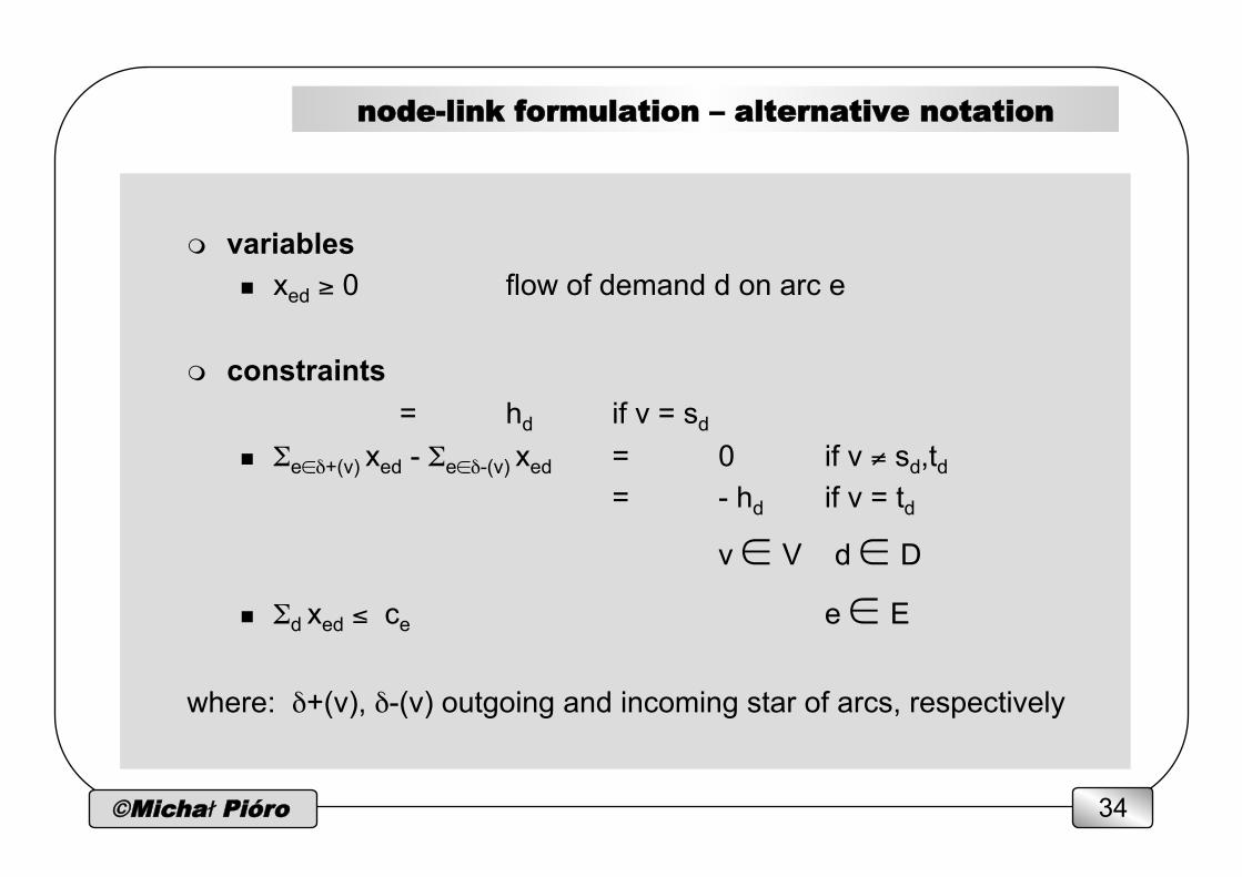
node-link formulation – alternative notation
m variables n xed ≥ 0 flow of demand d on arc e
m constraints = hd if v = sd
n Σe∈δ+(v) xed - Σe∈δ-(v) xed = 0 if v ≠ sd,td
= - hd if v = td
v ∈ V d ∈ Dn Σd xed ≤ ce e ∈ E
where: δ+(v), δ-(v) outgoing and incoming star of arcs, respectively
©Michał Pióro 35
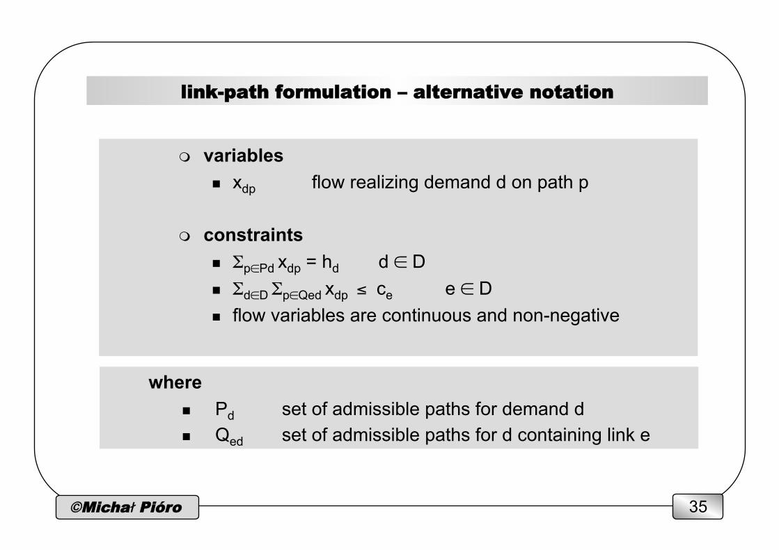
link-path formulation – alternative notation
m variables n xdp flow realizing demand d on path p
m constraints n Σp∈Pd xdp = hd d ∈ D n Σd∈D Σp∈Qed xdp ≤ ce e ∈ D n flow variables are continuous and non-negative
where n Pd set of admissible paths for demand d n Qed set of admissible paths for d containing link e
©Michał Pióro 36
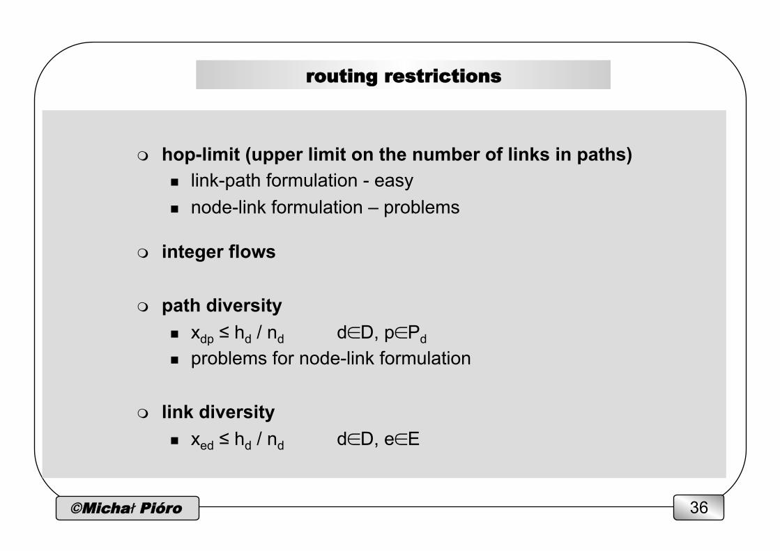
routing restrictions
m hop-limit (upper limit on the number of links in paths) n link-path formulation - easy n node-link formulation – problems
m integer flows
m path diversity n xdp ≤ hd / nd d∈D, p∈Pd
n problems for node-link formulation
m link diversity n xed ≤ hd / nd d∈D, e∈E
©Michał Pióro 37
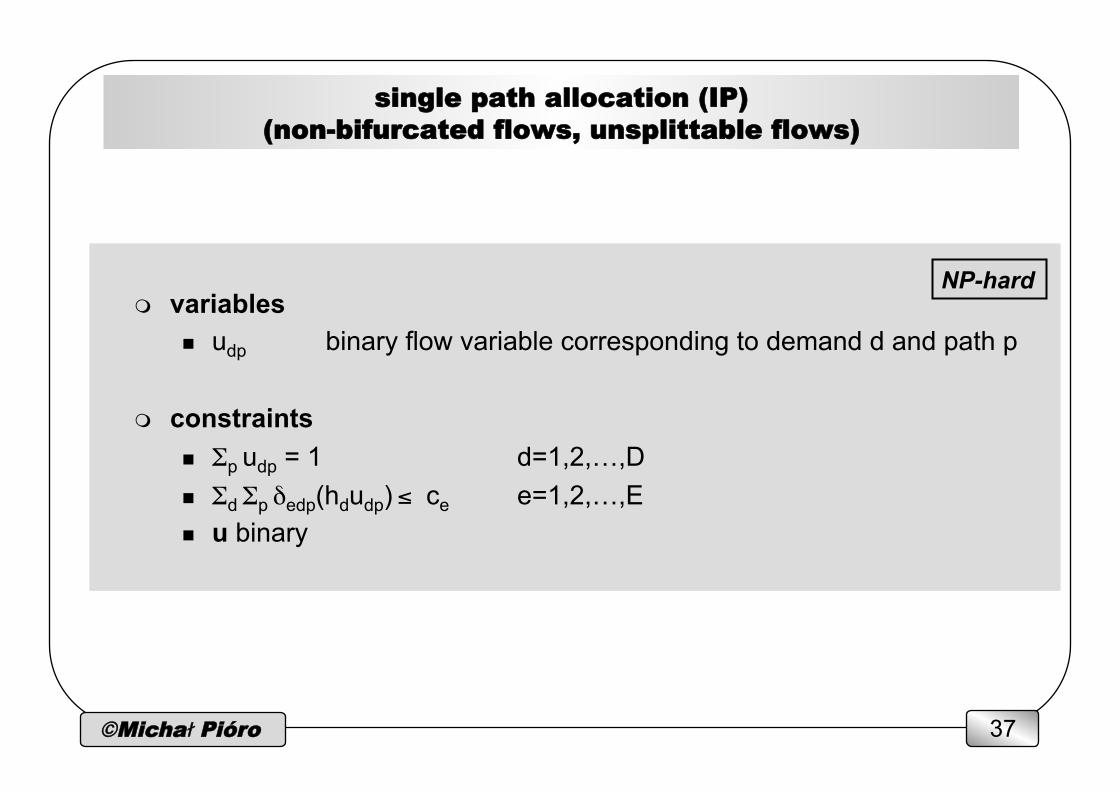
single path allocation (IP) (non-bifurcated flows, unsplittable flows)
m variables n udp binary flow variable corresponding to demand d and path p
m constraints n Σp udp = 1 d=1,2,…,D n Σd Σp δedp(hdudp) ≤ ce e=1,2,…,E n u binary
NP-hard
©Michał Pióro 38
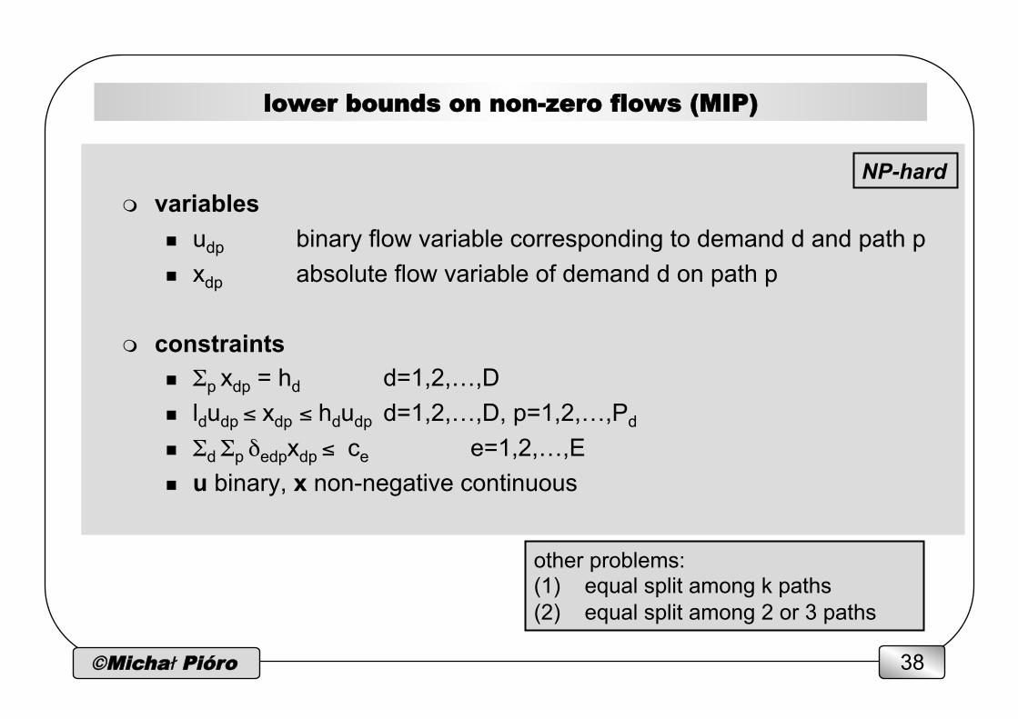
lower bounds on non-zero flows (MIP)
m variables n udp binary flow variable corresponding to demand d and path p n xdp absolute flow variable of demand d on path p
m constraints n Σp xdp = hd d=1,2,…,D n ldudp ≤ xdp ≤ hdudp d=1,2,…,D, p=1,2,…,Pd n Σd Σp δedpxdp ≤ ce e=1,2,…,E n u binary, x non-negative continuous
other problems: (1) equal split among k paths (2) equal split among 2 or 3 paths
NP-hard
©Michał Pióro 39
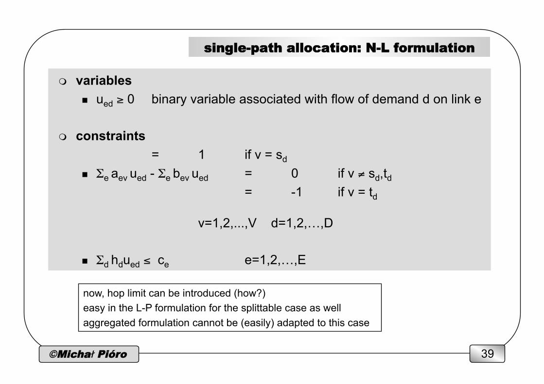
single-path allocation: N-L formulation
m variables n ued ≥ 0 binary variable associated with flow of demand d on link e
m constraints = 1 if v = sd
n Σe aev ued - Σe bev ued = 0 if v ≠ sd,td
= -1 if v = td
v=1,2,...,V d=1,2,…,D
n Σd hdued ≤ ce e=1,2,…,E
now, hop limit can be introduced (how?) easy in the L-P formulation for the splittable case as well aggregated formulation cannot be (easily) adapted to this case
©Michał Pióro 40
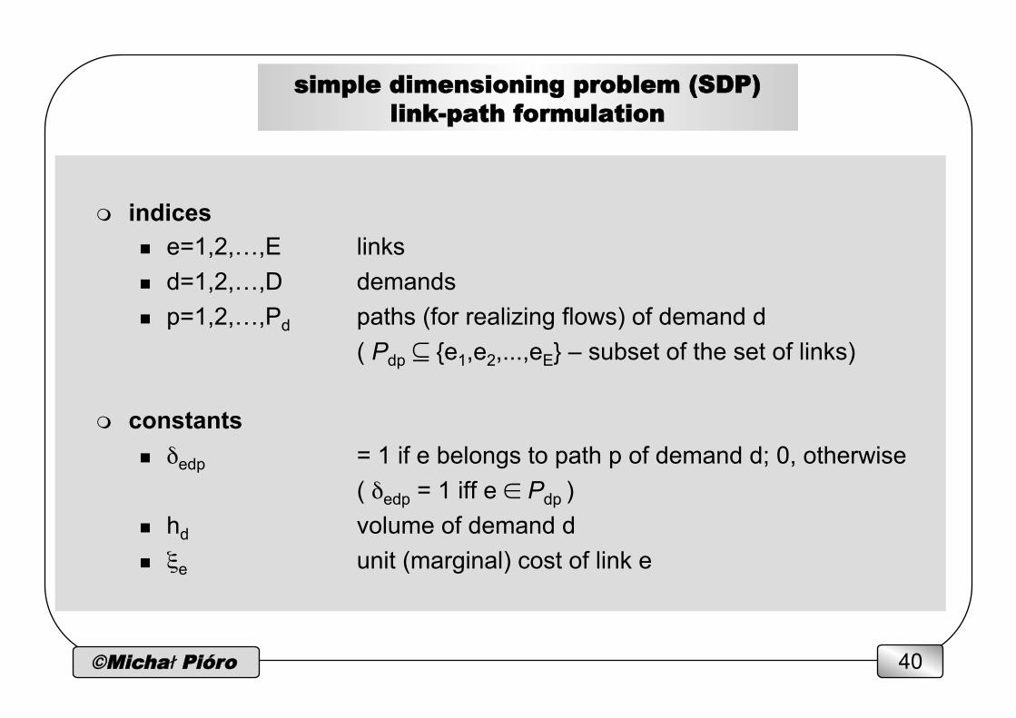
simple dimensioning problem (SDP) link-path formulation
m indices n e=1,2,…,E links n d=1,2,…,D demands
n p=1,2,…,Pd paths (for realizing flows) of demand d ( Pdp ⊆ {e1,e2,...,eE} – subset of the set of links)
m constants n δedp = 1 if e belongs to path p of demand d; 0, otherwise
( δedp = 1 iff e ∈ Pdp ) n hd volume of demand d n ξe unit (marginal) cost of link e

©Michał Pióro 41
SDP formulation
m variables n xdp continuous flow realizing demand d on path p n ye continuous capacity of link e
m objective minimize F(y) = Σe ξeye
m constraints
n Σp xdp = hd d=1,2,…,D n Σd Σp δedpxdp = ye e=1,2,…,E n variables x, y are continuous and non-negative
how to solve this problem?

©Michał Pióro 42
SDP – complete example formulation
input data: h1 = 10, h2 = 5, h3 = 12 P11 = {e1}, P12 = {e2,e3} P21 = {e2}, P22 = {e1,e3} P31 = {e3}, P32 = {e1,e2} ξ1 = 1, ξ2 = 3, ξ3 = 2
formulation (a linear programming problem) objective: minimize y1 + 3y2 + 2y3 demand constraints: x11 + x12 = 10 x21 + x22 = 5 x31 + x32 = 12 capacity constraints: x11 + x22 + x32 = y1 x12 + x21 + x32 = y2 x12 + x22 + x31 = y3 non-negativity constraints: x11, x12, x21, x22, x31, x32 ≥ 0, continuous
d1
e3 e2 e1
d3 d2

©Michał Pióro 43
SDP - example
ξe = 3 (black links) ξe =1 (red links)
allowable paths for d=4, h4 = 10 P41 = {e3,e6,e9}, P42 = {e1,e4,e9}, P43 = {e3,e6,e8,e11}, … demand constraint for d=4, h4 = 10 x41 + x42 + x43 + … = 10 capacity constraints (on the blackboard)
d1
e11 e9
e10
e8
e7
e6
e5
e4
e3
e2
e1
d5
d3
d2
d4

©Michał Pióro 44
solving SDP
m minimize F(y) = Σe ξeye n Σp xdp = hd d=1,2,…,D n Σd Σp δedpxdp = ye e=1,2,…,E
m minimize F = Σe ξe (Σd Σp δedpxdp) = Σd Σp (Σe ξeδedp)xdp n Σp xdp = hd d=1,2,…,D
m for each d=1,2,…,D separately minimize F = Σp (Σe ξeδedp)xdp
n Σp xdp = hd d=1,2,…,D

©Michał Pióro 45
solution – shortest path allocation rule (SPAR)
m for a fixed d minimize F = Σp (Σe ξeδedp)xdp = Σp κdpxdp = αdhd
n Σp xdp = hd d=1,2,…,D
m solution: F = Σd αdhd where
κdp - cost of path p of demand d αd – cost of the cheapest (shortest with respect to ξe) path of demand d let p(d) be such a path (Σe∈Pdp(d) ξe = αd)
m solution: put the whole demand on the shortest path: n x*dp(d) := hd ; x*dp := 0, p ≠ p(d) n we may also split hd arbitrarily over the shortest paths for d
©Michał Pióro 46
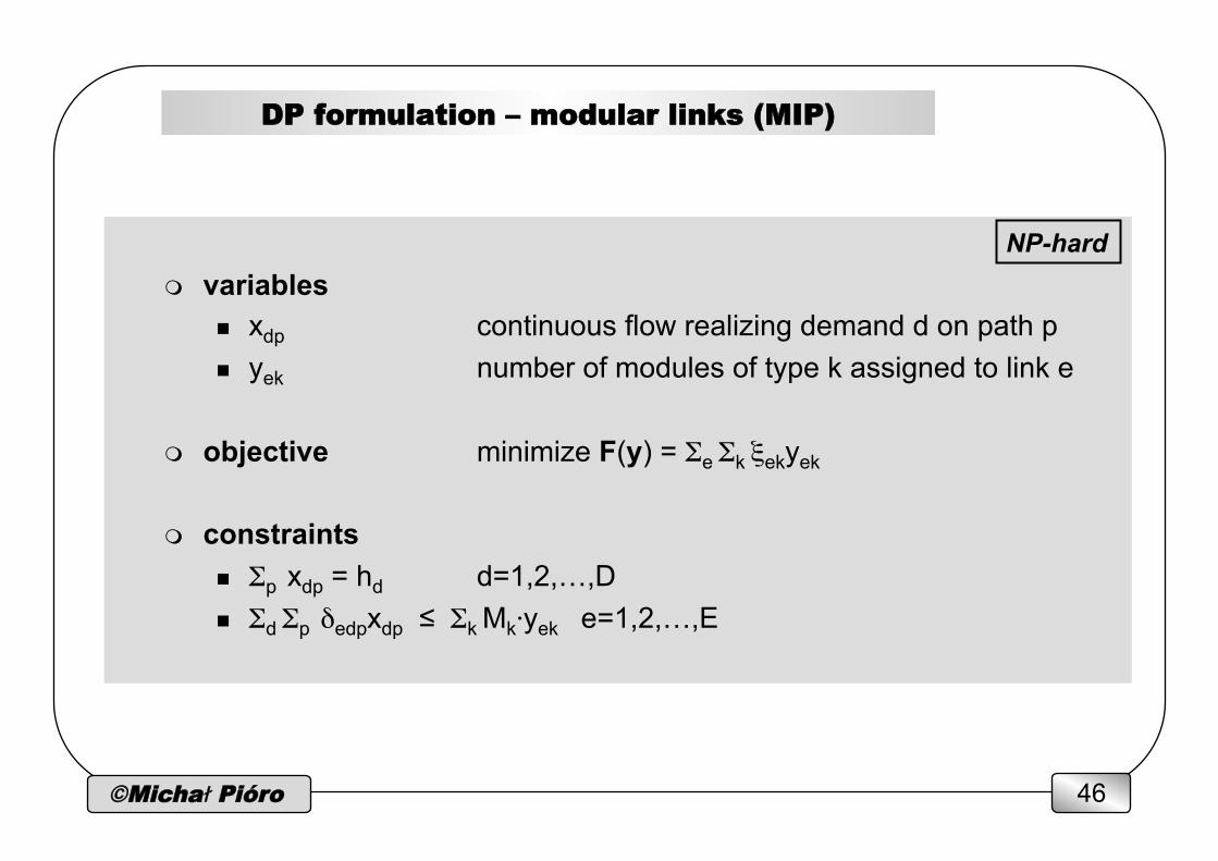
DP formulation – modular links (MIP)
m variables n xdp continuous flow realizing demand d on path p n yek number of modules of type k assigned to link e
m objective minimize F(y) = Σe Σk ξekyek
m constraints
n Σp xdp = hd d=1,2,…,D n Σd Σp δedpxdp ≤ Σk Mk⋅yek e=1,2,…,E
NP-hard
©Michał Pióro 47
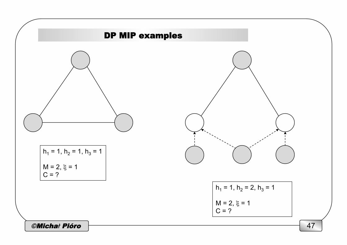
DP MIP examples
h1 = 1, h2 = 1, h3 = 1 M = 2, ξ = 1 C = ?
h1 = 1, h2 = 2, h3 = 1 M = 2, ξ = 1 C = ?
©Michał Pióro 48
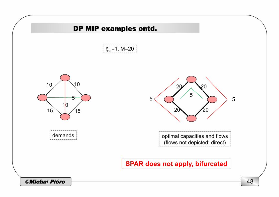
DP MIP examples cntd.
ξe =1, M=20
SPAR does not apply, bifurcated
10
5
15 10
10
15
demands optimal capacities and flows (flows not depicted: direct)
20
20
20
20
5 5 5
©Michał Pióro 49
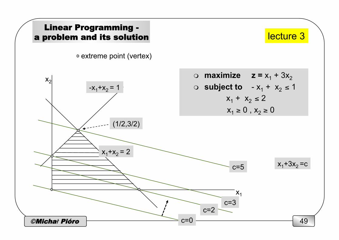
Linear Programming - a problem and its solution
m maximize z = x1 + 3x2 m subject to - x1 + x2 ≤ 1
x1 + x2 ≤ 2 x1 ≥ 0 , x2 ≥ 0
x2
x1
-x1+x2 = 1
x1+3x2 =c c=5
c=3
c=0
(1/2,3/2)
extreme point (vertex)
c=2
x1+x2 = 2
lecture 3
©Michał Pióro 50
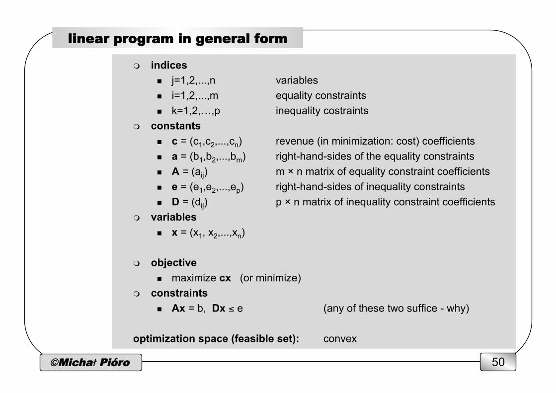
linear program in general form
m indices n j=1,2,...,n variables n i=1,2,...,m equality constraints n k=1,2,…,p inequality costraints
m constants n c = (c1,c2,...,cn) revenue (in minimization: cost) coefficients n a = (b1,b2,...,bm) right-hand-sides of the equality constraints n A = (aij) m × n matrix of equality constraint coefficients n e = (e1,e2,...,ep) right-hand-sides of inequality constraints n D = (dij) p × n matrix of inequality constraint coefficients
m variables n x = (x1, x2,...,xn)
m objective n maximize cx (or minimize)
m constraints n Ax = b, Dx ≤ e (any of these two suffice - why)
optimization space (feasible set): convex
©Michał Pióro 51
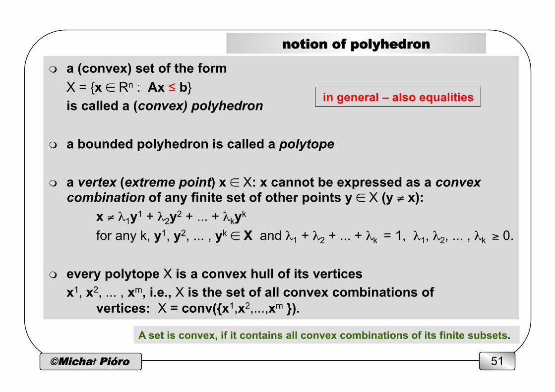
notion of polyhedron
m a (convex) set of the form X = {x ∈ Rn : Ax ≤ b} is called a (convex) polyhedron
m a bounded polyhedron is called a polytope
m a vertex (extreme point) x ∈ X: x cannot be expressed as a convex combination of any finite set of other points y ∈ X (y ≠ x): x ≠ λ1y1 + λ2y2 + ... + λkyk for any k, y1, y2, ... , yk ∈ X and λ1 + λ2 + ... + λk = 1, λ1, λ2, ... , λk ≥ 0.
m every polytope X is a convex hull of its vertices
x1, x2, ... , xm, i.e., X is the set of all convex combinations of vertices: X = conv({x1,x2,...,xm }).
in general – also equalities
A set is convex, if it contains all convex combinations of its finite subsets.
©Michał Pióro 52
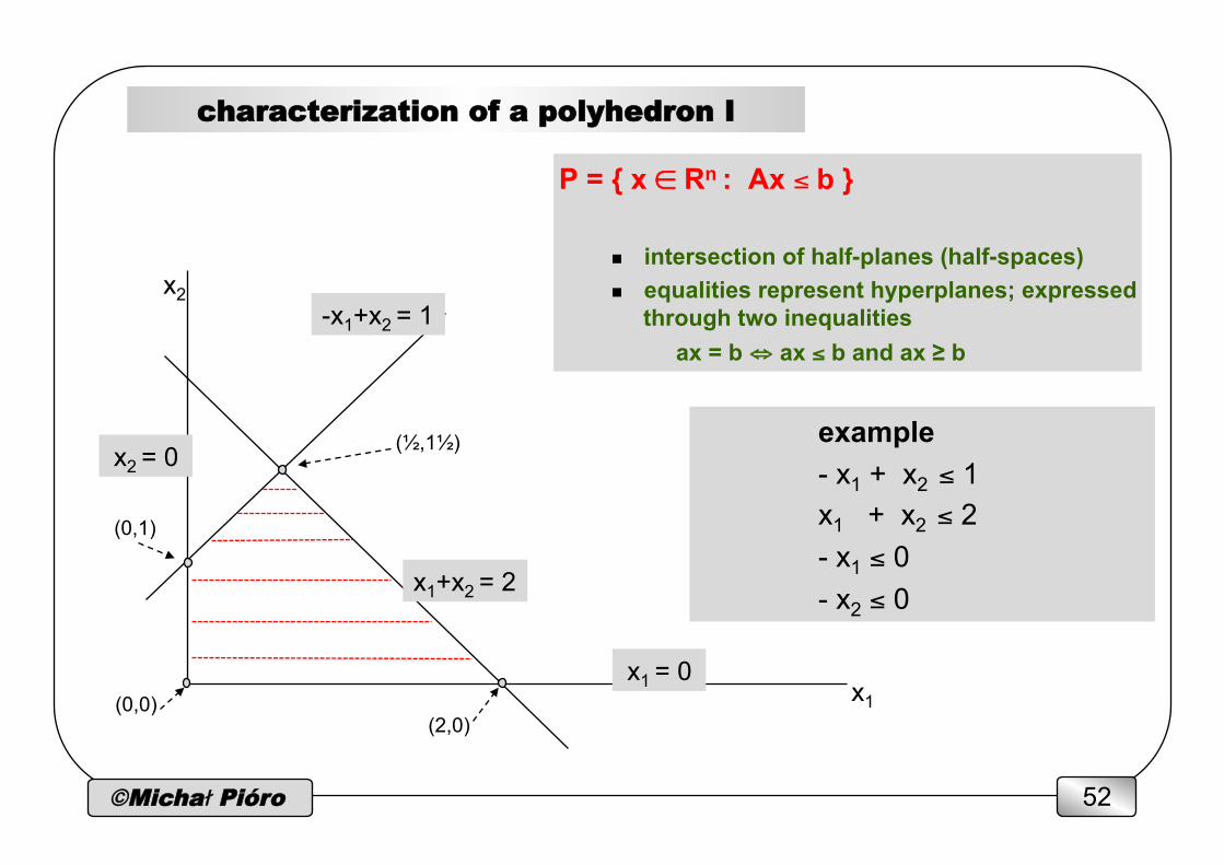
characterization of a polyhedron I
P = { x ∈ Rn : Ax ≤ b }
n intersection of half-planes (half-spaces) n equalities represent hyperplanes; expressed
through two inequalities ax = b ⇔ ax ≤ b and ax ≥ b
x2
x1
-x1+x2 = 1
x1+x2 = 2
(½,1½) example - x1 + x2 ≤ 1 x1 + x2 ≤ 2 - x1 ≤ 0 - x2 ≤ 0
x1 = 0
x2 = 0
(0,1)
(2,0) (0,0)
©Michał Pióro 53
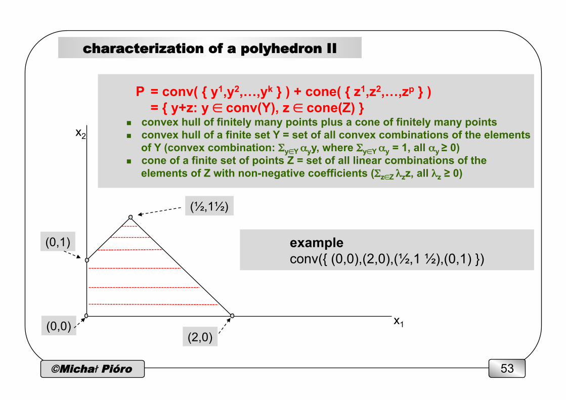
characterization of a polyhedron II
x2
x1
(½,1½)
(0,1)
(2,0) (0,0)
P = conv( { y1,y2,…,yk } ) + cone( { z1,z2,…,zp } ) = { y+z: y ∈ conv(Y), z ∈ cone(Z) }
n convex hull of finitely many points plus a cone of finitely many points n convex hull of a finite set Y = set of all convex combinations of the elements
of Y (convex combination: Σy∈Y αyy, where Σy∈Y αy = 1, all αy ≥ 0) n cone of a finite set of points Z = set of all linear combinations of the
elements of Z with non-negative coefficients (Σz∈Z λzz, all λz ≥ 0)
example conv({ (0,0),(2,0),(½,1 ½),(0,1) })
©Michał Pióro 54
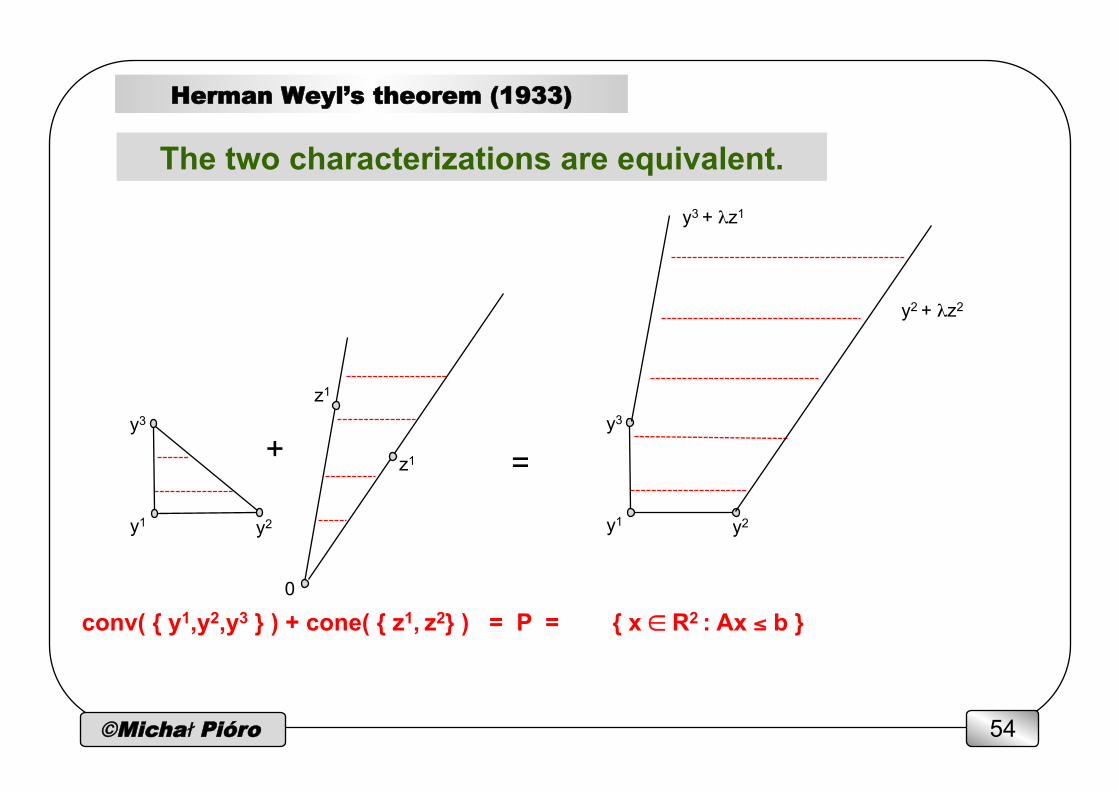
Herman Weyl’s theorem (1933)
The two characterizations are equivalent.
y1
y3
y2
= z1
z1
0
+
y1
y3
y2
y3 + λz1
y2 + λz2
conv( { y1,y2,y3 } ) + cone( { z1, z2} ) = P = { x ∈ R2 : Ax ≤ b }
©Michał Pióro 55
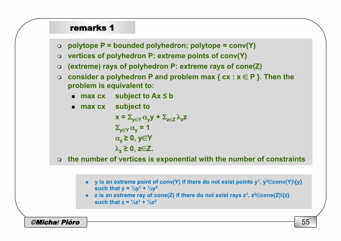
remarks 1
m polytope P = bounded polyhedron; polytope = conv(Y) m vertices of polyhedron P: extreme points of conv(Y) m (extreme) rays of polyhedron P: extreme rays of cone(Z) m consider a polyhedron P and problem max { cx : x ∈ P }. Then the
problem is equivalent to: n max cx subject to Ax ≤ b n max cx subject to
x = Σy∈Y αyy + Σz∈Z λzz Σy∈Y αy = 1 αy ≥ 0, y∈Y λz ≥ 0, z∈Z.
m the number of vertices is exponential with the number of constraints
n y is an extreme point of conv(Y) if there do not exist points y1, y2∈conv(Y)\{y} such that y = ½y1 + ½y2
n z is an extreme ray of cone(Z) if there do not exist rays z1, z2∈cone(Z)\{z} such that z = ½z1 + ½z2
©Michał Pióro 56
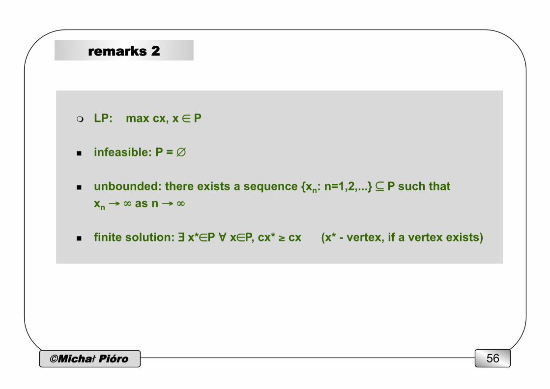
remarks 2
m LP: max cx, x ∈ P
n infeasible: P = ∅
n unbounded: there exists a sequence {xn: n=1,2,...} ⊆ P such that xn → ∞ as n → ∞
n finite solution: ∃ x*∈P ∀ x∈P, cx* ≥ cx (x* - vertex, if a vertex exists)
©Michał Pióro 57
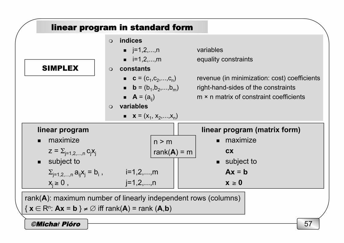
linear program in standard form
m indices n j=1,2,...,n variables n i=1,2,...,m equality constraints
m constants n c = (c1,c2,...,cn) revenue (in minimization: cost) coefficients n b = (b1,b2,...,bm) right-hand-sides of the constraints n A = (aij) m × n matrix of constraint coefficients
m variables n x = (x1, x2,...,xn)
linear program n maximize
z = Σj=1,2,...,n cjxj n subject to
Σj=1,2,...,n aijxj = bi , i=1,2,...,m xj ≥ 0 , j=1,2,...,n
linear program (matrix form) n maximize
cx n subject to
Ax = b x ≥ 0
n > m rank(A) = m
SIMPLEX
rank(A): maximum number of linearly independent rows (columns) { x ∈ Rn: Ax = b } ≠ ∅ iff rank(A) = rank (A,b)
©Michał Pióro 58
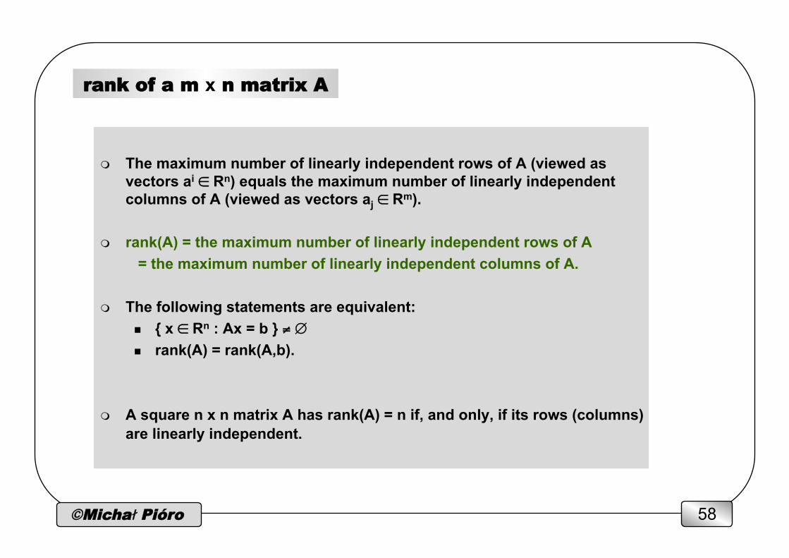
rank of a m x n matrix A
m The maximum number of linearly independent rows of A (viewed as vectors ai ∈ Rn) equals the maximum number of linearly independent columns of A (viewed as vectors aj ∈ Rm).
m rank(A) = the maximum number of linearly independent rows of A = the maximum number of linearly independent columns of A.
m The following statements are equivalent: n { x ∈ Rn : Ax = b } ≠ ∅ n rank(A) = rank(A,b).
m A square n x n matrix A has rank(A) = n if, and only, if its rows (columns) are linearly independent.
©Michał Pióro 59
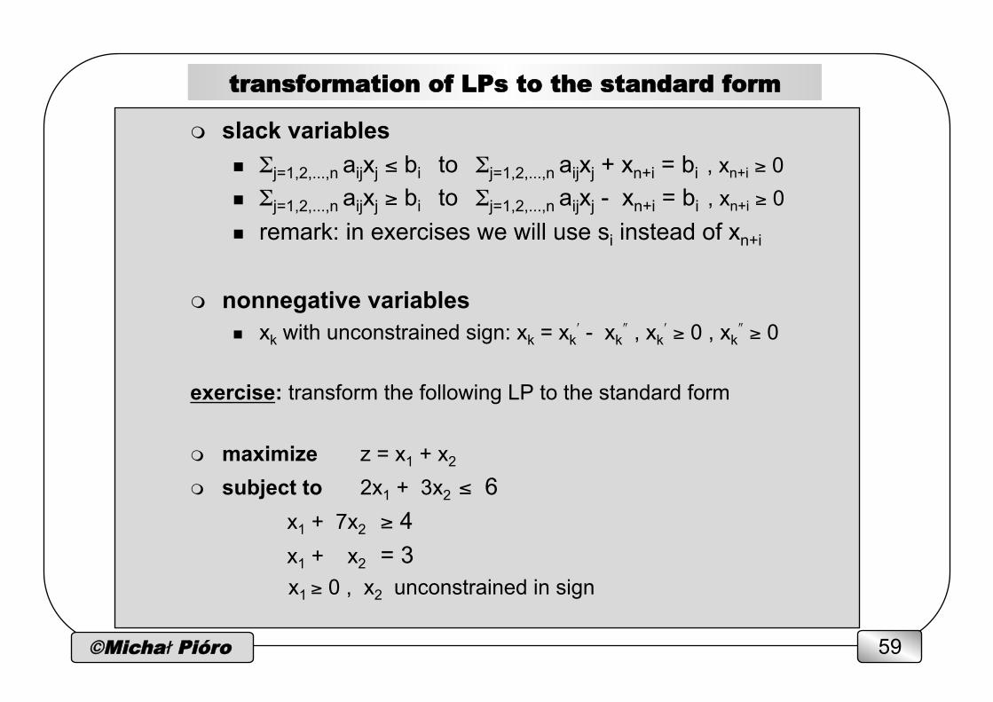
transformation of LPs to the standard form
m slack variables n Σj=1,2,...,n aijxj ≤ bi to Σj=1,2,...,n aijxj + xn+i = bi , xn+i ≥ 0 n Σj=1,2,...,n aijxj ≥ bi to Σj=1,2,...,n aijxj - xn+i = bi , xn+i ≥ 0 n remark: in exercises we will use si instead of xn+i
m nonnegative variables n xk with unconstrained sign: xk = xk
ʹ′ - xkʺ″ , xk
ʹ′ ≥ 0 , xkʺ″ ≥ 0
exercise: transform the following LP to the standard form m maximize z = x1 + x2 m subject to 2x1 + 3x2 ≤ 6
x1 + 7x2 ≥ 4
x1 + x2 = 3 x1 ≥ 0 , x2 unconstrained in sign

©Michał Pióro 60
Basic facts of Linear Programming
m feasible solution - satisfying constraints m basis matrix - a non-singular m × m submatrix of A m basic solution to a LP - the unique vector determined by a basis matrix: n-m
variables associated with columns of A not in the basis matrix are set to 0, and the remaining m variables result from the square system of equations
m basic feasible solution - basic solution with all variables nonnegative (at most m variables can be positive)
m Theorem 1
A vector x = (x1, x2,...,xn) is an extreme point of the constraint set if and only if x is a basic feasible solution.
m Theorem 2 The objective function, z, assumes its maximum at an extreme point of the constraint set.
standard form
To find the optimum: (efficient?) generate all basis matrices and find the best basic feasible solution.
©Michał Pióro 61
basic solutions
A :
a(j1) a(j2) a(jm)
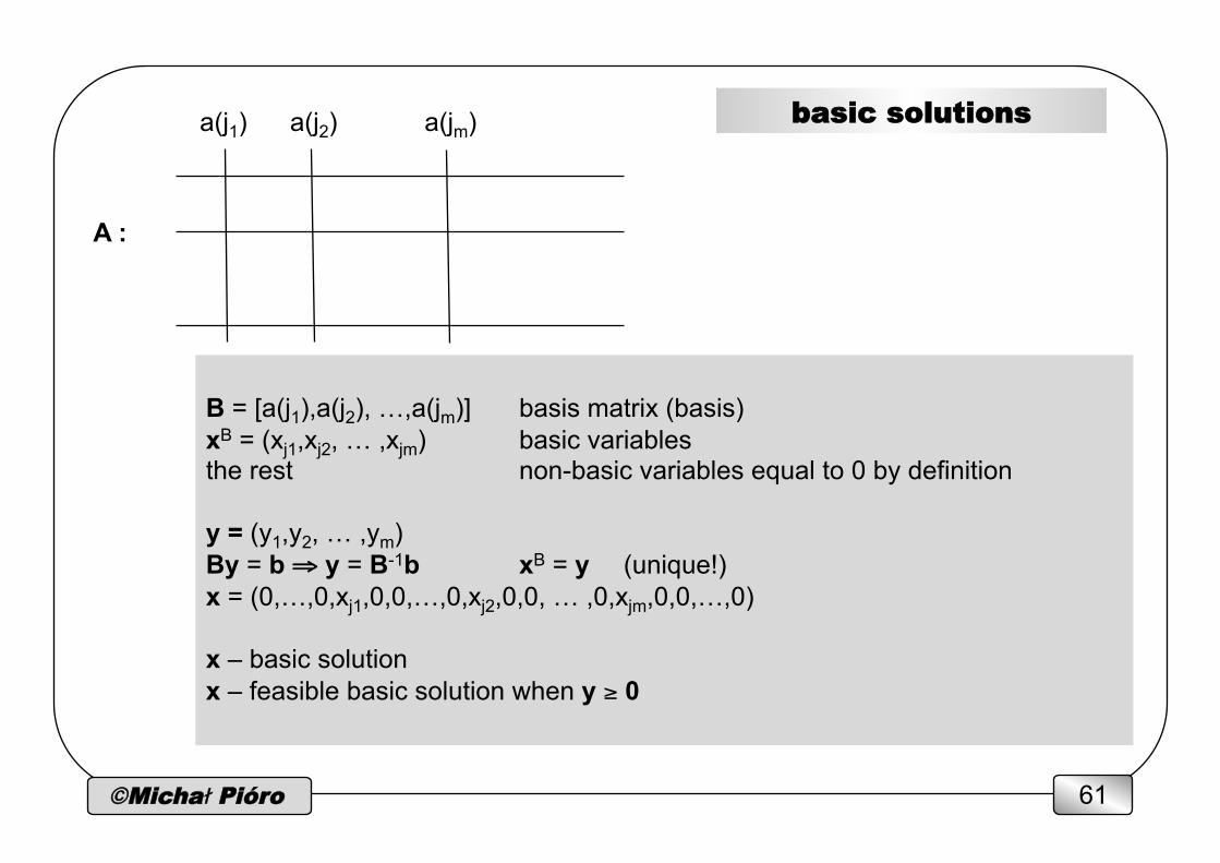
B = [a(j1),a(j2), …,a(jm)] basis matrix (basis) xB = (xj1,xj2, … ,xjm) basic variables the rest non-basic variables equal to 0 by definition y = (y1,y2, … ,ym) By = b ⇒ y = B-1b xB = y (unique!) x = (0,…,0,xj1,0,0,…,0,xj2,0,0, … ,0,xjm,0,0,…,0) x – basic solution x – feasible basic solution when y ≥ 0
©Michał Pióro 62
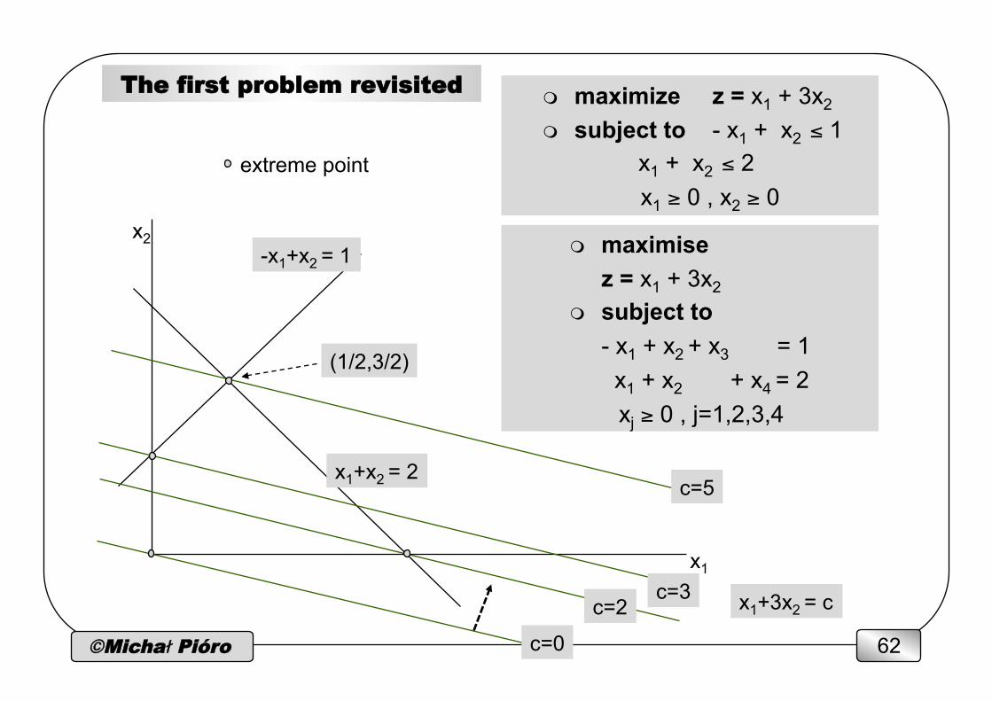
The first problem revisited m maximize z = x1 + 3x2 m subject to - x1 + x2 ≤ 1
x1 + x2 ≤ 2 x1 ≥ 0 , x2 ≥ 0
x2
x1
-x1+x2 = 1
x1+x2 = 2
x1+3x2 = c
c=5
c=3
c=0
(1/2,3/2)
extreme point
m maximise z = x1 + 3x2
m subject to - x1 + x2 + x3 = 1 x1 + x2 + x4 = 2 xj ≥ 0 , j=1,2,3,4
c=2
©Michał Pióro 63
the first problem revisited cntd.
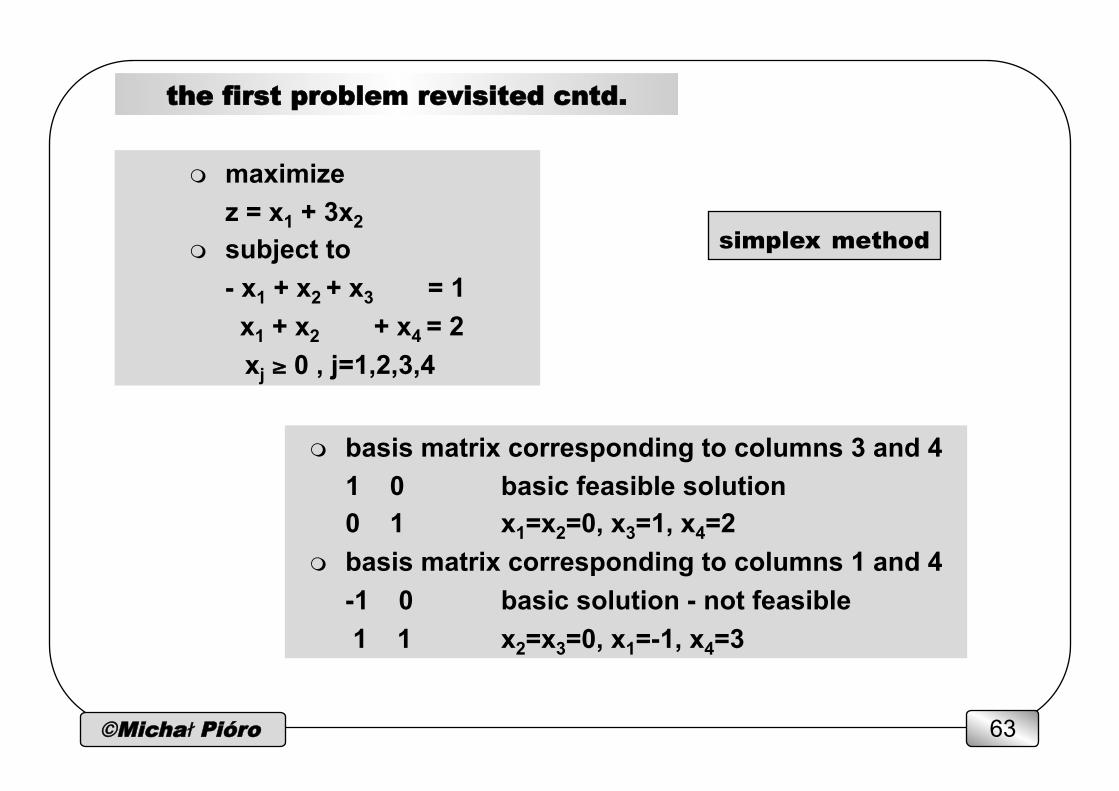
m maximize z = x1 + 3x2
m subject to - x1 + x2 + x3 = 1 x1 + x2 + x4 = 2 xj ≥ 0 , j=1,2,3,4
m basis matrix corresponding to columns 3 and 4 1 0 basic feasible solution 0 1 x1=x2=0, x3=1, x4=2
m basis matrix corresponding to columns 1 and 4 -1 0 basic solution - not feasible 1 1 x2=x3=0, x1=-1, x4=3
simplex method
©Michał Pióro 64
simplex method
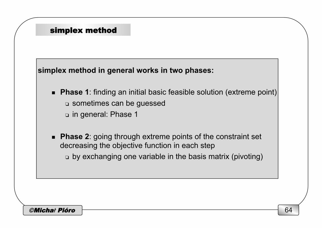
simplex method in general works in two phases:
n Phase 1: finding an initial basic feasible solution (extreme point) ❏ sometimes can be guessed ❏ in general: Phase 1
n Phase 2: going through extreme points of the constraint set
decreasing the objective function in each step ❏ by exchanging one variable in the basis matrix (pivoting)
©Michał Pióro 65
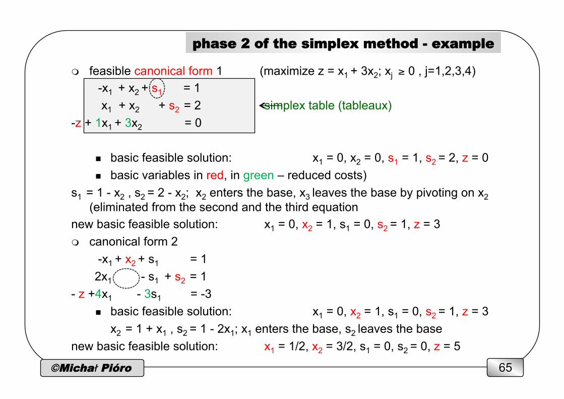
m feasible canonical form 1 (maximize z = x1 + 3x2; xj ≥ 0 , j=1,2,3,4) -x1 + x2 + s1 = 1 x1 + x2 + s2 = 2 simplex table (tableaux)
-z + 1x1 + 3x2 = 0
n basic feasible solution: x1 = 0, x2 = 0, s1 = 1, s2 = 2, z = 0 n basic variables in red, in green – reduced costs)
s1 = 1 - x2 , s2 = 2 - x2; x2 enters the base, x3 leaves the base by pivoting on x2 (eliminated from the second and the third equation
new basic feasible solution: x1 = 0, x2 = 1, s1 = 0, s2 = 1, z = 3 m canonical form 2 -x1 + x2 + s1 = 1 2x1 - s1 + s2 = 1 - z +4x1 - 3s1 = -3
n basic feasible solution: x1 = 0, x2 = 1, s1 = 0, s2 = 1, z = 3 x2 = 1 + x1 , s2 = 1 - 2x1; x1 enters the base, s2 leaves the base
new basic feasible solution: x1 = 1/2, x2 = 3/2, s1 = 0, s2 = 0, z = 5
phase 2 of the simplex method - example
©Michał Pióro 66
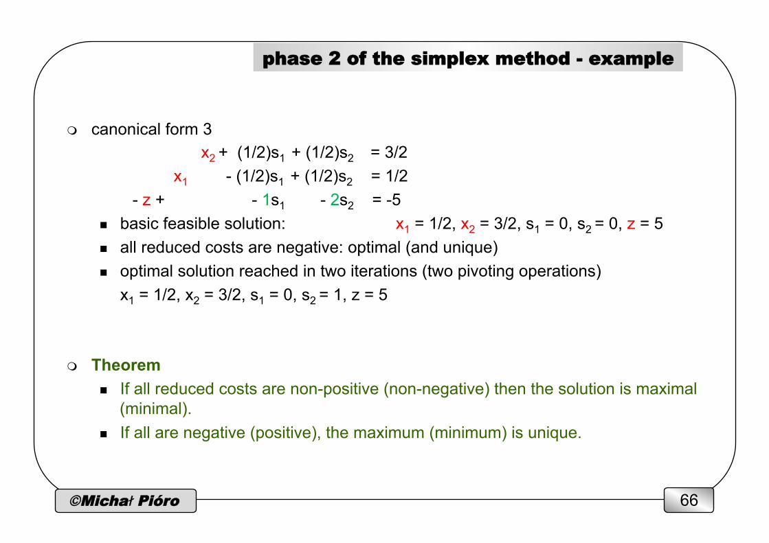
m canonical form 3 x2 + (1/2)s1 + (1/2)s2 = 3/2 x1 - (1/2)s1 + (1/2)s2 = 1/2
- z + - 1s1 - 2s2 = -5 n basic feasible solution: x1 = 1/2, x2 = 3/2, s1 = 0, s2 = 0, z = 5 n all reduced costs are negative: optimal (and unique) n optimal solution reached in two iterations (two pivoting operations)
x1 = 1/2, x2 = 3/2, s1 = 0, s2 = 1, z = 5
m Theorem n If all reduced costs are non-positive (non-negative) then the solution is maximal
(minimal). n If all are negative (positive), the maximum (minimum) is unique.
phase 2 of the simplex method - example
©Michał Pióro 67
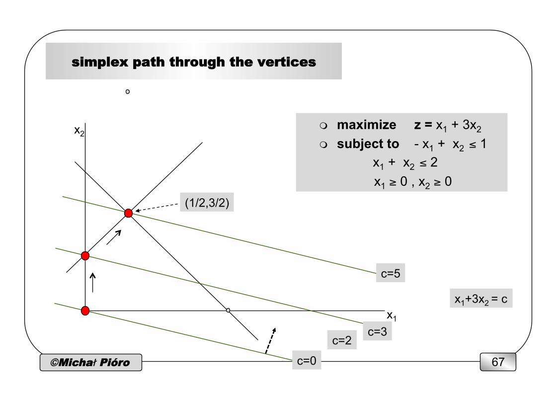
simplex path through the vertices
m maximize z = x1 + 3x2 m subject to - x1 + x2 ≤ 1
x1 + x2 ≤ 2 x1 ≥ 0 , x2 ≥ 0
x2
x1
x1+3x2 = c
c=5
c=3
c=0
(1/2,3/2)
c=2
©Michał Pióro 68
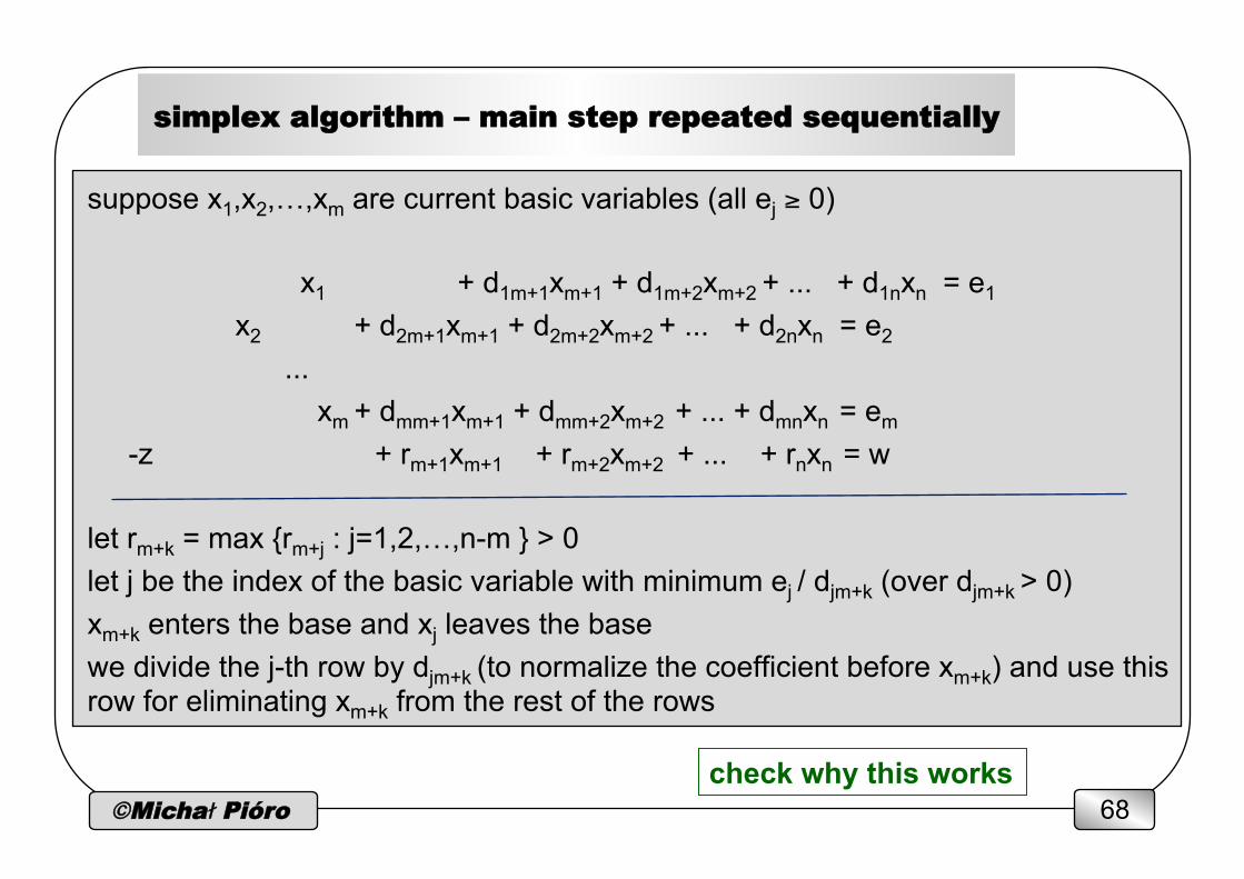
simplex algorithm – main step repeated sequentially
suppose x1,x2,…,xm are current basic variables (all ej ≥ 0)
x1 + d1m+1xm+1 + d1m+2xm+2 + ... + d1nxn = e1 x2 + d2m+1xm+1 + d2m+2xm+2 + ... + d2nxn = e2
... xm + dmm+1xm+1 + dmm+2xm+2 + ... + dmnxn = em
-z + rm+1xm+1 + rm+2xm+2 + ... + rnxn = w
let rm+k = max {rm+j : j=1,2,…,n-m } > 0 let j be the index of the basic variable with minimum ej / djm+k (over djm+k > 0) xm+k enters the base and xj leaves the base we divide the j-th row by djm+k (to normalize the coefficient before xm+k) and use this row for eliminating xm+k from the rest of the rows
check why this works
©Michał Pióro 69
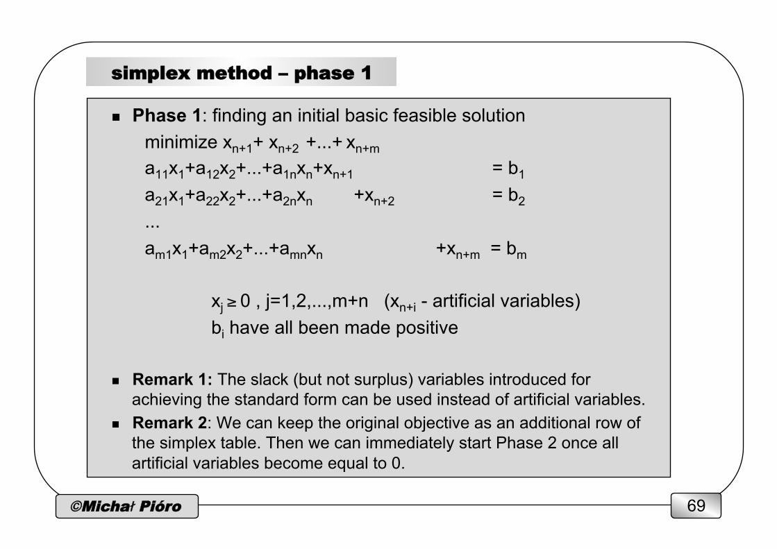
simplex method – phase 1
n Phase 1: finding an initial basic feasible solution minimize xn+1+ xn+2 +...+ xn+m a11x1+a12x2+...+a1nxn+xn+1 = b1 a21x1+a22x2+...+a2nxn +xn+2 = b2
... am1x1+am2x2+...+amnxn +xn+m = bm
xj ≥ 0 , j=1,2,...,m+n (xn+i - artificial variables)
bi have all been made positive n Remark 1: The slack (but not surplus) variables introduced for
achieving the standard form can be used instead of artificial variables. n Remark 2: We can keep the original objective as an additional row of
the simplex table. Then we can immediately start Phase 2 once all artificial variables become equal to 0.
©Michał Pióro 70
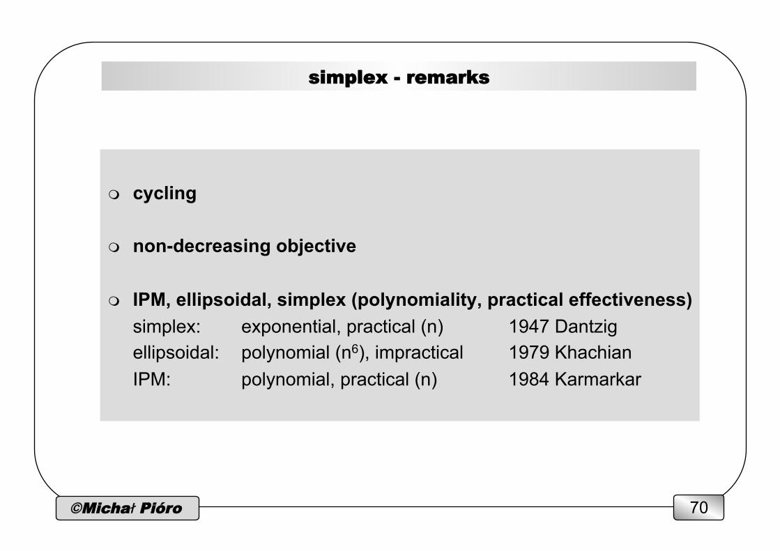
simplex - remarks
m cycling
m non-decreasing objective
m IPM, ellipsoidal, simplex (polynomiality, practical effectiveness) simplex: exponential, practical (n) 1947 Dantzig ellipsoidal: polynomial (n6), impractical 1979 Khachian IPM: polynomial, practical (n) 1984 Karmarkar
©Michał Pióro 71
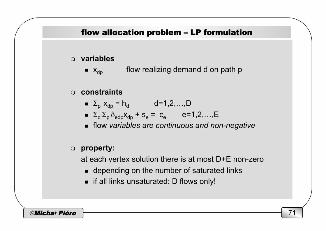
flow allocation problem – LP formulation
m variables n xdp flow realizing demand d on path p
m constraints n Σp xdp = hd d=1,2,…,D n Σd Σp δedpxdp + se = ce e=1,2,…,E n flow variables are continuous and non-negative
m property: at each vertex solution there is at most D+E non-zero
n depending on the number of saturated links n if all links unsaturated: D flows only!
©Michał Pióro 72
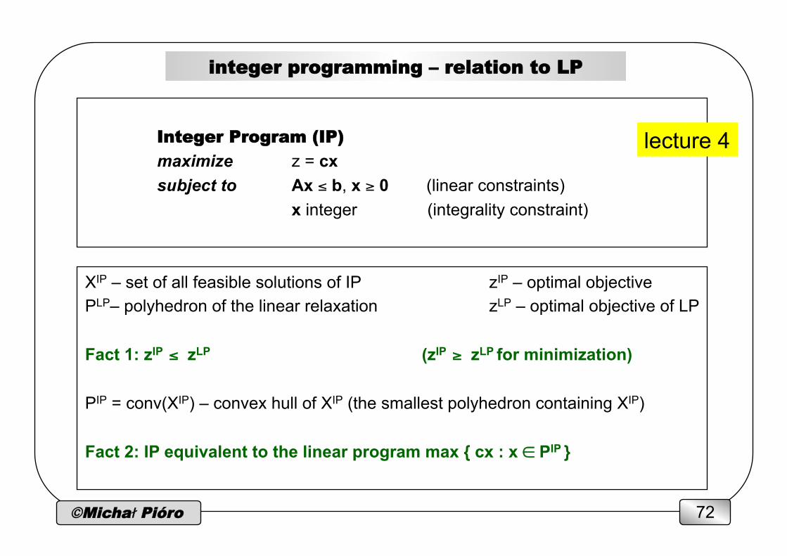
integer programming – relation to LP
Integer Program (IP) maximize z = cx subject to Ax ≤ b, x ≥ 0 (linear constraints)
x integer (integrality constraint)
XIP – set of all feasible solutions of IP zIP – optimal objective PLP– polyhedron of the linear relaxation zLP – optimal objective of LP Fact 1: zIP ≤ zLP (zIP ≥ zLP for minimization) PIP = conv(XIP) – convex hull of XIP (the smallest polyhedron containing XIP) Fact 2: IP equivalent to the linear program max { cx : x ∈ PIP }
lecture 4
©Michał Pióro 73
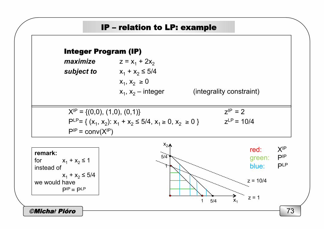
IP – relation to LP: example
XIP = {(0,0), (1,0), (0,1)} zIP = 2 PLP = { (x1, x2): x1 + x2 ≤ 5/4, x1 ≥ 0, x2 ≥ 0 } zLP = 10/4 PIP = conv(XIP)
Integer Program (IP) maximize z = x1 + 2x2 subject to x1 + x2 ≤ 5/4
x1, x2 ≥ 0 x1, x2 – integer (integrality constraint)
5/4 1
1
5/4 red: XIP
green: PIP
blue: PLP
z = 1
z = 10/4
x1
x2
remark: for x1 + x2 ≤ 1 instead of x1 + x2 ≤ 5/4 we would have
PIP = PLP
©Michał Pióro 74
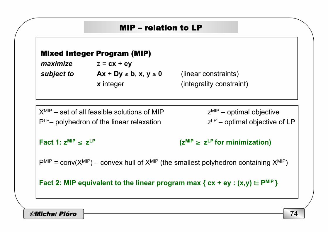
MIP – relation to LP
XMIP – set of all feasible solutions of MIP zMIP – optimal objective PLP– polyhedron of the linear relaxation zLP – optimal objective of LP Fact 1: zMIP ≤ zLP (zMIP ≥ zLP for minimization) PMIP = conv(XMIP) – convex hull of XMIP (the smallest polyhedron containing XMIP) Fact 2: MIP equivalent to the linear program max { cx + ey : (x,y) ∈ PMIP }
Mixed Integer Program (MIP)
maximize z = cx + ey subject to Ax + Dy ≤ b, x, y ≥ 0 (linear constraints)
x integer (integrality constraint)
©Michał Pióro 75
MIP – relation to LP: example
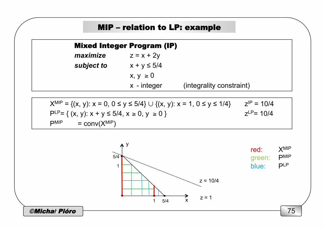
XMIP = {(x, y): x = 0, 0 ≤ y ≤ 5/4} ∪ {(x, y): x = 1, 0 ≤ y ≤ 1/4} zIP = 10/4 PLP = { (x, y): x + y ≤ 5/4, x ≥ 0, y ≥ 0 } zLP= 10/4 PMIP = conv(XMIP)
Mixed Integer Program (IP) maximize z = x + 2y subject to x + y ≤ 5/4
x, y ≥ 0 x - integer (integrality constraint)
5/4 1
1
5/4 red: XMIP
green: PMIP
blue: PLP
z = 1
z = 10/4
x
y
©Michał Pióro 76
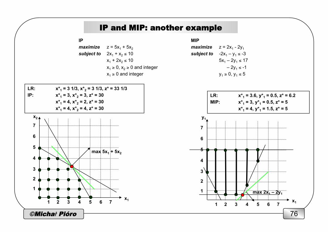
IP and MIP: another example
IP MIP maximize z = 5x1 + 5x2 maximize z = 2x1 - 2y1 subject to 2x1 + x2 ≤ 10 subject to -2x1 – y1 ≤ -3
x1 + 2x2 ≤ 10 5x1 – 2y1 ≤ 17 x1 ≥ 0, x2 ≥ 0 and integer – 2y1 ≤ -1 x1 ≥ 0 and integer y1 ≥ 0, y1 ≤ 5
7
6
5
4
3
2
1
6 7 5 4 3 2 1
7
6
5
4
3
2
1
6 7 5 4 3 2 1
max 5x1 + 5x2
max 2x1 – 2y1
x1
x2 y1
x1
LR: x*1 = 3.6, y*1 = 0.5, z* = 6.2 MIP: x*1 = 3, y*1 = 0.5, z* = 5
x*1 = 4, y*1 = 1.5, z* = 5
LR: x*1 = 3 1/3, x*2 = 3 1/3, z* = 33 1/3 IP: x*1 = 3, x*2 = 3, z* = 30
x*1 = 4, x*2 = 2, z* = 30 x*1 = 4, x*2 = 4, z* = 30
©Michał Pióro 77
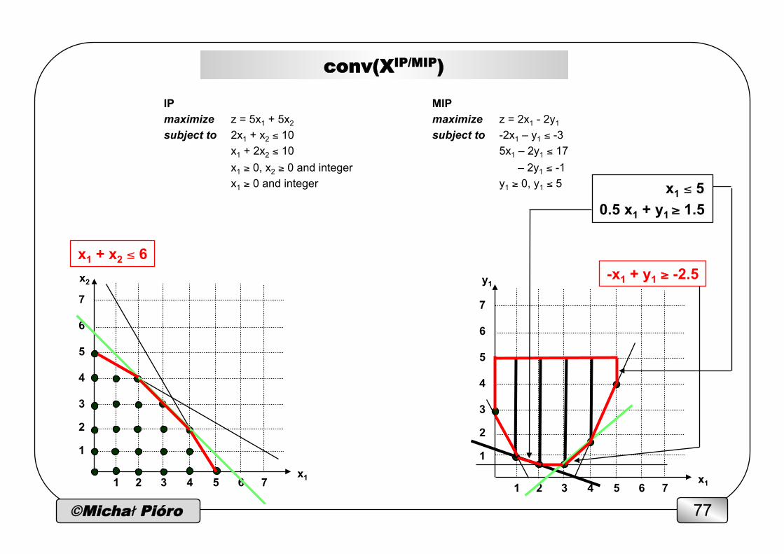
conv(XIP/MIP)
7
6
5
4
3
2
1
6 7 5 4 3 2 1
7
6
5
4
3
2
1
6 7 5 4 3 2 1 x1
x2 y1
x1
-x1 + y1 ≥ -2.5 x1 + x2 ≤ 6
IP MIP maximize z = 5x1 + 5x2 maximize z = 2x1 - 2y1 subject to 2x1 + x2 ≤ 10 subject to -2x1 – y1 ≤ -3
x1 + 2x2 ≤ 10 5x1 – 2y1 ≤ 17 x1 ≥ 0, x2 ≥ 0 and integer – 2y1 ≤ -1 x1 ≥ 0 and integer y1 ≥ 0, y1 ≤ 5
x1 ≤ 5 0.5 x1 + y1 ≥ 1.5
©Michał Pióro 78
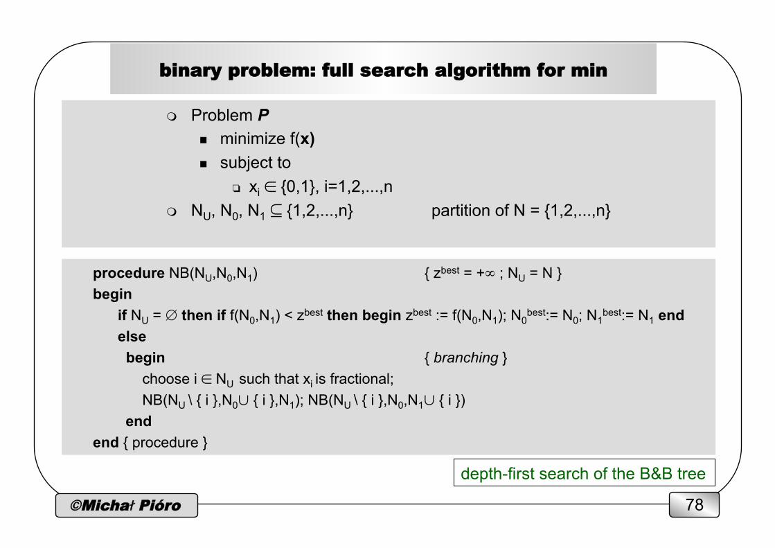
binary problem: full search algorithm for min
procedure NB(NU,N0,N1) { zbest = +∞ ; NU = N } begin
if NU = ∅ then if f(N0,N1) < zbest then begin zbest := f(N0,N1); N0best:= N0; N1
best:= N1 end else begin { branching } choose i ∈ NU such that xi is fractional; NB(NU \ { i },N0∪ { i },N1); NB(NU \ { i },N0,N1∪ { i })
end end { procedure }
depth-first search of the B&B tree
m Problem P n minimize f(x) n subject to
❏ xi ∈ {0,1}, i=1,2,...,n m NU, N0, N1 ⊆ {1,2,...,n} partition of N = {1,2,...,n}
©Michał Pióro 79
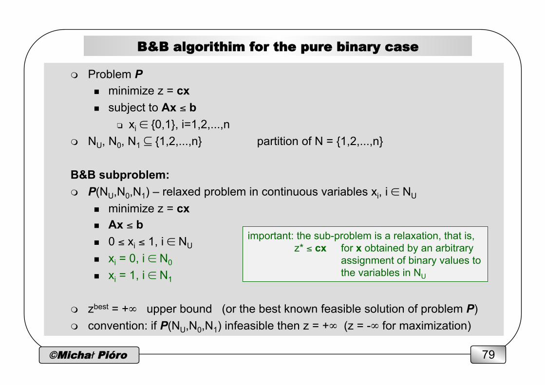
B&B algorithim for the pure binary case
m Problem P n minimize z = cx n subject to Ax ≤ b
❏ xi ∈ {0,1}, i=1,2,...,n m NU, N0, N1 ⊆ {1,2,...,n} partition of N = {1,2,...,n}
B&B subproblem: m P(NU,N0,N1) – relaxed problem in continuous variables xi, i ∈ NU
n minimize z = cx n Ax ≤ b n 0 ≤ xi ≤ 1, i ∈ NU
n xi = 0, i ∈ N0
n xi = 1, i ∈ N1
m zbest = +∞ upper bound (or the best known feasible solution of problem P) m convention: if P(NU,N0,N1) infeasible then z = +∞ (z = -∞ for maximization)
important: the sub-problem is a relaxation, that is, z* ≤ cx for x obtained by an arbitrary assignment of binary values to the variables in NU

©Michał Pióro 80
B&B for the pure binary case – algorithm for min
procedure BBB(NU,N0,N1) { zbest = +∞ } begin
solution(NU,N0,N1,x,z); { solve P(NU,N0,N1) } if NU = ∅ or for all i ∈ NU xi are binary then if z < zbest then begin zbest := z; xbest := x end else if z ≥ zbest then return { bounding } else begin { branching } choose i ∈ NU such that xi is fractional; BBB(NU \ { i },N0∪ { i },N1); BBB(NU \ { i },N0,N1∪ { i }) end
end { procedure }
depth-first search of the B&B tree

©Michał Pióro 81
single-path allocation problem – MIP formulation
m variables n udp binary flow realizing demand d on path p
m minimize z
m constraints n Σp udp = 1 d=1,2,…,D n Σd Σp δedphdudp ≤ ce + z e=1,2,…,E
in the optimum: z = max{ Σd Σp δedphdudp - ce } i.e., integer when h and c integer

©Michał Pióro 82
B&B – example (depth-first)
c=0 c=4
c=9
h1=10 h2=4
all relaxed z = 1/3
u11=1/30, u12=28/30, u13=1/30 u21=0, u22=0, u23=1
u11=0 z = 1/3
u11=1 z = 10
u11=0, u12=0 z = 6 (integer)
u11=0, u12=1 z = 1 (int. opt.)
u11=0, u12=0, u13=1 u21=0, u22=1, u23=0
u11=0, u12=1, u13=0 u21=0, u22=0, u23=1
No need to consider when integrality of z is exploited!
©Michał Pióro 83
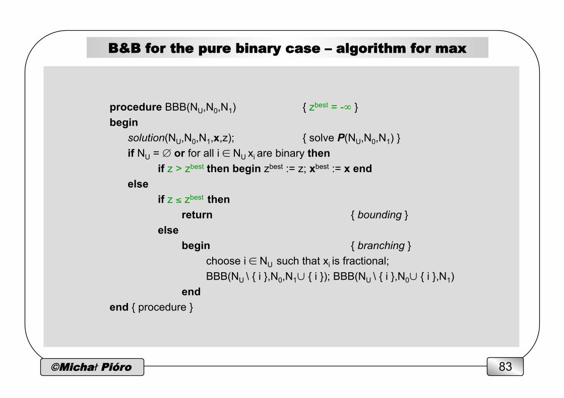
B&B for the pure binary case – algorithm for max
procedure BBB(NU,N0,N1) { zbest = -∞ } begin
solution(NU,N0,N1,x,z); { solve P(NU,N0,N1) } if NU = ∅ or for all i ∈ NU xi are binary then if z > zbest then begin zbest := z; xbest := x end else if z ≤ zbest then return { bounding } else begin { branching } choose i ∈ NU such that xi is fractional; BBB(NU \ { i },N0,N1∪ { i }); BBB(NU \ { i },N0∪ { i },N1) end
end { procedure }
©Michał Pióro 84
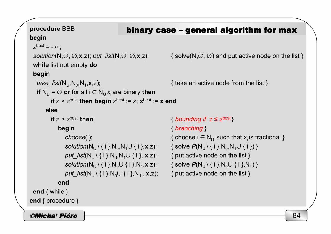
procedure BBB begin zbest = -∞ ; solution(N,∅, ∅,x,z); put_list(N,∅, ∅,x,z); { solve(N,∅, ∅) and put active node on the list } while list not empty do begin take_list(NU,N0,N1,x,z); { take an active node from the list } if NU = ∅ or for all i ∈ NU xi are binary then
if z > zbest then begin zbest := z; xbest := x end else if z > zbest then { bounding if z ≤ zbest } begin { branching } choose(i); { choose i ∈ NU such that xi is fractional } solution(NU \ { i },N0,N1∪ { i },x,z); { solve P(NU \ { i },N0,N1∪ { i }) } put_list(NU \ { i },N0,N1∪ { i }, x,z); { put active node on the list } solution(NU \ { i },N0∪ { i },N1,x,z); { solve P(NU \ { i },N0∪ { i },N1) } put_list(NU \ { i },N0∪ { i },N1 , x,z); { put active node on the list } end
end { while } end { procedure }
binary case – general algorithm for max
©Michał Pióro 85
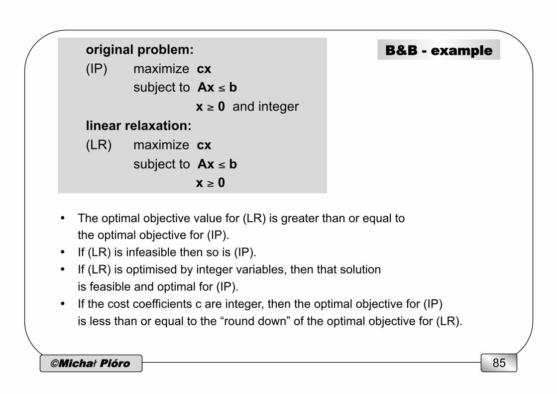
original problem: (IP) maximize cx
subject to Ax ≤ b x ≥ 0 and integer
linear relaxation: (LR) maximize cx
subject to Ax ≤ b x ≥ 0
B&B - example
• The optimal objective value for (LR) is greater than or equal to the optimal objective for (IP).
• If (LR) is infeasible then so is (IP). • If (LR) is optimised by integer variables, then that solution
is feasible and optimal for (IP). • If the cost coefficients c are integer, then the optimal objective for (IP)
is less than or equal to the “round down” of the optimal objective for (LR).
©Michał Pióro 86
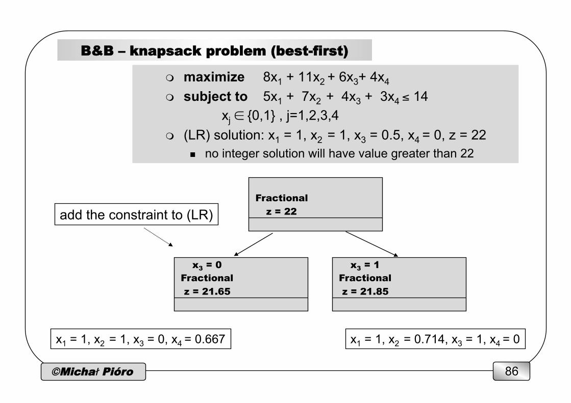
B&B – knapsack problem (best-first)
m maximize 8x1 + 11x2 + 6x3+ 4x4 m subject to 5x1 + 7x2 + 4x3 + 3x4 ≤ 14
xj ∈ {0,1} , j=1,2,3,4
m (LR) solution: x1 = 1, x2 = 1, x3 = 0.5, x4 = 0, z = 22 n no integer solution will have value greater than 22
Fractional
z = 22
x3 = 0 Fractional
z = 21.65
x3 = 1 Fractional
z = 21.85
add the constraint to (LR)
x1 = 1, x2 = 1, x3 = 0, x4 = 0.667 x1 = 1, x2 = 0.714, x3 = 1, x4 = 0
©Michał Pióro 87
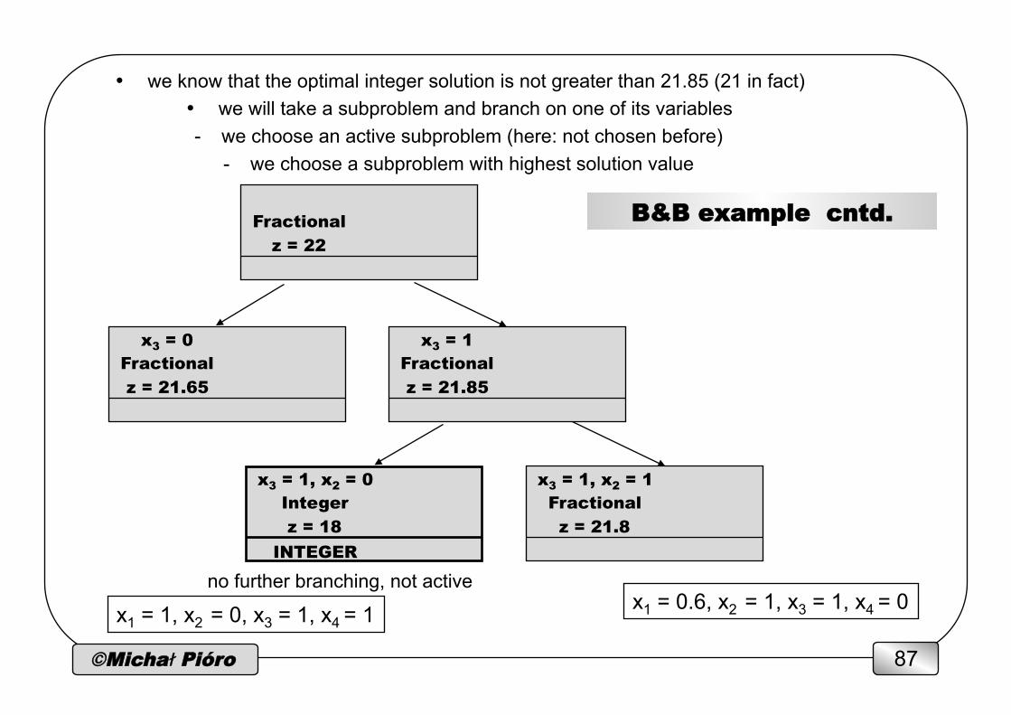
• we know that the optimal integer solution is not greater than 21.85 (21 in fact) • we will take a subproblem and branch on one of its variables - we choose an active subproblem (here: not chosen before)
- we choose a subproblem with highest solution value
B&B example cntd.
Fractional
z = 22
x3 = 0 Fractional
z = 21.65
x3 = 1 Fractional
z = 21.85
x1 = 1, x2 = 0, x3 = 1, x4 = 1 x1 = 0.6, x2 = 1, x3 = 1, x4 = 0
x3 = 1, x2 = 0 Integer
z = 18
INTEGER
x3 = 1, x2 = 1 Fractional
z = 21.8
no further branching, not active
©Michał Pióro 88
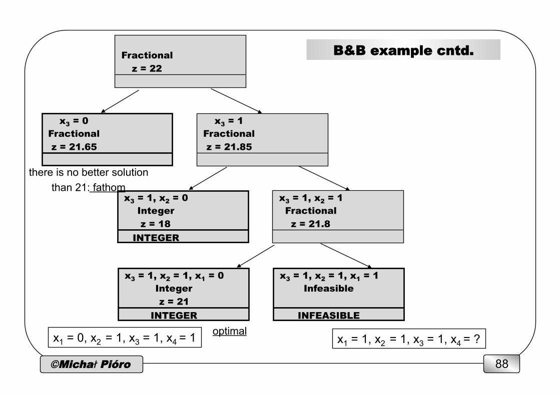
B&B example cntd.
Fractional
z = 22
x3 = 0 Fractional
z = 21.65
x3 = 1 Fractional
z = 21.85
x1 = 0, x2 = 1, x3 = 1, x4 = 1 x1 = 1, x2 = 1, x3 = 1, x4 = ?
x3 = 1, x2 = 0 Integer
z = 18
INTEGER
x3 = 1, x2 = 1 Fractional
z = 21.8
x3 = 1, x2 = 1, x1 = 0 Integer
z = 21
INTEGER
x3 = 1, x2 = 1, x1 = 1 Infeasible
INFEASIBLE
there is no better solution than 21: fathom
optimal
©Michał Pióro 89
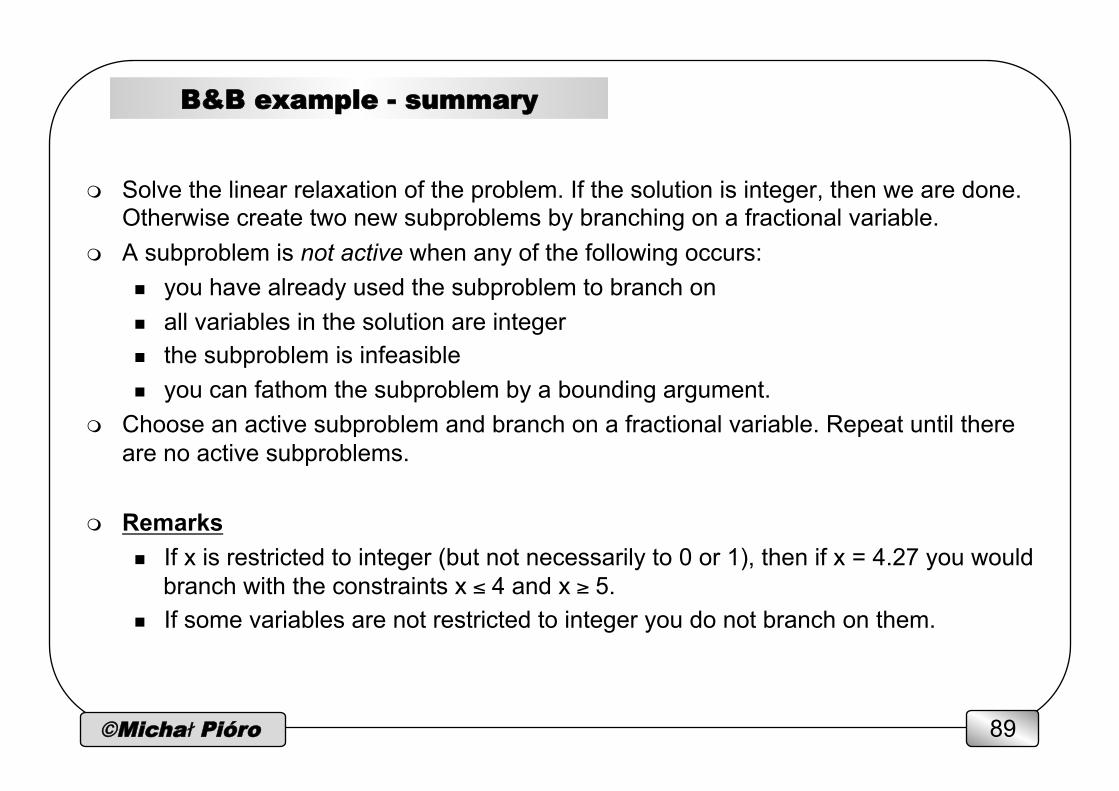
B&B example - summary
m Solve the linear relaxation of the problem. If the solution is integer, then we are done. Otherwise create two new subproblems by branching on a fractional variable.
m A subproblem is not active when any of the following occurs: n you have already used the subproblem to branch on n all variables in the solution are integer n the subproblem is infeasible n you can fathom the subproblem by a bounding argument.
m Choose an active subproblem and branch on a fractional variable. Repeat until there are no active subproblems.
m Remarks
n If x is restricted to integer (but not necessarily to 0 or 1), then if x = 4.27 you would branch with the constraints x ≤ 4 and x ≥ 5.
n If some variables are not restricted to integer you do not branch on them.

©Michał Pióro 90
tree searching and branching strategies
• the order of visiting the nodes of the B&B tree • procedure take: take the first element from the list of active nodes • procedure put: defines the order
• best first: sort by the optimal values of the LR subproblem z • depth-first: put on top of the list (list = stack)
• choose(i) • choose the first fractional variable • choose the one closest to ½ (in the binary case)
• there are no general rules for put and choose
©Michał Pióro 91
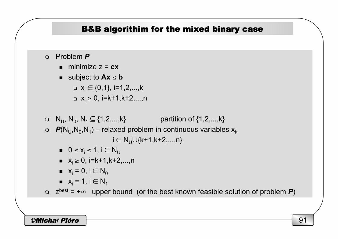
B&B algorithim for the mixed binary case
m Problem P n minimize z = cx n subject to Ax ≤ b
❏ xi ∈ {0,1}, i=1,2,...,k ❏ xi ≥ 0, i=k+1,k+2,...,n
m NU, N0, N1 ⊆ {1,2,...,k} partition of {1,2,...,k} m P(NU,N0,N1) – relaxed problem in continuous variables xi,
i ∈ NU∪{k+1,k+2,...,n} n 0 ≤ xi ≤ 1, i ∈ NU
n xi ≥ 0, i=k+1,k+2,...,n n xi = 0, i ∈ N0
n xi = 1, i ∈ N1
m zbest = +∞ upper bound (or the best known feasible solution of problem P)
©Michał Pióro 92
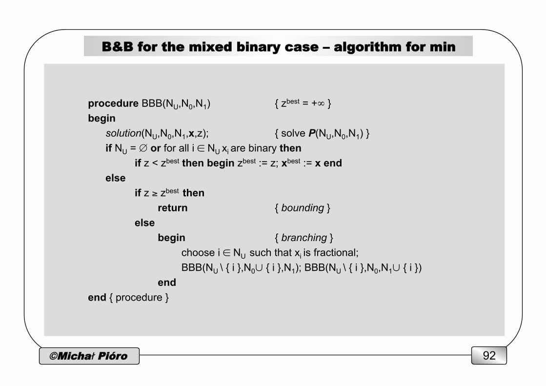
B&B for the mixed binary case – algorithm for min
procedure BBB(NU,N0,N1) { zbest = +∞ } begin
solution(NU,N0,N1,x,z); { solve P(NU,N0,N1) } if NU = ∅ or for all i ∈ NU xi are binary then if z < zbest then begin zbest := z; xbest := x end else if z ≥ zbest then return { bounding } else begin { branching } choose i ∈ NU such that xi is fractional; BBB(NU \ { i },N0∪ { i },N1); BBB(NU \ { i },N0,N1∪ { i }) end
end { procedure }
©Michał Pióro 93
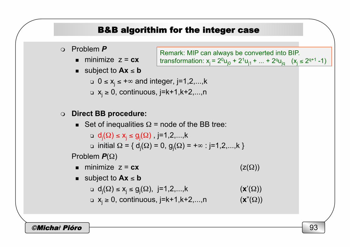
B&B algorithim for the integer case
m Problem P n minimize z = cx n subject to Ax ≤ b
❏ 0 ≤ xj ≤ +∞ and integer, j=1,2,...,k ❏ xj ≥ 0, continuous, j=k+1,k+2,...,n
m Direct BB procedure: n Set of inequalities Ω = node of the BB tree:
❏ dj(Ω) ≤ xj ≤ gj(Ω) , j=1,2,...,k ❏ initial Ω = { dj(Ω) = 0, gj(Ω) = +∞ : j=1,2,...,k }
Problem P(Ω) n minimize z = cx (z(Ω)) n subject to Ax ≤ b
❏ dj(Ω) ≤ xj ≤ gj(Ω), j=1,2,...,k (x’(Ω)) ❏ xj ≥ 0, continuous, j=k+1,k+2,...,n (x”(Ω))
Remark: MIP can always be converted into BIP. transformation: xj = 20uj0 + 21uj1 + ... + 2qujq (xj ≤ 2q+1 -1)
©Michał Pióro 94
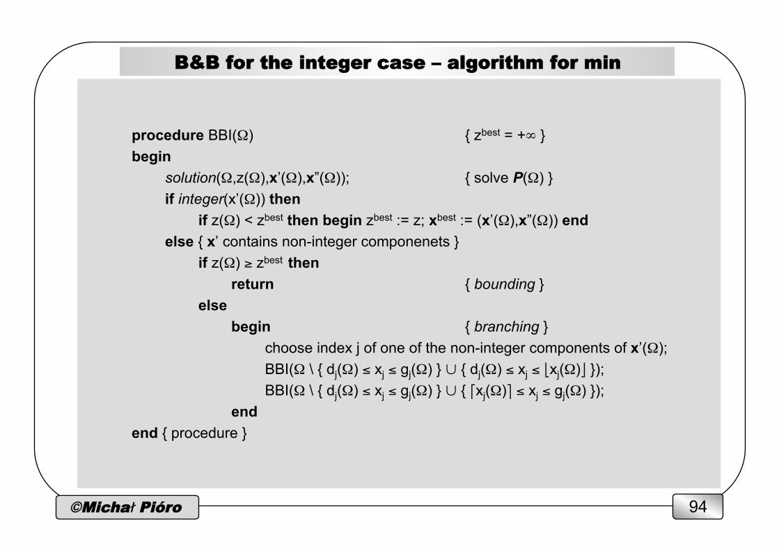
B&B for the integer case – algorithm for min
procedure BBI(Ω) { zbest = +∞ } begin
solution(Ω,z(Ω),x’(Ω),x”(Ω)); { solve P(Ω) } if integer(x’(Ω)) then if z(Ω) < zbest then begin zbest := z; xbest := (x’(Ω),x”(Ω)) end else { x’ contains non-integer componenets } if z(Ω) ≥ zbest then return { bounding } else begin { branching } choose index j of one of the non-integer components of x’(Ω); BBI(Ω \ { dj(Ω) ≤ xj ≤ gj(Ω) } ∪ { dj(Ω) ≤ xj ≤ ⎣xj(Ω)⎦ }); BBI(Ω \ { dj(Ω) ≤ xj ≤ gj(Ω) } ∪ { ⎡xj(Ω)⎤ ≤ xj ≤ gj(Ω) }); end
end { procedure }

©Michał Pióro 95
dimensioning - cases
m objective minimize F(y) = Σe ξeye
n Σd Σp δedpxdp ≤ M⋅ye e=1,2,…,E ye integer MIP n Σd Σp δedpxdp ≤ Σk Mk⋅yek e=1,2,…,E yek integer IP
m objective minimize F(y) = Σe ξef(ye) n ye = Σd Σp δedpxdp n f(z) – convex (penalty, delay) - CXP n f(z) – concave (dimensioning function) - CVP
lecture 5
©Michał Pióro 96
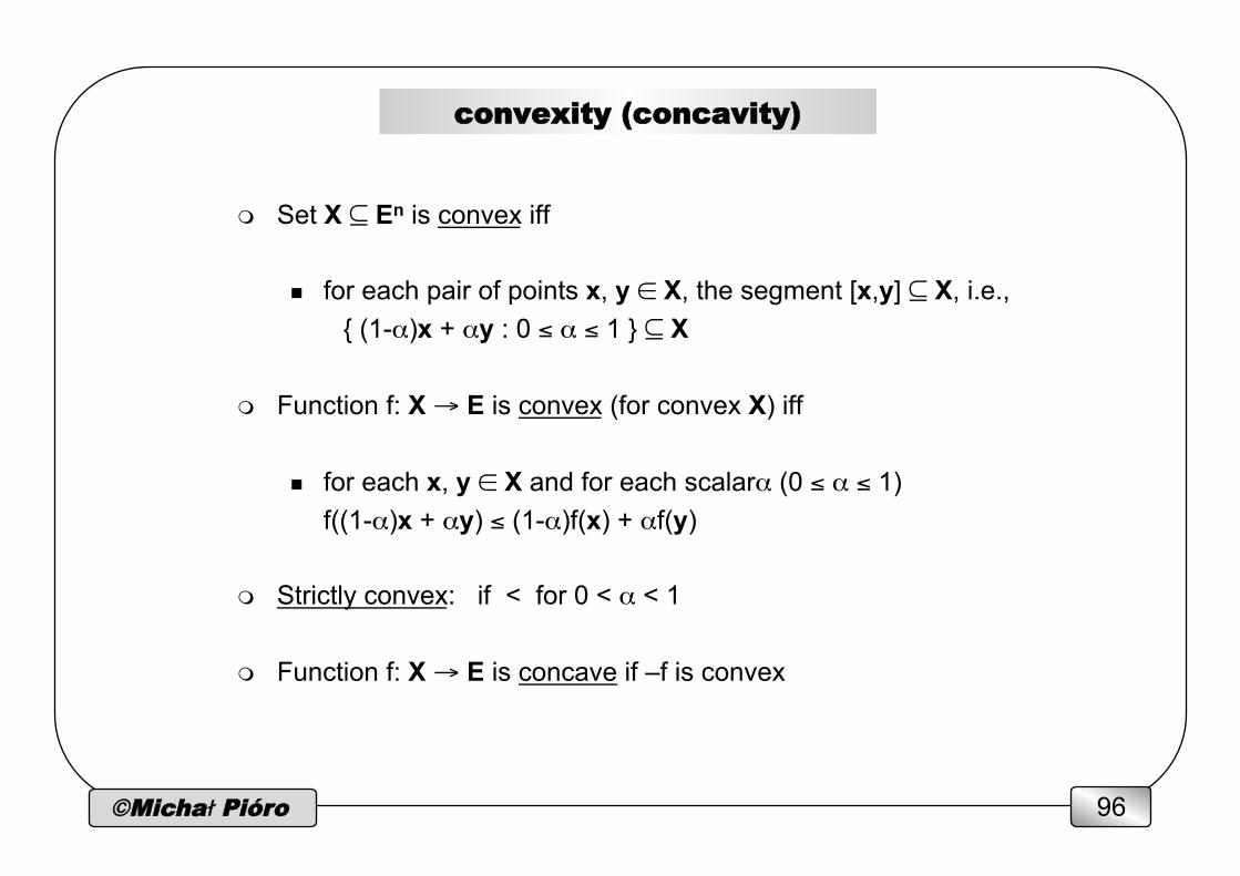
convexity (concavity)
m Set X ⊆ En is convex iff
n for each pair of points x, y ∈ X, the segment [x,y] ⊆ X, i.e., { (1-α)x + αy : 0 ≤ α ≤ 1 } ⊆ X
m Function f: X → E is convex (for convex X) iff
n for each x, y ∈ X and for each scalarα (0 ≤ α ≤ 1) f((1-α)x + αy) ≤ (1-α)f(x) + αf(y)
m Strictly convex: if < for 0 < α < 1
m Function f: X → E is concave if –f is convex
©Michał Pióro 97
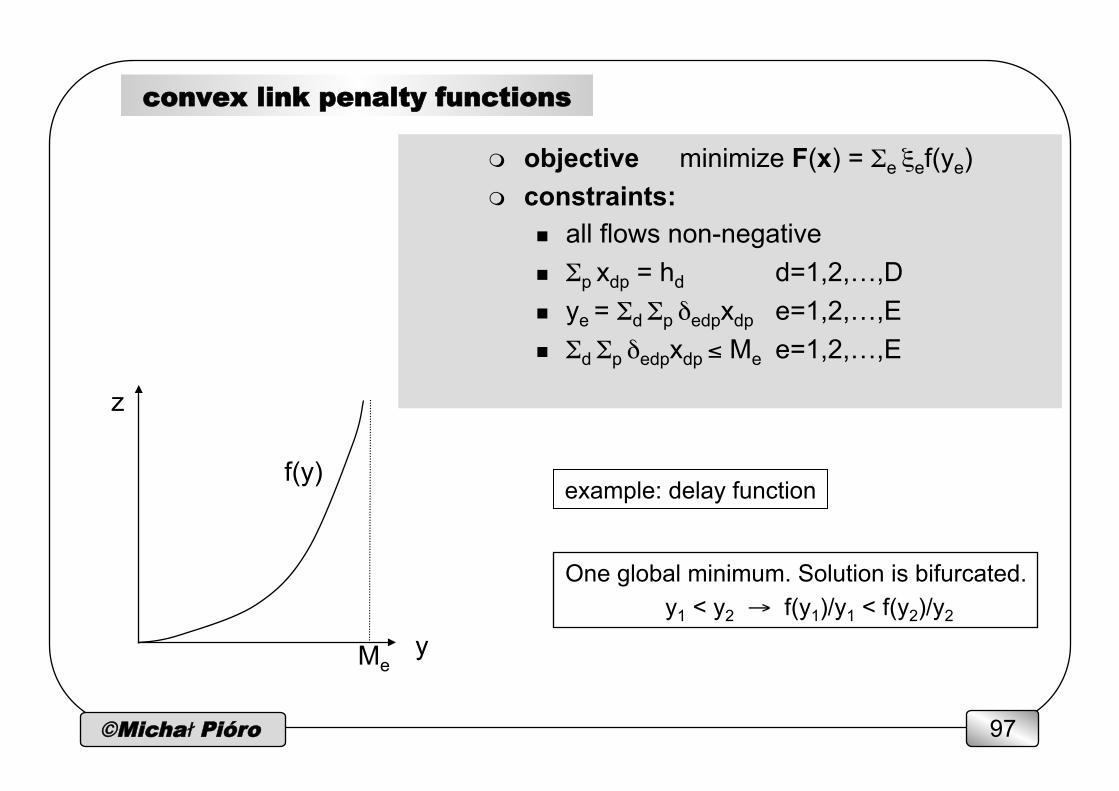
convex link penalty functions
m objective minimize F(x) = Σe ξef(ye) m constraints:
n all flows non-negative n Σp xdp = hd d=1,2,…,D n ye = Σd Σp δedpxdp e=1,2,…,E n Σd Σp δedpxdp ≤ Me e=1,2,…,E
f(y)
y
One global minimum. Solution is bifurcated. y1 < y2 → f(y1)/y1 < f(y2)/y2
Me
z
example: delay function
©Michał Pióro 98
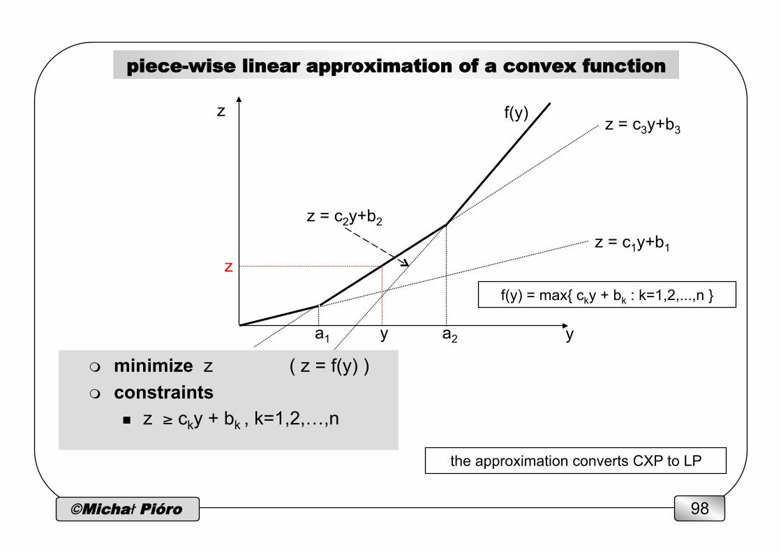
piece-wise linear approximation of a convex function
m minimize z ( z = f(y) ) m constraints
n z ≥ cky + bk , k=1,2,…,n
f(y)
y a1 a2
z = c3y+b3
y
z = c1y+b1
z = c2y+b2
the approximation converts CXP to LP
f(y) = max{ cky + bk : k=1,2,...,n }
z
z
©Michał Pióro 99
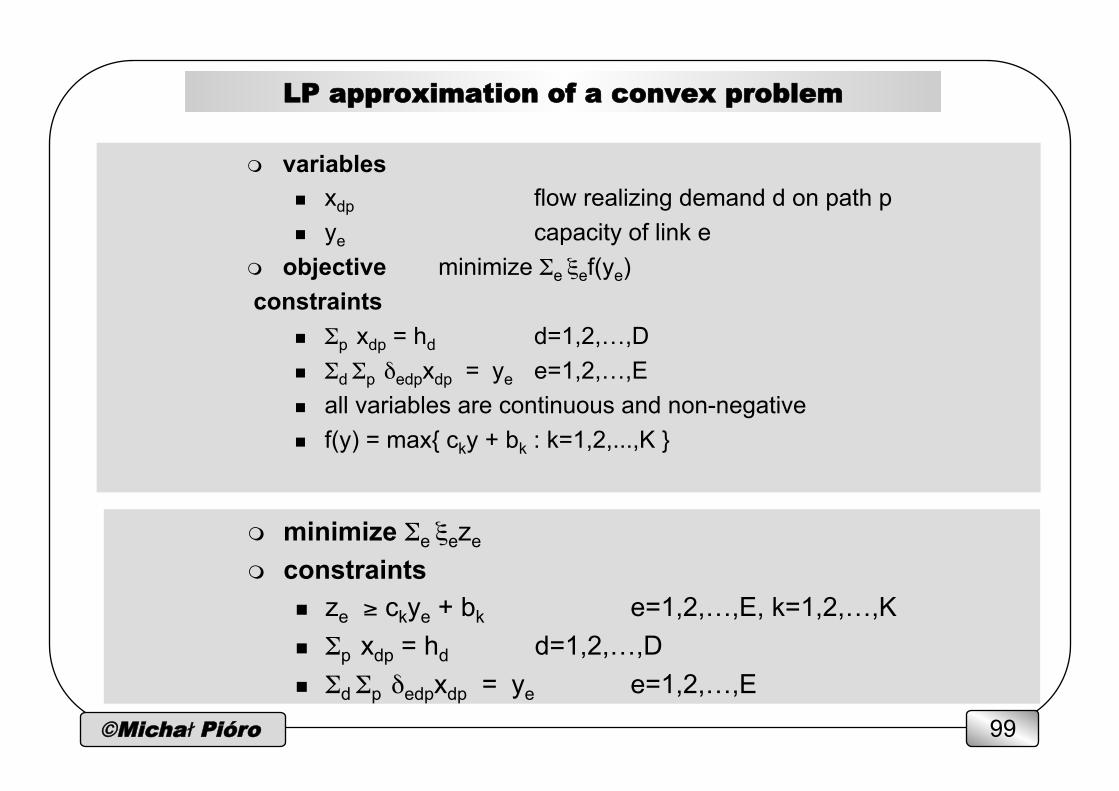
LP approximation of a convex problem
m minimize Σe ξeze m constraints
n ze ≥ ckye + bk e=1,2,…,E, k=1,2,…,K n Σp xdp = hd d=1,2,…,D n Σd Σp δedpxdp = ye e=1,2,…,E
m variables n xdp flow realizing demand d on path p n ye capacity of link e
m objective minimize Σe ξef(ye)
constraints n Σp xdp = hd d=1,2,…,D n Σd Σp δedpxdp = ye e=1,2,…,E n all variables are continuous and non-negative n f(y) = max{ cky + bk : k=1,2,...,K }
©Michał Pióro 100
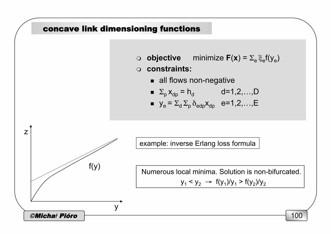
concave link dimensioning functions
f(y)
y
Numerous local minima. Solution is non-bifurcated. y1 < y2 → f(y1)/y1 > f(y2)/y2
m objective minimize F(x) = Σe ξef(ye) m constraints:
n all flows non-negative n Σp xdp = hd d=1,2,…,D n ye = Σd Σp δedpxdp e=1,2,…,E
z example: inverse Erlang loss formula
©Michał Pióro 101
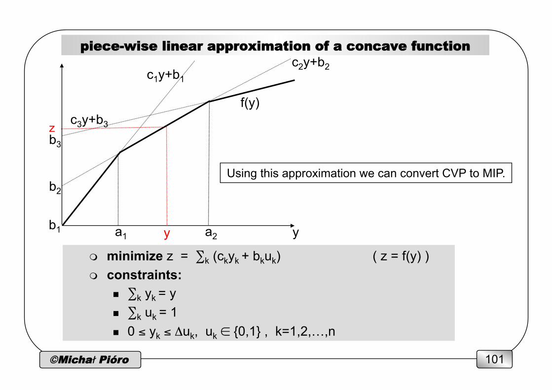
piece-wise linear approximation of a concave function
m minimize z = ∑k (ckyk + bkuk) ( z = f(y) ) m constraints:
n ∑k yk = y n ∑k uk = 1
n 0 ≤ yk ≤ Δuk, uk ∈ {0,1} , k=1,2,…,n
f(y)
y a1 a2
c3y+b3
c2y+b2 c1y+b1
b3
b2
y b1
Using this approximation we can convert CVP to MIP.
z
©Michał Pióro 102
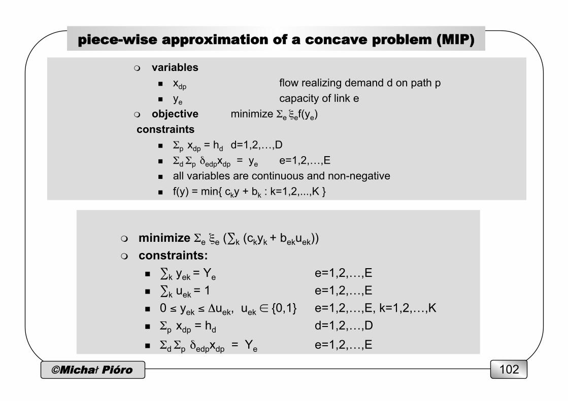
piece-wise approximation of a concave problem (MIP)
m minimize Σe ξe (∑k (ckyk + bekuek)) m constraints:
n ∑k yek = Ye e=1,2,…,E
n ∑k uek = 1 e=1,2,…,E
n 0 ≤ yek ≤ Δuek, uek ∈ {0,1} e=1,2,…,E, k=1,2,…,K n Σp xdp = hd d=1,2,…,D n Σd Σp δedpxdp = Ye e=1,2,…,E
m variables n xdp flow realizing demand d on path p n ye capacity of link e
m objective minimize Σe ξef(ye)
constraints n Σp xdp = hd d=1,2,…,D n Σd Σp δedpxdp = ye e=1,2,…,E n all variables are continuous and non-negative n f(y) = min{ cky + bk : k=1,2,...,K }
©Michał Pióro 103
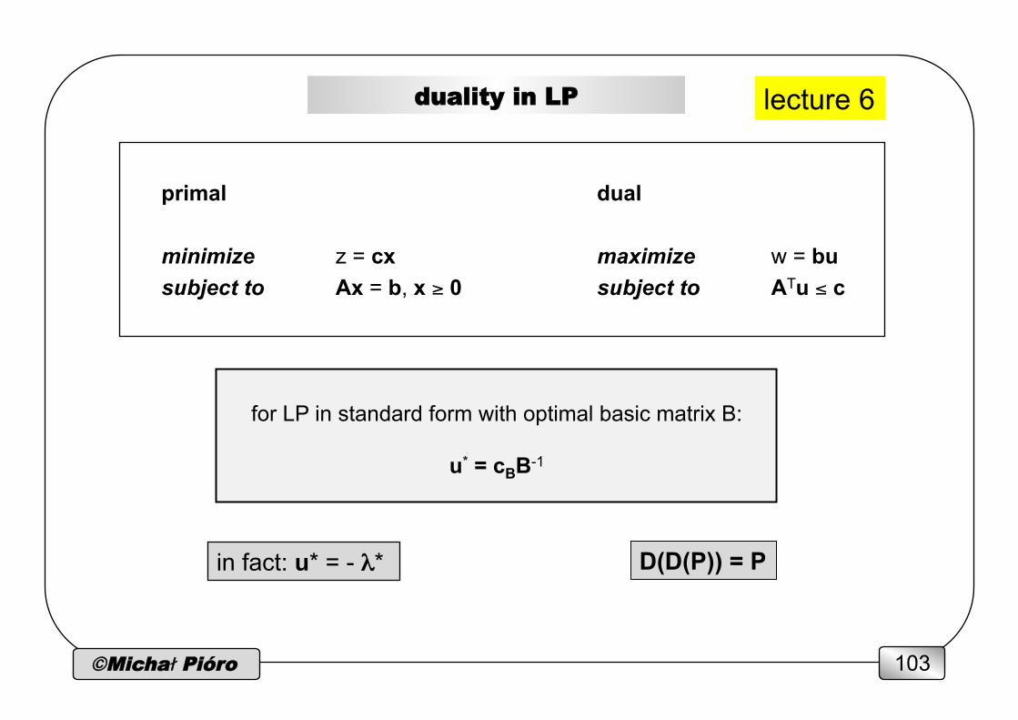
duality in LP
primal dual minimize z = cx maximize w = bu subject to Ax = b, x ≥ 0 subject to ATu ≤ c
for LP in standard form with optimal basic matrix B:
u* = cBB-1
in fact: u* = - λ* D(D(P)) = P
lecture 6
©Michał Pióro 104
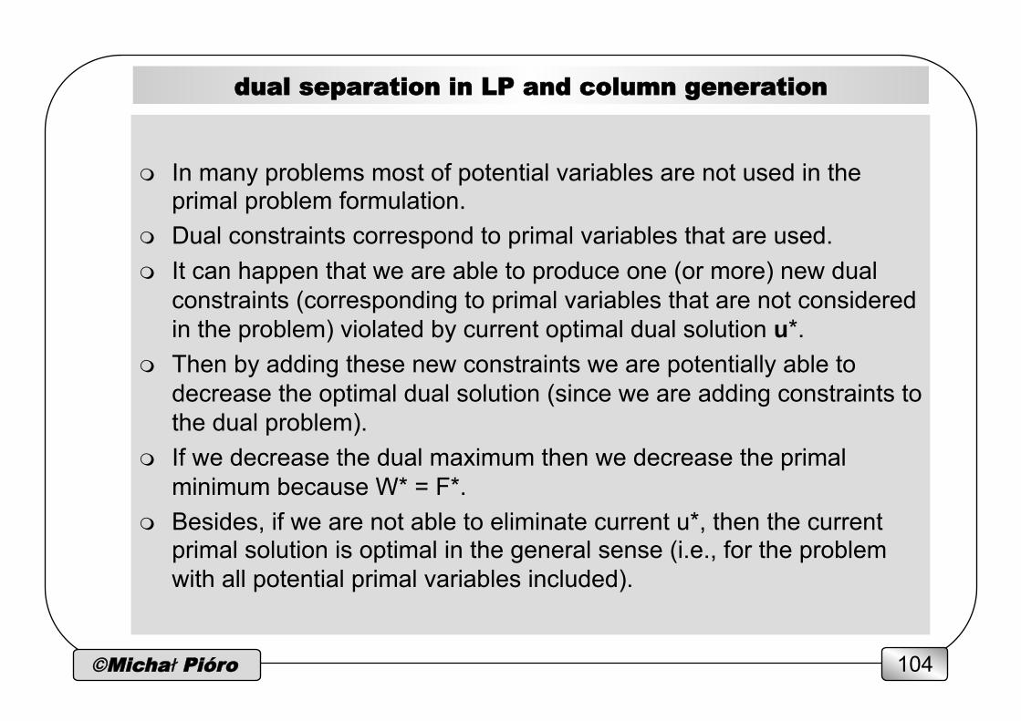
dual separation in LP and column generation
m In many problems most of potential variables are not used in the
primal problem formulation. m Dual constraints correspond to primal variables that are used. m It can happen that we are able to produce one (or more) new dual
constraints (corresponding to primal variables that are not considered in the problem) violated by current optimal dual solution u*.
m Then by adding these new constraints we are potentially able to decrease the optimal dual solution (since we are adding constraints to the dual problem).
m If we decrease the dual maximum then we decrease the primal minimum because W* = F*.
m Besides, if we are not able to eliminate current u*, then the current primal solution is optimal in the general sense (i.e., for the problem with all potential primal variables included).
©Michał Pióro 105
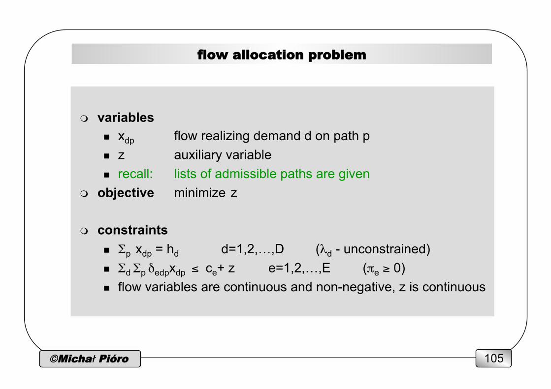
flow allocation problem
m variables n xdp flow realizing demand d on path p n z auxiliary variable n recall: lists of admissible paths are given
m objective minimize z
m constraints n Σp xdp = hd d=1,2,…,D (λd - unconstrained) n Σd Σp δedpxdp ≤ ce+ z e=1,2,…,E (πe ≥ 0) n flow variables are continuous and non-negative, z is continuous
©Michał Pióro 106
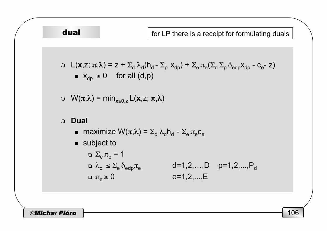
dual
m L(x,z; π,λ) = z + Σd λd(hd - Σp xdp) + Σe πe(Σd Σp δedpxdp - ce- z) n xdp ≥ 0 for all (d,p)
m W(π,λ) = minx≥0,z L(x,z; π,λ)
m Dual n maximize W(π,λ) = Σd λdhd - Σe πece n subject to
❏ Σe πe = 1 ❏ λd ≤ Σe δedpπe d=1,2,…,D p=1,2,...,Pd
❏ πe ≥ 0 e=1,2,...,E
for LP there is a receipt for formulating duals
©Michał Pióro 107
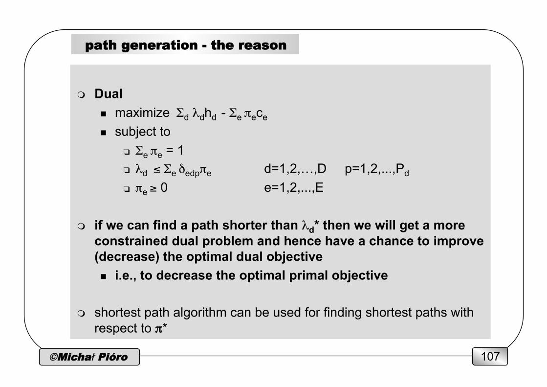
path generation - the reason
m Dual n maximize Σd λdhd - Σe πece n subject to
❏ Σe πe = 1 ❏ λd ≤ Σe δedpπe d=1,2,…,D p=1,2,...,Pd
❏ πe ≥ 0 e=1,2,...,E
m if we can find a path shorter than λd* then we will get a more constrained dual problem and hence have a chance to improve (decrease) the optimal dual objective n i.e., to decrease the optimal primal objective
m shortest path algorithm can be used for finding shortest paths with respect to π*
©Michał Pióro 108
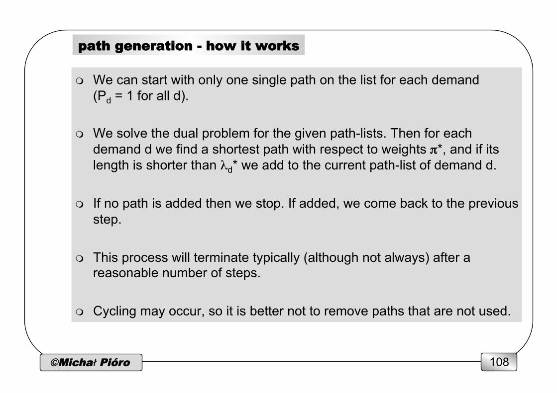
path generation - how it works
m We can start with only one single path on the list for each demand (Pd = 1 for all d).
m We solve the dual problem for the given path-lists. Then for each demand d we find a shortest path with respect to weights π*, and if its length is shorter than λd* we add to the current path-list of demand d.
m If no path is added then we stop. If added, we come back to the previous step.
m This process will terminate typically (although not always) after a reasonable number of steps.
m Cycling may occur, so it is better not to remove paths that are not used.
©Michał Pióro 109
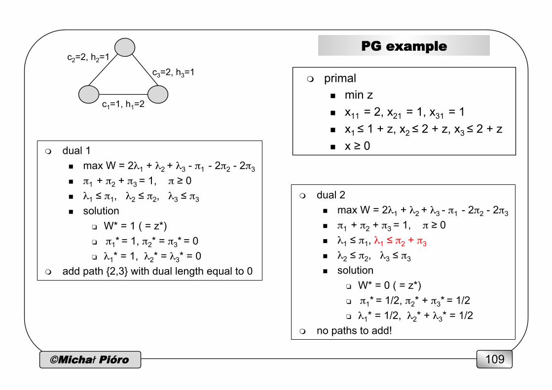
m primal n min z n x11 = 2, x21 = 1, x31 = 1
n x1 ≤ 1 + z, x2 ≤ 2 + z, x3 ≤ 2 + z
n x ≥ 0
PG example
c3=2, h3=1
c1=1, h1=2
c2=2, h2=1
m dual 1 n max W = 2λ1 + λ2 + λ3 - π1 - 2π2 - 2π3 n π1 + π2 + π3 = 1, π ≥ 0 n λ1 ≤ π1, λ2 ≤ π2, λ3 ≤ π3
n solution ❏ W* = 1 ( = z*)
❏ π1* = 1, π2* = π3* = 0 ❏ λ1* = 1, λ2* = λ3* = 0
m add path {2,3} with dual length equal to 0
m dual 2 n max W = 2λ1 + λ2 + λ3 - π1 - 2π2 - 2π3 n π1 + π2 + π3 = 1, π ≥ 0 n λ1 ≤ π1, λ1 ≤ π2 + π3 n λ2 ≤ π2, λ3 ≤ π3
n solution ❏ W* = 0 ( = z*)
❏ π1* = 1/2, π2* + π3* = 1/2 ❏ λ1* = 1/2, λ2* + λ3* = 1/2
m no paths to add!
©Michał Pióro 110
path generation
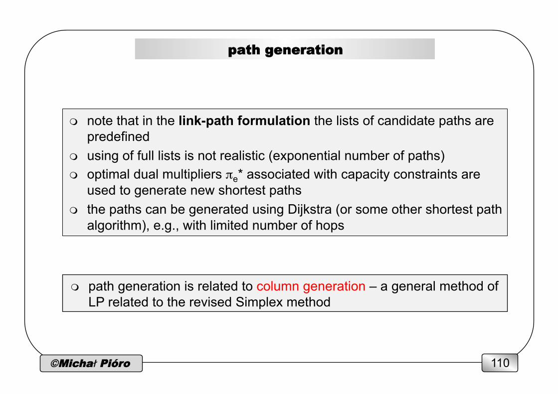
m note that in the link-path formulation the lists of candidate paths are predefined
m using of full lists is not realistic (exponential number of paths) m optimal dual multipliers πe* associated with capacity constraints are
used to generate new shortest paths m the paths can be generated using Dijkstra (or some other shortest path
algorithm), e.g., with limited number of hops
m path generation is related to column generation – a general method of LP related to the revised Simplex method
©Michał Pióro 111
optimization methods for MIP and IP
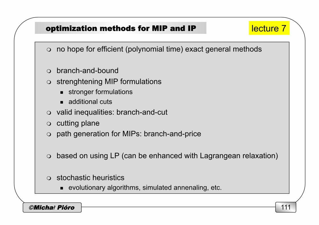
m no hope for efficient (polynomial time) exact general methods
m branch-and-bound m strenghtening MIP formulations
n stronger formulations n additional cuts
m valid inequalities: branch-and-cut m cutting plane m path generation for MIPs: branch-and-price
m based on using LP (can be enhanced with Lagrangean relaxation)
m stochastic heuristics n evolutionary algorithms, simulated annenaling, etc.
lecture 7

©Michał Pióro 112
strengthening MIP formulations: alternative formulations example: topological design (fixed charge link problem)
m variables n xdp flow of demand d on path p n ye capacity of link e n ue =1 if link e is installed; 0, otherwise
m objective minimize F = Σe ξeye + Σe κeue
m constraints
n Σp xdp = hd d=1,2,…,D n Σd Σp δedpxdp = ye e=1,2,…,E n ye ≤ Meue e=1,2,…,E n y and x non-negative, and u binary NP-hard
©Michał Pióro 113
Linear relaxation
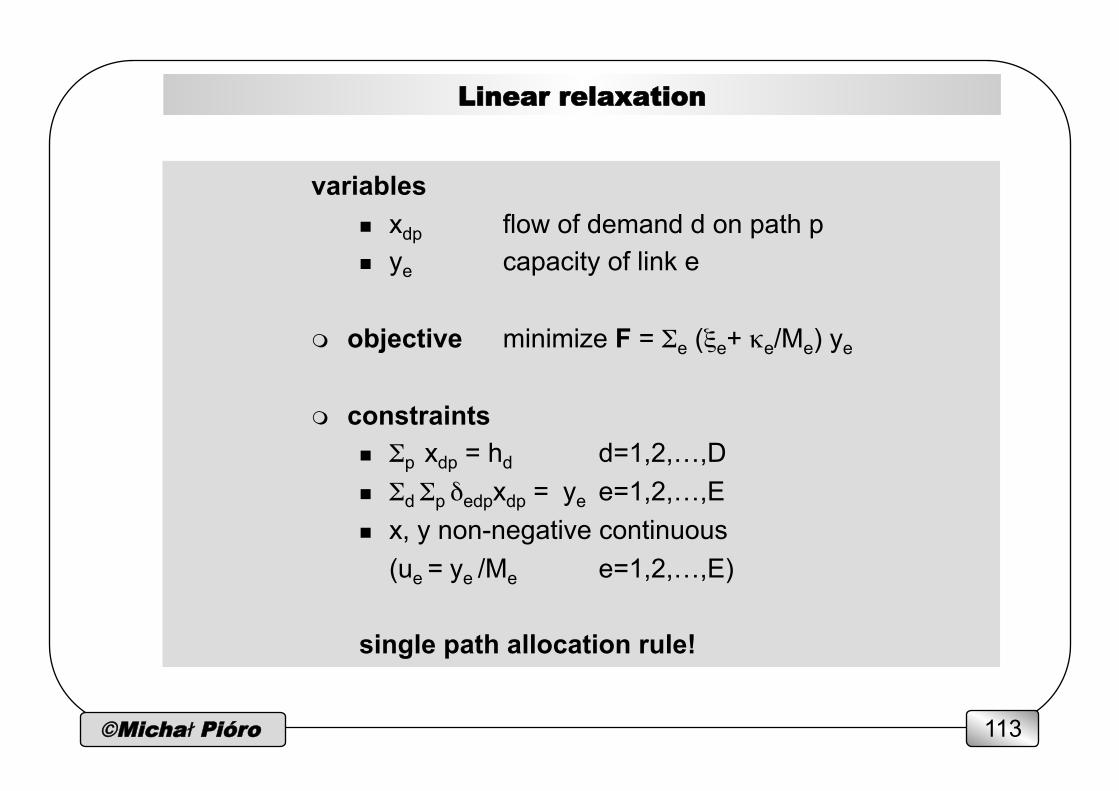
variables n xdp flow of demand d on path p n ye capacity of link e
m objective minimize F = Σe (ξe+ κe/Me) ye
m constraints
n Σp xdp = hd d=1,2,…,D n Σd Σp δedpxdp = ye e=1,2,…,E n x, y non-negative continuous
(ue = ye /Me e=1,2,…,E) single path allocation rule!

©Michał Pióro 114
B&B subproblem: Linear relaxation LR(NU,N0,N1)
variables n xdp flow of demand d on path p n ye capacity of link e n ue link status variable
m objective minimize F = Σe (ξeye + κeue)
m constraints
n Σp xdp = hd d=1,2,…,D n Σd Σp δedpxdp = ye e=1,2,…,E n ye ≤ Meue e=1,2,…,E n 0 ≤ ue ≤ 1 e ∈ NU n ue = 0 for e ∈ N0, ue = 1 for e ∈ N1
n x, y non-negative continuous
©Michał Pióro 115
Lower bounds I
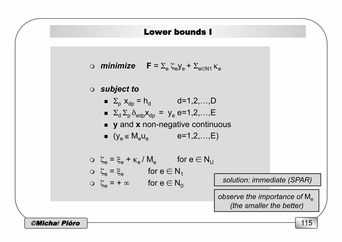
m minimize F = Σe ζeye + Σe∈N1 κe
m subject to
n Σp xdp = hd d=1,2,…,D n Σd Σp δedpxdp = ye e=1,2,…,E n y and x non-negative continuous n (ye ≤ Meue e=1,2,…,E)
m ζe = ξe + κe / Me for e ∈ NU m ζe = ξe for e ∈ N1
m ζe = + ∞ for e ∈ N0
observe the importance of Me (the smaller the better)
solution: immediate (SPAR)
©Michał Pióro 116
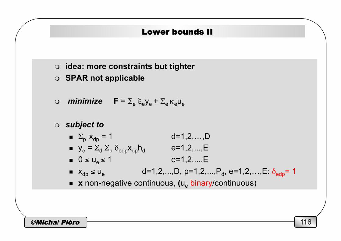
Lower bounds II
m idea: more constraints but tighter m SPAR not applicable
m minimize F = Σe ξeye + Σe κeue
m subject to
n Σp xdp = 1 d=1,2,…,D n ye = Σd Σp δedpxdphd e=1,2,...,E n 0 ≤ ue ≤ 1 e=1,2,...,E n xdp ≤ ue d=1,2,...,D, p=1,2,...,Pd, e=1,2,…,E: δedp= 1 n x non-negative continuous, (ue binary/continuous)

©Michał Pióro 117
Lower bounds II – B&B subproblems
m minimize F = Σe ξeye + Σe κeue
m subject to
n Σp xdp = 1 d=1,2,…,D n ye = Σd Σp δedpxdphd e=1,2,...,E n 0 ≤ ue ≤ 1 e ∈ NU n ue = 0 e ∈ N0
n ue = 1 e ∈ N1 n xdp ≤ ue d=1,2,...,D, p=1,2,...,Pd, e=1,2,…,E: δedp= 1 n x non-negative continuous, (ue: e ∈ NU) continuous
©Michał Pióro 118
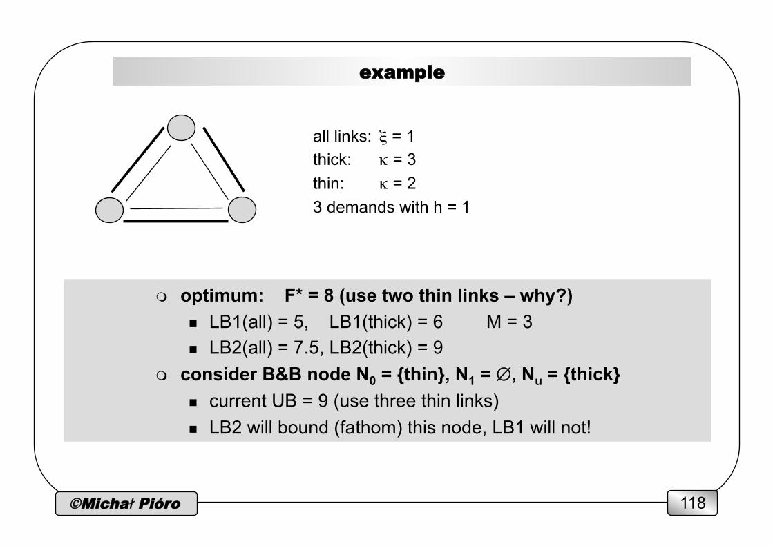
example
m optimum: F* = 8 (use two thin links – why?) n LB1(all) = 5, LB1(thick) = 6 M = 3 n LB2(all) = 7.5, LB2(thick) = 9
m consider B&B node N0 = {thin}, N1 = ∅, Nu = {thick} n current UB = 9 (use three thin links) n LB2 will bound (fathom) this node, LB1 will not!
all links: ξ = 1 thick: κ = 3 thin: κ = 2 3 demands with h = 1
©Michał Pióro 119
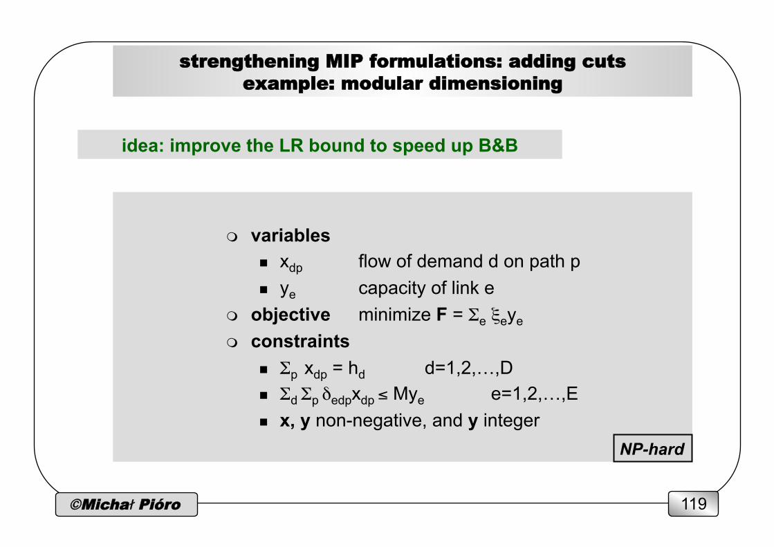
strengthening MIP formulations: adding cuts example: modular dimensioning
m variables n xdp flow of demand d on path p n ye capacity of link e
m objective minimize F = Σe ξeye
m constraints n Σp xdp = hd d=1,2,…,D n Σd Σp δedpxdp ≤ Mye e=1,2,…,E n x, y non-negative, and y integer
idea: improve the LR bound to speed up B&B
NP-hard
©Michał Pióro 120
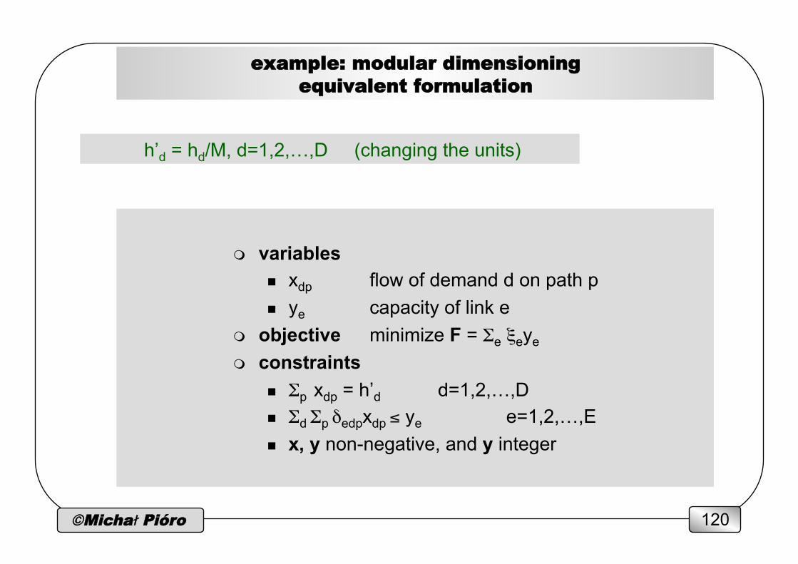
example: modular dimensioning equivalent formulation
m variables n xdp flow of demand d on path p n ye capacity of link e
m objective minimize F = Σe ξeye
m constraints n Σp xdp = h’d d=1,2,…,D n Σd Σp δedpxdp ≤ ye e=1,2,…,E n x, y non-negative, and y integer
h’d = hd/M, d=1,2,…,D (changing the units)

©Michał Pióro 121
example: modular dimensioning
m valid inequality n Σ e∈E(V1,V2) ye ≥ ⎡Σ d∈D(V1,V2) h’d⎤ equivalent formulationn Σ e∈E(V1,V2) ye ≥ ⎡Σ d∈D(V1,V2) hd/M⎤ original formulation
❏ (V1,V2) – cut in the network graph, V1 ∪ V2 = V, V1 ∩ V2 = ∅, V1, V2 ≠ ∅
m for example: generate such inequalities for all nodes and pairs of nodes
V1 V2
©Michał Pióro 122
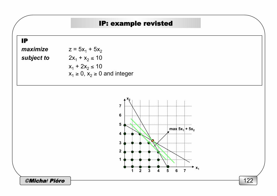
IP: example revisted
IP maximize z = 5x1 + 5x2 subject to 2x1 + x2 ≤ 10
x1 + 2x2 ≤ 10 x1 ≥ 0, x2 ≥ 0 and integer
7
6
5
4
3
2
1
6 7 5 4 3 2 1
max 5x1 + 5x2
x2
x1

©Michał Pióro 123
conv(XIP)
IP maximize z = 5x1 + 5x2 subject to 2x1 + x2 ≤ 10
x1 + 2x2 ≤ 10 x1 + x2 ≤ 6 (cut) x1 ≥ 0, x2 ≥ 0 and integer
7
6
5
4
3
2
1
6 7 5 4 3 2 1
x2
x1
©Michał Pióro 124
cutting plane method for IP (Gomory)
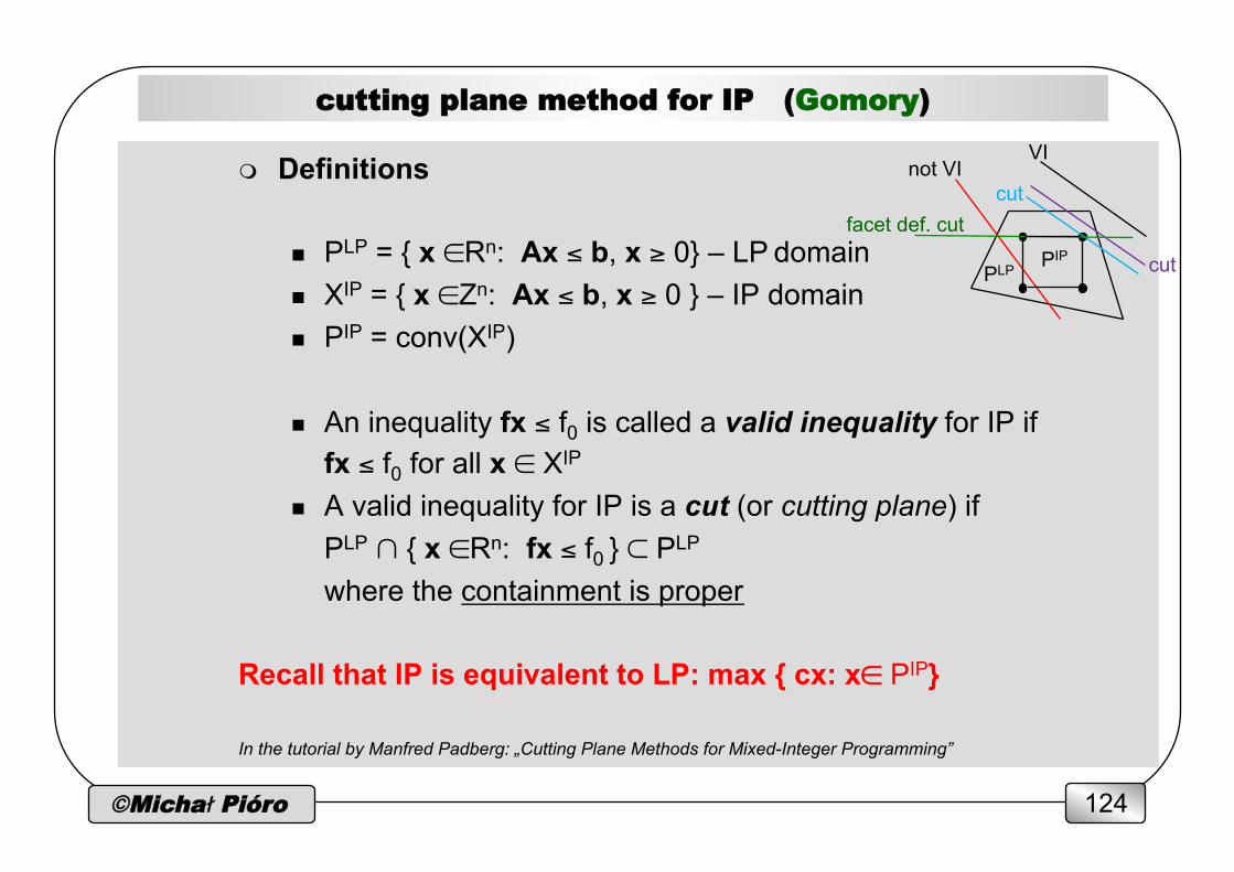
m Definitions
n PLP = { x ∈Rn: Ax ≤ b, x ≥ 0} – LP domain n XIP = { x ∈Zn: Ax ≤ b, x ≥ 0 } – IP domain n PIP = conv(XIP)
n An inequality fx ≤ f0 is called a valid inequality for IP if fx ≤ f0 for all x ∈ XIP
n A valid inequality for IP is a cut (or cutting plane) if PLP ∩ { x ∈Rn: fx ≤ f0 } ⊂ PLP where the containment is proper
Recall that IP is equivalent to LP: max { cx: x∈ PIP} In the tutorial by Manfred Padberg: „Cutting Plane Methods for Mixed-Integer Programming”
VI
cut
cut not VI
facet def. cut
PIP PLP
©Michał Pióro 125
cutting plane method - continued
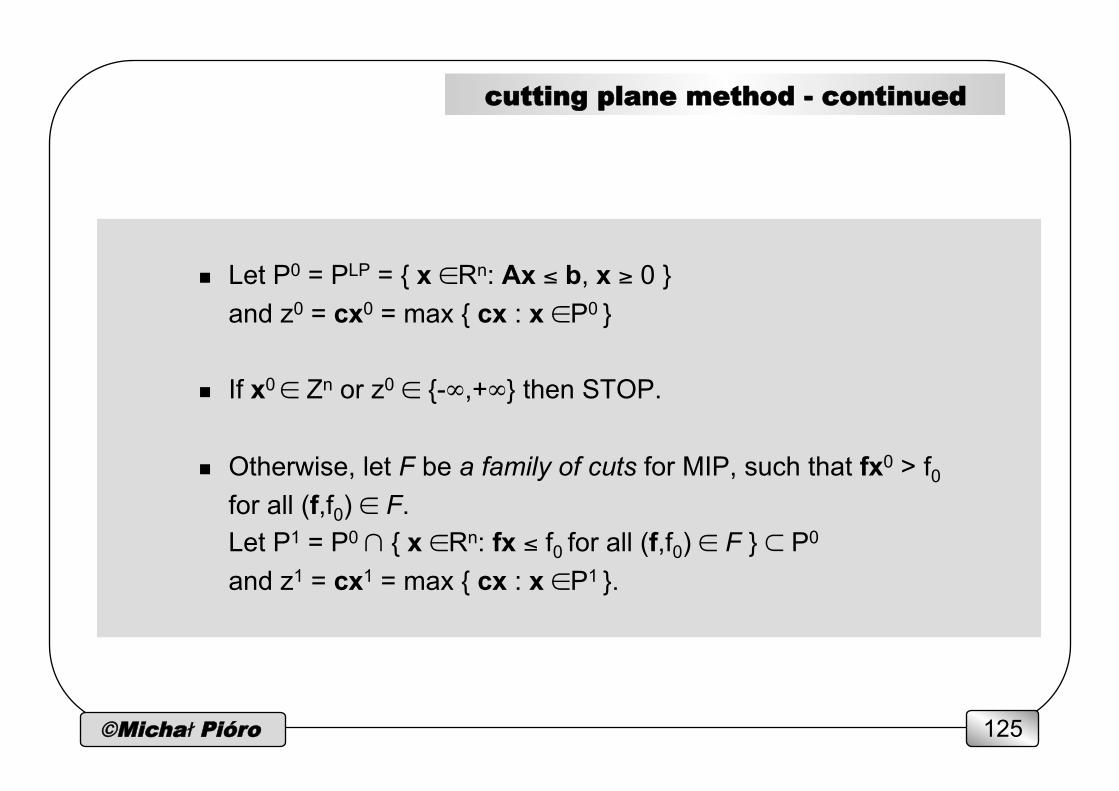
n Let P0 = PLP = { x ∈Rn: Ax ≤ b, x ≥ 0 } and z0 = cx0 = max { cx : x ∈P0 }
n If x0 ∈ Zn or z0 ∈ {-∞,+∞} then STOP.
n Otherwise, let F be a family of cuts for MIP, such that fx0 > f0 for all (f,f0) ∈ F. Let P1 = P0 ∩ { x ∈Rn: fx ≤ f0 for all (f,f0) ∈ F } ⊂ P0
and z1 = cx1 = max { cx : x ∈P1 }.

©Michał Pióro 126
cutting plane method - continued
n Note that XIP ⊆ P1 ⊂ P0 and we can iterate, generating a sequence of polyhedra P0 ⊃ P1 ⊃ ... ⊃ Pk ⊃ Pk+1 ⊃ ... ⊆ conv(XIP) ⊆ XIP such that zk+1 = cxk+1 ≤ zk = cxk where zk = cxk = max { cx : x ∈Pk }.
n We stop when xk ∈ Zn or zk = -∞ (i.e., when Pk = ∅).

©Michał Pióro 127
Gomory cutting plane method – details for IP
Wolsey – Integer Programming
Integer Program (IP)
maximize z = cx (zIP) subject to Ax = b, x ≥ 0 (linear constraints)
x integer (integrality constraint)
Assumption: A, b – integer Idea n solve the associated LP relaxation n find optimal basis n choose a basic variable that is not integer n generate a Chvátal-Gomory inequality using the constraint associated with this basic variable to cut-off the current relaxed solution
©Michał Pióro 128
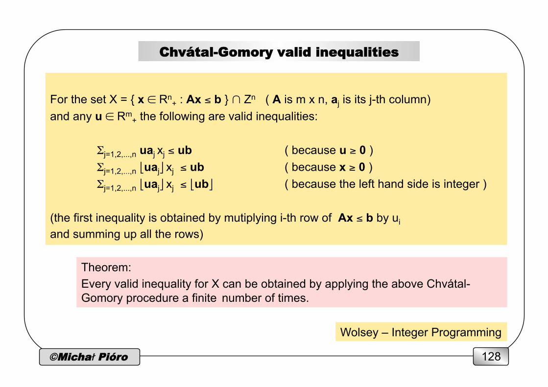
Chvátal-Gomory valid inequalities
For the set X = { x ∈ Rn+ : Ax ≤ b } ∩ Zn ( A is m x n, aj is its j-th column)
and any u ∈ Rm+ the following are valid inequalities:
Σj=1,2,...,n uaj xj ≤ ub ( because u ≥ 0 ) Σj=1,2,...,n ⎣uaj⎦ xj ≤ ub ( because x ≥ 0 ) Σj=1,2,...,n ⎣uaj⎦ xj ≤ ⎣ub⎦ ( because the left hand side is integer )
(the first inequality is obtained by mutiplying i-th row of Ax ≤ b by ui and summing up all the rows)
Theorem: Every valid inequality for X can be obtained by applying the above Chvátal- Gomory procedure a finite number of times.
Wolsey – Integer Programming
©Michał Pióro 129
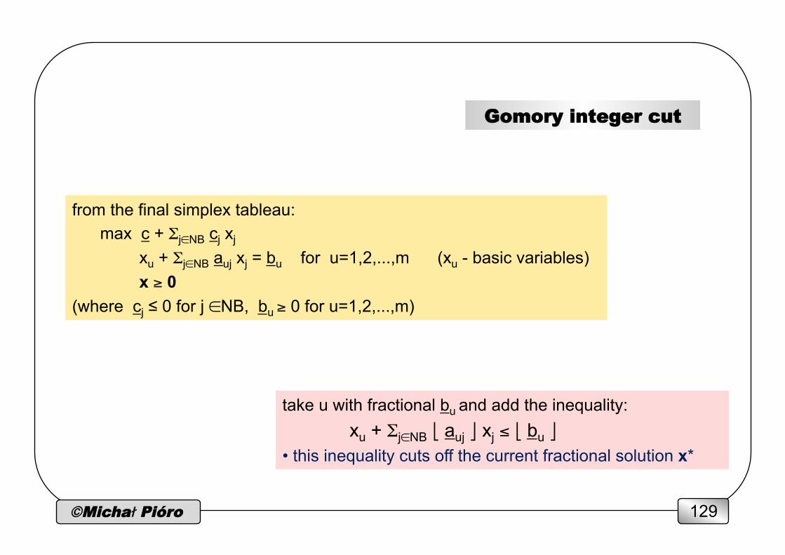
Gomory integer cut
from the final simplex tableau: max c + Σj∈NB cj xj
xu + Σj∈NB auj xj = bu for u=1,2,...,m (xu - basic variables) x ≥ 0
(where cj ≤ 0 for j ∈NB, bu ≥ 0 for u=1,2,...,m)
take u with fractional bu and add the inequality: xu + Σj∈NB ⎣ auj ⎦ xj ≤ ⎣ bu ⎦
• this inequality cuts off the current fractional solution x*
©Michał Pióro 130
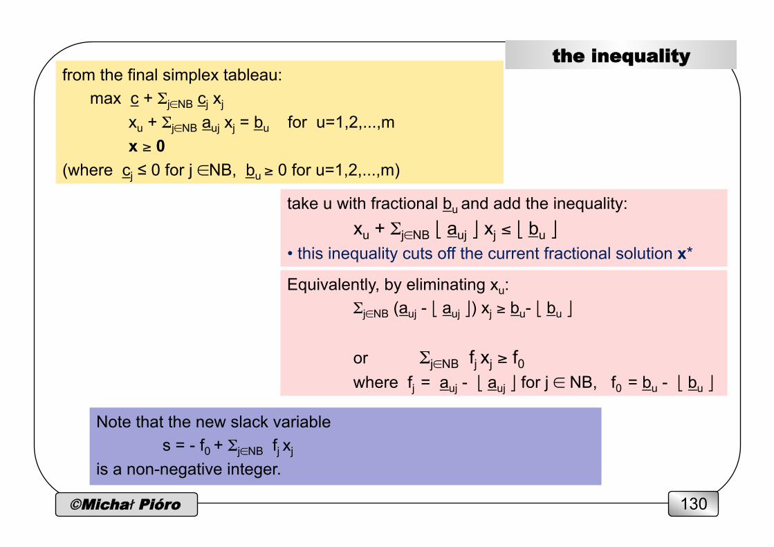
the inequality from the final simplex tableau: max c + Σj∈NB cj xj
xu + Σj∈NB auj xj = bu for u=1,2,...,m x ≥ 0
(where cj ≤ 0 for j ∈NB, bu ≥ 0 for u=1,2,...,m)
take u with fractional bu and add the inequality: xu + Σj∈NB ⎣ auj ⎦ xj ≤ ⎣ bu ⎦
• this inequality cuts off the current fractional solution x*
Note that the new slack variable s = - f0 + Σj∈NB fj xj
is a non-negative integer.
Equivalently, by eliminating xu: Σj∈NB (auj - ⎣ auj ⎦) xj ≥ bu- ⎣ bu ⎦
or Σj∈NB fj xj ≥ f0 where fj = auj - ⎣ auj ⎦ for j ∈ NB, f0 = bu - ⎣ bu ⎦

©Michał Pióro 131
cutting plane method - discussion
m Is it always possible to find a cut that cuts off the LP optimum?
n YES – the previous method.
m Does there exist a cut generation mechanism which guarantees the finite number of steps?
n NO, only for IP (certainly, the number of iterations is in general exponential).
n For general mixed integer programs this is an open question. n For MIPs finite converge is guaranteed if the objective function is integer valued.
©Michał Pióro 132
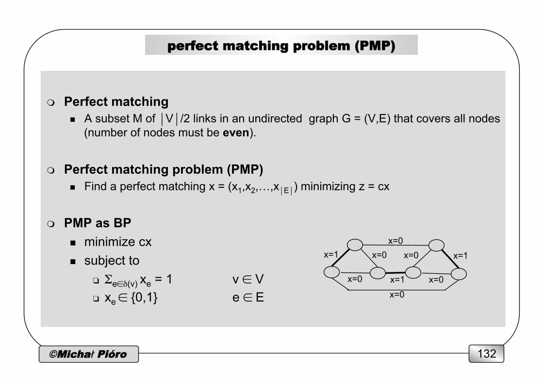
perfect matching problem (PMP)
m Perfect matching n A subset M of ⏐V⏐/2 links in an undirected graph G = (V,E) that covers all nodes
(number of nodes must be even).
m Perfect matching problem (PMP) n Find a perfect matching x = (x1,x2,…,x⏐E⏐) minimizing z = cx
m PMP as BP n minimize cx n subject to
❏ Σe∈δ(v) xe = 1 v ∈ V ❏ xe ∈ {0,1} e ∈ E
x=1
x=0
x=0 x=0
x=0
x=1
x=0 x=1
x=0
©Michał Pióro 133
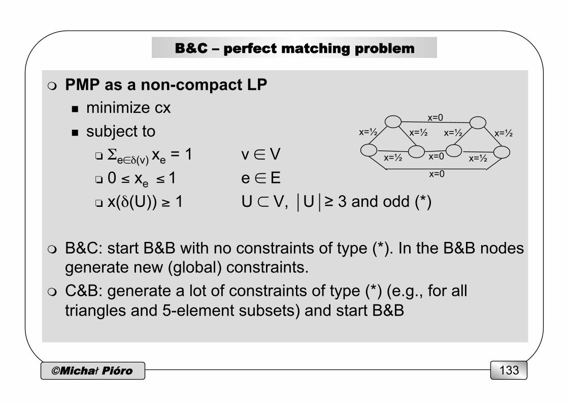
B&C – perfect matching problem
m PMP as a non-compact LP n minimize cx n subject to
❏ Σe∈δ(v) xe = 1 v ∈ V ❏ 0 ≤ xe ≤ 1 e ∈ E ❏ x(δ(U)) ≥ 1 U ⊂ V, ⏐U⏐≥ 3 and odd (*)
m B&C: start B&B with no constraints of type (*). In the B&B nodes generate new (global) constraints.
m C&B: generate a lot of constraints of type (*) (e.g., for all triangles and 5-element subsets) and start B&B
x=½
x=½
x=½ x=½
x=½
x=½
x=0
x=0
x=0
©Michał Pióro 134
B&B algorithim - comments
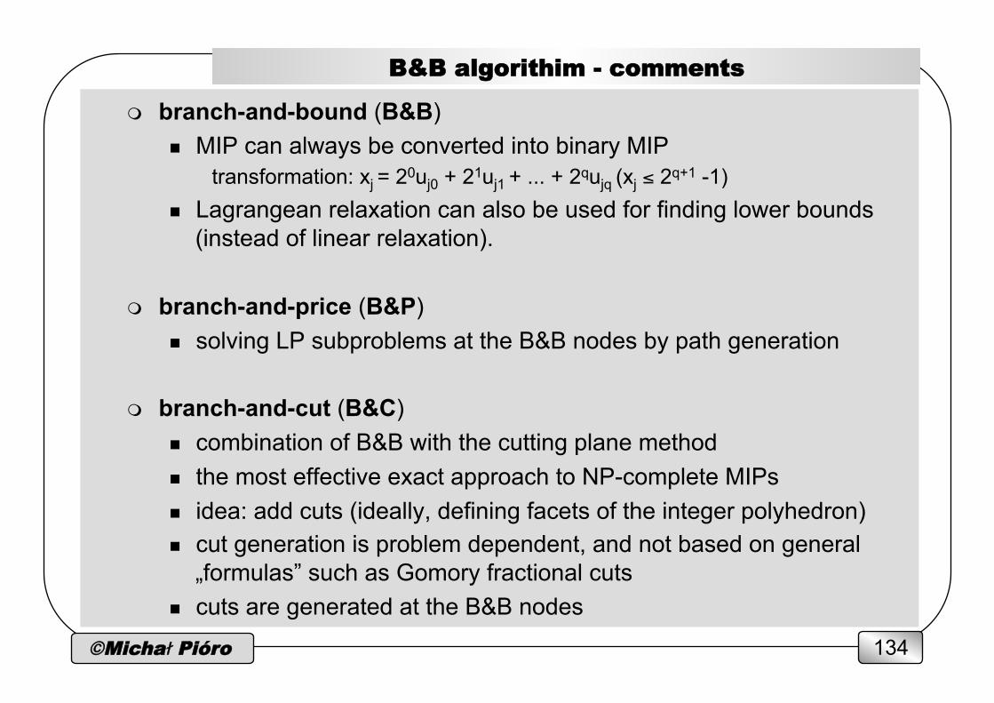
m branch-and-bound (B&B) n MIP can always be converted into binary MIP
transformation: xj = 20uj0 + 21uj1 + ... + 2qujq (xj ≤ 2q+1 -1) n Lagrangean relaxation can also be used for finding lower bounds
(instead of linear relaxation).
m branch-and-price (B&P) n solving LP subproblems at the B&B nodes by path generation
m branch-and-cut (B&C)
n combination of B&B with the cutting plane method n the most effective exact approach to NP-complete MIPs n idea: add cuts (ideally, defining facets of the integer polyhedron) n cut generation is problem dependent, and not based on general
„formulas” such as Gomory fractional cuts n cuts are generated at the B&B nodes

©Michał Pióro 135
wireless mesh network (WMN) design lecture 8
m WMN provide inexpensive broadband access to the Internet
m deployed by communities/authorities/companies in metropolitan and residential areas
m based on wireless networking standards n IEEE 802.11 family (Wi-Fi) n IEEE 806.16 family (WiMAX) n IEEE 802.15.5 (bluetooth, home applications)
m using off-the-shelf wireless communication components and technologies
m specific features of radio communications and the data link layer protocols make optimization difficult

©Michał Pióro 136
broadband Internet access via WMN
©Michał Pióro 137
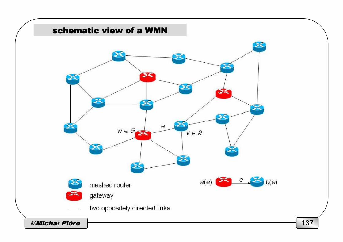
schematic view of a WMN
©Michał Pióro 138
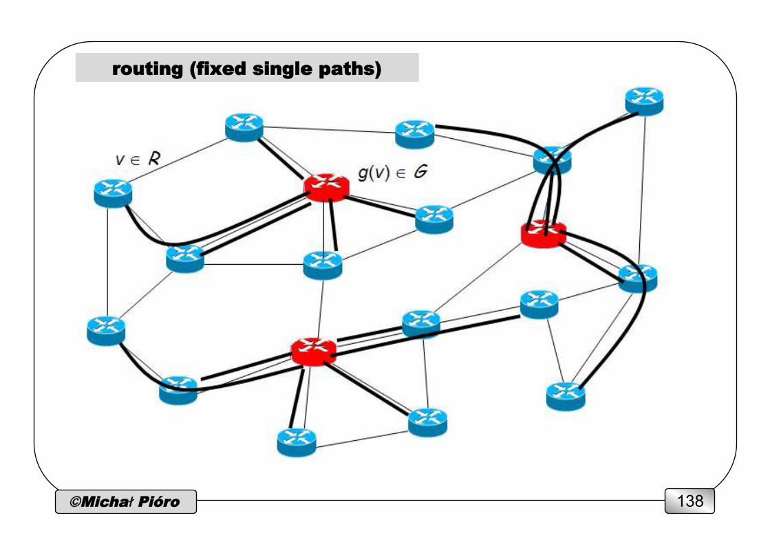
routing (fixed single paths)
©Michał Pióro 139
transmission scheduling (TDMA)
t=T t=2 t=1 …
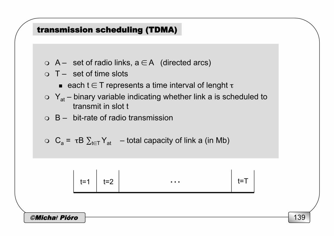
m A – set of radio links, a ∈ A (directed arcs) m T – set of time slots
n each t ∈ T represents a time interval of lenght τ m Yat – binary variable indicating whether link a is scheduled to
transmit in slot t m B – bit-rate of radio transmission
m Ca = τB ∑t∈T Yat – total capacity of link a (in Mb)
©Michał Pióro 140
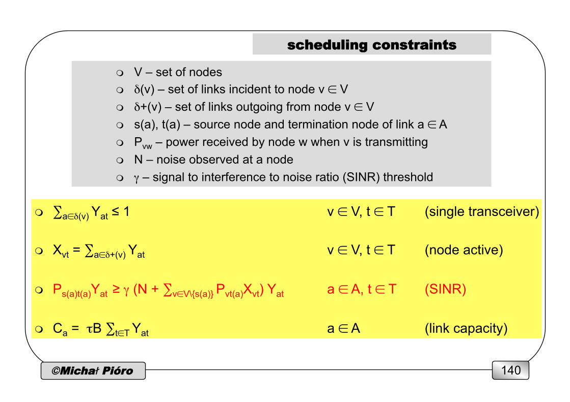
scheduling constraints
m V – set of nodes m δ(v) – set of links incident to node v ∈ V m δ+(v) – set of links outgoing from node v ∈ V m s(a), t(a) – source node and termination node of link a ∈ A m Pvw – power received by node w when v is transmitting m N – noise observed at a node m γ – signal to interference to noise ratio (SINR) threshold
m ∑a∈δ(v) Yat ≤ 1 v ∈ V, t ∈ T (single transceiver) m Xvt = ∑a∈δ+(v) Yat v ∈ V, t ∈ T (node active) m Ps(a)t(a)Yat ≥ γ (N + ∑v∈V\{s(a)} Pvt(a)Xvt) Yat a ∈ A, t ∈ T (SINR) m Ca = τB ∑t∈T Yat a ∈ A (link capacity)

©Michał Pióro 141
max-min flow problem
m V – set nodes, V = G ∪ R n G – set of gateways n R – set of mesh routers
m g(r) – the gateway selected for mesh router r ∈ R m R(r) – fixed route (path) from g(r) ∈ G down to r, for each r ∈ R m n(a) – number of routes using link a ∈ A m f – total downloaded data volume for each mesh router (elastic traffic)
m maximize f n n(a)f ≤ Ca a ∈ A n plus the scheduling constraints
NP-hard, this formulation is in fact intractable.
©Michał Pióro 142
compatible sets
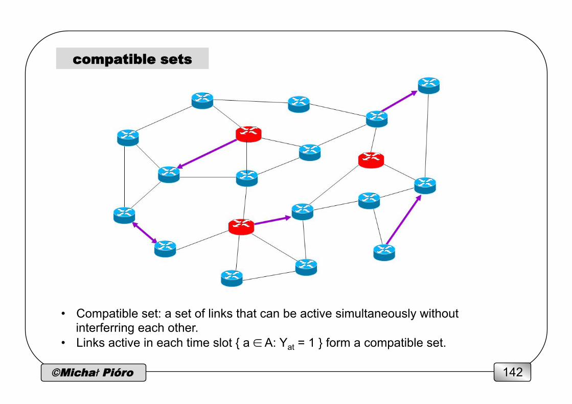
• Compatible set: a set of links that can be active simultaneously without interferring each other.
• Links active in each time slot { a ∈ A: Yat = 1 } form a compatible set.
©Michał Pióro 143
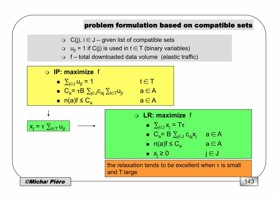
m C(j), i ∈ J – given list of compatible sets m ujt = 1 if C(j) is used in t ∈ T (binary variables) m f – total downloaded data volume (elastic traffic)
m IP: maximize f n ∑j∈J ujt = 1 t ∈ T n Ca= τB ∑j∈Jcaj ∑t∈Tujt a ∈ A n n(a)f ≤ Ca a ∈ A
problem formulation based on compatible sets
m LR: maximize f n ∑j∈J xj = Tτ n Ca= B ∑j∈J cajxj a ∈ A n n(a)f ≤ Ca a ∈ A n xj ≥ 0 j ∈ J
xj = τ ∑t∈T ujt
the relaxation tends to be excellent when τ is small and T large
©Michał Pióro 144
generating compatible sets
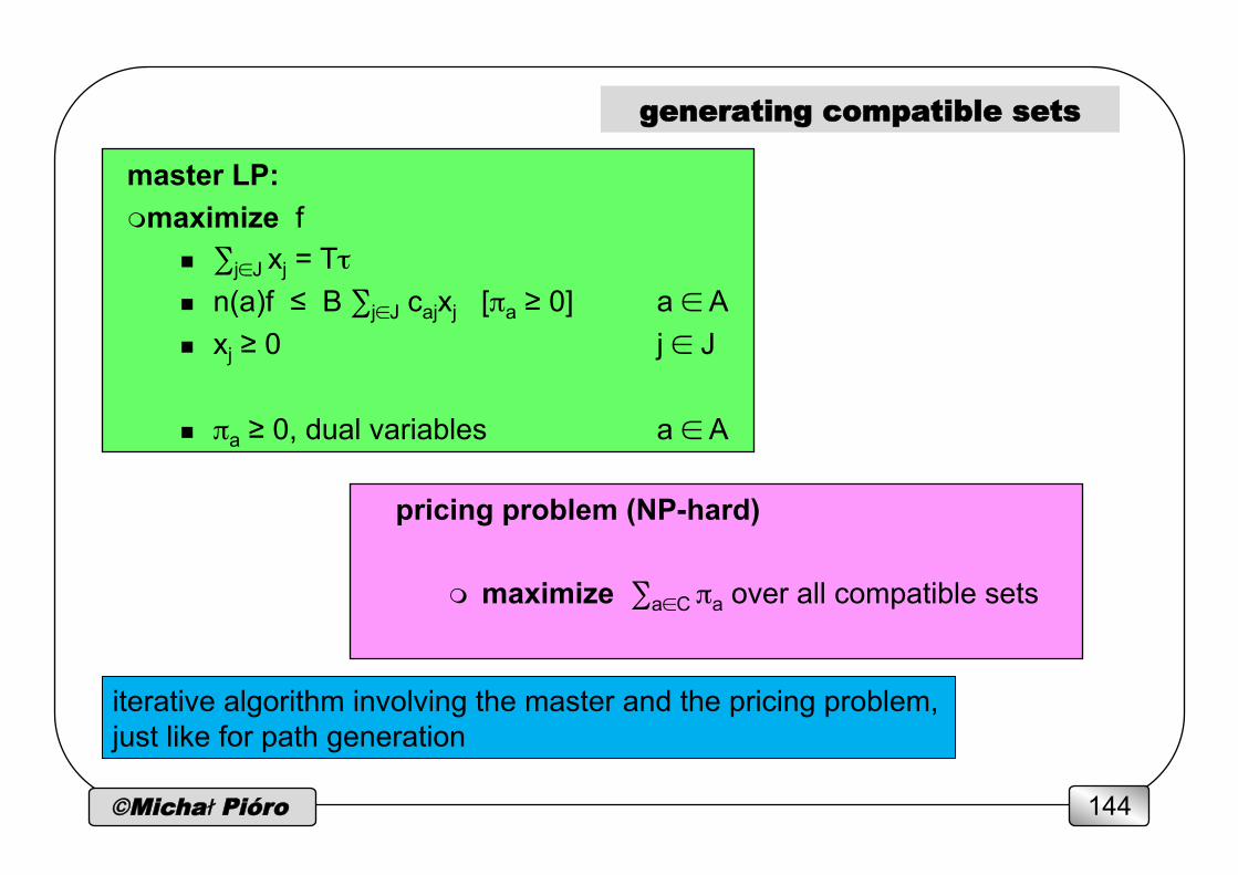
master LP: m maximize f
n ∑j∈J xj = Tτ n n(a)f ≤ B ∑j∈J cajxj [πa ≥ 0] a ∈ A n xj ≥ 0 j ∈ J
n πa ≥ 0, dual variables a ∈ A
pricing problem (NP-hard)
m maximize ∑a∈C πa over all compatible sets
iterative algorithm involving the master and the pricing problem, just like for path generation
©Michał Pióro 145
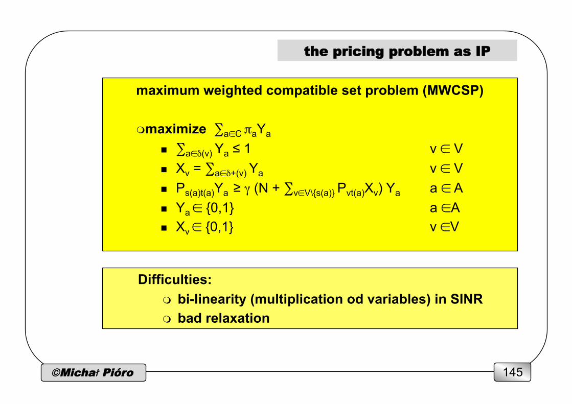
the pricing problem as IP
maximum weighted compatible set problem (MWCSP)
m maximize ∑a∈C πaYa
n ∑a∈δ(v) Ya ≤ 1 v ∈ V n Xv = ∑a∈δ+(v) Ya v ∈ V n Ps(a)t(a)Ya ≥ γ (N + ∑v∈V\{s(a)} Pvt(a)Xv) Ya a ∈ A n Ya ∈ {0,1} a ∈A n Xv ∈ {0,1} v ∈V
Difficulties: m bi-linearity (multiplication od variables) in SINR m bad relaxation
©Michał Pióro 146
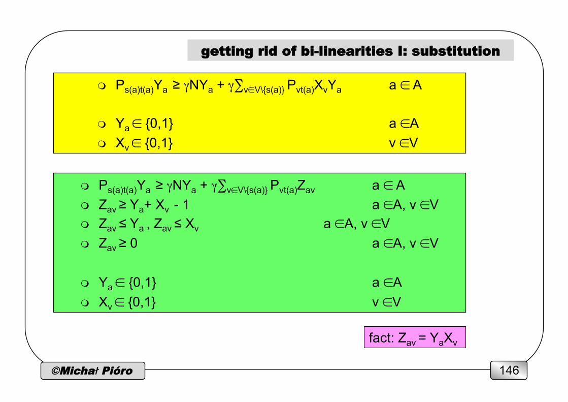
getting rid of bi-linearities I: substitution
m Ps(a)t(a)Ya ≥ γNYa + γ∑v∈V\{s(a)} Pvt(a)XvYa a ∈ A
m Ya ∈ {0,1} a ∈A m Xv ∈ {0,1} v ∈V
m Ps(a)t(a)Ya ≥ γNYa + γ∑v∈V\{s(a)} Pvt(a)Zav a ∈ A m Zav ≥ Ya+ Xv - 1 a ∈A, v ∈V m Zav ≤ Ya , Zav ≤ Xv a ∈A, v ∈V m Zav ≥ 0 a ∈A, v ∈V
m Ya ∈ {0,1} a ∈A m Xv ∈ {0,1} v ∈V
fact: Zav = YaXv
©Michał Pióro 147
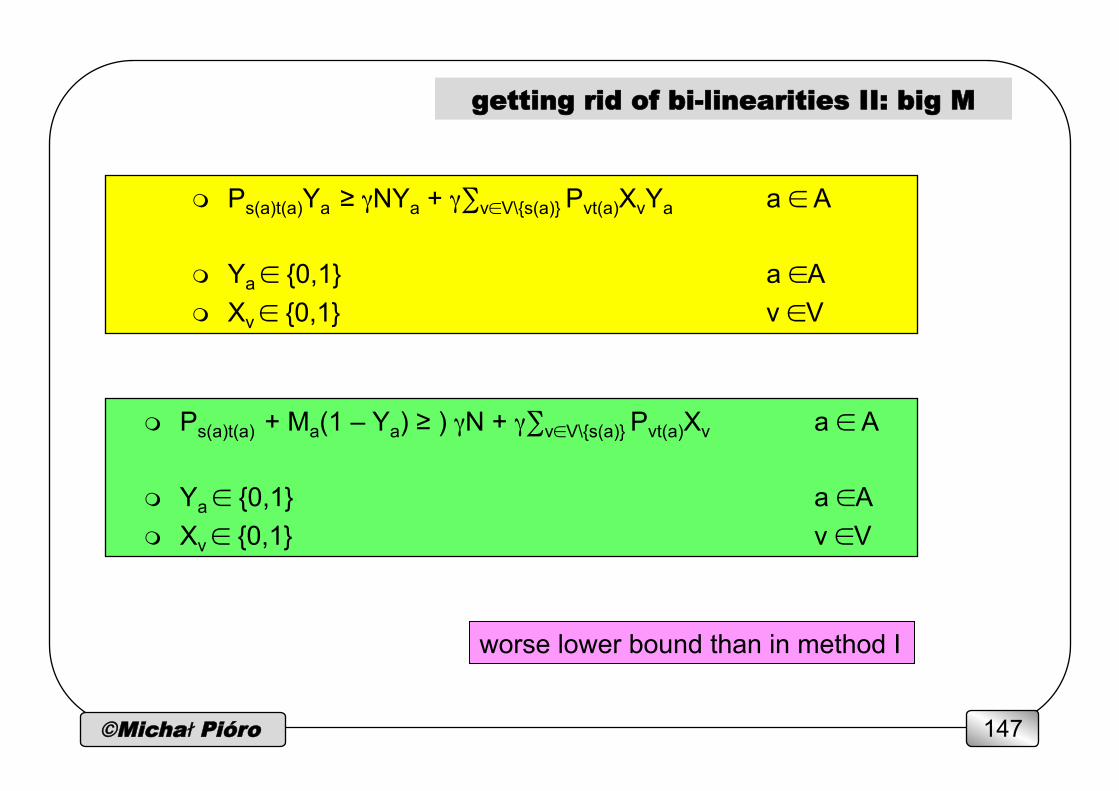
getting rid of bi-linearities II: big M
m Ps(a)t(a)Ya ≥ γNYa + γ∑v∈V\{s(a)} Pvt(a)XvYa a ∈ A
m Ya ∈ {0,1} a ∈A m Xv ∈ {0,1} v ∈V
m Ps(a)t(a) + Ma(1 – Ya) ≥ ) γN + γ∑v∈V\{s(a)} Pvt(a)Xv a ∈ A
m Ya ∈ {0,1} a ∈A m Xv ∈ {0,1} v ∈V
worse lower bound than in method I

©Michał Pióro 148
m undirected graph (V,E) corresponding to the bidirected graph (V,A) m x = (xe, e ∈ E) – a given vector of binary edge variables m matching: a subset of edges S(x) = {e ∈ E: xe = 1 } when ⏐Σe∈δ(v)
xe ⏐≤ 1 for all v ∈ V m matching polytope (vertices = matchings)
n x(δ(v)) ≤ 1 v ∈ V n ⏐x(E[U])⏐≤ (⏐U⏐-1)/2 U ∈ O(V) n xe ≥ 0 e ∈ E
n where ❏ E[U] set of all edges with both ends in U ❏ O(V) family of all odd subsets of V ❏ x(W) = Σe∈W xe for W ⊆ E
x=1
x=0
x=0 x=0
x=0
x=1
x=0 x=1
x=0
valid inequalities: matching
©Michał Pióro 149
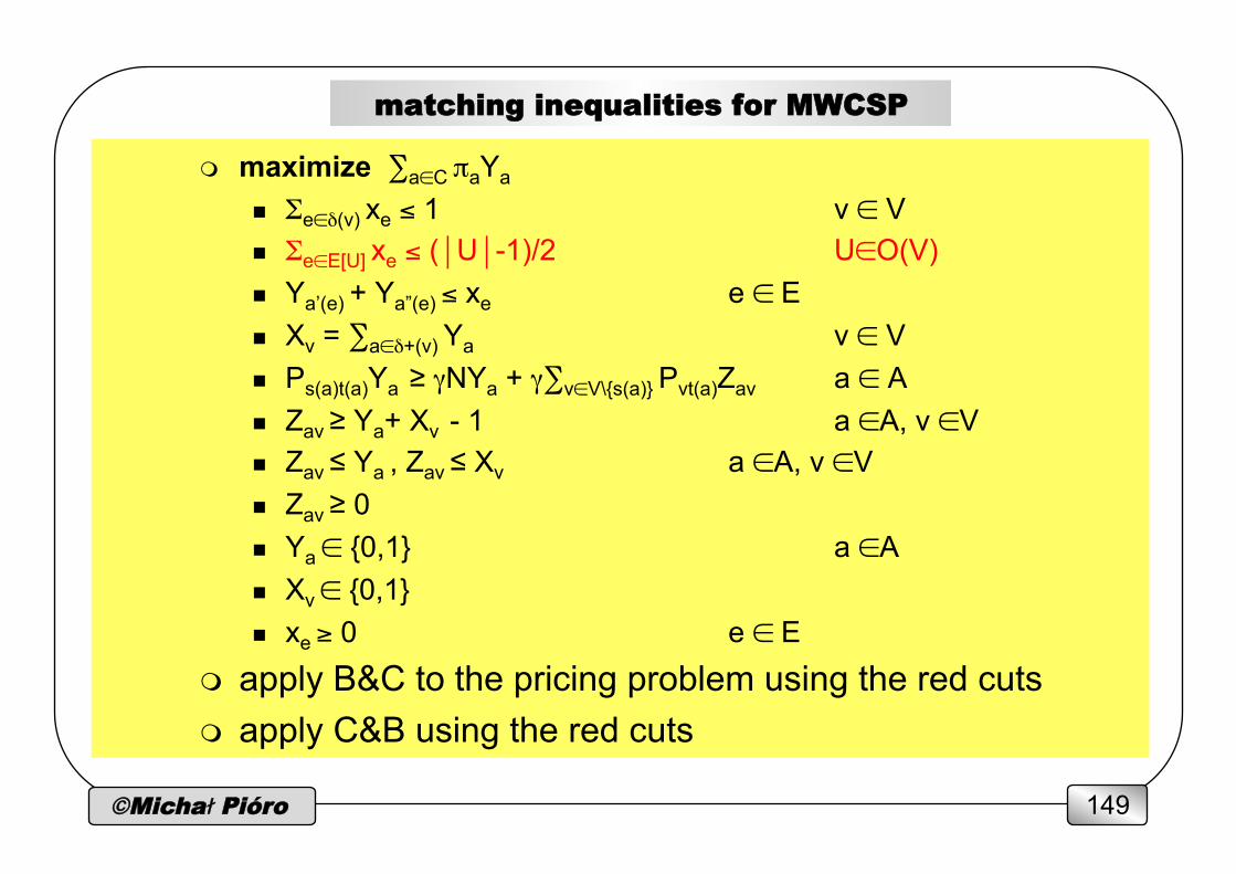
matching inequalities for MWCSP
m maximize ∑a∈C πaYa
n Σe∈δ(v) xe ≤ 1 v ∈ V n Σe∈E[U] xe ≤ (⏐U⏐-1)/2 U∈O(V) n Ya’(e) + Ya”(e) ≤ xe e ∈ E n Xv = ∑a∈δ+(v) Ya v ∈ V n Ps(a)t(a)Ya ≥ γNYa + γ∑v∈V\{s(a)} Pvt(a)Zav a ∈ A n Zav ≥ Ya+ Xv - 1 a ∈A, v ∈V n Zav ≤ Ya , Zav ≤ Xv a ∈A, v ∈V n Zav ≥ 0 n Ya ∈ {0,1} a ∈A n Xv ∈ {0,1} n xe ≥ 0 e ∈ E
m apply B&C to the pricing problem using the red cuts m apply C&B using the red cuts
©Michał Pióro 150
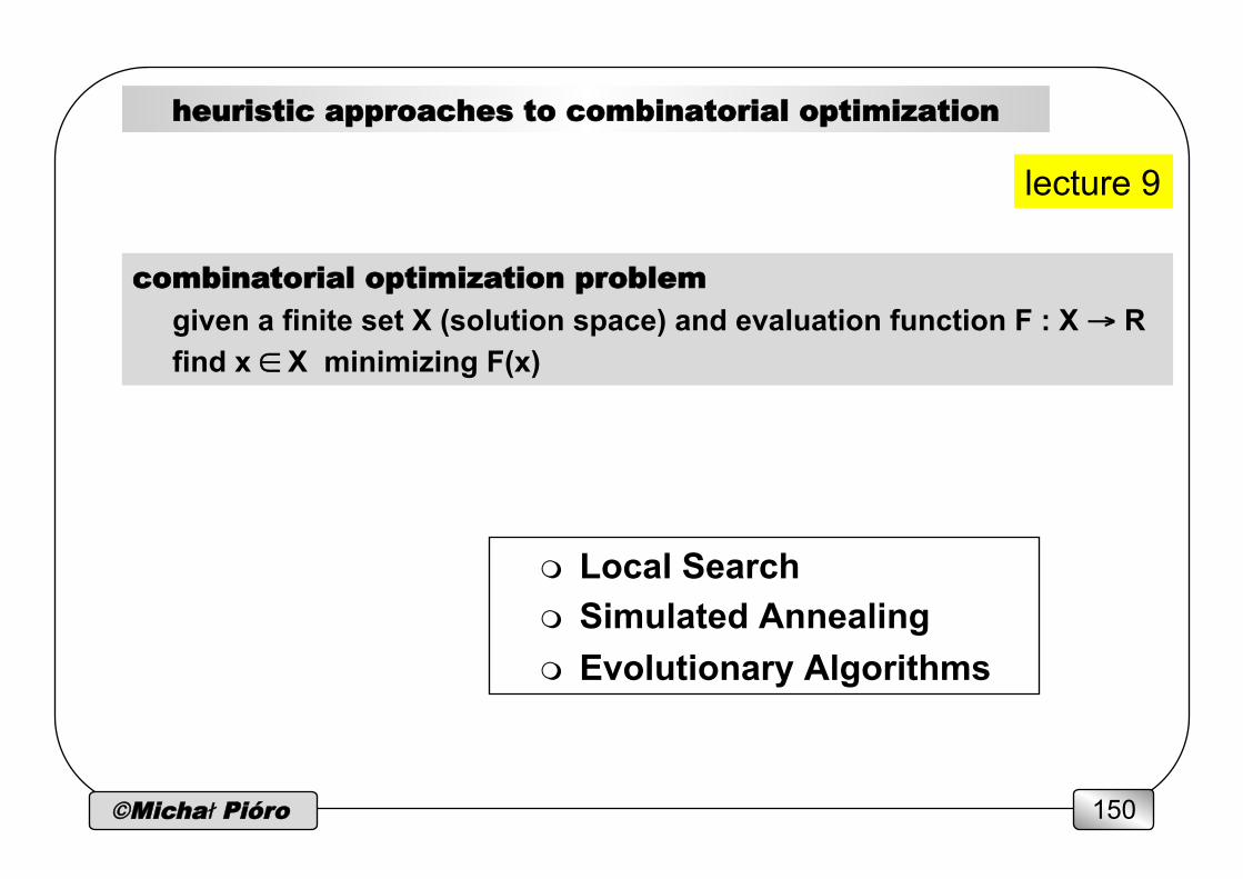
heuristic approaches to combinatorial optimization
m Local Search m Simulated Annealing m Evolutionary Algorithms
combinatorial optimization problem
given a finite set X (solution space) and evaluation function F : X → R find x ∈ X minimizing F(x)
lecture 9
©Michał Pióro 151
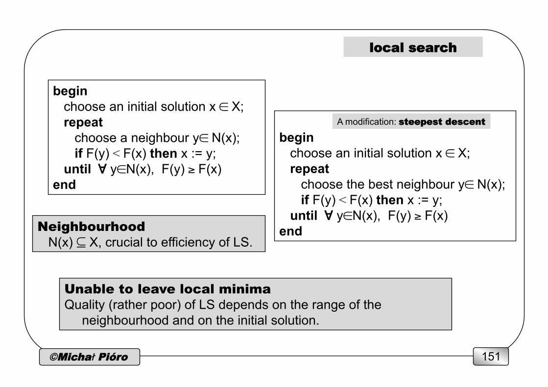
local search
begin choose an initial solution x ∈ X; repeat choose the best neighbour y∈ N(x); if F(y) < F(x) then x := y; until ∀ y∈N(x), F(y) ≥ F(x) end
begin choose an initial solution x ∈ X; repeat choose a neighbour y∈ N(x); if F(y) < F(x) then x := y; until ∀ y∈N(x), F(y) ≥ F(x) end
A modification: steepest descent
Unable to leave local minima Quality (rather poor) of LS depends on the range of the
neighbourhood and on the initial solution.
Neighbourhood N(x) ⊆ X, crucial to efficiency of LS.
©Michał Pióro 152
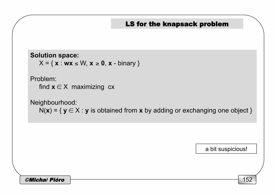
LS for the knapsack problem
Solution space: X = { x : wx ≤ W, x ≥ 0, x - binary }
Problem:
find x ∈ X maximizing cx Neighbourhood:
N(x) = { y ∈ X : y is obtained from x by adding or exchanging one object }
a bit suspicious!
©Michał Pióro 153
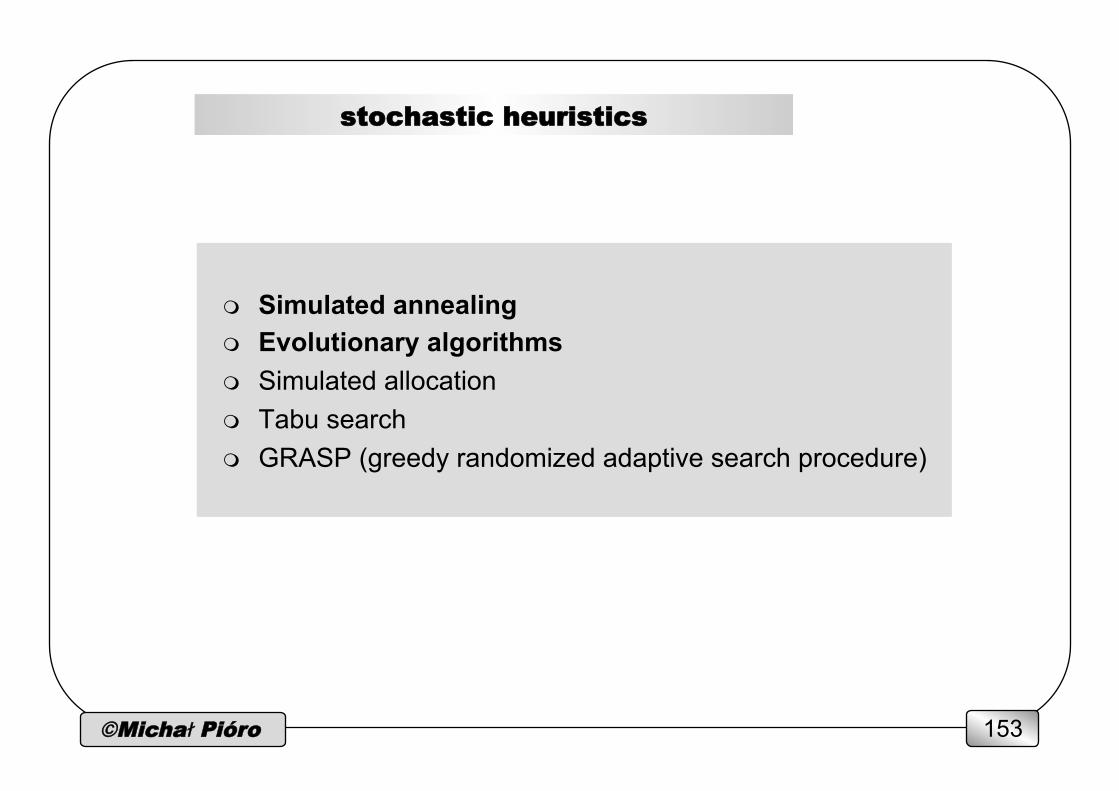
stochastic heuristics
m Simulated annealing m Evolutionary algorithms m Simulated allocation m Tabu search m GRASP (greedy randomized adaptive search procedure)
©Michał Pióro 154
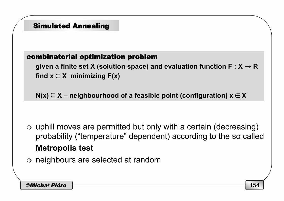
Simulated Annealing
m uphill moves are permitted but only with a certain (decreasing) probability (“temperature” dependent) according to the so called Metropolis test
m neighbours are selected at random
combinatorial optimization problem given a finite set X (solution space) and evaluation function F : X → R find x ∈ X minimizing F(x)
N(x) ⊆ X – neighbourhood of a feasible point (configuration) x ∈ X
©Michał Pióro 155
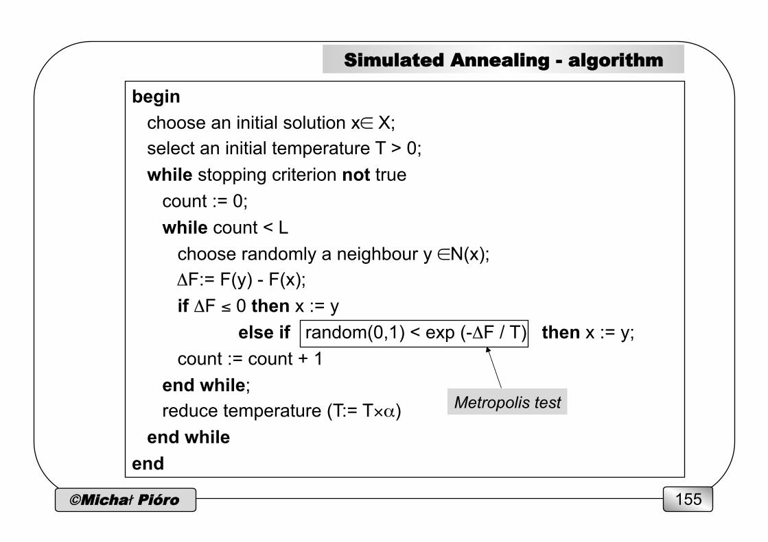
Simulated Annealing - algorithm
begin choose an initial solution x∈ X; select an initial temperature T > 0; while stopping criterion not true count := 0; while count < L choose randomly a neighbour y ∈N(x); ΔF:= F(y) - F(x); if ΔF ≤ 0 then x := y else if random(0,1) < exp (-ΔF / T) then x := y; count := count + 1 end while; reduce temperature (T:= T×α) end while end
Metropolis test

©Michał Pióro 156
Simulated Annealing - limit theorem
m limit theorem: global optimum will be found m for fixed T, after sufficiently number of steps:
n Prob { S = x } = exp(-F(x)/T) / Z(T) n Z(T) = Σy∈X exp(-F(y)/T)
m for T→0, Prob { S = x } remains greater than 0 only for optimal configurations i∈S, see [Ber98]
this is not a very practical result: too many moves (number of states squared) would have to be made to achieve the limit sufficiently closely
[Ber98] D.P. Bertsekas Network Optimization: Continuous and Discrete Models. Athena Scientific, 1998.
©Michał Pióro 157
Simulated Annealing applied to the Travelling Salesman Problem (TSP)
Combinatorial Optimisation Problem given a finite set X (solution space) and evaluation function F : X → R find x ∈ X minimizing F(x), N(x) ⊆ X - neighbourhood of a feasible point (configuration) x ∈ X
TSP X = { x : set of all Hamiltonian cycles in a fully connected graph } N(x) - neighbourhood of x (next slide) Find a shortest Hamiltonian cycle (road distance)
©Michał Pióro 158
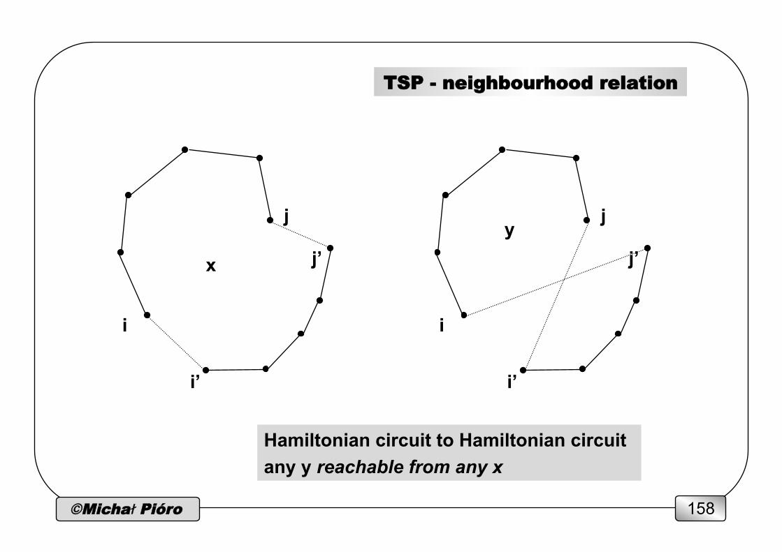
TSP - neighbourhood relation
Hamiltonian circuit to Hamiltonian circuit any y reachable from any x
i
j’
i’
j
i
j’
i’
j y
x
©Michał Pióro 159
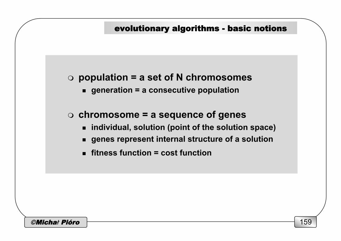
m population = a set of N chromosomes n generation = a consecutive population
m chromosome = a sequence of genes n individual, solution (point of the solution space) n genes represent internal structure of a solution n fitness function = cost function
evolutionary algorithms - basic notions

©Michał Pióro 160
m mutation n is performed over a chromosome with certain (low)
probability n it perturbs the values of the chromosome’s genes
m crossover n exchanges genes between two parent chromosomes to
produce an offspring n in effect the offspring has genes from both parents n chromosomes with better fitness function have greater
chance to become parents
genetic operators
in general, the operators are problem-dependent
©Michał Pióro 161
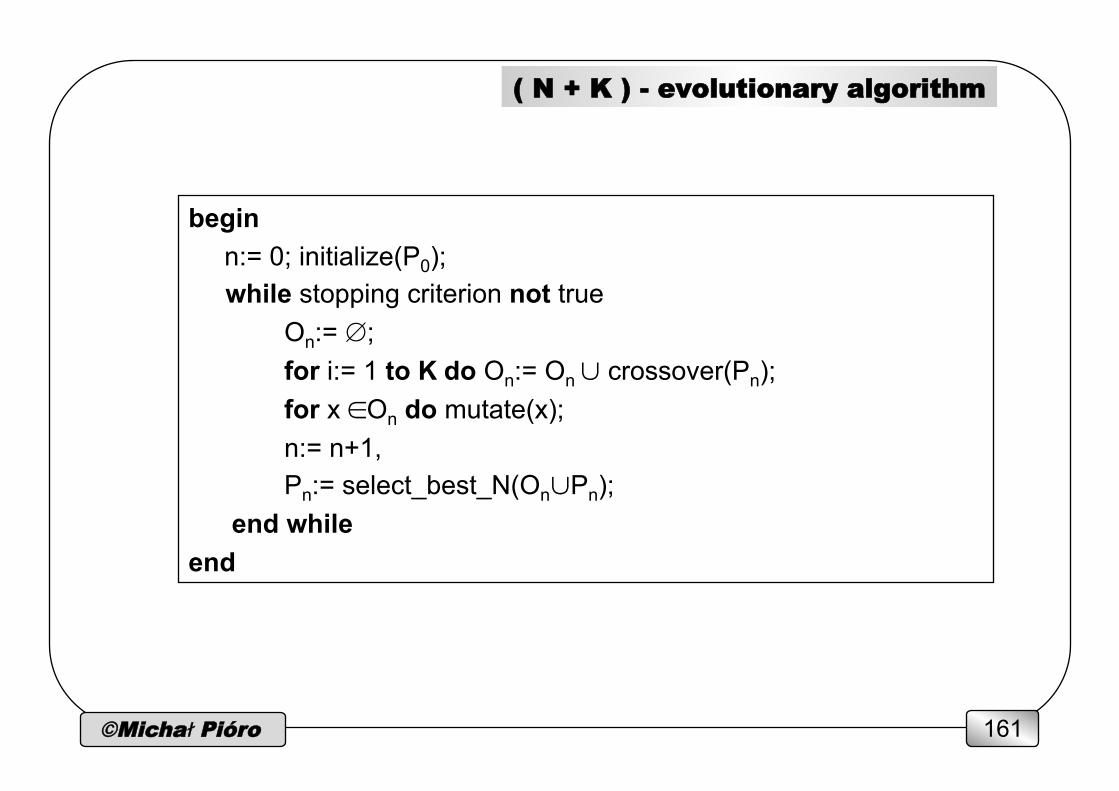
( N + K ) - evolutionary algorithm
begin n:= 0; initialize(P0); while stopping criterion not true On:= ∅; for i:= 1 to K do On:= On ∪ crossover(Pn);
for x ∈On do mutate(x); n:= n+1,
Pn:= select_best_N(On∪Pn); end while end
©Michał Pióro 162
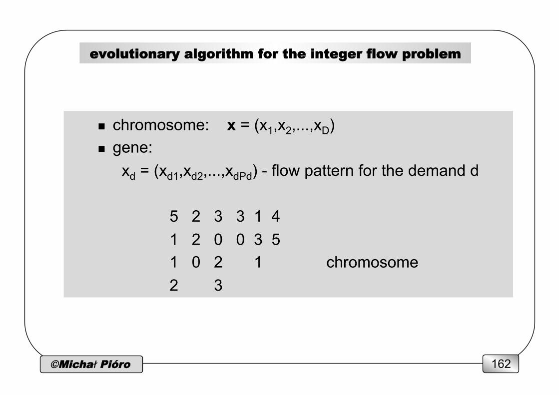
n chromosome: x = (x1,x2,...,xD) n gene:
xd = (xd1,xd2,...,xdPd) - flow pattern for the demand d
5 2 3 3 1 4 1 2 0 0 3 5 1 0 2 1 chromosome 2 3
evolutionary algorithm for the integer flow problem

©Michał Pióro 163
evolutionary algorithm for the flow problem (cntd.)
m crossover of two chromosomes n each gene of the offspring is taken from one of the parents
❏ for each d=1,2,…,D: xd := xd(1) with probability 0.5 xd := xd(2) with probability 0.5
n better fitted chromosomes have greater chance to become parents
m mutation of a chromosome n for each gene shift some flow from one path to another n everything at random
Think how to approach this problem with simulated annealing?
©Michał Pióro 164
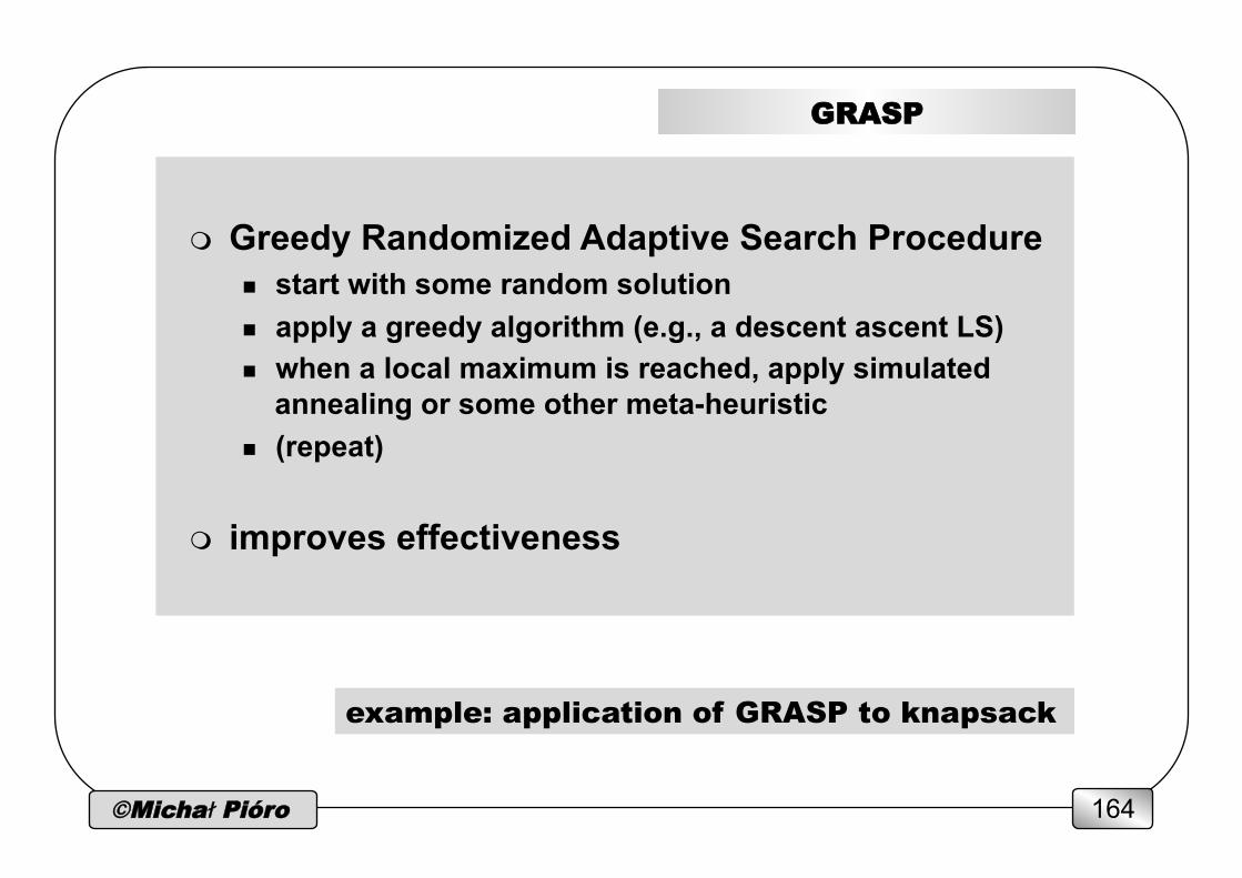
m Greedy Randomized Adaptive Search Procedure n start with some random solution n apply a greedy algorithm (e.g., a descent ascent LS) n when a local maximum is reached, apply simulated
annealing or some other meta-heuristic n (repeat)
m improves effectiveness
GRASP
example: application of GRASP to knapsack
©Michał Pióro 165
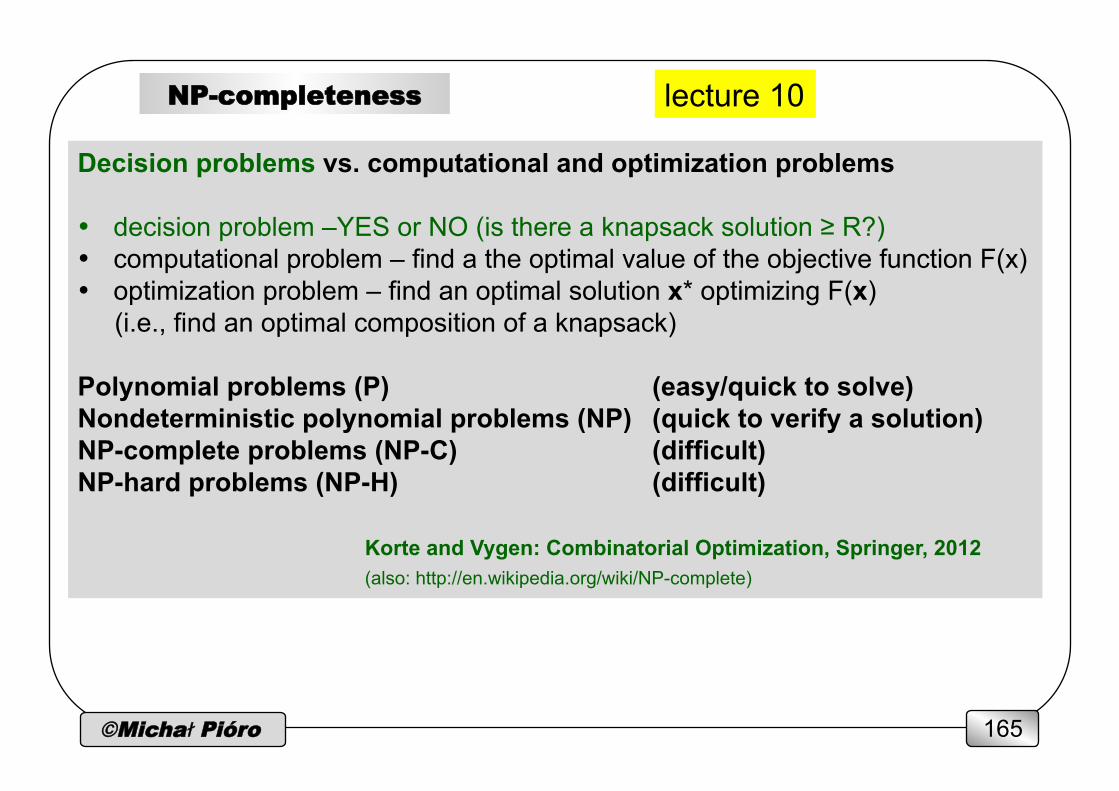
Decision problems vs. computational and optimization problems
• decision problem –YES or NO (is there a knapsack solution ≥ R?) • computational problem – find a the optimal value of the objective function F(x) • optimization problem – find an optimal solution x* optimizing F(x) (i.e., find an optimal composition of a knapsack) Polynomial problems (P) (easy/quick to solve) Nondeterministic polynomial problems (NP) (quick to verify a solution) NP-complete problems (NP-C) (difficult) NP-hard problems (NP-H) (difficult)
Korte and Vygen: Combinatorial Optimization, Springer, 2012 (also: http://en.wikipedia.org/wiki/NP-complete)
NP-completeness lecture 10

©Michał Pióro 166
HC: Given a graph, find a cycle going through all nodes (exactly once
through each node). TSP: In a weighted graph, find a shortest HC (travelling salesman problem).
Decision versions: • Does there exist a Hamiltonian cycle? • Does there exist w Hamiltonian cycle of length between C1 and C2?
Hamiltonian cycle problem (HCP)
©Michał Pióro 167
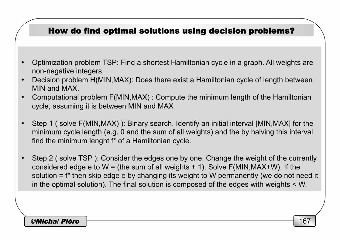
How do find optimal solutions using decision problems?
• Optimization problem TSP: Find a shortest Hamiltonian cycle in a graph. All weights are
non-negative integers. • Decision problem H(MIN,MAX): Does there exist a Hamiltonian cycle of length between
MIN and MAX. • Computational problem F(MIN,MAX) : Compute the minimum length of the Hamiltonian
cycle, assuming it is between MIN and MAX
• Step 1 ( solve F(MIN,MAX) ): Binary search. Identify an initial interval [MIN,MAX] for the minimum cycle length (e.g. 0 and the sum of all weights) and the by halving this interval find the minimum lenght f* of a Hamiltonian cycle.
• Step 2 ( solve TSP ): Consider the edges one by one. Change the weight of the currently
considered edge e to W = (the sum of all weights + 1). Solve F(MIN,MAX+W). If the solution = f* then skip edge e by changing its weight to W permanently (we do not need it in the optimal solution). The final solution is composed of the edges with weights < W.
©Michał Pióro 168
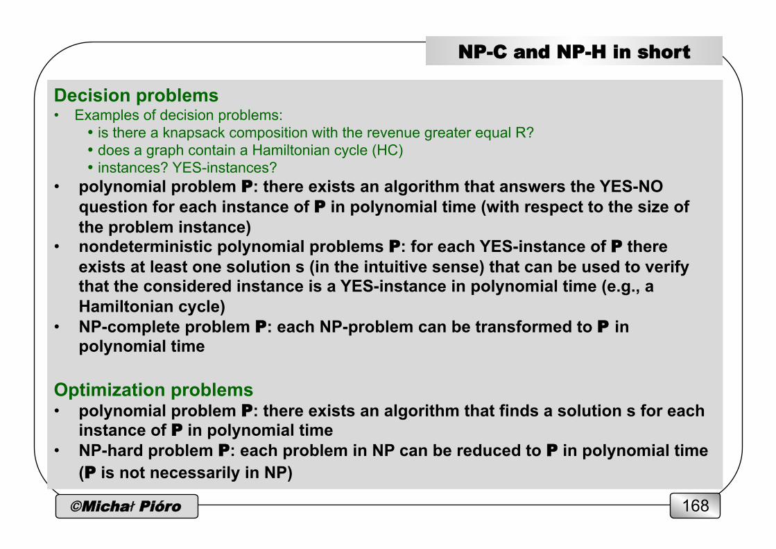
Decision problems • Examples of decision problems:
• is there a knapsack composition with the revenue greater equal R? • does a graph contain a Hamiltonian cycle (HC) • instances? YES-instances?
• polynomial problem P: there exists an algorithm that answers the YES-NO question for each instance of P in polynomial time (with respect to the size of the problem instance)
• nondeterministic polynomial problems P: for each YES-instance of P there exists at least one solution s (in the intuitive sense) that can be used to verify that the considered instance is a YES-instance in polynomial time (e.g., a Hamiltonian cycle)
• NP-complete problem P: each NP-problem can be transformed to P in polynomial time
Optimization problems • polynomial problem P: there exists an algorithm that finds a solution s for each
instance of P in polynomial time • NP-hard problem P: each problem in NP can be reduced to P in polynomial time
(P is not necessarily in NP)
NP-C and NP-H in short
©Michał Pióro 169
decision problems
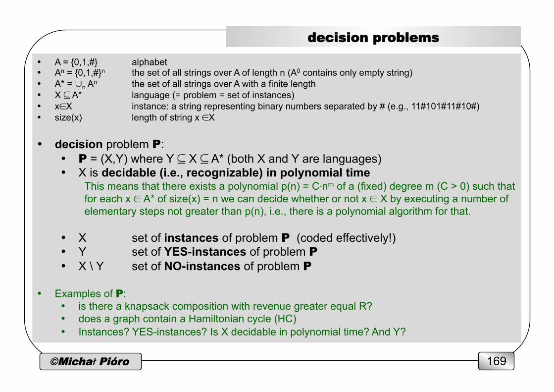
• A = {0,1,#} alphabet • An = {0,1,#}n the set of all strings over A of length n (A0 contains only empty string) • A* = ∪n An the set of all strings over A with a finite length • X ⊆ A* language (= problem = set of instances) • x∈X instance: a string representing binary numbers separated by # (e.g., 11#101#11#10#) • size(x) length of string x ∈X
• decision problem P: • P = (X,Y) where Y ⊆ X ⊆ A* (both X and Y are languages) • X is decidable (i.e., recognizable) in polynomial time
This means that there exists a polynomial p(n) = C⋅nm of a (fixed) degree m (C > 0) such that for each x ∈ A* of size(x) = n we can decide whether or not x ∈ X by executing a number of elementary steps not greater than p(n), i.e., there is a polynomial algorithm for that.
• X set of instances of problem P (coded effectively!) • Y set of YES-instances of problem P • X \ Y set of NO-instances of problem P
• Examples of P: • is there a knapsack composition with revenue greater equal R? • does a graph contain a Hamiltonian cycle (HC) • Instances? YES-instances? Is X decidable in polynomial time? And Y?
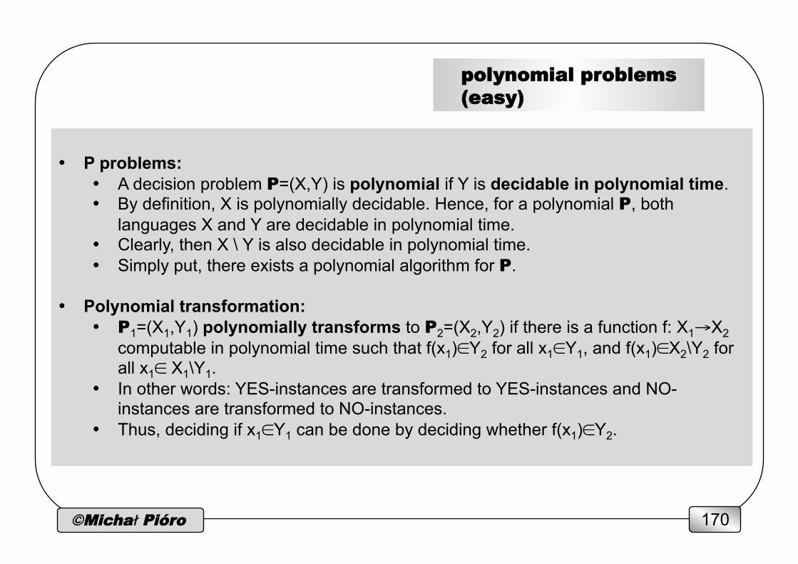
©Michał Pióro 170
• P problems:
• A decision problem P=(X,Y) is polynomial if Y is decidable in polynomial time. • By definition, X is polynomially decidable. Hence, for a polynomial P, both
languages X and Y are decidable in polynomial time. • Clearly, then X \ Y is also decidable in polynomial time. • Simply put, there exists a polynomial algorithm for P.
• Polynomial transformation: • P1=(X1,Y1) polynomially transforms to P2=(X2,Y2) if there is a function f: X1→X2
computable in polynomial time such that f(x1)∈Y2 for all x1∈Y1, and f(x1)∈X2\Y2 for all x1∈ X1\Y1.
• In other words: YES-instances are transformed to YES-instances and NO-instances are transformed to NO-instances.
• Thus, deciding if x1∈Y1 can be done by deciding whether f(x1)∈Y2.
polynomial problems (easy)
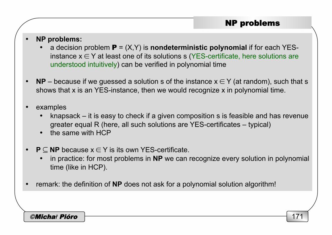
©Michał Pióro 171
NP problems
• NP problems: • a decision problem P = (X,Y) is nondeterministic polynomial if for each YES-
instance x ∈ Y at least one of its solutions s (YES-certificate, here solutions are understood intuitively) can be verified in polynomial time
• NP – because if we guessed a solution s of the instance x ∈ Y (at random), such that s shows that x is an YES-instance, then we would recognize x in polynomial time.
• examples • knapsack – it is easy to check if a given composition s is feasible and has revenue
greater equal R (here, all such solutions are YES-certificates – typical) • the same with HCP
• P ⊆ NP because x ∈ Y is its own YES-certificate. • in practice: for most problems in NP we can recognize every solution in polynomial
time (like in HCP). • remark: the definition of NP does not ask for a polynomial solution algorithm!
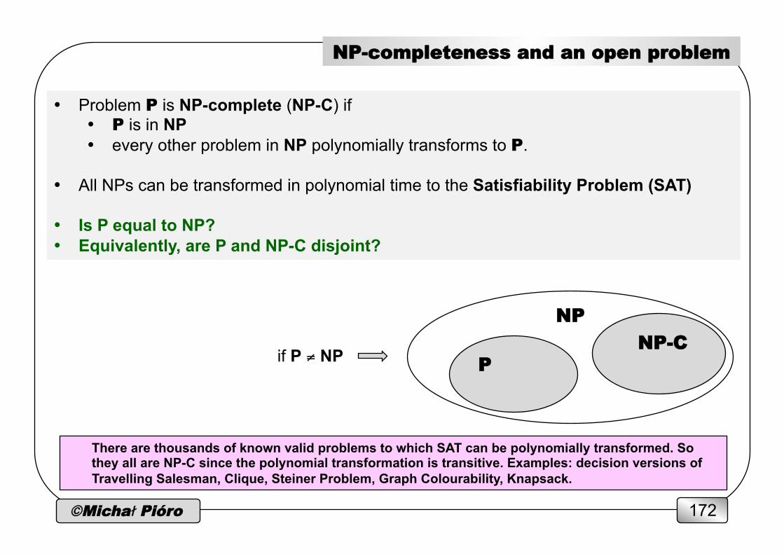
©Michał Pióro 172
NP-completeness and an open problem
• Problem P is NP-complete (NP-C) if • P is in NP • every other problem in NP polynomially transforms to P.
• All NPs can be transformed in polynomial time to the Satisfiability Problem (SAT)
• Is P equal to NP? • Equivalently, are P and NP-C disjoint?
P
NP NP-C
There are thousands of known valid problems to which SAT can be polynomially transformed. So they all are NP-C since the polynomial transformation is transitive. Examples: decision versions of Travelling Salesman, Clique, Steiner Problem, Graph Colourability, Knapsack.
if P ≠ NP
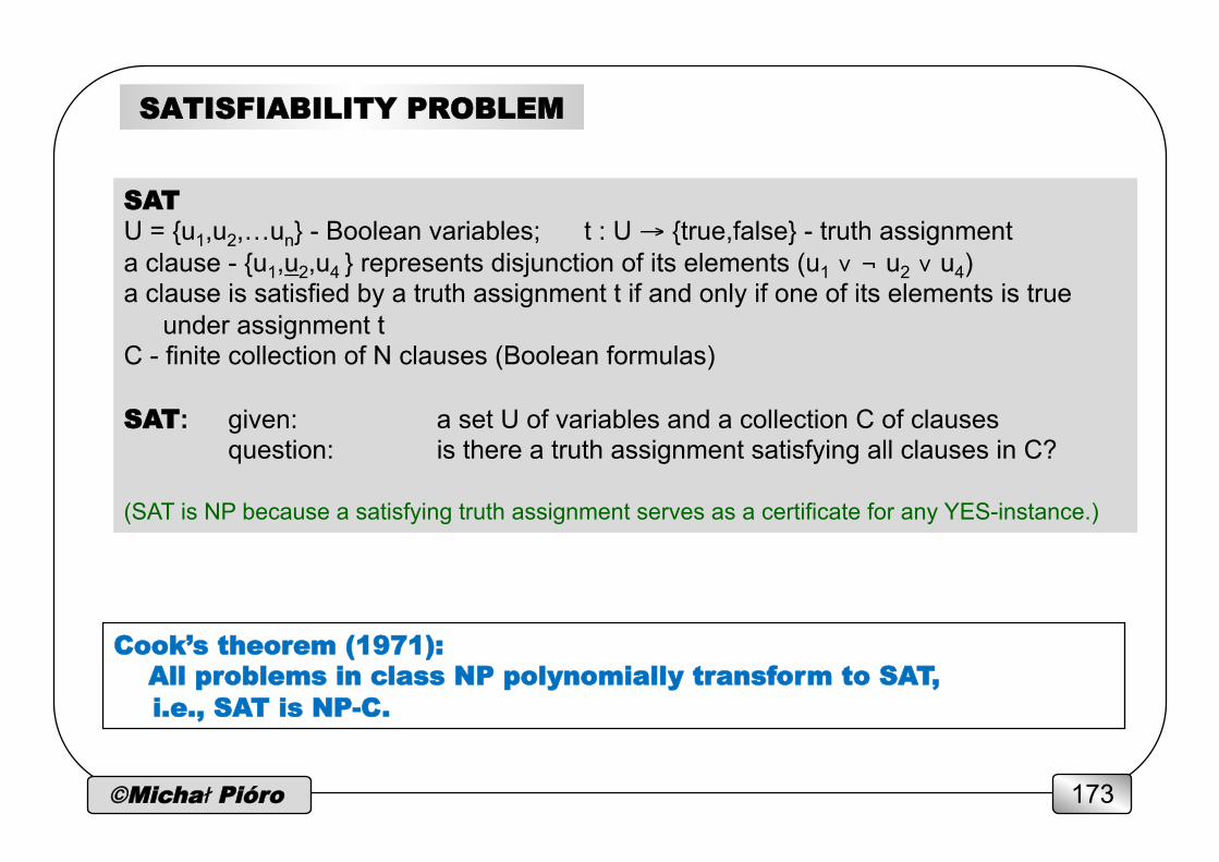
©Michał Pióro 173
SATISFIABILITY PROBLEM
SAT U = {u1,u2,…un} - Boolean variables; t : U → {true,false} - truth assignment a clause - {u1,u2,u4 } represents disjunction of its elements (u1 ∨ ¬ u2 ∨ u4) a clause is satisfied by a truth assignment t if and only if one of its elements is true
under assignment t C - finite collection of N clauses (Boolean formulas) SAT: given: a set U of variables and a collection C of clauses
question: is there a truth assignment satisfying all clauses in C? (SAT is NP because a satisfying truth assignment serves as a certificate for any YES-instance.)
Cook’s theorem (1971): All problems in class NP polynomially transform to SAT,
i.e., SAT is NP-C.
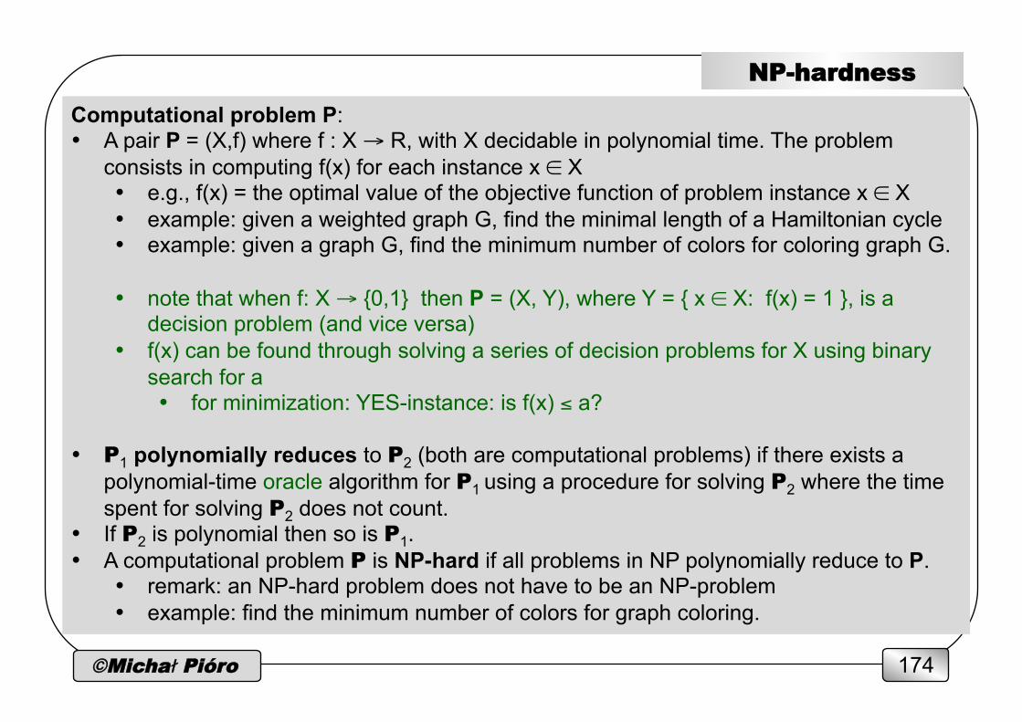
©Michał Pióro 174
NP-hardness
Computational problem P: • A pair P = (X,f) where f : X → R, with X decidable in polynomial time. The problem
consists in computing f(x) for each instance x ∈ X • e.g., f(x) = the optimal value of the objective function of problem instance x ∈ X • example: given a weighted graph G, find the minimal length of a Hamiltonian cycle • example: given a graph G, find the minimum number of colors for coloring graph G.
• note that when f: X → {0,1} then P = (X, Y), where Y = { x ∈ X: f(x) = 1 }, is a decision problem (and vice versa)
• f(x) can be found through solving a series of decision problems for X using binary search for a • for minimization: YES-instance: is f(x) ≤ a?
• P1 polynomially reduces to P2 (both are computational problems) if there exists a polynomial-time oracle algorithm for P1 using a procedure for solving P2 where the time spent for solving P2 does not count.
• If P2 is polynomial then so is P1. • A computational problem P is NP-hard if all problems in NP polynomially reduce to P.
• remark: an NP-hard problem does not have to be an NP-problem • example: find the minimum number of colors for graph coloring.
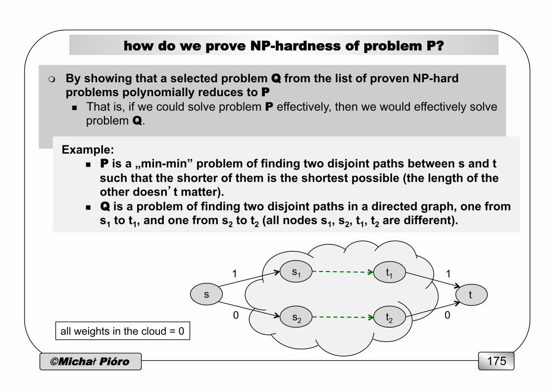
©Michał Pióro 175
how do we prove NP-hardness of problem P?
m By showing that a selected problem Q from the list of proven NP-hard problems polynomially reduces to P n That is, if we could solve problem P effectively, then we would effectively solve
problem Q.
Example: n P is a „min-min” problem of finding two disjoint paths between s and t
such that the shorter of them is the shortest possible (the length of the other doesn’t matter).
n Q is a problem of finding two disjoint paths in a directed graph, one from s1 to t1, and one from s2 to t2 (all nodes s1, s2, t1, t2 are different).
s t1
s t
s t2
s s1
s s2
1
0
1
0 all weights in the cloud = 0
©Michał Pióro 176
IP (and MIP) is NP-hard
m SATISFIABILTY PROBLEM (SAT) can be expressed as IP m even as a binary program (all integer variables are binary)
Every real-life problem can be modeled (with a sufficient accuracy) as a MIP!
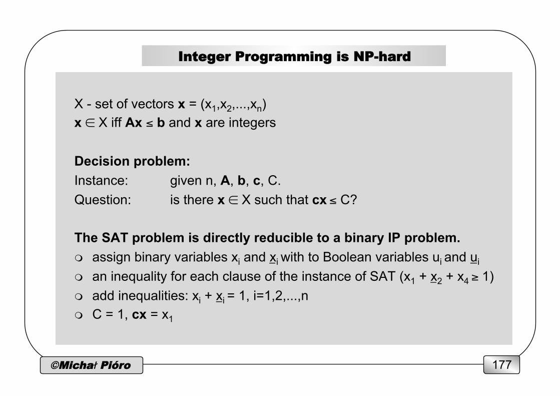
©Michał Pióro 177
X - set of vectors x = (x1,x2,...,xn) x ∈ X iff Ax ≤ b and x are integers Decision problem: Instance: given n, A, b, c, C. Question: is there x ∈ X such that cx ≤ C? The SAT problem is directly reducible to a binary IP problem. m assign binary variables xi and xi with to Boolean variables ui and ui
m an inequality for each clause of the instance of SAT (x1 + x2 + x4 ≥ 1) m add inequalities: xi + xi = 1, i=1,2,...,n m C = 1, cx = x1
Integer Programming is NP-hard
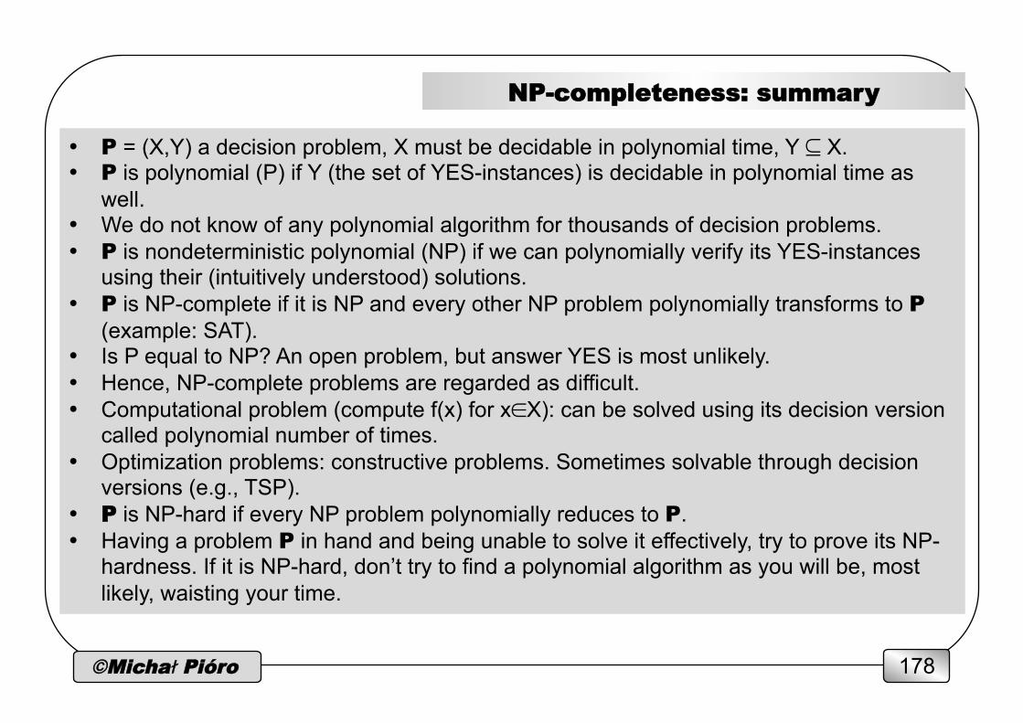
©Michał Pióro 178
• P = (X,Y) a decision problem, X must be decidable in polynomial time, Y ⊆ X. • P is polynomial (P) if Y (the set of YES-instances) is decidable in polynomial time as
well. • We do not know of any polynomial algorithm for thousands of decision problems. • P is nondeterministic polynomial (NP) if we can polynomially verify its YES-instances
using their (intuitively understood) solutions. • P is NP-complete if it is NP and every other NP problem polynomially transforms to P
(example: SAT). • Is P equal to NP? An open problem, but answer YES is most unlikely. • Hence, NP-complete problems are regarded as difficult. • Computational problem (compute f(x) for x∈X): can be solved using its decision version
called polynomial number of times. • Optimization problems: constructive problems. Sometimes solvable through decision
versions (e.g., TSP). • P is NP-hard if every NP problem polynomially reduces to P. • Having a problem P in hand and being unable to solve it effectively, try to prove its NP-
hardness. If it is NP-hard, don’t try to find a polynomial algorithm as you will be, most likely, waisting your time.
NP-completeness: summary
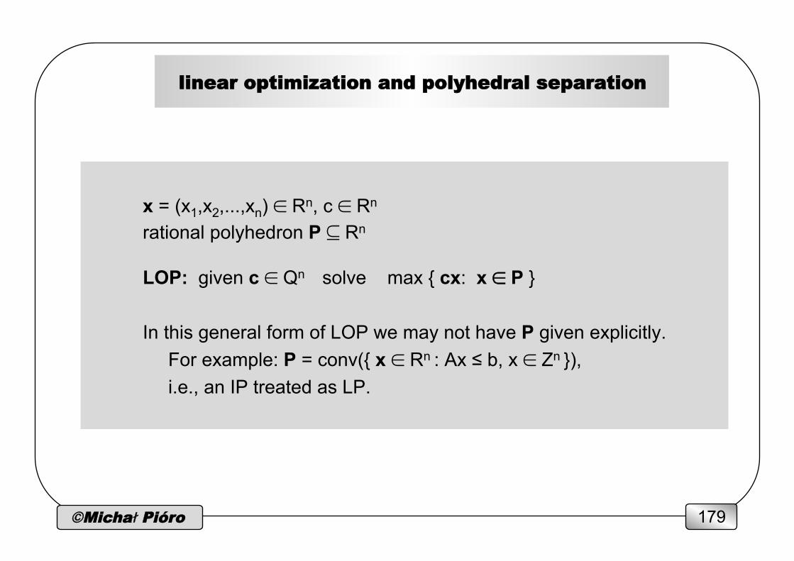
©Michał Pióro 179
x = (x1,x2,...,xn) ∈ Rn, c ∈ Rn rational polyhedron P ⊆ Rn
LOP: given c ∈ Qn solve max { cx: x ∈ P } In this general form of LOP we may not have P given explicitly.
For example: P = conv({ x ∈ Rn : Ax ≤ b, x ∈ Zn }), i.e., an IP treated as LP.
linear optimization and polyhedral separation
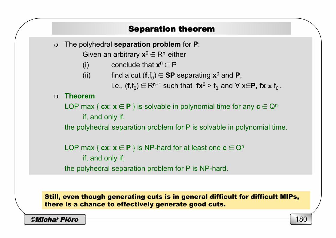
©Michał Pióro 180
Separation theorem
m The polyhedral separation problem for P: Given an arbitrary x0 ∈ Rn either (i) conclude that x0 ∈ P (ii) find a cut (f,f0) ∈ SP separating x0 and P, i.e., (f,f0) ∈ Rn+1 such that fx0 > f0 and ∀ x∈P, fx ≤ f0 .
m Theorem LOP max { cx: x ∈ P } is solvable in polynomial time for any c ∈ Qn
if, and only if, the polyhedral separation problem for P is solvable in polynomial time.
LOP max { cx: x ∈ P } is NP-hard for at least one c ∈ Qn
if, and only if, the polyhedral separation problem for P is NP-hard.
Still, even though generating cuts is in general difficult for difficult MIPs, there is a chance to effectively generate good cuts.
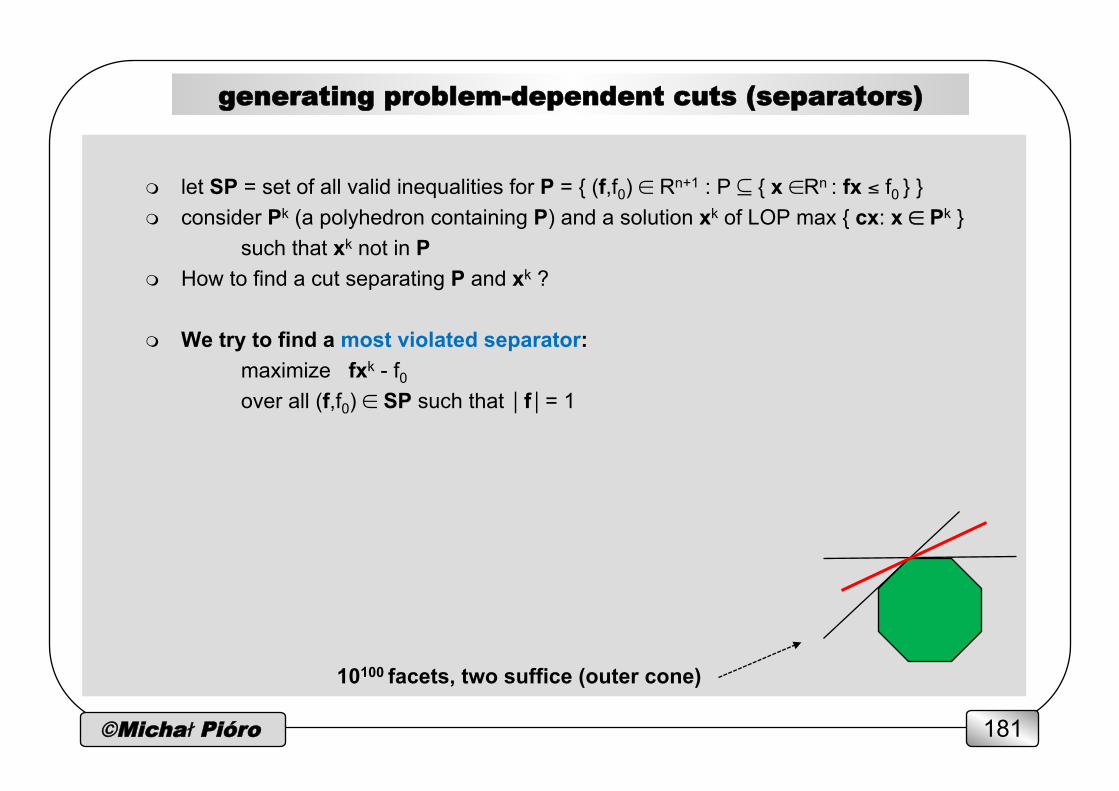
©Michał Pióro 181
generating problem-dependent cuts (separators)
m let SP = set of all valid inequalities for P = { (f,f0) ∈ Rn+1 : P ⊆ { x ∈Rn : fx ≤ f0 } } m consider Pk (a polyhedron containing P) and a solution xk of LOP max { cx: x ∈ Pk }
such that xk not in P m How to find a cut separating P and xk ? m We try to find a most violated separator:
maximize fxk - f0 over all (f,f0) ∈ SP such that ⎥ f⎥ = 1
10100 facets, two suffice (outer cone)
©Michał Pióro 182
Why LPs, MIPs, and IPs are so important?
m in practice only LPs guarantee efficient solutions n decomposition methods are available for LPs (e.g., path generation) n convex problems can be approximated by LPs
m all real-life problems can be expressed as MIPs n concave objective functions can be approximated by MIPs
m MIPs and IPs can be solved by general solvers by branch-and-bound method (and its enhancements B&C, B&P, C&B, B&P&C), based on LP n CPLEX, XPRESS, Gurobi n sometimes efficiently
m otherwise, we have to use (frequently) unreliable stochastic meta-heuristics (sometimes specialized heuristics) n a good heuristic solution (i.e., a suboptimal MIP solution F*: initial zbest)
leads to improved branching (at a B&B node: F(x) ≥ F*)

©Michał Pióro 183
important topics not discussed
m multi-state network design n taking failure states into account n multi-hour design n multi-period dsign
m multi-layer network design m traffic uncertainty
n polyhdral approach (robust optimization) n stochastic programming
m including fairness to network design m shortest-path routing m ...
the end