algorithms to find two–hop routing policies in multi–class delay tolerant...

1

Algorithms to Find Two–Hop Routing Policies inMulti–Class Delay Tolerant Networks

Nicola Basilico, Matteo Cesana, Member, IEEE, and Nicola Gatti

Abstract—Most of the literature on Delay Tolerant Networks(DTNs) focuses on optimal routing policies exploiting a prioriknowledge about nodes mobility traces. For the case in whichno a priori knowledge is available (very common in practice),apart from basic epidemic routing, the main approaches focuson controlling two–hop routing policies. However, these latterresults commonly employ fluid approximation techniques, which,in principle, do not provide any theoretical bound over theapproximation ratio. In our work, we focus on the case withouta priori mobility knowledge and we provide approximationalgorithms with theoretical guarantees that can be applied tocases where the number of hops allowed in the routing process isarbitrary. Our approach is rather flexible allowing us to addressheterogeneous mobility patterns and transmission technologies,to consider explicitly the signaling and transmission costs, andto include also nodes discarding packets after a local timeout.We then provide a comprehensive performance evaluation ofour algorithms, showing that two–hop routing provides the besttradeoff between delay and energy and that, in this case, theyfind solutions very close to the optimal ones with a low overhead.Finally, we compare our methods against some state–of–the–art approaches by means of a DTN simulation environment inrealistic settings.

I. INTRODUCTION

DTNs are sparse and/or highly mobile wireless ad hocnetworks with discontinuous connectivity, which may

occur due to limits in the wireless radio range, sparsity ofmobile nodes, constrained energy resources, attacks, and noise.One central problem in DTNs is the optimal routing of packetsfrom a source towards the desired destinations.

When no a priori information is available on the mobilitypattern of the nodes, a common technique for overcominglack of connectivity is to disseminate multiple copies of thepacket: this enhances the probability that at least one ofthem will reach the destination within a temporal deadline.This is referred to as epidemic–style forwarding, because,alike the spread of infectious diseases, each time a packet–carrying node encounters a new node not having a copythereof, the carrier may infect this new node by passing ona packet copy. A convenient compromise of energy versusdelay compared to epidemic routing is provided by two–hoprouting where the infection is limited to contacts between thesource and intermediary nodes, that is, the source node passeson the packets to all the mobile nodes she encounters, andthe “infected” mobile nodes can deliver the packets they arecarrying only to the final destination.

N. Basilico is with the Department of Computer Science, University ofMilan, Milan, Italy, E-mail: [email protected].

M. Cesana and N. Gatti are with the Dipartimento di Elettronica, In-formazione e Bioingegneria, Politecnico di Milano, Milano, Italy, E-mail:matteo.cesana, [email protected].

In this paper, we focus on the characterization of two–hoprouting policies for DTNs as in [1]–[3], where the problemconcerns the decision on whether or not forwarding a givenpacket to a given mobile node the source is encountering ata given time. We propose an optimization-based frameworkto derive optimal two–hop routing policies which extends theavailable approaches in the literature in different directions:(i) we account for mobile nodes which are categorized indistinct multiple classes capturing different mobility patternsand available communication technologies on board; (ii) weaccount for the cost for neighbor discovery and signalingmessages exchange to support packet forwarding further al-lowing mobile nodes to discard the packets they are carryingupon expiration of a local temporal deadline; (iii) rather thanresorting to fluid approximation to derive optimal two–hoprouting policies, we propose algorithms for finite mobile nodepopulations with theoretical guarantees; namely we providean exponential–time (in the number of classes) algorithm tofind routing policies that are arbitrarily close to the optimalones, as well as approximate polynomial–time algorithms; (iv)we extend our algorithms and analysis to the case wherethe routing policy allows an arbitrary maximum number ofhops. Finally, we provide a thorough performance evaluationwith realistic settings of the proposed algorithms in termsof approximation ratio, scalability in the number of classes,further evaluating the impact of network parameters onto theoptimal routing policies. We also evaluate our routing policieswith different maximum numbers of allowed hops and wecompare them w.r.t. state–of–the–art routing policies withinThe ONE Simulator [4].

The paper is organized as follows. Section II reviews therelevant literature. Sections III and IV describe the referencescenario and routing problem. Our approximation algorithmsare presented in Section V while extensions to more thantwo hops is addressed in Section VI. Section VII, evaluatesalgorithms in synthetic network instances while Section VIIIconcludes the paper.

II. RELATED WORK

The main distinctive features of the present work w.r.t.the reference literature are: (i) we take into account the costfor neighbor discovery and signaling messages exchange tosupport packet forwarding, further allowing mobile nodes todiscard ”older” packets upon expiration of a local temporaldeadline (implying that, differently from what customarilyassumed in the reference literature, the number of copies ofa packet is not monotone–increasing); (ii) we do not resortto fluid approximation, but rather propose algorithms to find

This is the author's version of an article that has been published in this journal. Changes were made to this version by the publisher prior to publication.The final version of record is available at http://dx.doi.org/10.1109/TWC.2016.2532859

Copyright (c) 2016 IEEE. Personal use is permitted. For any other purposes, permission must be obtained from the IEEE by emailing [email protected].

2

optimal routing policies for finite mobile node populationswith theoretical performance guarantees; (iii) we extend ouralgorithms to the case where the number of hops allowed inthe routing phase is arbitrary; (iv) we compare our algorithmsw.r.t. state–of–the–art algorithms by means of one of the mainDTN simulators.

We overview here the main body of literature in the fields ofoptimizing multi–hop routing and two–hop routing in DTNs.

Multi–Hop Routing. Besides basic epidemic–style forward-ing schemes operating under a zero–information assumption(in Section VII-E we briefly review and compare againstthem), literature on optimal routing mainly devoted efforts inscenarios where some knowledge about mobility is availableand can be exploited. The seminal work [5] studies optimalmulti–hop routing strategies when the nodes have a limitedbuffer further providing an experimental comparison of thedifferent routing policies. In [6], the authors address the DTNrouting problem by first proposing an optimization frameworkto optimally set the routes and then by introducing a gradient–based routing heuristic which exploits the concept of con-nectivity degree. In [7], the authors cast the routing problemas an optimal stopping rule problem and further propose anOptimal Opportunistic Routing scheme which maximizes theaverage packet delivery probability. In [8], the authors focuson a multi–hop routing heuristic named Ring DistributionRouting. In all the aforementioned works, routing decisionsonly leverage topological information such as the contact timeand statistics. Differently, recent literature shows that routingperformance can be improved if social information on themobile nodes can be leveraged [9]–[12].

Optimal Control for Two–Hop Routing. The seminalwork [13] studies optimal static and dynamic control (provedto be threshold based) policies for two–hop DTN when mobilenodes are homogeneous. Furthermore, the authors show thatwhen the parameters are unknown it is still possible to obtaina policy that converges to the optimal one by using someadaptive auto–tuning mechanism. Extensions of such adaptivemechanism are proposed in [14].

Scenarios where mobile nodes belong to multiple distinctclasses are studied in [3], showing that the routing policy maybe class dependent. The authors resort to fluid approximationto characterize the routing policies under the assumptionthat the number of copies of the packet is monotonicallyincreasing in time. However, no theoretical guarantee over thequality of the solutions is provided and, in principle, fluidapproximation may provide arbitrarily inefficient solutions,see, e.g., [15]. Furthermore, it is not clear whether fluid–approximation approaches can be extended to more than twohops. The authors, in [2], extend the previously mentionedwork by considering also non–monotone routing strategies,whereas Chahin et al. design optimal control rules to maximizethe packet delivery probability under energy budget constraints[16]. The aforementioned work focuses on routing controlpolicies which assume disjoint traffic generation and routing,that is, the routing process is completely decoupled from thetraffic generation one. Alma et al. extend this previous workto account for the case in which traffic sources continuouslygenerate traffic during the routing process [17]. The tradeoff

between energy consumption and packet delivery probabilityis studied in [18] in the case where packet replication isallowed at the source to create redundancy in the spread–outinformation.

A fluid representation of the routing process is adopted alsoin [19], where a scheduling framework is proposed to let eachmobile node locally decide if/when a packet in transmissionshould be dropped or forwarded under the assumption thatthe packet forwarding process can be approximated by atime–continuous Markov chain process. In [20], the authorscharacterize the probability distribution of the packet deliverydelay for epidemic and two–hop routing schemes; moreover,they also evaluate the communication cost measured as thenumber of replica of a given packet at the time the packet hasbeen received by the intended destination.

III. REFERENCE SCENARIO

We consider an environment populated by one source node,one sink node and multiple mobile nodes. Sink and sourcenodes may as well be mobile. A packet is initially held bythe source and it must be delivered to the sink no later than τtime units through two–hop opportunistic routing. (In Tab. I,we summarize all the symbols used along the paper.) Thus, thesource can decide to deliver the packet to any mobile node shegets in touch with, and such mobile node can only deliver thepacket to the sink in the event of a direct contact. A mobilenode carrying a packet from the source discards the packetafter a pre–defined time–out (defined below), further refrainingfrom accepting the very same packet again in the future.

Each mobile node belongs to a specific class c ∈ C. Wedenote by Nc the number of mobile nodes of class c. Eachclass encodes the features of its nodes, including their mobilityprofile and transmission technology. The mobility profile ischaracterized by the average speed vc and by the class–specifictime–out value tc (i.e., the time after which the node discardsthe packet and does not accept it again in the future). Wedenote by ω ∈ Ω a transmission technology (e.g., WiFi).Transmission technologies are characterized by a number ofparameters that we introduce below. For the sake of simplicity,we assume each node to use a single technology, while thesource and the sink can use all the technologies. All the nodesof a class c use the same technology. Finally, the subset ofclasses adopting technology ω is Cω ⊆ C.

The interactions among nodes of the same class are reg-ulated by the following rules/parameters: (i) two nodes arein contact at a given time if they are within each other’stransmission range (we denote by Rω the transmission range oftechnology ω, and we use, with slight abuse of notation, Rc inplace of Rω when c ∈ Cω); (ii) technology–specific neighbordiscovery procedures are used to dynamically discover con-tacts over time; (iii) upon neighbor discovery, technology–specific association procedures are adopted to create peer–to–peer connections among nodes in contact; (iv) once theassociation phase has been carried out, nodes carrying thereference packet may decide to transfer it to the associatednode if the active routing policy so prescribes.

We assume all the three aforementioned operations per-formed by nodes to incur in some energy cost. W.l.o.g., let βω



3

represent the energy consumed for performing operations (ii)–(iii) by technology ω, and ρω represent the energy consumedto transmit the reference packet by technology ω. We willrefer to βω and ρω as to the signaling and transmission costs,respectively. With slight abuse of notation, we use βc and ρc inplace of βω and ρω , respectively, when c ∈ Cω . All the classesc ∈ Cω using the same technology ω share the signaling costsβω .

The implementation details and parameter values for therouting signaling phase are technology dependent; e.g., refer-ring to WiFi Direct technology, points (ii) and (iii) includethe required time and message exchange to perform IEEE802.11 Channel Scanning, Channel Probing, Group OwnerNegotiation and Address Configuration [21]; referring to Blue-tooth Low Energy technology, points (ii) and (iii) include theAdvertising and Scanning/Initiating phases [22], [23].

We consider a discrete representation of time organized intime slots whose duration is fixed to ∆ time units and wedenote the total number of useful time slots as K = bτ/∆c,where the k–th time slot corresponds to the time interval[k∆, (k + 1)∆).

Transmission opportunities between two nodes are givenby contacts taking place when each node is within the com-munication range of the other one. As we are consideringtwo–hop routing schemes, contacts of interest are limited tothose between the source and mobile nodes and betweenmobile nodes and the sink. In the following, we mainly relyon Markovian models for the packet spreading process, thatis, we assume that contacts at the source and at the sinkfollow a multi–class Poisson distribution; such assumptionis largely used in the literature to study the performance ofopportunistic routing as it eases up the problem’s tractabilitywhile maintaining practical insights in the routing designproblem [13], [24]–[27]. Recent studies further support suchassumption by showing that Poisson distributions well ap-proximate the contact numbers in opportunistic networks withnodes moving according to realistic mobility models providedthat the transmission range is large w.r.t. the reference arenaand the speed is sufficiently large [28]. In the following,we leverage the formulas derived in [28] to approximate thepairwise contact creation rate. Namely, in our analysis, λc(the contact rate of nodes belonging to class c) is definedas λc = 8ιRcvc

πL2 where ι is a constant set to 1.3693 and L isthe radius of circle in which the nodes move. With Poissondistributions, optimal policies are zero–memory [13]. Thatis, the best policies from a time slot on do not depend onthe contacts happened in the time slots before and thereforeoptimal policies do not depend on information available atruntime.

When a contact happens between the source and any mobilenode that did not receive the packet yet, the source decides tohand over the packet according to a forwarding policy µ whichdepends on the current time and the potential recipient’s class.Given a time slot k and a class c, the policy profile at timek is µ(k) = (µ1(k), . . . , µ|C|(k)) where µc(k) indicates theforward probability at time slot k for class c; we also denotewith µc the entire policy for such class c. In general, whenthe packet is forwarded, some energy is spent and the packet’s

delivery probability is increased. We denote with FD(µ,K)the probability of delivering the message before time K∆given policy profile µ. Obviously, such value is preventedfrom growing indefinitely by an energy budget, denoted byΨ, on the total spent energy (including both signaling andtransmission).

IV. OPTIMAL ROUTING POLICIES

A. Problem Formulation

We define Xc,k(µ) as the random variable expressing thenumber of mobile nodes of class c that have received thepacket by time slot k, while Yc,k(µ) is a random variableexpressing the number of mobile nodes of class c that stillkeep a copy of the packet at time slot k. These variables bothdepend on µ and are, in general, different. Indeed, since amobile node can both receive and discard a packet beforetime slot k, we have that Yc,k(µ) ≤ Xc,k(µ). Furthermore,we denote by Qc,k,k′(µc) the probability that a mobile nodeof class c does not receive any packet in time slots k, . . . , k′

as function of µc which can be expressed as:

Qc,k,k′ (µc) = e−λc∆

k′∑i=k

µc(i)

. (1)

The expected number of mobile nodes of class c that receivea packet in time slots 0, . . . , k is:

E[Xc,k(µ)] = Nc · (1−Qc,0,k(µc)). (2)

Thus, the expected number of mobile nodes of class c thathave the packet at time slot k is:

E[Yc,k(µc)] = Nc · (1−Qc,max0,k−tc,k(µc)). (3)

The probability that a packet is delivered to the sink by timek∆ can be defined as:

FD(µ, k) = 1−∏c∈C

k−1∏h=0

X∗c,h(λc∆,µ), (4)

being

X∗c,h(s,µ) = E[e

−sYc,h(µ)], (5)

where X∗ is the Laplace–Stieltjes transform (see [13]for details). Note that Eq. 4 inherently uses the Markovianassumption on the contact inter–arrival time, which allows toconsider variables Yc,h to be independent w.r.t. the temporalindex h (i.e., the number of mobile nodes holding the packetis memoryless over time). The constraint on the consumedenergy is:

∑c∈C

ρcNc(1−Qc,0,K(µc))︸︷︷︸transmission costs

+

∑ω∈Ω

K−1∑k=0

βω ·

1−∏c∈Cω

(1− µc(k)

)︸︷︷︸

signaling costs

≤ Ψ. (6)

The left term of the inequality adds up the expected trans-mission costs with the expected signaling costs for class c,given a policy profile µ. In particular, transmission costs areobtained by multiplying ρc by the expected number of nodes



4

TABLE I: Notation Summary.

Network/topology parametersτ packet delivery deadline∆ slot durationK slot numberL radius of the circleι constantC set of classesc a class in CΩ set of technologiesω a technology in ΩCω set of classes adopting technology ωβω signaling cost of technology ωρω transmission cost of technology ωRω transmission range of technology ω

Class–dependent node parametersNc number of nodes in class ctc packet’s local time to livevc average speedRc transmission rangeβc signaling costρc transmission costλc contact rate

Scenario parametersΨ energy budgetµ forwarding policy

µ(k) forwarding policy at slot kµc forwarding policy for class cµ−c forwarding policy for all the classes

except cµc(k) forwarding policy at slot k for class chc threshold for class c

FD(µ,K) probability of delivering the messagebefore time K∆ given µ

Xc,k(µ) random variable of the number ofmobile nodes of class c that receivedthe packet by k

Yc,k(µ) random variable of the number ofmobile nodes of class c that still keepa copy of the packet at time slot k

Qc,k,k′ (µc) probability that a mobile node ofclass c does not receive any packetin time slots k, . . . , k′ given µc

X∗c,h(s,µ) Laplace–Stieltjes transform of Yc,h(µ)

that will receive the packet from slot 0 to slot K; on the otherside, a signaling cost of βω is paid for each time slot k withthe probability that at least one class c ∈ Cω will forward thepacket, i.e., 1−

∏c∈Cω (1− µc(k)).

The problem of finding the optimal routing policy can beformally defined as follows: find policy µ∗ that maximizesFD(µ,K) subject to the budget constraint reported in Eq. (6).

B. Problem Properties

We now show some theoretical properties that we willexploit in the following.

Property IV.1. Optimal policies either completely consumethe budget or prescribe that all the classes transmit for all theslots.

Proof. It is easy to see that FD(µ,K) is monotonicallyincreasing in

∑K−1h=0 µc(h) and that, as a consequence, trans-

mitting for a larger (expected) number of slots cannot resultin a lower delivery probability.

Similarly to what proposed in [13], we define a threshold–based policy µc as:

µc(k) =

1 k < bhcchc k = bhcc0 k > bhcc

,

where hc is the threshold of class c and hc is the fractionalpart of hc. The following property, which was holding in thesingle-class case, keeps valid also when multiple classes areallowed.

Property IV.2. Optimal policies are threshold based.

Proof. The delivery delay c.d.f. is FD(µ,K) = 1 −∏c Γc(µ, s), where Γc(µ, s) =

∏K−1h=0 X∗c,h(s,µ) and s =

λc∆. Let us denote with µc a non–threshold policy forclass c and with µc a policy obtained by shifting to theleft all the non–empty slots of µc and by rounding them sothat µc matches the definition of threshold policy introducedabove. For any (µc, µc) obtained in this way we have thatΓc(µ, s) ≥ Γc(µ, s) and therefore, defined Γ−c(µ, s) =∏c′ 6=c

∏K−1h=0 X∗c,h(s′,µ), we have 1−Γc(µ, s) ·Γ−c(µ, s) ≤

1 − Γc(µ, s) · Γ−c(µ, s), that is, for any given joint policyµ, if we substitute the marginal policy of a class c with its

threshold version the probability of delivery within K timeslots will not decrease.

Property IV.3. Optimal policies can prescribe non–integerthresholds for all the classes.

Proof. Consider, e.g., a two–class scenario: K = 20, ∆ =100, Ψ = 0.7, N1 = 1, N2 = 2, λ1 = 21 × 10−5,λ2 = 20 × 10−5, t1 = t2 = K. We approximate the optimalpolicy profile by discretizing the values of hc with a finegrid of step 0.01. In addition to these points, we considerall the points in which the threshold of one class is integerand the threshold of the other class is calculated in sucha way the budget is completely consumed. We evaluate theobjective function at all these points and select the maximum.The approximately optimal policy is h1 = 7.87, h2 = 15.91.Hence, at the optimum, a fractional part is assigned to bothclasses.

Property IV.4. The optimization problem with objective func-tion given by Eq. 4 and constraint given by Eq. 6 is nonlinearand nonconvex.

Proof. Nonlinearity is trivial. Nonconvexity is proved byshowing the nonconvexity of the feasibility region by com-puting the Hessian matrix of the budget constraint in Eq. 6to which we will refer here with u (notice that we restrictour attention on threshold policies). It can be easily seenthat all the eigenvalues of the Hessian matrix (of the form−N|c|λ2

|c|∆2e−λ|c|∆h|c| ) are strictly negative for every policy

profile µ and therefore the feasibility region is non con-vex.

Some of the above properties show that the optimizationproblem is hard and that no exact algorithm is possible.The adoption of non–convex programming techniques cannotassure to approximate the global optimum. Hence, we focuson the problem of developing approximation algorithms and ofstudying their theoretical and empirical approximation errors.

V. APPROXIMATION ALGORITHMS

A. Non–Polynomial–Time Approximation Scheme

We start by defining a non–polynomial–time algorithmreturning a solution arbitrarily close to the optimal one. To thisextent, we over–constrain the optimization problem, allowing



5

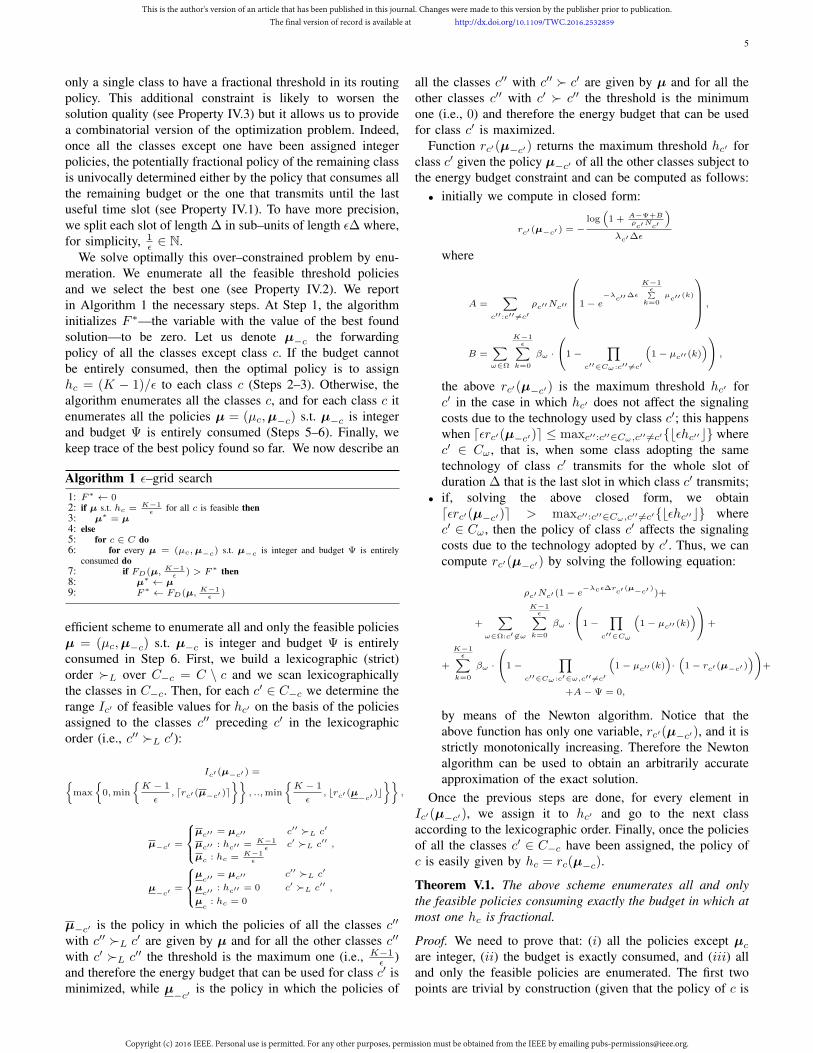
only a single class to have a fractional threshold in its routingpolicy. This additional constraint is likely to worsen thesolution quality (see Property IV.3) but it allows us to providea combinatorial version of the optimization problem. Indeed,once all the classes except one have been assigned integerpolicies, the potentially fractional policy of the remaining classis univocally determined either by the policy that consumes allthe remaining budget or the one that transmits until the lastuseful time slot (see Property IV.1). To have more precision,we split each slot of length ∆ in sub–units of length ε∆ where,for simplicity, 1

ε ∈ N.We solve optimally this over–constrained problem by enu-

meration. We enumerate all the feasible threshold policiesand we select the best one (see Property IV.2). We reportin Algorithm 1 the necessary steps. At Step 1, the algorithminitializes F ∗—the variable with the value of the best foundsolution—to be zero. Let us denote µ−c the forwardingpolicy of all the classes except class c. If the budget cannotbe entirely consumed, then the optimal policy is to assignhc = (K − 1)/ε to each class c (Steps 2–3). Otherwise, thealgorithm enumerates all the classes c, and for each class c itenumerates all the policies µ = (µc,µ−c) s.t. µ−c is integerand budget Ψ is entirely consumed (Steps 5–6). Finally, wekeep trace of the best policy found so far. We now describe an

Algorithm 1 ε–grid search1: F∗ ← 02: if µ s.t. hc = K−1

ε for all c is feasible then3: µ∗ = µ4: else5: for c ∈ C do6: for every µ = (µc,µ−c) s.t. µ−c is integer and budget Ψ is entirely

consumed do7: if FD(µ, K−1

ε ) > F∗ then8: µ∗ ← µ9: F∗ ← FD(µ, K−1

ε )

efficient scheme to enumerate all and only the feasible policiesµ = (µc,µ−c) s.t. µ−c is integer and budget Ψ is entirelyconsumed in Step 6. First, we build a lexicographic (strict)order L over C−c = C \ c and we scan lexicographicallythe classes in C−c. Then, for each c′ ∈ C−c we determine therange Ic′ of feasible values for hc′ on the basis of the policiesassigned to the classes c′′ preceding c′ in the lexicographicorder (i.e., c′′ L c′):

Ic′ (µ−c′ ) =max

0,min

K − 1

ε, drc′ (µ−c′ )e

, ..,min

K − 1

ε, brc′ (µ−c′ )c

,

µ−c′ =

µc′′ = µc′′ c′′ L c′

µc′′ : hc′′ = K−1ε c′ L c′′

µc : hc = K−1ε

,

µ−c′

=

µc′′

= µc′′ c′′ L c′

µc′′

: hc′′ = 0 c′ L c′′

µc

: hc = 0

,

µ−c′ is the policy in which the policies of all the classes c′′

with c′′ L c′ are given by µ and for all the other classes c′′

with c′ L c′′ the threshold is the maximum one (i.e., K−1ε )

and therefore the energy budget that can be used for class c′ isminimized, while µ−c′ is the policy in which the policies of

all the classes c′′ with c′′ c′ are given by µ and for all theother classes c′′ with c′ c′′ the threshold is the minimumone (i.e., 0) and therefore the energy budget that can be usedfor class c′ is maximized.

Function rc′(µ−c′) returns the maximum threshold hc′ forclass c′ given the policy µ−c′ of all the other classes subject tothe energy budget constraint and can be computed as follows:• initially we compute in closed form:

rc′ (µ−c′ ) = −log(

1 + A−Ψ+Bρc′Nc′

)λc′∆ε

where

A =∑

c′′:c′′ 6=c′ρc′′Nc′′

1− e−λ

c′′∆ε

K−1ε∑

k=0µc′′ (k)

,

B =∑ω∈Ω

K−1ε∑

k=0

βω ·

1−∏

c′′∈Cω :c′′ 6=c′

(1− µc′′ (k)

) ,

the above rc′(µ−c′) is the maximum threshold hc′ forc′ in the case in which hc′ does not affect the signalingcosts due to the technology used by class c′; this happenswhen dεrc′(µ−c′)e ≤ maxc′′:c′′∈Cω,c′′ 6=c′bεhc′′c wherec′ ∈ Cω , that is, when some class adopting the sametechnology of class c′ transmits for the whole slot ofduration ∆ that is the last slot in which class c′ transmits;

• if, solving the above closed form, we obtaindεrc′(µ−c′)e > maxc′′:c′′∈Cω,c′′ 6=c′bεhc′′c wherec′ ∈ Cω , then the policy of class c′ affects the signalingcosts due to the technology adopted by c′. Thus, we cancompute rc′(µ−c′) by solving the following equation:

ρc′Nc′ (1− e−λcε∆rc′ (µ−c′ ))+

+∑

ω∈Ω:c′ 6∈ω

K−1ε∑

k=0

βω ·

1−∏

c′′∈Cω

(1− µc′′ (k)

)+

+

K−1ε∑

k=0

βω ·

1−∏

c′′∈Cω :c′∈ω,c′′ 6=c′

(1− µc′′ (k)

)·(

1− rc′ (µ−c′ )))

+

+A−Ψ = 0,

by means of the Newton algorithm. Notice that theabove function has only one variable, rc′(µ−c′), and it isstrictly monotonically increasing. Therefore the Newtonalgorithm can be used to obtain an arbitrarily accurateapproximation of the exact solution.

Once the previous steps are done, for every element inIc′(µ−c′), we assign it to hc′ and go to the next classaccording to the lexicographic order. Finally, once the policiesof all the classes c′ ∈ C−c have been assigned, the policy ofc is easily given by hc = rc(µ−c).

Theorem V.1. The above scheme enumerates all and onlythe feasible policies consuming exactly the budget in which atmost one hc is fractional.

Proof. We need to prove that: (i) all the policies except µcare integer, (ii) the budget is exactly consumed, and (iii) alland only the feasible policies are enumerated. The first twopoints are trivial by construction (given that the policy of c is



6

the only potentially non–integer and is computed as the policythat consumes the budget given the policies of all the otherclasses). To prove the third point, we observe that I is always awell–defined range. Indeed, brc′(µ−c′)c returns the largest hc′that consumes exactly the remaining budget given the budgetconsumed by all the classes preceding c′ in the lexicographicorder. Assigning a policy larger than min

K−1ε , brc′(µ−c′)c

violates the budget constraint or violates the deadline τ . Ifthe policies assigned to the previous classes are feasible,then brc′(µ−c′)c is always non–negative. As well, brc′(µ−c′)creturns the smallest hc′ that consumes exactly the remainingbudget given the budget consumed by all the classes precedingc′ in the lexicographic order and assuming that the classesthat succeed transmit all the slots. Assigning a policy smallerthan max

0,minK−1

ε , drc′(µ−c′)e

does not allow one toconsume entirely the budget. Thus, by construction, for eachpolicy assigned to class c′ belonging to I , it is always possibleto find a feasible policy for the succeeding classes.

The number of policies enumerated by Algorithm 1 isexponential in C, being O((K−1

ε )|C|−1). We state the fol-lowing result on the optimality loss of the solution found byAlgorithm 1.

Theorem V.2. Let FD be the value of the solution returnedby Algorithm 1 and F ∗D the value of the optimal solution, thenwe have

FD

F∗D≥

1− ( 12 )K−1ε

1− ( 12 )|C|

K−1ε

.

Proof. Call µ∗ the optimal policy profile and call µc thepolicy profile in which hc′ = bh∗c′c for all c′ 6= c andhc = h∗c . Obviously, F ∗D ≥ FD(µc,

K−1ε ) and F ∗D ≥ FD ≥

maxcFD(µc,K−1ε ). This is because µc is a feasible policy

profile in which at most one policy is fractional that is notassured to consume exactly the budget. We can write a lowerbound for FD

(µc,

K−1ε

)as:

FD

(µc,

K − 1

ε

)=

= 1−∏c′∈C

K−1ε∏

k=0

X∗c′,k(λc′ ε∆, µc) ≥ 1−

K−1ε∏

k=0

X∗c,k(λcε∆, µc)

By using such lower bound over FD(µc,

K−1ε

), we can write:

FD

F∗D≥ max

c

1−∏K−1

εk=0 X∗c,k(λcε∆,µ

∗)

1−∏c′∈C

∏K−1ε

k=0 X∗c′,k(λc′ ε∆,µ

∗)

since, given µc and µ∗, we have hc = h∗c . Thus, we areinterested in:

min maxc

1−∏K−1

εk=0 X∗c,k(λcε∆,µ

∗)

1−∏c′∈C

∏K−1ε

k=0 X∗c′,k(λc′ ε∆,µ

∗)

where the minimization is over all the parameters. Althoughthe definition of X∗ is intricate, a bound can be derived disre-garding the exponential nature of all the X∗ and consideringthem as arbitrary values in [0, 1]. In this case, for reasonsof symmetry, the values that minimize the maximum ratio

prescribe X∗c,k = 12 for all c. This leads to the bound stated

in the theorem.

Notice that the theoretical lower bound does not depend onwhether the signaling costs are present. The worst case is whenK = 2 and |C| → ∞, obtaining a ratio of 1− 1

2

1ε . However,

it can be observed that the worst case ratio goes to oneexponentially in 1

ε . Thus we can obtain a good approximationratio with a small value of 1

ε , e.g., the theoretical lower boundover the approximation ratio is about 1− 10−4 when 1

ε = 10.Algorithm 1 is an approximation scheme (AS), given that theratio goes to one as ε goes to zero.

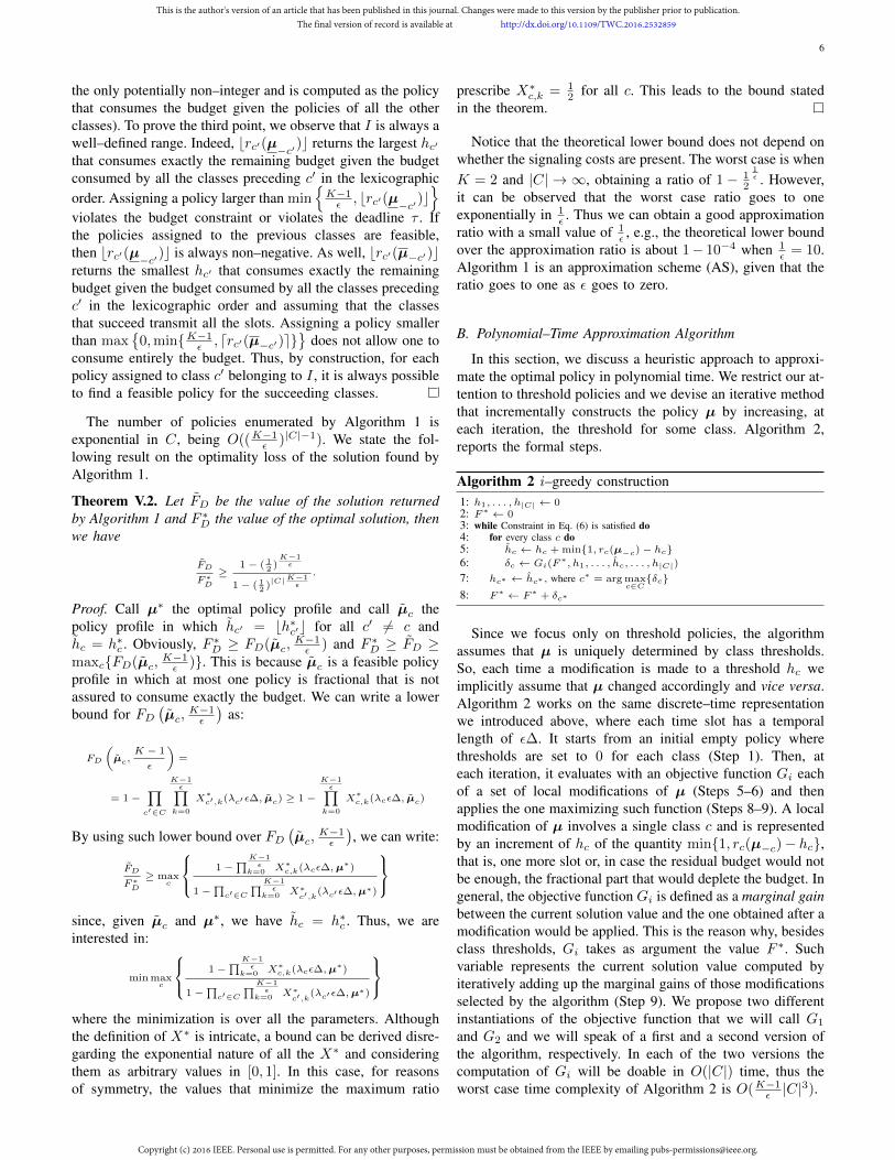
B. Polynomial–Time Approximation Algorithm

In this section, we discuss a heuristic approach to approxi-mate the optimal policy in polynomial time. We restrict our at-tention to threshold policies and we devise an iterative methodthat incrementally constructs the policy µ by increasing, ateach iteration, the threshold for some class. Algorithm 2,reports the formal steps.

Algorithm 2 i–greedy construction1: h1, . . . , h|C| ← 02: F∗ ← 03: while Constraint in Eq. (6) is satisfied do4: for every class c do5: hc ← hc + min1, rc(µ−c)− hc6: δc ← Gi(F

∗, h1, . . . , hc, . . . , h|C|)

7: hc∗ ← hc∗ , where c∗ = arg maxc∈Cδc

8: F∗ ← F∗ + δc∗

Since we focus only on threshold policies, the algorithmassumes that µ is uniquely determined by class thresholds.So, each time a modification is made to a threshold hc weimplicitly assume that µ changed accordingly and vice versa.Algorithm 2 works on the same discrete–time representationwe introduced above, where each time slot has a temporallength of ε∆. It starts from an initial empty policy wherethresholds are set to 0 for each class (Step 1). Then, ateach iteration, it evaluates with an objective function Gi eachof a set of local modifications of µ (Steps 5–6) and thenapplies the one maximizing such function (Steps 8–9). A localmodification of µ involves a single class c and is representedby an increment of hc of the quantity min1, rc(µ−c)− hc,that is, one more slot or, in case the residual budget would notbe enough, the fractional part that would deplete the budget. Ingeneral, the objective function Gi is defined as a marginal gainbetween the current solution value and the one obtained after amodification would be applied. This is the reason why, besidesclass thresholds, Gi takes as argument the value F ∗. Suchvariable represents the current solution value computed byiteratively adding up the marginal gains of those modificationsselected by the algorithm (Step 9). We propose two differentinstantiations of the objective function that we will call G1

and G2 and we will speak of a first and a second version ofthe algorithm, respectively. In each of the two versions thecomputation of Gi will be doable in O(|C|) time, thus theworst case time complexity of Algorithm 2 is O(K−1

ε |C|3).



7

First Version, Locally Optimizing FD: In the first version ofAlgorithm 2, we define G1 in order to obtain the maximizationof the marginal gain of FD, i.e., the delivery probability.Formally, we have that at Step 6 it holds that Gi = G1 whereG1(F ∗, h1, . . . , h|C|) = FD(µ, (K − 1)/ε)−F ∗. (Recall thatµ is assumed to be the unique policy obtained from thresholdsh1, . . . , h|C|). Under such definition, δc represents the benefit,in terms of delivery probability, that an additional (integer orfractional) time slot for class c would introduce at the currentiteration. By exploiting a result presented in [29] we are ableto provide a bound on the solution quality obtained with thisversion of the greedy algorithm. The result we will exploit canbe formalized as follows (see [29] for a complete derivation).

Theorem V.3 (From [29]). Given a ground set Θ, a set func-tion Φ : 2Θ → R, and a positive integer W ∈ N+, let us con-sider the problem of finding S∗ = arg maxS⊆Θ,|S|≤W Φ(S).Then if Φ is submodular, we have that for every integer0 ≤ l ≤ W , Φ(Sl) ≥ (1 − e−l/W )Φ(S∗), where Sl ∈ Θ isthe set built after l iterations of the following greedy element–selection rule

Si =

∅ if i=0Si−1 ∪ arg maxs∈Θ Φ(Si−1 ∪ s) else

(7)

Theorem V.3 states that greedily maximizing a submodularset function introduces a bounded suboptimality. Eventually,the bound converges to (1 − 1

e ) (≈ 0.63) when l = W , thatis, when the maximum number of selections allowed by thecardinality constraint is made.

In order to apply the above result to Algorithm 2, we need toshow that the problem of finding an optimal integer policy canbe expressed as the maximization of a submodular set functionsubject to a cardinality constraint. This similarity can be shownby mapping our problem to the following set–based formalinterpretation. Let us assume that each element in the groundset θ ∈ Θ is a pair (c, k) where c ∈ C and k ∈ 1, . . . , K−1

ε .That is, each element of S prescribes that a specific classtransmits in a specific slot. Then, every subset S ⊆ Θ can beuniquely associated with an integer (not necessarily threshold–based) policy µS . Indeed, a unique correspondence betweenS and µS can be obtained by the following construction rule:

µSc (k) =

1 (c, k) ∈ S0 else

Therefore, the objective function for a policy µS can berewritten as a set function by operating the following simpleassignment: Φ(S) = FD(µS , (K − 1)/ε).

The second necessary step is to derive a cardinality con-straint to define the problem’s feasibility region. In our prob-lem, the feasibility of a policy is determined by the budgetlimit, namely by the constraint in Eq. 6. For this reason, ideallyone would like to find a W such that |S| > W if and only ifµS violates the constraint in Eq. 6. However, it can be easilyshown that budget feasibility cannot be directly expressed witha cardinality constraint. The reason is straightforward. Thebudget of a policy does not solely depend on the number oftransmitting slots, but also on how those slots are distributedamong the different classes. Nevertheless, a necessary (not

sufficient) cardinality upper bound can be determined via thefollowing theorem.

Theorem V.4. Any feasible threshold integer policy cannotassign full probability of transmission to more than W =minmaxcrc(µ∅), K−1

ε , where µ∅ is the empty policy.

Proof. Let us assume that c = arg maxcrc(µ∅). Then,consider a threshold policy µS where |S| > W . If µS isbudget–feasible then, by definition, the policy obtained in thisway should be feasible too: for every (c, k) ∈ S where c 6= csubstitute (c, k) with (c, hc+1). However, by definition of Wsuch a policy cannot be budget–feasible.

Under the above assumption, the optimal integer policyproblem can be associated, up to a relaxation of the feasibilityconstraint, with the maximization of the set function Φ(S),subject to |S| ≤ W . By relaxing the cardinality constraintwe can still derive an approximation bound even though wecannot guarantee its tightness. In the next step we show FDsubmodularity.

Property V.5. The set function Φ is submodular w.r.t. Θ.

Proof. First, let us consider a setting with a single class. FromProperty IV.2, we can focus only on threshold policies andrewrite Φ as a function of h, namely the threshold value (thisvalue, in general, can be non–integer). Then it can be easilyshown that Φ(h) is a concave function since the Hessianmatrix has strictly negative eigenvalues. Given a functionf : N → R+, then f(|S|) is submodular on the subsets Sof an arbitrary set Ω if and only if f is concave [30]. We canthen conclude that Φ is submodular in the case of a singleclass. Let us now show submodularity for the case with twoclasses. Let us denoted with ∆Φ(S|e) the marginal gain ofΦ obtained by adding the element e to the set S, namelyadding a transmitting slot to some class to the policy µS . Forsubmodularity to hold, we need to show that for every Sa,Sb, e such that Sa ⊆ Sb ⊂ Ω and e ∈ Ω \ Sb we havethat ∆Φ(Sa|e) ≥ ∆Φ(Sb|e). By definition e adds a slot toa single class, let us assume without loss of generality thatthis class is c1. Also, let us denote with Φci our functioncomputed as if ci was the only present class. Then we have∆Φ(Sa|e) = [1−(1−(Φc1(S)+∆Φc1(Sa|e)))(1−Φc2(S))]−[1− (1−Φc1(S))(1−Φc2(S))] = (1−Φc2(Sa))∆Φc1(Sa|e)and, analogously, ∆Φ(Sb|e) = (1 − Φc2(Sb))∆Φc1(Sb|e).Since ∆Φc1(Sa|e) ≥ ∆Φc1(Sb|e) by submodularity of Φc1and Φc2(Sb) ≥ Φc2(Sa) by Φc2 monotonicity, we have thatΦ is submodular. The same reasoning can be extended to anarbitrary number of classes.

Theorem V.3 can be applied by showing that Algorithm 2corresponds to the greedy element–selection rule reported inEq. 7. The rule of Eq. 7, when applied to the integer policyproblem, proceeds by locally optimal appends in the same waythat Algorithm 2 does. Hence, we have:

Theorem V.6. Let us denote with S∗ the policy returned byAlgorithm 1 and with S1

l the policy constructed by Algorithm 2(version 1) after l iterations. We then have that FD(S1

l ,K) ≥(1− e−l/W )FD(K,S∗).



8

Proof. The inequality stated in the theorem follows imme-diately from the following two properties. First, by apply-ing Theorem V.3 to Algorithm 2 (version 1) we have thatFD(S1

l ,K) ≥ (1 − e−l/W )FD(S∗,K). Second, since S∗ isthe optimal solution of a relaxed version of the integer policyproblem, it holds that FD(S∗,K) ≤ FD(S∗,K) .

The previous theorem, provides an online bound on thesolution quality, being it dependent on the number of iterationsthe algorithm will succeed in performing without violating theactual budget constraint. An offline guarantee can be given bycomputing the minimum number of slot sc to be assignedto each class c. This number can be computed by settingµc′(i) = 1 ∀i 0 ≤ i ≤ K, c′ 6= c and computing the maximumnumber of time slots during which c can transmit withoutsaturating the budget.

Corollary V.7. For any solution S1 obtained with Algorithm 2(version 1) we have that:

FD(S1, K) ≥

(1− e

−∑c∈C

sc/W)FD(S

∗, K).

Second Version, Normalizing G1 with Budget Costs: Thesecond version of our algorithm adopts objective function G2,obtained by normalizing G1 with the budget cost that a localmodification (the additional time slot) would introduce. Asa consequence, given a local modification of µ as definedabove, here δc represents a ratio between the marginal gain inthe delivery probability obtained if applying such modificationand the additional transmission costs that would be paid. Forsimplicity, we do not consider signaling costs, also because ex-tending our approximate analysis by including them does notseem straightforward. Under the assumption that no signalingcosts are present and that we deal with threshold policies, eachtransmission has an independent cost and the budget spent by apolicy S is given by ψ(S) =

∑(c,k)∈S

ρcNce−λc∆(k−1)(1−e−λc∆)and,

consequently, G2(µ) =G1(µ)

ψ((c,hc+1)) .If we modify the rule in Eq. 7 by normalizing the objective

function by the budget cost for each candidate element, wecan again show the equivalence between the new rule andAlgorithm 2 (version 2). As a consequence, we can againresort to a result presented in [29] and provide a qualitybound on the solution obtained with the combination of thetwo versions of Algorithm 2 when signaling costs are notconsidered.Theorem V.8. If no signaling costs are present, then it holdsthat

maxFD(S1, K), FD(S

2, K) ≥

1

2(1−

1

e) maxS⊆Θ:ψ(S)≤Ψ

FD(S,K)

Proof. The proof follows immediately by the considerationmade above and a straightforward adaptation of results pre-sented in [29].

VI. EXTENSION TO MULTI–HOP ROUTING

We initially describe how the formulation of the problemchanges in the case of `–hop routing with ` ≥ 3. At first, weneed some assumptions about the functioning of the routingprotocol. More precisely, we assume that: during a time slot,

if a mobile node contacts both the source and other mobilenodes carrying the packet, then the mobile node receives thepacket directly from the source, and, if a mobile node hasreceived a packet from another mobile node before contactingthe source, then the mobile node does not receive the packetalso from the source. Furthermore, as assumed in the caseof two–hop routing, if a mobile node has dropped a packet, itwill never get the packet again in future. With multiple classes,we have two different scenarios: the one in which a node ofclass c cannot transmit the packet to a node of class c′ withc 6= c′ and the one in which it can do. Our aim is to find thebest (approximate) transmission policy of the source, giventhe transmission policies of the mobile nodes (characterizedby time–out tc).

We focus on the extension of Algorithm 2 (although also theextension of Algorithm 1 is possible, it requires long calcula-tions and it is less significant requiring exponential time). Theextension can be simply obtained by providing a procedureto calculate Xc,k necessary to compute objective function Fand a procedure to calculate the cost of a transmission policy.Indeed, the proof of submodularity and the bounds derived inSection V-B hold also with `–hop routing.

We focus on the calculation of Xc,k. We initially describehow, in the basic case of two–hop routing without time–out tc,variable Xc,k can be computed. This is useful for presentingthe general case. We denote by Xc,k(i,µ) the probability that,given µ, at slot k there are i nodes of class c directly infectedby the source. The term Xc,k(i,µ) can be computed as:

Xc,k(i,µ) =i∑

h=0

Xc,k−1(h,µ) (1−Qc,k−1,k(µ))i−h

(Qc,k−1,k(µ))n−h

(Nc − hi− h

)

It can be observed that the computation of Xc,k(i,µ) requirestime and space O(|C|NcK).

We show now how, in the case of two–hop routing withtime–out tc, variables Xc,k and Yc,k can be computed.With abuse of notation, we denote by Xc,k(i,µ|n) the termXc,k(i,µ) when the number of mobile nodes is n, potentiallydifferent from Nc. We have:

Yc,k(i,µ) =

Xc,k(i,µ|Nc) k ≤ tcNc−i∑j=0

Xc,k−tc (j,µ|Nc)Xc,tc (i,µ|Nc − j) tc < k

It can be observed that the computation of Yc,k(i,µ) requiresthe computation of Xc,k(i,µ|n) for any n ∈ 1, . . . , Nc, andtherefore it requires time and space O(|C|(Nc)2K).

Now we focus on the case with `–hop routing. For thesake of clarity, we present the case with only one class andwithout time–out tc, the extension to the general case isdiscussed below. Initially, denote by Zk(i1, i2, . . . , i`−1,µ) theprobability that, given µ, at slot k there are i1 nodes with a1–hop infection, i2 nodes with a two–hop infection, and soon. Variable Zk is defined in Eq. (8).

It can be observed that computing Zk(i1, i2, . . . , i`−1,µ)requires time and space O((Nc)

`K). The exponential size in` cannot be circumvented, being necessary to keep trace of allthe possible configurations of mobile nodes at different hopsthat are exponential in `. Then, Xk(i,µ) is:



9

Zk(i1, i2, . . . , i`−1,µ) =

i1∑h1=0

i2∑h2=0

..

i`−1∑h`−1=0

Zk−1(h1, h2, . . . , h`−1,µ) · (1−Qk−1,k(µ))i1−h1 (Qk−1,k(µ))

n−i1−∑`−1j=2

hj(Nc − i1 −∑`−1

j=2 hj

i1 − h1

)

·∏w=2

(1−

(Q

mobk−1,k

)hw−1)iw−hw (

Qmobk−1,k

)Nc−∑wv=1 iv(Nc −∑w−1

v=1 iv −∑`−1v=w hv

iw − hw

)(8)

Xk(i,µ) =

i∑i1=0

i−i1∑i2=0

· · ·i−∑`−3w=1 iv∑

i`−2=0

Zk

i1, i2, . . . , i`−2, i−`−2∑w=1

iv,µ

where Qmob

k−1,k is the probability that two mobile nodes do nothave any contact between slots k − 1 and k. In case of `–hop routing with |C| classes without time–out tc we need astructure Zc,k(i1, i2, . . . , i`−1,µ) of size O(|C|(Nc)`K) if anode of class c cannot transmit to a node of class c′ withc 6= c′, whereas we need a structure Zc,k(i1,1, . . . , i|C|,`−1,µ)of size O(n|C|`K) if a node of a given class c can transmitthe packet to nodes of different classes than c. Finally, whenmobile nodes have a time–out tc, it is necessary an extramultiplicative cost of O(

∑cNc).

Finally, we now focus on the energy cost of a transmissionpolicy. The energy cost depends only on the number of mobilenodes directly infected by the source. That is:

ρc

i∑i1=0

i1

i−i1∑i2=0

· · ·i−∑`−3w=1 iv∑

i`−2=0

Zk

i1, i2, . . . , i`−2, i−`−2∑w=1

iv,µ

.

The extension of Algorithm 2 to ` hops is then easy andinvolves only Steps 5 and 6. Informally, these steps aresubstituted as follows: given a class c, hc is increased by 1 andboth FD and the energy cost are computed as described above.If the remaining budget is smaller than the cost of increasinghc by 1, then hc is reduced to satisfy the budget by employingthe Newton algorithm. Finally, values δc and hc are returned.

VII. PERFORMANCE EVALUATION

A. Evaluation Setting

We generated instances by considering the discretized pa-rameter space of Tab. II. The reference scenario is an urbanarea populated by mobile devices carried by pedestrians,bicycles, vehicles equipped with heterogeneous transmissiontechnologies (ZigBee, Bluetooth 4.0. and WiFi Direct). Wederive the values for ρ and β by considering the technicalspecifications of each technology and assuming an applicationscenario with a 5kB packet and ∆ = 10s. For simplicity, weassign the same number of users to each class.

Unless differently specified, we consider up to 3 classesand a discretization ε ∈ 1, 1/3, 1/5. This represents a goodtradeoff between accuracy and computational effort to evaluateour algorithms as shown, see Fig. 1, by the theoretical lowerbound of the delivery probability (Theorem V.2) for differentresolutions and numbers of classes. As it can be seen, amaximum resolution of ε = 1/5 is a reasonable choice toguarantee about 95% of the optimal solution quality withoutthe burden of a prohibitive number of time slots. On the other

TABLE II: Parameters used for experiments.Deliverydeadline(τ/∆)

25, 50, 100, 250 time units

Networkradius(L)

350, 500, 750, 1000m

Numberof nodes(Nc)

9, 15, 20

Mobilityprofiles(vc)

pedestrians (1.5m/s),bicycles (6m/s),vehicles (9m/s)

TechnologyZigBee (ρ = 0.1989J , β = 0.7204× 10−5J , R = 15m)Bluetooth 4.0 (ρ = 0.1278J , β = 0.1136× 10−5J , R = 50m)WiFi Direct (ρ = 0.0642J , β = 0.0392× 10−5J , R = 100m)

side, by adopting a maximum number of 3 classes we obtaina case which is fairly close to the worst case (derived for aninfinite number of classes) and that is computable by meansof our grid algorithm (recall that our grid search requires acomputing time exponential in the number of classes).

0 2 4 6 8 100.5

0.6

0.7

0.8

0.9

1

1/ε

Bo

un

d v

alu

e

0 5 10 15 20

0.75

0.8

0.85

0.9

0.95

1

Number of Classes

Bo

und v

alu

e

Bound value

Worst case

Fig. 1: Theoretical lower bound over solution’s quality (The-orem V.2).

We use the following benchmarks for evaluating our algo-rithms in two–hop routing scenarios.

1) Greedy on Arrival Rate: it sorts the classes in descend-ing order of λc, then it allocates all the possible budget tothe classes from the first one to the last one. The rationale isthat we expect that the larger the arrival rate the larger thedelivery probability. The complexity of this algorithm is low:the policy can be found by solving at most |C| equations.

2) Class–Independent Policies: it searches for the optimalsolution of an over–constrained problem in which the policiesrelated to all the classes are the same, formally µ(k) = µc(k)for all c, and, when the policy is probabilistic, then either thesource transmits to all the classes or it does not transmit atall. This leads to a new formulation of the budget constraint:

∑c∈C

ρcNc ·(1−Qc,0,K(µ))+∑ω∈Ω

K−1∑k=0

βω(

1− (1− µ(k))|Cω|

)≤ Ψ



10

By Property IV.1, the optimal policy is such that the bud-get Ψ is completely consumed and therefore the aboveinequality holds with equality. Therefore, the optimizationproblem reduces to the problem of finding the policy thatcompletely consumes the budget. Formally, interpreting the(class–independent) threshold h as a continuous variable, wecan write:

g(h) =∑c∈C

ρcNc · (1− e−λc∆h)+

∑ω∈Ω

βωbhc+∑ω∈Ω

βω(

1− (1− h+ bhc)|Cω|)−Ψ = 0

Function g is a single–variable function strictly monotonicallydecreasing in h and infinitely differentiable. Such a functionadmits only one zero, and therefore the above equation admitsonly one solution. Such a solution can be found (approxi-mately) by using the Newton method that, due to the functionproperty holding in this case, has a quadratic convergencespeed (the number of correct digits roughly doubles in everyiteration). Thus, we obtain an approximate solution of highquality within very short time.

3) Upper Bound over the Optimal Value: an upper boundover the value of the optimal solution can be found by usinga variation of the algorithm described in Section V-A. Moreprecisely, we use Algorithm 1 to enumerate all the policiesconsuming entirely the budget and we change each policyrounding each hc to the smallest integer and then adding1 for every c. Notice that these new policies violate thebudget constraint. Among all these policies we find the onemaximizing the delivery probability. Its value is an upperbound over the value of the optimal policy. In the following,we denote this value as UB. The proof sketch follows. Callµ∗ the optimal policy profile with (potentially fractional)thresholds h∗c . Call µ a generic policy profile obtained asdescribed above. It can be easily observed (it follows fromthe fact that, fixed the policies of all the classes but one, thepolicy of the remaining class that consumes entirely the budgetis always one) that there alway exists a policy profile µ suchthat hc ≥ h∗c for all c. Therefore, given that the objectivefunction is strictly monotone in hc, the objective value of µis strictly better than the value µ∗.

4) Fluid Approximation: We use the approach describedin [2] based on fluid approximation to derive approximaterouting policies.

B. Comparing l–hops Routing Policies

We apply our greedy algorithms when the number of hops isin 1, 2, 3, 4, 5, epidemic to the simulation setting describedabove restricting the number of classes to be one. In this case,our algorithms return optimal solutions. We evaluate how thedelivery probability and the ratio between delivery probabilityand the number of expected transmissions in the networkvary as the number of hops varies. The first index provides ameasure of the improvement of the objective function, whilethe second index provides a measure of efficiency betweenobjective function and consumed energy. In all our simula-tions, we observed that the delivery probability increases in the

number of hops and the increment decreases exponentially inthe number of hops, achieving asymptotically the epidemicrouting, while the ratio between delivery probability andexpected number of transmissions decreases in the numberof hops. We report the data of the most significant simulationin Fig. 2, in which we use WiFi Direct, bicycles, L = 500m,K = 25 and a variable number of nodes. This shows thattwo–hop routing provides the best tradeoff between deliveryprobability and energy consumption, with a ratio of almost5 w.r.t. the epidemic routing and a ratio of about 2 w.r.t.three–hop routing. From here on, we focus our performanceevaluation on two–hop routing protocol.

1 5 10 13 15 18 200

0.1

0.2

0.3

0.4

0.5

0.6

0.7

0.8

0.9

1

Number of Nodes

FD

2 Hops

3 Hops

4 Hops

5 Hops

Epidemic

1 5 10 13 15 18 200.04

0.06

0.08

0.1

0.12

0.14

0.16

0.18

0.2

0.22

Number of Nodes

FD /

E[in

fecte

d n

od

es]

2 Hops

3 Hops

4 Hops

5 Hops

Epidemic

Fig. 2: Performance at different hops of Greedy construction(1). At left: delivery probability. At right: delivery probabilitydivided by expected number of transmissions in the network.C. Algorithms Performance Analysis with two hops

Fig. 3 reports how FD/UB varies as the values of theparameters τ, L,Nc vary as summarized in Table II, |C| ∈1, 2, 3, and 1

ε = 5. For each parameter, we average FD/UBover the other instances sharing the same value for thatparameter. It can be observed that grid search and greedyconstructions obtain a remarkably better performance in eachcase when compared with the benchmarking greedy algorithmsbased on the arrival rate and the class–independent one. Notexploiting the knowledge about the different classes and solelyconsidering the arrival rate turned out to achieve very similarperformances. By increasing the value of τ , it can be seenhow this gap with the benchmarks shrinks, suggesting theintuition that when the deadline for packet delivery is largeeven simplistic policies are able to obtain good delivery prob-abilities. Another aspect that can be observed is that greedyconstructions revealed to be quite effective for the tested cases,since they were able to obtain high performances comparableto the grid search. By increasing the value of L, it can beseen how this gap with the benchmarks increases, insteadthe gap keeps to be approximately constant as Nc and |C|vary. Interestingly, the approximation ratio of our algorithmsis almost constant (i.e., > 99%) w.r.t. all the parameters values.

A more detailed overview on how the performance (mea-sured again as FD/UB) varies with ε at different values ofτ is shown by the boxplots of Fig. 4. These graphs showthe similarity in performance between the grid search andthe greedy constructions algorithms. These last ones obtainedworse performances for a limited number of outlier instances.Also it is evident how having finer resolutions remarkablyimproves the solution quality. As shown by the boxplots, thelevels of statistical significance corroborate our claims.

The above results suggest that greedy constructions seemto be quite effective approaches to approximate the optimal



11

25 50 100 2500.7

0.8

0.9

1

τ / ∆

Ave

rag

e F

/UB

Grid search

Greedy construction (1)


Greedy (arrival rate)

Class−independent

350 500 750 10000.7

0.8

0.9

1

L

Ave

rag

e F

/UB

9 15 200.7

0.8

0.9

1

Number of Nodes

Ave

rag

e F

/UB

1 2 30.7

0.8

0.9

1

Number of Classes

Ave

rag

e F

/UB

Fig. 3: Average FD/UB w.r.t. different parameters at 1ε = 5.

1 1/3 1/5

0.7

0.8

0.9

1

ε

Grid search

τ /

∆=

25

1 1/3 1/5

0.7

0.8

0.9

1

ε


1 1/3 1/5

0.7

0.8

0.9

1

ε


1 1/3 1/5

0.7

0.8

0.9

1

ε

Grid search

τ /

∆=

50

1 1/3 1/5

0.7

0.8

0.9

1

ε


1 1/3 1/5

0.7

0.8

0.9

1

ε


1 1/3 1/5

0.7

0.8

0.9

1

ε

Grid search

τ /

∆=

10

0

1 1/3 1/5

0.7

0.8

0.9

1

ε


1 1/3 1/5

0.7

0.8

0.9

1

ε


1 1/3 1/5

0.7

0.8

0.9

1

ε

Grid search

τ /

∆=

25

0

1 1/3 1/5

0.7

0.8

0.9

1

ε


1 1/3 1/5

0.7

0.8

0.9

1

ε


Fig. 4: Boxplots showing FD/UB w.r.t. τ for different algorithms.

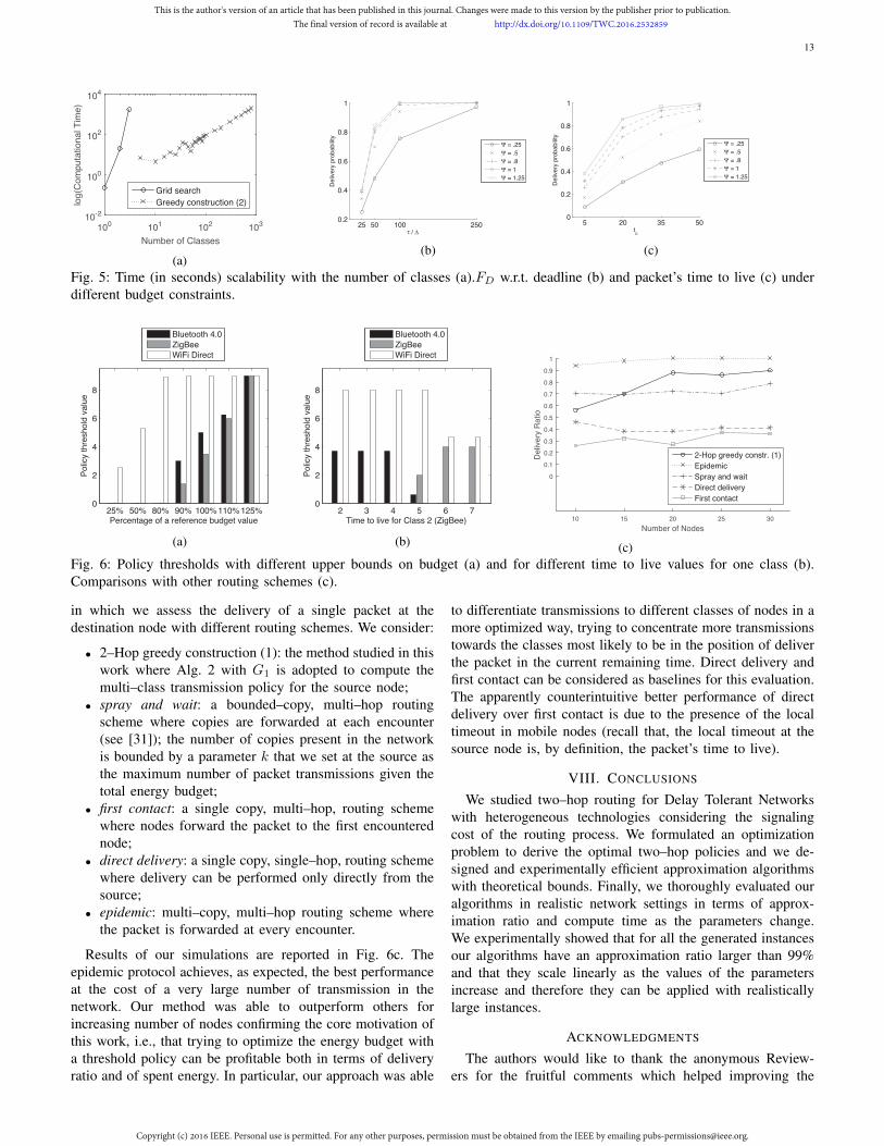
policy requiring, at the same time, much lower computationaleffort than the grid search. In Fig. 5a, we show a com-parison between computational times obtained with the gridsearch and the greedy construction algorithms respectively.In particular, we evaluated the algorithms’ scalability whenthe number of classes grows. To obtain these results wefixed the values of some parameters (ε = 1/3, τ = 100,Nc = 10, L = 500) and we generated random mobilityprofiles and transmission technologies by uniformly samplingfrom the following intervals: Rc ∈ [15, 50], vc ∈ [1, 15],ρi ∈ [0.05, 0.25], βc ∈ [3 × 10−7, 8 × 10−7]. It is easy tosee how grid search shows an exponential growth in time,while greedy construction proved to be much more efficient

even for larger number of classes. Considering a deadline of 1hour, grid search was not able to compute a solution for morethan 4 classes, while greedy construction managed to computesolution up to 800 classes. Notice that the time needed onaverage to find the best policy (i.e., 10s with |C| ≤ 10 and100s with |C| ≤ 100) may be, in some scenarios, excessivelylong. Thus, to have a more accurate estimate of the overheadin real–world system, we implemented our approximationalgorithms in C language, obtaining a compression of about100 times (as observed in the literature for MATLAB vs. Cfor a number of applications). Such an overhead is compliantwith the most application of DTNs.

Finally, we evaluate the accuracy of the fluid approximation



12

approach. For each simulation setting described above, werun our approximation algorithms and the fluid approximationalgorithm and we compare the solutions in terms of averageFD. In our results, we excluded the basic settings with|C| = 1, in which the fluid approximation is optimal asour approximation algorithms. As in other applications, fluidapproximation provides an accurate approximation when thenumber of users/mobile nodes is large. More precisely, onaverage over the number of classes, the error (in percentage)of the fluid approximation w.r.t. our greedy algorithms behavesas 6.44 + 31.01 exp[−0.135

∑cNc] with a confidence bound

of 95%, providing thus an average error from about 35% forfew mobile nodes to about 5% for 100 mobile nodes. Thissuggests that with 100 mobile nodes or less our algorithms,besides introducing suitability for any number of hops, canprovide an important improvement w.r.t. the state of the art.

D. Two–Hop Routing Analysis

We now focus on how two–hop routing policies computedwith our most viable method (greedy constructions) behavew.r.t. absolute and relative temporal deadlines, that is τ andthe time to live tc for a particular class c. Indeed, togetherwith budget requirements, temporal deadlines turned out to bethe most sensible parameters, namely dimensions along whichperformance exposed remarkable variations.

Fig. 5b depicts how the delivery probability varies as τis set to increasing values for a number of budget settings.For such experiments we considered again three differentclasses (ZigBee, Bluetooth 4.0, and WiFi Direct associatedwith mobility profile in increasing speed as per Table II)with the same number of nodes (20), no packet discardingand the same relative budget scale we used in the previoussection. The trends confirm the intuition by suggesting thatstrict delivery deadlines are a critical factor in worsening theexpected performance of the computed policy. On the otherside, the influence exercised by the budget seems to muffle asits value becomes higher and higher.

In Fig. 5c we assess the impact of the packet’s time tolive on the delivery probability. In this experiment we usedthe same three classes as before but we enabled the packetdiscarding behavior setting a given tc equal for all the classes.We set τ/∆ = 50 in order to disable packet discarding whentc = 50. What can be observed from the figure is a trendsimilar to the one observed for the delivery deadline with thefollowing interesting difference. Here variations on the budgetconstraint seem to have a slightly stronger impact than before,suggesting that when nodes start to drop packets having extraunits of budget can introduce non–negligible improvements inthe performance.

Fig. 6a and 6b depict a qualitative evaluation of the policiesreturned by our algorithms. The same three classes as beforeare considered before and, for clarity, we selected an instancewhere τ/∆ = 10 (similar trends could be observed in anyother setting). In Fig. 6a, we consider a reference value forthe budget upper bound Ψ and we show how the thresholds ofthe optimal policy (obtained with grid search) are distributedacross the three different technologies. It can be observed how,

by increasing the budget, the optimal policy tends to scheduletransmissions with all the three technologies. When the budgetgets smaller and smaller, then the policy tries to rely more onthose technologies that have a longer communication range.

In Fig. 6b we show how policies change as different time tolive values are adopted. We set tc2 = 4 for the class adoptingBluetooth 4.0 technology and tc3 = 2 for that using WiFiDirect. The time to live for the class using ZigBee varies asshown in the picture. As it can be seen, such class is not evenexploited by the policy when its time to live is small, theother two classes are preferred. Interestingly, WiFi is assigneda higher threshold even though it has the lowest time to live(higher transmission range and node velocity provide somekind of overcompensation). As tc increases, ZigBee starts to beincluded in the classes used by the policy until it is completelypreferred over Bluetooth 4.0. Such trend demonstrates howthere are settings where less profitable classes (in terms ofspeed and transmission range) can be preferred over betterones due to a particular configuration of the time to live values.

E. Comparison with state of the art techniques

We complement the previous qualitative observations witha comparative analysis of our method against a number ofrouting schemes proposed in literature that operate underthe same assumption of no a priori mobility knowledge wetook in this work. We selected ONE (Opportunistic NetworkEnvironment simulator) [4] to run our simulations as it offersembedded support to simulate realistic wireless technologies,as well as built-in modules running state-of-the-art routingschemes. Since we are interested in comparing the proposedapproach against state-of-the-art alternatives, we focus hereon results obtained with a specific setting of the referencescenario parameters; even if the simulation results might ob-viously change in the absolute value if changing the simulationenvironment (i.e., considering different mobility models), theproposed simulation campaign is indeed insightful to showcasethe relative performances trends of the considered delay tol-erant routing techniques. In detail, we consider three differentclasses of nodes. For simplicity we assume that each classhas the same number of nodes and the same mobility profilewith average speed of 6m/s. Transmission technologies areZigBee, Buetooth 4.0, and WiFi Direct for each class respec-tively (see Table II for the associated parameters). The sourcenode energy budget is set by taking as a reference the batteryof a smartphone (approx. 5.45Wh) and by considering anapplication layer consuming no more than the 30% of the totalenergy with a daily maximum load of 20Mb of data. Assumingthat a single application packet has a size of 5kb we obtain abudget of 1.4715J for each packet delivery. Each packet has tobe delivered within 15 minutes from its creation at the sourceand each mobile node (excluding source and destination) hasa local timeout of 5 minutes. Nodes move randomly in afree environment of radius of 700m. We consider differentnumber of nodes N ∈ 10, 15, 20, 25, 30 (recall that eachclass has the same number of nodes so each experiment has3N + 2 total nodes populating the environment). For eachN we generate 100 different random joint mobility patterns



13

Number of Classes

100

101

102

103

log(C

om

puta

tional T

ime)

10-2

100

102

104

Grid search


(a)

25 50 100 2500.2

0.4

0.6

0.8

1

τ / ∆

De

live

ry p

rob

ab

ility

Ψ = .25

Ψ = .5

Ψ = .8

Ψ = 1

Ψ = 1.25

(b)

5 20 35 500

0.2

0.4

0.6

0.8

1

tc

De

live

ry p

rob

ab

ility

Ψ = .25

Ψ = .5

Ψ = .8

Ψ = 1

Ψ = 1.25

(c)

Fig. 5: Time (in seconds) scalability with the number of classes (a).FD w.r.t. deadline (b) and packet’s time to live (c) underdifferent budget constraints.

25% 50% 80% 90% 100%110% 125%0

2

4

6

8

Percentage of a reference budget value

Po

licy t

hre

sh

old

va

lue

Bluetooth 4.0

ZigBee

WiFi Direct

(a)

2 3 4 5 6 70

2

4

6

8

Time to live for Class 2 (ZigBee)

Po

licy t

hre

sh

old

va

lue

Bluetooth 4.0

ZigBee

WiFi Direct

(b)Number of Nodes

10 15 20 25 30

Deliv

ery

Ratio

0

0.1

0.2

0.3

0.4

0.5

0.6

0.7

0.8

0.9

1

2-Hop greedy constr. (1)

Epidemic

Spray and wait

Direct delivery

First contact

(c)Fig. 6: Policy thresholds with different upper bounds on budget (a) and for different time to live values for one class (b).Comparisons with other routing schemes (c).

in which we assess the delivery of a single packet at thedestination node with different routing schemes. We consider:

• 2–Hop greedy construction (1): the method studied in thiswork where Alg. 2 with G1 is adopted to compute themulti–class transmission policy for the source node;

• spray and wait: a bounded–copy, multi–hop routingscheme where copies are forwarded at each encounter(see [31]); the number of copies present in the networkis bounded by a parameter k that we set at the source asthe maximum number of packet transmissions given thetotal energy budget;

• first contact: a single copy, multi–hop, routing schemewhere nodes forward the packet to the first encounterednode;

• direct delivery: a single copy, single–hop, routing schemewhere delivery can be performed only directly from thesource;

• epidemic: multi–copy, multi–hop routing scheme wherethe packet is forwarded at every encounter.

Results of our simulations are reported in Fig. 6c. Theepidemic protocol achieves, as expected, the best performanceat the cost of a very large number of transmission in thenetwork. Our method was able to outperform others forincreasing number of nodes confirming the core motivation ofthis work, i.e., that trying to optimize the energy budget witha threshold policy can be profitable both in terms of deliveryratio and of spent energy. In particular, our approach was able

to differentiate transmissions to different classes of nodes in amore optimized way, trying to concentrate more transmissionstowards the classes most likely to be in the position of deliverthe packet in the current remaining time. Direct delivery andfirst contact can be considered as baselines for this evaluation.The apparently counterintuitive better performance of directdelivery over first contact is due to the presence of the localtimeout in mobile nodes (recall that, the local timeout at thesource node is, by definition, the packet’s time to live).

VIII. CONCLUSIONS

We studied two–hop routing for Delay Tolerant Networkswith heterogeneous technologies considering the signalingcost of the routing process. We formulated an optimizationproblem to derive the optimal two–hop policies and we de-signed and experimentally efficient approximation algorithmswith theoretical bounds. Finally, we thoroughly evaluated ouralgorithms in realistic network settings in terms of approx-imation ratio and compute time as the parameters change.We experimentally showed that for all the generated instancesour algorithms have an approximation ratio larger than 99%and that they scale linearly as the values of the parametersincrease and therefore they can be applied with realisticallylarge instances.

ACKNOWLEDGMENTS

The authors would like to thank the anonymous Review-ers for the fruitful comments which helped improving the



14

manuscript.This work is partially supported by the Italian Ministry

for Education, University and Research (MIUR) throughprojects MIE (CTN01-00034-594122) and People–Net (PRIN2009BZM837-003).

REFERENCES

[1] E. Altman, A. P. Azad, T. Basar, and F. D. Pellegrini, “Combined optimalcontrol of activation and transmission in delay-tolerant networks,” IEEEACM T NETWORK, vol. 21, no. 2, pp. 482–494, 2013.

[2] E. Altman, T. Basar, and F. D. Pellegrini, “Optimal control in two–hoprelay routing,” IEEE T AUTOMAT CONTR, vol. 56, no. 3, pp. 670–675,2011.

[3] F. D. Pellegrini, E. Altman, and T. Basar, “Optimal monotone forwardingpolicies in delay tolerant mobile ad hoc networks with multiple classesof nodes,” in WiOpt, 2010, pp. 497–504.

[4] A. Keranen, J. Ott, and T. Karkkainen, “The one simulator for dtnprotocol evaluation,” in SIMUTOOLS, 2009, p. 55.

[5] S. Jain, K. Fall, and R. Patra, “Routing in a delay tolerant network,” inACM SIGCOMM, 2004, pp. 145–158.

[6] T. Abdelkader, K. Naik, A. Nayak, N. Goel, and V. Srivastava, “Sgbr:A routing protocol for delay tolerant networks using social grouping,”IEEE TPDS, vol. 24, no. 12, pp. 2472–2481, Dec 2013.

[7] C. Liu and J. Wu, “On multicopy opportunistic forwarding protocols innondeterministic delay tolerant networks,” IEEE TPDS, vol. 23, no. 6,pp. 1121–1128, June 2012.

[8] H. Nishiyama, A. Takahashi, N. Kato, K. Nakahira, and T. Sugiyama,“Dynamic replication and forwarding control based on node surround-ings in cooperative delay-tolerant networks,” IEEE TPDS, vol. 26,no. 10, pp. 1–1, 2014.

[9] Q. Li, S. Zhu, and G. Cao, “Routing in socially selfish delay tolerantnetworks,” in IEEE INFOCOM, 2010, pp. 1–9.

[10] E. Bulut and B. Szymanski, “Exploiting friendship relations for efficientrouting in mobile social networks,” IEEE TPDS, vol. 23, no. 12, pp.2254–2265, Dec 2012.

[11] K. Wei, D. Zeng, S. Guo, and K. Xu, “On social delay-tolerant network-ing: Aggregation, tie detection, and routing,” Parallel and DistributedSystems, IEEE Transactions on, vol. 25, no. 6, pp. 1563–1573, June2014.

[12] A. Mei, G. Morabito, P. Santi, and J. Stefa, “Social-aware statelessroutingin pocket switched networks,” IEEE TPDS, vol. 26, no. 1, pp.252–261, Jan 2015.

[13] E. Altman, G. Neglia, F. D. Pellegrini, and D. Miorandi, “Decentralizedstochastic control of delay tolerant networks,” in INFOCOM, 2009, pp.1134–1142.

[14] A. Guerrieri, I. Carreras, F. D. Pellegrini, D. Miorandi, and A. Montresor,“Distributed estimation of global parameters in delay–tolerant networks,”COMPUT COMMUN, vol. 33, no. 13, pp. 1472–1482, 2010.

[15] A. Bassamboo and R. S. Randhawa, “On the accuracy of fluid modelsfor capacity sizing in queueing systems with impatient customers,”Operations Research, vol. 58, no. 5, pp. 1398–1413, 2010.

[16] W. Chahin, R. E. Azouzi, F. D. Pellegrini, and A. P. Azad, “Blindonline optimal forwarding in heterogeneous delay tolerant networks,”in Wireless Days, 2011, pp. 1–6.

[17] E. Altman, L. Sassatelli, and F. D. Pellegrini, “Dynamic control ofcoding for progressive packet arrivals in DTNs,” IEEE T WIRELCOMMUN, vol. 12, no. 2, pp. 725–735, 2013.

[18] E. Altman and F. D. Pellegrini, “Forward correction and fountain codesin delay–tolerant networks,” IEEE ACM T NETWORK, vol. 19, no. 1,pp. 1–13, 2011.

[19] A. Elwhishi, P.-H. Ho, K. Naik, and B. Shihada, “A novel messagescheduling framework for delay tolerant networks routing,” IEEE TPDS,vol. 24, no. 5, pp. 871–880, May 2013.

[20] G. Resta and P. Santi, “A framework for routing performance analysis indelay tolerant networks with application to noncooperative networks,”Parallel and Distributed Systems, IEEE Transactions on, vol. 23, no. 1,pp. 2–10, Jan 2012.

[21] D. Camps-Mur, A. Garcia-Saavedra, and P. Serrano, “Device-to-devicecommunications with wi-fi direct: overview and experimentation,” Wire-less Communications, IEEE, vol. 20, no. 3, pp. 96–104, June 2013.

[22] J. Liu, C. Chen, and Y. Ma, “Modeling neighbor discovery in bluetoothlow energy networks,” Communications Letters, IEEE, vol. 16, no. 9,pp. 1439–1441, September 2012.

[23] N. Banerjee, M. D. Corner, and B. N. Levine, “Design and fieldexperimentation of an energy–efficient architecture for dtn throwboxes,”IEEE ACM T NETWORK, vol. 18, no. 2, pp. 554–567, 2010.

[24] G. Neglia and X. Zhang, “Optimal delay-power tradeoff in sparse delaytolerant networks: A preliminary study,” in ACM SIGCOMM CHANTS,ser. CHANTS ’06. New York, NY, USA: ACM, 2006, pp. 237–244.

[25] T. Small and Z. J. Haas, “Resource and performance tradeoffs in delay-tolerant wireless networks,” in ACM SIGMCOMM WDIN, ser. WDTN’05. New York, NY, USA: ACM, 2005, pp. 260–267.

[26] T. Spyropoulos, K. Psounis, and C. S. Raghavendra, “Spray and wait: Anefficient routing scheme for intermittently connected mobile networks,”in ACM SIGMCOMM WDTN, 2005, pp. 252–259.

[27] X. Zhang, G. Neglia, J. Kurose, and D. Towsley, “Performance modelingof epidemic routing,” Comput. Netw., vol. 51, no. 10, pp. 2867–2891,Jul. 2007.

[28] R. Groenevelt, P. Nain, and G. Koole, “The message delay in mobilead hoc networks,” Perform. Eval., vol. 62, no. 1-4, pp. 210–228, Oct.2005.

[29] A. Krause and D. Golovin, “Submodular function maximization,” inTractability: Practical Approaches to Hard Problems. CambridgeUniversity Press, 2012, pp. 71–104.

[30] L. Lovasz, “Submodular functions and convexity,” in MathematicalProgramming The State of the Art. Springer, 1983, pp. 235–257.

[31] T. Spyropoulos, K. Psounis, and C. S. Raghavendra, “Spray and wait: anefficient routing scheme for intermittently connected mobile networks,”in ACM SIGCOMM WDIN. ACM, 2005, pp. 252–259.

Nicola Basilico received a M.S. degree in ComputerScience in 2007 and a Ph.D. in Information Tech-nology in 2011 from Politecnico di Milano (Italy).Since 2014, he is Assistant Professor in ComputerScience at the University of Milan (Italy). His mainresearch interests develop in the artificial intelligencearea with focus on multi-agent systems, algorithmicgame theory and autonomous robotics.

Matteo Cesana is Associate Professor with the Di-partimento di Elettronica, Informazione e Bioingeg-neria of the Politecnico di Milano, Italy. He receivedhis MS degree in Telecommunications Engineeringand his Ph.D. degree in Information Engineeringfrom Politecnico di Milano in July 2000 and inSeptember 2004, respectively. From September 2002to March 2003 he was a visiting researcher at theComputer Science Department of the University ofCalifornia in Los Angeles (UCLA). His researchactivities are in the field of design, optimization and

performance evaluation of wireless networks with a specific focus on wirelesssensor networks and cognitive radio networks.

Nicola Gatti received his M.S. degree in BiomedicalEngineering and his Ph.D. degree in InformationEngineering from Politecnico di Milano (Italy) in2001 and 2005, respectively. Since 2015, he is As-sociate Professor in Computer Science at Politecnicodi Milano. His research interests focus on algorith-mic game theory, computational microeconomics,artificial intelligence, operations research. In 2011,he received the AIxIA award as best young Italianresearcher in artificial intelligence. Biography texthere.



algorithms to find two–hop routing policies in multi–class delay tolerant...

Documents