Optimal Sequential Decision with Limited Attention∗

Yeon-Koo Che Konrad Mierendorff

This draft: July 2, 2017First draft: April 18, 2016

Abstract

We consider a dynamic model of information acquisition. Before taking an ac-

tion, a decision maker may direct her limited attention to collecting different types

of evidence that support alternative actions. The optimal policy combines three

strategies: (i) immediate action, (ii) a contradictory strategy seeking to challenge

the prior belief, and (iii) a confirmatory strategy seeking to confirm the prior. The

model produces a rich dynamic stochastic choice pattern as well as predictions in

settings such as jury deliberation and political media choice.

Keywords: Wald sequential decision problem, choice of information, contradictory

and confirmatory learning strategies, limited attention.

1 Introduction

In many situations, decision makers (DMs) must choose actions whose payoffs are initially

unknown. For instance, a firm or government agency may not know the merit of a potential

investment project, or a candidate for a position. A similar uncertainty may be present

when a prosecutor decides whether to indict a suspect, when a judge or a jury deliberates

on the guilt or innocence of the accused, when voters decide which candidate to vote

for, or when a researcher seeks to ascertain a hypothesis. In these situations, before

making a decision, the DM can acquire information or spend time processing information

already available to her. Acquiring more information allows her to make better decisions

∗We thank Martino Bardi, Guy Barles, Hector Chade, Martin Cripps, Mark Dean, Mira Frick, Jo-hannes Horner, Han Huynh, Philippe Jehiel, Ian Krajbich, Botond Koszegi, Suehyun Kwon, GeorgeMailath, Filip Matejka, Pietro Ortoleva, Andrea Prat, Ed Schlee, Philipp Strack, Tomasz Strzalecki,Glen Weyl, Michael Woodford, Xingye Wu, Weijie Zhong, and audiences at numerous conferences andseminars for helpful comments. We also thank Timur Abbyasov for excellent research assistance.Che: Department of Economics, Columbia University, 420 W. 118th Street, 1029 IAB, New York, NY10025, USA; email: yeonkooche@gmail.com; web: http://www.columbia.edu/∼yc2271/.Mierendorff: Department of Economics, University College London, 30 Gordon Street, London WC1H0AX, UK; email: k.mierendorff@ucl.ac.uk; web: http://www.homepages.ucl.ac.uk/∼uctpkmi/.

1

but can be costly and may delay the action. The DM must therefore decide how much

information she gathers, and typically this is not a one time decision. During the process

of information acquisition, she can decide sequentially to continue acquiring information

or to stop and take an action, depending on what she has learned so far. Seminal papers

by Wald (1947) and Arrow, Blackwell, and Girshick (1949) have analyzed this stopping

problem.

In many problems, a critical aspect of sequential decision making is not just how

much information the DM acquires, but often more importantly what kind of information

she seeks. For instance, a firm may seek evidence in favor of or against investing in a

given project. A judge or jury may scrutinize incriminating or exculpatory evidence. A

researcher may set out to prove a hypothesis by way of a mathematical proof or empiri-

cal evidence, or attempt to disprove it via a counter-example or contradictory evidence.

How decision makers direct their resources and attention to alternative types of evidence

influences the information they receive and ultimately the quality of decisions they make.

The present paper focuses on this aspect of sequential decision problems. We consider a

model with binary actions, a and b, which are optimal in states A and B, respectively. The

state is initially unknown, and the DM has a prior belief p0 ∈ (0, 1) about the probability

that the state is A. In continuous time, the DM may decide to acquire information, or

to stop and take a final and irreversible action. Information acquisition has a direct flow

cost, and/or payoffs are discounted exponentially.

The DM may seek different types of evidence that would reveal alternative states in

varying degrees of accuracy.1 In the baseline model evidence is fully conclusive. The DM

may seek A-evidence, and if the state is A, she will find such evidence at Poisson rate

λ. If the state is B, she will not discover any A-evidence. Alternatively, she may seek

B-evidence, which arrives at Poisson rate λ if the state is B, and she will not discover B-

evidence if the state is A. Since evidence never arrives for the wrong state, it is conclusive.

It is thus optimal to stop learning and take the optimal action immediately after discovery.

To capture the idea that decision makers often have limited resources (cognitive, fi-

nancial, time, equipment, manpower) that can be devoted to acquiring or processing

information, we assume that the DM has a unit budget of “attention,” which she must

allocate between seeking A-evidence and B-evidence. Allocating less attention to one type

of evidence will proportionally reduce the corresponding arrival rate. Being Bayesian, the

DM also updates her belief in the absence of discovery. For example, seeking A-evidence

but failing to find it makes her more pessimistic that the state is A.

Given this model, we characterize the optimal strategy, and provide comparative stat-

ics with respect to the information cost, discount rate, and payoff parameters. Our model

yields rich predictions which we explore in two real-world settings: deliberation by grand

1Seeking evidence could also mean introspective deliberation, i.e., scrutinizing and revisiting informa-tion that is already available.

2

and trial juries, and media choice by voters. Going beyond the baseline model, we ana-

lyze a model with non-conclusive evidence. We extend our main characterization to this

general model and explore the implications for stochastic choice and response time.

Before discussing these results in greater detail, we describe the main characterization

and provide an intuition. While our model allows for general strategies, we show that

for each prior belief, the DM optimally uses one of three simple heuristics: (i) immediate

action; (ii) contradictory learning ; and (iii) confirmatory learning ; and never switches

between these different modes of learning.

Immediate action is the simple strategy where the DM takes an optimal action

without acquiring any information. Contradictory learning involves seeking evidence

that would confirm the state the DM finds relatively unlikely. An example is to seek

B-evidence when state A is relatively likely. Seeking B-evidence but not discovering any

makes the DM even more certain that the state is A. Ultimately, if no B-evidence arrives,

she becomes so certain about the state being A that she chooses action a without further

learning. To the extent that this is a likely event, a DM is effectively trying to “disprove”

or “rule out” the unlikely state by playing the “devil’s advocate” to her own mind.

Confirmatory learning involves seeking evidence that would confirm the state the

DM finds relatively more likely. An example is to seek A-evidence when state A is rela-

tively likely. When following this strategy, the DM becomes less confident about the likely

state when no discovery occurs. Eventually, she becomes so uncertain that she switches to

a second phase where she divides her attention seeking both A-evidence and B-evidence

until she observes a signal that reveals the true state.

We characterize which strategy is optimal for each prior belief, and show how the

structure of the optimal policy depends on the cost of information. Not surprisingly, if

information is very costly, the DM takes an immediate action for all beliefs. For moderate

information acquisition costs, we show that the DM optimally takes an immediate action

when she is extremely certain, while she employs contradictory learning when she is more

uncertain. Finally, if information acquisition costs are low, immediate action is again

optimal for extreme priors, and contradictory learning is optimal for less extreme priors.

For very uncertain priors, however, confirmatory learning becomes optimal.

The intuition behind the optimal policy is explained by a trade-off between accuracy

and delay. With an extreme belief, a fairly accurate decision can be made, and further

information acquisition has a smaller benefit than the cost of delaying the action. Con-

versely, with a less extreme belief, information acquisition is more valuable. This explains

why the experimentation region contains moderate beliefs and the stopping region is lo-

cated at the extreme ends of the belief space. The trade-off also explains which strategy

is optimal inside the experimentation region. Confirmatory learning will lead to a fully

accurate decision because the DM never takes an action before learning the state, but

this could take a long time. By contrast, contradictory learning seeks evidence only for

3

a limited duration. The DM is more likely to make a quick decision, but one that is not

as accurate when the DM mistakenly “rules out” the unlikely state. Again, the more

certain the DM is, the less valuable the evidence is. This explains why the DM chooses

contradictory learning when she is more certain and confirmatory learning when she is

more uncertain. An implication is that a “skeptic” is more likely to make an accurate

decision with a longer delay than a “believer.”

Our model yields rich implications which we explore in two settings. First, it predicts

distinct ways in which grand juries and trial juries deliberate: Trial juries adopt a high

evidentiary standard for conviction and focus attention on incriminating evidence, whereas

grand juries adopt a lower evidentiary standard for an indictment and focus attention on

exculpatory evidence. We also extend the model to analyze how the possibility of a “hung

jury” affects jury decisions.

Second, we derive implications of our model for the choice of news media by a voter. We

show that optimal media choice leads to an “echo-chamber effect,” where voters subscribe

to media that are likely to push them in the direction of their prior belief. Interestingly,

with sufficiently informative media, this effect is reversed for voters with moderate beliefs.

They optimally seek opposite-biased outlets, creating an “anti-echo chamber effect”. We

extend the model to allow for a trade-off between bias and informativeness in media choice

and show that voters with more extreme beliefs value informativeness less than moderates.

Finally, we formulate a generalized model that allows for non-conclusive evidence. We

focus on the case where the optimal strategy of the DM has the single experimentation

property (SEP)—that is, she finds it optimal to take an action as soon as she observes

either A- or B-evidence. We show that this is the case if the cost of information is suf-

ficiently high. If SEP is satisfied, the optimal policy is composed of immediate action,

contradictory learning, and confirmatory learning strategies as in the baseline model.2

While the structure of the optimal policy is preserved, the possibility of non-conclusive

evidence leads to richer implications due to the imperfect learning and permits an inter-

esting comparison with other models of stochastic choice.

First, we show that a DM with a more uncertain prior—a “skeptic”—ends up making

more accurate decisions but with a longer delay, compared with a DM with a more extreme

prior—a “believer.” Generally, the stochastic choice function in our model depends on the

prior belief, which is not the case in classic random utility models of stochastic choice such

as logit. This prior dependence is a common feature of models of information acquisition

such as the rational inattention (RI) model, or drift diffusion models (DDM), which we

discuss below. Unlike our model, however, these models predict that the accuracy of the

decision following information acquisition is independent of the prior belief.3

2In Section 6 we go beyond SEP and construct examples where the DM optimally engages in repeatedexperimentation. These examples show that the central conclusion of the baseline model are robust tothe introduction of non-conclusive evidence.

3Fudenberg, Strack, and Strzalecki (2017) show that extending the DDM to a rich state-space leads

4

Second, our model generates an interesting prediction on how the accuracy of the

decision relates to the response time—that is, the amount of time it takes to reach that

decision. If the DM obtains a signal, say in favor of A, after a long duration of trying,

then it is relatively weak evidence in favor of A, compared to obtaining the same signal

only after a short duration of trying. This means that for a given prior belief, a longer

deliberation is associated with a less accurate decision, thus capturing a sense of speed-

accuracy complementarity documented in cognitive psychology experiments.4

Related Literature. Wald’s sequential decision problem has been formulated in con-

tinuous time as a drift-diffusion model (DDM) as well as with Poisson signals (see Peskir

and Shiryaev, 2006, ch. VI, for rigorous treatments and references). In DDMs, the de-

cision maker observes a Brownian motion whose drift is correlated with the true state.

Our Poisson model assumes a learning technology in which the DM can seek “lumpy”

evidence, which is applicable in situations where signals arrive rarely but reveal a lot of

information. In contrast, DDMs are more suitable for situations where small amounts of

information are revealed frequently.5

The Poisson signal structure builds on the exponential bandit model of Keller, Rady,

and Cripps (2005). Closest to our baseline model is the planner’s problem for negatively-

correlated bandits in Klein and Rady (2011) and Francetich (2014). However, the two

models are fundamentally different. In our model, exploiting a payoff requires the DM to

take an irreversible action and stop learning. By contrast, in bandit problems exploiting

the payoff of an arm always generates information. For this reason, a distinct characteri-

zation emerges; for instance, there is no analogue of our “contradictory strategy.”6

A recent incarnation of Wald’s problem is Fudenberg, Strack, and Strzalecki (2017),

who introduce rich states in DDM with two actions and obtain speed-accuracy comple-

mentarity. Moscarini and Smith (2001) endogenize the signal precision in a DDM through

costly effort decisions.7 By contrast we focus on endogenous types of information. Related

to this Nikandrova and Pancs (2017) have considered the problem of selectively learning

about different investment projects. They use Poisson signals as in our baseline model,

but the payoffs of final actions are uncorrelated whereas our model assumes negatively

to prior dependence in the accuracy.4Subjects of perceptual or choice experiments often exhibit speed-accuracy complementarity (see Rat-

cliff and McKoon (2008) for a survey). While our model produces this prediction, the extent to which ourmodel, particularly the Poisson signal, describes adequately the neuro-physiology underpinning subjects’behavior in these experiments is unclear (see also footnote 46 below).

5While different applications call for different assumptions on the signal structure, an interestingquestion is which type of signal a DM prefers if she can acquire information flexibly, and incurs a costthat depends on the informativeness of the signal structure. Zhong (2017) shows that for a large class of(flow) cost functions, in the continuous time limit, it is optimal to obtain Poisson signals.

6This is also the case in Damiano, Li, and Suen (2017) who add learning to a Poisson bandit model.7Chan, Lizzeri, Suen, and Yariv (2016) analyze a stopping decision by a heterogeneous committee.

Henry and Ottaviani (2017) turn Wald’s problem into a persuasion game by splitting authority over finaldecisions and stopping between two players.

5

correlated payoffs.8 In addition to the different payoff structure and applications, these

papers do not consider a general model with noisy signals or explore the stochastic choice

implications.9

Our model shares a common theme with the rational inattention model introduced by

Sims (2003) and further developed by Matejka and McKay (2015). Like our paper, they

explain individual choice as resulting from one’s optimal allocation of limited attention

over diverse information. While RI abstracts from the dynamic process of deliberation,

we attempt to unpack the “black box” and explicitly model a dynamic learning process

that gives rise to the predicted choice outcome.10

The rest of the paper is organized as follows. Section 2 presents the baseline model and

Section 3 characterizes the optimal policy. Section 4 applies the model to jury deliberation

and media choice. Section 5 generalizes the model under SEP and explores implications on

stochastic choice and response time. Section 6 treats the case of repeated experimentation.

Section 7 concludes. Omitted proofs can be found in Appendix A and in the Supplemental

Material (Che and Mierendorff, 2017).

2 Baseline Model

We consider a DM who must take an action with unknown payoff. In the exposition, we

will refer to three canonical examples: (i) a voter subscribing to news media; (ii) a jury

deliberating on a verdict; and (iii) a scientist performing experiments on a hypothesis.

States, Actions and Payoffs. The DM must choose from two actions, a or b, whose

payoffs depend on the unknown state ω ∈ A,B. The payoff of taking action x in

state ω is denoted by uωx ∈ R. We label states and actions such that it is optimal to

“match the state,” and assume that the optimal action yields a positive payoff—that is,

uAa > max

0, uAb

and uBb > max

0, uBa

.11 The DM may delay her action and acquire

information. In this case, she incurs a flow cost of c ≥ 0 per unit of time. In addition,

her payoffs (and the flow cost) are discounted exponentially at rate r ≥ 0.12

8See also the recent papers by Mayskaya (2016) and Ke and Villas-Boas (2016) which are concurrentto our paper.

9In a binary action model, Fudenberg, Strack, and Strzalecki (2017) also consider the allocation of(limited) attention between two Brownian motions, each indicating the (unknown) payoff of one action,and show that it is optimal to devote equal attention to each process. Woodford (2016) considers a DMoptimizing on the types of evidence she seeks subject to entropy-based capacity constraint but in anexogenously specified DDM framework with exogenous boundaries.

10The dynamic RI model of Steiner, Stewart, and Matejka (2015) considers a sequence of multipleactions. Applied to a Wald setup with a single irreversible action, the predictions of the model aresimilar to the static case.

11Note that we allow for uAx = uBx so that one action x ∈ a, b can a be safe action. We rule out thetrivial case in which uωx ≥ uωy for x 6= y, in both states ω = A,B.

12One of c and r may be zero but not both.

6

In the voter example, the actions a and b may correspond to voting for “right-leaning”

and “left-leaning” candidates, respectively, and the state captures which candidate has a

better platform. In the jury example, the actions correspond to “convict” (a) or “acquit”

(b), and the state corresponds to the defendant’s guilt (A) or innocence (B).

The DM’s belief is denoted by the probability p ∈ [0, 1] that the state is A. Her

prior belief at time t = 0 is denoted by p0. If the DM chooses her action optimally

without information acquisition, then given belief p, she will realize an expected payoff

of U(p) := maxUa(p), Ub(p), where Ux(p) := puAx + (1− p)uBx is the expected payoff of

taking action x. U(p) takes a piece-wise linear form as depicted in Figure 2 on page 14,

and we denote the belief where U(p) has a kink by p. We denote the optimal action by

x∗(p) ∈ arg maxx∈a,b Ux(p), which is unique if p 6= p.

Information Acquisition and Attention. We model information acquisition in con-

tinuous time. At each point in time, the DM may allocate one unit of attention to

seeking one of two types of evidence: A-evidence which reveals state A conclusively, and

B-evidence which reveals state B conclusively. If the DM allocates a fraction α ∈ [0, 1]

of her attention to seeking A-evidence, and the remaining fraction β = 1 − α to seeking

B-evidence, then she receives A-evidence at the Poisson arrival rate of αλ in state A, and

B-evidence at the Poisson arrival rate of βλ in state B. We denote the DM’s attention

strategy by (αt) = (αt)t≥0, and assume that αt is a measurable function of t.13

A more concrete interpretation of the signal structure can be given depending on the

context. In the voter example, α corresponds to a particular news medium (e.g., MSNBC

or Fox), which publishes evidence in favor of either candidate or platform. In the absence

of evidence each medium publishes partisan rhetoric corresponding to its bias. In jury

deliberation, α corresponds to the attention the jury devotes to finding incriminating

evidence (as opposed to exculpatory evidence). In the scientist example, α corresponds

to the nature of the experiment the scientist designs—that is, proving or disproving a

hypothesis.

Bayesian Updating. Suppose the DM uses the attention strategy (αt). Given her

belief pt, she observes signals confirming state A with Poisson rate αtλpt, and signals

confirming state B with rate βtλ (1− pt). As long as she does not observe any signal,

Bayes rule yields14

pt = −λ(αt − βt)pt(1− pt) = −λ(2αt − 1)pt(1− pt). (2.1)

13Given the linearity of the arrival rates, the DM cannot benefit from randomization. For this reason,we only consider deterministic strategies (αt)t∈R+

.14By the martingale property we have λαtptdt+(1− λαtptdt− λβt (1− pt) dt) [pt + ptdt] = pt.Dividing

by dt and letting dt→ 0 yields (2.1).

7

For example, if the DM devotes all her attention to seeking A-evidence (α = 1), she may

not achieve discovery because the state is B, or because the state is A but no evidence

has arrived. The longer she waits for a signal, the more convinced she becomes that the

state is B. Finally, note that pt = 0 if αt = 1/2. That is, if the DM divides her attention

equally between two types of evidence, she never updates her belief in case of no discovery.

The Decision Maker’s Problem. The DM chooses an attention strategy (αt) and a

stopping time T ≥ 0 at which a decision will be taken if no discovery has been made by

then. Her problem is thus given by

V ∗(p0) = max(ατ ),T

∫ T0e−rtPt(p0, (ατ ))

[ptλαtu

Aa + (1− pt)λβtuBb − c

]dt

+e−rTPT (p0, (ατ ))U(pT )

, (2.2)

where βt = 1−αt, Pt(p0, (ατ )) = p0e−λ

∫ t0 αsds+(1−p0)e−λ

∫ t0 βsds is the probability that no

signal is received by time t given strategy (ατ ), and pt satisfies (2.1). The first line of the

objective function captures the flow cost which is incurred until the DM stops, and the

payoffs from taking an action following discovery of evidence.15 The second line accounts

for the payoff from the optimal decision in case of no discovery by T .16

The Hamilton-Jacobi-Bellman (HJB) equation for this problem is

c+ rV (p) = maxα∈[0,1]

λαp

(uAa − V (p)

)+ λ(1− α)(1− p)

(uBb − V (p)

)−λ(2α− 1)p(1− p)V ′(p)

, (2.3)

for p such that V (p) > U(p). If the LHS of (2.3) is larger than the RHS we must have

V (p) = U(p)—that is, T (p) = 0 and immediate action is optimal. Since the problem is

autonomous, the optimal policy and the stopping decision at time t depend only on the

current belief pt. Note also that the objective in (2.3) is linear in α, which implies that

the optimal policy is a bang-bang solution: the optimal attention strategy must satisfy

α∗(p) ∈ 0, 1, except when the derivative of the objective vanishes.

3 Optimal Strategy in the Baseline Model

We begin with a description of several intuitive learning heuristics that the DM could em-

ploy. These learning heuristics form basic building blocks for the DM’s optimal strategy.

The details of the formal construction are presented in Appendix A.

15Specifically, at each time t, conditional on no discovery so far, A-evidence is discovered at the instan-taneous rate of ptλαt, B-evidence is discovered at the instantaneous rate of (1−pt)λβt, and the flow costc is always incurred.

16For a given (αt)t∈R+ , conditional on no discovery, posterior belief evolves according to a deterministicrule (2.1). Since stopping matters only when there is no discovery, it is without loss to focus on adeterministic stopping time T .

8

p=

|0

−→−→−→−→−→−→−→−→︸ ︷︷ ︸α=0

p∗︸︷︷︸α= 1

2

←−←−←−←−←−←−←−←−︸ ︷︷ ︸α=1

|1

(a) confirmatory strategy

p=

|0

———————︸ ︷︷ ︸immediate action b

p∗←−←−←−←−︸ ︷︷ ︸α=1

p−→−→−→−→︸ ︷︷ ︸α=0

p∗ ———————︸ ︷︷ ︸immediate action a

|1

(b) contradictory strategy

p=

|0

————︸ ︷︷ ︸action b

p∗contradictory︷ ︸︸ ︷←−←−←−︸ ︷︷ ︸

α=1

p

confirmatory region︷ ︸︸ ︷−→−→︸ ︷︷ ︸

α=0

p∗︸︷︷︸α= 1

2

←−←−︸ ︷︷ ︸α=1

p

contradictory︷ ︸︸ ︷−→−→−→︸ ︷︷ ︸

α=0

p∗————︸ ︷︷ ︸action a

|1

(c) combination of contradictory and confirmatory

Figure 1: Structure of Heuristic Strategies and Optimal Solution

3.1 Learning Heuristics

Immediate action (without learning). A simple strategy the DM can choose is to

take an immediate action and realize U(p) without any information acquisition. Since

information acquisition is costly, this can be optimal if the DM is sufficiently confident in

her belief—that is, if p is either sufficiently high or sufficiently low.

Confirmatory learning. When the DM decides to experiment, one natural strategy

is to seek evidence that “confirms” her current belief. Formally, a confirmatory learning

strategy prescribes:

α(p) =

0 if p < p∗

12

if p = p∗

1 if p > p∗,

for some the reference belief p∗ ∈ (0, 1), which will be chosen optimally. For beliefs above

p∗, the DM seeks A-evidence. Receiving A-evidence confirms her belief that A is relatively

likely and moves it to p = 1. For beliefs below p∗, she seeks B-evidence, which moves the

belief to p = 0. In the absence of discovery, the DM becomes more uncertain. As is clear

from equation (2.1), her belief drifts from both extremes towards the absorbing point

p∗. This is illustrated in Panel (a) of Figure 1, with arrows indicating the direction of

Bayesian updating. Once the reference belief p∗ is reached, the DM divides her attention

equally between seeking both types of evidence. In this case, no further updating occurs,

and she repeats the same strategy until she obtains evidence that confirms the true state

of the world.

One clear advantage of the confirmatory strategy is that it will never lead to a mistake

in the action chosen by the DM. On the other hand, since the DM always waits for evidence

before taking an action, the confirmatory strategy involves a potentially long delay, which

9

is costly.

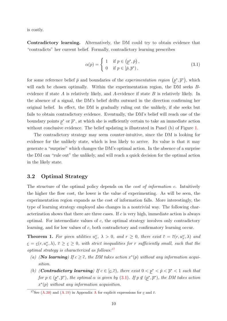
Contradictory learning. Alternatively, the DM could try to obtain evidence that

“contradicts” her current belief. Formally, contradictory learning prescribes

α(p) =

1 if p ∈

(p∗, p

),

0 if p ∈ [p, p∗) ,(3.1)

for some reference belief p and boundaries of the experimentation region(p∗, p∗

), which

will each be chosen optimally. Within the experimentation region, the DM seeks B-

evidence if state A is relatively likely, and A-evidence if state B is relatively likely. In

the absence of a signal, the DM’s belief drifts outward in the direction confirming her

original belief. In effect, the DM is gradually ruling out the unlikely, if she seeks but

fails to obtain contradictory evidence. Eventually, the DM’s belief will reach one of the

boundary points p∗ or p∗, at which she is sufficiently certain to take an immediate action

without conclusive evidence. The belief updating is illustrated in Panel (b) of Figure 1.

The contradictory strategy may seem counter-intuitive, since the DM is looking for

evidence for the unlikely state, which is less likely to arrive. Its value is that it may

generate a “surprise” which changes the DM’s optimal action. In the absence of a surprise

the DM can “rule out” the unlikely, and will reach a quick decision for the optimal action

in the likely state.

3.2 Optimal Strategy

The structure of the optimal policy depends on the cost of information c. Intuitively

the higher the flow cost, the lower is the value of experimenting. As will be seen, the

experimentation region expands as the cost of information falls. More interestingly, the

type of learning strategy employed also changes in a nontrivial way. The following char-

acterization shows that there are three cases. If c is very high, immediate action is always

optimal. For intermediate values of c, the optimal strategy involves only contradictory

learning, and for low values of c, both contradictory and confirmatory learning occur.

Theorem 1. For given utilities uωx , λ > 0, and r ≥ 0, there exist c = c(r, uωx , λ) and

c = c(r, uωx , λ), c ≥ c ≥ 0, with strict inequalities for r sufficiently small, such that the

optimal strategy is characterized as follows:17

(a) (No learning) If c ≥ c, the DM takes action x∗(p) without any information acqui-

sition.

(b) (Contradictory learning) If c ∈ [c, c), there exist 0 < p∗ < p < p∗ < 1 such that

for p ∈ (p∗, p∗), the optimal α is given by (3.1). If p 6∈ (p∗, p∗), the DM takes action

x∗(p) without any information acquisition.

17See (A.20) and (A.19) in Appendix A for explicit expressions for c and c.

10

(c) (Contradictory and Confirmatory learning) If c < c, then there exist 0 <

p∗ < p < p∗ < p < p∗ < 1 such that for p ∈ (p∗, p∗), the optimal α is given by

α(p) =

1, if p ∈(p∗, p

),

0, if p ∈(p, p∗

),

12

if p = p∗,

1, if p ∈ (p∗, p) ,

0, if p ∈ (p, p∗) .

(3.2)

If p 6∈ (p∗, p∗) the DM takes action x∗(p) without any information acquisition.

We sketch the main steps of the proof in Section 3.4 below. The formal proof can be

found in Appendix A.

The optimal policy in case (b) is depicted in Panel (b) of Figure 1. In case (c) the

pattern is more complex (see Panel (c) of Figure 1). Both confirmatory and contradictory

learning are optimal for some beliefs. Theorem 1 also states that the confirmatory re-

gion (p, p) is always sandwiched between two regions where the contradictory strategy is

employed. That is, near the boundaries of the experimentation region, the contradictory

strategy is always optimal.

The intuition for the optimal strategy is explained as follows. First, since learning is

costly, there are levels of confidence, given by p∗ and p∗, that the DM finds sufficient for

making decisions without any evidence. These beliefs constitute the boundaries of the

experimentation region; more extreme beliefs result in an immediate action.

Within the experimentation region (p∗, p∗), the DM’s choice depends on the trade-off

between the confirmatory and contradictory strategies. The confirmatory strategy has

the advantage that the DM will eventually discover evidence, and will thus never make

a mistake. At the same time, full discovery of evidence could lead to a long delay. This

is particularly the case when the DM is fairly certain in her belief. In that case, the

contradictory strategy becomes relatively more appealing. Suppose for instance the DM’s

belief p < p∗ is very close to p∗. In that case, the contradictory strategy either yields a

“surprise” (B-evidence), leading to a perfectly accurate decision b, or (more likely) allows

the DM to “rule out” the unlikely state B and reach the desired level of confidence p∗

for action a with very little delay. Of course, the DM could instead look for A-evidence

only briefly and take an action if no information arrives, but obtaining A-evidence has

no value since it does not change her action. The only sensible alternative is to “go all

the way” toward full discovery—i.e., the confirmatory strategy, but it takes a long time.

Hence, the contradictory strategy is optimal near the stopping boundaries. As the DM

becomes less certain, however, the trade-off tilts toward the confirmatory strategy, as the

contradictory strategy involves a longer delay to reach the stopping region.

11

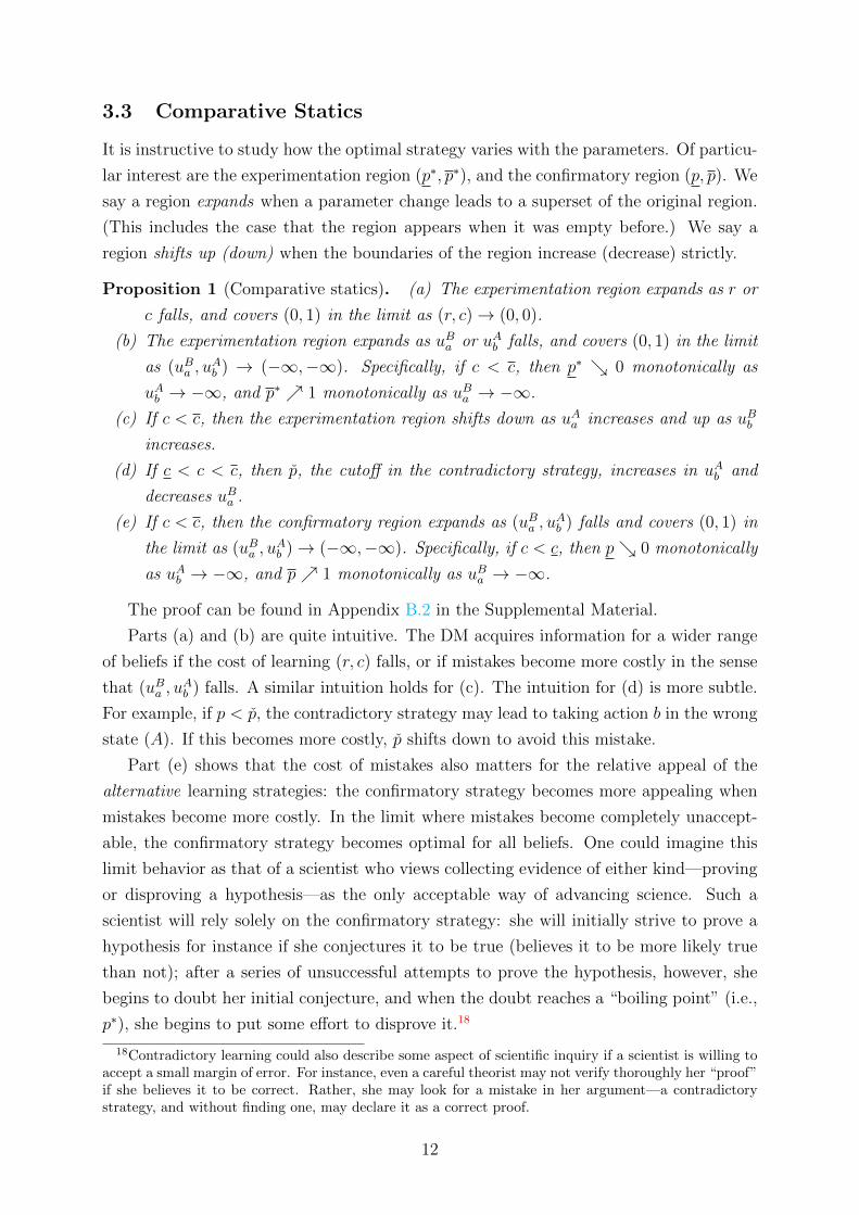
3.3 Comparative Statics

It is instructive to study how the optimal strategy varies with the parameters. Of particu-

lar interest are the experimentation region (p∗, p∗), and the confirmatory region (p, p). We

say a region expands when a parameter change leads to a superset of the original region.

(This includes the case that the region appears when it was empty before.) We say a

region shifts up (down) when the boundaries of the region increase (decrease) strictly.

Proposition 1 (Comparative statics). (a) The experimentation region expands as r or

c falls, and covers (0, 1) in the limit as (r, c)→ (0, 0).

(b) The experimentation region expands as uBa or uAb falls, and covers (0, 1) in the limit

as (uBa , uAb ) → (−∞,−∞). Specifically, if c < c, then p∗ 0 monotonically as

uAb → −∞, and p∗ 1 monotonically as uBa → −∞.

(c) If c < c, then the experimentation region shifts down as uAa increases and up as uBbincreases.

(d) If c < c < c, then p, the cutoff in the contradictory strategy, increases in uAb and

decreases uBa .

(e) If c < c, then the confirmatory region expands as (uBa , uAb ) falls and covers (0, 1) in

the limit as (uBa , uAb )→ (−∞,−∞). Specifically, if c < c, then p 0 monotonically

as uAb → −∞, and p 1 monotonically as uBa → −∞.

The proof can be found in Appendix B.2 in the Supplemental Material.

Parts (a) and (b) are quite intuitive. The DM acquires information for a wider range

of beliefs if the cost of learning (r, c) falls, or if mistakes become more costly in the sense

that (uBa , uAb ) falls. A similar intuition holds for (c). The intuition for (d) is more subtle.

For example, if p < p, the contradictory strategy may lead to taking action b in the wrong

state (A). If this becomes more costly, p shifts down to avoid this mistake.

Part (e) shows that the cost of mistakes also matters for the relative appeal of the

alternative learning strategies: the confirmatory strategy becomes more appealing when

mistakes become more costly. In the limit where mistakes become completely unaccept-

able, the confirmatory strategy becomes optimal for all beliefs. One could imagine this

limit behavior as that of a scientist who views collecting evidence of either kind—proving

or disproving a hypothesis—as the only acceptable way of advancing science. Such a

scientist will rely solely on the confirmatory strategy: she will initially strive to prove a

hypothesis for instance if she conjectures it to be true (believes it to be more likely true

than not); after a series of unsuccessful attempts to prove the hypothesis, however, she

begins to doubt her initial conjecture, and when the doubt reaches a “boiling point” (i.e.,

p∗), she begins to put some effort to disprove it.18

18Contradictory learning could also describe some aspect of scientific inquiry if a scientist is willing toaccept a small margin of error. For instance, even a careful theorist may not verify thoroughly her “proof”if she believes it to be correct. Rather, she may look for a mistake in her argument—a contradictorystrategy, and without finding one, may declare it as a correct proof.

12

The Role of Discounting. Intuitively, one would interpret r as a cost of learning and

would thus expect that c and r are substitutes in the sense that a higher discount rate

requires a lower flow cost for the same structure to emerge. Formally, ∂c/∂r < 0 and

∂c/∂r < 0. The following proposition shows that this is indeed the case if at least one

loss payoff (uAb or uBa ) is not too small.

Proposition 2. (a) Suppose c > 0. Then ∂c/∂r < 0 iff U(p) > 0, which is equivalent

to uAa uBb − uAb uBa > 0.

(b) Suppose c > 0. Then ∂c/∂r < 0 if both uAa >∣∣uAb ∣∣ and uBb >

∣∣uBa ∣∣; ∂c/∂r > 0 if

minuAb , u

Ba

is sufficiently small.

The proof can be found in Appendix B.3 in the Supplemental Material. If both loss

payoffs uAb and uBa are negative and sufficiently large in absolute value, we have ∂c/∂r > 0

and ∂c/∂r > 0. A higher discount rate calls for more experimentation in this case.

Intuitively, if losses are sufficiently large, the DM would prefer to delay their realization,

which favors longer experimentation. This explains Part (a) of Proposition 2. Moreover,

large losses in case of a mistake increase the need for accuracy, favoring the confirmatory

strategy. This explains Part (b) of Proposition 2.

3.4 Sketch of the Proof

We now sketch the main arguments leading to Theorem 1 in several steps. A less techni-

cally interested reader may want to skip this section. Our method is first to “guess” the

structure of the policy and then to verify its optimality. To this end, we first compute the

value of alternative learning strategies. Taking an action immediately simply yields U(p).

To compute the value of the other strategies, we first obtain two ODEs by substituting

α = 0 and α = 1 in the HJB equation (2.3). For given boundary conditions (p,W ), where

p ∈ (0, 1), the ODEs admit unique solutions V0(p; p,W ) and V1(p; p,W ), respectively.

To compute the value of the confirmatory strategy, recall that it prescribes, for some

p∗ ∈ (0, 1), α = 1/2 until evidence arrives, whereupon the DM takes an action according

to the evidence. Let U(p) denote the value of this “stationary” strategy.19 We can then

use V (p∗) = U(p∗) as a boundary condition for the value function and obtain

Vcf (p) :=

V0(p; p∗, U(p∗)), for p ≤ p∗,

V1(p; p∗, U(p∗)), for p ≥ p∗.

We postulate smooth pasting at p∗ and require Vcf (p) ≥ U(p) for all p in a neighborhood

of p∗. This uniquely pins down the reference belief as p∗ =(ruBb + c

)/(ruAa + ruBb + 2c

).

19We have U(p) = λ2r+λ

(puAa + (1− p)uBb

)− 2c

2r+λ . Intuitively, without mistakes, the DM achieves the

“first-best” payoff puAa + (1− p)uBb , but discounted and net off the expected discounted flow cost.

13

0.2 0.4 0.6 0.8 1.00.0

0.2

0.4

0.6

0.8

1.0

0.2 0.4 0.6 0.8 1.00.0

0.2

0.4

0.6

0.8

1.0

U(p)

Vct(p)

Vcf(p)

α(p)

U(p)

(a) c = .3 (only contradictory) (b) c = .15 (confirmatory and contradictory)

Figure 2: Value Function and Optimal Policy. The value function is the upper envelopeof Vct and Vcf (solid). (λ = 1, r = 0, uAa = 1, uBb = .9, uAb = uBa = −.9)

The value of contradictory learning is computed similarly. Intuitively, p∗ and p∗ are the

beliefs at which the DM is indifferent between an optimal immediate action and contradic-

tory learning for an instant followed by an immediate action in case of no discovery. This

yields the boundary conditions V (p∗) = Ub(p∗) and V (p∗) = Ua(p

∗). Next, we postulate

that the slope of the value is equal to U ′(p) at these values (smooth pasting). Combining

these two conditions pins down the critical beliefs p∗ and p∗. We can thus construct the

left branch and right branch of the value function for the contradictory strategy:

V ct(p) :=

Ub(p), if p ≤ p∗,

V1(p; p∗, Ub(p∗)), if p > p∗;

V ct(p) :=

Ua(p), if p ≥ p∗,

V0(p; p∗, Ua(p∗)), for p < p∗.

We combine these branches and construct the value of contradictory learning as Vct(p) :=

maxV ct(p), V ct(p)

.

Second, we consider a candidate solution VEnv(p) := maxVct(p), Vcf (p).20 In Propo-

sition 6, we show that this yields the strategies stated in Theorem 1. Two observations are

crucial. First, consider a hypothetical “full attention payoff”—the payoff the DM would

attain if she could set α = β = 1.21 We show that contradictory learning achieves this

upper bound at the stopping boundaries p∗ and p∗, while confirmatory learning achieves a

strictly lower value (Lemmas 3 and 4). This implies that contradictory learning is always

part of the optimal strategy since it dominates confirmatory learning at the stopping

boundaries p∗ and p∗. Second, we establish a Crossing Property (Lemma 5): a solution

V1(p;x,W ) can cross V0(p;x′,W ′) only from above if they exceed U(p). This means that

branches of the confirmatory and contradictory value function must intersect in the way

illustrated in Figure 2. In particular, this implies that the choice between confirmatory

and contradictory learning leads to one of the structures in Panels (b) and (c) of Figure

20This value is obtained if the DM chooses optimally between confirmatory and contradictory learningbased on the prior belief, and never switches.

21Choosing α = β = 1 is not feasible for the DM in our model with limited attention. The payoff fromα = β = 1 is only used as a benchmark.

14

1.22 Case (b) of Theorem 1 arises if Vct(p∗) ≥ U(p∗) and case (c) arises if Vct(p

∗) < U(p∗).

Finally, we show that the candidate VEnv(p) is the value function by verifying that it

satisfies the HJB equation (2.3). Since VEnv(p) is not everywhere differentiable, we show

that it is a viscosity solution of the HJB equation. By Theorem III.4.11 in Bardi and

Capuzzo-Dolcetta (1997), this implies that it is the value function of the DM’s problem.

4 Applications

The model of information acquisition with limited attention can be applied in various

situations. We discuss two applications: jury deliberation and media choice by voters.

For each we also discuss generalizations that go beyond the baseline model: In the case

of jury deliberation we consider the inclusion of a third action (a “hung jury”) and the

case of media choice, we consider news media with varying degrees of informativeness.

The formal treatment of the extensions can be found in Appendices D and E in the

Supplemental Material.

4.1 Jury Deliberation

In many states of the USA, when a prosecutor accuses an individual of a crime, a grand

jury is impaneled to decide whether to indict the accused. Should that occur, a trial

jury hears the case presented by the prosecutor and the defense attorney before returning

its verdict. Both types of juries deliberate based on the evidence or lack thereof over a

period of time. Our model can be used to consider their deliberation behavior and its

implications on the outcome.

Suppose that the DM is a member of a jury deciding whether to “indict/convict”

(action a) or “not indict/acquit” (action b) a defendant.23 The state is either “guilty”

(ω = A) or “innocent” (ω = B). Suppose the jury has already heard all the evidence

presented in the courtroom,24 and has formed a preliminary opinion summarized by the

prior belief p0. The jury proceeds with deliberation which involves revisiting the evidence,

testimonies, and arguments presented to them and scrutinizing some details jurors may

have missed (i.e., juries often ask for transcripts of testimonies they wish to scrutinize).

The attention decision α corresponds to the type of evidence/testimony that the jury may

scrutinize in depth.

22Note that as postulated in footnote 20, the DM never switches the mode of learning.23Here, we view the DM as a single juror, or a coalition of jurors acting like a single individual. The

conclusions would also apply for a single judge. In practice, the collective action aspect of jury deliberationbrings another layer to the problem, which is beyond the scope of this paper. See Persico (2004),Stephenson (2010), and Chan, Lizzeri, Suen, and Yariv (2016). Our application to jury deliberation is afirst step toward exploring information choice in the jury context.

24Only the prosecutor presents the case in grand jury proceedings, whereas in a trial, both prosecutorand defense attorney present the evidence.

15

0.2 0.4 0.6 0.8 1.00.0

0.2

0.4

0.6

0.8

1.0

0.2 0.4 0.6 0.8 1.00.0

0.2

0.4

0.6

0.8

1.0

0.2 0.4 0.6 0.8 1.00.0

0.2

0.4

0.6

0.8

1.0

U(p)

V (p)

α(p)

(a) Grand Jury (uAb = −1, uBa = 0) (b) Trial Jury (uAb = 0, uBa = −1) (c) Trial jury with hung jury (uc = .7)

Figure 3: Deliberation of grand and trial juries. (λ = 1, r = 0, c = .2, uAa = uBb = 1.)

One salient difference between the two juries is the costs of making alternative errors:

while a trial jury perceives a high cost of convicting an innocent (i.e., a low value of uBa ),

a grand jury must be more concerned about failing to indict a guilty defendant (i.e., a

low value of uAb ). The evidentiary standards as well as the decision rule employed by US

courts reflect this difference.25 Proposition 1 predicts how this difference causes grand

juries and trial juries to deliberate differently, and shows that the de facto evidentiary

standards—reflected by the boundaries p∗ and p∗—differ for the two juries.

For ease of exposition we use examples to illustrate our findings which hold generally.

Panels (a) and (b) of Figure 3 depict examples where the parameters are chosen so that

Part (b) of Theorem 1 obtains.

For the grand jury in panel (a), probable cause corresponds to p > p∗ = .8. If the prior

falls in this range, the jury returns an indictment right away. Conversely, the accused

is acquitted immediately only if p0 < p∗ = .1. This shows that the stronger concern

about acquitting a guilty person leads the grand jury to require a higher standard for

this decision. If the grand jury does not return a decision immediately, for most beliefs

(p ∈ (.17, .8) in the example), the jury will look for exculpatory evidence.26 If no such

evidence is found, the jury becomes more convinced that there is “probable cause,” and

ultimately returns an indictment.

The trial jury deliberates differently. The evidentiary standard for conviction is higher

(p∗ = .9 in the example), whereas the standard for acquittal is lower (p∗ = .2), reflect-

ing the greater concern about convicting an innocent person. Moreover, if no immediate

verdict is returned, for most beliefs (p ∈ (.2, .83) in the example), the jury scrutinizes

incriminating evidence. Not finding such evidence pushes the jury’s belief toward “rea-

sonable doubt” and an acquittal.

In many cases, unanimity is required for a jury decision. If no consensus is reached, a

hung jury arises. In the US this leads to a mistrial with the possibility to retry the case.

Although a consequence of unanimity rule adopted by Common Law courts for criminal

25In a criminal case, conviction in a criminal court requires proving guilt “beyond the reasonabledoubt” whereas the standard for grand jury indictment is “probable cause.” The decision rule for trialjury is unanimity, whereas a grand jury indictment requires concurrence by 12 members out of 16-23total members.

26If uAa = uBb and uBa > uAb , then p∗ < 1− p∗ by part (b), and p < 1/2 by part (d) of Proposition 1.

16

cases, in principle a mistrial need not be the only solution to a jury deadlock,27 and its

effect on jury deliberation is an important question. To analyze the effect, we introduce

hung jury in “reduced form” as a third action c, which we assume to have a safe payoff

of uAc = uBc = uc.28 Panel (c) of Figure 3 depicts this case for a trial jury. The effects of

introducing the option of a hung jury can be summarized as follows.

First, the possibility of a hung jury does not change the evidentiary standard for either

verdict: they remain p∗ = .2 for acquittal and p∗ = .9 for conviction. The reason is that

these standards are set by indifference between contradictory learning and immediate

action, and the values of these strategies are not affected by the hung jury option.

Second, the hung jury option affects the deliberation strategy in favor of seeking in-

criminating evidence (B-evidence). The value of seeking incriminating evidence increases

since the jury faces a more appealing option, namely to “settle” for mistrial instead

of deliberating until they reach the reasonable doubt. This means that for some pre-

deliberation beliefs (p0 ∈ [.83, .85]), the jury switches attention from exculpatory evi-

dence to incriminating evidence. The flip side of this behavior is that for a large range of

pre-deliberation beliefs (p0 ∈ [.35, .67]) a mistrial is declared.

Third, the change in deliberation behavior also affects verdicts. For p0 ∈ [.67, .85]), the

probability of guilty verdict falls.29 Remarkably, the probability of “not-guilty” verdict

also falls. In fact, with the mistrial option, the jury never returns a “not-guilty“ verdict

for any pre-deliberation belief p0 ∈ [.35, .85] above the lower bound of the mistrial region,

whereas, without that option, the jury would have returned “not guilty” verdict with

positive probability after a long deliberation (when it reaches p∗).

These findings suggest that the possibility of hung jury has complex and nontrivial

effects on jury deliberation and verdicts and also point to the richness of the prediction

that can be brought out by use of a dynamic model such as the current one.30

27For instance, in England and New Zealand, the unanimity requirement is relaxed in the event of a jurydeadlock, allowing a judge to require supermajority instead. Hung jury is not possible in a Scottish courtwhere a simple majority is required for a verdict. See https://en.wikipedia.org/wiki/Hung_jury.

28An interpretation is that this is a continuation value jurors assign to a mistrial. We formally analyzethe model with a third action in Appendix D in the Supplemental Material.

29Fix any belief p0 ∈ [0.83, 0.85] in the switching region. Without hung jury, the probability of a guiltyverdict exceeds p0 since the jury never finds the guilty innocent whereas it may find the innocent guilty(in case the jury reaches p∗ without finding exculpatory evidence). With hung jury, the probability ofguilty verdict falls strictly below p0 by an analogous argument. For p0 ∈ [0.67, 0.83], mistrial is declaredin any event in which, without hung jury, the jury would have found incriminating evidence after p fellbelow 0.67. Hence, the probability of a guilty verdict is reduced commensurately.

30The analysis so far focused on the situation in which, without hung jury, jury deliberation involvesonly contradictory learning. The case with both confirmatory and contradictory learning is analogous:introduction of mistrial increases the value of confirmatory learning, which reduces the probability of theguilty verdict for high p (around p) and that of the not guilty verdict for a low p (around p), at theexpense of increased probability of mistrial.

17

state B

state A

no factual information

no factual information

B-evidence

A-evidence

facts (B-favoring)rhetoric (A-favoring)

rhetoric (A-favoring)

state B

state A

no factual information

no factual information

B-evidence

A-evidence

facts (A-favoring)

rhetoric (B-favoring)

rhetoric (B-favoring)

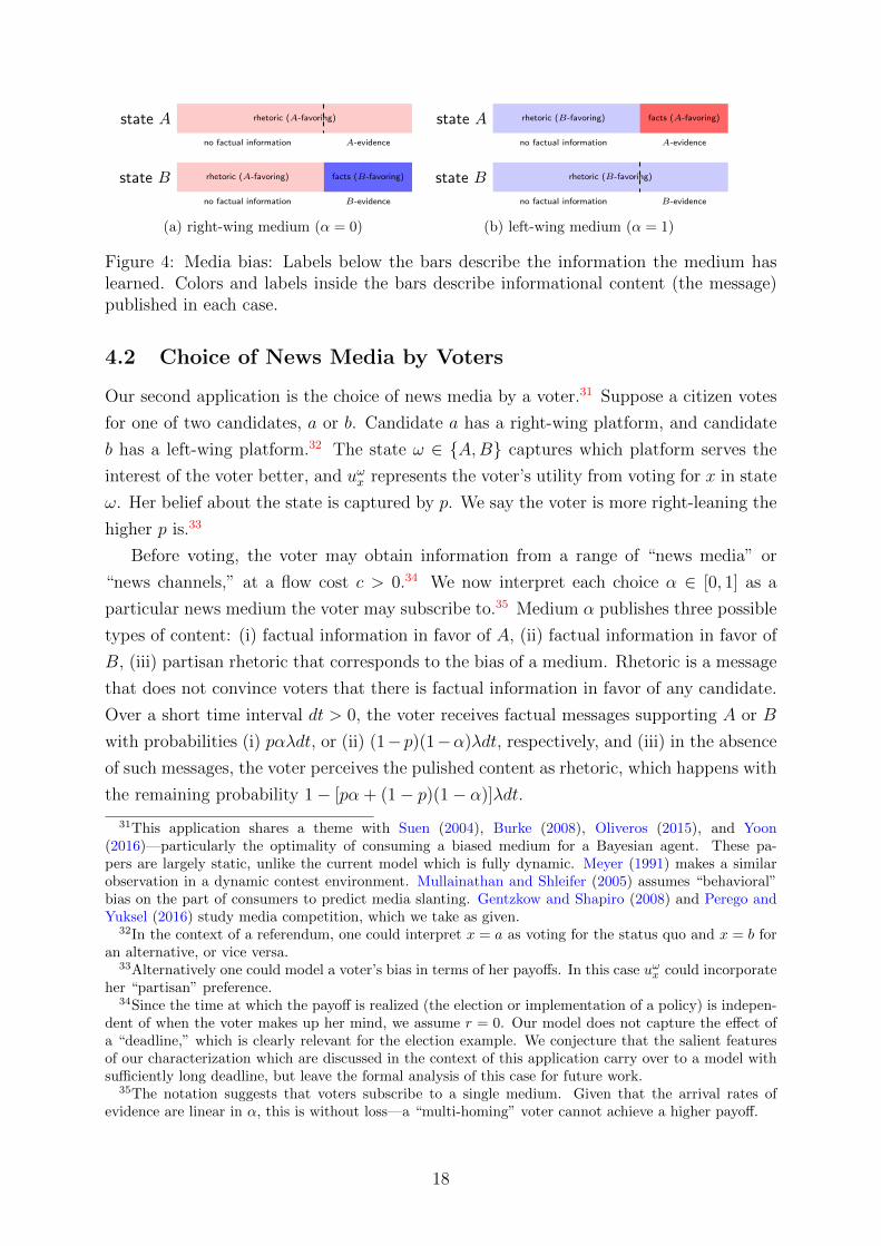
(a) right-wing medium (α = 0) (b) left-wing medium (α = 1)

Figure 4: Media bias: Labels below the bars describe the information the medium haslearned. Colors and labels inside the bars describe informational content (the message)published in each case.

4.2 Choice of News Media by Voters

Our second application is the choice of news media by a voter.31 Suppose a citizen votes

for one of two candidates, a or b. Candidate a has a right-wing platform, and candidate

b has a left-wing platform.32 The state ω ∈ A,B captures which platform serves the

interest of the voter better, and uωx represents the voter’s utility from voting for x in state

ω. Her belief about the state is captured by p. We say the voter is more right-leaning the

higher p is.33

Before voting, the voter may obtain information from a range of “news media” or

“news channels,” at a flow cost c > 0.34 We now interpret each choice α ∈ [0, 1] as a

particular news medium the voter may subscribe to.35 Medium α publishes three possible

types of content: (i) factual information in favor of A, (ii) factual information in favor of

B, (iii) partisan rhetoric that corresponds to the bias of a medium. Rhetoric is a message

that does not convince voters that there is factual information in favor of any candidate.

Over a short time interval dt > 0, the voter receives factual messages supporting A or B

with probabilities (i) pαλdt, or (ii) (1−p)(1−α)λdt, respectively, and (iii) in the absence

of such messages, the voter perceives the pulished content as rhetoric, which happens with

the remaining probability 1− [pα + (1− p)(1− α)]λdt.

31This application shares a theme with Suen (2004), Burke (2008), Oliveros (2015), and Yoon(2016)—particularly the optimality of consuming a biased medium for a Bayesian agent. These pa-pers are largely static, unlike the current model which is fully dynamic. Meyer (1991) makes a similarobservation in a dynamic contest environment. Mullainathan and Shleifer (2005) assumes “behavioral”bias on the part of consumers to predict media slanting. Gentzkow and Shapiro (2008) and Perego andYuksel (2016) study media competition, which we take as given.

32In the context of a referendum, one could interpret x = a as voting for the status quo and x = b foran alternative, or vice versa.

33Alternatively one could model a voter’s bias in terms of her payoffs. In this case uωx could incorporateher “partisan” preference.

34Since the time at which the payoff is realized (the election or implementation of a policy) is indepen-dent of when the voter makes up her mind, we assume r = 0. Our model does not capture the effect ofa “deadline,” which is clearly relevant for the election example. We conjecture that the salient featuresof our characterization which are discussed in the context of this application carry over to a model withsufficiently long deadline, but leave the formal analysis of this case for future work.

35The notation suggests that voters subscribe to a single medium. Given that the arrival rates ofevidence are linear in α, this is without loss—a “multi-homing” voter cannot achieve a higher payoff.

18

The informational content of partisan rhetoric—and thus the partisan bias—depends

on the medium α. To illustrate this, consider the most extreme media. (Media bias

for the general case 0 ≤ α ≤ 1 is more precisely micro-founded in Appendix C of the

Supplemental Material.) As depicted in Panel (a) of Figure 4, medium α = 0 sends B

messages in state B only when it learns facts supporting B, which happens with some

probability. Otherwise it sends partisan rhetoric favoring the right-wing candidate a both

in state B and in state A.36 We therefore call medium α = 0 right-wing. Intuitively,

a right-wing medium will advocate the left-wing candidate b only if it possesses hard

facts supporting state B. On the other hand, it is willing to advocate the right-wing

candidate even in the absence of factual information. Therefore, even if it possesses

factual information in favor of a, voters will not distinguish this from partisan rhetoric.

As depicted in Panel (b), medium α = 1 has the opposite bias. It always publishes

(left-wing) rhetoric in state B. In state A it also publishes left-wing rhetoric, except when

it learns factual evidence in favor of candidate a. Corresponding to the bias of the rhetoric

we call such a medium left-wing. More generally, a medium α ∈ (0, 1/2) is moderately

right-wing, a medium α ∈ (1/2, 1) is moderately left-wing, and the medium α = 1/2 is

called unbiased.

We treat the behavior of media as exogenous to the model and focus on optimal

subscription choices by voters for a given set of media. With this interpretation of the

model, Theorem 1 has the following implications for the choice of news media.

Corollary 1. Voters with extreme beliefs p /∈(p∗, p∗

)always vote for their favorite candi-

dates without consulting media. Those subscribing to media exhibit the following behavior.

(a) (Moderately informative media) Suppose c ≤ c < c:

• All voters to the right of p subscribe to right-wing media and all voters to the

left of p subscribe to left-wing media.

• Over time absent breakthrough news, all voters become progressively more ex-

treme and polarized.

(b) (Highly informative media) Suppose c < c:

• (i) Right-leaning voters (p ∈ (p, p∗)) and moderate left-leaning voters (p ∈(p, p∗)) subscribe to right-wing media. (ii) Left-leaning voters (p ∈ (p∗, p)) and

moderate right-leaning voters (p ∈ (p∗, p)) subscribe to left-wing media. (iii)

Undecided voters (p = p∗) subscribe to unbiased media.

• Over time absent breakthrough news, moderate voters (p ∈(p, p)) become in-

creasingly undecided and more extreme voters become increasingly more ex-

treme and polarized.

Panel (a) of Figure 5 shows the choice of media α by voters with different beliefs.

36Note that the partisan bias of the rhetoric is consistent with Bayesian updating. Since rhetoric ismore frequent in state A, it must be in favor of the right-wing candidate.

19

0.0 0.2 0.4 0.6 0.8 1.00.0

0.2

0.4

0.6

0.8

1.0

0.2 0.4 0.6 0.8 1.00.0

0.2

0.4

0.6

0.8

1.0

|—bp∗

left︷ ︸︸ ︷←−←−α=1

p

right︷ ︸︸ ︷−→−→α=0

unb.︷ ︸︸ ︷p∗

α=12

left︷ ︸︸ ︷←−←−α=1

p

right︷ ︸︸ ︷−→−→α=0

p∗—a| |—

bp∗

left︷ ︸︸ ︷←−←−α> 1

2

p

right︷ ︸︸ ︷−→−→α< 1

2

unb.︷ ︸︸ ︷p∗

α=12

left︷ ︸︸ ︷←−←−α> 1

2

p

right︷ ︸︸ ︷−→−→α< 1

2

p∗—a|

(a) constant informativeness (λ = 1, c = .2) (b) variable informativeness (c = .35)

Figure 5: Optimal media choice. (r = 0, uAa = uBb = 1, uBa = uAb = −1)

Figure 6 shows how the distribution of beliefs evolves over time (measured at three dif-

ferent times), where colors represent the media choice by voters who are still subscribing

to media. The initial distribution is p0 ∼ U [0, 1] in this example.

Among those subscribing to news media, voters on the far right choose right-wing

media. Such a medium is valuable to them since it mostly publishes a content reinforcing

their belief, and publishes left-favoring information only if it is accurate enough (in fact,

fully conclusive in the baseline model) to actually convince them to change their votes.

Over time, in the absence of convincing contradictory news, the right-wing medium feeds

such voters with what they believe, leading them to become more extreme in their beliefs.

Hence, applied to dynamic media choice with fully Bayesian voters, our model generates

self reinforcing beliefs—sometimes called an “echo-chamber” effect—that persists until

strong contradictory evidence arrives.

The moderately right voter’s media choice is quite different. Their moderate beliefs

cause them to seek accurate evidence (of either kind) for voting. Initially they look

for right-favoring evidence which they expect more likely to arise given their beliefs.

Interestingly, they expect to find such evidence in left-wing media, since these media

scrutinize the right-favoring information more and apply a very high standard for reporting

t=0.

0.0 0.2 0.4 0.6 0.8 1.00.0

0.5

1.0

1.5

2.0 Density

t=0.210168

0.0 0.2 0.4 0.6 0.8 1.0

t=0.766722

0.0 0.2 0.4 0.6 0.8 1.00.

0.0625

0.125

0.1875

0.25Mass

Figure 6: Evolution of media choice and beliefs when the true state is B. Shaded areasrepresent the density of beliefs (left axis). Bold bars represent mass points of beliefs (rightaxis).

20

such information. The moderate’s media choice thus differs from the extreme voter’s

choice. The prediction of an “anti-echo chamber” effect is novel and has no analogue in

previous literature. Over time, absent breakthrough news, their anti-echo chamber choice

leads voters to be undecided. Ultimately, they switch to the unbiased medium.

In sum, our dynamic model of media choice predicts two different dynamics of belief

evolution resulting from optimal media choice: the beliefs for those who are sufficiently

extreme become more polarized, and the beliefs of those who are sufficiently moderate

converge toward the middle and result in the subscription of unbiased media.

Trade-off between Skewness and Informativeness of Media. One prediction of

the baseline model is that voters only choose from three media, right-wing, left-wing,

and unbiased. This is a consequence of the assumption that all media have access to

information with identical arrival rates, and differ only in the rhetoric they publish. For-

mally, each news medium is characterized by a pair of arrival rates (λA, λB) for A- and

B-evidence, respectively. The sum of arrival rates λA +λB can be viewed as a measure of

the informativeness of a medium. In the baseline model, if we normalize λ = 1, we have

λA = α and λB = β = 1− α, so that λA + λB = 1 for all media. The analysis of this case

suggests that there is no demand for moderate media and the market will be dominated

by extremely-biased outlets, as long as all media are identical in their informativeness.

We relax this assumption and introduce a trade-off between bias and informativeness

by assuming less biased media to be more informative. This generates predictions about

which voters have a stronger preference for informativeness versus bias.

Formally we assume that λB = Γ(λA), where Γ(λA) is a decreasing concave function,

and set α = λA/(λA + Γ(λA)

). The interpretation is that news outlets that are more

balanced have access to more factual information, for example because they employ jour-

nalists focused more on hard evidence.37 In Appendix E in the Supplemental Material,

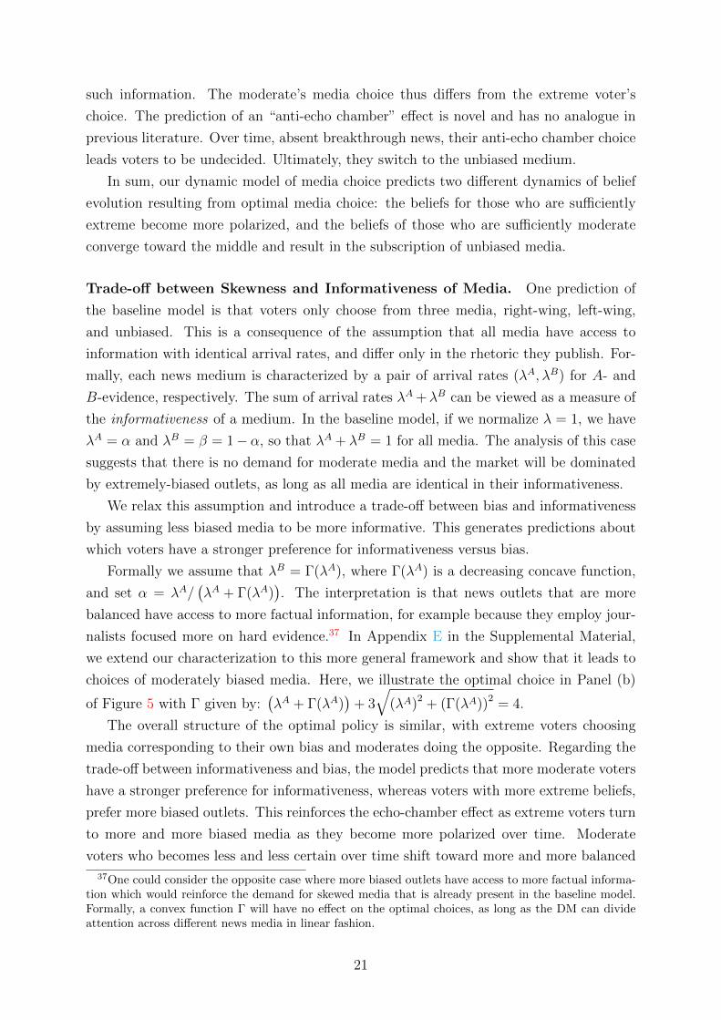
we extend our characterization to this more general framework and show that it leads to

choices of moderately biased media. Here, we illustrate the optimal choice in Panel (b)

of Figure 5 with Γ given by:(λA + Γ(λA)

)+ 3√

(λA)2 + (Γ(λA))2 = 4.

The overall structure of the optimal policy is similar, with extreme voters choosing

media corresponding to their own bias and moderates doing the opposite. Regarding the

trade-off between informativeness and bias, the model predicts that more moderate voters

have a stronger preference for informativeness, whereas voters with more extreme beliefs,

prefer more biased outlets. This reinforces the echo-chamber effect as extreme voters turn

to more and more biased media as they become more polarized over time. Moderate

voters who becomes less and less certain over time shift toward more and more balanced

37One could consider the opposite case where more biased outlets have access to more factual informa-tion which would reinforce the demand for skewed media that is already present in the baseline model.Formally, a convex function Γ will have no effect on the optimal choices, as long as the DM can divideattention across different news media in linear fashion.

21

outlets. Overall, absent breakthrough news, demand for outlets with moderate biases falls

over time, as extreme voters become more extreme and switch to more extreme media;

and moderate voters become more moderate and eventually subscribe to balanced media.

5 Generalized Model with Non-Conclusive Evidence

In the baseline model, we have assumed that the DM can access fully revealing signals.

We now generalize the model to allow for the signals to be noisy. A-signals now arrive at

rate λ in state A, and at rate λ in state B, where we assume λ > λ ≥ 0. Importantly,

the DM does not observe the state generating these signals. Similarly, B-signals arrive at

rate λ in state B, and at rate λ in state A.38 If λ = 0, the signals are fully revealing, and

we obtain the baseline model. We impose the following assumption

Assumption 1. Either r = 0, or uAa λ+ uAb λ > 0 and uBb λ+ uBa λ > 0.

This assumption means that losses associated with the wrong action are not too large.

Without this assumption, delayed action may be beneficial because this leads to dis-

counting of losses. The DM would prefer to learn as slowly as possible. Assumption 1

guarantees that for all c ≥ 0, the DM has a preference to speed up learning.39

With noisy signals, the DM may find it optimal to wait for more than one signal before

taking an action. Our characterization from the baseline model generalizes naturally, if

the DM finds it optimal not to wait for multiple signals. In this case, we say the model

satisfies the single experimentation property (SEP). We provide a necessary and sufficient

condition for SEP in terms of a critical cost level and characterize the optimal strategy

under SEP. In Section 6, we illustrate what the optimal strategy looks like when SEP

does not hold.

5.1 Optimal Strategy under SEP

As in the baseline model, the DM’s attention strategy determines which signals are actu-

ally observed. If she allocates a fraction α ∈ [0, 1] of her attention to seeking A-signals and

β = 1− α to seeking B-signals, she receives an A-signal with arrival rate αλA(p), where

λA(p) := pλ+(1−p)λ. An A-signal leads to a posterior qA(p) := λp/(λp+ λ(1− p)

)> p.

Similarly B-signals arrive at rate (1−α)λB(p) where λB(p) := pλ+ (1− p)λ, and lead to

posterior qB(p) := λp/(λp+ λ(1− p)

)< p. If the DM does not receive any signal, her

belief evolves according to pt = − (2αt − 1) δpt(1− pt), where δ := λ− λ denotes the dif-

ference in arrival rates between signal and noise. We now state the optimal strategy, with

38Allowing the DM to choose any signal with state contingent arrival rates (λA, λB) ∈ [λ, λ]2 does notchange the analysis; the DM will optimally choose only between (λA, λB) = (λ, λ) and (λA, λB) = (λ, λ).

39We could instead impose weaker conditions that depend on c. In the proofs we use U(p) > U(p) forall p, c+ rUb(p

∗) ≥ 0 and c+ rUa(p∗) ≥ 0. These are implied by Assumption 1.

22

the detailed analysis and explicit definitions relegated to Appendix A. As before, the opti-

mal policy is a combination of immediate action, contradictory learning and confirmatory

learning.

Theorem 2. For any (r, uωx , λ, λ), there exists a critical cost-level cSEP = cSEP(r, uωx , λ, λ) ≥0 such that SEP holds if and only if c ≥ cSEP.40 Given c ≥ cSEP, there exists c =

c(r, uωx , λ, λ) > 0 such that the optimal strategy is characterized as follows:

(a) Suppose c ≥ c. Then the DM takes an optimal action x∗(p) without information

acquisition.

(b) Suppose c ∈[cSEP, c

). For p ∈ (p∗, p∗), the optimal strategy takes either the con-

tradictory form (3.1) or the mixed contradictory and confirmatory form (3.2). For

p 6∈ (p∗, p∗), it is optimal to take an immediate action. In particular, (3.1) is optimal

for c in a neighborhood of c, and (3.2) is optimal for c in a neighborhood of cSEP if

r and λ are both sufficiently low.

5.2 Implications for Stochastic Choice and Response Time

The general model exhibits rich implications for the choice process. We explore them and

compare them with some well-known benchmarks. In classic models such as Luce’s logit

model, stochastic choice can be interpreted as arising from unobserved random utility.

In contrast, in models of information acquisition such as Wald, RI, and DDM, as well

as our model, choice is stochastic because the DM learns the payoff-relevant state with

noise, so that the choice probabilities depend on the DM’s prior. This is not the case in

random-utility models. There is a particular structure to this dependence and we first

explore the predictions for the accuracy and delay of decisions across DMs with different

prior beliefs. Second, we explore the predicted time pattern of choice in a single DM with

a fixed prior.

Accuracy of decisions. A measure of the accuracy of the decision is the average

posterior belief that the DM holds when taking a particular action. This measure captures

the (subjective) probability that an action is optimal conditional on being chosen. In the

RI model, the accuracy does not vary with the DM’s initial belief for the range of priors

where the DM acquires information (Matejka and McKay, 2015). This property is also

shared by the DDM in which the DM makes a decision if and only if her belief drifts to

one of the stopping boundaries that are constant over time.41 The accuracy, or the belief,

at the boundary therefore determines the accuracy of the decision.

40We have cSEP = 0 if r > 0 and λ is sufficiently close to zero.41This holds in our framework with binary states and actions (Peskir and Shiryaev, 2006). Below we

will discuss the DDM with a continuum of states considered by Fudenberg, Strack, and Strzalecki (2017)which generates prior-dependence.

23

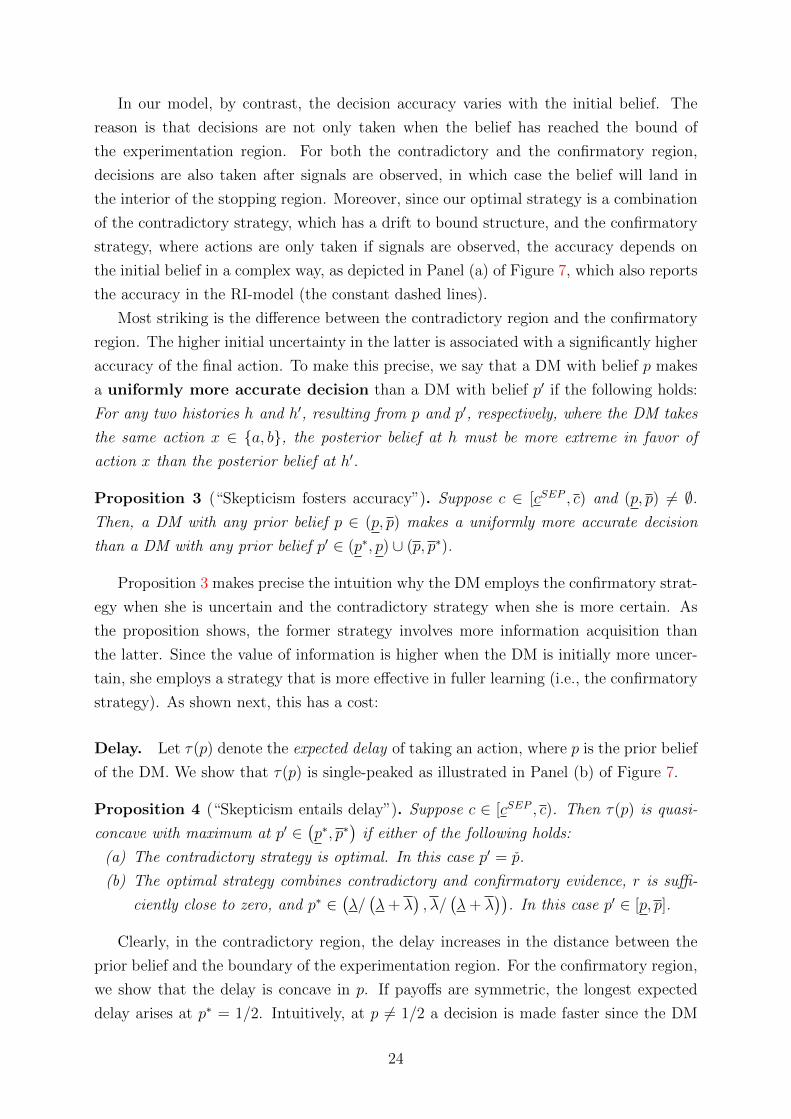
In our model, by contrast, the decision accuracy varies with the initial belief. The

reason is that decisions are not only taken when the belief has reached the bound of

the experimentation region. For both the contradictory and the confirmatory region,

decisions are also taken after signals are observed, in which case the belief will land in

the interior of the stopping region. Moreover, since our optimal strategy is a combination

of the contradictory strategy, which has a drift to bound structure, and the confirmatory

strategy, where actions are only taken if signals are observed, the accuracy depends on

the initial belief in a complex way, as depicted in Panel (a) of Figure 7, which also reports

the accuracy in the RI-model (the constant dashed lines).

Most striking is the difference between the contradictory region and the confirmatory

region. The higher initial uncertainty in the latter is associated with a significantly higher

accuracy of the final action. To make this precise, we say that a DM with belief p makes

a uniformly more accurate decision than a DM with belief p′ if the following holds:

For any two histories h and h′, resulting from p and p′, respectively, where the DM takes

the same action x ∈ a, b, the posterior belief at h must be more extreme in favor of

action x than the posterior belief at h′.

Proposition 3 (“Skepticism fosters accuracy”). Suppose c ∈ [cSEP , c) and (p, p) 6= ∅.Then, a DM with any prior belief p ∈ (p, p) makes a uniformly more accurate decision

than a DM with any prior belief p′ ∈ (p∗, p) ∪ (p, p∗).

Proposition 3 makes precise the intuition why the DM employs the confirmatory strat-

egy when she is uncertain and the contradictory strategy when she is more certain. As

the proposition shows, the former strategy involves more information acquisition than

the latter. Since the value of information is higher when the DM is initially more uncer-

tain, she employs a strategy that is more effective in fuller learning (i.e., the confirmatory

strategy). As shown next, this has a cost:

Delay. Let τ(p) denote the expected delay of taking an action, where p is the prior belief

of the DM. We show that τ(p) is single-peaked as illustrated in Panel (b) of Figure 7.

Proposition 4 (“Skepticism entails delay”). Suppose c ∈ [cSEP , c). Then τ(p) is quasi-

concave with maximum at p′ ∈(p∗, p∗

)if either of the following holds:

(a) The contradictory strategy is optimal. In this case p′ = p.

(b) The optimal strategy combines contradictory and confirmatory evidence, r is suffi-

ciently close to zero, and p∗ ∈(λ/(λ+ λ

), λ/

(λ+ λ

)). In this case p′ ∈ [p, p].

Clearly, in the contradictory region, the delay increases in the distance between the

prior belief and the boundary of the experimentation region. For the confirmatory region,

we show that the delay is concave in p. If payoffs are symmetric, the longest expected

delay arises at p∗ = 1/2. Intuitively, at p 6= 1/2 a decision is made faster since the DM

24

0.85

0.90

0.95

1.00

0.0 0.2 0.4 0.6 0.8 1.0

0.00

0.05

0.10

0.15

q˜a(p0)

q˜b(p0)

qa(p0)

qb(p0)

0.1 0.2 0.3 0.4 0.5 0.6 0.7 0.8 0.90.0

0.5

1.0

1.5

τ(p0)

(a) Accuracy (dotted: RI, solid: our model) (b) Expected Delay

Figure 7: Parameters: λ = 1, λ = .025, r = 0, c = 0.115, uAa = uBb = 1, uAb = uBa = 0.The weight of the cost function in the RI-model is µ = 1.025, which leads to identicalexperimentation regions in both models. Grid lines at: p∗, p, p∗, p, p∗ (left to right).

focuses her attention on the signal that is more likely to arrive.42 Finally, we show using

a revealed preference argument that at p and p, the delay in the contradictory strategy

must be shorter to compensate for the less accurate decision.

Similar results hold in the RI model and DDM. The difference is that in our model,

the two modes of learning lead to discontinuities in the average delay when the posterior

moves from the confirmatory to the contradictory region.43

Speed-Accuracy Complementarity. So far, we have analyzed properties of the stochas-

tic choice as a function of the prior belief. Next, we obtain a prediction on how, for a

given prior, the accuracy varies as a function of decision time.

Proposition 5. Suppose c ∈ [cSEP , c). For a DM with belief in p0 ∈ [p∗, p] ∪ [p∗, p],

conditional on taking a, a later decision results in lower accuracy. For a DM with p0 ∈[p, p∗] ∪ [p, p∗], conditional on choosing b, a later decision results in lower accuracy.

We obtain speed-accuracy complementarity, meaning later decisions tend to be less

accurate. The reason is that (regardless of the prior), the DM becomes less and less

convinced of the state she is seeking evidence for. Hence, if she discovers, say A-evidence,

after a long period of waiting, she updates to a lower posterior than if she discovers

A-evidence quickly (formally, qA(pt) < qA(p0)).

Whether a long delay produces a more or less accurate decision has been of consider-

able interest in cognitive psychology. In a typical experiment in this area, subjects make

42In the asymmetric case, p∗ differs from 1/2 so that the DM sometimes focuses attention on the lesslikely signals. τ is still concave in this case but the peak may differ from both p∗ and 1/2.

43In the static RI model, we can interpret the (average) cost incurred as delay and the result follows fromconcavity of mutual information. In the DDM, the result follows straightforwardly from the convexity ofthe value function (see Peskir and Shiryaev, 2006, Theorem 21.1).

25

choices over time—often of perceptual judgment type (see Ratcliff and McKoon, 2008,

for a survey). What emerges as a pattern is that decisions with a longer response time

tend to be less accurate. This phenomenon, known as speed-accuracy complementarity, is

difficult to explain via the DDM often used to fit the data, unless the stopping boundaries

collapse over time.44 Fudenberg, Strack, and Strzalecki (2017) justify collapsing bound-

aries by introducing rich uncertainty in terms of payoff differences between two actions,

and produce a less accurate decision over time.45 We obtain a similar prediction in a

Poisson model but the mechanism behind our result is different.46

6 Repeated Experimentation

So far we have focused on the situation in which the SEP holds, which requires the cost of

information acquisition to be sufficiently high (Theorem 2). We now discuss cases where

the SEP fails. In the examples we solve, the optimal solution retains the same structure as

in Theorems 1 and 2.47 In particular, the optimal policy combines immediate action, con-

firmatory and contradictory evidence. At the boundaries of the experimentation region,

it is still optimal to seek contradictory signals, and the confirmatory region appears if the

cost of information acquisition is sufficiently low. Unlike when SEP holds, however, the

DM may optimally switch between different modes of learning, as discovery of evidence

while following one strategy may lead to a posterior for which a different learning strategy

is prescribed.

Figure 8 depicts an optimal policy that exhibits one such pattern.48 The colored bars

indicate originating beliefs on top, and the corresponding regions where the posterior

lands after receiving a signal on the bottom. For instance, discovery made in top I will

44The DDM assumes that a subject’s perception follows a diffusion process with drift reflecting theunderlying stimulus. In DDMs with constant boundaries, the threshold beliefs for decisions do not changeover time, so a decision is made with the same accuracy over time, and speed-accuracy independencefollows. If the boundaries collapse over time, then a later decision is made with less extreme or moreuncertain beliefs, so speed-accuracy complementarity can be explained. See Drugowitsch, Moreno-Bote,Churchland, Shadlen, and Pouget (2012) and Hawkins, Forstmann, Wagenmakers, Ratcliff, and Brown(2015) for discussions of the DDM with collapsing boundaries and the related evidence.

45Given the uncertainty about payoff differences, a long passage of time without observing strongevidence in favor of either action indicates that payoff differences are likely to be small. This reduces theincentive to acquire further information, causing the DM to stop with lower accuracy.

46The extent to which Poisson signals accurately describe decision making in these experiments, orthe underlying neurophysiology, is not clear. Whether brain processes stimuli through a gradual processdescribed by DDM or a discrete process described by a Poisson model is subject of active researchin neuroscience (see Latimer, Yates, Meister, Huk, and Pillow (2015) for instance). Within a Poissonmodel, our reliance on SEP further limits the applicability of our model in explaining these experiments.Nevertheless, our finding points to the potential usefulness of a Poisson-based approach; we leave forfuture research extension of the current model toward this direction.

47Providing a general characterization is difficult since the number of possible strategies increases. Ouranalysis of examples studied in Appendix F in the Supplemental Material reveals both the difficultiesand the potential ways to overcome them.

48A plot of the value function and posterior as well as other cases can be found in Appendix F ofSupplemental Material.

26

Figure 8: Repeated Experimentation. λ = 1, λ = .2, r = 0, c = .1, uAa = uBb = 1, uAb =uBa = 0.

lead to a posterior in bottom I. In this example, discovery made in a contradictory region

(I-II and V-VI on the top) leads to a posterior in another part of the contradictory region

or in the confirmatory region, that is, it will never lead to an immediate action.49

The bottom graph of Figure 8 illustrates a possible evolution of the belief under the

optimal strategy. Suppose the DM has a prior belief p0 in top II region. She then looks

for A-evidence, as prescribed by contradictory learning. Her belief drifts down until she

discovers A-evidence. Suppose she does so at p1, still within region II. Her belief then

jumps up to p2 (in bottom II, or top V, region). Now she looks for B-evidence, as

prescribed by contradictory learning for that belief. Her belief drifts up until she finds

B-evidence. Suppose she does so at p3 in top VI region. Her belief then jumps down

to p4 in bottom VI, or top III, region, a confirmatory region where she again looks for

B-evidence. Suppose she discovers B-evidence at p5. This time her belief jumps down

to p6, in bottom region III, which is outside the experimentation region. She now picks

action b, completing the journey.

7 Conclusion

We have studied a model in which a decision maker may allocate her limited attention to

collecting different types of evidence that support alternative actions. Assuming Poisson

arrival of evidence, we have shown that the optimal policy combines immediate action,

contradictory learning, and confirmatory learning for different prior beliefs. We have

then used this characterization to yield rich predictions about information acquisition

and choices several in real-world settings.

We envision several avenues of extending the current work. First, our model is rela-

tively tractable (e.g., the value function and optimal policy are available in closed form).

49As in the case where SEP holds, a discovery made in the confirmatory region (top regions III-IV)leads to a posterior in the stopping region and an immediate action.

27

Therefore, we hope that this framework will be useful to integrate dynamic choice of infor-

mation in applied theory models. This includes our applications of jury and media choice,

which could be extended beyond our analysis in the present paper. Dynamic information

choice might be also embedded into a principal-agent setup in which a principal tries to

induce an agent to acquire information or a strategic setup such as R&D competition

where different firms choose from alternative innovation approaches over time.

Second, one may relax the “lumpiness” of information arrival to allow for more gradual

information acquisition. The previous section about repeated experimentation already

points to an extension in this direction, and suggests that our characterization is robust

to such a generalization. A complete analysis of this case will be useful for applications

in which decision makers learn gradually, such as a researcher who makes day-to-day

decisions about the next steps in a project, as opposed to a manager who decides only

based on reports that are made once a month. We leave this for future research.

A Proofs of Theorems 1 and 2

We present all Lemmas used in the proofs of Theorems 1 and 2 for the general model with

non-conclusive evidence. The results specialize to the baseline model by setting λ = λ and

λ = 0. We start by formally stating the DM’s problem for the general model in Section 5.

We analyze the problem assuming that the DM is forced to take an action after receiving

the first signal. This is without loss in the baseline model. In the general model we will

show it is without loss if and only if c ≥ cSEP for some cutoff cSEP ≥ 0.

A.1 The DM’s problem

As in the baseline model, the DM chooses an attention strategy (αt) and a time T ∈ [0,∞]

at which she will stop acquiring information if she does not observe any signal up to time

T . Her problem is thus given by

V ∗(p0) = max(ατ ),T

∫ T

0

e−rtPt(p0, (ατ ))[αtλ

A(pt)U(qA(pt)) + βtλB(pt)U(qB(pt))− c

]dt

+ e−rTPT (p0, (ατ ))U(pT ), (A.1)

s.t. pt = − (αt − βt) δpt (1− pt) , (A.2)

where Pt(p0, (ατ )) := p0e−(λ

∫ t0 αsds+λ

∫ t0 βsds) + (1− p0)e−(λ

∫ t0 αsds+λ

∫ t0 βsds), and βt = 1−αt.

Given that the problem is autonomous, the optimal αt only depends on the belief at time

t. Similarly, the decision to stop and take an action only depends on pt.

28

The HJB equation for this problem is a variational inequality

max

−c− rV (p) + max

α∈[0,1]Fα(p, V (p), V ′(p)), U(p)− V (p)

= 0, (A.3)

where

Fα(p, V (p), V ′(p)) :=

αλA(p)

(U(qA(p))− V (p)

)+ (1− α)λB(p)

(U(qB(p))− V (p)

)− (2α− 1) δp(1− p)V ′(p)

.

(A.4)

In the “experimentation region” where V (p) > U(p) the HJB equation reduces to

c+ rV (p) = F (p, V (p), V ′(p))

(:= max

α∈[0,1]Fα(p, V (p), V ′(p))

). (A.5)

If V (p) = U(p), then T (p) = 0 is optimal and we must have c+rV (p) ≥ F (p, V (p), V ′(p)).

In the following, we will construct a candidate value function that satisfies (A.3) for

all points of differentiability. This would be sufficient if the candidate were differentiable

everywhere. Since our candidate function has kinks, we show instead that it is a viscosity

solution of (A.3), a necessary and sufficient for condition the value function according to

the verification theorem we invoke (see Proposition 7).

Note that Fα(·) is linear in α. Therefore, the optimal policy is a bang-bang solution

and we have α∗(p) ∈ 0, 1 except for posteriors where the derivative of the objective

vanishes. Whenever it is differentiable, a candidate value function must then solve one of

the two ODEs: c+ rV0(p) = F0(p, V0(p), V ′0(p)) and c+ rV1(p) = F1(p, V1(p), V ′1(p)).

For the construction of the candidate value function, we shall assume

U(qA(p)) = Ua(qA(p)) and U(qB(p)) = Ub(q

B(p)), (C)

meaning the DM finds it optimal to choose actions a and b when receiving an A-signal

and a B-signal, respectively. This assumption will be justified in Proposition 7 and in

Section A.3, where we present a sufficient condition for (C) to hold at the optimal policy.

Given Condition (C), the ODEs above can be rewritten as:

c+ rV0(p) = λB(p)(Ub(q

B(p))− V0(p))

+ δp(1− p)V ′0(p), (A.6)

c+ rV1(p) = λA(p)(Ua(q

A(p))− V1(p))− δp(1− p)V ′1(p). (A.7)

Solutions to these ODEs with boundary condition V (x) = W are well-defined if x ∈ (0, 1),

and denoted by V0(p;x,W ) and V1(p;x,W ), respectively.50

50V0(p;x,W ) and V1(p;x,W ) are uniquely defined if x ∈ (0, 1) because (A.6) and (A.7) satisfy localLipschitz continuity for all p ∈ (0, 1).

29

A.2 Two Benchmarks and a Condition for Experimentation

We define two benchmark functions:

U(p) :=12λA(p)Ua

(qA(p)

)+ 1

2λB(p)Ub

(qB(p)

)− c

r + 12λ+ 1

2λ

, (A.8)

U(p) :=λA(p)Ua(q

A(p)) + λB(p)Ub(qB(p))− c

r + λ+ λ. (A.9)

While these functions are defined for all p ∈ [0, 1], more intuitive explanations are given

in case (C) holds for p. In that case, U(p) corresponds to the value of the stationary

strategy described in the main text, where αt = βt = 1/2 for all t and the DM takes

an optimal action after receiving a signal. Meanwhile, U(p) corresponds to the value of

a hypothetical “full attention strategy,” where αt = βt = 1 for all t and the DM takes

an optimal action after receiving a signal. Since limited attention prevents the DM from

achieving this value in our model, U(p) serves only as an analytical device for proofs.

We make several observations that will be used later.

Lemma 1. (a) If Assumption 1 is satisfied, U(p) < U(p) for all p ∈ [0, 1].

(b) U(p) and U(p) are linear in p, U ′b(p) < U′(p) < U ′a(p), and U ′b(p) < U ′(p) < U ′a(p).

(c) U(p), U(p) < U(p) at p ∈ 0, 1; and for all p ∈ [0, 1], U(p) and U(p) are strictly

decreasing without bound in c.

Proof. Parts (b) and (c) are obtained from straightforward derivations. For (a) suppose

first that r = 0. In this case U(p) = U(p) − c/(λ+ λ

)< U(p). If r > 0, simple algebra

shows that U(0) < U(0) and U(1) < U(1) are equivalent to the inequalities in Assumption

1. The linearity of U and U implies U(p) < U(p) for all p ∈ [0, 1].

Intuitively, U(p) is the most the DM can get from experimentation.51 By Lemma 1,

therefore, experimentation can be optimal for some p only if

U(p) > U(p). (EXP)

We will show in Proposition 7 that experimentation is optimal for some p if and only if

(EXP) is satisfied.

A.3 Contradictory Strategy

Recall the structure of the contradictory strategy given by (3.1). For our purpose, it is

convenient to define the contradictory strategy to consist of a “left policy” which prescribes

an immediate action b for p ≤ p∗ and an attention strategy α = 1 for p > p∗, and a “right

51Indeed, Lemma 8 in Appendix B.4 in the Supplemental Material shows that maxU(p), U(p)

is an

upper bound for the value function if SEP holds.

30

policy” that prescribes an immediate action a for p ≥ p∗ and an attention strategy α = 0

for p < p∗, where p∗ and p∗ are stopping boundaries. We postulate, and later verify, that

the stopping boundaries satisfy value matching: V (p∗) = Ub(p∗) and V (p∗) = Ua(p

∗); and

smooth pasting: V ′(p∗) = U ′b(p∗) and V ′(p∗) = U ′a(p

∗). These two conditions, together

with (A.6) and (A.7), pin down the boundaries (we omit the algebra):

p∗ =

(uBb − uBa

)λ+ uBb r + c

r (uBb − uAb ) + (uAa − uAb )λ+ (uBb − uBa )λ, (A.10)

p∗ =

(uBb − uBa

)λ− uBa r − c

r (uAa − uBa ) + (uBb − uBa )λ+ (uAa − uAb )λ, (A.11)

whenever these values are within [0, 1]. Otherwise, we set p∗ := 1 and p∗ := 0.

With aid of the solutions to the ODEs (A.6) and (A.7), we can then define the value

of the left contradictory policy:

V ct(p) :=

Ub(p), if p ≤ p∗,

V1(p; p∗, Ub(p∗)), if p > p∗,

and the value of the right contradictory policy:

V ct(p) :=

Ua(p), if p ≥ p∗,

V0(p; p∗, Ua(p∗)), if p < p∗.

Expressions for V ct(p) and V ct(p) can be found in Appendix B.1 in the Supplemental

Material. Combining these functions, we define the value of the contradictory strategy

as Vct(p) := maxV ct(p), V ct(p)

. Without further analysis, it is not clear when Vct(p) is

the value of a strategy of the form (3.1). This will be clarified in Proposition 6.

To derive some properties of V ct and V ct, we first state a crossing condition with U .

Lemma 2. If V1(p) satisfies (A.7) and V1(p) = U(p) at some p ∈ (0, 1) then

qB(p) < (=)p∗ =⇒ V ′1(p) < (=)U ′(p). (A.12)

Likewise, if V0(p) satisfies (A.6) and V0(p) = U(p) at some p ∈ (0, 1) then

qA(p) > (=)p∗ =⇒ V ′0(p) > (=)U ′(p). (A.13)

The proof follows from straightforward algebra. Note that qB(p) ≤ p∗ and qA(p) ≥ p∗

are necessary to ensure that observing a signal causes the DM’s posterior belief to “land”

in the stopping region. Therefore, it is necessary for SEP that these conditions hold for

31

p ∈ [p∗, p∗]. This is guaranteed by the following condition:52

qA(p∗) ≥ p∗ and qB(p∗) ≤ p∗. (N-SEP)

Note also that (N-SEP) implies that condition (C) holds for all p ∈[p∗, p∗

].

The following lemma summarizes the properties of the contradictory strategy:

Lemma 3. (a) V ct(p) and V ct(p) are continuously differentiable and convex on (0, 1);

(b) V ct(p) is strictly convex and V ct(p) > Ub(p) on (p∗, 1], and V ct(p) is strictly convex

and V ct(p) > Ua(p) on [0, p∗). Vct(p) > U(p) for p ∈ (p∗, p∗).

(c) If p∗, p∗ ∈ (0, 1), they satisfy

Ub(p∗) = U(p∗), and Ua(p

∗) = U(p∗). (A.14)

(d) Suppose (EXP) and (N-SEP) holds. Then, V ct(p) < U(p) for p ∈ (p∗, p∗], V ct(p) <

U(p) for p ∈ [p∗, p∗), and Vct(p) = U(p) > U(p) for p 6∈ [p∗, p∗].

Proof. Parts (a)-(c) follow from straightforward algebra. Next we prove the first statement

in Part (d). Suppose by contradiction that V ct(p) ≥ U(p) for some p ∈ (p∗, p∗]. By smooth

pasting and Lemma 1.(b), V ′ct(p∗) = U ′b(p

∗) < U ′(p∗); and by value matching and Lemma

3.(c), V ct(p∗) = Ub(p

∗) = U ′(p∗). This implies that V ct crosses U from above at p∗.

Therefore, V ct(p) ≥ U(p) for some p ∈ (p∗, p∗] implies that there exists p′ ∈ (p∗, p∗]

such that V ct(p′) = U(p′) and V ′ct(p

′) > U ′(p′), where the strict inequality follows from

strict convexity of V ct. Note however, that V ct(p′) = V1(p′) satisfies (A.7) and since

(N-SEP) implies qB(p′) ≤ p∗, (A.12) in Lemma 2 implies that V ′ct(p′) ≤ U ′(p′) which

is a contradiction. We thus conclude that V ct(p) < U(p) for p ∈ (p∗, p∗]. The second

statement follows by a symmetric argument. For the last statement, consider p 6∈ [p∗, p∗].

By construction, Vct(p) = U(p) and by Lemma 1, U(p) < U(p).

Lemma 1 implies that there are two points p ∈ (0, 1) where U(p) and U(p) intersect if

(EXP) is satisfied. By (A.14), the intersection points are given by p∗ and p∗. This means

that, given (EXP), we must have 0 < p∗ < p < p∗ < 1. If (EXP) does not hold, U(p) and

U(p) do not intersect, p∗ > p∗, and we have Vct(p) = U(p) for all p ∈ [0, 1].

A.4 Confirmatory Strategy

The confirmatory strategy prescribes α = 1 for p > p∗, α = 0 for p < p∗ and α = 1/2

at p∗, for some belief p∗ ∈ (0, 1). Therefore, the value of this strategy, denoted by Vcf ,

must satisfy (A.7) for all p > p∗ and (A.6) for all p < p∗. Moreover, we must have

52It is straightforward to verify that qA(p∗) ≥ p∗ if and only if qB(p∗) ≤ p∗. We state (N-SEP) in aredundant way since it is more intuitive.

32

Vcf (p∗) = U(p∗). Therefore we set

Vcf (p) : =

V cf (p) := V0(p; p∗, U(p∗)), if p ≤ p∗,

V cf (p) := V1(p; p∗, U(p∗)), if p > p∗.(A.15)

To pin down p∗, we assume smooth pasting at p∗ and V ′cf (p∗) = U

′(p∗). Inserting

V0(p∗) = U(p∗) and V ′0(p∗) = U′(p∗) in (A.6) yields53

p∗ =

(uBb − uBa

)λλ+ r

(uBb λ− uBa λ

)+ c(λ− λ

)(uAa − uAb )λλ+ r

(uAa λ− uAb λ

)+ (uBb − uBa )λλ+ r

(uBb λ− uBa λ

)+ 2c

(λ− λ

) .(A.16)

Explicit expressions for V cf (p) and V cf (p) can be found in Appendix B.1 in the Sup-

plemental Material. We establish several properties of Vcf (p) that will be used later.

Lemma 4. (a) Vcf (p) is continuously differentiable and strictly convex on (0, 1), and

Vcf (p) ≥ U(p) for all p ∈ [0, 1] with strict inequality for p 6= p∗.

(b) Suppose (N-SEP) holds. Then, Vcf (p) < maxU(p), U(p) for all p ∈ [0, 1].

Proof. Part (a) follows from straightforward algebra. For part (b), we first prove that

Vcf (p) < U(p) for p ∈ [p∗, p∗] assuming (EXP). Since Vcf (p) = V1(p), and Vcf (p∗) =

U(p∗) < U(p∗), we can use Lemma 2 in a similar way as in Lemma 3.(d) to show that

Vcf (p) < U(p) for p ∈ [p∗, p∗]. A symmetric argument establishes Vcf (p) < U(p) for

p ∈ [p∗, p∗] assuming (EXP). Consider next Vcf (p) for p ∈ [0, p′], where p′ := minp∗, p∗

.

Observe Vcf (0) < Ub(0) = U(0) and Vcf (p′) < U(p′) ≤ U(p′). The latter was shown above

if p′ = p∗ and (EXP) holds. If p′ = p∗ < p∗ (which is the case if (EXP) fails), we have

Vcf (p′) = U(p′) < U(p′) < U(p′). Since Vcf (·) is strictly convex and since U(·) = Ub(·) is

linear in that range, we have Vcf (p) < U(p) for p ∈ [0, p′]. A symmetric argument shows

Vcf (p) < U(p) for p ∈ [max p∗, p∗ , 1]. Combining the results yields (b).

A.5 Solution Candidate

Our solution candidate is the upper envelope of Vct(p) and Vcf (p), denoted by VEnv(p) :=

max Vct(p), Vcf (p). Towards showing that this candidate is the optimal value function

of the problem (A.1), we characterize its structure in Proposition 6. To this end, we first

establish the following lemma.

Lemma 5 (Crossing Lemma). Let V0 satisfy (A.6) and V1 satisfy (A.7). If V0(p) =

V1(p) > (=)U(p) at some at p ∈ (0, 1), then V ′0(p) > (=)V ′1(p).

Proof. Suppose V0(p) = V1(p) = V (p) for some p ∈ (0, 1). Solving (A.6) and (A.7)

for V ′0(p) and V ′1(p) and some algebra yields p(1 − p)δ (V ′0(p)− V ′1(p)) /(2r + λ+ λ

)=

V (p)− U(p). Therefore sgn(V ′0(p)− V ′1(p)) = sgn(V (p)− U(p)

).

53The same expression is obtained from inserting V1(p∗) = U(p∗) and V ′1(p∗) = U′(p∗) in (A.7).

33

Proposition 6 (Structure of VEnv). Suppose (N-SEP) holds.

(a) If (EXP) holds and Vct(p∗) ≥ Vcf (p

∗), then there exists a unique p ∈(p∗, p∗

)such

that V ct(p) = V ct(p) and

VEnv(p) = Vct(p) =

V ct(p), if p < p,

V ct(p), if p ≥ p.

(b) If (EXP) holds and Vct(p∗) < Vcf (p

∗), then p∗ ∈ (p∗, p∗), and there exist a unique

p ∈ (p∗, p∗) such that Vct(p) = Vcf (p), and a unique p ∈ (p∗, p∗) such that Vct(p) =

Vcf (p) and

VEnv(p) =

V ct(p), if p < p,

Vcf (p), if p ∈ [p, p],

V ct(p), if p > p.

(c) If (EXP) is violated, VEnv(p) = U(p) for all p ∈ [0, 1].

Proof. Part (a): We first prove that Vct(p) ≥ Vcf (p) for all p ∈ [0, 1]. Since Vct(p) ≥U(p) > Vcf (p) for p 6∈ [p∗, p∗], it suffices to show Vct(p) ≥ Vcf (p) for p ∈ [p∗, p∗]. To this

end, suppose first p∗ > p∗. Recall from Lemmas 3 and 4 that V ct(p∗) = U(p∗) > Vcf (p

∗).

Since Vcf (·) ≥ U(·), by the Crossing Lemma 5, V ct can cross Vcf only from above on

[p∗, p∗). If V ct(p∗) > Vcf (p

∗) this implies that Vcf (p) < V ct(p) ≤ Vct(p) for all p ∈ [p∗, p∗].

If V ct(p∗) = Vcf (p

∗) then we obtain V ′′ct(p∗) > V ′′cf (p

∗), which implies V ct(p) > Vcf (p) for

p < p∗ in a neighborhood of p∗; again the fact that V ct(p) can cross Vcf (p) only from

above implies that Vcf (p) < V ct(p) ≤ Vct(p) for all p ∈ [p∗, p∗). If V ct(p∗) < Vcf (p

∗),

then V ct(p∗) = Vct(p

∗) ≥ Vcf (p∗). Since both V ct(p) and Vcf (p

∗) satisfy (A.6), we must

have Vcf (p) ≤ V ct(p) ≤ Vct(p) for all p ∈ [p∗, p∗]. Either way, we have proven that

Vcf (p) ≤ Vct(p) for all p ∈ [p∗, p∗]. A symmetric argument proves that Vcf (p) ≤ Vct(p) for

all p ∈ [p∗, p∗] in case p∗ < p∗.

We have now proven that Vct(p) ≥ Vcf (p) for all p ∈ [0, 1]. Recall from Lemma 3

that V ct(p∗) = U(p∗) > V ct(p

∗) and V ct(p∗) = U(p∗) > V ct(p

∗). By the intermediate

value theorem, there exists p ∈(p∗, p∗

)where V ct(p) = V ct(p). Since Vcf (·) ≥ U(·), and

Vct(p) ≥ Vcf (p) we have V ct(p) = V ct(p) ≥ U(p), with strict inequality for any p 6= p∗.

Hence, by the Crossing Lemma 5, V ct must cross V ct from above at p. This means that

the intersection point p is unique and the structure stated in part (a) obtains.

Part (b): We first prove that p∗ ∈(p∗, p∗

). By Lemma 3, Vct(p) ≥ U(p) for all

p ∈ [0, 1]. This implies Vcf (p∗) > U(p∗), and since Vcf (p

∗) = U(p∗) < U(p∗), and since

by Lemma 3.(d) U(p) ≤ U(p) for p /∈(p∗, p∗

), we must have p∗ ∈

(p∗, p∗

). Next, by

Lemma 4.(b), Vcf (p∗) < U(p∗) = V ct(p

∗). Therefore, Vcf (p) and V ct(p) intersect at some

p ∈(p∗, p∗

)and by the Crossing Lemma 5, the intersection is unique. Moreover, for

p < p∗, we have Vcf (p) > V ct(p) since both satisfy (A.6), and hence V ct(p) < V ct(p) for

34

all p ∈(p∗, p

). This proves the result for p ≤ p∗. For p > p∗ the arguments are symmetric.

Part (c): If (EXP) fails, then Vct(p) = U(p) ≥ U(p) for all p ∈ [0, 1]. By Lemma

4.(b), Vcf (p) < maxU(p), U(p) = U(p). Hence, VEnv(p) = U(p) for all p ∈ [0, 1].

A.6 Verification of the Candidate

We now show that VEnv is the value function of the DM’s problem in (A.1). We need two

additional lemmas for this result.

Lemma 6 (Unimprovability). Suppose (N-SEP) and (EXP) are satisfied.

(a) If V0 satisfies (A.6) and V0(p) ≥ U(p) for some p ∈[p∗, p∗

], then V0 satisfies (A.5)

at p, and α = 0 is a maximizer.

(b) If V1 satisfies (A.7) and V1(p) ≥ U(p) for some p ∈[p∗, p∗

], then V1 satisfies (A.5)

at p, and α = 1 is a maximizer.

The maximizers are unique if V·(p) > U(p).

Proof. Consider first the case that V0(p) satisfies (A.6). With V = V0(p), and substituting

V ′ = V ′0(p) from (A.6), we have

∂Fα(p, V0(p), V ′0(p))

∂α=(2r + λ+ λ

) (U(p)− V0(p)

).

where we have used (C) which holds for p ∈[p∗, p∗

]if (N-SEP) is satisfied. This implies

that α = 0 is a maximizer if V0(p) ≥ U(p), and the unique maximizer if the inequality is

strict. This proves Part (a). The proof of Part (b) follows from a similar argument.

The next lemma shows that under Assumption 1, the LHS of the HJB equation is

positive whenever VEnv(p) = U(p).

Lemma 7. If Assumption 1 is satisfied, then c+rUb(p) ≥ 0 for p ≤ p∗, and c+rUa(p) ≥ 0

for p ≥ p∗.

Proof. We show c+rUb(p) ≥ 0. If uAb ≥ 0, we have Ub(p) ≥ 0 for all p so the result follows.

Next consider the case that uAb < 0. In this case U ′b(p) < 0 and hence it is sufficient to

show rUb(p∗) ≥ 0. For r > 0 this can be rearranged to

uBb(uAa λ+ uAb λ

)− uAb

(uBb λ+ uBa λ

)≥ 0,

which holds under Assumption 1 if uAb < 0. c+ rUa(p) ≥ 0 is obtained similarly.

We are now ready to verify the optimality of our candidate value function.

Proposition 7. Given (N-SEP) and Assumption 1, V ∗(p) = VEnv(p) for all p ∈ [0, 1].

35

Proof. In this proof we write V (p) = VEnv(p). Theorem III.4.11 in Bardi and Capuzzo-

Dolcetta (1997) characterizes the value function of a dynamic programming problem with

an optimal stopping decision as in (A.1) as the (unique) viscosity solution of the HJB

equation.54 For all p ∈ (0, 1) where V (p) is differentiable, this requires that V (p) satisfy

(A.3). We start by considering points of differentiability where V (p) = U(p), i.e., p /∈(p∗, p∗).55 First consider p < p, which implies p ≤ p∗. If qA(p) ≥ p, some algebra shows

that F1(p, Ub(p), U′b(p)) ≤ c + rUb(p) if and only if p ≤ p∗. If instead qA(p) < p, we have

F1(p, Ub(p), U′b(p)) = 0 ≤ c + rUb(p) (where the inequality follows from Lemma 7). Also,

if p < p, F0(p, Ub(p), U′b(p)) = 0 ≤ c+ rUb(p). Hence (A.3) holds for all p < p, p /∈ (p∗, p∗).

A similar argument shows that (A.3) holds for all p > p, p /∈ (p∗, p∗). We have thus shown

that V (p)(= U(p)) satisfies (A.3) for all p /∈ (p∗, p∗) where it is differentiable. For the

case that (EXP) is violated, this implies that V (p) satisfies (A.3) for all p 6= p.

Next, we consider points of differentiability p ∈(p∗, p∗

). By (A.14), p∗ < p∗ if and

only if (EXP) is satisfied. Lemma 3 implies that Vct(p) > U(p) for all p ∈(p∗, p∗

)and

hence V (p) > U(p). This implies that (A.3) is equivalent to (A.5) for all p ∈(p∗, p∗

).

Since V (p) satisfies (A.6) or (A.7) at points of differentiability, and V (p) ≥ Vcf (p) ≥ U(p),

the Unimprovability Lemma 6 implies that V (p) satisfies (A.5).

We have shown that V (p) satisfies (A.3) for all points of differentiability. For V (p) to

be a viscosity solution it remains to show that for all points of non-differentiability,

max −c− rV (p) + F (p, V (p), ρ), U(p)− V (p) ≤ 0, (A.17)

for all ρ ∈[V ′−(p), V ′+(p)

]; and the opposite inequality holds for all ρ ∈

[V ′+(p), V ′−(p)

].

By Proposition 6, non-differentiability arises at p if (EXP) fails; at p if (EXP) holds and

Vct(p∗) ≥ Vcf (p

∗); and at p and p if (EXP) holds and Vct(p∗) < Vcf (p

∗). Since V (p) ≥ U(p),

the Crossing Lemma 5 implies that V (p) has convex kinks at all these points so that

V ′−(p) ≤ V ′+(p). Therefore it suffices to check (A.17) for all ρ ∈[V ′−(p), V ′+(p)

]. Fα is linear

in α (see (A.4)), so it suffices to consider α ∈ 0, 1. For α = 1 we have F1(p, V (p), ρ) ≤F1(p, V (p), V ′−(p)) and for α = 0 we have F0(p, V (p), ρ) ≤ F0(p, V (p), V ′+(p)). Therefore

if U(p) ≤ V (p), which holds for our candidate solution by construction,

c+ rV (p) ≥ maxF1(p, V (p), V ′−(p)), F0(p, V (p), V ′+(p))

(A.18)

implies that (A.17) holds for all for ρ ∈[V ′−(p), V ′+(p)

]. We distinguish three cases.

Case A: (EXP) is violated. In this case we only have to consider p = p. We have

V (p) = Ua(p) = Ub(p), V′−(p) = U ′b(p) and V ′+(p) = U ′a(p). Now suppose by contradiction

54To formally apply their theorem, we have to use Pt as a second state-variable and define a valuefunction v(p, P ) = PV (p). Since v is continuously differentiable in P , it is straightforward to apply theresult directly to V (p).

55If (EXP) is violated so that p∗ > p∗, we have (p∗, p∗) = ∅ so that p /∈ (p∗, p∗) if and only if p ∈ [0, 1].

36

that (A.18) is violated at p. Suppose that c+ rUb(p) < F1(p, Ub(p), U′b(p)) (the other case

is similar). Some algebra shows that this implies p∗ < p which by (A.14) contradicts that

(EXP) is violated. Therefore V (p) is a viscosity solution of (A.3) if (EXP) is violated.

Case B: (EXP) is satisfied and Vct(p∗) ≥ Vcf (p

∗). Consider p = p. (A.18) becomes

c+ rV ct(p) = c+ rV ct(p) ≥ maxF1(p, V ct(p), V

′ct(p)), F0(p, V ct(p), V

′ct(p))

.

By the Unimprovability Lemma 6, this holds with equality since V ct(p) satisfies (A.7),

V ct(p) satisfies (A.6) at p, and Condition (C) holds at p. Lemma 3 implies that Vct(p) >

U(p) for all p ∈(p∗, p∗

)and hence V (p) > U(p). (A.17) is thus satisfied at p.

Case C: (EXP) is satisfied and Vct(p∗) < Vcf (p

∗). The proof is similar to Case B.

We have thus shown that V (p) is a viscosity solution of (A.3) which is sufficient for

V (p) to be the value function of problem (A.1).

A.7 Proof of Theorem 1

We show that Theorem 1 holds with the cutoffs (where a ∨ b = max a, b and a ∧ b =

min a, b):

c := 0 ∨λ(uAa − uAb

) (uBb − uBa

)− r

(uAa u

Bb − uAb uBa

)(uAa + uBb )− (uAb + uBa )

, (A.19)

c := 0 ∨

c ∧min

r+λ

1+( 2r+λλ )

λ/r

(uAa − uAb

)− ruAa , r+λ

1+( 2r+λλ )

λ/r

(uBb − uBa

)− ruBb

if r > 0,

c ∧ λmin(uAa − uAb

),(uBb − uBa

)/ (1 + e2) if r = 0.

(A.20)

Proof of Theorem 1. In the baseline model λ = 0. Hence (N-SEP) holds and (EXP)

simplies to

c((uAa + uBb )− (uAb + uBa )

)+ r

(uAa u

Bb − uAb uBa

)< λ

(uAa − uAb

) (uBb − uBa

).

By Propositions 6 and 7, no experimentation is optimal if (EXP) is violated, which holds

if and only if c ≥ c. This proves part (a).

Conversely if c ≤ c , (EXP) is satisfied. Next we show that

c ≥ c ⇐⇒ maxV ct(p

∗), V ct(p∗)≥ U(p∗). (A.21)

By Proposition 6 and 7, and the Crossing Lemma 6, this implies that the policies stated

in Parts (b) and (c) of Theorem 1 are optimal.

We first assume r > 0. The closed-form solutions for V ct(p∗) and V ct(p

∗) (see Appendix

37

B.1 in the Supplemental Material), can be used to show that

maxV ct(p

∗), V ct(p∗)≥ U(p∗)

⇐⇒(

max

c+ ruAa

λuAa − (r + λ)uAb − c,

c+ ruBbλuBb − (r + λ)uBa − c

) rλ

≥ λ

2r + λ⇐⇒ c ≥ c.

This proves (A.21) for r > 0. Taking the limit r → 0 yields the result for r = 0.56

By definition we have c ≥ c ≥ 0. It remains to show that the inequalities are strict for

r sufficiently small. Fix any (λ, uωx). We first show that c > 0 implies c > c. If c = c > 0,

then (EXP) is violated and by Lemma 4.(b), Vcf (p) < U(p) for all p ∈ [0, 1]. Lowering c

slightly to c′ = c − ε, ε > 0, by continuity of Vcf in c, we still have Vcf (p) < U(p) for all

p ∈ [0, 1]. Therefore we must have c′ > c. Since c′ < c by definition, we have shown that

c < c. Clearly, c > 0 if r is sufficiently small, since (EXP) is satisfied if c = r = 0. Finally,

it follows from (A.20) that c > 0 for r close to zero, which completes the proof.

A.8 Proof of Theorem 2

Proof of Theorem 2. Proposition 8 in Appendix B.4 in the Supplemental Material shows

that SEP holds if and only if (N-SEP) is satisfied. (N-SEP) can be rearranged to

C0 + C1c− δc2 ≤ 0, (A.22)

where

C0 =(−λuAa uBb + λuAb u

Ba

)r2 − 2(uAa u

Bb − uAb uBa )λλr + δλλ

(uAa − uAb

) (uBb − uBa

),

C1 = −r[(uAa + uBb

)λ−

(uBa + uAb

)λ]− 2

((uAa + uBb )− (uAb + uBa )

)λλ < 0.

Since the LHS of (A.22) is decreasing in c (for c ≥ 0), there exists a cutoff cSEP such that

(N-SEP) holds if and only if c ≥ cSEP . If r > 0 and λ = 0, C0 simplifies to −r2λuAa uBb < 0

so cSEP = 0 for λ in a neighborhood of zero if r > 0.

Now suppose c ≥ cSEP so that SEP holds. (EXP) defines a cutoff c such that V (p) =

U(p) for all p if and only if c ≥ c by the same argument as in the proof of Theorem

1. Proposition 7 shows that if c < c, the optimal strategy must satisfy either (3.1) or

(3.2). By a similar argument as in the proof of Theorem 1, for c sufficiently close to c,

we have Vcf (p) < U(p) for all p ∈ [0, 1]. Therefore Vct(p∗) > Vcf (p

∗) and by Proposition

6, V (p) = Vct(p) and the optimal policy is of the form (3.1). Finally, as λ → 0, Vcf and

Vct converge to the values in the baseline model and if r is sufficiently small, cSEP < c so

that the optimal policy is of the form (3.2) for c ∈(cSEP , c

).

56This can also be obtained directly by solving the ODEs for r = 0 to obtain V ct(p∗) and V ct(p

∗).

38

References

Arrow, K. J., D. Blackwell, and M. A. Girshick (1949): “Bayes and MinimaxSolutions of Sequential Decision Problems,” Econometrica, pp. 213–244. 2

Bardi, M., and I. Capuzzo-Dolcetta (1997): Optimal Control and Viscosity Solu-tions of Hamilton-Jacobi-Bellman Equations. Birhauser. 15, 36

Burke, J. (2008): “Primetime Spin: Media Bias and Belief Confirming Information,”Journal of Economics and Management Strategy, 17(3), 633–665. 18

Chan, J., A. Lizzeri, W. Suen, and L. Yariv (2016): “Deliberating CollectiveDecisions,” Review of Economic Studies, forthcoming. 5, 15

Che, Y.-K., and K. Mierendorff (2017): “Supplemental Ma-terial for ’Optimal Sequential Decision with Limited Attention’,”http://www.homepages.ucl.ac.uk/∼uctpkmi/papers/CM-Supp-2017-07-02.pdf. 6

Damiano, E., H. Li, and W. Suen (2017): “Learning while Experimenting,” unpub-lished. 5

Drugowitsch, J., R. Moreno-Bote, A. Churchland, M. Shadlen, and

A. Pouget (2012): “The Cost of Accumulating Evidence in Perceptual Decision Mak-ing,” Journal of Neuroscience, 32, 3612?–3628. 26

Francetich, A. (2014): “Managing Multiple Research Projects,” unpublishedmanuscript, Department of Decision Sciences and IGIER, Bocconi University. 5

Fudenberg, D., P. Strack, and T. Strzalecki (2017): “Speed, Accuracy, and theOptimal Timing of Choices,” Available at SSRN 2602927. 4, 5, 6, 23, 26

Gentzkow, M., and J. Shapiro (2008): “Competition and Truth in the Market forNews,” Journal of Economic Perspective, 22, 133–154. 18

Hawkins, G., B. Forstmann, E.-J. Wagenmakers, R. Ratcliff, and S. Brown(2015): “Revisiting the Evidence for Collapsing Boundaries and Urgency Signals inPerceptual Decision-Making,” Journal of Neuroscience, 35, 2476–2484. 26

Henry, E., and M. Ottaviani (2017): “Research and Approval Process: The Organi-zation of Persuasion,” Economic Journal, forthcoming. 5

Ke, T. T., and J. M. Villas-Boas (2016): “Optimal Learning before Choice,” un-published manuscript, MIT. 6

Keller, G., S. Rady, and M. Cripps (2005): “Strategic Experimentation with Ex-ponential Bandits,” Econometrica, 73(1), 39–68. 5

Klein, N., and S. Rady (2011): “Negatively Correlated Bandits,” The Review of Eco-nomic Studies, 78(2), 693–732. 5

Latimer, K., J. Yates, M. Meister, A. Huk, and J. Pillow (2015): “Single-trialspike trains in parietal cortex reveal discrete steps during decision-making,” Science,349, 184–187. 26

Matejka, F., and A. McKay (2015): “Rational Inattention to Discrete Choices: ANew Foundation for the Multinomial Logit Model,” The American Economic Review,105(1), 272–298. 6, 23

Mayskaya, T. (2016): “Dynamic Choice of Information Sources,” unpublished

39

manuscript, California Institute of Technology. 6

Meyer, M. A. (1991): “Learning from Coarse Information: Biased Contests and CareerProfiles,” Review of Economic Studies, 58(1), 15–41. 18

Moscarini, G., and L. Smith (2001): “The Optimal Level of Experimentation,” Econo-metrica, 69(6), 1629–1644. 5

Mullainathan, S., and A. Shleifer (2005): “The Market for News,” American Eco-nomic Review, 95(4), 1031–1053. 18

Nikandrova, A., and R. Pancs (2017): “Dynamic Project Selection,” TheoreticalEconomics, forthcoming. 5

Oliveros, S. (2015): “Demand for Slant: How Abstention Shapes Voters’ Choice ofNews Media,” Economic Journal, 125(587), 1327–1368. 18

Perego, J., and S. Yuksel (2016): “Media Competition and the Source of Disagree-ment,” unpublished manuscript, NYU and UCSB. 18

Persico, N. (2004): “Committee Design with Endogenous Information,” Review of Eco-nomic Studies, 71, 165–191. 15

Peskir, G., and A. Shiryaev (2006): Optimal Stopping and Free-Boundary Problems.Birkhauser Verlag. 5, 23, 25

Ratcliff, R., and G. McKoon (2008): “The Diffusion Decision Model: Theory andData for Two-choice Decision Tasks,” Neural computation, 20(4), 873–922. 5, 26

Sims, C. A. (2003): “Implications of Rational Inattention,” Journal of Monetary Eco-nomics, 50(3), 665–690. 6

Steiner, J., C. Stewart, and F. Matejka (2015): “Rational Inattention Dynamics:Inertia and Delay in Decision-Making,” Discussion paper, CEPR Discussion Papers. 6

Stephenson, M. C. (2010): “Information Acquisition and Institutional Design,” Har-vard Law Review, 124, 1422–1483. 15

Suen, W. (2004): “The Self-Perpetuation of Biased Beliefs,” The Economic Journal,114(495), 337–396. 18

Wald, A. (1947): “Foundations of a General Theory of Sequential Decision Functions,”Econometrica, pp. 279–313. 2

Woodford, M. (2016): “Optimal Evidence Accumulation and Stochastic Choice,” un-published manuscript, Columbia University. 6

Yoon, Y. (2016): “Why Are Information Senders Biased? Indirect Demand for Infor-mation Bias,” unpublished manuscript, Nanjing Audit University. 18

Zhong, W. (2017): “Optimal Dynamic Information Acquisition,” unpublishedmanuscript, Columbia University. 5

40