optimal sequential sampling design for environmental extremes
TRANSCRIPT

Optimal sequential sampling design for environmental extremes
Raphael de Fondeville and Matthieu Wilhelm
June 25, 2021
Abstract
The Sihl river, located near the city of Zurich in Switzerland, is under continuous andtight surveillance as it flows directly under the city’s main railway station. To issue earlywarnings and conduct accurate risk quantification, a dense network of monitoring stationsis necessary inside the river basin. However, as of 2021 only three automatic stations areoperated in this region, naturally raising the question: how to extend this network foroptimal monitoring of extreme rainfall events?
So far, existing methodologies for station network design have mostly focused on max-imizing interpolation accuracy or minimizing the uncertainty of some model’s parametersestimates. In this work, we propose new principles inspired from extreme value theory foroptimal monitoring of extreme events. For stationary processes, we study the theoreticalproperties of the induced sampling design that yields non-trivial point patterns resultingfrom a compromise between a boundary effect and the maximization of inter-location dis-tances. For general applications, we propose a theoretically justified functional peak-over-threshold model and provide an algorithm for sequential station selection. We then issuerecommendations for possible extensions of the Sihl river monitoring network, by efficientlyleveraging both station and radar measurements available in this region.
1 Introduction
During summer 2005, the city of Zurich was heavily flooded causing six deaths and inducingan estimated property damage of around 3 billions Swiss francs (Bezzola and Hegg, 2007). Asillustrated by Figure 1, the lake side location of Zurich makes the city particularly prone toflood risk, especially that several rivers flow directly through its center. One of these rivers, theSihl, is particularly monitored as its waterbed is located directly under the city main railwaystation, which is partly built underground. Thus Sihl extreme water heights are likely to causehundreds of millions of francs of losses by damaging existing infrastructures and by preventinghalf a million commuters from travelling.
Following the 2005 flood, which fortunately spared the Sihl, an overall assessment of floodrisk for the city has been conducted, leading to a new local policy for disaster risk reduction.As a consequence, civil engineering infrastructures to minimize long term risk exposure wereconstructed. These were combined to short term mitigation measures, namely a system of“early warnings”, which relies on weather forecasts and delivers to populations and authoritiesmessages of likely flooding in the coming hours. In both cases, these protective measures requireto monitor rainfall extremes as accurately as possible, to adequately calibrate the infrastructurein the first case, and minimize false alarms in the second.
To this end, the main sources of rainfall measurements are weather stations, represented bycrosses in Figure 1. Of all sources, this kind of observations have usually the longest temporalcoverage: for instance in Switzerland, oldest rainfall records dates from 1863. These measuresare however sparse in space, only 14 around the Sihl river with only 3 of them located inside
1
arX
iv:2
106.
1307
7v1
[st
at.A
P] 2
4 Ju
n 20
21

Figure 1: Hourly mean rainfall (mm) from radar measurements over the period 2013 to 2018around the Sihl river basin. The solid black line delimits the Sihl river basin while black crossesrepresent the locations of the 14 weather stations installed by MeteoSwiss.
the basin, and may suffer from multiples sources of uncertainties such as weather conditions,e.g., wind or snow, right censoring or instruments changes. As the only source of direct mea-surements, station data is in general considered as most accurate for risk quantification.
With the raise of new technologies, radar measurements are now much more frequentlyavailable: for instance “CombiPrecip” produced by MeteoSwiss (Sideris et al., 2014; Gabellaet al., 2017; Panziera et al., 2018) provides spatially dense estimates of temporally accumulatedrainfall at high spatial resolution since 2013. These observations are however indirect and resultfrom processing radio waves acquisitions, which are usually subject to strong bias and distor-tion, especially in region with altitude variation. There is usually a large discrepancy betweenmeasurements provided by radar products and by weather stations, and their relationship istoday far from being understood. For this reason, radar products are, as of today, almost ex-clusively used for short term mitigation and need to be combined to station measurements tocorrect potential biases in intensity.
Techniques for flood risk quantification, both long and short term, relies on catalogues ofheavy rainfall events that are then fed to a hydrological numerical model which translates theevent into water runoffs. These catalogues are either historical, i.e., derived from availablemeasurements, or produced by weather generators that can be either numerical (Cloke andPappenberger, 2009) or stochastic (see, e.g., Furrer and Katz, 2008; de Fondeville and Davison,2021); in the latter extreme value theory offers a mathematically justified framework to modeland extrapolate extreme water levels. In both cases, the methodologies extrapolate stationsmeasurements away from monitoring sites to estimate the water distribution over the region ofinterest. The accuracy of such techniques is thus tightly linked to the number of monitoring sta-tions present in the basin. For the Sihl river, as of 2021, only three stations provides automaticrainfall measurements, and because of the importance of the infrastructure at risk, it would be
2
necessary to extend the network of station for optimal monitoring of extreme rain events.In this work, we define and explore sampling designs for optimal monitoring of extremes
events, with the goal to efficiently extend the existing network of stations in the Sihl river basin.More precisely, we propose a model based on extreme value theory that leverages the strength ofboth station and radar measurements and issue recommendations for candidate locations of newstations. Section 2 reviews classical principles for sampling design over compact spaces, proposesa new paradigm for extreme monitoring and derives its properties for stationary random fields.Section 3 presents functional peaks-over-threshold analysis by describing the asymptotic tailbehaviour of stochastic processes, that is then combined with the previously introduced principlefor sampling design to provide explicit model and algorithm to optimal monitoring of extremes.Section 4 details the Sihl case study and provides recommendation to extend the current networkof measurement stations. Finally, Section 5 concludes with the limitations of the current modeland possible improvements for future research.
2 Monitoring extremes of random fields on compact sets
2.1 Related literature
Stations networks are installed to fulfil one or several, possibly contradicting, monitoring pur-poses (Chang et al., 2007): their design can be thus formulated as an optimization problem,potentially under constraints such as budget or landscapes regulations, with a clear objectivefunction to be minimized (p. 502, Zidek and Zimmerman, 2019). Depending on choice ofobjective, data availability, and, field assumptions, network designs are classified as geometry,probability and model based. All three categories rely on the minimal assumption that theprocess X to be monitored is continuous over the region S of interest, that we assume bounded.
The first approach, also known as space-filling designs, exploits only the geometrical prop-erties of S, and as such, is useful when little to no information is available about the monitoringpurpose object; see, e.g., Pronzato and Muller (2012) for an extensive review of such designs.Networks derived from this principle turned out to be performing well in settings where depen-dence is known and the network purpose is limited to spatial prediction (Li and Zimmerman,2015); they can perform quite poorly in other contexts.
Probability based designs, also known simply as ‘design-based’ in survey sampling, considerthe object of monitoring to be deterministic, but makes stations locations random by imposing amodel on their distribution; see Tille and Wilhelm (2017) for a recent review of such techniques.One of their appealing property is the intrinsic agnostic nature of the design: stations areselected with the help of a prescribed distribution and no modelling assumption is made on thefield X. For this reason, probability based designs are often considered as ‘free’ from any kindof subjective bias induced by any prior knwoledge on X or the geometry of S. These techniqueshave been mostly developed for optimal estimation of the mean or the cumulative distributionfunction of the process. While they can be used outside this scope, their performance is usuallynot ensured.
The third, and last, class of designs assumes that X is a continuous stochastic processover S whose distribution is given by a model imposed by the designer and tailored to reflectthe specificities of the network purpose(s). In this case, the set of stations induced by thesampling design is skewed by the incorporation of prior knowledge, making its performancedetermined by the model’s validity. In this context, an attractive objective function is one thatselects locations such that model’s parameters estimates, e.g., covariance functions parameters(Muller and Zimmerman, 1999), have minimal uncertainty. However, in general, there is atrade-off between optimal parameters estimation and minimal prediction error at unmeasured
3

locations. Zidek and Zimmerman (2019) argues that entropy, which aims at optimally reducingthe uncertainty of predictions at unmeasured locations, achieves a compromise between bothprevious objectives.
In absence of collected data, a setting that is known as “optimal design of experiments” instatistics, model estimation is likely to not be possible, and we need to make potentially stronghypotheses on the distribution of X, the most common being strict stationarity. Pukelsheim(2006) provides an exhaustive review of this branch of statistics, that Zidek and Zimmerman(2019) refers to as de novo design. Alternatively, when data is available, a more general model,whose flexibility depends on the quantity and quality of available data, can be fitted to computeoptimal sets of measurement stations.
Model based designs leveraging existing data are tightly linked to the literature on designof computer experiment (Santner et al., 2018), which mostly relies on Gaussian processes.Theoretical properties of Gaussian designs have been studied for multiple purposes such asglobal optimization (Jones et al., 1998), environmental risk assessment (Arnaud et al., 2010;Chevalier et al., 2014; Azzimonti et al., 2016, 2019a) and uncertainty quantification for levelsets (Azzimonti et al., 2019b). In particular, Bect et al. (2012) propose network designs todetect probabilities of failure, i.e., finding regions, called excursion sets, where the probabilityof the Gaussian process X to exceeds a threshold u is greater than some quantile of reference(Adler and Taylor, 2007); subsequent research in the same area includes Chevalier et al. (2014)and Azzimonti et al. (2016, 2019a). While Gaussian processes are attractive for versatility andconvenience, assuming normal distributions is likely to strongly under-estimate rare extremeevents with potentially dire consequences for purposes such as risk quantification of potentiallyheavy-tailed processes.
The literature on network design for monitoring of extreme events is, to this date, ratherlimited: Chang et al. (2007) discuss the challenges arising in the design of networks for extremesmonitoring. For this specific purpose, they give evidences against classical designs and proposea Bayesian hierarchical model with a Gaussian copula with good empirical performance, but donot “appeal to an axiomatic theory as in the classical theory of extremes”, which is the goal ofthe current work. More recently, Hainy et al. (2016) propose a model for optimal monitoringof yearly maxima using extreme value theory that they use to rank existing stations within anetwork as function of their impact on the estimation accuracy. In this work, we propose tomonitor single extreme events, defined as specific types of exceedances, instead of maxima andpropose a principled approach to the general problem of sampling designs for optimal monitoringof extremes.
2.2 Principle of sampling designs for extremes
When studying extremes, the definition of an objective function for the optimization of thesampling process must be carefully considered. Indeed, variance reduction under an unbiased-ness constraint, which is classically used for sampling design, is not a good criterion: first itsets the focus on the accurate estimation of the process mean, and second, variance might evennot exist if the process is sufficiently heavy-tailed. For this reason, we propose an alternativecriterion for extremal sampling design based on a risk measure.
For univariate quantities, risk can be characterized by the distribution of exceedances overa high threshold, whose value can be chosen, for instance, as the minimum over which damagesoccur. For random fields, the notion of exceedance, and so of risk, is however not unique. In thiscase, we rely on the notion of r-exceedance (Dombry and Ribatet, 2015) for which a stochasticprocess X over a compact domain S is summarized by a univariate summary statistics r(X)computed with the help of a risk functional r. In this case, an extreme event is defined as an
4

exceedance of the functional r(X) over the threshold u. The functional r characterizes the riskunder study, for instance, in case of rainfall, it may distinguish different underlying physicalprocesses, e.g., cyclonic or convective rain. Indeed, both types of rainfall event are driven bydifferent physical laws, producing rain fields with different spatio-temporal structures. The roleof risk functional in this case is thus to disentangle both type of extreme events, see de Fondevilleand Davison (2021) for a detailed illustration.
Popular choices of risk functionals are for instance r(X) = sups∈S X(s), where events with
at least one location above a threshold are considered as extremes or r(X) =∫ T
0
∫S X(s, t)dsdt,
which computes, when X represents the rain field, the volume of water fallen over the region Sover the time window [0, T ]. In any case, it defines a measure of the severity of the event.
Suppose now that we can evaluate the process X only at a limited number of sites L > 0,determined for instance by the available budget to install measuring equipment. We wish tofind an optimal set of L locations, say Ssamp ⊂ S such that the risk is best quantified, i.e., suchthat
Ssamp = argmin{s1,...,sL}⊂S
∣∣Pr {r(X) ≥ u} − Pr{r{s1,...,sL}(X) ≥ u|r(X) ≥ u
}∣∣ , (1)
where r{s1,...,sL}(X) is a consistent estimator of r(X), i.e., a quantity derived from the vector{X(s1), . . . , X(sL)} and such that r{s1,...,sL}(X) → r(X) as L → ∞, in some sense. Simpleexamples of discretization of r(X) = sups∈S X(s) and r(X) =
∫S X(s) ds are maxs∈Ssamp X(s)
and L−1∑
i∈SsampX(si) respectively, and the convergence (in probability) occurs for instance
if Ssampi.i.d∼ U(S), where U denotes the uniform distribution on S. Thus, sampling design
minimizing (1) will provide a set of locations for which the probability of the risk r(X) toexceeds threshold u ∈ R is best approximated using the process sampled at locations in Ssamp.
A sample Ssamp as defined by (1) is meaningful for both long and short term risk mitigation:the construction of civil engineering infrastructure necessitates an adequate quantification of therisk and early warnings are usually defined by hazards levels, which are derived form probabilityof exceeding certain levels of intensity. In the latter case, false negative are likely to have direconsequences, as population might not be informed of an imminent natural disaster, and thusit is critical that the network of station minimizes (1) as much as possible. For risk estimation,the analysis relies in general on a model estimated using all observation for which there is asignificant risk, i.e., using the previous definition, such that r(X) > u. Thus accurate riskestimation is tightly linked by our capability to accurately estimate Pr{r(X) ≥ u} from itsdiscretization.
Finally, we could also have considered alternative criteria such as minimizing the absolutedifference between E{r(X)} and the expectation of its estimator for finite L. This choices wouldhowever be less general as it requires to suppose the existence and finiteness of such quantities,which is non-trivial to prove for most of existing random fields.
2.3 Properties of sampling designs for extremes of stationary processes
We now study the properties of the sampling design over a compact domain S ⊂ Rd induced bythe equation (1) for stationary processes X. Although rarely satisfied in practice, stationarity isa convenient working hypothesis when little to no a priori information about the tail distributionof the data is available or when trying to understand the theoretical properties of stochasticprocesses. We thus suppose that X is strictly stationary, i.e., for any locations s1, . . . , sL ∈ S,direction h in the d− 1 unit sphere Sd−1, and scalar t > 0, we assume that
Pr{X(s1) ≤ x1, . . . , X(sL) ≤ xL} = Pr{X(s1 + th) ≤ x1, . . . , X(sL + th) ≤ xL}, x ∈ RL.
5

From the point of view of extremes, stationarity implies that for any threshold (u1, u2) ∈ R2,
π(S1, S2) = Pr{sups∈S1
X(s) ≥ u1, sups∈S2
X(s) ≥ u2}, S1, S2 ⊂ Rd, (2)
is invariant by translation of S1 and S2. The function π can be used as a measure of spatialdependence and its limit for increasingly large threshold when divided by Pr{sups∈S1
X(s) ≥ u}is commonly used to quantify extremal dependence (Ledford and Tawn, 1996; Engelke et al.,2019).
To describe the properties of the sampling design induced by (1), we will assume that πis a decreasing function function of the distance between S1 and S2, i.e., the probability thatthe process X exceeds a potentially large threshold simultaneously on two regions, decreasesas a function of the distance separating them. This hypothesis is natural for environmentalapplications and translates, for the analysis of extremes, the First Law of Geography (Tobler,1970), i.e., ‘everything is related to everything else, but near things are more related than distantthings’. In classical spatial statistics, an equivalent hypothesis would simply assume that thecovariance function is decreasing with the distance.
To avoid any contradiction with Tobler’s law, the probabilistic nature of π requires furtherassumptions to discard the possibility to find conditions for which there exists a vector h1 ∈ Sd−1
and t > 1 such that π(S1, S2 + th1) > π(S1, S2 + h1). To do so, we introduce the notion ofhitting scenario: for a threshold u, we call a hitting scenario a function H which for anypair (S1, S2) ⊂ S × S associates a partition H(S1, S2) = {Hk}Kk=1 of the set {x ∈ C(Rd) :sups∈S1
X(s) ≥ u, sups∈S2X(s) ≥ u}. For instance, a simple hitting scenario distinguishes
between random paths over S for which sups∈S1X(s) > sups∈S2
X(s). In other words, thesescenarios allow to characterize more precisely the context in which joint exceedances take place,similarly to the work of Wang and Stoev (2013) for maxima: both notions share the underlyingidea to distinguish between the different paths yielding to a same observed event.
Assumption 1. For any convex S ⊂ Rd, vector h ∈ Sd−1 and hitting scenario H,
πH(S, S + th) = Pr{sups∈S
X(s) ≥ u, sups∈S+th
X(s) ≥ u,X ∈ Hk}, k = 1, . . . ,K
is a decreasing function of t > 0.
Intuitively, Assumption 1 formally translates the first law of geography for the dependencemeasure (2). Omitting hitting scenarios would not ensure that, when analyzing the differentpaths yielding joint exceedances, it is not possible to find a configuration under which thereexists t > 1 and h ∈ Sd−1 such that πH(S, S + th) > πH(S, S + h), for which Tobler’s law isobviously violated.
Example. Let X be a continuous stationary Gaussian process with decreasing covariance func-tion σ and mean 0. Consider S1 = {s1} ⊂ S and S2 = {s2} ⊂ S and the hitting scenario
H : (s1, s2)→ {x ∈ C(S) : (−1)i × {x(s1) > x(s2)}}i=1,2,
thenπH [{s1}, {s2}] = Φ0,Σ(−u,−u)/2,
where Φ0,Σ is the distribution function of a bivariate normal random variable with zero mean andcovariance Σ = {σ(si− sj)}i,j=1,2, and thus πH is a decreasing function of the distance betweenS1 and S2. A similar formula can be derived for generalized r-Pareto process; see Section 3.1.
6

In some cases, the risk functional and its discretization can be ordered: for instance, thesupremum over S is always greater than its discretization, and (1) simplifies to
Ssamp = argmax{s1,...,sL}
Pr
{max
s∈{s1,...,sL}X(s) ≥ u
∣∣∣∣ sups∈S
X(s) ≥ u}. (3)
Similar simplifications, with possibly reverse relations, also holds for the infimum. For theanalysis of extremes, the supremum functional is a common choice that we choose to focus on:for locations s1, . . . , sL ∈ S, we observe that
Pr
{max
s∈{s1,...,sL}X(s) ≥ u
∣∣∣∣ sups∈S
X(s) ≥ u}
=L−1∑i=0
Pr
{X(si+1) ≥ u
∣∣∣∣sups∈S
X(s) ≥ u}−L−1∑i=1
Pr
{X(si+1) ≥ u, max
s∈{s1,...,si}X(s) ≥ u
∣∣∣∣sups∈S
X(s) ≥ u}
(4)
= Pr
{X(s1) ≥ u
∣∣∣∣sups∈S
X(s) ≥ u}
+L−1∑i=1
Pr
{X(si+1) ≥ u, max
s∈{s1,...,si}X(s) ≤ u
∣∣∣∣sups∈S
X(s) ≥ u},
(5)
allowing to elucidate the nature of optimal sampling designs induced by criteria (3). Becauseof stationarity, marginal probabilities in (4) do not influence the design choice, so, at firstsight, solving (3) under Assumption 1 seems equivalent to maximize inter-points distances,i.e., an optimal sampling design would, roughly speaking, cover S as extensively as possible.However, condition sups∈S X(s) ≥ u induces a boundary effect, whose strength is function of thedependence, making terms in (5) to be influenced not only by the distances between samplinglocations but also by their position with respect to the boundary ∂S of S.
Theorem 1. Let X be a stationary stochastic process with sample path on C(Rd) satisfyingAssumption 1 and S a compact set in Rd. For any convex subset S1 ⊂ S, the probability
Pr{sups∈S1
X(s) ≥ u, sups∈S\S1
X(s) ≤ u}, u ∈ R,
is a decreasing function of dist(S1, ∂S) = infs∈S1,s′∈∂S ‖s−s′‖, where ∂S represents the boundaryof S.
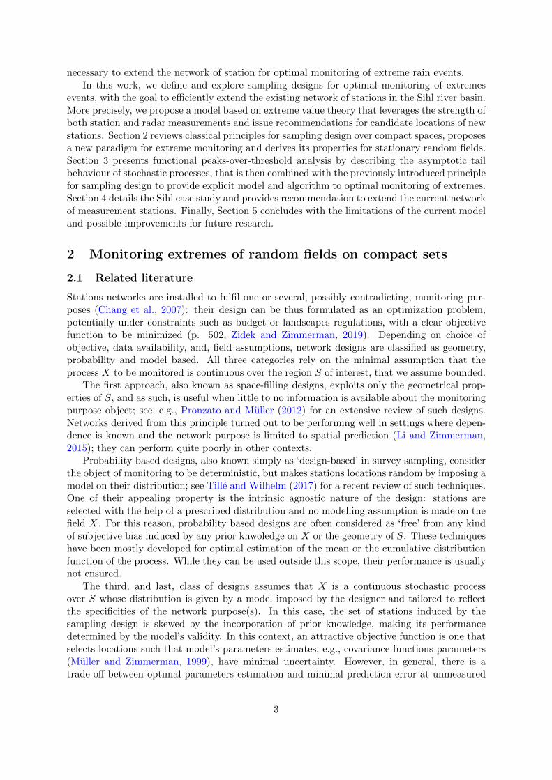
Theorem 1, whose proof can be found in Appendix B, reveals that the supremum of stochasticprocesses is more likely to be located close to the boundary ∂S of S. Such boundary effectinfluences solutions to (3) and, depending of the strength of dependence, favours points on,or close to ∂S. Figure 2 illustrates this phenomenon for two classical models of stochasticprocesses and different level of dependence; see Appendix A for simulation details. We observethat exceedances above the threshold u = 1 are more likely on and close to the boundaries. Wealso note that the boundary effect vanishes as soon as the set Sh reaches a distance greater thanthe dependence range: this phenomenon is observed for the second type a Gaussian processwith weak dependence and, more generally, for any process for which (near)-independence isachieved for large distances. Examining equation (5) in light of Theorem 1 shows a salientaspect of the optimization of sampling designs for monitoring extremes: it yields non-trivialpoints patterns that results from a compromise between a boundary effect and maximizationof inter-location distances.
One way to mitigate the boundary effect is to search for candidate locations not exclusivelywithin S but in a region including S and its extension up to the effective range of dependence
7

Pr
{sup
s∈[0,1]X(s) ≥ 1, sup
s∈[h,h+1]
X(s) ≥ 1
∣∣∣∣∣ sups∈[0,1]
X(s) ≥ 1
}Pr
{sups∈Sh
X(s) ≥ 1, sups∈S\Sh
X(s) < 1
∣∣∣∣∣ sups∈SX(s) > 1
}
0.00
0.25
0.50
0.75
1.00
0 3 6 9h
0.0
0.1
0.2
0.3
−6 −3 0 3 6h
Figure 2: Left: Estimated probabilities of concurrent exceedances as a function of the distanceh for four stationary processes. Right: Estimated probabilities that the process X exceeds1 on the interval Sh = [h − 0.5, h + 0.5] only as a function of its location h ∈ [−5.5, 5.5] inS = [−6, 6] when X satisfies sups∈S X(s) ≥ 1 (right). Estimates are obtained by simulationof Gaussian processes (solid line) and generalize r-Pareto process (dashed lines), for strongdependence (black) and weak dependence (blue).
in all directions. In this case, points inside S are, not surprisingly, systematically favoured asPr {X(s1) ≥ u |sups∈S X(s) ≥ u} in (4) is maximal, and constant, for any s1 ∈ S. In this case,the boundary effect is smoothed but the induced monitoring network is meant to be exposedto false positives. In the absence of boundaries, e.g., if S is a compact manifold, the samplingscheme simply cover the space as well as possible by maximizing the inter-locations distancescorresponding to space-filling points sets, as a consequence of Assumption 1.
We should stress once again that all the previous developments rely on Assumption 1 andsimplification (3), and do not require hypotheses on the asymptotic tail behaviour of the process,as it is commonly done in extreme value theory. Thus, any process whose dependence for finitethreshold u decreases with the distance exhibit such boundary effect. These results howeverrely on strict stationarity, which is unrealistic for most applications. When some a prioriinformation is available, for instance from existing measurement stations, or from other indirectmeasurements, generalized r-Pareto processes can be leveraged to find near-optimal samplingdesigns without assuming strict stationarity.
2.4 Algorithm for optimal sequential sampling design
Solving (1) in its general form is intractable, so in practice we resort to a discretization of theregion of interest. The resolution of the grid is determined by the desired spatial precision of thesolution and the accuracy of the probabilities estimates. Even with such setting, tractabilityof the optimization cannot be ensured when searching for sets of size larger than 3 because ofthe combinatorial nature of the problem. We therefore suggest a sub-optimal, but tractable,method to solve (1), i.e., we propose to search optimal sequential designs using Algorithm 1.This procedure is general, applicable to any risk functional, and for the special case of the
8

Algorithm 1: Sequential algorithm for extremal sampling design.
Input number of location L;Optional: initial set of points Ssamp ;if Ssamp = ∅ then
Choose initial point preferably either at random or using geometrical informationon S;
endfor i from Lsamp + 1 to L do
Solve sadd = arg mins∈S
∣∣Pr {r(X) ≥ u} − Pr{r{s1,...,si−1,s}(X) ≥ u|r(X) ≥ u
}∣∣;Set Ssamp = Ssamp ∪ {sadd}
endreturn Ssamp.
supremum, provides an optimal set of locations as
Pr
{max
s∈{s1,...,sL}X(s) ≥ u
∣∣∣∣ sups∈S
X(s) ≥ u}
= Pr
{max
s∈{s1,...,sL−1}X(s) ≥ u
∣∣∣∣ sups∈S
X(s) ≥ u}
+ Pr(X(sL) ≥ u| sups∈S
X(s) ≥ u)− Pr
(X(sL) ≥ u, max
s∈{s1,...,sL−1}X(s) ≥ u| sup
s∈SX(s) ≥ u
). (6)
Indeed, the first term of the right hand side of (6) is fixed given s1, . . . , sL−1, while the othersdepend only on sL. Thus, sequentially maximizing the left hand side of (6) is equivalent tooptimize the last two terms of the right side, and thus explicitly follows the principles derivedfrom Theorem 1.
Figure 3 illustrates the procedure described in Algorithm 1; in this experiment, probabili-ties are estimated empirically using 106 simulations of a weakly dependent r-generalized Paretoprocess as in Figure 2 and rescaled to 0 and 1 for easier visualization. We consider two initiali-sation: first, two stations located on the boundary of [−6, 6] as prescribed by Theorem 1 and,second, two stations selected at random. In the latter, we observe that, as a consequence of thephenomenon described by Theorem 1, locations on the boundaries are quickly sampled.
In case where the interest lies beyond sequential design, Algorithm 1 can be adapted toinclude a forward-backward steps such has in Zhang (2011). One could also consider k−lookahead strategies, that is the simultaneous inclusion of k measurement stations. In the appli-cation described in Section 4, the implementation of a forward-backward step does not changesignificantly the selected locations.
9

Figure 3: Illustration of Algorithm 1 for sequential addition of 4 locations with boundary(top) and random (bottom) initialization. The curves represent the (conditional) probability ofexceedance and are estimated empirically from 106 simulation of an extremal stationary processsatisfying sups∈[−6,6] x(s) ≥ 1 and scaled to varies between 0 and 1.
3 Extremal sampling designs using extreme value theory
3.1 Peaks-over-threshold analysis
Extreme value theory was first introduced for block maxima, describing the limit distributionof
Mn = maxi=1,...,n
Xi, as n→∞,
where Xi are independent and identically distributed random variables (e.g., Fisher and Tippett,1928; Gnedenko, 1943). However, for more accurate risk quantification and optimal monitoringof extremes toward efficient early warnings of natural disasters, we need to study single eventswith potentially large values, i.e., tail distributions of stochastic processes. For this reason, wefocus on an alternative view on extremes called peaks-over-threshold analysis (Balkema andde Haan, 1974; Pickands, 1975; Davison, 1984).
Let X be a random variable, then for any threshold u < inf{x : F (x) = 1}, under some mildconditions we can find sequences an > 0 and bn such that
nPr
{(1 + ξX−bnan
)1/ξ
+≥ x
}, ξ 6= 0,
nPr
{exp
(X−bnan
)+≥ x
}, ξ = 0,
→ x−1, n→∞, (7)
where (·)+ = max(·, 0) . In practice, (7) means that the conditional distribution of exceedancesover a high threshold can be approximated by a generalized Pareto distribution. The parameterξ, called the tail index, determines the strength of the tail and its support: for ξ > 0, x ≥ uand the tail decay is polynomial (Frechet), for ξ = 0, x ≥ u and the tail has an exponentialdecay (Gumbel), and finally for ξ < 0, x ∈ (u;u− σ/ξ) and we retrieve a polynomial tail decay(Weibull). This result has been generalized to a multivariate setting (Rootzen and Tajvidi, 2006;Rootzen et al., 2018a,b), and more recently to functions (de Fondeville and Davison, 2021).
Again, let S be a compact subset of Rd representing the region under consideration and C(S)denotes the space of real-valued continuous functions over S. We now consider that X refers to
10

a stochastic process with sample path in C(S). In a univariate context, it is straightforward todefine the notion of exceedance, but for functions, it needs to be carefully introduced. FollowingDombry and Ribatet (2015) and de Fondeville and Davison (2018), we consider a functionalr : C(S)→ R, called a risk functional, which computes a univariate summary of the stochasticprocess X and defined an r-exceedance as an event {r(X) > u} where u > 0 is a threshold ofchoice.
We now suppose that there exist sequences of functions an ∈ C(S, (0,∞)) and bn ∈ C(S)and a scalar ξ ∈ R such that
nPr
{(1 + ξ
X − bnan
)1/ξ
∈ ·
}→ Λ(·), (8)
where Λ is a non-degenerate measure on F = C(S, (0,∞)) \ {0}. Equation (8) is a naturalextension of the univariate condition (7) for convergence of the tail distribution towards ageneralized Pareto distribution and implies that
Pr
[X − bnan
∈ (·)∣∣∣∣ r{X − bnan
}> 0
]→ Pr{P ∈ (·)}, n→∞, (9)
where P is a generalized r-Pareto process; detailed conditions on the functional r can be foundin de Fondeville and Davison (2021).
The generalized r-Pareto process P is parametrized by a tail index ξ function and a limitmeasure Λ, respectively characterizing the regime of marginal tail decay and extremal depen-dence. This class of processes is a natural extension of univariate peaks-over-threshold analysisto functions. In particular, for any s ∈ S and sufficiently high threshold u > 0,
Pr{P (s) > u+ x | P (s) > u} = 1− Fξ,σ(u)(x),
where σ(u) = 1+ξu and 1−Fξ,σ(u) is the survival function of a generalized Pareto random vari-able. However, we request that the measure Λ is non-zero on the space of continuous functionson S, which restricts the model to one particular case of extremal dependence, namely asymp-totic dependence. This implies that the strength of the dependence decreases but stabilizes asthe intensity of the event increases, i.e., there exists for each location in s ∈ S a neighbourhoodfor which points are positively associated with X(s) independently of the marginal intensity.
Generalized r-Pareto processes are constructed using the representation
P ={RW/r(W )}ξ − 1
ξ, (10)
where R is a univariate unit Pareto random variable and W is a stochastic process on theunit L1−sphere {x ∈ C(S) : ‖x‖1 = 1} whose distribution is determined by Λ and modelsthe dependence of P . Equation (10) is a key component to sampling algorithms as the onesdescribed in de Fondeville and Davison (2021). In general, the process W can take any kind ofdistribution as soon as E{W (s)} = 1 for all s ∈ S.
Assuming that the tail index ξ is homogeneous over S is common in environmental applica-tions (e.g., Ferreira et al., 2012; Engelke et al., 2019), especially when the region of interest issmall relative to the scale of the process under study. In this case, the tail index ξ characterizesnot local tail behaviors but the tail regime of the physical process itself, e.g., a specfic type ofrainfall. Visual diagnostics, such as qq-plots, allows to assess the reliability of such assumption.In general, the latter can be relaxed, but then, using an asymptotically justified model requiresto define exceedances on the re-normalized process Y = {1 + ξ(X − bn)/an}1/ξ, with the risk tolose any potential physical interpretation.
11

To model extremal dependence, a very convenient model for W is a stationary log-Gaussianrandom field, for which extremal dependence is simply summarized by
ρ(h) = Pr{P (s+ h) > u | P (s) > u} = 2
(1− Φ
[{γ(h)
2
}1/2])
, (11)
where u is a sufficiently large threshold, γ is the semi-variogram of the underlying Gaussianprocess and Φ is the distribution function of a standard normal random variable. The functionρ is called the extremogram (Davis and Mikosch, 2009), or the χ coefficient in a multivariatesetting (Ledford and Tawn, 1996), and measures pairwise extremal dependence. Indeed, forheavy-tailed processes, classical measures of dependence such as a covariance function does notnecessarily exists, and thus we require alternatives such as the extremogram. This model isconvenient as it allows to leverage existing Gaussian dependence models from the literature onspatio-temporal statistics to drive the extremal dependence of P .
In practice, following asymptotic convergence (9), the distribution of functional exceedancescan be approximated by a generalized r-Pareto process, i.e.,
Pr
[X − bnan
∈ ·∣∣∣∣ r{X − bnan
}> 0
]≈ Pr{P ∈ ·} (12)
where the functions an and bn are also unknown and need to be estimated. When the riskfunctional is linear, i.e., the condition in (12) simplifies to exceedances of r(X) above u = bn, alarge n is equivalent to a large threshold u ∈ R. In this case, the random variable r(P ) followsa generalized Pareto distribution with tail index ξ ∈ R, scale an > 0 and location bn ∈ R.
Generalized r-Pareto processes offers a simple and flexible solution to model extremes ofrandom fields. It is the main building block of the methodology proposed here to create, orenlarge, network of monitoring stations, for optimal monitoring of extreme events.
3.2 A flexible model for station networks
We now propose a model to find an optimal sequential sampling design in the sense of (1)when some a priori information of the physical process under consideration is available. Forthe Sihl river, as presented in Section 1, three monitoring stations are installed inside the basinand radar observations cover the whole region, providing information about the intensity andthe structure of extreme rainfall in the region. The goal of such an analysis is to leverage allavailable data and propose guidelines as to where new stations should be installed for optimalmonitoring of extremes.
More precisely, we suppose that, for a risk function r, the distribution of r-exceedances ofthe process X over the threshold u ∈ R can be approximated by a generalized r-Pareto processP as in (12). In this case, the process is allowed to have both non-stationary marginal taildistributions and potentially non-stationary extremal dependence. We also suppose that it ispossible to estimate the parameters of P from the available data, i.e, that we have estimates ofthe functions an, bn, ξ and of the dependence structure of W . In practice, this implies imposinga marginal parametric model such as
an(s) = f{y(s)} > 0,bn(s) = g{y(s)} ∈ R,ξ(s) = ξ ∈ R,
s ∈ S,
where y refers to a vector of covariates, such as locations s ∈ S or any field available throughoutS like altitude or any spatially dense data set such as radar acquisitions. As mentioned in
12

Section 3.1, assuming constant ξ is common in environmental applications and is necessary toensure that the risk can be defined on the original scale. We also suppose that the dependence ofW is parametrized by a vector θW of parameters. For instance, if W is log-Gaussian, θW refersto the parameters of the semi-variogram function γ, which can be allowed to be non-stationaryover space. Estimation procedures for an, bn, ξ and θW can be found in de Fondeville andDavison (2021) .
We also assume that the process X is observed at a set of locations Sobs = {s1, . . . , sLobs} ⊂
S; the latter could be empty if no station measures are available and alternative sources of datacan be leveraged. We denote by Lsamp the number of new sites, i.e., the size of the networkextension. This parameter is usually determined by practical constraints and available budget.With a non-stationary marginal behaviour, and potentially dependence, finding an optimalsampling design is not trivial, so, as in 2.4, we approximate numerically equation (1) with afinite number of potential candidate sites, i.e., we use a grid over S of size Lgrid, whose sizeis determined by the resolution of the covariates y. With this setting, the number of sets ofcandidate sites grows exponentially with Lsamp, getting quickly intractable for Lsamp > 2. Asdetailed in Section 2.4, we propose a sequential procedure to solve (1); this provides a reasonableapproximation of the solution while being computationally efficient. A sequential solution alsoreflects fields practices as in general new weather stations are installed sequentially, as thisis a time consuming and costly process. The procedure is summarized by Algorithm 2 andcombines an empirical estimator of the r-exceedance probabilities with simulations from thefitted generalized r-Pareto process. For the supremum functional, Algorithm 2 provides anexact solution to sequential designs as it was proved in Section 2.4. Note that, for instance, ifthe risk functional is linear and u = r(bn), then we can simply set I = 1, as by definition, allthe elements of the simulation set Pn satisfies r(Pn) ≥ u.
Algorithm 2: Algorithm for near-optimal sequential sampling design to monitor ex-tremes
Input: Sobs, Sgrid, u, an, bn, ξ and θW ;number of desired new sampling points Lsamp, number of simulations N ;Simulate N generalized r-Pareto processes Pn with parameters (ξ, θW );
Compute I = N−1∑N
j=1 1{rSgrid(anPj + bn) ≥ u};
Set Ssamp = ∅;for l from 1 to Lsamp do
for k in 1 to Lgrid do
Set R[k] = |I −N−1∑N
j=1 1{rsk∪Ssamp∪Sobs(anPj + bn) ≥ u}|;
endSet Ssamp = Ssamp ∪ skmax where kmax = arg max
kR[k]
endreturn Ssamp.
4 Optimal network for the Sihl river basin
To study rainfall in the region of Zurich, we can rely on the existing network of weather stations.The Sihl river basin itself contains only three monitoring stations. For improved model inference,we estimate the model using the measurements available in the coloured region in Figure 1,which includes up to 15 monitoring stations. For all these sites, MeteoSwiss provides hourly
13

mean rainfall with measurement from January 1st 2013 to March 2020 for half of them, whilethe 7 others have records starting between 2014 and 2016. Thus the times series have between30000 and 62000 measures. One station outside the river basin has been installed in 2019 andtherefore does not include enough measurements to be safely included.
To estimate a model for a generalized r-Pareto process, we can also leverage radar products.More precisely the CombiPrecip data set (Sideris et al., 2014; Gabella et al., 2017; Panzieraet al., 2018) produced by MeteoSwiss provides estimates of hourly rainfall accumulation since2013 on dense grid of 1km resolution. Earlier measurements are also available but inconsistentwith recent acquisition due to hardware and processing changes in 2013. The Sihl river basinis orographically homogeneous and located at a reasonable distance from the radar, so the es-timated rain fields can be assumed to be fairly homogeneous and free from processing biases.These measures, as the result of some processing, are however not reliable by themselves, i.e.,their link with station measurement is unknown. We however suppose that the radar estimatespresent spatial variations similar to the true underlying rain field. Thus, we use radar mea-surements, first, as covariate to extrapolate the tail marginal model away from existing weatherstations and, second, to estimate the model for extremal dependence.
4.1 Marginal model
In order to use Algorithm 2, we need first to estimate the functions an, bn and the tail indexξ ∈ R. To do so, we assume the following parametric model
an(s) = a ∈ (0,∞),bn(s) = b1 + b2 × y(s),ξ(s) = ξ ∈ R,
s ∈ S, (13)
where y is a covariate derived from radar measurements. This model has been chosen followinga preliminary analysis, where generalized Pareto distributions were fitted independently for eachof the 14 stations and various thresholds: we found both the scale and tail index parameters tobe homogeneous across S and ξ to be stable around quantiles 0.995 of the observational series;this represents between 150 and 300 exceedances per station, and about 2.5% to 5% of wet days.We explored several candidates for the covariate y, including local quantiles at different levels,and average rainfall accumulation, both for wet days only and overall series; we found the later tohave about 95% correlation with empirical 0.995 quantiles from the station measurements. Wethus chose the later as covariate in the parametric model (13); its spatial variation is displayedin Figure 1. Then using a least squares algorithm, we obtain b1 = 1.14(0.34) and b2 = 20.8(2.1);numbers in the brackets refer to estimated standard deviations. The corresponding model bn isdisplayed in Figure 4 and gives values higher than the corresponding empirical quantiles of theradar product. We then use independent likelihood to estimate the common scale a = 1.87(0.05)and tail index ξ = 0.33(0.02). The fit is assessed by visual inspection of the QQ-plots given inAppendix C, which is particularly convincing as it accommodate about 3200 exceedances from14 stations with only 4 parameters. It is not surprising that such a simple model presents agood level of performance as the region under consideration is relatively small, approximately2000km2, with limited variations in altitude and is thus fairly homogeneous from an hydrologicalperspective.
14

Figure 4: Estimated location model bn. The estimate is obtained using a least squares algorithmwith radar based hourly mean rainfall as covariate. The solid black line delimits the Sihl riverbasin and black crosses represent the location of weather stations.
4.2 Dependence model
For generalized r-Pareto processes, extremal dependence is fully characterized by the angularcomponent W , for which we propose to use a log-Gaussian process. More precisely,
W (s) =exp
{G(s)− σ2(s)/2
}‖ exp (G− σ2/2) ‖1
, (14)
where σ2(s) is the variance at location s ∈ S of a zero mean Gaussian process G. We furtherassume that G has stationary increments, i.e., its semi-variogram function γ(s, s′) = var{G(s′)−G(s)} is a function of the distance h = s′−s. We remind that in this case, the pairwise extremaldependence, as summarized by the extremogram, is linked through the closed form (11) to γ,for which we impose parametric model. We choose (Schlather and Moreva, 2017)
γ(h) =(1 + ‖Ah/λ‖α)β/α−1
2β/α − 1(15)
where 0 < α < 2 and β < 2 respectively drive the smoothness and long range behaviour of theprocess, λ > 0 is a scale parameter and A is a geometrical anisotropy matrix
A =
[cos δ − sin δκ sin δ κ cos δ
],
with κ > 0 and δ ∈ (0, π/4). The model (15) is particularly attractive for modelling extremaldependence as, when β < 0, the semi-variogram function is bounded, while when 0 < β < 2,γ(h)→∞ as h→∞, meaning that the process tends to be independent for increasingly largedistances.
The extremogram can be estimated from the observations with
ρ(h) =
∑ni=1 1{Xi(s+ h) ≥ uq(s+ h), Xi(s) ≥ uq(s)}
1{∑n
i=1Xi(s) ≥ uq(s)}(16)
where uq(s) is the qth quantile of X at location s, q ∈ (0, 1) close enough to 1. We apply equation(16) on radar rainfall measurements with quantile level q = 0.995. We then fit a parametricmodel for the semi-variogram function γ using a least squares procedure.
15

Empirical Estimates Fitted Model
Figure 5: Empirical (left) and modelled (right) pairwise dependence estimated from radarrainfall measurements.
Figure 5 displays the empirical estimates against the estimated model. We observe a ratherstrong dependence up to 20km especially in the north-west direction, which drops quite quicklyafter 25km. These estimates are consistent with the observation that at such a fine scale, rainfallevents tends to be localized in regions with diameters of no more than few dozens of kilometers.
4.3 New measurement stations in the Sihl Basin
Algorithm 2 relies on the generation of large samples of generalized r-Pareto processes, i.e., sim-ulations of the angular component W , for which a detailed algorithm can be found in AppendixD. The model’s output for the risk functional r(X) = sups∈S X(s) with threshold u = 20mmand 105 simulations are displayed in Figure 6 for sequential extensions by 10 and 20 stations.
We also observe that as the number of sites increases, recommended locations tend to belocated on the boundaries of the region, consistently with the results of Section 2.3. The veryfirst station to be added is located in Zurich at the train station, however its relevance is limitedas a station is already installed few kilometers away from the recommended location, as it canbe seen in the Figure 1. The algorithm could be adapted to account for this phenomenon byextending the region by a few kilometers in all directions, mitigating the boundary effect butallowing for false positive when the network is used for early warning. The Sihl river basin alsoincludes three stations that are manually operated by MeteoSwiss but can unfortunately notbe leveraged for statistical analysis due to the temporal irregularity of the measurements. InFigure 6, we can see that Algorithm 2 suggests to automate one of them for the 20 stationsscenario.
16

Figure 6: Locations of 10 (left) and 20 (right) new weather stations for optimal monitoringof extreme rainfall inside the Sihl river basin with sequential sampling designs. Blue crosses:Existing stations; blue dots: new stations; plain red line: basin limit; green triangles: existingmanual measurements stations.
5 Discussion
In this work, we propose a new principle for sampling designs aiming to achieve optimal mon-itoring of extremes. We study the theoretical properties of the induced point patterns whenmonitoring the supremum of stationary stochastic processes whose dependence is assumed todecrease with distance. We obtain sampling designs resulting from a compromise betweeninter-location distance maximization and a boundary effect whose influence is determined bythe strength of dependence. We also propose a tractable algorithm, relying on sequential de-signs, to approximate our criterion for optimal sampling. When data is available in the region ofinterest, as it is the case of Sihl river basin, we propose a model, based on generalized r-Paretoprocesses, allowing us to propose recommendations for possibly extending the existing networkby 10 and 20 stations.
Compared to other approaches, such as Gaussian processes, the proposed methodologyallows a principled modelization of the tail of distribution, by using an asymptotically justifiedframework. The dependence structure that can be modelled is quite flexible, and could be madenon-stationary using techniques such as Fuglstad et al. (2015) or Fouedjio et al. (2015), whena sufficiently large number of stations is already in operation. Our procedure can be efficientlyimplemented using the algorithm described in the Section 2.4. This contribution should alsoprove to be useful in a wide variety of settings. For instance, Chang et al. (2007), due to theabsence of better and more specialized alternatives, resorted to use a multivariate Gaussian-Inverse Wishart hierarchical Bayesian distribution to monitor air pollution. However, as theysay, “the primary role – of air pollution monitoring networks – is the detection of noncompliancewith air quality standards based on extremes designed to protect human health”, and thus ourmodel, which is tailored for extremes monitoring, would be particularly relevant in this context.
Finally, the proposed model for the Sihl river relies on generalized r-Pareto processes, forwhich the strength of extremal dependence is ‘frozen’ above a given level of intensity: themodel is thus conservative by nature and extremal dependence might be over-estimated above
17

the quantile of reference. Asymptotic models cannot accommodate for decreasing trends ofdependence with intensity that is observed in multiple environmental applications and sub-asymptotic alternatives for functional peaks-over-threshold should then be considered. However,only very few of them exists (Davison and Gholamrezaee, 2012; Huser et al., 2017; Huser andWadsworth, 2019) and would either not be tractable or sufficiently realistic in the applicationconsidered in this work.
References
Adler, R. J. and Taylor, J. E. (2007). Random Fields and Geometry. Springer, New-York.
Arnaud, A., Bect, J., Couplet, M., Pasanisi, A., and Vazquez, E. (2010). Evaluation d’unRisque d’Inondation Fluviale par Planification Sequentielle d’Experiences. In compte-rendusdes 42emes Journees de Statistique.
Azzimonti, D., Bect, J., Chevalier, C., and Ginsbourger, D. (2016). Quantifying Uncertaintieson Excursion Sets Under a Gaussian Random Field Prior. SIAM-ASA Journal on UncertaintyQuantification, 4(1):850–874.
Azzimonti, D., Ginsbourger, D., Chevalier, C., Bect, J., and Richet, Y. (2019a). Adaptive Designof Experiments for Conservative Estimation of Excursion Sets. Technometrics, 63(1):13–26.
Azzimonti, D., Ginsbourger, D., Rohmer, J., and Idier, D. (2019b). Profile Extrema for Visual-izing and Quantifying Uncertainties on Excursion Regions: Application to Coastal Flooding.Technometrics, 61(4):474–493.
Balkema, A. A. and de Haan, L. (1974). Residual Life Time at Great Age. The Annals ofApplied Statistics, 2(5):792–804.
Bect, J., Ginsbourger, D., Li, L., Picheny, V., and Vazquez, E. (2012). Sequential Designof Computer Experiments for the Estimation of a Probability of Failure. Statistics andComputing, 22(3):773–793.
Bezzola, G. R. and Hegg, C. (2007). Ereignisanalyse Hochwasser 2005, Teil 1 - Prozessse,Schaden und erste Einordnung. Technical report, Bundesamt fur Umwelt und EidgenossicheForschungsanstalt fur Wald, Schnee und Landschaft (WSL).
Chang, H., Fu, A. Q., Le, N. D., and Zidek, J. V. (2007). Designing Environmental MonitoringNetworks to Measure Extremes. Environmental and Ecological Statistics, 14(3):301–321.
Chevalier, C., Ginsbourger, D., Picheny, V., Bect, J., Vazquez, E., and Richet, Y. (2014). FastParallel Kriging-Based Stepwise Uncertainty Reduction With Application to the Identificationof an Excursion Set. Technometrics, 56(4):455–465.
Cloke, H. L. and Pappenberger, F. (2009). Ensemble Flood Forecasting: a Review. Journal ofHydrology, 375(3-4):613–626.
Davis, R. A. and Mikosch, T. (2009). The Extremogram: a Correlogram for Extreme Events.Bernoulli, 15(4):977–1009.
Davison, A. C. (1984). Modelling Excesses over High Thresholds, with an Application. Inde Oliveira, J. T., editor, Statistical Extremes and Applications, pages 461–482. Reidel, Dor-drecht.
18

Davison, A. C. and Gholamrezaee, M. M. (2012). Geostatistics of Extremes. Proceedings of theRoyal Society A: Mathematical, Physical and Engineering Sciences, 468(2138):581–608.
de Fondeville, R. and Davison, A. C. (2018). High-dimensional Peaks-over-threshold Inference.Biometrika, 105(3):575–592.
de Fondeville, R. and Davison, A. C. (2021). Functional Peaks-over-threshold Analysis.arXiv:2002.02711.
Dombry, C. and Ribatet, M. (2015). Functional Regular Variations, Pareto Processes and PeaksOver Thresholds. Statistics and Its Interface, 8(1):9–17.
Engelke, S., de Fondeville, R., and Oesting, M. (2019). Extremal Behaviour of Aggregated Datawith an Application to Downscaling. Biometrika, 106(1):127–144.
Ferreira, A., de Haan, L., and Zhou, C. (2012). Exceedance Probability of the Integral of aStochastic Process. Journal of Multivariate Analysis, 105(1):241–257.
Fisher, R. A. and Tippett, L. H. C. (1928). Limiting Forms of the Frequency Fistribution ofthe Largest or Smallest Member of a Sample. Mathematical Proceedings of the CambridgePhilosophical Society, 24(2):180–190.
Fouedjio, F., Desassis, N., and Romary, T. (2015). Estimation of space deformation model fornon-stationary random functions. Spatial Statistics, 13:45–61.
Fuglstad, G.-A., Lindgren, F., Simpson, D., and Rue, H. (2015). Exploring a New Class ofNon-stationary Spatial Gaussian Random Fields with Varying Local Anisotropy. StatisticaSinica, 25(1):115–133.
Furrer, E. M. and Katz, R. W. (2008). Improving the Simulation of Extreme PrecipitationEvents by Stochastic Weather Generators. Water Resources Research, 44(12):1–13.
Gabella, M., Speirs, P., Hamann, U., Germann, U., and Berne, A. (2017). Measurement of Pre-cipitation in the Alps Using Dual-polarization C-Band Ground-based Radars, the GPMSpace-borne Ku-Band Radar, and Rain Gauges. Remote Sensing, 9(11):1147–1166.
Gnedenko, B. (1943). Sur la Distribution Limite du Terme Maximum d’une Serie Aleatoire.Annals of Mathematics, 44(3):423–453.
Hainy, M., Muller, W. G., and Wagner, H. (2016). Likelihood-free Simulation-based OptimalDesign with an Application to spatial extremes. Stochastic Environmental Research and RiskAssessment, 30(2):481–492.
Huser, R., Opitz, T., and Thibaud, E. (2017). Bridging Asymptotic Independence and Depen-dence in Spatial Extremes Using Gaussian Scale Mixtures. Spatial Statistics, 21(1):166–186.
Huser, R. and Wadsworth, J. L. (2019). Modeling Spatial Processes with Unknown ExtremalDependence Class. Journal of the American Statistical Association, 114(525):434–444.
Jones, D. R., Schonlau, M., and Welch, W. J. (1998). Efficient Global Optimization of ExpensiveBlack-Box Functions. Journal of Global Optimimisation, 13(4):455–492.
Ledford, A. W. and Tawn, J. A. (1996). Statistics for Near Independence in MultivariateExtreme Values. Biometrika, 83(1):169–187.
19

Li, J. and Zimmerman, D. L. (2015). Model-based Sampling Design for Multivariate Geostatis-tics. Technometrics, 57(1):75–86.
Muller, W. G. and Zimmerman, D. L. (1999). Optimal Designs for Variogram Estimation.Environmetrics, 10(1):23–37.
Panziera, L., Gabella, M., Germann, U., and Martius, O. (2018). A 12-year Radar-basedClimatology of Daily and Sub-daily Extreme Precipitation over the Swiss Alps. InternationalJournal of Climatology, 38(10):3749–3769.
Pickands, J. (1975). Statistical Inference using Extreme Order Statistics. The Annals of Statis-tics, 3(1):119–131.
Pronzato, L. and Muller, W. G. (2012). Design of Computer Experiments : Space Filling andBeyond. Statistics and Computing, 22(1):681–701.
Pukelsheim, F. (2006). Optimal Design of Experiments. Society for Industrial and AppliedMathematics (SIAM), Philadelphia.
Rootzen, H., Segers, J., and Wadsworth, J. L. (2018a). Multivariate Generalized Pareto Distri-butions: Parametrizations, Representations, and Properties. Journal of Multivariate Analy-sis, 165(1):117–131.
Rootzen, H., Segers, J., and Wadsworth, J. L. (2018b). Multivariate Peaks-over-thresholdsModels. Extremes, 21(1):115–145.
Rootzen, H. and Tajvidi, N. (2006). Multivariate Generalized Pareto Distributions. Bernoulli,12(5):917–930.
Santner, T. J., Williams, B. J., and Notz, W. I. (2018). The Design and Analysis of ComputerExperiments. Springer, New York, second edition.
Schlather, M. and Moreva, O. (2017). A Parametric Model Bridging Between Bounded andUnbounded Variograms. Stat, 6(1):47–52.
Sideris, I. V., Gabella, M., Erdin, R., and Germann, U. (2014). Real-time Radar-rain-gaugeMerging Using Spatio-temporal Co-kriging with External Drift in the Alpine Terrain ofSwitzerland. Quarterly Journal of the Royal Meteorological Society, 140(680):1097–1111.
Tille, Y. and Wilhelm, M. (2017). Probability Sampling Designs: Principles for Choice of Designand Balancing. Statistical Science, 32(2):176–189.
Tobler, W. . R. . (1970). A Computer Movie Simulating Urban Growth in the Detroit. EconomicGeography, 46(suppl):234–240.
Wang, Y. and Stoev, S. A. (2013). Conditional Sampling for Spectrally Discrete Max-stableRandom Field. Advances in Applied Probability, 43(2):461–483.
Zhang, T. (2011). Adaptive Forward-backward Greedy Algorithm for Learning Sparse Repre-sentations. IEEE Transactions on Information Theory, 57(7):4689–4708.
Zidek, J. V. and Zimmerman, D. L. (2019). Monitoring Network Design. In Gelfand, A.,Fuentes, M., Hoeting, J. A., and Smith, R. L., editors, Handbook of Environmental andEcological Statistics, pages 499 – 522. CRC Press, Boca Raton.
20

A Simulation parameters for Figure 2
In Figure 2, estimates are obtained by estimating of empirical probabilities using 1000 samples ofeach processes. The procedure in repeated 1000 times to also obtain 95% confidences intervals.Both Gaussian and generalized r-Pareto processes are defined on S = [−6; 6] and simulatedover a regular grid with lag 0.1. For the Gaussian processes, we use semi-variogram function
γG(h) = σ[1− exp{(h/λ)α}], h > 0,
with σ = 2, α = 1.5, λ = 100 for the strong dependence case and λ = 1 for the weakly dependentcase. Generalized r-Pareto processes are constructed using model (14), for which we use:
• for the strong dependence case,
γW (h) = σ[1− exp{(h/λ)α}], h > 0,
with σ = 2, α = 1.5, and λ = 10;
• for the weak dependence case,
γW (h) = (h/λ)α, h > 0
with α = 1.5, and λ = 2.5.
B Proof of Theorem 1
Suppose that X is a stationary process on C(Rd) with d > 0. For simplicity, we prove Theorem1 for d = 1 but generalization to d > 1 is can be done using similar arguments. We study thecompact subset [0, S] with S > 0 and let s ∈ [0, S] and consider a threshold u ∈ R such thatPr{X(s) ≥ u} > 0. Let h ∈ H =]0, S − s] and define the function µ : H → R such that
µ(h) = Pr{ sups∈[h,s+h]
X(s) ≥ u, sups∈[0,S]\[h,s+h]
X(s) < u}
= Pr{ sups∈[h,s+h]
X(s) ≥ u} − Pr{ sups∈[h,s+h]
X(s) ≥ u, sups∈[0,S]\[h,s+h]
X(s) ≥ u}
and we aim to prove that µ(h) is decreasing if h < (S − s)/2 and increasing when h > (S −s)/2, i.e., µ(h) is a decreasing function of the distance to the boundaries of d([h, h + s], ∂S) =infs∈[h,h+s] infs′∈∂S d(s, s′).
For any h′ ∈ [0, S−(s+h)2 ], using the stationarity of X, we have
µ(h+ h′) = Pr{ sups∈[h+h′,s+h+h′]
X(s) ≥ u, sups∈[0,S]\[h+h′,s+h+h′]
X(s) ≤ u},
= Pr{ sups∈[h,s+h]
X(s) ≥ u, sups∈[−h′,S−h′]\[h,s+h]
X(s) ≤ u},
= Pr{ sups∈[h,s+h]
X(s) ≥ u, sups∈[−h′,0]\[h,s+h]
X(s) ≤ u, sups∈[0,S−h′]\[h,s+h]
X(s) ≤ u},
= Pr{A(h, h′), sups∈[−h′,0]\[h,s+h]
X(s) ≤ u},
= Pr{A(h, h′)} − Pr{A(h, h′), sups∈[−h′,0]
X(s) ≥ u}
21

where A(h, h′) = {sups∈[h,s+h]X(s) ≥ u, sup[0,S−h′]\[h,s+h]X(s) ≤ u}. Similarly, we have
µ(h) = Pr{A(h, h′)} − Pr{A(h, h′), sups∈[S−h′,S]
X(s) ≥ u}.
|−h′
|0
|h
| |S − h′
|S
|s+ h
//// ////////////// ///////////////////// //////////////
The difference µ(h+ h′)− µ(h) is thus
µ(h+ h′)− µ(h) = Pr{ sup[0,S−h′]\[h,s+h]
X(s) ≤ u, sups∈[h,s+h]
X(s) ≥ u, sups∈[S−h′,S]
X(s) ≥ u}
− Pr{ sup[0,S−h′]\[h,s+h]
X(s) ≤ u, sups∈[h,s+h]
X(s) ≥ u, sups∈[−h′,0]
X(s) ≥ u}
The condition sup[0,S−h′]\[h,s+h]X(s) ≤ u defines a hitting scenario H1 for which X exceeds uexclusively on [h, s+ h] and [−h′, 0]. Following Assumption 1, we have
Pr{ sups∈[h,s+h]
X(s) ≥ u, sups∈[S−h′,S]
X(s) ≥ u,H1} ≥ Pr{ sups∈[h,s+h]
X(s) ≥ u, sups∈[−h′,0]
X(s) ≥ u,H1}
(17)if
dist([h, s+ h], [−h′, 0]) = h > dist([h, s+ h], [S − h′, S]) = S − h′ − (s+ h),
or equivalently if h > (S−h′− s)/2. Inequality (17) is reversed when h < (S−h′− s)/2, whichconcludes the proof of Theorem 1.
C Qq-plots for the station tail distributions
22

5 10 15 20 25 30 35
020
4060
8010
0
Cham
modelQuantiles
exce
sses
Sor
ted
−−−−−−−−−−−−−−−−−−−−−−−−−−−−−−−−−−−−−−−−−−−−−−−−−−−−−−−−−−−−−−−−−−−−−−−−−−−−−−−−−−−−−−−−−−−−−−−−−−−−−−−−−−−−−−−−−−−−−−−−−−−−−−−−−−−−−−−−−−−−−−−−−−−−−−−−−−−−−−−−−−−−−−−−−−−−−−−−−−−−−−−−−−−−−−−−−−−−−−−−−−−−−−−−−−
−−−−−−−−−−−−−−−−−−−−−−−−−−−−−−−−−−−−−
−−−−−−−−−−−
−−−−−− − −−
−−
−
−
−
−−−−−−−−−−−−−−−−−−−−−−−−−−−−−−−−−−−−−−−−−−−−−−−−−−−−−−−−−−−−−−−−−−−−−−−−−−−−−−−−−−−−−−−−−−−−−−−−−−−−−−−−−−−−−−−−−−−−−−−−−−−−−−−−−−−−−−−−−−−−−−−−−−−−−−−−−−−−−−−−−−−−−−−−−−−−−−−−−−−−−−−−−−−−−−−−−−−−−−−−−−−−−−−−−−−−−−−−−−−−−−−−−−−−−−−−−−
−−−−−−−−−−−−−−−−−−−−−−−−−−−−−− − − − − − − −
−
5 10 15 20 25 30 35
020
4060
8010
012
0
Einsiedeln
modelQuantiles
exce
sses
Sor
ted
−−−−−−−−−−−−−−−−−−−−−−−−−−−−−−−−−−−−−−−−−−−−−−−−−−−−−−−−−−−−−−−−−−−−−−−−−−−−−−−−−−−−−−−−−−−−−−−−−−−−−−−−−−−−−−−−−−−−−−−−−−−−−−−−−−−−−−−−−−−−−−−−−−−−−−−−−−−−−−−−−−−−−−−−−−−−−−−−−−−−−−−−−−−−−−−−−−−−−−−−−−−−−−−−−−−−−−−−−−−−−−−−−−−−−−−−−−−−−−−−−−−−−−−−−−
−−−−−−−−−−−−−−−−−−−−−−−−−−−−−−−−−−−−−
−−−−−−−−−−−−−−− −
− −−
−
−
−
−−−−−−−−−−−−−−−−−−−−−−−−−−−−−−−−−−−−−−−−−−−−−−−−−−−−−−−−−−−−−−−−−−−−−−−−−−−−−−−−−−−−−−−−−−−−−−−−−−−−−−−−−−−−−−−−−−−−−−−−−−−−−−−−−−−−−−−−−−−−−−−−−−−−−−−−−−−−−−−−−−−−−−−−−−−−−−−−−−−−−−−−−−−−−−−−−−−−−−−−−−−−−−−−−−−−−−−−−−−−−−−−−−−−−−−−−−−−−−−−−−−−−−−−−−−−−−−−−−−−−−−−−−−−−−−−−−−
−−−−−−−−−−−−−−−−−−−−−−−−−−− − − − − − −
−
5 10 15 20 25 30 35
2040
6080
100
Innerthal
modelQuantiles
exce
sses
Sor
ted
−−−−−−−−−−−−−−−−−−−−−−−−−−−−−−−−−−−−−−−−−−−−−−−−−−−−−−−−−−−−−−−−−−−−−−−−−−−−−−−−−−−−−−−−−−−−−−−−−−−−−−−−−−−−−−−−−−−−−−−−−−−−−−−−−−−−−−−−−−−−−−−−−−−−−−−−−−−−−−−−−−−−−−−−−−−−−−−−−−−−−−−−−−−−
−−−−−−−−−−−−−−−−−−−−−−−−−−−−−−−−−−−
−−−−−−−−−−−−
−−−− − −−
−−
−
−
−
−−−−−−−−−−−−−−−−−−−−−−−−−−−−−−−−−−−−−−−−−−−−−−−−−−−−−−−−−−−−−−−−−−−−−−−−−−−−−−−−−−−−−−−−−−−−−−−−−−−−−−−−−−−−−−−−−−−−−−−−−−−−−−−−−−−−−−−−−−−−−−−−−−−−−−−−−−−−−−−−−−−−−−−−−−−−−−−−−−−−−−−−−−−−−−−−−−−−−−−−−−−−−−−−−−−−−
−−−−−−−−−−−−−−−−−−−−−−−−−− − − − − − − −
−
5 10 15 20 25
2040
6080
Jona
modelQuantiles
exce
sses
Sor
ted
−−−−−−−−−−−−−−−−−−−−−−−−−−−−−−−−−−−−−−−−−−−−−−−−−−−−−−−−−−−−−−−−−−−−−−−−−−−−−−−−−−−−−−−−−−−−−−−−−−−−−−−−
−−−−−−−−−−−−−−−−−−−−−−−−−−−
−−−−−−−−−−−−
− −−
−−
−
−
−
−−−−−−−−−−−−−−−−−−−−−−−−−−−−−−−−−−−−−−−−−−−−−−−−−−−−−−−−−−−−−−−−−−−−−−−−−−−−−−−−−−−−−−−−−−−−−−−−−−−−−−−−−−−−−−−−−−−−−−−−−−−−−
−−−−−−−−−−−−−−−−−− − − − − − − −
−
5 10 15 20 25 30
2040
6080
100
Lachen / Galgenen
modelQuantiles
exce
sses
Sor
ted
−−−−−−−−−−−−−−−−−−−−−−−−−−−−−−−−−−−−−−−−−−−−−−−−−−−−−−−−−−−−−−−−−−−−−−−−−−−−−−−−−−−−−−−−−−−−−−−−−−−−−−−−−−−−−−−−−−−−−−−−−−−−−−−−−−−−−−−
−−−−−−−−−−−−−−−−−−−−−−−−−−−−
−−−−−−−−−−−− − −
−−
−
−
−
−
−−−−−−−−−−−−−−−−−−−−−−−−−−−−−−−−−−−−−−−−−−−−−−−−−−−−−−−−−−−−−−−−−−−−−−−−−−−−−−−−−−−−−−−−−−−−−−−−−−−−−−−−−−−−−−−−−−−−−−−−−−−−−−−−−−−−−−−−−−−−−−−−−−−−−−−−−−−−
−−−−−−−−−−−−−−−−−−− − − − − − − −
−
5 10 15 20 25 30
2040
6080
100
Oberiberg
modelQuantiles
exce
sses
Sor
ted
−−−−−−−−−−−−−−−−−−−−−−−−−−−−−−−−−−−−−−−−−−−−−−−−−−−−−−−−−−−−−−−−−−−−−−−−−−−−−−−−−−−−−−−−−−−−−−−−−−−−−−−−−−−−−−−−−−−−−−−−−
−−−−−−−−−−−−−−−−−−−−−−−−−
−−−−−−−−− − −
−−
−
−
−
−
−−−−−−−−−−−−−−−−−−−−−−−−−−−−−−−−−−−−−−−−−−−−−−−−−−−−−−−−−−−−−−−−−−−−−−−−−−−−−−−−−−−−−−−−−−−−−−−−−−−−−−−−−−−−−−−−−−−−−−−−−−−−−−−−−−−−−−−−−−−−
−−−−−−−−−−−−−−− − − − − − − −−
Figure 7: QQ-plot of the fitted model for the tail distribution of the 6 first, out of 14, stationsused in the analysis with 95% confidence intervals obtained by parametric bootstrap.
23

5 10 15 20 25 30
2040
6080
100
Rempen
modelQuantiles
exce
sses
Sor
ted
−−−−−−−−−−−−−−−−−−−−−−−−−−−−−−−−−−−−−−−−−−−−−−−−−−−−−−−−−−−−−−−−−−−−−−−−−−−−−−−−−−−−−−−−−−−−−−−−−−−−−−−−−−−−−−−−−−−−−−−−−−−−−−−−−−−−−−−
−−−−−−−−−−−−−−−−−−−−−−−−−−
−−−−−−−−− − − −
−−
−
−
−
−−−−−−−−−−−−−−−−−−−−−−−−−−−−−−−−−−−−−−−−−−−−−−−−−−−−−−−−−−−−−−−−−−−−−−−−−−−−−−−−−−−−−−−−−−−−−−−−−−−−−−−−−−−−−−−−−−−−−−−−−−−−−−−−−−−−−−−−−−−−−−−−−−−−−−−−−−
−−−−−−−−−−−−−−−− − − − − − − −−
5 10 15 20 25 30 35 40
020
4060
8010
012
014
0
Rossberg
modelQuantiles
exce
sses
Sor
ted
−−−−−−−−−−−−−−−−−−−−−−−−−−−−−−−−−−−−−−−−−−−−−−−−−−−−−−−−−−−−−−−−−−−−−−−−−−−−−−−−−−−−−−−−−−−−−−−−−−−−−−−−−−−−−−−−−−−−−−−−−−−−−−−−−−−−−−−−−−−−−−−−−−−−−−−−−−−−−−−−−−−−−−−−−−−−−−−−−−−−−−−−−−−−−−−−−−−−−−−−−−−−−−−−−−−−−−−−−−−−−−−−−−−−−−−−−−−−−−−−−−−−−−−−−−−−−−−−−−−−−−−−−−−−−−−−−−−−−−−−−−−−−−−−−−−−−−−−−−−−−−−−−−−−
−−−−−−−−−−−−−−−−−−−−−−−−−−−−−−−−−−−−−
−−−−−−−−−−−−− −
− −−
−
−
−
−−−−−−−−−−−−−−−−−−−−−−−−−−−−−−−−−−−−−−−−−−−−−−−−−−−−−−−−−−−−−−−−−−−−−−−−−−−−−−−−−−−−−−−−−−−−−−−−−−−−−−−−−−−−−−−−−−−−−−−−−−−−−−−−−−−−−−−−−−−−−−−−−−−−−−−−−−−−−−−−−−−−−−−−−−−−−−−−−−−−−−−−−−−−−−−−−−−−−−−−−−−−−−−−−−−−−−−−−−−−−−−−−−−−−−−−−−−−−−−−−−−−−−−−−−−−−−−−−−−−−−−−−−−−−−−−−−−−−−−−−−−−−−−−−−−−−−−−−−−−−−−−−−−−−−−−−−−−−−−−−−−−−−−−−−−−
−−−−−−−−−−−−−−−−−−−−−−−−−− − − − − − −
−
5 10 15 20 25 30 35
020
4060
8010
012
0
Sattel, SZ
modelQuantiles
exce
sses
Sor
ted
−−−−−−−−−−−−−−−−−−−−−−−−−−−−−−−−−−−−−−−−−−−−−−−−−−−−−−−−−−−−−−−−−−−−−−−−−−−−−−−−−−−−−−−−−−−−−−−−−−−−−−−−−−−−−−−−−−−−−−−−−−−−−−−−−−−−−−−−−−−−−−−−−−−−−−−−−−−−−−−−−−−−−−−−−−−−−−−−−−−−−−−−−−−−−−−−−−−−−−−−−−−−−−−−−−−−−−−−−−−−−−−−−−−−−−−−−−−−−−−−−−
−−−−−−−−−−−−−−−−−−−−−−−−−−−−−−−−−−−−−−
−−−−−−−−−−−
−−−− − −−
−−
−
−
−
−−−−−−−−−−−−−−−−−−−−−−−−−−−−−−−−−−−−−−−−−−−−−−−−−−−−−−−−−−−−−−−−−−−−−−−−−−−−−−−−−−−−−−−−−−−−−−−−−−−−−−−−−−−−−−−−−−−−−−−−−−−−−−−−−−−−−−−−−−−−−−−−−−−−−−−−−−−−−−−−−−−−−−−−−−−−−−−−−−−−−−−−−−−−−−−−−−−−−−−−−−−−−−−−−−−−−−−−−−−−−−−−−−−−−−−−−−−−−−−−−−−−−−−−−−−−−−−−−−−−−−−−−−
−−−−−−−−−−−−−−−−−−−−−−−−−−−−− − − − − − − −
−
5 10 15 20 25 30
2040
6080
100
Siebnen
modelQuantiles
exce
sses
Sor
ted
−−−−−−−−−−−−−−−−−−−−−−−−−−−−−−−−−−−−−−−−−−−−−−−−−−−−−−−−−−−−−−−−−−−−−−−−−−−−−−−−−−−−−−−−−−−−−−−−−−−−−−−−−−−−−−−−−−−−−−−−−−−−−−−−−−−−−−−−−−
−−−−−−−−−−−−−−−−−−−−−−−−−−−−
−−−−−−−−−−−− − − −
−−
−
−
−
−−−−−−−−−−−−−−−−−−−−−−−−−−−−−−−−−−−−−−−−−−−−−−−−−−−−−−−−−−−−−−−−−−−−−−−−−−−−−−−−−−−−−−−−−−−−−−−−−−−−−−−−−−−−−−−−−−−−−−−−−−−−−−−−−−−−−−−−−−−−−−−−−−−−−−−−−−−−−−−
−−−−−−−−−−−−−−−−−−− − − − − − − −
−
5 10 15 20 25 30
020
4060
8010
0
Sihlbrugg
modelQuantiles
exce
sses
Sor
ted
−−−−−−−−−−−−−−−−−−−−−−−−−−−−−−−−−−−−−−−−−−−−−−−−−−−−−−−−−−−−−−−−−−−−−−−−−−−−−−−−−−−−−−−−−−−−−−−−−−−−−−−−−−−−−−−−−−−−−−−−−−−−−−−−−−−−−−−−−−−−−−−−−−−−−−−−−−−−−−−−−−−−−−−−−−−
−−−−−−−−−−−−−−−−−−−−−−−−−−−−−
−−−−−−−−−−−−− − −
−−
−
−
−
−
−−−−−−−−−−−−−−−−−−−−−−−−−−−−−−−−−−−−−−−−−−−−−−−−−−−−−−−−−−−−−−−−−−−−−−−−−−−−−−−−−−−−−−−−−−−−−−−−−−−−−−−−−−−−−−−−−−−−−−−−−−−−−−−−−−−−−−−−−−−−−−−−−−−−−−−−−−−−−−−−−−−−−−−−−−−−−−−−−−−−−−−−−−−−−−−−
−−−−−−−−−−−−−−−−−−−−− − − − − − − −
−
5 10 15 20 25 30 35 40
020
4060
8010
012
0
Wädenswil
modelQuantiles
exce
sses
Sor
ted
−−−−−−−−−−−−−−−−−−−−−−−−−−−−−−−−−−−−−−−−−−−−−−−−−−−−−−−−−−−−−−−−−−−−−−−−−−−−−−−−−−−−−−−−−−−−−−−−−−−−−−−−−−−−−−−−−−−−−−−−−−−−−−−−−−−−−−−−−−−−−−−−−−−−−−−−−−−−−−−−−−−−−−−−−−−−−−−−−−−−−−−−−−−−−−−−−−−−−−−−−−−−−−−−−−−−−−−−−−−−−−−−−−−−−−−−−−−−−−−−−−−−−−−−−−−−−−−−−−−−−−−−−−−−−−−−−−−−−−−−−−−−−−−−−−−−−−−−−−−−−
−−−−−−−−−−−−−−−−−−−−−−−−−−−−−−−−−−−−−−−−−
−−−−−−−−−−−−−−−− − −
−−
−
−
−
−−−−−−−−−−−−−−−−−−−−−−−−−−−−−−−−−−−−−−−−−−−−−−−−−−−−−−−−−−−−−−−−−−−−−−−−−−−−−−−−−−−−−−−−−−−−−−−−−−−−−−−−−−−−−−−−−−−−−−−−−−−−−−−−−−−−−−−−−−−−−−−−−−−−−−−−−−−−−−−−−−−−−−−−−−−−−−−−−−−−−−−−−−−−−−−−−−−−−−−−−−−−−−−−−−−−−−−−−−−−−−−−−−−−−−−−−−−−−−−−−−−−−−−−−−−−−−−−−−−−−−−−−−−−−−−−−−−−−−−−−−−−−−−−−−−−−−−−−−−−−−−−−−−−−−−−−−−−−−−−−−−−−−−−
−−−−−−−−−−−−−−−−−−−−−−−−−−−−−− − − − − − −
−
Figure 8: QQ-plot of the fitted model for the tail distribution of stations 7 to 12 used in theanalysis with 95% confidence intervals obtained by parametric bootstrap.
24

5 10 15 20 25
020
4060
80
Zwillikon
modelQuantiles
exce
sses
Sor
ted
−−−−−−−−−−−−−−−−−−−−−−−−−−−−−−−−−−−−−−−−−−−−−−−−−−−−−−−−−−−−−−−−−−−−−−−−−−−−−−−−−−−−−−−−−−−−−−−−−−−−−
−−−−−−−−−−−−−−−−−−−−−−−−
−−−−−−−−−−− − − −
−−
−
−
−
−−−−−−−−−−−−−−−−−−−−−−−−−−−−−−−−−−−−−−−−−−−−−−−−−−−−−−−−−−−−−−−−−−−−−−−−−−−−−−−−−−−−−−−−−−−−−−−−−−−−−−−−−−−−−−−−−−−−−−−−
−−−−−−−−−−−−−−−− − − − − − − −−
5 10 15 20 25 30 35
020
4060
8010
012
0
Zürich / Fluntern
modelQuantiles
exce
sses
Sor
ted
−−−−−−−−−−−−−−−−−−−−−−−−−−−−−−−−−−−−−−−−−−−−−−−−−−−−−−−−−−−−−−−−−−−−−−−−−−−−−−−−−−−−−−−−−−−−−−−−−−−−−−−−−−−−−−−−−−−−−−−−−−−−−−−−−−−−−−−−−−−−−−−−−−−−−−−−−−−−−−−−−−−−−−−−−−−−−−−−−−−−−−−−−−−−−−−−−−−−−−−−−−−−−−−−−−−−−−−−−−−−−−−−−−−−−−−−−−−−−−−−−−−−−−−−−−−−−−−−−−−
−−−−−−−−−−−−−−−−−−−−−−−−−−−−−−−−−−−−
−−−−−−−−−−−−−− − −
−−
−
−
−
−−−−−−−−−−−−−−−−−−−−−−−−−−−−−−−−−−−−−−−−−−−−−−−−−−−−−−−−−−−−−−−−−−−−−−−−−−−−−−−−−−−−−−−−−−−−−−−−−−−−−−−−−−−−−−−−−−−−−−−−−−−−−−−−−−−−−−−−−−−−−−−−−−−−−−−−−−−−−−−−−−−−−−−−−−−−−−−−−−−−−−−−−−−−−−−−−−−−−−−−−−−−−−−−−−−−−−−−−−−−−−−−−−−−−−−−−−−−−−−−−−−−−−−−−−−−−−−−−−−−−−−−−−−−−−−−−−−−−−−−−−−
−−−−−−−−−−−−−−−−−−−−−−−−−− − − − − − −
−
Figure 9: QQ-plot of the fitted model for the tail distribution of the last 2 stations used in theanalysis with 95% confidence intervals obtained by parametric bootstrap.
D Simulation algorithm log-Gaussian generalized r-Pareto pro-cesses
In the following, we use the convention that, for an array M , M [i, ] and M [, i] denote respectivelythe i−th line and column respectively.
25

Algorithm 3: Simulation of N realizations of log-Gaussian angular measure(de Fondeville and Davison, 2021).
Input semi-variogram γ, grid coordinates Sgrid, risk functional r, and threshold u;Input number of simulations N ;
Optional: input parameters a, b and ξ;Compute semi-variogram matrix Γ = γ(s1:Lgrid
, s1:Lgrid);
Compute conditional covariance matrix Σij = Γi1 + Γj1 − Γij ;Initialise Sims, a matrix of size N × Lgrid with all entries equal to 0;Simulate N Gaussian processes with zero mean and covariance Σ and setSims[,−1] = Gaussian(0,Σ);
for n from 1 to N doGenerate unit Pareto variable R;
Set Sims[n, ] = R · exp(Sims[n,])‖ exp(Sims[n,])‖1 ;
while r{
(Sims)[n, ]ξ − 1)aξ + b}< u do
Generate a new sample from G′ = Gaussian(0,Σ);Generate unit Pareto variable R′;
Set Sims[n, ] = R′ · exp(c(0,G′)‖ exp(c(0,G′)‖1
end
Set Sims[n, ] = ((Sims)[n, ]ξ − 1)aξ + b;
endreturn Ssamp.
26