Contents lists available at ScienceDirect

Applied Energy

journal homepage: www.elsevier.com/locate/apenergy

Optimal design of supply chain network with carbon dioxide injection forenhanced shale gas recoveryYuchan Ahna,1, Junghwan Kima,1, Joseph Sang-Il Kwonb,caGreen Materials & Processes R&D Group, Korea Institute of Industrial Technology, Ulsan, Republic of Koreab Texas A&M Energy Institute, Texas A&M University, College Station, TX, United StatescArtie McFerrin Department of Chemical Engineering, Texas A&M University, College Station, TX, United States

H I G H L I G H T S

• Integration of the CO2 injection approach as an enhanced gas recovery technique into an existing SGSCN model.

• Development of an optimization framework to determine the optimal SGSCN configuration that improves gas productivity and reduces air pollution.

• Case studies to examine the effect of CO2 pulse injection on enhanced gas recovery.

A R T I C L E I N F O

Keywords:Enhanced gas recoveryMixed-integer linear programmingOptimizationCO2 captureCO2 purchaseMarcellus shale

A B S T R A C T

To optimize the configuration of a supply chain network for shale gas production (SGSCN), we develop a noveloptimization model that considers ‘enhanced gas recovery by carbon dioxide (CO2) injection’ (EGR-CO2) tech-nology, which simultaneously achieves decrease in net CO2 emissions. Then, the developed framework is used toidentify the optimal SGSCN configuration in a mixed-integer linear programming problem that maximizes theoverall profit of shale gas production. The optimal framework of the proposed SGSCN model is compared to thecase (Case 1) when the improvement technology for the shale gas production rate like EGR-CO2 is not used, todemonstrate its superiority over existing approaches. The simulation results that consider application on theMarcellus shale play indicate that the overall profit of SGSCN that uses EGR-CO2 technology and purchases theCO2 on the market (Case 2) achieves 2.56% higher profit than the SGSCN without an injection strategy (Case 1)and 10.00% higher profit than the SGSCN that uses CO2 that is recovered from the flue gases generated duringcombustion of shale gas to produce electricity (Case 3). The profitability of Case 3 is reduced by the cost ofconstructing and operating a CO2-capture facility. For Case 3 to achieve the same profitability as Case 2, the CO2purchase must be more expensive than 5 US$ per MCF CO2 (0.18 US$ per m3).

1. Introduction

Shale gas is natural gas that is trapped in such unconventional re-servoirs is becoming an increasingly important source of natural gas inthe United States; interest in shale gas also spreads to the rest of theworld [1–4]. Compared to conventional reservoirs, the permeability ofunconventional reservoirs is very low [5–7]. Therefore, to make shalegas production economically feasible in these reservoirs, the rock mustbe fractured, so advanced horizontal drilling and hydraulic fracturing(fracking) technologies are being evaluated [5,8–11].

Improvements in reservoir stimulation and shale gas productionhave made shale gas an economically feasible energy resource [5].Generally, extraction of shale gas requires a huge amount of freshwater

with added sand and chemicals [12–14]. The profit achieved by shalegas production is accompanied by pollution of water and air. Specifi-cally, at shale wells, after hydraulic fracturing has been completed,flow-back wastewater during shale gas production returns to the sur-face [12,15], and electricity generation by burning the extracted nat-ural gas generates a significant amount of greenhouse gas (GHG) in-cluding carbon dioxide (CO2) [16–18]. These pollutants must be treatedappropriately to reduce their environmental impacts. Moreover, ex-tracted shale gas is a hydrocarbon mixture, composed mainly of single-carbon chemicals such as methane [19], so an additional processingunit is required for its subsequent use [16]. Therefore, effective use ofshale gas requires understanding of the supply chain network of shalegas production, water management, and GHG mitigation, and related

https://doi.org/10.1016/j.apenergy.2020.115334Received 29 January 2020; Received in revised form 20 May 2020; Accepted 2 June 2020

E-mail address: kwonx075@tamu.edu (J.S.-I. Kwon).1 These authors contributed equally to this work.

Applied Energy 274 (2020) 115334

Available online 24 June 20200306-2619/ Published by Elsevier Ltd.

T

Nomenclature

Sets

c Centralized wastewater treatment (CWT)d Disposal well (DW)i Shale sitek Transportation modem Power plantmm CO2 capture plant capacityn Number of the hydraulic fracturing jobo Onsite treatment (OT)p Shale gas processing plantpi Pipeline capacitypr Shale gas processing plant capacitys Freshwater sitet Time period of supply chain networktp Time period of shale gas production rateu Underground reservoir

Parameters

acdwi Amount of freshwater consumed for each hydraulic frac-turing job at shale site i [bbl/well] [1 bbl = 42gallon = 158.97 L]

capcprpro Unit capital cost of a shale gas processing plant with ca-

pacity pr [$]capcpi

pipe Unit capital pipeline cost with capacity pi [$]CCR Capital charge rate per year of the total cost [$/period]ccswi Correlation coefficient between the amounts of produced

shale gas and recovered wastewater at shale site i [bbl/MCF] [1 MCF = 1000 ft3 = 28.3168 m3]

CEPCICO2 Chemical engineering plant cost index (CEPCI) for a CO2capture plant [–]

CEPCI pro CEPCI for a shale gas processing plant [–]CEPCI pipe CEPCI for a pipeline [–]costmm

CC cap Unit capital cost of a CO2 capture plant with capacity mm[$]

costmmCC op Unit operating cost of a CO2 capture plant with capacity

mm [$]dwell Well depth at each shale well [1 mile = 1.60934 km]diss i,1 Distance from freshwater site s to shale site i [mile]disi c,

2 Distance from shale site i to CWT facility c [mile]disi d,

3 Distance from shale site i to disposal well d [mile]Distance from shale site i to shale gas processing plant p[mile]

disp m,5 Distance from shale gas processing plant p to power plant

m [mile]disp u,

6 Distance from shale gas processing plant p to undergroundreservoir u [mile]

disu m,7 Distance from underground reservoir u to power plant m

[mile]dism i,

8 Distance from power plant m to shale site i [mile]disr Discount rate per each time periodempm t, Emission factor for the electricity generation at power

plant m during time period t [MCF/period]m1 Cost parameter for well construction [mile-1]m2 Cost parameter for well injection [–]OMinjection Operation and maintenance cost rate per year of the total

cost for injection wells [$/well period]prtp

shale Shale gas production rate at shale sites during time periodtp [MCF/period]

prielectricity Electricity selling price [$/kWh]rCEPCICO2 CEPCI of the reference year for a CO2 capture plant [–]rCEPCI pro CEPCI of the reference year for a shale gas processing

plant [–]

rCEPCI pipe CEPCI of the reference year for a pipeline [–]rri

h Wastewater recovery ratio after completing hydraulicfracturing at shale site i [–]

rroot Wastewater recovery ratio by OT facility o [–]

totali tpSP, Amount of shale gas produced at shale site i during time

period t (original production) [MCF/period]totali tpSP enhanced

, Amount of shale gas enhanced at shale site i duringtime period t (enhanced production) [MCF/period]

ucs tacqi, Unit freshwater acquisition cost at freshwater site s during

time period t [$/bbl]ucc

CWT Unit cost of CWT facility c [$/bbl]ucd

dw Unit cost of disposal well d [$/bbl]uci t

hydraulic, Unit cost of hydraulic fracturing at shale site i during time

period t [$/well]ucNGLsto Unit cost of NGL at storage units [$/MCF]uco

ot Unit cost of OT facility o [$/bbl]ucm

power Unit cost of electricity at power plant m [$/MCF]uc pro Unit cost of shale gas at each processing plant [$/MCF]uci tshaleproduction, Unit cost of shale gas production at shale site i during

time period t [$/MCF]ucu

under i Unit cost of injection at underground reservoir u [$/MCF]ucu

under w Unit cost of withdrawal at underground reservoir u[$/MCF]

ucapcs i k, ,1 Unit capital cost of transportation mode k from freshwater

site s to shale site i [$/mile]upt

NGL NGL selling price during time period t [$/MCF]utccm i k

CO, ,2 Unit capital cost of transportation mode k from power

plant m to shale site i [$/mile]utcci c k

CWT, , Unit capital cost of transportation mode k from shale site i

to CWT facility c [$/mile]utcci d k

dw, , Unit capital cost of transportation mode k from shale site i

and disposal well d [$/mile]uvctk

CO2 Unit variable cost of transportation mode k for CO2[$/(bbl mile)]

uvctkfresh Unit variable cost of transportation mode k for freshwater

[$/(bbl mile)]uvct pi n Unit variable cost of pipeline for natural gas [$/(MCF

mile)]uvct pi s Unit variable cost of pipeline for the shale gas [$/(MCF

mile)]uvctk

waste Unit variable cost of transportation mode k for the was-tewater management [$/(bbl mile)]

vc Unit CO2 storage cost [$/MCF]

Continuous variables

Ccc cap Total capital cost of CO2 capture plants [$]Ccc oper Total operating cost of CO2 capture plants [$]Ccc sto Total storage cost at CO2 capture plants [$]Ccc tra Total transportation cost from CO2 capture plants to shale

sites [$]CCWT tra Total transportation cost to CWT facilities [$]CCWT tt Total treatment cost of CWT facilities [$]Cdw injection Total injection cost of disposal wells [$]Cdw tra Total transportation cost to disposal wells [$]Cfresh a Freshwater acquisition cost at freshwater sites [$]Cfresh t Freshwater transportation cost from freshwater sites to

shale sites [$]CNG pm Natural gas transportation cost between shale gas pro-

cessing plants and power plants [$]CNG pu Natural gas transportation cost between shale gas pro-

cessing plants and underground reservoirs [$]CNG um Natural gas transportation costs from underground re-

servoirs to power plants [$]Cot Total onsite treatment cost [$]Cpro construction Total construction cost of shale gas processing plants

Y. Ahn, et al. Applied Energy 274 (2020) 115334

2

processes that supply raw materials, and transport the final products tomarkets [20].

Many previous optimization approaches have been developed todetermine the configuration and operating strategy of the supply chainnetwork for shale gas production (SGSCN) [12,15,21–27]. The SGSCNmodels developed in previous studies consist of two major parts: (1) awater network to provide freshwater that is required in shale wells, andto manage recovered wastewater; (2) a shale gas network to processshale gas and to separate and store natural gas, and to generate elec-tricity by burning it. By formulating a mixed-integer non-linear pro-gramming (MINLP) problem, Gao and You [16] further developed

previous studies [21–23] to perform a study of the economics and en-vironmental impact of an SGSCN. The trade-off between two objectives(economics and environmental impacts) was obtained by finding theoptimal amount of produced shale gas, wastewater management op-tions, and identifying the ideal number of hydraulic fracturing jobs byusing the obtained Pareto-optimal front. To consider the uncertainty inmarket conditions such as fluctuations in natural gas demand and price,Chebeir et al. [25] determine an optimal configuration of SGSCN aswell as management options of wastewater by developing a two-stagestochastic programming model. To optimize the life cycle of a SGSCN,Chen et al. [26] used an inexact multi-criterion decision-making

[$]Cpro operating Total operating cost of shale gas processing plants [$]Cpro transportation Total transportation cost between shale gas proces-

sing plants and shale sites [$]capturedCO2m t, Amount of CO2 captured at power plant m during

time period t [MCF/period]CTMIm i t, , Amount of CO2 transported from power plant m to shale

site i during time period t [MCF/period]FWDi t, Freshwater requirement at shale site i during time period t

[bbl/period]FWRs i k t, , , Amount of supplied freshwater via transportation mode k

from freshwater site s to shale site i during time period t t[bbl/period]

GEm t, Electricity generation amount at power plant m duringtime period t [kWh/period]

NTPMp m t, , Transportation amounts of natural gas between shale gasprocessing plant p and power plant m [MCF/period]

NTPUp u t, , Transportation amounts of natural gas between shale gasprocessing plant p and underground reservoir u [MCF/period]

NTUMu m t, , Transportation amounts of natural gas from under-ground reservoir u to power plant m [MCF/period]

Overallprofit Overall profit of SGSCN [$]powerCO2m t, Amount of CO2 emitted at power plant m during time

period t [MCF/period]PSi t, Shale gas production amount at shale site i during time

period t [MCF/period]PSLSp t, Amount of NGL sold at shale gas processing plant p during

time period t [MCF/period]Profit Profit of SGSCN [$]requiredCO2i t

pulse, CO2 requirement at shale site i during time period t

[MCF/period]SAp t

NGL, Storage amount of NGL in NGL storage units at shale gas

processing plant p during time period t [MCF/period]SIelectricity Sale income by selling electricity [$]SI NGL Sale income by selling NGL [$]STIPi p t, , Shale gas transportation amount between shale site i and

shale gas processing plant p during time period t [MCF/period]

storedCO2m t, CO2 storage amount at power plant m during timeperiod t [MCF/period]

TAGE Total electricity generation [kWh]TCCO capture2 Total CO2 capture costs at shale sites [$]TCCO inject2 Total CO2 injection costs at shale sites including trans-

portation costs [$]TCfresh Total operation cost of freshwater at freshwater sites [$]TCgas trans Total gas transportation cost for natural gas [$]TCpower Total power plant cost to generate electricity [$]TCprocessing Total processing cost at shale gas processing plants [$]TCshale Total shale gas production cost at shale sites [$]TCstorage Total storage cost for natural gas and NGL [$]TCwaste Total wastewater management cost at management

facilities [$]TotalCost Total cost of SGSCN [$]WPi t

h, Recovered wastewater after completing hydraulic frac-

turing at shale site i during time period t [bbl/period]WPi t

s, Recovered wastewater during shale gas production at

shale site i during time period t [bbl/period]WTICi c k t, , , Wastewater transportation amount via transportation

mode k from shale sites i to CWT facility c during timeperiod t [bbl/period]

WTIDi d k t, , , Wastewater transportation amount via transportationmode k from shale site i to disposal well d during timeperiod t [bbl/period]

WTIOi o t, , Wastewater treatment amount by OT facility o at shale sitei during time period t [bbl/period]

Binary variables

XMIm i k, ,7 1 if transportation mode k is selected for CO2 transporta-

tion from power plant s to shale site i; otherwise 0XTs i k, ,

1 1 if transportation mode k is selected for freshwatertransportation from freshwater site s to shale site i;otherwise 0

XTi c k, ,2 1 if transportation mode k is selected for wastewater

transportation from shale site i to CWT facility c; other-wise 0

XTi d k, ,3 1 if transportation mode k is selected for wastewater

transportation from shale site i to disposal well d; other-wise 0

Ypr pPC

, 1 if shale gas processing plant p is selected with capacity prfor separation of shale gas; otherwise 0

Ym mmPCC

, 1 if CO2 capture plant is selected with capacity mm for CO2capture at power plant m; otherwise 0

Ypi i ppipe TCP

, , 1 if the pipeline capacity pi is selected for the transporta-tion of natural gas from shale site i to shale gas processingplant p; otherwise it is 0

Ypi p mpipe TCPM

, , 1 if the pipeline capacity pi is selected for the transporta-tion of natural gas from shale gas processing plant p topower plant m; otherwise it is 0

Ypi p upipe TCPU

, , 1 if the pipeline capacity pi is selected for the transporta-tion of natural gas from shale gas processing plant p tounderground reservoir u; otherwise it is 0

Ypi u mpipe TCUM

, , 1 if the pipeline capacity pi is selected for the transpor-tation of natural gas from underground reservoir u topower plant m; otherwise it is 0

Integer variables

NHFi t, The number of hydraulic fracturing jobs at shale site iduring time period t [well/period]

NHFi t tpSP, , The number of hydraulic fracturing jobs at shale site i

between time period t and tp [well/period]

Y. Ahn, et al. Applied Energy 274 (2020) 115334

3

method under uncertain natural gas production. Recently, in un-conventional reservoirs, significant efforts have been made to design amodel-based pumping schedule of hydraulic fracturing for enhancedproductivity [5,8,28–34]; particularly, they focused on regulatingproppant distribution and final fracture geometry at the end of hy-draulic fracturing. Motivated by these studies, Ahn et al. [27] integratesa model predictive control-based pumping schedule of hydraulic frac-turing [5,8,28–34] and an SGSCN model. Etoughe et al. [15] and Caoet al. [12] proposed a novel framework for an SGSCN, focusing on thewastewater management to optimize their goals with model-basedpumping schedules. However, shale gas production by advanced hy-draulic fracturing has technological impediment that gas productionrates decrease rapidly at shale wells within a year after hydraulicfracturing has been completed, and the environmental disadvantagethat CO2 is produced when the natural gas is burned to generate elec-tricity. The maximum amounts of produced shale gas at shale wells andreduction of CO2 emission at power plants should be guaranteed toachieve the economic and environmental benefits of shale gas pro-duction. Many studies have developed mathematical models of aneconomically-viable SGSCN [12,15,21–27,35,36], but did not explicitlyconsider decreasing shale gas production rates or the CO2 emission inthe context of SGSCN.

Enhanced gas recovery by CO2 injection (EGR-CO2), which is atechnique to increase the shale gas production rates while decreasingCO2 emissions, has been proposed as a novel approach to solve theseissues simultaneously [37–44]. When a huge amount of CO2 is injectedinto shale wells after completing hydraulic fracturing, the CO2 blowsout the trapped shale gas and thereby increases the shale gas recoveryrate [40,42,44]. Specifically, CO2 injected into the shale rocks reaches ahigher pressure than the initial pressure of shale gas in the fracture; CO2adsorbs to shale rocks more strongly than shale gas, so the CO2 canliberate adsorbed shale gas [40,42,44]. The shale rock has the potentialto sequester a huge amount of the CO2 that is captured from flue gasemitted at power plants that generate electricity by burning natural gas.Therefore, EGR-CO2 technology should be considered when de-termining the optimally-profitable configuration of the SGSCN.

Here we develop a novel framework to apply EGR-CO2 technologyin a model of an SGSCN; this approach will allow simultaneous increasein shale gas production and decrease in net CO2 emission. In addition towater and shale gas networks described in the previous studies, theproposed model considers a CO2 network to capture CO2 at the powerplant to reduce the amount of emitted CO2 and to inject it into shalewells to increase shale gas production; therefore, the proposed frame-work determines the optimal SGSCN configuration that maximizesoverall profits by using the pulsed CO2 injection. Section 2 presents theproblem statement of this study. Section 3 presents constraints andobjective function for the proposed SGSCN model. Section 4 applies theproposed model to three case studies to illustrate its superiority overexisting approaches. Section 5 presents results and discussion by theproposed model. Conclusions are presented in Section 6.

2. Problem statement

This study determines an optimal configuration of the SGSCN modelthat uses techno-economic assessment of improving gas productivity byEGR-CO2 technology over a given planning horizon. An optimizationproblem is formulated by linking several sources (transportation for thefreshwater, shale gas, and CO2) and sinks (management technologiesfor wastewater, CO2 injection options for enhanced gas recovery, andconsumption options for generating electricity) in an SGSCN model.Several technologies are considered: hydraulic fracturing; CO2 captureand injection; water management; shale gas processing; transportation;storage; electricity generation.

2.1. Technology overview

2.1.1. Hydraulic fracturingHydraulic fracturing technology performs to break rocks in the shale

formation and thereby release trapped shale gas. The process is con-ducted using a highly-pressurized freshwater with added sand andchemicals; it begins with perforation using wellbore explosions tocreate initial fracture paths. Then, a fracturing fluid is pumped into thewellbore to break the gas-bearing rock and to propagate fractures in theshale formation. Next, water, additives, and proppant (most oftensand), called a fracturing slurry, are injected into the wellbore to enablefurther fracture propagation at a high pressure operating condition;hydraulic fracturing requires a large amount of freshwater because ofthis step. Some injected proppant is suspended and travels along thefracture; the remaining proppant settles out to form a proppant bank.Due to the natural stress in the formation, once the pumping is stopped,fractures are closed. The remaining fracturing fluid is expelled at theclosure process, but by the closing fracture walls, the proppant istrapped. The hydrocarbon flow is facilitated by the propped fracturefrom the reservoirs to the wellbore.

2.1.2. CO2 capture and injectionThe materials (e.g., natural gas, CO2) can be used to increase the gas

productivity when the gas production rate at fractured wells begins todecrease after hydraulic fracturing is completed [37–44]. In this study,we consider injection of CO2 captured from flue gases emitted at powerplants that generate electricity by burning natural gas produced at shalesites. CO2 can be supplied to shale sites from a CO2 capture plant, whichis retrofitted to a power plant that uses natural gas. In this study, anamine-based CO2 absorption technology is applied because it has highefficiency to capture CO2 from flue gas; liquid CO2 is available [45,46].CO2 that is captured from flue gas should be stored in the CO2 storageunit, then transported by truck to be injected into shale wells [40,45].This study considers two types of injection methods: (1) continuousinjection; (2) pulsed injection [40].

Continuous injection of CO2 is intended to improve the shale gasproduction rates over a multi-period planning horizon; this method canrecover more shale gas than the original shale gas production withoutany improvement technology [40]. However, the enhanced shale gasextracted after continuous injection operations contains some CO2 fromthe injected CO2; so an additional process is required to separate CO2from the gas mixture. The pulsed injection method injects CO2 peri-odically; although this method can achieve only a small (9.24%) in-crease in shale gas productivity, the extra shale gas does not containinjected CO2, so the additional separation unit is not required [40].

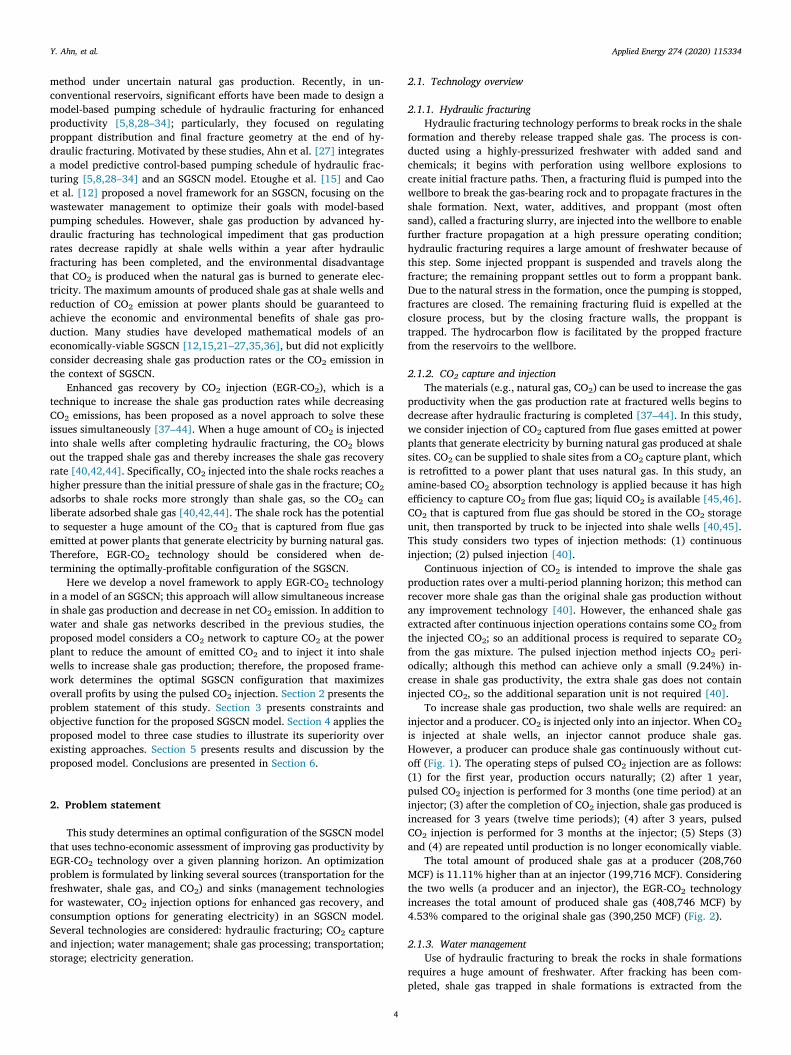
To increase shale gas production, two shale wells are required: aninjector and a producer. CO2 is injected only into an injector. When CO2is injected at shale wells, an injector cannot produce shale gas.However, a producer can produce shale gas continuously without cut-off (Fig. 1). The operating steps of pulsed CO2 injection are as follows:(1) for the first year, production occurs naturally; (2) after 1 year,pulsed CO2 injection is performed for 3 months (one time period) at aninjector; (3) after the completion of CO2 injection, shale gas produced isincreased for 3 years (twelve time periods); (4) after 3 years, pulsedCO2 injection is performed for 3 months at the injector; (5) Steps (3)and (4) are repeated until production is no longer economically viable.

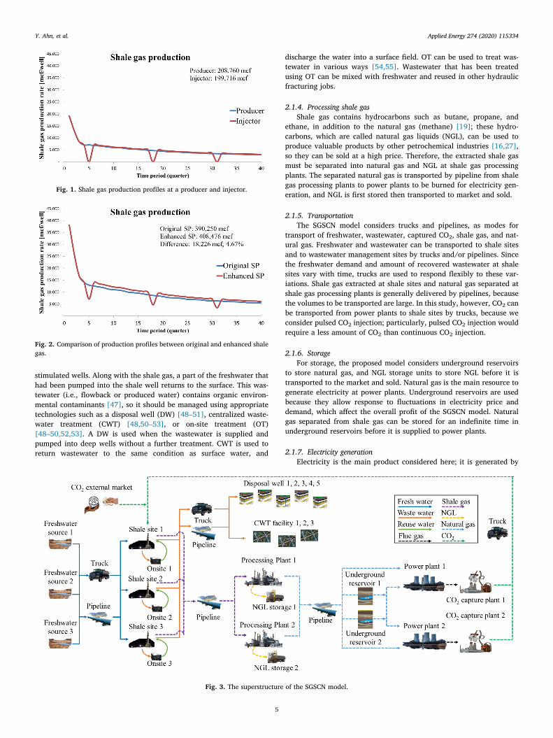
The total amount of produced shale gas at a producer (208,760MCF) is 11.11% higher than at an injector (199,716 MCF). Consideringthe two wells (a producer and an injector), the EGR-CO2 technologyincreases the total amount of produced shale gas (408,746 MCF) by4.53% compared to the original shale gas (390,250 MCF) (Fig. 2).

2.1.3. Water managementUse of hydraulic fracturing to break the rocks in shale formations

requires a huge amount of freshwater. After fracking has been com-pleted, shale gas trapped in shale formations is extracted from the

Y. Ahn, et al. Applied Energy 274 (2020) 115334

4

stimulated wells. Along with the shale gas, a part of the freshwater thathad been pumped into the shale well returns to the surface. This was-tewater (i.e., flowback or produced water) contains organic environ-mental contaminants [47], so it should be managed using appropriatetechnologies such as a disposal well (DW) [48–51], centralized waste-water treatment (CWT) [48,50–53], or on-site treatment (OT)[48–50,52,53]. A DW is used when the wastewater is supplied andpumped into deep wells without a further treatment. CWT is used toreturn wastewater to the same condition as surface water, and

discharge the water into a surface field. OT can be used to treat was-tewater in various ways [54,55]. Wastewater that has been treatedusing OT can be mixed with freshwater and reused in other hydraulicfracturing jobs.

2.1.4. Processing shale gasShale gas contains hydrocarbons such as butane, propane, and

ethane, in addition to the natural gas (methane) [19]; these hydro-carbons, which are called natural gas liquids (NGL), can be used toproduce valuable products by other petrochemical industries [16,27],so they can be sold at a high price. Therefore, the extracted shale gasmust be separated into natural gas and NGL at shale gas processingplants. The separated natural gas is transported by pipeline from shalegas processing plants to power plants to be burned for electricity gen-eration, and NGL is first stored then transported to market and sold.

2.1.5. TransportationThe SGSCN model considers trucks and pipelines, as modes for

transport of freshwater, wastewater, captured CO2, shale gas, and nat-ural gas. Freshwater and wastewater can be transported to shale sitesand to wastewater management sites by trucks and/or pipelines. Sincethe freshwater demand and amount of recovered wastewater at shalesites vary with time, trucks are used to respond flexibly to these var-iations. Shale gas extracted at shale sites and natural gas separated atshale gas processing plants is generally delivered by pipelines, becausethe volumes to be transported are large. In this study, however, CO2 canbe transported from power plants to shale sites by trucks, because weconsider pulsed CO2 injection; particularly, pulsed CO2 injection wouldrequire a less amount of CO2 than continuous CO2 injection.

2.1.6. StorageFor storage, the proposed model considers underground reservoirs

to store natural gas, and NGL storage units to store NGL before it istransported to the market and sold. Natural gas is the main resource togenerate electricity at power plants. Underground reservoirs are usedbecause they allow response to fluctuations in electricity price anddemand, which affect the overall profit of the SGSCN model. Naturalgas separated from shale gas can be stored for an indefinite time inunderground reservoirs before it is supplied to power plants.

2.1.7. Electricity generationElectricity is the main product considered here; it is generated by

Fig. 1. Shale gas production profiles at a producer and injector.

Fig. 2. Comparison of production profiles between original and enhanced shalegas.

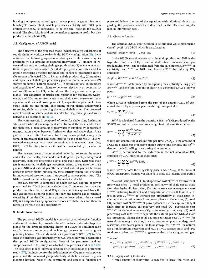
Fig. 3. The superstructure of the SGSCN model.

Y. Ahn, et al. Applied Energy 274 (2020) 115334

5

burning the separated natural gas at power plants. A gas-turbine com-bined-cycle power plant, which generates electricity with 50% gen-eration efficiency, is considered to be the sink node in the SGSCNmodel. The electricity is sold on the market to generate profit, but alsoproduces atmospheric CO2.

2.2. Configuration of SGSCN model

The objective of the proposed model, which use a typical scheme ofsupply chain networks, is to decide the SGSCN configuration (Fig. 3) tooptimize the following operational strategies while maximizing itsprofitability: (1) amount of required freshwater; (2) amount of re-covered wastewater during shale gas production; (3) management op-tions to process wastewater; (4) shale gas production rates and hy-draulic fracturing schedule (original and enhanced production rates);(5) amount of injected CO2 to increase shale productivity; (6) numbersand capacities of shale gas processing plants at potential locations; (7)storage amounts of natural gas and NGL in storage options; (8) numbersand capacities of power plants to generate electricity at potential lo-cations; (9) amount of CO2 captured from the flue gas emitted at powerplants; (10) capacities of trucks and pipelines for freshwater, waste-water, and CO2 among freshwater sites, shale sites, wastewater man-agement facilities, and power plants; (11) capacities of pipeline for twogases (shale gas and natural gas) among power plants, undergroundreservoirs, shale gas processing plants, and shale sites. The proposedmodel consists of source and sinks nodes for CO2, shale gas and waternetworks, as described in Fig. 3.

The water network is composed of nodes for shale sites, freshwatersites, and wastewater management sites. To break the rocks and releasethe shale gas, a huge amount of freshwater is supplied by appropriatetransportation modes between freshwater sites and shale sites. Shalegas is extracted after hydraulic fracturing is completed, along withsome of freshwater that had been injected to the shale wells. This re-covered wastewater with toxic contaminants is managed using DW,CWT, or OT facilities, to which it must be transported by trucks or pi-pelines.

The shale gas network is composed of nodes that represent the sourceand sinks; specifically, these nodes include power plants, undergroundreservoirs, shale gas processing plants, and shale sites. Extracted shalegas is transported to shale gas processing plants to separate the shalegas into NGL and natural gas. The separated natural gas can be trans-ported to power plants immediately for electricity generation, or storedin underground reservoirs and transported to power plants later. TheNGL is stored and later transported to market and sold.

The CO2 network is composed of nodes for CO2 capture at powerplants, and for CO2 injection at shale sites. To increase the shale gasproduction rates, the required CO2 at shale sites is captured from theflue gas emitted at power plants that burn the natural gas to generateelectricity. From the CO2 capture process at power plants, the capturedCO2 is transported using appropriate modes to shale sites and then in-jected to increase the gas productivity.

3. Model formulation

The proposed SGSCN model is composed of an objective functionand several constraints; it was developed from freshwater sites to powerplants for the strategic planning design of SGSCN, to simultaneouslysatisfy demand, resource and technology constraints over a givenplanning horizon. This study modifies a previous SGSCN [27] to con-sider the increased gas productivity by CO2 injection while determiningthe optimal SGSCN configuration. Most of the parameters and as-sumptions used in this study are adopted from previous studies [27,40].The developed model follows a decision structure similar to a previousstudy [27], but incorporates the reduction in net CO2 emission at powerplants, and the increased gas productivity at shale sites over a givenplanning horizon. Most of the constraints and objective function are

presented below; the rest of the equations with additional details re-garding the proposed model are described in the electronic supple-mental information (ESI).

3.1. Objective function

The optimal SGSCN configuration is determined while maximizingOverall profit of SGSCN which is calculated as

=Overeall profit Profit Total cost (1)

In the SGSCN model, electricity is the main product and NGL is thebyproduct, and when CO2 is used at shale sites to increase shale gasproductivity, Profit can be calculated from the sale incomes SIelectricity ofelectricity, and SI NGL of NGL, and benefits SICO2 by reducing CO2emission:

= + +Profit SI SI SIelectricity NGL CO2 (2)

where SIelectricity is determined by multiplying the electricity selling priceprielectricity and the total amount of electricity generated TAGE at powerplants:

=SI pri TAGEelectricity electricity (3)

where TAGE is calculated from the sum of the amount GEm t, of gen-erated electricity at power plant m during time period t:

=TAGE GEm t

m t,(4)

SI NGL is calculated from the quantity PSLSp t, of NGL produced by theSGSCN and sold at shale gas processing plant p during time period t:

=+

SIup PSLS

disr(1 )NGL

p t

tNGL

p tt

,

(5)

where disr denotes the discount rate per time, PSLSp t, is the amount ofNGL sold at shale gas processing plant p during time period t, and upt

NGL

denotes the NGL selling price during time period t.SICO2 is determined by the reduction in the net amount of CO2

emission by CO2 injection at shale sites:

=SI pri CTMICO

m i t

COm i t

2 2, ,

(6)

where priCO2 denotes the CO2 selling price, and CTMIm i t, , is the amountof CO2 transported from power plant m to shale site i during time periodt.

Totalcost is the sum of (1) total operation costTCfresh of freshwater atfreshwater sites; (2) total production cost TCshale of shale gas at shalesites after hydraulic fracturing; (3) total wastewater management costTCwaste including treatment and transportation costs; (4) total CO2 in-jection cost TCCO inject2 to increase gas productivity at shale sites, in-cluding transportation costs from power plants to shale sites; (5) totalCO2 capture cost TCCO capture2 at power plants to use the captured CO2 atshale sites to increase gas recovery; (6) total CO2 purchasing costTCCO pur2 at shale sites to use CO2 to increase gas recovery; (7) totalprocessing cost TCprocessing to separate the natural gas and NGL at shalegas processing plants; (8) total gas transportation cost TCgas trans fornatural gas among shale sites, shale gas processing plants, undergroundreservoirs, and power plants; (9) total storage cost TCstorage for naturalgas at underground reservoirs and NGL at NGL storage units; and (10)total power plant cost TCpower to generate electricity using natural gas:

= + + + + ++ + + +

TotalcostTC TC TC TC TC TC TC TC TC TC

fresh shale CO capture CO inject CO pur

waste processing gas trans storage power

2 2 2

(7)

3.1.1. Supply cost of freshwaterA huge amount of freshwater is required to break the rocks and

Y. Ahn, et al. Applied Energy 274 (2020) 115334

6

release the shale gas at each shale site. The total cost TCfresh of fresh-water is the sum of acquisition cost Cfresh a and the transportation costCfresh t of freshwater from freshwater sites to shale sites:

= +TC C Cfresh fresh a fresh t (8)

where Cfresh a is proportional to the amount of acquired freshwater:

=+

Cuc FWR

disr(1 )fresh a

s i k t

s tacqi

s i k tt

, , , ,

(9)

where FWRs i k t, , , is the supplied amount of freshwater from freshwatersite s to shale site i by transportation mode k during time period t, anducs t

acqi, is the unit acquisition cost of freshwater at freshwater site s during

time period t. Cfresh t includes the capital cost and variable cost of thetransportation modes:

= ++

C ucapc dis XTuvct dis FWR

disr(1 )fresh t

s i k ts i k s i s i k

kfresh

s i s i k tt, ,

1,

1, ,

1 ,1

, , ,

(10)

where diss i,1 denotes the distance from freshwater site s to shale site i,ucapcs i k, ,

1 and uvctkfresh denote, respectively, the unit capital cost and unit

variable cost of transportation mode k from freshwater site s to shalesite i, and XTs i k, ,

1 is a binary variable (i.e., ‘1’ if transportation mode k isselected from freshwater site s to shale site i for freshwater transpor-tation; ‘0’ otherwise).

3.1.2. Production cost of shale gasThe total production cost TCshale of shale gas can be calculated from

the number of hydraulic fracturing jobs and the produced amount ofshale gas at shale sites; its cost includes the several costs for shale gasproduction and hydraulic fracturing jobs considering all shale sites:

=+

++

TCuc NHF

disruc PS

disr(1 ) (1 )shale

i t

i thydraulic

i tt

i t

i tshale production

i tt

, , , ,

(11)

where PSi t, is the shale gas production amount at shale site i during timeperiod t, NHFi t, denotes the number of hydraulic fracturing jobs at shalesite i during time period t, uci t

hydraulic, and uci t

shale production, describe, re-

spectively, the unit costs for shale gas production and hydraulic frac-turing jobs at shale site i during time period t.

3.1.3. Capture and injection cost of CO2CO2 is captured from flue gas to supply the required CO2 to shale

sites; its cost, TCCO capture2 , is the sum of (1) capital costCcc cap of CO2capture plants, (2) operating cost Ccc op of CO2 capture plants, (3)storage costCcc sto of captured CO2, and (4) transportation costCcc tra

from CO2 capture plants to shale sites:

= + + +TC C C C CCO capture cc cap cc op cc sto cc tra2 (12)

where Ccc cap is determined by the capacities of CO2 capture plants:

=C cost Y CEPCIrCEPCI

cc cap

mm mmmCC cap

m mmPCC

CO

CO,2

2 (13)

where Ym mmPCC

, is a binary variable (i.e., ‘1’ if CO2 capture plant m is se-lected with capacity mm for CO2 capture; ‘0’ otherwise), costmm

CC cap is thecapital cost of CO2 capture plant with capacity mm, and CEPCICO2 andrCEPCICO2 denote, respectively, the chemical engineering plant costindex (CEPCI) for CO2 capture plants and their CEPCI of the referenceyear.

Ccc op is calculated from the amount of captured CO2 and operatingparameter of CO2 capture plants:

=C cost capturedCO2cc op

m tmmCC op

m t,(14)

where costmmCC op is the operating cost of CO2 capture plant with capacity

mm, and capturedCO2m t, is the amount of CO2 captured at power plantm during time period t. Before captured CO2 is transported from CO2

capture plants to shale sites, it should be stored in CO2 storage tanks atCO2 capture plants.

CCC sto depends on the amount of stored CO2:

=+

CvcstoredCO

disr2

(1 )CC sto

m t

m tt

,

(15)

where vc denotes the unit storage cost of CO2, and storedCO2m t, is thestorage amount of CO2 at power plant m during time period t. The costof CO2 transport to the shale site is

= ++

C utcc dis XMIuvct dis CTMI

disr(1 )CC tra

m i k tm i kco

m i m i kkCO

m i m i tt, ,

2,

8, ,

72

,8

, ,

(16)

where dism i,8 denotes the distance between power plant m and shale site

i, utccm i kco, ,2 and uvctk

CO2 denote, respectively, the unit capital and variablecost of transportation mode k from power plant m to shale site i,XMIm i k, ,

7 is a binary variable (i.e., ‘1’ if transportation mode k is selectedfor captured CO2 transportation from power plant m to shale site i; ‘0’otherwise), and CTMIm i t, , is the amount of CO2 transported from powerplant m to shale site i during time period t.

The cost of injecting captured CO2 into the shale well is [56,57]:

= + +TC NHF CCR OM m d m( )( )CO inject

i ti t

injection well2,

1 2

(17)

whereCCR is the capital charge rate per year of the total cost,OMinjection

is the operation and maintenance cost rate per year of the total cost forinjection wells,m1 is the cost parameter of well construction, dwell is thewell depth at each shale well, and m2 the cost parameter of injection.

Total CO2 purchasing cost at shale sites TCCO pur2 from externalmarkets is

=TC pri TIACO pur CO CO2 2 2 (18)

where TIACO2 denotes the total amount of injected CO2 at shale sites:

=TIA requiredCO2CO

i ti tpulse2, (19)

where requiredCO2i tpulse, is the total amount of required CO2 at shale site i

during time period t.

3.1.4. Wastewater management costThe total wastewater management cost TCwaste is the sum of (1)

onsite treatment cost Cot; (2) injection cost Cdw injection of disposal well;(3) transportation cost Cdw tra of disposal well; (4) treatment costCCWT tt of CWT facility; and (5) transportation cost CCWT tra of CWTfacility:

= + + + +TC C C C C Cwaste ot dw injection dw tra CWT tt CWT tra (20)

where Cot is the OT treatment cost, and includes the variable cost andcapital cost of the treatment facilities that are selected to reuse thewastewater recovered during shale gas production. In this study, as-suming that the OT facilities operate near the shale sites where hy-draulic fracturing is done, the distance from shale sites to OT facilities isignored:

=+

Cuc WTIO

disr(1 )ot

i o t

oot

i o tt

, ,

(21)

where WTIOi o t, , denotes the treatment amount of wastewater by OTfacility o at shale site i during time period t, and uco

ot is the unit cost atOT facility o to treat wastewater for reuse.

Cdw injection is the injection cost of the wastewater for all disposalwells:

=+

Cuc WTID

disr(1 )dw injection

i d k t

ddw

i d k tt

, , ,

(22)

where WTIDi d k t, , , denotes the transportation amount of wastewater by

Y. Ahn, et al. Applied Energy 274 (2020) 115334

7

mode k between shale site i and disposal well d during time period t,and ucd

dw is the unit disposal cost of disposal well d.Cdw tra is the total transportation cost between shale sites and dis-

posal wells:

= ++

C utcc dis XTuvct dis WTID

disr(1 )dw tra

i d k ti d kdw

i d i d kkwaste

i d i d k tt, , ,

3, ,3 ,

3, , ,

(23)

where disi d,3 denotes the distance between disposal well d and shale site

i, utcci d kdw, , and uvctk

waste denote, respectively, the unit capital and variablecosts of transportation mode k between disposal well d and shale site i,and XTi d k, ,

3 is a binary variable (i.e., ‘1’ if transportation mode k is se-lected from shale site i to disposal well d for wastewater transportation;‘0’ otherwise).

CCWT tt is the CWT facility treatment cost, and includes the oper-ating cost determined by the amount of wastewater transported:

=+

Cuc WTIC

disr(1 )CWT tt

i c k t

cCWT

i c k tt, , ,

(24)

where WTICi c k t, , , denotes the wastewater transported by mode k be-tween CWT facility c and shale site i during time period t, and ucc

CWT isthe unit treatment cost of CWT facility c.

CCWT tra is the total transportation cost for CWT facilities betweenshale sites and CWT facilities:

= ++

C utcc dis XTuvct dis WTIC

disr(1 )CWT tra

i c k ti c kCWT

i c i c kkwaste

i c i c k tt, , ,

2, ,2 ,

2, , ,

(25)

where disi d,2 denotes the distance from shale site i to CWT facility c,

utcci c kCWT, , denotes the unit capital cost of transportation mode k between

CWT facility c and shale site i, and XTi c k, ,2 is a binary variable (i.e., ‘1’ if

transportation mode k is selected between shale site i and CWT facility cfor wastewater transportation; ‘0’ otherwise). The treated wastewater isdischarged as surface water.

3.1.5. Processing cost of shale gasTo separate the shale gas that is extracted after hydraulic fracturing,

a shale gas processing plant is necessary; its total cost TCprocessing isdetermined by considering (1) construction costC ,pro construction (2) op-erating cost C ,pro operating and (3) transportation cost C ,pro transportation ofshale gas processing plants:

= + +TC C C Cprocessing pro construction pro operating pro transportation (26)

Cpro construction is calculated from the capacities of shale gas proces-sing plants, given by:

=C capc Y CEPCIrCEPCI

pro construction

pr pprpro

pr pPC

pro

pro,(27)

where Ypr pPC

, is a binary variable (i.e., ‘1’ if shale gas processing plant p isselected with capacity pr for separation of shale gas; ‘0’ otherwise),capcpr

pro is the capital cost of shale gas processing plants with capacity pr,CEPCI prois the CEPCI for shale gas processing plants, and rCEPCI pro istheir CEPCI for the reference year.

Cpro opeating is the operating cost of shale gas processing plants:

=+

Cuc STIP

disr(1 )pro operating

i p t

proi p t

t, ,

(28)

where STIPi p t, , is the transportation amount of shale gas between shalesite i and shale gas processing plant p during time period t, and uc pro isthe unit processing cost of shale gas at each processing plant.

Cpro transportation is the shale gas transportation cost from shale sites toshale gas processing plants, and includes the capital cost and operatingcost for pipelines:

= +

+

C

capc Y CEPCIrCEPCI

uvct dis STIPdisr(1 )

pro transportation

pi i ppipipe

pi i ppipe TCP

pipe

pipe

i p t

pi si p i p t

t

, ,

,4

, ,

(29)

where CEPCI pipe is the CEPCI for pipelines and rCEPCI pipe is that of thereference year, Ypi i p

pipe TCP, , is a binary variable (i.e., ‘1’ if pipeline capacity

pi is selected for the transportation of natural gas between shale site iand shale gas processing plant p; ‘0’ otherwise), disi p,

4 is the distancefrom shale site i to shale gas processing plant p, capcpi

pipe is the capitalcost of the pipeline with capacity pi, and uvct pi s is the unit variable costof pipeline transportation for shale gas from shale sites to shale gasprocessing plants.

3.1.6. Transportation cost of separated natural gasTo generate electricity, which is the main product in this study,

natural gas separated from shale gas extracted at shale sites must betransported to power plants; this process entails three costs: (1) CNG pm

between shale gas processing plants and power plants; (2) CNG pu be-tween shale gas processing plants and underground reservoirs; and (3)CNG um between underground reservoirs and power plants. The totaltransportation cost considering these three options is calculated as:

= + +TC C C Cgas trans NG pm NG pu NG um (30)

= +

+

C

capc Y dis CEPCIrCEPCI

uvct dis NTPMdisr(1 )

NG pm

pi p mpipipe

pi p mpipe TCPM

p mpipe

pipe

p m t

pi np m p m t

t

, , ,5

,5

, ,

(31)

= +

+

C

capc Y dis CEPCIrCEPCI

uvct dis NTPUdisr(1 )

NG pu

pi p upipipe

pi p upipe TCPU

p upipe

pipe

p m t

pi np u p u t

t

, , ,6

,6

, ,

(32)

= +

+

C

capc Y dis CEPCIrCEPCI

uvct dis NTUMdisr(1 )

NG um

pi u mpipipe

pi u mpipe TCUM

u mpipe

pipe

u m t

pi nu m u m t

t

, , ,7

,7

, ,

(33)

where disp m,5 , disp u,

6 , and disu m,7 denote, respectively, the distances from

shale gas processing plant p to power plant m, from shale gas processingplant p to underground reservoir u, and from underground reservoir uto power plant m. Ypi p m

pipe TCPM, , , Ypi p u

pipe TCPU, , , and Ypi u m

pipe TCUM, , are binary

variables (i.e., respectively, ‘1’ if the pipeline is selected with capacity pifor the natural gas transportation from shale gas processing plant p topower plant m, from shale gas processing plant p to underground re-servoir u, and from underground reservoir u to power plant m; ‘0’otherwise), NTPMp m t, , , NTPUp u t, , , and NTUMu m t, , denote, respectively,the transportation amounts of natural gas from shale gas processingplant p to power plant m, from shale gas processing plant p to under-ground reservoir u, and from underground reservoir u to power plant m,and uvct pi n is the unit variable cost of pipeline for natural gas.

3.1.7. Storage of natural gas and NGLTwo storage options are considered: underground reservoirs for

natural gas and NGL storage units for NGL. The total storage costTCstorage sums the costs of these two options:

Y. Ahn, et al. Applied Energy 274 (2020) 115334

8

=+

++

+

( )TC

uc NTPU uc NTUM

disr

uc SAdisr

(1 )

(1 )

storage

u t

p uunder i

p u t m uunder w

u m t

t

p t

NGLstop tNGL

t

, , , ,

,

(34)

where SAp tNGL, denotes the storage amount of NGL in NGL storage units at

shale gas processing plant p during time period t, ucuunder i and ucu

under w

denote, respectively, the unit costs for the injection and withdrawal ofwastewater at underground reservoir u, and ucNGLsto is the unit NGLstorage cost at NGL storage unit.

3.1.8. Generation cost of electricityThe electricity produced by burning natural gas from the SGSCN is

sold on the market. The total cost TCpower of generating electricity is

=+

+TC ucdisr

NTPM NTUM(1 )

power

m t

mpower

tp

p m tu

u m t, , , ,(35)

where ucmpower is the unit generation cost of electricity at power plant m.

3.2. Constraints

Constraints on freshwater supply, wastewater management, shalegas production, and CO2 capture and injection are described.

3.2.1. Freshwater supplyThe freshwater requirement FWDi t, at shale site i during time period

t is calculated from the number of hydraulic fracturing jobs as:

=FWD acdw NHF i t,i t i i t, , (36)

where acdwi is the freshwater consumption for each hydraulic frac-turing job at shale site i, and NHFi t, is the number of hydraulic frac-turing jobs at shale site i during time period t.

FWDi t, is supplied by the freshwater supply from freshwater sitesand by reusing wastewater treated by OT facilities:

= +FWD FWR rr WTIO i t,i ts k

s i k to

oot

i o t, , , , , ,(37)

where FWRs i k t, , , is the transportation amount of freshwater by mode kbetween freshwater site s and shale site i during time period t,WTIOi o t, ,is the wastewater treatment amount by OT facility o at shale site iduring time period t, and rro

ot is the recovery ratio of treated wastewaterby facility o.

3.2.2. Wastewater generationFor shale gas production, water consumption is important in un-

conventional reservoirs because two types of wastewater are recovered.After hydraulic fracturing has been completed, the amount WPh

i t, ofrecovered wastewater is calculated from the number NHFi t, of hydraulicfracturing jobs at shale site i during time period t, and the recovery ratiorri

h of wastewater at shale site i:

=WP acdw rr NHF i t,hi t i i

hi t, , (38)

Also, the amount WPi ts, of recovered wastewater is calculated from

the ratio that is recovered from the total production amount of shalegas:

=WP ccsw PS i t,si t i i t, , (39)

where PSi t, is the shale gas production amount at shale site i during timeperiod t, and ccswi is the correlation coefficient between the amounts ofproduced shale gas and recovered wastewater at shale site i. To processtwo types of wastewater recovered after hydraulic fracturing has beencompleted, three wastewater management technologies are applied:

+= + +

WP WPWTIC WTID WTIO i t,

hi t

si t

c ki c k t

d ki d k t

o ki o t

, ,

, , , , , , , ,

(40)

where WTIDi d k t, , , and WTICi c k t, , , are, respectively, the transportationamount of wastewater by mode k between shale site i and CWT facilityc, and between shale site i and disposal well d during time period t.

3.2.3. Shale gas productionAfter hydraulic fracturing has been completed, the amount of pro-

duced shale gas at each shale site is given by:

=NHF pr PS i t,tp

i t tpSP

tpshale

i t, , ,(41)

where prtpshale is the shale gas production rate at shale sites during time

period tp, and NHFi t tpSP, , is the number of hydraulic fracturing jobs at

shale site i between time periods t and tp. Details of other constraintsand parameters used in SGSCN are presented in the ESI.

3.2.4. CO2 capture and injectionIn the case of CO2 injection design for SGSCN model, the amount of

shale gas produced at shale sites is equal to the increased amount ofshale gas production at shale sites:

= =PS total i t tp,i t i tpSP enhanced

, , (42)

where PSi t, is the shale gas production amount at shale site i during timeperiod t, and totali tpSP enhanced

, is the increased shale gas productionamount at shale site i during time period tp. When natural gas is burnedto produce electricity at power plants, CO2 is emitted; the amount is:

=powerCO emp GE m t2 ,m t m t m t, , , (43)

where powerCO2m t, denotes the amounts of CO2 emitted at power plantm during time period t, and empm t, is the emission factor for the elec-tricity generation at power plant m during time period t. The amount ofcaptured CO2 cannot exceed the total amount of emitted CO2 at powerplants:

capturedCO powerCO m t2 2 ,m t m t, , (44)

where capturedCO2m t, is the total amount of CO2 captured at powerplant m during time period t. Captured CO2 is held in a storage unit forCO2, then transported to shale sites. The total amount of CO2 stored atpower plant m during time period t is determined by the captured CO2,stored CO2, and transported CO2:

= +storedCO capturedCO storedCO CTMI

m t

2 2 2

,

m t m t m ti

m i t, , , 1 , ,

(45)

where storedCO2m t, is the total amount of CO2 stored at power plant mduring time period t. Finally, the total amount of CO2 required for thepulsed injection is:

=requiredCO CTMI i t2 ,i tpulse

mm i t, , ,

(46)

where requiredCO2i tpulse, is the total CO2 requirement at shale site i during

time period t.

4. Case study

To demonstrate the proposed model for the shale gas productionconsidering enhanced gas productivity, three case studies where theMarcellus shale play is considered were adopted from [16,27]. Thedesign parameters (Table 1) for SGSCN model are taken from the pre-vious studies, and presented in Table1.

Three cases (Fig. 4) are considered in this study as follows: Case 1(SGSCN design with no CO2 injection); Case 2 (SGSCN design with EGR-

Y. Ahn, et al. Applied Energy 274 (2020) 115334

9

CO2 from external markets); Case 3 (SGSCN design with EGR-CO2 fromCO2 capture plants).

To compare the optimal configurations among the three cases, weused ten assumptions:

(1) Shale gas, which has a constant composition, is extracted when thehydraulic fracturing is completed.

(2) Produced shale gas is an ideal gas mixture.(3) Hydraulic fracturing is completed within three months (one time

period)(4) One time period denotes three months, and the total production

period is ten years (forty time periods).(5) Shale gas production rate decreases with time in each well (Table

S1, Figs. S1 and S2).(6) Wastewater with a constant composition is recovered during shale

gas production.(7) CO2 is captured from flue gases for use in pulsed CO2 injection at

shale sites.(8) The capacities of shale gas processing plants for the separation of

shale gas and pipelines for material transportation must be de-termined considering presented data (Table S2).

(9) NGL and electricity generated in power plants are sold.(10) The capacities of CO2 capture plants must be determined con-

sidering presented data (Table S3).Remark 1. In this case study, we have considered a Marcellus shaleplay to determine the optimal configuration of SGSCN considering theenhanced gas recovery by CO2 injection. We have used the dataobtained from a previous study to evaluate the economic feasibility ofthe proposed approach. There is the Brugge benchmarking case byPeters et al. (2010) [66], which is a publicly available dataset of afaulted reservoir with 20 producers and 10 injectors. However, to ourbest knowledge, no research has been performed to determine theoptimal configuration of SGSCN while considering multiple CO2-injection and gas-production wells to increase the shale gasproduction rate. Furthermore, the optimization approach proposed inthis study can be directly applicable to large-scale case studies providedthat necessary optimization models and model parameters areavailable.

5. Results and discussion

This section explains how to determine the optimal configuration ofSGSCN by considering the effect of EGR-CO2 technology to increase theshale gas production rates and decrease the net amount of CO2 emis-sion. The proposed SGSCN model was solved using GAMS 24.3.1(CPLEX 12.6) with Intel® Core™ i5-7200 CPU @2.50 GHz and 16 GBRAM. The proposed problems include 1,166 discrete variables, 46,238continuous variables, and 47,785 constraints.

5.1. Optimal costs

After conducting three case studies, the overall profit of the pro-posed model (Fig. 5) over the 10-year operation was calculated con-sidering the three profits (i.e., incomes by selling NGL and electricity,and benefit by reducing CO2 emission) and ten costs (i.e., gas produc-tion cost, gas transportation cost, gas processing cost, storage cost forshale gas and NGL, power plant cost, wastewater management cost,freshwater transportation cost, CO2 capture cost, CO2 injection cost,and CO2 purchasing cost).

Case 1 and Case 2. The overall profit of Case 2 (US$240 × 106), whichutilized the EGR-CO2 technology for improving gas productivity bypulsed injection using CO2 obtained from the external market, was2.56% higher than that of Case 1 (US$234 × 106), which consideredthe original shale gas production rates without any technology toincrease shale gas productivity. In Case 1 and Case 2, the profitsobtained by income from selling electricity (Case 1: US$415 × 106;Case 2: US$433 × 106) on the external market at US$ 0.1215 per kW∙h[67] dominate the other costs. Sale of NGL separated from shale gas(Case 1: US$28 × 106; Case 2: US$29 × 106) is another major profit inthe optimal costs in both cases. The total costs expect for profit fromelectricity and NGL were Case 1: US$199 × 106; Case 2: US$220 × 106. Specifically, in these cases, the costs of the shale gasprocessing (Case 1: US$158 × 106; Case 2: US$159× 106) included theconstruction costs as well as the operating costs, and were thereforehigher than the other costs. The power plant costs to generateelectricity are the next highest costs (Case 1: US$21 × 106; Case 2:US$22 × 106); they include the costs to transport the natural gas topower plants for electricity generation.

Case 3. The overall profit of Case 3 (US$216 × 106), which utilized theEGR-CO2 technology to increase gas productivity by pulsed injectionusing CO2 obtained from CO2 capture plant, was 7.69% and 10.00%lower than those of Case 1 and Case 2, respectively. The reason is thatthe construction cost of the CO2-capture plant is higher than the CO2benefit obtained by reducing net CO2 emission by CO2 injection at shalesites (CO2 purchasing cost and CO2 benefit are calculated using thesame price; i.e., US$2 per MCF [57]), so in Case 3, the total cost of CO2capture plants including CO2 transportation is US$43 × 106. Theseresults were observed in the optimal configurations of the SGSCN modelcomputed for all three cases.

Table 1Design parameters for SGSCN model.

Papameter Quantity Reference

Freshwater sites 3 [23]Shale sites 3 [58]Maximum number of hydraulic fracturing jobs 6 [5]Disposal wells 5 [59]CWT facilities 3 [60,61]OT technologies MSF, MED, and RO [60,61]Shale gas processing plants 2 [62]Power plants 2 [63,64]Underground reservoirs 2 [65]CO2 capture plants 2 [40,45]Transportation modes Truck and pipeline [16]Total planning horizon 10 years [22]

Fig. 4. Simplified SGSCN diagrams for the three case studies.

Y. Ahn, et al. Applied Energy 274 (2020) 115334

10

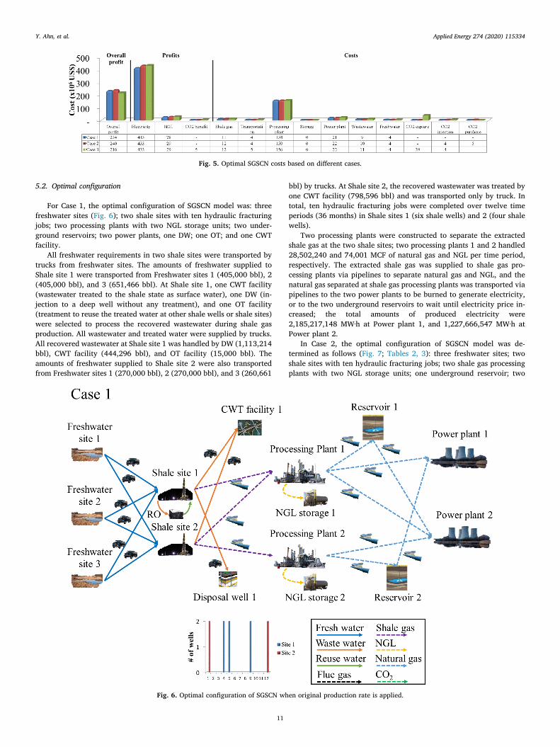
5.2. Optimal configuration

For Case 1, the optimal configuration of SGSCN model was: threefreshwater sites (Fig. 6); two shale sites with ten hydraulic fracturingjobs; two processing plants with two NGL storage units; two under-ground reservoirs; two power plants, one DW; one OT; and one CWTfacility.

All freshwater requirements in two shale sites were transported bytrucks from freshwater sites. The amounts of freshwater supplied toShale site 1 were transported from Freshwater sites 1 (405,000 bbl), 2(405,000 bbl), and 3 (651,466 bbl). At Shale site 1, one CWT facility(wastewater treated to the shale state as surface water), one DW (in-jection to a deep well without any treatment), and one OT facility(treatment to reuse the treated water at other shale wells or shale sites)were selected to process the recovered wastewater during shale gasproduction. All wastewater and treated water were supplied by trucks.All recovered wastewater at Shale site 1 was handled by DW (1,113,214bbl), CWT facility (444,296 bbl), and OT facility (15,000 bbl). Theamounts of freshwater supplied to Shale site 2 were also transportedfrom Freshwater sites 1 (270,000 bbl), 2 (270,000 bbl), and 3 (260,661

bbl) by trucks. At Shale site 2, the recovered wastewater was treated byone CWT facility (798,596 bbl) and was transported only by truck. Intotal, ten hydraulic fracturing jobs were completed over twelve timeperiods (36 months) in Shale sites 1 (six shale wells) and 2 (four shalewells).

Two processing plants were constructed to separate the extractedshale gas at the two shale sites; two processing plants 1 and 2 handled28,502,240 and 74,001 MCF of natural gas and NGL per time period,respectively. The extracted shale gas was supplied to shale gas pro-cessing plants via pipelines to separate natural gas and NGL, and thenatural gas separated at shale gas processing plants was transported viapipelines to the two power plants to be burned to generate electricity,or to the two underground reservoirs to wait until electricity price in-creased; the total amounts of produced electricity were2,185,217,148 MW∙h at Power plant 1, and 1,227,666,547 MW∙h atPower plant 2.

In Case 2, the optimal configuration of SGSCN model was de-termined as follows (Fig. 7; Tables 2, 3): three freshwater sites; twoshale sites with ten hydraulic fracturing jobs; two shale gas processingplants with two NGL storage units; one underground reservoir; two

Fig. 5. Optimal SGSCN costs based on different cases.

Fig. 6. Optimal configuration of SGSCN when original production rate is applied.

Y. Ahn, et al. Applied Energy 274 (2020) 115334

11

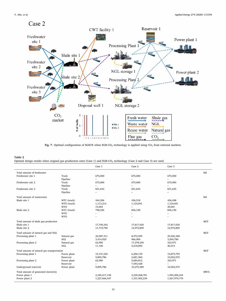
Fig. 7. Optimal configuration of SGSCN when EGR-CO2 technology is applied using CO2 from external markets.

Table 2Optimal design results when original gas production rates (Case 1) and EGR-CO2 technology (Case 2 and Case 3) are used.

Case 1 Case 2 Case 3

Total amount of freshwater bblFreshwater site 1 Truck 675,000 675,000 675,000

Pipeline – – –Freshwater site 2 Truck 675,000 675,000 675,000

Pipeline – – –Freshwater site 3 Truck 651,644 651,654 651,645

Pipeline – – –

Total amount of wastewater bblShale site 1 WTC (truck) 444,296 436,518 436,498

WTD (truck) 1,113,214 1,124,841 1,124,841WTO 15,003 – 20,001

Shale site 2 WTC (truck) 798,596 836,190 836,190WTD – – –WTO – – –

Total amount of shale gas production MCFShale site 1 17,740,342 17,817,020 17,817,020Shale site 2 11,719,700 12,972,809 12,972,809

Total amount of natural gas and NGL MCFProcessing plant 1 Natural gas 25,087,311 8,972,099 25,926,368

NGL 3,414,929 966,900 3,569,780Processing plant 2 Natural gas 62,900 17,278,240 323,971

NGL 11,100 2,618,895 46,014

Total amount of natural gas transportation MCFProcessing plant 1 Power plant 15,191,525 6,290,139 15,873,793

Reservoir 9,895,786 2,681,960 10,052,575Processing plant 2 Power plant 62,900 9,684,812 323,971

Reservoir – 7,593,428 –Underground reservoir Power plant 9,895,786 10,275,389 10,052,575

Total amount of generated electricity MW∙hPower plant 1 2,185,217,148 2,230,268,781 1,994,200,244Power plant 2 1,227,666,547 1,331,902,234 1,567,970,770

Y. Ahn, et al. Applied Energy 274 (2020) 115334

12

power plants; one CWT facility; and one DW.Ten hydraulic fracturing jobs were completed over twelve time

periods in Shale sites 1 (six shale wells) and 2 (four shale wells). OneDW and CWT facility were placed at two shale sites to treat the was-tewater recovered at shale sites. CO2 for injection was purchased fromexternal markets; their amounts were 1,350,721 MCF at Shale site 1and 1,026,663 MCF at Shale site 2.

In Case 3, the optimal configuration of SGSCN model was de-termined as follows (Fig. 8; Tables 2, 3): three freshwater sites; twoshale sites with ten hydraulic fracturing jobs; two shale gas processingplants with two NGL storage units; one OT facility; one undergroundreservoir; one CO2 capture plant; two power plants; one DW; and oneCWT facility.

Ten hydraulic fracturing jobs were completed over twelve timeperiods in Shale sites 1 (six shale wells) and 2 (four shale wells), as in

Case 1 and Case 2. In Case 3, MED technology was selected to treat therecovered wastewater, and then the treated wastewater was reused inother shale sites or shale wells. In this case, CO2 was captured from fluegas emitted at power plants as they burned natural gas to generateelectricity, then transported by trucks and injected at the two shalesites. Transport of the required CO2 to the two shale sites required twotrucks; the amounts from CO2 capture plant 1 were 1,350,721 MCF toShale site 1, and 1,206,663 MCF to Shale site 2.

5.3. Optimal production of shale gas

The task of break the rocks at shale sites required ten hydraulicfracturing jobs in all three cases; but the total amount of shale gasproduced was different. Case 1 produced 29.5 × 106 MCF, whereasCase 2 and Case 3 both produced 30.8 × 106 MCF (Fig. 9), i.e., 4.41%more than by Case 1.

Optimal SGSCN configurations that maximize the overall profit withoptimal schedules of hydraulic fracturing operations were determinedfor the three cases (Figs. 6–8). After fracking had been completed, mostof the shale gas was produced within a year, and then the rates de-creased rapidly over time. Synchronizing the presentation to have hy-draulic fracturing jobs completed at the same time yielded the trends inthe production profile of shale gas (Fig. 9). After the 12th time period,the trends in the gas production showed only decreases, because hy-draulic fracturing operation should be completed within 36 months(twelve time periods; 3 years); otherwise, the gas production profilecould increase without the constraint.

5.4. Optimal schedule of CO2 injection

In both Case 2 and Case 3, pulsed injection of CO2 is used to increasethe shale gas production rates at all shale sites. To maximize the overallprofit of the SGSCN, the optimal schedules of pulsed CO2 injection were

Table 3Optimal design results when EGR-CO2 technology is used.

Case 1 Case 2 Case 3

Total amount of emitted CO2 MCFPower plant 1 11,575,858 11,814,512 10,563,975Power plant 2 9,078,973 9,849,829 11,595,628

Total amount of captured CO2 – – 2,378,955 MCFPower plant 1 – – 2,378,955Power plant 2 – – –

Total amount of stored CO2 – – MCFPower plant 1 – – 1,863,141Power plant 2 – –

Total amount of injected CO2 – MCFExternal market Shale site 1 – 1,350,721

Shale site 2 – 1,026,663Power plant 1 Shale site 1 – – 1,350,721

Shale site 2 – – 1,206,663

Fig. 8. Optimal configuration of SGSCN when EGR-CO2 technology is applied using CO2 from CO2 capture plants.

Y. Ahn, et al. Applied Energy 274 (2020) 115334

13

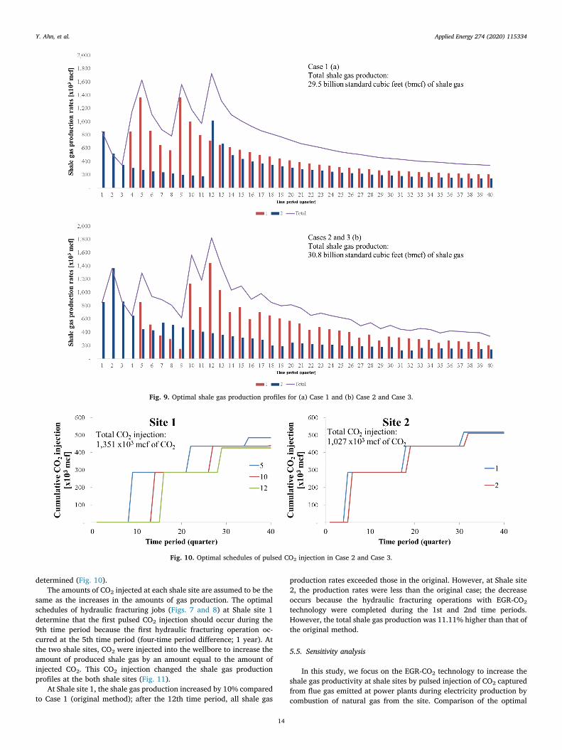
determined (Fig. 10).The amounts of CO2 injected at each shale site are assumed to be the

same as the increases in the amounts of gas production. The optimalschedules of hydraulic fracturing jobs (Figs. 7 and 8) at Shale site 1determine that the first pulsed CO2 injection should occur during the9th time period because the first hydraulic fracturing operation oc-curred at the 5th time period (four-time period difference; 1 year). Atthe two shale sites, CO2 were injected into the wellbore to increase theamount of produced shale gas by an amount equal to the amount ofinjected CO2. This CO2 injection changed the shale gas productionprofiles at the both shale sites (Fig. 11).

At Shale site 1, the shale gas production increased by 10% comparedto Case 1 (original method); after the 12th time period, all shale gas

production rates exceeded those in the original. However, at Shale site2, the production rates were less than the original case; the decreaseoccurs because the hydraulic fracturing operations with EGR-CO2technology were completed during the 1st and 2nd time periods.However, the total shale gas production was 11.11% higher than that ofthe original method.

5.5. Sensitivity analysis

In this study, we focus on the EGR-CO2 technology to increase theshale gas productivity at shale sites by pulsed injection of CO2 capturedfrom flue gas emitted at power plants during electricity production bycombustion of natural gas from the site. Comparison of the optimal

Fig. 9. Optimal shale gas production profiles for (a) Case 1 and (b) Case 2 and Case 3.

Fig. 10. Optimal schedules of pulsed CO2 injection in Case 2 and Case 3.

Y. Ahn, et al. Applied Energy 274 (2020) 115334

14

costs (Fig. 5) confirms that the overall profit of SGSCN (Case 3) waslower than those in Case 1 and 2. An increase in the benefit obtainedfrom reducing CO2 emission by CO2 injection may increase the eco-nomic feasibility of using recaptured CO2 gas (Case 3) compared to Case1. To check the economics of CO2 capture plant in the SGSCN model,the proposed system evaluated the effects of CO2 prices between US$2and US$6 per MCF (Table 4).

From the sensitivity analysis results for CO2 price, the overall profitof the SGSCN model in Case 3 exceeds that of Case 2 when the CO2 priceexceeds US$5 per MCF. This sensitivity analysis predicts that the EGR-CO2 technology using CO2 obtained by CO2 capture plant can be used toincrease the shale gas production rates and decrease the net CO2emission that occurs by burning it. For EGR-CO2 that uses CO2 fromCO2 capture plants to be profitable, the CO2 price must be greater thanUS$5 per MCF.

Remark 2. The proposed approach can be further extended to a multi-period optimization model by taking into account actual locations of avariety of wastewater treatment and shale gas processing facilities aswell as water sources and disposal wells. Specifically, these real fielddata can be integrated with our optimization model in the form ofdifferences in model parameters and cost coefficients, which cansignificantly affect the optimal configuration of SGSCN. However, oneof the key challenges is that to our best knowledge, a comprehensivereview of these real field data has never been reported in the literaturebecause either they are not publicly available or there data aredistributed over multiple database sources.

6. Conclusions

In this study, we evaluated the effectiveness of enhanced gas re-covery by carbon dioxide (CO2) injection’ (EGR-CO2) technology, whichinjects CO2 that is emitted when the shale gas is burned to produceelectricity to simultaneously increase shale gas production and decreasenet CO2 emissions. We used a mixed-integer linear programming pro-blem, which determined the optimal configuration of supply chainnetwork for shale gas production (SGSCN) that maximizes the overallprofit by pulsed CO2 injection; the amounts of injected CO2, the

increase in shale gas production rate, and the net CO2 reduction byinjecting it into fractured wells were considered. The overall profit ofCase 2, which uses EGR-CO2 technology but buys CO2 externally, was2.56% higher than that of Case 1, which considers only the normalproduction rates of shale gas in an SGSCN model. However, Case 3,which uses EGR-CO2 using CO2 from CO2 capture plants, achievedlower overall profit by 7.69% compared to Case 1, and by 10.00%compared to Case 2, because the total additional cost of building andoperating CO2-capture plants was higher than the total benefit of CO2injection at shale sites. For Case 3 to achieve profit that exceeds Case 2,the market price of CO2 must be greater than US$5 per MCF (0.18 US$per m3). This study indicates that the total profit of shale gas extractioncan be improved by applying the pulsed CO2 injection, because it in-creases shale gas productivity.

CRediT authorship contribution statement

Yuchan Ahn: Conceptualization, Methodology, Validation, Formalanalysis, Investigation, Writing - original draft, Writing - review &editing, Visualization. Junghwan Kim: Writing - review & editing,Supervision, Project administration, Funding acquisition. Joseph Sang-Il Kwon: Conceptualization, Methodology, Formal analysis, Resources,Writing - review & editing, Supervision, Project administration,Funding acquisition.

Declaration of Competing Interest

The authors declare that they have no known competing financialinterests or personal relationships that could have appeared to influ-ence the work reported in this paper.

Acknowledgment

The authors gratefully acknowledge financial support from theNational Science Foundation (CBET-1804407), U.S. Department ofEnergy (DE-EE000788-10-8, DE-EE000788-9.3), the Korea Institute ofIndustrial Technology (kitech IR-19-0021, kitech JH-20-0005).

Appendix A. Supplementary material

Supplementary data to this article can be found online at https://doi.org/10.1016/j.apenergy.2020.115334.

References

[1] Middleton RS, Gupta R, Hyman JD, Viswanathan HS. The shale gas revolution:Barriers, sustainability, and emerging opportunities. Appl Energy 2017;199:88–95.

[2] Weijermars R. Shale gas technology innovation rate impact on economic Base Case-Scenario model benchmarks. Appl Energy 2015;139:398–407.

[3] Feijoo F, Iyer GC, Avraam C, Siddiqui SA, Clarke LE, Sankaranarayanan S, et al. The

Fig. 11. Comparison of the shale gas production profiles based on the original gas production and enhanced gas production in Case 2 and Case 3.

Table 4Sensitivity analysis results among the variation of CO2 price for the overallprofit of the SGSCN model in Case 2 and Case 3.

US$/MCF of CO2 Case 2 (×US$ 106) Case 3 (×US$ 106)

2 240 2163 239 2174 238 2205 233 2326 230 234

Y. Ahn, et al. Applied Energy 274 (2020) 115334

15

future of natural gas infrastructure development in the United states. Appl Energy2018;228:149–66.

[4] Yuan J, Luo D, Feng L. A review of the technical and economic evaluation techni-ques for shale gas development. Appl Energy 2015;148:49–65.

[5] Siddhamshetty P, Kwon J-I, Liu S, Valkó PP. Feedback control of proppant bankheights during hydraulic fracturing for enhanced productivity in shale formations.AIChE J. 2018;64(5):1638–50.

[6] Wang K, Li H, Wang J, Jiang B, Bu C, Zhang Q, et al. Predicting production andestimated ultimate recoveries for shale gas wells: A new methodology approach.Appl Energy 2017;206:1416–31.

[7] Loucks RG, Reed RM, Ruppel SC, Jarvie DM. Morphology, genesis, and distributionof nanometer-scale pores in siliceous mudstones of the Mississippian Barnett Shale.J Sediment Res 2009;79:848–61.

[8] Siddhamshetty P, Wu K, Kwon J-S-I. Modeling and control of proppant distributionof multistage hydraulic fracturing in horizontal shale wells. Ind Eng Chem Res2019;58:3159–69.

[9] Middleton RS, Carey JW, Currier RP, Hyman JD, Kang Q, Karra S, et al. Shale gasand non-aqueous fracturing fluids: Opportunities and challenges for supercriticalCO2. Appl Energy 2015;147:500–9.

[10] Chang Y, Huang R, Ries RJ, Masanet E. Shale-to-well energy use and air pollutantemissions of shale gas production in China. Appl Energy 2014;125:147–57.

[11] Kang D, Lim HS, Lee M, Lee JW. Syngas production on a Ni-enhanced Fe2O3/Al2O3oxygen carrier via chemical looping partial oxidation with dry reforming of me-thane. Appl Energy 2018;211:174–86.

[12] Cao K, Siddhamshetty P, Ahn Y, Mukherjee R, Kwon JS-I. Economic model-basedcontroller design framework for hydraulic fracturing to optimize shale gas pro-duction and water usage. Ind Eng Chem Res 2019.

[13] DeNooyer TA, Peschel JM, Zhang Z, Stillwell AS. Integrating water resources andpower generation: the energy–water nexus in Illinois. Appl Energy2016;162:363–71.

[14] Huang B, Liu C, Fu J, Guan H. Hydraulic fracturing after water pressure controlblasting for increased fracturing. Int J Rock Mech Min Sci 2011;48:976–83.

[15] Etoughe P, Siddhamshetty P, Cao K, Mukherjee R, Kwon J-S-I. Incorporation ofsustainability in process control of hydraulic fracturing in unconventional re-servoirs. Chem Eng Res Des 2018;139:62–76.

[16] Gao J, You F. Shale gas supply chain design and operations toward better economicand life cycle environmental performance: MINLP model and global optimizationalgorithm. ACS Sustainable Chem Eng 2015;3:1282–91.

[17] Jiang M, Griffin WM, Hendrickson C, Jaramillo P, VanBriesen J, Venkatesh A. Lifecycle greenhouse gas emissions of Marcellus shale gas. Environ Res Lett2011;6:034014.

[18] Hultman N, Rebois D, Scholten M, Ramig C. The greenhouse impact of unconven-tional gas for electricity generation. Environ Res Lett 2011;6:044008.

[19] Administration UEI. Natural gas processing plants in the United States: 2010Update; 2011.

[20] Beamon BM. Supply chain design and analysis: Models and methods. Int J ProdEcon 1998;55:281–94.

[21] Gao J, You F. Optimal design and operations of supply chain networks for watermanagement in shale gas production: MILFP model and algorithms for the water-energy nexus. AIChE J 2015;61:1184–208.

[22] Cafaro DC, Grossmann IE. Strategic planning, design, and development of the shalegas supply chain network. AIChE J 2014;60:2122–42.

[23] Yang L, Grossmann IE, Manno J. Optimization models for shale gas water man-agement. AIChE J 2014;60:3490–501.

[24] Guerra OJ, Calderón AJ, Papageorgiou LG, Siirola JJ, Reklaitis GV. An optimizationframework for the integration of water management and shale gas supply chaindesign. Comput Chem Eng 2016;92:230–55.

[25] Chebeir J, Geraili A, Romagnoli J. Development of shale gas supply chain networkunder market uncertainties. Energies 2017;10:246.

[26] Chen Y, He L, Li J, Zhang S. Multi-criteria design of shale-gas-water supply chainsand production systems towards optimal life cycle economics and greenhouse gasemissions under uncertainty. Comput Chem Eng 2018;109:216–35.

[27] Ahn Y, Siddhamshetty P, Cao K, Han J, Kwon J-S-I. Optimal design of shale gassupply chain network considering MPC-based pumping schedule of hydraulicfracturing in unconventional reservoirs. Chem Eng Res Des 2019;147:412–29.

[28] Siddhamshetty P, Bhandakkar P, Kwon J-S-I. Enhancing total fracture surface areain naturally fractured unconventional reservoirs via model predictive control. JPetrol Sci Eng 2020;184:106525.

[29] Siddhamshetty P, Wu K, Kwon J-S-I. Optimization of simultaneously propagatingmultiple fractures in hydraulic fracturing to achieve uniform growth using data-based model reduction. Chem Eng Res Des 2018;136:675–86.

[30] Narasingam A, Siddhamshetty P, Kwon J-S-I. POD-based EnKF estimation of het-erogeneous reservoir parameters for feedback control of hydraulic fracturing.Comput Aid Chem Eng 2018:733–8.

[31] Narasingam A, Kwon J-S-I. Development of local dynamic mode decompositionwith control: Application to model predictive control of hydraulic fracturing.Comput Chem Eng 2017;106:501–11.

[32] Siddhamshetty P, Yang S, Kwon J-S-I. Modeling of hydraulic fracturing and de-signing of online pumping schedules to achieve uniform proppant concentration inconventional oil reservoirs. Comput Chem Eng 2018;114:306–17.

[33] Gu Q, Hoo KA. Evaluating the performance of a fracturing treatment design. IndEng Chem Res 2014;53:10491–503.

[34] Gu Q, Hoo KA. Model-based closed-loop control of the hydraulic fracturing process.Ind Eng Chem Res 2015;54:1585–94.

[35] Lira-Barragán LF, Ponce-Ortega JM, Guillén-Gosálbez G, El-Halwagi MM. Optimal

water management under uncertainty for shale gas production. Ind Eng Chem Res2016;55:1322–35.

[36] Arredondo-Ramírez K, Ponce-Ortega JM, El-Halwagi MM. Optimal planning andinfrastructure development for shale gas production. Energy Convers Manage2016;119:91–100.

[37] Tang L, Sun S, Mi L, Wang L, Qi H, Yu R, et al. Analysis of enhancement shale gasrecovery by CO2 storage. SPE Argentina exploration and production of unconven-tional resources symposium. Society of Petroleum Engineers; 2016.

[38] Godec M, Koperna G, Petrusak R, Oudinot A. Assessment of factors influencing CO2storage capacity and injectivity in Eastern US Gas Shales. Energy Procedia2013;37:6644–55.

[39] Godec M, Koperna G, Petrusak R, Oudinot A. Enhanced gas recovery and CO2storage in gas shales: a summary review of its status and potential. Energy Procedia2014;63:5849–57.

[40] Li X, Elsworth D. Geomechanics of CO2 enhanced shale gas recovery. J Nat Gas SciEng 2015;26:1607–19.

[41] Fathi E, Akkutlu IY. Multi-component gas transport and adsorption effects duringCO2 injection and enhanced shale gas recovery. Int J Coal Geol 2014;123:52–61.

[42] Godec M, Koperna G, Petrusak R, Oudinot A. Potential for enhanced gas recoveryand CO2 storage in the Marcellus Shale in the Eastern United States. Int J Coal Geol2013;118:95–104.

[43] Godec ML, Jonsson H, Basava-Reddi L. Potential global implications of gas pro-duction from shales and coal for geological CO2 storage. Energy Procedia2013;37:6656–66.

[44] Pei P, Ling K, He J, Liu Z. Shale gas reservoir treatment by a CO2-based technology.J Nat Gas Sci Eng 2015;26:1595–606.

[45] Ahn Y-C, Lee I-B, Lee K-H, Han J-H. Strategic planning design of microalgae bio-mass-to-biodiesel supply chain network: Multi-period deterministic model. ApplEnergy 2015;154:528–42.

[46] Kim J, Johnson TA, Miller JE, Stechel EB, Maravelias CT. Fuel production from CO2 using solar-thermal energy: system level analysis. Energy Environ Sci2012;5:8417–29.

[47] Annevelink M, Meesters J, Hendriks A. Environmental contamination due to shalegas development. Sci Total Environ 2016;550:431–8.

[48] Bartholomew TV, Mauter MS. Multiobjective optimization model for minimizingcost and environmental impact in shale gas water and wastewater management.ACS Sustainable Chem Eng 2016;4:3728–35.

[49] Horner P, Halldorson B, Slutz JA. Shale gas water treatment value chain-a review oftechnologies, including case studies. SPE annual technical conference and exhibi-tion. Society of Petroleum Engineers; 2011.

[50] Slutz JA, Anderson JA, Broderick R, Horner PH. Key shale gas water managementstrategies: An economic assessment. International conference on health, safety andenvironment in oil and gas exploration and production. Society of PetroleumEngineers; 2012.

[51] Wilson JM, VanBriesen JM. Oil and gas produced water management and surfacedrinking water sources in Pennsylvania. Environ Pract 2012;14:288–300.

[52] Lutz BD, Lewis AN, Doyle MW. Generation, transport, and disposal of wastewaterassociated with Marcellus Shale gas development. Water Resour Res2013;49:647–56.

[53] Olmstead SM, Muehlenbachs LA, Shih J-S, Chu Z, Krupnick AJ. Shale gas devel-opment impacts on surface water quality in Pennsylvania. Proc Natl Acad Sci2013;110:4962–7.

[54] Jang E, Jeong S, Chung E. Application of three different water treatment technol-ogies to shale gas produced water. Geosyst Eng 2017;20:104–10.

[55] Van der Bruggen B, Vandecasteele C. Distillation vs. membrane filtration: overviewof process evolutions in seawater desalination. Desalination 2002;143:207–18.

[56] Ogden J. Conceptual design of optimized fossil energy systems with capture andsequestration of carbon dioxide; 2004.

[57] Hasan MF, Boukouvala F, First EL, Floudas CA. Nationwide, regional, and statewideCO2 capture, utilization, and sequestration supply chain network optimization. IndEng Chem Res 2014;53:7489–506.

[58] Ladlee J, Jacquet J. The implications of multi-well pads in the Marcellus. Shale.2011.

[59] Veil JA. Final report water management technologies used by Marcellus shale gasproducers. NETL; 2010.

[60] Al-Nory MT, Brodsky A, Bozkaya B, Graves SC. Desalination supply chain decisionanalysis and optimization. Desalination 2014;347:144–57.

[61] Raluy G, Serra L, Uche J. Life cycle assessment of MSF, MED and RO desalinationtechnologies. Energy 2006;31:2361–72.

[62] He C, You F. Shale gas processing integrated with ethylene production: novelprocess designs, exergy analysis, and techno-economic analysis. Ind Eng Chem Res2014;53:11442–59.

[63] Weber CL, Clavin C. Life cycle carbon footprint of shale gas: Review of evidence andimplications. Environ Sci Technol 2012;46:5688–95.

[64] Cost L. Levelized avoided cost of new generation resources in the annual energyoutlook 2014. US Energy Information Administration; 2014.

[65] Kumar G, Shobana S, Chen W-H, Bach Q-V, Kim S-H, Atabani A, et al. A review ofthermochemical conversion of microalgal biomass for biofuels: chemistry andprocesses. Green Chem 2017;19:44–67.

[66] Peters L, Arts R, Brouwer G, Geel C, Cullick S, Lorentzen RJ, et al. Results of theBrugge benchmark study for flooding optimization and history matching. SPEReservoir Eval Eng 2010;13:391–405.

[67] Administration. USEI. Electric power monthly. https://www.eia.gov/electricity/monthly/epm_table_grapher.php?t=epmt_5_6_a [accessed 2/7/19].

Y. Ahn, et al. Applied Energy 274 (2020) 115334

16