Optimal Control of a BuildingDuring an Earthquake

Kenneth Maples

Prof. Weiqing Gu, Advisor

Prof. Anthony Bright (Engineering), Reader

May, 2006

Department of Mathematics

Copyright c© 2006 Kenneth Maples.

The author grants Harvey Mudd College the nonexclusive right to make this workavailable for noncommercial, educational purposes, provided that this copyrightstatement appears on the reproduced materials and notice is given that the copy-ing is by permission of the author. To disseminate otherwise or to republish re-quires written permission from the author.

Abstract

In this thesis I develop a mathematical model for an apartment buildingduring an earthquake. The movement of the building is restricted to aplane and twisting motions have been assumed negligible. A control sys-tem for the building is developed using optimal control techniques. Fora quadratic objective functional, the existence of an optimal control is de-termined and numerical results are generated that show that the controllersignificantly lowers the chaotic oscillations in the building. The numericalwork was done with the Miser3 package for Matlab. Relaxation of differ-ent constraints are considered, including multiple controls, varying stories,and different objective functionals.

Contents

Abstract iii

Acknowledgments ix

1 Introduction 11.1 Model Derivation . . . . . . . . . . . . . . . . . . . . . . . . . 21.2 Background . . . . . . . . . . . . . . . . . . . . . . . . . . . . 51.3 Paper Organization . . . . . . . . . . . . . . . . . . . . . . . . 6

2 A Mathematical Model 92.1 Equations of Motion . . . . . . . . . . . . . . . . . . . . . . . 92.2 Matrix Equations . . . . . . . . . . . . . . . . . . . . . . . . . 12

3 Optimal Control of the Model 173.1 Quadratic Controls . . . . . . . . . . . . . . . . . . . . . . . . 173.2 Existence of an Optimal Control . . . . . . . . . . . . . . . . . 18

4 Multiple Floors 214.1 Mathematical Development . . . . . . . . . . . . . . . . . . . 22

5 State Constraints 255.1 Analysis . . . . . . . . . . . . . . . . . . . . . . . . . . . . . . 255.2 Numerics . . . . . . . . . . . . . . . . . . . . . . . . . . . . . . 26

6 Numerical Results 276.1 Miser3 . . . . . . . . . . . . . . . . . . . . . . . . . . . . . . . 276.2 Results for Four Stories and One Control . . . . . . . . . . . 346.3 Results for Multiple Stories . . . . . . . . . . . . . . . . . . . 34

vi Contents

7 Discussion and Future Work 377.1 Linear Controls . . . . . . . . . . . . . . . . . . . . . . . . . . 377.2 Continuous Model . . . . . . . . . . . . . . . . . . . . . . . . 387.3 Future Work and Conclusions . . . . . . . . . . . . . . . . . . 39

Bibliography 41

List of Figures

1.1 A four story apartment building . . . . . . . . . . . . . . . . 21.2 Modeling takes natural phenomena and represents them math-

ematically . . . . . . . . . . . . . . . . . . . . . . . . . . . . . 31.3 A particle model for the building . . . . . . . . . . . . . . . . 31.4 A continuous model for the building . . . . . . . . . . . . . . 41.5 The same apartment building separated into lumped masses

for each floor. . . . . . . . . . . . . . . . . . . . . . . . . . . . 5

2.1 The forces between adjacent floors must be determined. . . . 102.2 Linear springs do not match observational data. . . . . . . . 102.3 An example bilinear hysteretic force. . . . . . . . . . . . . . . 112.4 Nobody seems to have explored non-linear damper behavior. 112.5 A tuned mass is attached to the top floor of the building. . . 122.6 A tuned mass is attaached to the building through a spring

and damper. . . . . . . . . . . . . . . . . . . . . . . . . . . . . 12

6.1 The simple model with a Dirac delta input and no control. . 356.2 The simple model with a Dirac delta input and an optimal

control. . . . . . . . . . . . . . . . . . . . . . . . . . . . . . . . 36

Acknowledgments

I would like to thank Professor Gu for her mentoring throughout my un-dergraduate education. Her zeal and energy has motivated me when thepath ahead seemed rough.

Also, I would like to thank my family for the care and love they havegiven me.

Finally, I must thank Claire Connelly for her technical assistance, SuzanneFrantz for her daily help, and my classmates for making math and engi-neering fun every day.

Chapter 1

Introduction

Suppose we are asked to develop a system for minimizing the damagethat a building receives during an earthquake. The first, and most obviousmethod for minimizing earthquake damage is passive systems. Naturally,modern construction techniques allow for buildings to resist all but thestrongest earthquakes without severe damage to the structural integrity.However, the problem that an earthquake provides is not a simple ques-tion that can be answered with vibration dampers are creative constructiontechniques.

When an earthquake hits a building, it causes vibrational energy to en-ter the structure which creates waves that travel up and down the building,shaking the structure from side to side. The energy stored in these waves istransferred into heat by the friction inside the walls and by the resistance ofthe air surrounding the building. However, excessive vibrations can causetears in the wall material which can cause structural failure in the building,triggering the collapse of the building and the deaths of its inhabitants. Pas-sive devices limit the risks of building failure by redirecting the energy ofthese waves into specific points where the resonant frequency of the build-ing is damped and contained; these sections will not cause the structuralfailure of the building when they absorb large amounts of kinetic energy.

However, we as building designers can surpass the effects of passivedesign by applying active control techniques to counteract the earthquake.By storing energy in the building before the earthquake hits, an activemechanism can release energy into the building that will counteract the en-ergy of the earthquake and dampen the movement of the structure. In thisway, we can begin to dissipate the energy of the earthquake at a slow ratebefore the earthquake hits, which allows larger earthquakes to be handled

2 Introduction

Figure 1.1: A four story apartment building

by the building.Correctly applying active control techniques to “cancel” the earthquake

is not an obvious task. Improperly designed controllers could instead worsenthe effects of the earthquake by either amplifying the earthquake signal orby creating whiplash effects, where the two waves cancel eachother in away that results in a large peak at a certain point in the building. Thiswhiplash effect would be catastrophic to the structure of the building, be-cause a single point failure of the walls of the structure is sufficient to resultin complete descruction.

With this in mind, how can we decide on an appropriate control thatwill minimize the effects of the earthquake? In this thesis, we experimentwith an application of optimal control theory to the design of a four-storyapartment building, as seen in Figure 1.1 to determine the minimizing con-trol.

1.1 Model Derivation

Before we can apply optimal control theory to the problem, we need todevelop a mathematical model that we can use for our simulations. Math-ematical modeling is the process of analyzing natural phenomena and rep-resenting them with mathematical language. The representation can thenbe analyzed with theoretical and numerical techniques. There are severaldifferent alternatives with varying degrees of accuracy and mathematicaldetail available to us.

Model Derivation 3

Figure 1.2: Modeling takes natural phenomena and represents them math-ematically

Figure 1.3: A particle model for the building

The best accuracy that we can get is using a finite element method thatapproximates the building at varying levels of detail as given by the build-ing blueprints. For example, the building could be modeled as individualbricks down to a collection of atoms, as shown in Figure 1.3. In this case, anaccurate model of the building including architectural details and floor lay-out must be considered. However, this sort of model is beyond the scope ofoptimal control theory, as solving the optimization problem that this modelwould generate requires more computing power than is available to theauthor. In addition, results from the model would likely be inapplicable tostructures other than the one captured by the finite elements.

Another approach is to model the structure as a continuous model withinfinite degrees of freedom, as shown in Figure 1.4. In this case, we canconsider the function of the displacement u of the building in the x direc-tion (perpendicular to the building) as a function of height and time; thatis, u(y, t) : R×R → R. With this model, we can write a partial differential

4 Introduction

Figure 1.4: A continuous model for the building

equation (PDE) from the reaction forces between each differential chunk ofbuilding mass and either use analytic or numerical techniques to solve forthe building position.

This technique has potential, especially if the mass of the building ischaracterized with a mass distribution function ρ(y). Although this modelis not the primary research direction of this paper, some introductory tech-niques are presented in Chapter 7.2. In the second semester, the full PDE ofthe system will be derived, and if tractable the solution solved.

The final method use, which is the typical method used by structuralcontrol engineers in industry, is a discretized model as shown in Figure 1.5.In this model, each floor of the building is considered as a lumped massthat is connected to adjacent floors by a restoration force that depends onthe relative position and velocity of each floor. The model used for thebulk of this paper was described by Sone et. al. [6]. In this model, theposition and velocity of each floor (along with the state information of thecontrol structure) are recorded in a state vector x with finite dimension.This state vector completely describes the state of the system at any timet, which in a deterministic model can be used to solve for the future stateat any time t1 > t. Given well-defined conditions on the rate of change ofthe state vector, we are guaranteed local existence of a solution x(t) of thestate variable in terms of the input control and earthquake; further, givenbounded equations of motion the state over any finite time interval [t0, t1]can be solved.

Background 5

Figure 1.5: The same apartment building separated into lumped masses foreach floor.

1.2 Background

In this paper,∫

always refers to the Lebesgue integral with standard mea-sure. If the domain of the integral is not specified, it should be assumed asthe domain of the integrand. All functions are assumed to be measurable.

We will use some ideas developed in dynamical series and optimal con-trol theory. First, some definitions; we need Pontryagin’s Minimum Princi-ple:

Theorem 1.1 (Pontryagin’s Minimimum Principle).For the control ~u = (u1, ..., um)′ belonging to the admissible control set U andrelated trajectory ~x = (x1, ..., xn)′ that satisfies

xi = gi(~x,~u, t) (state equations)xi(a) = ci (initial conditions)

but with free end conditions, to minimize the performance criterion

J = ψ(~x, t)|ba +∫ b

af (~x,~u, t) dt

it is necessary that a vector~λ = ~λ(t) exist such that

λi = −∂H∂xi

(adjoint equations)

λi(b) = ψxi [~x(b), b] (adjoint final conditions)

6 Introduction

where the Hamiltonian

H = f +n

∑i=1

λigi

for all t, a ≤ t ≤ b, and all ~v ∈ U,

H[~λ(t),~x(t),~v] ≥ H[~λ(t),~x(t),~u(t)]. (minimum condition) (1.1)

Finally, we need to establish the existence of an optimal control usingthe theorem below. The proof is given in Fleming and Rishel [2], while thetheorem is applied in Chapter 3.

Theorem 1.2 (Existence of an Optimal Control). Given the objective functionalJ(~v) =

∫ t f0 F(~x)dt, where U = {~v, piecewise continuous | 0 ≤ v1(t), ..., vm(t) ≤

1 ∀t ∈ [0, t]} subject to system ~x = ~f (t,~x,~v) with ~x(0) = ~x0 then there exists anoptimal control~v∗ such that minvi(t)∈[0,1] J(~v) = J(~v∗) if the following conditionsare met:

1. The class of all initial conditions with a control~v(t) in the admissible controlset along with each state equation being satisfied is not empty.

2. The admissible control set U is closed and convex.

3. Each right hand side of the system ~x = ~f (t,~x,~v) is continuous, is boundedabove by a sum of the bounded control and the state, and can be written as alinear function of vi with coefficients depending on time and the state.

4. The integrand of J(~v) is convex on U and is bounded below by −c2 + c1~v2

with c1 > 0.

1.3 Paper Organization

This chapter introduced the background and reasoning behind the problemdescription, and offered some insight into why some choices were madeabout the model construction. Chapter 2 delves further into the discretizedmodel and culminates in the presentation of the complete equations of mo-tion of the structure and the tuned mass damper. Chapter 3 demonstratesthe existence of an optimal control input given an objective functional thatis quadratic in the state and control variables. Chapter 4 is the final chapterwith analytical results; it presents the theory behind multiple stories andmultiple controls.

Paper Organization 7

The remainder of the thesis presents numerical results associated withthe analysis. Chapter 5 describes the idea behind state constraint simula-tions and why the method did not succeed in generating optimal controlsfor the system. Chapter 6 presents the techniques and results behind thenumerical part of the thesis. Finally, Chapter 7 makes recommendationsfor mathematicians interested in continuing the work done in this paper.

Chapter 2

A Mathematical Model

Before we can apply optimal control techniques to the building, we haveto develop a rigorous model for the dynamic behavior of the structure dur-ing an earthquake. As discussed in Chapter 1, we will discretize the modelinto a lumped mass model with a single mass for each floor. With this dis-cretization, we will find equations of motion that describe how each of themasses evolves in time. Finally, we transform the equations of motion intomatrix equations that describe how the state vector changes as a functionof the current state and control input.

This change into matrix equations is at the heart of state-space controltheory. While classical control theory transforms the system into the fre-quency domain to examine how frequencies are transformed between thecontrol input and the system output, state-space control works in the timedomain. After the system has been transformed into a matrix equation,further analysis is easier and the problem becomes numerically tractable.

2.1 Equations of Motion

We need the model to accurately portray the dynamics of the buildingwhile an earthquake is happening. Following the development in Sone et.al. [6], we label each lumped mass with mass mi that has a single degree offreedom; the floor can oscillate transverse to the building, which we labelthe x direction. The position and horizontal velocity of each floor are givenby xi and vi, respectively.

Newtonian mechanics requires that each mass be associated with a cor-responding equation of motion given by the equation ΣF = ma. By sum-ming the forces affecting each floor, we can find each floor’s acceleration.

10 A Mathematical Model

Figure 2.1: The forces between adjacent floors must be determined.

Figure 2.2: Linear springs do not match observational data.

2.1.1 Constitutive Law

We need a constitutive law that governs the reaction forces between adja-cent floors. Obviously, floors that are not directly connected together can-not have any constitutive forces. Because position and velocity of each floorare necessary and sufficient to describe the motion of each floor, the consti-tutive law is given by

Fk(xk, vk, xk+1, vk+1);

where Fk is the reaction force between floors k and k + 1. At this stage, wedo not rule out the possibility of memory in Fk.

In order to simplify analysis, we assume that the constitutive law givenabove can be separated into two forces, given by

Fk = Sk(xk, xk+1) + Dk(vk, vk+1)

where Sk and Dk are called the spring and damper forces, respectively.

Spring Forces

To model Sk for each floor, the model from [6] and the discussion from [7]are considered. Therefore, in order to maintain physicality of the model,the spring force is represented as a bilinear hysteretic reaction force. Arepresentation of such a force is shown in Figure 2.3. Note that when dis-placement is increased past a threshold, the spring settles into a new equi-librium.

Equations of Motion 11

Figure 2.3: An example bilinear hysteretic force.

Figure 2.4: Nobody seems to have explored non-linear damper behavior.

Damper Force

No sources suggest anything besides a simple linear force between the ve-locities. Therefore,

Dk(vk, vk+1) = −ck(vk − vk+1)

2.1.2 Tuned Mass Damper

Additionally, the building has a tuned mass damper (TMD) attached to theroot from which we can apply our optimal control as shown in Figure 2.5.The TMD is assumed to be fastened with spring constant ka and dampingconstant ca, while the device has mass ma; the construction of the deviceis shown in Figure 2.6. The position and velocity of the TMD are in thesame direction as the floors, and are given by xa and va, respectively. TheTMD also has a lever ration λ that increases force applied to the buildingcompared to the movement of the damping mass.

12 A Mathematical Model

Figure 2.5: A tuned mass is attached to the top floor of the building.

Figure 2.6: A tuned mass is attaached to the building through a spring anddamper.

2.2 Matrix Equations

From these assumptions, we can write the equations of motion for the sys-tem as a system of ordinary differential equations. However, the equationsof motion are not the expressions that are used for simulation and control.Instead, we need to develop a matrix equation that shows how each state(the positions and velocities of the floors and tuned mass damper) changesin time. Let ~x be the state of the system excluding the memory of the hys-teretic reaction forces in Sk; ~x is given by

~x =[x1 x2 x3 x4 xa v1 v2 v3 v4 va

]T .

The state is subject to the equation

~x′(t) = A~x(t) + h(~x(t)) + Bu(t)= f (t,~x(t), u(t)), 0 ≤ t ≤ t f

where A is the linear transfer matrix, h(·) is the non-linear transfer func-tion, B is the control transfer matrix, u is an allowable control, and t f is thelength of the simulation. Because each component of this expression has

Matrix Equations 13

a complex form, they have been divided into sections. Before these can bedefined, however, we need the following definitions:

• The mass matrix M ∈ GL(5, R) is given by the expression

M =

m1

m2m3

m41

(2.1)

The inverse of this matrix is obvious.

• The spring matrix K ∈ M(5, R) is given by

K =

0 0 0 0 00 0 0 0 00 0 0 0 00 0 0 0 00 0 0 0 ka

λ2

(1

m4+ 1

ma

)

, (2.2)

• The damper matrix C ∈ M(5, R) is given by

C =

(c1 + c2) −c2 0 0 0−c2 (c2 + c3) −c3 0 0

0 −c3 (c3 + c4) −c4 00 0 −c4 c4 − ca

λ

0 0 c4λm4

− c4λm4

caλ2

(1

m4+ 1

ma

)

. (2.3)

2.2.1 Linear Transfer Matrix

The linear transfer matrix is the matrix that describes the linear part of thebehavior of the system. For this problem, the transfer matrix is representedby A ∈ M(10, R); the matrix is given by the expression

A =[

0 I−M−1K −M−1C

](2.4)

This expression can by analytically expanded in the obvious way.

14 A Mathematical Model

2.2.2 Non-linear Transfer Function

The part of the change of the state of the system not counted by the lineartransfer matrix is given in the non-linear transfer function h : R10 → R10.The function encapsulates the non-linear effects in the system, which forthis problem is only the forces generated by the hysteretic springs. It isgiven by the equation

h(~x(t)) =

S1(x1, x2)

S2(x2, x3)− S1(x1, x2)S3(x3, x4)− S2(x2, x3)

−S3(x3, x4)~0

where F(·) is the bilinear hysteretic function described in Section 2.1.

2.2.3 Control Transfer Matrix

The control transfer matrix describes how the control input is translatedonto the state variables. Because this is a relatively simple system, thetransfer is linear and described by the matrix

B =[

~0M−1F

]where

F =[0 0 0 1/λ −1/λ2

(1

m4+ 1

ma

)]T.

2.2.4 Allowable Controls

The functions that are passed as controls to the system are restricted fromall possible functions by several degrees. To allow the integrability of thestate equations, a control function u must be in L1; however, for existenceconditions of the control which will be established in Chapter 3, the allow-able controls have been further restricted. Therefore, we have restricted ourattention to bounded, piecewise continuous controls. The set U of allow-able controls is given by the expression

U = {u : R → R | u is piecewise continuous and 0 ≤ u(t) ≤ 1 for t ∈ [0, t f ]}.

The optimizing software used in the numerical results in Chapter 6 onlygenerate controls that lie in U , so this restriction is not a problem.

Matrix Equations 15

2.2.5 Final Matrix Equation

The full equation for the state can therefore be represented as

~x′(t) = A~x(t) + h(~x(t)) + Bu(t) (2.5)

with u ∈ U , and other matrices as defined above.

Chapter 3

Optimal Control of the Model

Optimal control theory is a subdivision of optimization theory that dealswith optimizing the behavior of a certain class of differential equation. Inoptimal control, a system (given by the state equations, as developed inChapter 2) which normally varies in time is regulated by the presence ofspecial control inputs. These inputs are realized as functions with specifiedrestrictions that can be controlled by the system or the mathematician. Thecontrol inputs are generally restricted to L1(R) to allow the system to con-tinuously vary in time, but further restrictions such as piecewise continuityor linearity may be imposed to fit the system or allow simplifications in theanalysis.

Representing each possible control input in the allowable set as a point,we solve the optimization problem by numerically or analytically findingthe point that minimizes the objective functional.

3.1 Quadratic Controls

The objective functional for the system is given by the equation,

J(u) =∫ t f

0L(~x, u, t) dt =

∫ t f

0

(~xT(t)Q~x(t) + ru2(t)

)dt,

where t f is the final time, Q ∈ M(n, R) is the penalty matrix for the statevariables, and r ∈ R is the penalty for the control. This type of objectivefunctional is called quadratic because the integrand only has terms thatare quadratic forms; that is, expressions of the form ~xT A~x for vector ~x andmatrix A. This sort of objective functional is preferred because it is easy to

18 Optimal Control of the Model

work with analytically and frequently approximates the desired behaviorof the functional.

Other objective functionals, such as linear functionals, are attractive be-cause they appear to have more physical relevance to the system. However,a linear functional would not adequately penalize large variations in thesystem which are much more likely to cause damage to the building andits occupants. More discussion on linear controls is given in Section 7.1.

Finally, the optimization routine can be restricted by requiring that thestate vector remain in an allowable set for the duration of the run. This re-striction is called a state constraint and is treated further in Chapter 5. How-ever, it must be emphasized that the proof of the existence of the controlgiven in the next section does not apply to systems with state constraints,and there may be (and frequently is) no optimal solution.

3.2 Existence of an Optimal Control

Presently, we will only establish the existence of the optimal control forquadratic controls like the one described above for systems with four floorsand one control. The proof of the existence of an optimal control for sys-tems with more than four floors is obvious given this result, while otherobjective functionals are inconsequential for the bulk of this paper.

Theorem 3.1. Let U , the set of allowable control functions, be given by the ex-pression

U = {u : R → R | u is piecewise continuous and 0 ≤ u(t) ≤ 1 for t ∈ [0, t f ]}.

Then, given the objective functional

J(u) =∫ t f

0

(~xT(t)Q~x + ru2(t)

)dt, (3.1)

where u ∈ U , Q ∈ M(10, R), r ∈ R and subjecting the functional to the systemin Equation 2.5 with ~x(0) = ~x0, there exists an optimal control u∗ ∈ U such thatinfu∈U J(u) = J(u∗).

Proof. We will use Theorem 1.2 [Existence of an Optimal Control] from Sec-tion 1.2. For the first condition, we know that for a given u ∈ U and ini-tial conditions given above, there exists a unique solution to the system inEquation 2.5. Given that the state equations above are bounded for finitestate ~x and time t0, we know that the state at any future t is well-defined.

Existence of an Optimal Control 19

Because U is closed and convex from its definition, the second conditionis satisfied.

For the third condition, we need to show that the right hand side ofEquation 2.5 is continuous. Obviously, the only term that has any chanceof discontinuities is h(~x(t)). We know that given bounded equations ofmotion for the state ~x(t), the state variables must be continuous in time.Therefore, because the hysteretic reaction force Sk(xk, xk+1) has no disconti-nuities for continuous xk(t) and xk+1(t), this term must also be continuous.Additionally, we need to show that the right hand side is bounded abovegiven a final time t f . Therefore, we can define the supersolution of ~x as ~X,given by,

~X′(t) = A~X(t) + h(~X(t)) + Bu(t)

where h replaces the hysteretic reaction force F with the linear functionF(δx) = k1δx. The magnitude of the right hand side of this supersolutionis always greater than or equal to the original system, which implies thatif this solution is bounded, the original system is bounded. However, be-cause the supersolution involves only constants it must have a finite upperbound.

Additionally, knowing that the solution is bounded, we can combinethe linear terms from A~X(t) and h(~X(t)) to be A~X(t); therefore,

|~f (t, ~X, u)| ≤ |A~X(t)|+ |Bu(t)|≤ |A||~X(t)|+ |B||u(t)|= C1|~X(t)|+ C2|u(t)|

with C1 the norm of A and C2 of B.For the final condition, we need to show that L is convex; that is, that

L(~x, (1− p)u + pv, t) ≤ (1− p)L(~x, u, t) + pL(~x, v, t).

Write this equation as LHS ≤ RHS. Now,

LHS = ~xT(t)Q~x + r[(1− p)u + pv]2

= ~xT(t)Q~x + r[(1− p)2u2 + 2(1− p)puv + p2v2]

while

RHS = (1− p)[~xT(t)Q~x + ru2] + p[~xT(t)Q~x + rv2]

= ~xT(t)Q~x + r[(1− p)u2 + pv2];

20 Optimal Control of the Model

The difference between these two expressions is therefore

LHS− RHS = r[(1− p)2u2 + 2(1− p)puv + p2v2]

− r[(1− p)u2 + pv2]

= r(p2 − p)(u− v)2

≤ 0

for 0 ≤ p ≤ 1 and for all u, v ∈ U . So,

L(~x, (1− p)u + pv, t) ≤ (1− p)L(~x, u, t) + pL(~x, v, t)

as was to be shown.

Chapter 4

Multiple Floors

The previous chapters described the mathematical model and optimal con-trol techniques we can use to control a four story structure. Representingthe structure as a group of lumped mass elements, with one mass corre-sponding to each floor, the equations of motion for the building was foundby summing the forces on each lumped mass. In particular, the internal re-action forces between the floors, manifested as hysteretic spring and lineardamper forces, were modeled to derive a complete set of ODEs describingthe equations of motion of the different masses in the building. Then, an-other lumped mass was attached to the top floor of the building throughidealized spring and damper connections; this mass was called a TMD andprovided the control input into the structure for our optimal control exper-iments.

By moving the large mass on the top floor of the structure, we can re-duce the effects of an earthquake on the structural integrity of the building.However, there are two key assumptions we made that affect the applica-bility of this research. First, assuming that the structure has exactly 4 storiesis inaccurate and possibly misleading in the effects of the control input forstructures with many more or fewer stories. Although there is literaturethat discusses optimal control applied to a single storied building, whenthe structure is very tall (in excess of 10 stories) optimal control is seldomdiscusses. It is not intuitively clear that the general control design for astructure with many more stories would be the same for one with 4 stories;even the placement of the control input might be superior in another floorcloser to the ground.

Likewise, for very tall buildings, a single control input might be insuf-ficient for regulating the building during an earthquake. Therefore, the

22 Multiple Floors

model should be extended to handle the application of TMDs on multi-ple stories at the same time, with multiple control inputs in the objectivefunctional. Although the additional (considerable) cost of adding anothercontrol input must be considered in the design of the building, the pres-ence of another active control might be necessary for sufficient structuralresponse to the earthquake.

4.1 Mathematical Development

To extend the results of the previous chapters, we need to find a new math-ematical representation for the control system. Suppose that we developthe equations of motion for an n story building without TMDs; it would bewritten in the form

~x′(t) = A~x(t) + h(~x(t)) (4.1)

where A is a 2n × 2n matrix with constant, real components and h(·) issimilar to the function defined in Section 2.2.

First, we can extend the equation above to include a multiple numberof controls by extending the matrix A so that the relative motions of thecontrol on floor j will cause a corresponding reaction force on floor j. Givenm controls, this will produce a new set of equations of motion given by

~y′(t) = A~y(t) + h(~y(t)) + B~u(t) (4.2)

where A is a (2n + 2m)× (2n + 2m) real, constant matrix and y is a vectorwith length 2n + 2m.

The equations developed above are sufficient to determine the optimalcontrol for a system with specified placement of control inputs. However,these developments are not enough to tell us how to find the best storiesto place the TMDs. Naturally, this optimization problem is a good candi-date for further optimal control. We can enumerate the different configu-rations by q, where q has a definite number of TMDs in specified locations.Therefore, there will be a pair of matrices for each configuration Aq andBq, where Aq is a (2n + 2mq) × (2n + 2mq) real constant matrix and Bq isa (2n + 2mq)× mq real constant matrix. We can then combine the differentequations of motion:

vec(~y′q(t)) = (I ⊗ Aq)vec(~yq(t)) + (I ⊗ Bq)vec(~uq(t)) (4.3)

Mathematical Development 23

Then, we can define the objective functional as normal:

J =∫ t f

0vec(~yq)TQvec(~yq) + vec(~u)Rvec(~u) dt

We claim that by minimizing this integral, each of the different optimalcontrols for every system configuration must be minimized, as the formu-lation of Equation 4.3 separated the motion of the different systems. Notethat we can distribute the integral of J through the quadratic forms so thatwe can construct a vector r of the minimal values of the objective functionalfor each system. Therefore, finding the index of the minimal value wouldindicate the best system selection.

The existence of the optimal control for this system is equivalent to theexistence of an optimal control for every configuration; in turn, these proofsare obvious given the proof found in Section 3.2. Therefore, it has beenomitted.

Numerical results were found only for the system with variable floors.The analytical construction described above is not fit for numerical simu-lation. Because the number of possible configurations rises exponentiallywith the increase in the number of stories, the size of the matrices usedin Equation 4.3 become unwieldy for serious computation. Additionally,the calculation of gradients becomes unreliable due to numerical cross-contamination of the separate systems.

Chapter 5

State Constraints

The analysis above for the existence and characterization of the optimalcontrol of the structure used a quadratic objective functional. A quadraticobjective function uses positive definite quadratic forms of the control andstate variables so that excessive control effort and state movement are pe-nalized significantly more than small movements. In this way, a smoothcontrol can be found that balances the necessary displacements of each ofthe variables.

However, the physical relevance of a quadratic control is hard to re-alize in practice. The chief advantage of quadratic objectives is in theirmathematical simplicity; the existence of optimal controls is nearly guar-anteed, while the analysis is simple and tractable with the well-understoodquadratic forms. However, structural engineers mainly want to preventdamage to the building. Additional constraints can be added to the sys-tem so that any control that allows the state variables to leave certain al-lowed ranges is rejected. This complicates both analytic and numerical ap-proaches to the problem, but a successful solution would yield the bestpossible control.

5.1 Analysis

Ideally, we want to restrict the movement of the position states so that theirrelative displacements do not exceed the threshold defined in the hystereticreaction function from Section 2.1. However, this restriction has two seri-ous problems for analysis:

1. Restricting solutions to those that do not exceed the threshold mayreject all possible optimal controls. This can easily be accomplished

26 State Constraints

by initial conditions that place the floors at radically different posi-tions; equivalently, the floors may be started with enough momentumto propel them outside of the acceptable zone regardless of how thecontrol input is changed. Therefore, there can be no optimal controlas the set of allowable controls is empty.

2. This restriction reduces the set of allowable controls in a way that maydestroy the set’s completeness. Now, Cauchy sequences (in the natu-ral metric) of control inputs that approach an optimal control may notconverge to a function in the allowable control set. In this case, thereis no optimal control but a (possibly) infinite set of controls arbitrarilyclose to optimal.

5.2 Numerics

Numerically, the reasoning behind problem (1) explains why the numericalsolver may have difficulty. If a candidate solution does not meet the stateconstraints, it is rejected and the solver must try other less efficient searchmethods to locate an allowable solution.

These fears were realized in simulation. Miser3 (as will be described inSection 6.1) failed to converge for any of the state constraint rules exceptthose that are trivially met. The system under consideration has too muchchaos to allow state-constraints to effectively govern the behavior of thesystem.

Chapter 6

Numerical Results

The optimal control was found numerically using the Miser3 optimizationpackage for Matlab.

6.1 Miser3

Miser3 is a software package for finding optimal solutions to initial valueand boundary value problems. Generally, the problem is specified by a sys-tem of ordinary differential equations (ODEs) that describe how the statevariables move in time. Additional constraints to the problem are givenas initial conditions for the state variabes, boundary constraints which re-strict state variables to certain ranges at specified times, or state constraintswhich restrict the state variables for the entire run.

The control input is included into the state equations but not specifiedby the problem.

Miser3 searches for the optimal control input with a conjugate gradienttechnique. The optimization begins with an initial guess given by the userin the preferences file. With this initial guess, Miser3 computes the gradientof the objective functional for changes at each “knot” of the control input.The guessed control then moves in the direction that minimizes the objec-tive functional, and the process repeats. When the improvement is belowsome threshold, the process terminates.

The following sections describe how Miser3 was programmed to usethe model described in Chapter 2.

28 Numerical Results

6.1.1 ocf.m

ocf.m specifies the state equations for the system to be optimized. f is acolumn vector that contains the first derivative (with respect to time) ofeach state variable. f is calculated by separating the change into the linearcomponent (given as A*x), the non-linear component (hysteretic(x)), andthe control input (B*u).

Note that the system is time-invariant.

function f = ocf(t,x,u,z,upar)

% Return the value of the right hand side of the state equations% as a column vector.

% State vector: x = [x1 x2 x3 x4 xa dx1 dx2 dx3 dx4 dxa]% State space equation: dx = A x + B u + G z%% A = [ 0 I ]% [ (-M^{-1}Kn) (-M^{-1}C) ]%% G is currently not included.%% Parameters: m1 m2 m3 m4 ma k1 k2 k3 k4 ka c1 c2 c3 c4 ca lambda

param;

Minv = diag([1/m1 1/m2 1/m3 1/m4 1]);

Kn = [0 0 0 0 0; ...0 0 0 0 0; ...0 0 0 0 0; ...0 0 0 0 0; ...0 0 0 0 (ka/lambda^2) * (1/m4 + 1/ma)];

% Kn = [(k1+k2) -k2 0 0 0; ...% -k2 (k2+k3) -k3 0 0; ...% 0 -k3 (k3-k4) -k4 0; ...% 0 0 -k4 k4 0; ...% 0 0 0 0 (ka/lambda^2)*(1/m4+1/ma)];

Miser3 29

C = [(c1+c2) (-c2) 0 0 0; ...-c2 (c2+c3) -c3 0 0; ...0 -c3 (c3+c4) -c4 0; ...0 0 -c4 c4 (-ca/lambda); ...0 0 (c4/lambda/m4) -(c4/lambda/m4) (ca/lambda^2)*(1/m4+1/ma)];

A = [zeros(5) eye(5); (-Minv*Kn) (-Minv*C)]; % 10 x 10

F = [0 0 0 1/lambda (-1/lambda^2)*(1/m4 + 1/ma)]’; % 5 x 1

B = [zeros(5,1); Minv*F]; % 10 x 1

f = A * x + hysteretic(x) + B * u;

6.1.2 ocg0.m

ocg0.m gives the value of the integrand of the objective functional. Becausethis is a quadratic control, the integrand is the quadratic form given by Q.Although the objective functional would in general have a quadratic formaround u, this simulation does not.

function g0 = ocg0 (t,x,u,z,upar,rhoab,kabs)

% Return the value of the objective function integrand.

% Even weights on state and controlQ = eye(10);R = eye(1);

g0 = x’*Q*x;% + u’*R*u;%g0 = x’*Q*x + u’*R*u;

6.1.3 ocphi.m

ocphi.m describes the boundary constraints of the system. Because thebuilding simulation does not require any specific motion except for the ini-tial condition, this value is 0.

30 Numerical Results

function phi = ocphi(ig,taut,x,z,upar,rhoab,kabs)

% Return the value of the ig-th phi function, i.e. one scalar value.% Note that ig varies from zero to the number of canonical constraints% Variable taut is the characteristic time of the ig-th constraint.

phi = 0;

6.1.4 ocxzero.m

ocxzero.m gives the initial value for the state vector. In this simulation, thebuilding is given a small vibration and then a large displacement on thebottom floor to simulate the time immediately after a large earthquake.

function x0 = ocxzero(z,upar)

% Return the value of the initial conditions of the state equations% as a column vector.

% Add some slight disturbance.dx0 = [0.01 (-0.01) 0.01 (-0.01) 0 zeros(1,5)]’;

% Add a big earthquake.eq = [1 zeros(1,9)]’;

x0 = zeros(10,1) + dx0 + eq;

6.1.5 param.m

param.m gives the parameters for the system. Currently, these parametersare normalized around unit masses for each floor and reasonable springand damping constants that would lead to an underdamped system. Al-though the qualitative behavior is correct, these values should be changedto reflect real building values.

% Unless otherwise noted, values taken from Sone et. al.

% damping was 4*pi*zeta*mk

Miser3 31

zeta = 0.02;m1 = 1;m2 = 1;m3 = 1;m4 = 1;ma = 1;c1 = 0.5; %4*pi*zeta*m1; % Derived from canonical form of spr-damp-massc2 = 0.5; %4*pi*zeta*m2;c3 = 0.5; %4*pi*zeta*m3;c4 = 0.5; %4*pi*zeta*m4;ca = 0.5; %4*pi*zeta*ma;k1 = 10;k2 = 10;k3 = 10;k4 = 10;ka = 10;lambda = 4;

% zeta = 0.02; % ’Modal damping’% m1 = 2e4;% m2 = 2e4;% m3 = 2e4;% m4 = 2e4;% ma = 100; % About 0.005 mi (’Mass ratio’?)% c1 = 4*pi*zeta*2*m1; % Derived from canonical form of spr-damp-mass% c2 = 4*pi*zeta*2*m2;% c3 = 4*pi*zeta*2*m3;% c4 = 4*pi*zeta*2*m4;% ca = 4*pi*zeta*2*ma;% k1 = 2e7;% k2 = 2e7;% k3 = 2e7;% k4 = 2e7;% ka = 2e7; % Guessed% lambda = 4;

32 Numerical Results

6.1.6 Derivatives

The remainder of the files passed to Miser3 specify the gradients of thefunctions in terms of the state and control variables. Although Miser3 cancalculate these numerically, specifying them analytically improves the pre-cision of the optimization.

ocdfdu.m

function dfdu = ocdfdu(t,x,u,z,upar)

param;

Minv = diag([1/m1 1/m2 1/m3 1/m4 1]);F = [0 0 0 1/lambda (-1/lambda^2)*(1/m4 + 1/ma)]’; % 5 x 1B = [zeros(5,1); Minv*F]; % 10 x 1

dfdu = B;

ocdfdx.m

function dfdx = ocdfdx(t,x,u,z,upar)

% Return the gradient wrt state of each rhs of the state equations as% a matrix: [df_1/dx_1, ..., df_1/dx_ns; df_2/dx_1, ..., df_2/dx_ns;% ..., df_ns/dx_1, ..., df_ns/dx_ns].

param;

Minv = diag([1/m1 1/m2 1/m3 1/m4 1]);

Kn = [0 0 0 0 0; ...0 0 0 0 0; ...0 0 0 0 0; ...0 0 0 0 0; ...0 0 0 0 (ka/lambda^2) * (1/m4 + 1/ma)];

Miser3 33

C = [(c1+c2) -c2 0 0 0; ...-c2 (c2+c3) -c3 0 0; ...0 -c3 (c3+c4) -c4 0; ...0 0 -c4 c4 (-ca/lambda); ...0 0 (c4/lambda/m4) -(c4/lambda/m4) (ca/lambda^2)*(1/m4+1/ma)];

A = [zeros(5) eye(5); (-Minv*Kn) (-Minv*C)]; % 10 x 10

dh = [zeros(5,10); ...-k1 k1 0 0 0 0 0 0 0 0; ...k1 -(k1+k2) k2 0 0 0 0 0 0 0; ...0 k2 -(k2+k3) k3 0 0 0 0 0 0; ...0 0 k3 -k3 0 0 0 0 0 0; ...0 0 0 0 0 0 0 0 0 0];

dfdx = A + dh;

ocdg0du.m

function dg0du = ocdg0du(t,x,u,z,upar,rhoab,kabs)

% Return the gradient wrt control of the objective integrand in dg0du.

R = eye(1);

%dg0du = 2*R*u;dg0du = 0;

ocdg0dx.m

function dg0dx = ocdg0dx(t,x,u,z,upar,rhoab,kabs)

% Return the gradient of objective integrand wrt states in array dg0dx.

Q = eye(10);

dg0dx = 2*x’*Q;

34 Numerical Results

ocdpdx.m

function dpdx = ocdpdx(ig,taut,x,z,upar,rhoab,kabs)

% Return the gradient wrt state of the ig-th phi function as a row vector dpdx.

dpdx = zeros(1,10);

6.2 Results for Four Stories and One Control

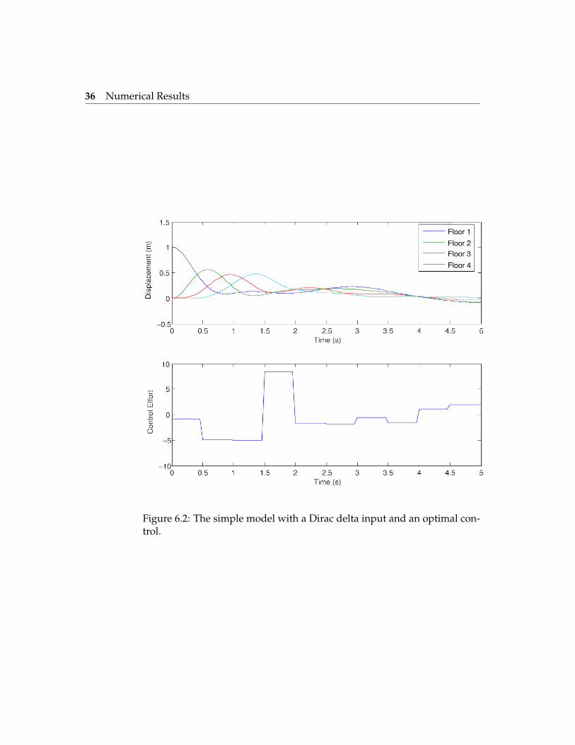
The simplest case, the building with four stories and one control, was testedfirst using the configuration described above. In the simulations, a smalldisplacement was given to the bottom floor to simulate a Dirac delta inputfrom the earthquake. Figure 6.1 shows how the system behaved when nocontrol was given to the system. Note that the floors continue to oscillateout of phase with each other, which causes significant stress on the build-ing’s structure. Additionally, the floors are barely damped by the naturaldamping coefficient and the building is listing to the right. In contrast,Figure 6.2 shows the behavior of the building with an optimal control de-termined by Miser3. Note that now the floors are oscillating in phase witheach other after the large spike at time t = 1.5. This time corresponds withwhen the wave travelling from the first floor reaches the fouth floor. It cantherefore be surmised that at this point, all of the energy of the control wasspent preventing the top floor from swinging back and sending a rippleback down the building. The energy of the control input is cancelling thevibrational energy of the building, resulting in a large damping effect.

Movies were constructed that showed how the building progressed intime, but they cannot included in this thesis.

6.3 Results for Multiple Stories

The numerical results for buildings with multiple stories could not be com-pleted by the time this thesis was due. However, preliminary results sug-gest that buildings with reasonably close height to the original four-storybuilding behave similarly and have similar optimal controls. Results forbuildings that are very large are not available.

Results for Multiple Stories 35

Figure 6.1: The simple model with a Dirac delta input and no control.

36 Numerical Results

Figure 6.2: The simple model with a Dirac delta input and an optimal con-trol.

Chapter 7

Discussion and Future Work

Several problems envisioned for this thesis could not be completed in time.Including the full numerical results for multiple stories, other ideas thatwere not fully developed have been listed here.

7.1 Linear Controls

The application of linear control usually suggests the use of bang-bang typesolutions. These solutions are well suited to regulator-type problems, sincethey can be physically realized using relays and other simple electroniccircuitry. However, linear controls offer some problems for mathematicalanalysis in the case where bang-bang controls are not the optimal solutionto the problem.

Using Pontryagin’s minimization principle given in the introduction,we can find the switching point of an objective functional given in the form

J =∫ t f

0Q~x + R~u dt

by finding conditions on the adjoint variables λi when they cross certainthresholds. However, if the adjoint variables stay at the switching points,then the system is called singular and an optimal control must be found bydifferent means. In general, this means a manual numerical search of allthe possible controls in the switching region.

If the existence of a bang-bang type solution could be demonstrated forthe model given in Chapter 2, then linear controls would offer a highly-intuitive objective functional that generates a control that is easy to imple-ment in actual buildings. However, singular controls have questionable

38 Discussion and Future Work

applicability, due to their extreme sensitivity to system parameters, and aretherefore far less desirable.

7.2 Continuous Model

In the above chapters, the discretized model was developed where eachfloor was represented with a lumped mass. To characterize the currentstate of the system, the position and velocity were recorded in the statevector ~x which allowed the dynamics of the system to be completely de-scribed by the vector. The advantage of this technique is that it allows theprevious state of the system to be ignored, as all future states of the systemare entirely described by the current state vector.

However, the discretization of the building involved a significant ap-proximation of the building motion. Although discretization is the mostcommon method used in structural control and simulation, as explained inChapter 1, continuous models still allow a finer-grained analysis of systembehavior. As described in the introduction, a continuous model that ap-proximates the structure with the mass of the building evenly distributedis an unphysical approximation. But, by applying a mass density functionρ(y) to the system, a partial differential equation (PDE) can be derived thatdescribes the movement of the building in space and time.

7.2.1 Mathematical Development

Separating the mass of the building vertically into chunks dy, we need tofind the reaction forces between the chunk at vertical position y and y + dy.Obviously, the reaction forces used in the discretized model need to beadapted for use with the differentials. Loosely, this can be accomplishedby comparing the values of u(y, t) and u(y + dy, t), as well as the pairut(y, t) and ut(y + dy, t) corresponding to the spring and damper forces,respectively. For the damper force, we would want the force applied to thesegment dy to be

Fd = c limdy→0

ut(y + dy, t)− ut(y, t)dy

= cuty(y, t)

while the spring force needs to account for hysteretic effects.Once the forces on each segment dy have been found, we can find the

acceleration of the chunk by Newton’s second law of motion, that dF =dm · a, so that the acceleration of the chunk is the forces divided by themass density function ρ(y).

Future Work and Conclusions 39

7.3 Future Work and Conclusions

This thesis focused on deterministic optimal control as applied to an apart-ment building. However, the system under consideration exhibits wildchaotic behavior with only a few state variables. Future mathematiciansshould consider using stochastic control rather than deterministic methodsto deal with the uncertainty in measurement and position. This predic-tion matches the efficiency of fuzzy controls in implementations of thesedevices.

The first semester began with a review of optimal control theory. Dur-ing the summer, I worked with profs. Gu and de Pillis on a tumor mod-eling project that used optimal control theory to find optimal solutions fortreatment of malignant tumors. Using this background, I researched fur-ther into optimal control and found sources related to structural controland optimization. The model presented in [6] was checked and explainedin Chapter 2, along with discussion and descriptions of the terms. Then,using the procedure developed during the summer and applying theoremsfrom Fleming and Rishel [2], Professor Gu and I proved the existence ofthe optimal control when the objective functional for quadratic objectivesin state and control. Demonstrating the existence of the objective controlwas the chief result of the semester.

Although preliminary work was completed in the first semester on thenumerical results, these were mainly developed in the second semester.The code was (eventually!) fixed and the building began to behave cor-rectly half-way through the semester. After these results, I showed defini-tively that the optimal control was reducing damage dealt to the build-ing for Dirac earthquakes; however, the rapid oscillations of sinusoidalearthquakes require large knot sets that are difficult to handle numerically.There are several parts of the thesis near completion that would be excel-lent projects for interested students.

Bibliography

[1] Fabio Casciati and Timothy Yao. Comparison of strategies for the activecontrol of civil structures. In First World Conference on Structural Control,volume 1, pages WA1–3–WA1–12, 1994.

This source introduces a basic sources and the state of theart in active control as of 1994. Different control strategiesare introduced, including state feedback linearization usingLQ, H2, and H∞ controls. The text questions the usefulnessof state feedback linearization as a control scheme, and sug-gests that predictive control, full nonlinear optimal regula-tor techniques, and sliding mode control are stronger controlmethods. The text suggests that both nonlinear optimal con-trol and sliding mode control are promising but are not gen-eral enough for wide applicability. The text also introducesa few control techniques such as neural network control andfuzzy control, which are unrelated to my thesis topic.

[2] Wendell H. Fleming and Raymond W. Rishel. Deterministic and Stochas-tic Optimal Control. Springer-Verlag, 1975.

Fleming and Rishel introduce the basic theorems and theorynecessary to prove the existence of an optimal control. Theybegin with definitions and the analysis of a general optimiza-tion problem, and then move into more complicated deter-ministic and stochastic optimal control theory. For my thesis,I am concerned with the chapter describing the existence anduniqueness theorems for an optimal control for different opti-mal control problems. The main theorem is given in the intro-duction of this thesis without proof, although one is suppliedin Fleming and Rishel.

42 Bibliography

[3] R. E. Kalman. Contributions to the theory of optimal control. Bol. Soc.Mat. Mex., 4:102–119, 1960.

This is the classic paper that details the state of the art in con-trol theory as of 1960. Kalman introduces the theory so that itis applicable to a general control theory problem with an ar-bitrary objective functional; however, most of the techniqueshe gives later are limited to situations with quadratic termsin the functional. Kalman introduces the Riccati equation andits application to find the coefficients for feedback in a linearcontrol system.

[4] J. J. Levin. On the matrix riccati equation. Proceedings Am. Math. Soc.,10:519–524, 1959.

Levin introduces several general results about the Riccatiequation in English.

[5] William T. Reid. A matrix differential equation of riccati type. Am. J.Math., 68:237–246, 1946.

Reid finds solutions to the Riccati differential equation andapplies the results to differential equations and the calculusof variations (and so, to control theory).

[6] Akira Sone, Shizuo Yamamoto, and Arata Masuda. Sliding mode con-trol for building using tuned mass damper with pendulum and levermechanism during strong earthquake. In Second World Conference onStructural Control, pages 531–540, 1998.

Sone et. al. form the foundation of the research performedin this thesis. They introduce the model used in this paper,which is a 4-story apartment building with a tuned massdamper on the top floor. They develop the model introducedin the first section of this thesis, which they use to simulatethe building during the earthquake and develop a slidingmode controller to minimze the oscillations.

[7] Ravi Shanker Thyagarajan. Modeling and Analysis of Hysteretic Struc-tural Behavior. PhD thesis, California Institute of Technology, Pasadena,California, 1989.

Thyagarajan introduces the different types of structural hys-teresis that are used in models for structural analysis and

Bibliography 43

controls. He differentiates between state space representa-tions and representations with memory. He also demon-strates that the more complicated models do not necessar-ily behave closer to their physical counterparts. Thyagarajanalso introduces the bilinear hysteretic model used in this the-sis.

[8] Dennis G. Zill and Michael R. Cullen. Differential Equations withBoundary-Value Problems. Brooks/Cole, 2001.

Zill and Cullen describe basic ordinary differential equationstheory and provide methods for solving systems of ordinarydifferential equations. In particular, they describe the methodof variation of parameters.