Optimal capture and sequestration from the carbon

emission �ow and from the atmospheric carbon stock with

heterogeneous energy consuming sectors

Jean-Pierre Amigues∗, Gilles La�orgue†

and

Michel Moreaux‡

May 10, 2010

Abstract

We characterize the optimal exploitation paths of two primary energy resources.

The �rst one is a non-renewable polluting resource, the second one a pollution-free

renewable resource. Both resources can supply the energy needs of two sectors. Sector

1 is able to reduce the potential carbon emissions generated by its non-renewable

energy consumption at a reasonable cost while sector 2 cannot. Another possibility

is to capture the carbon spread in the atmosphere but at a signi�cantly higher cost.

We assume that the atmospheric carbon stock cannot exceed some given ceiling and

that this constraint is e�ective. We show that there may exist paths along which it is

optimal to begin by fully capturing the sector 1's potential emission �ow before the

ceiling constraint begins to be e�ective. Also there may exist optimal paths along

which both capture devices have to be activated, in which case the potential emission

�ow of sector 1 is �rst fully abated and next the society must resort to the atmospheric

carbon reducing device.

Keywords: Fossil resource, Carbon stabilization cap, Heterogeneity, CCS, Air

capture.

JEL classi�cations: Q31, Q32, Q41, Q42, Q54, Q58.

∗Toulouse School of Economics (INRA and LERNA). E-mail address: amigues@toulouse.inra.fr†Corresponding author. Toulouse School of Economics (INRA-LERNA). 21 allée de Brienne, 31000

Toulouse, France. E-mail address: gla�org@toulouse.inra.fr. We are grateful to Valérie Nowaczyk fore�cient technical assistance.‡Toulouse School of Economics (IDEI and LERNA). E-mail address: mmichel@cict.fr.

1

1 Introduction

As recommended by the Intergovernmental Panel on Climate Change, abatement technolo-

gies must be used to reduce the anthropogenic carbon dioxide emissions in a climate change

mitigation objective (IPCC, 2007). Among all the alternatives, a particular interest should

be given to the carbon capture and sequestration (CCS) (IPCC, 2005). CCS technology

consists in �ltering CO2 �uxes at the source of emission, that is, in fossil energy-fueled

power plants, by use of scrubbers installed near the top of chimney stacks. The carbon

would be sequestered in reservoirs, such as exhausted salt and coal mines, depleted oil and

gas �elds or deep saline aquifers.

Even if the e�ciency of such a technology as well as the potential capacities of such

carbon sinks are still under assessment, current engineering estimates suggest that CCS

could be a credible cost-e�ective approach for eliminating most of the emissions from

coal and natural gas power plants (MIT, 2007). Along this line of arguments, Islegen and

Reichelstein (2009) point out that CCS has considerable potential to reduce CO2 emissions

at a social cost that most economists would consider as reasonable, given the social costs

of carbon emissions predicted for a business-as-usual scenario without regulation. For

regulated scenarios, CCS is also intended to have a major role in limiting the e�ective

carbon tax, that is, the market price for CO2 emission permits under a cap-and-trade

system. In that case, the crucial point is to estimate how far would the CO2 price have

to rise before the operator of power plants would �nd it advantageous to install CCS

technology rather then buy emission permits or pay the carbon tax. McKinsey & Company

(2007) estimates a break-even price, that is a carbon price from which CCS becomes an

economically viable alternative, in the range of $30-45 for coal-�re plants. This price rises

to at least $60 per tonne of CO2 in the case of power plants running on natural gas.

However, geologic CCS presents the disadvantage to apply to the sole large point sources

of pollution such as power plants or huge manufacturings. This technology is prohibitively

costly to �lter for instance the CO2 emissions from transportation as far as the energy

input is gasoline or kerosene1, small residence heating or scattered agricultural activities.

Hence, the ultimate device to abate carbon dioxide �uxes from any concentrated as well as

di�use sources would consist in capturing them directly from the atmosphere. Deliberately

expressing a double meaning, McKay (2009) claims about this alternative that "captur-

1Note that an electric railway system escapes this constraint.

2

ing carbon dioxide from thin air is the last thing we should talk about" (p.240). On the

one hand, the energy requirements for atmospheric carbon capture are so enormous that,

according to McKay, it seems actually almost absurd to talk about it. But on the other

hand, McKay argues that "we should talk about it, contemplate how best to do it, and fund

research into how to do it better, because capturing carbon from thin air may turn out to

be our last line of defense, if climate change is as bad as the climate scientists say, and

if humanity fails to take the cheaper and more sensible options that may still be available

today" (p.240).

Technically speaking, removing carbon from the atmosphere can be achieved in di�erent

ways. The most obvious approach consists in exploiting the process of photosynthesis. A

close idea can be transposed to the oceans. To make them able to capture carbon faster

then normal, phytoplankton blooms can be stimulated by fertilizing some oceanic iron-

limited regions. A third way is to enhance weathering of rocks, that is to pulverize rocks

that are capable of absorbing C02, and leave them in the open air. This idea can be pitched

as the acceleration of a natural process. Unfortunately, as claimed by Barrett (2009), the

e�ects of all these devices are di�cult to verify, their potential is limited in any event, and

there are concerns about some unknown ecological consequences.

A probably most credible way of sucking carbon from thin air is to use a chemical

process. This involves a technology that brings air into contact with a chemical "sorbent"

(an alkaline liquid). The sorbent absorbs CO2 in the air, and the chemical process then

separates out the CO2 and recycles the sorbent. Finally, the captured CO2 is stored in

geologic deposits, just like the CCS from power plant described above. However, chemical

air capture is expensive. Estimates of marginal cost range from $100-200/tCO2, which

is larger than the cost of alternatives for reducing emissions such as power plant CCS.

They are also larger than current estimates of the social cost of carbon, which range from

about $7-85/tCO2. But, as concluded by Barrett (2009), bearing the cost of chemical air

capture can become pro�table in the future under constraining cap-and-trade scenarios.

Furthermore, we may hope that the cost will decrease, thanks to R&D and learning by

doing.

In the present study, we address the question of the heterogeneity of energy users

regarding the way their carbon footprint can be reduced. We then consider two abatement

technologies and two sectors. The �rst technology is a conventional emission abatement

3

device (CCS) which is available at a marginal cost assumed to be socially acceptable.

However, this abatement technology cannot apply to carbon emissions from any type of

activity, but only from large point sources of emissions. The second technology directly

captures carbon in the atmosphere. Its marginal cost is highly costlier than the emission

capture technology, but it allows to reduce carbon from any sources since the capture

process and the generation of emissions are now disconnected. The �rst sector, in which

pollution sources are spatially concentrated, can abate its carbon emissions, but not the

second one since energy users are too small and too scattered. The ultimate way for abating

pollution is to directly capture carbon in the atmosphere. But since the atmosphere is a

public good, this kind of pollution reduction will also bene�t to sector 1. Whatever the

capture process, we assume that carbon is stockpiled into reservoirs whose size is very

large. Then, as in Chakravorty et al., (2006-b) this suggests a generic abatement scheme

of unlimited capacity2. Finally, energy in each sector can be supplied either by a carbon-

based fossil fuel, contributing to climate change (oil, cal, gas), or by a carbon-free renewable

and non biological resource such, as solar energy.

Using a standard Hotelling model for the non-renewable resource and assuming that the

atmospheric carbon stock should not exceed some critical threshold, we then characterize

the optimal time path of sectoral energy prices, sectoral energy consumptions, emission

and atmospheric abatements. The key results of the paper are: i) Irrespective of the

availability of the air capture technology, it may happen that it is optimal for the �rst

sector to abate its carbon emissions before the atmospheric carbon concentration cap is

attained. ii) Since this type of carbon capture is unable to �lter the emissions from the

second sector, it is also optimal for the �rst sector to abate the totality of its own emissions,

at least at the beginning. These two �rst results are at variance with Chakravorty et al.

(2006-b), La�orgue et al. (2008-a) and (2008-b) who consider a single sector using energy

and a single abatement technology. iii) The atmospheric carbon capture is only used when

the atmospheric carbon stock reaches the ceiling, maintaining the stock at its critical level.

Hence the �ow of carbon captured in the atmosphere is lower than the emission �ow of the

second sector.

The paper is organized as follows. Section 2 presents the model. In section 3, we lay

down the social planner program and we derive the optimality conditions. In section 4,

2The question of the size of carbon sinks and of the time pro�le of their �lling up is addressed byLa�orgue et al. (2008-a, 2008-b).

4

we examine the restricted problem in which only the emission carbon capture device is

available. In section 5, we examine how the model reacts when the atmospheric carbon

capture technology is introduced. We also investigate the time pro�le of the optimal carbon

tax as well as, for each sector, the total burden induced by the mitigation of their emissions.

Finally, we brie�y conclude in section 6.

2 Model and notations

Let us consider a stationary economy with two sectors, indexed by i = 1, 2, in which the

instantaneous gross surplus derived from energy consumption are the same. For an identical

energy consumption in the two sectors, q1 = q2 = q, the sectoral gross surplus u1(q) and

u2(q) are such that: u1(q) = u2(q) = u(q). We assume that this common function u

satis�es the following standard assumptions. u : R+ → R+ is a function of class C2,

strictly increasing, strictly concave and verifying the Inada conditions: limq↓0 u′(q) = +∞

and limq↑+∞ u′(q) = 0. We denote by p(q) the sectoral marginal gross surplus function

and by qd(p) = p−1(p), the sectoral direct demand function.

In each sector, energy can be supplied by two primary natural resources: a dirty non-

renewable resource (let say oil for instance) and a carbon-free renewable resource (let say

solar energy).

Let us denote by X0 the initial oil endowment of the economy, by X(t) the remain-

ing part of this initial endowment at time t, and by xi(t), i = 1, 2, the instantaneous

consumption �ow of oil in sector i at time t, so that:

X(t) = −[x1(t) + x2(t)], with X(0) ≡ X0 and X(t) ≥ 0 (1)

xi(t) ≥ 0, i = 1, 2. (2)

The delivery cost of oil is the same for both sectors. We denote by cx the corresponding

average cost, assumed to be constant and hence equal to the marginal cost. The delivery

cost includes the extraction cost of the resource, the cost of industrial processing (re�ning

of the crude oil) and the transportation cost, so that the resource is ready for use by the

consumer in the concerned sector. To keep matter as simple as possible, we assume that no

oil is lost during the delivery process. Equivalently, the oil stock X(t) may be understood

as measured in ready for use units.

5

Let Z(t) be the stock of carbon within the atmosphere at time t, and Z0 be the initial

stock, Z0 ≡ Z(0). We assume that a carbon cap policy is prescribed to prevent catastrophic

damages which would be in�nitely costly. This policy consists in forcing the atmospheric

stock to stay under some critical level Z, with Z > Z0.

The atmospheric carbon stock is fed by carbon emission �ows resulting from the use

of oil. Let ζ be the quantity of carbon which would be potentially released by unit of oil

consumption whatever the sector in which the oil is used. Thus, the gross pollutant �ow

amounts to ζ[x1(t) + x2(t)]. However, this gross emission �ow can be abated before being

released into the atmosphere. We assume that emissions from sector 1 can be abated, but

not emissions from sector 2 (or at a prohibitive cost). Emission abatement by carbon cap-

ture and sequestration (CCS) can be achieved when burning oil is spatially concentrated,

as it is the case for instance in the electricity or cement industries, which are good examples

of sector 1's activities. At the other extreme of the spectrum, i.e. in sector 2, there exists

some activities with prohibitively costing emission captures since users are too small or

too scattered. Transportation by cars, trucks and diesel train are good examples of sector

2's industry3.

Let se(t) be this part of carbon emissions from sector 1 which is captured and se-

questered at some average cost ce, assumed to be constant. Thus the net pollution �ow

issued from sector 1 amounts to:

ζx1(t)− se(t) ≥ 0, se(t) ≥ 0. (3)

In sector 2, the net pollution �ow amounts to ζx2(t).

Carbon emission capture is not the unique way to reduce the atmospheric carbon con-

centration. The other process consists in capturing the carbon present in the atmosphere

itself. We denote by sa(t) the instantaneous carbon �ow which is abated owing to this

second device, and by ca the corresponding average cost, also assumed to be constant.

Although atmospheric carbon capture seems technically feasible, it is proved to be more

costly than emission capture: ca > ce.4 The only constraint on this capture �ow is:

sa(t) ≥ 0 (4)

3Note that electric traction trains could be good examples of sector 1 users.4Classical devices allowing for the carbon capture and sequestration from the atmosphere consists in

increasing the forestlands and changing the agricultural processes. This is not the type of device weconsider in the present paper.

6

Last, there is also some natural self regeneration e�ect of the atmospheric carbon stock.

We assume that the natural proportional rate of decay, denoted by α > 0, is constant.

Taking into account all the components of the dynamics of Z(t) results into:

Z(t) = ζ[x1(t) + x2(t)]− [sa(t) + se(t)]− αZ(t), Z(0) ≡ Z0 < Z (5)

Z − Z(t) ≥ 0. (6)

When the atmospheric carbon stock reaches its critical level, i.e. when Z(t) = Z, and

absent any active capture policy, i.e. sa(t) = se(t) = 0, then the total oil consumption

x(t) ≡ x1(t)+x2(t) is constrained to be at most equal to x, where x is solution of ζx−αZ =

0, that is:

x =α

ζZ.

We assume that it may be optimal to abate the pollution for delaying the date of arrival

at the critical threshold and for relaxing the constraint on the oil consumption �ow, that

is:

cx + ca < u′(x)⇒ cx + ce < u′(x).

The alternative energy source is supplied by the carbon-free renewable resource, the

solar energy. We denote by yi(t) the solar energy consumption in sector i, i = 1, 2, and by

cy the average delivery cost of this alternative energy. Because cx and cy both include all

the costs necessary to deliver a ready for use energy unit to the potential users, then both

resources may be seen as perfect substitutes for the consumers, so that we may de�ne the

aggregate energy consumption of sector i as qi = xi + yi, i = 1, 2, as far as the costs cx

and cy are incurred.

The average cost cy is assumed to be constant, the same for both sectors, and higher

than u′(x/2). This last condition implies that the optimal energy consumption paths can

be split into two periods: a �rst one during which only oil is consumed and a second one

during which only solar energy is used. We also have to assume that the natural �ow of

available solar energy, denoted by yn, is large enough to supply the energy needs in both

sectors during the second period described above. Let y be the sectoral energy consumption

that it would be optimal to consume at the marginal cost cy, that is y = qd(cy) for which

u′(y) = cy. Then we assume that yn > 2y. Under this assumption, no rent has ever to be

imputed for using the solar energy. Thus the only constraint on yi(t) having to be taken

into account along any optimal path is a non-negativity constraint:

yi(t) ≥ 0, i = 1, 2. (7)

7

Finally, the instantaneous social rate of discount, denoted by ρ, ρ > 0, is assumed to

be constant over time.

3 Social planner problem and optimality conditions

The problem of the social planner consists in maximizing the sum of the discounted net

current surplus. Let (P ) be this program:

(P ) maxsa,se,xi,yi,i=1,2

∫ ∞0{u [x1(t) + y1(t)] + u [x2(t) + y2(t)]− cx [x1(t) + x2(t)]

−cy [y1(t) + y2(t)]− casa(t)− cese(t)} e−ρtdt

subject to (1)-(7).

Let us denote by λX the costate variable of the state variable X, by λZ minus the

costate variable of the state variable Z, by γ's the Lagrange multipliers associated with

the non-negativity constraints on the command variables, and by ν the Lagrange multiplier

associated with the ceiling constraint on Z. As usually done in this kind of problem, we do

not take explicitly into account the non-negativity constraint on X. Thus we may write

the current value Lagrangian L of problem (P ) as follows:

L(t) = u [x1(t) + y1(t)] + u [x2(t) + y2(t)]− cx [x1(t) + x2(t)]− cy [y1(t) + y2(t)]

−casa(t)− cese(t)− λX(t) [x1(t) + x2(t)]

−λZ(t) {ζ [x1(t) + x2(t)]− [sa(t) + se(t)]− αZ(t)}

+ν(t)[Z − Z(t)

]+∑i

γxi(t)xi(t) +∑i

γyi(t)yi(t)

+γsa(t)sa(t) + γse(t)se(t) + γse(t) [ζx1(t)− se(t)]

The �rst-order conditions relative to the command variables are:

∂L∂x1

= 0 ⇒ u′[x1(t) + y1(t)] = cx + λX(t) + ζ[λZ(t)− γse(t)]− γx1(t) (8)

∂L∂x2

= 0 ⇒ u′[x2(t) + y2(t)] = cx + λX(t) + ζλZ(t)− γx2(t) (9)

∂L∂yi

= 0 ⇒ u′[xi(t) + yi(t)] = cy − γyi(t), i = 1, 2 (10)

∂L∂sa

= 0 ⇒ ca = λZ(t) + γsa(t) (11)

∂L∂se

= 0 ⇒ ce = λZ(t)− γse(t) + γse(t) (12)

8

The associated complementary slackness conditions are:

γxi(t) ≥ 0, xi(t) ≥ 0 and γxi(t)xi(t) = 0, i = 1, 2 (13)

γyi(t) ≥ 0, yi(t) ≥ 0 and γyi(t)yi(t) = 0, i = 1, 2 (14)

γsa(t) ≥ 0, sa(t) ≥ 0 and γsa(t)sa(t) = 0 (15)

γse(t) ≥ 0, se(t) ≥ 0 and γse(t)se(t) = 0 (16)

γse(t) ≥ 0, ζx1(t)− se(t) ≥ 0 and γse(t)[ζx1(t)− se(t)] = 0 (17)

The dynamics of the costate variables must satisfy:

λX = ρλX −∂L∂X

⇒ λX(t) = ρλX(t) (18)

λZ = ρλZ −∂L∂Z

⇒ λZ(t) = (ρ+ α)λZ(t)− ν(t) (19)

together with the complementary slackness condition:

ν(t) ≥ 0, Z − Z(t) ≥ 0 and ν(t)[Z − Z(t)] ≥ 0. (20)

Last, the transversality conditions take the following forms:

limt↑∞

e−ρtλX(t)X(t) = 0 (21)

limt↑∞

e−ρtλZ(t)Z(t) = 0 (22)

Remarks:

1. The shadow marginal value of the stock of oil, or mining rent, λX(t), must grow at

the social rate of discount ρ. From (18), we get:

λX(t) = λX0eρt, λX0 ≡ λX(0). (23)

Thus the transversality condition (21) reduces to:

λX0 limt↑∞

X(t) = 0. (24)

If oil is to have some value, λX0 > 0, then it must be exhausted along the optimal

path.

2. Concerning the shadow marginal cost of the atmospheric carbon stock, λZ(t), note

that before the date tZ at which the ceiling constraint is beginning to be active, we

must have ν(t) = 0 since Z − Z(t) > 0. Then (19) reduces to λZ = (ρ + α)λZ so

that:

t < tZ ⇒ λZ(t) = λZ0e(ρ+α)t, λZ0 ≡ λZ(0). (25)

9

Once the ceiling constraint is no more active and forever, λZ(t) = 0. Thus, denoting

by tZ the latest date at which Z(t) = Z, we get:

t > tZ ⇒ λZ(t) = 0. (26)

In order to simplify the notations in the next sections, it is useful to de�ne the following

prices or full marginal costs and the corresponding sectoral consumption levels for which

the F.O.C's (8) and (9) relative to x1(t) and to x2(t), respectively, are satis�ed5.

• Price or full marginal cost of oil and sectoral oil consumption before the ceiling and

absent any abatement, whatever the sector under consideration:

p1(t, λX0 , λZ0) ≡ cx + λX0eρt + ζλZ0e

(ρ+α)t (27)

q1(t, λX0 , λZ0) ≡ qd(p1(t, λX0 , λZ0)

)(28)

• Price or full marginal cost of oil for consumption in sector 1 given that emissions

from this sector are fully or partially abated, i.e. se(t) > 0, and corresponding oil

consumption of sector 1:

p2e(t, λX0) ≡ cx + λX0e

ρt + ζce (29)

q2e(t, λX0) ≡ qd

(p2e(t, λX0)

)(30)

• Price or full marginal cost of oil for consumption in sector 2 given that some part of

the atmospheric carbon stock is captured, sa(t) > 0, and corresponding consumption

in this sector:

p2a(t, λX0) ≡ cx + λX0e

ρt + ζca (31)

q2a(t, λX0) ≡ qd

(p2a(t, λX0)

)(32)

• Price or full marginal cost of oil once the ceiling constraint Z − Z(t) ≥ 0 is no more

active and forever, and corresponding sectoral consumptions, whatever the sector:

p3(t, λX0) ≡ cx + λX0eρt (33)

q3(t, λX0) ≡ qd(p3(t, λX0)

)(34)

This last case corresponds to a pure Hotelling regime.

5The upper indexes n = 1, 2, 3 correspond to the order in which the price pn and the quantity qn areappearing along the optimal path. If both pn(t, ...) and pn+m(t′, ...) are appearing along the same path,then it implies that t < t′.

10

Problem solving strategy:

To solve the social planner problem (P ), we proceed as follows. First, we check whether

the most costly device to capture the carbon has ever to be used. The test consists in

solving the social planner problem assuming that the atmospheric carbon capture device is

not available. This is inducing some path of atmospheric carbon shadow cost λZ(t). Then:

- either this shadow cost is permanently lower than the marginal cost of atmospheric

carbon capture, that is λZ(t) < ca for any t ≥ 0, and then the atmospheric carbon capture

device has never to be used because too costly;

- or there exists some time interval during which λZ(t) is higher than ca so that, in

this case, the atmospheric carbon capture device must be activated since the loss in the

marginal net surplus induced by not using it is higher than its marginal cost of use.

4 Optimal policy without atmospheric carbon capture device

This kind of policies have been investigated and characterized in Chakravorty et al. (2006-

a, 2006-b) and in La�orgue et al. (2008-a, 2008-b), but for economies in which any potential

emissions can be captured and sequestered irrespective of the oil consumption sector. Thus,

in their models, there is a single consumption sector, similar to the sector 1 of the present

model.

Two important conclusions of these studies are that: i) it is never optimal to abate

the potential �ow of emissions before attaining the critical level Z of atmospheric carbon

concentration; ii) along the phase at the ceiling during which it is optimal to abate, only

some part of the potential emission �ow must be abated; because abating is never optimal

excepted during this phase, then it is never optimal to fully abate the potential �ow of

emissions along the optimal path.

As we shall show, it may happen in the present context that: i) abating the potential

emissions of the sector 1 has to begin before the ceiling level Z is attained; ii) when it is

optimal to begin to capture the sector 1 potential emissions, before the ceiling is attained,

then it is optimal to capture its whole potential emission �ow.

11

4.1 Restricted social planner problem

Assuming that the atmospheric carbon capture technology is not available, the social

planner problem reduces to the following restricted problem (R.P ):

(R.P ) maxse,xi,yi,i=1,2

∫ ∞0{u [x1(t) + y1(t)] + u [x2(t) + y2(t)]− cx [x1(t) + x2(t)]

−cy [y1(t) + y2(t)]− cese(t)} e−ρtdt

subject to (1), (2), (3), (6), (7) and:

Z(t) = ζ[x1(t) + x2(t)]− se(t)− αZ(t), Z(0) = Z0 < Z (35)

The current value Lagrangian of (R.P ), denoted by LR, writes now:

LR(t) = u [x1(t) + y1(t)] + u [x2(t) + y2(t)]− cx [x1(t) + x2(t)]− cy [y1(t) + y2(t)]

−cese(t)− λX(t) [x1(t) + x2(t)]− λZ(t) {ζ [x1(t) + x2(t)]− se(t)− αZ(t)}

+ν(t)[Z − Z(t)

]+∑i

γxi(t)xi(t) +∑i

γyi(t)yi(t)

+γse(t)se(t) + γse(t) [ζx1(t)− se(t)] .

The new F.O.C's relative to the command variables, except sa, together with the asso-

ciated complementary slackness conditions, are the same then the ones of the unrestricted

problem (P ), namely (8)-(12) and (13)-(17). Also the equations (18) and(19) determining

the dynamics of the costate variables, the complementary slackness condition (20) on ν

and the associated transversality conditions (21) and (22) when t tends to in�nity, must

hold.

We can conclude that remarks 1 and 2 of the previous section 3 also hold in the present

restricted context.

4.2 Optimal paths along which it is optimal to capture and sequester

before being at the ceiling

Let us assume that the initial oil endowment is large enough to justify some period at

the ceiling during which Z(t) = Z, and that there exists some period during which the

emissions of sector 1 are wholly or partially abated, se(t) > 0. Two kinds of such paths

can be optimal, depending on whether sector 1's emissions have to be captured from the

beginning of the planning horizon or later.

12

4.2.1 Optimal paths along which it is not optimal to abate from the beginning

Such paths are illustrated in the Figure 1 below.

[Figure 1 here]

The optimal price path depicted in Figure 1 is a seven phases path. Denoting by pi(t),

for i = 1, 2, the price � or full marginal cost � of oil for sector i, these phases are the

following:

- Phase 1, before the ceiling and without abatement: [0, te)

During this phase, the oil price is the same for each sector and it is given by p1(t) = p2(t) =

p1(t, λX0 , λZ0). The existence of such a phase requires that λZ0 < ce, so p1(t, λX0 , λZ0) <

p2e(t, λX0), that is capturing sector 1's emissions would be too costly. p1(t, λX0 , λZ0) −

p2e(t, λX0) = ζ

[λZ0e

(ρ+α)t − ce]< 0, is increasing so that supporting the marginal shadow

cost of the atmospheric carbon stock, λZ(t) = λZ0e(ρ+α)t, is less costly than abating, that

is supporting the marginal cost of abating the sector 1's emissions, ce.

The oil consumption of each sector is given by x1(t) = x2(t) = q1(t, λX0 , λZ0).

The common oil price p1(t, λX0 , λZ0) is increasing at an instantaneous rate which is

higher than the rate of growth of p2e(t, λX0). At the end of the phase, denoted by te, both

prices are equated p1(t, λX0 , λZ0) = p2e(t, λX0).

Note that, since p1(t) = p2(t) < u′(x) and Z0 < Z, then during this phase both x1(t)

and x2(t) are higher than x so that Z(t) is increasing. However, the existence of this phase

requires that, at its end, Z(t) is lower than the critical level Z: Z(te) < Z.

- Phase 2, before the ceiling with full abatement of sector 1's emissions: [te, tZ)

From te onwards, we have p2e(t, λX0) < p1(t, λX0 , λZ0). Thus it is now strictly less costly

for sector 1 to abate than not to abate, hence p1(t) = p2e(t, λX0), implying that x1(t) =

q2e(t, λX0).6 Moreover, since the inequality is strict then the potential sector 1's emissions

are fully abated: se(t) = ζx1(t).6Note that during such a phase, because se(t) > 0 then γse(t) = 0, so that from (12) we obtain:

λZ(t) = ce + γse(t).

Substituting for λZ(t) in (8) and taking into account that x1(t) > 0, hence γx1(t) = 0, and y1(t) = 0, weget:

u′ (x1(t)) = cx + λX0eρt + ζce,

from which we conclude that p1(t) = p2e(t, λX0) and x1(t) = q2e(t, λX0).

13

Sector 2 is not able to abate its emissions and it must support the carbon shadow

cost ζλZ0e(ρ+α)t per unit of burned oil, so that p2(t) = p1(t, λX0 , λZ0) and x2(t) =

q1(t, λX0 , λZ0).

Note that, during this phase, since Z(te) < Z and p2(t) < u′(x), then x2(t) > x and

the atmospheric carbon stock increases. Finally, since p2(t) > p1(t), the �rst of these two

prices reaching u′(x) is p2(t). However, in order that sector 2's consumption begins to be

blockaded at t = tZ , we must have simultaneously p2(t) = u′(x) and Z(t) = Z at the end

of the phase.

- Phase 3, at the ceiling with sector 2's oil consumption blockaded and sector

1's emissions fully abated: [tZ , t)

During this phase, the oil price in sector 2 is given by p2(t) = u′(x) and the oil consumption

of this sector is set to the maximum consumption level allowed by the ceiling constraint,

i.e. x2(t) = x. Note that this implies that λZ(t) = [u′(x)− p3(t, λX0)]/ζ is decreasing over

time during the phase7.

Since p2e(tZ , λX0) < u′(x), then ce < λZ(t) at the beginning of the phase. Then,

once again, abating emissions is proved to be less costly for sector 1 than supporting the

shadow cost of the atmospheric carbon stock. Consequently, the sector 1's emissions are

fully captured: se(t) = ζx1(t). Since p1(t) = p2e(tZ , λX0), we still have x1(t) = q2

e(t, λX0).

Given that sector 2's emissions are ζx2(t) = ζx, full abatement in sector 1 implies that,

during this phase at the ceiling, the atmospheric carbon stock stays at its critical level:

Z(t) = 0 and Z(t) = Z. Finally, p1(t) = p2e(t, λX0) is increasing during the phase. At the

end of the phase, p2e(t, λX0) = u′(x) or, equivalently, λZ(t) = ca.

- Phase 4, at the ceiling with partial abatement of sector 1's emissions: [t, te)

From time t onwards, p2e(t, λX0) becomes higher than u′(x). Thus, the only way to satisfy

simultaneously the F.O.C's (8) and (9) on the xi's is to set p1(t) = p2(t) = p2e(t, λX0),

which implies x1(t) = x2(t) = q2e(t, λX0) together with a partial abatement of sector 1's

emissions. As far as p2e(t, λX0) is staying under u′(x/2), then the potential emissions

amount to 2ζq2e(t, λX0) > ζx = αZ. As far as p2

e(t, λX0) is now higher than u′(x), then the

7Since the ceiling constraint is active, then ν(t) is strictly positive and su�ciently high so that λZ(t) =(ρ+ α)λZ(t)− ν(t) < 0.

14

potential emissions 2ζq2e(t, λX0) stays at a lower level than 2ζx, so that:

x < 2q2e(t, λX0) < 2x. (36)

In order to satisfy the atmospheric carbon constraint Z(t) = Z, it is su�cient to abate

this part se(t) of the sector 1's emissions for which Z(t) = 0. Thus we may have:

2ζq2e(t, λX0)− se(t) = ζx. (37)

Conditions (36) and (37) imply that:

se(t) = ζ[2q2e(t, λX0)− x

]< ζq2

e(t, λX0) = ζx1(t). (38)

Hence, during this phase, emissions from sector 1 are only partially abated and, since

q2e(t, λX0) is decreasing through time then the instantaneous rate of capture se(t) is also

decreasing. This solution may be optimal if and only if abating and supporting the shadow

marginal cost of the atmospheric carbon stock are resulting into the same full marginal

cost, that is if and only if λZ(t) is constant and equal to ce. Since sector 2 cannot abate

its emissions, it is supporting the marginal shadow cost of atmospheric carbon and the

condition p1(t) = p2(t) = p2e(t, λX0) = cx + λX0e

ρt + ζλZ(t) guarantees that λZ(t) = ce is

satis�ed8.

Since p2e(t, λX0) is increasing over time, there exists some date te at which p

2e(t, λX0) =

u′(x/2). At this date, x1(t) = x2(t) = x/2 and sector 1 ceases to capture its emissions,

se(t) = 0. From te onwards, we have p2e(t, λX0) > u′(x/2) so that the cost of capture of

sector 1's emissions becomes prohibitive.

- Phase 5, at the ceiling and without abatement of sector 1's emissions: [te, tZ)

Since abating the sector 1's emissions is now too costly, there is no more abatement and, in

order to not overshoot the critical atmospheric carbon level, we must have p1(t) = p2(t) =

u′(x/2) and x1(t) = x2(t) = x/2, so that Z(t) = 0.

During such a phase, λZ(t) = u′(x) − p3(t, λX0)/ζ is decreasing. The phase is ending

at time t = tZ when λZ(t) = 0, which implies that p3(t, λX0) > u′(x/2) for t > tZ .

8Again, because the ceiling constraint is e�ective then ν(t) > 0 and, in order that λZ(t) = 0, we have:ν(t) = (ρ+ α)λZ(t) = (ρ+ α)ce.

15

- Phase 6, pure Hotelling phase: [tZ , ty)

This phase is the last one during which energy needs are supplied by oil. This is a pure

Hotelling phase. The energy price is the same for the two sectors: p1(t) = p2(t) =

p3(t, λX0) > u′(x/2), also generating an identical oil consumption in the two sectors:

x1(t) = x2(t) < x/2⇒ x(t) < x.

Since x(t) < x and Z(t) = Z at the beginning of the phase, then Z(t) < Z for t > tZ

justifying the fact that now λZ(t) = 0 from tZ onwards9. Then λZ(t)Z(t) = 0 and the

transversality condition (22) is satis�ed.

During the phase, the price is ever increasing and there must exist some time t = ty

at which p3(t, λX0) = cy. At this time, this level of oil price makes the renewable resource

competitive. To be optimal, the switch from the pure Hotelling regime to a pure renewable

regime requires that, at time t = ty, X(t) = 0 so that from ty onwards λX(t)X(t) = 0

warranting that the transversality condition (21) relative to X is satis�ed.

- Phase 7, carbon-free renewable energy permanent regime: [ty,+∞)

From ty onwards, the economy follows a pure renewable energy regime which is free of

carbon emissions: p1(t) = p2(t) = cy, x1(t) = x2(t) = 0 and y1(t) = y2(t) = y. Since

xi(t) = 0, i = 1, 2, then Z(t) = −αZ(t) so that Z(t) is permanently decreasing down to 0

at in�nity: Z(t) = Z(ty)e−α(t−ty).

Determination of the characteristics of the optimal path:

The optimal path described above is parametrized by eight variables whose values have to

be determined: λX0 , λZ0 , te, tZ , t, te, tZ and ty. They are given as the solutions of the

following eight equations system.

- Balance equation of non-renewable resource consumption and supply:

2∫ te

0q1(t, λX0 , λZ0)dt+

∫ tZ

te

[q1(t, λX0 , λZ0) + q2

e(t, λX0)]dt

+∫ t

tZ

[q2e(t, λX0) + x

]dt+ 2

∫ te

tq2e(t, λX0)dt

+ [tZ − te] x+ 2∫ ty

tZ

q3(t, λX0)dt = X0. (39)

9However, note that Z(t) is not necessarily monotonically decreasing during this phase. What is sureis that there exists some critical time interval (tZ , tZ + ε), with ε positive and small enough, during whichZ(t) < 0. For t > tZ +ε, it may happen that Z(t) > 0. But, because x(t) < x, even if Z(t) were temporallyincreasing, it would not be able to go back to Z.

16

- Continuity of the carbon stock at time tZ :

Z0e−αtZ + 2ζ∫ te

0q1(t, λX0 , λZ0)e−α(tZ−t)dt

+ζ∫ tZ

te

q1(t, λX0 , λZ0)e−α(tZ−t)dt = Z. (40)

- Price continuity equations:

p1 (te, λX0 , λZ0) = p2e (te, λX0) (41)

p1 (tZ , λX0 , λZ0) = u′(x) (42)

p2e

(t, λX0

)= u′(x) (43)

p2e (te, λX0) = u′(x/2) (44)

p3 (tZ , λX0) = u′(x/2) (45)

p3(ty, λX0) = cy. (46)

Assuming a positive solution of system (39)-(46), then it is easy to check that all the

optimality conditions of the restricted problem (R.P ) are satis�ed. Reciprocally, it is clear

that there exists values of the parameters of the system cx, cy, ce, ζ, α and ρ together

with values of initial endowments of oil X0 and of atmospheric carbon stock Z0 such that

the path described above is the solution of the restricted problem (R.P ). However, other

solutions may exist.

4.2.2 Optimal paths along which it is optimal to abate from the beginning

Consider the optimal path characterized in the previous subsection 4.2.1 and some date t

between te and tZ (see Figure 1). At this time t:

- The stock of oil amounts to:

X(t) = X0 − 2∫ te

0q1(t, λX0 , λZ0)dt−

∫ t

te

q1(t, λX0 , λZ0)dt

−∫ t

te

q2e(t, λX0)dt. (47)

- The stock of atmospheric carbon is:

Z(t) = Z0e−αt + 2ζ∫ te

0q1(t, λX0 , λZ0)e−α(t−t)dt

+ζ∫ t

te

q1(t, λX0 , λZ0)e−α(t−t)dt+ ζ

∫ t

te

q2e(t, λX0)e−α(t−t)dt (48)

17

Assume that the oil endowment of the economy is X(t) instead of X0 and that the

initial atmospheric carbon stock is Z(t) < Z instead of Z0. Since in the present model

the solution of (R.P ) is time consistent, then the optimal price path restricted by this

new initial conditions (47) and (48) proves to be this part of the previous path beginning

at time t = t. More precisely, if pi(t), i = 1, 2, is the solution described in the previous

subsection 4.2.1, then the solution, denoted by pi(t), corresponding to the initial conditions

(47) and (48) is given by:

pi(t) = pi(t+ t), i = 1, 2. (49)

Now, the �rst phase (i.e. phase 1) before the ceiling and without emission abatement

is going out and sector 1's emissions must be captured from the beginning of the planning

horizon, that is from t.

4.3 Paths along which the oil prices path is the same for the two sectors

4.3.1 Paths along which it is optimal to abate sector 1's emissions

Example of such a path, solution of the restricted problem (R.P ), is illustrated in Figure

2 below.

[Figure 2 here.]

This kind of paths is characterized by the fact that, at time t = te at which p1(t, λX0 , λZ0) =

p2e(t, λX0), then the common value of these two prices is larger than u′(x) while Z(te) = Z

simultaneously.

Because Z0 < Z there must exist a �rst phase [0, te) during which the ceiling Z is not

yet attained and p1(t) = p2(t) = p1(t, λX0 , λZ0) < p2e(t, λX0), hence it is not optimal to

abate sector 1's emissions. At the end of this �rst phase, both p1(t, λX0 , λZ0) = p2e(t, λX0)

and Z(te) = Z so that te coincides with tZ .

The next phase [te, te) is a phase at the ceiling during which p1(t) = p2(t) = p2e(t, λX0).

As in the phase 4 of the previous case � [t, te) of the path illustrated in Figure 1 � because

sector 2 cannot abate its emissions, we must have λZ(t) = ce during the second phase

of the present path. Also because u′(x) < p2e(t, λX0) < u′(x/2), then only some part

of the sector 1's emissions have to be captured (cf. the above equation (38)), se(t) <

18

ζq2e(t, λX0) = ζx1(t), and the capture intensity se(t) diminishes. At the end of this phase,

p2e(t, λX0) = u′(x/2), x1(t) = x2(t) = x/2 and se(t) = 0.

The third phase [te, tZ) is still a phase at the ceiling but without capture of sector 1's

emissions: p1(t) = p2(t) = u′(x/2) and x1(t) = x2(t) = x/2. The phase is ending when

p3(t, λX0) = u′(x/2), that is when λZ(t) = 0. The fourth and �fth phases are respectively

the standard pure Hotelling phase [tZ , ty) and the pure renewable energy phase [ty,∞).

4.3.2 Paths along which it is never optimal to capture sector 1's emissions

When the abatement cost ce is very high, capturing is proved to never be an optimal

strategy. In this case, we get a four phases optimal price path as illustrated in Figure 3.

[Figure 3 here.]

In Figure 3, p2e(t, λX0) is higher than p1(t, λX0 , λZ0) along the whole time interval [0, tZ)

before the ceiling. Hence, it is never optimal to capture sector 1's emissions. Such optimal

paths have been characterized in Chakravorty et al. (2006-a, 2006-b).

5 Optimal policies requiring to activate both capture devices

In this section, we �rst determine the conditions under which it is optimal to activate the

atmospheric carbon capture device. Next we characterize the optimal paths along which

both carbon capture technologies must be used. Last, we discuss about the time pro�le of

the optimal carbon marginal shadow cost, that is the optimal unitary carbon tax, as well

as the total burden induced by climate change mitigation policies in each sector, including

the tax burden and the abatement cost.

5.1 Checking whether the atmospheric carbon capture device must be

used along the optimal path

Let us consider the four kinds of optimal price paths which may solve the planner restricted

problem (R.P ) and which have been discussed in the previous section. Clearly, since

p2a(t, λX0) > p2

e(t, λX0), then for the two last kinds of optimal paths illustrated in Figures

2 and 3 in the subsections 4.3.1 and 4.3.2 respectively, the price trajectory p2a(t, λX0) (not

19

depicted in these �gures) is always located above the optimal price path. Hence, it is never

optimal to use the atmospheric carbon capture device.

For the two �rst kinds of optimal paths illustrated in Figure 1, with a starting point at

time t = 0 as studied in the subsection 4.2.1, or at time t as characterized in the subsection

4.2.2, then it may happen that using the atmospheric carbon capture technology reveals

optimal. To check whether this technology is optimal or not, the test runs as follows.

Consider the price path p2a(t, λX0) (not depicted in Figure 1). Then at time t = tZ , either

p2a(t, λX0) < u′(x) or p2

a(t, λX0) ≥ u′(x). In the �rst case, there must exist a time interval

around t = tZ such that p2(t) > p2a(t, λX0) and it would be less costly for sector 2 to

bear the cost of the atmospheric capture ca than the burden of the shadow cost of the

atmospheric carbon stock λZ(t). In the second case, using the atmospheric carbon capture

technology could not allow to improve the welfare.

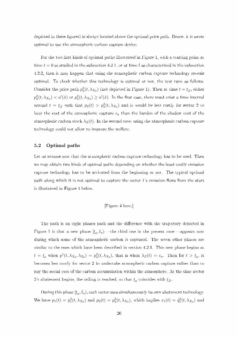
5.2 Optimal paths

Let us assume now that the atmospheric carbon capture technology has to be used. Then

we may obtain two kinds of optimal paths depending on whether the least costly emission

capture technology has to be activated from the beginning or not. The typical optimal

path along which it is not optimal to capture the sector 1's emission �ows from the start

is illustrated in Figure 4 below.

[Figure 4 here.]

The path is an eight phases path and the di�erence with the trajectory depicted in

Figure 1 is that a new phase [ta, ta) � the third one in the present case � appears now

during which some of the atmospheric carbon is captured. The seven other phases are

similar to the ones which have been described in section 4.2.1. This new phase begins at

t = ta when p1(t, λX0 , λZ0) = p2a(t, λX0), that is when λZ(t) = ca. Then for t > ta, it

becomes less costly for sector 2 to undertake atmospheric carbon capture rather than to

pay the social cost of the carbon accumulation within the atmosphere. At the time sector

2's abatement begins, the ceiling is reached, so that ta coincides with tZ .

During this phase [ta, ta), each sector uses simultaneously its own abatement technology.

We have p1(t) = p2e(t, λX0) and p2(t) = p2

a(t, λX0), which implies x1(t) = q2e(t, λX0) and

20

x2(t) = q2a(t, λX0). Since ce < ca, we also have p1(t) < p2(t) and then x1(t) > x2(t).

Remember that, during this phase, as in the phase 3 of subsection 4.2.1, sector 1's emissions

are fully captured: se(t) = ζx1(t). Because this is a phase at the ceiling, sector 2 has just

to capture in the atmosphere the necessary amount of carbon in order to maintain the

atmospheric carbon stock at its critical level. It is thus optimal for sector 2 to abate at

a level which is smaller than its own carbon emissions: sa(t) = ζx2(t) − αZ < ζx2(t).

Moreover, since sa(t) > 0, we have ζx2(t) > αZ, or equivalently, x2(t) > x, implying in

turns p2(t) < u′(x). The price path p2(t) = p2a(t, λX0) being increasing through time, �rst

the amount of abated carbon by the atmospheric device sa(t) is decreasing, second there

must exist a date at which p2(t) = u′(x), that is at which x2(t) = x and sa(t) = 0. At that

time, denoted by ta, since sector 1 still fully abates all its emissions, it is no more optimal

for sector 2 to pursue the atmospheric carbon capture. All the e�orts to maintain the

carbon stabilization cap are now supported by the sole sector 1 and the economy behaves

as in section 4.2.1 from phase 3, that if from the date tZ as depicted in Figure 1.

To the eight variables parameterizing the optimal path in the case without atmospheric

capture technology (cf. subsection 4.2.1), we must here determine the values of two ad-

ditional variables: ta and ta. But because ta = tZ , then only one more variable has to

be determined. Hence we are left with nine variables that must solve the following nine

equations system:

- Balance equation of non-renewable resource consumption and supply:

2∫ te

0q1(t, λX0 , λZ0)dt+

∫ ta=tZ

te

[q1(t, λX0 , λZ0) + q2

e(t, λX0)]dt

+∫ ta

ta=tZ

[q2e(t, λX0) + q2

a(t, λX0)]dt+

∫ t

ta

[q2e(t, λX0) + x

]dt

+2∫ te

tq2e(t, λX0)dt+ [tZ − te] x+ 2

∫ ty

tZ

q3(t, λX0)dt = X0. (50)

- Continuity of the carbon stock at time tZ : identical to (40).

- Price continuity equations: identical to (41)-(46) except that (42) is now replaced by

the two following equations:

p1 (ta, λX0 , λZ0) = p2a(ta, λX0) (51)

p2a (ta, λX0) = u′(x) (52)

21

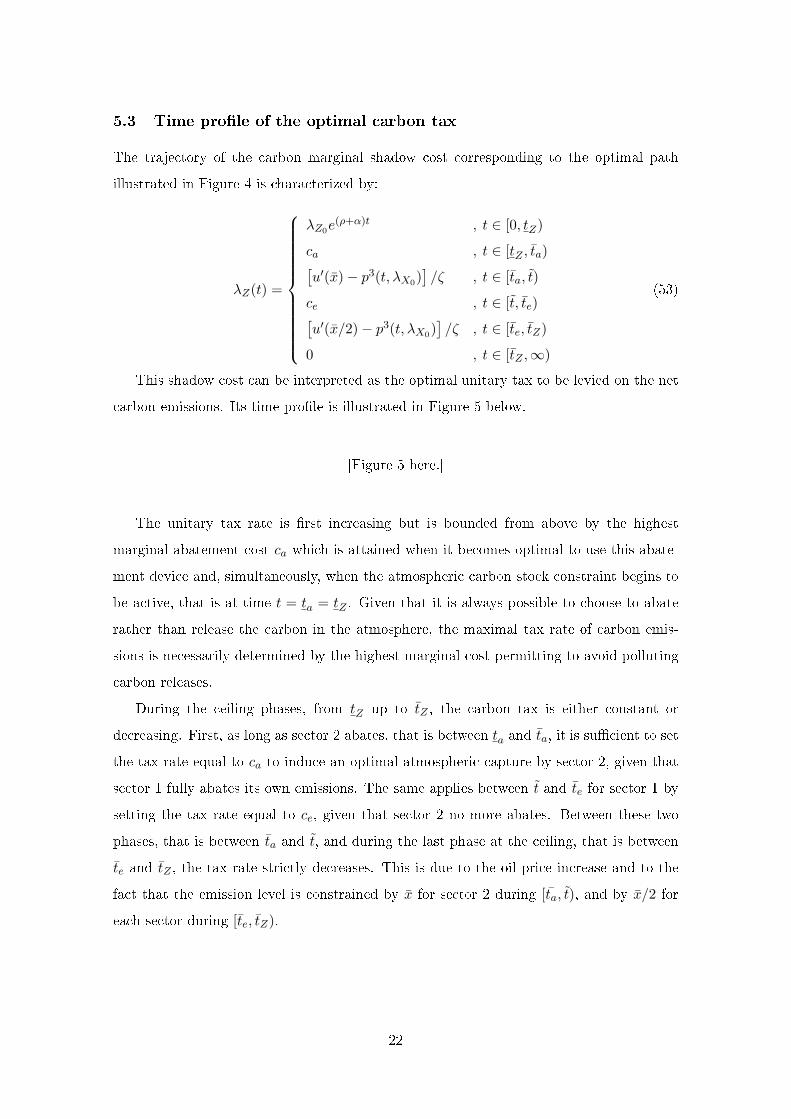
5.3 Time pro�le of the optimal carbon tax

The trajectory of the carbon marginal shadow cost corresponding to the optimal path

illustrated in Figure 4 is characterized by:

λZ(t) =

λZ0e(ρ+α)t , t ∈ [0, tZ)

ca , t ∈ [tZ , ta)[u′(x)− p3(t, λX0)

]/ζ , t ∈ [ta, t)

ce , t ∈ [t, te)[u′(x/2)− p3(t, λX0)

]/ζ , t ∈ [te, tZ)

0 , t ∈ [tZ ,∞)

(53)

This shadow cost can be interpreted as the optimal unitary tax to be levied on the net

carbon emissions. Its time pro�le is illustrated in Figure 5 below.

[Figure 5 here.]

The unitary tax rate is �rst increasing but is bounded from above by the highest

marginal abatement cost ca which is attained when it becomes optimal to use this abate-

ment device and, simultaneously, when the atmospheric carbon stock constraint begins to

be active, that is at time t = ta = tZ . Given that it is always possible to choose to abate

rather than release the carbon in the atmosphere, the maximal tax rate of carbon emis-

sions is necessarily determined by the highest marginal cost permitting to avoid polluting

carbon releases.

During the ceiling phases, from tZ up to tZ , the carbon tax is either constant or

decreasing. First, as long as sector 2 abates, that is between ta and ta, it is su�cient to set

the tax rate equal to ca to induce an optimal atmospheric capture by sector 2, given that

sector 1 fully abates its own emissions. The same applies between t and te for sector 1 by

setting the tax rate equal to ce, given that sector 2 no more abates. Between these two

phases, that is between ta and t, and during the last phase at the ceiling, that is between

te and tZ , the tax rate strictly decreases. This is due to the oil price increase and to the

fact that the emission level is constrained by x for sector 2 during [ta, t), and by x/2 for

each sector during [te, tZ).

22

5.4 Time pro�le of the tax burdens and the sequestration costs

Assume now that the above tax optimal rate is implemented. Such a tax is inducing a

�scal income Γ1(t) ≡ [ζx1(t)− se(t)]λZ(t) for sector 1 and Γ2(t) ≡ [ζx2(t)− sa(t)]λZ(t) for

sector 2. The sequestration cost in each sector simply writes as the sequestered carbon �ow

times the respective marginal cost of sequestration: S1(t) ≡ se(t)ce and S2(t) ≡ sa(t)ca.

Then, the total burden of carbon for each sector is the sum of the �scal burden and the

sequestration cost. Denoting by Bi(t) i = 1, 2 this total burden, the two following tables

details its components for each sector.

Γ1(t) S1(t) B1(t) Phases

ζq1(t)λZ0e(ρ+α)t 0 ζq1(t)λZ0e

(ρ+α)t [0, te)

0 ζq2e(t)ce ζq2

e(t)ce [te, t)

ζ[x− q2

e(t)]ce ζ

[2q2e(t)− x

]ce ζq2

e(t)ce [t, te)

(x/2)[u′(x/2)− p3(t)

]0 (x/2)

[u′(x/2)− p3(t)

][te, tZ)

0 0 0 [tZ ,∞)

Table 1. Decomposition of the total carbon burden in sector 1.

Γ2(t) S2(t) B2(t) Phases

ζq1(t)λZ0e(ρ+α)t 0 ζq1(t)λZ0e

(ρ+α)t [0, ta)

ζxca ζ[q2a(t)− x]ca ζq2

a(t)ca [ta, ta)

x[u′(x)− p3(t)

]0 x

[u′(x)− p3(t)

][ta, t)

ζq2e(t)ce 0 ζq2

e(t)ce [t, te)

(x/2)[u′(x/2)− p3(t)

]0 (x/2)

[u′(x/2)− p3(t)

][te, tZ)

0 0 0 [tZ ,∞)

Table 2. Decomposition of the total carbon burden in sector 2.

Their time pro�le are depicted by Figure 6 below.

23

[Figure 6 here.]

Before the ceiling phases, the shapes of the total burden trajectories may be either

increasing or decreasing depending upon oil demand elasticity. Once the ceiling is reached,

the total burden gradually declines down to zero at the end of the ceiling phase.

For sector 1, the total burden identi�es to the sole tax burden as long as abatement is

not activated, that is before te. Between te and t, sector 1, fully abating its emissions, does

not bear the carbon tax burden (Γ1(t) = 0), but bears the sequestration cost S1(t). During

this phase, since sector 1's emissions decrease, so does its sequestration cost and then its

total burden. During the next phase, between t and te, it is no more optimal for sector 1

to fully abate its emissions and then, this sector bears a mix of tax burden and abatement

cost. Its gross carbon emissions decrease, but its sequestration �ow decreases at an even

higher rate resulting in an increase in the net emission �ow. The cost of sequestration thus

decreases. Since the tax rate is constant and equal to the sequestration marginal cost ce,

the �scal burden rises. The combined e�ect of these two evolutions results in a declining

total carbon burden for sector 1. Over the last ceiling phase, between te and tZ , sector 1

no more abates and bears only the �scal burden. Then its total burden is declining down

to zero when the ceiling constraint becomes no more active, that is at time tZ .

Sector 2 bears simultaneously the tax and the sequestration cost burden only during the

atmospheric capture phase, that is between ta and ta. During this phase, its �scal burden

is constant because i) the tax rate is constant and equal to ca and ii) sector 1 fully abates

its emissions and sector 2's net emissions are constrained by x. Its sequestration e�ort

decreases since gross emissions decline. After ta and during all next phases at the ceiling,

the total burden of sector 2 reduces to the sole �scal burden and it is thus decreasing over

time as discussed above.

We conclude by two remarks. First, the total �scal income, that is Γ1(t) + Γ2(t),

jumps down twice at each time where either sector 1 or sector 2 begins to abate. Then,

any environmental policy should take into account the ability of polluters to undertake

abatement activities and thus to escape from the tax. Second, since sector 2 is constrained

by the higher cost of its abatement technology, its �scal contribution as well as its total

burden are larger or equal than the total burden of sector 1 when pollutive potential

intensities and demand functions are the same for both sectors.

24

6 Conclusion

In a Hotelling depletion model, we have determined the optimal exploitation time paths of

two energy resources, one being depletable and carbon-emitting, the other being renewable

and carbon-free, by two sectors that are heterogeneous regarding their respective abatement

capacities. The optimal paths have been considered along with the following features.

First, sector 1 is able to abate its carbon emissions, but not sector 2. Second, to reduce

pollution, sector 2 can only have recourse to the atmospheric capture technology, which

is highly more expensive than the emission capture. Third, the cumulative atmospheric

carbon stock is set not to exceed some critical threshold.

We have shown that the optimal path requires that emission abatement by sector 1

must be undertaken before the point of time at which the atmospheric carbon stock reaches

its critical threshold and that sector 1's emissions must be wholly abated. This �rst result

contrasts with the results established by Chakravorty el al. (2006-b) in a model with a

single energy using sector and a single abatement technology. It can thus be explained

by the assumption of heterogeneity introduced here, which constraints the potential of

emission capture to be at the most equal to the sole emissions of sector 1 and then to be

always smaller the total carbon emissions of fossil energy users.

Heterogeneity means that the abatement costs are not the same for all the energy

users. This is the crucial assumption generating the early and full abatement of sector 1's

potential emissions. Clearly in the present model we could have assumed that the sector

2 can abate its emissions at the marginal cost ca instead of having to capture the carbon

in the atmosphere. The reason is that the �ow of carbon captured in the atmosphere

is lower than the potential carbon emission �ow of sector 2 when carbon is captured in

the atmosphere. Thus would the carbon be captured from sector 2's emissions at the

marginal cost ca the result would be the same, that is the optimal price paths, optimal

sectoral consumption paths and captured carbon paths by the two abatement technologies

would be the same. To reinforce the heterogeneity argument, we show in a companion

paper (Amigues et al., 2010) that, when all the energy consumers have access to the same

abatement costs, then even learning by doing in the abatement technology does not justify

to begin to abate too early, that is before being at the ceiling10.

Last, remark that atmospheric carbon capture by sector 2 is implemented only once

10However, note that the time at which Z(t) reaches its critical level Z is endogenous. Thus learning bydoing is not without e�ect on this date.

25

the ceiling is reached and sector 2's intensity of abatement is always smaller than its real

contribution to the common atmospheric carbon accumulation, which is now in accordance

with the results of Chakravorty et al. (2006-b).

26

References

[1] Amigues, J.P., La�orgue, G. and Moreaux, M. (2010). Optimal abatement policies

of potential carbon emissions with learning by doing in abatement. LERNA working

paper, Toulouse School of Economics.

[2] Barrett, S. (2009). Climate treaties with a backstop technology. Working Paper,

Columbia University.

[3] Chakravorty, U., Magné, B. and Moreaux, M. (2006-a). Plafond de concentration

en carbone et substitutions entre ressources énergétiques. Annales d'Economie et de

Statistiques, 81, 141-168.

[4] Chakravorty, U., Magné, B. and Moreaux, M. (2006-b). A Hotelling model with a

ceiling on the stock of pollution. Journal of Economic Dynamics and Control, 30,

2875-2904.

[5] Edmonds, J., Clarke, J., Dooley, J., Kim, S.H., Smith, S.J. (2004). Stabilization of

CO2 in a B2 world: insights on the roles of carbon capture and disposal, hydrogen,

and transportation technologies. Energy Economics, 26, 517-537.

[6] Gerlagh, R., van der Zwaan, B.C. (2006). Options and instruments for a deep Cut in

CO2 emissions: carbon capture or renewable, taxes or subsidies? Energy Journal, 27,

25-48.

[7] Intergovernmental Panel on Climate Change (2005). Special Report on Carbon Diox-

ide Capture and Storage, Working Group III.

[8] Intergovernmental Panel on Climate Change (2007). Climate Change 2007, Synthesis

Assessment Report, Working Group III.

[9] Islegen, O., Reichelstein, S. (2009). The economics of carbon capture. The Economist's

Voice, December: The Berkeley Electronic Press.

[10] La�orgue, G., Magne B., Moreaux M. (2008-a). Energy substitutions, climate change

and carbon sinks. Ecological Economics, 67, 589-597.

[11] La�orgue, G., Magne B., Moreaux M. (2008-b). The optimal sequestration policy with

a ceiling on the stock of carbon in the atmosphere. In The Design of Climate Policy

(Chapter 14, pp. 273-304), R. Guesnerie and H. Tulkens eds, Boston: The MIT Press.

27

[12] McFarland, J.R., Herzog, H.J., Reilly, J.M., 2003. Economic modelling of the global

adoption of carbon capture and sequestration technologies. In: Proceedings of the Sixth

International Conference on Greenhouse Gas Control Technologies, Gale, J., Kaya, Y.

(Eds.). Elsevier Science, Oxford.

[13] McKay, D. (2009). Sustainable energy - Without the hot air. UIT Cambridge Ltd.:

Cambridge.

[14] McKinsey & Company (2007). Reducing U.S. greenhouse gas emissions: How much

at what cost? Available at:

http://www.mckinsey.com/clientservice/ccsi/greenhousegas.asp.

[15] MIT (2007). The future of coal. Available at: http://web.mit.edu/coal.

28

0t

yc

( )tp

0Xxc λ+

00 ZXxc ζλλ ++

eXx cc ζλ ++0

( )2/xu′

( )xu′

( )0

,3Xtp λ

et t etZt t~ Zt yt

( )0

,2Xe tp λ( )

00,,1

ZXtp λλ

21 pp =

21 pp =

21 pp =

21 pp =

21 pp =

1p

1p2p

2p

Zζλ

Zζλ

Period at the ceiling

Full capture of sector 1’s emissions

Partial capture of sector 1’s emissions

Figure 1: Optimal path along which it is optimal to abate before the ceiling, but not fromthe beginning of the planning horizon

29

0t

yc

( )tp

0Xxc λ+

00 ZXxc ζλλ ++

eXx cc ζλ ++0

( )2/xu′

( )xu′

( )0

,3Xtp λ

etZe tt = Zt yt

( )0

,2Xe tp λ( )

00,,1

ZXtp λλ

Period at the ceiling

Full capture of sector 1’s emissions

eZ cζζλ =

Figure 2: Optimal path along which the energy price is the same for each sector and it isoptimal to abate sector 1's emissions

30

0t

yc

( )tp

0Xxc λ+

00 ZXxc ζλλ ++

eXx cc ζλ ++0

( )2/xu′

( )0

,3Xtp λ

Zt Zt yt

( )0

,2Xe tp λ( )

00,,1

ZXtp λλ

Period at the ceiling

Figure 3: Optimal path along which the energy price is the same for each sector and it isnot optimal to abate sector 1's emissions

31

0t

yc

( )tp

0Xxc λ+00 ZXxc ζλλ ++

eXx cc ζλ ++0

( )2/xu′

( )xu′

( )0

,3Xtp λ

et etaZ tt = t~ Zt yt

( )0

,2Xe tp λ( )

00,,1

ZXtp λλ

21 pp =

21 pp =21 pp = 21 pp =

1p1p

2p

2p

Period at the ceiling

Full capture of sector 1’s emissions

Partial capture of sector 1’s emissions

( )0

,2Xa tp λ

aXx cc ζλ ++0

at

2p

1p

Atmospheric capture

Figure 4: Optimal path requiring to activate the both carbon capture devices

32

0t

( )tZλ

ec

et etaZ tt = t~ Ztat

tZ e )(

0

αρλ +

ac

0Zλ

Figure 5: Time pro�le of the optimal unitary carbon tax

0t

et etaZ tt = t~ Ztat

acxζ

21 BB =

1B

2B

2Γ

2S

2B

21 BB =

21 BB =

1B

1S

1Γ

1S

ecxζ

ecx2

ζ

Figure 6: Total burden of carbon for each sector

33