MASSACHUSETTS INSTITUTE OF TECHNOLOGY

2.71/2.710 Optics Spring ’14 Practice Problems for the Final Exam Posted Monday, May 17, 2014

1. (Pedrotti 13-21) A glass plate is sprayed with uniform opaque particles. When a distant point source of light is observed looking through the plate, a diffuse halo is seen whose angular width is about ቄኲ . Estimate the size of the particles. (Hint: consider Fraunhoffer diffraction through random gratings, and use Babinet’s principle)

Answer: The diffraction pattern of an opaque circular particle is complementary to that due to circular apertures of the same size in an otherwise opaque screen.

ኮሐኻዂዾሎኼዂ

ዾሑ ኮሻኻዾሎኼዾሿ

Under the Fraunhofer condition ( ዷ ቃ, ዷ ቃ)ሆኽ ሆኽ

ቃ ዷሊሤ ሥላ ሞ ኅቪቢሊሖሕሗሊኰኻዂሤ ሕ ኰኼዂሥላላሠሊሤ ሥላዷሊሤ ሥላሐሤሐሥ

ሦ ኻ ኼ

Where ኰኻዂ ሞ , ኰኼዂ ሞ ኽ ኽ

For the given problem, we may further assume E(x, y) is a plane wave at normal incidence, and the transmission function t(x, y) for a single can be expressed as:

ትሤሆ ሕ ሥሆ

ሠሊሤ ሥላ ሜ ቃ ሖ ሏሕሞሏሊ ላ ሄ

Where ሄ is the radius of the opaque particles.

ቃ ትሤሆ ሕ ሥሆ

ዷሊሤ ሥላ ሞ ኅቪቢሊሖሕሗሊኰኻዂሤ ሕ ኰኼዂሥላላ ስቃ ሖ ሏሕሞሏሊ ላሹ ሐሤሐሥ ሦ ሄ

ቃ ትሤሆ ሕ ሥሆ

ዷሊሤ ሥላ ሞ ኰ ስቃ ሖ ሏሕሞሏ ሽ ቁሹ ሦ ሄ

ኽ ኽWith ሤ ሜ ሗኻ , ሥ

ሜ ሗኼኮ ኮ

ኝ ቄኸዼቃ ሖሄቷሗሤቄ ሕ ሗሥ

ቄሗአ ቃ ኞ ኡ

ዷሻሗኻ ሗኼሿ ሞ ኬሊቷሗሤቄ ሕ ሗሥ

ቄላ ሖ ዑሄዑቄ ኞ ኡ ሦ ቄ ቄኞ ሄቷሗሤ ሕ ሗሥ ኡ ኟ ኢ

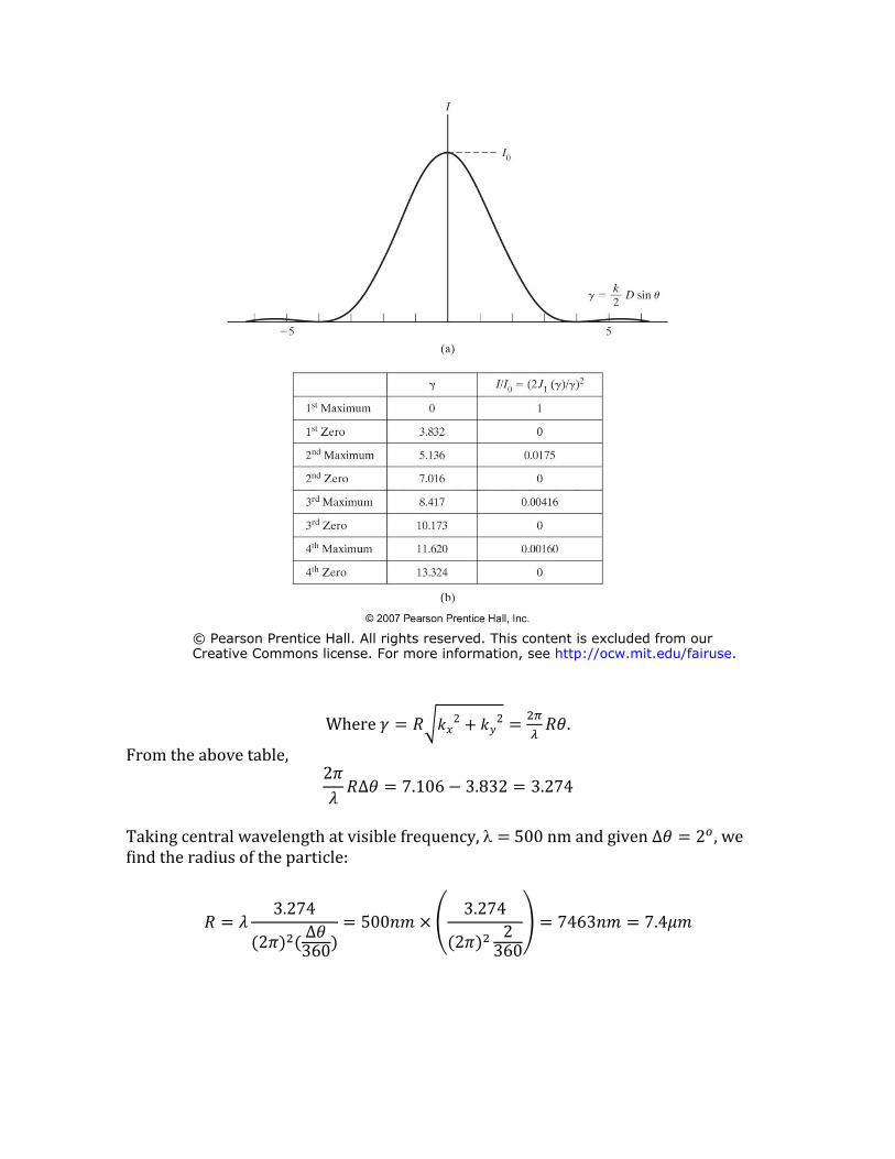
The halo is similar to an Airy disc! We can evaluate the width of the halo (a second peak) based on the table on Figure 11_08 provided by Pedrotti:

ቄ ሜ ሆዧ

Where ካ ሜ ሄቷሗሤቄ ሕ ሗሥ ሄኰ.

ዢ

From the above table, ቄኸ

ሄኰ ሜ ኴቃቂቈ ሖ ቅኴቊቅቄ ሜ ቅኴቄቆ ኳ

Taking central wavelength at visible frequency, = 500 nm and given ኰ ሜ ቄኲwe find the radius of the particle:

ቅኴቄቆ ቅኴቄቆ ሄ ሜ ኳ ሜ ቇቂቂሚሙ መ ሜ ቍ ሜ ቆቈቅሚሙ ሜ ኴቆኴሙ

ኰ ቄ ሊቄኸላሆሊ ላ ሊቄኸላሆ

ቅቈቂ ቅቈቂ

© Pearson Prentice Hall. All rights reserved. This content is excluded from ourCreative Commons license. For more information, see http://ocw.mit.edu/fairuse.

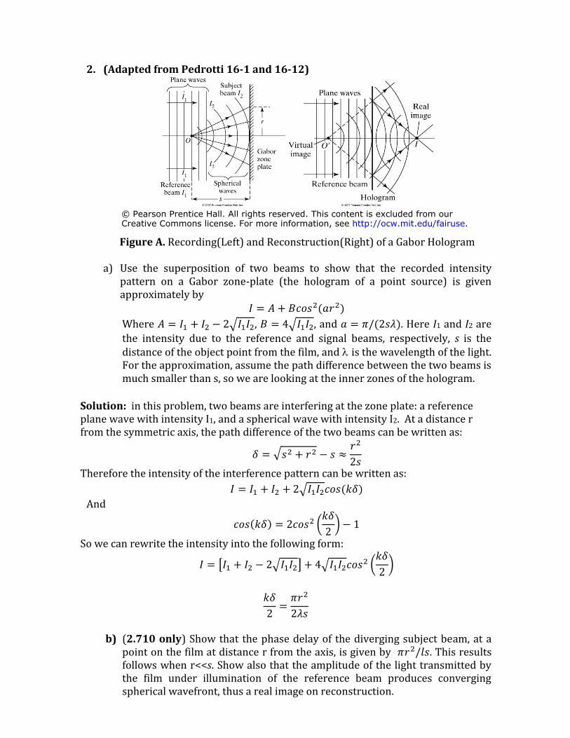
2. (Adapted from Pedrotti 16-1 and 16-12)

Figure A. Recording(Left) and Reconstruction(Right) of a Gabor Hologram

a) Use the superposition of two beams to show that the recorded intensity pattern on a Gabor zone-plate (the hologram of a point source) is given approximately by

ዻ ሜ ዳ ሕ ዴሏማሟሆሊልሞሆላ

Where ዳ ሜ ዻህ ሕ ዻሆ ሖ ቄትዻህዻሆ, ዴ ሜ ቆትዻህዻሆ, and ል ሜ ኸዐሊቄሟኳላ. Here I1 and I2 are

the intensity due to the reference and signal beams, respectively, s is the distance of the object point from the film, and is the wavelength of the light. For the approximation, assume the path difference between the two beams is much smaller than s, so we are looking at the inner zones of the hologram.

Solution: in this problem, two beams are interfering at the zone plate: a reference plane wave with intensity I1, and a spherical wave with intensity I2. At a distance r from the symmetric axis, the path difference of the two beams can be written as:

ሞሆ

ኬ ሜ ትሟሆ ሕ ሞሆ ሖ ሟ ሞ ቄሟ

Therefore the intensity of the interference pattern can be written as:

ዻ ሜ ዻህ ሕ ዻሆ ሕ ቄትዻህዻሆሏማሟሊሗኬላ And

ሗኬ ሏማሟሊሗኬላ ሜ ቄሏማሟሆ ሼ ቀ ሖ ቃ

ቄ So we can rewrite the intensity into the following form:

ሗኬ ዻ ሜ ሳዻህ ሕ ዻሆ ሖ ቄትዻህዻሆሷ ሕ ቆትዻህዻሆሏማሟ

ሆ ሼ ቀ ቄ

ሗኬ ኸሞሆ

ሜ ቄ ቄኳሟ

b) (2.710 only) Show that the phase delay of the diverging subject beam, at a point on the film at distance r from the axis, is given by ኸሞሆዐመሟ. This results follows when r<<s. Show also that the amplitude of the light transmitted by the film under illumination of the reference beam produces converging spherical wavefront, thus a real image on reconstruction.

© Pearson Prentice Hall. All rights reserved. This content is excluded from ourCreative Commons license. For more information, see http://ocw.mit.edu/fairuse.

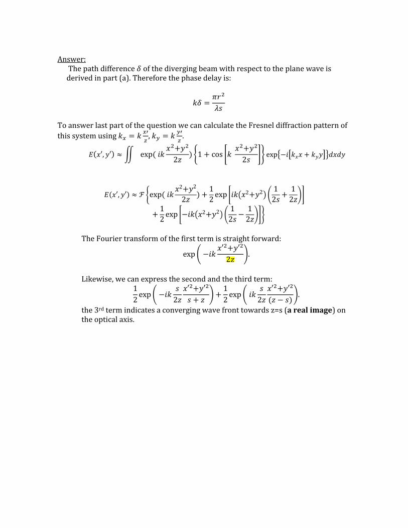
Answer: The path difference ኬ of the diverging beam with respect to the plane wave is derived in part (a). Therefore the phase delay is:

ኸሞሆ

ሗኬ ሜ ኳሟ

To answer last part of the question we can calculate the Fresnel diffraction pattern of ኻ ኼ

this system using ሗኻ ሜ ሗ , ሗኼ ሜ ሗ . ኽ ኽ

ሤሆሕሥሆ ሤሆሕሥሆ

ዷሊሤዲ ሥዲላ ሞ ኅ ቪቢሊሕሗ ላ ሚቃ ሕ ቕቡብመሗ ሙማ ቪቢራሖሕሳሗሤሤ ሕ ሗሥሥሷሯሐሤሐሥ ቄሦ ቄሟ

ሤቄሕሥቄ ቃ ቃ ቃ ዷሊሤዲ ሥዲላ ሞ ኰ ሚቪቢሊሕሗ ላ ሕ ቪቢ መሕሗሻሤቄሕሥቄሿ ሖ ሕ ሗሙ

ቄሦ ቄ ቄሟ ቄሦ ቃ ቃ ቃ

ሕ ቪቢ መሖሕሗሻሤቄሕሥቄሿ ሖ ሖ ሗሙማ ቄ ቄሟ ቄሦ

The Fourier transform of the first term is straight forward: ሤዲሆሕሥዲሆ

ቪቢ ሖሖሕሗ ሗኴ ቄሦ

Likewise, we can express the second and the third term: ቃ ሟ ሤዲሆሕሥዲሆ ቃ ሟ ሤዲሆሕሥዲሆ

ቪቢ ሖሖሕሗ ሗ ሕ ቪቢ ሖሕሗ ሗኴ ቄ ቄሦ ሟ ሕ ሦ ቄ ቄሦ ሊሦ ሖ ሟላ

the 3rd term indicates a converging wave front towards z=s (a real image) on the optical axis.

4. Consider the optical system shown the following schematic, where lenses L1, L2

are identical with focal length f and diameter 2a. A thin-transparency object T1 is

placed at distance 2f to the left of L1.

a) Where is the image formed? Use geometrical optics, ignoring the lens

apertures for the moment.

From the lens formula, we can calculate the location of the image after L1 and L2 as:

1

1

2 1

2

2

,1 1 1

2

1 1

2

3

1,

i

i

o i

i

i

s f

s f

f s f

s f

fs

s f

Therefore, the image is located at infinity, to the right of L2.

b) If the object T1 is an on-axis point source, describe the Fraunhofer diffraction

pattern of the field to the right of L2.

The object T1 is imaged to the front focal plane of L2, and therefore is turned into a plane

wave after passing through L2. The Fraunhofer diffraction pattern a uniform plane wave.

c) How are your two previous answers consistent within the approximations of

paraxial geometrical and wave optics?

Answer for (a) obtained with geometrical ray optics matches the answer from (b), which is

obtained from wave optics calculation under the paraxial approximation. Both predicts that

the image after L2 will propagate straight to infinity, in the form of a plane wave.

d) The point source object T1 is replaced by a clear aperture of full width w and a

second thin transparency T2 is placed between the two lenses, at distance f to

11 1) ( )( 1

xT rectx

W

2

2 2

2

2 )e e

( ) ( exp 2 ]exp[[ ]

jkjkf

L f L f

X

f X xE X E dx

j fx j x jk

ff

the left of L2. The system is illuminated coherently with a monochromatic on-

axis plane wave at wavelength λ. Write an expression for the field at distance

2f to the right of L2 and interpret the expression that you found.

A monochromatic on-axis plane wave hits the aperture of full width w at T1. This plane

wave focuses into a point at the focal plane of L1, and is imaged as a point at a distance 2f

away from L2. With no waveplates, a plane wave focuses into a point, at a distance 2f to the

right of L2.

Let us now consider the effect of transparencies. The 2D problem in (x,z) is calculated. The

field on the T1 plane can be expressed as:

.

The plane wave focuses at the distance f to the right of L1.

Since T2 is located exactly at the image plane of T1, the image of T1 is multiplied to the

transparency T2.

22 2 2 2'( ( ) ( )) T

x

WT x rect x

Effectively, this modified transparency is illuminated with a point source located 2f to the

left of L2. At the plane of T2, this illumination can be expressed as:

22

22

2

2

2 22 2 2 2 2 2

( )

( ) ' ( )T

1

1( ) ( ) ( )

xjk

jkf f

xjk

jkf f

E e ef

E E e e rect xf

xj

xx x T x

j W

Because T2 is located at the focus of L2, the Fourier transform of is located at the

distance f to the right of L2. 2TE

2

2

2exp[( ) sinc(] )FT{T }|jkf

L f x

f

e xE

Wx j f j x

jW

ff

f

At the distance 2f to the right of L2, this field is Fresnel propagated for an additional

distance f, so the analytical expression can be written as:

.

Qualitatively, this image resembles a point, if T2 does not produce additional spatial

frequency components.

2 22 / 2 /22 2 ) [1 cos ]

21 1 1 1(

2 2 4 4

i x xixx e eT

22

2 22 / 2 /2 22

1 1 1( ) ( )

4

1

2 4

xjk

i ijkf f x xE e e rect

f

xx e e

j W

2

3 3

2

2

2

3 3

2

2

2

2

3/2 3/2

e e( ) ...

...e

1 12 ( ) sinc( )e ( ) ( )

4

2 ]exxp[ ]

e

p[

sinc(e

2 ] exp[ exp)e exp[ 2 2 [] ]4

2

X

f j

jkfjkf jkf

L f

jkfjkf

X

f j

e x W x xE X

j f f f f

X xdx

f

W

f

j x

W f

jkf

j jX X

jj

f

2 3 3

22

e since 1 sin( )( ) 2

fjk j

X fj

fCW X

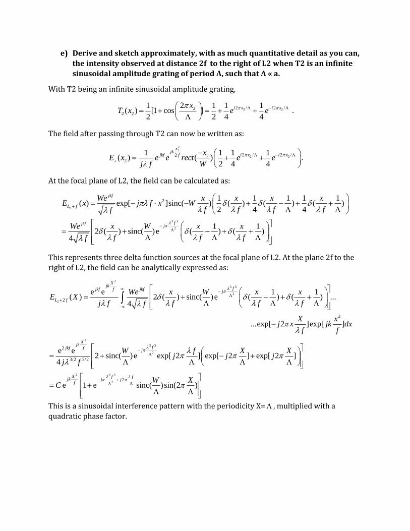
e) Derive and sketch approximately, with as much quantitative detail as you can,

the intensity observed at distance 2f to the right of L2 when T2 is an infinite

sinusoidal amplitude grating of period Λ, such that Λ « a.

With T2 being an infinite sinusoidal amplitude grating,

.

The field after passing through T2 can now be written as:

.

At the focal plane of L2, the field can be calculated as:

2

3 3

2

2 1 1 1 1 1exp[ ] ) ( ) ( ) ( )

2 4 4

1 12 ( ) sinc( )e ( ) ( )

( ) sinc(

4

jkf

L f

fjkf j

e x x x xE W

f f f f

e x W x x

Wx j f x

f

W

f f f f

This represents three delta function sources at the focal plane of L2. At the plane 2f to the

right of L2, the field can be analytically expressed as:

This is a sinusoidal interference pattern with the periodicity X= , multiplied with a

quadratic phase factor.

general formulations for the 4–

� �

� � � �

MASSACHUSETTS INSTITUTE OF TECHNOLOGY

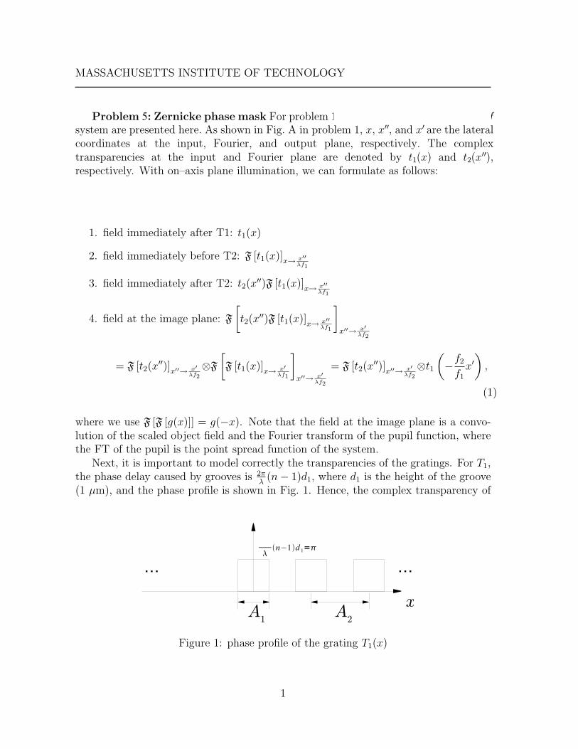
Problem 5: Zernicke phase mask For problem 1, f system are presented here. As shown in Fig. A in problem 1, x, x"" , and x" are the lateral coordinates at the input, Fourier, and output plane, respectively. The complex transparencies at the input and Fourier plane are denoted by t1(x) and t2(x"" ), respectively. With on–axis plane illumination, we can formulate as follows:

1. field immediately after T1: t1(x)

2. field immediately before T2: F [t1(x)]x→ ''x

λf1

3. field immediately after T2: t2(x"" )F [t1(x)]x→ ''x

λf1

4. field at the image plane: F t2(x"" )F [t1(x)]x→ ''x

'λf1 ''→ xx λf2

f2 " = F [t2(x "" )]x''→ x' ⊗F F [t1(x)]x→ x' = F [t2(x "" )]x''→ x' ⊗t1 − x , 'λf2 λf1 ''→ x λf2 f1x λf2

(1)

where we use F [F [g(x)]] = g(−x). Note that the field at the image plane is a convo­lution of the scaled object field and the Fourier transform of the pupil function, where the FT of the pupil is the point spread function of the system.

Next, it is important to model correctly the transparencies of the gratings. For T1, the phase delay caused by grooves is 2

λπ (n − 1)d1, where d1 is the height of the groove

(1 µm), and the phase profile is shown in Fig. 1. Hence, the complex transparency of

Figure 1: phase profile of the grating T1(x)

1

� � � �

� �

� �

�

�����

�����

�����

T1 is written as �

2π x x ���

iφ1(x)t1(x) = e = exp i (n − 1)d1 rect ⊗ comb , (2)λ A1 A2

where A1 = 5 µm and A2 = 10 µm. Hence, �

eiπ(= −1) if |x| < A1/2,t1(x) = (3)1 if A1/2 < x < A2/2 or − A2/2 < x < −A1/2,

for |x| < A2/2. Using the Fourier series (C t1(x) is periodic) and A = A2 = 2A1, we find the Fourier series coefficients as

� A/21 2π−i A qxdxcq = t1(x)e A −A/2 �� −A/41 2π−i A

� A/4 � A/2

e 2π−i A qxdx + A−i 2π

eqxdx − qxdx (4)= e

A

A −A/2 −A/4 A/4

1For q = 0, c0 = A

J t1(x)dx = 0.

For q = 0,

A

⎡ −A/4 A/4 A/2

⎤−i 2π −i 2π −i 2π

A qx qx qx1 e e e⎣ ⎦− +c = q −i2π A −i2π

A −i2π A

A q q q−A/2 −A/4 A/4

i π −i π i π −i πiπq q q1 e 2 q − e e 2 q − e 2 e−iπq − e 2

= − + A −i2π q −i2π q −i2π qA A A

−iπq i π −i π qeiπq − e e 2 q − e 2 �q� �q�

= − = sinc (q) − sinc = −sinc . i2πq i2π

2 q 2 2

Thus, cq = −sinc (

2 q )

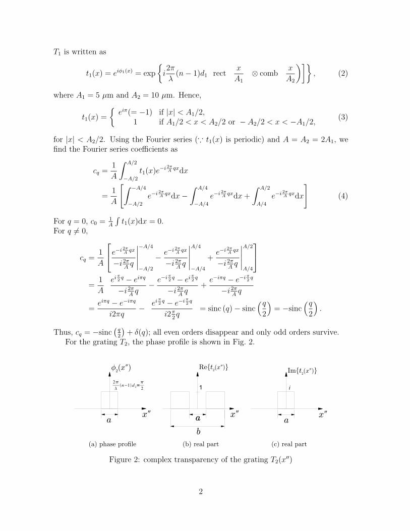
+ δ(q); all even orders disappear and only odd orders survive. For the grating T2, the phase profile is shown in Fig. 2.

(a) phase profile (b) real part (c) real part

"" )Figure 2: complex transparency of the grating T2(x

2

� � � � � �

� �

� � � �

� � � � � �

� � � � � � � �

� � � � � � � �

� � � �

Figure 3: the field immediately before T2.

The complex transparency can be written as "" "" "" x x

�� x

t2(x "" ) = rect − rect + irect . (5)b a a

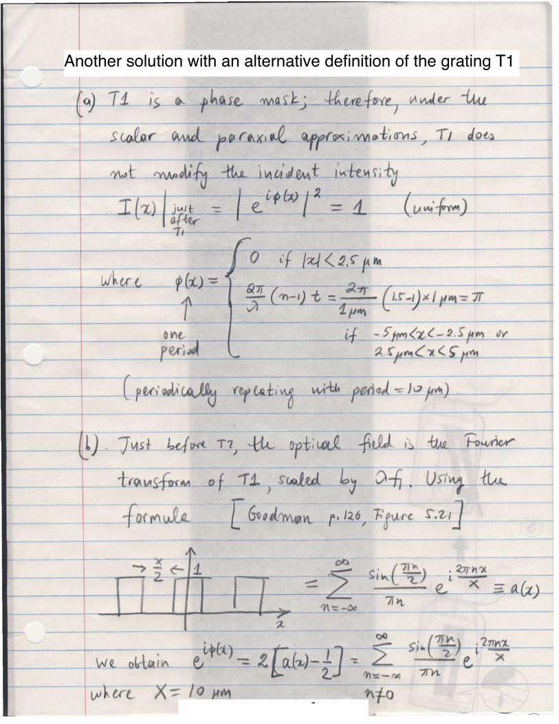
a) the intensity immediately after T1 is 1 because |t1(x)|2 = 1. Since T1 is a pure phase object and there is no intensity variation.

b) the field immediately before T2 can be computed from the Fourier series co­efficients of t1(x). Since the period of T1 is A, the diffraction angle of the order q is

= q λ , and the diffraction order q is focused at f1θq on the Fourier plane. Hence, the θq A field immediately before T2 is

∞ ∞f1λ"" ""

� (δ(q) − sinc (q/2)) δ x − q =

� (δ(q) − sinc (q/2)) δ (x − q cm) . (6)

A q=−∞ q=−∞

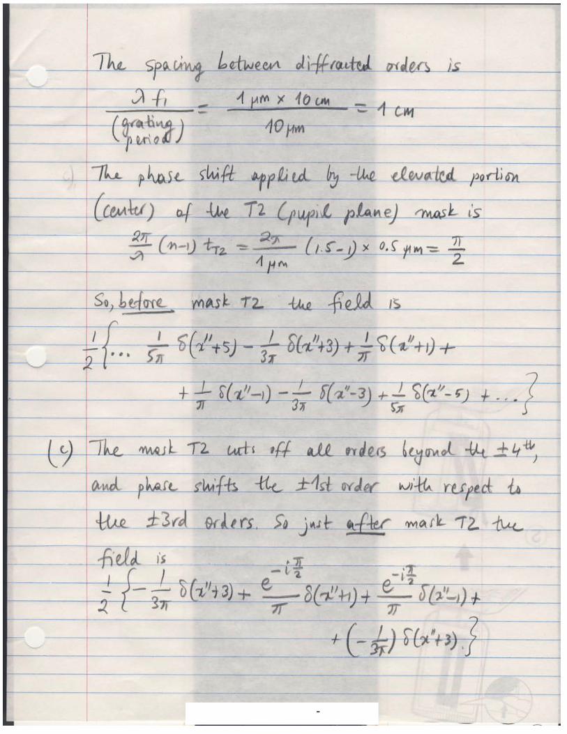
c) Since b (the width of the grating T2) is 7 cm, the diffraction orders passing through the grating T2 are q = −3, −1, +1, +3, where −1 and +1 orders get phase delay of π/2. The field immediately after the grating is

3 i π 1"" "" "" "" −sinc [δ(x − 3) + δ(x + 3)] − e 2 sinc [δ(x − 1) + δ(x + 1)] . (7)2 2

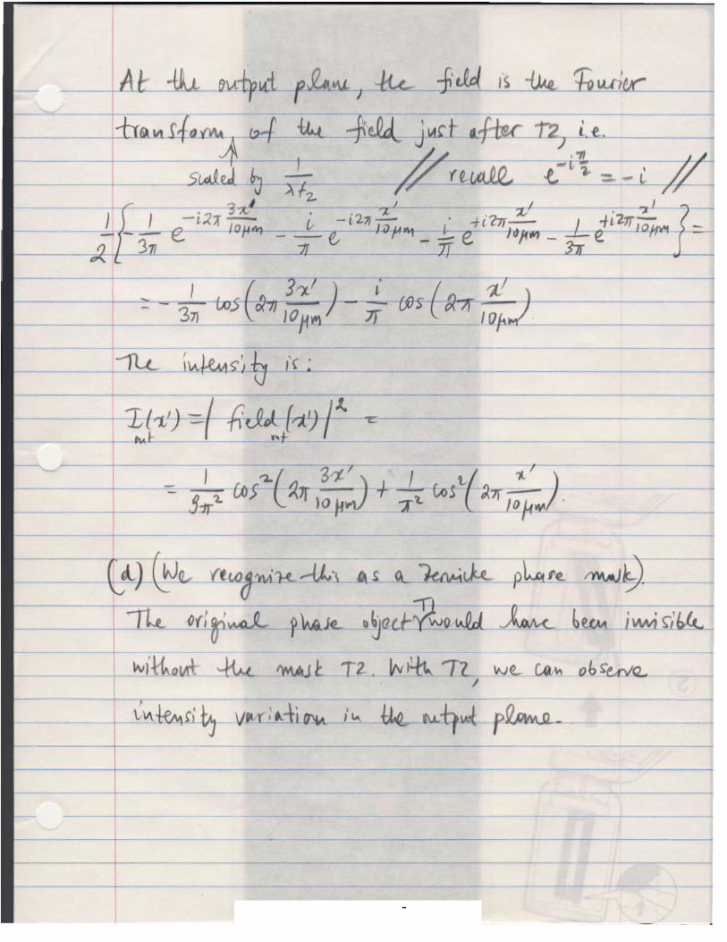
The field at the image plane is the Fourier transform of the field immediately after the grating T2, which is computed as

3 1"" "" "" "" F −sinc [δ(x − 3) + δ(x + 3)] − isinc [δ(x − 1) + δ(x + 1)] = 2 2 ''→ x ' u λf

"" "" "" "" 3 δ(x − q) + δ(x + q) 1 δ(x − 1) + δ(x + 1) − 2sinc F − 2isinc F = 2 2 2 2

3 1 −2 3x 2 x −2sinc cos (2π3u)−2isinc cos (2πu) = −2 cos 2π −2i cos 2π = 2 2 3π λf2 π λf2

4 2π 4 2π cos (0.3)x − i cos (0.1)x . (8)

3π λ π λ

3

����

� � � ������ � � �

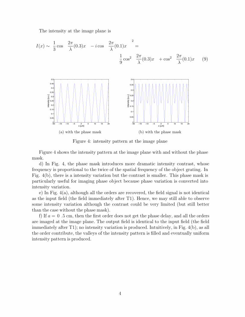
The intensity at the image plane is

1 2π 2π 2

I(x) ∼ cos (0.3)x − i cos (0.1)x = 3 λ λ

1 2π 2π cos 2 (0.3)x + cos2 (0.1)x (9)

9 λ λ

0.5 0.4

0.45

inte

nsity [

a.u

.]

0.4

0.35

0.3

0.25

0.2

0.15

0.1

0.05

0 -20 -15 -10 -5 0

0.05

0.1

0.15

0.2

0.25

0.3

0.35

inte

nsity [

a.u

.]

-20 -15 -10 -5 0 5 10 15 20 0 5 10 15 20 x [µm] x [µm]

(a) with the phase mask (b) with the phase mask

Figure 4: intensity pattern at the image plane

Figure 4 shows the intensity pattern at the image plane with and without the phase mask.

d) In Fig. 4, the phase mask introduces more dramatic intensity contrast, whose frequency is proportional to the twice of the spatial frequency of the object grating. In Fig. 4(b), there is a intensity variation but the contrast is smaller. This phase mask is particularly useful for imaging phase object because phase variation is converted into intensity variation.

e) In Fig. 4(a), although all the orders are recovered, the field signal is not identical as the input field (the field immediately after T1). Hence, we may still able to observe some intensity variation although the contrast could be very limited (but still better than the case without the phase mask).

f) If a = 0 .5 cm, then the first order does not get the phase delay, and all the orders are imaged at the image plane. The output field is identical to the input field (the field immediately after T1); no intensity variation is produced. Intuitively, in Fig. 4(b), as all the order contribute, the valleys of the intensity pattern is filled and eventually uniform intensity pattern is produced.

4

if*II I of - ltw to - PrrLupra (A ,I

f") 1!- ie "-if,oi "^^sb; +A,

t/ I - ' /vt-wlet 1l4L

a"t "AA"rU&-1t^e-

\uru' ,l gA^t ro-kui; ty

I{il l t (u*'{-)

s ctnr q^L f**e-"ff*'^o*'t

rMs ., Tt do+t

- i+ - fX.4( = ?-'S !4 tlr2{ l tn1r( fpor

pwioeieJfu -*fe'"fr Ie+utoJ= l,z yxl

0t J,^sI L,/* rt, fu

t,o "d"; - "+tl-i*fkdft c I,

r t f . I

J N nn ula L h-ad'rrusn' p t?-6 , T-' g*r<

+u!- R*aq.

tl;try +1^*^1

t,Zt IJ

=4 rr / Lr , ?zrnz

Z-fF-e-'v_=n(z)'7l rr

.t

, Wc obtqin

I ph erc lr

siJ$l i?r^*-

c-L- A

Vl'r

ro ii ?1toPractice Problem Set 3 page 20-

Another solution with an alternative definition of the grating T1

4tt|],a'ilsU'u

ltofn

o t 0^

e"T - * a]aa*4n^dtrtg

f *nr*1s&*

-dLaappgJw- -y--

I

I

I

I

-3)

f c-"?e,np ry&^v. -.- - l_..

O * r"laralfi dtrw X

,T{vr/\ T,fr ) n,'s

Practice Problem Set 3 page 21-

-'-

f,l-____ #l --

ry 7L nlt^t ytt ry i

t-tfu

- *+ {t+-+},tt

I

z+ =-ur# S,o=1f5

--5r

-t'#F

=

-Wqttat- yftTsrirp

:lr-Tryilw rLl

Practice Problem Set 3 page 22-

-a-^,,r6J 7nqffi-"HW

VM$f wq/

?ry\ -Zf%r-{-ZIffir lti-ii ^-a

- ---i

rrtv vt .} t11,l rl.,_,

i

6ry "'Tdw, "

7n4ol I-I

\ .1r --t

| ,t iAl..W-ut,

1 \rLt

:I__2

J4 l^nrrff"ry]

Practice Problem Set 3 page 23-

MIT OpenCourseWarehttp://ocw.mit.edu

2.71 / 2.710 OpticsSpring 2014

For information about citing these materials or our Terms of Use, visit: http://ocw.mit.edu/terms.