1

Optical Tracking in Medical Physics

Advanced Lab Course Experiment at the Department of Medical Physics

April 23rd, 2021

2

Index

1. Introduction 3 2. Principles of optical tracking 4 3. Principles of surface detection 9 4. Experimental methods and materials 13 5. Experimental procedure 24 6. Data analysis 31 7. References 32 8. Appendix 33

3

1. Introduction

Optical tracking systems use infrared light to determine the position of a target via active (transmits its

own infrared light) or passive (reflects infrared light supplied by an external illumination source) markers.

The most common active targets are infrared (IR) light-emitting diodes (LEDs). Passive targets are

generally spheres or disks coated with a highly reflective material. Various detectors can be used to

determine the positions of an optical target; however, charged couple device (CCD) cameras are used

most often. Each CCD camera provides a 2D image of a scene, as viewed from the specific camera angle.

An array of cameras provides a number of different views of the same scene, each from a different

perspective. The multiple views of the same scene can be used to reconstruct accurate 3D locations of

each object in the scene.

This is how an individual point object is tracked. However, the ability to track the location of a single object

by itself is not sufficient to track the location of a target (point) inside the patient. Such a goal can be

achieved by correlating the position of external marker to the 3D motion of internal targets, relying on

dedicated imaging data. In this way, optical tracking systems can be used to provide stereotactic

localization, allowing quasi real-time localization to implement motion management strategies.

An alternative approach is to detect surface information from single or multiple camera systems, relying

on infrared light projected by an illuminator. Such an approach has the advantage to avoid the placement

of markers, and directly uses the skin surface of the patient for stereotactic localization. The use of such

systems is rapidly spreading for medical physics applications in external beam radiotherapy.

4

2. Principles of optical tracking

Optical tracking provides 3D localization of specific points (markers) as a function of time, relying on

synchronized views from at least two points of view (cameras). Optical tracking systems based on IR

cameras are the actual standard in medical applications for the following main reasons:

computer vision techniques provide accurate, real-time and 3D point (marker) localization

The use of IR light minimizes disturbances due to visible light.

Visibility of the markers to be tracked needs to be ensured in order to achieve proper 3D reconstruction.

Different markers can be used, as schematized in Figure 1:

Active (cabled or wireless) markers, where the marker emits IR light to be localized by multiple

cameras

Passive markers, that reflect the IR light emitted by appropriate illumination LEDs, which operate

synchronously with respect to the acquisition frequency of the cameras.

Figure 1. Markers utilized by IR optical tracking systems.

The simplest model of a camera is the pinhole camera model: light is envisioned as entering from the

scene or a distant object, but only a single ray enters from any particular point (Figure 2). In a physical

pinhole camera, this point is then “projected” onto an imaging surface. As a result, the image on this

image plane (also called the projective plane) is always in focus, and the size of the image relative to the

distant object is given by a single parameter of the camera, its focal length f:

−𝑥 = 𝑓𝑋

𝑍

Where X is the object physical size, Z is the distance of the object from the pinhole plane and x is the

object size as visible on the projective plane

5

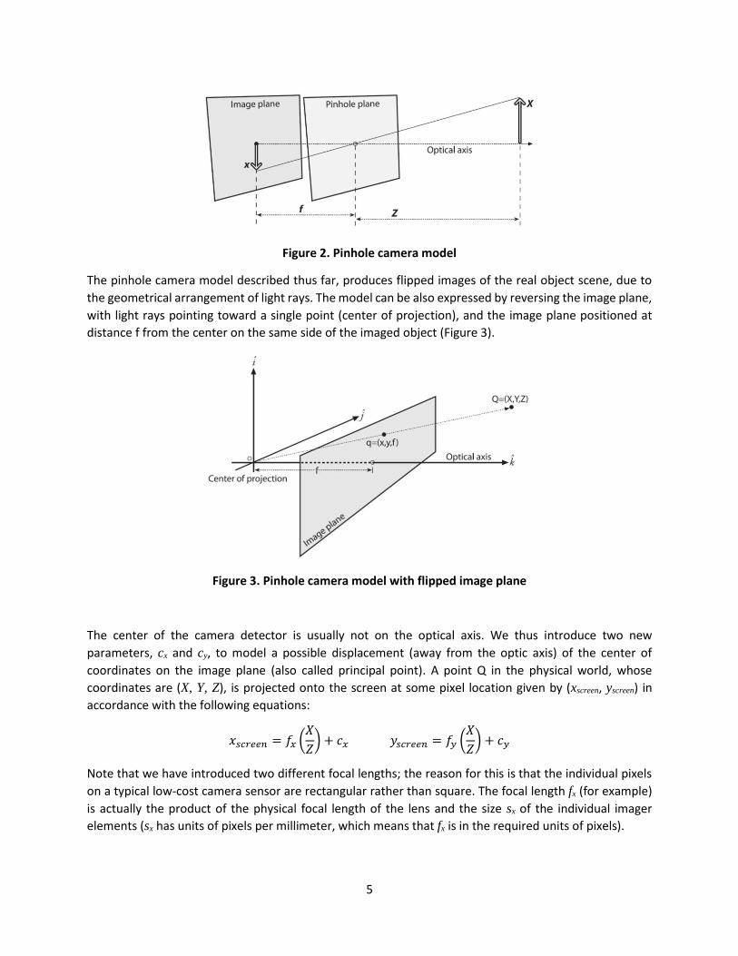
Figure 2. Pinhole camera model

The pinhole camera model described thus far, produces flipped images of the real object scene, due to

the geometrical arrangement of light rays. The model can be also expressed by reversing the image plane,

with light rays pointing toward a single point (center of projection), and the image plane positioned at

distance f from the center on the same side of the imaged object (Figure 3).

Figure 3. Pinhole camera model with flipped image plane

The center of the camera detector is usually not on the optical axis. We thus introduce two new

parameters, cx and cy, to model a possible displacement (away from the optic axis) of the center of

coordinates on the image plane (also called principal point). A point Q in the physical world, whose

coordinates are (X, Y, Z), is projected onto the screen at some pixel location given by (xscreen, yscreen) in

accordance with the following equations:

𝑥𝑠𝑐𝑟𝑒𝑒𝑛 = 𝑓𝑥 (𝑋

𝑍) + 𝑐𝑥 𝑦𝑠𝑐𝑟𝑒𝑒𝑛 = 𝑓𝑦 (

𝑋

𝑍) + 𝑐𝑦

Note that we have introduced two different focal lengths; the reason for this is that the individual pixels

on a typical low-cost camera sensor are rectangular rather than square. The focal length fx (for example)

is actually the product of the physical focal length of the lens and the size sx of the individual imager

elements (sx has units of pixels per millimeter, which means that fx is in the required units of pixels).

6

In theory, it is possible to define a lens that will introduce no distortions. In practice, however, no lens is

perfect, featuring mainly radial and tangential distortion effects. For radial distortion, the distortion is 0

at the (optical) center of the imager and increases as we move toward the periphery (Figure 4). In practice,

this distortion is small and can be characterized by the first few terms of a Taylor series expansion around

r = 0. For cheap web cameras, we generally use the first two such terms; the first of which is conventionally

called k1 and the second k2. For highly distorted cameras, such as fish-eye lenses, we can use a third radial

distortion term k3.

𝑥𝑐𝑜𝑟𝑟𝑒𝑐𝑡𝑒𝑑 = 𝑥(1 + 𝑘1𝑟2 + 𝑘2𝑟4 + 𝑘3𝑟6)

𝑦𝑐𝑜𝑟𝑟𝑒𝑐𝑡𝑒𝑑 = 𝑦(1 + 𝑘1𝑟2 + 𝑘2𝑟4 + 𝑘3𝑟6)

Figure 4. Radial distortion effects

The second-largest common distortion is tangential distortion. This distortion is due to manufacturing

defects, resulting from the lens not being exactly parallel to the imaging plane (Figure 5). Tangential

distortion is minimally characterized by two additional parameters, p1 and p2, such that:

𝑥𝑐𝑜𝑟𝑟𝑒𝑐𝑡𝑒𝑑 = 𝑥 + [2𝑝1𝑦 + 𝑝2(𝑟2 + 2𝑥2)]

𝑦𝑐𝑜𝑟𝑟𝑒𝑐𝑡𝑒𝑑 = 𝑦 + [𝑝1(𝑟2 + 2𝑦2) + 2𝑝2𝑥]

Figure 5. Tangential distortion effects (right panel), as resulting from manufacturing (left panel)

7

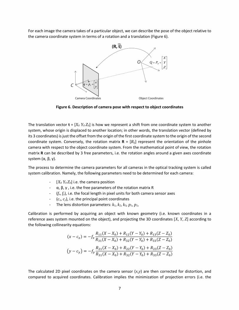
For each image the camera takes of a particular object, we can describe the pose of the object relative to

the camera coordinate system in terms of a rotation and a translation (Figure 6).

Figure 6. Description of camera pose with respect to object coordinates

The translation vector t = [X0 Y0 Z0] is how we represent a shift from one coordinate system to another

system, whose origin is displaced to another location; in other words, the translation vector (defined by

its 3 coordinates) is just the offset from the origin of the first coordinate system to the origin of the second

coordinate system. Conversely, the rotation matrix R = [Rij] represent the orientation of the pinhole

camera with respect to the object coordinate system. From the mathematical point of view, the rotation

matrix R can be described by 3 free parameters, i.e. the rotation angles around a given axes coordinate

system (α, β, γ).

The process to determine the camera parameters for all cameras in the optical tracking system is called

system calibration. Namely, the following parameters need to be determined for each camera:

- [X0 Y0 Z0] i.e. the camera position

- α, β, γ , i.e. the free parameters of the rotation matrix R

- (fx, fy), i.e. the focal length in pixel units for both camera sensor axes

- (cx, cy), i.e. the principal point coordinates

- The lens distortion parameters: k1, k2, k3, p1, p1,

Calibration is performed by acquiring an object with known geometry (i.e. known coordinates in a

reference axes system mounted on the object), and projecting the 3D coordinates [X, Y, Z] according to

the following collinearity equations:

(𝑥 − 𝑐𝑥) = −𝑓𝑥

𝑅11(𝑋 − 𝑋0) + 𝑅12(𝑌 − 𝑌0) + 𝑅13(𝑍 − 𝑍0)

𝑅31(𝑋 − 𝑋0) + 𝑅32(𝑌 − 𝑌0) + 𝑅33(𝑍 − 𝑍0)

(𝑦 − 𝑐𝑦) = −𝑓𝑦

𝑅21(𝑋 − 𝑋0) + 𝑅22(𝑌 − 𝑌0) + 𝑅23(𝑍 − 𝑍0)

𝑅31(𝑋 − 𝑋0) + 𝑅32(𝑌 − 𝑌0) + 𝑅33(𝑍 − 𝑍0)

The calculated 2D pixel coordinates on the camera sensor (x,y) are then corrected for distortion, and

compared to acquired coordinates. Calibration implies the minimization of projection errors (i.e. the

8

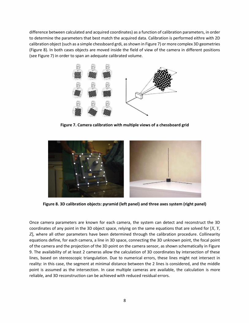
difference between calculated and acquired coordinates) as a function of calibration parameters, in order

to determine the parameters that best match the acquired data. Calibration is performed eithre with 2D

calibration object (such as a simple chessboard grdi, as shown in Figure 7) or more complex 3D geometries

(Figure 8). In both cases objects are moved inside the field of view of the camera in different positions

(see Figure 7) in order to span an adequate calibrated volume.

Figure 7. Camera calibration with multiple views of a chessboard grid

Figure 8. 3D calibration objects: pyramid (left panel) and three axes system (right panel)

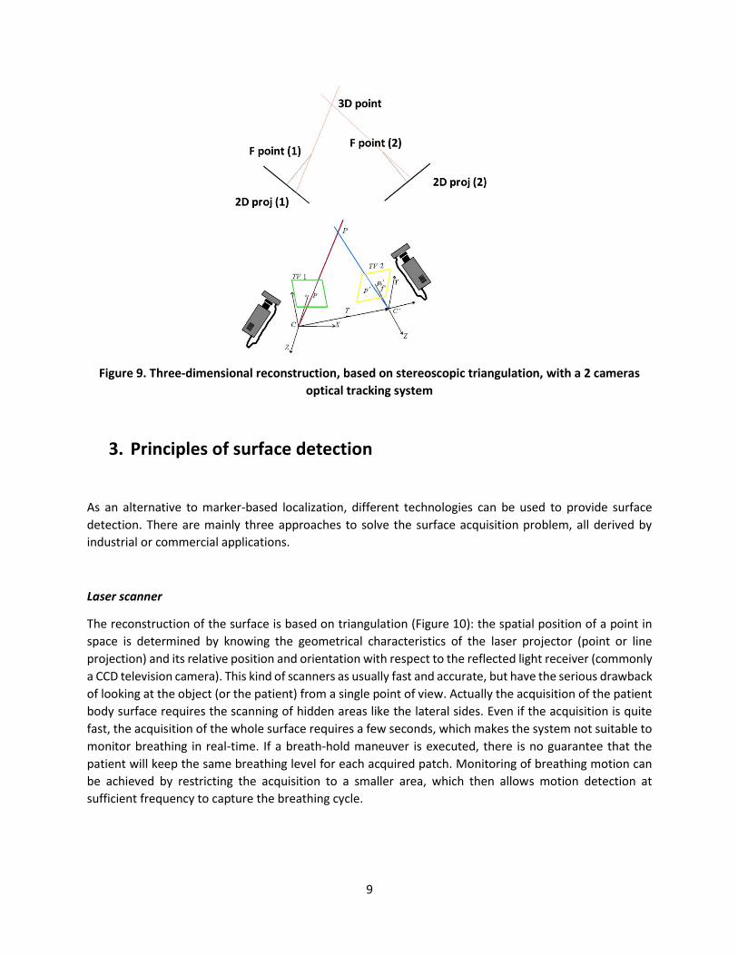
Once camera parameters are known for each camera, the system can detect and reconstruct the 3D

coordinates of any point in the 3D object space, relying on the same equations that are solved for [X, Y,

Z], where all other parameters have been determined through the calibration procedure. Collinearity

equations define, for each camera, a line in 3D space, connecting the 3D unknown point, the focal point

of the camera and the projection of the 3D point on the camera sensor, as shown schematically in Figure

9. The availability of at least 2 cameras allow the calculation of 3D coordinates by intersection of these

lines, based on stereoscopic triangulation. Due to numerical errors, these lines might not intersect in

reality: in this case, the segment at minimal distance between the 2 lines is considered, and the middle

point is assumed as the intersection. In case multiple cameras are available, the calculation is more

reliable, and 3D reconstruction can be achieved with reduced residual errors.

9

Figure 9. Three-dimensional reconstruction, based on stereoscopic triangulation, with a 2 cameras

optical tracking system

3. Principles of surface detection

As an alternative to marker-based localization, different technologies can be used to provide surface

detection. There are mainly three approaches to solve the surface acquisition problem, all derived by

industrial or commercial applications.

Laser scanner

The reconstruction of the surface is based on triangulation (Figure 10): the spatial position of a point in

space is determined by knowing the geometrical characteristics of the laser projector (point or line

projection) and its relative position and orientation with respect to the reflected light receiver (commonly

a CCD television camera). This kind of scanners as usually fast and accurate, but have the serious drawback

of looking at the object (or the patient) from a single point of view. Actually the acquisition of the patient

body surface requires the scanning of hidden areas like the lateral sides. Even if the acquisition is quite

fast, the acquisition of the whole surface requires a few seconds, which makes the system not suitable to

monitor breathing in real-time. If a breath-hold maneuver is executed, there is no guarantee that the

patient will keep the same breathing level for each acquired patch. Monitoring of breathing motion can

be achieved by restricting the acquisition to a smaller area, which then allows motion detection at

sufficient frequency to capture the breathing cycle.

10

Figure 10. Example of a laser scanner for radiotherapy applications. The projected laser light is reconstructed in 3D relying on known relative geometry between the projector and the sensor.

Fringe-pattern projector

Fringe pattern scanners (also called structured light scanners or Moiré fringes projectors) historically have

been the first qualitative tool used for surface morphology acquisition. Their first use was to define

asymmetries in body shape to quantify, for example, scoliosis level. Technological development has led

to systems able to acquire the same surface portion projecting fringe patterns at increasing spatial

frequency, in order to iteratively calculate spatial localization of the subject surface (Figure 11).

This kind of scanners have mainly the same problems of the static laser scanners, as their position relative

to the acquired object must be kept constant during the scanning procedure. Anyway, a particular

drawback affects this technology is that the color of the acquired surface is a fundamental parameter in

spatial tracking: a black or dark spot on a white background, or vice versa, is seen as a difference in depth

with respect to the acquisition field.

Figure 11. Fringe projector (A) and fringe projected on a complex surface (B)

11

Stereo-cameras

The term “stereo-cameras” commonly defines a system made up by two common photographic cameras,

rigidly connected to each other and calibrated, that shoot a picture at the same object from two different

points of view. These systems typically rely on an infrared pattern projector, which generates a pseudo-

random pattern on the surface (Figure 12). The pattern is then analyzed in the two pictures, and

correspondent points are detected via a template matching procedure. The 3D positions of such points is

then reconstructed relying on stereoscopic principles, similar to what described for marker-based optical

tracking (Figure 12). An additional RGB camera can be integrated for texture detection, which provides a

realistic representation of the detected surface.

Figure 12. Stereo-cameras system, showing the infrared pattern (left panels), the reconstructed

geometrical surface (central panel) and the stereoscopic triangulation principle (right panel)

Stereo-camera systems based on stereoscopic triangulation are now widespread for medical physics

applications in external beam radiotherapy. An alternative approach with stereo-cameras, where cameras

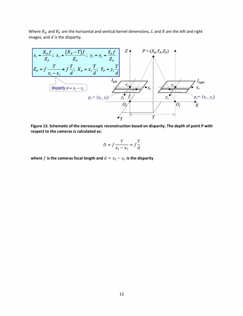
are positioned in a parallel arrangement is also possible (Figure 13). Such a configuration has been

originally proposed for gaming, and has an intrinsically lower 3D reconstruction accuracy. The

reconstruction of the patient's surface is made through a so-called disparity map which is used to define

the 3D position of each pixel on the basis of the difference in its 2D position on the two acquired images

(see Figure 13). The disparity map is defined as the distance in pixels between each point on the left image

and the corresponding one on the right image, after an image rectification process. In order to calculate

this distance, a kernel around the considered pixel of the left image is taken and is iteratively

superimposed on the right one till the correct match is found. The figure to be minimized is usually the

sum of squared distances (𝑆𝑆𝐷), calculated as:

𝑆𝑆𝐷𝑥,𝑦 = ∑ ∑ [𝐿(𝑖, 𝑗) − 𝑅(𝑖 − 𝑑, 𝑗)]2

𝑦+𝑅𝑉

𝑗=𝑦−𝑅𝑉

𝑥+𝑅𝐻

𝑖=𝑥−𝑅𝐻

12

Where 𝑅𝐻 and 𝑅𝑉 are the horizontal and vertical kernel dimensions, 𝐿 and 𝑅 are the left and right

images, and 𝑑 is the disparity.

Figure 13. Schematic of the stereoscopic reconstruction based on disparity. The depth of point P with respect to the cameras is calculated as:

𝐷 = 𝑓𝑇

𝑥𝑙 − 𝑥𝑟= 𝑓

𝑇

𝑑

where 𝑓 is the cameras focal length and 𝑑 = 𝑥𝑙 − 𝑥𝑟 is the disparity

13

4. Experimental methods and materials

4.1 Personal safety: read me first

The Hybrid Polaris Spectra position sensor (described later) is equipped with a Class2 laser that is used to

verify the center of the calibrated volume. Pay attention at not looking into the laser aperture directly

when pressing the button to activate the laser (Figure 14).

Figure 14. Frontal view of the Hybrid Polaris Spectra position sensor showing the laser activation

button and the laser aperture

The following warning is reported on the Hybrid Polaris Spectra device to warn the user (Figure 15).

Figure 15. Laser radiation warning on the Hybrid Polaris Spectra

Please pay attention when using the system, and carefully read the following safety instructions before

operating the Hybrid Polaris Spectra system:

14

4.2 Hybrid Polaris Spectra

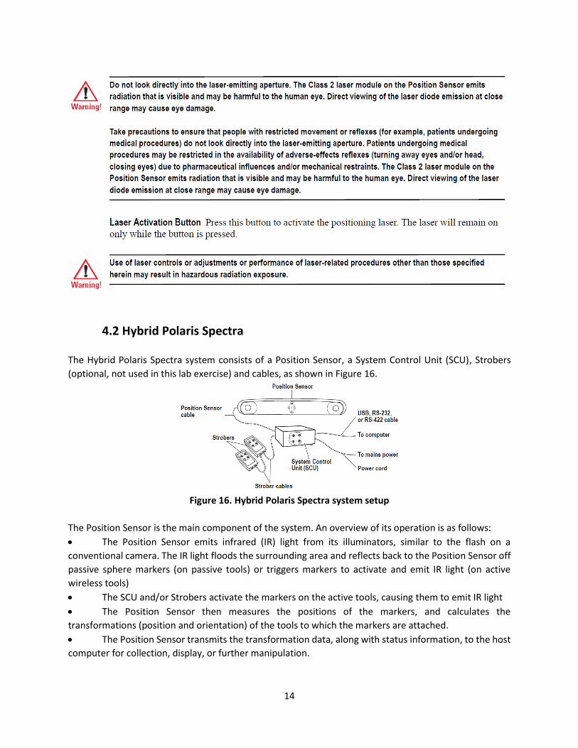
The Hybrid Polaris Spectra system consists of a Position Sensor, a System Control Unit (SCU), Strobers

(optional, not used in this lab exercise) and cables, as shown in Figure 16.

Figure 16. Hybrid Polaris Spectra system setup

The Position Sensor is the main component of the system. An overview of its operation is as follows:

The Position Sensor emits infrared (IR) light from its illuminators, similar to the flash on a

conventional camera. The IR light floods the surrounding area and reflects back to the Position Sensor off

passive sphere markers (on passive tools) or triggers markers to activate and emit IR light (on active

wireless tools)

The SCU and/or Strobers activate the markers on the active tools, causing them to emit IR light

The Position Sensor then measures the positions of the markers, and calculates the

transformations (position and orientation) of the tools to which the markers are attached.

The Position Sensor transmits the transformation data, along with status information, to the host

computer for collection, display, or further manipulation.

15

When connected to the SCU, the Position Sensor can track three types of tools: passive tools, active

wireless tools (not used in this praktikum), and active tools.

4.3 Calibrated volume

The Hybrid Polaris Spectra system provides 3D reconstruction in a reference axis system centered on the

Position sensor, as schematized in Figure 17.

Figure 17. Global coordinates system of the Hybrid Polaris Spectra system

The corresponding calibrated volume depends on system configuration. The Hybrid Polaris Spectra system

used for this lab activities features the pyramid volume as effective calibrated volume. The size of such a

calibrated volume are shown in Figure 18.

Figure 18. Calibrated volume (pyramid volume) for the Hybrid Polaris Spectra system

16

4.4 Tools and definition files

A tool is a rigid structure on which three or more markers are fixed so that there is no relative movement

between them.

Figure 19. Example of a passive tool

Passive tools (see Figure 19) are equipped with markers, which consist of plastic spheres with a reflective

IR coating, able to reflect back the IR light coming from the system cameras. Passive markers need to be

handled with care, and using gloves as depicted in Figure 20 in order to maintain the reflective coating

properties.

Figure 20. Handling of passive markers

Active tools (see Figure 21) are equipped with active LEDs, and do not require illumination from the

Position sensor to be tracked.

Figure 21. Example of an active tool

17

The system can track passive, active wireless and active tools simultaneously, with the following

restrictions:

The system can simultaneously track up to six passive tools and one active wireless tool, with the

following constraint: a maximum of 32 passive and 32 active markers, including stray markers,

can simultaneously be in view of the Positions Sensor. Additional markers in view may affect the

speed of the system and its ability to return transformations.

Up to nine active tools can be tracked simultaneously (three connected to the SCU and three

connected to each Strober).

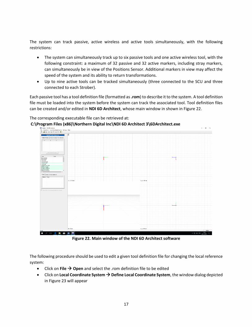
Each passive tool has a tool definition file (formatted as .rom) to describe it to the system. A tool definition

file must be loaded into the system before the system can track the associated tool. Tool definition files

can be created and/or edited in NDI 6D Architect, whose main window in shown in Figure 22.

The corresponding executable file can be retrieved at:

C:\Program Files (x86)\Northern Digital Inc\NDI 6D Architect 3\6DArchitect.exe

Figure 22. Main window of the NDI 6D Architect software

The following procedure should be used to edit a given tool definition file for changing the local reference

system:

Click on File Open and select the .rom definition file to be edited

Click on Local Coordinate System Define Local Coordinate System, the window dialog depicted

in Figure 23 will appear

18

Figure 23. Window dialog for the definition of a local reference system

Use the Edit transformation to change values and then click Apply

Click Finish to apply the selected transformation

Click on File Save As and save the edited file with an appropriate name (DO NOT OVERWRITE!).

4.5 Tracking tools

The following procedure can be used to track a specific tool with the Hybrid Polaris Spectra system:

Open the NDI Track software

The corresponding executable can be found under

C:\Program Files (x86)\Northern Digital Inc\ToolBox\Track.exe

The system will beep to establish the connection between SCU and Position Sensor

A 3D view of the acquisition volume is displayed, showing the calibrated volume and the position

of tracked tools, as shown in Figure 24

19

Figure 24. Main window of NDI Track, showing the position of a connected tool

Please note that only tools that have been pre-loaded (and positioned in the field of view) will be

visible, which includes connected active tools and wireless tools that have not been unloaded in

the previous acquisition session

Verify that connection is established on COM4 (as shown in the main window title), by checking

File Connect to

which should highlight COM4 as pre-selected

To track an active tool, plug the tool into the SCU or strober

To track a passive or active wireless tool:

o Click FileLoad Wireless Tool to load the tool definition files for the tool you want to

track

o In the dialog that appears, browse to the desired tool definition file(s). Hold down Ctrl

and click to select more than one file

o Click Open

Once a tool has been plugged in or a tool definition file has been loaded, the Hybrid Polaris Spectra

system will automatically attempt to track the tool

Move the tool throughout the characterized measurement volume, making sure the markers on

the tool face the Position sensor. As you move the tool, the symbol representing the tool in the

graphical representation will move to reflect the tool´s position.

20

A tool can be set as a reference, so that all other tools will be tracked with respect to the reference one.

To setup a tracked tool as reference, proceed as follows:

For each tool, there is a tab in the bottom right section of the NDI Track utility. Select the tab

corresponding to the tool you want to set as reference, as shown in Figure 25

Figure 25. Selection of a reference tool

Right click on the tool tab, then select Global Reference.

The reference tool will appear as a square in the graphical display. The other tools will be displayed inside

a square that is the color of the reference tool. The positions and orientations of other tools will now be

reported in the local coordinate system of the reference tool.

4.6 Pivoting tools

This section describes how to determine the tool tip offset of a probe or pointer tool by pivoting. Once

the tool tip offset is applied, the Hybrid Polaris Spectra will report the position of the tip of the tool, instead

of the position of the origin of the tool:

Setup the system to track tools, as described in the previous paragraph

Plug in (active tools) or load a tool definition file (passive and active wireless tools) for the probe

or pointer tool

For each tool, there is a tab in the bottom right section of the NDI Track utility. Select the tab

corresponding to the tool you want to pivot

Select Pivot tool

Select in the Pivot tool dialog window that appears a start delay (e.g. 5 seconds) and a duration

of about 20 seconds

Pivot the tool.

The pivoting procedure should be carried out as follows:

Place the tool tip in the hole at the center of the pivot base, as shown in Figure 26

21

Figure 26. Pivoting base

Ensure that the tool is within the characterized measurement volume, and will remain within the

volume throughout the pivoting procedure

Click Start Collection in the Pivot tool dialog

Pivot the tool in a cone shape, at an angle of 30 to 60 degrees from the vertical (Figure 27)

o Keep the tool tip stationary, and ensure that there is a line of sight between the markers

on the tool and the Position sensor throughout the pivoting procedure

o Pivot the tool slowly until the specified pivot duration time has elapsed

Figure 27. Pivoting technique

When the pivot is complete, the Pivot Result dialog appears (Figure 28). Click Apply Offset to

report the position of the tip of the tool.

Figure 28. Pivot Result dialog

22

4.7 Stray passive markers

A stray passive marker is a passive marker that is not part of a rigid body or tool. For example, by placing

stray markers on a patient´s chest, the markers may be used to gate/track the patient´s breathing in order

to achieve motion compensation in radiation therapy.

As already pointed out in the description of passive tools, stray markers should be handled with care when

they are positioned and removed, so that the reflective coating is not damaged.

When you request stray passive marker data from the Hybrid Polaris Spectra, the system will report tool

transformations, as well as 3D data (position only, no orientation information) and out-of-volume

information for up to 50 markers that are not used in tool transformations. It is then necessary to

eliminate phantom markers (i.e. undesired reflections), and verify that the stray markers are within the

characterized measurement volume.

It is important to be aware of the potential hazards associated with using the stray passive marker

reporting functionality. The hazards are as follows:

An external IR source, for example and IR transmitter of incandescent light, may be reported as a

stray marker

No marker identification is possible from frame to frame. It is therefore the user´s responsibility

to devise a method to keep track of which 3D position belongs to which marker

There are no built-in checks to determine if the 3D result is a real marker or a phantom marker,

generated by other IR sources or makers in view of the Position sensor.

Partial occlusions of markers cannot be detected or compensated for by the Position sensor. The

user may be able to detect the apparent shift if the marker position can be constrained in the

application software. For example, the marker position has to be constrained along a vector and

its position relative to another marker is supposed to be fixed within some tolerance.

In order for the Position sensor to measure stray passive markers, a tool definition file must be loaded

(which implies a passive tool is used), and the associated port handle must be initialized and enabled,

even if no tools are being tracked. The Position sensor illuminators emit IR light only when a tool definition

file is loaded.

23

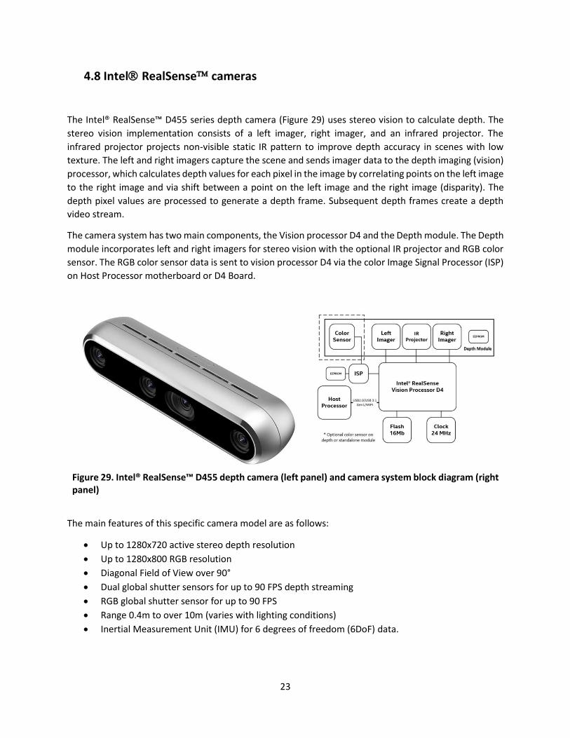
4.8 Intel RealSense cameras

The Intel® RealSense™ D455 series depth camera (Figure 29) uses stereo vision to calculate depth. The

stereo vision implementation consists of a left imager, right imager, and an infrared projector. The

infrared projector projects non-visible static IR pattern to improve depth accuracy in scenes with low

texture. The left and right imagers capture the scene and sends imager data to the depth imaging (vision)

processor, which calculates depth values for each pixel in the image by correlating points on the left image

to the right image and via shift between a point on the left image and the right image (disparity). The

depth pixel values are processed to generate a depth frame. Subsequent depth frames create a depth

video stream.

The camera system has two main components, the Vision processor D4 and the Depth module. The Depth

module incorporates left and right imagers for stereo vision with the optional IR projector and RGB color

sensor. The RGB color sensor data is sent to vision processor D4 via the color Image Signal Processor (ISP)

on Host Processor motherboard or D4 Board.

Figure 29. Intel® RealSense™ D455 depth camera (left panel) and camera system block diagram (right panel)

The main features of this specific camera model are as follows:

Up to 1280x720 active stereo depth resolution

Up to 1280x800 RGB resolution

Diagonal Field of View over 90°

Dual global shutter sensors for up to 90 FPS depth streaming

RGB global shutter sensor for up to 90 FPS

Range 0.4m to over 10m (varies with lighting conditions)

Inertial Measurement Unit (IMU) for 6 degrees of freedom (6DoF) data.

24

5. Experimental procedure

The following preliminary operations should be performed for the Hybrid Polaris before acquisition:

Switch on power in the Hybrid Polaris Spectra system, with the switch positioned on the rear part

of the SCU (Figure 30)

Figure 30. Rear panel of the SCU, with the power button on the left side of the power cable

The SCU and the Position sensor will beep in a sequence

Wait for system to be ready: the two green LEDs on the Position sensor will stop flashing. When

they are both on and green the system is ready (Figure 31)

Figure 31. Position sensor, showing the steady green LEDs on (center of the device) for correct

system operation

Please report any anomalous behavior before continuing with the next steps, as this might compromise

the reliability of your measurements and/or the system itself.

25

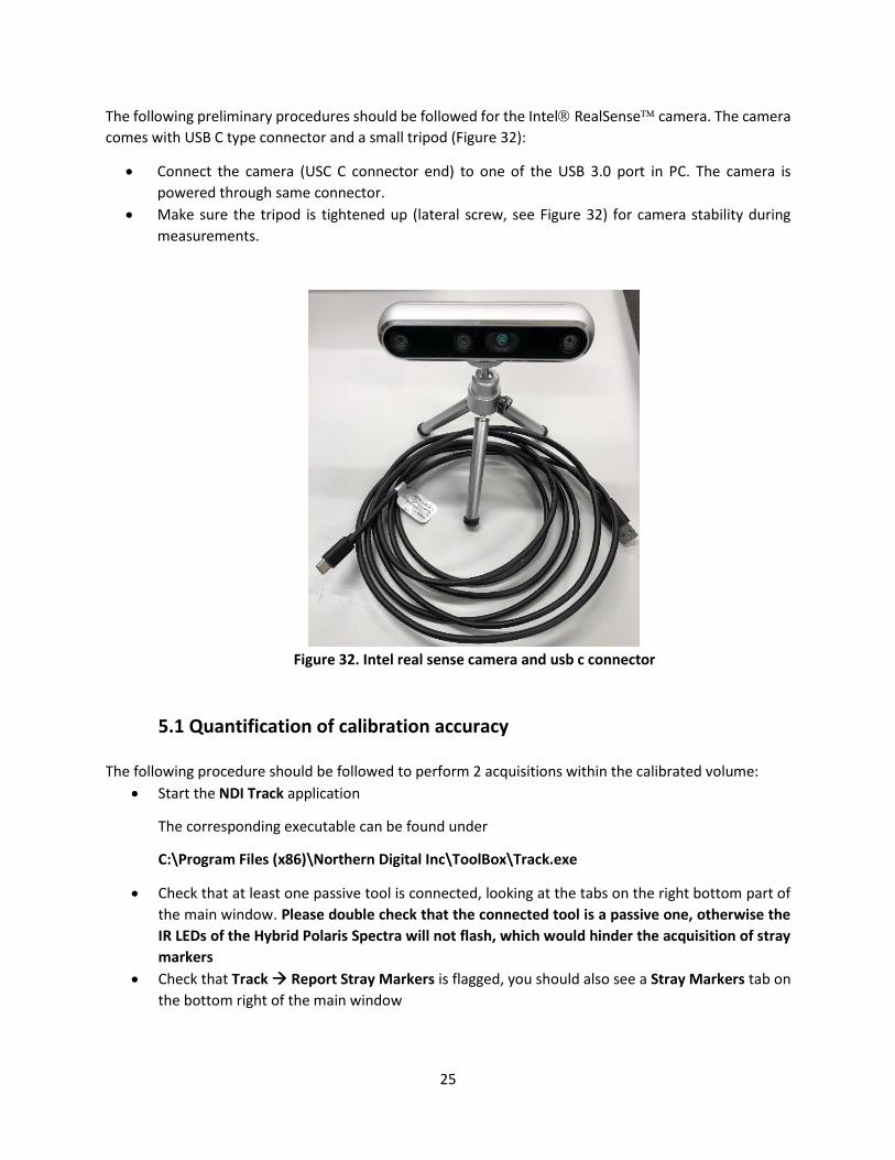
The following preliminary procedures should be followed for the Intel RealSense camera. The camera

comes with USB C type connector and a small tripod (Figure 32):

Connect the camera (USC C connector end) to one of the USB 3.0 port in PC. The camera is

powered through same connector.

Make sure the tripod is tightened up (lateral screw, see Figure 32) for camera stability during

measurements.

Figure 32. Intel real sense camera and usb c connector

5.1 Quantification of calibration accuracy

The following procedure should be followed to perform 2 acquisitions within the calibrated volume:

Start the NDI Track application

The corresponding executable can be found under

C:\Program Files (x86)\Northern Digital Inc\ToolBox\Track.exe

Check that at least one passive tool is connected, looking at the tabs on the right bottom part of

the main window. Please double check that the connected tool is a passive one, otherwise the

IR LEDs of the Hybrid Polaris Spectra will not flash, which would hinder the acquisition of stray

markers

Check that Track Report Stray Markers is flagged, you should also see a Stray Markers tab on

the bottom right of the main window

26

Check that tracking in ON: the Frame counter on the bottom right is continuously increasing. In

case tracking is not active, press the Play button or click on Track Resume Tracking

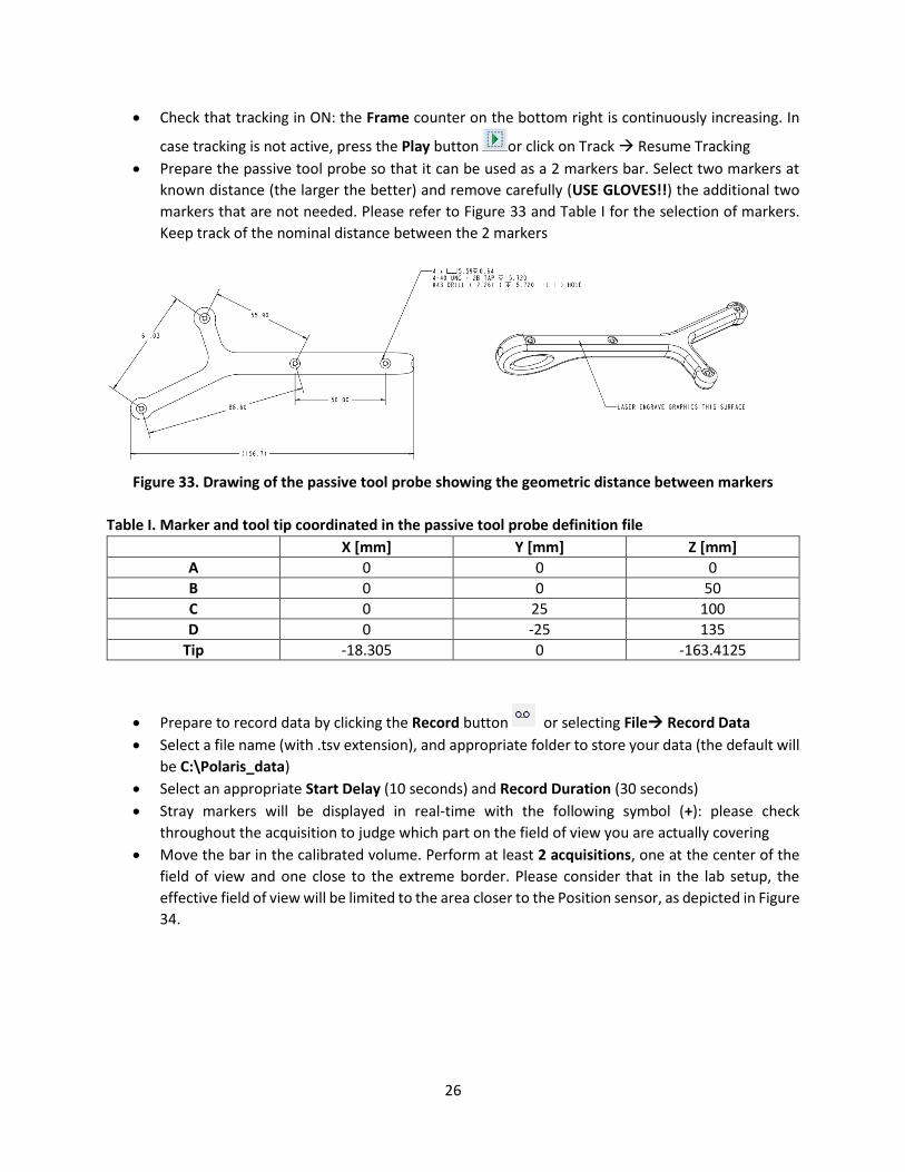
Prepare the passive tool probe so that it can be used as a 2 markers bar. Select two markers at

known distance (the larger the better) and remove carefully (USE GLOVES!!) the additional two

markers that are not needed. Please refer to Figure 33 and Table I for the selection of markers.

Keep track of the nominal distance between the 2 markers

Figure 33. Drawing of the passive tool probe showing the geometric distance between markers

Table I. Marker and tool tip coordinated in the passive tool probe definition file

X [mm] Y [mm] Z [mm]

A 0 0 0

B 0 0 50

C 0 25 100

D 0 -25 135

Tip -18.305 0 -163.4125

Prepare to record data by clicking the Record button or selecting File Record Data

Select a file name (with .tsv extension), and appropriate folder to store your data (the default will

be C:\Polaris_data)

Select an appropriate Start Delay (10 seconds) and Record Duration (30 seconds)

Stray markers will be displayed in real-time with the following symbol (+): please check

throughout the acquisition to judge which part on the field of view you are actually covering

Move the bar in the calibrated volume. Perform at least 2 acquisitions, one at the center of the

field of view and one close to the extreme border. Please consider that in the lab setup, the

effective field of view will be limited to the area closer to the Position sensor, as depicted in Figure

34.

27

Figure 34. Useful calibrated volume in the laboratory setup (shaded red area)

5.2 Reference phantom acquisition (intel-sense + Polaris)

The purpose of this procedure is to acquire a reference position for the male torso phantom (Figure 35).

The following tasks should be carried out for acquisition with the Hybrid Polaris system:

Start the NDI Track application

The corresponding executable can be found under

C:\Program Files (x86)\Northern Digital Inc\ToolBox\Track.exe

Check that the active tool (Figure 21) is connected to the SCU

Check that one of the passive tools is connected to the software application. If not, follow the

procedure described in paragraph 3.5 to connect it (using the tool definition file 8700339.rom or

8700340.rom, that can be found in C:\Optical_tracking_praktikum\tracking_tool). This is

required to activate the tracking options for stray markers

Position the pivoting stage in the FOV, and check whether pivoting (see paragraph 4.6) is feasible

in that position

Pivot the active tool as described in 4.6, so that the probe tip is reported

Check that Track Report Stray Markers is flagged in the Hybrid Polaris software, you should

also see a Stray Markers tab on the bottom right of the main window

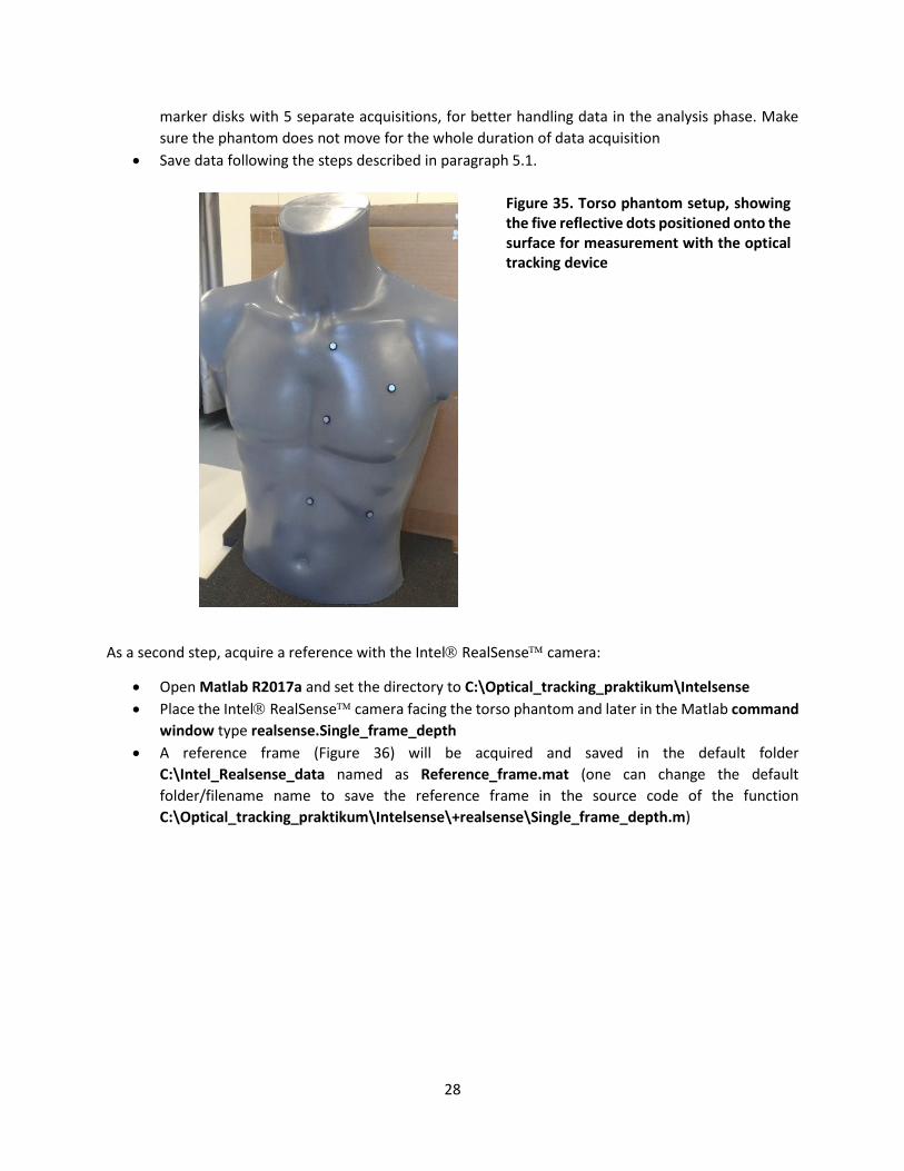
Position the torso phantom (Figure 35) in a reference position, making sure that the Hybrid Polaris

covers the surface areas corresponding to the reflective markers (the reflective coating of the

marker disks will be detected as stray marker)

Make a short acquisition (5-10 s) for the stray markers, making sure that at least 4 out of 5 are

visible

Track the reflective marker disks while sweeping the round border with the active tool, which has

a round tip. Pay attention to keep the tool tip in contact with the border, at an inclination so that

the active tool is correctly localized with the Hybrid Polaris. SUGGESTION: acquire the 5 reflective

28

marker disks with 5 separate acquisitions, for better handling data in the analysis phase. Make

sure the phantom does not move for the whole duration of data acquisition

Save data following the steps described in paragraph 5.1.

Figure 35. Torso phantom setup, showing the five reflective dots positioned onto the surface for measurement with the optical tracking device

As a second step, acquire a reference with the Intel RealSense camera:

Open Matlab R2017a and set the directory to C:\Optical_tracking_praktikum\Intelsense

Place the Intel RealSense camera facing the torso phantom and later in the Matlab command

window type realsense.Single_frame_depth

A reference frame (Figure 36) will be acquired and saved in the default folder

C:\Intel_Realsense_data named as Reference_frame.mat (one can change the default

folder/filename name to save the reference frame in the source code of the function

C:\Optical_tracking_praktikum\Intelsense\+realsense\Single_frame_depth.m)

29

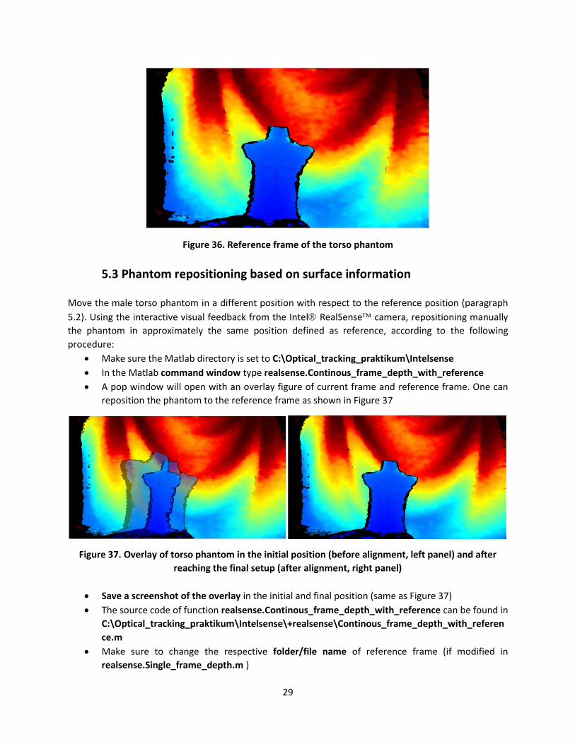
Figure 36. Reference frame of the torso phantom

5.3 Phantom repositioning based on surface information

Move the male torso phantom in a different position with respect to the reference position (paragraph

5.2). Using the interactive visual feedback from the Intel RealSense camera, repositioning manually

the phantom in approximately the same position defined as reference, according to the following

procedure:

Make sure the Matlab directory is set to C:\Optical_tracking_praktikum\Intelsense

In the Matlab command window type realsense.Continous_frame_depth_with_reference

A pop window will open with an overlay figure of current frame and reference frame. One can

reposition the phantom to the reference frame as shown in Figure 37

Figure 37. Overlay of torso phantom in the initial position (before alignment, left panel) and after

reaching the final setup (after alignment, right panel)

Save a screenshot of the overlay in the initial and final position (same as Figure 37)

The source code of function realsense.Continous_frame_depth_with_reference can be found in

C:\Optical_tracking_praktikum\Intelsense\+realsense\Continous_frame_depth_with_referen

ce.m

Make sure to change the respective folder/file name of reference frame (if modified in

realsense.Single_frame_depth.m )

30

Note: The default time for continuous frame acquisition is set to 10 minutes approx. but one can

change this time in the function C:\Optical_tracking_praktikum\Intelsense\+realsense\

Continous_frame_depth_with_reference.m

Once the final position has been reached, save the corresponding data with the Hybrid Polaris according

to the same procedure used in paragraph 5.2.

31

6. Data analysis

6.1 Quantification of calibration accuracy

Calibration accuracy should be calculated and reported as follows:

Read the acquisitions using the read_stray_markers.m script, which will be available in

C:\Optical_tracking_praktikum\m-files (edit the max_markers variable to take into account that

2 markers are expected max_markers = 2)

Calculate the standard deviation and 95th percentile of distance between markers (variable delta,

as reported and plotted by the script)

Compare such results with the nominal distance, as calculated in paragraph 5.1

Report calibration accuracy in the center of the field of view vs. close to the border

6.2 Quantification of phantom repositioning accuracy Proceed as follows to localize the phantom in the reference position:

Read the reference acquisitions using the read_tool.m script, which will be available in

C:\Optical_tracking_praktikum\m-files

Verify the measurement error, as reported by the optical tracking system in the variable err:

please check that the maximum error is below 0.15 mm

In case the maximum error exceeds the 0.15 mm threshold, filter out points whose error is larger

(point coordinates are stored in the variable data): if remaining points are sufficient to

characterize the reflective marker disk proceed, otherwise repeat the measurement as described

in paragraph 5.2

Quantify the centroid of the acquired circle trajectory, representing the center of the reflective

marker. Please take into account partial acquisitions (i.e. leading to a shifted average position)

and the fact that the active marker tool tip has a 3 mm diameter

Read the acquisitions using the read_stray_markers.m script, which will be available in

C:\Optical_tracking_praktikum\m-files (edit the max_markers variable to take into account that

5 markers are expected max_markers = 5)

Compare the reference marker locations, considering that the reflective markers have a thickness

of 3 mm

Repeat the previous steps for the acquisition relative to paragraph 5.3, thus characterizing the

phantom position after manual repositioning based on surface information.

Finally, quantify the repositioning accuracy by comparing the two acquisitions, and interpret the

obtained results.

32

7. References

Wagner TH, Meeks SL, Bova FJ, Friedman WA, Willoughby TR, Kupelian PA, Tome W. Optical

tracking technology in stereotactic radiation therapy. Med Dosim. 2007 Summer;32(2):111-20

Bert C, Metheany KG, Doppke K, Chen GT. A phantom evaluation of a stereo-vision surface

imaging system for radiotherapy patient setup. Med Phys. 2005 Sep;32(9):2753-62

Walter F, Freislederer P, Belka C, Heinz C, Söhn M,Roeder F. Evaluation of daily patient positioning

for radiotherapy with a commercial 3D surface-imaging system (Catalyst™). Radiat Oncol. 2016

Nov 24;11(1):154

Northern Digital Inc., Hybrid Polaris Spectra User Guide, Revision 5, June 2013

Fielding AL, Pandey AK, Jonmohamadi Y, Via R, Weber DC, Lomax AJ, Fattori G. Preliminary study

of the Intel RealSenseTM D415 camera for monitoring respiratory like motion of an irregular

surface. IEEE Sensors Journal, doi: 10.1109/JSEN.2020.2993264.

https://www.intel.com/content/www/us/en/architecture-and-technology/realsense-

overview.html

33

Appendix

read_tool.m

close all;

clear all;

serial_number='34801403'; %Polaris serial number

data_file='new_praktikum_01.tsv';

%read file

S=importdata(data_file,'\t');

%...GET TOOL...........................................

n_frame=zeros(size(S.textdata,1)-1,2);

data=NaN*ones(size(S.textdata,1)-1,3);

err=NaN*ones(size(S.textdata,1)-1,1);

n_tools=str2double(S.textdata(2,1));

% skip_cells=1+16*(n_tools-1)+13;

format_header='%s';

for k=1:size(S.textdata,2)-1

format_header=strcat(format_header,'%s');

end

format_data=format_header;

for k=1:n_tools

format_data=strcat(format_data,'%s%s%s%s');

end

FID = fopen(data_file);

H = textscan(FID,format_header,1); %read the header

ind_tool=[];

for k=1:length(H)

if strcmp(H{k},'Tx')==1

ind_tool=[ind_tool;k];

end

end

temp=fgetl(FID); %empty line

for i=2:size(S.textdata,1) %potential correct frames (from 2 to end of file)

temp=str2double(S.textdata(i,3));

if mod(temp,1)==0 %check if the frame number is an integer value (valid

frames)

n_frame(i-1,1)=temp;

% temp=textscan(FID,format_data,1);

temp=fgetl(FID); %empty line

temp2=strsplit(temp);

if strcmp(temp2{9},'OK')==1 %check if tool has been detected

data(i-1,1)=str2num(temp2{ind_tool(1)}); %13 to 16

data(i-1,2)=str2num(temp2{ind_tool(1)+1});

data(i-1,3)=str2num(temp2{ind_tool(1)+2});

err(i-1,1)=str2num(temp2{ind_tool(1)+3});

else

n_frame(i-1,1)=NaN;

end

else

n_frame(i-1,1)=NaN;

end

34

end

fclose(FID);

...END (GET TOOL)......................................

%PLOT

close all;

plot3(data(:,1),data(:,2),data(:,3),'.');

xlabel('X');

ylabel('Y');

zlabel('Z');

axis equal;

ok_err=find(~isnan(err));

if ~isempty(ok_err)

figure

hist(err);

end

read_stray_markers.m

close all;

clear all;

serial_number='34801403'; %Polaris serial number

data_file='phantom3.tsv';

max_markers=5; %maximum number of stray markers

%read file

S=importdata(data_file,'\t');

%...GET STRAY MARKERS..................................

n_frame=zeros(size(S.textdata,1)-1,2);

stray_markers=NaN*ones(size(S.textdata,1)-1,max_markers,3);

n_tools=str2double(S.textdata(2,1));

% skip_cells=1+16*(n_tools-1)+13;

format_header='%s';

% for k=1:(skip_cells+4*max_markers)-1

for k=1:size(S.textdata,2)-1

format_header=strcat(format_header,'%s');

end

FID = fopen(data_file);

H = textscan(FID,format_header,1); %read the header

temp=fgetl(FID); %empty line

for i=2:size(S.textdata,1) %potential correct frames (from 2 to end of file)

temp=str2double(S.textdata(i,3));

if mod(temp,1)==0 %check if the frame number is an integer value (valid

frames)

n_frame(i-1,1)=temp;

temp=fgetl(FID); %get next line (number of entries vary depending on

tool status

ind_OK=strfind(temp,'OK');

35

ind_OK=[ind_OK,size(temp,2)];

if length(ind_OK)>max_markers %>=

ind_OK=ind_OK(end-max_markers:end);

for k=1:(max_markers)

data_k=temp(ind_OK(k)+2:ind_OK(k+1)-1);

data_temp=str2num(data_k);

if length(data_temp)>0

stray_markers(i-1,k,1)=data_temp(1); %X

stray_markers(i-1,k,2)=data_temp(2); %Y

stray_markers(i-1,k,3)=data_temp(3); %Z

else

stray_markers(i-1,k,1)=NaN;

stray_markers(i-1,k,2)=NaN;

stray_markers(i-1,k,3)=NaN;

end

end

end

else

n_frame(i-1,1)=NaN;

end

end

fclose(FID);

%...END(GET STRAY MARKERS)...........................

%PLOT

figure;

x=stray_markers(:,:,1);

y=stray_markers(:,:,2);

z=stray_markers(:,:,3);

for k=1:max_markers

plot3(x(:,k),y(:,k),z(:,k),'.');

hold on

end

axis equal

Single_frame_depth.m

function Single_frame_depth() % Make Pipeline object to manage streaming pipe = realsense.pipeline(); % Make Colorizer object to prettify depth output colorizer = realsense.colorizer();

% Start streaming on an arbitrary camera with default settings profile = pipe.start();

% Get streaming device's name dev = profile.get_device(); name = dev.get_info(realsense.camera_info.name);

% Get frames. We discard the first couple to allow % the camera time to settle

36

for i = 1:15 fs = pipe.wait_for_frames(); end

% Stop streaming pipe.stop();

% Select depth frame depth = fs.get_depth_frame(); % Colorize depth frame color = colorizer.colorize(depth);

% Get actual data and convert into a format imshow can use % (Color data arrives as [R, G, B, R, G, B, ...] vector) data = color.get_data(); img = permute(reshape(data',[3,color.get_width(),color.get_height()]),[3

2 1]);

% Display image imshow(img); title(sprintf("Reference depth frame from %s", name));

% Path and filename for saving reference frame % Change to desired file location/name save(['C:\Intel_Realsense_data\Reference_frame'],'img','-v7.3') end

Continous_frame_depth_with_reference.m

function Continous_frame_depth_with_reference()

% Make Pipeline object to manage streaming pipe = realsense.pipeline(); % Make Colorizer object to prettify depth output colorizer = realsense.colorizer();

% Image_reference_frame=uint8(ones(480,848,3));

% % % Loading Reference frame

Image_reference_frame=load('C:\Intel_Realsense_data\Reference_frame.mat'); % Start streaming on an arbitrary camera with default settings profile = pipe.start(); figure('visible','on'); hold on; % Get streaming device's name dev = profile.get_device(); name = dev.get_info(realsense.camera_info.name);

% Main loop % for i = 1:1000 for ~119sec % for i = 1:5000 for ~10mins

37

% for i = 1:10000 for ~20mins tic for i = 1:5000

% Obtain frames from a streaming device fs = pipe.wait_for_frames();

% Select depth frame depth = fs.get_depth_frame(); %color = fs.get_color_frame(); color = colorizer.colorize(depth); data = color.get_data(); depth_rgb=fs.get_color_frame(); color_rgb=depth_rgb; data_rgb = color_rgb.get_data(); % Depth frame img =

permute(reshape(data',[3,color.get_width(),color.get_height()]),[3 2 1]); % Rgb_frame img_rgb =

permute(reshape(data_rgb',[3,color_rgb.get_width(),color_rgb.get_height()]),[

3 2 1]); hold off;

%Skipping inital few frames to allow the camera time to settle if i>15 % Image_reference_frame=im2bw(rgb2gray(img),0.05); % % % % Difference of realtime frame Vs reference frame

imshowpair(img,Image_reference_frame.img,'blend','Scaling','joint') % % current depth frame % imshow(img); % % current RGB frame % imshow(img_rgb); pause(0.01); else

%

end % pcshow(vertices); Toolbox required end toc % Stop streaming pipe.stop();

end