optical frequency domain reflectometry: sensing...
TRANSCRIPT
i
Optical Frequency Domain Reflectometry: sensing
range extension and enhanced temperature sensitivity
by
Jia Song
Thesis submitted to the
Faculty of Graduate and Postdoctoral Studies
In partial fulfillment of the requirements for the
M.Sc. degree in Physics
Ottawa-Carleton Institute for Physics
University of Ottawa
Ottawa, Canada
© Jia Song, Ottawa, Canada, 2014

ii
To my family
iii
Abstract
Optical fiber sensors have attracted tremendous attention over last two decades and
have been successfully employed in various sensing applications, including
temperature, strain, current, and so on. Among all types of optical fiber sensors,
optical frequency domain reflectometry (OFDR) has been widely studied for its
merits of simple configurations, high spatial resolution and high sensing accuracy.
However, current limitation on OFDR lies in the sensing range and sensing accuracy.
The state of art performance of commercial OFDR provides ~70m sensing range as
well as 0.1K temperature accuracy. This is not adequate for large building distributed
health monitoring due to the limited sensing range. Besides, high temperature
response is also on demand for high precision measurement. To resolve the above
limitation, in this thesis two major subjects have been studied regarding improving the
performance and applicability of OFDR: One aims at extending the sensing range of
OFDR while the other one focuses on enhancing temperature sensitivity of OFDR.
Firstly, we proposed novel data resampling approach regarding tuning nonlinearities
of laser source to extend the sensing range. Commercial OFDR employs auxiliary
interferometer (AI) to trigger data acquisition, where the maximum sensing range is
limited to a quarter of the optical path difference (OPD) of AI according to Nyquist
Sampling theorem. By employing the data resampling algorithm, the sensing range is
no longer restricted by OPD and can even reach laser coherent length since OFDR is
based on coherent detection scheme. Three data resampling algorithms are
iv
individually discussed and a sensing range of ~300m (~4 times the sensing range of
commercial OFDR) with 8cm spatial resolution is for the first time achieved.
Secondly, the temperature response of OFDR is enhanced and we successfully
achieved high temperature accuracy distributed sensing. One advantage of high
temperature response is to enhance the spatial resolution since less spatial points are
required in performing cross-correlation, while the other advantage is to obtain high
temperature accuracy measurement at the same spatial resolution compared to that of
traditional OFDR. This is especially important for maintaining spatial resolution
under long range OFDR sensing since the total wavelength tuning range is smaller
than traditional OFDR. Commonly the temperature response of single mode fiber is
contributed by both thermal expansion coefficient and thermal optic coefficient of the
waveguide and can be enhanced by increasing either of those coefficients. Thermal
expansion coefficient is related with material property and is a weighted value of both
bare fiber and coating. By using a large thermal expansion coefficient acrylic plank as
a “coating” on SMF, we achieved ~9 times temperature response (~95 pm/ ˚C)
compared with SMF (~10 pm/ ˚C). Further experiment is demonstrated with small
diameter taper on an acrylic plank “coating”, in which case both thermal expansion
coefficient and thermal optic coefficient are raised and a ~20 times temperature
response than SMF (~200 pm/˚C) is obtained. This is especially meaningful for its
easy fabrication, low cost and extremely high temperature response and leads to
practical usage for high accuracy distributed temperature sensing.
v
Acknowledgement
It is my great honor to thank all people who have encouraged and helped me during
my master’s studies.
First of all, I would thank my supervisor, Professor Xiaoyi Bao for endowing me this
opportunity to have my master study in her group. Prof. Bao, with her critical thinking,
profound knowledge in physics and creative ideas, deeply impressed me. Her
perseverance and dedication set me a good example for doing research. Her insightful
instructions and valuable revisions helped and inspired me for fulfilling my research
topics. This thesis would be impossible without her constant support and guidance. I
would also express my gratitude to Professor Liang Chen, his precious help,
meaningful suggestions and detailed revision helped improving the quality of this
thesis.
Secondly, I shall thank Dr. Ping Lu for his detailed guidance, useful instructions and
precise modification. I gained deep understanding in fiber optics and was able to find
suitable research topics through discussions with him.
I also thank Dr. Wenhai Li for his efforts helping me with the OFDR configuration;
this project cannot be fulfilled without whose early explorations.
Many thanks are given to Mr. Yanping Xu, who not only helped me in lab but also in
daily lives. His strong motivation and optimism inspired me when I was low. I shall
give special thanks to Yang Lu. His comments and advices helped improving the
performance of OFDR system. I would also thank Dr. Zengguang Qin for his

vi
meaningful instructions and assistance in research topics and daily lives.
I am thankful to all other colleagues in this lab: Dr. Chams Baker, Dr. Zhonghua Ou,
Mr. Yang Li, Mr. Bhavaye Saxena, Dr. Meng Pang, Dr. Xiaozhen Wang, Dr. Dapeng
Zhou, Ms. Daisy Williams, Ms. Meiqi Ren, Mr. Dao Xiang and Mr. Hugo Larocque.
Lastly, I shall sincerely thank my family and my best friends, for their support,
anticipation, encouragement and comforts. I shall never forget your blessing and
comforting me in those tough times, which set up my resolution to pursue this life.
I would also like to thank Collaborative Research and Training Experience Program
(CREATE) program by Natural Sciences and Engineering Research Council of
Canada (NSERC) that supported me for the entire master study.

vii
Statement of originality
This work contains no material which has been accepted for the award of any
other degree or diploma in any university or other tertiary institution and, to the best
of my knowledge and belief, contains no material previously published or written by
another person, except where due reference has been made in the text.
I give consent to this copy of my thesis, when deposited in the University Library,
being available for loan and photocopying.
SIGNED: ………………………………..
DATE: …………………………………...
Supervisors: Prof. Xiaoyi Bao
viii
Contents
Abstract ....................................................................................................................... iii
Acknowledgement ........................................................................................................ v
List of Figures ............................................................................................................... x
List of Tables ............................................................................................................ xiii
List of Acronyms ....................................................................................................... xiv
1. Introduction .............................................................................................................. 1
1.1 Background and Motivation ........................................................................................... 1
1.2 Thesis contribution ......................................................................................................... 5
1.3 Thesis outline ................................................................................................................. 8
2. Distributed fiber sensor and principle of OFDR .................................................. 9
2.1 Distributed fiber optical sensors ..................................................................................... 9
2.1.1 Rayleigh Scattering based Distributed Sensor ....................................................... 12
2.1.2 Optical Time Domain Reflectometry (OTDR) ...................................................... 14
2.2 Theory of OFDR........................................................................................................... 18
2.2.1 Fundamental theory of OFDR with two electrical fields........................................ 18
2.2.2 Fundamental Theory of OFDR with polarization diversity scheme ....................... 21
2.2.3 Distributed Temperature and Strain sensing based on OFDR ................................ 33
2.2.4 Sensing resolution vs. spatial resolution ................................................................ 35
3. Extended sensing length of OFDR........................................................................ 40
3.1 Introduction .................................................................................................................. 40
3.2 Frequency Tuning Nonlinearity Compensation by Using Non-Uniform FFT (NUFFT)
........................................................................................................................................... 41
3.2.1 Theory of NU-FFT ................................................................................................ 42
3.2.2 Experimental Result on Simulation data ................................................................ 45
3.2.3 Experimental Result on Real data .......................................................................... 47
3.2.4 Limitations of NU-FFT .......................................................................................... 49
3.3 Frequency Tuning Nonlinearity Compensation by Using Deskew Filter ...................... 50
3.3.1 Theory of Deskew filter ......................................................................................... 51
ix
3.3.2 Experiment Result on Simulation data ................................................................... 54
3.3.3 Experiments based on Real data ............................................................................ 57
3.3.4 Limitations on Physics ........................................................................................... 59
3.4 Cubic Spline Interpolation ............................................................................................ 60
3.4.1 Theory of Cubic spline interpolation ..................................................................... 60
3.4.2 Applying cubic spline interpolation in data resampling ......................................... 63
3.4.3 Experimental details .............................................................................................. 65
3.4.4 Experimental results and discussion ...................................................................... 67
4. Enhanced Temperature Response Sensing based on OFDR ............................. 75
4.1 Review and Principle of temperature sensing ............................................................... 75
4.2 Enhanced temperature sensitivity based on OFDR with SMF ...................................... 76
4.2.1 Principle of enhancing temperature response ......................................................... 76
4.2.2 Experiment Set-up ................................................................................................. 76
4.2.3 Experimental Result and Discussion ...................................................................... 78
4.2.4 Thermal expansion coefficient measurement based on OFDR .............................. 80
4.3 Taper based distributed temperature sensing using OFDR ........................................... 82
4.3.1 Introduction and Properties of Taper ..................................................................... 82
4.3.2 Principle of Enhanced temperature response using taper ....................................... 84
4.3.3 Experiment Set-up ................................................................................................. 84
4.3.4 Experimental Result and Discussion ...................................................................... 85
5. Summary and Future Works ................................................................................ 89
5.1 Summary ...................................................................................................................... 89
5.2 Future Works ................................................................................................................ 90
Bibliography ............................................................................................................... 92
Curriculum Vitae ....................................................................................................... 97
Publications ................................................................................................................ 98
x
List of Figures
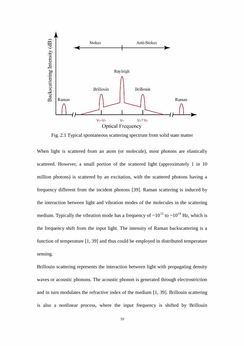
Fig. 2.1 Typical spontaneous scattering spectrum from solid state matter .................. 10
Fig. 2.2 Typical set-up of OTDR ................................................................................. 14
Fig. 2.3 Illustration of typical OTDR trace .................................................................. 15
Fig. 2.4 Schematic set-up of traditional OFDR system ............................................... 18
Fig. 2.5 Illustration of OFDR set-up with polarization diversity scheme .................... 22
Fig. 3.1 Real data of recovered (a) instantaneous optical frequency and (b)
instantaneous optical frequency increment .................................................................. 43
Fig. 3.2 OTDR-like trace (a) before NU-FFT (b) nonlinear instantaneous phase and (c)
after NU-FFT ....................................................................................................... 46
Fig. 3.3 Real data OTDR-like trace (a) before NU-FFT and (b) after NU-FFT .......... 48
Fig. 3.4 Function Generator written in LabView ......................................................... 55
Fig. 3.5 Experiments result on simulation data. (a) simulated one Fresnel reflection
point with no nonlinear term (b) simulated one Fresnel reflection point with
nonlinear term (c) simulated one Fresnel reflection point compensated by
Deskew filter ........................................................................................................ 56
Fig. 3.6 Deskew filter to compensate the nonlinearity in simulated data written in
LabView ............................................................................................................... 56
Fig. 3.7 Deskew filter to compensate the nonlinearity in real data with a nonlinear
phase prediction subroutine ................................................................................. 57
Fig. 3.8 Real data OTDR-like trace (a) before Deskew filter and (b) after Deskew
filter ...................................................................................................................... 58
Fig. 3.9 Illustration of cubic spline interpolation with uneven sampling intervals...... 64
Fig. 3.10 The configuration of the OFDR system for long range distributed
temperature and strain measurement. TLS: tunable laser source; C1: 1:99 optical
coupler; C2~C5: 50:50 optical coupler; PC: polarization controller; PBS:
polarization beam splitter ..................................................................................... 66
xi
Fig. 3.11 OTDR-like traces (a) before and (b) after using cubic spline interpolation.
Fresnel reflection peaks corresponding to three connections at (c) 7.4 m with the
first APC-APC connection, (d) 75.4 m with a PC-PC connection, and (e) 130 m
with APC connection ........................................................................................... 67
Fig. 3.12 (a) Wavelength shift of cross-correlation calculation along the fiber at
different temperatures at 10.0 m. (b) Average wavelength shift as a function of
temperature at (top) 10.0 m and (bottom) 84.5 m, respectively .......................... 70
Fig. 3.13 (a) Wavelength shift of cross-correlation calculation along the fiber under
different strain at 8.5 m. (b) Average wavelength shift as a function of strain at
(top) 8.5 m and (bottom) 75.5 m, respectively .................................................... 71
Fig. 3.14 Cross-correlation figures in the temperature measurement at three different
locations of (a) 10 m with 7 cm resolution, (b) 140 m with 39 cm resolution, and
(c) 310 m with 84 cm resolution .......................................................................... 72
Fig. 3. 15 Temperature spatial resolution as a function of the wavelength tuning speed
at different locations............................................................................................. 73
Fig. 4.1 The set-up of the OFDR system for SMF temperature measurement. TLS:
tunable laser source; C1: 1:99 optical coupler; C2~C5: 50:50 optical coupler; PC:
polarization controller; PBS: polarization beam splitter; PD: photodetector ...... 77
Fig. 4.2 Wavelength shift of cross-correlation calculation along FUT at different
temperatures for (a) Acrylic, extruded (b) Acrylic, sheet, cast ............................ 78
Fig. 4.3 Average wavelength shift as a function of temperature for SMF (black dot),
acrylic extruded coating (red dot) and acrylic cast (blue dot) ............................. 79
Fig. 4.4 (a) illustration of taper structure (b) actual image of abrupt taper fabricated by
electrical-arc ......................................................................................................... 83
Fig. 4.5 (a) The configuration of the OFDR system for taper measurement and (b)
Acrylic stage with taper ....................................................................................... 85
Fig. 4.6 Distributed Rayleigh backscattering profile within taper region (black line)
and taper diameter along the fiber (blue line) ...................................................... 86
Fig. 4. 7 (a) Wavelength shift of cross-correlation calculation along the fiber at
xii
different temperatures at 7.735m. (b) Average wavelength shift as a function of
temperature for 1um taper I (red dot), 1um taper II (blue dot) and SMF28 (black
dot) ....................................................................................................................... 87

xiii
List of Tables
Table 2.1 Performance of various types of distributed Rayleigh fiber sensors............ 17
Table 4.1 Temperature response for different “coating” fiber ..................................... 80
xiv
List of Acronyms
AI auxiliary interferometer
APC angled polished connector
BOTDA Brillouin optical time domain analysis
DAQ data acquisition card
ESA electrical spectrum analyzer
FBG fiber Bragg gratings
FFT fast Fourier transform
FMCW frequency modulated continuous wave
FMCW SAR frequency modulated continuous wave synthetic aperture
radar
FP Fabry–Pérot
FUT fiber under test
FWHM full width at half maximum
MZI Mach-Zehnder interferometer
NU-FFT non-uniform fast Fourier transform
OFDR optical frequency domain reflectometry
OLCR optical low coherence reflectometry
OPD optical path difference
OTDR optical time domain reflectometry
PBS polarization beam splitter
xv
PC polarization controller
PD photo detector
PDL polarization dependent loss
RI refractive index
SBS stimulated Brillouin scattering
SMF single mode fiber
SNR signal-to-noise ratio
SVAA slow-varying-amplitude-approximation
TLS tunable laser source
1
Chapter 1
Introduction
1.1 Background and Motivation
Optical fibers have attracted tremendous attention ever since the first success fiber
manufacturing process which reduced fiber loss to the acceptable level of 20dB/km by
Corning in the 1970s. For the past 40 years, optical fibers have enjoyed great growth
with multiple applications in high speed long distance communication systems, optics
imaging, ultrafast lasing and optical sensors [1]. Thanks to the development in
optoelectronics industry where the cost of optical components has been steadily
reduced, fiber sensors gradually mature and exhibit significant advantages over
traditional sensors. Fabricated in pure silica, the fiber is low-cost and is feasible to
implement remote and distributed sensing with an immunity to electromagnetic
interference and can survive in harsh environment. Another obvious advantage is the
low transmission loss which guarantees the high signal to noise ratio (SNR) compared
with that in electrical counterparts. Fiber is also sensitive to external perturbations like
temperature, strain or vibration and can be calibrated to perform as a sensor, further
applications like humidity sensing and chemical sensing are also feasible with special
coating [2, 3]. Lastly, fibers are fabricated in a compact size with sub-millimeter
diameter; this leads to its light-weight packaging and versatilities particularly in
limited space and portable usages. These advantages made fiber a tool of choice in

2
sensing where many efforts have been done in various sensing applications.
Fiber optical sensors can be divided into two categories: point sensors and distributed
sensors. Point sensor works at a specific area and is much similar to those electrical
sensors where a separate channel is needed for each sensor. Generally, point sensors
can be divided into two classes: Fiber Bragg Gratings (FBG) sensors and
interferometer sensors. FBG is a sensing element written on fiber by UV exposure and
reflects a resonant wavelength (Bragg wavelength) [4]. The Bragg wavelength is
intrinsically temperature and strain sensitive and shifts proportionally with
temperature and strain, or more generally any perturbations that modulate the
refractive index or physical grating period. By sending a broad band light source into
FBG and monitoring the resonant wavelength shift, the local temperature or strain can
be extracted. Interferometer sensors are based on mode coupling theories where two
(or more) modes propagating in fiber undergo different optical paths recombine at
certain point. The recombined optical signal is a summation of all optical modes,
changes like temperature or strain will have an effect on optical paths and result in
optical wavelength shifts or power variation if a narrow line-width light source is
implemented. To date, many interferometer sensors have been proposed including
Sagnac interferometer, Fabry-Perot interferometer, Michelson interferometer and
Mach-Zehnder interferometer, etc [3, 5-15]. On their own point sensors have a
comparable performance over commonly used electrical sensors. An advantage over
electrical sensors is the possibility to multiplex many of point sensors in series if each
point sensor is designed to resonant at different central wavelength, in which way
3
only one channel is required to measure simultaneously. However, a multiplexed point
sensors array is unable to detect any event that happens between two point sensors,
which will eventually miss the event and therefore is named quasi-distributed sensor.
On the other hand, distributed sensors can function within the whole fiber length
where no event will be missing, thus became a predominate approach to monitor
health condition of large structures such as bridges, pipelines, oil wells, dams and
other civil constructions for their compactness, real-time processing and high
sensitivity. Several useful techniques have been developed over the past 20 years in
distributed fiber sensors based on the measurement of intrinsic backscattering light,
including Raman, Brillouin and Rayleigh scattering [1, 16-29] which are based on
optical time domain reflectometry (OTDR), and coherent analysis including optical
frequency domain reflectometry (OFDR) and optical low coherence reflectometry
(OLCR) (Further details shall be discussed in a later chapter). Among all the
distributed sensing techniques, OFDR has been given tremendous attention because
its high spatial resolution and large dynamic range [30]. OFDR involves continuous
frequency modulated optical signal which originated from Frequency Modulated
Continuous Wave Synthetic Aperture Radar (FMCW SAR) and possess a huge gain of
-100dB sensitivity and sub-millimeter resolution in Fresnel reflection locating under
coherent detection scheme.
Much similar to FBG as discussed previously, OFDR can be treated as a series of
weak FBGs where the whole fiber was divided into multiple segments. Each segment
contains a range of spatial points with random Rayleigh backscattering, these “frozen”
4
Rayleigh backscattering profiles can be modeled as a weak Bragg grating with
randomly varying period [31]. In the case of a FBG, the resonant wavelength is
determined by grating period and effective refractive index, n. Any change in these
parameters leads to resonant wavelength shift. The Rayleigh backscattering responds
in the same manner: changes in refractive index or physical length lead to a resonant
wavelength shift. By calibrating this wavelength shift, one may achieve distributed
sensing, which functions as thousands of FBGs multiplexed. This is of significant
importance where high precision and high spatial resolution are required, for example,
in large civil structure health monitoring.
In the past 10 years, a number of applications based on OFDR has been demonstrated
including optical communication network monitoring, and distributed temperature,
strain, vibration, hydrogen and other sensing applications [15, 31-34]. Besides, OFDR
has also been employed in fiber microstructure mode coupling, thermal and
mechanical properties analysis [35-37].
The sensing range of OFDR is limited by the OPD of auxiliary interferometer due to
Nyquist sampling theorem, while the spatial resolution is inversely proportional to the
wavelength tuning range. For distributed sensing, a number of spatial points are
employed in cross-correlation to obtain the wavelength shift induced by
environmental variations. The larger the data set, the higher temperature or strain
accuracy one could get. However, the data set cannot be infinitely large in order to
maintain certain sensing spatial resolution. Therefore, an optimized centimeter
sensing resolution and comparable sensing precision (10pm/˚C for temperature
5
sensing and 1.2pm/με for strain sensing) with respect to FBG can be achieved using
OFDR, with up to 70 meters in length [38]. However, in some uncommon cases like
oil pipeline monitoring, long distance distributed sensing is required which cannot be
met using current OFDR configuration, thus a long range distributed OFDR sensor is
very much practically important. Besides, there are works that have requirements of
high accuracy temperature discrimination, where current OFDR set-up only shows 0.1
˚C accuracy. Taking account of above practical requirements, this thesis aims at
studying the theory of OFDR and improving the performance of OFDR.
1.2 Thesis contribution
In this thesis, two major works are done regarding improving the performance and
applicability of OFDR: One aims at extending the sensing range of OFDR, while the
other focuses on enhancing temperature sensitivity of OFDR.
Firstly, we proposed three novel approaches to extend the working range of OFDR,
and an extended sensing range OFDR with good temperature and strain accuracies is
achieved. This is also the first time an OFDR without triggered data acquisition is
employed in distributed sensing. Conventional OFDR uses an auxiliary interferometer,
which is essentially an unbalanced Mach-Zehnder interferometer to trigger data
acquisition. This is a good approach to mitigate laser tuning nonlinearities in tunable
laser source (TLS) and to trigger equal frequency interval sampling, but a major
drawback is its limited sensing range. The physical principle behind this is that
6
sensing range of OFDR is limited by optical path difference (OPD). According to
Nyquist sampling theorem, the sensing length in main interferometer is a quarter of
the length of OPD. However, this traditional OFDR set-up is not capable of long
range sensing due to increasing errors in triggered signals. Since the trigger
interferometer recovers the phase inaccurate at longer length due to the finite
coherence length of the laser, this trigger signal will affect the wavelength recovery
for OFDR sensing detection at far distance. When temperature or vibration change,
the clock signal is easily affected and becomes uneven. As a result, the spatial location
will be smeared at far end of sensing range due to accumulated environmental
variations on the OPD of the triggered interferometer.
To resolve this problem, one possible approach is to monitor the instant nonlinear
phase of TLS and rectify sampling data by algorithms. In this way, the unbalanced
auxiliary interferometer functions to subtract the instant phase of TLS and a short
length of OPD could be used to avoid environmental effects. The sensing range is
therefore only limited by the laser coherence length which is much longer than that in
traditional OFDR. In this thesis, we propose three different data resampling
algorithms, namely Non-Uniform fast Fourier transform (NU-FFT), De-skew filter
and Cubic spline interpolation, to rectify data affected by tuning nonlinearity.
Working principles, simulation results and real data results are provided for NU-FFT
and De-skew filter, where the limitations for each algorithm are also discussed. Cubic
spline interpolation with high resampling accuracy is lastly employed and proved to
be working with a large wavelength tuning range. To the best of our knowledge, this
7
is for the first time a ~300m sensing range is successfully achieved with good sensing
accuracy, which is much longer than the sensing range of commercial OFDR (~70m).
Secondly, we aim to enhance the temperature sensitivity of OFDR. In principle,
temperature sensitivity depends on temperature response with a typical value of
10pm/˚C and number of spatial points used in cross-correlation. A larger number of
spatial points indeed correspond to higher accuracy, but at a cost of spatial resolution.
Another possible approach is to enhance the thermal coefficient, which is a
summation of thermal expansion coefficient and thermal optic coefficient. Thermal
expansion coefficient is related with material property and is a weighted value of both
bare fiber and coating, while the thermal optic coefficient describes refractive index as
a function of temperature. The first trial we made is to glue bare fiber on a large
thermal expansion coefficient acrylic plank, which functions as a “coating” and
enhances the overall temperature response. The second trial is to glue an ultrathin
taper on acrylic plank, in which case both thermal expansion coefficient and thermal
optic coefficient shall be enhanced, due to the waveguide change induced by strain.
In the first trial, ~95pm/ ˚C and ~85.7pm/˚C temperature response are observed using
acrylic (extruded) and acrylic (cast) plank, respectively. It is also possible to measure
thermal expansion coefficient by using the same set-up if the plank is thick enough. In
the second trial, an ultra-thin taper with 1μm diameter is attached on acrylic holder.
The experiment demonstrates that, the thermal coefficient of taper with acrylic
coating is ~200 pm/˚C, ~20 times more than the sensitivity of single mode fiber (SMF)
as both thermal expansion coefficient and thermal optic coefficient contribute to its
8
temperature response.
This is especially significant as the sensitivity is for the first time being enhanced ~20
times. Besides, no expensive components are employed in this configuration, which
leads to practical usage for high precision temperature measurement.
1.3 Thesis outline
This thesis contains five chapters and is organized as follows:
Chapter 1 states the background, motivation and contributions of this thesis.
Chapter 2 lists several reflectometers based on Rayleigh scattering including OTDR,
OLCR and OFDR. A focus is given on OFDR where fundamental theory, working
principles and limitations are discussed.
Chapter 3 proposes three novel approaches to extend the sensing range of OFDR. The
working principles, algorithms, performances and analysis are provided and an
extended range OFDR with good temperature and strain accuracies is achieved.
Chapter 4 studies the impacting factor in temperature sensing and aims at enhancing
temperature sensitivity. A taper structure is employed and proved to be able to
enhance temperature sensitivity where theoretical analysis and experimental results
are described and discussed. Other potential approaches are also proposed (and
experimentally proved).
Chapter 5 concludes all the work in this thesis and proposes possible approaches to
improve performance and further applications of OFDR for future research.
9
Chapter 2
Distributed fiber sensor and principle of
OFDR
2.1 Distributed fiber optical sensors
Fiber optical point sensors are widely used in sensing for their compactness and
performance. However, a major problem occurs when an event happens between two
point sensors, in which case this event will be undetected. On the other hand,
distributed optical sensors can continuously work within the whole sensing range
where no event undetected. This advantage enables distributed optical sensors to be
most desirable for health monitoring of large structures such as bridges, pipelines, oil
wells, dams and other civil constructions.
The distributed fiber optical sensors are realized by analyzing scattering light that
occurs along the fiber. There are basically 4 types optical scattering when input light
travels into gas, liquids and solids: Raman, Brillouin, Rayleigh and Rayleigh wing
[39]. A typical spontaneous scattering spectrum from solid state matter is provided in
the following figure.
10
Fig. 2.1 Typical spontaneous scattering spectrum from solid state matter
When light is scattered from an atom (or molecule), most photons are elastically
scattered. However, a small portion of the scattered light (approximately 1 in 10
million photons) is scattered by an excitation, with the scattered photons having a
frequency different from the incident photons [39]. Raman scattering is induced by
the interaction between light and vibration modes of the molecules in the scattering
medium. Typically the vibration mode has a frequency of ~1012
to ~1014
Hz, which is
the frequency shift from the input light. The intensity of Raman backscattering is a
function of temperature [1, 39] and thus could be employed in distributed temperature
sensing.
Brillouin scattering represents the interaction between light with propagating density
waves or acoustic phonons. The acoustic phonon is generated through electrostriction
and in turn modulates the refractive index of the medium [1, 39]. Brillouin scattering
is also a nonlinear process, where the input frequency is shifted by Brillouin
11
frequency with a typical value of ~10GHz. The Brillouin frequency is intrinsically
related to temperature and strain. Therefore by measuring the Brillouin frequency
shift one could detect the local temperature or strain.
When applied to sensing, Raman and Brillouin based sensors show some common
properties as they both use OTDR techniques. OTDR is originally used for estimating
fiber length and overall attenuation, as well as fault locating [40]. By sending a laser
pulse into the fiber under test (FUT) and measuring the backscattering Raman or
Brillouin light, the distributed temperature or strain information could be obtained [16,
20, 26, 27]. Raman OTDR commonly measures the total power in Raman spectrum
which is proportional to local temperature [16-18], while Brillouin OTDR measures
the Brillouin spectrum by sweeping the Brillouin frequency using high speed
oscilloscope or electrical spectrum analyzer (ESA) and the Brillouin frequency is
obtained by fitting the Brillouin spectrum. Another commonly used distributed sensor
based on Brillouin effect is Brillouin Optical Time Domain Analysis (BOTDA) where
stimulated Brillouin scattering (SBS) is generated by interaction between pump light
(from the end of fiber) and probe light (from the beginning of fiber).
The spatial resolution of OTDR is determined by the laser pulse-width [40]: a longer
pulse-width improves dynamic range but at a cost of lower spatial resolution; a
shorter pulse-width corresponds to a higher spatial resolution but the overall sensing
length is limited. Typically, the state of art performance for those OTDR based
distributed sensors is ~cm spatial resolution with ~km sensing length, and m spatial
resolution with ~100km sensing length, with a temperature and strain accuracy of
12
~1˚C and ~10με, respectively [21, 24, 41-45].
2.1.1 Rayleigh Scattering based Distributed Sensor
Rayleigh scattering is known as the scattering of light from non-propagating density
fluctuations or entropy fluctuations. Rayleigh wing scattering is induced by the
fluctuations in the orientation of anisotropic molecules and has a broad spectrum but
low scattering intensity [39]. Compared with Raman or Brillouin scattering, Rayleigh
scattering is a linear process where frequency shift occurs.
Next we shall introduce mathematic treatment of Rayleigh scattering. Here we adopt
the thermodynamic theory of light scattering. In this case, the light scattering occurs
as the result of fluctuations in the dielectric constant and is a result of thermodynamic
variables like material density and temperature. We take the density and
temperature T as independent thermodynamic variables, and express the fluctuation
of dielectric constant as [39]:
T
TT
(2.1)
To a good accuracy of ~2%, the second term can be omitted since the dielectric
constant depends more strongly on density than on temperature. Now we choose the
entropy s and pressure p to be independent thermodynamic variables which affect the
density. Then the variation in density can be expressed as:
ps
p sp s
(2.2)

13
Here the first term describes adiabatic density fluctuation (acoustic waves) which
leads to Brillouin scattering. The second term describes isobaric density fluctuations
(entropy fluctuations) and leads to Rayleigh scattering. The two contributions to
are quite different in character as the equation describing p and s are different.
The equation of motion describing Brillouin scattering leads to a Lorentzian lineshape,
while the equation of motion describing Rayleigh shall be given as follows.
The equation describing entropy fluctuation s is found to be the same with that
describing temperature variations [39]:
2 0p
sc s
t
(2.3)
Where pc denotes the specific heat at constant pressure, denotes the thermal
conductivity. This entropy fluctuation obeys a diffusion equation where a solution can
be found:
0
t iq rs s e e (2.4)
Here, the damping rate of the entropy disturbance is given by 2
p( / c )q . Unlike
pressure waves, entropy waves do not propagate. The full width at half maximum
(FWHM) of Rayleigh scattering is given by
2 2
c p(4 / c ) | k | sin ( / 2) (2.5)
In the fiber, the only possible directions for scattering are forward ( 0 ) and
backward ( ). For Rayleigh based sensing, like OTDR and OFDR (shall be
discussed in following sections) only the backscattered light is detectable. Therefore,
substituting into eq. 2.5, we get:
2
c p(4 / c ) | k | (2.6)
14
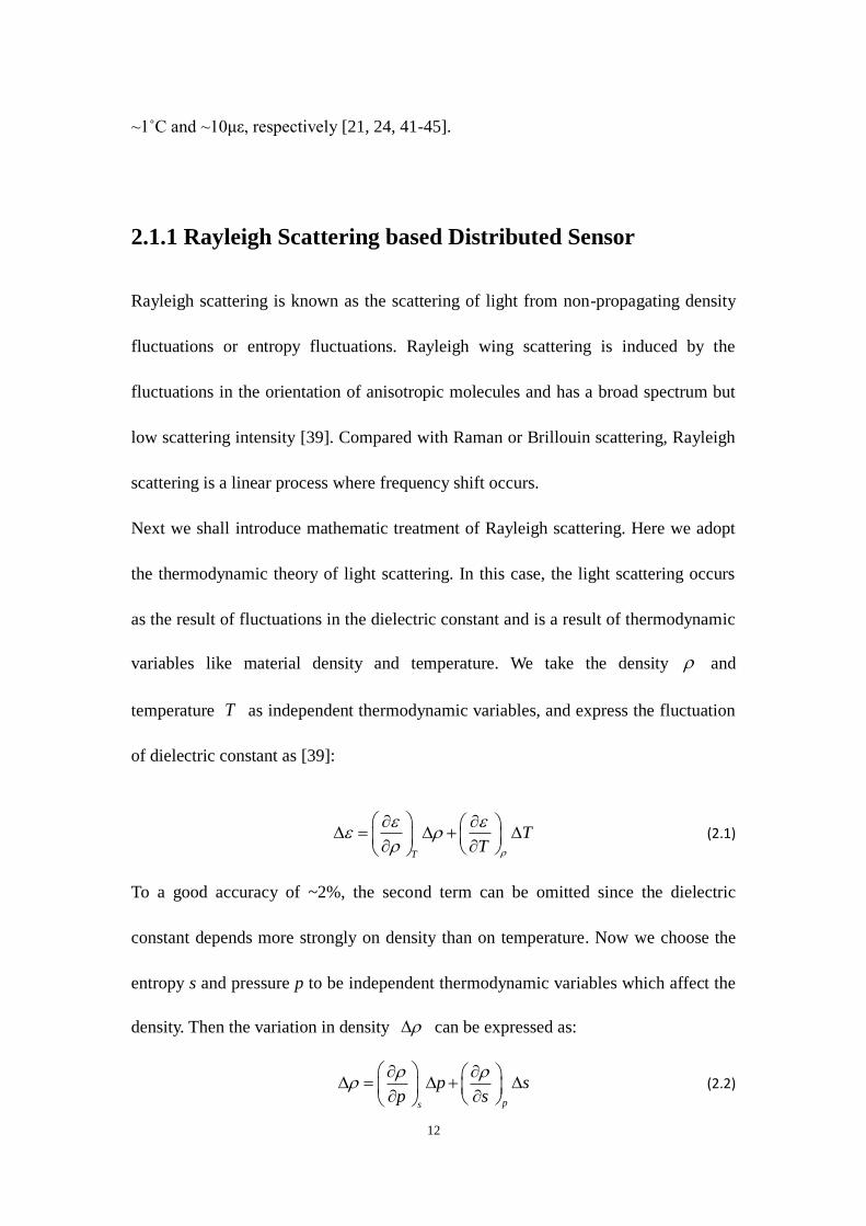
For silica, 113mW / cm K , 2.648g / cm ,
pc 0.7J / gK , taking all these
parameters into account, a typical value of FWHM of Rayleigh backscattering light is
0.79MHz at 1550nm.
Over the last 20 years, Rayleigh backscattering based sensing has been proposed in 3
types [1], including optical time domain reflectometry (OTDR), optical low coherence
reflectometry (OLCR) and optical frequency domain reflectometry (OFDR).
2.1.2 Optical Time Domain Reflectometry (OTDR)
OTDR [40] is the most commonly used distributed sensing means and has had a long
history. Rayleigh OTDR is basically sending a pulsed laser into fiber under test and
measures the backscattering Rayleigh reflection or Fresnel reflection using a photo
detector (PD). After sending a series of pulses and averaging, the spatial information
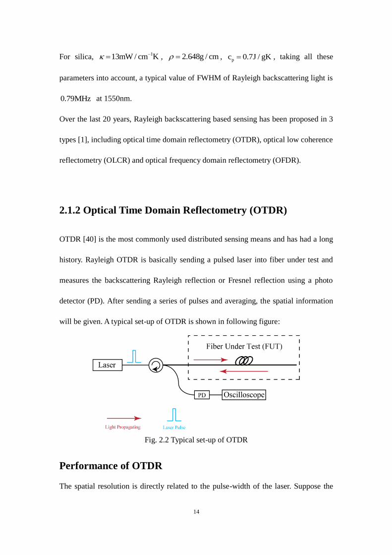
will be given. A typical set-up of OTDR is shown in following figure:
Fig. 2.2 Typical set-up of OTDR
Performance of OTDR
The spatial resolution is directly related to the pulse-width of the laser. Suppose the
15
laser has a pulse-width of time then it is impossible to distinguish the event within
the pulse duration. This pulse duration corresponds to a spatial resolution
/ 2 gl v , where gv is the group velocity in the fiber and with a typical value of
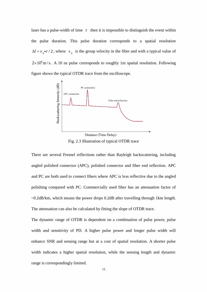
82 10 m / s . A 10 ns pulse corresponds to roughly 1m spatial resolution. Following
figure shows the typical OTDR trace from the oscilloscope.
Fig. 2.3 Illustration of typical OTDR trace
There are several Fresnel reflections rather than Rayleigh backscattering, including
angled polished connector (APC), polished connector and fiber end reflection. APC
and PC are both used to connect fibers where APC is less reflective due to the angled
polishing compared with PC. Commercially used fiber has an attenuation factor of
~0.2dB/km, which means the power drops 0.2dB after travelling through 1km length.
The attenuation can also be calculated by fitting the slope of OTDR trace.
The dynamic range of OTDR is dependent on a combination of pulse power, pulse
width and sensitivity of PD. A higher pulse power and longer pulse width will
enhance SNR and sensing range but at a cost of spatial resolution. A shorter pulse
width indicates a higher spatial resolution, while the sensing length and dynamic
range is correspondingly limited.
16
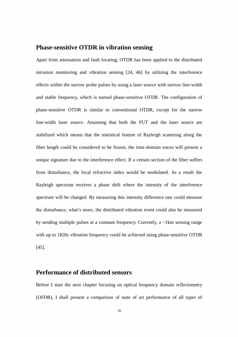
Phase-sensitive OTDR in vibration sensing
Apart from attenuation and fault locating, OTDR has been applied to the distributed
intrusion monitoring and vibration sensing [24, 46] by utilizing the interference
effects within the narrow probe pulses by using a laser source with narrow line-width
and stable frequency, which is named phase-sensitive OTDR. The configuration of
phase-sensitive OTDR is similar to conventional OTDR, except for the narrow
line-width laser source. Assuming that both the FUT and the laser source are
stabilized which means that the statistical feature of Rayleigh scattering along the
fiber length could be considered to be frozen, the time-domain traces will present a
unique signature due to the interference effect. If a certain section of the fiber suffers
from disturbance, the local refractive index would be modulated. As a result the
Rayleigh spectrum receives a phase shift where the intensity of the interference
spectrum will be changed. By measuring this intensity difference one could measure
the disturbance; what’s more, the distributed vibration event could also be measured
by sending multiple pulses at a constant frequency. Currently, a ~1km sensing range
with up to 1KHz vibration frequency could be achieved using phase-sensitive OTDR
[45].
Performance of distributed sensors
Before I start the next chapter focusing on optical frequency domain reflectometry
(OFDR), I shall present a comparison of state of art performance of all types of
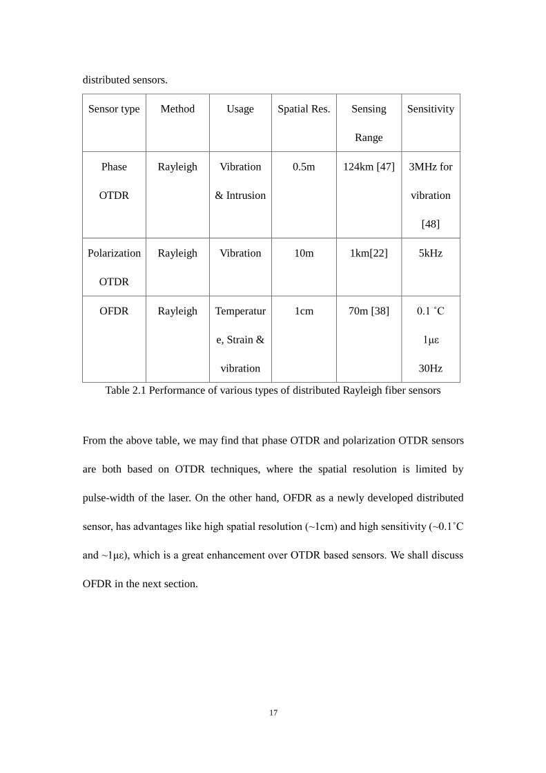
17
distributed sensors.
Sensor type Method Usage Spatial Res. Sensing
Range
Sensitivity
Phase
OTDR
Rayleigh Vibration
& Intrusion
0.5m 124km [47] 3MHz for
vibration
[48]
Polarization
OTDR
Rayleigh Vibration 10m 1km[22] 5kHz
OFDR Rayleigh Temperatur
e, Strain &
vibration
1cm 70m [38] 0.1 ˚C
1με
30Hz
Table 2.1 Performance of various types of distributed Rayleigh fiber sensors
From the above table, we may find that phase OTDR and polarization OTDR sensors
are both based on OTDR techniques, where the spatial resolution is limited by
pulse-width of the laser. On the other hand, OFDR as a newly developed distributed
sensor, has advantages like high spatial resolution (~1cm) and high sensitivity (~0.1˚C
and ~1με), which is a great enhancement over OTDR based sensors. We shall discuss
OFDR in the next section.
18
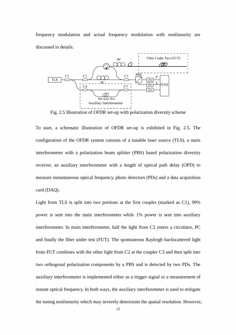
2.2 Theory of OFDR
2.2.1 Fundamental theory of OFDR with two electrical fields
In this section, a general set-up of OFDR is presented with the traditional set-up of
OFDR. To help understand the mechanism behind OFDR, a recapitulative theoretical
calculation with two electrical fields is provided [30].
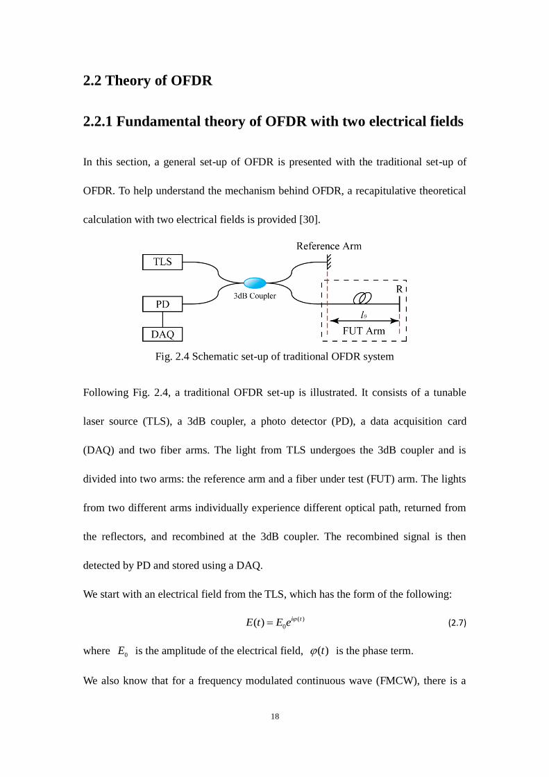
Fig. 2.4 Schematic set-up of traditional OFDR system
Following Fig. 2.4, a traditional OFDR set-up is illustrated. It consists of a tunable
laser source (TLS), a 3dB coupler, a photo detector (PD), a data acquisition card
(DAQ) and two fiber arms. The light from TLS undergoes the 3dB coupler and is
divided into two arms: the reference arm and a fiber under test (FUT) arm. The lights
from two different arms individually experience different optical path, returned from
the reflectors, and recombined at the 3dB coupler. The recombined signal is then
detected by PD and stored using a DAQ.
We start with an electrical field from the TLS, which has the form of the following:
( )
0( ) i tE t E e (2.7)
where 0E is the amplitude of the electrical field, ( )t is the phase term.
We also know that for a frequency modulated continuous wave (FMCW), there is a
19
relationship between modulated frequency and phase:
0
0
( ) ( )
t
t t dt (2.8)
For a single mode fiber, the chromatic dispersion for telecommunication optical
wavelength, which is 1550nm, is typically 20ps/(nm*km). Taking identical
wavelength sweeping range of 40nm and fiber length of 100m, the time delay induced
by chromatic dispersion equals 20 / ( ) 40 0.1 8ps nm km nm km ps , which
corresponds to a length of / 1.6delay efft c n mm . This is quite a small value compared
with the whole fiber length and thus the chromatic dispersion is negligible. To
simplify the calculation, the initial point is set at the output of the 3dB coupler; also
we ignore any attenuation effects in the fiber, where the electrical field at the
reference arm can be expressed as:
( )
1( ) i t
rE t E e (2.9)
The electrical field propagates and reflects at the mirror, and finally returned to the
output port with a 3dB coupler. If the distance between the output port and the mirror
is rl , which corresponds to a time delay of r , the electrical field can be expressed
as:
( 2 )
2( , ) ri t
r rE t E e
(2.10)
Similarly, the distance between the output port of 3dB coupler and a specific
reflection point in FUT arm can be notified as 0rl l , where rl is the same with the
one in reference arm, and 0l is the path difference between reference arm and FUT
arm. The electrical field of FUT can be then expressed as:
0( 2( ))
0 0( , ) ri t
FUT rE t E e
(2.11)
20
The electrical fields then combine at the coupler and being detected by the PD at the
other port. The electrical field at the detector can be expressed as:
0( 2( ))( 2 )
1 2
( ) ( ) ( )
rr
d r FUT
i ti t
E t E t E t
E e E e
(2.12)
The intensity of linearly polarized light can be represented as:
2 *( ) ( ) ( ) ( )d d dI t E t E t E t (2.13)
We then substitute Eq. (2.10) into Eq. (2.11), and the intensity can be expressed as:
* *
* * * *
1 2 0
0
( ) ( ( ) ( )) ( ( ) ( ))
( ) ( ) ( ) ( ) ( ) ( ) ( ) ( )
( ) ( ) 2 cos{ ( 2 ) ( 2( ))}
( ) ( ) 2 ( ) ( ) cos{ ( 2 ) ( 2( )
r FUT r FUT
r r FUT FUT r FUT FUT FUT
r FUT r r
r FUT r FUT r r
I t E t E t E t E t
E t E t E t E t E t E t E t E t
I t I t E E t t
I t I t I t I t t t
)}
(2.14)
Since the two electrical fields are from the same source, within the coherence length
the two electrical fields are correlated. Eq. (2.14) can be further simplified if we
introduce the visibility:
0 0( ) {1 cos{ ( 2 ) ( 2( ))}}r rI t I V t t (2.15)
here 2 / ( )r FUT r FUTV I I I I is the visibility of the interference pattern while
0 r FUTI I I . The visibility found its maximum value when r FUTI I .
If the wavelength is linearly tuned which is the case in OFDR system, as shown
below:
2
0 0 0
0 0
1( ) ( ) ( )
2
t t
t t dt t dt t t (2.16)
here 0( )t t is a linearly tuning frequency, the optical frequency tuning
speed, 0 the initial optical frequency. 0 is the initial phase from the TLS.
Then the interference term in Eq. (2.15) is reduced to:
0 0 0 0 0( ) {1 cos{ (2 2(2 )) 2 }}rI t I V t (2.17)
21
Note r is some time delay which has no contribution to the intensity, therefore can
be intentionally ignored. Finally the following formula can be obtained:
0 0 0 0 0 0( ) {1 cos{2 2 2 }}I t I V t (2.18)
From the above derivation, it is found that one specific location which has a distance
of 0l (and a time delay of 0 ) towards reference point corresponds to a beat
frequency of 02 . By performing an FFT, the beat frequency can be extracted and
viewed from the frequency spectrum. Therefore, OFDR system is able to monitor
reflection points within FUT and enjoys merits like high spatial resolution, quick
measurement and so on.
Please note that in the above derivation, only two electrical fields are calculated. This
is a good approximation for a strong reflection point in FUT, like PC connector or
mirror. However, in real OFDR measurement, the electrical field in ( )FUTE t is a
summation of all Rayleigh backscattering points within the fiber, thus cannot be
represented by the general idea above. This derivation did present general
understanding on how OFDR functions, however it is not rigorous to be a theoretical
derivation. In the following section, a detailed derivation treating multiple electrical
fields interference shall be given.
2.2.2 Fundamental Theory of OFDR with polarization
diversity scheme
In this section, the fundamental theory of OFDR shall be discussed with actual
experimental set-up and an analytical solution shall be given. Both ideal linear
22
frequency modulation and actual frequency modulation with nonlinearity are
discussed in details.
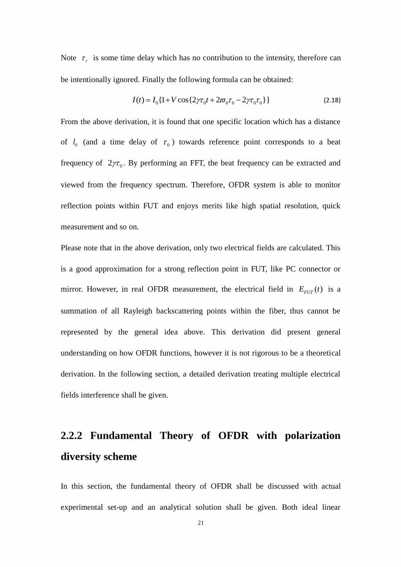
Fig. 2.5 Illustration of OFDR set-up with polarization diversity scheme
To start, a schematic illustration of OFDR set-up is exhibited in Fig. 2.5. The
configuration of the OFDR system consists of a tunable laser source (TLS), a main
interferometer with a polarization beam splitter (PBS) based polarization diversity
receiver, an auxiliary interferometer with a length of optical path delay (OPD) to
measure instantaneous optical frequency, photo detectors (PDs) and a data acquisition
card (DAQ).
Light from TLS is split into two portions at the first coupler (marked as C1), 99%
power is sent into the main interferometer while 1% power is sent into auxiliary
interferometer. In main interferometer, half the light from C2 enters a circulator, PC
and finally the fiber under test (FUT). The spontaneous Rayleigh backscattered light
from FUT combines with the other light from C2 at the coupler C3 and then split into
two orthogonal polarization components by a PBS and is detected by two PDs. The
auxiliary interferometer is implemented either as a trigger signal or a measurement of
instant optical frequency. In both ways, the auxiliary interferometer is used to mitigate
the tuning nonlinearity which may severely deteriorate the spatial resolution. However,
23
in this section we shall mainly focus on the mechanisms of OFDR, where an ideal
perfect linear tuning frequency is assumed, the compensation for tuning nonlinearity
shall be discussed in next section.
As shown in Fig. 2.5, the TLS has an optical frequency ( ) t and a phase of ( )t .
The light from coupler C2 is set as the zero point. The electrical field can be expresses
as [49]:
( )
0( ) ( ) i tE t E t e (2.19)
where 0 ( )E t is the amplitude of the electrical field.
If the light propagates a distance of l , the electrical field can be written as:
( )
0( , ) ( )2
i t lAE t E t e e (2.20)
where is the time delay and is proportional to l : / / ( / )gl V l c n , V is the
group velocity and gn is the group refractive index. A is a complex number
describing phase shift that undergoes a coupler or a circulator, is the attenuation
coefficient.
The electrical field at one arm of the main interferometer can be then expressed as
follows:
( )
0( , ) ( )2
b bi t lbb b
AE t E t e e
(2.21)
where b corresponds to time delay from C2 to C3, bl corresponds to the distance
from C2 to C3.
If we look at a specific position 'z at FUT, where a spontaneous Rayleigh
backscattering light is generated and undergoes the circulator and finally reaches the
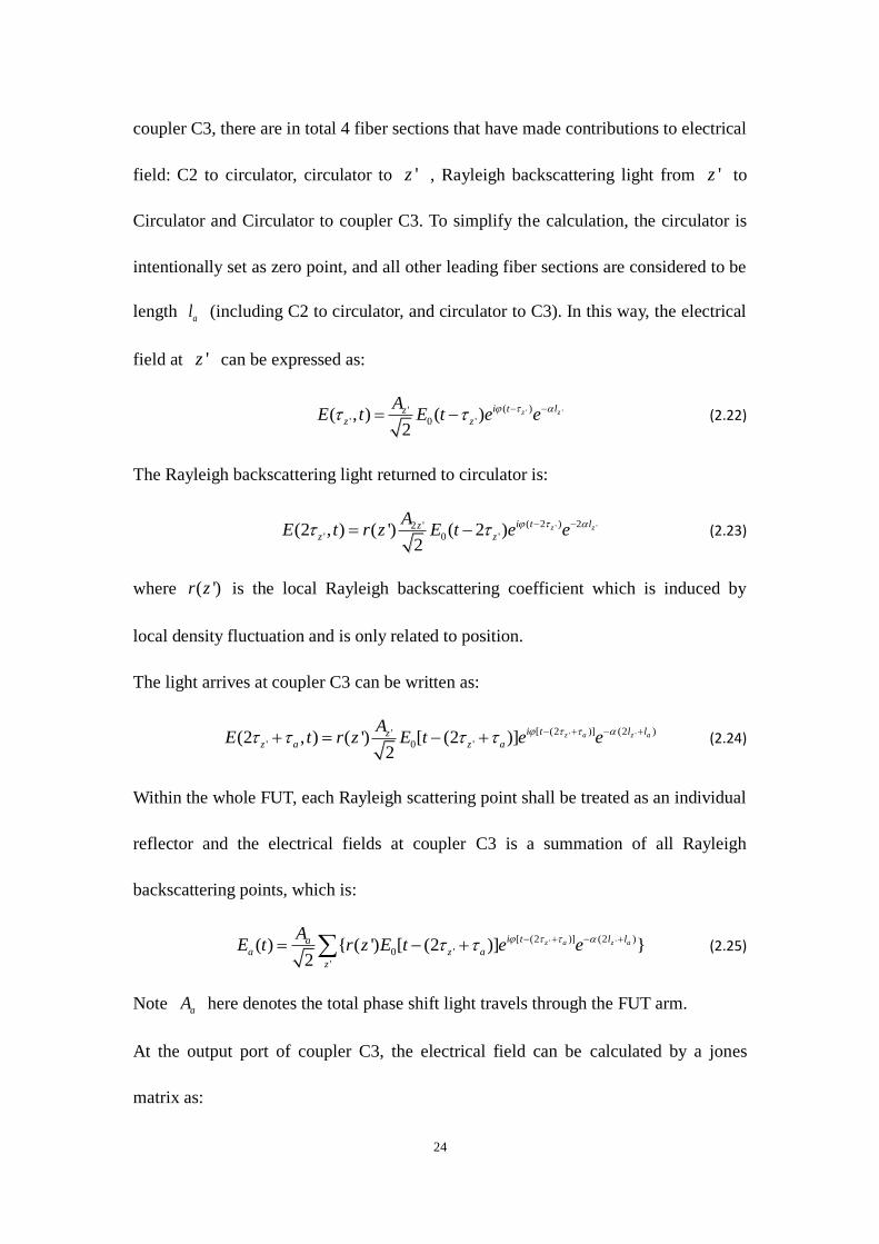
24
coupler C3, there are in total 4 fiber sections that have made contributions to electrical
field: C2 to circulator, circulator to 'z , Rayleigh backscattering light from 'z to
Circulator and Circulator to coupler C3. To simplify the calculation, the circulator is
intentionally set as zero point, and all other leading fiber sections are considered to be
length al (including C2 to circulator, and circulator to C3). In this way, the electrical
field at 'z can be expressed as:
' '( )'' 0 '( , ) ( )
2
z zi t lzz z
AE t E t e e
(2.22)
The Rayleigh backscattering light returned to circulator is:
' '( 2 ) 22 '' 0 '(2 , ) ( ') ( 2 )
2
z zi t lzz z
AE t r z E t e e
(2.23)
where ( ')r z is the local Rayleigh backscattering coefficient which is induced by
local density fluctuation and is only related to position.
The light arrives at coupler C3 can be written as:
' '[ (2 )] (2 )'' 0 '(2 , ) ( ') [ (2 )]
2
z a z ai t l lzz a z a
AE t r z E t e e
(2.24)
Within the whole FUT, each Rayleigh scattering point shall be treated as an individual
reflector and the electrical fields at coupler C3 is a summation of all Rayleigh
backscattering points, which is:
' '[ (2 )] (2 )
0 '
'
( ) { ( ') [ (2 )] }2
z a z ai t l laa z a
z
AE t r z E t e e
(2.25)
Note aA here denotes the total phase shift light travels through the FUT arm.
At the output port of coupler C3, the electrical field can be calculated by a jones
matrix as:
25
' '[ (2 )] (2 )
0 '
'
( )
0
( ) ( ) ( )
{ ( ') [ (2 )] }2
( )2
z a z a
b b
a b
i t l laz a
z
i t lbb
E t E t iE t
Ar z E t e e
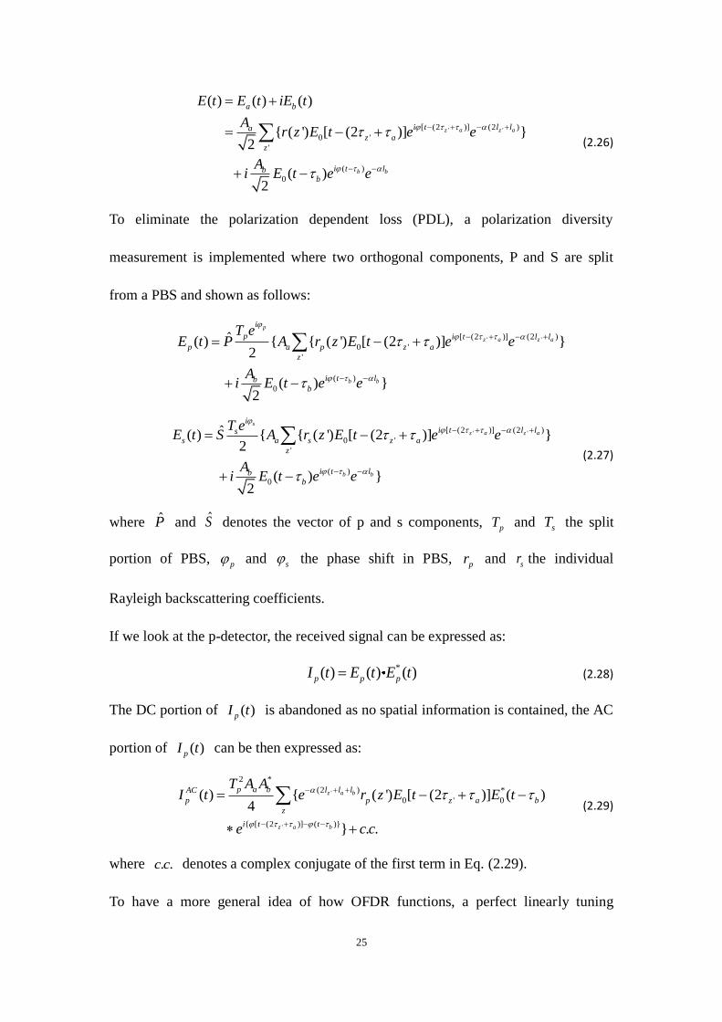
Ai E t e e
(2.26)
To eliminate the polarization dependent loss (PDL), a polarization diversity
measurement is implemented where two orthogonal components, P and S are split
from a PBS and shown as follows:
' '[ (2 )] (2 )
0 '
'
( )
0
ˆ( ) { { ( ') [ (2 )] }2
( ) }2
p
z a z a
b b
i
p i t l l
p a p z a
z
i t lbb
T eE t P A r z E t e e
Ai E t e e
' '[ (2 )] (2 )
0 '
'
( )
0
ˆ( ) { { ( ') [ (2 )] }2
( ) }2
s
z a z a
b b
ii t l ls
s a s z a
z
i t lbb
T eE t S A r z E t e e
Ai E t e e
(2.27)
where P and S denotes the vector of p and s components, pT and sT the split
portion of PBS, p and s the phase shift in PBS,
pr and sr the individual
Rayleigh backscattering coefficients.
If we look at the p-detector, the received signal can be expressed as:
*( ) ( ) ( )p p pI t E t E t (2.28)
The DC portion of ( )pI t is abandoned as no spatial information is contained, the AC
portion of ( )pI t can be then expressed as:
'
'
2 *
(2 ) *
0 ' 0
{ [ (2 )] ( )}
( ) { ( ') [ (2 )] ( )4
} . .
z a b
z a b
p a b l l lAC
p p z a b
z
i t t
T A AI t e r z E t E t
e c c
(2.29)
where . .c c denotes a complex conjugate of the first term in Eq. (2.29).
To have a more general idea of how OFDR functions, a perfect linearly tuning
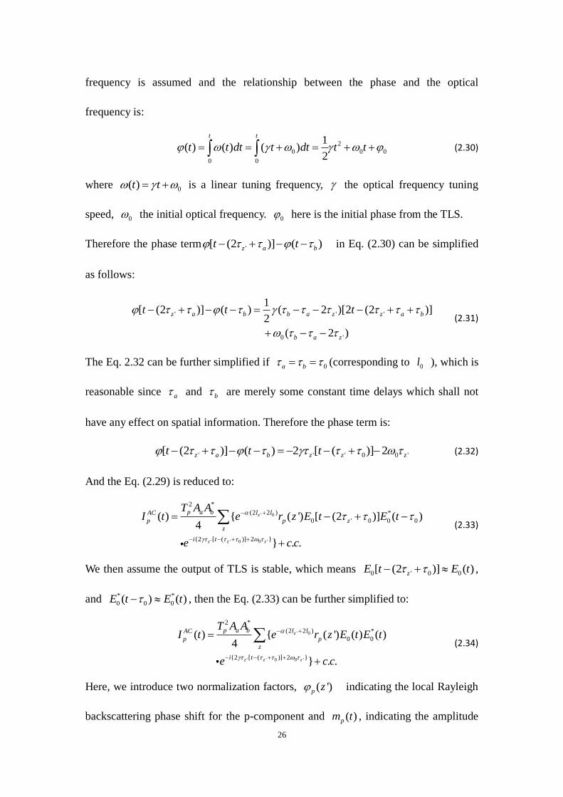
26
frequency is assumed and the relationship between the phase and the optical
frequency is:
2
0 0 0
0 0
1( ) ( ) ( )
2
t t
t t dt t dt t t (2.30)
where 0( )t t is a linear tuning frequency, the optical frequency tuning
speed, 0 the initial optical frequency. 0 here is the initial phase from the TLS.
Therefore the phase term '[ (2 )] ( )z a bt t in Eq. (2.30) can be simplified
as follows:
' ' '
0 '
1[ (2 )] ( ) ( 2 )[2 (2 )]
2
( 2 )
z a b b a z z a b
b a z
t t t
(2.31)
The Eq. 2.32 can be further simplified if 0a b (corresponding to 0l ), which is
reasonable since a and b are merely some constant time delays which shall not
have any effect on spatial information. Therefore the phase term is:
' ' ' 0 0 '[ (2 )] ( ) 2 [ ( )] 2z a b z z zt t t (2.32)
And the Eq. (2.29) is reduced to:
' 0
' ' 0 0 '
2 *
(2 2 ) *
0 ' 0 0 0
{2 [ ( )] 2 }
( ) { ( ') [ (2 )] ( )4
} . .
z
z z z
p a b l lAC
p p z
z
i t
T A AI t e r z E t E t
e c c
(2.33)
We then assume the output of TLS is stable, which means 0 ' 0 0[ (2 )] ( )zE t E t ,
and * *
0 0 0( ) ( )E t E t , then the Eq. (2.33) can be further simplified to:
' 0
' ' 0 0 '
2 *
(2 2 ) *
0 0
{2 [ ( )] 2 }
( ) { ( ') ( ) ( )4
} . .
z
z z z
p a b l lAC
p p
z
i t
T A AI t e r z E t E t
e c c
(2.34)
Here, we introduce two normalization factors, ( ')p z indicating the local Rayleigh
backscattering phase shift for the p-component and ( )pm t , indicating the amplitude
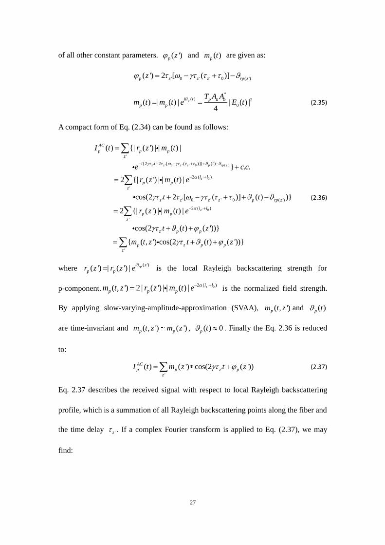
27
of all other constant parameters. ( ')p z and ( )pm t are given as:
' 0 ' ' 0 ( ')( ') 2 [ ( )]p z z z rp zz
*
( ) 2
0( ) | ( ) | | ( ) |4
pi t p a b
p p
T A Am t m t e E t
(2.35)
A compact form of Eq. (2.34) can be found as follows:
' ' 0 ' ' 0 ( ')
' 0
' 0
'
{2 2 [ ( )]} ( )
2 ( )
'
' ' 0 ' ' 0 ( ')
2 ( )
'
( ) {| ( ') | | ( ) |
} . .
2 {| ( ') | | ( ) |
cos(2 2 [ ( )] ( ) )}
2 {| ( ') | | ( ) |
z z z z p rp z
z
z
AC
p p p
z
i t t
l l
p p
z
z z z z p rp z
l l
p p
z
I t r z m t
e c c
r z m t e
t t
r z m t e
'
'
'
cos(2 ( ) ( '))}
{ ( , ') cos(2 ( ) ( '))}
z p p
p z p p
z
t t z
m t z t t z
(2.36)
where ( ')
( ') | ( ') | rpi z
p pr z r z e
is the local Rayleigh backscattering strength for
p-component. ' 02 ( )( , ') 2 | ( ') | | ( ) | zl l
p p pm t z r z m t e
is the normalized field strength.
By applying slow-varying-amplitude-approximation (SVAA), ( , ')pm t z and ( )p t
are time-invariant and ( , ') ( ')p pm t z m z , ( ) 0p t . Finally the Eq. 2.36 is reduced
to:
'
'
( ) ( ') cos(2 ( '))AC
p p z p
z
I t m z t z (2.37)
Eq. 2.37 describes the received signal with respect to local Rayleigh backscattering
profile, which is a summation of all Rayleigh backscattering points along the fiber and
the time delay 'z . If a complex Fourier transform is applied to Eq. (2.37), we may
find:
28
( ') ( ')
' '
'
( ) ( ( ))
2( ') ( 2 ) ( 2 )
2
p p
AC AC
p p
i z i z
p z z
z
I F I t
m z e e
(2.38)
Since 0 , the second term in Eq. 2.38 is neglected and an intuitive form of
distributed Rayleigh backscattering profile is provided:
( ')
'
'
'
'
2( ) ( ') ( 2 )
2
( ') ( 2 )
pi zAC
p p z
z
p z
z
I m z e
z
(2.39)
where ( ')2
( ') ( ')2
pi z
p pz m z e
is a coefficient and is only related to local
Rayleigh backscattering strength. '( 2 )z is an impulse function which
indicates a specific frequency (beat frequency) directly related to a position along the
fiber. By analyzing the frequency, the local scattering amplitude could be easily
observed.
The s-component from PBS could be derived similarly as well as the complex Fourier
transform. A polarization independent signal can be then obtained by adding p and s
components together which goes like follows:
'
'
( ) ( ') cos(2 ( '))AC
z
z
I t m z t z (2.40)
And in the frequency domain:
( ')
'
'
'
'
2( ) ( ') ( 2 )
2
( ') ( 2 )
AC i z
z
z
z
z
I m z e
z
(2.41)
From the above derivation, we theoretically analyzed the electrical field at PD and
through a Fourier transform, the frequency is found to be corresponding to local
position and the amplitude at which the frequency corresponds to the scattering
29
amplitude. Since a polarization diversity approach is implemented, the polarization
will have no effect on Rayleigh backscattering amplitude.
2.2.2.1 External Triggering in frequency domain treating
tuning nonlinearities
In the previous derivation, it is assumed that the tuning frequency is in a perfect linear
relationship with time, 0( )t t . However, this is not the case for any TLSs on
the market. Most TLSs employ a Fabry–Pérot (FP) etalon (or similar mode-selection
approaches), where the center wavelength is tuned by cavity length of the FP. The
cavity length can be either tuned by a DC motor for coarse-tuning or a piezoelectric
actuator for fine-tuning, but neither approach can provide linear tuning due to jitters in
mechanical parts, which may induce phase noise in lasing procedure. Luckily, some
previous work has been done by U. Glombitza and E. Brinkmeyer in their paper [49].
If we have a look at Eq. (2.41), where '
'
( ) ( ') ( 2 )AC
z
z
I z , one specific
frequency '2 z corresponds to a specific position 'z . The frequency tuning
speed ( )t is not a constant due to tuning nonlinearities, which means
'2 ( ) zt is not linear with 'z anymore.
If we recombine the electrical field, and expand it into Fourier series as follows:
0( ) ( )exp(2 )E t e i t d
(2.42)
where1 1
2 2
d
dt
is the instantaneous optical frequency. The light that
30
propagates to a specific position and then returns will induce a phase shift
'exp( ( )2 )zi l where ( ) is the propagation constant and z’ is the position of
Rayleigh scattering point. Combining them together, we may find:
0 '( ) ( )exp[ ( )2 ]exp(2 )zE t e i l i t d
(2.43)
The propagation constant can be approximated as 0 0 0( ) ( ) '( )( ) . The
first term 0( ) is related with phase delayph and second term 0'( ) is related
with group delay gr . With some procedures omitted, the beat signal can be
calculated as follows [49]:
2
0
1 0 0
{| | 2 | | cos( ( ) ( )1
2 ( ) )}
Neff n eff n gr
n ph gr
r r t tI I
(2.44)
here effr is some reflection factor. Remember ( ) ( ) / 2gr gr grt t d dt
where higher order terms are negligible. Substituting ( ) ( ) 2gr grt t into
above equation, a more simplified version can be found:
2
0 0
1
1 {| | 2 | | cos( 2 ')}N
eff n eff n gr
n
I I r r
(2.45)
where 0 0 0' 2 ( )ph gr is a summation of all constants. By taking the AC
portion of beat signal, finally the equation is reduced to:
0 0
1
2 | | cos( 2 ')N
eff n gr
n
I I r
(2.46)
From Eq. 2.46, we may find the time delay can be accurately measured whatever the
frequency tunes, provided the instantaneous optical frequency measured properly.
Each frequency corresponds to a specific gr . If the signal was sampled at even
time interval t , the frequency interval is not equal due to the tuning
31
nonlinearity. As a result, the spatial resolution will deteriorate to some extent,
depending on how nonlinear the tuning process is.
As previously stated, the equal frequency interval could provide accurate time
delay from FUT. One smart approach to achieve this is by employing an unbalanced
Mach-Zehnder interferometer (MZI) as an external trigger, which has been shown on
Fig. 2.5 as an auxiliary interferometer.
The analysis on auxiliary MZI is similar to that in main interferometer, two arms of
MZI undergo different optical paths and result in a time delay d :
( )
1 0
( )
2 0
( )
( ) d
i t
i t
E t E e
E t E e
(2.47)
The interference signal at the output of MZI is:
1 2 1 2( ( ) ( )) ( ( ) ( ))
cos( ( ) ( ))d
I E t E t E t E t
t t
(2.48)
Considering a non-perfect linear sweep, the frequency tuning speed is not a constant:
0
0 0
( ) ( ) ( ( ) )
t t
t t dt t t dt (2.49)
Therefore the interference signal is:
0 0
0
0
cos{ ( ( ) ) ( ( ) ( ) ) }
cos [( ( ) ( )] ( ) )]
t
d d
t
d d d
I t t dt t t dt
t t t t dt
(2.50)
Their first term [( ( ) ( )]dt t t is negligible since ( ) ( )dt t , and:
0
cos( ( ) )
t
dI t dt (2.51)
Since the auxiliary interferometer is employed as a rising-edge trigger, the
corresponding frequency interval is therefore a constant.
32
2.2.2.2 Laser Linewidth Effect on Sensing Range
As being derived from the following section 2.2.4.1, it is found that the maximum
sensing range is a quarter of the optical path difference from the auxiliary
interferometer. However, OPD cannot be infinitely extended as one must keep a high
contrast beat signal, which is then employed to trigger data acquisition in main
interferometer. In this case, laser linewidth plays a dominant role. Laser linewidth is
defined as the spectral linewidth of the laser, and is used to calculate coherent length.
If the OPD is close or beyond laser coherent length, the beat signal is averaged out
and the phase information to recover the instantaneous optical frequency deviates
from real value, which then leads to a high temperature and strain uncertainty; this is a
fundamental limit for triggered interferometer OFDR. Therefore, in triggered OFDR
configuration, the sensing range is in principle limited by the laser coherent length
with a maximum value of a quarter of laser coherent length. Typical OFDR products
on market only possess a sensing range of 70m [38]. However, the sensing range can
be ultimately close to coherence length, if it is not triggered by an auxiliary
interferometer, further details shall be discussed in Chapter 3.
33
2.2.3 Distributed Temperature and Strain sensing based on
OFDR
OFDR is primarily used to characterize and analyze network and optical waveguides
until 1998, where local Rayleigh profile is found to have similarities with fiber Bragg
gratings (FBG). This unique property is then employed in distributed temperature and
strain sensing. In this section, the principles of distributed temperature and strain
sensing based on local Rayleigh backscattering profile are discussed.
Weak FBG Model of OFDR
In previous sections, we have learned that the local Rayleigh backscattering profile
along the fiber is obtained through a fast Fourier transform (FFT) and could be
implemented in analyzing the optical networks, e.g. detecting fault position, where
usually large scattering amplitude exists. However, the Rayleigh backscattering
profile is also feasible for other applications since Rayleigh backscatter in optical
fiber is caused by random fluctuations in the index profile along the fiber length. For a
given fiber, the Rayleigh scattering amplitude as a function of distance is random but
static, thus can be modeled as a weak FBG with random period [50]. This “Rayleigh”
FBG is weak in amplitude but stable in different locations. To have a better
understanding on principles of OFDR sensing, firstly we may recall the formula
concerning central wavelength, or the Bragg wavelength of FBG [4]:
2B en (2.52)
where en is the effective refractive index (RI) in the fiber core and is the grating
34
period. The effective refractive index quantifies the velocity of propagating light as
compared to its velocity in vacuum. en not only depends on the optical wavelength,
but also depends on the specific optical mode that propagates. For a multimode fiber,
as thousands of modes propagate in the fiber, en is a summation of all weighted
modes with different effective RIs.
A FBG is sensitive to environmental variations like temperature and strain, the
relative Bragg wavelength shift of a FBG due to temperature or strain change is given
by [4]:
/ TC C T (2.53)
where C is some coefficient of strain, and T nC is the thermal coefficient.
TC consists of two terms: is the thermal-expansion coefficient, which is induced
by grating period change, n is the thermal-optic coefficient, which is induced by
the effective RI change. A simple explanation can be found by differentiating both
sides of Eq. (2.53), with respect to temperature T:
( ) 2{ ( ) ( )}B e eT n T n T (2.54)
Apparently ( )en T contributes to n and ( )T contributes to .
In the above discussions, it is found that the FBG spectral response is sensitive to
temperature and strain. The distributed Rayleigh backscattering presents some similar
properties: changes in refractive index or physical length shift the reflected spectrum
in frequency. The physical length (or average grating period of Rayleigh
backscattering profile) and refractive index of the fiber are intrinsically sensitive to
environmental perturbations like temperature and strain. It is even possible for sensing
35
humidity (provided the fiber coating is hydrophilic) and, electromagnetic fields [31].
The wavelength shift , or frequency shift , of the backscatter pattern due to a
temperature change, T , or strain along the fiber axis, , is identical to the
response of a fiber Bragg grating:
/ / TK T K (2.55)
here TK is a summation of thermal-expansion coefficient and thermal-optic
coefficient n , with typical values of 6 10.55 10 C and
6 16.1 10 C ,
respectively. For , if the fiber is coated with coating, is a summation of
weighted thermal-expansion coefficients of both bare fiber and coating materials
where is slightly larger than that of single mode fiber.
K is the strain coefficient and is a function of refractive index en , strain-optic
tensor, ijp , and Poisson’s ratio, . Typical values given for n , 12p , 11p and
for germanium-doped silica yield a value for K of 0.787.
Therefore, OFDR could perform as a distributed sensor in the entire fiber length by
simply calibrating the wavelength shift for both temperature and strain in a moderate
range (larger perturbations will induce slight nonlinearities as is wavelength
dependent).
2.2.4 Sensing resolution vs. spatial resolution
In the above section, the mechanism of OFDR sensing is reviewed. In this section we
shall introduce some further discussion on sensing length, spatial resolution, sensing
36
accuracy and sensing resolution.
2.2.4.1 Spatial Resolution
Firstly, we shall introduce the spatial resolution of OFDR system and a derivation
shall be given in later section. The spatial resolution z is determined by frequency
bandwidth of the scanning range from the following equation:
/ 2 gz c n (2.56)
Remember the optical frequency has the following relationship with optical
wavelength:
/c (2.57)
Differentiating both sides,
2/c (2.58)
And substitutes into Eq. 2.57, we got:
2 / 2 gz n (2.59)
The above Eq. (2.59) describes the relationship between spatial resolution z ,
central wavelength , and wavelength tuning range . Given a fixed central
wavelength, the larger wavelength tuning range corresponds to a higher spatial
resolution.
Beat Frequency (Sampling Frequency)
By employing the auxiliary interferometer, a constant frequency interval sampling is
guaranteed. Suppose the length difference of the two arms in the auxiliary
interferometer is l , which corresponds to a time delay of / /g gl v n l c . Also the
optical frequency delay between two arms can be found as ( / )d dt .
37
Converting the units into Hz, the beat frequency is expressed as:
2
2
2 ( / )/ 2
2 2
( / )
g g g
beat
g
n l n l n ld d c t
c dt c dt c
tn l
(2.60)
here / t represents an average wavelength tuning speed. beat also represents
the data sampling rate. Taking typical values, wavelength tuning range 40nm ,
wavelength tuning time 1t s , group RI 1.45gn ,a length difference 200l m
and a central wavelength of 1550nm , one may find 4.83beat MHz . This value
is of significance as it provides the minimum sampling speed of the DAQ. In fact,
beat is not constant within the whole tuning process, as a result the sampling rate of
DAQ often doubles (~10MHz).
Total Samples
Total samples taken in tuning process are acquired by multiplying beat and sampling
time samplingT , as follows:
2total beat sampling gS T n l
(2.61)
Typically, if 1samplingT s , which means TLS sweeps a 40nm wavelength range in 1s,
the total samples taken equals 4.83 Mega samples.
When performing an FFT, samplingT reduces to a half due to Nyquist–Shannon
sampling theorem:
22
g
FFT
n lS
(2.62)
Since the maximum sensing length 1
4FUT auxiliaryl l :
38
2 2
4 2
2
g FUT g FUT
FFT
n l n lS
(2.63)
Therefore, the number of points per meter is simply /FFT FUTS l :
/ 2
2/
g
P m FFT FUT
nS S l
(2.64)
Taking the above parameters, we get / 48.3 /P mS k points m , thus corresponds to a
spatial resolution of 2 / 2 20.7gz n m , which is exactly the Eq. (2.59).
2.2.4.2 Sensing Resolution vs Spatial Resolution
To define the sensing resolution, one must determine the maximum error in the
wavelength shift in performing cross-correlation. The peak wavelength shift by
performing a cross-correlation is ideally zero if no environmental disturbance occurs,
which indicates an extremely high precision. However, this is not the case in OFDR
as only a small portion of spatial points is used to do the cross-correlation. Clearly, a
larger number of data will reduce the uncertainty of the wavelength shift but at a cost
of lower spatial resolution [35]. Therefore, it is a trade-off between the sensing
resolution and spatial resolution. Previous work has been done by Xiaozhen Wang. et,
al. [35], where 100 times OFDR measurements were individually performed without
disturbance. Then the cross-correlation was calculated and the wavelength shift was
measured as a function of number of data. It is found that the uncertainty is as high as
~17pm at 1mm (80 data points) spatial resolution, while it decreases to ~4pm at
3.85mm (300 data points) spatial resolution. Using the typical temperature response,
39
the accuracy is found to be 1.7 C and 0.4 C , respectively. For typical OFDR
application with 40nm wavelength tuning range, 1cm spatial resolution commonly
corresponds to ~ 0.1 C temperature resolution, which is the best performance in all
kinds of distributed fiber sensors.
In summary, the spatial resolution of OFDR system was theoretically analyzed in this
chapter, while the sensing resolution is also determined by calculating the uncertainty
of the wavelength shift. To guarantee a certain level of sensing resolution, a number
of data points have to be taken in cross-correlation which therefore result in a
trade-off between spatial resolution and sensing accuracy.
40
Chapter 3
Extended sensing length of OFDR
3.1 Introduction
In this chapter, several nonlinearity compensation algorithms are proposed and
experimentally demonstrated in purpose to extend the sensing length of conventional
nonlinear triggered OFDR. In conventional OFDR, an auxiliary interferometer (AI) is
employed to trigger data acquisition where an equal frequency interval is guaranteed.
However, there are two main drawbacks in using the AI: firstly, the maximum sensing
length is limited by the optical path difference (OPD) of AI, which is in fact only a
quarter of the OPD of AI in order to satisfy the Nyquist Sampling theorem. Secondly,
the OPD of AI must be much shorter than the laser coherent length to generate correct
trigger. Even OPD close to coherent length may introduce errors in the triggered
signals from the auxiliary interferometer where polarization mode dispersion and
phase noise exist. Considering both restrictions, the sensing range of conventional
nonlinear triggered OFDR is less than one quarter the coherent length of TLS. In fact,
the commercial OFDR system in market has a sensing length of only 70m [38].
As discussed above, the sensing length cannot exceed the coherence length of TLS.
However, it could be significantly extended (close to coherence length of TLS) if the
auxiliary interferometer is not employed, which requires some other techniques to
41
suppress the tuning nonlinearities. Several approaches have been proposed regarding
this issue: Firstly, one could use laser sources of linear frequency tuning within a
microwave frequency domain over a small tuning range by an electrical optical
modulator [51], however, small tuning range corresponds to poor sensing accuracy,
which limits its usage. Another method is to compensate the tuning nonlinearity of the
TLS frequency scanning afterwards, in other words to resample signals from OFDR
with an equal frequency interval where the optical frequency can be extracted from
the auxiliary interferometer [34, 50-60]. This is a promising approach to extend the
sensing length to as long as laser coherent length but previous works only focus on
fault locating rather than sensing.
In this chapter, we adopt 3 different data processing approaches, including
non-uniform fast Fourier transform (NU-FFT), Deskew filter and cubic spline
interpolation, to resample the data from OFDR. Resampling principles, performances
are discussed for each approach. The result indicates that, one of those algorithms --
cubic spline interpolation resamples data with high accuracy which is capable for
distributed temperature and strain sensing.
3.2 Frequency Tuning Nonlinearity Compensation by Using
Non-Uniform FFT (NUFFT)
I came to a variety of approaches in order to compensate the frequency tuning
nonlinearity in OFDR system where the Non-Uniform Fast Fourier Transform
42
(NU-FFT) is the first trial I made in order to realize data resampling. NU-FFT [57, 61,
62] is a resampling scheme that is well accepted for non-equal spaced sampling in
frequency domain, which has been applied in many applications like Magnetic
Resonance Imaging (MRI) [62], Optical Coherence Tomography [55, 63, 64], and
other applications.
3.2.1 Theory of NU-FFT
The basic principle of frequency tuning nonlinearity compensation using NU-FFT is
to resample the beat signal in the main interferometer where the nonlinear
instantaneous frequency was subtracted from an auxiliary interferometer. The
auxiliary interferometer consists of two couplers, where two sections of fibers are
connected with an OPD. Suppose the group delay difference of the two arms is ,
the interference signal can be expressed as [54],
( ) cos 2 ( )0
I t U v t (3.1)
Where U0 is the amplitude of the beat signal, and v(t) is the instantaneous optical
frequency of the tunable laser source (TLS), the DC term in I(t) is automatically
removed as the photo detector is AC coupled. To obtain the instantaneous optical
frequency v(t), a Hilbert transform can be applied to the interference signal, where an
/ 2 is added on phase term of I(t), and we can get,
( ) H ( ) cos 2 ( ) / 2 sin 2 ( )0 0HI t I t U v t U v t (3.2)
Finally, the instantaneous optical frequency is recovered as follows,
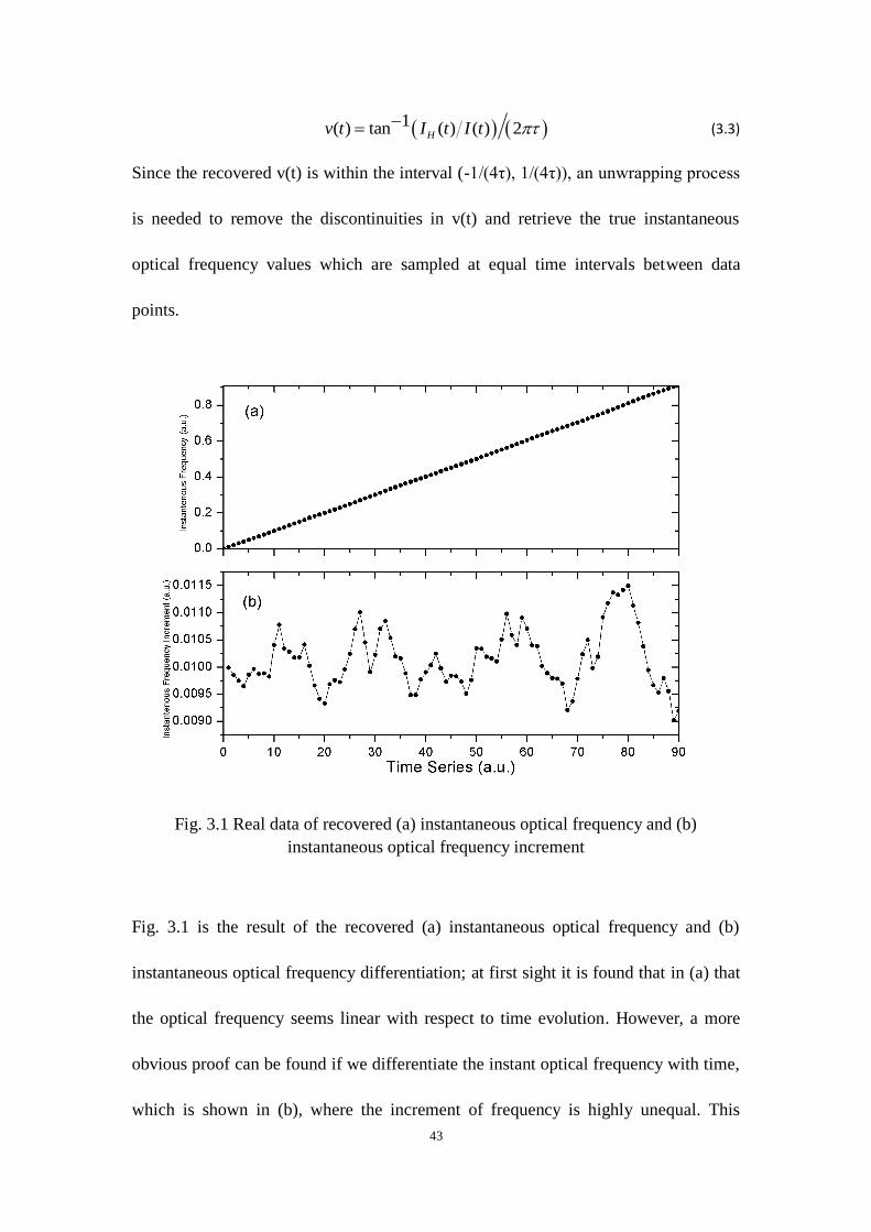
43
1( ) tan ( ) ( ) 2Hv t I t I t (3.3)
Since the recovered v(t) is within the interval (-1/(4τ), 1/(4τ)), an unwrapping process
is needed to remove the discontinuities in v(t) and retrieve the true instantaneous
optical frequency values which are sampled at equal time intervals between data
points.
Fig. 3.1 Real data of recovered (a) instantaneous optical frequency and (b)
instantaneous optical frequency increment
Fig. 3.1 is the result of the recovered (a) instantaneous optical frequency and (b)
instantaneous optical frequency differentiation; at first sight it is found that in (a) that
the optical frequency seems linear with respect to time evolution. However, a more
obvious proof can be found if we differentiate the instant optical frequency with time,
which is shown in (b), where the increment of frequency is highly unequal. This
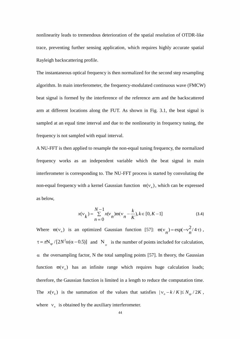
44
nonlinearity leads to tremendous deterioration of the spatial resolution of OTDR-like
trace, preventing further sensing application, which requires highly accurate spatial
Rayleigh backscattering profile.
The instantaneous optical frequency is then normalized for the second step resampling
algorithm. In main interferometer, the frequency-modulated continuous wave (FMCW)
beat signal is formed by the interference of the reference arm and the backscattered
arm at different locations along the FUT. As shown in Fig. 3.1, the beat signal is
sampled at an equal time interval and due to the nonlinearity in frequency tuning, the
frequency is not sampled with equal interval.
A NU-FFT is then applied to resample the non-equal tuning frequency, the normalized
frequency works as an independent variable which the beat signal in main
interferometer is corresponding to. The NU-FFT process is started by convoluting the
non-equal frequency with a kernel Gaussian function ( )n , which can be expressed
as below,
1
( ) ( ) ), [0, 1]
0
N kx x k K
k n n Kn
(3.4)
Where )n is an optimized Gaussian function [57]: 2) exp( / 4n n
,
2/ [2 0.5)]sp N and sp
is the number of points included for calculation,
the oversampling factor, N the total sampling points [57]. In theory, the Gaussian
function )n has an infinite range which requires huge calculation loads;
therefore, the Gaussian function is limited in a length to reduce the computation time.
The ( )kx is the summation of the values that satisfies | / | / 2n spk K N K ,
where n is obtained by the auxiliary interferometer.
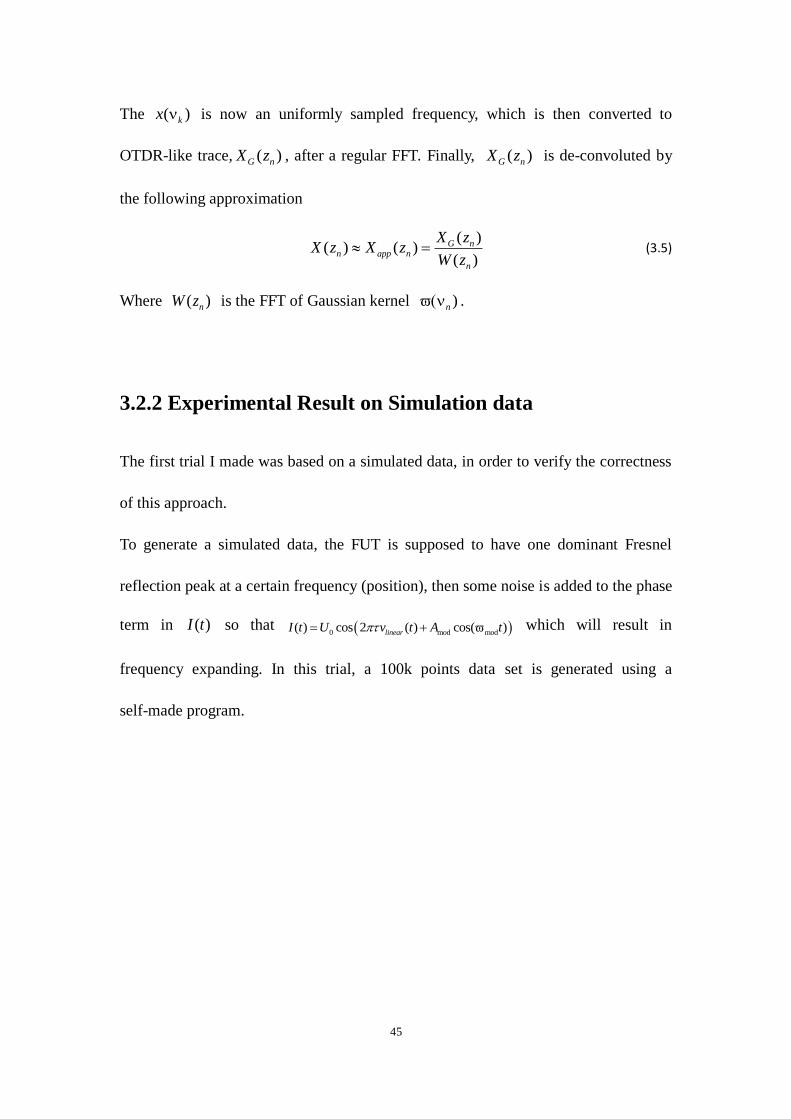
45
The ( )kx is now an uniformly sampled frequency, which is then converted to
OTDR-like trace, ( )G nX z , after a regular FFT. Finally, ( )G nX z is de-convoluted by
the following approximation
( )
( ) ( )( )
G nn app n
n
X zX z X z
W z (3.5)
Where ( )nW z is the FFT of Gaussian kernel )n .
3.2.2 Experimental Result on Simulation data
The first trial I made was based on a simulated data, in order to verify the correctness
of this approach.
To generate a simulated data, the FUT is supposed to have one dominant Fresnel
reflection peak at a certain frequency (position), then some noise is added to the phase
term in ( )I t so that 0 mod mod( ) cos 2 ( ) cos( )linearI t U v t A t which will result in
frequency expanding. In this trial, a 100k points data set is generated using a
self-made program.
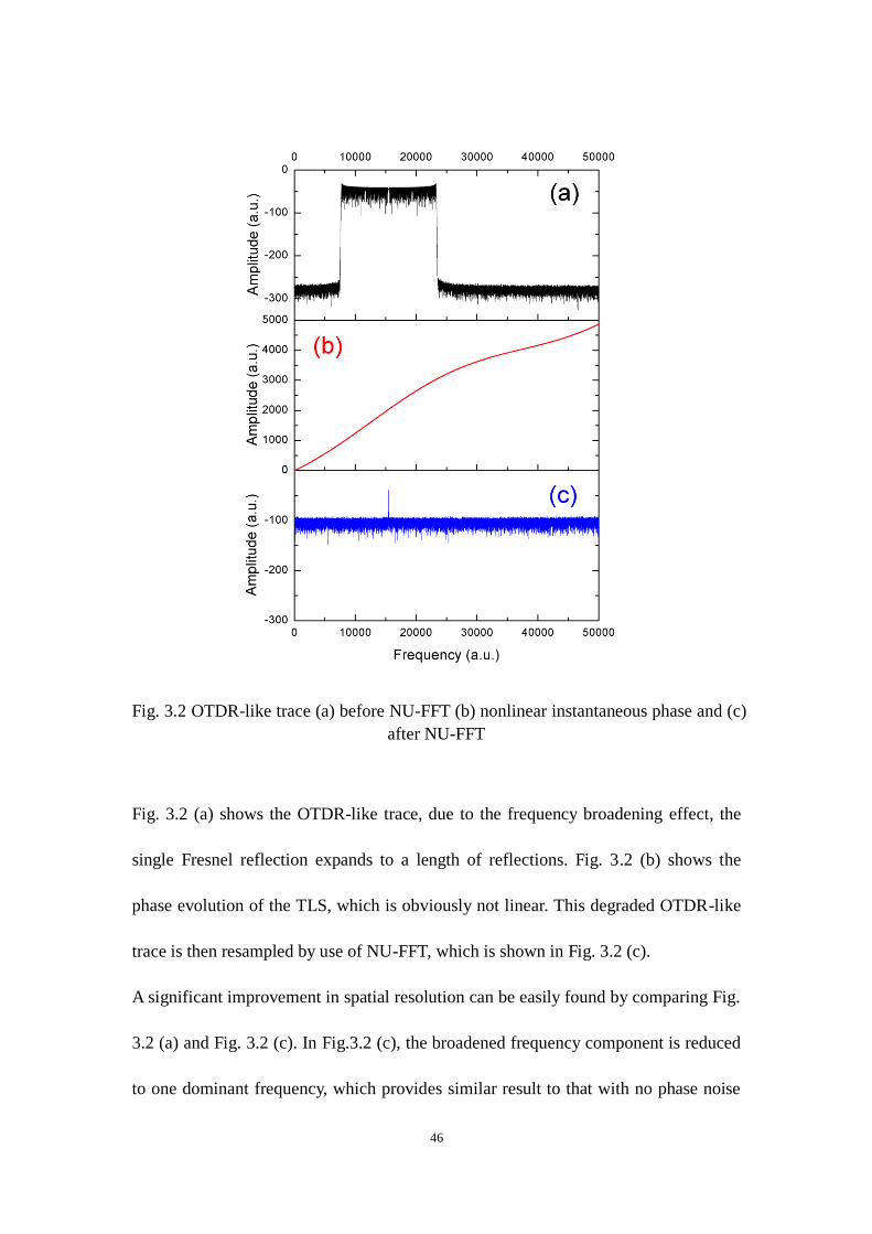
46
Fig. 3.2 OTDR-like trace (a) before NU-FFT (b) nonlinear instantaneous phase and (c)
after NU-FFT
Fig. 3.2 (a) shows the OTDR-like trace, due to the frequency broadening effect, the
single Fresnel reflection expands to a length of reflections. Fig. 3.2 (b) shows the
phase evolution of the TLS, which is obviously not linear. This degraded OTDR-like
trace is then resampled by use of NU-FFT, which is shown in Fig. 3.2 (c).
A significant improvement in spatial resolution can be easily found by comparing Fig.
3.2 (a) and Fig. 3.2 (c). In Fig.3.2 (c), the broadened frequency component is reduced
to one dominant frequency, which provides similar result to that with no phase noise
47
which verifies the correctness of this method. To make a more detailed comparison,
Fig. 3.2 (a) and Fig. 3.2 (c) are plotted with the same log scaling factors. We found
that the noise floor after the NU-FFT is about -100dB, while in Fig. 3.2 (a), the noise
floor of the deteriorated frequency data is -300dB which is much lower than the
compensated one. The increasing noise floor might decrease the Signal to Noise Ratio
(SNR), which is not beneficial to experiments. However, the compensated signal
keeps fairly high SNR which in my point of view might not affect the result.
3.2.3 Experimental Result on Real data
As NU-FFT is capable of resampling the simulated data, the next step is to examine
its actual performance on real data.
When it comes to real data, one thing that should be addressed is to guarantee that the
nonlinear phase is recovered correctly. In simulation data, the phase was intentionally
modified by a nonlinear term with slowly varying frequency and amplitude, which
makes the recovery of the phase easy. However, this is not the case in real data, as our
initial purpose is to make long range distributed sensing, which theoretically requires
large frequency sweeping range in order to achieve high temperature or strain
sensitivity. Given the maximum sampling rate and buffer of the data acquisition card
(DAQ), large frequency sweeping range requires fairly high frequency tuning speed,
which means only few points is within a 2 period in phase. In discrete signal
processing, the unwrapping phase progress commonly requires enough points within a
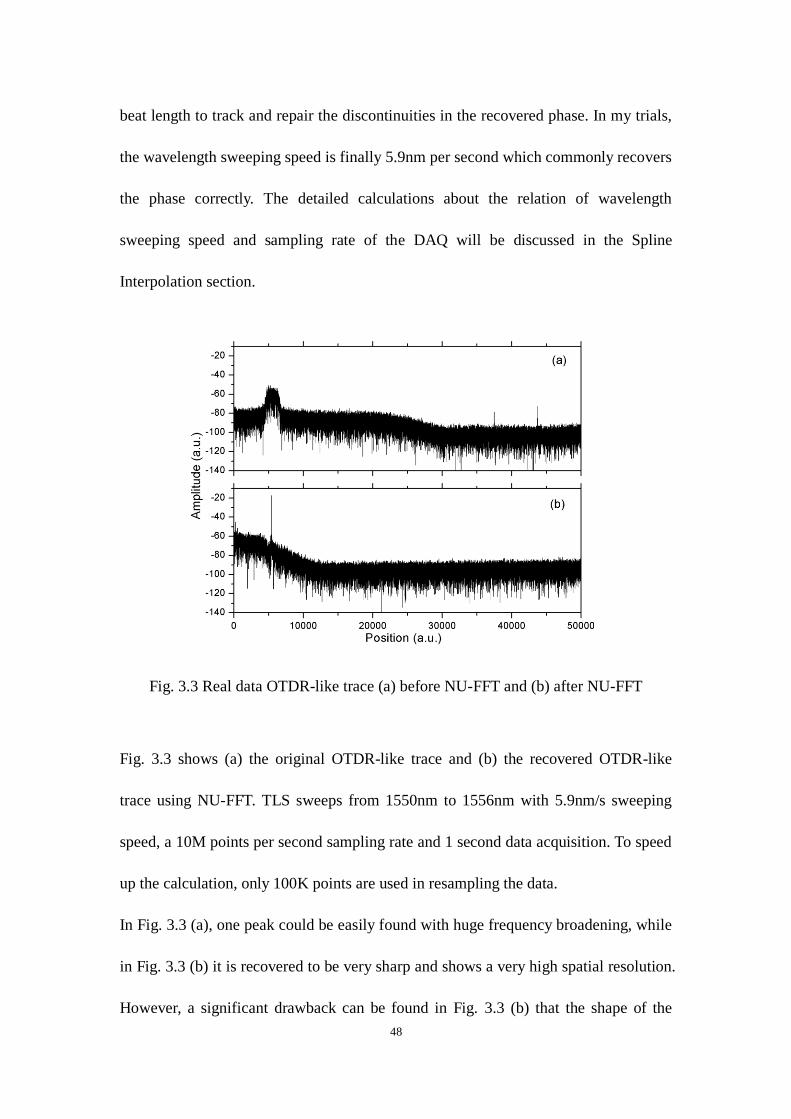
48
beat length to track and repair the discontinuities in the recovered phase. In my trials,
the wavelength sweeping speed is finally 5.9nm per second which commonly recovers
the phase correctly. The detailed calculations about the relation of wavelength
sweeping speed and sampling rate of the DAQ will be discussed in the Spline
Interpolation section.
Fig. 3.3 Real data OTDR-like trace (a) before NU-FFT and (b) after NU-FFT
Fig. 3.3 shows (a) the original OTDR-like trace and (b) the recovered OTDR-like
trace using NU-FFT. TLS sweeps from 1550nm to 1556nm with 5.9nm/s sweeping
speed, a 10M points per second sampling rate and 1 second data acquisition. To speed
up the calculation, only 100K points are used in resampling the data.
In Fig. 3.3 (a), one peak could be easily found with huge frequency broadening, while
in Fig. 3.3 (b) it is recovered to be very sharp and shows a very high spatial resolution.
However, a significant drawback can be found in Fig. 3.3 (b) that the shape of the
49
recovered signal is clearly a Gaussian instead of a commonly seen OTDR-like trace.
The reason shall be discussed in following section.
3.2.4 Limitations of NU-FFT
In Chap. 3.2.3, it is found that the recovered OTDR-like trace has a Gaussian shape
which tremendously reduces the sensing range. The reason to this drawback could be
explained as follows: the NU-FFT is actually an approach where the original raw data
( )nx convolutes with the Gaussian kernel function )n , according to
convolution:
( ( )* )) ( ) ( )n n n nF x k X z W z (3.6)
Where k is a constant that depends on the specific normalization of the Fourier
transform, ( )nX z is the FFT of ( )nx , and ( )nW z the FFT of )n , which
result in a Gaussian envelope in frequency spectrum and blurs the original flat
OTDR-like trace. By using the de-convolution approximation, this envelope can be
mitigated to some degree, however, at far frequency both the convoluted term
( )G nX z and FFT of Gaussian kernel ( )nW z are almost zero, as seen in Fig. 3.3 (b),
these two small decimals division would result in large error that in fact even larger
than error induced by nonlinearity itself, which limits the available length of NU-FFT
approach. By changing Gaussian kernel parameters like the over-sampling factor, the
Gaussian kernel leads to more broadening, which means longer sensing length can be
achieved, however, after all this NU-FFT cannot guarantee availability within the
50
whole range of the OTDR-like trace.
To make a summary, the NU-FFT approach to compensate for the nonlinearity in
OFDR is theoretically proven using a simulated broadened Fresnel reflection point
and experimentally demonstrated. The NU-FFT compensates the simulated data with
very good accuracy, however, when it comes to real data, NU-FFT is found to possess
a Gaussian envelope which blurs the OTDR-like trace that limits the total sensing
distance. As our final goal is to achieve long distance and high spatial resolution
OFDR sensing, the NU-FFT cannot satisfy all the requirements.
3.3 Frequency Tuning Nonlinearity Compensation by Using
Deskew Filter
As the NU-FFT approach cannot maintain OTDR-like trace within the whole sensing
length, one must find a new approach, which compensates the frequency tuning
nonlinearity without inducing new difficulties.
Considering the principles of OFDR is similar to that of frequency modulated radar in
radio frequency region, where some useful works have been done to reduce the tuning
nonlinearity in microwave band, my idea came to that maybe some algorithms could
be borrowed from radio frequency signal processing field. Luckily, some pioneering
works have been done, where Deskew filter is employed to reduce the degradation of
optical frequency tuning nonlinearity of the TLS in a long range [58]. The Deskew
filter is also known as Residual Video Phase (RVP) filter which originated from
51
Frequency Modulated Continuous Wave Synthetic Aperture Radar (FMCW SAR)
where frequency tuning or chirping nonlinearity also exists [65-67]. In theory, this
approach could eliminate all the tuning nonlinearity resulting from TLS if the
nonlinear phase could be predicted accurately. In [58] Ding proposed a 80km
distributed OFDR configuration with 20cm and 1.6m spatial resolution at distances of
10km and 80km, thus might become a powerful tool for long range distributed
temperature and strain sensing based on OFDR, where a large frequency tuning range
is required.
3.3.1 Theory of Deskew filter
As explained in previous chapter, the main interferometer in OFDR consists of two
arms, one named ( )sE t undergoes the fiber under test (FUT) while the other one
follows a reference path known as ( )rE t .
For TLS with a linear optical frequency tuning speed , the electrical field ( )rE t
could be written as,
2
0 0( ) exp{ [2 2 ( )]}rE t E j f t t e t (3.7)
Where 0f is the optical frequency, ( )e t the nonlinear phase term of TLS.
Assuming the reflection reflectivity at certain time delay is ( )r and the fiber
attenuation coefficient is , the signal ( )sE t could be written as,
2
0 0( ) ( ) exp{ [2 ( ) ( ) 2 ( )]}sE t R E j f t t e t (3.8)
Then at the coupler an AC coupled beat signal ( )I t interfered between local
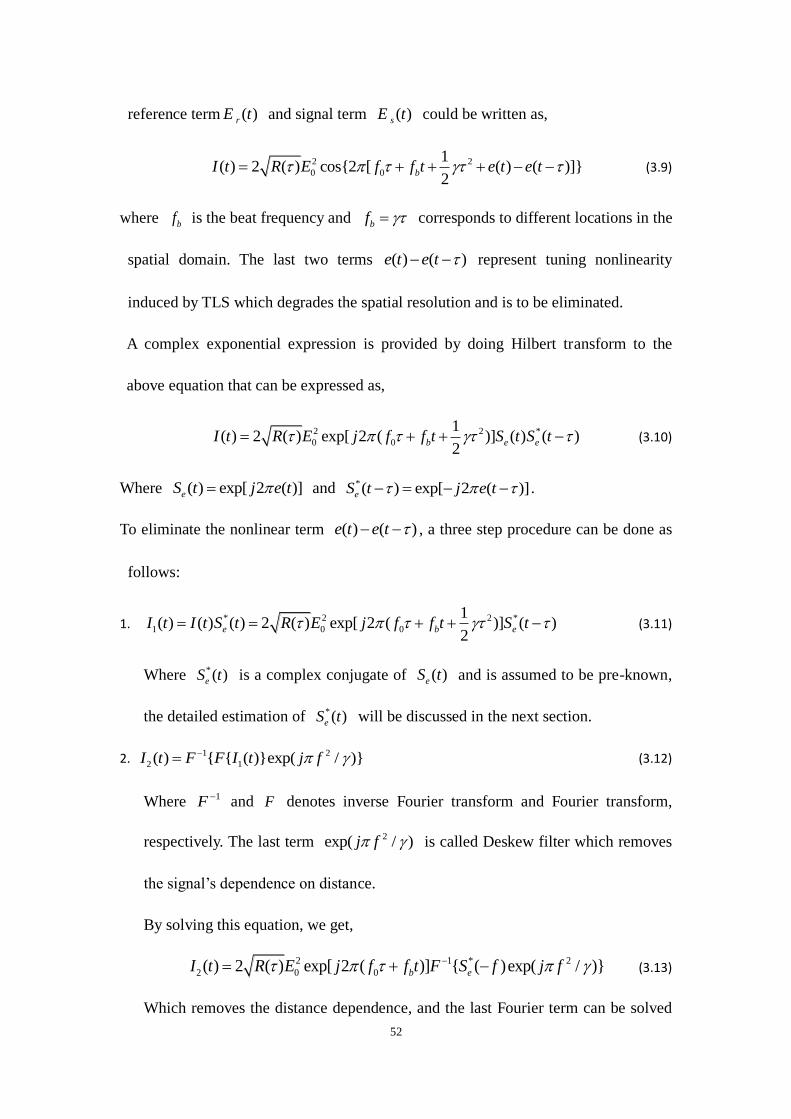
52
reference term ( )rE t and signal term ( )sE t could be written as,
2 2
0 0
1( ) 2 ( ) cos{2 [ ( ) ( )]}
2bI t R E f f t e t e t (3.9)
where bf is the beat frequency and bf corresponds to different locations in the
spatial domain. The last two terms ( ) ( )e t e t represent tuning nonlinearity
induced by TLS which degrades the spatial resolution and is to be eliminated.
A complex exponential expression is provided by doing Hilbert transform to the
above equation that can be expressed as,
2 2 *
0 0
1( ) 2 ( ) exp[ 2 ( )] ( ) ( )
2b e eI t R E j f f t S t S t (3.10)
Where ( ) exp[ 2 ( )]eS t j e t and *( ) exp[ 2 ( )]eS t j e t .
To eliminate the nonlinear term ( ) ( )e t e t , a three step procedure can be done as
follows:
1. * 2 2 *
1 0 0
1( ) ( ) ( ) 2 ( ) exp[ 2 ( )] ( )
2e b eI t I t S t R E j f f t S t (3.11)
Where *( )eS t is a complex conjugate of ( )eS t and is assumed to be pre-known,
the detailed estimation of *( )eS t will be discussed in the next section.
2. 1 2
2 1( ) { { ( )}exp( / )}I t F F I t j f (3.12)
Where 1F and F denotes inverse Fourier transform and Fourier transform,
respectively. The last term 2exp( / )j f is called Deskew filter which removes
the signal’s dependence on distance.
By solving this equation, we get,
2 1 * 2
2 0 0( ) 2 ( ) exp[ 2 ( )] { ( )exp( / )}b eI t R E j f f t F S f j f (3.13)
Which removes the distance dependence, and the last Fourier term can be solved
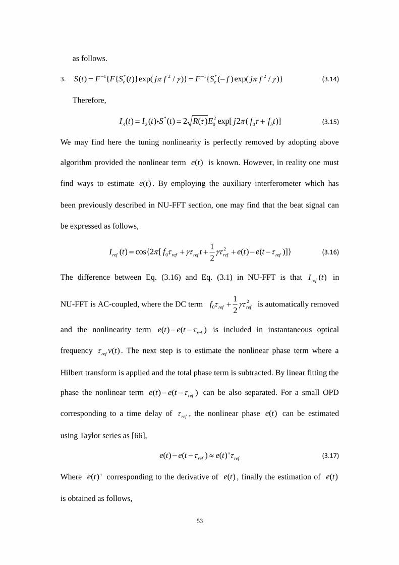
53
as follows.
3. 1 * 2 1 * 2( ) { { ( )}exp( / )} { ( )exp( / )}e eS t F F S t j f F S f j f (3.14)
Therefore,
* 2
3 2 0 0( ) ( ) ( ) 2 ( ) exp[ 2 ( )]bI t I t S t R E j f f t (3.15)
We may find here the tuning nonlinearity is perfectly removed by adopting above
algorithm provided the nonlinear term ( )e t is known. However, in reality one must
find ways to estimate ( )e t . By employing the auxiliary interferometer which has
been previously described in NU-FFT section, one may find that the beat signal can
be expressed as follows,
2
0
1( ) cos{2 [ ( ) ( )]}
2ref ref ref ref refI t f t e t e t (3.16)
The difference between Eq. (3.16) and Eq. (3.1) in NU-FFT is that ( )refI t in
NU-FFT is AC-coupled, where the DC term 2
0
1
2ref reff is automatically removed
and the nonlinearity term ( ) ( )refe t e t is included in instantaneous optical
frequency ( )ref v t . The next step is to estimate the nonlinear phase term where a
Hilbert transform is applied and the total phase term is subtracted. By linear fitting the
phase the nonlinear term ( ) ( )refe t e t can be also separated. For a small OPD
corresponding to a time delay of ref , the nonlinear phase ( )e t can be estimated
using Taylor series as [66],
( ) ( ) ( ) 'ref refe t e t e t (3.17)
Where ( ) 'e t corresponding to the derivative of ( )e t , finally the estimation of ( )e t
is obtained as follows,
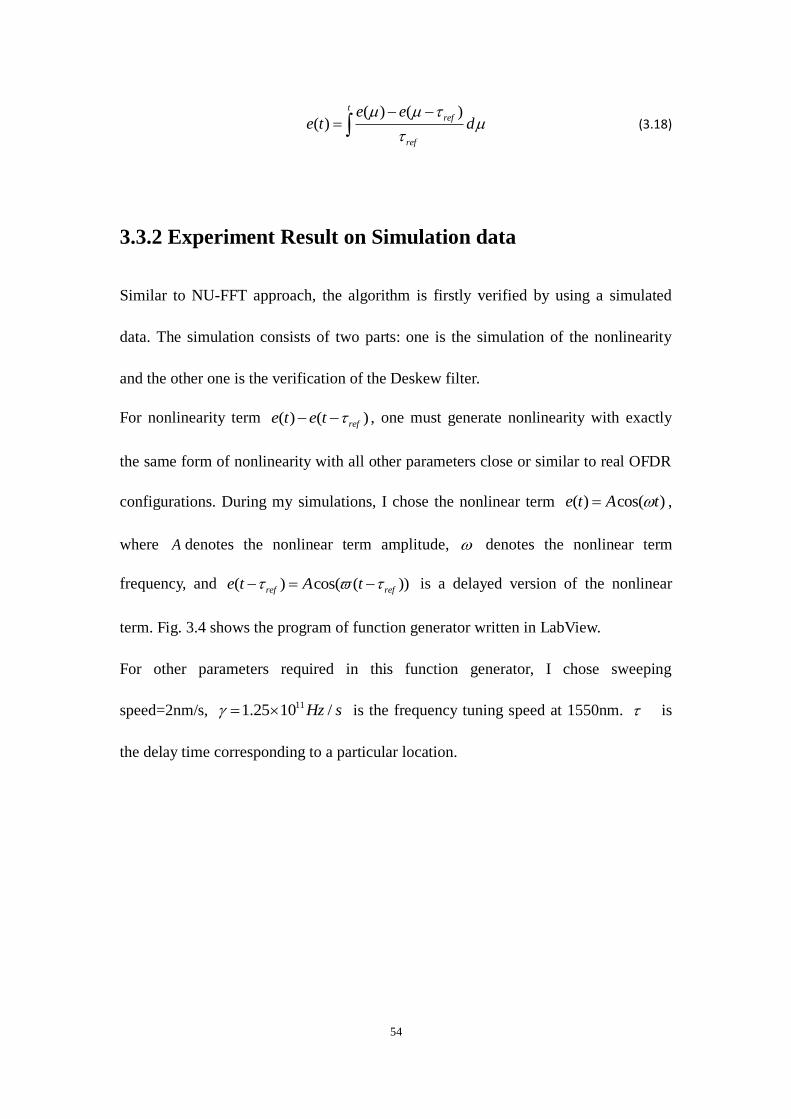
54
( ) ( )
( )
tref
ref
e ee t d
(3.18)
3.3.2 Experiment Result on Simulation data
Similar to NU-FFT approach, the algorithm is firstly verified by using a simulated
data. The simulation consists of two parts: one is the simulation of the nonlinearity
and the other one is the verification of the Deskew filter.
For nonlinearity term ( ) ( )refe t e t , one must generate nonlinearity with exactly
the same form of nonlinearity with all other parameters close or similar to real OFDR
configurations. During my simulations, I chose the nonlinear term ( ) cos( )e t A t ,
where A denotes the nonlinear term amplitude, denotes the nonlinear term
frequency, and ( ) cos( ( ))ref refe t A t is a delayed version of the nonlinear
term. Fig. 3.4 shows the program of function generator written in LabView.
For other parameters required in this function generator, I chose sweeping
speed=2nm/s, 111.25 10 /Hz s is the frequency tuning speed at 1550nm. is
the delay time corresponding to a particular location.
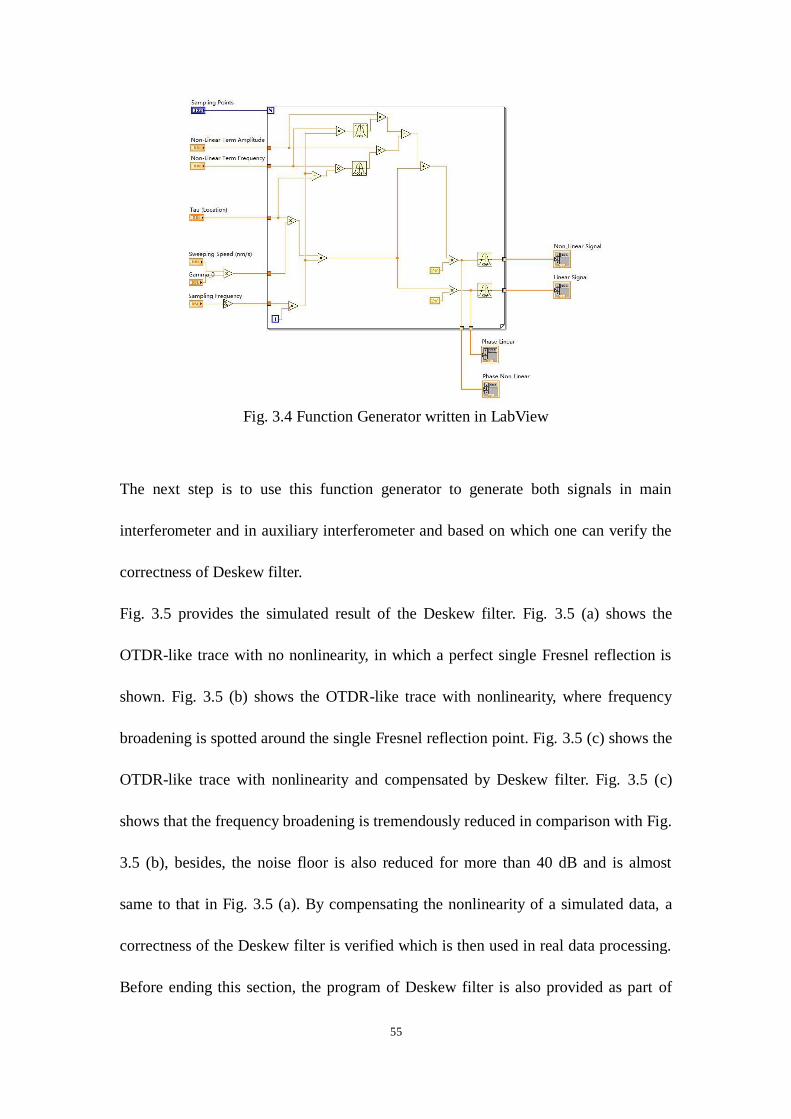
55
Fig. 3.4 Function Generator written in LabView
The next step is to use this function generator to generate both signals in main
interferometer and in auxiliary interferometer and based on which one can verify the
correctness of Deskew filter.
Fig. 3.5 provides the simulated result of the Deskew filter. Fig. 3.5 (a) shows the
OTDR-like trace with no nonlinearity, in which a perfect single Fresnel reflection is
shown. Fig. 3.5 (b) shows the OTDR-like trace with nonlinearity, where frequency
broadening is spotted around the single Fresnel reflection point. Fig. 3.5 (c) shows the
OTDR-like trace with nonlinearity and compensated by Deskew filter. Fig. 3.5 (c)
shows that the frequency broadening is tremendously reduced in comparison with Fig.
3.5 (b), besides, the noise floor is also reduced for more than 40 dB and is almost
same to that in Fig. 3.5 (a). By compensating the nonlinearity of a simulated data, a
correctness of the Deskew filter is verified which is then used in real data processing.
Before ending this section, the program of Deskew filter is also provided as part of
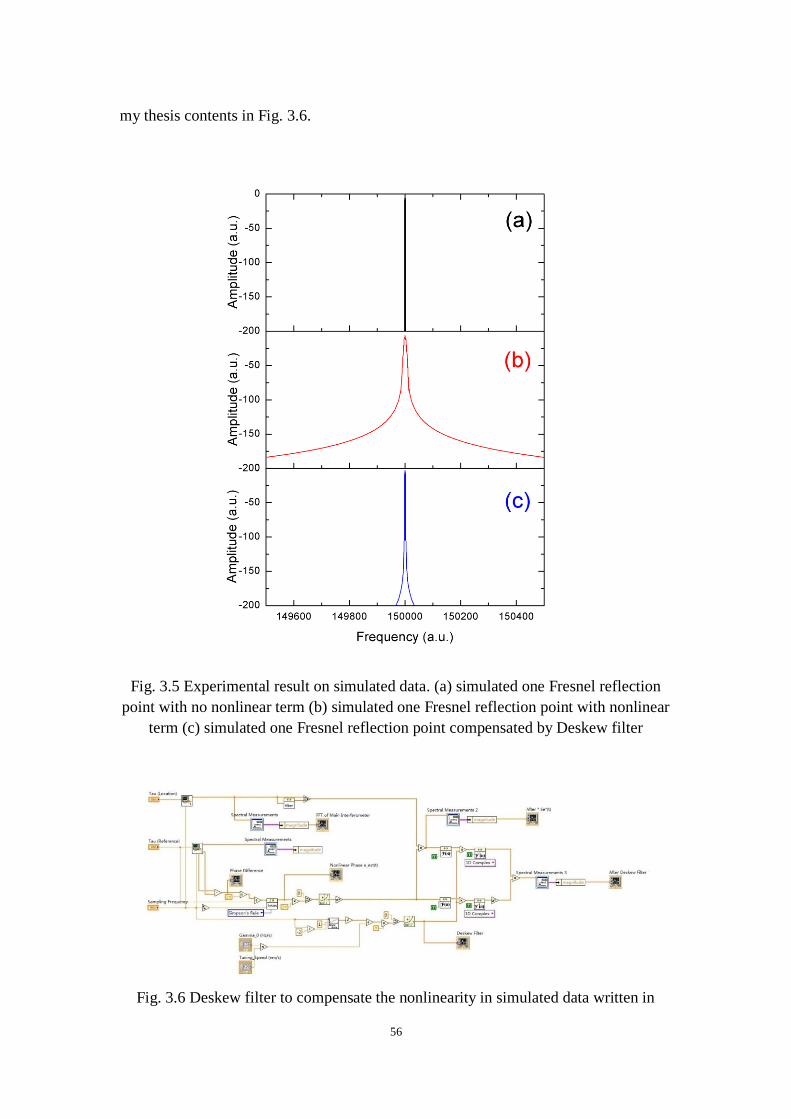
56
my thesis contents in Fig. 3.6.
Fig. 3.5 Experimental result on simulated data. (a) simulated one Fresnel reflection
point with no nonlinear term (b) simulated one Fresnel reflection point with nonlinear
term (c) simulated one Fresnel reflection point compensated by Deskew filter
Fig. 3.6 Deskew filter to compensate the nonlinearity in simulated data written in
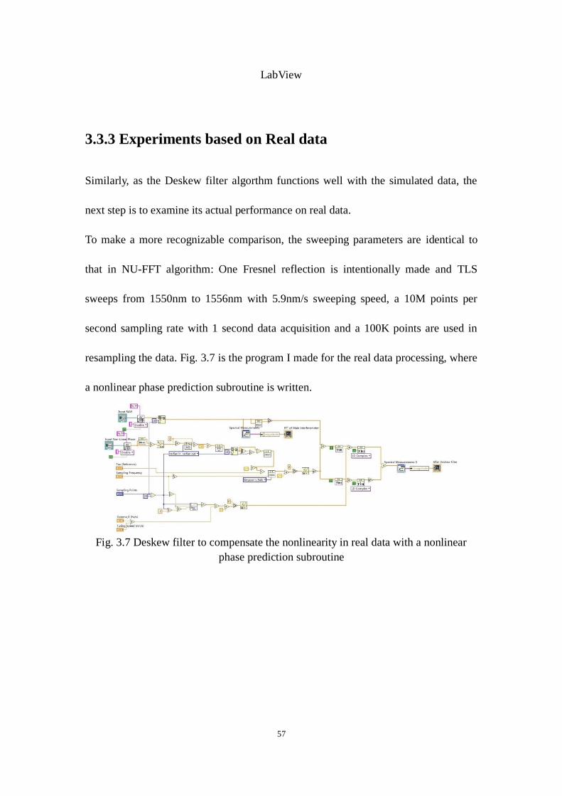
57
LabView
3.3.3 Experiments based on Real data
Similarly, as the Deskew filter algorthm functions well with the simulated data, the
next step is to examine its actual performance on real data.
To make a more recognizable comparison, the sweeping parameters are identical to
that in NU-FFT algorithm: One Fresnel reflection is intentionally made and TLS
sweeps from 1550nm to 1556nm with 5.9nm/s sweeping speed, a 10M points per
second sampling rate with 1 second data acquisition and a 100K points are used in
resampling the data. Fig. 3.7 is the program I made for the real data processing, where
a nonlinear phase prediction subroutine is written.
Fig. 3.7 Deskew filter to compensate the nonlinearity in real data with a nonlinear
phase prediction subroutine
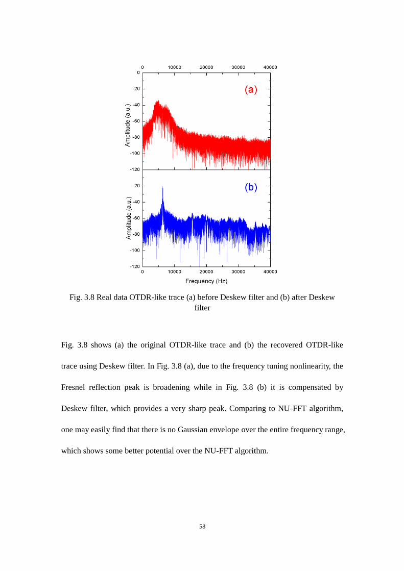
58
Fig. 3.8 Real data OTDR-like trace (a) before Deskew filter and (b) after Deskew
filter
Fig. 3.8 shows (a) the original OTDR-like trace and (b) the recovered OTDR-like
trace using Deskew filter. In Fig. 3.8 (a), due to the frequency tuning nonlinearity, the
Fresnel reflection peak is broadening while in Fig. 3.8 (b) it is compensated by
Deskew filter, which provides a very sharp peak. Comparing to NU-FFT algorithm,
one may easily find that there is no Gaussian envelope over the entire frequency range,
which shows some better potential over the NU-FFT algorithm.
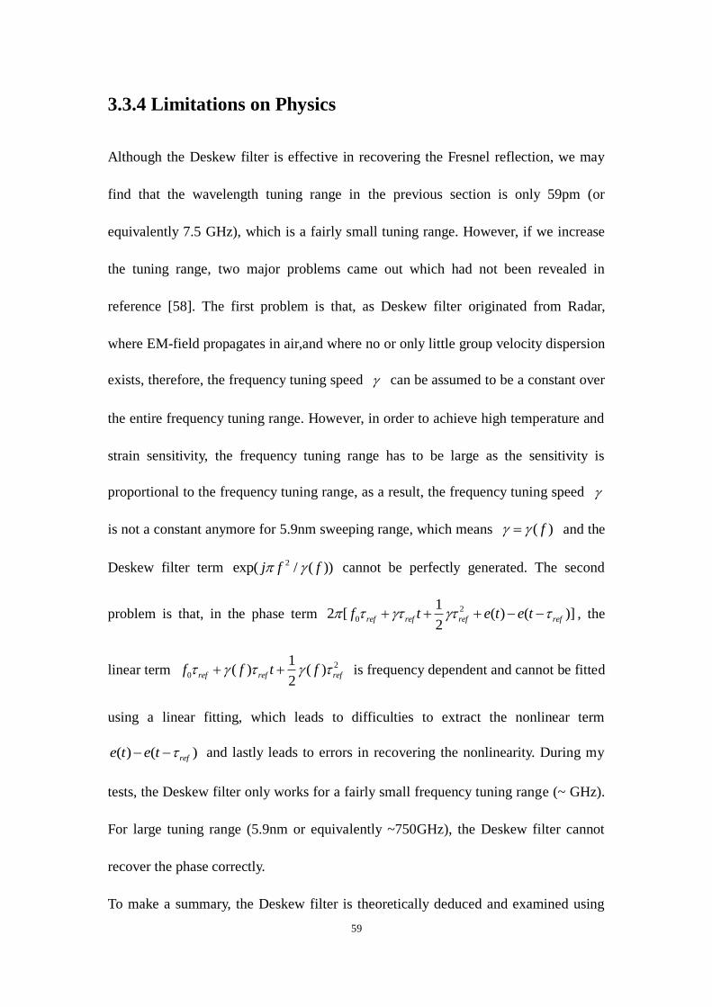
59
3.3.4 Limitations on Physics
Although the Deskew filter is effective in recovering the Fresnel reflection, we may
find that the wavelength tuning range in the previous section is only 59pm (or
equivalently 7.5 GHz), which is a fairly small tuning range. However, if we increase
the tuning range, two major problems came out which had not been revealed in
reference [58]. The first problem is that, as Deskew filter originated from Radar,
where EM-field propagates in air,and where no or only little group velocity dispersion
exists, therefore, the frequency tuning speed can be assumed to be a constant over
the entire frequency tuning range. However, in order to achieve high temperature and
strain sensitivity, the frequency tuning range has to be large as the sensitivity is
proportional to the frequency tuning range, as a result, the frequency tuning speed
is not a constant anymore for 5.9nm sweeping range, which means ( )f and the
Deskew filter term 2exp( / ( ))j f f cannot be perfectly generated. The second
problem is that, in the phase term 2
0
12 [ ( ) ( )]
2ref ref ref reff t e t e t , the
linear term 2
0
1( ) ( )
2ref ref reff f t f is frequency dependent and cannot be fitted
using a linear fitting, which leads to difficulties to extract the nonlinear term
( ) ( )refe t e t and lastly leads to errors in recovering the nonlinearity. During my
tests, the Deskew filter only works for a fairly small frequency tuning range (~ GHz).
For large tuning range (5.9nm or equivalently ~750GHz), the Deskew filter cannot
recover the phase correctly.
To make a summary, the Deskew filter is theoretically deduced and examined using
60
both simulated data and real data. For a simulated Fresnel reflection point, the
Deskew filter compensates the nonlinearity effectively as nonlinear phase was
predicted perfectly, a more than 10 times spatial resolution was found. However,
when it comes to real data, as the frequency tuning speed ( )f is a function of
optical frequency, the larger the frequency tuning range, the more ( )f changes and
leads to poorer compensation. Therefore, the Deskew filter only works for a small
frequency tuning range and cannot be adapted in temperature or strain sensing which
requires a large frequency tuning range.
3.4 Cubic Spline Interpolation
The third approach we proposed to treat tuning nonlinearities of OFDR is also a
resampling scheme. There are limits of previous approaches: NU-FFT is found to be
only working at short distance within the whole sensing range, and Deskew filter is
only capable for a small wavelength tuning range. Considering all those drawbacks,
the cubic spline interpolation approach is demonstrated to be able to function within a
large wavelength tuning range as well as to maintain high resampling accuracy.
3.4.1 Theory of Cubic spline interpolation
The cubic spline interpolation is a form of interpolation where the interpolant is a
special type of piecewise polynomial named a spline. Spline interpolation is favorable
61
over other polynomial interpolation because the interpolation error can be made trivial
even when low degree polynomials are employed for the spline. Another advantage is
that spline interpolation avoids the problem of Runge's phenomenon, which occurs
when employing higher order polynomial interpolation [68].
Now suppose a polynomial q(x) has the following values [69, 70]:
1 1
2 2
1 1
2 2
( )
( )
'( )
'( )
q x y
q x y
q x k
q x k
(3.19)
A symmetrical form can be written using above parameters:
1 2(1 ) (1 )( (1 ) )q t y ty t t a t bt (3.20)
where 1
2 1
x xt
x x and,
1 2 1 2 1
2 2 1 2 1
( ) ( )
( ) ( )
a k x x y y
b k x x y y
(3.21)
As 2 1
1' /
dq dt dqq dq dx
dt dx dt x x, one may get first order derivative,
2 1
2 1 2 1 2 1
(1 )' (1 2 ) (1 )
y y a t bt b aq t t t
x x x x x x
(3.22)
And second order derivative,
2
2 1
2 ( )3'' 2
( )
b a a b tq
x x
(3.23)
Setting 1x x and 2x x respectively in Eq. (3.22), one may verify the first order
derivatives 1 1q '(x ) k and 2 2q '(x ) k are automatically satisfied. The second
order derivatives are as follows:
62
1 2
2 1
2 2
2 1
2''( ) 2
( )
2''( ) 2
( )
b aq x
x x
a bq x
x x
(3.24)
Above discussion is based on two points interpolation, if a data set with n points is to
be interpolated, the interpolated curve has the form of:
1(1 ) (1 )( (1 ) )i i i i iq t y ty t t a t bt (3.25)
where 1,2,...,i n and 1
1
i
i i
x xt
x x are n polynomials interpolating y in the interval
1 i ix x x for 1,2,...,i n such that the first order derivative 1' ( ) ' ( )i i i iq x q x at
each point. Those n polynomials define a differentiable curve within 0 nx x x .
Similarly, we have definition for a and b:
1 1 1
1 1
( ) ( )
( ) ( )
i i i i i i
i i i i i i
a k x x y y
b k x x y y
(3.26)
And
0 1 0
1
' ( )
' ( ) ' ( ), 1,2,..., 1
' ( )
i i i i i
n n n
k q x
k q x q x i n
k q x
(3.27)
The above equations give a smooth curve with continuous first order derivative at
each knot. A more smooth curve with continuous second order derivative can be
obtained if the sequence 1 2, ,..., nk k k satisfies 1'' ( ) '' ( )i i i iq x q x .
From Eq. (3.24), (3.25), (3.26), (3.27) we may find this is the case if and only if
1 1 1 1
2 2
1 1 1 1 1 1
1 12 3
( ) ( )
i i i i i ii
i i i i i i i i i i i i
k k y y y yk
x x x x x x x x x x x x
(3.28)
For 1,2,...,i n , the relations above are n-1 linear equations for n+1 values
63
1 2 1, ,..., nk k k .
At the boundary where 0x x and nx x , the second order derivatives are
intentionally made zero, in which way 0k and nk are determined:
1 0 1 0 1 01 0 2
1 0
1 1 1
2
1
3( ) ( 2 )( )'' ( ) 2 0,
( )
3( ) (2 )( )'' ( ) 2 0,
( )
n n n n n nn n
n n
y y k k x xq x
x x
y y k k x xq x
x x
(3.29)
Finally, Eq. (3.28) together with Eq. (3.29) constitute n+1 linear equations that
interpolate n curves with continuous first order derivative and second order derivative.
This interpolation scheme is named cubic spline interpolation as it is a third order
polynomial fitting.
3.4.2 Applying cubic spline interpolation in data resampling
Similar to NU-FFT and deskew filter, cubic spline interpolation requires non-equal
spaced instantaneous optical frequency, which can be subtracted from auxiliary
interferometer. The beat signal generated from the auxiliary interferometer can be
expressed as [57],
0( ) cos 2 ( )I t U v t (3.30)
where U0 is the amplitude of the beat signal, τ is the group delay difference between
the two arms of the MZI, and v(t) is the instantaneous optical frequency of the TLS
which can be recovered by use of the Hilbert transform,
1
H( ) tan ( ) ( ) 2v t I t I t (3.31)
Where
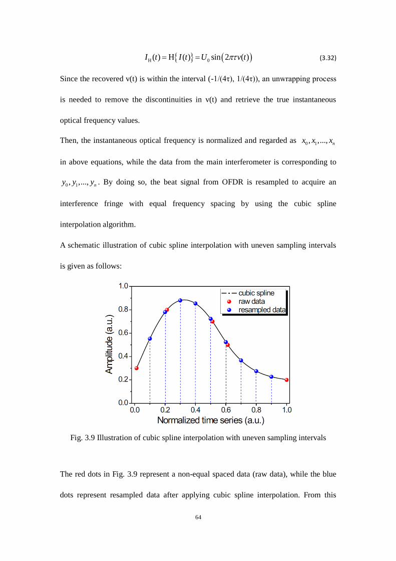
64
H 0( ) H ( ) sin 2 ( )I t I t U v t (3.32)
Since the recovered v(t) is within the interval (-1/(4τ), 1/(4τ)), an unwrapping process
is needed to remove the discontinuities in v(t) and retrieve the true instantaneous
optical frequency values.
Then, the instantaneous optical frequency is normalized and regarded as 0 1, ,..., nx x x
in above equations, while the data from the main interferometer is corresponding to
0 1, ,..., ny y y . By doing so, the beat signal from OFDR is resampled to acquire an
interference fringe with equal frequency spacing by using the cubic spline
interpolation algorithm.
A schematic illustration of cubic spline interpolation with uneven sampling intervals
is given as follows:
Fig. 3.9 Illustration of cubic spline interpolation with uneven sampling intervals
The red dots in Fig. 3.9 represent a non-equal spaced data (raw data), while the blue
dots represent resampled data after applying cubic spline interpolation. From this
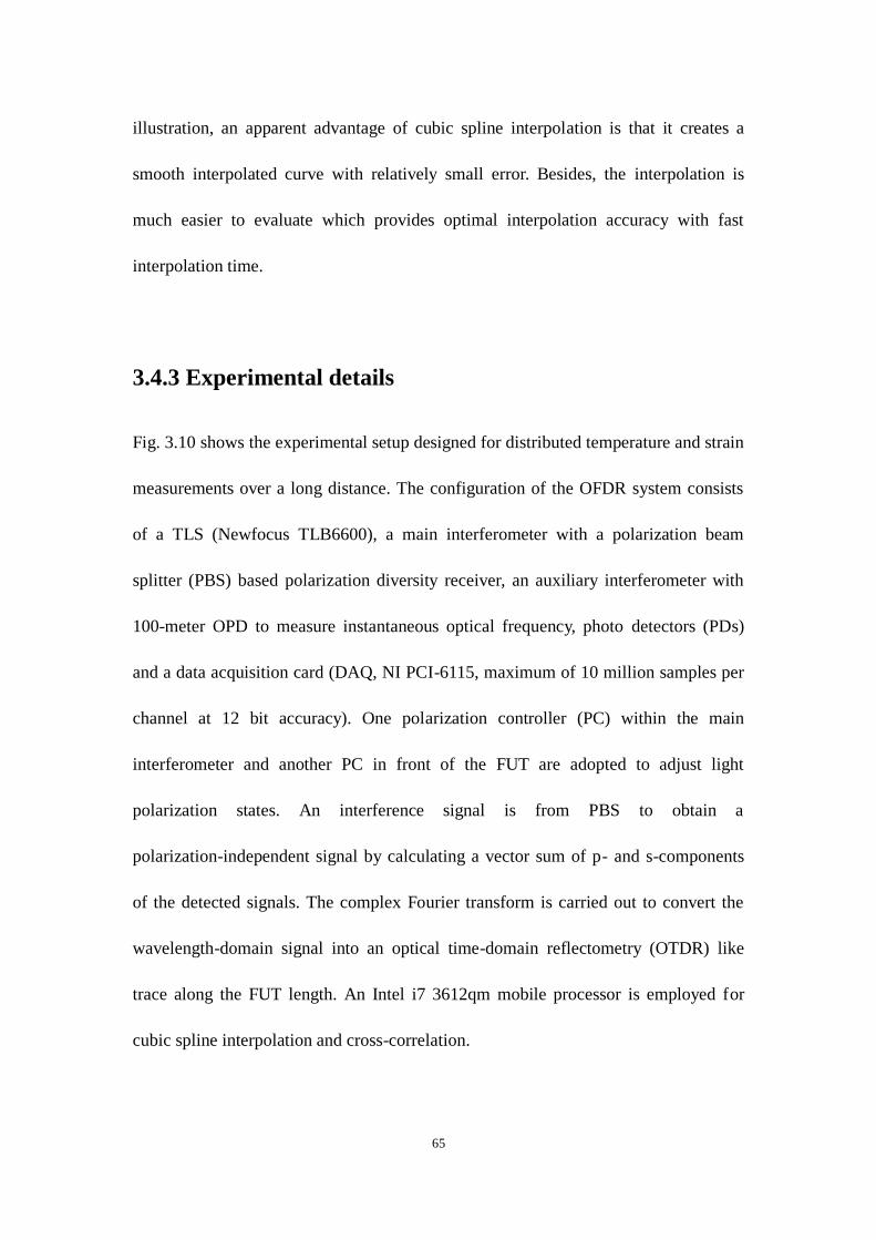
65
illustration, an apparent advantage of cubic spline interpolation is that it creates a
smooth interpolated curve with relatively small error. Besides, the interpolation is
much easier to evaluate which provides optimal interpolation accuracy with fast
interpolation time.
3.4.3 Experimental details
Fig. 3.10 shows the experimental setup designed for distributed temperature and strain
measurements over a long distance. The configuration of the OFDR system consists
of a TLS (Newfocus TLB6600), a main interferometer with a polarization beam
splitter (PBS) based polarization diversity receiver, an auxiliary interferometer with
100-meter OPD to measure instantaneous optical frequency, photo detectors (PDs)
and a data acquisition card (DAQ, NI PCI-6115, maximum of 10 million samples per
channel at 12 bit accuracy). One polarization controller (PC) within the main
interferometer and another PC in front of the FUT are adopted to adjust light
polarization states. An interference signal is from PBS to obtain a
polarization-independent signal by calculating a vector sum of p- and s-components
of the detected signals. The complex Fourier transform is carried out to convert the
wavelength-domain signal into an optical time-domain reflectometry (OTDR) like
trace along the FUT length. An Intel i7 3612qm mobile processor is employed for
cubic spline interpolation and cross-correlation.
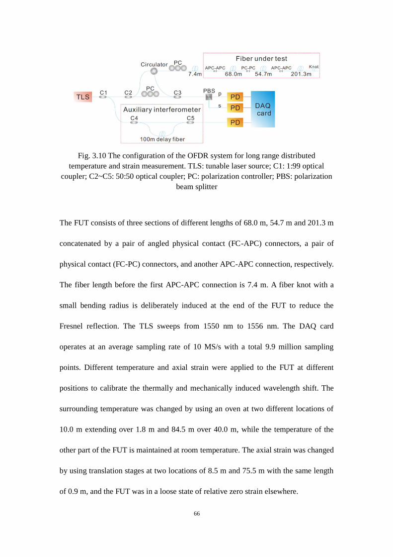
66
Fig. 3.10 The configuration of the OFDR system for long range distributed
temperature and strain measurement. TLS: tunable laser source; C1: 1:99 optical
coupler; C2~C5: 50:50 optical coupler; PC: polarization controller; PBS: polarization
beam splitter
The FUT consists of three sections of different lengths of 68.0 m, 54.7 m and 201.3 m
concatenated by a pair of angled physical contact (FC-APC) connectors, a pair of
physical contact (FC-PC) connectors, and another APC-APC connection, respectively.
The fiber length before the first APC-APC connection is 7.4 m. A fiber knot with a
small bending radius is deliberately induced at the end of the FUT to reduce the
Fresnel reflection. The TLS sweeps from 1550 nm to 1556 nm. The DAQ card
operates at an average sampling rate of 10 MS/s with a total 9.9 million sampling
points. Different temperature and axial strain were applied to the FUT at different
positions to calibrate the thermally and mechanically induced wavelength shift. The
surrounding temperature was changed by using an oven at two different locations of
10.0 m extending over 1.8 m and 84.5 m over 40.0 m, while the temperature of the
other part of the FUT is maintained at room temperature. The axial strain was changed
by using translation stages at two locations of 8.5 m and 75.5 m with the same length
of 0.9 m, and the FUT was in a loose state of relative zero strain elsewhere.
67
3.4.4 Experimental results and discussion
3.4.4.1 OTDR-like trace
For long-range distributed sensing, good location accuracy is highly desired in
addition to the high temperature and strain resolution detection of changes in
environmental variables. Thus an OTDR-like trace is firstly acquired to locate
temperature changing and strain applied positions on the optical fiber. The spatial
resolution ΔZ is determined by the sweep frequency range ΔF, following the formula
of ΔZ = c/(2nΔF), where c is the speed of light in vacuum and n is the group index of
the fiber [50]. The theoretical spatial resolution for 5.9 nm swept range is calculated
to be 0.14 mm.
Fig. 3.11 OTDR-like traces (a) before and (b) after using cubic spline interpolation.
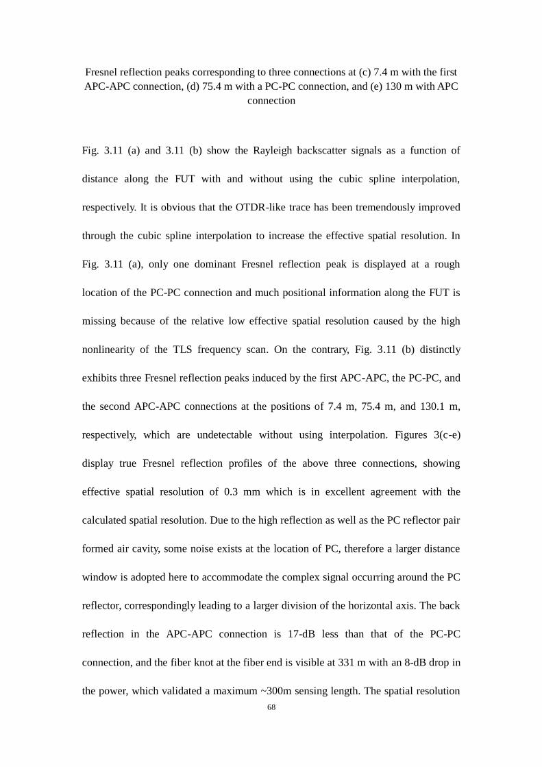
68
Fresnel reflection peaks corresponding to three connections at (c) 7.4 m with the first
APC-APC connection, (d) 75.4 m with a PC-PC connection, and (e) 130 m with APC
connection
Fig. 3.11 (a) and 3.11 (b) show the Rayleigh backscatter signals as a function of
distance along the FUT with and without using the cubic spline interpolation,
respectively. It is obvious that the OTDR-like trace has been tremendously improved
through the cubic spline interpolation to increase the effective spatial resolution. In
Fig. 3.11 (a), only one dominant Fresnel reflection peak is displayed at a rough
location of the PC-PC connection and much positional information along the FUT is
missing because of the relative low effective spatial resolution caused by the high
nonlinearity of the TLS frequency scan. On the contrary, Fig. 3.11 (b) distinctly
exhibits three Fresnel reflection peaks induced by the first APC-APC, the PC-PC, and
the second APC-APC connections at the positions of 7.4 m, 75.4 m, and 130.1 m,
respectively, which are undetectable without using interpolation. Figures 3(c-e)
display true Fresnel reflection profiles of the above three connections, showing
effective spatial resolution of 0.3 mm which is in excellent agreement with the
calculated spatial resolution. Due to the high reflection as well as the PC reflector pair
formed air cavity, some noise exists at the location of PC, therefore a larger distance
window is adopted here to accommodate the complex signal occurring around the PC
reflector, correspondingly leading to a larger division of the horizontal axis. The back
reflection in the APC-APC connection is 17-dB less than that of the PC-PC
connection, and the fiber knot at the fiber end is visible at 331 m with an 8-dB drop in
the power, which validated a maximum ~300m sensing length. The spatial resolution
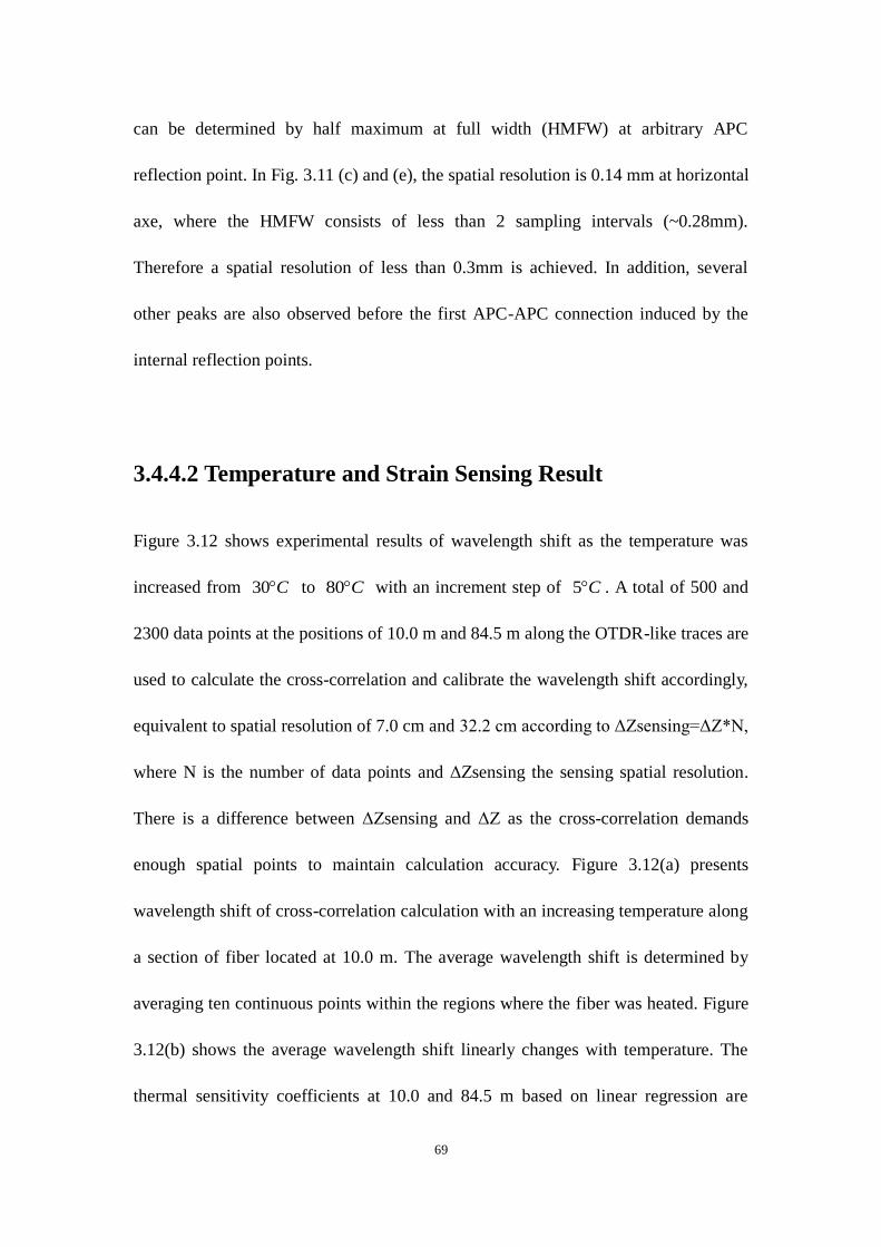
69
can be determined by half maximum at full width (HMFW) at arbitrary APC
reflection point. In Fig. 3.11 (c) and (e), the spatial resolution is 0.14 mm at horizontal
axe, where the HMFW consists of less than 2 sampling intervals (~0.28mm).
Therefore a spatial resolution of less than 0.3mm is achieved. In addition, several
other peaks are also observed before the first APC-APC connection induced by the
internal reflection points.
3.4.4.2 Temperature and Strain Sensing Result
Figure 3.12 shows experimental results of wavelength shift as the temperature was
increased from 30 C to 80 C with an increment step of 5 C . A total of 500 and
2300 data points at the positions of 10.0 m and 84.5 m along the OTDR-like traces are
used to calculate the cross-correlation and calibrate the wavelength shift accordingly,
equivalent to spatial resolution of 7.0 cm and 32.2 cm according to ΔZsensing=ΔZ*N,
where N is the number of data points and ΔZsensing the sensing spatial resolution.
There is a difference between ΔZsensing and ΔZ as the cross-correlation demands
enough spatial points to maintain calculation accuracy. Figure 3.12(a) presents
wavelength shift of cross-correlation calculation with an increasing temperature along
a section of fiber located at 10.0 m. The average wavelength shift is determined by
averaging ten continuous points within the regions where the fiber was heated. Figure
3.12(b) shows the average wavelength shift linearly changes with temperature. The
thermal sensitivity coefficients at 10.0 and 84.5 m based on linear regression are
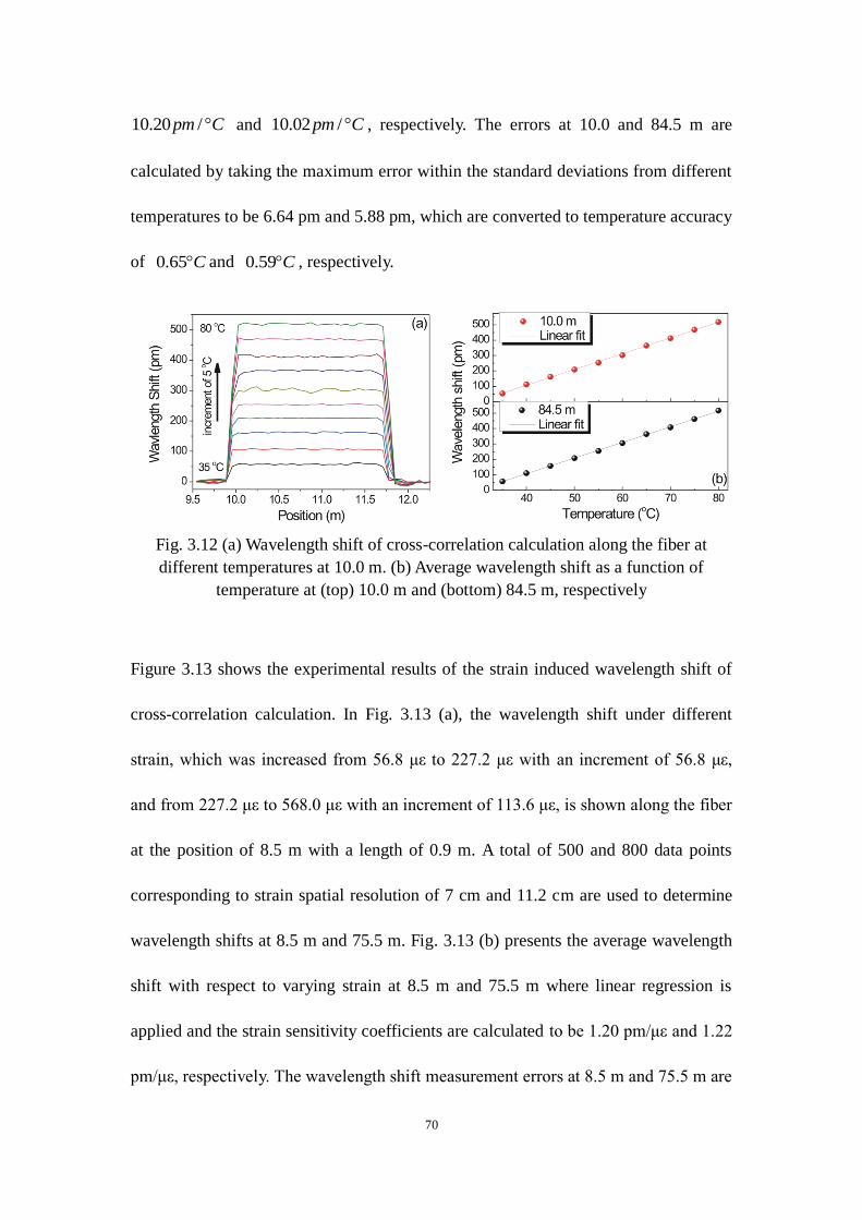
70
10.20 /pm C and 10.02 /pm C , respectively. The errors at 10.0 and 84.5 m are
calculated by taking the maximum error within the standard deviations from different
temperatures to be 6.64 pm and 5.88 pm, which are converted to temperature accuracy
of 0.65 C and 0.59 C , respectively.
Fig. 3.12 (a) Wavelength shift of cross-correlation calculation along the fiber at
different temperatures at 10.0 m. (b) Average wavelength shift as a function of
temperature at (top) 10.0 m and (bottom) 84.5 m, respectively
Figure 3.13 shows the experimental results of the strain induced wavelength shift of
cross-correlation calculation. In Fig. 3.13 (a), the wavelength shift under different
strain, which was increased from 56.8 με to 227.2 με with an increment of 56.8 με,
and from 227.2 με to 568.0 με with an increment of 113.6 με, is shown along the fiber
at the position of 8.5 m with a length of 0.9 m. A total of 500 and 800 data points
corresponding to strain spatial resolution of 7 cm and 11.2 cm are used to determine
wavelength shifts at 8.5 m and 75.5 m. Fig. 3.13 (b) presents the average wavelength
shift with respect to varying strain at 8.5 m and 75.5 m where linear regression is
applied and the strain sensitivity coefficients are calculated to be 1.20 pm/με and 1.22
pm/με, respectively. The wavelength shift measurement errors at 8.5 m and 75.5 m are
71
1.82 pm and 2.80 pm, corresponding to strain accuracy of 1.5 με and 2.3 με,
respectively.
Fig. 3.13 (a) Wavelength shift of cross-correlation calculation along the fiber under
different strain at 8.5 m. (b) Average wavelength shift as a function of strain at (top)
8.5 m and (bottom) 75.5 m, respectively
3.4.4.3 Spatial Resolution at different distances
In temperature and strain sensing experiments, it is found that the sensing resolution
deteriorates as the fiber length extends. In order to determine the actual sensing
resolution, the number of data points needed for obtaining an optimum
cross-correlation figure with a minimum side peak suppression ratio of 2 is calculated.
The cross-correlation figures at three different locations of 10 m, 140 m, and 310 m
using 500, 2800, and 6000 data points in the temperature measurement are illustrated
in Fig. 3.14, which indicates that the predicted temperature spatial resolution are
about 7 cm, 39 cm and 84 cm, respectively, as shown in Figs. 3.14(a-c). In addition,
the temperature spatial resolution at different locations (10, 50 and 150 m) along the
FUT as a function of the wavelength tuning speed is shown in Fig. 3.15. It is found
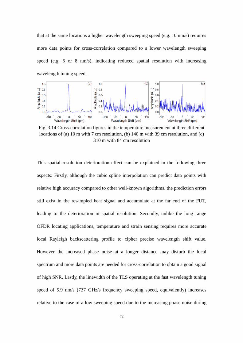
72
that at the same locations a higher wavelength sweeping speed (e.g. 10 nm/s) requires
more data points for cross-correlation compared to a lower wavelength sweeping
speed (e.g. 6 or 8 nm/s), indicating reduced spatial resolution with increasing
wavelength tuning speed.
Fig. 3.14 Cross-correlation figures in the temperature measurement at three different
locations of (a) 10 m with 7 cm resolution, (b) 140 m with 39 cm resolution, and (c)
310 m with 84 cm resolution
This spatial resolution deterioration effect can be explained in the following three
aspects: Firstly, although the cubic spline interpolation can predict data points with
relative high accuracy compared to other well-known algorithms, the prediction errors
still exist in the resampled beat signal and accumulate at the far end of the FUT,
leading to the deterioration in spatial resolution. Secondly, unlike the long range
OFDR locating applications, temperature and strain sensing requires more accurate
local Rayleigh backscattering profile to cipher precise wavelength shift value.
However the increased phase noise at a longer distance may disturb the local
spectrum and more data points are needed for cross-correlation to obtain a good signal
of high SNR. Lastly, the linewidth of the TLS operating at the fast wavelength tuning
speed of 5.9 nm/s (737 GHz/s frequency sweeping speed, equivalently) increases
relative to the case of a low sweeping speed due to the increasing phase noise during
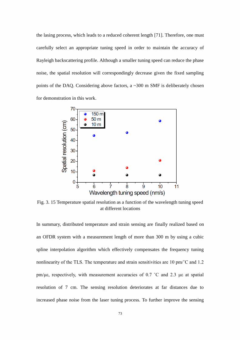
73
the lasing process, which leads to a reduced coherent length [71]. Therefore, one must
carefully select an appropriate tuning speed in order to maintain the accuracy of
Rayleigh backscattering profile. Although a smaller tuning speed can reduce the phase
noise, the spatial resolution will correspondingly decrease given the fixed sampling
points of the DAQ. Considering above factors, a ~300 m SMF is deliberately chosen
for demonstration in this work.
Fig. 3. 15 Temperature spatial resolution as a function of the wavelength tuning speed
at different locations
In summary, distributed temperature and strain sensing are finally realized based on
an OFDR system with a measurement length of more than 300 m by using a cubic
spline interpolation algorithm which effectively compensates the frequency tuning
nonlinearity of the TLS. The temperature and strain sensitivities are 10 pm/˚C and 1.2
pm/με, respectively, with measurement accuracies of 0.7 ˚C and 2.3 με at spatial
resolution of 7 cm. The sensing resolution deteriorates at far distances due to
increased phase noise from the laser tuning process. To further improve the sensing

74
distance and spatial resolution, one may use a TLS with a large tuning range and a
slower tuning speed, and a DAQ card of a large on-board memory buffer combined
with a powerful computer. The proposed technique enables an extended sensing
distance with excellent spatial resolution, spectral sensitivity, and measurement
accuracy over other traditional nonlinearly-triggered OFDR systems, and has great
potential in a variety of practical sensing applications such as structural health
monitoring of civil infrastructure systems.
75
Chapter 4
Enhanced Temperature Response Sensing
based on OFDR
4.1 Review and Principle of temperature sensing
In this section we shall review the principles of temperature sensing using OFDR. As
discussed in Chapter 2.2.3, OFDR detects the temperature, strain or any other
environmental perturbations by measuring the local wavelength shift, where a number
of spatial points are used for cross-correlation. A formula describing this relationship
between wavelength shift and temperature change is given as follows [4]:
/ TK T (4.1)
where TK is a thermal coefficient that describes the response of the fiber and
consists of two terms [4]. The first term – thermal expansion coefficient involves
all materials that contribute to the fiber. Specifically, bare fiber made out of pure silica
has a typical value of 6 10.55 10 K
[50]. When fiber is coated by acrylate
( 6 1140 0 K
), the thermal expansion coefficient is a weighted value of coating
and bare fiber, which corresponds to a larger . The second term – thermal optic
coefficient n is defined by /dn dT which describes the refractive index change
with respect to temperature. n is a constant for a given material and is regardless of
waveguide shape with a typical value of 6 16.1 10n K [50].Taking both and
76
n into account, the thermal coefficient for SMF is 6 1~ 7.0 10T nK K
.
Thus a linear wavelength shift is expected at a moderate temperature range, while
typical temperature response at 1550nm is 1/ 10.85TT K pm K .
The above analysis provides a potential approach to enhance the temperature response:
either enhance thermal expansion coefficient or enhance thermal optic coefficient. In
the next two sections, two approaches aiming at enhancing the temperature response
are individually discussed.
4.2 Enhanced temperature sensitivity based on OFDR with
SMF
4.2.1 Principle of enhancing temperature response
As stated in 4.1, the temperature response to two terms: thermal expansion coefficient
and thermal optic coefficient n . Since n is a constant for given material, the
only possible approach to enhance temperature response is to enlarge which is a
weighed value of coating and bare fiber. Following this idea, a coating with large
thermal expansion coefficient and thickness would potentially enhance .
4.2.2 Experiment Set-up
Fig. 4.1 shows the experimental set-up to measure distributed Rayleigh backscattering
light. The configuration of the OFDR system consists of a TLS (Newfocus TLB6600),
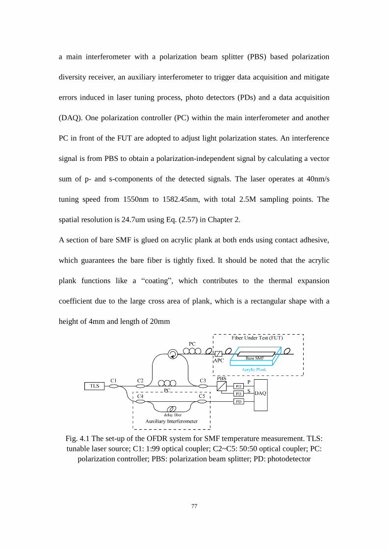
77
a main interferometer with a polarization beam splitter (PBS) based polarization
diversity receiver, an auxiliary interferometer to trigger data acquisition and mitigate
errors induced in laser tuning process, photo detectors (PDs) and a data acquisition
(DAQ). One polarization controller (PC) within the main interferometer and another
PC in front of the FUT are adopted to adjust light polarization states. An interference
signal is from PBS to obtain a polarization-independent signal by calculating a vector
sum of p- and s-components of the detected signals. The laser operates at 40nm/s
tuning speed from 1550nm to 1582.45nm, with total 2.5M sampling points. The
spatial resolution is 24.7um using Eq. (2.57) in Chapter 2.
A section of bare SMF is glued on acrylic plank at both ends using contact adhesive,
which guarantees the bare fiber is tightly fixed. It should be noted that the acrylic
plank functions like a “coating”, which contributes to the thermal expansion
coefficient due to the large cross area of plank, which is a rectangular shape with a
height of 4mm and length of 20mm
Fig. 4.1 The set-up of the OFDR system for SMF temperature measurement. TLS:
tunable laser source; C1: 1:99 optical coupler; C2~C5: 50:50 optical coupler; PC:
polarization controller; PBS: polarization beam splitter; PD: photodetector
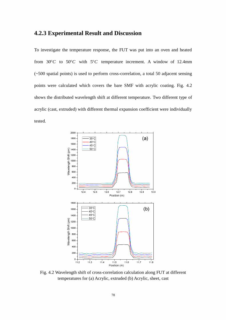
78
4.2.3 Experimental Result and Discussion
To investigate the temperature response, the FUT was put into an oven and heated
from 30 C to 50 C with 5 C temperature increment. A window of 12.4mm
(~500 spatial points) is used to perform cross-correlation, a total 50 adjacent sensing
points were calculated which covers the bare SMF with acrylic coating. Fig. 4.2
shows the distributed wavelength shift at different temperature. Two different type of
acrylic (cast, extruded) with different thermal expansion coefficient were individually
tested.
Fig. 4.2 Wavelength shift of cross-correlation calculation along FUT at different
temperatures for (a) Acrylic, extruded (b) Acrylic, sheet, cast
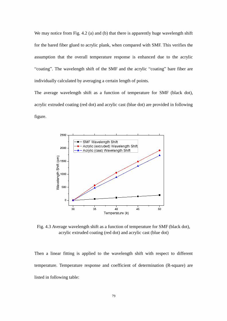
79
We may notice from Fig. 4.2 (a) and (b) that there is apparently huge wavelength shift
for the bared fiber glued to acrylic plank, when compared with SMF. This verifies the
assumption that the overall temperature response is enhanced due to the acrylic
“coating”. The wavelength shift of the SMF and the acrylic “coating” bare fiber are
individually calculated by averaging a certain length of points.
The average wavelength shift as a function of temperature for SMF (black dot),
acrylic extruded coating (red dot) and acrylic cast (blue dot) are provided in following
figure.
Fig. 4.3 Average wavelength shift as a function of temperature for SMF (black dot),
acrylic extruded coating (red dot) and acrylic cast (blue dot)
Then a linear fitting is applied to the wavelength shift with respect to different
temperature. Temperature response and coefficient of determination (R-square) are
listed in following table:
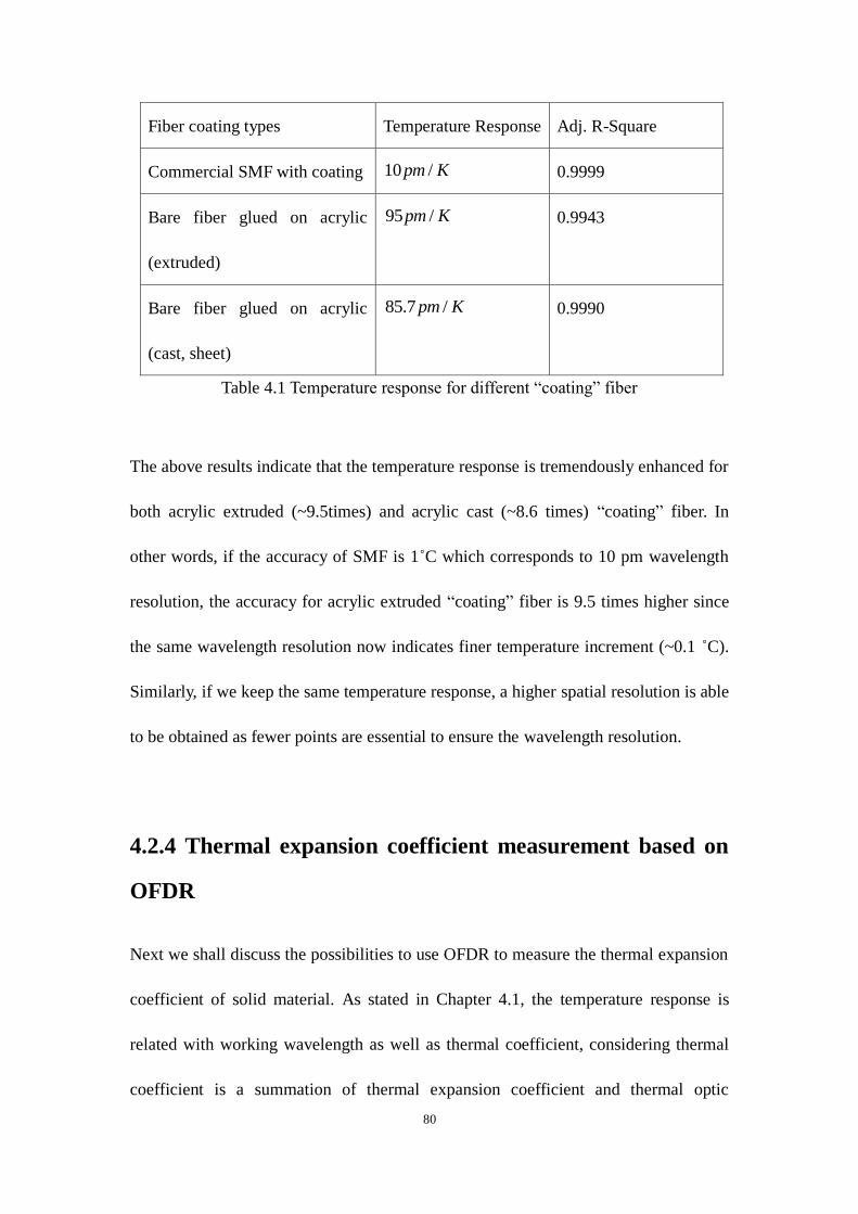
80
Fiber coating types Temperature Response Adj. R-Square
Commercial SMF with coating 10 /pm K 0.9999
Bare fiber glued on acrylic
(extruded)
95 /pm K 0.9943
Bare fiber glued on acrylic
(cast, sheet)
85.7 /pm K 0.9990
Table 4.1 Temperature response for different “coating” fiber
The above results indicate that the temperature response is tremendously enhanced for
both acrylic extruded (~9.5times) and acrylic cast (~8.6 times) “coating” fiber. In
other words, if the accuracy of SMF is 1˚C which corresponds to 10 pm wavelength
resolution, the accuracy for acrylic extruded “coating” fiber is 9.5 times higher since
the same wavelength resolution now indicates finer temperature increment (~0.1 ˚C).
Similarly, if we keep the same temperature response, a higher spatial resolution is able
to be obtained as fewer points are essential to ensure the wavelength resolution.
4.2.4 Thermal expansion coefficient measurement based on
OFDR
Next we shall discuss the possibilities to use OFDR to measure the thermal expansion
coefficient of solid material. As stated in Chapter 4.1, the temperature response is
related with working wavelength as well as thermal coefficient, considering thermal
coefficient is a summation of thermal expansion coefficient and thermal optic
81
coefficient, we have the following equation:
( )T T nR K (4.2)
In this way, the thermal expansion coefficient can be calculated by:
/T nR (4.3)
If we glue any solid material to fiber that function like a “coating”, the solid material
will contribute to thermal expansion coefficient since is a weighted value of both
coating and fiber. However, if the cross area of coating is much larger than that of
fiber, is approximately _ coating
. Therefore, the thermal expansion coefficient
could be determined.
Following this idea, we calculated for both acrylic extruded and acrylic cast,
with values of 6 155.2 10 /m mK and
6 149.2 10 /m mK , respectively. In
comparison, typical acrylic has a value of 6 172 10 /m mK , which is slightly larger
than the value of our approach. This is reasonable since the acrylic plank employed in
this experiment is not thick enough to ignore fiber, resulting in a lower weighted value.
Further works shall be done to increase the accuracy.
We proposed an approach to enhance the temperature response of OFDR by adding a
“coating” with large thermal expansion coefficient. This large thermal expansion
coefficient will contribute to overall thermal coefficient and therefore enhance the
temperature response. Specifically, ~9.5 times and ~8.6 times higher temperature
responses are achieved, using acrylic extruded and acrylic cast material as “coatings”.
To my knowledge, this is the first time an OFDR system is shown to perform high
temperature accuracy sensing. Inversely, it is also possible to measure thermal
82
expansion coefficient of solid materials. Further experiments shall be done for more
accurate results.
4.3 Taper based distributed temperature sensing using
OFDR
4.3.1 Introduction and Properties of Taper
Taper is a unique structure which has been studied for over 20 years and is named for
its reduced diameter at transition region with a taper like shape. Originally, taper is
used in fiber optical couplers where two fibers put in parallel are uniformly stretched
by flame or CO2 laser scanning [72, 73]. Since 2000, taper structures are widely
implemented in temperature, strain, displacement, humidity and vibration sensing [12,
74-78]. Tapering is a simple, efficient and low-cost technique to generate higher order
modes which can be employed in sensing by building interferometer structure.
Compared to other fiber sensors, taper has similar performance but are more easily
fabricated.
Taper can be also implemented in distributed sensing if a uniform taper waist
diameter is guaranteed. Recently, the thermal and mechanical properties of taper has
been studied using OFDR system [35], in which work a ~500 times higher strain
sensitivity is achieved using ~6μm diameter taper. Following this idea, a possible
approach to enhance the temperature sensitivity is to convert the temperature
measurement into strain measurement.
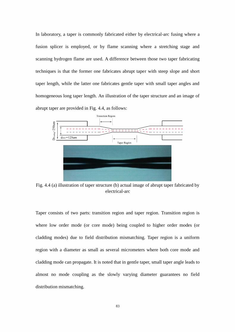
83
In laboratory, a taper is commonly fabricated either by electrical-arc fusing where a
fusion splicer is employed, or by flame scanning where a stretching stage and
scanning hydrogen flame are used. A difference between those two taper fabricating
techniques is that the former one fabricates abrupt taper with steep slope and short
taper length, while the latter one fabricates gentle taper with small taper angles and
homogeneous long taper length. An illustration of the taper structure and an image of
abrupt taper are provided in Fig. 4.4, as follows:
Fig. 4.4 (a) illustration of taper structure (b) actual image of abrupt taper fabricated by
electrical-arc
Taper consists of two parts: transition region and taper region. Transition region is
where low order mode (or core mode) being coupled to higher order modes (or
cladding modes) due to field distribution mismatching. Taper region is a uniform
region with a diameter as small as several micrometers where both core mode and
cladding mode can propagate. It is noted that in gentle taper, small taper angle leads to
almost no mode coupling as the slowly varying diameter guarantees no field
distribution mismatching.
84
4.3.2 Principle of Enhanced temperature response using
taper
In Chapter 4.2, we have proposed a SMF with acrylic “coating” has a temperature
response which is ~9.5 times than that of SMF, in which experiment the thermal
expansion coefficient is enhanced. Due to the fact that the diameter of taper is
extremely small in our experiment (1μm), the ratio between the cross area of acrylic
plank and the taper is much larger than that in Chap. 4.2. Therefore, the thermal
expansion coefficient of the taper on acrylic coating could be ultimately close to that
of acrylic coating, which is even larger than that in Chap. 4.2 and we could expect an
even larger temperature response as T nK .
4.3.3 Experiment Set-up
Fig. 4.5 shows the experiment set-up to measure distributed Rayleigh backscattering
light. The configuration of the OFDR system is quite similar with that in Chapter 4.2,
except that the FUT is a taper with 1µm diameter: It consists of a TLS, a main
interferometer with a polarization beam splitter (PBS) based polarization diversity
receiver, an auxiliary interferometer to trigger data acquisition, photo-detectors (PD)
and a data acquisition (DAQ). One polarization controller (PC) within the main
interferometer and another PC in front of the FUT are adopted to adjust light
polarization states. The PBS splits the interference signal into two orthogonal
polarization states to obtain a polarization-independent signal by calculating a vector
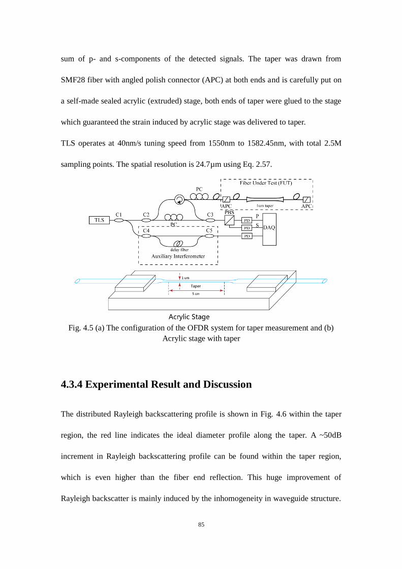
85
sum of p- and s-components of the detected signals. The taper was drawn from
SMF28 fiber with angled polish connector (APC) at both ends and is carefully put on
a self-made sealed acrylic (extruded) stage, both ends of taper were glued to the stage
which guaranteed the strain induced by acrylic stage was delivered to taper.
TLS operates at 40nm/s tuning speed from 1550nm to 1582.45nm, with total 2.5M
sampling points. The spatial resolution is 24.7µm using Eq. 2.57.
Fig. 4.5 (a) The configuration of the OFDR system for taper measurement and (b)
Acrylic stage with taper
4.3.4 Experimental Result and Discussion
The distributed Rayleigh backscattering profile is shown in Fig. 4.6 within the taper
region, the red line indicates the ideal diameter profile along the taper. A ~50dB
increment in Rayleigh backscattering profile can be found within the taper region,
which is even higher than the fiber end reflection. This huge improvement of
Rayleigh backscatter is mainly induced by the inhomogeneity in waveguide structure.
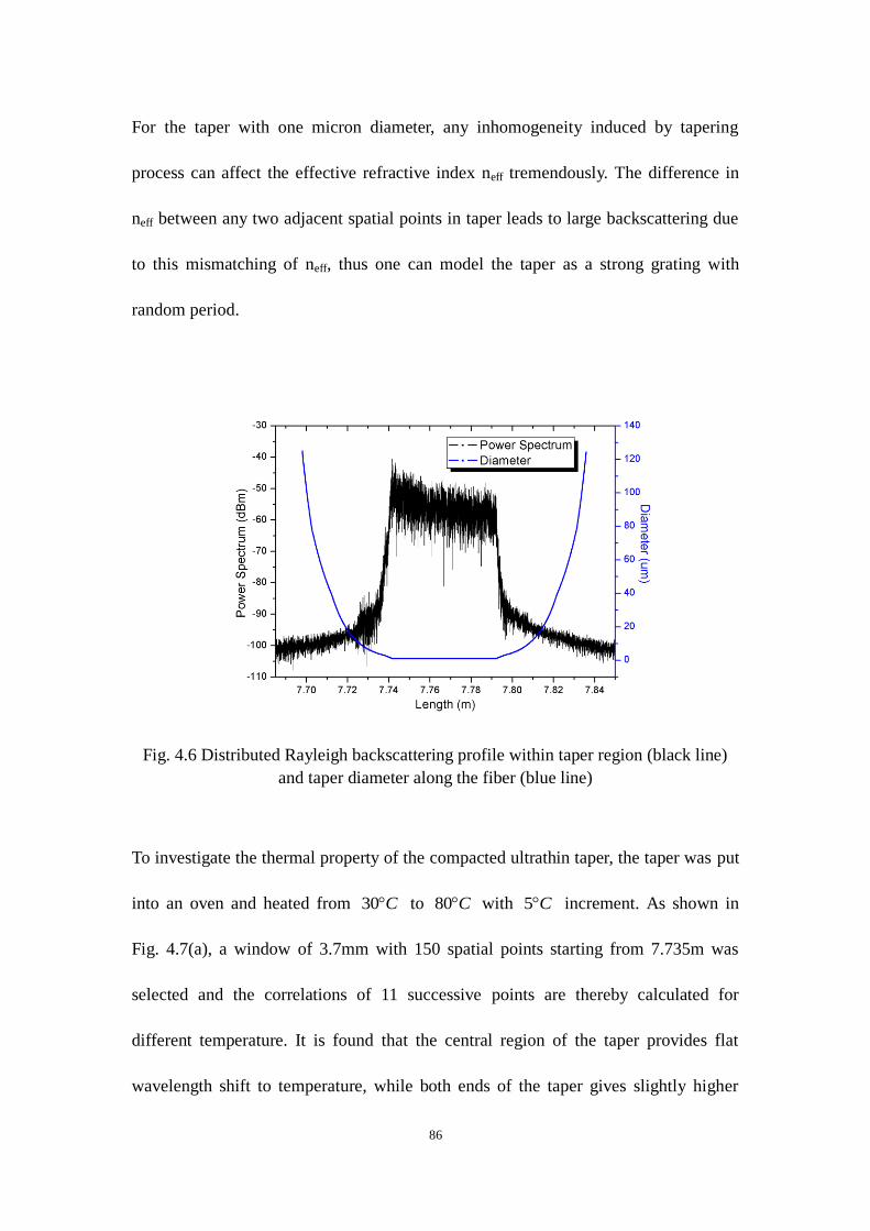
86
For the taper with one micron diameter, any inhomogeneity induced by tapering
process can affect the effective refractive index neff tremendously. The difference in
neff between any two adjacent spatial points in taper leads to large backscattering due
to this mismatching of neff, thus one can model the taper as a strong grating with
random period.
Fig. 4.6 Distributed Rayleigh backscattering profile within taper region (black line)
and taper diameter along the fiber (blue line)
To investigate the thermal property of the compacted ultrathin taper, the taper was put
into an oven and heated from 30 C to 80 C with 5 C increment. As shown in
Fig. 4.7(a), a window of 3.7mm with 150 spatial points starting from 7.735m was
selected and the correlations of 11 successive points are thereby calculated for
different temperature. It is found that the central region of the taper provides flat
wavelength shift to temperature, while both ends of the taper gives slightly higher
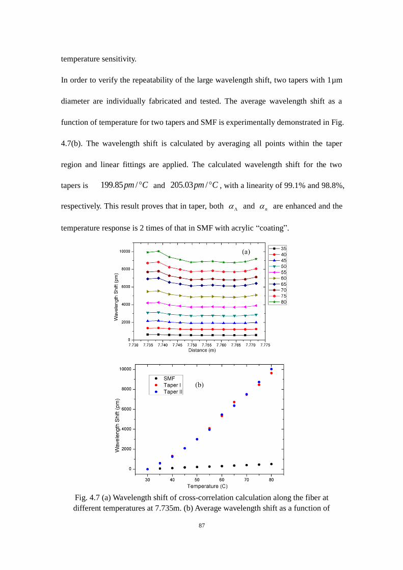
87
temperature sensitivity.
In order to verify the repeatability of the large wavelength shift, two tapers with 1µm
diameter are individually fabricated and tested. The average wavelength shift as a
function of temperature for two tapers and SMF is experimentally demonstrated in Fig.
4.7(b). The wavelength shift is calculated by averaging all points within the taper
region and linear fittings are applied. The calculated wavelength shift for the two
tapers is 199.85 /pm C and 205.03 /pm C , with a linearity of 99.1% and 98.8%,
respectively. This result proves that in taper, both and n are enhanced and the
temperature response is 2 times of that in SMF with acrylic “coating”.
Fig. 4.7 (a) Wavelength shift of cross-correlation calculation along the fiber at
different temperatures at 7.735m. (b) Average wavelength shift as a function of
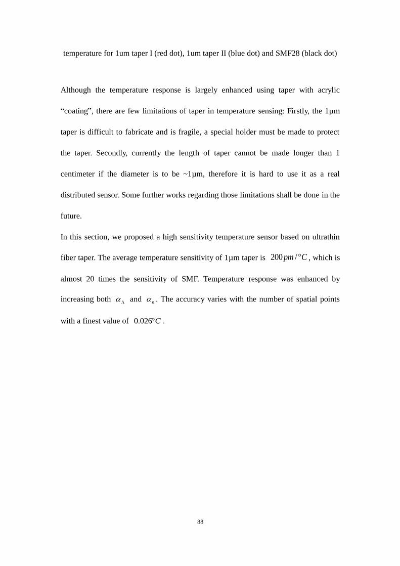
88
temperature for 1um taper I (red dot), 1um taper II (blue dot) and SMF28 (black dot)
Although the temperature response is largely enhanced using taper with acrylic
“coating”, there are few limitations of taper in temperature sensing: Firstly, the 1µm
taper is difficult to fabricate and is fragile, a special holder must be made to protect
the taper. Secondly, currently the length of taper cannot be made longer than 1
centimeter if the diameter is to be ~1µm, therefore it is hard to use it as a real
distributed sensor. Some further works regarding those limitations shall be done in the
future.
In this section, we proposed a high sensitivity temperature sensor based on ultrathin
fiber taper. The average temperature sensitivity of 1µm taper is 200 /pm C , which is
almost 20 times the sensitivity of SMF. Temperature response was enhanced by
increasing both and n . The accuracy varies with the number of spatial points
with a finest value of 0.026 C .
89
Chapter 5
Summary and Future Works
5.1 Summary
In this thesis, we presented two major works aimed at improving the performance and
applicability of OFDR: One aims at improving the sensing range while the other one
aims at enhancing the temperature response.
Firstly, we proposed three novel algorithms (NU-FFT, Deskew filter, Cubic spline
interpolation) to extend the working range of OFDR and an extended sensing range
OFDR with good temperature and strain accuracies is achieved. This is also the first
time an OFDR without triggered data acquisition is employed in distributed sensing.
Compared with traditional nonlinear triggered OFDR, the new configuration achieved
~4 times (~300m) sensing range than the commercial one (~70m). More specifically,
this new set-up is capable for sensing range as close as laser coherence length and
demands no further components. Thus it is a practical tool for long range distributed
sensing with high temperature and strain accuracy.
Secondly, the temperature response of sensing fiber is enhanced ~10 times (for acrylic
plank holder) and ~20 times (for ultrathin taper on acrylic plank holder), compared
with that of SMF. The principles behind this are to increase thermal coefficient which
consists of thermal expansion coefficient and thermal optic coefficient. In this work, a
90
bare fiber is fixed on acrylic plank, due to the large thermal expansion coefficient of
acrylic (~6 172 10 /m mK ), the weighted thermal expansion coefficient is
tremendously enhanced which in turn results in a large temperature response. For
ultrathin taper with 1µm diameter, thermal optic coefficient is enhanced due to the
waveguide geometry deformation. Therefore, the taper is experiencing an even higher
temperature response than bare fiber with acrylic “coating”. This work is especially
meaningful for its easy fabrication, low cost and extremely high temperature response
and leads to practical usage for high accuracy distributed temperature sensing.
5.2 Future Works
In this thesis, we improved the performance of OFDR in two aspects: Extending the
sensing range and enhancing the temperature response.
As the sensing range is primarily limited by TLS coherent length; one possible
approach to further stretch the sensing range is to increase the laser coherence length.
It is found that a TLS commonly has a longer coherence length if it works at a fairly
high tuning speed [79]. Following this idea, one could possibly achieve longer sensing
range and better spatial resolution by simply using high TLS tuning speed (~10nm/s
or higher). In this way, a high speed DAQ is required in order to obtain the correct
instant optical frequency of TLS, while maintaining other experiment set-up.
The temperature response is successfully enhanced in Chap. 4. However, the acrylic
plank is not real “coating” since the bare fiber is not fully surrounded. Regarding this

91
issue, further experiments shall be using real coating where the bare fiber is uniformly
coated.
92
Bibliography
1. X. Bao and L. Chen, "Recent Progress in Distributed Fiber Optic Sensors," Sensors 12,
8601-8639 (2012).
2. M. A. Arnold, "Fiber-Optic Chemical Sensors," Analytical Chemistry 64, 1015A-1025A (1992).
3. X. F. Huang, D. R. Sheng, K. F. Cen, and H. Zhou, "Low-cost relative humidity sensor based on
thermoplastic polyimide-coated fiber Bragg grating," Sensors and Actuators B: Chemical 127,
518-524 (2007).
4. A. Othonos, "Fiber Bragg gratings," Review of Scientific Instruments 68, 4309-4341 (1997).
5. X. Dong, H. Y. Tam, and P. Shum, "Temperature-insensitive strain sensor with
polarization-maintaining photonic crystal fiber based Sagnac interferometer," Applied Physics
Letters 90, 151113-151113-151113 (2007).
6. T. W. Kao and H. F. Taylor, "High-sensitivity intrinsic fiber-optic Fabry?Perot pressure sensor,"
Opt. Lett. 21, 615-617 (1996).
7. T. Li, A. Wang, K. Murphy, and R. Claus, "White-light scanning fiber Michelson interferometer
for absolute position?distance measurement," Opt. Lett. 20, 785-787 (1995).
8. Y. Li, X. Wang, and X. Bao, "Sensitive acoustic vibration sensor using single-mode fiber
tapers," Appl. Opt. 50, 1873-1878 (2011).
9. P. Lu, L. Men, K. Sooley, and Q. Chen, "Tapered fiber Mach–Zehnder interferometer for
simultaneous measurement of refractive index and temperature," Applied Physics Letters 94,
- (2009).
10. K. A. Murphy, M. F. Gunther, A. Wang, R. O. Claus, and A. M. Vengsarkar, "Extrinsic
Fabry-Perot Optical Fiber Sensor," in Optical Fiber Sensors, Collected Papers of the
International Conferences on Optical Fiber Sensors 1983-1997 (Optical Society of America,
1992), P30.
11. Z. L. Ran, Y. J. Rao, W. J. Liu, X. Liao, and K. S. Chiang, "Laser-micromachined Fabry-Perot
optical fiber tip sensor for high-resolution temperature-independent measurement of
refractive index," Opt. Express 16, 2252-2263 (2008).
12. Z. Tian, S. S. H. Yam, and H.-P. Loock, "Refractive index sensor based on an abrupt taper
Michelson interferometer in a single-mode fiber," Opt. Lett. 33, 1105-1107 (2008).
13. T. Wei, Y. Han, H.-L. Tsai, and H. Xiao, "Miniaturized fiber inline Fabry-Perot interferometer
fabricated with a femtosecond laser," Opt. Lett. 33, 536-538 (2008).
14. M. G. Xu, J. L. Archambault, L. Reekie, and J. P. Dakin, "Discrimination between strain and
temperature effects using dual-wavelength fibre grating sensors," Electronics Letters 30,
1085-1087 (1994).
15. D.-P. Zhou, Z. Qin, W. Li, L. Chen, and X. Bao, "Distributed vibration sensing with time-resolved
optical frequency-domain reflectometry," Opt. Express 20, 13138-13145 (2012).
16. J. P. Dakin, D. J. Pratt, G. W. Bibby, and J. N. Ross, "Distributed optical fibre Raman
temperature sensor using a semiconductor light source and detector," in Electronics Letters,
(Institution of Engineering and Technology, 1985), pp. 569-570.
17. M. A. Farahani and T. Gogolla, "Spontaneous Raman Scattering in Optical Fibers with
93
Modulated Probe Light for Distributed Temperature Raman Remote Sensing," J. Lightwave
Technol. 17, 1379 (1999).
18. A. Fernandez Fernandez, P. Rodeghiero, B. Brichard, F. Berghmans, A. H. Hartog, P. Hughes, K.
Williams, and A. P. Leach, "Radiation-tolerant Raman distributed temperature monitoring
system for large nuclear infrastructures," Nuclear Science, IEEE Transactions on 52,
2689-2694 (2005).
19. D. Hwang, D.-J. Yoon, I.-B. Kwon, D.-C. Seo, and Y. Chung, "Novel auto-correction method in a
fiber-optic distributed-temperature sensor using reflected anti-Stokes Raman scattering," Opt.
Express 18, 9747-9754 (2010).
20. B. Gabriele, A. S. Marcelo, and P. Fabrizio Di, "Simultaneous distributed strain and
temperature sensing based on combined Raman–Brillouin scattering using Fabry–Perot
lasers," Measurement Science and Technology 21, 094025 (2010).
21. Y. Dong, H. Zhang, L. Chen, and X. Bao, "2 cm spatial-resolution and 2 km range
Brillouin optical fiber sensor using a transient differential pulse pair," Appl. Opt. 51,
1229-1235 (2012).
22. Z. Zhang and X. Bao, "Distributed optical fiber vibration sensor based on spectrum analysis of
Polarization-OTDR system," Opt. Express 16, 10240-10247 (2008).
23. L. Yuelan, Z. Tao, C. Liang, and B. Xiaoyi, "Distributed Vibration Sensor Based on Coherent
Detection of Phase-OTDR," Lightwave Technology, Journal of 28, 3243-3249 (2010).
24. Q. Zengguang, Z. Tao, C. Liang, and B. Xiaoyi, "High Sensitivity Distributed Vibration Sensor
Based on Polarization-Maintaining Configurations of Phase-OTDR," Photonics Technology
Letters, IEEE 23, 1091-1093 (2011).
25. X. Bao, D. J. Webb, and D. A. Jackson, "22-km distributed temperature sensor using Brillouin
gain in an optical fiber," Opt. Lett. 18, 552-554 (1993).
26. T. Kurashima, T. Horiguchi, and M. Tateda, "Distributed-temperature sensing using stimulated
Brillouin scattering in optical silica fibers," Opt. Lett. 15, 1038-1040 (1990).
27. X. Bao, D. J. Webb, and D. A. Jackson, "32-km distributed temperature sensor based on
Brillouin loss in an optical fiber," Opt. Lett. 18, 1561-1563 (1993).
28. R. Bernini, A. Minardo, and L. Zeni, "Distributed Sensing at Centimeter-Scale Spatial
Resolution by BOFDA: Measurements and Signal Processing," Photonics Journal, IEEE 4, 48-56
(2012).
29. W. Li, X. Bao, Y. Li, and L. Chen, "Differential pulse-width pair BOTDA for high spatial
resolution sensing," Opt. Express 16, 21616-21625 (2008).
30. W. Eickhoff and R. Ulrich, "Optical frequency domain reflectometry in single‐mode fiber,"
Applied Physics Letters 39, 693-695 (1981).
31. S. T. Kreger, D. K. Gifford, M. E. Froggatt, B. J. Soller, and M. S. Wolfe, "High Resolution
Distributed Strain or Temperature Measurements in Single- and Multi-Mode Fiber Using
Swept-Wavelength Interferometry," in Optical Fiber Sensors, OSA Technical Digest (CD)
(Optical Society of America, 2006), ThE42.
32. A. B. Am, D. Arbel, and A. Eyal, "OFDR with double interrogation for dynamic
quasi-distributed sensing," Opt. Express 22, 2299-2308 (2014).
33. T. Chen, Q. Wang, R. Chen, B. Zhang, K. P. Chen, M. Maklad, and P. R. Swinehart, "Distributed
hydrogen sensing using in-fiber Rayleigh scattering," Applied Physics Letters 100, - (2012).
34. W. Li, L. Chen, and X. Bao, "Compensation of temperature and strain coefficients due to local
94
birefringence using optical frequency domain reflectometry," Optics Communications 311,
26-32 (2013).
35. X. Wang, W. Li, L. Chen, and X. Bao, "Thermal and mechanical properties of tapered single
mode fiber measured by OFDR and its application for high-sensitivity force measurement,"
Opt. Express 20, 14779-14788 (2012).
36. X. Wang, G. Niedermayer, G. Lin, P. Lu, B. Wang, L. Chen, and X. Bao,
"Polarization-maintaining property of tapered polarization-maintaining fibers," Appl. Opt. 52,
1550-1554 (2013).
37. W. Xiaozhen, L. Wenhai, C. Liang, and B. Xiaoyi, "Distributed Mode Coupling Measurement
Along Tapered Single-Mode Fibers With Optical Frequency-Domain Reflectometry,"
Lightwave Technology, Journal of 30, 1499-1508 (2012).
38. I. Luna, Optical backscatter reflectometer (Model OBR 4600), "http://lunainc.com/wp-conten
t/uploads/2012/11/NEW-OBR4600_Data-Sheet_Rev-04.pdf" (2014), retrieved.
39. R. W. Boyd, Nonlinear Optics, 3rd ed. (2008).
40. M. K. Barnoski, M. D. Rourke, S. M. Jensen, and R. T. Melville, "Optical time domain
reflectometer," Appl. Opt. 16, 2375-2379 (1977).
41. Y. Dong, L. Chen, and X. Bao, "Extending the Sensing Range of Brillouin Optical Time-Domain
Analysis Combining Frequency-Division Multiplexing and In-Line EDFAs," J. Lightwave Technol.
30, 1161-1167 (2012).
42. K. Shimizu, T. Horiguchi, Y. Koyamada, and T. Kurashima, "Coherent self-heterodyne detection
of spontaneously Brillouin-scattered light waves in a single-mode fiber," Opt. Lett. 18,
185-187 (1993).
43. M. Höbel, J. Ricka, M. Wüthrich, and T. Binkert, "High-resolution distributed temperature
sensing with the multiphoton-timing technique," Appl. Opt. 34, 2955-2967 (1995).
44. P. Jonghan, G. Bolognini, L. Duckey, K. Pilhan, C. Pilki, F. Di Pasquale, and P. Namkyoo,
"Raman-based distributed temperature sensor with simplex coding and link optimization,"
Photonics Technology Letters, IEEE 18, 1879-1881 (2006).
45. Z. Qin, L. Chen, and X. Bao, "Continuous wavelet transform for non-stationary vibration
detection with phase-OTDR," Opt. Express 20, 20459-20465 (2012).
46. J. C. Juarez and H. F. Taylor, "Polarization discrimination in a phase-sensitive optical
time-domain reflectometer intrusion-sensor system," Opt. Lett. 30, 3284-3286 (2005).
47. J. Li, Z. Wang, L. Zhang, F. Peng, S. Xiao, H. Wu, and Y. Rao, "124km phase-sensitive OTDR with
Brillouin amplification," in 2014), 91575Z-91575Z-91574.
48. T. Zhu, Q. He, X. Xiao, and X. Bao, "Modulated pulses based distributed vibration sensing with
high frequency response and spatial resolution," Opt. Express 21, 2953-2963 (2013).
49. U. Glombitza and E. Brinkmeyer, "Coherent frequency-domain reflectometry for
characterization of single-mode integrated-optical waveguides," Lightwave Technology,
Journal of 11, 1377-1384 (1993).
50. B. Soller, D. Gifford, M. Wolfe, and M. Froggatt, "High resolution optical frequency domain
reflectometry for characterization of components and assemblies," Opt. Express 13, 666-674
(2005).
51. Y. Koshikiya, F. Xinyu, and F. Ito, "Long Range and cm-Level Spatial Resolution Measurement
Using Coherent Optical Frequency Domain Reflectometry With SSB-SC Modulator and
Narrow Linewidth Fiber Laser," Lightwave Technology, Journal of 26, 3287-3294 (2008).
95
52. T.-J. Ahn, J. Y. Lee, and D. Y. Kim, "Suppression of nonlinear frequency sweep in an optical
frequency-domain reflectometer by use of Hilbert transformation," Appl. Opt. 44, 7630-7634
(2005).
53. F. Ito, X. Fan, and Y. Koshikiya, "Long-Range Coherent OFDR With Light Source Phase Noise
Compensation," J. Lightwave Technol. 30, 1015-1024 (2012).
54. R. G. S. M. Froggatt, and D. K. Gifford,, "High resolution interferometric optical frequency
domain reflectometry (OFDR) beyond the laser coherence length," (2007).
55. S. Vergnole, D. Lévesque, and G. Lamouche, "Experimental validation of an optimized signal
processing method to handle non-linearity in swept-source optical coherence tomography,"
Opt. Express 18, 10446-10461 (2010).
56. K. Yuksel, M. Wuilpart, and P. Mégret, "Analysis and suppression of nonlinear frequency
modulation in an optical frequency-domain reflectometer," Opt. Express 17, 5845-5851
(2009).
57. Z. Ding, T. Liu, Z. Meng, K. Liu, Q. Chen, Y. Du, D. Li, and X. S. Yao, "Note: Improving spatial
resolution of optical frequency-domain reflectometry against frequency tuning nonlinearity
using non-uniform fast Fourier transform," Review of Scientific Instruments 83, - (2012).
58. Z. Ding, X. S. Yao, T. Liu, Y. Du, K. Liu, J. Jiang, Z. Meng, and H. Chen, "Compensation of laser
frequency tuning nonlinearity of a long range OFDR using deskew filter," Opt. Express 21,
3826-3834 (2013).
59. E. D. Moore and R. R. McLeod, "Correction of sampling errors due tolaser tuning rate
fluctuations inswept-wavelength interferometry," Opt. Express 16, 13139-13149 (2008).
60. O. Y. Sagiv, D. Arbel, and A. Eyal, "Correcting for spatial-resolution degradation mechanisms in
OFDR via inline auxiliary points," Opt. Express 20, 27465-27472 (2012).
61. A. Dutt and V. Rokhlin, "Fast Fourier Transforms for Nonequispaced Data," SIAM Journal on
Scientific Computing 14, 1368-1393 (1993).
62. L. Greengard and J. Lee, "Accelerating the Nonuniform Fast Fourier Transform," SIAM Review
46, 443-454 (2004).
63. K. K. H. Chan and S. Tang, "High-speed spectral domain optical coherence tomography using
non-uniform fast Fourier transform," Biomed. Opt. Express 1, 1309-1319 (2010).
64. K. Zhang and J. U. Kang, "Graphics processing unit accelerated non-uniform fast Fourier
transform for ultrahigh-speed, real-time Fourier-domain OCT," Opt. Express 18, 23472-23487
(2010).
65. M. Burgos-Garcia, C. Castillo, S. Llorente, J. M. Pardo, and J. C. Crespo, "Digital on-line
compensation of errors induced by linear distortion in broadband LFM radars," Electronics
Letters 39, 116-118 (2003).
66. A. Meta, P. Hoogeboom, and L. P. Ligthart, "Range Non-linearities Correction in FMCW SAR,"
in Geoscience and Remote Sensing Symposium, 2006. IGARSS 2006. IEEE International
Conference on, 2006), 403-406.
67. R. S. G. W. G. Carrara, and R. M. Majewski, Spotlight Synthetic Aperture Radar (1995).
68. M. Unser, "Splines: a perfect fit for signal and image processing," Signal Processing Magazine,
IEEE 16, 22-38 (1999).
69. C. d. Boor, "A Practical Guide to Splines," (1978).
70. Wikipedia, "http://en.wikipedia.org/wiki/Spline_interpolation" (2014), retrieved.
71. R. Passy, N. Gisin, J. P. Von der Weid, and H. H. Gilgen, "Experimental and theoretical
96
investigations of coherent OFDR with semiconductor laser sources," Lightwave Technology,
Journal of 12, 1622-1630 (1994).
72. T. A. Birks and Y. W. Li, "The shape of fiber tapers," Lightwave Technology, Journal of 10,
432-438 (1992).
73. J. M. Ward, D. G. O’Shea, B. J. Shortt, M. J. Morrissey, K. Deasy, and S. G. Nic Chormaic,
"Heat-and-pull rig for fiber taper fabrication," Review of Scientific Instruments 77, - (2006).
74. C. Bariáin, I. R. Matıas, F. J. Arregui, and M. López-Amo, "Optical fiber humidity sensor based
on a tapered fiber coated with agarose gel," Sensors and Actuators B: Chemical 69, 127-131
(2000).
75. K. Q. Kieu and M. Mansuripur, "Biconical Fiber Taper Sensors," Photonics Technology Letters,
IEEE 18, 2239-2241 (2006).
76. Z. Shan, P. Fufei, and W. Tingyun, "Single-mode tapered optical fiber for temperature sensor
based on multimode interference," in Communications and Photonics Conference and
Exhibition, 2011. ACP. Asia, 2011), 1-6.
77. T. Zhaobing and S. S. H. Yam, "In-Line Abrupt Taper Optical Fiber Mach–Zehnder
Interferometric Strain Sensor," Photonics Technology Letters, IEEE 21, 161-163 (2009).
78. T. Zhaobing, S. S. H. Yam, J. Barnes, W. Bock, P. Greig, J. M. Fraser, H. Loock, and R. D.
Oleschuk, "Refractive Index Sensing With Mach–Zehnder Interferometer Based on
Concatenating Two Single-Mode Fiber Tapers," Photonics Technology Letters, IEEE 20,
626-628 (2008).
79. N. P. TLB6600, "http://www.newport.com/TLB-6600-Venturi-Swept-Wavelength-
Tunable-Lasers/917229/1033/info.aspx", retrieved.

97
Curriculum Vitae
Full name Jia Song
Education
M.Sc. (Sep.2012-Aug. 2014)
Department of Physics
University of Ottawa, Ottawa, Canada
Supervisors: Prof. Xiaoyi Bao
B.S. (Sep.2008-Jun.2012)
College of Precision Instruments and Opto-electronics
Engineering
Tianjin University, Tianjin, P. R. China
98
Publications
Journal Papers
[1] Jia Song, Wenhai Li, Ping Lu, Yanping Xu, Liang Chen, and Xiaoyi Bao,
“Long-range high spatial resolution distributed temperature and strain sensing based
on optical frequency-domain reflectometry”, Photonics Journal, 2014.2320742.
[2] Chams Baker, Yang Lu, Jia Song, and Xiaoyi Bao, “Incoherent optical frequency
domain reflectometry based on a Kerr phase-interrogator”, Optics Express, accepted.
Conference Papers
[1] Ping Lu, Jia Song, Liang Chen, and Xiaoyi Bao, “Tapered
polarization-maintaining fiber sensor based on analysis of polarization evolution”,
OFS 2014 conference paper, accepted.
[2] Yanping Xu, Ping Lu, Jia Song, Liang Chen, Xiaoyi Bao, "Discrimination of
temperature and axial strain using dispersion effects of high-order-mode fibers,"
SENSORS, 2013 IEEE , vol., no., pp.1,4, 3-6 Nov. 2013