operational research & managementoperations scheduling project scheduling 1.project planning...

Operational Research & Management Operations Scheduling

Project Scheduling

1. Project Planning (revisited)

2. Resource Constrained Project Scheduling

3. Parallel Machine Scheduling


Topic 1

Project Planning (revisited)

Operational Research & Management Operations Scheduling 3

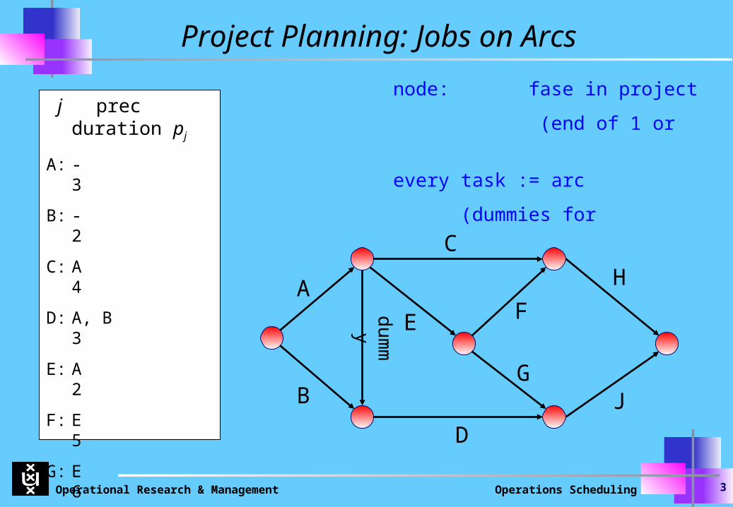
node: fase in project

(end of 1 or more tasks)

every task := arc

(dummies for precedence)

Project Planning: Jobs on Arcs

A

B

D

C

H

JG

FEd

umm

y

j prec duration pj

A: -3

B: -2

C: A4

D: A, B3

E: A2

F: E5

G: E6

H: C, F2

J: D, G4

Finish: A to J


Critical Path Method (CPM)

ES1 = 0

ESj = maxi { pi + ESi | i P(j)}

1

2

3

4

6

5

7

A 3

B 2

C 4

H 2

J 4

G 6

F 5E 2d

umm

y

D 3

0

3

3

10

5

11

15 15

11

13

5

3

0

8

j prec

A: -

B: -

C: A

D: A, B

E: A

F: E

G: E

H: C, F

J: D, G

LFn = ESn

LFi = minj { LFj - pj | j Si }


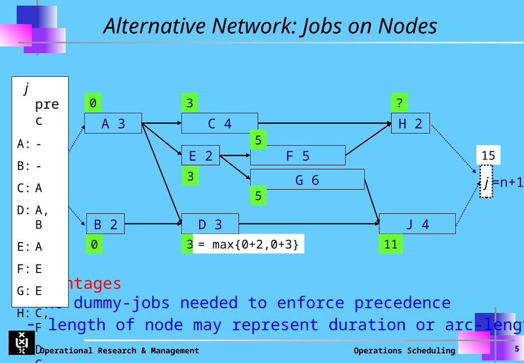
Alternative Network: Jobs on Nodes

A 3

B 2

C 4

E 2 F 5

J 4D 3

H 2

G 6

A 3

B 2

C 4

E 2 F 5

J 4D 3

H 2

G 6

3

3

3

5

5

?

11

0

0 = max{0+2,0+3}

j =n+1j = 0

150

Advantages- no dummy-jobs needed to enforce precedence- length of node may represent duration or arc-length

j prec

A: -

B: -

C: A

D: A, B

E: A

F: E

G: E

H: C, F

J: D, G


Jobs on a time axis

A 3

B 2

C 4

E 2

F 5

J 4

D 3

H 2

G 6

0 3 5 11 15 t

jobs

j prec

A: -

B: -

C: A

D: A, B

E: A

F: E

G: E

H: C, F

J: D, G


Project Planning with crashing

Heuristic

0

1 5

6

8

n+1

Graph of all Critical Path(s)

cut set

minimal cut set

4

6

4 5

6


Topic 2

Resource Constrained Project Scheduling

Problem (RCPSP)


Project Planning as Scheduling

Activities within project are jobs

Criterium: makespan onder volgorde- (en resource-restricties?)

P | prec (, rjk, Rk ) | Cmax

CPM-solution assumes: always enough resources

RCSP notation/assumptions:

Job j uses rj k units of resource k, during pj periods

Renewable resources: At any time one has Rk of resource k available

Determine all finish times Fj (=genoeg om hele schedule weer te geven)


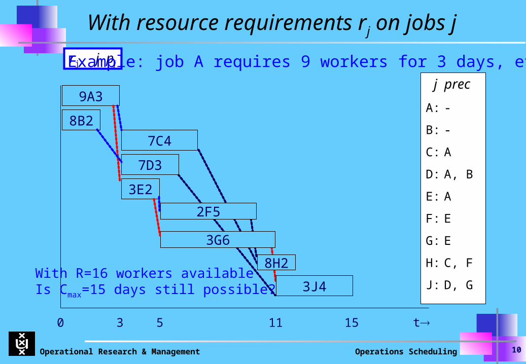
With resource requirements rj on jobs j

9A3

8B2

7C4

3E2

2F5

3J4

7D3

8H2

3G6

0 3 5 11 15 t

j prec

A: -

B: -

C: A

D: A, B

E: A

F: E

G: E

H: C, F

J: D, G

rj j pj Example: job A requires 9 workers for 3 days, etc.

With R=16 workers availableIs Cmax=15 days still possible?


With resource requirements rj on jobs j

9A3

3E2

2F5

3J4

7D3

8H2

3G6

0 3 5 11 15 t

j P(j)

A: { }

B: { }

C: {A}

D: {A, B}

E: {A}

F: {E}

G: {E}

H: {C, F}

J: {D, G}

8B2

7C4

rj j pj

Feasible, even with 12 workers


CPM on (resource-relaxed) RSCP

Generates “earliest” start- ESj and “latest” LFj finish times

The CPM-time is lower bound on RSCP-time: LFn+1 Cmax

Critical path jobs must start at ESj to accomplish Cmax = LFn+1

Other jobs have “slack”

– Their start time is NOT fixed by CPM

– Shift non-critical j in [ESj , LFj] smoothing the use of resources: after resource loading, balancing resource requirements

– If capacity Rk is still exceeded, then lengthen makespan

(let Fj exceed LFj for some j ).

Later, we discuss heuristic methods for RCPSP


Resource loading and leveling

B

7A

10

D

13

19

C

C

DE

F

ED

loading: jobs start at ESj

leveling: shift jobs in time


Conceptual Model Notation

– Decision variable: Fj (finish time) for j J

– P(j) = set of predecessors of job j

– A(t) set of active jobs j in period t

Model

Min Fn+1

s.t. Fh Fj - pj j J, hP(j)

Fj 0 j J

jA(t) rjk Rk resources k , t

A(t) = { j | Fj – pj < t Fj } t


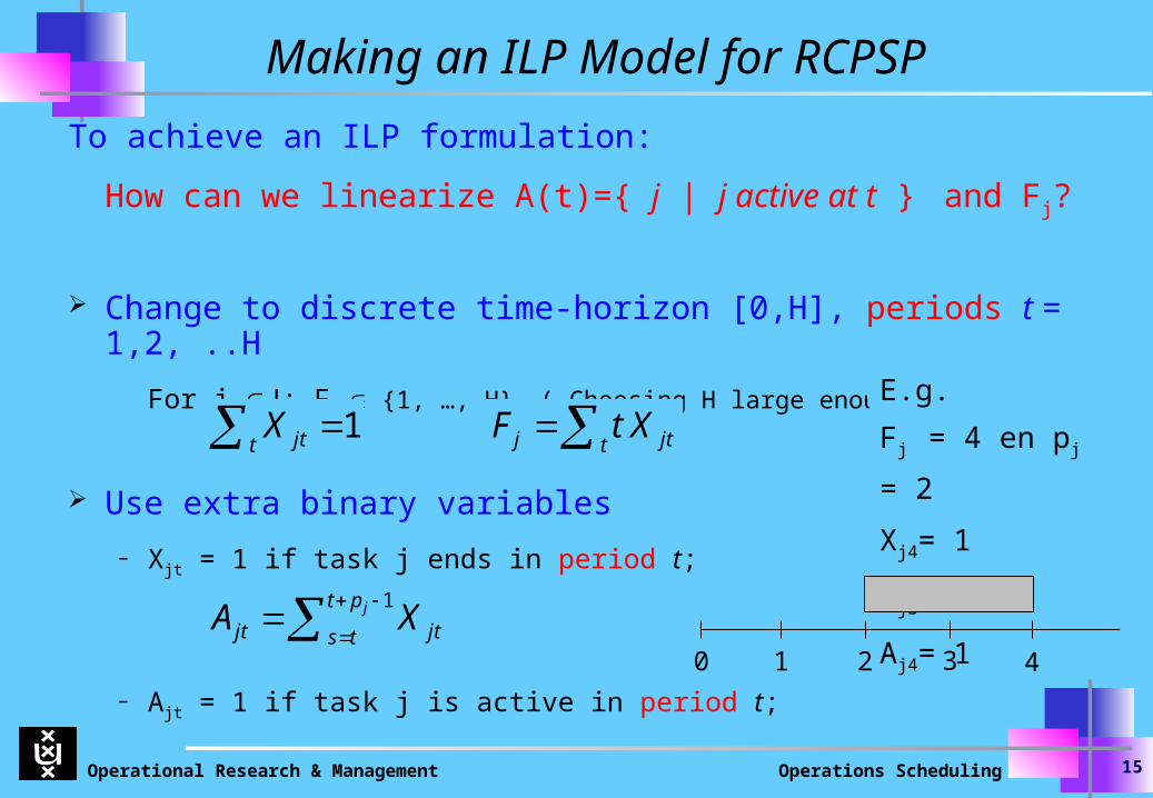
To achieve an ILP formulation:

How can we linearize A(t)={ j | j active at t } and Fj?

Change to discrete time-horizon [0,H], periods t = 1,2, ..H

For j J: Fj {1, …, H} ( Choosing H large enough)

Use extra binary variables

– Xjt = 1 if task j ends in period t;

– Ajt = 1 if task j is active in period t;

Making an ILP Model for RCPSP

j jttF t X1jtt

X

1jt p

jt jts tA X

E.g.

Fj = 4 en pj = 2

Xj4= 1

Aj3= 1 Aj4= 1

43210


Resulting ILP model for RCPSP

Min

s.t. (1) j J, hP(j)

Precedence restrictions

(2) j J

(3) j J

Determine one last period

(4) j J, t = 1, …, H

Determining active periods of tasks

(5) t = 1, …, H, k K

Consumption of scarce resources

1jt p

jt jts tA X

1

j jtt

jtt

F t X

X

h j jF F p

jt jk kjA r R

1nF


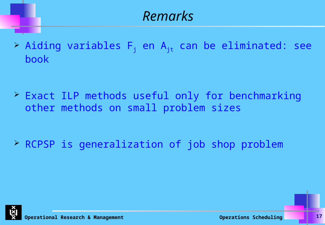
Remarks

Aiding variables Fj en Ajt can be eliminated: see book

Exact ILP methods useful only for benchmarking other methods on small problem sizes

RCPSP is generalization of job shop problem


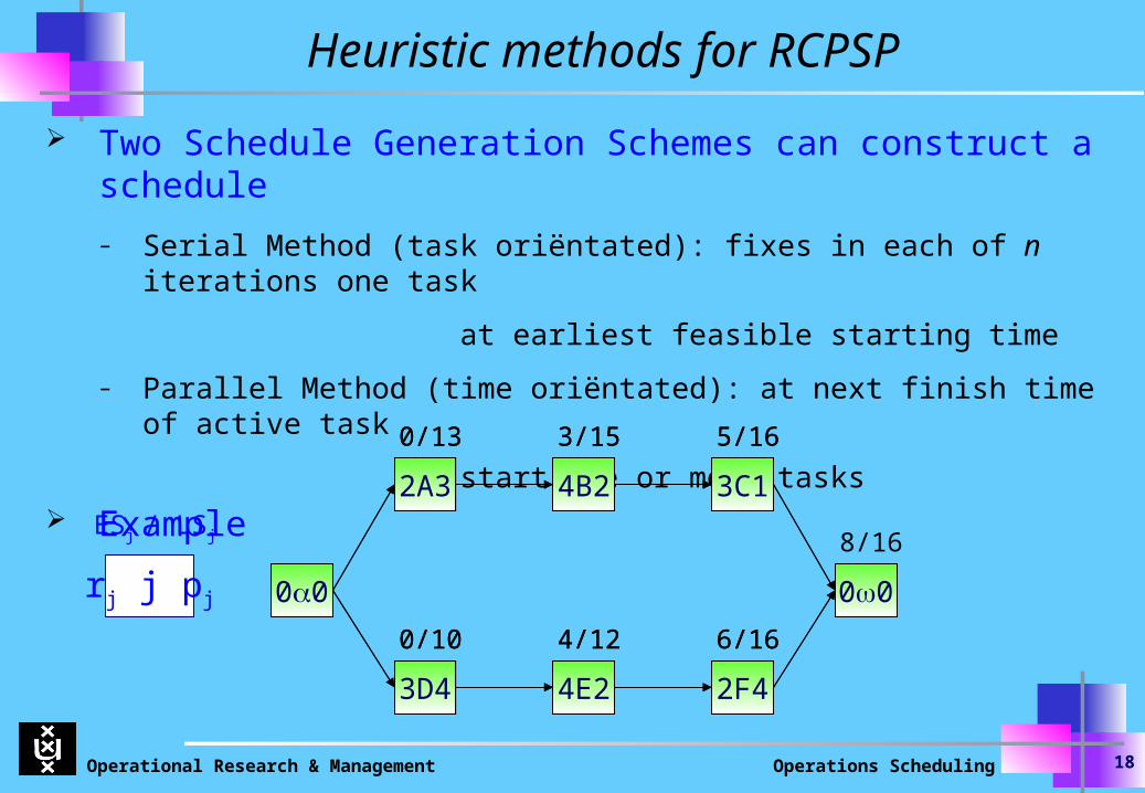
Heuristic methods for RCPSP

Two Schedule Generation Schemes can construct a schedule

– Serial Method (task oriëntated): fixes in each of n iterations one task

at earliest feasible starting time

– Parallel Method (time oriëntated): at next finish time of active task

start one or more tasks Example

00

2A3 4B2 3C1

3D4 4E2 2F4

00

0/13 3/15 5/16

4/120/10 6/16

rj j pj 00

2A3 4B2 3C1

3D4 4E2 2F4

00

0/13 3/15 5/16

4/120/10 6/16

ESj / LSj 8/16


Parallel SGS (informal)

At most n stages

Each stage g <= n represents:

1. Schedule time tg (=next finish time of scheduled job)

2. A partial schedule, consisting of four disjoint sets of jobs:

– Completed, scheduled jobs at time tg

– Active jobs: scheduled jobs, not yet completed at time tg

– Decidable jobs: unscheduled, schedulable jobs (that can be chosen to start at time tn)

– remaining set: unscheduled jobs that cannot start at time tn


Parallel SGS (on example)

tg finished R(tg) schedulable Dg j select R(tg) Fj

0 4 {A, D} 3D4 1 4 (3D)

{} - (* not A,E ; both require > 1 *)

4 3D 4 {2A3, 4E2} 4E2 0 6 (4E)

6 4E 4 {2A3, 2F4} 2A3 2 9 (2A)

{F} 2F4 0 10 (2F)

9 2A 2 { }({B}) - (* 2 short for B *)

10 2F 4 {B} 4B2 0 12 (4B)

12 4B 4 {C} 3C1 1 13


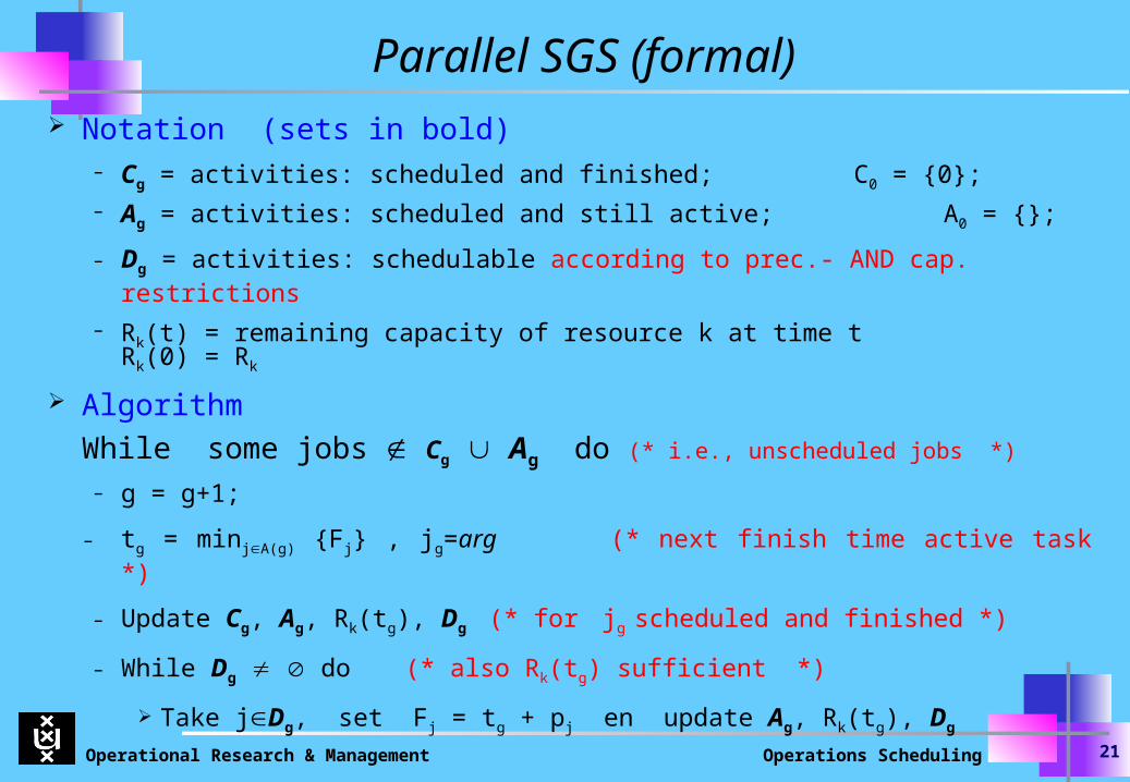
Parallel SGS (formal) Notation (sets in bold)

– Cg = activities: scheduled and finished; C0 = {0}; – Ag = activities: scheduled and still active; A0 = {};

– Dg = activities: schedulable according to prec.- AND cap. restrictions

– Rk(t) = remaining capacity of resource k at time t Rk(0) = Rk

Algorithm

While some jobs Cg Ag do (* i.e., unscheduled jobs *) – g = g+1;

– tg = minjA(g) {Fj} , jg=arg (* next finish time active task *)

– Update Cg, Ag, Rk(tg), Dg (* for jg scheduled and finished *)

– While Dg do (* also Rk(tg) sufficient *)

Take jDg, set Fj = tg + pj en update Ag, Rk(tg), Dg


Serial SGS (informal)

Each stage selects a job n stages

set of jobs already selected and planned: scheduled jobs (S )

decision set (D ): jobs with all predecessors in S

remaining set of jobs: these will first enter D and then S

Procedure

1. Start with scheduled set S=empty; j=0

2. Add j to S; Update schedulable set D ( := {j | P(j) S} );

3. Select job j from decision set D (with highest priority), and

(using {t/R(t) : finish times t } ) set j’s start/finish time as early as possible;

4. If |S|<n then go to step 2 (otherwise be happy with an 'active schedule')


Serial SGS (on example)

step { t / R(t) | t in Fg } Dg rj j pj Sj Fj updates t / R(t)

0. {0/4} {A, D} 3 D 4 0 4 R(0)=1, R(4)=4

(e.g. as priority rule: D has lower slack 8=10-(0+2))

1. {0/1,4/4} {A, E} 4 E 2 4 6 R(4)=2, R(6)=4

(idem, E has lower slack)

2. {0/1,4/2,6/4} {A, F} 2 A 3 6 9 R(6)=2, R(9)=4

(idem)

4. {0/1,4/2,6/2,9/4} {B, F} 4 F 2 6 10 R(6)=0, R(9)=2, R(10)=4

(idem)

5. {0/1,4/2,6/0,9/2,10/4} {B}4 B 2 10 12 R(10)=0, R(12)=4

6. {.. 10/0, 12/4} {C} 3 C 1 12 13 R(12)=1

Sj =min {t Fg | t ESj and k, t’ [t, t+pj) Fg : Rk(t’) rj }


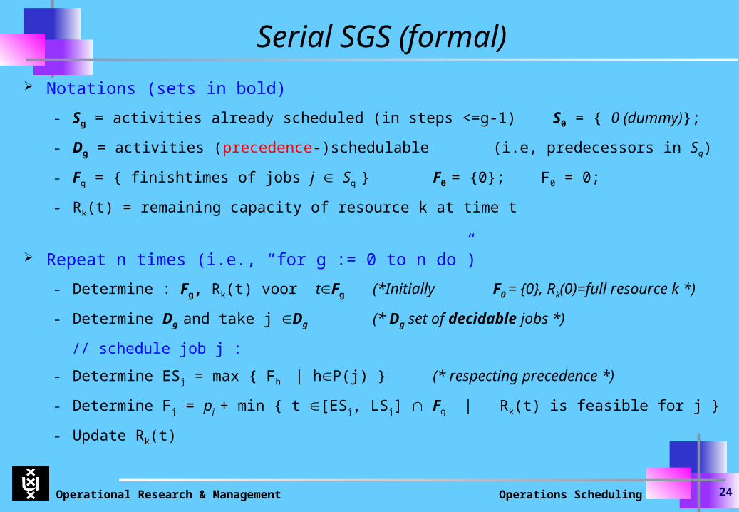
Serial SGS (formal)

Notations (sets in bold)

– Sg = activities already scheduled (in steps <=g-1) S0 = { 0 (dummy)};

– Dg = activities (precedence-)schedulable (i.e, predecessors in Sg)

– Fg = { finishtimes of jobs j Sg } F0 = {0}; F0 = 0;

– Rk(t) = remaining capacity of resource k at time t

Repeat n times (i.e., “for g := 0 to n do”)

– Determine : Fg, Rk(t) voor tFg (*Initially F0 = {0}, Rk(0)=full resource k *)

– Determine Dg and take j Dg (* Dg set of decidable jobs *)

// schedule job j :

– Determine ESj = max { Fh | hP(j) } (* respecting precedence *)

– Determine Fj = pj + min { t [ESj, LSj] Fg | Rk(t) is feasible for j }

– Update Rk(t)


Comments on Serial SGS

Constructs a feasible schedule

When resources are ample: schedule is optimal

Leads to schedule in class of ‘active schedules’,

– I.e., no operation can be earlier without others finishing later

– Class of ‘active schedules’ contains an optimal schedule

One can specify selection in “Take j in Dg” by giving:

– priority rule(s)

– an a priori list // and this explais the name ‘list scheduling’


Comments on Parallel Method

Algorithm (informal)

1. Start with finish time of active job 0 (scheduled with finish time 0)

2. In step g: tg = earliest time (that unscheduled jobs may start.)

and Dg = collection of jobs that may start at time tg

Normally, when Dg empty: tg = first finish time of active job j

3. Select the job from D with the highest priority, let it start at time tg

4. If jobs are still unscheduled then goto step 2

else stop


Comments on Parallel SGS

If ample resources then schedule is optimal

Schedule will be a non-delay schedule:

– Exercise: why is that so?

– Class of ‘Non-Delay schedules’ contains not always an optimal schedule

For serial en parallel:

– Single pass: 1 SGS combined with one Priority Rule

– Multi pass

1 SGS with all PR’s

Forward-backward scheduling

Sampling method: “random”, “biased” or “regret based biased”

Metaheuristics


Topic 3

Parallel Machine Scheduling Problems


Parallel Machine Models

Lets say we have

– Multiple machines (m), where

– the makespan should be minimized (Cmax)

We denote this problem as

Problem already NP-hard for m = 2 (partitioning problem)

LPT-rule good heuristic

max||Pm C


Worst case behaviour LPT

Maximal deviation from optimal value

Example: four parallel machines, nine jobs

Cmax(opt)=12 but Cmax(LPT)=15

max

max

( ) 4 1

( ) 3 3

C LPT

C OPT m

jobs 1 2 3 4 5 6 7 8 9p ( j ) 7 7 6 6 5 5 4 4 4


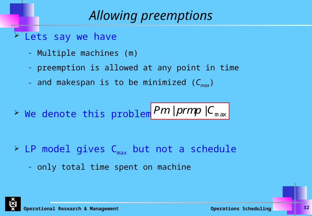
Allowing preemptions Lets say we have

– Multiple machines (m)

– preemption is allowed at any point in time

– and makespan is to be minimized (Cmax)


LP model gives Cmax but not a schedule

– only total time spent on machine

max| |Pm prmp C


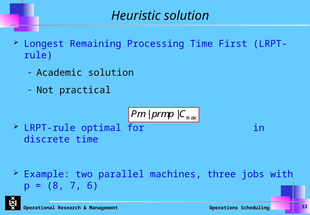
Heuristic solution

Longest Remaining Processing Time First (LRPT-rule)

– Academic solution

– Not practical

LRPT-rule optimal for in discrete time

Example: two parallel machines, three jobs with p = (8, 7, 6)

max| |Pm prmp C


One final model

Lets say we have

– Multiple machines (m), where

– the total completion time should be minimized (Cj)


SPT-rule gives optimal schedule

For the weighted case: WSPT does not give optimal schedule

|| jPm C

operational research & managementoperations scheduling project scheduling 1.project planning...

Documents