Operating Leverage over the Business Cycle

Arnab Bhattacharjee, Heriot Watt University. A.Bhattacharjee@hw.ac.ukChris Higson, London Business School. CHigson@london.eduSean Holly, University of Cambridge. sh247@cam.ac.uk

Janaury 2016

Abstract

Operating leverage describes the extent to which a firm’s operating costs arefixed in the short run. The effect of operating leverage is to amplify the impacton profit of a change in revenues; an effect which is further amplified by financialleverage and by asymmetry in the tax system. In this paper we provide empiricalestimates of operating leverage at the firm level, using a long panel of data onUK quoted firms. We report sectoral differences in operating leverage around thebusiness cycle, and show that these can be partly explained in terms of costly labouradjustment and asymmetric price adjustment.

1

Operating Leverage over the Business Cycle

January 2016

Abstract

Operating leverage describes the extent to which a �rm�s operating costs are�xed in the short run. The e¤ect of operating leverage is to amplify the impacton pro�t of a change in revenues; an e¤ect which is further ampli�ed by �nancialleverage and by asymmetry in the tax system. In this paper we provide empiricalestimates of operating leverage at the �rm level, using a long panel of data onUK quoted �rms. We report sectoral di¤erences in operating leverage around thebusiness cycle, and show that these can be partly explained in terms of costly labouradjustment and asymmetric price adjustment.

JEL Classi�cation: E32, D4, G30.

Keywords: operating margin, panel data, �xed and �exible costs, business cycles.

1

I. Introduction

Operating leverage describes the extent to which a �rm�s operating costs are �xed in theshort run. If the �rm cannot, or chooses not to, fully adjust costs when revenues change,this is directly observable in operating pro�t margins. The operating leverage e¤ectof a change in revenues on earnings is ampli�ed by underlying business risk, �nancialleverage and by asymmetry in the tax system (Hamada (1972), Rubinstein (1973), Lev(1974), Bowman (1979), Mandelker and Rhee (1984), Mensah (1992)). Hence, operatingleverage lies at the heart of the distinction between cyclical and non-cyclical �rms in�nancial markets.One reason for the concern with operating leverage in the �nance literature is its

potential to explain the value premium; the observation that �value� stocks with highbook-to-market ratios earn higher returns than growth stocks (Carlson et al. (2004),Zhang (2005) and Cooper (2006)). Value �rms earn higher returns because they largelyuse assets in place that are riskier than growth options because of operating leverage;without operating leverage growth options are riskier than assets in place (Lev, 1974;Novy-Marx, 2011), so the value premium re�ects the �rm�s investment behaviour (Famaand French, 1996; Chen and Zhang, 1998; Berk et al., 1999). In Fama and French (1996)the value premium compensates for �nancial distress risk, with potentially negative e¤ectson intangible elements of wealth such as human capital.Garc¬a-Feijoo and Jorgensen (2010) report that the book-to-market ratio, beta, and

average stock returns are all positively associated with the degree of operating leverage inthe cross-section. In Gulen et al. (2008) value �rms have higher operating leverage, higher�xed to total asset ratios, greater frequency of disinvestment, and higher �nancial leveragethan growth �rms, and are less �exible than growth �rms in adjusting to worseningeconomic conditions. Other empirical studies that support a risk explanation of thevalue premium include Mandelker and Rhee (1984), Lord (1996), Ho et al. (2004) andNovy-Marx (2007). Novy-Marx1 �nds that the book to market ratio explains returnswithin an industry, though not between industries (also Zhang (2005) and Aguerrevere(2006)).Survey-based evidence in industrial economics has suggested an asymmetric response

1Unconventionally, in Novy-Marx (2007) �operating leverage�is the pro�t margin while the variation

in that margin due to sticky costs is termed �degree of operational in�exibility�(also, Gourio (2005)). He

says: �While higher variable costs result in e¤ectively more levered assets, they should also be associated

with more �exibility on the cost side. When capital costs are small relative to �ow costs associated

with production, �rms should be more willing to shut down unpro�table production, even if it entails the

loss of capital. . . . Operating leverage is, to �rst-order approximation, the inverse of a �rm�s operating

margins, and thus it is generally closer to ten than zero . . . In response to negative shocks �rms�revenues

typically fall more quickly than they can reduce costs; prices are more responsive than �rms�operations.

. . . While simple theory suggests that expected returns should be increasing in operating leverage, the fact

that they should also be increasing in operational in�exibility, which is di¢ cult to observe and negatively

correlated with the level of operating leverage, makes direct inference on the expected return/operating

leverage relationship di¢ cult.�

2

to a shock to sales, with quantity adjustments more likely in recessions than in booms(Machin et al. (1993)). Liquidity constrained �rms are less likely to cut prices (Gottfries(1991)), implying that additional liquidity may be more important in recessions that aredriven by demand shocks. Liquidity constraints and limited access to capital marketsmay explain the greater procyclicity of small �rms, which therefore bear the brunt ofmonetary policy shocks (Gertler and Gilchrist (1994)).Though pro�t margins are observably procyclical (Green and Porter (1984); Machin

and van Reenen (1993)), it has proven hard to extract measures of operating leveragefrom the observed behaviour of pro�t margins. For some raw materials, supply maybe rapidly adjustable and reversible at little cost. Highly speci�c plant and equipmentmay be hard to sell and di¢ cult to reacquire; it may trade in illiquid markets witha wide spread between disposal value and replacement cost. Campello and Giambona(2013) and James and Kizilaslan (2014) argue that only those tangible assets that can beeasily redeployed can sustain debt capacity. In this way, operating leverage and �nancialleverage may be natural substitutes. In Acharya, Almeida and Campello (2013) �rmswith high asset betas hold more cash and have a higher cost of debt �nancing.The adjustment of physical capital and human capital go hand-in-hand as they are

the two key dimensions of capacity. Skilled labour has the character of speci�c industrialplant. Employment law and labour contracting create lags in the adjustment of labourinputs so that, on the downside, a labour-cost response may be observed signi�cantlylater than a fall in revenue. On the upside, labour may be costly to acquire or reacquireand can take both time and expenditure to equip it with organization speci�c knowledge.As with speci�c intangible assets, the replacement cost of skilled labour is likely to moveprocyclically.For labour cost, �rms disclose both employment and wage but, otherwise,the price and quantity components of cost and revenue are not observable in panel data.One thing that makes operating leverage empirically elusive is the role of expectations

where there are asymmetric adjustment costs to increasing and reducing capacity. If a�rm or an industry is undergoing secular growth or contraction that is fully anticipatedthen capacity can be adjusted and even ��xed assets�, physical capital, can be bought orsold in a timely way. In practice, �rms may be slow to recognise secular growth or declineor slow to respond to it, especially if they are uncertain whether it will be temporaryor permanent. If the �rm faces what it believes to be a cyclical change in demand andif adjustment is costly then it may be rational to maintain unused capacity through thecycle. At an in�ection point, �rms may be unclear whether a change in revenues is secularor cyclical and how long the cycle will last.We have the following testable predictions:

� We predict that small �rms experience greater costs of adjusting capacity and,assuming size proxies �nancial strength, large �rms are better able to bear thecosts of non-adjustment. We measure size both in terms of employment and thequantity of �xed capital.

� We predict that adjustment costs may be asymmetric, so that �rms exhibit higheroperating leverage, that is the non-adjustment of capacity leading to relativelydepressed margins, in cyclical downturns than in upturns.

� Asymmetric response of costs may also re�ect price adjustments over the economiccycle, rather than quantity adjustments, where such adjustments are subject tonominal rigidities (Machin et al. (1993)).

3

� Since the costs of adjusting capacity are likely to re�ect the nature of the inputs,we expect to see systematic di¤erences in cyclicity between sectors.

We estimate a model of operating leverage by applying panel data methods to dataon UK quoted �rms from 1968 to 2011. Much of the data displays temporal non-stationarity and potentially strong dependence cross-sectionally (Petersen (2009)). Thiscross-sectional dependence is related to factor structure that needs to be modelled explic-itly (Fama and French (1992, 1996); Gri¢ n (2002)). We address these issues as follows.To allow for nonstationarity of our main activity measures, sales and costs at the

�rm-level (in logarithms), we model the relationship between costs and sales (operatingleverage) as a dynamic, non-stationary process. We allow that sales and costs maybe in long-run equilibrium so that, at the �rm-level, logarithms of sales and costs arepotentially cointegrated. The short-run and long-run dynamics between costs and salesis modelled as an error correction process in which the underlying series are non-stationaryand potentially cointegrating. Cross-section dependence is modelled using the commoncorrelated e¤ects approach of Pesaran (2006), which allows for potential factor-basedstrong dependence. This powerful framework allows us the determine how operatingleverage reacts, in the short run, to variations in the use of capital and employment, andalso the extent to which there is asymmetric adjustment.In section 2 we describe the data. In section 3 we develop and estimate a model of

operating leverage and in section 4 we draw conclusions.

II. Data and descriptives

The data are drawn from the LBS/Cambridge accounting data set, which is an archiveof annual company balance sheet and income statement data for all UK industrial andcommercial quoted companies. In terms of coverage, the dataset attempts to be completein companies listed on a UK exchange, principally the London Stock Exchange and alsothe junior markets including USM (Unlisted Securities Market) and AIM (AlternativeInvestments Market). We include industrial and commercial companies, but exclude�nancial and property companies. There is substantial attrition in the population oflisted �rms as �rms exit through acquisition or failure, and enter through stock exchangelisting. Hence, the panel is unbalanced but large. The dataset contains between 1500and 2000 companies per annum. Since UK companies were required to disclose sales forthe �rst time in 1967, 1968 is the �rst year with a measure of sales growth. The sectoralcomposition is described in Table 1 (top panel: 1968 to 1989; bottom panel: 1990 to2010).Certain features of �rm panel data add measurement error and confound our ability

to interpret the results. Some companies are exporters and some are multinational inoperation so that their data includes the results of foreign operations, reducing the po-tential alignment between reported sales of these companies and domestic GDP. Equally,foreign-owned domestic �rms are missing from the data, although their output forms partof domestic GDP. Data are drawn from annual �nancial statements with heterogeneousaccounting year ends �in this data 37% of companies have a December year-end; March,22%; September, 10%; June, 8%. Our convention is to assign observations to the previouscalendar year when the �nancial statement date is 19 May or before.

4

1

1:pdf

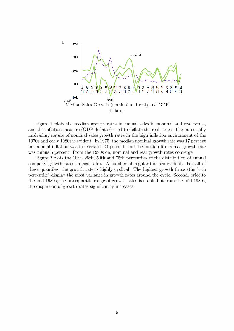
Median Sales Growth (nominal and real) and GDPde�ator.

Figure 1 plots the median growth rates in annual sales in nominal and real terms,and the in�ation measure (GDP de�ator) used to de�ate the real series. The potentiallymisleading nature of nominal sales growth rates in the high in�ation environment of the1970s and early 1980s is evident. In 1975, the median nominal growth rate was 17 percentbut annual in�ation was in excess of 20 percent, and the median �rm�s real growth ratewas minus 6 percent. From the 1990s on, nominal and real growth rates converge.Figure 2 plots the 10th, 25th, 50th and 75th percentiles of the distribution of annual

company growth rates in real sales. A number of regularities are evident. For all ofthese quantiles, the growth rate is highly cyclical. The highest growth �rms (the 75thpercentile) display the most variance in growth rates around the cycle. Second, prior tothe mid-1980s, the interquartile range of growth rates is stable but from the mid-1980s,the dispersion of growth rates signi�cantly increases.

5

Table 1. Sector (1-; 2- digit) composition of the sample:

1a

2:pdf

1b

3:pdf

Third, in any year a signi�cant proportion of the corporate population do not growand have real sales that are either �at or declining. Fourth, the median growth rate inreal sales is stationary throughout this 40 year period at only slightly above zero. Fifth,negative real growth is the norm at the �rst quartile. Real growth at this quantile is neverpositive; even in boom periods it may reach but does not exceed the zero axis. Finally,during the deepest downturn during this 40 year period, which was the 1980s recession,even at the third quartile (75th percentile) growth of zero. At that time, 75 percent of�rms experienced negative real growth.Table 2 reports median annual real sales growth rates by one-digit and two-digit

industry sectors. For reference the table also reports the percentage annual change inreal GDP (O¢ ce of National Statistics (ONS) data series IHYP). We want to observehow individual company fundamentals (sales, costs, pro�ts) move around the businesscycle. Using sales as the measure of a �rm�s activity and aggregate GDP to proxy the

6

2

4:pdf

Figure 1: Distribution of company growth rates (selected percentiles)

average response, we examine the dynamics of activity, taking into account heterogeneityacross sectors in their relation to the aggregate cycle. We expect to �nd that sectorsmay lag or lead the aggregate economy in the response to a downturn, and may displaya greater or smaller response, or in some cases no response at all.Table 2 �ags recessionary years, that is, calendar years experiencing negative growth

rate in aggregate GDP. Although there is substantial alignment between sector salesgrowth and change in aggregate GDP, the disaggregate analysis points to variations inthe experience of �rms during di¤erent episodes of downturn. For example, the deep1980-1981 recession in the observed in aggregate data was also associated with decliningreal sales in almost all sectors. However, most sectors also reported negative sales growthin 1979 and in 5 of 18 sectors there was a fourth year of negative sales growth in 1982.There was a similar, though less intense, pattern around the 1991 downturn, with 6 sectorsreporting sales downturn in 1990. The recession that followed the recent �nancial crisis isoften described as the deepest in living memory. The 2009 recession was uniquely sharpin terms of the decline in GDP. But for the �industrial�economy that we are examining inthis paper, with the notable exception of construction the impact of recession was bothsmaller, and less consistent across sectors, than in the 1980-1981 downturn. Table 1b also�ags the �quasi recessionary�year, 2002. In terms of the impact on median sales growththis was a worse year than 2009 in many sectors. However this is not equally re�ected inaggregate GDP.Figure 3 plots the median return on capital employed (pro�t/capital employed), where

capital employed is the sum of equity shareholders� funds and long- plus short-termborrowing less cash. Pro�t is earnings before interest and tax, depreciation, amortisationand impairment, and exceptional items. For comparison, the dotted line in Figure 3 isthe median real sales growth series from Figure 1. It is clear that most, though not all,of the time series variation (cyclicity) in real sales growth is re�ected in return on capitalemployed.

7

Table 2. Cyclicity of company growth at the sector level:

2a

5:pdf

2b

6:pdf

Figure 3 then decomposes the return on capital employed into its pro�t margin(pro�t/sales) and asset utilisation (sales/capital employed, right hand axis) components.Apparently, most of the variation in return on capital employed is coming from sales.Pro�t margins are procyclical, but pro�t margins display a dampened response to shocksto sales, suggesting that there is some pass through to costs. At the same time, the pass-through is not perfect, otherwise pro�t margins would not exhibit the cyclical pattern

8

3

7:pdf

Figure 2: Components of returns, 1968 �2010.

observed in the data.

Table 3. E�ect of the cycle on the median margin at the sector level:

3a

8:pdf

3b

9:pdf

9

Table 3 reports the median annual pro�t margin by (1 digit and 2 digit) sector.Broadly, the data display some compression in pro�t margins in economic downturns,however the story is a complex one. Some industries, for example oil and gas, displayedtemporal patterns in margins that are apparently unconnected to the aggregate businesscycle, while margins in other industries appear to have responded more strongly to somedownturns than to others.Geroski and Gregg (1998) focused on two major UK recessions, which they dated

1980-1981 and 1990-1991. They concluded that the recession caused a sea change inpro�t margins that, having fallen in recession, never fully recovered. Inspection of Table3 o¤ers some limited evidence of this. At least in some sectors, the fall in margin persistedfor a number of years beyond the �recessionary�period.The sector medians reported in Table 3 need to be interpreted with caution. As seen

in Table 1, some of these sectors are thinly populated in some years, so that the mediansare maybe unrepresentative. For instance, although the automobile industry accountsfor a signi�cant proportion of UK GDP, since 1990 the major UK automobile companies(assemblers) are foreign-owned and are thus missing from our data.

III. A basic model of operating leverage

In the corporate �nance literature, papers (for example, Ang and Peterson (1984); DeY-oung and Roland (2001); Gri¢ n and Dugan (2003); Ho et al. (2004)) commonly employsome variant of the approach in Mandelker and Rhee (1984), who estimate the �degree ofoperating leverage�, DOL, as the slope coe¢ cient in a time-series regression of pro�t, orcosts, on sales. Other researchers proxy operating leverage as a �nancial ratio such as theratio of �xed assets to total assets (Ferri and Jones, (1979); Lord (1998)). In Novy-Marx(2007) �operating leverage�is the pro�t margin while the variation in that margin dueto sticky costs is termed �degree of operational in�exibility�(also Gourio (2005))2. Thisapproach, that uses average pro�t margin as a proxy for operating leverage can at bestonly indirectly capture the notion of operating leverage, as it is popularily used, and inits role as a risk factor in theories of the risk premium. That is a story about changesin margin in response to a shock to sales and about the determinants of the stickiness incosts. Studies that regress the logarithm of operating costs on the logarithm of sales anduse the coe¢ cient on sales to measure operating leverage come closer to examining the

2He says: �While higher variable costs result in e¤ectively more levered assets, they should also be

associated with more �exibility on the cost side. When capital costs are small relative to �ow costs

associated with production, �rms should be more willing to shut down unpro�table production, even if

it entails the loss of capital. . . . Operating leverage is, to �rst-order approximation, the inverse of a

�rm�s operating margins, and thus it is generally closer to ten than zero . . . In response to negative

shocks �rms�revenues typically fall more quickly than they can reduce costs; prices are more responsive

than �rms� operations. . . . While simple theory suggests that expected returns should be increasing in

operating leverage, the fact that they should also be increasing in operational in�exibility, which is di¢ cult

to observe and negatively correlated with the level of operating leverage, makes direct inference on the

expected return/operating leverage relationship di¢ cult.�

10

issues (Lev (1974) is an early example and Kahl et al. (2013) a recent one.Machin and van Reenen (1993) regress the change in pro�t margin on the business

cycle, proxied by the unemployment rate, allowing for �rm-level controls and dynamics.Their sample is larger UK �rms over the 1970s and 1980s, covering one major recession- the early 1980s. They �nd that the pro�t margin is stationary and cyclical. Marginsdecline sharply in recessions, though the timing of the impact of aggregate shocks appearsto di¤er across sectors.We draw upon a number of recent developments in panel data and spatial econometrics

to estimate a panel error correction model. We �rst estimate the model using conventionalpanel methods where slopes are homogeneous and possible cross sectional correlation isignored. Next, we model potential heterogeneity caused by slope coe¢ cients varyingacross �rms using the mean group estimator of Pesaran and Smith (1995). This methodinvolves �rst separately estimating a time series error correction model for each crosssection unit. Next, under the assumption of random slope coe¢ cients (Swamy (1970)),the mean slope is estimated as the average of these cross-section speci�c slope estimates;the standard error is also estimated in a similar way. If a test that the slope estimates forthe long run e¤ect are actually the same across �rms is not rejected, we use the pooledmean group estimator (Pesaran et al., 1999).To allow for nonstationarity of our main activity measures, sales and costs at the

�rm-level (in logarithms), we model the relationship between costs and sales (operatingleverage) as a dynamic, non-stationary process. In doing so, we admit the possibilitythat sales and costs may be in long-run equilibrium. In other words, at the �rm-level,logarithms of sales and costs are potentially cointegrated. Importantly, this frameworkallows us the determine how operating leverage reacts, in the short run, to variations inthe use of capital and employment, and also the extent to which there is asymmetric ad-justment. The short-run and long-run dynamics between costs and sales is modelled as anerror correction process in which the underlying series are non-stationary and potentiallycointegrating. Cross-section dependence is modelled using the common correlated e¤ectsapproach of Pesaran (2006), which allows for potential factor-based strong dependence.The �rst model we work with is a �xed e¤ects panel error correction model with

homogeneous slopes,

� ln cit = �i + �� ln sit � (ln ci;t�1 � � ln si;t�1) + "it; i = 1; N; t = 1; T: (1)

Here cit and sit denote the costs and sales of �rm i in year t. The form of the modelallows us to treat the determination of the change in margin, � ln(cit=sit), simultane-ously with the margin itself, ln(cit=sit). The model includes �rm-speci�c �xed e¤ects �icapturing unobserved �rm-level heterogeneity, including the hazard rates (Mill�s ratio) ofattrition from the sample. Hence, potential sample selection bias is accounted for. Therelationship between costs and sales includes partial adjustment ( ) to a hypothesizedlong run equilibrium relationship between log-costs and log-sales, the e¤ect of sales oncosts in long-run equilibrium (�), and the short-run dynamic e¤ect of sales on costs (�).Speci�ed this way, if � � 1, (ln cit � �i ln sit) � ln (1� �it), where �it denotes the

pro�t margin of �rm i in year t. We test the stationarity of ln (1� �it), and test for ahomogeneous long run equilibrium, implying that �i = �; with, in the limit, � = 1. In suchan equilibrium, the value of ln (1� �it) is ��i= i and the �rm would anticipate partialadjustment of (ln ci;t�1 � � ln si;t�1) to this equilibrium.The short-run �rm-speci�c slope coe¢ cient � captures the e¤ect of a shock to sales �

our estimate of operating leverage. If a �rm can pass a shock to sales completely through

11

to costs, margin stays unchanged, so � = 1. If pass-through is incomplete, E (�) < 1.We test H0 : E (�) = 1 against the left-tailed alternative H1 : E (�) < 1. We start withan analysis of the basic statistical properties of our �rm-level data.

A. Stationarity and cointegration

We have a large, very unbalanced data set so the power of the tests for panel unit rootscan have low power when the number of observations are small. Table 4 reports panelunit root tests for a more limited set using the Im-Pesaran-Shin test (Im et al., 2003),when there are at least 20 and 30 complete observations for each �rm. Heterogeneityacross �rms in the slope (autoregressive parameter) is allowed. The null hypothesis isthat all �rms have unit roots against the alternative that a �nite proportion of �rms havestationary sales (or costs).

Table 4: Panel Unit Root Tests

Observations >20 >30Firms 849 373Average years 30.5 37.4lnCosts 0.380y 0.941y

lnSales 0.025y 0.436y

�lnCosts 0.000y 0.000y

�lnSales 0.000y 0.000yy p-values

The null that all �rms in the panel have unit roots for both real sales and real costs (inlogarithms) is not rejected at the 1% level. However, the unit root hypothesis is rejectedfor growth in real sales and real costs. Thus,

ln sit; ln cit � I(1);

where sit and cit denote real sales and real costs respectively, for �rm i in year t.Given that sales and costs have unit roots the next question is whether sales and costs

are cointegrated and that there is a proportionate relationship between costs and sales,so that the pro�t margin in the long run is stationary. An indirect test of cointegration(Stock, 1987 and Stock and Watson, 1993) is whether the non-stationary terms in the logof sales and costs are statistically signi�cant in a regression of the (stationary) change inthe log of costs. This test is reported in Table 5. In all cases both terms are signi�cantlydi¤erent from zero. A joint test for whether the two coe¢ cients are zero ( = � = 0) isalso rejected.The coe¢ cient on � ln sit in Table 5 provides a measure of whether a shock to sales

produces a proportionate change in costs. Depending upon the sample size this variesfrom 68 percent to 85 percent. A test for the null restriction that lncostst�1�lnsalest�1 =0 ( = ��) is also rejected. This suggests that when we assume both homogeneousslopes and cross sectional independence, pro�t margins are non-stationary. At the sametime, unit root tests indicate that pro�t margins are stationary. Together, this points tosubstantial heterogeneity across �rms, so that the slope homogeneity assumption may besomewhat misplaced.

12

Table 5: Tests for Cointegration

Response: � lncostst Pooled Panel, FE Panel, FE Panel, FE Panel, FEIncluded �rms all all >10 years >20 years >30 years� lnsalest 0.676*** 0.698*** 0.777*** 0.857*** 0.851***

(0.00206) (0.00211) (0.00225) (0.00231) (0.00231)lncostst�1 -0.212*** -0.500*** -0.452*** -0.417*** -0.4635***

(0.00223) (0.00359) (0.00388) (0.00492) (0.00718)lnsalest�1 0.191*** 0.438*** 0.415*** 0.405*** 0.4546***

(0.00207) (0.00337) (0.00370) (0.00484) (0.00707)Constant 0.157*** 0.425*** 0.244*** 0.0644*** 0.0364***

(0.00345) (0.00858) (0.00804) (0.00702) (0.00755)

Observations 55,330 55,330 42,931 24998 13571R-squared 0.674 0.719 0.767 0.860 0.890Number of �rms 4,901 4,901 2,147 849 373Joint Test: p-valueslncostst�1 =lnsalest�1 = 0 0.000 0.000 0.000 0.000 0.000lncostst�1�lnsalest�1 = 0 0.000 0.000 0.000 0.000 0.000Standard errors in parentheses*** p<0.01, ** p<0.05, * p<0.1Panel, FE: �xed e¤ects regression; Pooled: pooled OLS

IV. Slope Heterogeneity and Mean Group Estima-tors

An assumption in the previous section is that the estimates of the slopes in the modelare constant across �rms. We now relax the assumption of constant slopes and reportmean group estimates of the slopes in equation (1). Our basic model is now a panel errorcorrection model with heterogeneous slopes,

� ln cit = �i + �i� ln sit � i (ln ci;t�1 � �i ln si;t�1) + "it; i = 1; N; t = 1; T: (2)

In other words we estimate the model for each �rm and then take the average of the slopes(Pesaran and Smith, 1995). In the panel error correction model (1), an assumption issometimes made that the long run e¤ect is homogeneous across �rms (�i = �), while theshort run e¤ect and partial adjustment is potentially heterogeneous. The pooled meangroup estimator (Pesaran et al., 1999) can then be used. The mean group and pooledmean group estimates are shown in Tables 6a and 6b for di¤erent numbers of observationsfor each �rm.The short run e¤ects - estimates of the coe¢ cients on sales growth (� lnsales), as a

measure of operating leverage - are now around 94 to 95 percent. This is much larger andcloser to unity than the homogeneous slope estimates in Table 5. However, the di¤erencefrom unity, E (�i) = 1, is statistically signi�cant in a one tailed test, suggesting thatthere is substantial operating leverage. In response to a shock to sales, on average, costsare adjusted by 94 percent within the same year.Together, there is evidence of a cointegrating long term equilibrium relationship be-

tween logarithm of costs and sales. The partial adjustment in one year to this long-run

13

equilibrium is estimated by the mean group estimator at around 42-47 percent. Thepooled mean group estimates are statistically signi�cantly di¤erent. This is not unex-pected, since the assumption of a common long run sales-cost equilibrium across all �rmsin all the sectors may be too strong. A Hausman test (Hausman (1978)) rejects, at the1% level, the null hypothesis of a homogenous long-run coe¢ cient across all �rms. Thismay be di¤erent when we conduct sectoral analyses later in the paper. Firms within aspeci�c sector may well have in equilibrium a common sector-speci�c pro�t margin.

Table 6: Mean Group and Pooled Mean Group Estimators

6a) Firm observations>20 Mean Group Pooled Mean GroupResponse: � lncostst error correction short run error correction short runRegressorsPartial adj., : Ecmt�1 -0.466*** -0.392***

(0.00928) (0.00916)� lnsales 0.938*** 0.936***

(0.00435) (0.00418)lnsalest�1 1.064*** 1.005***

(0.0404) (0.000536)Constant -0.0507*** -0.0386***

(0.0121) (0.00151)

Observations 24,998 24,998 24,998 24,998p-valuelnsalest�1 = 1 0.111 0.000

6b) Firm Observations>30 Mean Group Pooled Mean GroupResponse: � lnCostst error correction short run error correction short runRegressorsPartial adj., : Ecmt�1 -0.418*** -0.353***

(0.0119) (0.0115)� lnsales 0.952*** 0.952***

(0.00543) (0.00536)lnsalest�1 1.014*** 1.001***

(0.00686) (0.000756)Constant -0.0372*** -0.0280***

(0.0112) (0.00131)

Observations 13,571 13,571 13,571 13,571p-valueslnsalest�1 = 1 0.0431 0.0539Standard errors in parentheses*** p<0.01, ** p<0.05, * p<0.1

V. Cross Section Dependence

Thus far we have reported results for both homogeneous and heterogeneous slopes. How-ever, the recent literature on large panels has highlighted the need to test for cross-

14

sectional strong dependence generated by latent (or unobservable) factors with loadingsthat are heterogeneous across �rms. These latent factors may generate strong cross sec-tion dependence among �rms and, if omitted from the model, may invalidate inferencesfrom panel data models. To proxy the e¤ect of potentially multiple latent factors, thecommon correlated e¤ects (CCE) method (Pesaran, 2006; Holly et al., 2011; Bailey etal., 2013) includes cross section averages of the dependent and independent variables asadditional regressors.3

Strong cross-sectional dependence comes from factors that a¤ect all cross section units,though by di¤ering amounts. An example is macroeconomic developments - if we expandthe number of cross section units, even as N ! 1, then all �rms are still a¤ected bymacroeconomic developments. Weak cross-sectional dependence is more localised. Firmsmay be correlated because they belong to the same industry which is subject to somecommon technological developments, because they belong to the same regional (spatial)area which is subject to local shocks, or through supply or demand side linkages.

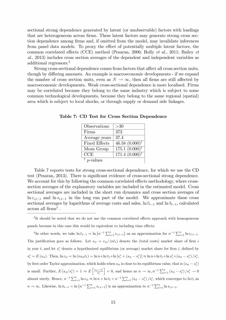
Table 7: CD Test for Cross Section Dependence

Observations >30Firms 373Average years 37.4Fixed E¤ects 46.58 (0.000)y

Mean Group 175.1 (0.000)y

CCE 171.4 (0.000)yy p-values

Table 7 reports tests for strong cross-sectional dependence, for which we use the CDtest (Pesaran, 2013). There is signi�cant evidence of cross-sectional strong dependence.We account for this by following the common correlated e¤ects methodology, where cross-section averages of the explanatory variables are included in the estimated model. Crosssectional averages are included in the short run dynamics and cross section averages ofln ci;t�1 and ln si;t�1 in the long run part of the model. We approximate these crosssectional averages by logarithms of average costs and sales, ln ct�1 and ln st�1, calculatedacross all �rms4 .

3It should be noted that we do not use the common correlated e¤ects approach with homogeneous

panels because in this case this would be equivalent to including time e¤ects.

4In other words, we take ln ct�1 = ln�n�1

Pni=1 ci;t�1

�as an approximation for n�1

Pni=1 ln ci;t�1.

The justi�cation goes as follows. Let sit = cit= (nct) denote the (total costs) market share of �rm i

in year t, and let s�i denote a hypothesized equilibrium (or average) market share for �rm i, de�ned by

s�i = E (sit). Then, ln cit = ln (nsitct) = lnn+ln ct+ln [s�i + (sit � s�i )] � lnn+ln ct+ln s�i+(sit � s�i ) =s�i ,

by �rst order Taylor approximation, which holds when sit is close to its equilibrium value, that is (sit � s�i )

is small. Further, E (sit=s�i ) = 1 ) Ehsit�s�is�i

i= 0, and hence as n ! 1; n�1

Pni=1 (sit � s�i ) =s�i ! 0

almost surely. Hence, n�1Pn

i=1 ln cit � lnn+ ln ct + n�1Pn

i=1 (sit � s�i ) =s�i , which converges to ln ct as

n!1. Likewise, ln st�1 = ln�n�1

Pni=1 si;t�1

�is an approximation to n�1

Pni=1 ln si;t�1.

15

In Table 8 we report results for the heterogeneous case using the common correlatede¤ects estimator with group mean estimates. Two cases are distinguished. The meangroup estimator in the left hand side of the table reports cross sectional averages of allof the parameters in equation (1). The pooled mean group estimates in the right handside of the table still take the cross sectional averages of the estimates of � lnsalest (andin general any estimates of the short run part of the equation) but the coe¢ cients on thelong run part, impose (and test for) a common set of coe¢ cients.As with the results in Table 5 the estimates of operating leverage with constant slopes

suggests that �rms adjust costs much more slowly in response to a shock to sales. Bycontrast when the mean group estimator is used with common correlated e¤ects, as inTable 8, the partial adjustment to the cost-sales equilibrium is again much quicker.

Table 8: Common Correlated E¤ects with Heterogeneity

8a) Firm observations>20 Mean Group Pooled Mean GroupResponse: � lncostst error correction short run error correction short runRegressorsPartial adj., : Ecmt�1 -0.424*** -0.350***

(0.00998) (0.00937)� lnsalest 0.949*** 0.947***

(0.00426) (0.00407)lnsalest�1 1.017*** 1.009***

(0.0146) (0.000738)Constant -0.0499*** -0.0388***

(0.00824) (0.00156)

Observations 24,998 24,998 24,998 24,998p-valueslnsalest�1 = 1 0.235 0.000

8b) Firm observations>30 Mean Group Pooled Mean GroupResponse: � lncostst error correction short run error correction short runRegressorsPartial adj., : Ecmt�1 -0.409*** -0.341***

(0.0122) (0.0118)� lnsales 0.958*** 0.959***

(0.00512) (0.00504)lnsalest�1 1.013*** 0.996***

(0.0261) (0.00106)Constant -0.0140** 0.00593***

(0.00696) (0.00111)Observations 13,571 13,571 13,571 13,571p-valueslnsalest�1 = 1 0.622 0.000Standard errors in parentheses*** p<0.01, ** p<0.05, * p<0.1

16

Nevertheless, it is also clear that the use of the CCE approach does not actuallyeliminate cross sectional dependence when we use the cross section across all �rms. Itappears that the common factors lie less with averages across �rms and more with sector-speci�c factors.5

VI. Sectoral E¤ects on Operating Margin

The results in the previous section suggest that to eliminate the possible presence ofstrong cross section dependence we need to look more closely at the sectoral level. InTable 9 we report mean group estimates for sectors, again allowing for heterogeneousslopes. We �nd now that our estimates of operating margin vary across sectors withmost sectors above 90% but with mining at 83% and Automobiles at 84%. One outlieris Beveridges, with an operating margin at 104%.

5In an analysis of house price dynamics across urban areas in the US, Bailey et al. (2013) �nd

that once regional cross-section averages are included, in addition to national averages, cross-section

dependence can be made weak enough to proceed with spatial modeling.

17

Table 9: Sector Mean Group Estimates with HeterogeneityDependent Variable:�coststSector constant �lnsalest lncostst�1 lnsalest�1Oil & Gas Producers 0.022076 0.90857 -0.48965 0.476073(MG, years >10) -(0.209) -(0.055) -(0.053) -(0.055)Chemicals -0.09991 0.93324 -0.52582 0.531384(MG, years >32) -(0.069) -(0.019) -(0.047) -(0.047)Forestry & Paper -0.10366 0.9146 -0.53993 0.55258(MG, years >17) -(0.073) -(0.016) -(0.064) -(0.062)Industrial Metals 0.031626 0.91747 -0.57009 0.559036(MG, years >10) -(0.063) -(0.016) -(0.056) -(0.053)Mining 0.027867 0.83094 -0.43195 0.424336(MG, years >10) -(0.207) -(0.050) -(0.094) -(0.095)Construction & Materials -0.04174 0.95941 -0.4232 0.423853(MG, years >31) -(0.029) -(0.010) -(0.041) -(0.039)Aerospace & Defense -0.00858 0.96147 -0.52653 0.521714(MG, years >8) -(0.032) -(0.019) -(0.067) -(0.067)General Industrials -0.07523 0.97265 -0.6418 0.644411(MG, years >23) -(0.062) -(0.019) -(0.050) -(0.049)Electronic & Electrical Equipment -0.08005 0.91339 -0.47163 0.477743(MG, years >21) -(0.029) -(0.014) -(0.027) -(0.026)Industrial Engineering -0.03209 0.95513 -0.48275 0.482819(MG, years >37) -(0.031) -(0.011) -(0.033) -(0.032)Industrial Transportation -0.23447 0.94004 -0.53256 0.559906(MG, years >25) -(0.097) -(0.021) -(0.049) -(0.056)Support Services -0.08068 0.97234 -0.41437 0.422153(MG, years >30) -(0.018) -(0.009) -(0.037) -(0.037)Automobiles & Parts -0.15654 0.84275 -0.52893 0.549875(MG, years >11) -(0.128) -(0.086) -(0.067) -(0.077)Beverages -0.02535 1.04193 -0.35401 0.346237(MG, years >16) -(0.053) -(0.015) -(0.047) -(0.047)Food Producers -0.1095 0.98123 -0.56362 0.577696(MG, years >19) (0.127) (0.028) (0.054) (0.054)

18

Table 9 continued: Sector Mean Group Estimates with HeterogeneityDependent Variable:�coststSector constant �lnsalest lncostst�1 lnsalest�1Household Goods 0.050976 0.92049 -0.44078 0.428728(MG, years >36) -(0.043) -(0.015) -(0.042) -(0.041)leisure Goods -0.19495 0.90235 -0.49304 0.517244(MG, years >14) -(0.120) -(0.025) -(0.060) -(0.061)Personal Goods -0.00646 0.93423 -0.51442 0.510294(MG, years >31) -(0.032) -(0.011) -(0.037) -(0.035)Health Care Equip. & Services -0.14492 0.95097 -0.61781 0.632681(MG, years >10) -(0.046) -(0.021) -(0.060) -(0.060)Pharmaceuticals & Biotechnology -0.04 0.8977 -0.65084 0.664873(MG, years >16) -(0.155) -(0.044) -(0.072) -(0.079)Food & Drug retailers -0.0537 0.9863 -0.61156 0.617842(MG, years >24) -(0.032) -(0.012) -(0.063) -(0.064)General retailers 0.02606 0.93527 -0.48686 0.470425(MG, years >30) -(0.059) -(0.015) -(0.043) -(0.045)Media -0.03999 0.93773 -0.48339 0.483064(MG, years >21) -(0.053) -(0.021) -(0.039) -(0.041)Travel & leisure -0.02935 0.92203 -0.46887 0.467155(MG, years >32) -(0.039) -(0.019) -(0.044) -(0.043)Gas, Water & Multiutilities -0.23943 1.10378 -0.50946 0.519696(MG, years >16) -(0.342) -(0.060) -(0.049) -(0.071)Software & Computer Services -0.0179 0.88451 -0.60622 0.592866(MG, years >14) -(0.102) -(0.036) -(0.054) -(0.055)Technology Hardware & Equipment 0.137669 0.8516 -0.63956 0.612473(MG, years >15) -(0.151) -(0.045) -(0.087) -(0.084)

In Table 10 we repeat the exercise but we now also allow for cross sectional dependence.We �nd that there is a general increase in our estimates of operating margin, as we foundat the aggregate level, but in some instances there is a fall.

19

Table 10: Sector Common Correlated E¤ects with HeterogeneityDependent Variable: �coststSector constant �lnsalest lncostst�1 lnsalest�1Oil & Gas Producers -0.1505 0.9619 -0.4588 0.4486(CCE, years >10) (0.168) (0.035) (0.079) (0.088)Chemicals -0.1088 0.9521 -0.7046 0.7180(CCE, years >32) (0.146) (0.019) (0.040) (0.042)Forestry & Paper 0.0631 0.9593 -0.8001 0.8600(CCE, years >17) (0.148) (0.027) (0.098) (0.097)Industrial Metals 0.0449 0.9500 -0.8945 0.8777(CCE, years >10) (0.141) (0.019) (0.058) (0.061)Mining -0.4414 0.9313 -0.5664 0.4161(CCE, years >10) (1.414) (0.033) (0.194) (0.151)Construction & Materials -0.1140 0.9759 -0.5843 0.5840(CCE, years >31) (0.066) (0.011) (0.051) (0.049)Aerospace & Defense 0.0836 0.9938 -0.7460 0.7323(CCE, years >8) (0.213) (0.025) (0.108) (0.116)General Industrials -0.0915 0.9861 -0.7296 0.7348(CCE, years >23) (0.077) (0.012) (0.060) (0.059)Electronic & Electrical Equipment 0.0373 0.9277 -0.6540 0.6611(CCE, years >21) (0.078) (0.013) (0.035) (0.034)Industrial Engineering -0.0506 0.9659 -0.5990 0.6041(CCE, years >37) (0.057) (0.011) (0.041) (0.040)Industrial Transportation -0.4916 0.9517 -0.6730 0.7207(CCE, years >25) (0.233) (0.019) (0.053) (0.064)Support Services -0.1819 0.9950 -0.5414 0.5550(CCE, years >30) (0.065) (0.008) (0.042) (0.044)Automobiles & Parts -0.0425 0.8553 -0.6313 0.6419(CCE, years >11) (0.172) (0.085) (0.043) (0.049)Beverages 0.0635 1.0344 -0.5152 0.5028(CCE, years >16) (0.094) (0.017) (0.063) (0.066)Food Producers -0.0308 0.9712 -0.6221 0.6156(CCE, years >19) (0.127) (0.028) (0.054) (0.054)

20

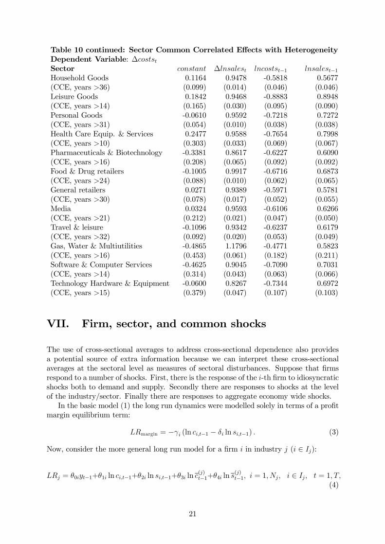
Table 10 continued: Sector Common Correlated E¤ects with HeterogeneityDependent Variable: �coststSector constant �lnsalest lncostst�1 lnsalest�1Household Goods 0.1164 0.9478 -0.5818 0.5677(CCE, years >36) (0.099) (0.014) (0.046) (0.046)Leisure Goods 0.1842 0.9468 -0.8883 0.8948(CCE, years >14) (0.165) (0.030) (0.095) (0.090)Personal Goods -0.0610 0.9592 -0.7218 0.7272(CCE, years >31) (0.054) (0.010) (0.038) (0.038)Health Care Equip. & Services 0.2477 0.9588 -0.7654 0.7998(CCE, years >10) (0.303) (0.033) (0.069) (0.067)Pharmaceuticals & Biotechnology -0.3381 0.8617 -0.6227 0.6090(CCE, years >16) (0.208) (0.065) (0.092) (0.092)Food & Drug retailers -0.1005 0.9917 -0.6716 0.6873(CCE, years >24) (0.088) (0.010) (0.062) (0.065)General retailers 0.0271 0.9389 -0.5971 0.5781(CCE, years >30) (0.078) (0.017) (0.052) (0.055)Media 0.0324 0.9593 -0.6106 0.6266(CCE, years >21) (0.212) (0.021) (0.047) (0.050)Travel & leisure -0.1096 0.9342 -0.6237 0.6179(CCE, years >32) (0.092) (0.020) (0.053) (0.049)Gas, Water & Multiutilities -0.4865 1.1796 -0.4771 0.5823(CCE, years >16) (0.453) (0.061) (0.182) (0.211)Software & Computer Services -0.4625 0.9045 -0.7090 0.7031(CCE, years >14) (0.314) (0.043) (0.063) (0.066)Technology Hardware & Equipment -0.0600 0.8267 -0.7344 0.6972(CCE, years >15) (0.379) (0.047) (0.107) (0.103)

VII. Firm, sector, and common shocks

The use of cross-sectional averages to address cross-sectional dependence also providesa potential source of extra information because we can interpret these cross-sectionalaverages at the sectoral level as measures of sectoral disturbances. Suppose that �rmsrespond to a number of shocks. First, there is the response of the i-th �rm to idiosyncraticshocks both to demand and supply. Secondly there are responses to shocks at the levelof the industry/sector. Finally there are responses to aggregate economy wide shocks.In the basic model (1) the long run dynamics were modelled solely in terms of a pro�t

margin equilibrium term:

LRmargin = � i (ln ci;t�1 � �i ln si;t�1) : (3)

Now, consider the more general long run model for a �rm i in industry j (i 2 Ij):

LRj = �0iyt�1+�1i ln ci;t�1+�2i ln si;t�1+�3i ln c(j)t�1+�4i ln s

(j)t�1; i = 1; Nj; i 2 Ij; t = 1; T;

(4)

21

where the superscript (j) in c(j)t�1 and s(j)t�1 indicate that these are averages of the industry

j in which the i-th �rm resides, and yt�1 is a (stationary) measure of the aggregateeconomy wide shock in the previous year.Including the cross-section averages, there are now 4 I(1) variables with temporal

variation, ln ci;t�1, ln si;t�1, ln c(j)t�1 and ln s

(j)t�1. All four have time series variation, while

only two, ln ci;t�1 and ln si;t�1, have cross-sectional variation as well. There are up to3 cointegrating relations between these variables, described below. This enriches ourspeci�cation of the long run equilibria and of the partial adjustment to these di¤erentequilibria. We use the latent factor structure to include these potential long run equilib-rium relationships in the model.

Pro�t margin equilibrium. The leading equilibrium relation, as before, is the pro�tmargin cointegration between log costs and log sales:

LRmargin = � i (ln ci;t�1 � �i ln si;t�1) : (5)

At the �rm level, costs adjust to their long run equilibrium with sales, with i as the rateof partial adjustment to the departure from equilibrium in the previous year, ln ci;t�1 ��i ln si;t�1. Potentially the long run coe¢ cient �i is heterogenous across �rms, but asdiscussed earlier is expected to have approximately unit value, �i � 1. For �rms withinthe same sector, the long run coe¢ cient may be homogeneous. Further, if �i = 1 forall �rms within the sector, the average pro�t margin is approximately �E (�i) =E ( i),where these two parameters (�xed e¤ect and partial adjustment) are allowed to varyacross �rms within a sector.

Market share equilibrium. The second equilibrium is a market share relation for sales,where sales of each �rm potentially maintain an equilibrium market share to total sales ofall �rms in a sector.There are only 2 long run coe¢ cients connecting the sales and averagesales terms in (4), and each equilibrium relation requires identi�cation of 2 parameters(the partial adjustment and long run coe¢ cient). Now, since the coe¢ cient on salesis �xed by the pro�t margin equilibrium (5), these 2 long run coe¢ cients cannot beseparately identi�ed.However, two observations can be made. First, there is potentially a restriction that

would ensure identi�cation. As discussed above, the long run e¤ect of sales on costsis likely to be close to unity (�i � 1), even if the short run dynamic e¤ect suggestsoperating leverage (�i < 1). In fact, our empirical results show that this relation holdsapproximately across all the sectors. Hence imposing this constraint would allow usto identify the two long run coe¢ cients in the market share equilibrium. Nevertheless,this is not satisfactory because it restricts the partial adjustment to both the above twoequilibria to be identical.Second, there is also a third relation implied by our model. Since costs and sales

are linked together in equilibrium through (5), sales being related to total sales througha hypothesized market share equilibrium suggests that costs of a �rm are also similarlyrelated to total costs of all �rms in the sector. Further, the partial adjustment and longrun e¤ect for both these equilibria should be exactly the same. Thus we have 4 long runcoe¢ cients (�rm sales, �rm costs, total sales and total costs) and 2 long run coe¢ cientsto be identi�ed. The above two constraints ensure that the two parameters of the market

22

share equilibrium are exactly identi�ed:

LRshare = � �i�ln ci;t�1 � ��i ln c

(j)t�1

�� �i

�ln si;t�1 � ��i ln s

(j)t�1

�= � �i

h(ln ci;t�1 + ln si;t�1)� ��i

�ln c

(j)t�1 + ln s

(j)t�1

�i: (6)

We call this cointegrating relationship the market share equilibrium.The pro�t market equilibrium and the market share equilibrium involve only two

variables, hence the partial adjustment term and long run slope have to be identi�ed,and two other lagged I(1) variables included with heterogenous slopes in the short rundynamic part of the model. The long run relations for these two equilibria are as follows:

LRj = � (��0i) yt�1 � (��1i)�ln ci;t�1 �

���2i�1i

�ln si;t�1

�(7)

+�3i ln c(j)t�1 + �4i ln s

(j)t�1

= � (��0i) yt�1 � (��2i)�(ln ci;t�1 + ln si;t�1)�

���4i�2i

��ln c

(j)t�1 + ln s

(j)t�1

��+(�1i � �2i) ln ci;t�1 + (�3i � �4i) ln c(j)t�1 (8)

Under the margin equilibrium, the model is estimated using the mean group estimator,setting the long run as (7) and including (9) in the short run dynamics. Assuminghomogeneity in the long run coe¢ cient �i = ��2i=�1i = �, the model is also estimated asa pooled mean group model. We apply a Hausman test for the homogeneity assumption.Estimation under the market share equilibrium is similar, in this case using (8) as thelong run speci�cation; however, in this case, pooled mean group estimation is not usedbecause equilibrium market shares for di¤erent �rms are expected to vary across �rms.

Cycle equilibrium The third equilibrium is the potential partial adjustment of logcosts and log sales (and therefore pro�t margin) to the economic cycle represented byLRcycle = � ��i yt�1. This equilibrium captures the e¤ect of an aggregate economy wideshock. Even though this equilibrium relation does not exploit cross section variation,it is important to allow for its potential in�uence in some sectors. Identi�cation of thecycle equilibrium is straightforward, as it involves a distinct variable yt�1 and only oneparameter has to be identi�ed from its coe¢ cient: the partial adjustment � ��i .In addition, the model includes short run dynamics. The short-run �rm-speci�c slope

coe¢ cient �i captures the e¤ect of an unanticipated shock to sales, which as discussedearlier, is our estimate of operating leverage. If a �rm can pass any shock to salesproportionately through to costs, �i = 1, otherwise if pass-through is incomplete, �i < 1.Allowing for slope heterogeneity across �rms, for each speci�c sector Ij, we testH0 : bj = 1against the left-tailed alternative H1 : bj < 1, where bj = E (�iji 2 Ij). If there isoperating leverage, that is, if the null hypothesis is rejected, we investigate potentialreasons for incomplete pass-through.

VIII. Determinants of operating leverage

There are several reasons why pass-through may be incomplete. The costs of employ-ment or �xed capital may be sticky. Alternatively, the �rm may intend to make priceadjustments, rather than quantity adjustments, but �nds that prices are sticky on the

23

downside, leading to an asymmetric adjustment of costs to sales. To test these conjec-tures, we model the short run e¤ect, �i, as a function of employment (nit), the log of real�xed capital (kit), and an indicator that sales have positive growth over the previous year(I (� ln sit > 0)). Thus, for sector Ij:

�i = �0i + �1iI (� ln sit > 0) + �2ikit + �3init + �4ini;t+1; i 2 Ij: (9)

�1i now measures the short run e¤ect of asymmetry and �2i measures the e¤ect of stickycapital costs. Descriptive analysis of the data suggests that many �rms adjust labourwith a lag, so �3i and �4i now capture the sticky costs associated with labour adjustmentin terms of contemporaneous and one-year ahead labour costs.Combining (4) with (9) provides our estimation model. �0i captures residual operating

leverage e¤ects after controlling for these sources of operating leverage. We test residualoperating leverage as H0 : E (�0i) = 1 versus H1 : E (�0i) < 1. The asymmetry and stickycapital channels are tested as H0 : E (�1i) = 0 versus H1 : E (�1i) < 0, and H0 : E (�2i) =0 versus H1 : E (�2i) < 0 respectively, while the sticky labour explanation is tested asH0 : E (�3i) = E (�4i) = 0 against the alternative H1 : min fE (�3i) ; E (�4i)g < 0.Employment (nit) is measured by number of employees. We use a Hodrik Prescott

�lter of quarterly output per capita averaged over the four quarters of every calendaryear as a measure of the business cycle (yt).6 Capital (kit) is measured as logarithm ofgross �xed assets (in real terms), while sit and cit represent sales revenue and cost ofsales respectively, in real terms. The model is estimated separately for �rms in each of 25sectors.7 We draw inferences on average slopes across the cross-section using the meangroup estimator of the individual �rm estimates and corresponding standard errors. Ifthe long run e¤ect is homogeneous across the �rms (�i = �) more e¢ cient inferences aredelivered by pooled mean group estimation. This means that while the individual shortrun responses of shocks to sales are allowed to vary across �rms, the long run relationshipbetween costs and sales are tested, and accordingly constrained, to be equal.We estimate the full model using the pooled mean group (PMG) method and including

�rm �xed e¤ects, short run dynamics (9) and the long run margin speci�cation (7) asan unrestricted model. We also estimated restricted models omitting short run dynamicsand long run equilibria, retaining in each case the components of the base model (1). Thisprovides us with (pseudo) likelihood ratio tests for the joint signi�cance of our short runand long run speci�cations. Detailed results are not reported, but all sectors reject thenull hypothesis that our speci�cation of short run dynamics and long run equilibria arenot signi�cant.8 We also estimate the full model as a mean group (MG), that is, withoutthe assumption that there is a homogeneous long run pro�t margin coe¢ cient for each�rm within the sector.

6Machin and van Reenen (1993) used unemployment rate as a measure of the business cycle. This

measure is based on the assumption of the unemployment rate is stationary, which is not true for the

long time period that our study covers.

7Using the Stata program xtpmg (Blackburne III and Frank, 2007).

8For the "Healthcare Equipment & Services" sector, pooled mean group estimation omitting short

run dynamics does not converge. This is likely due to an extremely �at nature of the pseudo log-likelihood

surface. This we take as evidence of a rejection of the null hypothesis of no short run dynamics, beyond

�i� ln sit included our base model.

24

A Hausman test (Wu, 1973; Hausman, 1978) is conducted to verify the validity ofthe common long run e¤ect assumption underlying the PMG estimates. In 23 of the 25sectors (except Industrial Metals and General Retailers), the null hypothesis of validityof the PMG assumption cannot be rejected at the 5% signi�cance level. These results arereported in Table 9 below.9 This provides con�rmation that a homogeneous costs-salesequilibrium relationship exists within most sectors.Nonetheless the e¢ ciency gain from making the PMG assumption is not always sub-

stantial. Because of considerable attrition in the data, the estimation can only be con-ducted over a limited sample of �rms that have a substantial number of years of data,which in turn leads to larger standard errors for the PMG estimates. This data issueis considerably reduced for mean group estimation. Hence, our choice between PMGand MG estimates is based on validity of the PMG assumption but also on sample sizeconsiderations. Table 9 reports the chosen model for each of the 25 sectors, the minimumnumber of years of data for sampled �rms within the sector, together with the numberof �rms and the number of �rm-year observations in each case.We also estimate a model using the market share speci�cation of the long run equilib-

rium (8) using the mean group method only; this provides us with estimates of a partialadjustment to the market share equilibrium. The pooled mean group assumption of acommon long run coe¢ cient is expected to be invalid in this case, since all �rms withina sector are not expected to have the same market share in equilibrium, and hence PMGestimation is not conducted. Estimates of partial adjustment to the third (business) cycleequilibrium are also obtained. Both the PMG and MG models provide evidence of thisequilibrium relationship only for a few sectors, indicating thereby that sectoral cyclesare often asynchronous with the aggregate business cycle. In e¤ect, the pro�t marginequilibrium captures sector-speci�c cyclical activity in our context.

9In 3 other sectors �Beverages, Leisure Goods and Technology Hardware & Equipment �the null

hypothesis of homogenous long run pro�t margin coe¢ cient is rejected at the 10 percent level.

25

Table 9: Estimates of long run coefficient on log­sales and partial adjustment terms                                (coefficients on common correlated effects terms are not reported)

Log­sales Margin adj. Mkt.share adj. Cycle adj.Oil & Gas Producers 36 467 ­1.2705 1.0179 ­0.5949 ­0.4242 ­0.8378

(pooled mean group, years >8) (0.961) (0.007) (0.229) (0.112) (1.028)Chemicals 24 744 ­0.0388 1.0049 ­0.6401 ­0.6524 0.1197

(pooled mean group, years >27) (0.112) (0.003) (0.128) (0.078) (0.126)Forestry & Paper 16 307 ­0.1689 1.0880 ­0.4704 ­0.5906 0.0338

(mean group, years >17) (0.136) (0.086) (0.136) (0.114) (0.132)Industrial Metals 30 448 ­0.2626 0.7598 ­0.3485 ­0.3137 ­0.4187

(mean group, years >8) (0.443) (0.075) (0.195) (0.113) (0.208)Construction & Materials 33 1103 ­0.1465 0.9966 ­0.5386 0.0199 ­0.3703

(pooled mean group, years >31) (0.101) (0.004) (0.058) (0.423) (0.291)Aerospace & Defense 16 401 ­0.4300 1.0995 ­0.8604 ­0.6939 ­0.0418

(mean group, years >13) (0.319) (0.092) (0.222) (0.169) (0.296)General Industrials 19 565 ­0.1266 1.0116 ­0.5568 ­0.6452 ­0.1314

(pooled mean group, years >23) (0.056) (0.004) (0.083) (0.092) (0.127)Electronic & Electrical Equipment 40 1043 ­0.1369 0.9875 ­0.3974 ­0.6797 0.0132

(pooled mean group, years >21) (0.100) (0.005) (0.124) (0.077) (0.098)Industrial Engineering 43 1319 0.1197 0.9869 ­0.6021 ­0.5964 0.0681

(mean group, years >31) (0.109) (0.027) (0.045) (0.046) (0.155)Industrial Transportation 38 776 ­0.0256 1.0152 ­0.7396 ­0.7129 ­0.6395

(mean group, years >18) (0.098) (0.017) (0.137) (0.082) (0.399)Support Services 32 1123 ­0.1040 0.9912 ­0.3897 0.0262 0.0540

(pooled mean group, years >32) (0.076) (0.001) (0.067) (0.576) (0.041)Automobiles & Parts 9 267 0.1454 1.0205 ­0.5840 ­0.7257 0.1285

(pooled mean group, years >12) (0.154) (0.009) (0.142) (0.135) (0.097)Beverages 28 761 ­0.3719 0.5852 ­0.4736 ­0.4748 ­0.2509

(mean group, years >19) (0.325) (0.292) (0.087) (0.086) (0.056)Food Producers 40 941 ­0.0604 1.0050 ­0.6635 ­0.7408 0.0123

(pooled mean group, years >19) (0.082) (0.001) (0.075) (0.075) (0.090)Household Goods 7 263 ­0.1178 1.0230 ­0.3928 ­0.4071 0.1820

(pooled mean group, years >36) (0.121) (0.014) (0.058) (0.069) (0.224)Leisure Goods 10 198 0.1078 0.9930 ­0.6047 3.1371 0.2044

(pooled mean group, years >14) (0.119) (0.013) (0.101) (3.506) (0.195)Personal Goods 18 559 0.1988 1.0136 ­0.6402 ­0.6484 ­0.2680

(pooled mean group, years >31) (0.148) (0.004) (0.105) (0.064) (0.271)Health Care Equip. & Services 19 431 ­0.2617 1.0408 ­0.5839 ­0.7988 ­0.1305

(pooled mean group, years >17) (0.150) (0.006) (0.136) (0.131) (0.295)Pharmaceuticals & Biotechnology 21 361 0.3116 1.0122 ­0.4821 ­0.3160 1.1543

(mean group, years >11) (0.654) (0.323) (0.151) (0.111) (1.189)Food & Drug Retailers 10 288 0.1426 0.8878 ­0.6334 ­0.6301 ­0.1115

(mean group, years >24) (0.062) (0.099) (0.140) (0.141) (0.069)General Retailers 29 898 ­0.2299 0.9055 ­0.6224 ­0.5529 ­0.0613

(mean group, years >30) (0.173) (0.056) (0.098) (0.061) (0.085)Media 41 1013 ­0.0708 1.0024 ­0.5686 ­0.6578 0.4366

(pooled mean group, years >21) (0.145) (0.002) (0.061) (0.066) (0.439)Gas, Water & Multiutilities 11 179 0.1253 0.7735 ­0.2564 ­1.6307 1.1015

(pooled mean group, years >15) (0.294) (0.000) (0.111) (0.886) (6.842)Software & Computer Services 30 583 ­0.1941 1.0249 ­0.7663 ­0.8704 1.4897

(pooled mean group, years >16) (0.186) (0.001) (0.127) (0.129) (0.794)Technology Hardware & Equipment 27 402 0.3267 0.1684 ­0.8777 ­0.6939 11.4419

(mean group, years >8) (0.629) (0.535) (0.227) (0.204) (11.162)

estimates (p ­values in parentheses)Bold (Italics ): Significant at 5% (10%)

Long­run ­ Margin, Mkt. share & Cycle eqbm.Sector No. offirms

Firm­years

Constant

Finally, we estimate two restricted models. First, we exclude the latent factor struc-ture (common correlated e¤ects and lagged business cycle). Second, we use only thebase model (1). A comparison of estimates of the coe¢ cient on sales growth from theshort run dynamics for the full model, with those from the restricted models, allows someinferences about the operating leverage hypothesis.

26

Speci�cally, we examine:

(a) how large the operating leverage e¤ect would appear to be if we considered partialadjustment only to the pro�t margin equilibrium and we ignored spatial strongdependence;

(b) how much is explained by the two other potential equilibria and correspondinglatent factors; and

(c) how much is explained by sticky labour costs, sticky capital and asymmetric priceadjustments.

Finally, we conduct cross section dependence (CD) tests (Pesaran, 2013) on the resid-uals of our model to ensure that our speci�cation of latent factors and equilibria hasmitigated issues relating to strong dependence; these tests are not reported, but areavailable on request.

A. Long run equilibria

Table 9 reports estimates of the long run coe¢ cient on lagged (log) sales (pro�t marginequilibrium) together with partial adjustment to the three potential equilibrium relation-ships investigated here. There is substantial evidence of cointegration, supporting theexistence of a long run pro�t margin equilibrium relationship between log costs and logsales. The partial adjustment to this equilibrium shows substantial variation across thesectors, and is statistically signi�cant at the 5% level in 24 out of 25 sectors, and the 10%level in the remaining sector, Industrial Metals. Correspondingly, the long run e¤ect ofsales on costs is numerically close to �i = 1 in 21 sectors out of 25. Partial adjustment tothis equilibrium is slow in Industrial Metals and Gas, and Water & Multiutilities (�0:35and �0:26 respectively). In Technology Hardware & Equipment there is strong partialadjustment (�0:88), but e¤ectively to a �xed cost equilibrium.There is evidence (signi�cant at the 5% level) of a long run market share equilibrium

in 21 out of 25 sectors. By contrast, the data suggest that in Construction & Materials,Support Services, and Leisure Goods, perhaps because competition is so severe thatmarket shares of �rms are continuously updated and do not �uctuate around �rm speci�cequilibrium levels.There is little evidence of a partial adjustment to the economic cycle equilibrium,

which was the central focus of investigation in Machin and van Reenen (1993). OnlyIndustrial Metals and Beverages show signi�cant (at the 5% level) evidence of partial ad-justment to the business cycle, and Industrial Transportation and Food & Drug Retailersshow weak evidence signi�cant at the 10% level.There are two ways to interpret these results. From an econometric point of view,

latent factors account for most of the strong dependence in the data, and are in turnmodeled using common correlated e¤ects. Hence, a measured factor such as the businesscycle may consequently show considerably less importance. From an industrial economicspoint of view, sectoral cycles in the UK are often claimed to be largely asynchronous sothat an aggregate economic cycle may not appropriately capture cyclical patterns at theindustry level. The results are consistent with this inetrpretation.

27

Table 10: Estimates of short run effects of sales growth and operating leverage explanations             (also growth coefficients in restricted models, excl. leverage explanations, and excl. factor structure as well)

Growth x Positive x Capital x Employment x Empl. (t+1)Oil & Gas Producers 0.6355 0.5603 ­0.0846 ­0.2654 0.0170 0.8219 0.9796

(pooled mean group, years >8) (0.184) (0.339) (0.282) (0.130) (0.146) (0.062) (0.038)Chemicals 0.9241 0.0255 0.0250 ­0.1420 ­0.2331 0.9849 0.9909

(pooled mean group, years >27) (0.067) (0.071) (0.109) (0.145) (0.107) (0.014) (0.011)Forestry & Paper 1.0690 ­0.1224 0.2753 0.7965 0.5244 0.9310 1.0066

(mean group, years >17) (0.082) (0.085) (0.116) (0.389) (0.321) (0.032) (0.066)Industrial Metals 0.9045 0.1056 0.3774 ­0.6460 0.3082 0.9153 0.9264

(mean group, years >8) (0.087) (0.097) (0.242) (0.503) (0.114) (0.017) (0.021)Construction & Materials 0.9806 0.0069 0.0564 ­0.1067 0.1262 0.9679 0.9710

(pooled mean group, years >31) (0.025) (0.028) (0.068) (0.078) (0.091) (0.011) (0.011)Aerospace & Defense 1.0238 ­0.0811 0.6017 0.5638 ­0.2567 0.9799 0.9850

(mean group, years >13) (0.130) (0.179) (0.592) (0.613) (0.185) (0.023) (0.022)General Industrials 0.9776 ­0.0256 ­0.1655 0.2958 0.0454 0.9684 0.9619

(pooled mean group, years >23) (0.056) (0.095) (0.120) (0.203) (0.098) (0.015) (0.017)Electronic & Electrical Equipment 1.0312 ­0.1179 0.1503 0.5427 0.9565 0.9525

(pooled mean group, years >21) (0.038) (0.055) (0.113) (0.339) (0.024) (0.023)Industrial Engineering 0.8631 0.1628 ­0.0507 ­0.1590 0.0763 0.9548 0.9566

(mean group, years >31) (0.058) (0.120) (0.094) (0.120) (0.049) (0.019) (0.021)Industrial Transportation 0.8486 0.0816 ­0.2735 0.1775 0.0503 0.9751 0.9119

(mean group, years >18) (0.123) (0.189) (0.179) (0.535) (0.151) (0.050) (0.100)Support Services 0.9833 ­0.0407 0.0645 0.0498 0.9789 0.9849

(pooled mean group, years >32) (0.021) (0.037) (0.046) (0.075) (0.012) (0.012)Automobiles & Parts 1.0420 ­0.1217 0.0983 0.3710 ­0.0199 0.9236 0.9314

(pooled mean group, years >12) (0.060) (0.076) (0.181) (0.104) (0.083) (0.035) (0.041)Beverages 1.0172 ­0.0479 ­0.0504 0.3554 ­0.0064 1.0748 1.0704

(mean group, years >19) (0.057) (0.067) (0.088) (0.351) (0.086) (0.080) (0.012)Food Producers 1.0891 ­0.1142 ­0.0057 0.1310 0.1526 0.9967 0.9966

(pooled mean group, years >19) (0.065) (0.069) (0.071) (0.094) (0.087) (0.008) (0.013)Household Goods 0.9350 0.0470 0.1551 ­0.2325 ­0.0049 0.9182 0.9176

(pooled mean group, years >36) (0.076) (0.080) (0.052) (0.068) (0.039) (0.039) (0.036)Leisure Goods 0.8625 0.1001 ­0.1077 ­0.0772 0.0634 0.8867 0.8972

(pooled mean group, years >14) (0.061) (0.060) (0.249) (0.131) (0.068) (0.029) (0.041)Personal Goods 0.9057 0.0595 0.0255 ­0.1587 0.0965 0.9709 0.9651

(pooled mean group, years >31) (0.035) (0.058) (0.073) (0.169) (0.075) (0.014) (0.015)Health Care Equip. & Services 1.1980 ­0.3581 0.0332 0.1800 ­0.1185 0.7644 0.7735

(pooled mean group, years >17) (0.246) (0.279) (0.231) (0.263) (0.261) (0.053) (0.072)Pharmaceuticals & Biotechnology 0.3700 0.1916 1.3560 ­3.6183 0.3018 0.8450 0.9367

(mean group, years >11) (0.539) (0.467) (1.179) (3.563) (0.164) (0.069) (0.063)Food & Drug Retailers ­6.4881 7.3715 0.0012 0.0194 ­0.0919 0.9844 0.9770

(mean group, years >24) (7.422) (7.422) (0.140) (0.077) (0.073) (0.020) (0.020)General Retailers 0.9233 0.1013 0.0213 0.0713 0.0291 1.0523 0.9795

(mean group, years >30) (0.045) (0.112) (0.070) (0.050) (0.115) (0.110) (0.010)Media 0.9466 0.0657 0.0161 ­0.0105 ­0.1377 0.9552 0.9467

(pooled mean group, years >21) (0.074) (0.095) (0.132) (0.196) (0.117) (0.017) (0.019)Gas, Water & Multiutilities 1.0622 0.5196 ­2.4321 0.1621 0.4086 1.0172 1.0917

(pooled mean group, years >15) (0.430) (0.730) (2.899) (0.918) (0.568) (0.069) (0.118)Software & Computer Services 1.1066 ­0.3539 0.0830 0.4925 0.5283 0.8566 0.8588

(pooled mean group, years >16) (0.213) (0.339) (0.184) (0.427) (0.331) (0.040) (0.051)Technology Hardware & Equipment 0.6380 ­0.3000 0.4666 ­0.9848 3.3236 0.7797 0.8207

(mean group, years >8) (0.121) (0.400) (0.328) (0.532) (3.378) (0.062) (0.064)

estimates (p ­values in parentheses)Bold (Italics ): Significant at 5% (10%)

LR + Onlygrowth

Sector Short­run ­ Sales growth & operating lev. Explanations Growth plusfactors

B. Short run dynamics

The principal subject of study in this paper is operating leverage, that is, the questionof whether, and by how much, the coe¢ cient on sales growth in short run dynamics fallsbelow unity, and to what extent this can be explained by asymmetric price adjustments,and by sticky labour and capital costs. Table 10 reports the estimates of the shortrun dynamics. In the full model the estimated short run coe¢ cient on sales growthis below unity in 16 of the 25 sectors, but this is statistically signi�cantly in only 5

28

sectors: Personal Goods, Industrial Engineering, Leisure Goods, Oil & Gas Producers,and General Retailers.However, estimates of the base model without latent factors and explanatory interac-

tion variables reveal a strikingly di¤erent story. The coe¢ cient is less that unity in allbut three sectors �Beverages, General Retailers and Gas, Water & Multiutilities �andsigni�cantly so in 17 sectors.A partial explanation comes from the use of long run latent factors and partial ad-

justment to di¤erent equilibria. When these common correlated e¤ects and the economiccycle are adjusted for, the coe¢ cient is lower than unity for 22 of the 25 sectors andthis is statistically signi�cant in 14. Mostly, this explanation comes from sticky employ-ment, but also in some sectors from �xed capital costs and asymmetric price adjustments.The combined e¤ect of asymmetric price adjustment and sticky labour and �xed capitalexplains operating leverage fully in 9 of these 14 sectors,10 including some of the most im-portant sectors in the UK economy. However, these inferences are more clearly apparentin statistical tests.Table 11 presents left-tailed tests of statistical hypotheses for operating leverage.

Based on estimates of the base model (1), there is a statistically signi�cantly (at 5%signi�cance level) evidence of margin contraction due to an unexpected shock to sales,in 17 out of 25 sectors. However, in the base model there is partial adjustment onlyto one cointegrating relationship, the log cost and log sales pro�t margin equilibrium.This model is probably too simplistic. We �nd evidence that in certain sectors costs andsales may also adjust to market share and economic cycle equilibria. Presumably, �rmswould anticipate partial adjustment to multiple equilibria in these sectors so that theunanticipated component in sales growth may be lower, and therefore also the operatingleverage channel.This turns out to be the case in most (11 out of 17) of the sectors where margin

shrink is signi�cantly lower after accounting for the other equilibrium relationships.11

Nevertheless, the operating leverage e¤ect is still statistically signi�cant in 14 sectors.In all but 5 of the sectors (Oil & Gas Producers, Industrial Engineering, Leisure Goods,Personal Goods and General Retailers) explanatory interaction variables fully explainoperating leverage up to the point where it is no longer statistically signi�cant. In themain, the explanation comes from sticky labour costs. This consistent with a world wherefrictions in the labour market ensure that, faced with an unanticipated fall in sales, �rmschoose not to, or may not be able to, fully adjust their employment.Our descriptive analysis suggests that employment is partly adjusted in the following

year and we allow for delayed adjustment in the estimated model. The sticky labourcosts explanation is statistically signi�cant in 9 sectors.12 In addition, sticky �xed capitalis also signi�cant, at the 10% level, in 2 other sectors, General Industrials and Industrial

10Industrial Metals, Construction & Materials, General Industrials, Electronic & Electrical Equip-

ment, Automobiles & Parts, Household Goods, Media, Software & Computer Services and Technology

Hardware & Equipment.

11Oil & Gas Producers, Forestry & Paper, Industrial Metals, Construction & Materials, Industrial

Engineering, Support Services, Automobiles & Parts, Leisure Goods, Healthcare Equipment & Services,

Software & Computer Services and Technology Hardware & Equipment.

12At the 5 percent level in 4 sectors - Oil & Gas Producers, Chemicals, Household Goods and Tech-

29

Transportation. So, in total, there are 11 sectors where sticky costs explain operatingleverage e¤ects.

Table 11: (Left­tailed) tests for operating leverage and its explanations

Only growth Incl. factors All variables Sticky capital Sticky employment AsymmetryOil & Gas Producers 2.8746 0.5326 1.9795 0.3001 2.0407 ­1.6551

(pooled mean group, years >8) (0.002) (0.297) (0.024) (0.382) (0.021) (0.951)Chemicals 1.1206 0.7980 1.1408 ­0.2286 2.1844 ­0.3608

(pooled mean group, years >27) (0.131) (0.212) (0.127) (0.590) (0.014) (0.641)Forestry & Paper 2.1661 ­0.1007 ­0.8400 ­2.3820 ­1.6321 1.4367

(mean group, years >17) (0.015) (0.540) (0.800) (0.991) (0.949) (0.075)Industrial Metals 5.0398 3.4266 1.1035 ­1.5620 1.2852 ­1.0937

(mean group, years >8) (0.000) (0.000) (0.135) (0.941) (0.099) (0.863)Construction & Materials 3.0201 2.7282 0.7777 ­0.8329 1.3709 ­0.2493

(pooled mean group, years >31) (0.001) (0.003) (0.218) (0.798) (0.085) (0.598)Aerospace & Defense 0.8930 0.6780 ­0.1836 ­1.0161 1.3860 0.4525

(mean group, years >13) (0.186) (0.249) (0.573) (0.845) (0.083) (0.325)General Industrials 2.0559 2.2674 0.3983 1.3792 ­0.4638 0.2711

(pooled mean group, years >23) (0.020) (0.012) (0.345) (0.084) (0.679) (0.393)Electronic & Electrical Equipment 1.7953 2.0648 ­0.8240 ­1.3290 ­1.6024 2.1355

(pooled mean group, years >21) (0.036) (0.019) (0.795) (0.908) (0.945) (0.016)Industrial Engineering 2.4420 2.0823 2.3670 0.5399 1.3268 ­1.3538

(mean group, years >31) (0.007) (0.019) (0.009) (0.295) (0.092) (0.912)Industrial Transportation 0.4974 0.8768 1.2272 1.5247 ­0.3317 ­0.4323

(mean group, years >18) (0.309) (0.190) (0.110) (0.064) (0.630) (0.667)Support Services 1.7187 1.2813 0.8089 ­1.4091 ­0.6609 1.1136

(pooled mean group, years >32) (0.043) (0.100) (0.209) (0.921) (0.746) (0.133)Automobiles & Parts 2.1555 1.6888 ­0.7046 ­0.5414 0.2396 1.5905

(pooled mean group, years >12) (0.016) (0.046) (0.759) (0.706) (0.405) (0.056)Beverages ­0.9389 ­5.6549 ­0.3037 0.5754 0.0742 0.7198

(mean group, years >19) (0.826) (1.000) (0.619) (0.283) (0.470) (0.236)Food Producers 0.3920 0.2671 ­1.3616 0.0805 ­1.3987 1.6456

(pooled mean group, years >19) (0.348) (0.395) (0.913) (0.468) (0.919) (0.050)Household Goods 2.1052 2.2594 0.8547 ­2.9752 3.4075 ­0.5887

(pooled mean group, years >36) (0.018) (0.012) (0.196) (0.999) (0.000) (0.722)Leisure Goods 3.9306 2.5350 2.2569 0.4333 0.5886 ­1.6766

(pooled mean group, years >14) (0.000) (0.006) (0.012) (0.332) (0.278) (0.953)Personal Goods 2.1377 2.3450 2.6856 ­0.3510 0.9370 ­1.0258

(pooled mean group, years >31) (0.016) (0.010) (0.004) (0.637) (0.174) (0.848)Health Care Equip. & Services 4.4063 3.1286 ­0.8038 ­0.1436 0.4538 1.2836

(pooled mean group, years >17) (0.000) (0.001) (0.789) (0.557) (0.325) (0.100)Pharmaceuticals & Biotechnology 2.2522 1.0052 1.1687 ­1.1496 1.0155 ­0.4104

(mean group, years >11) (0.012) (0.157) (0.121) (0.875) (0.155) (0.659)Food & Drug Retailers 0.7760 1.1305 1.0089 ­0.0083 1.2653 ­0.9931

(mean group, years >24) (0.219) (0.129) (0.157) (0.503) (0.100) (0.840)General Retailers ­0.4775 2.0691 1.7206 ­0.3044 ­0.2533 ­0.9059

(mean group, years >30) (0.683) (0.019) (0.043) (0.620) (0.600) (0.818)Media 2.6113 2.8486 0.7200 ­0.1220 1.1753 ­0.6951

(pooled mean group, years >21) (0.005) (0.002) (0.236) (0.549) (0.120) (0.756)Gas, Water & Multiutilities ­0.2499 ­0.7785 ­0.1447 0.8390 ­0.1766 ­0.7119

(pooled mean group, years >15) (0.599) (0.782) (0.558) (0.201) (0.570) (0.762)Software & Computer Services 3.5994 2.7469 ­0.4998 ­0.4510 ­1.1529 1.0444

(pooled mean group, years >16) (0.000) (0.003) (0.691) (0.674) (0.876) (0.148)Technology Hardware & Equipment 3.5544 2.8164 2.9876 ­1.4209 1.8518 0.7503

(mean group, years >8) (0.000) (0.002) (0.001) (0.922) (0.032) (0.227)

z ­stats (p ­values in parentheses)Bold (Italics ): Significant at 5% (10%)

Explanations for operating leverageTest for operating leverage (lower margin)Sector

There are 4 other sectors where asymmetric price adjustments provide an explanation;the e¤ect is statistically signi�cant at the 5% level in 2 sectors (Electronic & ElectricalEquipment and Food Producers) and at the 10% level in 2 others (Forestry & Paper

nology Hardware & Equipment, and at 10 percent in 5 other sectors - Industrial Metals, Construction

& Materials, Aerospace & Defence, Industrial Engineering and Food & Drug Retailers.

30

and Automobiles & Parts). We conjecture that the forces of domestic and internationalcompetition restrict producers in these sectors from being able to adjust prices fully onthe downside.

IX. Conclusions

In this paper we have sought to operationalise the analysis of operating leverage in amodel in which we allow for short run variations in margin but test and control for anequilibrating relationship for margins in the long run. To do this we use some recentdevelopments in panel econometrics which allows for heterogeneity in slopes and thepossibility of common factors. We found that aggregate models using data for all sectorsfailed to make full allowance for cross sectional dependence, and failed to adequatelycapture sectoral variation in operating leverage and its explanations. We examine howoperating leverage functions in 25 UK sectors. Our results suggest that the behaviour ofoperating leverage over the business cycle re�ects sticky labour costs and some degree ofasymmetric price adjustment. But we also �nd that there are two main equibrating longrun relationships to which operating pro�t adjusts �the relationship between costs andsales and a market share relationship between �rm sales and total sales in a sector.

References

[1] Acharya, V.; H. Almeida; and M. Campello. �Aggregate Risk and the Choice Be-tween Cash and Lines of Credit.�Journal of Finance, 68 (2013), 2059�2116.

[2] Bailey, N., Holly, S. and Pesaran, H.M. (2015) �A Two Stage Approach to Spatiotem-poral Analysis with Strong and Weak Cross-Sectional Dependence", Forthcoming,Journal of Applied Econometrics.

[3] Bhattacharjee, A., Higson, C., Holly, S.and Kattuman, P. (2009) \Business Failurein UK and US Quoted Firms: Impact of Macro-Economic Instability and the Roleof Legal Systems�. Review of Law and Economics.

[4] Bhattacharjee, A., Higson, C., Holly, S. and Kattuman, P. (2009) �Macro EconomicInstability and Business Exit: Determinants of Failures and Acquisitions of LargeUK Firms�. Economica, 76, 301, 108-131.

[5] Bhattacharjee, A. and Holly, S. (2013) �Understanding interactions in social net-works and committees�, Spatial Economic Analysis. 8, 1, 23-53.

[6] Blackburne, E.F. and Frank, M.W.. (2007). �Estimation of nonstationary heteroge-neous panels�, Stata Journal, StataCorp LP, 7, 2, 197-208.

[7] Bils, M., 1987. �The Cyclical Behavior of Marginal Cost and Price�, American Eco-nomic Review. 77, 5, 838-55.

[8] Bowman, R.G. (1979). �The Theoretical Relationship between the Systematic Riskand Financial (Accounting) Variables,�Journal of Finance 34, 617-630.

31

[9] Campello, M., and E. Giambona. �Real Assets and Capital Structure.�Journal ofFinancial and Quantitative Analysis, 48 (2013), 1333�1370.

[10] Carlson, M., A. Fisher, and R. Giammarino (2004). �Corporate Investment andAsset Price Dynamics: Implications for the Cross Section of Returns,� Journal ofFinance 59, 2577-2603.

[11] Chen, N. and F. Zhang (1998). �Risk and Return of Value Stocks,� Journal ofBusiness 71, 501-535.

[12] Cooper, I. (2006). �Asset pricing implications of non-convex adjustment costs andirreversibility of investment,�Journal of Finance , 61, pp. 139�170.

[13] Darrat, A. F. and Mukherjee, T. K. (2005) �Inter-Industry Di¤erences and the Im-pact of Operating and Financial Leverages on Equity Risk�, Review of FinancialEconomics.Spring 141-155.

[14] DeYoung, R. and K.P. Roland (2001). �Product Mix and Earnings Volatility atCommercial Banks: Evidence from a Degree of Total Leverage Model,�Journal ofFinancial Intermediation 10, 54-84.

[15] Dichev, I.D. (1998). �Is the Risk of Bankruptcy a Systematic Risk?� Journal ofFinance 53, 1131-1147.

[16] Dugan, Michael T., Donald Minyard, and Keith A. Shriver (1994) �A Re-examination of the Operating Leverage-Financial Leverage Tradeo¤�, Quarterly Re-view of Economics & Finance. Fall, 327-334.

[17] Fama, E.F. and K.R. French (1992). �The Cross-Section of Expected Stock Returns,�Journal of Finance 47, 427-465.

[18] Fama, E.F. and K.R. French (1996). �Multifactor Explanations of Asset PricingAnomalies,�Journal of Finance 51, 55-84.

[19] Farinas, J.C. and Huergo, E. (2003) "Pro�t Margins, Adjustment costs and theBusiness Cycle: An Application to Spanish Manufacturing Firms". Oxford Bulletinof Economics and Statistics, 65, 1, 49-72.

[20] Ferri, M.G. and W.H. Jones (1979). �Determinants of Financial Structure: A NewMethodological Approach,�Journal of Finance 34, 631-644.

[21] Gertler, M. and Gilchrist, S. (1994). �Monetary Policy, Business Cycles and theBehavior of Small Manufacturing Firms�, Quarterly Journal of Economics, 109, 2,309-340.

[22] Geroski, P.A. and P. Gregg (1997). UK company performance in adversity, Cam-bridge University Press, Cambridge.

[23] Gri¢ n, H.F. and M.T. Dugan (2003). �Systematic Risk and Revenue Volatility,�Journal of Financial Research, 26, 179-189.

[24] Gri¢ n, J.M. (2002). �Are the Fama and French factors global or country speci�c?�Review of Financial Studies 15(3), 783-803.

32

[25] Gourio, F. (2005). �Operating Leverage, Stock Market Cyclicity, and the Cross-Section of Returns,�working paper, Jan.

[26] Gourio, F. (2008) �Disasters and Recoveries,�American Economic Review, 98, num-ber 2,

[27] Gulen, H., Y. Xing, and L. Zhang. (2008). �Value versus Growth: Time-VaryingExpected Stock Returns,�University of Michigan Working Paper.

[28] Ghosh, Dilip K. and Robert G. Sherman (1993), �Leverage, Resource Allocation andGrowth�,Journal of Business Finance & Accounting. June, 575-582.

[29] Gottfries, Nils (1991). �Customer Markets, Credit Market Imperfections and RealPrice Rigidity�, Economica, 58, 231, 317-23, August.

[30] Green, E.J. and Porter, R.H. (1984) �Noncooperative collusion under imperfect pricecompetition�, Econometrica, 52, 87-100.

[31] Hamada, R.S. (1972). �The E¤ect of the Firms Capital Structure on the SystematicRisk of Common Stock,�Journal of Finance 27, 435-452.

[32] Hausman, J.A. (1978) �Speci�cation tests in econometrics�, Econometrica, 46, 125l-1271.

[33] Higson, C., Holly, S., Kattuman, P. and Platis, S. (2004) "The Business Cycle,Macroeconomic Shocks and the Cross Section: The Growth of UK Quoted Compa-nies", Economica, 71, 281, 299-318.

[34] Holly, S., Pesaran, H.M. and Yamagata, T. (2011) �The Spatial and Temporal Dif-fusion of House Prices in the UK�, Journal of Urban Economics , vol 69, pp. 2-23.

[35] Ho, Y.K., Z. Xu, and C.M. Yap, C.M. (2004). �R&D Investment and SystematicRisk,�Accounting and Finance 44, 393-418.

[36] Hu¤man, L., 1983, �Operating Leverage, Financial Leverage, and Equity Risk,�Journal of Banking and Finance, 7, 197-212.

[37] Im, K.S., Pesaran, M.H. and Shin, Y. (2003) �Testing for Unit Roots in heteroge-neous Panels�. Journal of Econometrics. 115:53-74

[38] James, C. and Kizilaslan, A. �Asset Speci�city, Industry-Driven Recovery Risk, andLoan Pricing�Journal of Financial and Quantitative Analysis Vol. 49, No. 3, June2014, pp. 599�631

[39] Kahl, M., Lunn, J. and Nilsson, M. (2013). �Operating leverage and corporate �-nancial policies�. Working Paper, University of Colorado at Boulder.

[40] Lang, Larry, Eli Ofek, and Rene M. Stulz (1996), �Leverage, Investment, and FirmGrowth�, Journal of Financial Economics January, 3-29.

[41] Li, Rong-Jen and Glenn V. Henderson, Jr. (1991) �Combined Leverage and StockRisk�, Quarterly Journal of Business & Finance. Winter. 18-39.

33

[42] Lev, B. (1974). �On the association between operating leverage and risk,�Journalof Financial and Quantitative Analysis. 9,4, 627�641.

[43] Ljungqvist, A. andW.J.Wilhelm, Jr. (2005). �Does Prospect Theory Explain IPOMarket Behavior?�Journal of Finance 60, 1759-1790.

[44] Lord, R., 1996, �The Impact of Operating and Financial Risk on Equity Risk,�Journal of Economics and Finance, 20, 27-38.

[45] Lord, R., 1998, �Properties of Time-Series Estimates of Degree of Leverage Mea-sures,�Financial Review 33, 69-84.

[46] Machin, S and Van Reenen, J. (1993) �Pro�t margins and the business cycle: ev-idence from UK manufacturing �rms�. Journal of Industrial Economics, XLI (1).29-50.

[47] Mandelker, G.N. and Rhee, S.G. (1984). �The Impact of the Degrees of Operatingand Financial Leverage on Systematic Risk of Common Stock,�Journal of Financialand Quantitative Analysis 19, 45-57.

[48] Mensah, Y.M., �Adjusted Accounting Beta, Operating Leverage and FinancialLeverage as Determinants of Market Beta: A Synthesis and Empirical Evaluation,�Review of Quantitative Finance and Accounting, 2, p187�203, 1992

[49] Novy-Marx, R.(2007a), �Real Options and Investment in a Dynamic Model ofOligopoly,�working paper.

[50] Novy-Marx, R. (2007b), �Investment-Cash Flow Sensitivity and the Value Premium�working paper.

[51] Novy-Marx, R. (2011) �Operating Leverage�, Review of Finance. 15, 1, 103-134.

[52] O�Brien, T.J. and Vanderheiden P.A. (1987). �Empirical Measurement of OperatingLeverage for Growing Firms�. Financial Management 16, 45-53.

[53] Petersen, M.A. (2009) �Estimating Standard Errors in Finance Panel Data Sets:Comparing Approaches�, Review of Financial Studies, 22, 1, 435-480.

[54] Pesaran, M. H. (2006). �Estimation and inference in large heterogenous panels withmultifactor error structure�. Econometrica 74, 967�1012.

[55] Pesaran, M.H. (2013). Testing weak cross-sectional dependence in large panels.Econometric Reviews, forthcoming.

[56] Pesaran, M. H. and R. Smith (1995). �Estimating long-run relationships from dy-namic heterogeneous panels�. Journal of Econometrics 68, 79�113.

[57] Pesaran, M. H., Shin, Y. and Smith, R. J. (2000). �Structural analysis of vector errorcorrection models with exogenous I(1) variables�, Journal of Econometrics, 97, 2,293-343.

[58] Reid, G. C., Bhaskar, V. & Machin, S. (1993) �Price and Quantity Adjustment overthe Business Cycle: Evidence from Survey Data�, Oxford Economic Papers. 45, 2,p. 257-68

34

[59] Rosett, J.G. (2001). �Equity Risk and the Labor Stock: The Case of Union Con-tracts,�Journal of Accounting Research 39, 337-364.

[60] Rotemberg, J.J. and Saloner, G. (1986) �A supergame-theoretic model of price warsduring booms�, American Economic Review, 76, 390-407.

[61] Rubinstein, M.E., 1973, �A Mean-Variance Synthesis of Corporate Financial The-ory,�Journal of Finance 28, 167-182.

[62] Shumway, T. and V. Warther, 1999, �The Delisting Bias in CRSP�s NASDAQ Dataand Its Implications for the Size E¤ect,�Journal of Finance 54, 2361-2379.

[63] Stock, J.H. (1987). �Asymptotic Properties of Least Squares Estimation of Cointe-grating Vectors,�Econometrica, 55, 1035-1056.

[64] Stock, J.H. and M.W. Watson (1993). �A Simple Estimator of Cointegrating Vectorsin Higher Order Integrated Systems,�Econometrica, 61, 783-820.

[65] Wu, D.-M. (1973) �Alternative tests of independence between stochastic regressorsand disturbances�, Econometrica, 41, 733-750.

[66] Zhang, L., 2005, �The Value Premium,�Journal of Finance 60, 67-103.

35