operating and financial leverage - جامعة نزوى · operating leverage operating leverage is...

••

419

16Operating and Financial Leverage

Contents

l Operating LeverageBreak-Even Analysis • Degree of OperatingLeverage (DOL) • DOL and the Break-EvenPoint • DOL and Business Risk

l Financial LeverageEBIT-EPS Break-Even, or Indifference, Analysis• Degree of Financial Leverage (DFL) • DFL andFinancial Risk

l Total LeverageDegree of Total Leverage (DTL) • DTL and TotalFirm Risk

l Cash-Flow Ability to Service DebtCoverage Ratios • Probability of Cash Insolvency

l Other Methods of AnalysisComparison of Capital Structure Ratios •Surveying Investment Analysts and Lenders •Security Ratings

l Combination of Methods

l Key Learning Points

l Questions

l Self-Correction Problems

l Problems

l Solutions to Self-Correction Problems

l Selected References

Objectives

After studying Chapter 16, you should be able to:

l Define operating and financial leverage andidentify causes of both.

l Calculate a firm’s operating break-even (quan-tity) point and break-even (sales) point.

l Define, calculate, and interpret a firm’s degree ofoperating, financial, and total leverage.

l Understand EBIT-EPS break-even, or indiffer-ence, analysis, and construct and interpret anEBIT-EPS chart.

l Define, discuss, and quantify “total firm risk”and its two components, “business risk” and“financial risk.”

l Understand what is involved in determining the appropriate amount of financial leverage for a firm.

FUNO_C16.qxd 9/19/08 17:19 Page 419

When a lever is used properly, a force applied at one point is transformed, or magnified, intoanother, larger force or motion at some other point. This comes most readily to mind whenconsidering mechanical leverage, such as that which occurs when using a crowbar. In a busi-ness context, however, leverage refers to the use of fixed costs in an attempt to increase (orlever up) profitability. In this chapter we explore the principles of both operating leverageand financial leverage. The former is due to fixed operating costs associated with the pro-duction of goods or services, whereas the latter is due to the existence of fixed financing costs – in particular, interest on debt. Both types of leverage affect the level and variability ofthe firm’s after-tax earnings, and hence the firm’s overall risk and return.

Operating LeverageOperating leverage is present any time a firm has fixed operating costs – regardless of volume.In the long run, of course, all costs are variable. Consequently, our analysis necessarilyinvolves the short run. We incur fixed operating costs in the hope that sales volume will produce revenues more than sufficient to cover all fixed and variable operating costs. One ofthe more dramatic examples of an effect of operating leverage is the airline industry, where alarge proportion of total operating costs is fixed. Beyond a certain break-even load factor, eachadditional passenger essentially represents straight operating profit (earnings before interestand taxes, or EBIT) to the airline.

It is essential to note that fixed operating costs do not vary as volume changes. These costs include such things as depreciation of buildings and equipment, insurance, part of theoverall utility bills, and part of the cost of management. On the other hand, variable operat-ing costs vary directly with the level of output. These costs include raw materials, direct laborcosts, part of the overall utility bills, direct selling commissions, and certain parts of generaland administrative expenses.

One interesting potential effect caused by the presence of fixed operating costs (operatingleverage) is that a change in the volume of sales results in a more than proportional change inoperating profit (or loss). Thus, like a lever used to magnify a force applied at one point intoa larger force at some other point, the presence of fixed operating costs causes a percentagechange in sales volume to produce a magnified percentage change in operating profit (or loss).(A note of caution: remember, leverage is a two-edged sword – just as a company’s profits canbe magnified, so too can the company’s losses.)

This magnification effect is illustrated in Table 16.1. In Frame A we find three differentfirms possessing various amounts of operating leverage. Firm F has a heavy amount of fixedoperating costs (FC) relative to variable costs (VC). Firm V has a greater dollar amount ofvariable operating costs than of fixed operating costs. Finally, Firm 2F has twice the amountof fixed operating costs as does Firm F. Notice that, of the three firms shown, Firm 2F has (1)the largest absolute dollar amount of fixed costs and (2) the largest relative amount of fixedcosts as measured by both the (FC/total costs) and (FC/sales) ratios.

Each firm is then subjected to an anticipated 50 percent increase in sales for next year.Which firm do you think will be more sensitive to the change in sales: that is, for a given percentage change in sales, which firm will show the largest percentage change in operatingprofit (EBIT)? (Most people would pick Firm 2F – because it has either the largest absolute orthe largest relative amount of fixed costs. Most people would be wrong.)

Part 6 The Cost of Capital, Capital Structure, and Dividend Policy

420

••

It does not do to leave a live dragon out of your calculations, if youlive near him.

—J. R. R. TOLKIENThe Hobbit

Leverage The use of fixed costs in anattempt to increase(or lever up)profitability.

Operating leverageThe use of fixedoperating costs by the firm.

Financial leverageThe use of fixedfinancing costs by the firm. The Britishexpression is gearing.

FUNO_C16.qxd 9/19/08 17:19 Page 420

The results are shown in Frame B of Table 16.1. For each firm, sales and variable costsincrease by 50 percent. Fixed costs do not change. All firms show the effects of operating lever-age (that is, changes in sales result in more than proportional changes in operating profits).But Firm F proves to be the most sensitive firm, with a 50 percent increase in sales leading toa 400 percent increase in operating profit. As we have just seen, it would be an error to assumethat the firm with the largest absolute or relative amount of fixed costs automatically showsthe most dramatic effects of operating leverage. Later, we will come up with an easy way todetermine which firm is most sensitive to the presence of operating leverage. But, before wecan do so, we need to learn how to study operating leverage by means of break-even analysis.

l l l Break-Even AnalysisTo illustrate break-even analysis as applied to the study of operating leverage, consider a firmthat produces a high-quality child’s bicycle helmet that sells for $50 a unit. The company hasannual fixed operating costs of $100,000, and variable operating costs are $25 a unit regard-less of the volume sold. We wish to study the relationship between total operating costs andtotal revenues. One means for doing so is with the break-even chart in Figure 16.1, whichshows the relationship among total revenues, total operating costs, and profits for various levels of production and sales. As we are concerned only with operating costs at this point, wedefine profits here to mean operating profits before taxes. This definition purposely excludesinterest on debt and preferred stock dividends. These costs are not part of the total fixed oper-ating costs of the firm and have no relevance when it comes to analyzing operating leverage.They are taken into account, however, when we analyze financial leverage in the next section.

Break-Even (Quantity) Point. The intersection of the total costs line with the total revenuesline determines the break-even point. The break-even point is the sales volume required fortotal revenues to equal total operating costs or for operating profit to equal zero. In Figure16.1 this break-even point is 4,000 units of output (or $200,000 in sales). Mathematically, wefind this point (in units) by first noting that operating profit (EBIT) equals total revenuesminus variable and fixed operating costs:

16 Operating and Financial Leverage

421

••

Break-even analysis Atechnique for studyingthe relationshipamong fixed costs,variable costs, salesvolume, and profits. It is also calledcost/volume/profit(C/V/P) analysis.

Break-even chart Agraphic representationof the relationshipbetween totalrevenues and totalcosts for variouslevels of productionand sales, indicatingareas of profit andloss.

Break-even pointThe sales volumerequired so that totalrevenues and totalcosts are equal; maybe expressed in unitsor in sales dollars.

Table 16.1Effect of operatingleverage showing thatchanges in salesresult in more thanproportional changesin operating profit(EBIT)

Frame A: Three firms before changes in sales

Firm F Firm V Firm 2FSales $10,000 $11,000 $19,500Operating costs

Fixed (FC) 7,000 2,000 14,000Variable (VC) 2,000 7,000 3,000

Operating profit (EBIT) $ 1,000 $ 2,000 $ 2,500Operating leverage ratios

FC/total costs 0.78 0.22 0.82FC/sales 0.70 0.18 0.72

Frame B: Three firms after 50 percent increases in sales in following year

Firm F Firm V Firm 2FSales $15,000 $16,500 $29,250Operating costs:

Fixed (FC) 7,000 2,000 14,000Variable (VC) 3,000 10,500 4,500

Operating profit (EBIT) $ 5,000 $ 4,000 $10,750

Percent change in EBIT(EBITt − EBITt −1)/EBITt −1 400% 100% 330%

FUNO_C16.qxd 9/19/08 17:19 Page 421

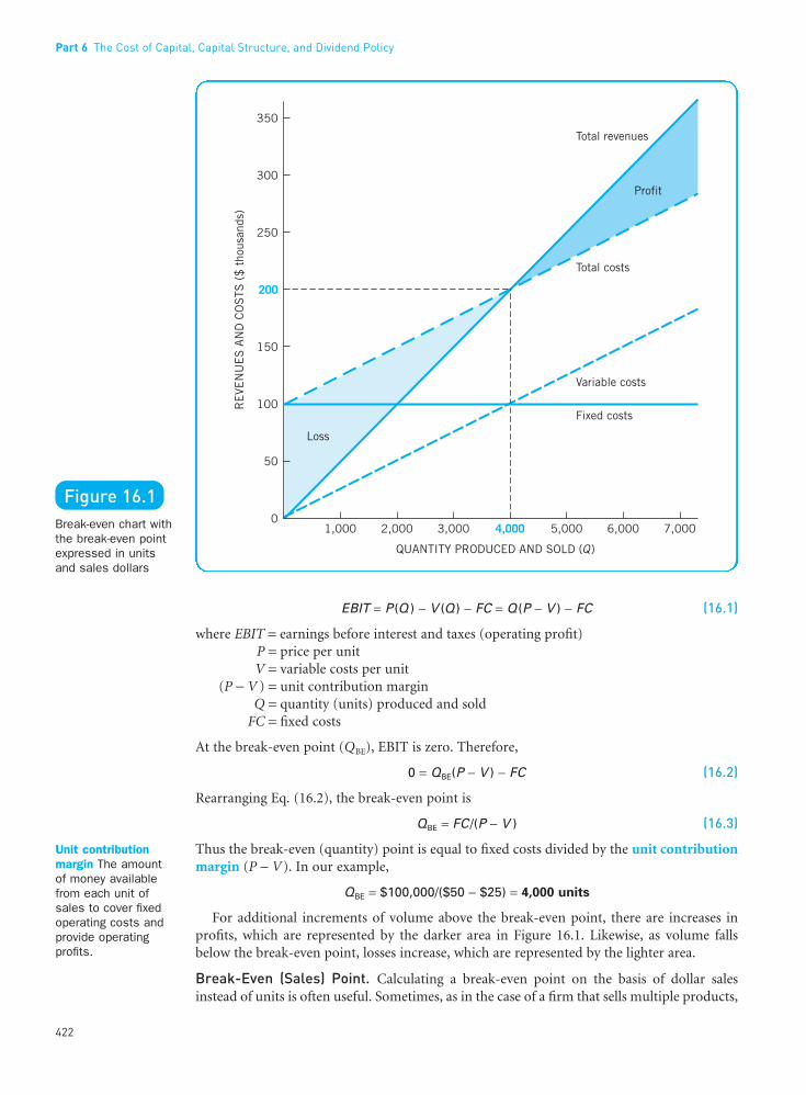
EBIT = P (Q ) − V (Q ) − FC = Q (P − V ) − FC (16.1)

where EBIT = earnings before interest and taxes (operating profit)P = price per unitV = variable costs per unit

(P − V ) = unit contribution marginQ = quantity (units) produced and sold

FC = fixed costs

At the break-even point (QBE), EBIT is zero. Therefore,

0 = QBE(P − V ) − FC (16.2)

Rearranging Eq. (16.2), the break-even point is

QBE = FC /(P − V ) (16.3)

Thus the break-even (quantity) point is equal to fixed costs divided by the unit contributionmargin (P − V). In our example,

QBE = $100,000/($50 − $25) = 4,000 units

For additional increments of volume above the break-even point, there are increases inprofits, which are represented by the darker area in Figure 16.1. Likewise, as volume fallsbelow the break-even point, losses increase, which are represented by the lighter area.

Break-Even (Sales) Point. Calculating a break-even point on the basis of dollar salesinstead of units is often useful. Sometimes, as in the case of a firm that sells multiple products,


422

••

Figure 16.1Break-even chart withthe break-even pointexpressed in unitsand sales dollars

Unit contributionmargin The amount of money availablefrom each unit ofsales to cover fixedoperating costs andprovide operatingprofits.

FUNO_C16.qxd 9/19/08 17:19 22

it is a necessity. It would be impossible, for example, to come up with a meaningful break-even point in total units for a firm such as General Electric, but a break-even point based onsales revenues could easily be imagined. When determining a general break-even point for amultiproduct firm, we assume that sales of each product are a constant proportion of thefirm’s total sales.

Recognizing that at the break-even (sales) point the firm is just able to cover its fixed andvariable operating costs, we turn to the following formula:

SBE = FC + VCBE (16.4)

where SBE = break-even sales revenuesFC = fixed costs

VCBE = total variable costs at the break-even point

Unfortunately, we are now faced with a single equation containing two unknowns – SBE andVCBE. Such an equation is insolvable. Luckily, there is a trick that we can use in order to turnEq. (16.4) into a single equation with a single unknown. First, we need to rewrite Eq. (16.4)as follows:

SBE = FC + (VCBE /SBE)SBE (16.5)

Because the relationship between total variable costs and sales is assumed constant in linearbreak-even analysis, we can replace the ratio (VCBE/SBE) with the ratio of total variable coststo sales (VC/S) for any level of sales. For example, we can use the total variable costs and salesfigures from the firm’s most recent income statement to produce a suitable (VC/S) ratio. Inshort, after replacing the ratio (VCBE /SBE) with the “generic” ratio (VC/S) in Eq. (16.5), we get

SBE = FC + (VC /S )SBE

SBE[1 − (VC /S )] = FCSBE = FC / [1 − (VC /S )] (16.6)

For our example bicycle-helmet manufacturing firm, the ratio of total variable costs to salesis 0.50 regardless of sales volume. Therefore, using Eq. (16.6) to solve for the break-even(sales) point, we get

SBE = $100,000/[1 − 0.50] = $200,000

At $50 a unit, this $200,000 break-even (sales) point is consistent with the 4,000 unit break-even (quantity) point determined earlier [i.e., (4,000)($50) = $200,000].

TIP•TIP

You can easily modify break-even (quantity) Eq. (16.3) and break-even (sales) point Eq. (16.6)to calculate the sales volume (in units or dollars) required to produce a “target” operatingincome (EBIT) figure. Simply add your target or minimum desired operating income figureto fixed costs (FC) in each equation. The resulting answers will be your target sales volume– in units and dollars, respectively – needed to produce your target operating income figure.

l l l Degree of Operating Leverage (DOL)Earlier, we said that one potential effect of operating leverage is that a change in the volumeof sales results in a more than proportional change in operating profit (or loss). A quantitativemeasure of this sensitivity of a firm’s operating profit to a change in the firm’s sales is calledthe degree of operating leverage (DOL). The degree of operating leverage of a firm at a particular level of output (or sales) is simply the percentage change in operating profit overthe percentage change in output (or sales) that causes the change in profits. Thus,


423

••

Degree of operatingleverage (DOL) Thepercentage change in a firm’s operatingprofit (EBIT) resultingfrom a 1 percentchange in output(sales).

FUNO_C16.qxd 9/19/08 17:19 Page 423

(16.7)

The sensitivity of the firm to a change in sales as measured by DOL will be different at eachlevel of output (or sales). Therefore, we always need to indicate the level of output (or sales)at which DOL is measured – as in DOL at Q units.

TIP•TIP

When you use Eq. (16.7) to describe DOL at the firm’s current level of sales, remember thatyou are dealing with future percentage changes in EBIT and sales as opposed to pastpercentage changes. Using last period’s percentage changes in the equation would give uswhat the firm’s DOL used to be as opposed to what it is currently.

It is often difficult to work directly with Eq. (16.7) to solve for the DOL at a particular levelof sales because an anticipated percentage change in EBIT (the numerator in the equation)will not be observable from historical data. Thus, although Eq. (16.7) is crucial for definingand understanding DOL, a few simple alternative formulas derived from Eq. (16.7) are moreuseful for actually computing DOL values:

(16.8)

(16.9)

Equation (16.8) is especially well suited for calculating the degree of operating leverage for asingle product or a single-product firm.1 It requires only two pieces of information, Q andQBE, both of which are stated in terms of units. Equation (16.9), on the other hand, comes invery handy for finding the degree of operating leverage for a multiproduct firm. It too requiresonly two pieces of information, EBIT and FC, both of which are stated in dollar terms.

Suppose that we wish to determine the degree of operating leverage at 5,000 units of out-put and sales for our hypothetical example firm. Making use of Eq. (16.8), we have

For 6,000 units of output and sales, we have

Take Note

Notice that when output was increased from 5,000 to 6,000 units, the degree of operatingleverage decreased from a value of 5 to a value of 3. Thus, the further the level of output isfrom the break-even point, the lower the degree of operating leverage. How close a firmoperates to its break-even point – not its absolute or relative amount of fixed operating costs – determines how sensitive its operating profits will be to a change in output or sales.

DOL6 units, ,

( , , ) 000

6 0006 000 4 000

=−

= 3

DOL5 units, ,

( , , ) 000

5 0005 000 4 000

=−

= 5

DOLS VC

S VC FCEBIT FC

EBITS

dollars of sales =

−− −

=+

DOLQ P V

Q P V FCQ

Q QQ ( )

( )

( )unitsBE

=−

− −=

−

Degree of operatingleverage (DOL) at units

of output (or sales)

Percentage change inoperating profit (EBIT)Percentage change in

output (or sales)

Q =

1Self-correction Problem 4 at the end of this chapter asks you to mathematically derive Eq. (16.8) from Eq. (16.7).


424

••

FUNO_C16.qxd 9/19/08 17:19 Page 424

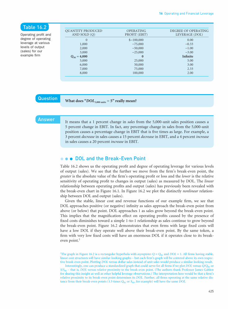
Question What does “DOL5,000 units = 5” really mean?

Answer It means that a 1 percent change in sales from the 5,000-unit sales position causes a 5 percent change in EBIT. In fact, any percentage change in sales from the 5,000-unitposition causes a percentage change in EBIT that is five times as large. For example, a 3 percent decrease in sales causes a 15 percent decrease in EBIT, and a 4 percent increasein sales causes a 20 percent increase in EBIT.

l l l DOL and the Break-Even PointTable 16.2 shows us the operating profit and degree of operating leverage for various levels of output (sales). We see that the further we move from the firm’s break-even point, thegreater is the absolute value of the firm’s operating profit or loss and the lower is the relativesensitivity of operating profit to changes in output (sales) as measured by DOL. The linearrelationship between operating profits and output (sales) has previously been revealed withthe break-even chart in Figure 16.1. In Figure 16.2 we plot the distinctly nonlinear relation-ship between DOL and output (sales).

Given the stable, linear cost and revenue functions of our example firm, we see that DOL approaches positive (or negative) infinity as sales approach the break-even point fromabove (or below) that point. DOL approaches 1 as sales grow beyond the break-even point.This implies that the magnification effect on operating profits caused by the presence of fixed costs diminishes toward a simple 1-to-1 relationship as sales continue to grow beyondthe break-even point. Figure 16.2 demonstrates that even firms with large fixed costs will have a low DOL if they operate well above their break-even point. By the same token, a firm with very low fixed costs will have an enormous DOL if it operates close to its break-even point.2

2The graph in Figure 16.2 is a rectangular hyperbola with asymptotes Q = QBE and DOL = 1. All firms having stable,linear cost structures will have similar-looking graphs – but each firm’s graph will be centered above its own respec-tive break-even point. Plotting DOL versus dollar sales instead of unit sales would produce a similar-looking result.

Interestingly, one can produce a standardized graph that could serve for all firms if we plot DOL versus Q/QBE orS/SBE – that is, DOL versus relative proximity to the break-even point. (The authors thank Professor James Gahlonfor sharing this insight as well as other helpful leverage observations.) The interpretation here would be that a firm’srelative proximity to its break-even point determines its DOL. Further, all firms operating at the same relative dis-tance from their break-even points (1.5 times QBE or SBE, for example) will have the same DOL.


425

••

Table 16.2Operating profit anddegree of operatingleverage at variouslevels of output(sales) for ourexample firm

QUANTITY PRODUCED OPERATING DEGREE OF OPERATINGAND SOLD (Q) PROFIT (EBIT) LEVERAGE (DOL)

0 $−100,000 0.001,000 −75,000 −0.332,000 −50,000 −1.003,000 −25,000 −3.00

QBE = 4,000 0 Infinite5,000 25,000 5.006,000 50,000 3.007,000 75,000 2.338,000 100,000 2.00

FUNO_C16.qxd 9/19/08 17:19 Page 425

Question How would knowledge of a firm’s DOL be of use to a financial manager?

Answer The manager would know in advance what impact a potential change in sales wouldhave on operating profit. Sometimes, in response to this advance knowledge, the firmmay decide to make some changes in its sales policy and/or cost structure. As a generalrule, firms do not like to operate under conditions of a high degree of operating leveragebecause, in that situation, a small drop in sales may lead to an operating loss.

l l l DOL and Business RiskIt is important to recognize that the degree of operating leverage is only one component of the overall business risk of the firm. The other principal factors giving rise to business risk are variability or uncertainty of sales and production costs. The firm’s degree of operatingleverage magnifies the impact of these other factors on the variability of operating profits.However, the degree of operating leverage itself is not the source of the variability. A highDOL means nothing if the firm maintains constant sales and a constant cost structure.Likewise, it would be a mistake to treat the degree of operating leverage of the firm as a synonym for its business risk. Because of the underlying variability of sales and productioncosts, however, the degree of operating leverage will magnify the variability of operatingprofits, and hence the company’s business risk. The degree of operating leverage should thus


426

••

Figure 16.2Plot of DOL versusquantity produced and sold, showing that closeness to the break-even point means highersensitivity ofoperating profits tochanges in quantityproduced and sold

Business risk Theinherent uncertainty in the physicaloperations of the firm.Its impact is shown in the variability of the firm’s operatingincome (EBIT).

FUNO_C16.qxd 9/19/08 17:19 Page 426


427

••

Indifference point(EBIT-EPS indifferencepoint) The level ofEBIT that producesthe same level of EPSfor two (or more)alternative capitalstructures.

be viewed as a measure of “potential risk” which becomes “active” only in the presence of salesand production cost variability.

Question Now that you have a better understanding of DOL, how can you tell from only theinformation in Frame A of Table 16.1 which firm – F, V, or 2F – will be more sensitiveto the anticipated 50 percent increase in sales for the next year?

Answer Simple. Calculate the DOL – using [(EBIT + FC)/EBIT] – for each firm, and then pickthe firm with the largest DOL.

Firm F: DOL$10,000 of sales = = 8

Firm V: DOL$11,000 of sales = = 2

Firm 2F: DOL$19,500 of sales = = 6.6

In short, Firm F – with a DOL of 8 – is most sensitive to the presence of operatingleverage. That is why a 50 percent increase in sales in the following year causes a 400 percent (8 × 50%) increase in operating profit.

Financial LeverageFinancial leverage involves the use of fixed cost financing. Interestingly, financial leverage isacquired by choice, but operating leverage sometimes is not. The amount of operating lever-age (the amount of fixed operating costs) employed by a firm is sometimes dictated by thephysical requirements of the firm’s operations. For example, a steel mill by way of its heavyinvestment in plant and equipment will have a large fixed operating cost component consist-ing of depreciation. Financial leverage, on the other hand, is always a choice item. No firm isrequired to have any long-term debt or preferred stock financing. Firms can, instead, financeoperations and capital expenditures from internal sources and the issuance of common stock.Nevertheless, it is a rare firm that has no financial leverage. Why, then, do we see such relianceon financial leverage?

Financial leverage is employed in the hope of increasing the return to common share-holders. Favorable or positive leverage is said to occur when the firm uses funds obtained at afixed cost (funds obtained by issuing debt with a fixed interest rate or preferred stock with aconstant dividend rate) to earn more than the fixed financing costs paid. Any profits left aftermeeting fixed financing costs then belong to common shareholders. Unfavorable or negativeleverage occurs when the firm does not earn as much as the fixed financing costs. The favor-ability of financial leverage, or “trading on the equity” as it is sometimes called, is judged interms of the effect that it has on earnings per share to the common shareholders. In effect,financial leverage is the second step in a two-step profit-magnification process. In step one,operating leverage magnifies the effect of changes in sales on changes in operating profit. Instep two, the financial manager has the option of using financial leverage to further magnifythe effect of any resulting changes in operating profit on changes in earnings per share. In thenext section we are interested in determining the relationship between earnings per share(EPS) and operating profit (EBIT) under various financing alternatives and the indifferencepoints between these alternatives.

$ , $ ,$ ,

2 500 14 0002 500+

$ , $ ,$ ,

2 000 2 0002 000

+

$ , $ ,$ ,

1000 7 0001000

+

FUNO_C16.qxd 9/19/08 17:19 Page 427

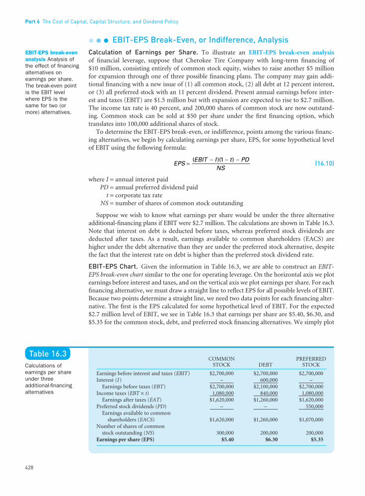
l l l EBIT-EPS Break-Even, or Indifference, AnalysisCalculation of Earnings per Share. To illustrate an EBIT-EPS break-even analysisof financial leverage, suppose that Cherokee Tire Company with long-term financing of $10 million, consisting entirely of common stock equity, wishes to raise another $5 millionfor expansion through one of three possible financing plans. The company may gain addi-tional financing with a new issue of (1) all common stock, (2) all debt at 12 percent interest,or (3) all preferred stock with an 11 percent dividend. Present annual earnings before inter-est and taxes (EBIT) are $1.5 million but with expansion are expected to rise to $2.7 million.The income tax rate is 40 percent, and 200,000 shares of common stock are now outstand-ing. Common stock can be sold at $50 per share under the first financing option, which translates into 100,000 additional shares of stock.

To determine the EBIT-EPS break-even, or indifference, points among the various financ-ing alternatives, we begin by calculating earnings per share, EPS, for some hypothetical levelof EBIT using the following formula:

(16.10)

where I = annual interest paidPD = annual preferred dividend paid

t = corporate tax rateNS = number of shares of common stock outstanding

Suppose we wish to know what earnings per share would be under the three alternativeadditional-financing plans if EBIT were $2.7 million. The calculations are shown in Table 16.3.Note that interest on debt is deducted before taxes, whereas preferred stock dividends arededucted after taxes. As a result, earnings available to common shareholders (EACS) arehigher under the debt alternative than they are under the preferred stock alternative, despitethe fact that the interest rate on debt is higher than the preferred stock dividend rate.

EBIT-EPS Chart. Given the information in Table 16.3, we are able to construct an EBIT-EPS break-even chart similar to the one for operating leverage. On the horizontal axis we plotearnings before interest and taxes, and on the vertical axis we plot earnings per share. For eachfinancing alternative, we must draw a straight line to reflect EPS for all possible levels of EBIT.Because two points determine a straight line, we need two data points for each financing alter-native. The first is the EPS calculated for some hypothetical level of EBIT. For the expected $2.7 million level of EBIT, we see in Table 16.3 that earnings per share are $5.40, $6.30, and$5.35 for the common stock, debt, and preferred stock financing alternatives. We simply plot

EPSEBIT I t PD

NS=

− − − ( )( ) 1


428

••

EBIT-EPS break-evenanalysis Analysis ofthe effect of financingalternatives onearnings per share.The break-even pointis the EBIT levelwhere EPS is thesame for two (ormore) alternatives.

Table 16.3Calculations ofearnings per shareunder threeadditional-financingalternatives

COMMON PREFERREDSTOCK DEBT STOCK

Earnings before interest and taxes (EBIT) $2,700,000 $2,700,000 $2,700,000Interest (I) – 600,000 –

Earnings before taxes (EBT) $2,700,000 $2,100,000 $2,700,000Income taxes (EBT × t) 1,080,000 840,000 1,080,000

Earnings after taxes (EAT) $1,620,000 $1,260,000 $1,620,000Preferred stock dividends (PD) – – 550,000

Earnings available to commonshareholders (EACS) $1,620,000 $1,260,000 $1,070,000

Number of shares of commonstock outstanding (NS) 300,000 200,000 200,000

Earnings per share (EPS) $5.40 $6.30 $5.35

FUNO_C16.qxd 9/19/08 17:19 Page 428

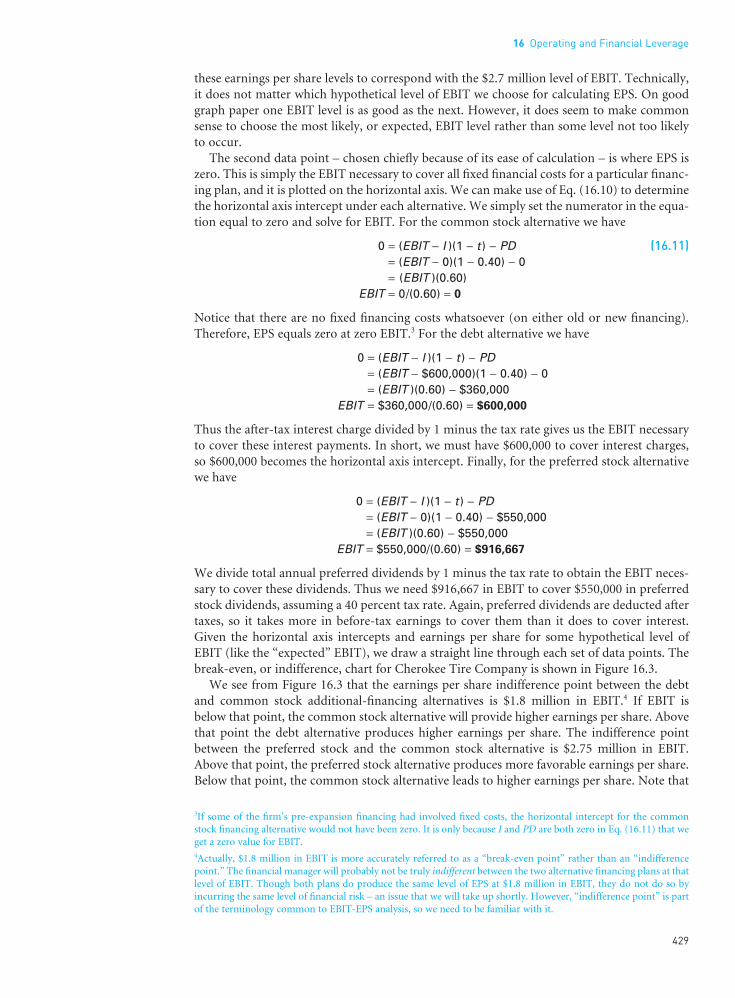
these earnings per share levels to correspond with the $2.7 million level of EBIT. Technically,it does not matter which hypothetical level of EBIT we choose for calculating EPS. On goodgraph paper one EBIT level is as good as the next. However, it does seem to make commonsense to choose the most likely, or expected, EBIT level rather than some level not too likelyto occur.

The second data point – chosen chiefly because of its ease of calculation – is where EPS iszero. This is simply the EBIT necessary to cover all fixed financial costs for a particular financ-ing plan, and it is plotted on the horizontal axis. We can make use of Eq. (16.10) to determinethe horizontal axis intercept under each alternative. We simply set the numerator in the equa-tion equal to zero and solve for EBIT. For the common stock alternative we have

0 = (EBIT − I )(1 − t ) − PD (16.11)= (EBIT − 0)(1 − 0.40) − 0= (EBIT )(0.60)

EBIT = 0/(0.60) = 0

Notice that there are no fixed financing costs whatsoever (on either old or new financing).Therefore, EPS equals zero at zero EBIT.3 For the debt alternative we have

0 = (EBIT − I )(1 − t ) − PD= (EBIT − $600,000)(1 − 0.40) − 0= (EBIT )(0.60) − $360,000

EBIT = $360,000/(0.60) = $600,000

Thus the after-tax interest charge divided by 1 minus the tax rate gives us the EBIT necessaryto cover these interest payments. In short, we must have $600,000 to cover interest charges,so $600,000 becomes the horizontal axis intercept. Finally, for the preferred stock alternativewe have

0 = (EBIT − I )(1 − t ) − PD= (EBIT − 0)(1 − 0.40) − $550,000= (EBIT )(0.60) − $550,000

EBIT = $550,000/(0.60) = $916,667

We divide total annual preferred dividends by 1 minus the tax rate to obtain the EBIT neces-sary to cover these dividends. Thus we need $916,667 in EBIT to cover $550,000 in preferredstock dividends, assuming a 40 percent tax rate. Again, preferred dividends are deducted aftertaxes, so it takes more in before-tax earnings to cover them than it does to cover interest.Given the horizontal axis intercepts and earnings per share for some hypothetical level ofEBIT (like the “expected” EBIT), we draw a straight line through each set of data points. Thebreak-even, or indifference, chart for Cherokee Tire Company is shown in Figure 16.3.

We see from Figure 16.3 that the earnings per share indifference point between the debtand common stock additional-financing alternatives is $1.8 million in EBIT.4 If EBIT is below that point, the common stock alternative will provide higher earnings per share. Abovethat point the debt alternative produces higher earnings per share. The indifference pointbetween the preferred stock and the common stock alternative is $2.75 million in EBIT.Above that point, the preferred stock alternative produces more favorable earnings per share.Below that point, the common stock alternative leads to higher earnings per share. Note that

3If some of the firm’s pre-expansion financing had involved fixed costs, the horizontal intercept for the commonstock financing alternative would not have been zero. It is only because I and PD are both zero in Eq. (16.11) that weget a zero value for EBIT.4Actually, $1.8 million in EBIT is more accurately referred to as a “break-even point” rather than an “indifferencepoint.” The financial manager will probably not be truly indifferent between the two alternative financing plans at thatlevel of EBIT. Though both plans do produce the same level of EPS at $1.8 million in EBIT, they do not do so byincurring the same level of financial risk – an issue that we will take up shortly. However, “indifference point” is partof the terminology common to EBIT-EPS analysis, so we need to be familiar with it.


429

••

FUNO_C16.qxd 9/19/08 17:19 Page 429

there is no indifference point between the debt and preferred stock alternatives. The debtalternative dominates for all levels of EBIT and by a constant amount of earnings per share,namely 95 cents.

Indifference Point Determined Mathematically. The indifference point between twoalternative financing methods can be determined mathematically by first using Eq. (16.10) to express EPS for each alternative and then setting these expressions equal to each other asfollows:

(16.12)

where EBIT1,2 = EBIT indifference point between the two alternative financing methods thatwe are concerned with – in this case, methods 1 and 2

I1, I2 = annual interest paid under financing methods 1 and 2PD1, PD2 = annual preferred stock dividend paid under financing methods 1 and 2

t = corporate tax rateNS1, NS2 = number of shares of common stock to be outstanding under financing

methods 1 and 2

Suppose that we wish to determine the indifference point between the common stock anddebt-financing alternatives in our example. We would have

Cross multiplying and rearranging, we obtain

(EBIT1,2)(0.60)(200,000) = (EBIT1,2)(0.60)(300,000) − (0.60)($600,000)(300,000)(EBIT1,2)(60,000) = $108,000,000,000

EBIT1,2 = $1,800,000

The EBIT-EPS indifference point, where earnings per share for the two methods of financingare the same, is $1.8 million. This amount can be verified graphically in Figure 16.3. Thusindifference points can be determined both graphically and mathematically.

Common Stock

EBIT

Debt

EBIT

( )( . ) ,

( $ , )( . )

,, ,1 2 1 20 1 0 40 0

300 000600 000 1 0 40 0

200 000− − −

=− − −

( )( )

( )( ) , ,EBIT I t PDNS

EBIT I t PDNS

1 2 1 1

1

1 2 2 2

2

1 1− − −=

− − −


430

••

Figure 16.3EBIT-EPS break-even,or indifference, chartfor three additional-financing alternatives

FUNO_C16.qxd 9/19/08 17:19 Page 430

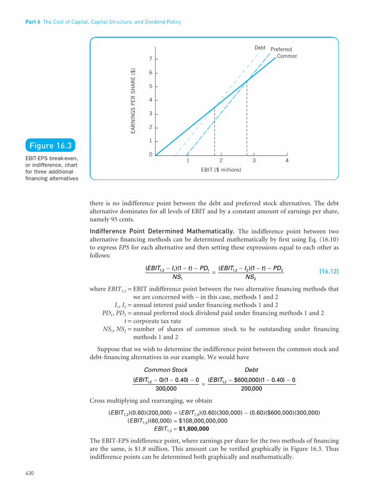
Effect on Risk. So far our concern with EBIT-EPS analysis has been only with what happensto the return to common shareholders as measured by earnings per share. We have seen inour example that, if EBIT is above $1.8 million, debt financing is the preferred alternativefrom the standpoint of earnings per share. We know from our earlier discussion, however,that the impact on expected return is only one side of the coin. The other side is the effect thatfinancial leverage has on risk. An EBIT-EPS chart does not permit a precise analysis of risk.Nevertheless, certain generalizations are possible. For one thing, the financial manager shouldcompare the indifference point between two alternatives, such as debt financing versus com-mon stock financing, with the most likely level of EBIT. The higher the expected level of EBIT,assuming that it exceeds the indifference point, the stronger the case that can be made for debtfinancing, all other things the same.

In addition, the financial manager should assess the likelihood of future EBITs actuallyfalling below the indifference point. As before, our estimate of expected EBIT is $2.7 million.Given the business risk of the company and the resulting possible fluctuations in EBIT, thefinancial manager should assess the probability of EBITs falling below $1.8 million. If theprobability is negligible, the use of the debt alternative will be supported. On the other hand,if EBIT is presently only slightly above the indifference point and the probability of EBITsfalling below this point is high, the financial manager may conclude that the debt alternativeis too risky.

This notion is illustrated in Figure 16.4, where two probability distributions of possibleEBITs are superimposed on the indifference chart first shown in Figure 16.3. In Figure 16.4,however, we focus on only the debt and common stock alternatives. For the safe (peaked) dis-tribution, there is virtually no probability that EBIT will fall below the indifference point.Therefore we might conclude that debt should be used, because the effect on shareholderreturn is substantial, whereas risk is negligible. For the risky (flat) distribution, there is asignificant probability that EBIT will fall below the indifference point. In this case, the finan-cial manager may conclude that the debt alternative is too risky.

In summary, the greater the level of expected EBIT above the indifference point and thelower the probability of downside fluctuation, the stronger the case that can be made for the


431

••

Figure 16.4EBIT-EPS break-even,or indifference, chartand EBIT probabilitydistributions for debtand common stockadditional-financingalternatives

FUNO_C16.qxd 9/19/08 17:19 Page 431

use of debt financing. EBIT-EPS break-even analysis is but one of several methods used fordetermining the appropriate amount of debt a firm might carry. No one method of analysisis satisfactory by itself. When several methods of analysis are undertaken simultaneously,however, generalizations are possible.

l l l Degree of Financial Leverage (DFL)

A quantitative measure of the sensitivity of a firm’s earnings per share to a change in the firm’soperating profit is called the degree of financial leverage (DFL). The degree of financial lever-age at a particular level of operating profit is simply the percentage change in earnings pershare over the percentage change in operating profit that causes the change in earnings per share. Thus,

(16.13)

Whereas Eq. (16.13) is useful for defining DFL, a simple alternative formula derived fromEq. (16.13) is more useful for actually computing DFL values:

(16.14)

Equation (16.14) states that DFL at a particular level of operating profit is calculated by divid-ing operating profit by the dollar difference between operating profit and the amount ofbefore-tax operating profit necessary to cover total fixed financing costs. (Remember, it takesmore in before-tax earnings to cover preferred dividends than it does to cover interest: hencewe need to divide preferred dividends by 1 minus the tax rate in our formula.)

For our example firm, using the debt-financing alternative at $2.7 million in EBIT, we have

For the preferred stock financing alternative, the degree of financial leverage is

Interestingly, although the stated fixed cost involved with the preferred stock financing alter-native is lower than that for the debt alternative ($550,000 versus $600,000), the DFL is greaterunder the preferred stock option than under the debt option. This is because of the taxdeductibility of interest and the nondeductibility of preferred dividends. It is often argued thatpreferred stock financing is of less risk than debt financing for the issuing firm. With regardto the risk of cash insolvency, this is probably true. But the DFL tells us that the relative vari-ability of EPS will be greater under the preferred stock financing arrangement, everything elsebeing equal. This discussion naturally leads us to the topic of financial risk and its relation-ship to the degree of financial leverage.

l l l DFL and Financial Risk

Financial Risk. Broadly speaking, financial risk encompasses both the risk of possible insol-vency and the added variability in earnings per share that is induced by the use of financialleverage. As a firm increases the proportion of fixed cost financing in its capital structure,fixed cash outflows increase. As a result, the probability of cash insolvency increases. To illustrate this aspect of financial risk, suppose that two firms differ with respect to financial

DFLEBIT of $2.7 million =−

= $ , ,

$ , , [$ , /( . )]

2 700 0002 700 000 550 000 0 60

1.51

DFLEBIT of $2.7 million =−

= $ , ,

$ , , $ ,

2 700 0002 700 000 600 000

1.29

DFLEBIT

EBIT I PD tEBIT X of dollars =− − −

[ /( )]1

Degree of financialleverage (DFL) at EBIT of

dollars

Percentage change inearnings per share (EPS)

Percentage change inoperating profit (EBIT)

X =


432

••

Degree of financialleverage (DFL) Thepercentage change in a firm’s earningsper share (EPS)resulting from a 1percent change inoperating profit (EBIT).

Cash insolvencyInability to payobligations as they fall due.

Financial risk Theadded variability inearnings per share(EPS) – plus the riskof possible insolvency– that is induced bythe use of financialleverage.

FUNO_C16.qxd 9/19/08 17:19 Page 432

leverage but are identical in every other respect. Each has expected annual cash earningsbefore interest and taxes of $80,000. Firm A has no debt. Firm B has $200,000 worth of 15 per-cent perpetual bonds outstanding. Thus the total annual fixed financial charges for Firm B are$30,000, whereas Firm A has no fixed financial charges. If cash earnings for both firms hap-pen to be 75 percent lower than expected, namely $20,000, firm B will be unable to cover itsfinancial charges with cash earnings. We see, then, that the probability of cash insolvencyincreases with the financial charges incurred by the firm.

The second aspect of financial risk involves the relative dispersion of earnings per share. Toillustrate, suppose that the expected future EBITs for firm A and firm B are random variableswhere the expected values of the probability distributions are each $80,000 and the standarddeviations $40,000. As before, firm A has no debt but rather 4,000 shares of $10-par-valuecommon stock outstanding. Firm B has $200,000 in 15 percent bonds and 2,000 shares of $10-par-value common stock outstanding.

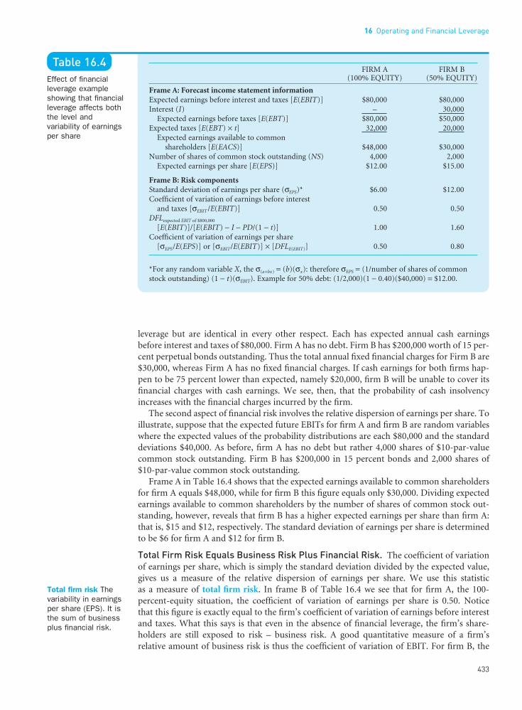
Frame A in Table 16.4 shows that the expected earnings available to common shareholdersfor firm A equals $48,000, while for firm B this figure equals only $30,000. Dividing expectedearnings available to common shareholders by the number of shares of common stock out-standing, however, reveals that firm B has a higher expected earnings per share than firm A:that is, $15 and $12, respectively. The standard deviation of earnings per share is determinedto be $6 for firm A and $12 for firm B.

Total Firm Risk Equals Business Risk Plus Financial Risk. The coefficient of variationof earnings per share, which is simply the standard deviation divided by the expected value,gives us a measure of the relative dispersion of earnings per share. We use this statistic as a measure of total firm risk. In frame B of Table 16.4 we see that for firm A, the 100-percent-equity situation, the coefficient of variation of earnings per share is 0.50. Notice that this figure is exactly equal to the firm’s coefficient of variation of earnings before interestand taxes. What this says is that even in the absence of financial leverage, the firm’s share-holders are still exposed to risk – business risk. A good quantitative measure of a firm’s relative amount of business risk is thus the coefficient of variation of EBIT. For firm B, the


433

••

Table 16.4Effect of financialleverage exampleshowing that financialleverage affects boththe level andvariability of earningsper share

FIRM A FIRM B(100% EQUITY) (50% EQUITY)

Frame A: Forecast income statement informationExpected earnings before interest and taxes [E(EBIT)] $80,000 $80,000Interest (I) – 30,000

Expected earnings before taxes [E(EBT)] $80,000 $50,000Expected taxes [E(EBT) × t] 32,000 20,000

Expected earnings available to commonshareholders [E(EACS)] $48,000 $30,000

Number of shares of common stock outstanding (NS) 4,000 2,000Expected earnings per share [E(EPS)] $12.00 $15.00

Frame B: Risk componentsStandard deviation of earnings per share (σEPS)* $6.00 $12.00Coefficient of variation of earnings before interest

and taxes [σEBIT /E(EBIT)] 0.50 0.50DFLexpected EBIT of $800,000

[E(EBIT)]/[E(EBIT) − I − PD/(1 − t)] 1.00 1.60Coefficient of variation of earnings per share

[σEPS/E(EPS)] or [σEBIT/E(EBIT)] × [DFLE(EBIT)] 0.50 0.80

*For any random variable X, the σ(a+bx) = (b)(σx): therefore σEPS = (1/number of shares of commonstock outstanding) (1 − t)(σEBIT). Example for 50% debt: (1/2,000)(1 − 0.40)($40,000) = $12.00.

Total firm risk Thevariability in earningsper share (EPS). It isthe sum of businessplus financial risk.

FUNO_C16.qxd 9/19/08 17:19 Page 433

50-percent-debt situation, the coefficient of variation of earnings per share is 0.80. Becausefirm B is exactly like firm A except for the use of financial leverage, we can use the differencebetween the coefficients of variation of earnings per share for firm B and firm A: that is, 0.80 − 0.50 = 0.30, as a measure of the added variability in earnings per share for firm B that is induced by the use of leverage; in short, this difference is a measure of financial risk.Equivalently, this measure of financial risk equals the difference between firm B’s coefficientof variation of earnings per share and its coefficient of variation of earnings before interestand taxes.

Take Note

In summary, then

l Total firm risk = business risk + financial risk.

l The coefficient of variation of earnings per share, CVEPS, is a measure of relative total firmrisk : CVEPS = σEPS /E(EPS).

l The coefficient of variation of earnings before interest and taxes, CVEBIT, is a measure ofrelative business risk: CVEBIT = σEBIT /E(EBIT).

l The difference, therefore, between the coefficient of variation of earnings per share(CVEPS) and the coefficient of variation of earnings before interest and taxes (CVEBIT) is ameasure of relative financial risk: (CVEPS − CVEBIT).

We have seen from Table 16.4 that total firm risk in our example, as measured by thecoefficient of variation of earnings per share, is higher under the 50-percent-bond financingthan it is under the 100-percent-equity financing. However, the expected level of earnings pershare is also higher. We witness, once again, the kind of risk-return trade-off that character-izes most financial leverage decisions.

DFL Magnifies Risk. Our measure of relative total firm risk, the coefficient of variation ofearnings per share, can be calculated directly by dividing the standard deviation of earningsper share by the expected earnings per share. However, given the assumptions behind ourexample, it can be shown that this measure is also equal to the coefficient of variation of earn-ings before interest and taxes times the degree of financial leverage at the expected EBIT level.5

Firm A, in our example, has no financial leverage and a resulting DFL equal to 1: in short,there is no magnification of business risk as measured by the CVEBIT. For firm A, then, CVEPS

equals CVEBIT, and thus its total firm risk is equal to its business risk. Firm B’s CVEPS, on theother hand, is equal to its CVEBIT (its measure of business risk) times 1.6 (its DFL at theexpected EBIT). Thus, for firms employing financial leverage, their DFL will act to magnifythe impact of business risk on the variability of earnings per share. So, although DFL is notsynonymous with financial risk, its magnitude does determine the relative amount of addi-tional risk induced by the use of financial leverage. As a result, firms with high business riskwill often employ a financing mix that entails a limited DFL, and vice versa.

5Proof:


434

••

FUNO_C16.qxd 9/19/08 17:19 Page 434

Total LeverageWhen financial leverage is combined with operating leverage, the result is referred to as total(or combined) leverage. The effect of combining financial and operating leverage is a two-step magnification of any change in sales into a larger relative change in earnings per share. Aquantitative measure of this total sensitivity of a firm’s earnings per share to a change in thefirm’s sales is called the degree of total leverage (DTL).

l l l Degree of Total Leverage (DTL)

The degree of total leverage of a firm at a particular level of output (or sales) is equal to thepercentage change in earnings per share over the percentage change in output (or sales) thatcauses the change in earnings per share. Thus,

(16.15)

Computationally, we can make use of the fact that the degree of total leverage is simply theproduct of the degree of operating leverage and the degree of financial leverage as follows:

DTLQ units (or S dollars) = DOLQ units (or S dollars) × DFLEBIT of X dollars (16.16)

In addition, multiplying alternative DOLs, Eqs. (16.8) and (16.9), by DFL, Eq. (16.14), gives us

(16.17)

(16.18)

These alternative equations tell us that for a particular firm the greater the before-tax financialcosts, the greater the degree of total leverage over what it would be in the absence of financialleverage.

Suppose that our bicycle-helmet manufacturing firm used to illustrate operating leveragehas $200,000 in debt at 8 percent interest. Recall that the selling price is $50 a unit, variableoperating costs are $25 a unit, and annual fixed operating costs are $100,000. Assume that thetax rate is 40 percent, and that we wish to determine the degree of total leverage at 8,000 unitsof production and sales. Therefore, using Eq. (16.17), we have

Thus a 10 percent increase in the number of units produced and sold would result in a 23.8percent increase in earnings per share.

Stating the degree of total leverage for our example firm in terms of the product of itsdegree of operating leverage times its degree of financial leverage, we get

In the absence of financial leverage, our firm’s degree of total leverage would have been equal to its degree of operating leverage for a value of 2 (remember, DFL for a firm with no

DOL DFL DTL8,000 units EBIT of $100,000 8,000 units

8 000 50 258 000 50 25 100 000

100 000100 000 16 000

, ($ $ ), ($ $ ) $ ,

$ ,

$ , $ ,

−− −

×

×

×

−

=

=

=2.00 1.19

2.38

2.38

DTL8,000 units =−

− − −=

, ($ $ ), ($ $ ) $ , $ ,

8 000 50 25

8 000 50 25 100 000 16 0002.38

DTLEBIT FC

EBIT I PD tS dollars of sales =+

− − −

[ /( )]1

DTLQ P V

Q P V FC I PD tQ ( )

( ) [ /( )]units =−

− − − − −1

Degree of total leverage (DTL)at units (or dollars)


Percentage change inearnings per share (EPS)

Percentage change inoutput (or sales)

Q S =


435

••

Total (or combined)leverage The use ofboth fixed operatingand financing costs bythe firm.

Degree of totalleverage (DTL) Thepercentage change ina firm’s earnings pershare (EPS) resultingfrom a 1 percentchange in output(sales). This is alsoequal to a firm’sdegree of operatingleverage (DOL) timesits degree of financialleverage (DFL) at aparticular level ofoutput (sales).

FUNO_C16.qxd 9/19/08 17:19 Page 435

financial leverage equals 1). We see, however, that the firm’s financial leverage magnifies itsDOL figure by a factor of 1.19 to produce a degree of total leverage equal to 2.38.

l l l DTL and Total Firm RiskOperating leverage and financial leverage can be combined in a number of different ways toobtain a desirable degree of total leverage and level of total firm risk. High business risk canbe offset with low financial risk and vice versa. The proper overall level of firm risk involves atrade-off between total firm risk and expected return. This trade-off must be made in keepingwith the objective of maximizing shareholder value. The discussion, so far, is meant to showhow certain tools can be employed to provide information on the two types of leverage –operating and financial – and their combined effect.

Cash-Flow Ability to Service DebtWhen trying to determine the appropriate financial leverage for a firm, we would also analyzethe cash-flow ability of the firm to service fixed financial charges. The greater the dollaramount of senior securities that the firm issues and the shorter their maturity, the greater thefixed financial charges of the firm. These charges include principal and interest payments ondebt, financial lease payments, and preferred stock dividends. Before taking on additionalfixed financial charges, the firm should analyze its expected future cash flows, because fixedfinancial charges must be met with cash. The inability to meet these charges, with the excep-tion of preferred stock dividends, may result in financial insolvency. The greater and morestable the expected future cash flows of the firm, the greater the debt capacity of the company.

l l l Coverage RatiosAmong the ways in which we can gain knowledge about the debt capacity of a firm is throughan analysis of coverage ratios. These ratios, as you may remember from Chapter 6, aredesigned to relate the financial charges of a firm to the firm’s ability to service, or cover, them.In the computation of these ratios, one typically uses earnings before interest and taxes as arough measure of the cash flow available to cover fixed financial charges. Perhaps the mostwidely used coverage ratio is the interest coverage ratio, or times interest earned. This ratio issimply earnings before interest and taxes for a particular period divided by interest charges forthe period:

(16.19)

Suppose, for example, that the most recent annual earnings before interest and taxes for acompany were $6 million and annual interest payments on all debt obligations were $1.5 million.Then EBIT would “cover” interest charges four times. This tells us that EBIT can drop by asmuch as 75 percent and the firm will still be able to cover interest payments out of earnings.

An interest coverage ratio of only 1 indicates that earnings are just sufficient to satisfy theinterest burden. Generalizations about what is a proper interest coverage ratio are inappro-priate unless reference is made to the type of business in which the firm is engaged. In a highlystable business, a relatively low interest coverage ratio may be appropriate, whereas it may notbe appropriate in a highly cyclical business.

Note that the interest coverage ratio tells us nothing about the firm’s ability to meet prin-cipal payments on its debts. The inability to meet a principal payment constitutes the samelegal default as failure to meet an interest payment. Therefore it is useful to compute the coverage ratio for the full debt-service burden. This ratio is

Interest coverage ratio(or times interest earned)

Earnings before interestand taxes (EBIT)Interest expense

=


436

••

Debt capacity Themaximum amount ofdebt (and other fixed-charge financing) thata firm can adequatelyservice.

Coverage ratiosRatios that relate thefinancial charges of afirm to its ability toservice, or cover,them.

Interest coverageratio Earnings beforeinterest and taxesdivided by interestcharges. It indicates afirm’s ability to coverinterest charges. It isalso called timesinterest earned.

Debt-service burdenCash required duringa specific period,usually a year, tomeet interestexpenses andprincipal payments.Also called simplydebt service.

FUNO_C16.qxd 9/19/08 17:19 Page 436

(16.20)

Here principal payments are adjusted upward for the tax effect. The reason is that EBIT rep-resents earnings before tax. Because principal payments are not deductible for tax purposes,they must be paid out of after-tax earnings. Therefore we must adjust principal payments sothat they are consistent with EBIT. If principal payments in our previous example were $1million per annum and the tax rate were 40 percent, the debt-service coverage ratio would be

A coverage ratio of 1.89 means that EBIT can fall by only 47 percent before earnings coverageis insufficient to service the debt.6 Obviously, the closer the debt-service coverage ratio is to 1,the worse things are, all other things the same. However, even with this coverage ratio beingless than 1, a company may still be able to meet its obligations if it can renew some of its debtwhen principal comes due or if assets are sold.

Part of the overall analysis of the financial risk associated with financial leverage shouldfocus on the firm’s ability to service total fixed charges. Lease financing is not debt per se, butits impact on cash flows is exactly the same as the payment of interest and principal on a debtobligation. (See Chapter 21 for an analysis of lease financing.) Annual financial lease pay-ments, therefore, should be added to the numerator and denominator of Eq. (16.20) in orderto properly reflect the total cash-flow burden associated with financing.

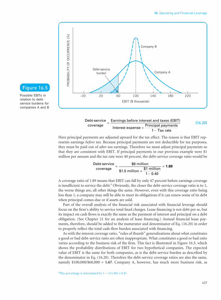
As with the interest coverage ratio, “rules of thumb” generalizations about what constitutesa good or bad debt-service ratio are often inappropriate. What constitutes a good or bad ratiovaries according to the business risk of the firm. This fact is illustrated in Figure 16.5, whichshows the probability distributions of EBIT for two hypothetical companies. The expectedvalue of EBIT is the same for both companies, as is the debt-service burden as described bythe denominator in Eq. (16.20). Therefore the debt-service coverage ratios are also the same,namely $100,000/$60,000 = 1.67. Company A, however, has much more business risk, as

Debt-servicecoverage

$6 million

$1.5 million $1 million

0

.

=+

−

=

1 40

1.89

Debt-servicecoverage

Earnings before interest and taxes (EBIT)

Interest expense Principal payments

Tax rate

=+

−1

6This percentage is determined by 1 − (1/1.89) = 0.47.


437

••

Figure 16.5Possible EBITs inrelation to debt-service burdens forcompanies A and B

FUNO_C16.qxd 9/19/08 17:19 Page 437

shown in the greater variability of its EBIT. The probability that EBIT will fall below the debt-service burden is depicted by the shaded areas in the figure. We see that this probabilityis much greater for company A than it is for company B. Though a debt-service coverage ratio of 1.67 may be appropriate for company B, it may not be appropriate for company A.Simply put, a company with stable cash flows is better able to take on relatively more fixedcharges.

Ultimately, one wants to make generalizations about the appropriate amount of debt (andleases) for a firm to have in its financing mix. It is clear that the ability of a going-concern firmto service debt over the long run is tied to earnings. Therefore coverage ratios are an import-ant tool of analysis. However, they are but one tool by which a person is able to reach con-clusions with respect to determining an appropriate financing mix for the firm. Coverageratios, like all ratios, are subject to certain limitations and, consequently, cannot be used as asole means for determining a firm’s financing. The fact that EBIT falls below the debt-serviceburden does not spell immediate doom for the company. Often alternative sources of funds,including renewal of the loan, are available, and these sources must be considered.

l l l Probability of Cash InsolvencyThe vital question for the firm is not so much whether a coverage ratio will fall below 1 butrather, what are the chances of cash insolvency? Fixed-charge financing adds to the firm’s danger of cash insolvency. Therefore the answer depends on whether all sources of payment– earnings, cash, a new financing arrangement, or the sale of assets – are collectively deficient.A coverage ratio tells only part of the story. To address the broad question of cash insolvency,we must obtain information on the possible deviation of actual cash flows from those that areexpected. As we discussed in Chapter 7, cash budgets can be prepared for a range of possibleoutcomes, with a probability attached to each outcome. This information is extremely valu-able to the financial manager in evaluating the ability of the firm to meet fixed obligations.Not only are expected earnings taken into account in determining this ability, but other cash-flow factors as well – the purchase or sale of assets, the liquidity of the firm, dividendpayments, and seasonal patterns. Given the probabilities of particular cash-flow sequences,the financial manager is able to determine the amount of fixed financing charges the companycan undertake while still remaining within insolvency limits tolerable to management.

Management may feel that a 5 percent probability of being out of cash is the maximum that it can tolerate and that this probability corresponds to a cash budget prepared under pessimistic assumptions. In this case, debt might be undertaken up to the point where thecash balance under the pessimistic cash budget is just sufficient to cover the fixed chargesassociated with the debt. In other words, debt would be increased to the point at which theadditional cash drain would cause the probability of cash insolvency to equal the risk toler-ance specified by management. Note that the method of analysis simply provides a means forassessing the effect of increases in debt on the risk of cash insolvency. On the basis of thisinformation, management would arrive at the most appropriate level of debt.

The analysis of the cash-flow ability of the firm to service fixed financial charges is perhapsthe best way to analyze financial risk, but there is a real question as to whether all (or most)of the participants in the financial markets analyze a company in this manner. Sophisticatedlenders and institutional investors certainly analyze the amount of fixed financial charges andevaluate financial risk in keeping with the ability of the firm to service these charges. However,individual investors may judge financial risk more by book value proportions of debt andequity. There may or may not be a reasonable correspondence between the ratio of debt toequity and the amount of fixed charges relative to the firm’s cash-flow ability to service thesecharges. Some firms may have relatively high ratios of debt to equity but substantial cash-flowability to service debt. Consequently, the analysis of debt-to-equity ratios alone can be deceiv-ing, and an analysis of the magnitude and stability of cash flows relative to fixed financialcharges is extremely important in determining the appropriate financing mix for the firm.


438

••

FUNO_C16.qxd 9/19/08 17:19 Page 438

Other Methods of Analysis

l l l Comparison of Capital Structure RatiosAnother method of analyzing the appropriate financing mix for a company is to evaluate thecapital structure of other companies having similar business risk. Companies used in thiscomparison are most often those in the same industry. If the firm is contemplating a capitalstructure significantly out of line with that of similar companies, it is conspicuous in the marketplace. This is not to say that the firm is wrong. Other companies in the industry maybe too conservative in their use of debt. The optimal capital structure for all companies in theindustry might call for a higher proportion of debt to equity than the industry average. As aresult, the firm may be able to justify more debt than the industry average. If the firm’s finan-cial leverage is noticeably out of line in either direction, it should be prepared to justify itsposition, because investment analysts and creditors tend to evaluate companies by industry.

There are wide variations in the use of financial leverage across business firms. A good dealof the variation is removed, however, if one groups firms by industry classification, becausethere is a tendency for the firms in an industry to cluster when it comes to debt ratios. Forselected industries, the debt-to-net-worth ratios for a recent period looked as follows:

INDUSTRY DEBT TO NET WORTH

Optical instruments and lenses (manufacturing) 1.2Pharmaceutical preparations (manufacturing) 1.2Meat packing plants (manufacturing) 1.8Electronic components (manufacturing) 1.8Carpets and rugs (manufacturing) 1.9Wood kitchen cabinets (manufacturing) 2.9Gasoline service stations (retail) 3.2General contractors (single-family houses) 5.0

Whereas optical instruments manufacturers and pharmaceutical companies do not employmuch financial leverage, general contractors make extensive use of debt in financing projects.So when making capital structure comparisons, look at other companies in the same indus-try. In short, compare apples with apples as opposed to apples with oranges.

l l l Surveying Investment Analysts and LendersThe firm may profit by also talking with investment analysts, institutional investors, andinvestment bankers to obtain their views on appropriate amounts of financial leverage. Theseanalysts examine many companies and are in the business of recommending stocks. Theytherefore have an influence on the financial market. Their judgments with respect to how themarket evaluates financial leverage may be very worthwhile. Similarly, a firm may wish tointerview lenders to see how much debt it can undertake before the cost of borrowing is likelyto rise. Finally, the management of a company may develop a “feel” for what has happened tothe market price of the company’s stock when it has issued debt in the past.

l l l Security RatingsThe financial manager must consider the effect of a financing alternative on its security rat-ing. Whenever a company sells a debt or preferred stock issue to public investors, as opposedto private lenders such as banks, it must have the issue rated by one or more rating services.The principal rating agencies are Moody’s Investors Service and Standard & Poor’s. The issuerof a new corporate security issue contracts with the agency to evaluate the issue as to quality,as well as to update the rating throughout the issue’s life. For this service, the issuer pays a fee. In addition, the rating agency charges subscribers to its rating publications. Whereas the


439

••

Capital structure Themix (or proportion) ofa firm’s permanentlong-term financingrepresented by debt,preferred stock, andcommon stock equity.

FUNO_C16.qxd 9/19/08 17:19 Page 439

assignment of a rating for a new issue is current, changes in ratings of existing securities tendto lag the events that prompt the changes.

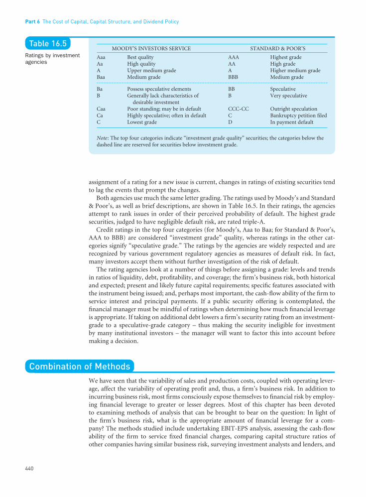
Both agencies use much the same letter grading. The ratings used by Moody’s and Standard& Poor’s, as well as brief descriptions, are shown in Table 16.5. In their ratings, the agenciesattempt to rank issues in order of their perceived probability of default. The highest gradesecurities, judged to have negligible default risk, are rated triple-A.

Credit ratings in the top four categories (for Moody’s, Aaa to Baa; for Standard & Poor’s,AAA to BBB) are considered “investment grade” quality, whereas ratings in the other cat-egories signify “speculative grade.” The ratings by the agencies are widely respected and arerecognized by various government regulatory agencies as measures of default risk. In fact,many investors accept them without further investigation of the risk of default.

The rating agencies look at a number of things before assigning a grade: levels and trendsin ratios of liquidity, debt, profitability, and coverage; the firm’s business risk, both historicaland expected; present and likely future capital requirements; specific features associated withthe instrument being issued; and, perhaps most important, the cash-flow ability of the firm toservice interest and principal payments. If a public security offering is contemplated, thefinancial manager must be mindful of ratings when determining how much financial leverageis appropriate. If taking on additional debt lowers a firm’s security rating from an investment-grade to a speculative-grade category – thus making the security ineligible for investment by many institutional investors – the manager will want to factor this into account beforemaking a decision.

Combination of MethodsWe have seen that the variability of sales and production costs, coupled with operating lever-age, affect the variability of operating profit and, thus, a firm’s business risk. In addition toincurring business risk, most firms consciously expose themselves to financial risk by employ-ing financial leverage to greater or lesser degrees. Most of this chapter has been devoted to examining methods of analysis that can be brought to bear on the question: In light of the firm’s business risk, what is the appropriate amount of financial leverage for a com-pany? The methods studied include undertaking EBIT-EPS analysis, assessing the cash-flowability of the firm to service fixed financial charges, comparing capital structure ratios of other companies having similar business risk, surveying investment analysts and lenders, and


440

••

Table 16.5Ratings by investmentagencies

MOODY’S INVESTORS SERVICE STANDARD & POOR’S

Aaa Best quality AAA Highest gradeAa High quality AA High gradeA Upper medium grade A Higher medium gradeBaa Medium grade BBB Medium grade

Ba Possess speculative elements BB SpeculativeB Generally lack characteristics of B Very speculative

desirable investmentCaa Poor standing; may be in default CCC-CC Outright speculationCa Highly speculative; often in default C Bankruptcy petition filedC Lowest grade D In payment default

Note: The top four categories indicate “investment grade quality” securities; the categories below thedashed line are reserved for securities below investment grade.

FUNO_C16.qxd 9/19/08 17:19 Page 440

evaluating the effect of a financial leverage decision on a firm’s security rating. In addition tothe information provided by using these techniques, the financial manager will want to knowthe changing interest costs for various levels of debt. The maturity structure of debt is impor-tant as well, but we take this up later in the book. We focus here only on the broad issue of theamount of financial leverage to employ. All of the analyses should be guided by the concep-tual framework presented in the next chapter.

The implicit cost of financial leverage – that is, the effect that financial leverage has on thevalue of the firm’s common stock – is not easy to isolate and determine. Nevertheless, byundertaking a variety of analyses, the financial manager should be able to determine, withinsome range, the appropriate capital structure for the firm. By necessity, the final decision hasto be somewhat subjective, but it should be based on the best information available. In thisway, the firm is able to obtain the capital structure most appropriate for its situation – the oneit hopes will maximize the market price of the firm’s common stock.

Key Learning Points

l Leverage refers to the use of fixed costs in an attemptto increase (or lever up) profitability. Operating lever-age is due to fixed operating costs associated with theproduction of goods or services, whereas financialleverage is due to the existence of fixed financing costs– in particular, interest on debt. Both types of leverageaffect the level and variability of the firm’s after-taxearnings, and hence the firm’s overall risk and return.

l We can study the relationship between total operatingcosts and total revenues by using a break-even chart,which shows the relationship among total revenues,total operating costs, and operating profits for variouslevels of production and sales.

l The break-even point is the sales volume required sothat total revenues and total costs are equal. It may beexpressed in units or in sales dollars.

l A quantitative measure of the sensitivity of a firm’soperating profit to a change in the firm’s sales is calledthe degree of operating leverage (DOL). The DOL of afirm at a particular level of output (or sales) is the per-centage change in operating profit over the percentagechange in output (or sales) that causes the change inprofits. The closer a firm operates to its break-evenpoint, the higher is the absolute value of its DOL.

l The degree of operating leverage contributes but onecomponent of the overall business risk of the firm.The other principal factors giving rise to business riskare variability or uncertainty of sales and produc-tion costs. The firm’s degree of operating leveragemagnifies the impact of these other factors on thevariability of operating profits.

l Financial leverage is the second step in a two-step profit-magnification process. In step one, operating leveragemagnifies the effect of changes in sales on changes inoperating profit. In step two, financial leverage can be

used to further magnify the effect of any resulting changesin operating profit on changes in earnings per share.

l EBIT-EPS break-even, or indifference, analysis is usedto study the effect of financing alternatives on earn-ings per share. The break-even point is the EBIT levelwhere EPS is the same for two (or more) alternatives.The higher the expected level of EBIT, assuming thatit exceeds the indifference point, the stronger the casethat can be made for debt financing, all other thingsthe same. In addition, the financial manager shouldassess the likelihood of future EBITs actually fallingbelow the indifference point.

l A quantitative measure of the sensitivity of a firm’searnings per share to a change in the firm’s operatingprofit is called the degree of financial leverage (DFL).The DFL at a particular level of operating profit is the percentage change in earnings per share over thepercentage change in operating profit that causes thechange in earnings per share.

l Financial risk encompasses both the risk of possibleinsolvency and the “added” variability in earnings pershare that is induced by the use of financial leverage.

l When financial leverage is combined with operatingleverage, the result is referred to as total (or combined)leverage. A quantitative measure of the total sensitivityof a firm’s earnings per share to a change in the firm’ssales is called the degree of total leverage (DTL). TheDTL of a firm at a particular level of output (or sales)is equal to the percentage change in earnings per shareover the percentage change in output (or sales) thatcauses the change in earnings per share.

l When trying to determine the appropriate financialleverage for a firm, the cash-flow ability of the firm to service debt should be evaluated. The firm’s debtcapacity can be assessed by analyzing coverage ratios


441

••

FUNO_C16.qxd 9/19/08 17:19 Page 441

Questions

1. Define operating leverage and the degree of operating leverage (DOL). How are the tworelated?

2. Classify the following short-run manufacturing costs as either typically fixed or typicallyvariable. Which costs are variable at management’s discretion? Are any of these costs fixedin the long run?a. Insurance d. R&D g. Depletionb. Direct labor e. Advertising h. Depreciationc. Bad-debt loss f. Raw materials i. Maintenance

3. What would be the effect on the firm’s operating break-even point of the following individual changes?a. An increase in selling priceb. An increase in the minimum wage paid to the firm’s employeesc. A change from straight-line to accelerated depreciationd. Increased salese. A liberalized credit policy to customers

4. Are there any businesses that are risk free?5. Your friend, Jacques Fauxpas, suggests, “Firms with high fixed operating costs show

extremely dramatic fluctuations in operating profits for any given change in sales volume.” Do you agree with Jacques? Why or why not?

6. You can have a high degree of operating leverage (DOL) and still have low business risk.Why? By the same token, you can have a low DOL and still have high business risk. Why?

7. Define financial leverage and the degree of financial leverage (DFL). How are the tworelated?

8. Discuss the similarities and differences between financial leverage and operating leverage.9. Can the concept of financial leverage be analyzed quantitatively? Explain.

10. The EBIT-EPS chart suggests that the higher the debt ratio, the higher are the earningsper share for any level of EBIT above the indifference point. Why do firms sometimeschoose financing alternatives that do not maximize EPS?

11. Why is the percentage of debt for an electric utility higher than that for the typical manu-facturing company?

12. Is the debt-to-equity ratio a good proxy for financial risk as represented by the cash-flowability of a company to service debt? Why or why not?

13. How can a company determine in practice whether it has too much debt? Too little debt?14. How can coverage ratios be used to determine an appropriate amount of debt to employ?

Are there any shortcomings to the use of these ratios?15. In financial leverage, why not simply increase leverage as long as the firm is able to earn

more on the employment of the funds thus provided than they cost? Would not earningsper share increase?

16. Describe how a company could determine its debt capacity by increasing its debt hypo-thetically until the probability of running out of cash reached some degree of tolerance.

17. How might a company’s bond rating influence a capital structure decision?


442

••

and the probability of cash insolvency under variouslevels of debt.

l Other methods of analyzing the appropriate financ-ing mix for a company include comparing capitalstructure ratios of other companies having similarbusiness risk, surveying investment analysts and

lenders, and evaluating the effect of a financial lever-age decision on a firm’s security rating. In deciding on an appropriate capital structure, all these factorsshould be considered. In addition, certain conceptsinvolving valuation should guide the decision. Theseconcepts are discussed in the next chapter.

FUNO_C16.qxd 9/19/08 17:19 Page 442

Self-Correction Problems

1. Stallings Specialty Paint Company has fixed operating costs of $3 million a year. Variableoperating costs are $1.75 per half pint of paint produced, and the average selling price is $2 per half pint.a. What is the annual operating break-even point in half pints (QBE)? In dollars of sales

(SBE)?b. If variable operating costs decline to $1.68 per half pint, what would happen to the

operating break-even point (QBE)?c. If fixed costs increase to $3.75 million per year, what would be the effect on the operat-

ing break-even point (QBE)?d. Compute the degree of operating leverage (DOL) at the current sales level of 16 million

half pints.e. If sales are expected to increase by 15 percent from the current sales position of

16 million half pints, what would be the resulting percentage change in operating profit (EBIT) from its current position?

2. Gahlon Gearing, Ltd., has a DOL of 2 at its current production and sales level of 10,000units. The resulting operating income figure is $1,000.a. If sales are expected to increase by 20 percent from the current 10,000-unit sales posi-

tion, what would be the resulting operating profit figure?b. At the company’s new sales position of 12,000 units, what is the firm’s “new” DOL

figure?3. David Ding Baseball Bat Company currently has $3 million in debt outstanding, bearing

an interest rate of 12 percent. It wishes to finance a $4 million expansion program and isconsidering three alternatives: additional debt at 14 percent interest (option 1), preferredstock with a 12 percent dividend (option 2), and the sale of common stock at $16 per share(option 3). The company currently has 800,000 shares of common stock outstanding andis in a 40 percent tax bracket.a. If earnings before interest and taxes are currently $1.5 million, what would be earnings

per share for the three alternatives, assuming no immediate increase in operating profit?b. Develop a break-even, or indifference, chart for these alternatives. What are the approx-

imate indifference points? To check one of these points, mathematically determine theindifference point between the debt plan and the common stock plan. What are thehorizontal axis intercepts?

c. Compute the degree of financial leverage (DFL) for each alternative at the expectedEBIT level of $1.5 million.

d. Which alternative do you prefer? How much would EBIT need to increase before thenext alternative would be “better” (in terms of EPS)?

4. Show how to derive Eq. (16.8),

from Eq. (16.7),

5. Archimedes Torque and Gear Company has $7.4 million in long-term debt having the following payment schedule:

Degree of operatingleverage (DOL) at units



output (or sales)

Q =

DOLQ P V

Q P V FCQ

Q QQ unitsBE

( )=

−− −

=−

( )


443

••

FUNO_C16.qxd 9/19/08 17:19 Page 443

AMOUNT

15% serial bonds, $100,000 payable annually in principal $2,400,00013% first-mortgage bonds, $150,000 payable annually in principal 3,000,00018% subordinated debentures, interest only until maturity in 10 years 2,000,000

$7,400,000

Archimedes’ common stock has a book value of $8.3 million and a market value of $6 mil-lion. The corporate tax rate, federal plus state, is 50 percent. Archimedes is in a cyclicalbusiness; its expected EBIT is $2 million, with a standard deviation of $1.5 million. Theaverage debt-to-equity ratio of other companies in the industry is 0.47.a. Determine the interest coverage and the debt-service coverage ratios for the company.b. What are the probabilities that these two ratios will go below 1:1?c. Does Archimedes have too much debt?

6. Aberez Company and Vorlas Vactor, Inc., have the following financial characteristics:

ABEREZ VORLAS VACTOR

Company Industry Norm Company Industry Norm

Debt to equity 1.10 1.43 0.78 0.47Bond rating Aa A Ba BaaInterest coverage 6.10 5.70 7.30 7.10Cash and marketable

securities to total assets 0.08 0.07 0.10 0.13

On the basis of these data, which company has the greater degree of financial risk? Why?

Problems

1. The Andrea S. Fault Seismometer Company is an all-equity-financed firm. It earnsmonthly, after taxes, $24,000 on sales of $880,000. The tax rate of the company is 40 per-cent. The company’s only product, “The Desktop Seismometer,” sells for $200, of which$150 is variable cost.a. What is the company’s monthly fixed operating cost?b. What is the monthly operating break-even point in units? In dollars?c. Compute and plot the degree of operating leverage (DOL) versus quantity produced

and sold for the following possible monthly sales levels: 4,000 units; 4,400 units; 4,800 units; 5,200 units; 5,600 units; and 6,000 units.

d. What does the graph that you drew (see Part (c)) – and especially the company’s DOLat its current sales figure – tell you about the sensitivity of the company’s operatingprofit to changes in sales?

2. What would be the effect of the following on the break-even point of the Andrea S. FaultCompany (Problem 1)?a. An increase in selling price of $50 per unit (assume that sales volume remains constant)b. A decrease in fixed operating costs of $20,000 per monthc. A decrease in variable costs of $10 per unit and an increase in fixed costs of $60,000

per month3. The Crazy Horse Hotel has a capacity to stable 50 horses. The fee for stabling a horse

is $100 per month. Maintenance, depreciation, and other fixed operating costs total $1,200 per month. Variable operating costs per horse are $12 per month for hay and bedding and $8 per month for grain.a. Determine the monthly operating break-even point (in horses stabled).b. Compute the monthly operating profit if an average of 40 horses are stabled.

4. Cybernauts, Ltd., is a new firm that wishes to determine an appropriate capital structure.It can issue 16 percent debt or 15 percent preferred stock. The total capitalization of thecompany will be $5 million, and common stock can be sold at $20 per share. The company


444

••

FUNO_C16.qxd 9/19/08 17:19 Page 444

is expected to have a 50 percent tax rate (federal plus state). Four possible capital structuresbeing considered are as follows:

PLAN DEBT PREFERRED EQUITY

1 0% 0% 100%2 30 0 703 50 0 504 50 20 30

a. Construct an EBIT-EPS chart for the four plans. (EBIT is expected to be $1 million.) Be sure to identify the relevant indifference points and determine the horizontal-axisintercepts.

b. Using Eq. (16.12), verify the indifference point on your graph between plans 1 and 3and between plans 3 and 4.

c. Compute the degree of financial leverage (DFL) for each alternative at an expectedEBIT level of $1 million.

d. Which plan is best? Why?5. Hi-Grade Regulator Company currently has 100,000 shares of common stock outstanding

with a market price of $60 per share. It also has $2 million in 6 percent bonds. The com-pany is considering a $3 million expansion program that it can finance with all commonstock at $60 a share (option 1), straight bonds at 8 percent interest (option 2), preferredstock at 7 percent (option 3), and half common stock at $60 per share and half 8 percentbonds (option 4).a. For an expected EBIT level of $1 million after the expansion program, calculate the

earnings per share for each of the alternative methods of financing. Assume a tax rateof 50 percent.

b. Construct an EBIT-EPS chart. Calculate the indifference points between alternatives.What is your interpretation of them?

6. Hi-Grade Regulator Company (see Problem 5) expects the EBIT level after the expansionprogram to be $1 million, with a two-thirds probability that it will be between $600,000and $1,400,000.a. Which financing alternative do you prefer? Why?b. Suppose that the expected EBIT level were $1.5 million and that there is a two-thirds

probability that it would be between $1.3 million and $1.7 million. Which financingalternative would you prefer? Why?

7. Fazio Pump Corporation currently has 1.1 million shares of common stock outstandingand $8 million in debt bearing an interest rate of 10 percent on average. It is considering a$5 million expansion program financed with common stock at $20 per share being realized(option 1), or debt at an interest rate of 11 percent (option 2), or preferred stock with a 10 percent dividend rate (option 3). Earnings before interest and taxes (EBIT) after the newfunds are raised are expected to be $6 million, and the company’s tax rate is 35 percent.a. Determine likely earnings per share after financing for each of the three alternatives.b. What would happen if EBIT were $3 million? $4 million? $8 million?c. What would happen under the original conditions if the tax rate were 46 percent? If the

interest rate on new debt were 8 percent and the preferred stock dividend rate were 7 percent? If the common could be sold for $40 per share?

8. Boehm-Gau Real Estate Speculators, Inc., and the Northern California Electric UtilityCompany have the following EBIT and debt-servicing burden:

NORTHERNBOEHM-GAU CALIFORNIA

Expected EBIT $5,000,000 $100,000,000Annual interest 1,600,000 45,000,000Annual principal payments on debt 2,000,000 35,000,000


445

••

FUNO_C16.qxd 9/19/08 17:19 Page 445

The tax rate for Boehm-Gau is 40 percent, and for Northern California Electric Utility is36 percent. Compute the interest coverage and the debt-service coverage ratios for the twocompanies. With which company would you feel more comfortable if you were a lender? Why?

9. The debt ratios of four companies are

TOTAL DEBT/ LONG-TERM DEBT/COMPANY TOTAL ASSETS TOTAL CAPITALIZATION*

A 0.56 0.43B 0.64 0.66C 0.47 0.08D 0.42 0.26

*Total capitalization represents all long-term debt plus shareholders’ equity.

The companies are part of the following industries: supermarket, chemical, apparel mak-ing, and airline (not in order). Match the company with the industry.

Solutions to Self-Correction Problems

1. a.

b.

c.

d.

e. (15 percent) × 4 = 60% increase in EBIT2. a. (Percentage change in sales) × DOL = Percentage change in EBIT

(20 percent) × 2 = 40% change in EBITTherefore, $1,000 × (1 + 0.40) = $1,400

b.

Therefore QBE must equal 5,000 units.

3. a. (000s omitted)

PREFERRED COMMONDEBT STOCK STOCK

Operating profit (EBIT) $1,500 $1,500 $1,500Interest on existing debt 360 360 360Interest on new debt 560 – –

Profit before taxes $ 580 $1,140 $1,140Taxes 232 456 456

Profit after taxes $ 348 $ 684 $ 684Preferred stock dividend – 480 –

Earnings available to common shareholders $ 348 $ 204 $ 684Number of shares 800 800 1,050Earnings per share $0.435 $0.255 $0.651

DOL1 units12,000

2 000 12 000 5 000, , ,

=−

= 1.7

DOLQ1 units

BE

10,0000 000 10 000,

, =

−= 2

DOL16 million units16M

(16M 12M)=

−= 4

QBE$3.75M

($2.00 $1.75)=

−= 15 million half pints

QBE$3M

($2.00 $1.68)=

−= 9.375 million half pints

SBE$3M

1 ($1.75 $2.00)=

−=

/ $24 million in annual sales

QBE$3M

($2.00 $1.75)=

−= 12 million half pints


446

••

FUNO_C16.qxd 9/19/08 17:19 Page 446

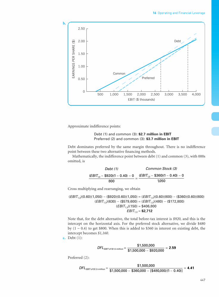
b.

Approximate indifference points:

Debt (1) and common (3): $2.7 million in EBIT

Preferred (2) and common (3): $3.7 million in EBIT

Debt dominates preferred by the same margin throughout. There is no indifferencepoint between these two alternative financing methods.

Mathematically, the indifference point between debt (1) and common (3), with 000somitted, is

Cross multiplying and rearranging, we obtain

(EBIT1,3)(0.60)(1,050) − ($920)(0.60)(1,050) = (EBIT1,3)(0.60)(800) − ($360)(0.60)(800)(EBIT1,3)(630) − ($579,600) = (EBIT1,3)(480) − ($172,800)

(EBIT1,3)(150) = $406,800EBIT1,3 = $2,712

Note that, for the debt alternative, the total before-tax interest is $920, and this is theintercept on the horizontal axis. For the preferred stock alternative, we divide $480 by (1 − 0.4) to get $800. When this is added to $360 in interest on existing debt, theintercept becomes $1,160.

c. Debt (1):

Preferred (2):

DFLEBIT of $1.5 million$1,500,000

$1,500,000=

− − −=

$ , [$ , /( . )]

360 000 480 000 1 0 404.41


$1,500,000=

−=

$ ,

920 0002.59

Debt (1)

EBIT

Common Stock (3)

EBIT( $ )( . ) ( $ )( . )

,, ,1 3 1 3920 1 0 40 0

800

360 1 0 40 0

1050− − −

=− − −


447

••

FUNO_C16.qxd 9/19/08 17:19 Page 447

Common (3):

d. For the present EBIT level, common is clearly preferable. EBIT would need to increaseby $2,712,000 − $1,500,000 = $1,212,000 before an indifference point with debt isreached. One would want to be comfortably above this indifference point before astrong case for debt should be made. The lower the probability that actual EBIT will fallbelow the indifference point, the stronger the case that can be made for debt, all otherthings the same.

4.

which reduces to

Dividing both the numerator and denominator by (P − V) produces

5. a. Total annual interest is determined as follows:

15% of $2.4 million = $ 360,00013% of $3.0 million = 390,00018% of $2.0 million = 360,000

$1,110,000

Interest coverage ratio = $2,000,000/$1,110,000 = 1.80

Total annual principal payments = $100,000 + $150,000 = $250,000

b. Required deviation of EBIT from its mean value before ratio in question becomes 1:1:

Interest coverage: $1,110,000 − $2,000,000 = −$890,000

Debt-service coverage: $1,610,000 − $2,000,000 = −$390,000

Standardizing each deviation from the mean produces the following Z-scores:

Table V in the Appendix at the end of the book can be used to determine the proportionof the area under the normal curve that is Z standard deviations left of the mean. Thisproportion corresponds to the probability that an EBIT figure will occur that producescoverage ratios lower than 1:1. For interest coverage and debt-service coverage ratiosless than 1:1, these probabilities are approximately 28 percent and 40 percent, respec-tively. These probabilities assume that the distribution of possible EBITs is normal.

c. There is a substantial probability, 40 percent, that the company will fail to cover itsinterest and principal payments. Its debt ratio (using either book or market values) ismuch higher than the industry norm of 0.47. Although the information is limited,

Debt-service coverage standard deviations (left of the mean): $ ,

$ , , .

−= −

390 0001500 000

0 260

Interest coverage 93 standard deviations (left of the mean): $ ,

$ , , .

−= −

890 0001500 000

0 5

Debt-servicecoverage ratio

$ , ,

$ , , [$ , /( . )] =

+ −=

2 000 0001110 000 250 000 1 0 50

1.24

DOLQ

Q FC P VQ

Q QQ unitsBE

=− −

=−

[ /( )]

DOLQ P V

Q P V FCQ units =−

− −

( )( )

DOL

Q P VQ P V FC

Q QQ units


output (or sales)

= =

−− −

⎡⎣⎢

⎤⎦⎥

( )( )

/

Δ

Δ


$1,500,000=

−=

$ ,

360 0001.32


448

••

FUNO_C16.qxd 9/19/08 17:19 Page 448

Donaldson, Gordon. Corporate Debt Capacity. Boston:Division of Research, Harvard Business School, 1961.

—— . “Strategy for Financial Emergencies.” HarvardBusiness Review 47 (November–December 1969), 67–79.

Gahlon, James. “Operating Leverage as a Determinant of Systematic Risk.” Journal of Business Research 9(September 1981), 297–308.

—— , and James Gentry. “On the Relationship BetweenSystematic Risk and the Degrees of Operating andFinancial Leverage.” Financial Management 11 (Summer1982), 15–23.

Harvey, Campbell R., and John R. Graham. “The Theoryand Practice of Corporate Finance: Evidence from theField.” Journal of Financial Economics 60 (May/June2001), 187–243.

Hong, Hai, and Alfred Rappaport. “Debt Capacity, OptimalCapital Structure, and Capital Budgeting.” FinancialManagement 7 (Autumn 1978), 7–11.

Levy, Haim, and Robert Brooks. “Financial Break-EvenAnalysis and the Value of the Firm.” FinancialManagement 15 (Autumn 1986), 22–26.

Myers, Stewart C. “Capital Structure Puzzle.” Journal ofFinance 39 (July 1984), 575–592.

Piper, Thomas R., and Wolf A. Weinhold. “How MuchDebt Is Right for Your Company?” Harvard BusinessReview 60 (July–August 1982), 106–114.

Zivney, Terry L. “Alternative Formulations of Degrees ofLeverage.” Journal of Financial Education 26 (Spring2000), 77–81.

Part VI of the text’s website, Wachowicz’s Web World, contains links to many finance websites and online articles related to topics covered in this chapter.(http://web.utk.edu/~jwachowi/part6.html)

based on what we have, it would appear that Archimedes has too much debt. However,other factors, such as liquidity, may mitigate this conclusion.

6. Aberez has a lower debt ratio than its industry norm. Vorlas has a higher ratio relative toits industry. Both companies exceed modestly their industry norms with respect to inter-est coverage. The lower debt-to-equity ratio and higher interest coverage for Vorlas’sindustry suggests that its industry might have more business risk than the industry ofwhich Aberez is a part. The liquidity ratio of Aberez is higher than the industry norm,whereas that for Vorlas is lower than the industry norm. Although all three financial ratiosfor Vorlas are better than are those for Aberez, they are lower relative to the industry norm.Finally, the bond rating of Aberez is much better than is that of Vorlas, being an Aa gradeand higher than the industry norm. The bond rating of Vorlas is one grade below the verylowest grade for investment-grade bonds. It is also lower than the typical company’s bondrating in the industry. If the industry norms are reasonable representations of underlyingbusiness and financial risk, we would say that Vorlas had the greater degree of risk.

Selected References


449

••

FUNO_C16.qxd 9/19/08 17:19 Page 449

operating and financial leverage - جامعة نزوى · operating leverage operating leverage is...

Documents