executive compensation and operating leverage

1

Executive Compensation and Operating Leverage

David Aboody

Anderson School of Management at UCLA

Shai Levi

Recanati Business School, Tel Aviv University

Dan Weiss

Recanati Business School, Tel Aviv University

February 2016

Abstract

We examine the effect of option-based compensation on managers’ choice of operating leverage (i.e.,

the fixed-to-variable cost ratio). First, we show a higher proportion of fixed-to-variable costs increases

earnings volatility and intensifies earnings downside potential—consequences risk-averse managers will

try to avoid. Next, we utilize the adoption of FAS 123R as an exogenous shock to managers’

compensation with no impact on the economic benefits of options. We test the effect of a reduction in

option-based compensation following the accounting change on managers’ operating-leverage choice.

Results indicate managers in firms that significantly reduce stock-option compensation subsequent to the

issuance of FAS 123R substantially reduced the level of operating leverage. Further exploring how

managers substituted fixed costs with variable costs, we find they adjusted SG&A and R&D costs but

not costs of goods sold. Consistent with the standard principle-agency model, the empirical evidence

suggests risk-taking incentives induced by option-based compensation affect cost-structure choices.

Acknowledgments: The authors are grateful for constructive suggestions and helpful comments from Yacov Amihud, Eli

Amir, Ilan Cooper, Eti Einhorn, Efrat Shust, Tzahi Versano, Alfred Wagenhofer, Avi Wohl, and participants of the seminars

at the University of Graz, Tel Aviv University and UCLA.

2

Executive Compensation and Operating Leverage

1. Introduction

Assessing the usefulness of option-based compensation in influencing managers' risk-taking

behavior has attracted much attention in the literature (Core et al., 2003). We examine the effect of

option-based compensation on managers’ choice of operating leverage. Operating leverage, defined as

the ratio of fixed to variable costs (Lev, 1974; Balakrishnan et al., 2013) is a key operative choice that

determines a firm’s cost structure. In an early study, Lev (1974) associates operating leverage and

systematic risk; that is, firms lower their risk by reducing fixed costs and increasing variable costs.

Later, Kallapur and Eldenburg (2005) build on real-options theory and report that uncertainty leads

firms to prefer technologies with low fixed and high variable costs.1 Yet, the literature has not examined

the impact of risk-taking incentives on managers’ operating-leverage choices. This study tests and finds

that (i) a higher proportion of fixed-to-variable costs increases future earnings volatility and intensifies

earnings downside potential—consequences risk-averse managers try to avoid, and (ii) a decrease in

option-based compensation leads managers to reduce operating leverage.

We show that increasing operating leverage, that is, increasing fixed costs and decreasing

variable costs, leads to higher volatility of current and future earnings. We also find that increasing

operating leverage induces an asymmetric effect on earnings. For firms with high operating leverage, the

decrease in current and future earnings when revenues fall is significantly larger than the increase in

earnings when revenues rise. Slower cost adjustment when earnings fall drives the greater earnings

downside for firms with high operating leverage. By contrast, costs are promptly adjusted when

revenues rise. Both the earnings volatility and the asymmetric effect on earnings are likely to deter risk-

averse managers from choosing high operating leverage.

1 Similarly, Novy-Marx (2010) documents operating leverage predicts cross-sectional stock returns.

3

Next, we test the effect of changes in option-based compensation on managers’ operating-

leverage choices. FAS 123R required firms to start expensing stock options, and firms decreased option-

based compensation following this change in accounting regulation (Carter et al., 2007; Brown and Lee,

2011; Hayes et al., 2012).2 The exogenous decrease in option-based compensation following FAS 123R

serves as our test setting, in line with Kallapur and Eldenburg (2005) and Hayes et al. (2012). The

reduction in option-based compensation around FAS 123R lowers managers’ risk-taking incentives.

Thus, we predict managers reduced operating leverage in response to the issuance of FAS 123R.

The results of both portfolio and regression analyses strongly support our prediction. On average,

we find managers reduced operating leverage from 12.5% before FAS 123R to 6.0% after FAS 123R.

That is, managers substituted over half of the fixed cost with variable costs. Importantly, we find a

statistically significant and economically meaningful reduction in the operating leverage only in firms

that heavily reduced option-based compensation after FAS 123R. Specifically, managers in firms with a

substantial reduction in option-based compensation after the issuance of FAS 123R lessened operating

leverage by 13.3%, whereas firms with minor or no reduction in option-based compensation display an

insignificant decrease in operating leverage. In a similar vein, we also find a reduction in pay convexity

(vega) after FAS 123R led managers to decrease operating leverage. Overall, the cutbacks in risk-taking

incentives after FAS 123R led managers to lessen the operating leverage of their firms.

To further learn how managers lowered operating leverage after FAS 123R, we examine the

change in the fixed-to-variable ratio of separate cost components. We find managers significantly

substituted fixed sales, general, and administrative (SG&A) costs and research and development (R&D)

costs with variable SG&A and R&D costs after FAS 123R, but did not change the structure of cost of

2 Guay (1999), Coles, Daniel, and Naveen (2006), and Chava and Purnanandam (2010) use simultaneous-equations methods

to examine whether risk-taking incentives have a causal effect on firm investment and financing policies. The issuance of

FAS 123R allows for using an exogenous shock for testing whether risk-taking incentives have a causal effect on operating-

leverage choices.

4

goods sold (COGS). Notably, SG&A and R&D costs became less fixed and more variable, whereas the

level (magnitude) of SG&A and R&D costs did not change after FAS 123R.

Our study makes a number of contributions to the literature. First, we show that risk-taking

incentives affect managers' cost-structure choices (i.e., the proportion of fixed-to-variable costs). The

cost-behavior literature tests numerous factors that influence managerial cost-structure choices

(Anderson et al., 2003; Banker and Byzalov, 2014), but has not yet examined the effect of compensation

schemes. We show that option-based compensation matters in making operating leverage choices.

Specifically, to the extent that the compensation change around FAS 123R is driven by the accounting

change, rather than by business circumstances, it allows us to overcome endogeneity and demonstrate

the causal effect of compensation on managers’ cost-structure choices.

Our paper also contributes to the empirical literature on the relation between compensation and

the risk-taking behavior of managers. A number of recent studies used exogenous shocks to investigate

the effect of risk-taking incentives on managerial risky choices. For instance, Gormley et al. (2013)

show that an exogenous shock to firm business risk influences risk-taking incentives, which, in turn,

affect managers’ choices of risky activities.3 By contrast, we exploit an accounting change that affected

compensation contracts, not the business risk of firms, and find the decrease in risk-taking incentives

induced by an accounting change led managers to reduce their operating leverage.

Hayes et al. (2012) use the issuance of FAS 123R test setting and find little evidence that the

decline in option-based compensation resulted in less risky choices by managers. In particular, Hayes et

al. (2012) find the change in compensation convexity (vega) did not affect the level of R&D expenses.

In line with Hayes et al., we find no significant changes in the levels of R&D or SG&A costs around

FAS 123R. We do, however, find a considerable change in the sensitivity of R&D and SG&A costs to

3 Armstrong (2013) argues the research setting of Gormley et al. (2013) is less amenable for testing the casual effect of

managers’ equity incentives on making risky choices.

5

sales changes, namely, lower operating leverage. That is, the decrease in option-based compensation

around FAS 123R caused managers to reduce the fixed-to-variable proportion, that is, the operating

leverage, but the cost levels remained unchanged. Because cost structures and their implied earnings

volatility and potential downside influence future earnings, consistent with Dichev and Tang (2009) and

Weiss (2010), the distinction between the cost level and cost structure is important for financial analysts

and for investors.

Finally, our evidence links operating leverage with the asymmetric-cost-behavior literature

(Banker and Byzalov, 2014). We document asymmetric cost behavior driven by high fixed costs.

Specifically, the results suggest high operating leverage adds an operational constraint on firm responses

to unfavorable demand shocks. That is, the results suggest cost stickiness is more pronounced for high-

operating-leverage firms than for low-operating-leverage firms, because adjusting resources is slower

for high-operating-leverage firms. Moreover, the stickiness phenomenon continues beyond the year of

the revenue shock and affects earnings in subsequent years, particularly for high-operating-leverage

firms.

The remaining sections of this paper are organized as follows: section 2 lays out the motivation

and relevant literature, section 3 describes the settings, section 4 presents the evidence on future

earnings volatility and the downside effect of high operating leverage, section 5 presents the primary

findings (options cutbacks after the issuance of FAS 123R led managers to significantly reduce the level

of operating leverage), section 6 examines how managers adjust operating leverage, and section 7

concludes.

6

2. Hypotheses and Literature Review

Before testing the impact of risk-taking incentives on managers’ choice of operating leverage, we

first demonstrate the undesirable effects of high operating leverage for risk-averse managers.

Specifically, we examine the effect of the operating leverage on earnings volatility and whether this

effect is symmetric for revenue increases and decreases.

Prior literature shows operating leverage increases firms’ risk. In an early study, Lev (1974)

shows operating leverage increases systematic risk. Novy-Marks (2010) reports operating leverage can

predict stock returns in the cross section, which links operating leverage and systematic risk (Mandelker

and Rhee, 1984). Kallapur and Eldenburg (2005) report uncertainty leads firms to prefer technologies

with low operating leverage, namely, low fixed costs and high variable costs.4 Yet, the effect of

operating leverage on future earnings has yet to be examined.

2.1 Effect of operating leverage on future earnings

Operating leverage reflects the proportion of fixed costs in a firm’s cost structure. The mix of

fixed and variable costs mediates the impact of revenue shocks on earnings, by affecting the earnings-to-

revenue slope. High operating leverage, that is, a high proportion of fixed costs to variable costs, results

in a high sensitivity of profits to changes in demand. Firms with high operating leverage tend to have

high profit margins, where a change in revenue level has a large impact on earnings (Lanen et al., 2013),

resulting in high earnings volatility. High operating leverage leads to high earnings volatility because it

conveys the impact of revenue shocks to earnings, whereas low operating leverage moderates it

(Garrison et al., 2012; Horngren et al., 2013). Although this assertion is widely accepted and taught, it

4 Both Kallapur and Eldenburg (2005) and Banker et al. (2014) investigate how demand uncertainty influences managers’

cost-structure choices. Taking a different path, this study focuses on the role of managerial risk-taking incentives in

managers’ cost-structure choices.

7

has not been empirically validated. Particularly, prior studies have not examined the relationship

between operating leverage and future earnings volatility.

Firms make long-term commitments in acquiring capacity, resulting in fixed costs. Fixed costs

arise from the possession of facilities, infrastructure, machines, and equipment and from retaining

experienced and skilled personnel. The fixed costs also include property taxes, lease payments,

depreciation, insurance, and salaries of key personnel. These fixed costs are slowly modified because of

their high cost of adjustment.

Although prior studies report an immediate cost response to revenue shocks (e.g., Chen et al.,

2012; Cannon, 2014), these studies cannot speak to whether the adjustment process is fully completed

within a concurrent year. In firms with high operating leverage, an adjustment process is likely to spread

over a long period in response to revenue shocks. Therefore, we expect high operating leverage to

influence current and future earnings volatility.

Hypothesis I: Higher operating leverage leads to greater volatility in current and future earnings.

Although the fixed-variable-cost model underlying the operating-leverage concept implies a

linear and symmetric cost structure, Anderson et al. (2003) and a large body of subsequent studies

document cost asymmetry—costs increase more when revenue rises than they decrease when revenue

falls by an equivalent amount. The reason for the asymmetric cost is asymmetric frictions in making

resource adjustments—forces acting to restrain or slow the downward adjustment process more than the

upward adjustment process (Anderson et al., 2003). Essentially, the literature explores various

immediate managerial responses to increases versus decreases in revenue, resulting in a downside effect,

and finds managers make a lower proportion of cost adjustments on the downside than on the upside.5

More importantly, making a lower proportion of cost adjustments on the downside than on the upside

5 See, e.g., Balakrishnan et al. (2004), Balakrishnan and Gruca (2008), Chen et al. (2012), Dierynck et al. (2012), Banker et

al. (2013), Kama and Weiss (2013), Cannon (2014), Holzhacker et al. (2014), Banker et al. (2014), and Shust and Weiss

(2014). Banker and Byzalov (2014) offer a review of the asymmetric-costs literature.

8

generates an earnings asymmetry—earnings increase less when revenue rises than they decrease when

revenue falls by an equivalent amount (Banker and Chen, 2006; Anderson et al., 2007; Weiss, 2010).

That is, prior studies document a concurrent downside effect—contemporaneous earnings decrease more

when revenue falls than they increase when revenue rises.

Considering the impact of operating leverage on future earnings, capacity set in advance is

expected to influence cost asymmetry (Balakrishnan et al., 2004) because the depreciation of the capital

investment remains when demand falls. Shust and Weiss (2014) report past investments enhance the

extent of cost asymmetry. That is, in firms with high operating leverage, an adjustment process is likely

to spread over a long period. Therefore, high operating leverage is likely to induce an ongoing downside

effect in response to a falling demand shock—future earnings decrease more when current revenue falls

than they increase when current revenue rises.6 However, the empirical literature has not yet looked into

the impact of operating leverage on the level of future earnings asymmetry and the longevity of the

downside effect. We expect to find that operating leverage has an enduring downside effect on future

earnings.

Hypothesis II: High operating leverage has a downside effect on future earnings: Future earnings

decrease more when revenues fall than they increase when revenues rise.

Overall, Hypothesis I asserts that high operating leverage generates volatility of earnings, and

Hypothesis II asserts that high operating leverage results in a downside effect on earnings. Both high

earnings volatility and a downside potential deter risk-averse managers from choosing high operating

leverage.

6 For example, Balakrishnan et al. (2014).

9

2.2 Effect of option-based compensation on operating leverage

Extant literature focuses on the role stock options play in providing incentives for risk taking.

For example, early studies by Amihud and Lev (1981) and Smith and Stulz (1985) note that because

managers are less diversified compared to outside shareholders, they pass up high-risk projects with

positive net present value, which would be beneficial to shareholders. Shareholders can potentially

reduce this risk-related agency problem through the use of stock options, that is, by structuring

compensation to be a convex function of firm performance. That is, stock options make the expected

wealth of managers an increasing function of performance volatility.7

Later, a number of empirical studies support the assertion that stock options encourage managers

to take risks. Guay (1999) shows higher convexity of the manager’s wealth-performance relation is

positively associated with proxies for risk taking. Sanders and Hambrick (2007) document managers

with large option holdings tend to make investments with high performance variance (big gains and big

losses).8 Armstrong and Vashishtha (2012) report that payoff convexity (vega) gives CEOs incentives to

increase their firms’ total risk by increasing systematic risk but not idiosyncratic risk.

Coles et al. (2006) attempt to establish a casual relation and find higher sensitivity of CEO

wealth to stock-price volatility leads the CEO to make more risky investments.9 However, Lewellen

(2006) reports results opposite to those of Coles et al. (2006), namely, that higher option ownership

7 Although the notion that convexity in a manager’s wealth function encourages her to take risks is appealing, analytical

studies seem to be skeptical. Lambert et al. (1991), Carpenter (2000), Hall and Murphy (2002), and Ross (2004) demonstrate

that increasing the convexity of the manager’s wealth-performance relation does not unambiguously increase the incentives

for risk taking when the manager is risk averse. Therefore, empirical evidence is important in shedding light on the validity of

this notion. 8 Smith and Swan (2008) report evidence that risk-taking incentives through stock options significantly increase the

likelihood that a firm will make risky investments. Similar evidence is provided by Rajgopal and Shevlin (2002) for gas and

oil producers, and by Mehran and Rosenberg (2007) for banks. 9 Also, Chava and Purnanandam (2010) find convexity is positively related to financial leverage. Ittner et al. (2003) argue

that under high market volatility, stock price is a noisy indicator of performance, and therefore imposes more risk on

managers.

10

tends to decrease the manager’s tendency to take risks. Apparently, the potential for endogeneity

problems made inferring causation difficult in these prior studies. Also, unobservable variables, such as

the manager’s private wealth and risk aversion, encumber the ability to control for the risk premium

associated with the manager’s compensation contract.

Recently, a number of studies used exogenous shocks to investigate how risk-taking incentives

influence managerial risky choices. Low (2009) reports firms with low convexity reduced volatility in

response to a court ruling that changed the riskiness of the business environment. Later, Gormley et al.

(2013) report managers with less convex payoffs tend to reduce risky activities.

Similar to Hayes et al. (2012), we exploit the change in the accounting treatment of stock-based

compensation under FAS 123R, which was issued by the Financial Accounting Standards Board (FASB)

in 2004 and took effect in December 2005. Specifically, we investigate the role of incentives to take

risks by using option-based compensation in setting firms' operating leverage. FAS 123R required firms

to start expensing stock options, and firms significantly decreased option-based compensation following

this change in accounting regulation (Carter et al., 2007; Brown and Lee, 2011; Hayes et al., 2012). This

exogenous decrease in option-based compensation following the issuance of FAS 123R serves as our

test setting.

The accounting change rather than shocks to the firm risk drive this change in option-based

compensation following FAS 123R (Low, 2009; Gormley et al., 2013). Therefore, it allows us to

overcome endogeneity and test the causal effect of changes in risk-taking incentives induced by changes

in compensation schemes on operating leverage. Hayes et al. (2012) use the FAS 123R setting to test the

effect of pay convexity on risky activities, and report that ―little evidence exists that the decline in option

usage following the accounting change results in less risky investment and financial policies‖ (p., 174).

In terms of costs, Hayes et al. (2012) examine the change in the levels, whereas we examine operating

11

leverage. If operating leverage and its implied earnings volatility and potential downside influence

future earnings, consistent with Dichev and Tang (2009) and Weiss (2010), the decrease in risk-taking

incentives following FAS 123R is expected to encourage managers to reduce operating leverage.

Hypothesis III: Reducing option-based compensation leads managers to adjust operating leverage

downward.

3. Sample and Setting

3.1 Sample and setting for testing Hypotheses I and II

We build on Lev (1974) for testing the impact of operating leverage on future earnings.

Estimating operating leverage, Lev (1974) runs a time-series regression of costs on revenue and uses the

estimated coefficient on revenue as a measure of a firm’s operating leverage.10

Following the same path,

Noreen and Soderstrom (1994), Banker et al. (1995), Noreen and Soderstrom (1997), Kallapur and

Eldenburg (2005), and Banker et al. (2014) use the log-linear specification for estimating time-series

regressions of costs on revenue. We build on these prior studies by estimating the following time-series

model for each firm i and year t:

OCi,k = α + βi,t REVi,k + i,k, k = t-8,…,t-1, (1)

where OC is the natural logarithm of total operating costs, estimated as revenue minus income from

operations. REV is the natural logarithm of revenue.11

As in Lev (1974), we use revenue as an imperfect proxy for the activity volume, because activity

volume levels are not observable. Employing revenue as a fundamental stochastic variable for

measuring activity levels is in line with Dechow et al. (1998), Kallapur and Eldenburg (2005), and a

number of sticky cost studies (e.g., Anderson et al., 2003; Banker and Chen, 2006; Weiss, 2010). Prior

10

Lev (1974) uses 20- and 12-year windows for estimating the time-series regressions. 11

We replicate the analyses using values of the variables rather than the natural logarithm. The results are essentially the

same.

12

studies use this specification because it is consistent with the generalized Cobb-Douglas production

function (see also Noreen and Soderstrom, 1994, and Banker et al., 1995). In estimating regression

model (1), we use windows of eight years of data per firm.

To the extent that revenue is a reasonable proxy of actual activity volume, Noreen and

Soderstrom (1994) demonstrate the coefficient β is the ratio of marginal to average costs. Because the

fixed-variable-cost model underlying the operating-leverage measurement assumes linearity, Kallapur

and Eldenburg (2005) interpret the coefficient β as the proportion of variable costs to total costs. For two

firms, i=1,2, suppose VCi is the variable costs and FCi is the fixed costs, and the estimated β1 < β2. We

get

1 - β1 > 1 - β2, (2)

1 – (VC1/(VC1+FC1)) > 1 – (VC2/(VC2+FC2), (3)

Operating Leverage of firm 1=FC1/VC1 > Operating Leverage of firm 2=FC2/VC2 . (4)

Because operating leverage is the ratio between fixed costs and variable costs, if 1 - β1 > 1 - β2, the

operating leverage of firm 1 is greater than the operating leverage of firm 2. Therefore, we utilize 1- β as

our proxy for operating leverage. Particularly, if costs are primarily fixed, then estimated 1- β is high,

indicating a high ratio of fixed-to-variable costs, which results in a high operating leverage.

Focusing on the impact of operating leverage on future profitability, our setting follows the

timeline presented in Figure 1. As mentioned above, the operating leverage is measured for the period t-

8 to t-1. Subsequently, at fiscal year t, we measure the shock to revenue, that is, whether revenue

increased or decreased in fiscal year t versus fiscal year t-1.

[Figure 1 about here]

Our sample for testing Hypotheses I and II, hereafter, the Compustat sample, includes 80,867

observations from 1962 to 2013, which encompasses all firms with data on Compustat, excluding

13

financial institutions (SIC 6000-9999) and utilities (SIC 4900-4949). In addition, we exclude firms with

total assets lower than $10 million, and firms with negative revenue or negative book value of equity.

3.2 Sample and setting for testing Hypotheses III

We exploit the change in the accounting treatment of stock-based compensation under FAS

123R, which was issued by the Financial Accounting Standards Board (FASB) on 2004 and took effect

in December 2005, to provide new evidence on the impact of changes in option-based compensation on

managerial choice of operating leverage. Our approach follows Kallapur and Eldenburg (2005), Hayes

et al. (2012), and Gormely et al. (2013). The issuance of FAS 123R eliminated the ability to expense

options at their intrinsic value, and instead required firms to begin expensing stock-based compensation

at its fair value, effectively eliminating any accounting advantages associated with stock options. The

significant reduction in stock options that followed the implementation of FAS 123R is an exogenous

shock to the managerial stock-options holdings, which offers a natural setting for testing Hypothesis III.

Our sample for testing Hypothesis III includes annual compensation information from fiscal

years 2000 through 2007. Our pre-FAS 123R period is the fiscal years 2000-2003, and the post-FAS

123R period is the fiscal years 2004-2007. As in Brown and Lee (2011), we define fiscal year 2004 as

the beginning of the post-FAS 123R period because FAS 123R was issued in 2004.12

The managerial

decisions to adjust the level of operating leverage are likely to start around the issuance of FAS 123R.

We use the ExecuComp database as our source of executive compensation data and merge it

with our main sample described above for the pre- and post-FAS 123R periods, from 2000 to 2007,

hereafter, the ExecuComp sample. We find 4,752 firm-year observations (594 firms) with relevant data

in the merged sample.

12

We replicate the analyses for a pre-FAS 123R period defined as fiscal years from 2002 to 2004 and a post-FAS 123R

period defined as fiscal years from 2005 to 2008, as in Hayes et al. (2012). The results are essentially the same.

14

To estimate the adjustment of operating leverage in response to the issuance of FAS 123R, we

follow Kallapur and Eldenburg (2005). Instead of using a long time series to estimate operating

leverage, we only use the 2000-2007 sample period and regress revenue on operating cost.

4. Tests of Hypotheses I and II

Testing Hypotheses I and II, we focus on the earnings response to revenue shocks up to three

years ahead, and use the Compustat sample for testing Hypotheses I and II. Figures reported in Table 1

show the mean (median) value of operating leverage for the Compustat sample observations, OL=1-β, is

0.076 (0.030). That is, the vast majority of the costs of the Compustat sample observations are

variable.13

Measuring earnings change over one-, two-, and three-year-ahead windows, EBITi,t+i is the

change in earnings before interest and taxes from year t to year t+i, deflated by total assets at t-1,

i=1,..,3. The sample firms exhibit an increase in their operating performance for one-, two- and three-

year-ahead windows. Specifically, the mean (median) contemporaneous change in operating income is

0.010 (0.012). Because our measure is cumulative, we expect a monotonic increase in the firms’

accounting performance. Indeed, the one-, two-, and three-year-ahead windows’ mean (median) change

in EBIT is 0.022, 0.035, and 0.051 (0.020, 0.028, and 0.037), respectively. About 28.6% of our sample

firm-years exhibit a negative demand shock, measured by a revenue decrease, RevDec. That is, 71.4%

of our sample firm-years exhibit an annual increase in revenue, consistent with prior studies (Anderson

et al., 2003).

[Table 1 about here]

13

In estimating model (1) per window of eight years, we find that 97.4% of the t-statistics in estimating are 1.96 or higher;

that is, the operating leverage is significant at the 0.05 level in 97.4% of the time-series estimations.

15

We use both portfolio analyses and regression analyses to test how negative and positive revenue

shocks affect earnings up to three years ahead. Table 2 presents our results for the portfolio analyses.14

We assign firms into three equal portfolios based on their operating leverage in year t, OLt. In addition,

all firms are independently sorted into quartiles based on their revenue growth at year t, and results are

presented for the lower quartile (revenue falls) and upper quartile (revenue rises).

Results from testing the first hypothesis are reported in Table 2. For revenue falls, the high-

operating-leverage portfolio shows a slow earnings-adjustment process starting in the concurrent year, -

4.5%, which continues through the subsequent three years (-3.4%,

-1.6%, and -0.1%, respectively). For the low-operating-leverage portfolio, we find an enduring earnings

response in the concurrent year and one year ahead (-2.3% and -0.9%, respectively), which reverses to

earnings growth in the second and third years ahead (+0.6% and +1.9%, respectively). The findings

indicate a monotonic earnings-adjustment process for high-operating-leverage firms, which continues

through the three subsequent years beyond the contemporaneous response to the revenue falls. That is,

the earnings-adjustment process when revenue falls is enduring and lasts over three years beyond the

immediate response. As reported in row A of the table, the difference between the earnings change of the

low- and high-operating-leverage firms is statistically significant in each of the four years (p-value<.01).

Overall, the results suggest high operating leverage has a negative long-lasting effect on future

profitability when revenue falls. By contrast, firms with low operating leverage have a significantly

lower decrease in profitability. Particularly, earnings decline more when revenue falls for high-

operating-leverage firms than for low-operating-leverage firms.

When revenue rises, the earnings growth of firms in the high-operating-leverage portfolio is higher

than the earnings growth of firms in the low-operating-leverage portfolio. In the high-operating-leverage

portfolio, earnings grow by 6.7% in the year of the revenue shock, year t, and by 8.3%, 9.1%, and 10.8%

14

Portfolio analysis reduces the influence of outliers, whereas regression analysis allows for control variables.

16

in years t+1, t+2, and t+3, respectively. For the low-operating-leverage portfolio, earnings increase by

5.4%, 7.4%, 8.7%, and 10.2%, in years t to t+3, respectively. As reported in row B, the difference

between the earnings growth of the low- and high-operating-leverage portfolios is statistically

significant in years t and t+1 (p-value<.01). Although the adjustment process seems shorter on the

upside, earnings increase more when revenue rises for high-operating-leverage firms than for low-

operating-leverage firms.

Overall, we conclude the earnings response to revenue shocks is greater for high-operating-

leverage firms than for low-operating-leverage firms on both the downside and the upside. That is,

operating leverage increases earnings volatility, in line with the first hypothesis.

Next, we test our second hypothesis, that operating leverage generates an earnings downside

effect. The difference between the earnings growth of high- versus low-operating-leverage portfolios is

presented in row A for revenue falls, and in row B for revenue rises. The difference between these two

effects is presented in the bottom row, marked |A|-|B|. We find the incremental impact of high operating

leverage on the change in earnings when revenue falls is significantly greater than when revenue rises in

year t, as well as in each of the three subsequent years (p-value<.01 in each of the four years). For

instance, the incremental impact of high operating leverage over low operating leverage in the first

subsequent year, t+1, is +1.6% (p-value<0.01).15

That is, we observe the difference in performance for

the high-operating-leverage group relative to the low-operating-leverage group (see bottom row) is

greater for the negative revenue shocks (see row A) than for the positive revenue shocks (see row B).

The evidence indicates a substantial enduring downside effect for firms with high operating leverage:

15

We also observe that in the low-operating-leverage portfolio of Table 2, 32.76% of observations have a revenue decrease,

whereas in the high-operating-leverage portfolio, 27.71% of observations have a revenue decrease. The Wilcoxon test for the

difference between the two proportions is 12.77 (p-value <.0001). Hence, the high-operating-leverage portfolio experiences

significantly more positive revenue shocks than the low-operating-leverage portfolio.

17

future earnings decrease significantly more when revenues fall than they increase when revenues rise.

This downside effect is in line with the second hypothesis.


To further test our two hypotheses, we estimate the following regression model:

ΔEBITi,t+k = α + β1 OLi,t + β2 RevDeci,t + β3 RevDeci,t OLi,t + β4 ΔEBITi,t-1 + β5 MVi,t-1

+ β6 BMi,t-1+εi,t, k= 0,1,2,3. (5)

We estimate model (5) separately for changes in EBIT over each of four horizons, from year t to

year t+k, where k= 0,1, 2, 3. Thus, ΔEBITi,t+k is the accumulated change in earnings before interest and

taxes from year t to year t+k, where k goes from 0 to 3, deflated by total assets at t-1. RevDeci,t is an

indicator variable that equals 1 if revenue in year t was lower than revenue in year t-1. OLi,t is operating

leverage defined as 1-βi,t, where βi,t is defined by model (1). ΔEBITi,t-1 is the change in earnings before

interest and taxes from year t-2 to year t-1, deflated by total assets at t-2. MV i, t-1 is the natural log of

the market value of the firm at the end of year t-1. B/M i, t-1 is the book value of equity divided by the

market value of equity at the end of year t-1. In addition, we include both year and industry fixed

effects, using Fama and French’s (1997) 12-industry classification. Finally, all significance levels are

based on standard errors that are clustered by firm and year.

The coefficients β1 and β3 are the focus of our tests. The association between operating leverage

and future earnings when revenue rises is captured by β1. The interactive term of operating leverage

multiplied by revenue fall, or more specifically, the coefficients β1+β3, capture the association between

operating leverage and future earnings when revenue falls. Significant positive values for β1 and

significant negative values for β1+β3 support our first hypothesis, indicating a significant long-lasting

association between operating leverage and future earnings volatility, consistent with Hypothesis I. A

significant negative estimate for coefficient β3 supports Hypothesis II.

18

Our control variables are as follows: the change in EBIT from year t-2 to year t-1, ΔEBITi, t-1,

controls for the time-series properties of earnings that can affect future earnings. Market value, MVi, t-1,

and the book-to-market ratio, BMi, t-1, control for potential effects of risk and growth (Fama and French,

1992).

Estimation results are reported in Panel A of Table 3. For a positive revenue shock, the

contemporaneous (k=0) β1 is positive and significant (β1=0.028, t-statistic=9.17). The coefficient β1 is

also significant and positive for one year ahead (β1=0.022, t-statistic=3.76), and marginally significant

for two years ahead (β1=0.016, t-statistic=1.75). However, β1 is insignificant for three years ahead

(β2=0.014, t-statistic=1.28). Thus, when revenue rises, operating leverage significantly affects

profitability growth two years ahead, and by the third year, the effect of operating leverage on

profitability fades. For the concurrent year and two years ahead, earnings increase more when revenue

rises for high-operating-leverage firms than for low-operating-leverage firms, consistent with

Hypothesis I.

When revenue falls, β1+β3 is significant and negative in year t (β1+β3=0.028-0.074=

-0.046, t-statistic= -7.82). Looking ahead, β1+β3 is significant and negative one year after the revenue

shock, at year t+1 (β1+β3 =0.022-0.067=-0.045, t-statistic= -4.22), two years ahead (β1+β3 = 0.016-

0.060=-0.044, t-statistic= -3.20), and three years ahead (β1+β3 =0.014-0.055=-0.041, t-statistic= -3.04).

So when revenue falls, operating leverage has a long-lasting effect on profitability, of at least three

years. Notably, up to three years ahead, earnings decline more when revenue falls for high-operating-

leverage firms than for low-operating-leverage firms, consistent with Hypothesis I.

The second hypothesis predicts a downside effect for high-operating-leverage firms: future

earnings decrease more when revenues fall than they increase when revenues rise. As reported in Panel

A of Table 3, β3 is significant and negative in year t of the revenue shock, year t (β3=-0.074, t-statistic=-

19

12.15), β3 is significant and negative for earnings one year ahead, year t+1 (β3= -0.067, t-statistic=-6.60),

for two years ahead (β3 = -0.060, t-statistic=-4.92), and for three years ahead (β3 =

-0.055, t-statistic=-5.21). That is, in the year of the revenue shock as well as in each of the three

subsequent years, β3 is negative and significant, in line with Hypothesis II.

In other words, the results suggest operating leverage enhances a downside profitability effect.

The evidence indicates a substantial enduring downside effect for firms with high operating leverage:

future earnings decrease significantly more when revenues fall than they increase when revenues rise.

This downside effect supports the second hypothesis.

As for the control variables, ΔEBITi,t-1 is negative and significant, capturing the mean reversion

in operating performance. Similarly, both market value and market-to-book value are negative,

indicating larger and more mature firms have less volatility in their operating performance.

We also take a direct approach to gain further confidence in our findings. Specifically, we

compute a firm-specific standard deviation of earnings and revenues on the four-year period from year t

to t+3: (EBITit,..,t+3) = (EBITi,t, EBITi,t+1, EBITi,t+2, EBITi,t+3) and (REVit,..,t+3) = (REVi,t, REVi,t+1,

EBITi,t+2, REVi,t+3). We estimate the following regression model with the following specification:

(EBITit,..,t+3) = α + β1 OLi,t + β2 (REVit,..,t+3) + β3 (REVit,..,t+3) OLi,t + β4 MVi,t-1

+ β5 BMi,t-1 + εi,t. (6)

The estimation results are presented in column (5) of Table 3. Consistent with Hypothesis I, we

find operation leverage increases the volatility of future earnings. Both the coefficients on OLit and on

(REVit,..,t+3) OLi,t are positive, 0.038 and 0.180, respectively, and significant at the 0.01 level. Again,

results from estimating model (6) suggest operating leverage increases the volatility of future earnings,

consistent with the first hypothesis.

In sum, the results from both the portfolio and regression analyses support both Hypotheses I and

II. We find that (i) greater operating leverage results in greater earnings volatility up to three years

20

ahead, and (ii) high operating leverage has a downside effect on future earnings: Future earnings

decrease more when revenues fall than they increase when revenues rise.


4.1 Sensitivity Analyses

4.1.1 Cost-adjustment processes

We confirm the impact of operating leverage on future earnings by examining whether cost-

adjustment processes drive the phenomena at hand. We estimate the following specification16

:

ΔEXPi,t+k = α + β1 OLi,t + β2 RevDeci,t + β3 RevDeci,t OLi,t + β4 ΔEBITi,t-1 + β5 MVi,t-1

+ β6 BMi,t-1 + εi,t, k= 0,1,2,3. (7)

where EXPt+i = (EXPt+i- EXPt)/Assetst-1, i=1,..,3, is the change in operating expenses in year t+i

relative to year t, deflated by lagged total assets, and operating expenses are revenue minus earnings

before interest and taxes. As before, we include both year and industry fixed effects, using Fama and

French’s (1997) 12-industry classification, and all significance levels are based on standard errors that

are clustered by firm and year.

Results are reported in Table 4. The coefficient β1 is negative and significant for k=0 and for

k=1, and insignificant for k=2 and for k=3. As before, when revenue rises, operating leverage

negatively affects the level of expenses for two years (because variable costs are low), and by the third

year, the effect of operating leverage on the level of costs disappears. That is, for k=0 and k=1, expenses

increase less when revenue rises for high-operating-leverage firms than for low-operating-leverage

16

We also estimate a more complex specification using a continuous revenue variable. All the findings are essentially the

same. This analysis confirms the use of a dummy revenue-shock variable is not crucial for our results. Also, revenue shocks

may be correlated (Fairfield et al., 2009). Addressing this potential correlation, we control for future revenue changes. Again,

our findings support the hypotheses and our conclusions hold. See also our analysis of two consecutive revenue shocks.

21

firms. Accordingly, earnings increase more when revenue rises for high-operating-leverage firms than

for low-operating-leverage firms, consistent with Hypothesis I.

When revenue falls, β1+β3 is significant and positive in year t (β1+β3=-0.025+0.127=

+0.102, t-statistic= 10.00). β1+β3 is significant and negative one year after the revenue shock, at year t+1

(β1+β3 =-0.037+0.175=+0.138, t-statistic= 6.44), two years ahead (β1+β3 =

-0.038+0.185=+0.147, t-statistic= 4.41), and three years ahead (β1+β3 =

-0.035+0.151=0.116, t-statistic= 2.39). Namely, expenses decline less when revenue falls for high-

operating-leverage firms than for low-operating-leverage firms. Therefore, earnings decline more when

revenue falls for high-operating-leverage firms than for low-operating-leverage firms, in line with

Hypothesis I. Keeping in mind that operating leverage is the ratio of fixed costs to variable costs, the

findings suggest the cost-adjustment process is both smaller and slower for high-operating-leverage

firms. We conclude that slow cost-adjustment processes, particularly on the downside, drive the

phenomena at hand, as predicted by Hypotheses I and II.


4.1.2 Two consecutive revenue shocks

We examine future earnings in periods following two consecutive increases or decreases in

revenue (rather than a single revenue shock examined earlier). If high operating leverage induces future

earnings volatility and the downside effect, we expect a consistent cost-adjustment process, which is

likely to start after the first demand shock and continue up to three years ahead. Therefore, we sort the

sample firms into two portfolios based on their revenue growth. Two consecutive revenue decreases are

firms with revenue decreases in both years t and t+1. Two consecutive revenue increases are firms with

revenue increases in both years t and t+1. In each of the two portfolios, we also sort firms into three

portfolios based on operating leverage at time t.

22

Results reported in Table 5 for two consecutive revenue decreases indicate a monotonic relationship

between the operating-leverage portfolio and firm performance in the contemporaneous and one-, two-,

and three-year-ahead portfolios. That is, we report earnings growth on three years following two

consecutive revenue changes. Particularly, earnings decline significantly more for high-operating-

leverage firms than for low-operating-leverage firms in the contemporaneous and one-, two-, and three-

year-ahead portfolios. For two negative consecutive revenue shocks, the findings reconfirm the earlier

results for the single revenue shock reported in Tables 2 and 3. By contrast, for two consecutive revenue

increases, earnings increase significantly more for high-operating-leverage firms than for low-operating-

leverage firms in the contemporaneous and one-, two-, and three-year-ahead portfolios. For two positive

consecutive revenue shocks, the findings indicate a long-lasting effect over three subsequent years,

resulting in significant earnings volatility, in line with Hypothesis I.

Testing the second hypothesis, the under-performance of firms with high operating leverage over

firms with low operating leverage on the downside significantly exceeds the over-performance of firms

with high operating leverage over firms with low operating leverage on the upside (see results reported

in the bottom row in Table 5). That is, the results show a clear earnings-downside effect when revenues

fall in two consecutive periods.


4.1.3 ExecuComp sample

We replicate the analyses using the ExecuComp sample. The results (untabulated) are essentially

the same, but the statistical significance is weaker because of the smaller sample size. Taken as a whole,

the empirical evidence supports both Hypotheses I and II.

5. Tests of Hypothesis III

23

In this section, we test the third hypothesis, namely, whether a decrease in option-based

compensation led managers to adjust operating leverage downward. If the relation between risk-taking

incentives generated by option-based compensation and the adjustment of operating leverage is causal,

we should observe lower operating leverage as firms shift away from option-based compensation in

response to FAS 123R.

To estimate the adjustment of operating leverage in response to the issuance of FAS 123R, we

follow Kallapur and Eldenburg (2005), who tested whether managers modified the fixed-to-variable cost

ratio in response to a new Medicare reimbursement scheme. They use time-series specification to

estimate the firm-specific change in the fixed-to-variable cost ratio in response to an exogenous shock.

Following the same firm-specific approach, we test whether firms responded to a reduction in option-

based compensation by changing the fixed-to-variable cost ratio. Similar to Kallapur and Eldenburg

(2005), we estimate the following model for each firm:

, (8)

where OC is the natural logarithm of total operating costs, which are adjusted to recognize compensation

expense before FAS 123R. The fair value of options granted were expensed only following FAS 123R.

To make operating expenses before and after FAS 123R comparable, we add the fair value of options to

the operating expenses before 123R. This adjustment is similar, for example, to Barth et al. (2012). REV

is the natural logarithm of revenue, and D123R

is a dummy variable that equals 0 for years 2000-2003,

and 1 for 2004-2007. The operating leverage in the pre-FAS 123R is estimated by 1- β1 and the

operating leverage in the post-FAS 123R is estimated by

1-β1-β3. Accordingly, the coefficient β3 on the interaction REV*D123R

captures the change in operating

leverage around the issuance of FAS 123R.

24

Next, we compute the change in the value of the options portfolio in the post-FAS 123R period

relative to the pre-FAS 123R period. The value of the options portfolio is the year-end Black-Scholes

value of the executive’s options portfolio, which includes current-year grants, previously granted

unvested options, and vested options. We use ExecuComp data to calculate the value of the options

portfolio following, for example, Coles et al. (2013). Change in the value of the options portfolio of the

top five executives is calculated as the change in the value of the options portfolio of each of the top five

executives from 2000-2003 to 2004-2007, that is, the mean value of the options portfolio in 2004-2007

minus its mean value in 2000-2003.

Results reported in Table 6 show a mean decline of -8.2% (p-value<0.01) in the proportion of the

options value in the outstanding portfolios of shares and options held top five executives. Also, we find

a mean decline of -10.6% (p-value<0.01) in the proportion of the value of options granted to the top five

executives. This decline is consistent with previously reported declines in the proportion of option-based

compensation after the issuance of FAS 123R (Carter et al., 2007; Brown and Lee, 2011; Hayes et al.,

2012).17

We also classify the sample firms into two groups—below-median and above-median change in

the value of options of the top five executives from the pre-FAS 123R period, 2000-2003, to the post-

FAS 123R period, 2004-2007. Table 6 presents the mean change in the value of options for the two

groups. Specifically, the decline in the proportion of the options value in the below-median-change

group is -11.3% (p-value<0.01), whereas the respective decline in the above-median-change group is -

5.2% (p-value<0.01). That is, the decrease in the mean option value in the below-median-change group

is more than twice as great as the respective decrease in the above-median-change group. We observe

the change in option-based compensation following FAS 123R varies considerably across firms.


17

As in prior studies, we observe an increase in restricted stock compensation around FAS 123R.

25

In line with Hayes et al. (2012), reducing managers’ option-based compensation following the

issuance of FAS 123R allows us a natural setting for testing the impact of an exogenous reduction in

option-based compensation on managers’ decision to adjust operating leverage. Building on a time-

series specification for estimating firm-specific changes in operating leverage (as in Kallapur and

Eldenburg, 2005), we compare changes in operating leverage around FAS 123R between firms with

below-median and above-median change in the value of options of the top five executives around FAS

123R. Specifically, we utilize the classification of the sample firms into below-median and above-

median change in the value of options around FAS 123R. Testing Hypothesis III, we test the relation

between the change in options value around FAS 123R and the adjustment of operating leverage around

FAS 123R separately in the below-median-change group versus the above-median-change group.

Hypothesis III predicts greater downward adjustments in the below-median-change group of firms than

in the above-median-change group of firms. We also examine the robustness of our findings to replacing

the change in the value of options as our incentive measure with pay-performance convexity (vega) and

pay-performance sensitivity (delta).

Our approach allows us to estimate the mean firm-specific adjustment of operating leverage in

the post-FAS 123R period for firms with below-median versus above-median change in the value of

options around FAS 123R. Our approach follows Hayes et al. (2012) in utilizing the within-firm

difference in the value of options around FAS 123R. However, we use time-series data to estimate the

firm-specific adjustment of operating leverage in response to FAS 123R, in contrast with the panel

estimation in Hayes et al. (2012). Although panel estimation is usually more efficient, it may inflate the

significance of the results if appropriate measures are not used to control for cross-sectional and firm-

specific variation (Greene, 2011). Our approach is appropriate because the operating-leverage literature

does not offer adequate controls.

26

Results from testing Hypothesis III are reported in Table 7.18

On average, we find operating

leverage declined from 13% = 1 – 87% before FAS 123R to 7.6% = 1 – 87% – 5.4%, where the

difference is statistically significant (p-value < 0.01). On average, the level of operating leverage was

adjusted downward after the issuance of FAS 123R to less than half its value before the issuance of FAS

123R. Notably, the operating leverage was adjusted downward after the issuance of FAS 123R by 12.0%

in the below-median-change group, that is, firms with a substantial decline in option-based

compensation after the issuance of FAS 123R. On the other hand, the adjustment of operating leverage

was insignificant for firms in the above-median-change group.

Overall, the findings suggest that, on average, the exogenous reduction in option-based

compensation following FAS 123R encouraged managers to adjust operating leverage downward.

Particularly, the operating-leverage-downward adjustment is significant and economically meaningful in

firms with a considerable reduction in option-based compensations. We conclude that a reduction in

managers’ option-based compensation led them to adjust operating leverage downward, in support of

Hypothesis III.


5.1 Sensitivity analyses

5.1.1 CEOs

Although the decision to lessen operating leverage is likely to be taken by all firm executives, in

some firms the CEO may be highly influential. Therefore, we test Hypothesis III with respect to the

value of options of CEOs, rather than the top five executives of firms. Results reported in Table 8

indicate that for the below-median-change group of firms, the operating leverage was adjusted

18 Using ExecuComp data from 1992 through 2013 for testing Hypothesis III, we confirm the operating leverage of the

ExecuComp sample and the Compustat sample are compatible. The mean (median) value of operating leverage, OL=1-β,

estimated using model 1 and ExecuComp sample observations, is 0.078 (0.034), which is insignificantly different from the

respective values estimated earlier for the Compustat sample (see Table 1).

27

downward after the issuance of FAS 123R by 11.0%, whereas the adjustment of operating leverage is

insignificant for the above-median-change group of firms. The results reconfirm the earlier findings.


5.1.2 Vega and delta

We check the sensitivity of the findings to using payoff convexity (vega) and pay-performance

sensitivity (delta) as proxies for changes in compensation incentives (as in Hayes et al. 2012). Vega is

the change in the value of the top five executives’ total portfolio of current and outstanding prior grants

of shares and options for a 1% change in stock-price volatility. Delta is measured as the change in the

value of the top five executives’ total portfolio of current and outstanding prior grants of shares and

options for a 1% change in the stock price. We calculated vega and delta following Core and Guay

(2002) and Coles et al. (2006). See details in Coles et al. (2013). The change in vega (or delta) is the

percent change in vega (or delta) from the mean value in 2000-2003 to the mean value in 2004-2007.

We take the within-firm difference of each variable (vega, delta) and use it for classifying two groups of

firms (below-median and above-median changes in vega/delta around FAS 123R). As earlier, we

estimate model 8 for each firm and report the mean coefficients.

Results reported in Panel A of Table 9 indicate operating level was significantly adjusted

downward by 8.9% in the group of below-median change in vega, that is, in the group of firms with a

considerable decline in payoff convexity. By contrast, the adjustment of operating leverage in the group

of above-median change in vega, that is, in the group of firms with a minor or no decline in payoff

convexity, was 1.8% and insignificant. We conclude a large decrease in payoff convexity led managers

to adjust operating leverage downward. To the extent that vega captures managers’ aversion to earnings

28

volatility and a potential downward effect,19

the results further corroborate the earlier findings and

support Hypothesis III.

Although our findings are consistent with Gormley et al. (2013), Hayes et al. (2012) utilize vega

as a basis for finding weak evidence that the decline in option usage following FAS 123R results in less

risky investment and financial policies (changes in R&D, changes in capital expenditures, changes in

financial leverage, changes in cash holdings, changes in stock volatility). By contrast, we find a

significant relation between the decline in option usage following FAS 123R and the adjustment of

operating leverage. The difference stems from the following reasons: (i) to the extent that operating

leverage was optimal in the pre-FAS 123R, reducing option-based compensation encourages risk-averse

managers to adjust operating leverage downward to achieve lower earnings volatility and avoid a

potential downside earnings effect, (ii) managers are likely to prefer substituting fixed costs with

variable costs to cutting the total level of costs (see also empirical evidence in the next section), and (iii)

the findings are driven by firms with large decreases in option-based compensation around FAS 123R,

whereas the phenomena marginally exists in firms with small or no decreases in option-based

compensation around FAS 123R.

To complete the picture, we also test the relation between changes in pay-performance sensitivity

(delta) and changes in operating leverage. We keep in mind that the results may reflect two potential

opposite effects of delta on risk taking: a higher delta more closely aligns the manager’s incentives to

increase stock price with those of shareholders, but an increase in delta exposes the manager to

additional risk. Therefore, the pay-performance sensitivity (delta) does not lend itself to testing

Hypothesis III. Results reported in Panel B of Table 9 indicate operating leverage was adjusted

downward by 14.2% in the below-median change in the delta group of firms, whereas the adjustment of

19

Guay (1999), Coles et al. (2006), and Chava and Purnanandam (2010) report managers with greater convexity in their

compensation (i.e., vega) make riskier investment and financing choices.

29

operating leverage was insignificant in the above-median change in the delta group of firms. The

direction of these findings is generally consistent with the direction of the findings in Hayes et al.

(2012).


Taken as a whole, the evidence suggests reducing option-based compensation leads managers to

adjust operating leverage downward, particularly in firms with a substantial decline in option-based

compensation. The empirical evidence supports Hypothesis III.

6. How did managers adjust operating leverage?

To complete the picture, we provide insight into how managers adjust operating leverage. This

information is meaningful not only because it would further corroborate our primary conclusion—

reducing option-based compensation leads managers to adjust operating leverage downward—but also

because it would expand our understanding of how managers shape their firms’ cost structures.

For instance, outsourcing business activities is likely to change a firm’s cost structure because of

the need to maintain less infrastructure and because lower capacity results in lower fixed costs as well as

increasing variable costs that are sensitive to outputs and revenues (Lavina and Ross, 2003). That is,

outsourcing substitutes fixed costs with variable costs, namely, lower operating leverage.

Demonstrating this point, IBM substantially expanded its outsourcing of services in the post-

FAS 123R period.20

In the post-FAS 123R period, IBM substituted fixed costs of maintaining service

capacity in the United States with variable costs of purchasing these services from contractors in India

and China. Computing the change in the operating leverage of IBM, we find it decreased from

OL=0.238 in the pre-FAS 123R period to OL=0.090 in the post-FAS 123R period, a drop of about 60%.

20

See IBM third-quarter-earnings announcement reported on October 16, 2007, and ―IBM and the Rebirth of Outsourcing‖

by Douglas McIntyre, Time Magazine, March 26, 2009.

30

Empirically addressing this issue, we look into the cost components managers change when they

adjust operating leverage. Specifically, we examine changes in the cost of goods sold, COGS, in sales,

general, and administrative expenses, SG&A, and in research and development costs, R&D. COGS and

SG&A are the core cost components that are expected to respond to revenue shocks. We estimate a

model similar to model (8) with separate cost components as the dependent variable:

(9)

Results reported in Panel A of Table 10 display the results from estimating model 9 for COGS.

Interestingly, for firms in either below-median- or above-median-change groups, the mean coefficient on

REV*D123R

is insignificant, suggesting the change in operating leverage in the post-FAS 123R is

insignificant for both groups. We conclude that COGS was not the vehicle managers used to adjust

operating leverage. Notably, in the pre-FAS 123R, the operating leverage was 7.2% = 1-0.928 for the

below-median-change group and 2.4% = 1-0.976 for the above-median-change group. That is, the

operating leverage was low before the issuance of FAS 123R, which left little room for reducing it. This

result is consistent with Weiss (2010), who reports COGS linearly respond to changes in revenue, which

indicates COGS are primarily variable costs.

Results reported in Panel B from estimating model 9 for SG&A costs indicate that for firms in

the below-median-change group, managers adjusted operating leverage downward by 16.3% (p-

value<0.01). By contrast, for firms in the above-median-change group, the mean operating-leverage

adjustment was insignificant. That is, firms in the below-median-change group substituted fixed SG&A

costs with variable SG&A costs in the post-FAS 123R period. These results are consistent with Banker

et al. (2011), who showed how long-term incentives influence SG&A expenses, and with Janakiraman

(2010). We conclude SG&A costs served as the vehicle for substituting fixed SG&A costs with variable

SG&A costs in the post-FAS 123R period. The findings suggest managers can exercise discretion with

31

respect to resources consumed for marketing and advertising, distribution, and information technology,

which provides room for managerial decision to substitute fixed SG&A costs with variable SG&A costs.

Results from estimating model 9 using R&D costs are reported in Panel C. The evidence

indicates managers in firms in the below-median-change group significantly adjusted operating leverage

downward by 31.4% (p-value<0.01). That is, managers in the below-median-change group heavily

substituted fixed R&D costs with variable R&D costs. As for SG&A costs, the results suggest R&D

costs served as the vehicle for adjusting the level of operating leverage downward in the post-FAS 123R

period. This result is consistent with prior studies arguing managers set their R&D costs in proportion to

revenues (Hambrick et al., 1983).

Notably, the mean change around FAS 123R in the level of SG&A/Total assets was insignificant

(0.12%, t-value=0.23) for firms in the below-median-change group, and marginally significant (0.67%,

t-value =1.77) for firms in the above-median-change group. Similarly, the mean change in the level of

R&D/Total assets around FAS 123R was insignificant (0.02%, t-value=0.23) in the below-median-

change group, and also insignificant (-0.15%, t-value =-1.02) for firms in the above-median-change

group. The findings indicate managers substituted fixed SG&A (R&D) costs with variable SG&A

(R&D) costs, that is, reduced operating leverage, but the magnitude (level) of both SG&A and R&D

costs remained unchanged. This result suggests operating leverage matters in understanding managers’

choices in response to changes in risk-taking incentives.

Taken as a whole, the findings suggest managers adjusted operating leverage downward in the

post-FAS 123R period by substituting fixed SG&A and R&D costs with the respective variable costs.

Notably, we find managers chose to adjust the fixed-to-variable ratio of SG&A and R&D costs, but the

fixed-to-variable ratio of COGS remained unchanged.21

21

Hayes et al. (2012) report that, on average, firms reduced capital expenditures after the issuance of FAS 123R. Estimating

model 9 using depreciation as a cost component, we find that, on average, change in the fixed-to-variable ratio was

32


7. Summary

We examine the effect of option-based compensation on managers’ choice of operating leverage,

namely, the fixed-to-variable cost ratio. We have two main empirical findings. First, we show higher

operating leverage leads to an increase in future earnings volatility and intensifies earnings downside

potential—consequences risk-averse managers try to avoid. Second, we show option-based

compensation affects managers’ choice of operating leverage. Specifically, we use the decrease in

option-based compensation following the issuance of FAS 123R to overcome the endogeneity and test

the effect of changes in option-based compensation on operating leverage. We find the reduction in

option-based compensation led managers to lower operating leverage, and specifically to use more

variable sales, general, and administrative costs following FAS 123R. Our study demonstrates risk-

taking incentives affect managers’ choice of operating leverage.

marginally significantly in the post-FAS 123R period. We note that a change in the level of capital expenditures and a change

in the fixed-to-variable ratio of depreciation are not comparable.

33

References

Amihud, Y., Lev, B. 1981. Risk reduction as a managerial motive for conglomerate mergers. The Bell

Journal of Economics 12(2), 605–617.

Anderson, M., Banker, R., Huang, R., Janakiraman, S. 2007. Cost behavior and fundamental analysis of

SG&A costs. Journal of Accounting Auditing and Finance 22 (1), 1–28.

Anderson, M., Banker, R., Janakiraman, S. 2003. Are selling, general and administrative costs ―sticky?‖

Journal of Accounting Research 41, 47–63.

Armstrong, C.S. 2013. Discussion of ―CEO compensation and corporate risk-taking: Evidence from a

natural experiment.‖ Journal of Accounting and Economics 56, 102–111.

Armstrong, C.S.,Vashishtha, R., 2012. Executive stock options, differential risk-taking incentives, and

firm value. Journal of Financial Economics 104, 70–88.

Balakrishnan, R., Gruca, T. S. 2008. Cost stickiness and core competency: A note.

Contemporary Accounting Research 25 (4), 993–1006.

Balakrishnan, R., Labro, E., Soderstrom, N. S. 2014. Cost structure and sticky costs. Journal of

Management Accounting Research. 26(2), 91–116.

Balakrishnan, R., Petersen, M., Soderstrom, N. S. 2004. Does capacity utilization affect the ―stickiness‖

of cost? Journal of Accounting Audit and Finance. 19, 283–299.

Balakrishnan, R., Sivaramakrishnan, K., Sprinkle, G., 2013. Managerial Accounting. Wiley, New York.

Banker, R. D., Byzalov, D., Ciftci, M., Mashruwala, M. 2013. The moderating effect of prior revenues

changes on asymmetric cost behavior. Journal of Management Accounting Research. 26(2), 221-242.

Banker, R. D., Byzalov, D. 2014. Asymmetric cost behavior. Journal of Management Accounting

Research 26(2), 43-79.

Banker, R. D., Byzalov, D., Chen, L. 2013. Employment protection legislation, adjustment costs and

cross-country differences in cost behavior. Journal of Accounting and Economics 55(1), 111–127.

Banker, R.D., Byzalov, D., Plehn-Dujowich, J. 2014. Sticky cost behavior: Theory and evidence. The

Accounting Review 89(3), 839–865.

Banker, R.D., Chen, L. 2006. Predicting earnings using a model of cost variability and cost stickiness.

The Accounting Review 78, 285–307.

34

Banker, R. D., Huang, R., Natarajan, R. 2011. Equity incentives and long-term value created by SG&A

expenditure. Contemporary Accounting Research 28(3), 794–830.

Banker, R. D., Potter, G., Schroeder, R. G. 1995. An empirical analysis of manufacturing overhead cost

drivers. Journal of Accounting and Economics 19, 115–37.

Barth, M. E., Gow, I. D., Taylor, D. J. 2012. Why do pro forma and Street earnings not reflect changes

in GAAP? Evidence from SFAS 123R. Review of Accounting Studies 17(3), 526–562.

Brown, L. D., Lee, Y. J. 2011. Changes in option-based compensation around the issuance of SFAS

123R. Journal of Business Finance & Accounting 38(9-10), 1053–1095.

Cannon, J. N. 2014. Determinants of "sticky costs": An analysis of cost behavior using United States air

transportation industry data. The Accounting Review. 89(5), 1645–1672.

Carpenter, J., 2000. Does option compensation increase managerial risk appetite? Journal of Finance 55,

2311–2331.

Carter, M. E, Lynch, L. J., Tuna, I. 2007. The role of accounting in the design of ceo equity

compensation. The Accounting Review 82(2), 327–357.

Chava, S., Purnanandam, A., 2010. CEOs vs. CFOs: incentives and corporate policies. Journal of

Financial Economics 97, 263–278.

Chen, C. X., Lu, H., Sougiannis, T. 2012. The agency problem, corporate governance, and the

asymmetrical behavior of selling, general, and administrative costs. Contemporary Accounting

Research 29, 252–282.

Coles, J., Daniel, N., Naveen, L., 2006. Managerial incentives and risk taking. Journal of Financial

Economics 79, 431–468.

Coles, J., Daniel, N., Naveen, L., 2013. Calculation of compensation incentives and firm-related wealth

using Execucomp: Data, Program, and Explanation, working paper.

Core, J., Guay, W., 2002. Estimating the value of employee stock option portfolios and their sensitivities

to price and volatility. Journal of Accounting Research 40, 613–630.

Core, J. E., Guay, W. R., Larcker, D. F. 2003. Executive equity compensation and incentives: A

survey. Economic Policy Review, 9(1).

Dechow, P., Kothari, S., Watts, R. 1998. The relation between earnings and cash flows. Journal of

Accounting and Economics 25, 133–168.

Dichev, I. V., Tang V. W., 2009. Earnings volatility and earnings predictability. Journal of Accounting

and Economics 47, 160–181

http://www.sciencedirect.com/science/journal/01654101

http://www.sciencedirect.com/science/journal/01654101

http://www.sciencedirect.com/science/journal/01654101/47/1

35

Dierynck, B., Landsman, W., Renders, A. 2012. Do managerial incentives drive cost behavior?

Evidence about the role of the zero earnings benchmark for labor cost behavior in Belgian private

firms. The Accounting Review 87(4), 1219–1246.

Fairfield, P. M., Ramnath, S., Yohn, T. L. 2009. Do industry-level analyses improve forecasts of

financial performance? Journal of Accounting Research 47(1), 147–178.

Fama, E. F., French, K. R. 1992. The cross-section of expected stock returns. The Journal of Finance

47, 427–465.

Fama, E. F., French, K. R., 1997. Industry costs of equity. Journal of Financial Economics 43, 153–193.

Garrison, R. H., Noreen, E. W., Brewer, P. C. 2012. Managerial Accounting, 14th

ed. McGraw Hill,

New York.

Gormley, T. A., Matsa, D.A., Milbourn, T., 2013. CEO compensation and corporate risk: Evidence from

a natural experiment. Journal of Accounting and Economics 56, 79–101.

Greene, W.H. 2011. Econometric Analysis, Seventh edition.

Guay, W., 1999. The sensitivity of CEO wealth to equity risk: an analysis of the magnitude and

determinants. Journal of Financial Economics 53, 43–71.

Hall, B., Murphy, K., 2002. Stock options for undiversified executives. Journal of Accounting and


Hambrick, D. C., MacMillan, I. C., Barbosa, R. R. 1983. Business unit strategy and changes in the

product r&d budget. Management Science 29(7), 757–769.

Hayes, R.M., Lemmon, M., Qiu, M. 2012. Stock options and managerial incentives for risk taking:

Evidence from FAS 123R. Journal of Financial Economics 105, 174–190.

Holzhacker, M., Krishnan, R., Mahlendorf, M. 2014. The impact of changes in regulation on cost

behavior. Contemporary Accounting Research. Forthcoming.

Horngren, C. T., Sundem, G. L., Schwartzberg, J. O., Burgstahler, D. 2013. Introduction to Management

Accounting, 16th

ed. Pearson, Upper Saddle River, NJ.

Ittner, C., Lambert, R., Larcker, D., 2003. The structure and performance consequences of equity grants

to employees of new economy firms. Journal of Accounting and Economics 34, 89–127.

Kallapur, S., Eldenburg, L. 2005. Uncertainty, real options, and cost behavior: Evidence from

Washington State hospitals. Journal of Accounting Research 43 (5), 735–752.

Kama, I., Weiss, D. 2013. Do earnings targets and managerial incentives affect sticky costs? Journal of

Accounting Research 51 (1), 201–224.

36

Lambert, R., Larcker, D., Verrecchia, R., 1991. Portfolio considerations in valuing executive

compensation. Journal of Accounting Research 29, 129–149

Lanen, W. N., Anderson, S., Maher, M. 2013. Fundamentals of Cost Accounting. McGraw Hill Irwin,

New York.

Lev, B. 1974. On the association between operating leverage and risk. Journal of Financial and

Quantitative Analysis 9, 627–641.

Lewellen, K., 2006. Financing decisions when managers are risk-averse. Journal of Financial


Low, A., 2009. Managerial risk taking behavior and equity-based compensation. Journal of Financial


Mandelker, G. N., Rhee, S. G., 1984. The impact of the degrees of operating and financial leverage on

systematic risk of common stock. Journal of Financial and Quantitative Analysis 19, 45–57.

Mehran, H., Rosenberg. 2007. The effect of employee stock options on bank investment choice,

borrowing, and capital. Staff Report no. 305, Federal Reserve Bank of New York. Available at

SSRN: http://ssrn.com/abstract=1022972.

Noreen, E., and N. Soderstrom. 1994. Are overhead costs strictly proportional to activity? Evidence

from hospital service departments. Journal of Accounting and Economics 17, 255–278.

Noreen, E., Soderstrom, N. 1997. The accuracy of proportional cost models: Evidence from hospital

service departments. Review of Accounting Studies 2, 89–114.

Novy-Marx, R. 2010. Operating leverage. Review of Finance 15, 103–134.

Rajgopal, S. Shevlin, T., 2002. Empirical evidence on the relation between stock option compensation

and risk taking. Journal of Accounting and Economics 33, 145–171.

Ross, S.A., 2005. Compensation, incentives, and the duality of risk aversion and riskiness. Journal of

Finance 59, 207–225.

Sanders, G. W., Hambrick, D. C., 2007. Swinging for the fences: The effects of CEO stock options on

company risk taking and performance. Academy of Management Journal 50(5), 1055–1078.

Shust, E., Weiss, D. 2004. Discussion of asymmetric cost behavior: Cash flow versus expenses. Journal

of Management Accounting Research 26(2), 81–90.

37

Smith, C. W., Stulz, R. M. 1985. The determinants of firms' hedging policies. Journal of Financial and

Quantitative Analysis 20(4), 391–405.

Smith, G., Swan, P. L., 2008. The incentive to ―Bet the Farm‖: CEO compensation and major

investments, Working paper, Australian School of Business, The University of New South Wales.

Available at SSRN: http://ssrn.com/abstract=1009323, 2008.

Weiss, D. 2010. Cost behavior and analysts’ earnings forecasts. The Accounting Review 85, 1441–1474.

38

Figure 1 Timeline for operating-leverage estimation

t-8… …t-1 t t+1 t+3

Estimation of Operating

Leverage (OL)

Testing the Effect of OL on

Earnings Growth

t+2

Revenue Shock

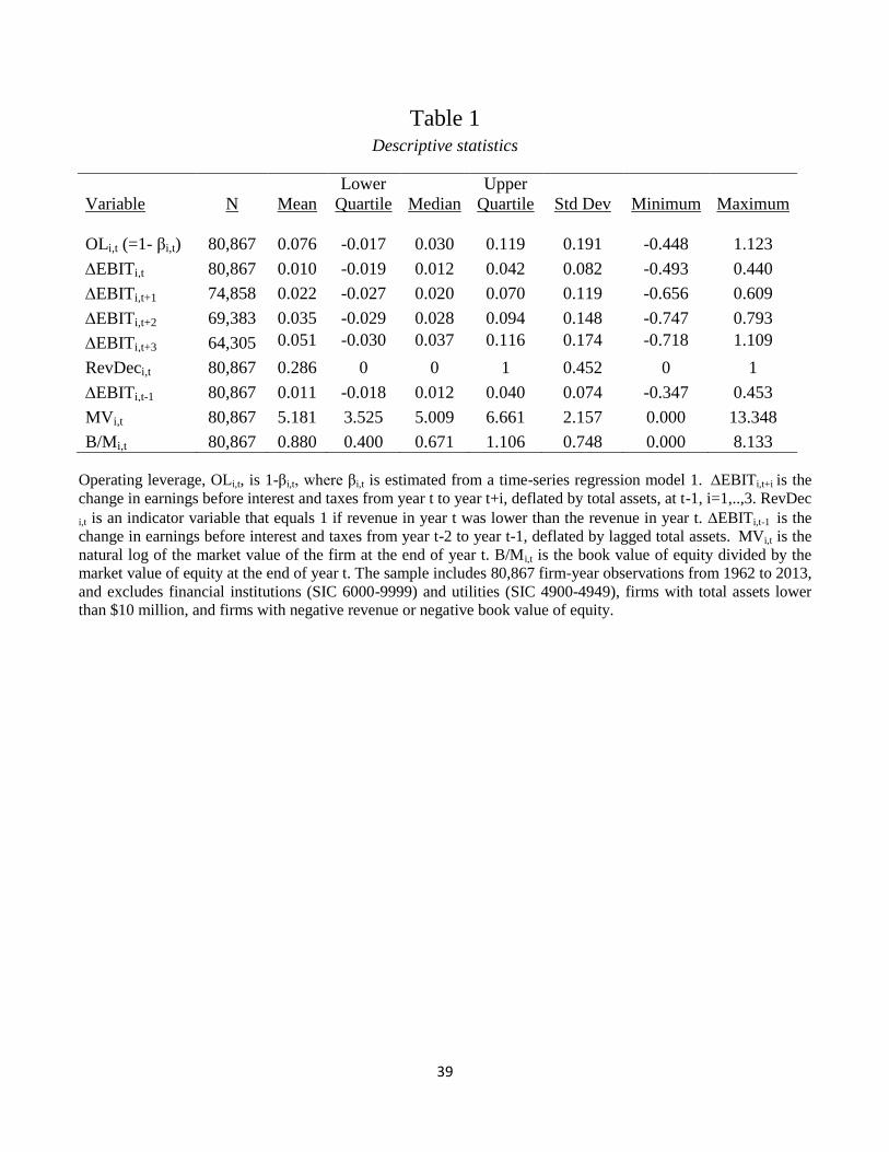
39

Table 1 Descriptive statistics

Lower

Upper

Variable N Mean Quartile Median Quartile Std Dev Minimum Maximum

OLi,t (=1- βi,t) 80,867 0.076 -0.017 0.030 0.119 0.191 -0.448 1.123

EBITi,t 80,867 0.010 -0.019 0.012 0.042 0.082 -0.493 0.440

EBITi,t+1 74,858 0.022 -0.027 0.020 0.070 0.119 -0.656 0.609

EBITi,t+2 69,383 0.035 -0.029 0.028 0.094 0.148 -0.747 0.793

EBITi,t+3 64,305 0.051 -0.030 0.037 0.116 0.174 -0.718 1.109

RevDeci,t 80,867 0.286 0 0 1 0.452 0 1

EBITi,t-1 80,867 0.011 -0.018 0.012 0.040 0.074 -0.347 0.453

MVi,t 80,867 5.181 3.525 5.009 6.661 2.157 0.000 13.348

B/Mi,t 80,867 0.880 0.400 0.671 1.106 0.748 0.000 8.133

Operating leverage, OLi,t, is 1-βi,t, where βi,t is estimated from a time-series regression model 1. EBITi,t+i is the

change in earnings before interest and taxes from year t to year t+i, deflated by total assets, at t-1, i=1,..,3. RevDec

i,t is an indicator variable that equals 1 if revenue in year t was lower than the revenue in year t. EBITi,t-1 is the

change in earnings before interest and taxes from year t-2 to year t-1, deflated by lagged total assets. MVi,t is the

natural log of the market value of the firm at the end of year t. B/Mi,t is the book value of equity divided by the

market value of equity at the end of year t. The sample includes 80,867 firm-year observations from 1962 to 2013,

and excludes financial institutions (SIC 6000-9999) and utilities (SIC 4900-4949), firms with total assets lower

than $10 million, and firms with negative revenue or negative book value of equity.

40

Table 2 Operating leverage increases earnings volatility and downside - Portfolio analysis

Revenue Falls

Lower quartile of revenue shocks

EBITi,t EBITi,t+1 EBITi,t+2 EBITi,t+3

(1) (2) (3) (4)

Operating

Leverage

OL

L -0.023 -0.009 0.006 0.019

M -0.035 -0.025 -0.010 0.003

H -0.045 -0.034 -0.016 -0.001

A

L

minus

H

0.023***

0.025***

0.022***

0.018***

Revenue Rises

Upper quartile of revenue shocks


Operating

Leverage

OL

L 0.054 0.074 0.087 0.102

M 0.058 0.077 0.093 0.115

H 0.067 0.083 0.091 0.108

B

L

minus

H

-0.014***

-0.009***

-0.004 -0.005

|A|-|B| 0.009***

0.016***

0.018***

0.013***

*, **

, and

*** are significant at 0.10, 0.05, and 0.01, respectively. T-test is used for testing the difference in means.

The table presents mean earnings growth for three portfolios sorted on operating leverage, conditioned on revenue

falls and revenue rises. Firms are sorted into three portfolios based on operating leverage at time t. Operating

leverage is a mean value of OL=1-β, where β is estimated from a time-series-regression model 1. Firms are also

independently sorted into four portfolios based on revenue growth (Revenuet - Revenuet-1)/Revenuet-1, and the

table presents the lower quartile and the upper quartile of revenue growth. For each portfolio, earnings growth is

presented for the three subsequent years relative to year t, EBITi,t+i = (EBITi,t+i- EBITi,t)/Assetsi,t-1, i=1,..,3. The

sample includes 80,867 observations from 1962 to 2013.

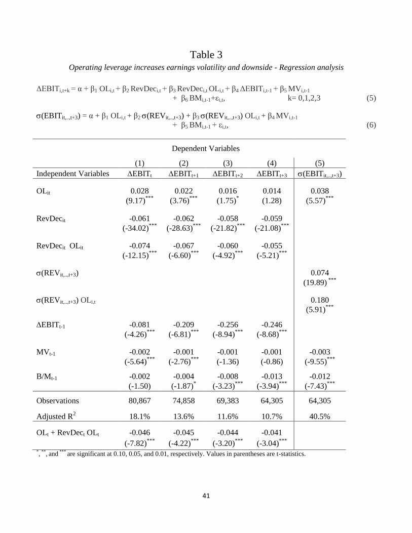
41

Table 3 Operating leverage increases earnings volatility and downside - Regression analysis

ΔEBITi,t+k = α + β1 OLi,t + β2 RevDeci,t + β3 RevDeci,t OLi,t + β4 ΔEBITi,t-1 + β5 MVi,t-1

+ β6 BMi,t-1+εi,t, k= 0,1,2,3 (5)

(EBITit,..,t+3) = α + β1 OLi,t + β2 (REVit,..,t+3) + β3 (REVit,..,t+3) OLi,t + β4 MVi,t-1

+ β5 BMi,t-1 + εi,t, (6)

Dependent Variables

(1) (2) (3) (4) (5)

Independent Variables EBITt EBITt+1 EBITt+2 EBITt+3 (EBITit,..,t+3)

OLit 0.028 0.022 0.016 0.014 0.038

(9.17)***

(3.76)***

(1.75)* (1.28) (5.57)

***

RevDecit -0.061 -0.062 -0.058 -0.059

(-34.02)***

(-28.63)***

(-21.82)***

(-21.08)***

RevDecit OLit -0.074 -0.067 -0.060 -0.055

(-12.15)***

(-6.60)***

(-4.92)***

(-5.21)***

(REVit,..,t+3)

0.074

(19.89) ***

(REVit,..,t+3) OLi,t

0.180

(5.91)***

EBITt-1 -0.081 -0.209 -0.256 -0.246

(-4.26)***

(-6.81)***

(-8.94)***

(-8.68)***

MVt-1 -0.002 -0.001 -0.001 -0.001 -0.003

(-5.64)***

(-2.76)***

(-1.36) (-0.86) (-9.55)***

B/Mt-1 -0.002 -0.004 -0.008 -0.013 -0.012

(-1.50) (-1.87)* (-3.23)

*** (-3.94)

*** (-7.43)

***

Observations 80,867 74,858 69,383 64,305 64,305

Adjusted R2

18.1% 13.6% 11.6% 10.7% 40.5%

OLt + RevDect OLt -0.046 -0.045 -0.044 -0.041

(-7.82)***

(-4.22)***

(-3.20)***

(-3.04)***

*, **

, and

*** are significant at 0.10, 0.05, and 0.01, respectively. Values in parentheses are t-statistics.

42

Table 4 Future expense changes - Regression analysis

ΔEXPi,t+k = α + β1 OLi,t + β2 RevDeci,t + β3 RevDeci,t OLi,t + β4 ΔEBITi,t-1 + β5 MVi,t-1

+ β6 BMi,t-1+εi,t, k= 0,1,2,3 (7)

Dependent Variables

(1) (2) (3) (4)

Independent Variables EXPt EXPt+1 EXPt+2 EXPt+3

OLt -0.025 -0.037 -0.038 -0.035

(-2.61)***

(-1.88)* (-1.20) (-0.84)

RevDect -0.340 -0.476 -0.555 -0.629

(-34.69)***

(-33.79)***

(-31.71)***

(-29.87)***

RevDect OLt 0.127 0.175 0.185 0.151

(8.45)***

(6.09)***

(4.17)***

(2.62)***

EBITt-1 0.499 0.874 1.317 1.748

(10.54)***

(9.68)***

(9.69)***

(10.67)***

MVt-1 -0.009 -0.017 -0.028 -0.042

(-4.95)***

(-5.07)***

(-5.65)***

(-6.40)***

B/Mt-1 -0.042 -0.095 -0.155 -0.222

(-8.00)***

(-7.68)***

(-8.27)***

(-8.43)***

Observations 80,867 74,858 69,383 64,305

Adjusted R2

34.2% 26.6% 23.0% 21.2%

OLt + RevDect OLt 0.102 0.138 0.147 0.116

(10.00)***

(6.44)***

(4.41)***

(2.39)**

*,, **

, and

*** are significant at 0.10, 0.05, and 0.01, respectively. Values in parentheses are t-statistics.

This table estimates the relation between operating leverage and future earnings growth. Operating leverage, OL,

is 1-β, where β is estimated from a time-series-regression model 1. EBITi,t+i is the change in earnings before

interest and taxes from year t to year t+i, i=0,..,3, deflated by total assets at t-1. (EBITi,t,..,t+3) is the standard

deviation of earnings before interest and taxes from year t to year t+i, i=0,..,3, deflated by total assets at t-1.

EXPt+i is the change in operating expenses from year t to year t+i, i=1,..,3, deflated by total assets at t-1, and

operating expenses are revenue minus earnings before interest and taxes. RevDec i,t is an indicator variable that

equals 1 if revenue in year t was lower than revenue in year t-1. EBITt-1 is the change in earnings before interest

and taxes from year t-2 to year t-1, deflated by lagged total assets. MVi,t is the natural log of the market value of

the firm at the end of year t. B/Mi,t is the book value of equity divided by the market value of equity at the end of

year t. The sample includes 80,867 observations from 1962 to 2013. Regression is estimated with industry (12-

industry classification from Fama and French (1997)) and year fixed effects. Errors are clustered on year and firm.

43

Table 5 Two consecutive revenue decreases vs. revenue increases

Two Consecutive Revenue Decreases

Revenuet+1<Revenuet<Revenuet-1


(1) (2) (3) (4)

Operating

Leverage

OL

L -0.023 -0.032 -0.020 -0.004

M -0.039 -0.055 -0.040 -0.025

H -0.046 -0.072 -0.057 -0.037

A

L

minus

H

0.023***

0.040***

0.036***

0.033***

Two Consecutive Revenue Increases

Revenuet+1>Revenuet>Revenuet-1


Operating

Leverage

OL

L 0.026 0.051 0.065 0.079

M 0.028 0.057 0.073 0.090

H 0.037 0.075 0.085 0.099

B

L

minus

H

-0.011***

-0.025***

-0.021***

-0.021***

|A|-|B| 0.012***

0.015***

0.016***

0.012**

*,, **

, and

*** are significant at 0.10, 0.05, and 0.01, respectively. T-test is used for testing the difference in means.

The table presents mean earnings growth for three portfolios sorted on operating leverage, and revenue increases

and decreases. Firms are sorted into three portfolios based on operating leverage at time t. Operating leverage is a

mean value of OL=1-β, where β is estimated from a time-series-regression model 1. Firms are also sorted into

two portfolios based on their revenue growth—firms that had a revenue decrease both at year t and t+1, and firms

that had a revenue increase both at year t and t+1. For each portfolio, earnings growth is presented for the three

subsequent years relative to year t, EBITi,t+i = (EBITi,t+i- EBITi,t)/Assetsi,t-1, i=1,..,3. The sample includes 80,867

observations from 1962 to 2013, and excludes financial institutions (SIC 6000-9999) and utilities (SIC 4900-

4949).

44

Table 6

Change in top five executives’ option compensation following FAS 123R

Change from

2000-2003

to 2004-2007

All Firms Change in Value of Options of Top Five Executives

Below Median Above Median

Difference test (one-

sided)

(1) (2) (3) (2) - (3)

ΔOptions Portfolio -0.082 -0.113 -0.052 -0.061***

(-15.78)***

(-14.65)***

(-7.89)***

ΔOptions Awards -0.106 -0.130 -0.081 -0.049***

(-16.17)***

(-14.15)***

(-8.96)***

ΔSalary -0.031 -0.004 -0.057 0.053***

(-6.13)***

(-0.57) (-9.38)***

ΔBonus -0.035 -0.033 -0.037 0.004

(-9.55)***

(-6.19)***

(-7.34)***

ΔRestricted Stocks 0.113 0.115 0.110 0.005

(19.60)***

(13.92)***

(13.77)***

ΔLTIA 0.015 0.007 0.024 -0.017***

(5.24)***

(2.01)**

(5.06)***

ΔOther 0.044 0.046 0.042 0.004

(6.89)***

(5.61)***

(4.28)***

Number of Firms 567 283 284 *, **

, and

*** indicate significance at 0.10, 0.05, and 0.01 levels, respectively. The values in parentheses are t-statistics.

The table presents the change in the compensation of the top five executives around FAS 123R. The change (Δ) in

each compensation component is the difference between the mean value during the pre-FAS 123R period, 2000-

2003, and the post-FAS 123R period, 2004-2007. Options Portfolio is the value of all options, vested and

unvested, divided by the value of all the options and stocks. Options Awards is the value of option awards divided

by total compensation. Salary is the dollar value of salary divided by total compensation. Bonus is the dollar value

of the bonus divided by total compensation. Restricted Stocks is the dollar value of stock awards divided by total

compensation. LTIA is the amount paid out to the executive under the company's long-term incentive plan

divided by total compensation. Other is all other compensation components, calculated as 1 minus (Options +

Salary + Bonus + Restricted Stocks + LTIA). The table presents the mean for all 567 sample firms, and for

sample firms with below/above median change in value of all options of the top five executives from the pre-FAS

123R period, 2000-2003, to the post-FAS 123R period, 2004-2007.

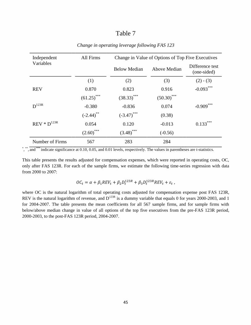
45

Table 7

Change in operating leverage following FAS 123

Independent

Variables

All Firms Change in Value of Options of Top Five Executives


Difference test

(one-sided)

(1) (2) (3) (2) - (3)

REV 0.870 0.823 0.916 -0.093***

(61.25)***

(38.33)***

(50.30)***

D123R

-0.380 -0.836 0.074 -0.909***

(-2.44)**

(-3.47)***

(0.38)

REV * D123R

0.054 0.120 -0.013 0.133***

(2.60)***

(3.48)***

(-0.56)

Number of Firms 567 283 284

*, **

, and


This table presents the results adjusted for compensation expenses, which were reported in operating costs, OC,

only after FAS 123R. For each of the sample firms, we estimate the following time-series regression with data

from 2000 to 2007:

,

where OC is the natural logarithm of total operating costs adjusted for compensation expense post FAS 123R,

REV is the natural logarithm of revenue, and D123R

is a dummy variable that equals 0 for years 2000-2003, and 1

for 2004-2007. The table presents the mean coefficients for all 567 sample firms, and for sample firms with

below/above median change in value of all options of the top five executives from the pre-FAS 123R period,

2000-2003, to the post-FAS 123R period, 2004-2007.

46

Table 8 Sensitivity analysis - Change in operating leverage based on change in CEO options

Independent

Variables

All Firms Change in Value of Options of CEO


Difference test (one-

sided)

(1) (2) (3) (2) - (3)

REV 0.870 0.835 0.904 -0.069**

(61.25)***

(39.30)***

(48.45)***

D123R

-0.380 -0.735 -0.027 -0.708**

(-2.44)**

(-3.21)***

(-0.13)

REV * D123R

0.054 0.110 -0.003 0.113***

(2.60)***

(3.30)***

(-0.12)

Number of firms 567 283 284

*, **

, and


For each of sample firms, we estimate the following time-series regression with data from 2000 to 2007:

,




for 2004-2007. The table presents the mean coefficients for all 567 sample firms, and for sample firms with

below/above median change in value of all options of the top five executives from the pre-FAS 123R period,

2000-2003, to the post-FAS 123R period, 2004-2007.

47

Table 9 Effect of the change in pay-performance sensitivity (delta) and convexity (vega) on operating leverage

following FAS 123R

Panel A: Effect of pay-performance convexity (vega) on operating leverage

Independent

Variables

Change in Vega of Top Five Executives


Difference Test (one-

sided)

(1) (2) (1) – (2)

REV 0.855 0.884 -0.029

(40.88)***

(46.03)***

D123R

-0.620 -0.141 -0.478

(-2.65)***

(-0.69)

REV * D123R

0.089 0.018 0.071*

(2.73)***

(0.73)

Number of firms 283 284

*, **

, and


Panel B: Effect of pay-performance sensitivity (delta) on operating leverage

Independent

Variables

Change in Delta of Top Five Executives


Difference Test (one-

sided)

(1) (2) (1) – (2)

REV 0.834 0.906 -0.072**

(37.31)***

(52.27)***

D123R

-1.003 0.240 -1.243***

(-4.06)***

(1.32)

REV * D123R

0.142 -0.034 0.176***

(4.18)***

(-1.53)

Number of firms 283 284

*, **

, and


48

Table 9 - Continued

We estimate the operating leverage for each of the sample firms, using the following time-series regression with

data from 2000 to 2007:

,




for 2004-2007. The table presents the mean coefficients for firms with high and low changes in vega (in Panel A),

and for high and low of changes in delta. Vega is the change in the value of the portfolio of options of the top five

executives for a 0.01 increase in the annualized standard deviation of a firm's stock returns. Delta is the change in

the value of the portfolio of stock and options of the top five executives for a 0.01 increase in the firm's stock

returns. The percent change in vega and delta are calculated from the pre-FAS 123R period, 2000-2003, to the

post-FAS 123R period, 2004-2007, respectively. Panel A presents the mean coefficients for firms with

below/above median change in vega of the top five executives, and Panel B presents the mean coefficients for

firms with below/above median change in delta of the top five executives.

49

Table 10 Sensitivity analysis - Changes in cost components following FAS 123R

Independent

Variables

All Firms Change in Value of All Options of Top Five Executives


Difference Test

(one-sided)

(1) (2) (3) (2) - (3)

Panel A:

REV 0.952 0.928 0.976 -0.048

(40.62)***

(25.50)***

(33.02)***

D123R

-0.181 -0.491 0.126 -0.617

(-0.76) (-1.21) (0.49)

REV * D123R

0.028 0.071 -0.014 0.086*

(0.99) (1.51) (-0.44)


Panel B:

REV 0.714 0.625 0.805 -0.180***

(18.93)***

(12.75)***

(14.11)***

D123R

-0.675 -1.036 -0.309 -0.727

(-2.00)**

(-2.44)**

(-0.59)

REV * D123R

0.108 0.163 0.052 0.111*

(2.46)***

(2.73)***

(0.81)


Panel C:

REV 0.451 0.347 0.557 -0.210

(5.26)***

(2.69)***

(5.05)***

D123R

-2.971 -4.183 -1.751 -2.433*

(-3.52)***

(-3.09)***

(-1.74)*

REV * D123R

0.267 0.314 0.220 0.384*

(3.49)***

(3.11)***

(1.65)*

Number of firms 307 154 153 *, **

, and


50

Table 10 - Continued

We estimate the operating leverage for each of sample firms, using the following time-series regression with data

from 2000 to 2007:

,

where COMPONENT is either COGS, SG&A, or R&D. COGS is the natural logarithm of cost of goods sold,

SG&A is the natural logarithm of sales general and administrative costs, and R&D is the natural logarithm of

research and development costs. REV is the natural logarithm of revenue, and D123R

is a dummy variable that

equals 0 for years 2000-2003, and 1 for 2004-2007. The panels present the mean coefficients for all sample firms

with available cost components data, and for sample firms with below/above median change in value of all

options of the top five executives from the pre-FAS 123R period, 2000-2003, to the post-FAS 123R period, 2004-

2007.

executive compensation and operating leverage

Documents