open access downstream prediction using a nonlinear ... · downstream prediction using a nonlinear...

HESSD10, 14331–14354, 2013

Downstreamprediction

N. H. Adenan andM. S. M. Noorani

Title Page

Abstract Introduction

Conclusions References

Tables Figures

J I

J I

Back Close

Full Screen / Esc

Printer-friendly Version

Interactive Discussion

Discussion

Paper

|D

iscussionP

aper|

Discussion

Paper

|D

iscussionP

aper|

Hydrol. Earth Syst. Sci. Discuss., 10, 14331–14354, 2013www.hydrol-earth-syst-sci-discuss.net/10/14331/2013/doi:10.5194/hessd-10-14331-2013© Author(s) 2013. CC Attribution 3.0 License.

Hydrology and Earth System

Sciences

Open A

ccess

Discussions

This discussion paper is/has been under review for the journal Hydrology and Earth SystemSciences (HESS). Please refer to the corresponding final paper in HESS if available.

Downstream prediction using a nonlinearprediction methodN. H. Adenan1 and M. S. M. Noorani2

1Universiti Pendidikan Sultan Idris, Perak, Malaysia2Universiti Kebangsaan Malaysia, Selangor, Malaysia

Received: 1 October 2013 – Accepted: 6 November 2013 – Published: 22 November 2013

Correspondence to: N. H. Adenan ([email protected])

Published by Copernicus Publications on behalf of the European Geosciences Union.

14331

http://www.hydrol-earth-syst-sci-discuss.net

http://www.hydrol-earth-syst-sci-discuss.net/10/14331/2013/hessd-10-14331-2013-print.pdf

http://www.hydrol-earth-syst-sci-discuss.net/10/14331/2013/hessd-10-14331-2013-discussion.html

http://creativecommons.org/licenses/by/3.0/

HESSD10, 14331–14354, 2013



Title Page



Tables Figures

J I

J I

Back Close

Full Screen / Esc



Discussion

Paper

|D

iscussionP

aper|

Discussion

Paper

|D

iscussionP

aper|

Abstract

The estimation of river flow is significantly related to the impact of urban hydrology,as this could provide information to solve important problems, such as flooding down-stream. The nonlinear prediction method has been employed for analysis of four yearsof daily river flow data for the Langat River at Kajang, Malaysia, which is located in5

a downstream area. The nonlinear prediction method involves two steps; namely, thereconstruction of phase space and prediction. The reconstruction of phase space in-volves reconstruction from a single variable to the m-dimensional phase space in whichthe dimension m is based on optimal values from two methods: the correlation dimen-sion method (Model I) and false nearest neighbour(s) (Model II). The selection of an10

appropriate method for selecting a combination of preliminary parameters, such asm, is important to provide an accurate prediction. From our investigation, we gatherthat via manipulation of the appropriate parameters for the reconstruction of the phasespace, Model II provides better prediction results. In particular, we have used ModelII together with the local linear prediction method to achieve the prediction results for15

the downstream area with a high correlation coefficient. In summary, the results showthat Langat River in Kajang is chaotic, and, therefore, predictable using the nonlinearprediction method. Thus, the analysis and prediction of river flow in this area can pro-vide river flow information to the proper authorities for the construction of flood control,particularly for the downstream area.20

1 Introduction

Urbanization and urban growth are essential factors for planners and policy makers be-cause the urbanization pattern has major implications for the hydrological processes.Urbanization can have various effects on certain hydrological problems, such as floodprevention in urban areas, allocation of adequate resources in terms of water qual-25

ity and quantity, and waterborne waste disposal (Hall, 1984). Thus, the problems of

14332





HESSD10, 14331–14354, 2013



Title Page



Tables Figures

J I

J I

Back Close

Full Screen / Esc



Discussion

Paper

|D

iscussionP

aper|

Discussion

Paper

|D

iscussionP

aper|

urban hydrology involve flood and pollution prevention. However, our study only con-siders flood prevention based on the river flow prediction. If an undeveloped area isthen transformed into a developed area, the conditions of the soil structure will be dis-turbed (Hall, 1984). These factors can change the magnitude of the river flow. Thevolume of runoff will increase significantly with the increase in the magnitude of the5

river flow due to the impervious areas and the lack of drainage. Hence, downstreamflooding problems exist in urban areas. There are several methods that can be usedto estimate the river flow in a watershed that is located in an urban area, such as theempirical and physical process methods. Referring to the empirical method for urbanhydrology research, the behaviour of river flow in the downstream area is important to10

provide accurate information for the whole river flow (Viesmann and Lewis, 1996). Thisinformation can help in planning, development and flood prevention of the downstreamarea.

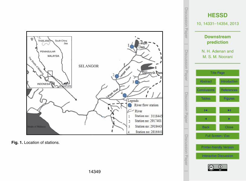
The Langat River, which is one of the longest rivers in the state of Selangor, Malaysia,is used as a case study. This research focuses on the downstream area at Kajang,15

which is well-known for experiencing flood hazards. Figure 1 shows the four gaugingstations along the Langat River. The Langat River flows from east to southeast, whichis from Lui River to Kajang. The total length of the upstream and downstream is about34.4 km and the downstream area has been identified as a flood risk area (Mohammedet al., 2011). Checkpoint 1 (station number 3118445) is located at the Lui River gaug-20

ing station (upstream) and Checkpoint 2 (station number 2917401) is located at theKajang gauging station (downstream). The Langat River at the Kajang gauging stationhas been used for the river flow analysis and prediction using the nonlinear predictionmethod. This area had a population of 229 655 people in 2000, which increased to342 657 people in 2010 (Department of Irrigation and Drainage Malaysia, 2005). The25

increase in population in this area reflects the development in the Kajang area. Further-more, the study area is adjacent to an industrial area and pig farms. Flooding in thisarea can cause damage to the industrial area and pollution in the Langat River basin.Thus, studies of the downstream area (Kajang) are important to provide information

14333





HESSD10, 14331–14354, 2013



Title Page



Tables Figures

J I

J I

Back Close

Full Screen / Esc



Discussion

Paper

|D

iscussionP

aper|

Discussion

Paper

|D

iscussionP

aper|

about the flow downstream. This study was conducted at this point so that the releaseof water from Checkpoint 2 could be estimated for a certain length of time. The resultsof this study could help to identify the preventive measures that could be undertaken inthis downstream area.

The analysis and prediction of river flow could provide the information about the dy-5

namics of the river flow system. However, the flow of the river is not dependent onrainfall alone. The characteristics of an area, such as shape, slope, land, soil struc-ture and climate change, can also affect the flow of the river in an area (Viesmannand Lewis, 1996). Thus, the application of stochastic methods is often used to anal-yse complex natural conditions, such as the river flow. Developments in the study of10

nonlinear time series analysis is growing with some revolutionary methods. One partic-ular method that provides important findings is known as chaos theory, which explainsthat a complex system can be analysed by deterministic methods that use a minimumnumber of the system’s variables (Islam and Sivakumar, 2002). Several decades ago,a number of studies were performed to obtain information on characterizing, modelling15

and predicting hydrological phenomena as a deterministic system (e.g. Jayawardenaand Lai, 1993; Sivakumar, 2000; Ghorbani et al., 2010). The results showed that theriver flow prediction and other hydrological processes are in good agreement with theactual data values (Sivakumar, 2003; Regonda et al., 2005; She and Yang, 2010; Khat-ibi et al., 2012). In addition, prediction using chaos theory can reveal the number of20

variables that affect the dynamics of the river flow.Studies on river flow analysis and prediction in Malaysia have been done and im-

proved for a variety of purposes, such as providing information for flood prevention.Several methods, such as support vector machine method (Shabri and Suhartono,2012), neural network model (Ahmad and Juahir, 2006) and hydrodynamic modelling25

(Ghani et al., 2010), have been used for river flow prediction. However, several meth-ods have yet to be explored for the purpose of river flow prediction in Malaysia, suchas chaos theory, Bayesian methods and wavelet methods. River flow prediction usingchaos theory involves a single variable (river flow data) albeit there are other dominant

14334





HESSD10, 14331–14354, 2013



Title Page



Tables Figures

J I

J I

Back Close

Full Screen / Esc



Discussion

Paper

|D

iscussionP

aper|

Discussion

Paper

|D

iscussionP

aper|

variables affecting river flow prediction. Meanwhile, the Bayesian and Wavelet meth-ods are dependent on a number of dominant variables, such as rainfall, temperatureand soil type. To the best of our knowledge, this is the first attempt to use the for theanalysis and prediction of river flow in Malaysia.

2 Nonlinear prediction method5

The nonlinear prediction method (NLP) of chaos theory is used to analyse river flowand predict the future value of the flow. There are two steps in NLP – phase spacereconstruction and prediction. Reconstruction of the phase space uses observed data(one-dimensional) to build the m-dimensional phase space that reflects the dynamicsof the river flow (Abarbanel, 1996; Adenan and Noorani, 2013). A scalar time series10

x(t) forms a one-dimensional time series:

{xi} = {x1,x2,x3, . . . ,xN} (1)

where N is the total number of points in the time series that can be transformed intom-dimensional vectors:

Y t ={xt,xt+τ,xt+2τ, . . . ,xt+(m−1)τ

}(2)15

where τ is an appropriate time delay and m is a chosen embedding dimension (Abar-banel, 1996; Tongal and Berndtsson, 2013).

Referring to Eq. (2), the value of τ and m are needed to reconstruct the phase space.In this study, τ has been predetermined. Selection of the appropriate τ is importantduring the reconstruction of the phase space. The most optimal value of τ can provide20

a separation of neighbouring projections with respect to the dimension of the phasespace. If the value of τ is too small, the coordinates of the phase space cannot properlydescribe the dynamics of the system. Meanwhile, information on trajectories in thephase space will diverge if the value of τ is too big (Sangoyomi et al., 1996; Islam and

14335





HESSD10, 14331–14354, 2013



Title Page



Tables Figures

J I

J I

Back Close

Full Screen / Esc



Discussion

Paper

|D

iscussionP

aper|

Discussion

Paper

|D

iscussionP

aper|

Sivakumar, 2002). The optimal value of m in phase space reconstruction can describethe topology of the attractor. The number of dimensions in the reconstructed phasespace is equal to the number of columns in the matrix resulting from the embeddingparameters in the time series. If the number of columns is insufficient, it cannot reflectthe phase space dynamics of the system. Therefore, the selection of the preliminary5

parameter pair (τ,m) is important to reflect the dynamics of the phase space.

2.1 Determination of preliminary parameter pair (τ,m)

Previous studies on the river flow prediction showed that when a condition of time delayτ = 1 is used in phase space reconstruction, the results gave good predictions (Sivaku-mar, 2002, 2003). Thus, in this study, the time delay τ = 1 is used. The embedding10

dimension m is calculated using the correlation dimension and false nearest neighbourmethod (FNN). There are two models to be considered, Model I and Model II, whichinvolve different combinations of preliminary parameter pairs for the reconstruction ofthe phase space. Model I involves τ = 1, and m is the result of the calculation fromthe correlation dimension; and Model II involves the combination τ = 1, and m is the15

result of the calculation of FNN. A comparison of the prediction results is conducted todistinguish the strength of the two models.

The correlation dimension method is the most fundamental method in the study ofchaotic time series for proving the presence of chaotic behaviour in hydrological stud-ies (Jayawardena and Lai, 1994; Martins et al., 2011; Khatibi et al., 2012). For a given20

distance r , the main idea of the correlation function C(r) is related to the shortest dis-tance of the vectors Y t. Here the Euclidean distance is used to calculate the distancebetween points on the vector space:

ds(Y i ,Y j ) = ‖Y i −Y j‖. (3)

14336





HESSD10, 14331–14354, 2013



Title Page



Tables Figures

J I

J I

Back Close

Full Screen / Esc



Discussion

Paper

|D

iscussionP

aper|

Discussion

Paper

|D

iscussionP

aper|

The correlation dimension is based on the correlation integral introduced by Grass-berger (1986):

C(r) = limN→∞

2N(N −1)

N∑i ,j=1

H(r −‖Y i −Y j‖) (4)

where H is the Heavyside function, which has the value 0 or 1 and can be defined as:

H(r −‖Y i −Y j‖) ={

1,0 ≤ (r −‖Y i −Y j‖)0,0 > (r −‖Y i −Y j‖)

(5)5

and acts as a barrier to the Euclidean distance between two points on the attractor Y iand Y j . The correlation function C(r) is calculated for the pair of points (Y i ,Y j ) witha distance less than the radius r . In the limit to infinite amount of data (N →∞) andsufficiently small r(r → 0), the relation C(r) ∼= αrD2 is expected (Men et al., 2004). The10

correlation dimension D2 and correlation exponent v can be defined as:

D2 = limr→0

v (6)

v =δ[logC(r)]

δ[logr ](7)

Several steps are required to identify the value of the correlation dimension. The first15

step is to draw a graph lnC(r) vs. ln(r) with a given m. Then the gradient (correlationexponent v) of the m-dimensional curve values has to be determined. The gradient ofthe graph can be measured by the least squares method for determining the scaling.For finite data and where the value of r exceeds the diameter, there exists a saturatedarea of the graph. The saturated area is the scaling region. A better way to estimate20

the gradient is to use δ[logC(r)]/δ[logr ]. To examine if there is a chaotic nature, thecorrelation exponent (slope v) vs. m-dimensional has to be plotted. If the value of the

14337





HESSD10, 14331–14354, 2013



Title Page



Tables Figures

J I

J I

Back Close

Full Screen / Esc



Discussion

Paper

|D

iscussionP

aper|

Discussion

Paper

|D

iscussionP

aper|

correlation exponent is finite, low and non-integer, the system is considered to be oflow dimensional chaotic nature (Men et al., 2004). If the correlation value increaseswithout limit as m increases, the system should be studied as a stochastic system.

The false nearest neighbour method (FNN) is an effective method for finding theembedding dimension m for the reconstruction phase space. This method has been5

used to analyse river flow time series (Wu and Chau, 2010; Ghorbani et al., 2012).This paragraph describes how FNN is implemented. Suppose the dimension increasesthen the distance between the point and the nearest neighbour should not change ifit is indeed the nearest neighbouring point. Computation of the distance between thepoint and the nearest neighbour is by the Euclidean distance.10

FNN can be calculated using the following algorithm. Assumethat Y i =

{xi ,xi+τ,xi+2τ, . . . ,xi+(m−1)τ

}has nearest neighbour Y

NNi ={

xNNi ,xNN

i+τ,xNNi+2τ, . . . ,x

NNi+(m−1)τ

}. Then, calculate the Euclidean distance

∥∥∥Y i −YNNi

∥∥∥.

For all points i in vector space, equation|xi+mτ−x

NNi+mτ |

‖Y i−Y NNi ‖ > RT is used and the value of false

nearest neighbour can be calculated. RT is a value between 10 and 30. In this study,15

the value of 15 is used (Wu and Chau, 2010). Repeat the algorithm with differentembedding dimensions and the value of the false nearest neighbour that is close tozero is used as the embedding dimension.

2.2 Prediction

In this study, the prediction of river flow has been performed by using the local linear20

approximation method. This method was proposed by Lorenz (1969). Application of thelocal linear approximation method is to (1) examine whether the river flow at the down-stream areas can be predicted, (2) to compare the prediction results for Models I andII. The local linear approximation method is used to predict river flow in downstreamareas as follows. The first step is to reconstruct the phase space. The combination of25

the preliminary parameter pair (τ,m) is important for reconstruction of the phase space

14338





HESSD10, 14331–14354, 2013



Title Page



Tables Figures

J I

J I

Back Close

Full Screen / Esc



Discussion

Paper

|D

iscussionP

aper|

Discussion

Paper

|D

iscussionP

aper|

because this phase space result will be used in making a prediction. The differencebetween Models I and II is in the reconstruction phase space. Models I and II involveτ = 1 but involve different methods in determining the value of m. Model I uses the cor-relation dimension while FNN is employed for Model II. Assume that the reconstructionof phase space is like Y i =

{xi ,xi+τ,xi+2τ, . . . ,xi+(m−1)τ

}. The nearest neighbour for Y t5

is required to predict Y t+1. Assume that the vector of the minimum distance to thenearest neighbour is Y M . Next, for the local linear approximation method, the values ofY M and Y M+1 are used to satisfy the linear equations Y M+1 = AY M +B. The constantsA and B are calculated using the least squares method. Thus, the predictive value Y t+1can be calculated using Y t+1 = AY t +B.10

2.3 Performance evaluation

The assessment of the prediction accuracy of the models for predicting the daily riverflow is evaluated by using the mean absolute error (MAE), root mean square error(RMSE) and correlation coefficient (CC). The MAE, RMSE and CC are as follows:

MAE =1n

n∑t=1

∣∣∣yot − y f

t

∣∣∣ (8)15

RMSE =

√√√√1n

n∑t=1

(yot − y f

t

)2(9)

CC =

1n

∑nt=1

(yot − y

ot

)(y ft − y

ft

)√

1n

∑nt=1

(yot − y

ot

)2√

1n

∑nt=1

(y ft − y

ft

)2(10)

where yot is the observed and y f

t is the forecast value at time t, and n is the numberof data points. MAE and RMSE can provide information on the predictive ability of the20

14339





HESSD10, 14331–14354, 2013



Title Page



Tables Figures

J I

J I

Back Close

Full Screen / Esc



Discussion

Paper

|D

iscussionP

aper|

Discussion

Paper

|D

iscussionP

aper|

models involved. Meanwhile, the correlation coefficient CC can measure the correlationbetween the prediction and the observed data.

3 Description of data

Langat River is one of the longest rivers in Selangor and its river basin is transbound-ary, inasmuch as it crosses three states – Selangor, Negeri Sembilan, and the Fed-5

eral Territory of Kuala Lumpur and Putrajaya (Department of Irrigation and DrainageMalaysia, 2011).The Langat River flows from Mount Nuang in Hulu Langat district tothe Straits of Malacca in Kuala Langat. The Langat River catchment area covers a totalof 1815 km2 and is located between latitude 2◦40′152′′ N and 3◦16′15′′N, and longitude101◦19′20′′ E and 102◦1′10′′ E (Juahir et al., 2011). There are two water reservoirs lo-10

cated in this area – Langat Dam and Semenyih Dam. Langat Dam was built with anarea of 54 km2 and Semenyih Dam has an area of 41 km2. Both of these dams werebuilt to deliver water for domestic and industrial use. In addition, the Langat Dam is alsoused to generate electricity for the use of residents in the vicinity of the Langat Valley.There are several towns and villages built along the Langat River – Cheras, Semenyih,15

Dengkil and Kajang. Since 1976, Langat River has also been acknowledged to be anarea that regularly suffers flooding.

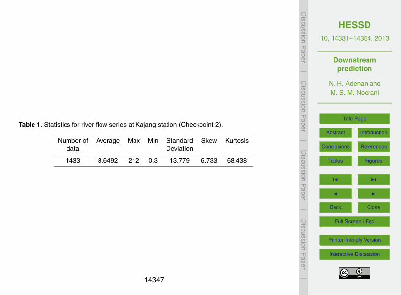
The variations of daily river flow data for Checkpoint 2 are shown in Fig. 2. Theirregular patterns in data for Kajang River show that the river in this area is a complexsystem. The overall data were taken from the Department of Irrigation and Drainage20

Malaysia. Missing data constitute about 0.018 % and were filled using the results oflinear interpolation calculation. The statistical parameters of the data cover a period offour years (January 2002 to December 2005) and are shown in Table 1.

14340





HESSD10, 14331–14354, 2013



Title Page



Tables Figures

J I

J I

Back Close

Full Screen / Esc



Discussion

Paper

|D

iscussionP

aper|

Discussion

Paper

|D

iscussionP

aper|

4 Results and Discussion

River flow prediction using NLP involves the reconstruction of the phase space andprediction. Thus, the discussion of the findings is divided into two parts. The first partis to determine the parameters for the reconstruction of the phase space for Models Iand II. Meanwhile, the description of the prediction results are discussed in the second5

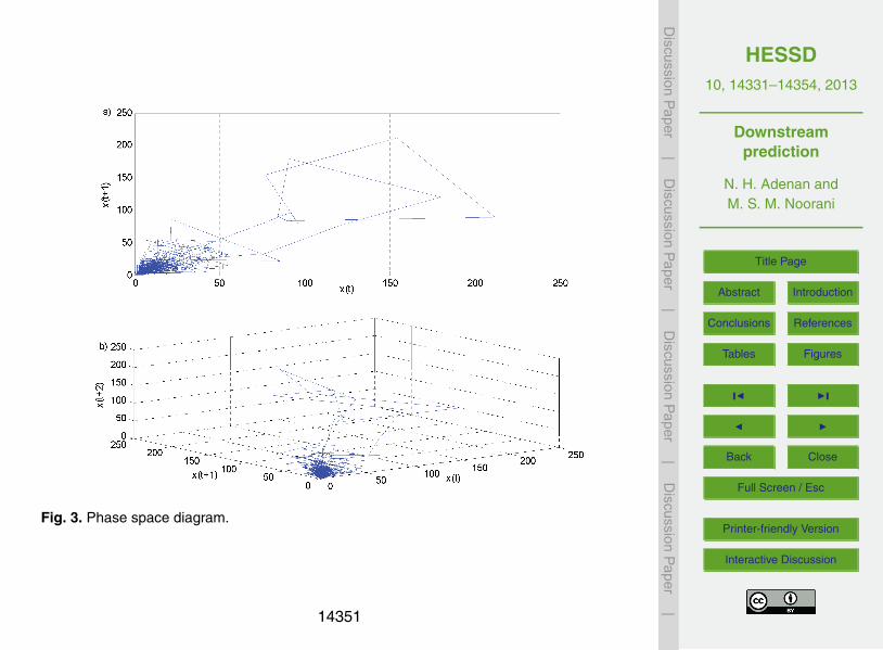
part.The phase diagram can provide information about the dynamics of a system through

the trajectories in the phase space. The trajectories that are of interest focus ona subspace called the attractor. In addition, the observation of attractor trajectoriesin the phase space can provide information about the chaotic behaviour of the sys-10

tem. Hence, the phase diagram and the observation data involved are plotted. Figure 3shows the phase diagram in two and three dimensions with τ = 1. The trajectories inthe phase space can indicate the presence of chaotic behaviour of the data (Sivaku-mar, 2002). Referring to Fig. 3, the trajectories of the attractor are clearly shown in thetwo phase diagrams. Thus, the data involved in this analysis are chaotic. Therefore, the15

dynamics of the system can be studied using chaos theory without involving stochasticmethods.

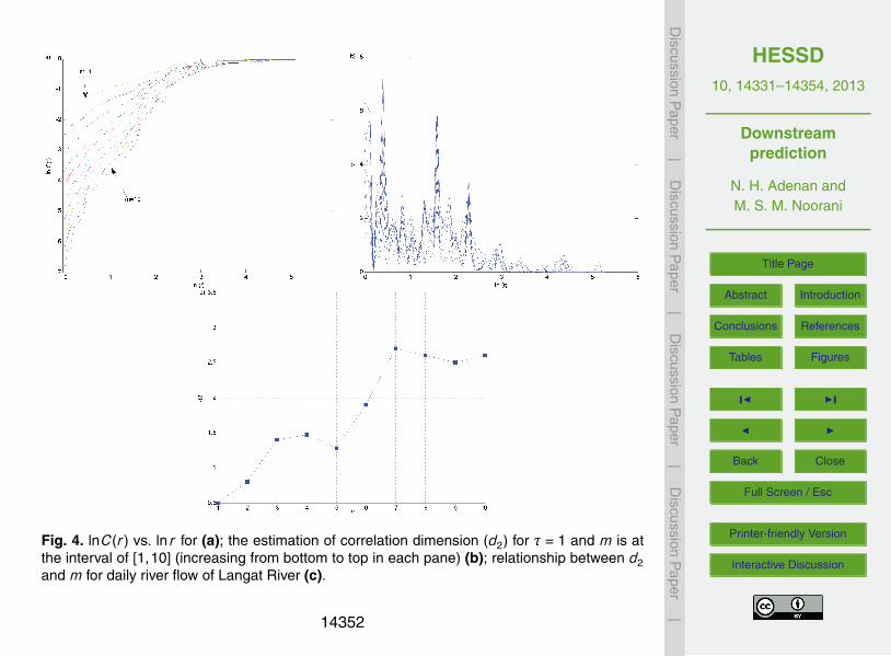
This study involved data from January 2002 to December 2005 (1433 days). Threeyears of data are used in the reconstruction of the phase space to predict the behaviourone year ahead. Reconstruction of the phase space is based on the embedding dimen-20

sion. In Model I, the embedding dimension is based on the calculation of the correlationdimension. Graph lnC(r) vs. ln(r) in Fig. 4a shows the behaviour of the correlation func-tion v vs. radius r for the increasing m-dimensional. In general, the increasing value ofthe m-dimensional gradient occurs at the beginning of the curve from left m = 1 to rightm = 10. Meanwhile, the graph of the correlation dimension estimation, the relationship25

between the correlation exponent v for different values of m is shown in Fig. 4b. Therelationship between the value of correlation dimension d2 and m-dimension can beseen in Fig. 4c, which is a graph of d2 vs. m. The value of the correlation dimension

14341





HESSD10, 14331–14354, 2013



Title Page



Tables Figures

J I

J I

Back Close

Full Screen / Esc



Discussion

Paper

|D

iscussionP

aper|

Discussion

Paper

|D

iscussionP

aper|

increased as the value of the m-dimensional increased. The increase in m-dimensioncan be seen up to a scaling region where the correlation dimension is saturated. Thesituation in which the value for the correlation dimension is saturated might indicate theexistence of deterministic dynamics in the system. The saturated conditions for the d2value is in the interval (2.5,3). The saturation value for d2 is known as the correlation di-5

mension attractor (Sivakumar, 2000). In general, the sufficient condition for the value ofthe smallest integer m is m greater than 2D2 (Wu and Chan, 2010). Thus, the value ofm = 6 is related to the Langat River flow time series in Kajang. The correlation dimen-sion d2 is finite and shows low levels of correlation dimension. Hence, Sungai Langat isa chaotic and deterministic system. Model I involves a combination of preliminary pa-10

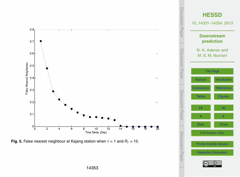
rameters (1,6) in the phase space reconstruction. Model II involves the calculation of musing FNN to find a combination of the preliminary parameters for RPS. Figure 5 showsthe percentage of false nearest neighbours vs. m. Thus, the optimal value for the em-bedding dimension identified is m = 14. Model II involves a combination of parameters(1,14) for the reconstruction phase space.15

4.1 River flow prediction for Model I and Model II

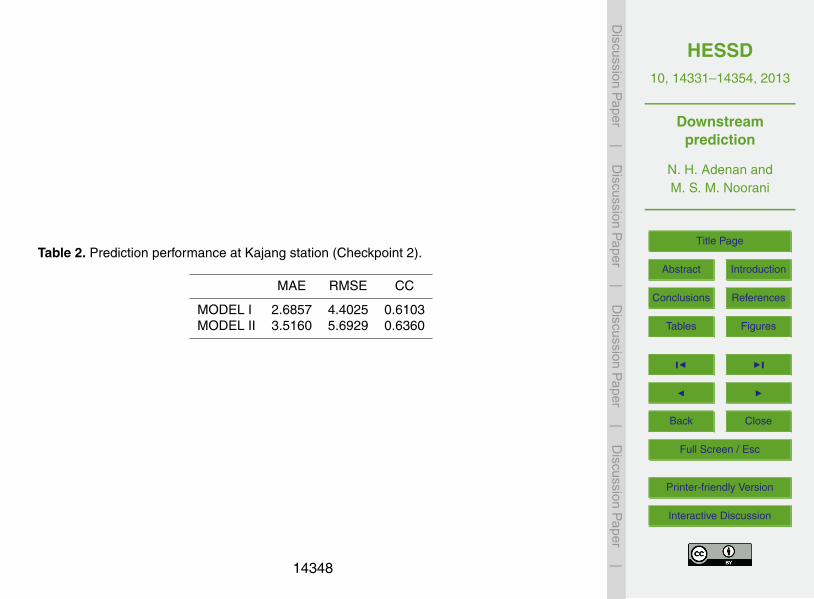
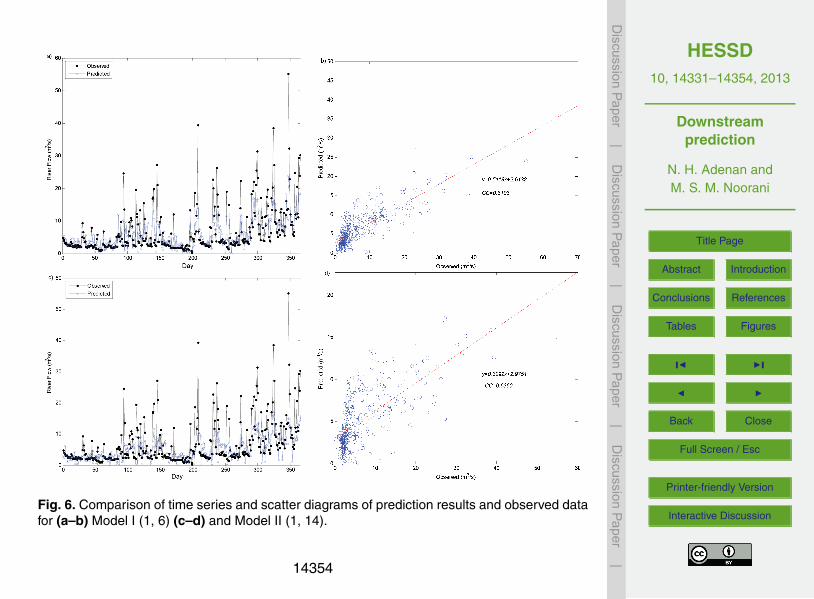
The combination of preliminary parameters for Model I is (1,6) while for Model II it is(1,14). Thus, for both models, the combination of the preliminary parameters (τ,m) hasbeen applied to construct the phase space. Figure 6 and Table 2 provide a summaryof the river flow prediction results in terms of MAE, RMSE and CC. Overall, the results20

show good performance prediction for chaos theory in predicting the future value ofthe river flow for the downstream area. Referring to Table 2, a comparison of predictionperformance shows that the prediction results for Model II are better than Model I.The correlation coefficient for Model II (0.6360) is slightly higher compared to Model I(0.6103). Thus, analysis and prediction of the Langat River can provide information in25

which the selection of a combination of preliminary parameters in the reconstructionphase space is essential for better prediction results. In this study, Model II uses FNN

14342





HESSD10, 14331–14354, 2013



Title Page



Tables Figures

J I

J I

Back Close

Full Screen / Esc



Discussion

Paper

|D

iscussionP

aper|

Discussion

Paper

|D

iscussionP

aper|

to calculate the embedding dimension m and is more appropriate than the correlationdimension method.

5 Conclusions

Analysis and prediction for testing the presence of chaotic behaviour in daily river flowdata recorded at Langat River involving the station at Kajang, Selangor, Malaysia, has5

been performed. The station is located in the downstream area, which is a flood pronearea. The analysis was carried out on the river flow data for a period of 4 yr (2002–2005). The focus of this study was to identify the chaotic behaviour of the river flowdata in the downstream area and determine whether the river flow can be predictedwhen chaotic behaviour of the river exists downstream. Chaos theory, together with10

NLP, were used in the analysis. The reconstruction phase space clearly shows theexistence of a chaotic attractor. Hence, the data involved in this analysis are chaotic.Next, was the attempt to make a prediction for one year ahead with the observeddata using the results of the reconstruction of the phase space for three years. Twocombinations of preliminary parameters were used. Model I used τ = 1 for which m is15

the result of the calculation of the correlation dimension, while Model II used τ = 1 forwhich m is the result of FNN calculation. Using these methods, the optimal combinationfor Model I was (1,6) and for Model II it was (1,14). The overall prediction resultsshowed that both models could give a good prediction for the river flow downstream.However, the combination of the preliminary parameters for Model II using the FNN20

algorithm provided a better prediction result than Model I, which used the correlationdimension. The results showed that Langat River in Kajang, which is in the downstreamarea, is chaotic and predictable using NLP. Therefore, the results of the analysis andprediction of river flow in the downstream area could provide information on river flowfor the authorities to take appropriate control of the downstream flooding.25

14343





HESSD10, 14331–14354, 2013



Title Page



Tables Figures

J I

J I

Back Close

Full Screen / Esc



Discussion

Paper

|D

iscussionP

aper|

Discussion

Paper

|D

iscussionP

aper|

Acknowledgements. The authors are grateful to Universiti Kebangsaan Malaysia for providingfinancial support via the grant UKM-DIP-2012-31.

References

Abarbanel, H. D. I.: Analysis of observed chaotic data, Springer-Verlag, Inc, New York, 1996.Adenan, N. H. and Noorani, M. S. M.: Behaviour of daily river flow: Chaotic?, Proceedings of the5

20th National Symposium on Mathematical Sciences: Research in Mathematical Sciences:A Catalyst for Creativity and Innovation, Malaysia, 221–228, 2013.

Ahmad, Z. and Juahir, H.: Neural Network Model for Prediction of Discharged from the Catch-ments of Langat River, Malaysia, IIUM Engineering Journal, 7, 25–34, 2006.

Department of Irrigation and Drainage Malaysia: Langat River Integrated River Basin Manage-10

ment Study, Final Report, Technical Studies Part 1 of 4, 2005.Department of Irrigation and Drainage Malaysia: Review of the National Water Resources

(2000–2050) and Formulation of National Water Resources Policy, Selangor, Federal Ter-ritory of Kuala Lumpur and Putrajaya, 2011.

Ghani, A. A., Ali, R., Zakaria, N. A., Hasan, Z. A., Chang, C. K., and Ahmad, M. S. S.: A15

Temporal Change Study of the Muda River System Over 22 Years, International Journal ofRiver Basin Management, 8, 25–37, 2010.

Ghorbani, M. A., Kisi, O., and Aalinezhad, M.: A probe into the chaotic nature of daily streamflowtime series by correlation dimension and largest Lyapunov methods, Appl. Math. Modell., 34,4050–4057, 2010.20

Ghorbani, M. A., Daneshfaraz, R., Arvanagi, H., and Pourzangbar, A.: Local Prediction in RiverDischarge Time Series, Online Journal of Civil Engineering and Urbanism, 2, 51–55, 2012.

Grassberger, P.: Do climatic attractors exist?, Nature, 323, 609–612, 1986.Hall, M. J.: Urban Hydrology, Elsevier Applied Science Publishers, New York, 1984.Islam, M. N. and Sivakumar, B.: Characterization and prediction of runoff dynamics: a nonlinear25

dynamical view, Adv. Water Res., 25, 179–190, 2002.Jayawardena, A. W. and Lai, F.: Chaos in hydrological time series, Proceeding of the Yokohama

Symposium – Extreme Hydrological Events: Precipitation, Floods and Droughts, Yokohama,59–66, 1993.

14344





HESSD10, 14331–14354, 2013



Title Page



Tables Figures

J I

J I

Back Close

Full Screen / Esc



Discussion

Paper

|D

iscussionP

aper|

Discussion

Paper

|D

iscussionP

aper|

Jayawardena, A. W. and Lai, F.: Analysis and prediction of chaos in rainfall and streamflow timeseries, J. Hydrol., 153, 23–52, doi:10.1016/0022-1694(94)90185-6, 1994.

Juahir, H., Zain, S. M., Yusoff, M. K., Hanidza, T. I. T., Armi, A. S. M., Toriman, M. E., andMokhtar, M.: Spatial water quality assessment of Langat River Basin (Malaysia) using envi-ronmetric techniques, Environ. Monit. Assess., 173, 625–641, 2011.5

Khatibi, R., Sivakumar, B., Ghorbani, M. A., Kisi, O., Kocak, K., and Zadeh, D. F.: Investigatingchaos in river stage and discharge time series, J. Hydrol., 414–415, 108–117, 2012.

Lorenz, E. N.: Atmospheric predictability as revealed by naturally occurring analogues, J. At-mos. Sci, 26, 636–646, 1969.

Martins, O. Y., Sadeeq, M. A., and Ahaneku, I. E.: Nonlinear Deterministic Chaos in Beneu10

River Flow Daily TIme Sequence, Journal of Water Resource and Protection, 3, 747–757,2011.

Men, B., Zhao, X., and Liang, C.: Chaotic analysis on monthly precipitation on Hills Region inMiddle Sichuan of China, Nature and Science, 2, 45–51, 2004.

Mohammed, T. A., Al-Hassoun, S., and Ghazali, A. H.: Prediction of flood levels a streacth of the15

Langat River with insufficient hydrological data, Pertanika Journal of Science & Technology,2, 237–248, 2011.

Regonda, S., Rajagopalan, B., Lall, U., Clark, M., and Moon, Y.-I.: Local polynomialmethod for ensemble forecast of time series, Nonlin. Processes Geophys., 12, 397–406,doi:10.5194/npg-12-397-2005, 2005.20

Sangoyomi, A., Lall, L., and Abarbanel, H. D. I.: Nonlinear dynamics of the Great Salt Lake:dimension estimation, Water Resour. Res., 32, 149–159, 1996.

Shabri, A. and Suhartono: Streamflow forecasting using least-squares support vector ma-chines, Hydrolog. Sci. J., 57, 1275–1293, doi:10.1080/02626667.2012.714468, 2012.

She, D. and Yang, X.: A New Adaptive Local Linear Prediction Method and Its Application25

in Hydrological Time Series, Math. Probl. Eng., 2010, 205438, doi:10.1155/2010/205438,2010.

Sivakumar, B.: Chaos theory in hydrology: important issues and interpretation, J. Hydrol., 227,1–20, 2000.

Sivakumar, B.: A phase-space reconstruction approach to prediction of suspended sediment30

concentration in rivers, J. Hydrol., 258, 149–162, 2002.Sivakumar, B.: Forecasting monthly streamflow dynamics in the western United States: a non-

linear dynamical approach, Environ. Modell. Softw., 18, 721–728, 2003.

14345





http://dx.doi.org/10.1016/0022-1694(94)90185-6

http://dx.doi.org/10.5194/npg-12-397-2005

http://dx.doi.org/10.1080/02626667.2012.714468

http://dx.doi.org/10.1155/2010/205438

HESSD10, 14331–14354, 2013



Title Page



Tables Figures

J I

J I

Back Close

Full Screen / Esc



Discussion

Paper

|D

iscussionP

aper|

Discussion

Paper

|D

iscussionP

aper|

Tongal, H. and Berndtsson, R.: Phase-space reconstruction and self-exciting threshold mod-eling approach to forecast lake water levels, Stoch. Env. Res. Risk. A., online first,doi:10.1007/s00477-013-0795-x, 2013.

Viessman, W. and Lewis, G. L.: Introduction to Hydrology, HarperCollins College Publishers,New York, 760 pp., 1996.5

Wu, C. L. and Chau, K. W.: Data driven for monthly streamflow time series prediction, Eng.Appl. Artif. Intel., 23, 1350–1367, 2010.

14346





http://dx.doi.org/10.1007/s00477-013-0795-x

HESSD10, 14331–14354, 2013



Title Page



Tables Figures

J I

J I

Back Close

Full Screen / Esc



Discussion

Paper

|D

iscussionP

aper|

Discussion

Paper

|D

iscussionP

aper|

Table 1. Statistics for river flow series at Kajang station (Checkpoint 2).

Number of Average Max Min Standard Skew Kurtosisdata Deviation

1433 8.6492 212 0.3 13.779 6.733 68.438

14347





HESSD10, 14331–14354, 2013



Title Page



Tables Figures

J I

J I

Back Close

Full Screen / Esc



Discussion

Paper

|D

iscussionP

aper|

Discussion

Paper

|D

iscussionP

aper|

Table 2. Prediction performance at Kajang station (Checkpoint 2).

MAE RMSE CC

MODEL I 2.6857 4.4025 0.6103MODEL II 3.5160 5.6929 0.6360

14348





HESSD10, 14331–14354, 2013



Title Page



Tables Figures

J I

J I

Back Close

Full Screen / Esc



Discussion

Paper

|D

iscussionP

aper|

Discussion

Paper

|D

iscussionP

aper|

Fig. 1. Location of stations.

14349





HESSD10, 14331–14354, 2013



Title Page



Tables Figures

J I

J I

Back Close

Full Screen / Esc



Discussion

Paper

|D

iscussionP

aper|

Discussion

Paper

|D

iscussionP

aper|

Fig. 2. Variations in data for Kajang station (Checkpoint 2).

14350





HESSD10, 14331–14354, 2013



Title Page



Tables Figures

J I

J I

Back Close

Full Screen / Esc



Discussion

Paper

|D

iscussionP

aper|

Discussion

Paper

|D

iscussionP

aper|

Fig. 3. Phase space diagram.

14351





HESSD10, 14331–14354, 2013



Title Page



Tables Figures

J I

J I

Back Close

Full Screen / Esc



Discussion

Paper

|D

iscussionP

aper|

Discussion

Paper

|D

iscussionP

aper|

Fig. 4. lnC(r) vs. lnr for (a); the estimation of correlation dimension (d2) for τ = 1 and m is atthe interval of [1,10] (increasing from bottom to top in each pane) (b); relationship between d2and m for daily river flow of Langat River (c).

14352





HESSD10, 14331–14354, 2013



Title Page



Tables Figures

J I

J I

Back Close

Full Screen / Esc



Discussion

Paper

|D

iscussionP

aper|

Discussion

Paper

|D

iscussionP

aper|

Fig. 5. False nearest neighbour at Kajang station when τ = 1 and RT = 15.

14353





HESSD10, 14331–14354, 2013



Title Page



Tables Figures

J I

J I

Back Close

Full Screen / Esc



Discussion

Paper

|D

iscussionP

aper|

Discussion

Paper

|D

iscussionP

aper|

Fig. 6. Comparison of time series and scatter diagrams of prediction results and observed datafor (a–b) Model I (1, 6) (c–d) and Model II (1, 14).

14354





open access downstream prediction using a nonlinear ... · downstream prediction using a nonlinear...

Documents