research article fault prediction for nonlinear system...

Research ArticleFault Prediction for Nonlinear System Using Sliding ARMACombined with Online LS-SVR

Shengchao Su,1,2 Wei Zhang,1 and Shuguang Zhao2

1 Laboratory of Intelligent Control and Robotics, Shanghai University of Engineering Science, Shanghai 201620, China2 College of Information Science and Technology, Donghua University, Shanghai 201620, China

Correspondence should be addressed to Shengchao Su; [email protected]

Received 3 April 2014; Accepted 7 June 2014; Published 16 July 2014

Academic Editor: Jingjing Zhou

Copyright © 2014 Shengchao Su et al. This is an open access article distributed under the Creative Commons Attribution License,which permits unrestricted use, distribution, and reproduction in any medium, provided the original work is properly cited.

A robust online fault predictionmethodwhich combines sliding autoregressivemoving average (ARMA)modelingwith online leastsquares support vector regression (LS-SVR) compensation is presented for unknown nonlinear system. At first, we design an onlineLS-SVR algorithm for nonlinear time series prediction. Based on this, a combined time series prediction method is developed fornonlinear system prediction.The sliding ARMAmodel is used to approximate the nonlinear time series; meanwhile, the online LS-SVR is added to compensate for the nonlinear modeling error with external disturbance. As a result, the one-step-ahead predictionof the nonlinear time series is achieved and it can be extended to n-step-ahead prediction.The result of the n-step-ahead predictionis then used to judge the fault based on an abnormity estimation algorithm only using normal data of system. Accordingly, theonline fault prediction is implemented with less amount of calculation. Finally, the proposed method is applied to fault predictionof model-unknown fighter F-16. The experimental results show that the method can predict the fault of nonlinear system not onlyaccurately but also quickly.

1. Introduction

Fault prediction mainly deals with the fault that will happenaccording to the past and current states of the systems, whichcan avoid large calamity. With the further requirements ofsystem reliability and security, fault prediction has attractedconsiderable attention in aircrafts, weapons, and almost allthe industrial applications [1].

Fault prediction is regarded as a challenging task offault diagnosis. Now little headway has been made in faultprediction and there are only a few results about it. The mainmethods in this field can be classified into two categories,namely,model-basedmethods and data-drivenmethods.Themethods based on system model require the establishmentof exact system models, filtering of the measure data, andestimation of the future state. The basic idea is to judge thefault according to the prediction output of the model andmake a decision about the future state of system. A variety ofmethods such as the extendedKalman filtering (EKF) studiedin [2–4], strong tracking filtering studied in [5, 6], andparticlefiltering studied in [7, 8] are the typical representative in this

category. As a premise, the system model must be knownbeforehand and accurate for these methods to be highlyeffective. Unfortunately, nonlinearity and uncertainty widelyexist in the system model. For some complex nonlinearsystems, accurate models cannot be obtained. This can easilydegrade the estimation of output and cause either misseddetections or false alarms [9].

Owing to increased automation, faster sampling rate,and advances in computing power, large amount of datais available online. Consequently, the researchers pay muchattention to the data-driven methods [10]. This category ofmethods based on the sensor or historical data can avoid thedependence on the model of system, so that more and moreefforts are devoted to the research on themethods. At present,most of data-driven fault prediction methods are associatedwith time series [11]. One of the commonmethods is to applyclassical time series analysis and prediction theory to the fieldof fault prediction. Ho and Xie [12] established autoregressiveintegrated moving average (ARIMA) model to predict thetime of next fault occurrence. Li and Kang [13] forecastedfailure rate with autoregressive moving average (ARMA)

Hindawi Publishing CorporationMathematical Problems in EngineeringVolume 2014, Article ID 692848, 9 pageshttp://dx.doi.org/10.1155/2014/692848

2 Mathematical Problems in Engineering

model. Zhao et al. [14] developed anARMAmodel to forecastthe equipment fault. The methods based on classical timeseries prediction theory aremature and have achieved certainsuccess in practical application, especially in linear system.Nevertheless, this kind of methods uses a linear statisticalmodel to fit the data sequence. Therefore, in essence, theyare not suitable for the prediction of nonlinear system.Moreover, these methods are also affected by the error ofmodeling, parameter perturbation, and outside disturbance.So the robustness is unsatisfactory [15]. As another kind ofdata-driven methods, intelligent fault prediction approachessuch as neural networks, support vector regressions (SVRs),and other computational intelligence methods have elicitedconsiderable research interests in the last decade. Neuralnetwork-basedmethods have increasingly attracted attentionbecause of their robust implementation, good performancein learning arbitrarily, and excellent ability for nonlinearmappings. The methods combining time series forecastingand neural network have been especially studied and appliedrecently. A large number of publications are noticeable infault prediction [16–22]. However, the application of neu-ral network suffers from a number of drawbacks. One ofthe drawbacks is that the structure of neural networks isconfirmed difficultly and empirically. Different people maydesign different network and choose different parametersfor training and testing. Therefore, they may get differentresults on the same subject. Another significant drawback isthat the performance of network is limited by the numberand distributed situation of the chosen sample. In addition,neural network is usually a network without any constraintconditions. If there are any constraints on inputs and/oroutputs, it will be very hard for the neural network to betrained to meet such constraints [9].

As a novel machine learning method, SVR which is pro-posed by Vapnik based on statistical learning theory adoptsstructural risk minimization principle instead of empiricalrisk minimization principle used in neural network, so thatit has simpler structure and better generalization abilitywith small sample [23]. Besides, SVR has the advantages ofthe global optimum, handling high dimensional nonlineardata efficiently, and so on. For these reasons, it has beenan effective method for modeling time series and widelyapplied in nonlinear time series prediction [24, 25]. In recentyears, SVR has been also used successfully in the field offault prediction [26–30]. However, some problems arise fromthe application of SVR techniques. The training of SVRmust solve the problem of convex quadratic programming.Although the obtained solution is an optimal solution, themore the sample data is, the slower the computing speed willbe and the bigger the spaces it takes, because the complexityof the algorithm relies on the number of the sample data.

Least squares support vector regression (LS-SVR) is thedevelopment of standard SVR. It can convert solving theproblem of convex quadratic programming into solvinglinear equation group [31, 32], which greatly reduces thecomputational complexity of SVR. In other words, LS-SVRis computationally more efficient than standard SVR. Nev-ertheless, LS-SVR is more sensitive to outliers than standardSVR, which can result in less robustness. For some complex

nonlinear and nonstationary time series, it is hard to achieveexpected prediction result with single LS-SVR. Furthermore,the training of traditional LS-SVR is a batch learning processthat will affect the real-time fault prediction because of time-consuming and heavy computation.

The purpose of this paper is to develop an underlyingapproach for real-time fault prediction of unknownnonlinearsystems. Firstly, an online LS-SVR algorithm is derived fornonlinear time series prediction. On this basis, a combinedonline prediction method is developed for nonlinear systemprediction. The sliding ARMAmodel is used to approximatethe nonlinear time series and the LS-SVR is added to onlinecompensate for the nonlinear modelling error with externaldisturbance.The combinedmethod is thenused to predict thenonlinear system. Based on the forecasting results of outputs,the fault prediction can be achieved using a density functionestimation method only with normal data of system.

The remainder of this paper is organized as follows. Anonline LS-SVR algorithm is designed for nonlinear timeseries prediction in Section 2. In Section 3, the sliding ARMAmodeling combined with online LS-SVR compensation isdiscussed and an effective prediction method is developedfor nonlinear system prediction. In Section 4, an abnormityestimation method is used to predict the fault based on theprediction results of system. In Section 5, a simulation exam-ple is provided to illustrate the implementation proceduresand prediction performance of the proposedmethod. Finally,conclusions and future work are given in Section 6.

2. Time Series Prediction Based onOnline LS-SVR

Compared with standard SVR, LS-SVR can greatly reducethe computational complexity, so that it has drawn moreattention in practical application. However, traditional LS-SVR is off-line learning, so the real time is poor. In thissection, we briefly introduce the basic concepts of LS-SVR[33] and design an online LS-SVR algorithm for nonlineartime series prediction algorithm.

2.1. A Brief Introduction to LS-SVR. Given a time series train-ing set 𝑇 = {(𝑥

𝑖, 𝑦𝑖), 𝑖 = 1, 2, . . . , 𝑙}, where 𝑥

𝑖∈ 𝑅𝐷 and 𝑦 ∈

𝑅, a linear regression function with regard to𝑊 and Φ(𝑥) isconstructed as

𝑓 (𝑥) = 𝑊𝑇Φ (𝑥) + 𝑏, (1)

where𝑊 is a vector in a huge dimensional feature space 𝐹; itdetermines themargin of support vectors.Φ(𝑥) is a nonlinearfunction which maps 𝑥 ∈ 𝑅

𝐷 to a vector in 𝐹. The𝑊and 𝑏 informula (1) are obtained by solving an optimization problem:

min𝑤,𝑏,𝑒

𝐽 (𝑊, 𝑒) =1

2𝑊𝑇𝑊+

1

2𝛾

𝑙

∑

𝑖=1

𝑒𝑖

2

s.t.: 𝑦𝑖= 𝑊𝑇𝜙 (𝑥𝑖) + 𝑏 + 𝑒

𝑖, 𝑖 = 1, 2, . . . 𝑙.

(2)

In formula (2), the regularization parameter 𝛾 determinesthe fitting error and smoothness and the nonnegative error

Mathematical Problems in Engineering 3

variable 𝑒𝑖is used to construct a soft margin hyperplane.This

optimization problem including the constraints can be solvedby the Lagrange function as follows:

𝐿 (𝑊, 𝑏, 𝑒, 𝑎) = 𝐽 (𝑊, 𝑒) −

𝑙

∑

𝑖=1

𝑎𝑖{𝑊𝑇𝜙 (𝑥𝑖) + 𝑏 + 𝑒

𝑖− 𝑦𝑖} ,

(3)

where 𝑎𝑖is the Lagrange coefficient. According to Karush-

Kuhn-Tucker (KKT) optimization condition, a linear equa-tion group below can be obtained by expurgating𝑊, 𝑒:

[

[

0 𝑒1𝑇

𝑒1 𝑄 +𝐼

𝛾

]

]

[𝑏

𝑎] = [

0

𝑦] , (4)

where 𝑦 = [𝑦1, . . . , 𝑦

𝑙]𝑇, 𝑒1 = [1, . . . , 1]

𝑇, 𝑎 = [𝑎1, . . . , 𝑎

𝑙]𝑇,

𝑄𝑖𝑗= 𝜙(𝑥

𝑖) ⋅ 𝜙(𝑥

𝑗) = 𝐾(𝑥

𝑖, 𝑥𝑗), 𝑖,𝑗 = 1, . . . , 𝑙, and𝐾(𝑥

𝑖, 𝑥𝑗) is a

kernel function. Different kernel functions present differentmappings from the input space to the feature space. So theLS-SVR model changes with the different kernel function.In most cases, the radial basis function (RBF) 𝐾(𝑥

𝑖, 𝑥𝑗) =

exp(−‖𝑥𝑖− 𝑥𝑗‖2/2𝜎2) is employed as the kernel function

because of its robustness.Given the solution of formula (4), the LS-SVRmodel can

be expressed as follows:

𝑦 (𝑥) =

𝑙

∑

𝑖=1

𝑎𝑖𝐾(𝑥, 𝑥

𝑖) + 𝑏. (5)

Formula (5) is a nonlinear function with regard to 𝑥 ∈

𝑅𝐷. Normally, those samples 𝑥

𝑖with nonzero 𝜃

𝑖are called

support vectors of the regression function, because it is thesecritical samples in the training set 𝑇 that solely determine theformulation of (5).

2.2. The Design of Online Learning LS-SVR Algorithm. TheLS-SVR training algorithm introduced in Section 2.1 is abatch algorithm. That is, whenever a new sample is addedinto the training set, the existing regression function can onlybe updated by retraining the whole training set, which isnot an efficient way to implement our prediction algorithm.Fortunately, we have recently derived an incremental LS-SVRtraining algorithm [34] as follows.

At the moment 𝑘 + 𝑙, let the sample be {(𝑥𝑖, 𝑦𝑖), 𝑖 =

𝑘, . . . , 𝑘 + 𝑙 − 1, 𝑥𝑖∈ 𝑅𝐷, 𝑦𝑖∈ 𝑅}. The learning sample

sets can be represented as {𝑋𝑆(𝑘), 𝑌𝑆(𝑘)}, where 𝑋

𝑆(𝑘) =

[𝑥𝑘, 𝑥𝑘+1

, . . . , 𝑥𝑘+𝑙−1

]𝑇, 𝑌𝑆(𝑘) = [𝑦

𝑘, 𝑦𝑘+1

, . . . , 𝑦𝑘+𝑙−1

]𝑇, and

𝑥𝑘∈ 𝑅𝐷, 𝑦𝑘∈ 𝑅.

So the kernel function matrix 𝑄, the to-be-computedLagrange coefficient 𝑎, and constant warp 𝑏 are all functionsof 𝑘. That is to say, at the moment 𝑘, they can be denotedseparately by 𝑄

𝑖𝑗(𝑘) = 𝐾(𝑥

𝑖+𝑘−1, 𝑥𝑗+𝑘−1

), 𝑖,𝑗 = 1, . . . , 𝑙, 𝑎(𝑘) =[𝑎𝑘, 𝑎𝑘+1

, . . . , 𝑎𝑘+𝑙−1

]𝑇, and 𝑏(𝑘) = 𝑏

𝑘, so the output of LS-SVR

(8) is transformed to be

𝑦 (𝑥) =

𝑘+𝑙−1

∑

𝑖=𝑘

𝑎𝑖 (𝑘)𝐾 (𝑥, 𝑥

𝑖) + 𝑏 (𝑘) . (6)

Let𝑈(𝑘) = 𝑄(𝑘)+𝐼/𝛾, where 𝐼 is a unitmatrix, so formula(7) can be rewritten as follows:

[0 𝑒1

𝑇

𝑒1 𝑈 (𝑘)] [

𝑏 (𝑘)

𝑎 (𝑘)] = [

0

𝑌 (𝑘)] . (7)

Let 𝑃(𝑘) = 𝑈(𝑘)−1, ℎ(𝑘) = 𝐾(𝑥

𝑘, 𝑥𝑘) + 1/𝛾, 𝐻(𝑘) =

[𝐾(𝑥𝑘+1

, 𝑥𝑘) + 1/𝛾, . . . , 𝐾(𝑥

𝑘+𝑙−1, 𝑥𝑘)]𝑇; then

𝑃 (𝑘) = [𝑄 (𝑘) +𝐼

𝛾]

−1

= [ℎ (𝑘) 𝐻(𝑘)

𝑇

𝐻(𝑘) 𝐷 (𝑘)]

−1

= [0 0

0 𝐷(𝑘)−1] + 𝑠

ℎ (𝑘) 𝑠ℎ(𝑘)𝑇𝑐ℎ (𝑘) ,

(8)

where

𝐷 (𝑘) =

[[[[[[

[

𝐾 (𝑥𝑘+1

, 𝑥𝑘+1

) +1

𝛾⋅ ⋅ ⋅ 𝐾 (𝑥

𝑘+𝑙−1, 𝑥𝑘+1

)

... d...

𝐾(𝑥𝑘+1

, 𝑥𝑘+𝑙−1

) ⋅ ⋅ ⋅ 𝐾 (𝑥𝑘+𝑙−1

, 𝑥𝑘+𝑙−1

) +1

𝛾

]]]]]]

]

,

𝑠ℎ (𝑘) = [−1,𝐻(𝑘)

𝑇𝐷(𝑘)−1]𝑇

,

𝑐ℎ (𝑘) =

1

(ℎ (𝑘) − 𝐻(𝑘)𝑇𝐷(𝑘)−1𝐻(𝑘))

.

(9)

Substituting formula (8) into (7) yields

𝑏 (𝑘) =𝑒1𝑇𝑃 (𝑘) 𝑌𝑆 (𝑘)

𝑒1𝑇𝑃 (𝑘) 𝑒1,

𝑎 (𝑘) = 𝑃 (𝑘) [𝑌 (𝑘) −𝑒1𝑒1𝑇𝑃 (𝑘) 𝑌𝑆 (𝑘)

𝑒1𝑇𝑃 (𝑘) 𝑒1]

= 𝑃 (𝑘) (𝑌𝑆 (𝑘) − 𝑒1𝑏 (𝑘)) .

(10)

At the moment 𝑘+ 𝑙+1 a new sample (𝑥𝑘+𝑙, 𝑦𝑘+𝑙) is added

and the kernel matrix

𝑄𝑖𝑗 (𝑘 + 1) = 𝐾 (𝑥

𝑖+𝑘, 𝑥𝑗+𝑘

) ,

𝑖, 𝑗 = 1, . . . , 𝑙, 𝑙 + 1,

𝑃 (𝑘 + 1) = 𝑈(𝑘 + 1)−1

= [𝑄 (𝑘 + 1) +1

𝛾]

−1

.

(11)

One problem with the algorithm is that the longer theprediction goes on, the bigger the training set will becomeand the more support vectors will be involved in the LS-SVRregression function (6). In some environments with limitedmemory and computational power, it is possible to stressout the system resources with the complexity of the LS-SVRmodel (6) growing in this way. One way to deal with thisproblem is to adopt a “forgetting” strategy. When training setgrows to this maximum, then the LS-SVRmodel (6) will firstbe trained to remove the oldest sample before the next newsample is used to update the model.


To sum up, online learning LS-SVR is an optimiza-tion process along with time rolling; the whole process isdescribed as follows.

Step 1. Initialization, 𝑘 = 1.

Step 2. Select new data, while removing the oldest ones.

Step 3. Compute kernel matrices 𝑄(𝑘) and 𝑃(𝑘).

Step 4. Compute 𝑏(𝑘) and 𝑎(𝑘) and predict 𝑦(𝑥𝑘+𝑙).

Step 5. Consider 𝑘 ← 𝑘 + 1; return to Step 2.

2.3. Online LS-SVR for Time Series Prediction. Let the dimen-sion 𝐷 of the reconstruction space 𝐹 be equal to 𝑝; thecorresponding input and output samples for online learningare then constructed as follows:

𝑋𝑆=

[[[[

[

𝑥𝑘

𝑥𝑘+1

...𝑥𝑘+𝑙−1

]]]]

]

=

[[[[

[

𝑋 (𝑘 + 𝑝 − 1)

𝑋 (𝑘 + 𝑝)

...𝑋(𝑘 + 𝑚 − 2)

]]]]

]

=[[[

[

𝑥 (𝑘 + 𝑝 − 1) 𝑥 (𝑘 + 𝑝 − 2) ⋅ ⋅ ⋅ 𝑥 (𝑘)

𝑥 (𝑘 + 𝑝) 𝑥 (𝑘 + 𝑝 − 1) ⋅ ⋅ ⋅ 𝑥 (𝑘 + 1)

...... ⋅ ⋅ ⋅

...𝑥 (𝑘 + 𝑚 − 2) 𝑥 (𝑘 + 𝑚 − 3) ⋅ ⋅ ⋅ 𝑥 (𝑘 + 𝑚 − 𝑝 − 1)

]]]

]

,

𝑌𝑆=

[[[[

[

𝑦𝑘

𝑦𝑘+1

...𝑦𝑘+𝑙−1

]]]]

]

=

[[[[

[

𝑥 (𝑘 + 𝑝)

𝑥 (𝑘 + 𝑝 + 1)

...𝑥 (𝑘 + 𝑚 − 1)

]]]]

]

, 𝑙 = 𝑚 − 𝑝.

(12)Along with the progression of the time 𝑘, we can get

the following prediction function through the continuouslearning samples:

𝑥 (𝑡 + 1) = 𝑓 (𝑋 (𝑡))

=

𝑘+𝑚−2

∑

𝑖=𝑘+𝑝−1

𝑎𝑖 (𝑘)𝐾 (𝑋 (𝑖) , 𝑋 (𝑡))

+ 𝑏 (𝑘) , 𝑘 = 𝑡 − 𝑚 + 2.

(13)

From formula (13), the one-step-ahead prediction valuecan be obtained at current time 𝑇:

𝑥 (𝑇 + 1) = 𝑓 (𝑋 (𝑇))

=

𝑘+𝑚−2

∑

𝑖=𝑘+𝑝−1

𝑎𝑖 (𝑘)𝐾 (𝑋 (𝑖) , 𝑋 (𝑇))

+ 𝑏 (𝑘) , 𝑘 = 𝑇 − 𝑚 + 2.

(14)

Considering moving horizon prediction, we take theprediction value 𝑥(𝑇 + 1) as the known condition of the nextstep prediction and construct the next input value𝑋(𝑇+1) =[𝑥(𝑇 + 1), 𝑥(𝑇), . . . , 𝑥(𝑇 − 𝑝 + 2)]. So we can obtain the two-step-ahead prediction value 𝑥(𝑇 + 2) according to formula(6).

By analogy, the 𝑛-step prediction is then achieved asfollows:

𝑥 (𝑇 + 2) = 𝑓 (𝑥 (𝑇 + 1) , 𝑥 (𝑇) , . . . 𝑥 (𝑇 − 𝑝 + 2))

...

𝑥 (𝑇 + 𝑛) = 𝑓 (𝑥 (𝑇 + 𝑛 − 1) , 𝑥 (𝑇 + 𝑛 − 2) , . . . ,

𝑥 (𝑇) , . . . 𝑥 (𝑇 + 𝑛 − 𝑝)) .

(15)

3. Nonlinear Time Series PredictionBased on Sliding ARMA Combined withOnline LS-SVR

3.1. Review of Sliding Time Window ARMA. For the station-ary time series, the ARMAmodel is defined as

𝑥 (𝑡) = 𝜂1𝑥 (𝑡 − 1) + ⋅ ⋅ ⋅ + 𝜂

𝑝𝑥 (𝑡 − 𝑝)

+ 𝜀𝑡+ 𝜆1𝜀𝑡−1

+ ⋅ ⋅ ⋅ + 𝜆𝑞𝜀𝑡−𝑞

,

(16)

where 𝜀𝑡∼ 𝑊𝑁(0, 𝜎

2), 𝑝,𝑞 ≥ 0, and (𝑝, 𝑞) is called the order

of the model {𝑥(𝑡)} ∼ ARMA(𝑝, 𝑞). In ARMA model, thecurrent state 𝑥(𝑡) can be represented using its 𝑝 past value𝑥(𝑡 − 1), 𝑥(𝑡 − 2), . . . , 𝑥(𝑡 − 𝑝), current white noise 𝜀

𝑡, and 𝑞

past white noise value 𝜀𝑡−1, 𝜀𝑡−2, . . . , 𝜀

𝑡−𝑞in a linear regression

form.The basic procedures of time series prediction utilizingARMA can be described as follows.

3.1.1. Data Processing. If the data exhibit a clear nonstationaryand periodic feature, we should take some preprocessingmethods such as 𝑝-order difference and subtracting meansof the series. The time series are much more stationary to fitthe ARMAmodel after data processing.

3.1.2. Autocorrelation Analysis. The autocorrelation featureof the existing time series is then analyzed. Here, the char-acteristics of the autocovariance function (ACVF) and theautocorrelation function (ACF) are adopted to assure thestationary of the time series.

3.1.3. Modeling and Parameter Estimation. The parameters(𝑝, 𝑞) are estimated according to the ACF and partial ACF.Besides, Bayesian information criterion (BIC) and Akaike’sinformation criterion (AIC) are usually employed to computethe least order of the ARMA model. A more detailedintroduction about ARMAmodeling can be found in [35].

3.1.4. Time Series Prediction. According to the AMRAmodeldefined by (16), we can obtain the following predictionfunction:

𝑥 (𝑡 + 1) = 𝜂1𝑥 (𝑡) + ⋅ ⋅ ⋅ + 𝜂

𝑝𝑥 (𝑡 − 𝑝 + 1)

+ 𝜀𝑡+ 𝜆1𝜀𝑡−1

+ ⋅ ⋅ ⋅ + 𝜆𝑞𝜀𝑡−𝑞

.

(17)


So the one-step-ahead prediction value at current time 𝑇can be described as

𝑥 (𝑇 + 1) = 𝜂1

𝑇𝑥 (𝑇) + ⋅ ⋅ ⋅ + 𝜂

𝑝

𝑇𝑥 (𝑇 − 𝑝 + 1)

+ 𝜀1

𝑇+ 𝜆1

𝑇𝜀1

𝑇−1+ ⋅ ⋅ ⋅ + 𝜆

𝑞

𝑇𝜀1

𝑇−𝑞.

(18)

Correspondingly, the two-step-ahead prediction value atcurrent time 𝑇 can be obtained as

𝑥 (𝑇 + 2) = 𝜂1

𝑇𝑥 (𝑇 + 1) + 𝜂

2

𝑇𝑥 (𝑇) + ⋅ ⋅ ⋅ + 𝜂

𝑝

𝑇𝑥 (𝑇 − 𝑝 + 2)

+ 𝜀2

𝑇+ 𝜆1

𝑇𝜀2

𝑇−1+ ⋅ ⋅ ⋅ + 𝜆

𝑞

𝑇𝜀2

𝑇−𝑞.

(19)

Substituting formula (18) into (19), formula (19) is thenrepresented as

𝑥 (𝑇 + 2) = (𝜂1

𝑇𝜂1

𝑇+ 𝜂2

𝑇) 𝑥 (𝑇) + (𝜂

1

𝑇𝜂2

𝑇+ 𝜂3

𝑇) 𝑥 (𝑇 − 1)

+ ⋅ ⋅ ⋅ + (𝜂1

𝑇𝜂𝑝−1

𝑇+ 𝜂𝑝

𝑇) 𝑥 (𝑇 − 𝑝 + 2)

+ 𝜂1

𝑇𝜂𝑝

𝑇𝑥 (𝑇 − 𝑝 + 1) + 𝜂

1

𝑇𝜀1

𝑇+ 𝜀2

𝑇+ 𝜂1

𝑇𝜆1

𝑇𝜀1

𝑇−1

+ 𝜆1

𝑇𝜀2

𝑇−1+ ⋅ ⋅ ⋅ + 𝜂

1

𝑇𝜆𝑞

𝑇𝜀1

𝑇−𝑞+ 𝜆𝑞

𝑇𝜀2

𝑇−𝑞.

(20)

In a similar manner, the 𝑛-step-ahead prediction valuecan be derived as

𝑥 (𝑇 + 𝑛) = 𝜂1

𝑇𝑥 (𝑇 + 𝑛 − 1) + 𝜂

2

𝑇𝑥 (𝑇 + 𝑛 − 2)

+ ⋅ ⋅ ⋅ + 𝜂𝑛

𝑇𝑥 (𝑇) + ⋅ ⋅ ⋅ + 𝜂

𝑝

𝑇𝑥 (𝑇 + 𝑛 − 𝑝)

+ 𝜀𝑛

𝑇+ 𝜆1

𝑇𝜀𝑛

𝑇−1+ ⋅ ⋅ ⋅ + 𝜆

𝑞

𝑇𝜀𝑛

𝑇−𝑞

= 𝜂1 (𝑇) 𝑥 (𝑇) + ⋅ ⋅ ⋅

+ 𝜂𝑝 (𝑇) 𝑥 (𝑇 − 𝑝 + 1) + 𝜀

𝑞 (𝑇) .

(21)

As is discussed above, the ARMAmodel can be employedto forecast the further 𝑛-step value of time series. However,when the time series updates for online application, theARMA model should vary with the data set. To ensure theefficiency and decrease the computation burden, the modelis built in the neighborhood through sliding time window.

3.2. Nonlinear Prediction Using Sliding ARMA Revised byOnline LS-SVR. The sliding ARMA above can be used toapproximate time series online and achieve the predictionof time series. However, the ARMA model is essentiallylinear. Using it to fit nonlinear time series online, we canonly obtain the local linear model of nonlinear systems andthe unknown modeling errors caused by the nonlinearityand outside disturbance of system can be ignored on thewhole. In order to compensate for the ARMA modelingerrors and the unknown disturbance, the online LS-SVRmodel is adopted to revise the nonlinear prediction errors ofthe sliding ARMA. The flow of combined online predictionalgorithm is described in Figure 1.

Online sampled time series

Data process

Prediction with sliding ARMA

Modeling error Online LS-SVR

Combined predicted value

Revising online+

Figure 1: Process of combined online prediction algorithm.

The initial data is preprocessed firstly to train for theARMAmodel. In the local neighborhood, the sliding ARMAmodel is built for the future 𝑛-step prediction of nonlineartime series. At the same time, the modeling errors of thesliding AMRA are used to compose new time series. Theonline LS-SVR algorithm is then trained for the 𝑛-stepprediction of the new time series. The final predicted valueis yielded by both of the two model outputs. More detailedsteps are as follows.

Step 1. Data processing.

Step 2. Initial training of the ARMAmodel.

Step 3. At time 𝑇, the new sample 𝑥(𝑇) is added to onlinetrain the sliding ARMAmodel (in the neighborhood of 𝑥(𝑇))and 𝑥(𝑇 + 𝑛) is then predicted.

Step 4. Themodeling errors 𝑥(𝑇) = 𝑥(𝑇)−𝑥(𝑇) are added toonline train the LS-SVR and 𝑥(𝑇 + 𝑛) is then predicted.

Step 5. Final predicted value 𝑥(𝑇 + 𝑛) = 𝑥(𝑇 + 𝑛) + 𝑥(𝑇 + 𝑛).

Step 6. When data updates, repeat Step 1.

4. Fault Prediction Based on Time SeriesAbnormality Estimation

For many complex engineering systems, the acquisition offault data generally is at the cost of equipment damageand loss of economy; it is unpractical to fully obtain thefault training data or prior knowledge [15]. Even thoughthe training data of faults can be gained, the obtained datawill gradually be out of use because of time variance anduncertainty of the actual system. Therefore fault predictiononly with data of normal condition is provided with realisticsignificance.


US-made F-16

fighter

Sliding ARMAmodel

Online LS-SVR

Densityestimation

Fault prediction

Sampled data

Predictedvalue

The future

prediction of system

state

n-step

Figure 2: Online fault prediction process of F-16.

Based on the combined prediction algorithm proposedabove, the 𝑛-step-ahead prediction value at time 𝑇, 𝑥(𝑇 + 𝑛),𝑇 = 𝑝,𝑝 + 1, . . ., can be obtained. This result includes thefuture information corresponding to fault. So we can use it topredict the fault.

Let 𝜔1denote the normal state and 𝜔

2denote abnormal

or fault state. It is assumed that system is normal at thebeginning and all of time series data 𝑥(𝑖), 𝑖 = 1, 2, . . . , 𝑁 inthe past are known. The probability density functions of thetime series sample 𝑥(𝑘), 𝑘 = 1, 2 . . . can be estimated by [15]

𝑝 (𝑥 (𝑘) | 𝜔1) =1

𝑁𝑉𝑁 (𝑥 (𝑘))

𝑘−1

∑

𝑖=1

exp(−‖𝑥 (𝑘) − 𝑥 (𝑖)‖2

2𝑉2

𝑁(𝑥 (𝑘))

) .

(22)

For a given sample 𝑥(𝑇 + 𝑛) at the time 𝑇, we want tojudge whether 𝑥(𝑇 + 𝑛) ∈ 𝜔

2or not. We construct a test set

𝑀 including all of normal data till now, namely,𝑀 = {𝑥(𝑖) |

𝑖 ∈ {1, 2, . . . , 𝑇}}. For an arbitrary sample 𝑦 ∈ 𝑀, let its log-likelihood be denoted by 𝐿(𝑦) = log𝑝(𝑦 | 𝜔

1). Similarly,

the log-likelihood of 𝑥(𝑇 + 𝑛) is denoted by 𝐿(𝑥(𝑇 + 𝑛)) =

log𝑝(𝑥(𝑇+𝑛) | 𝜔1).We test the hypothesis with the following

rule:

If 𝑃 (𝐿 (𝑦) ≤ 𝐿 (𝑥 (𝑇 + 𝑛))) > 𝜃,

then 𝑥 (𝑇 + 𝑛) ∈ 𝜔2,

(23)

where 𝜃 is a contrived threshold and 0 < 𝜃 < 1. It meansthe confidence limit of hypothesis tests and influences theperformance of fault predictor. A larger 𝜃 makes missingalarm rate become greater andmakes false alarm rate becomelesser; on the contrary, a smaller 𝜃makes missing alarm ratebecome lesser and makes false alarm rate become greater. Sothe value of 𝜃 can be adjusted to obtain the best predictor withthe error as low as possible.

5. Experiments and Results

In order to demonstrate the potential of the proposedmethodin engineering practice, a practical case study for the US-made F-16 fighter from [36] is provided in this section.Suppose that the fighter flies straight away at a height of500m with the speed of 0.45 Mach at the beginning. Theoriginal trimming angle of attack 𝛼 = 2.4686

∘; the elevatordeflection angle 𝛿

𝑒= −1.9815

∘; the composite linear velocity

𝑉 = 152.4m/s and the sampling period is 12.5ms. Inthis paper, we consider the faults of fighter’s structure only.According to the features of faults in fighter’s structure, thepitching angular velocity 𝑞 is chosen as the criterion to checkthe situation of fault.

Suppose that left elevator is locked into +0.5∘ at 1.5 s.

Using the method presented in this paper, the structure ofsimulation process is shown in Figure 2.

At the 𝑘th sampling time point, a sliding ARMA modelcan be obtained using the approach in Section 3. Accordingto the error between the actual system output and the ARMAmodel output in (16), the online LS-SVR algorithm can bedesigned to revise the nonlinear prediction errors of thesliding ARMA. To simplify the calculating process, the orderof ARMAmodel is set as 2.The other parameters selected arethe embedding dimension 𝑝 = 6 and the parameters of LS-SVR with RBF kernel 𝛾 = 1000, 𝑒 = 0.075, 𝜎 = 1.

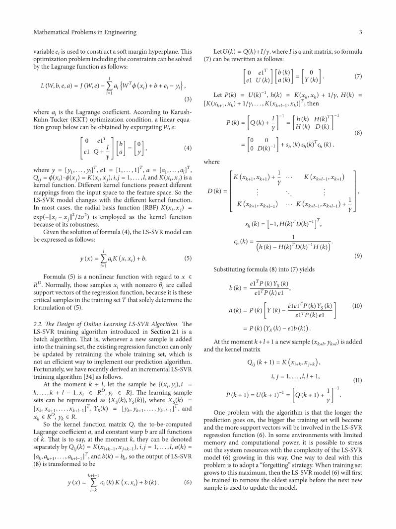
Figure 3 shows the one-step prediction results and theprediction errors when the system has no external distur-bance. The solid line means the actual output of system andthe dash line means the prediction output of our approach.According to Figure 3, the future dynamics of the system canbe predicted accurately.

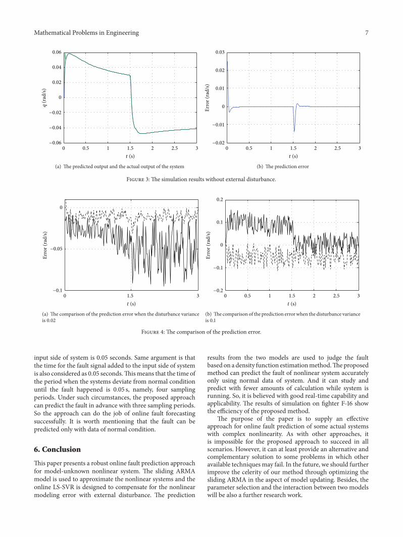
To further prove the effectiveness of the proposedmethod, the external disturbance of system is then con-sidered. In Figure 4, the prediction errors of our approachare compared with the results only with online LS-SVR.The solid line represents the errors without online LS-SVR,while the dash line represents the error of our approach.Figure 4(a) shows the result when the variance of externaldisturbance is 0.02 and Figure 4(b) shows the result whenthe variance of external disturbance is 0.1. With the varianceof external disturbance increasing, the errors of only usingonline LS-SVR are increasing rapidly, while the predictionerrors of our approach are changeless. Obviously, the pro-posed approach can compensate for the external disturbanceefficiently.

At last, the fault judgment result through hypothesis testis provided in Figure 5, when 𝑉

𝑁(𝑥) = 0.0000005. The result

shows that the fault is predicted at the time 1.5125 s when thevariance of external disturbance is 0.1, which means that thefault can be predicted in one period. As is known, the aircrafthas a flexible element in input channels to avoid the abruptchanges of control. Generally, it can be regarded as an inertialconstruction; the time to add a control completely into the


0 0.5 1 1.5 2 2.5 3

0

0.02

0.04

0.06

−0.06

−0.04

−0.02

q(r

ad/s

)

t (s)

(a) The predicted output and the actual output of the system

0 0.5 1 1.5 2 2.5 3

0

0.01

0.02

0.03

Erro

r (ra

d/s)

−0.02

−0.01

t (s)

(b) The prediction error

Figure 3: The simulation results without external disturbance.

0 1.5 3

0

Erro

r (ra

d/s)

−0.1

−0.05

t (s)

(a) The comparison of the prediction error when the disturbance varianceis 0.02

0 0.5 1 1.5 2 2.5 3

0

0.1

0.2Er

ror (

rad/

s)

−0.2

−0.1

t (s)

(b) The comparison of the prediction errorwhen the disturbance varianceis 0.1

Figure 4: The comparison of the prediction error.

input side of system is 0.05 seconds. Same argument is thatthe time for the fault signal added to the input side of systemis also considered as 0.05 seconds.Thismeans that the time ofthe period when the systems deviate from normal conditionuntil the fault happened is 0.05 s, namely, four samplingperiods. Under such circumstances, the proposed approachcan predict the fault in advance with three sampling periods.So the approach can do the job of online fault forecastingsuccessfully. It is worth mentioning that the fault can bepredicted only with data of normal condition.

6. Conclusion

This paper presents a robust online fault prediction approachfor model-unknown nonlinear system. The sliding ARMAmodel is used to approximate the nonlinear systems and theonline LS-SVR is designed to compensate for the nonlinearmodeling error with external disturbance. The prediction

results from the two models are used to judge the faultbased on a density function estimationmethod.Theproposedmethod can predict the fault of nonlinear system accuratelyonly using normal data of system. And it can study andpredict with fewer amounts of calculation while system isrunning. So, it is believed with good real-time capability andapplicability. The results of simulation on fighter F-16 showthe efficiency of the proposed method.

The purpose of the paper is to supply an effectiveapproach for online fault prediction of some actual systemswith complex nonlinearity. As with other approaches, itis impossible for the proposed approach to succeed in allscenarios. However, it can at least provide an alternative andcomplementary solution to some problems in which otheravailable techniques may fail. In the future, we should furtherimprove the celerity of our method through optimizing thesliding ARMA in the aspect of model updating. Besides, theparameter selection and the interaction between two modelswill be also a further research work.


1

0.75

0.5

0.25

00 0.5 1 1.5 2 2.5 3

t (s)

𝜃

1.5125

The h

ypot

hesis

test

ofq

Figure 5:The hypothesis test and the result of fault prediction whenthe variance of external disturbance is 0.1.

Conflict of Interests

The authors declare that there is no conflict of interestsregarding the publication of this paper.

Acknowledgments

This work is supported by Innovation Program of ShanghaiMunicipal Education Commission under Grant no. 12YZ156,the Fund of SUES under Grant no. 2012gp45, ShanghaiMunicipal Natural Science Foundation under Grant no.12ZR1412200, and National Natural Science Foundation ofChina under Grant no. 61271114.

References

[1] G. Vachtseevanos, F. Lewis, M. Roemer, A. Hess, and B. Wu,Intelligent Fault Diagnosis and Prognosis for Engineer Systems,John Wiley & Sons, 2006.

[2] S. K. Yang, “An experiment of state estimation for predictivemaintenance using Kalman filter on a DC motor,” ReliabilityEngineering and System Safety, vol. 75, no. 1, pp. 103–111, 2002.

[3] X. Hu, D. V. Prokhorov, and D. C. Wunsch II, “Time seriespredictionwith a weighted bidirectionalmulti-stream extendedKalman filter,” Neurocomputing, vol. 70, no. 13–15, pp. 2392–2399, 2007.

[4] Z. J. Zhou, C. H. Hu, H. D. Fan, and J. Li, “Fault prediction ofthe nonlinear systems with uncertainty,” Simulation ModellingPractice andTheory, vol. 16, no. 6, pp. 690–703, 2008.

[5] D. H. Zhou and P. M. Frank, “Strong tracking filtering ofnonlinear time-varying stochastic systems with coloured noise:application to parameter estimation and empirical robustnessanalysis,” International Journal of Control, vol. 65, no. 2, pp. 295–307, 1996.

[6] D. Wang, D. H. Zhou, Y. H. Jin, and S. J. Qin, “A strongtracking predictor for nonlinear processes with input timedelay,” Computers & Chemical Engineering, vol. 28, no. 12, pp.2523–2540, 2004.

[7] M. Z. Chen, D. H. Zhou, and G. P. Liu, “A new particle predictorfor fault prediction of nonlinear time-varying systems,” Devel-opments in Chemical Engineering andMineral Processing, vol. 13,no. 3-4, pp. 379–388, 2005.

[8] M. E. Orchard and G. J. Vachtsevanos, “A particle filteringapproach for on-line failure prognosis in a planetary carrierplate,” International Journal of Fuzzy Logic and IntelligentSystems, vol. 7, no. 4, pp. 221–227, 2007.

[9] X. Si, C. H. Hu, J. B. Yang, and Q. Zhang, “On the dynamicevidential reasoning algorithm for fault prediction,” ExpertSystems with Applications, vol. 38, no. 5, pp. 5061–5080, 2011.

[10] M. A. Schwabacher, “A survey of data-driven prognostics,” inProceedings of the InfoTech at Aerospace: Advancing Contempo-rary Aerospace Technologies and Their Integration, pp. 887–891,Arlington, Va, USA, September 2005.

[11] G. Niu and B. S. Yang, “Dempster-Shafer regression for multi-step-ahead time-series prediction towards data-drivenmachin-ery prognosis,” Mechanical Systems and Signal Processing, vol.23, no. 3, pp. 740–751, 2009.

[12] S. L. Ho and M. Xie, “The use of ARIMA models for reliabilityforecasting and analysis,” Computers & Industrial Engineering,vol. 35, no. 1–4, pp. 213–216, 1998.

[13] R. Y. Li and R. Kang, “Research on failure rate forecastingmethod based on ARMA model,” Systems Engineering andElectronics, vol. 30, no. 8, pp. 1588–1591, 2008.

[14] J. Zhao, L.M. Xu, and L. Lin, “Equipment fault forecasting basedon ARMA model,” in Proceedings of the IEEE InternationalConference on Mechatronics and Automation (ICMA ’07), pp.3514–3518, Harbin, China, August 2007.

[15] Z. D. Zhang and S. S. Hu, “Fault prediction of fighter based onnonparametric density estimation,” Journal of Systems Engineer-ing and Electronics, vol. 16, no. 4, pp. 831–836, 2005.

[16] J. T. Connor, R. D. Martin, and L. E. Atlas, “Recurrent neuralnetworks and robust time series prediction,” IEEE Transactionson Neural Networks, vol. 5, no. 2, pp. 240–254, 1994.

[17] S. L. Ho, M. Xie, and T. N. Goh, “A comparative study ofneural network and box-jenkins ARIMA modeling in timeseries prediction,” Computers & Industrial Engineering, vol. 42,no. 2–4, pp. 371–375, 2002.

[18] G. Xue, L. Xiao, M. Bie, and S. Lu, “Fault prediction ofboilers with fuzzy mathematics and RBF neural network,” inProceedings of the International Conference on Communications,Circuits and Systems, vol. 2, pp. 1012–1016, Hong Kong, May2005.

[19] M. Luo, D. Wang, M. Pham et al., “Model-based fault diag-nosis/prognosis for wheeled mobile robots: a review,” in Pro-ceedings of the 31st Annual Conference of IEEE IndustrialElectronics Society (IECON ’05), pp. 2267–2272, Raleigh, NC,USA, November 2005.

[20] C. H. Hu, X. P. Cao, and W. Zhang, “Fault prediction based onBayesian MLP neural networks,” GESTS Transaction Journal,vol. 16, no. 1, pp. 17–25, 2005.

[21] G. Yang and X. Wu, “Fault prediction of ship machinery basedon gray neural network model,” in Proceedings of the IEEEInternational Conference on Control and Automation (ICCA’07), pp. 1063–1066, Guangzhou, China, June 2007.

[22] H. G. Han and J. F. Qiao, “Prediction of activated sludge bulkingbased on a self-organizing RBF neural network,” Journal ofProcess Control, vol. 22, no. 6, pp. 1103–1112, 2012.

[23] D. Basllk, S. Pal, and D. C. Patranabis, “Support vector regres-sion,” Neural Information Processing—Letters and Reviews, vol.11, no. 10, pp. 203–224, 2003.

[24] U.Thissena and R. Brakela, “Using support vector machines fortime series prediction,” Chemometrics & Intelligent LaboratorySystems, vol. 6, pp. 35–49, 2003.


[25] A. J. Smola and B. Scholkopf, “A tutorial on support vectorregression,” Statistics and Computing, vol. 14, no. 3, pp. 199–222,2004.

[26] X. X. Ma, X. Y. Huang, and Y. Chai, “Fault process trendprediction based on support vector machines,” Acta SimulataSystematica Sinica, vol. 14, pp. 1548–1551, 2002.

[27] K. Y. Chen, “Forecasting systems reliability based on supportvector regression with genetic algorithms,” Reliability Engineer-ing and System Safety, vol. 92, no. 4, pp. 423–432, 2007.

[28] S. Hou and Y. Li, “Short-term fault prediction based on supportvector machines with parameter optimization by evolutionstrategy,” Expert Systems with Applications, vol. 36, no. 10, pp.12383–12391, 2009.

[29] D. T. Liu, Y. Peng, and X. Y. Peng, “Online adaptive statusprediction strategy for data-driven fault prognostics of complexsystems,” inProceedings of the Prognostics& SystemHealthMan-agement Conference (PHM-Shenzhen ’11), pp. 1–6, Shenzhen,China, May 2011.

[30] L. Ye, D. H. You, X. G. Yin, K.Wang, and J. C.Wu, “An improvedfault-location method for distribution system using waveletsand support vector regression,” Electrical Power and EnergySystems, vol. 55, pp. 467–472, 2014.

[31] A. Baylar, D. Hanbay, and M. Batan, “Application of leastsquare support vector machines in the prediction of aerationperformance of plunging overfall jets from weirs,” ExpertSystems with Applications, vol. 36, no. 4, pp. 8368–8374, 2009.

[32] Y. H. Gao and Y. B. Li, “Fault prediction model based onphase space reconstruction and least squares support vectormachines,” in Proceeding of the 9th International Conference onHybrid Intelligent Systems (HIS '09), pp. 464–467, Shenyang,China, August 2009.

[33] J. A. K. Suykens, J. De Brabanter, L. Lukas, and J. Vandewalle,“Weighted least squares support vector machines: robustnessand sparce approximation,” Neurocomputing, vol. 48, pp. 85–105, 2002.

[34] S. Su andW. Zhang, “Fault prediction of nonlinear system usingtime series novelty estimation,” Journal of Digital InformationManagement, vol. 11, no. 3, pp. 207–212, 2013.

[35] J. Q. Fan and Q. W. Yao, Nonlinear Time Series: Nonparametricand Parametric Methods, pp. 12–123, Springer, New York, NY,USA, 2003.

[36] Y. Liu, Intelligent Adaptive Reconfigurable Control for ComplexNonlinear System, NanjingUniversity of Aeronautics andAstro-nautics, Nanjing, China, 2003.

Submit your manuscripts athttp://www.hindawi.com

Hindawi Publishing Corporationhttp://www.hindawi.com Volume 2014

MathematicsJournal of


Mathematical Problems in Engineering

Hindawi Publishing Corporationhttp://www.hindawi.com

Differential EquationsInternational Journal of

Volume 2014

Applied MathematicsJournal of


Probability and StatisticsHindawi Publishing Corporationhttp://www.hindawi.com Volume 2014

Journal of


Mathematical PhysicsAdvances in

Complex AnalysisJournal of


OptimizationJournal of


CombinatoricsHindawi Publishing Corporationhttp://www.hindawi.com Volume 2014

International Journal of


Operations ResearchAdvances in

Journal of


Function Spaces

Abstract and Applied AnalysisHindawi Publishing Corporationhttp://www.hindawi.com Volume 2014

International Journal of Mathematics and Mathematical Sciences


The Scientific World JournalHindawi Publishing Corporation http://www.hindawi.com Volume 2014


Algebra

Discrete Dynamics in Nature and Society



Decision SciencesAdvances in

Discrete MathematicsJournal of

Hindawi Publishing Corporationhttp://www.hindawi.com

Volume 2014 Hindawi Publishing Corporationhttp://www.hindawi.com Volume 2014

Stochastic AnalysisInternational Journal of

research article fault prediction for nonlinear system...

Documents