Closed-Form Prediction of Nonlinear Dynamic Systems by Means ofGaussian Mixture Approximation of the Transition Density

Marco Huber, Dietrich Brunn, and Uwe D. Hanebeck

Abstract— Recursive prediction of the state of a nonlinearstochastic dynamic system cannot be efficiently performedin general, since the complexity of the probability densityfunction characterizing the system state increases with everyprediction step. Thus, representing the density in an exactclosed-form manner is too complex or even impossible. So, anappropriate approximation of the density is required. Insteadof directly approximating the predicted density, we propose theapproximation of the transition density by means of Gaussianmixtures. We treat the approximation task as an optimizationproblem that is solved offline via progressive processing tobypass initialization problems and to achieve high qualityapproximations. Once having calculated the transition densityapproximation offline, prediction can be performed efficientlyresulting in a closed-form density representation with constantcomplexity.

I. INTRODUCTION

Estimation of uncertain quantities is a typical challenge inmany engineering applications like information processing insensor-actuator-networks, localization of vehicles or roboticsand machine learning. One aspect that arises is the inferenceof a given uncertain quantity through time. Particularly therecursive processing of this so-called prediction requires anefficient implementation for practical applications.

Typically, random variables are used to describe the quan-tities and their uncertainties. For such a representation theprediction problem is solved by the Bayesian estimator. Ingeneral, the probability density of the predicted quantitycannot be calculated in closed form and the complexity ofthe density representation increases with each time step. Theconsequence of this is an impractical computational effort.Only for some special cases full analytical solutions areavailable. For linear systems with Gaussian random variablesthe Kalman filter provides exact solutions in an efficientmanner [7]. Versatile approximative techniques exist for thecase of nonlinear systems: To overcome the problem ofrepresenting the whole predicted density, particle filters usesamples instead [2]. They are easy to implement and toparallelise, but it is still a hard task to obtain adequatesamples at every prediction step. Another possibility arisesfrom the usage of generic parameterized density functions.The well known extended Kalman filter uses linearization toapply the Kalman filter equations on nonlinear systems [10],while the unscented Kalman filter offers in addition higherorder accuracy by using a deterministic sampling approach[6]. The resulting single Gaussian density of both estimation

Marco Huber, Dietrich Brunn, and Uwe D. Hanebeck are with the Intel-ligent Sensor-Actuator-Systems Laboratory, Institute of Computer Scienceand Engineering, Universitat Karlsruhe (TH), Germany.mhuber|brunn@ira.uka.de, uwe.hanebeck@ieee.org

methods is typically not a sufficient representation for thetrue complex density. Due to their universal approximationproperty, Gaussian mixtures [8] are a much better approachfor parameterized density functions. The bandwidth of esti-mators using Gaussian mixtures is wide. It ranges from theefficient Gaussian sum filter [1] that allows only an individualupdating of the mixture components up to computationallymore expensive but precise methods [5].

In this paper, we introduce a new closed-form predictionapproach for nonlinear systems by means of a Gaussian mix-ture approximation of the transition density. The transitiondensity is used to propagate the probability density of thecurrent system state to the next time step. By approximatingit, the prediction step can be solved analytically and results ina Gaussian mixture representation of the predicted density.To avoid getting trapped in local optima, and thus ensurea high accuracy, we approximate the transition density in aprogressive way. For that purpose, a parameterized transitiondensity is introduced, which starts from a simple densityand continuously approaches the true transition density. Thenecessary demanding computations can be calculated offline,whereas the prediction still remains an online task, thatis reduced to simple multiplications of Gaussian densities.Hence, an efficient prediction is available.

In the following section, we will review the Bayesianestimator for discrete-time systems and point out the relationbetween transition density and system model. Furthermore,the requirements for offline approximation are formulated.The rest of the paper is structured as follows: Section IIIderives the closed-form prediction of nonlinear systems usinga special case of Gaussian mixtures for transition densityapproximation. The actual approximation and its progres-sive processing is explained in Section IV together withan example application comprising a cubic system model.Section V further investigates the cubic system model inorder to compare and discuss the results of the new predictionapproach with those of the extended Kalman filter and theBayesian estimator. The paper closes with a conclusion andan outlook to future work.

II. PROBLEM FORMULATION

For the sake of brevity and clarity, we only considerscalar random variables, denoted by boldface letters, e.g. x.Furthermore, we regard nonlinear, time-invariant, discrete-time systems with a system equation

xk+1 = a(xk) + wk , (1)

where xk is the scalar system state at time step k andwk is additive noise representing the unknown disturbanceacting upon the system. It is assumed as a white, stationaryGaussian random process with density fw(wk) = N (wk −µw, σw), where µw is the mean and σw is the standarddeviation.

To simplify matters, we just consider the state evolutionin abscence of a system input as in (1). All results of thispaper also hold in the presence of a non-zero system input.

While dealing with the measurement or filter step depend-ing on the measurement equation is subject of future work,we focus in this paper on the system equation (1). Given anestimate fx

0 (x0) for x0 at k = 0, this equation is used in aBayesian setting for a recursive system state propagation intime. According to [11] this so-called prediction step of theBayesian estimator results in a density

fxk+1(xk+1) =

∫R

fT (xk+1)fxk (xk)dxk (2)

for xk+1, where fT (xk+1) is the transition density

fT (xk+1) = f(xk+1|xk) = fw(xk+1 − a(xk)) ,

which depends upon the noise density of wk and the struc-ture of the system equation. Since (1) is time-invariant andwk is stationary, this bivariate density is also time-invariant,i.e., its shape is constant for all time steps k.

In general, the recursive Bayesian estimator is computa-tionally impractical. The complex shape of the transitiondensity fT (xk+1) prevents a closed-form and above allan efficient solution of (2). In general, no exact analyticaldensity can be generated in the prediction step. Hence,for the general case of nonlinear systems with arbitrarydistributed random variables an approximation of the truepredicted density is inevitable. From now on true densitieswill be denoted by a tilde, e.g. f(·), while the correspondingapproximation will be denoted by f(·).

Since directly approximating the true predicted densityfx

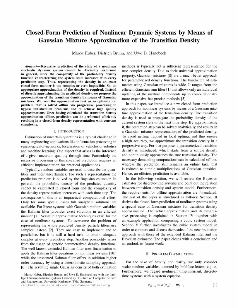
k+1(xk+1) is difficult, we use a Gaussian mixture represen-tation fT(xk+1, η) of fT(xk+1) for approximation purposes1,that depends upon the parameter vector η. For high qualityapproximations, an appropriate parameter vector η has tobe calculated, that minimizes a given distance measureG(η) between the true transition density fT(xk+1) and itsapproximation fT(xk+1, η). This resulting optimization taskcan be solved offline and independent of the prediction asshown in Figure 1. For this we take advantage of the factthat in real systems the system state is usually restricted toa finite interval, i.e.,

∀k : xk ∈ [a, b] =: Ω . (3)

So, we are only interested in approximating the transitiondensity for xk ∈ Ω. Together with the property of time-invariance of fT(xk+1), offline approximation is possible.Section IV explains the approximation in detail.

1The reader is reminded that fT(xk+1) and fT(xk+1, η) should alwaysbe regarded as functions of (xk, xk+1).

fxk+1(xk+1)

fx0 (x0)

fxk (xk)

a(·) fw(wk)

ApproximateTransition Density

UnitDelay

fT(x

k+

1,η

)

offlineonline

Closed-formPrediction Step

Fig. 1. Recursive, closed-form prediction. The necessary transition densityapproximation is performed offline, before the prediction. That one remainsan online task.

III. THE PREDICTION STEP

The transition density approximation allows to performan efficient, closed-form prediction step online, depictedin Figure 1. For this purpose we assume that all involveddensities are represented as Gaussian mixtures.

First we assume fxk (xk) is given by

fxk (xk) =

Lk∑j=1

wxk,jN (xk − µx

k,j , σxk,j) , (4)

where Lk is the number of Gaussian components, N (xk −µx

k,j , σxk,j) is a Gaussian density with mean µx

k,j and standarddeviation σx

k,j and wxk,j are weighting coefficients with

wxk,j > 0 and

∑Lk

j=1 wxk,j = 1.

For the given Gaussian mixture approximationfT(xk+1, η) we use the special case of a Gaussianmixture with axis-aligned Gaussian components (short:axis-aligned Gaussian mixture). Here, every component isseparable in each dimension according to

fT(xk+1, η) =LT∑i=1

wiN (xk − µ1i , σ

1i )N (xk+1 − µ2

i , σ2i ) ,

(5)

with the parameter vector

η = [ηT1, ηT

2, . . . , ηT

LT]T

where

ηi= [wi, µ

1i , σ

1i , µ2

i , σ2i ]

T.

Such a representation of fT(xk+1, η) is very convenient forefficiently performing the prediction step.

Theorem 1 (Approximate Predicted Density)Given the Gaussian mixture representations (4) and (5)for fx

k (xk) and fT(xk+1, η) respectively, the approximatepredicted density fx

k+1(xk+1) is also a Gaussian mixturewith LT components that can be calculated analytically.

PROOF. Using the Bayesian prediction equation (2) we obtain

fxk+1(xk+1) =

ZR

fT(xk+1, η)fxk (xk)dxk

=

LTXi=1

wiN (xk+1 − µ2i , σ

2i )

LkXj=1

wxk,j

ZR

N (xk − µ1i , σ

1i )N (xk − µx

k,j , σxk,j)dxk| z

=:zi,j (constant)

!

=

LTXi=1

wk+1,iN (xk+1 − µ2i , σ

2i ) (6)

with wk+1,i = wi

PLkj=1 wx

k,jzi,j .The number of components in fx

k+1(xk+1) depends only on thenumber of components in fT(xk+1, η). Thus, the complexity offx

k+1(xk+1) remains constant over time.For getting the result in (6), only the integral over a

multiplication of two Gaussian densities, denoted as zi,j , has tobe solved. This corresponds exactly to the prediction step of aKalman filter. Hence, (6) provides the closed-form and efficientsolution for the prediction step by means of the Gaussian mixtureapproximation of a transition density.

Generally, the more components fT(xk+1, η) contains, themore accurate the approximation of fx

k+1(xk+1) is. Using anon axis-aligned Gaussian mixture for fT(xk+1, η) insteadan exponential growth of components for fx

k+1(xk+1) wouldbe the consequence.

The two following remarks give attention to some conse-quences of Theorem 1.

Remark 1 (Gaussian Mixture Reduction) Several estima-tors using Gaussian mixture density representations sufferfrom the exponential growth of components. Theorem 1 offersa simple method for Gaussian mixture component reductionby applying additional prediction steps with the transitiondensity approximation of the linear system

xk+1 = xk + wk .

To keep the introduced error small, wk is Gaussian withzero-mean and standard deviation 0 < σw 1.

Remark 2 (Normalization) Typically fxk+1(xk+1) is not a

valid probability density function, because∑LT

i=1 wk+1,i 6= 1.This originates from the fact, that fT(xk+1, η) is just an ap-proximation of the true transition density. To achieve a validprobability density for fx

k+1(xk+1) we have to normalize itby multiplication with 1PLT

i=1 wk+1,i

.

IV. APPROXIMATION OF THE TRANSITION DENSITY

The quality of the approximation fxk+1(xk+1) strongly

depends on the similarity between fT(xk+1) and its Gaussianmixture approximation fT(xk+1, η) for xk ∈ Ω. So, thissection is concerned with solving the optimization problem

ηmin

= arg minη

G(η) , (7)

Init. Progression: γ = 0

Result: fT (xk+1, η) γ ≤ 1

Increment: γ = γ + ∆γ

Optimize current Progression Stepby minimizing G(η, γ)

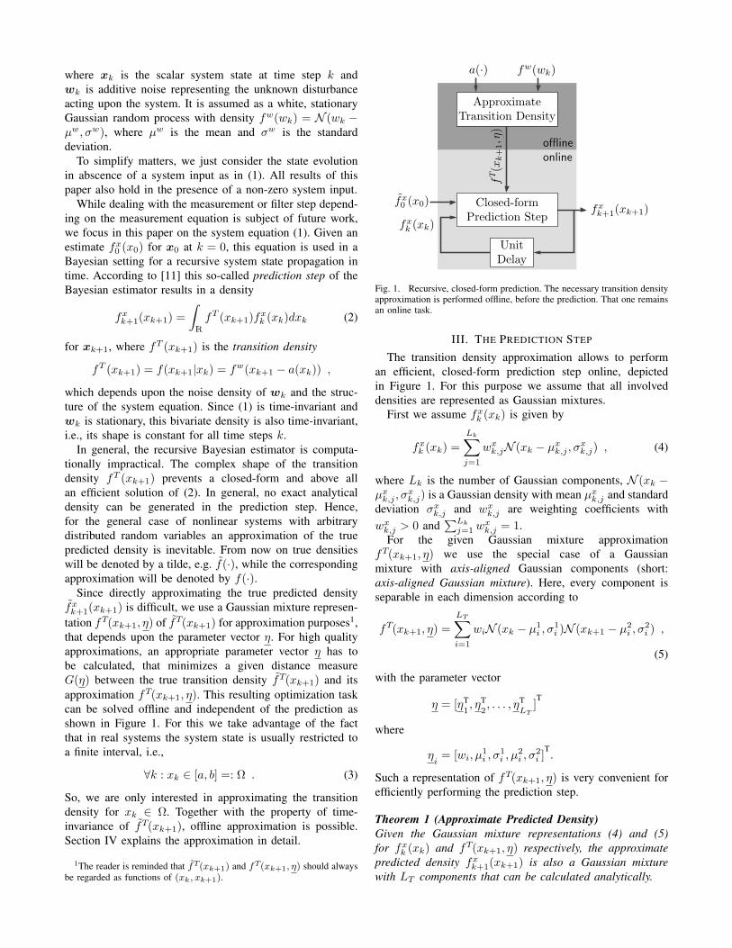
Fig. 2. Flow chart of the progressive processing of ηmin

.

that yields the parameter vector for fT(xk+1, η) minimizingthe distance to fT(xk+1). As distance measure we take thesquared integral measure

G(η) =12

∫R

∫R

(fT(xk+1)− fT(xk+1, η)

)2

dxkdxk+1 . (8)

Although this measure has been selected for its simplicityand convenience, it has been found to give excellent perfor-mance. Of course, the methods of this paper are not restrictedto this measure.

Independent of the selected distance measure, Gaussianmixture approximations are considered a tough problem. Ingeneral, no closed-form solution of (7) can be derived. Inaddition, the high dimension of η complicates the selection ofan initial solution, so that the direct application of numericalminimization routines causes insufficient local optima for η.

A. Approximation by Means of Progressive Processing

Instead of attempting to directly approximate the transitiondensity, we pursue a progressive approach for finding η

minas

shown in Figure 2. This type of processing has been proposedin [5], [9]. In doing so, a parameterized transition densityfT(xk+1, γ) with the progression parameter γ ∈ [0, 1] isintroduced. This progression parameter ensures a continuoustransformation of the solution of an initial, tractable opti-mization problem towards the desired true transition densityfT(xk+1) by tracking a gradually changing distance measureG(η, γ).

For γ = 0 the initial optimization consists of approximat-ing the transition density of the linear system

xk+1 = A · xk + wk , (9)

where A ∈ R. As discussed in Section IV-E, this prob-lem easily allows calculating an optimum by numericalopimization without an initial parameter selection by theuser. Starting from this optimum the progression parameterγ is gradually incremented by ∆γ. In every single so-calledprogression step the distance measure G(η, γ) between theparameterized transition density fT(xk+1, γ) and its approxi-mation fT(xk+1, η) is minimized by employing of the BFGSformula [3], a well known optimization method.

The approximation fT(xk+1, η), or more precisely theparameter vector η, follows gradually fT(xk+1, γ) until the

desired true transition density fT(xk+1) is finally reachedfor γ = 1. Hence, for fT(xk+1, γ) we obtain

fT (xk+1, γ = 0) = fw(xk+1 −A · xk) ,

fT (xk+1, γ = 1) = fT(xk+1) ,(10)

if xk ∈ Ω, otherwise

fT(xk+1, γ) = 0 .

This progressive processing of (7) bypasses the choice ofinsufficient starting parameters. Hence, the typical problemof obtaining suboptimal solutions is attenuated or evenprevented with a proper choice of ∆γ.

B. Parameterized System FunctionTo introduce the parameterized transition density, we use

the parameterized system function a(xk, γ)

a(xk, γ) = (1− γ)A · xk + γa(xk) ,

where in particular

a(xk, γ = 0) = A · xk ,

a(xk, γ = 1) = a(xk) .

This yields the modified system equation

xk+1 = a(xk, γ) + wk . (11)

The dependence of fT(xk+1, γ) = fw(xk+1 − a(xk, γ)) onsystem equation (11) automatically causes its parameteriza-tion according to (10).

Example 1 (Cubic System Function) Considering the sys-tem equation xk+1 = a(xk)+wk with a(xk) = 2xk−0.5x3

k, thecorrespondig parameterized system function is a(xk, γ) = (1−γ)A ·xk + γ(2xk − 0.5x3

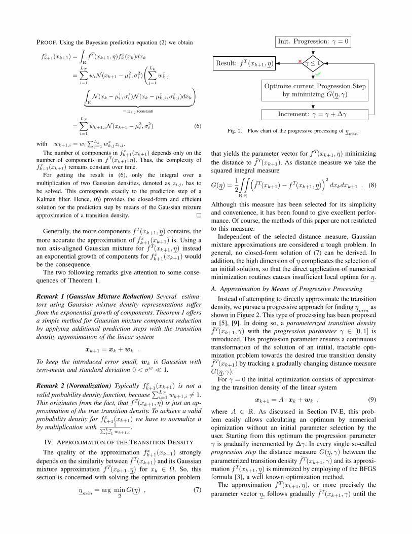
k). Figure 3(a) shows the progressionfor ∆γ = 0.2, A = 0 and Ω = [−3, 3]. The parameterized tran-sition density fT(xk+1, γ) performs the same transformation.

C. Axis-Aligned Gaussian Mixture ApproximationUsing axis-aligned Gaussian mixtures for approximating

fT(xk+1) is also advantageous for optimization purposes.An axis-aligned Gaussian mixture has minor approximationcapabilities compared to a non axis-aligned one. Hence,more components are needed to achieve a comparable ap-proximation quality. In exchange, the covariance matrixof axis-aligned Gaussian mixtures is diagonal. Thus, lessparameters for a single component have to be adjusted andthe necessary determination of the gradient ∂G

∂η prove to beeasier. Altogether, representing fT(xk+1, η) as in (5) lowersthe algorithmic complexity.

During the progression it is possible that the weights wi

of fT(xk+1, η) become negative. To ensure a valid densityfunction, we use quadratic weights instead. Henceforth, wewrite in difference to (5)

fT(xk+1, η) =LT∑i=1

w2iN (xk − µ1

i , σ1i )N (xk+1 − µ2

i , σ2i ) ,

without affecting the result of the prediction in principle. Itmust be pointed out that the probability mass of fT(xk+1)is not equal to 1, as it is a conditional density.

D. Squared Integral Distance MeasureThe goal of the progression is to calculate the parameters

η minimizing G(η). Thus, we use also the squared integraldistance measure for G(η, γ) by plugging the progressiveversion fT(xk+1, γ) of fT(xk+1) in (8). Converting (8) andconsidering (10) results in

G(η, γ) =12

∫R

∫Ω

(fT(xk+1, γ)

)2

dxkdxk+1

−∫R

∫Ω

fT(xk+1, γ)fT(xk+1, η)dxkdxk+1

︸ ︷︷ ︸=:I

+12

∫R

∫R

(fT(xk+1, η)

)2dxkdxk+1 , (12)

where merely the integral I cannot be solved analytically.Numerical integration methods like the adaptive Simpsonquadrature [4] have to be applied.

The necessary condition for the existence of a minimumof G(η, γ) for a given γ is

∂G(η, γ)∂η

= 0 . (13)

Since (13) allows no closed-form solution we use the BFGSformula for minimization, which depends on calculating thegradient

∂G(η,γ)

∂η . To obtain the gradient it is sufficient to ex-amine only the i-th component fT

i (xk+1, ηi) of fT(xk+1, η)

∂G(η, γ)∂η

i

=−∫R

∫Ω

fT(xk+1, γ)∂fT

i (xk+1, ηi)

∂ηi

dxkdxk+1

+∫R

∫R

fT(xk+1, η)∂fT

i (xk+1, ηi)

∂ηi

dxkdxk+1 ,

with

fTi (xk+1,ηi

) = w2iN (xk − µ1

i , σ1i )N (xk+1 − µ2

i , σ2i ) .

Stacking all i = 1, . . . , LT partial derivatives leads to∂G(η,γ)

∂η . Evaluating the gradient requires also numericalintegration.

E. InitializationA complete analytical solution of (12) is given for γ = 0.

Here, the parameterized transition density

fT (xk+1, γ = 0) = fw(xk+1 −A · xk)= N (xk+1 −A · xk − µw, σw)

depends on the linear system equation (9). We can takeadvantage of the linearity as we initialize the progression byavoiding the selection of initial parameters η for fT(xk+1, η)by the user. For this, fixed and equidistant means for thecomponents of fT(xk+1, η) are given by

µ1i = a + i · b− a

LT + 1,

µ2i = A · µ1

i + µw .

−3 −2 −1 0 1 2 3−8

−6

−4

−2

0

2

4

6

8

xk →

xk+

1→

γ = 0γ = 0.2γ = 0.4γ = 0.6γ = 0.8γ = 1

(a) (b)−3 −2 −1 0 1 2 3

−8

−6

−4

−2

0

2

4

6

8

xk →

xk+

1→

(c)

Fig. 3. (a) Progression of the parameterized system function a(xk, γ) = (1− γ)A ·xk + γ(2xk − 0.5x3k). (b) Approximation of the transition density

fT(xk+1) = N`xk+1 − (2xk − 0.5x3

k), 1´

with quality G(η) = 0.0067. (c) Covariance ellipses of the components for γ = 0 (gray) and γ = 1 (black).

Thus, only the weighting coefficients wi and the standard de-viations σ1

i , σ2i are adjustable. A further parameter reduction

occurs by taking the same weights and standard deviationsfor all components. As a result, there are just the threeparameters

wi = w, σ1i = σ1, σ2

i = σ2

that have to be optimized. This optimization problem has onesingle global optimum. So, no user initialization is requiredand as a consequence the risk of starting the progression withan insufficient local optimum is obviously avoided.

Example 2 (Cubic System Function (cont’d.)) We consideragain the cubic system equation of Example 1, now withsystem noise wk = N (wk − 0, 1) and Ω = [−3, 3]. Usingthe parameterized system function of Example 1 with A = 0and a Gaussian mixture with LT = 20 components leads tothe transition density approximation shown in Figure 3(b). Fig-ure 3(c) depicts the covariance ellipses of the single Gaussiancomponents at the beginning and the end of the progression.

F. Generalization

Until now we assumed, that the system noise wk isGaussian. All the derivations of this paper can be directlygeneralized to noise that is represented by a Gaussian mix-ture. For general densities of wk it is possible to first finda Gaussian mixture approximation of fw(wk) and then toapproximate the transition density afterwards.

V. EXAMPLE: PREDICTION

In this section we investigate the prediction results for thesystem equation

xk+1 = 2xk − 0.5x3k + wk ,

introduced in Examples 1 and 2. The system noise wk iswhite Gaussian with density fw = N (wk − µw, σw), where

µw = 0 and σw = 0.175. We approximate the transitiondensity of this system according to Example 2 for xk ∈ Ω =[−3, 3], but now with LT = 50 Gaussian components forfT(xk+1, η) since the standard deviation σw is now muchsmaller. This results in a quality G(η) = 0.0207.

Starting with the density

fx0 (x0) = N (x0 − 0.4, 0.8)

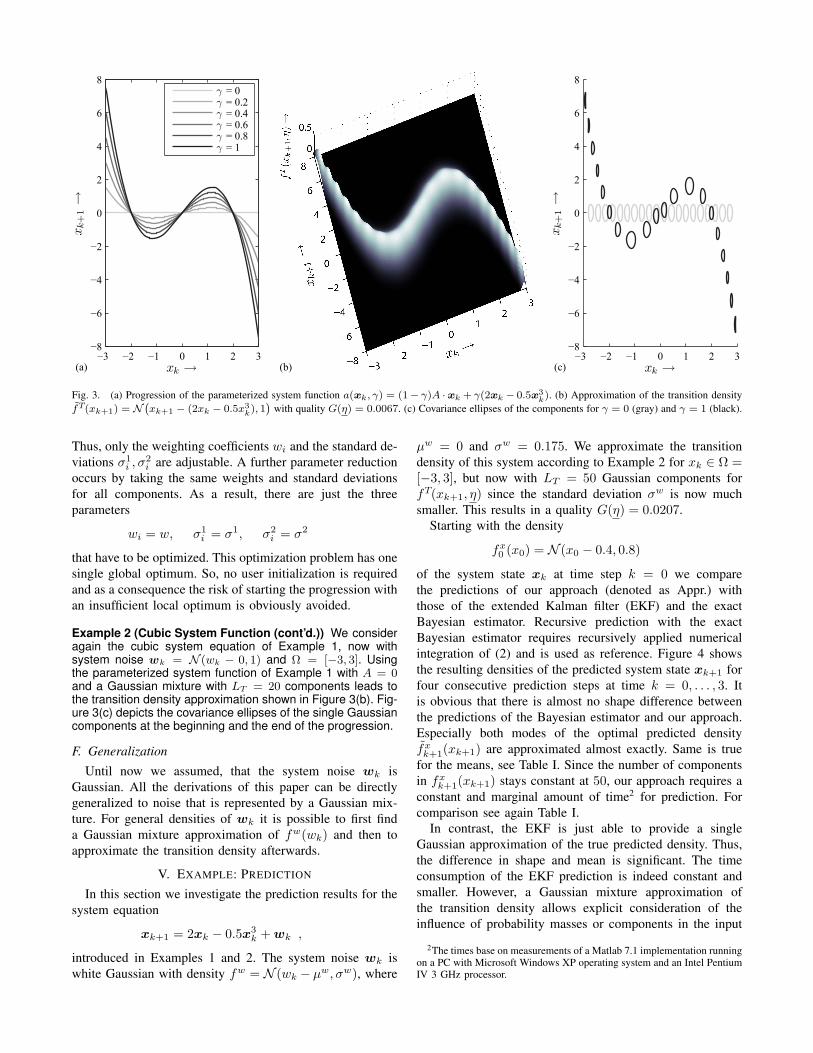
of the system state xk at time step k = 0 we comparethe predictions of our approach (denoted as Appr.) withthose of the extended Kalman filter (EKF) and the exactBayesian estimator. Recursive prediction with the exactBayesian estimator requires recursively applied numericalintegration of (2) and is used as reference. Figure 4 showsthe resulting densities of the predicted system state xk+1 forfour consecutive prediction steps at time k = 0, . . . , 3. Itis obvious that there is almost no shape difference betweenthe predictions of the Bayesian estimator and our approach.Especially both modes of the optimal predicted densityfx

k+1(xk+1) are approximated almost exactly. Same is truefor the means, see Table I. Since the number of componentsin fx

k+1(xk+1) stays constant at 50, our approach requires aconstant and marginal amount of time2 for prediction. Forcomparison see again Table I.

In contrast, the EKF is just able to provide a singleGaussian approximation of the true predicted density. Thus,the difference in shape and mean is significant. The timeconsumption of the EKF prediction is indeed constant andsmaller. However, a Gaussian mixture approximation ofthe transition density allows explicit consideration of theinfluence of probability masses or components in the input

2The times base on measurements of a Matlab 7.1 implementation runningon a PC with Microsoft Windows XP operating system and an Intel PentiumIV 3 GHz processor.

−2 0 20

0.5

1

1.5k = 0

xk+1 →

fx k+

1(x

k+

1)→

−2 0 20

0.5

1

1.5k = 0

xk+1 →

fx k+

1(x

k+

1)→

−2 0 20

0.5

1

1.5k = 1

xk+1 →

fx k+

1(x

k+

1)→

−2 0 20

0.5

1

1.5k = 1

xk+1 →

fx k+

1(x

k+

1)→

−2 0 20

0.5

1

1.5k = 2

xk+1 →

fx k+

1(x

k+

1)→

−2 0 20

0.5

1

1.5k = 2

xk+1 →

fx k+

1(x

k+

1)→

−2 0 20

0.5

1

1.5k = 3

xk+1 →

fx k+

1(x

k+

1)→

−2 0 20

0.5

1

1.5k = 3

xk+1 →

fx k+

1(x

k+

1)→

EKFBayes

Appr.Bayes

Fig. 4. The upper plots show the predicted densities using the approach of this paper (red, solid) and the Bayesian estimator (blue, dashed). The predictionsof the Bayesian estimator in comparison with those of the extended Kalman filter (red, solid) are depicted on the lower plots.

TABLE IMEANS OF THE PREDICTED DENSITIES AND THE PREDICTION TIME.

mean: µxk+1 time: t/s

k Bayes Appr. EKF Bayes Appr. EKF0 0.404 0.408 0.768 6.016 0.166 0.0031 0.447 0.454 1.31 223.8 0.172 0.0052 0.453 0.462 1.496 14040 0.125 0.0063 0.454 0.465 1.318 6·105 0.125 0.002

density to the predicted density, by affecting the update of theweights wk+1,i of fx

k+1(xk+1) according to (6). So, higherapproximation accuracy is available and enhanced with anincreasing number of components LT .

VI. CONCLUSIONS AND FUTURE WORK

This paper introduced a novel approach for closed-formprediction of dynamic time-invariant nonlinear systems basedon approximate transition densities. Approximating transitiondensities by means of Gaussian mixtures with axis-alignedcomponents leads to an optimization problem. As most ofthe optimization methods suffer from getting trapped in localoptima, a progressive processing is proposed that transformsthe solution of an initial, tractable optimization problemcontinuously towards the desired transition density. As aresult, high quality approximations are obtained. Since theoptimization problem is solved offline, great effort can bespent without restricting the efficiency of the prediction step.

Due to the Gaussian mixture representation of the transi-tion density, the prediction result is calculated analytically.Using axis-aligned Gaussian mixtures leads to a constantnumber of components describing the approximation of thepredicted density. Thus, we obtain an efficient recursive pre-diction, whose accuracy depends on the adjustable transitiondensity approximation. These properties were demonstratedby recursively predicting the system state of a cubic system.

The described approach has been introduced for scalarrandom variables for the sake of brevity and clarity. It

can be generalized to random vectors in a straightforwardmanner. Considering the filter step is also part of futurework. Generally, the progressive processing offers room forimprovement. For example, an adaptive progression param-eter increment and adjustment of the number of Gaussianmixture components during the progression for additionalapproximation quality enhancement are possible.

VII. ACKNOWLEDGEMENTS

This work was partially supported by the GermanResearch Foundation (DFG) within the Research Train-ing Group GRK 1194 “Self-organizing Sensor-Actuator-Networks”.

REFERENCES

[1] D. L. Alspach and H. W. Sorenson, “Nonlinear Bayesian Estimationusing Gaussian Sum Approximation,” IEEE Transactions on AutomaticControl, vol. 17, no. 4, pp. 439–448, August 1972.

[2] A. Doucet, N. de Freitas, and N. Gordon, Eds., Sequential Monte CarloMethods in Practice, ser. Statistics for Engineering and InformationScience. Springer-Verlag, 2001.

[3] R. Fletcher, Practical Methods of Optimization, 2nd ed. John Wileyand Sons Ltd, 2000.

[4] W. Gander and W. Gautschi, “Adaptive Quadrature - Revisited,” BIT,vol. 40, no. 1, March 2000.

[5] U. D. Hanebeck, K. Briechle, and A. Rauh, “Progressive Bayes: ANew Framework for Nonlinear State Estimation,” in Proceedings ofSPIE, vol. 5099. AeroSense Symposium, 2003.

[6] S. J. Julier and J. K. Uhlmann, “Unscented Filtering and NonlinearEstimation,” in Proceedings of the IEEE, vol. 92, no. 3, 2004.

[7] R. E. Kalman, “A new Approach to Linear Filtering and PredictionProblems,” Transactions of the ASME, Journal of Basic Engineering,no. 82, pp. 35–45, 1960.

[8] V. Maz’ya and G. Schmidt, “On approximate approximations usingGaussian kernels,” IMA Journal of Numerical Analysis, vol. 16, no. 1,pp. 13–29, 1996.

[9] N. Oudjane and C. Musso, “Progressive Correction for RegularizedParticle Filters,” in Proceedings of the 3rd International Conferenceon Information Fusion, 2000.

[10] A. Papoulis, Probability, Random Variables and Stochastic Processes,3rd ed. McGraw-Hill, 1991.

[11] F. C. Schweppe, Uncertain Dynamic Systems. Prentice-Hall, 1973.