online service with delay - duke computer sciencedebmalya/papers/stoc17-osd.pdf · online service...

Online Service with DelayYossi Azar

Blavatnik School of Computer Science

Tel Aviv University

Israel

[email protected]

Arun Ganesh

Department of Computer Science

Duke University

USA

[email protected]

Rong Ge


Duke University

USA

[email protected]

Debmalya Panigrahi


Duke University

USA

[email protected]

ABSTRACTIn this paper, we introduce the online service with delay problem.

In this problem, there are n points in a metric space that issue ser-

vice requests over time, and a server that serves these requests.

The goal is to minimize the sum of distance traveled by the server

and the total delay (or a penalty function thereof) in serving the

requests. This problem models the fundamental tradeo between

batching requests to improve locality and reducing delay to improve

response time, that has many applications in operations manage-

ment, operating systems, logistics, supply chain management, and

scheduling.

Our main result is to show a poly-logarithmic competitive ratio

for the online service with delay problem. This result is obtained

by an algorithm that we call the preemptive service algorithm. The

salient feature of this algorithm is a process called preemptive ser-

vice, which uses a novel combination of (recursive) time forwarding

and spatial exploration on a metric space. We also generalize our

results to k > 1 servers, and obtain stronger results for special met-

rics such as uniform and star metrics that correspond to (weighted)

paging problems.

CCS CONCEPTS• Theory of computation → Online algorithms;

KEYWORDSPaging, weighted paging, k-server, online algorithms, competitive

ratio.

ACM Reference format:Yossi Azar, Arun Ganesh, Rong Ge, and Debmalya Panigrahi. 2017. Online

Service with Delay. In Proceedings of 49th Annual ACM SIGACT Symposiumon the Theory of Computing, Montreal, Canada, June 2017 (STOC’17), 13 pages.

DOI: 10.1145/3055399.3055475

Permission to make digital or hard copies of all or part of this work for personal or

classroom use is granted without fee provided that copies are not made or distributed

for prot or commercial advantage and that copies bear this notice and the full citation

on the rst page. Copyrights for components of this work owned by others than ACM

must be honored. Abstracting with credit is permitted. To copy otherwise, or republish,

to post on servers or to redistribute to lists, requires prior specic permission and/or a

fee. Request permissions from [email protected].

STOC’17, Montreal, Canada© 2017 ACM. 978-1-4503-4528-6/17/06. . . $15.00

DOI: 10.1145/3055399.3055475

1 INTRODUCTIONSuppose there are n points in a metric space that issue service

requests over time, and a server that serves these requests. A request

can be served at any time after it is issued. The goal is to minimize

the sum of distance traveled by the server (service cost) and the

total delay of serving requests (delay of a request is the dierence

between the times when the request is issued and served). We call

this the online service with delay (osd) problem. To broaden the

scope of the problem, for each requrest we also allow any delaypenalty that is a non-negative monotone function of the actual

delay, the penalty function being revealed when the request is

issued. Then, the goal is to minimize the sum of service cost and

delay penalties.

This problem captures many natural scenarios. For instance,

consider the problem of determining the schedule of a technician

attending service calls in an area. It is natural to prioritize service

in areas that have a large number of calls, thereby balancing the

penalties incurred for delayed service of other requests with the

actual cost of dispatching the technician. In this context, the delay

penalty function can be loosely interpreted as the level of criticality

of a request, and dierent requests, even at the same location, can

have very dierent penalty functions. In general, the osd problem

formalizes the tradeo between batching requests to minimize ser-

vice cost by exploiting locality and quick response to minimize

delay or response time. Optimizing this tradeo is a fundamen-

tal problem in many areas of operations management, operating

systems, logistics, supply chain management, and scheduling.

A well-studied problem with a similar motivation is the reorder-

ing buer management problem [1, 5–7, 14, 21, 22, 24, 28, 30] — the

only dierence with the osd problem is that instead of delay penal-

ties, there is a cap on the number of unserved requests at any time.

Thus, the objective only contains the service cost, and the delays ap-

pear in the constraint. A contrasting class of problems are the online

traveling salesman problem and its many variants [3, 4, 10, 26, 29],

where the objective is only dened on the delay (average/maximum

completion time, number of requests serviced within a deadline,

and so on), but the server’s movement is constrained by a given

speed (which implies that there are no competitive algorithms for

delay in general, so these results restrict the sequence or the adver-

sary in some manner). In contrast to these problem classes, both

the service cost and the delay penalties appear in the objective of

STOC’17, June 2017, Montreal, Canada Yossi Azar, Arun Ganesh, Rong Ge, and Debmalya Panigrahi

p0Request with infinite rate for p0 at

each of these times: 0, 1/(W+1)i for all i

11

W

1

1/(W+1)n-1

0 1/(W+1)n-2

p1: rate (W+1)2

p2: rate (W+1)3

time 1/(W+1)

p1

t=1/(W+1)p2

pn-1: rate (W+1)npn-1

t=1/(W+1)n-1

All requests

at time 0

…

t=1/(W+1)2

Figure 1: An example showing the inadequacy of simple balancingof delay penalties with service costs.

the osd problem. While these problems are incomparable from a

technical perspective, all of them represent natural abstractions

of the fundamental tradeo that we noted above, and the right

abstraction depends on the specic application.

Our main result is a a poly-logarithmic competitive ratio for the

osd problem in general metric spaces.

Theorem 1.1. There is a randomized algorithm with a competitiveratio of O(log4 n) for the osd problem.

Before proceeding further, let us try to understand why the osd

problem is technically interesting. Recall that we wish to balance

service costs with delay penalties. Consider the following natural

algorithm. Let us represent the penalty for all unserved requests at

a location as a “ball” growing out of this location. These balls collide

with each other and merge, and grow further together, until they

reach the server’s current location. At this point, the server moves

and serves all requests whose penalty balls reached it. Indeed, this

algorithm achieves the desired balance — the total delay penalty

is equal (up to constant factors) to the total service cost. But, is

this algorithm competitive against the optimal solution? Perhaps

surprisingly, it is not!

Consider the instance in Fig. 1 on a star metric, where location

p0 is connected to the center with an edge of lengthW ( 1), but

all other locations p1,p2, . . . ,pn−1 are connected using edges of

length 1. The delay penalty function for each request is a constant

request-specic rate times the delay. All requests for locations pi ,i ≥ 1 arrive at time 0, with pi getting a single request accumulating

waiting cost at rate (W + 1)i+1. Location p0 is special in that it gets

a request with an innite∗

rate at time 0 and at all times 1/(W + 1)i .For this instance, the algorithm’s server will move to location piand back to p0 at each time 1/(W + 1)i . This is because the “delay

ball” for pi reaches p0 at time 1/(W + 1)i , and the “delay ball” for

p0 instantly reaches pi immediately afterward. Note, however, that

the “delay balls” of all locations pj , j < i , have not crossed their

individual edges connecting them to the center at this time. Thus,

the algorithm incurs a total cost of Ω(nW ). On the other hand, the

optimal solution serves all the requests for p1,p2, . . . ,pn−1 at time

0, moves to location p0, and stays there the entire time. Then, the

optimal solution incurs a total cost of only O(n +W ).

∗or suciently large

In this example, the algorithm must serve requests at p1, p2, . . .,

pn even when they have incurred a very small delay penalty. (In fact,

this example can be modied to create situations where requests

that have not incurred any delay penalty at all need to be served!

See Appendix A.) This illustrates an important requirement of an

osd algorithm — although it is trying to balance delay penalties and

service costs, it cannot hope to do so “locally” for the set of requests

at any single location (or in nearby locations, if their penalty balls

have merged). Instead, it must perform “global” balancing of the

two costs, since it has to serve requests that have not accumulated

any delay penalty. This principle, that we call preemptive service, is

what makes the osd problem both interesting and challenging from

a technical perspective, and the main novelty of our algorithmic

contribution will be in addressing this requirement. Indeed, we will

call our algorithm the preemptive service algorithm (or ps algorithm).

osd on HSTs. Our main theorem (Theorem 1.1) is obtained as

a corollary of our following result on an HST. A hierarchicallyseparated tree (HST) is a rooted tree where every edge length is

shorter by a factor of at least 2 from its parent edge length.†

Theorem 1.2. There is a deterministic algorithm with a competi-tive ratio of O(h3) for the osd problem on a hierarchically separatedtree of depth h.

Theorem 1.1 follows from Theorem 1.2 by a standard probabilistic

embedding of general metric spaces in HSTs of depth O(logn) with

an expected distortion of O(logn) in distances (Theorem C.1 in

Appendix C, using [23]). Note that Theorem 1.2 also implies O(1)deterministic algorithms for the osd problem on the interesting

special cases of the uniform metric and any star metric, since these

are depth-1 HSTs.

Generalization to k servers. We also generalize the osd problem

to k > 1 servers. This problem generalizes the well-known online

paging (uniform metric), weighted paging (star metric), andk-server

(general metric) problems. We obtain an analogous theorem to

Theorem 1.2 on HSTs, which again extends to an analogous theorem

to Theorem 1.1 on general metrics.

Theorem 1.3. There is a deterministic algorithm with a competi-tive ratio of O(kh4) for the k-osd problem on an HST of depth h. Asimmediate corollaries, this yields the following:

• A randomized algorithmwith a competitive ratio ofO(k log5 n)for the k-osd problem on general metric spaces.

• A deterministic algorithm with a competitive ratio of O(k)for the unweighted and weighted paging problems with delaypenalties, which are respectively special cases of k-osd onthe uniform metric and star metrics.

Because of the connections to paging and k-server, the competi-

tive ratio for the k-osd problem is worse by a factor of k compared

to that for the osd problem. The algorithm for k-osd requires sev-

eral new ideas specic to k > 1, but due to space constraints, a

†In general, the ratio of lengths of a parent and a child edge is a parameter of the

HST and need not be equal to 2 . Our results for HSTs also extend to other constants

bounded away from 1, but for simplicity, we will x this parameter to 2 in this paper.

Furthermore, note that we can round all edge lengths down to the nearest length of

the form 2i

for some integer i and obtain power-of-2 ratios between all edge lengths,

while only distorting distances in the HST by at most a factor of 2.

Online Service with Delay STOC’17, June 2017, Montreal, Canada

detailed presentation of these results is deferred to the full version

of the paper.

Non-clairvoyant osd. One can also consider the non-clairvoyantversion of the osd problem, where the algorithm only knows the

current delay penalty of a request but not the entire delay penalty

function. Interestingly, it turns out that there is a fundamental

distinction between the uniform metric space and general metric

spaces in this case. The results for osd in uniform metrics carry

over to the non-clairvoyant version. In sharp contrast, we show a

lower bound of Ω(∆), where ∆ is the aspect ratio,‡

even for a star

metric in the non-clairvoyant setting. Our results for the uniform

and star metrics appear in Section 4.

Open Problems. The main open question that arises from our

work is whether there exists an O(1)-competitive algorithm for

the osd problem. This would require a fundamentally dierent

approach, since the embedding into an HST already loses a logarith-

mic factor. Another interesting question is to design a randomized

algorithm for k > 1 servers that has a logarithmic dependence on

k in the competitive ratio. We show this for the uniform metric,

and leave the question open for general metrics. Even for a star

metric, the only known approach for the classical k-server problem

(which is a special case) is via an LP relaxation, and obtaining an LP

relaxation for the osd problem seems challenging. Finally, one can

also consider the oine version of this problem, where the release

times of requests are known in advance.

In the rest of this section, we outline the main techniques that

we use in the ps algorithm. Then, we describe the ps algorithm on

an HST in Section 2, and prove its competitive ratio in Section 3.

Section 4 contains our results on osd and k-osd for the uniform

metric and star metrics, which correspond to (weighted) paging

problems with delay. The appendix contains additional observations

as described above.

1.1 Our TechniquesOur algorithmic ideas will be used for osd on general HSTs, but we

initially describe them on a star metric for simplicity.

osd on a star metric. Recall our basic algorithmic strategy of try-

ing to equalize delay penalties with service cost. For this purpose,

we outlined a ball growing process earlier. To implement this pro-

cess, let us place a counter on every edge. We maintain the invariant

that every unserved request increments one of the counters on its

path to the server by its instantaneous delay penalty at all times.

Once the value of an edge counter reaches the length of the edge,

it is said to be saturated and cannot increase further. We call a

request critical if all the counters on edges connecting it to the

server are saturated. The algorithm we outlined earlier moves the

server whenever there is any critical request, and serves all critical

requests. For every edge that the server traverses, its counter is

reset since all requests increasing its counter are critical and will

be served. As we observed, this algorithm has the property that the

cost of serving critical requests equals (up to a constant) the total

delay penalty of those requests.

‡Aspect ratio is the ratio of maximum to minimum distance between pairs of points in

a metric space.

Preemptive Service. But, as we saw earlier, this algorithm is not

competitive. Let us return to the example in Fig. 1. In this exam-

ple, the algorithm needs to decide when to serve the requests for

p1,p2, ...,pn−1. Recall that the algorithm fails if it waits until these

requests have accumulated suciently large delay penalties. In-

stead, it must preemptively serve requests before their delay penalty

becomes large. This implies that the algorithm must perform two

dierent kinds of service: critical service for critical requests, and

preemptive service for non-critical requests. For preemptive ser-

vice, the algorithm needs to decide two things: when to perform

preemptive service and which unserved requests to preemptively

serve. For the rst question, we use a simple piggybacking strat-

egy: whenever the algorithm decides to perform critical service, it

might as well serve other non-critical requests preemptively whose

overall service cost is similar to that of critical service. This ensures

that preemptive service is essentially “free”, i.e., can be charged to

critical service just as delay penalties were being charged.

Time Forwarding. But, how does the algorithm prioritize between

non-critical requests for preemptive service? Indeed, if future delay

penalties are unknown, there is no way for the algorithm to priori-

tize correctly between requests for pages p1,p2, . . . ,pn−1 in Fig. 1.

(This is what we use in our lower bound for the non-clairvoyant

setting, where the algorithm does not know future delay penalties.)

This implies that the algorithm must simulate future time in order

to prioritize between the requests. A natural prioritization order

would be: requests that are going to become critical in the nearest

future should have a higher priority of being served preemptively.

One must note that this order is not necessarily the order in which

requests will actually become critical in the future, since the actual

order also depends on future requests. Nevertheless, we observe

that if future requests caused a request to become critical earlier,

an optimal solution must also either suer a delay penalty for these

requests or serve this location again. Therefore, the optimal solu-

tion’s advantage over the algorithm is not in future requests, but in

previous requests that it has already served. In general, whenever

the algorithm performs service of critical requests, it also simulates

the future by a process that we call time forwarding and identies

a subset of requests for preemptive service. We will see that this

algorithm has a constant competitive ratio for osd on a star metric.

osd on an HST. How do we extend this algorithm to an HST of

arbitrary depth? For critical service, we essentially use the same

process as before, placing a counter on each edge and increasing

them by delay penalties. Some additional complications are caused

by the fact that the server might be at a dierent level in the HST

from a request, which requires us to only allow a request to increase

counters on a subset of edges on its path to the server. For details

of this process, the reader is referred to Section 2.

Recursive Time Forwarding. The main diculty, however, is

again in implementing preemptive service, and in particular priori-

tizing between requests for preemption. Unlike on a star, in a tree,

we must balance two considerations: (a) as in a star, requests that

are going to be critical earliest in the future should be preferentially

served, but (b) requests that are close to each other in the tree, i.e.,

can be served together at low cost, should also be preferred over

requests that are far from each other. (Indeed, we give an example

in Appendix B where only using criterion (a) fails.) To balance these


considerations, we devise a recursive time forwarding process that

identies a sequence of layers of edges, forwarding time indepen-

dently on each of them to identify the next layer. This recursive

process leads to other complications, such as the fact that rounding

the length of edges in each layer can lead to either an exponential

blow up in the cost of preemptive service, or an exponential decay

in the total volume of requests served, both of which are unac-

ceptable. We show how to overcome these diculties by careful

modications of the algorithm and analysis in Sections 2 and 3,

eventually obtaining Theorem 1.2. Theorem 1.1 now follows by

standard techniques, as discussed above.

1.2 Related WorkReordering Buer Management. The dierence between re-

ordering buer management and the osd problem is that instead

of delay penalties, the number of unserved requests cannot ex-

ceed a given number b at any time. This problem was introduced

by Räcke et al. [30], who devised an O(log2 b) -competitive algo-

rithm on the uniform metric space. The competitive ratio has pro-

gressively improved to O(√logb) for deterministic algorithms and

Ω(log logb) for randomized algorithms [1, 6, 7, 22]. The random-

ized bound is known to be tight, while the best known deterministic

lower bound is Ω(√logb/log logb) [1]. This problem has also been

studied on other metric spaces [14, 24, 28]. In particular, Englert

et al. [21] obtained a competitive ratio of O(log2 b logn) for gen-

eral metric spaces. For a star metric, the best deterministic upper

bound is O(√logb) [1] and the best randomized upper bound is

O(log logbγ ), where γ is the aspect ratio [5]. Interestingly, the on-

line algorithm for reordering buer in general metric spaces uses

the ball growing approach that we outlined earlier, and serves a

request when its “ball” reaches the server. As we saw, this strategy

is not competitive for osd, necessitating preemptive service.

OnlineTraveling Salesman andRelatedProblems. In this class

of problems, the server is restricted to move at a given speed on

the metric space, and the objective is only dened on the delay

in service, typically the goal being to maximize the number of

requests served within given deadlines. There is a large amount

of work for this problem when the request sequence is known in

advance [11, 13, 17, 27, 31], and for a special case called orienteer-

ing when all deadlines are identical and all requests arrive at the

outset [2, 8, 11, 15, 18, 19, 25]. When the request sequence is not

known in advance, the problem is called dynamic traveling repair-

man and has been considered for various special cases [10, 26, 29].

A minimization version in which there are no deadlines and the

goal is to minimize the maximum/average completion times of the

service time has also been studied [3, 4]. The methods used for

these problems are conceptually dierent from our methods since

service is limited by server speed and the distance traveled is not

counted in the objective.

Combining distances with delays. Recently, Emek et al. [20]

suggested the problem of minimum cost online matching with

delay. In this problem, points arrive on a metric space over time

and have to be matched to previously unmatched points. The goal

is to minimize the sum of the cost of the matching (length of the

matching edges) and the delay cost (sum of delays in matching the

points). Given an n-point metric space with aspect ratio ∆ (the ratio

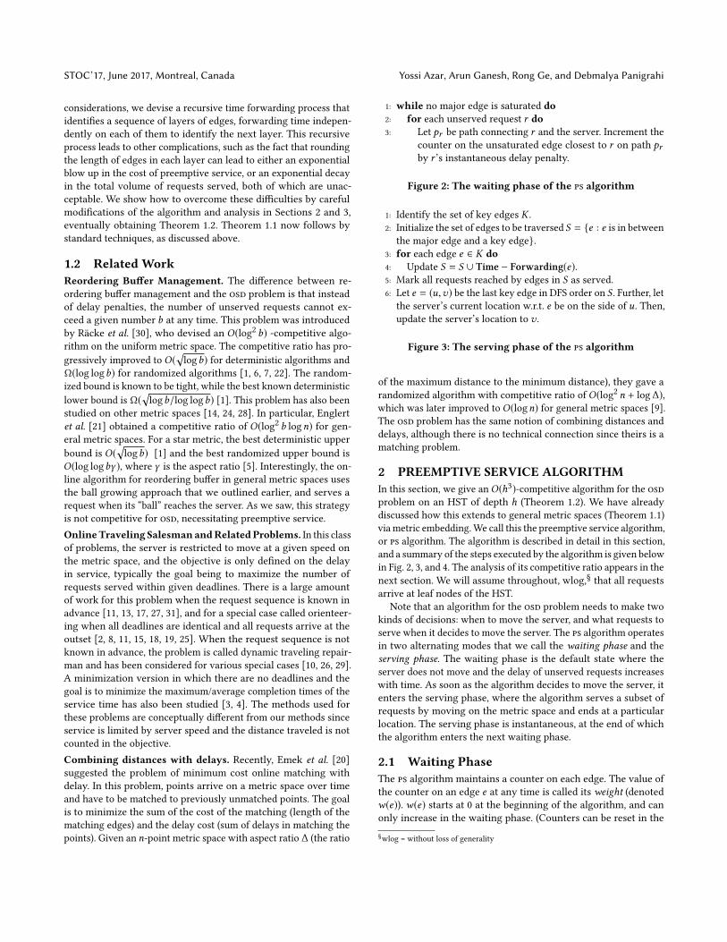
1: while no major edge is saturated do2: for each unserved request r do3: Let pr be path connecting r and the server. Increment the

counter on the unsaturated edge closest to r on path prby r ’s instantaneous delay penalty.

Figure 2: The waiting phase of the ps algorithm

1: Identify the set of key edges K .

2: Initialize the set of edges to be traversed S = e : e is in between

the major edge and a key edge.3: for each edge e ∈ K do4: Update S = S ∪ Time − Forwarding(e).5: Mark all requests reached by edges in S as served.

6: Let e = (u,v) be the last key edge in DFS order on S . Further, let

the server’s current location w.r.t. e be on the side of u. Then,

update the server’s location to v .

Figure 3: The serving phase of the ps algorithm

of the maximum distance to the minimum distance), they gave a

randomized algorithm with competitive ratio of O(log2 n + log∆),which was later improved to O(logn) for general metric spaces [9].

The osd problem has the same notion of combining distances and

delays, although there is no technical connection since theirs is a

matching problem.

2 PREEMPTIVE SERVICE ALGORITHMIn this section, we give an O(h3)-competitive algorithm for the osd

problem on an HST of depth h (Theorem 1.2). We have already

discussed how this extends to general metric spaces (Theorem 1.1)

via metric embedding. We call this the preemptive service algorithm,

or ps algorithm. The algorithm is described in detail in this section,

and a summary of the steps executed by the algorithm is given below

in Fig. 2, 3, and 4. The analysis of its competitive ratio appears in the

next section. We will assume throughout, wlog,§

that all requests

arrive at leaf nodes of the HST.

Note that an algorithm for the osd problem needs to make two

kinds of decisions: when to move the server, and what requests to

serve when it decides to move the server. The ps algorithm operates

in two alternating modes that we call the waiting phase and the

serving phase. The waiting phase is the default state where the

server does not move and the delay of unserved requests increases

with time. As soon as the algorithm decides to move the server, it

enters the serving phase, where the algorithm serves a subset of

requests by moving on the metric space and ends at a particular

location. The serving phase is instantaneous, at the end of which

the algorithm enters the next waiting phase.

2.1 Waiting PhaseThe ps algorithm maintains a counter on each edge. The value of

the counter on an edge e at any time is called its weight (denoted

w(e)). w(e) starts at 0 at the beginning of the algorithm, and can

only increase in the waiting phase. (Counters can be reset in the

§wlog = without loss of generality


1: Initialize the output set of edges S = ∅.2: Let time t be the rst (future) time when e is over-saturated by

the unserved requests in Xe .

3: for each unserved request r in Xe that is critical at time t do4: Let pr be the path connecting r to e .

5: Update S = S ∪ e ′ ∈ pr .6: if there exists some unserved request in Xe that is not critical

at time t then7: Let G(e) be the set of saturated edges that are not over-

saturated themselves, but their path to e contains only over-

saturated edges.

8: Select H (e) ⊆ G(e) such that

∑e ′∈H (e) `(e ′) = `(e).

9: for each edge e ′ ∈ H (e) do10: Update S = S ∪ Time − Forwarding(e ′).11: return S .

Figure 4: The subroutine Time-Forwarding(e) used in the psalgorithm

serving phase, i.e., we set to 0, which we describe later.) At any

time, the algorithm maintains the invariant that we ≤ `(e), where

l(e) is the length of edge e .

When a counter reaches its maximum value, i.e.,w(e) = `(e), we saythat edge e is saturated.

During the waiting phase, every unserved request increases the

counter on some edge on the path between the request and the

current location of the server. We will ensure that this is always

feasible, i.e., all edges on a path connecting the server to an un-

served request will not be saturated. In particular, every unserved

request increments its nearest unsaturated counter on this path by

its instantaneous delay penalty. Formally, let cr (τ ) denote the delay

penalty of a request r for a delay of τ . Then, in an innitesimal time

interval [t , t + ϵ], every unserved request r (say, released at time

tr ) contributes c′r (t − tr ) = cr (t − tr + ϵ) − cr (t − tr ) weight to the

nearest unsaturated edge on its path to the server.

Now, we need to decide when to end a waiting phase. One natural

rule would be to end the waiting phase when all edges on a request’s

path to the server are saturated. However, using this rule introduces

some technical diculties. Instead, note that in an HST, the length

of the entire path is at most O(1) times the maximum length of an

edge on the path. This allows us to use the maximum-length edge

as a proxy for the entire path.

For each request, we dene its major edge to be the longest edge onthe path from this request to the server. If there are two edges withthe same length, we pick the edge closer to the request.

A waiting phase ends as soon as any major edge becomes saturated.

If multiple major edges are saturated at the same time, we break

ties arbitrarily. Therefore, every serving phase is triggered by a

unique major edge.

2.2 Serving PhaseIn the serving phase, the algorithm needs to decide which requests

to serve. A natural choice is to restrict the server to requests whose

major edge triggered the serving phase. This is because it might

2i+1

2i-1 2i-1 2i-2

2i-3

2i-42i-32i-2

2i-22i-2

2i-2

2i 2i2i-1

2i-1 2i-2

2i-3

2i-42i-2

2i-22i-2

2i-22i-3

Figure 5: Example where major edge is not the parent of the rele-vant subtree. The major edge is in red, the key edges in yellow, andthe red circle is the location of the algorithm’s server. In this situ-ation, the server is in Te as shown and Xe = Re . The dotted boxesshow the edges in the critical subtree Ce . In particular, the gureon the right shows the transformation of the critical subtree, wherethemajor edge is now depicted as the parent of the relevant subtree.

be prohibitively expensive for the server to reach other requests in

this serving phase.

The relevant subtree of an edge e (denoted Re ) is the subtree ofvertices for which e is the major edge.We rst prove that the relevant subtree Re is a subtree of the HST,

where one of the ends of e is the root of Re .

Lemma 2.1. The major edge is always connected to the root of therelevant subtree.

Proof. Let r be the root of the relevant subtree (not including

the major edge). If the server is at a descendant of r , then by struc-

ture of the HST, the longest edge must be the rst edge from r to the

server (this is the case in Fig. 5). If the server is not at a descendant

of r , then the longest edge from the relevant subtree to the server

must be the edge connecting r and its parent. In either case, the

lemma holds.

There are two possible congurations of the major edge e vis-à-

vis its relevant subtree Re . Either e is the parent of the top layer of

edges in Re , or e is a sibling of this top layer of edges (see Fig. 6 for

examples of both situations). In either case, the denition of major

edge implies that the length of e is at least 2 times the length of anyedge in Re .

The ps algorithm only serves requests in the relevant subtree Reof the major edge e that triggered the serving phase. Recall from

the introduction that the algorithm performs two kinds of service:

critical service and preemptive service. First, we partition unserved

requests in Re into two groups.

Unserved requests in the relevant subtree Re that are connected to themajor edge e by saturated edges are said to be critical, while otherunserved requests in Re are said to be non-critical.The algorithm serves all critical requests in Re in the serving phase.

This is called critical service. In addition, it also serves a subset of

non-critical requests in Re as preemptive service. Next, we describe

the selection of non-critical requests for preemptive service.

Preemptive Service. We would like to piggyback the cost of pre-

emptive service on critical service. Let us call the subtree connecting

the major edge e to the critical requests in Re the critical subtree


2i+1

2i-1 2i-1 2i-2

2i-3 2i-42i-32i-2

2i-22i-2

2i-2

2i

2i

2i-1 2i-12i-2

2i-3 2i-42i-32i-2

2i-22i-22i-2

2i

Figure 6: The two possible congurations of themajor edge (in red)vis-à-vis the relevant subtree. The subtree surrounded by dashedbox is the relevant subtree. The red nodes are possible locations ofthe server. The edges in yellow are key edges. In the gure to theright, note that the edge of length 2

i to the right is not included inthe relevant subtree.

Ce (we also include e inCe ). Recall that e may either be a sibling or

the parent of the top layer of edges in Re (Fig. 6). Even in the rst

case, inCe , we make e the parent of the top layer of edges in Re for

technical reasons (see Fig. 5 for an example of this transformation).

Note that this does not violate the HST property of Ce since the

length of e is at least 2 times that of any other edge in Re , by virtue

of e being the major edge for all requests in Re .

The cost of critical service is the total length of edges in the criti-

cal subtreeCe . However, using this as the cost bound for preemptive

service in the ps algorithm causes some technical diculties. Rather,

we identify a subset of edges (we call these key edges) in Ce whose

total length is at least 1/h times that of all edges in Ce . We dene

key edges next.

Let us call two edges related if they form an ancestor-descendant

pair in Ce . A cut in Ce is a subset of edges, no two of which are

related, and whose removal disconnects all the leaves of Ce from

its root.

The set of key edges is formed by the cut of maximum total edgelength in the critical subtree Ce . If there are multiple such cuts, anyone of them is chosen arbitrarily.The reader is referred to Fig. 6 for an example of key edges. Note

that either the major edge e is the unique key edge, or the key edges

are a set of total length at least `(e) whose removal disconnects efrom all critical requests in the relevant subtree Re . It is not dicult

to see that the total length of the key edges is at least 1/h times

that of all edges in Ce .

We will perform recursive time forwarding on the key edges to

identify the requests for preemptive service. Consider any single

key edge e . Let us denote the subtree below e in the HST by Te .

Typically, when we are forwarding time on a key edge e , we consider

requests in subtree Te . However, there is one exception: if e is the

major edge and is a sibling of the top layer of its relevant subtree

(Fig. 6), then we must consider requests in the relevant subtree Re .

We dene a single notation for both cases:

For any key edge e , let Xe denote the following:• If the algorithm’s server is not in Te , then Xe = Te .• If the algorithm’s server is in Te , then Xe = Re .

To serve critical requests, the server must traverse a key edge eand enter Xe . Now, suppose Xe looks exactly like Fig. 1, i.e., there

is a single critical request and many non-critical requests. As we

saw in the introduction, the server cannot aord to only serve the

critical request, but must also do preemptive service. Our basic

principle in doing preemptive service is to simulate future time and

serve requests in Xe that would become critical the earliest. So, we

forward time into the future, which causes the critical subtree in

Xe to grow. But, our total budget for preemptive service in Xe is

only `(e), the length of e . (This is because the overall budget for

preemptive service in this serving phase is the sum of lengths of all

the key edges. This budget is distributed by giving a budget equal to

its length to each key edge.) This budget cap implies that we should

stop time forwarding once the critical subtree in Xe has total edge

length `(e); otherwise, we will not have enough budget to serve

the requests that have become critical after time forwarding. As

was the case earlier, working with the entire critical subtree in Xeis technically dicult. Instead, we forward time until there is a cut

in the critical subtree of Xe whose total edge length is equal to `(e)(at this point, we say edge e is over-saturated). This cut now forms

the next layer of edges in the recursion (we call these service edges).Note that the key edges form the rst layer of service edges in the

recursion. Extending notation, Xe ′ = Te ′ for all service edges in

subsequent layers of recursion. We recursively forward time on

each of these service edges e ′ in their respective subtrees Xe ′ using

the same process.

How does the recursion stop? Note that if the current service

edge e ′ is a leaf edge, then the recursion needs to stop since the only

vertex in Xe ′ is already critical at the time the previous recursive

level forwarded to. More generally, if all requests in Xe ′ become

critical without any cut in the critical subtree of Xe ′ attaining total

length `(e ′), then we are assured that the cost of serving all requests

in Xe ′ is at most h times the cost of traversing edge e ′. In this

case, we do not need to forward time further on e ′ (indeed, time

forwarding does not change the critical subtree since all requests

are already critical), and the recursion ends.

We now give a formal description of this recursive time forward-

ing process. For any edge e , let child(e) be the edges in the rst

layer of subtree Xe . (When Xe = Te , these are simply the children

edges of e . But, in the special case where Xe = Re , these are the

siblings of e of smaller length than e .) We dene

f (e) =max

(`(e),∑ei ∈child(e) f (ei )

)if e is saturated.

0 otherwise.

This allows us to formally dene over-saturation, that we intuitively

described above.

An edge e is said to be over-saturated if either of the followinghappens:

• e is saturated and∑ei ∈child(e) f (ei ) ≥ `(e), i.e., f (e) is

determined by∑ei ∈child(e) f (ei ) in the formula above (we

call this over-saturation by children).• All requests in Xe are connected to e via saturated edges.

Using this notion of over-saturation, the ps algorithm now identies

a set of edges S that the server will traverse in the relevant subtree

Re of the major edge e that triggered the serving phase. In the

formal description, we will not consider critical service separately

since the edges in the critical subtree Ce will be the rst ones to be


added to S in our recursive Time-Forwarding process. Initially,

all saturated edges between the key edges and the major edge, both

inclusive, are added to S . This ensures that the algorithm traverses

each key edge. Now, the algorithm performs the following recursive

process on every key edge e ′ in subtree Xe .

Intuitively, the edges inG(e) are the ones that form the maximum

length cut in the critical subtree of Xe at time t (we show this

property formally in Lemma 3.3). In the recursive step, ideally we

would like to recurse on all edges in G(e). However, if el is the last

edge added toG(e) during Time-Forwarding(e), it is possible that∑e ′∈G(e)\el `(e

′) < f (e) but

∑e ′∈G(e) `(e ′) > f (e). In this case,

we cannot aord to recurse on all edges in G(e) since their total

length is greater than that of e . This is why we select the subset

H (e) whose sum of edge lengths is exactly equal to that of e . We

show in Lemma 2.2 below that this is always possible to do. The

set of edges that we call Time-Forwarding on, i.e., the key edges

and the union of all H (e)’s in the recursive algorithm, are called

service edges.

Lemma 2.2. Let e be an edge oversaturated by children.G(e) rep-resents a set of saturated but not over-saturated edges satisfying:∑

e ′∈G(e)`(e ′) =

∑e ′∈G(e)

f (e ′) ≥ `(e).

Then, there is some subset H (e) ⊆ G(e) such that∑e ′∈H (e) `(e ′) =

`(e).

Proof. Note that all edge lengths are of the form 2i

for non-

negative integers i . Furthermore, the length of every edge inG(e) isstrictly smaller than the length of e . Thus, the lemma is equivalent

to showing that for any set of elements of the form 2i

(for some

i ≤ j − 1) that sum to at least 2j, there exists a subset of these

elements that sum to exactly 2j.

First, note that we can assume that the sum of these elements

is strictly smaller than (3/2) · 2j . If not, we repeatedly discard an

arbitrarily selected element from the set until this condition is met.

Since the discarded value is at most 2j−1

at each stage, the sum

cannot decrease from ≥ (3/2) · 2j to < 2j

in one step.

Now, we use induction on the value of j. For j = 1, the set can

only contain elements of value 20 = 1, and sums to the range [1, 3).

Clearly, the only option is that there are two elements, both of value

1. For the inductive step, order the elements in decreasing value.

There are three cases:

• If there are 2 elements of value 2j−1

, we output these 2

elements.

• If there is 1 element of value 2j−1

, we add it to our output

set. Then, we start discarding elements in arbitrary order

until the remaining set has total value less than (3/2) · 2j−1.

Then, we apply the inductive hypothesis on the remaining

elements.

• Finally, suppose there is no element of value 2j−1

in the

set. We greedily create a subset by adding elements to the

subset in arbitrary order until their sum is at least 2j−1

.

Since each element is of value at most 2j−2

, the total value

of this subset is less than (3/2) · 2j−1. Call this set A. Now,

we are left with elements summing to total value at least

2j−1

and less than 2j. We again repeat this process to obtain

another set B of total value in the range [2j−1, (3/2) · 2j−1).We now recurse on these two subsets A and B.

Once all chains of recursion have ended, the server does a DFS

on the edges in S , serving all requests it encounters in doing so.

After this, the server stops at the bottom of the last key edge visited.

Remark: If the HST is an embedding of a general metric space, then

the leaves in the HST are the only actual locations on the metric

space. So, when the ps algorithm places the server at an intermediate

vertex, the server is actually sent to a leaf in the subtree under that

vertex in the actual metric space. It is easy to see that this only

causes a constant overhead in the service cost. Note that this does

not aect the ps algorithm’s operation at all; it operates as if the

server were at the non-leaf vertex.

Finally, the algorithm resets the counters, i.e., sets w(e) = 0, for

all edges e that it traverses in the serving phase.

This completes the description of the algorithm.

3 COMPETITIVE RATIO OF PREEMPTIVESERVICE ALGORITHM

In this section, we show that the ps algorithm described in the

previous section has a competitive ratio ofO(h3) on an HST of depth

h (Theorem 1.2), which implies a competitive ratio of O(log4 n) on

general metric spaces (Theorem 1.1).

First, we specify the location of requests that can put weight on

an edge at any time in the ps algorithm.

Lemma 3.1. At any time, for any edge e , the weight on edge e isonly due to unserved requests in Xe .

Proof. When the server serves a request, it traverses all edges

on its path to the request and resets their respective counters. So,

the only possibility of violating the lemma is due to a change in

the denition of Xe . But, for the denition of Xe to change, the

server must traverse edge e and reset its counter. This completes

the proof.

Next, we observe that the total delay penalty of the algorithm

is bounded by its service cost. (Recall that the service cost is the

distance moved by the server.)

Lemma 3.2. The total delay penalty is bounded by the total servicecost.

Proof. By design of the algorithm, every unserved request al-

ways increases the counter on some edge with its instantaneous

delay penalty. The lemma now follows from the observation that

the counter on an edge e can be reset from at most `(e) to 0 only

when the server moves on the edge incurring service cost `(e).

Next, we show that the total service cost can be bounded against

the length of the key edges. First, we formally establish some prop-

erties of the Time-Forwarding process that we intuitively stated

earlier.

Lemma 3.3. When the algorithm performsTime-Forwarding(e), then the following hold:

• If a saturated edge e ′ ∈ Xe is not over-saturated by itschildren, all cuts in the saturated subtree in Xe ′ have totaledge length at most `(e ′).


• ∑e ′∈G(e) `(e ′) ≤ (3/2)`(e).

• G(e) is the cut of maximum total edge length in the saturatedsubtree ofXe at time t , the time when e is rst over-saturated.

Proof. The rst property follows from the fact that for a satu-

rated edge e ′, the denition of the function f (.) implies that the

value of f (e ′) is at least the sum of lengths of any cut in the satu-

rated subtree of Xe ′ at time t .For the second property, note that every edge in Xe has length

at most `(e)/2, and use Lemma 2.2.

Now, suppose the third property is violated, and there is a larger

saturated cut G ′(e). Since G(e) over-saturates all its ancestor edges,

it follows that for any such ancestor edge e in Xe , the descendants

of e in G(e) have total length at least `(e). Thus, there must be an

edge e∗ ∈ G(e) such that the sum of lengths of the descendants of

e∗ in G ′(e) is greater than `(e∗). But, if this were the case, e∗ would

be over-saturated, which contradicts the denition of G(e).

Lemma 3.4. The total service cost is at most O(h2) times the sumof lengths of key edges.

Proof. By the HST property, the distance traveled by the server

from its initial location to the major edge e is at mostO(1) times `(e).But, `(e) is at most the total length of the key edges, since e itself

is a valid cut in the critical subtree Ce . Hence, we only consider

server movement in the relevant subtree Re .

Now, consider the edges connecting the major edge to the key

edges. Let the key edges have total length L. Consider the cut com-

prising the parents of all the key edges. They also form a valid cut,

and hence, their total length is at most L. We repeat this argument

until we get to the major edge. Then, we have at most h cuts, each

of total edge length at most L. Thus the total length of all edges

connecting the major edge to the key edges is at most h times the

length of the key edges.

This brings us to the edges traversed by the server in the subtrees

Xe , for key edges e . We want to bound their total length by O(h2 ·`(e)). We will show a more general property: that for any serviceedge e , the total length of edges traversed in Xe is O(h2 · `(e)).First, we consider the case that the recursion ends at e , i.e., e was

not over-saturated by its children. By Lemma 3.3, this implies that

every cut in the saturated subtree in Xe has total length at most

`(e). In particular, we can apply this to the layered cuts (children of

the key edges, their children, and so on) in the saturated subtree.

There are at most h such cuts covering the entire saturated subtree,

implying that the total cost of traversing the saturated edges in Xeis O(h · `(e)).

Next, we consider the case when e is over-saturated by its chil-

dren. We use an inductive argument on the height of the subtree

Xe . Suppose this height is h. Further, let the edges in H (e) (that

we recurse on in Time-Forwarding(e)) be e1, e2, . . ., where the

height of subtree Xei is hi ≤ h − 1. By denition of H (e), we have∑i `(ei ) = `(e). Using the inductive hypothesis, the total cost inside

subtree Xei is at most C · h2i · `(ei ) for some constant C . Summing

over i , and using hi ≤ h − 1, we get that the total cost is at most

C · (h− 1)2 · `(e). This leaves us with the cost of reaching the critical

requests in X (e ′) for each e ′ ∈ G(e), from edge e . We can partition

these edges into at most h layers, where by Lemma 3.3, the total

cost of each such layer is at most (3/2) · `(e). It follows that the

total cost of all layers is at most (3/2) · h · `(e). Adding this to the

inductive cost, the total cost is at mostC ·h2 ·`(e) for a large enough

C . This completes the inductive proof.

Now, we charge the lengths of all key edges to the optimal

solution opt. Most of the key edges will be charged directly to

opt, but we need to dene a potential function Φ for one special

case. For a xed optimal solution, we dene Φ as

Φ = κd(alg’s server, opt’s server).In words, Φ is equal to κ times the distance between algorithm’s

server and opt’s server. Here, κ = ch2 for a large enough constant

c . Overall, we use a charging argument to bound all costs and

potential changes in our algorithm to opt such that the charging

ratio is O(h3).The rst case is when the major edge e is the only key edge, and

opt’s server is in Xe . Then, all costs are balanced by the decrease

in potential.

Lemma 3.5. When the major edge e is the only key edge, and opt’sserver is in Xe , the sum of change in potential function Φ and theservice cost is non-positive.

Proof. This is immediate from the denition ofΦ and Lemma 3.4.

In other cases, we charge all costs and potential changes to either

opt’s waiting cost or opt’s moving cost by using what we call a

charging tree.A charging tree is a tree of (service edge, time interval) pairs. Foreach service edge e at time t , let t ′ be the last time that e was a serviceedge (t ′ = 0 if e was never a service edge in the past). Then, (e, [t ′, t))is a node in a charging tree. We simultaneously dene a set of chargingtrees, the roots of which exactly correspond to nodes (e, [t ′, t)) wheree is a key edge at time t .

To dene the charging trees, we will specify the children of a node(e, [t ′, t)):

• The node (e, [t ′, t)) is a leaf in the charging tree if t ′ = 0 or eis not over-saturated by children at time t ′ (i.e., all previouslyunserved requests in Xe were served at time t ′).

• Otherwise, let H (e) be as dened in Time-Forwarding(e).For any e ′ ∈ H (e), let t ′′ be the last time that e ′ was aservice edge. Then, for each e ′ ∈ H (e), (e ′, [t ′′, t ′)) is a childof (e, [t ′, t)).

See Fig. 7 for an example. This gure shows a charging tree with 5

nodes: (e, [t2, t1)), (e1, [t4, t2)), (e2, [t3, t2)), (e11, [t5, t4)), (e12, [t6, t4)).We say that opt incurs moving cost at a charging tree node

(e, [t ′, t)) if it traverses edge e in the time interval [t ′, t). Next, we

incorporate opt’s delay penalties in the charging tree. We say that

opt incurs waiting cost of `(e) at a charging tree node (e, [t ′, t)), if

there exists some (future) time t∗ ≥ t such that:

• opt’s server is never in Xe in the time interval [t ′, t∗), and

• the requests that arrive in Xe in the time interval [t ′, t)have a total delay penalty of at least `(e) if they remain

unserved at time t∗.

Intuitively, if these conditions are met, then opt has a delay penalty

of at least `(e) from only the requests in subtree Te that arrived in

the time interval [t ′, t).


e

e1

e2

e11

e12time

t1t2t5 t4 t3t6 edges

(e, [t2,t1))

(e1, [t4,t2)) (e2, [t3,t2))

(e11, [t5,t4)) (e12, [t6,t5))

charging tree

Figure 7: Example of a charging tree. On the top is the timelinecorresponding to the charging tree on the bottom. The blue circlesrepresent that the corresponding edge is a service edge in the serv-ing phase of the algorithm at that time. The red circle indicates thatopt’s server traverses the edge in the interval dened the two bluecircles surrounding the red circle. The green circle indicates that thecorresponding edge is not only a service edge in the serving phaseof the algorithm at that time, but that the algorithm actually servedall requests in the corresponding subtree Xe12 .

Without loss of generality, we assume that at time 0, opt tra-

verses all the edges along the paths between the starting location of

the server and all requests. (Since these edges need to be traversed

at least once by any solution, this only incurs an additive cost in

opt, and does not change the competitive ratio by more than a

constant factor.)

Now, we prove the main property of charging trees.

Lemma 3.6 (Main Lemma). For any key edge e served at time tby the algorithm, if opt’s server was not in Xe at time t , then opt’swaiting and moving cost in the charging tree rooted at (e, [t ′, t)) is atleast `(e).

Proof. We use the recursive structure of the charging tree. Sup-

pose the root of the tree is (e, [t ′, t)), the current node we are consid-

ering is (u, [t ′u , tu )), and the parent of the current node is (v, [t ′v , tv )).(Here, u and v are edges in the HST.) By the structure of the charg-

ing tree, we know that t ′v = tu . We will now list a set of conditions.

At node (u, [t ′u , tu )), if one of these conditions holds, then we show

that the waiting or moving cost incurred by opt at this node is

at least `(u), the length of edge u. Otherwise, we recurse on all

children of this charging tree node. The recursion will end with

one these conditions being met.

Case 1. opt crossed edge u in the time interval [t ′u , tu ): This is the

case for (e2, [t3, t2)) in Fig. 7. In this case, opt incurs moving cost

of `(u) at node (u, [t ′u , tu )) of the charging tree.

Case 2. Case 1 does not apply, and the algorithm forwarded time togreater than t in Time-Forwarding(u) at time t ′u : This is the case

for (e11, [t5, t4)) in Fig. 7. A detailed illustration of this case is given

in Fig. 8. Note that Case 1 does not apply to (u, [t ′u , tu )) by denition.

Moreover, Case 1 also does not apply to any of the ancestors of this

node in the charging tree; otherwise, the recursive charging scheme

would not have considered the (u, [t ′u , tu )) node. Furthermore, at

e1

e11

e1

e11

Time forwarding from t5 to > t1 on e11

Time forwarding from t4 to < t1 on e1

e1

e11

Requests below e11

at time t4

Figure 8: Illustration of Case 2 in Lemma 3.6. The left gure showsthe time forwarding for e11 at time t5. All the red requests are servedat t5. The center gure shows the waiting time below e11 at time t4.Note that since t4 < t , the yellow requests could not reach e11, andthe green requests are requests that came between t5 and t4. Theright gure shows the time forwarding process for e1 at time t4. Weknow e11 must be saturated because it is a child in charging tree.However, the yellow requests cannot contribute to e11 because theydo not even reach e11 at time t . Therefore, all the weight on e11 mustcome from green requests.

time t , opt’s server was not in Xe by the condition of the lemma.

These facts, put together, imply that opt could not have served

any request in Xu in the time interval [t ′u , t) . In particular, this

implies that opt could not have served requests in Xu that arrived

in the time interval [t ′u , tu ) before time t (these are green requests

in Fig. 8).

We now need to show that these requests have a total delay

penalty of at least `(u) by time t . Since Time-Forwarding(u) for-

warded time beyond t at time t ′u , any request in Xu that arrived

before t ′u and put weight on edge u (these are red requests in Fig. 8)

must have been served at time t ′u . The requests left unserved (yel-

low requests in Fig. 8) do not put weight on edge u even after

forwarding time to t .Now, note that no ancestor of the (u, [t ′u , tu )) node in the charg-

ing tree can be in Case 2, else the recursive charging scheme would

not consider the (u, [t ′u , tu )) node. Therefore,Time-Forwarding(v)

must have forwarded time to at most t at time t ′v = tu . Suppose we

reorder requests so that the requests that arrived earlier put weight

rst (closer to the request location), followed by requests that ar-

rived later. Then, the requests in Xu that arrived before t ′u but were

not served at time t ′u (yellow requests in Fig. 8) do not put weight

on edge u in Time-Forwarding(v) at time t ′v , since time is being

forwarded to less than t . Therefore, the only requests in Xu that

put weight on edge u in Time-Forwarding(v) at time t ′v arrived

in the time interval [t ′u , tu ) (green requests in Fig. 8). By Lemma 3.1,

at any time, the only requests responsible for the weight on edge

u are requests in Xu . Therefore, the requests that arrived in Xu in

the time interval [t ′u , tu ) saturate edge e in Time-Forwarding(v)

at time t ′v . In other words, these requests incur delay penalties of

at least `(u) if they are not served till time t . Since opt did not

serve any of these requests before time t , it follows that opt incurs

waiting cost of `(u) at node (u, [t)u ′, tu )) of the charging tree.

Case 3. Case 1 does not apply, and all requests in Xu were served bythe algorithm at time t ′u : This is the case for (e12, [t6, t4)) in Fig. 7.

Similar to the previous case, Time-Forwarding(v) at time t ′v must


have been to at most time t . Since all requests in Xu that arrived

before time t ′u were served at time t ′u , the requests that saturated

edge u in Time-Forwarding(v) at time t ′v = tu must have arrived

in the time interval [t ′u , tu ) (same argument as in Case 2). As in

Case 2, opt could not have served these requests before time t ,and hence incurs delay penalty of at least `(u) on these requests.

Therefore, opt incurs waiting cost of `(u) at node (u, [t ′u , tu )) of the

charging tree.

By the construction of charging tree, the leaves are either in

Case 3, or has starting time 0 (which is in Case 1). So, this recursive

argument always terminates.

Note that each key edge is the root of a charging tree, and for

each node of the charging tree, the length of the corresponding

edge is equal to the sum of lengths of the edges corresponding to its

children nodes. Therefore when the argument terminates, we can

charge the cost of the key edge to a set of nodes in the charging tree

whose total cost is exactly equal to the cost of the key edge.

So, we have shown that the length of key edges can be bounded

against opt’s cost on the charging tree. But, it is possible that in this

analysis, we are using the same cost incurred by opt in multiple

charging tree nodes. In other words, we need to bound the cost

incurred by opt at charging tree nodes against the actual cost of

opt.

Lemma 3.7. The total number of charging tree nodes on which thesame request causes opt to incur cost is at most h + 1.

Proof. First, note that the charging tree nodes corresponding

to the same edge e represent disjoint time intervals. This implies

that for a given request that arrived at time t , opt only incurs cost

in the charging tree node (e, [t1, t2)) where t ∈ [t1, t2). We now

show that the total number of dierent edges for which the same

request is counted toward opt’s cost at charging tree nodes is at

most h + 1.

To obtain this bound, we observe that there are two kinds of

edges we need to count: (1) edges on the path from the request to

the root of the HST, and (2) edges for which the request is in the

relevant subtree. Clearly, there are at most h category (1) edges. But,

there can be a much larger number of category (2) edges. However,

we claim that among these category (2) edges, opt incurs cost in

the charging tree at a node corresponding to at most one edge. To

see this, we observe the following properties:

• If opt incurs cost at a charging tree node corresponding

to a category (2) edge e , then opt’s server must be in Te at

the arrival time of the request.

• The category (2) edges are unrelated in the HST, i.e., for

any two such edges e1, e2, we have the property that Te1and Te2 are disjoint.

Finally, we are ready to prove the main theorem (Theorem 1.2).

Proof of Theorem 1.2. Recall that we bound both the delay

penalties and service cost of the algorithm by the total length of

key edges times O(h2), in Lemmas 3.2 and 3.4. Now, we will charge

the total length of key edges to O(h) times opt’s costs. Consider a

serving phase at time t .

Case (a). Suppose opt’s server is not in subtree Xe of a key edge

e . Then, by Lemma 3.6, opt incurs a cost of at least `(e) in the

charging tree rooted at (e, [t ′, t)), where t ′ is the last time when ewas a service edge. On the other hand, opt’s moving cost can be

counted by at most one node in all charging trees, and by Lemma 3.7,

opt’s waiting cost can be counted by at most h + 1 nodes in all

charging trees. Therefore the total length of Case (a) key edges is

bounded by (h + 1) times the cost of opt.

Case (b). Now, let us consider the situation where opt’s server is

in the subtree Xe for a key edge e . There are two possibilities:

• Case (b)(i). If e is also the major edge, it must be the unique

key edge and we apply Lemma 3.5.

• Case (b)(ii). Otherwise, e is not the major edge. Then, any

single key edge can be of length at most half the major

edge, but the key edges add up to at least the length of the

major edge. Thus, any single key edge only accounts for at

most half the total length of key edges. Now, opt’s server

can be in the subtree Te for only one of the key edges e(note that in this case, Te = Xe since the major edge is

not the unique key edge). It follows that the key edges in

Case (a) account for at least half the total length of the key

edges. In this case, we can charge the Case (b) key edges

to the Case (a) key edges (which are, in turn, charged to

opt by the argument above).

Finally, we also need to bound the change in potential during

this serving phase in Case (a) and Case (b)(ii). Note that if e is the

major edge, the server’s nal location is at a distance of at most

4`(e) from the server’s initial solution (the server rst reaches the

major edge, then crosses the major edge, and eventually ends on

the other side of some key edge). Therefore, the total change in

potential is at most 4κ`(e), which is also bounded by O(h2) times

the total length of the key edges.

4 SPECIAL METRICSIn this section, we present algorithms for the k-osd problem on

special metric spaces: uniform and star metrics. These respectively

correspond to the paging and weighted paging problems with delay.

4.1 Uniform Metric/PagingWe give a reduction from the k-osd problem on a uniform metric to

the classical online paging problem. The reduction is online, non-

clairvoyant, and preserves the competitive ratio up to a constant.

To describe this reduction, it would be convenient to view the k-osd

problem on a uniform metric as the following equivalent problem

that we call paging with delay:

There are n pages that issue requests over time. Each request is servedwhen the corresponding page is brought into a cache that can onlyhold k < n pages at a time. The algorithm can bring a page intothe cache and evict an existing page, this process being called a page

swap and having a cost of one. For every request, the algorithm alsoincurs a delay penalty, which is a monotone function of the delay inserving the request. The algorithm can only access the current valueof the delay penalty.

Classical paging is the special case of this problem when every

request has an innite delay penalty, i.e., each request must be

served immediately, and the total cost is the number of page swaps.


Paging with delay time

Classical Paging time

(a) The reduction between instances for un-weighted paging. This gure shows the re-quests for a single page.Paging with delay time

Classical Paging time

Request for page of weight 1

Request for page of weight W

Delay penalty =Weight of waiting request

(b) An example where the reduction has alarge gap for weighted paging.

Figure 9: The reduction between instances of online paging withdelay and classical online paging: it works for unweighted paging,but fails for weighted paging.

Suppose we are given an instance I of the paging problem with

delay. We will reduce it to an instance I ′ of classical online paging.

The requests for a page p in I are partitioned into time intervals

such that the total delay penalty incurred by the requests in an

interval is exactly one at the end of the interval. In instance I ′, this

interval is now replaced by a single request for p at the end of the

interval. (See Fig. 9a.) Note that the reduction is online and non-

clairvoyant. We now show that by this reduction, any algorithm

for I ′ can be used for I, losing only a constant in the competitive

ratio.

Lemma 4.1. The optimal cost in I ′ is at most 3 times the optimalcost in I. Conversely, the cost of an algorithm in I is at most 2 timesthat in I ′.

Proof. Let us denote the optimal costs in I and I ′ by optIand optI′ respectively. Similarly, let algI and algI′ respectively

denote the cost an algorithm in I and I ′.Construct a solution for I ′ that maintains exactly the same

cache contents as the optimal solution for I at all times. Whenever

there is a request for a page that is not in the cache, it serves the

page and then immediately restores the cache contents of optI by

performing the reverse swap and restoring the previous page in the

cache. Note that there are two types of page swaps being performed:

the rst category are those that are also performed by optI , and

the second category are the pairs of swaps to serve requests for

pages not in the cache. The total number of page swaps in the rst

category is identical the number of page swaps in optI . For the

second category, if a page p is not in the cache at the end of an

interval in I, there are two possibilities. If no request for p in the

preceding interval was served in optI during the interval, then the

total delay penalty for these requests at the end of the interval is 1.

On the other hand, if some request for p in the preceding interval

was served in optI during the interval, but the page is no longer in

the cache at the end of the interval, then there was at least 1 page

swap that removed p from the cache during the interval. In either

case, we can charge the two swaps performed in I ′ to the cost of 1

that optI incurs in this interval for page p.

In the converse direction, note that by denition, the swap cost

of algI is identical to that of algI′ . The only dierence is that in

I, the algorithm also suers a delay penalty. The delay penalty for

a page in an interval is 0 if the algorithm maintains the page in the

cache throughout the interval, and at most 1 otherwise. In the latter

case, the algorithm must have swapped the page out during the

interval since the page was in the cache at the end of the previous

interval. In this case, we can charge the delay penalty in algI to

this page swap during the interval that algI′ incurred.

Using the above lemma and the well-known and asymptotically

tight O(k)-competitive deterministic and O(logk)-competitive ran-

domized algorithms for online paging (see, e.g., [16]), we obtain the

following theorem.

Theorem 4.2. There areO(k)-competitive deterministic andO(logk)-competitive randomized algorithms for online paging with delay(equivalently, k-osd on the uniform metric). This implies, in particu-lar, that there is an O(1)-competitive deterministic algorithm for osdon uniform metrics. These results also apply to the non-clairvoyantversion of the problems, where the delay penalties in the future are un-known to the algorithm. These competitive ratios are asymptoticallytight.

4.2 Star Metric/Weighted PagingAs in the case of the uniform metric, it will be convenient to view

the k-osd problem on a star metric as a paging problem with delay,

the only dierence being that every page p now has a non-negative

weight wp which is the cost of evicting the page from the cache.

Note that in this case the aspect ratio ∆ of the star metric is (up to

a constant factor) the ratio of the maximum and minimum page

weights.

For weighted paging, suppose we try to use the reduction strat-

egy for (unweighted) paging from the previous section. We can now

partition requests for a page p into intervals, where the total delay

penalty at the end of the interval is the weight of the page wp . This

reduction, however, fails even for simple instances. Consider two

pages of weightsW and 1, whereW 1. Suppose their requests

have penalty equal to their respective weights for unit delay. If the

requests for the pages alternate, and the cache can only hold only

a single page, the algorithm repeatedly swaps the pages, whereas

an optimal solution keeps the heavy page in the cache and serves

the light page only once everyW time units. The gap induced by

the reduction in this instance isW . (See Fig. 9b.)

Indeed, we show that this diculty is fundamental in that there

is no good non-clairvoyant algorithm for the weighted paging

problem with delay.

Theorem 4.3. There is a lower bound of Ω(W ) on the competitiveratio of weighted paging with delay, even with a single-page cache(equivalently, osd on a star metric) in the non-clairvoyant setting,


where W is the ratio of the maximum to minimum page weight(equivalently, aspect ratio ∆ of the star metric).

Proof. Suppose there is a heavy page p0 with cost W (with-

out loss of generality assumeW is an integer), and all other pages

p1,p2, ...,pn have cost 1. Set n =W 2. We will construct an adver-

sarial instance based on how the algorithm decides to serve the

pages. The instance is constructed in phases: at the beginning of

each phase, there is a request for all of the small pages p1, ...,pn .

However, the waiting cost for all of these requests start at 0, and

at some time t (not necessarily in the same phase) will become

innity; we say that this request becomes critical at time t . The

adversary will control the time that requests become critical. For

each phase, we maintain the following properties:

(1) At the beginning of each phase, all the small pages have a

request.

(2) The algorithm either serves all the small pages at least

once, or serves page p0 at leastW times, in each phase.

(3) The optimal solution does not incur any waiting cost. In

each phase, the optimal solution serves p0 once and at most

W of the small pages.

Given these properties, it is easy to check that the competitive ratio

of the algorithm is at leastW /2, because in each phase algorithm

spends at leastW 2, while the optimal spends at most 2W .

Now we describe how the adversary works. At time ϵ (for any

xed ϵ strictly between 0 and 1), there is a request for p0 that

requires immediate service. At time t = 1, 2, ...,W , if the algorithm

has not served all the small pages at least once in this phase, let rt ∈1, 2, ...,n denote the index of an unserved page. The adversary

makes prt critical at time t , and adds a request for p0 at time t + ϵ .

Note that page p0 must be in the algorithm’s cache at time t − 1+ ϵand at time t + ϵ , but cannot be in the algorithm’s cache at time

t . Thus, the algorithm must evict p0 at least once in this interval.

Therefore, at the end of timeW + 1, either the algorithm has served

all the small pages at least once in this phase, or it has served p0 at

leastW times.

The optimal solution serves pr1 , pr2 , . . . , prt at time 0, and p0at time ϵ . Since no other page became critical in this phase, the

optimal solution will never need to evict p0 in this phase.

After timeW + 1, the adversary generates a request for each of

the small pages, and starts a new phase. If this procedure repeats

for k phases, then the algorithm’s cost is at least kW 2, while the

optimal solution’s cost is at most 2kW + n (the optimal solution

serves all non-critical requests at the very end). Therefore, as kgoes to innity, the competitive ratio of the algorithm cannot be

better thanW /2.

The above theorem implies that we must restrict ourselves to

the clairvoyant setting for the weighted paging with delay problem.

For this case, our results for osd/k-osd on a star metric follow as

corollaries of our theorems for general metrics (Theorems 1.2, 1.3).

Theorem 4.4. There is an O(k)-competitive deterministic algo-rithm for online weighted paging with delay (equivalently, k-osd on astar metric). This implies, in particular, anO(1)-competitive determin-istic algorithm for the osd problem on star metrics. These competitiveratios are asymptotically tight for deterministic algorithms.

ACKNOWLEDGEMENTY. Azar was supported in part by the Israel Science Foundation

(grant No. 1506/16), by the I-CORE program (Center No.4/11) and

by the Blavatnik Fund. A. Ganesh and D. Panigrahi were supported

in part by NSF Awards CCF 1535972 and CCF 1527084. This work

was done in part while Y. Azar and D. Panigrahi were visiting the

Simons Insitute for Theoretical Computer Science, as part of the

Algorithms and Uncertainty program.

REFERENCES[1] Anna Adamaszek, Artur Czumaj, Matthias Englert, and Harald Räcke. 2011.

Almost tight bounds for reordering buer management. In STOC. 607–616.

[2] Esther M Arkin, Joseph SB Mitchell, and Giri Narasimhan. 1998. Resource-

constrained geometric network optimization. In SOCG. ACM, 307–316.

[3] Giorgio Ausiello, Esteban Feuerstein, Stefano Leonardi, Leen Stougie, and Maur-

izio Talamo. 1995. Competitive Algorithms for the On-line Traveling Salesman. In

Algorithms and Data Structures, 4th International Workshop, WADS ’95, Kingston,Ontario, Canada, August 16-18, 1995, Proceedings. 206–217.

[4] Giorgio Ausiello, Esteban Feuerstein, Stefano Leonardi, Leen Stougie, and Maur-

izio Talamo. 2001. Algorithms for the On-Line Travelling Salesman. Algorithmica29, 4 (2001), 560–581.

[5] Noa Avigdor-Elgrabli, Sungjin Im, Benjamin Moseley, and Yuval Rabani. 2015. On

the Randomized Competitive Ratio of Reordering Buer Management with Non-

Uniform Costs. In Automata, Languages, and Programming - 42nd InternationalColloquium, ICALP 2015, Kyoto, Japan, July 6-10, 2015, Proceedings, Part I. 78–90.

[6] Noa Avigdor-Elgrabli and Yuval Rabani. 2010. An Improved Competitive Algo-

rithm for Reordering Buer Management. In SODA. 13–21.

[7] Noa Avigdor-Elgrabli and Yuval Rabani. 2013. An Optimal Randomized Online

Algorithm for Reordering Buer Management. CoRR abs/1303.3386 (2013).

[8] Baruch Awerbuch, Yossi Azar, Avrim Blum, and Santosh Vempala. 1998. New

approximation guarantees for minimum-weight k-trees and prize-collecting

salesmen. SIAM J. Comput. 28, 1 (1998), 254–262.

[9] Yossi Azar, Ashish Chiplunkar, and Haim Kaplan. 2017. Polylogarithmic Bounds

on the Competitiveness of Min-cost Perfect Matching with Delays. In Proceedingsof the Twenty-eighth Annual ACM-SIAM Symposium on Discrete Algorithms, SODA2017, Barecelona, Spain.

[10] Yossi Azar and Adi Vardi. 2015. TSP with Time Windows and Service Time.

CoRR abs/1501.06158 (2015).

[11] Nikhil Bansal, Avrim Blum, Shuchi Chawla, and Adam Meyerson. 2004. Approx-

imation algorithms for deadline-TSP and vehicle routing with time-windows. In

STOC. ACM, 166–174.

[12] Nikhil Bansal, Niv Buchbinder, Aleksander Madry, and Joseph Naor. 2015. A

Polylogarithmic-Competitive Algorithm for the k-Server Problem. J. ACM 62, 5

(2015), 40.

[13] Reuven Bar-Yehuda, Guy Even, and Shimon Moni Shahar. 2005. On approximat-

ing a geometric prize-collecting traveling salesman problem with time windows.

Journal of Algorithms 55, 1 (2005), 76–92.

[14] Siddharth Barman, Shuchi Chawla, and Seeun Umboh. 2012. A Bicriteria Ap-

proximation for the Reordering Buer Problem. In ESA. 157–168.

[15] Avrim Blum, Shuchi Chawla, David R Karger, Terran Lane, Adam Meyerson, and

Maria Minko. 2003. Approximation algorithms for orienteering and discounted-

reward tsp. In Foundations of Computer Science, 2003. Proceedings. 44th AnnualIEEE Symposium on. IEEE, 46–55.

[16] Allan Borodin and Ran El-Yaniv. 1998. Online Computation and CompetitiveAnalysis. Cambridge University Press, New York, NY, USA.

[17] Chandra Chekuri and Nitish Korula. 2007. Approximation algorithms for orien-

teering with time windows. arXiv preprint arXiv:0711.4825 (2007).

[18] Chandra Chekuri, Nitish Korula, and Martin Pál. 2012. Improved algorithms for

orienteering and related problems. ACM Transactions on Algorithms (TALG) 8, 3

(2012), 23.

[19] Chandra Chekuri and Amit Kumar. 2004. Maximum coverage problem with

group budget constraints and applications. In Approximation, Randomization,and Combinatorial Optimization. Algorithms and Techniques. Springer, 72–83.

[20] Yuval Emek, Shay Kutten, and Roger Wattenhofer. 2016. Online matching: haste

makes waste!. In Proceedings of the 48th Annual ACM SIGACT Symposium onTheory of Computing, STOC 2016, Cambridge, MA, USA. 333–344.

[21] Matthias Englert, Harald Räcke, and Matthias Westermann. 2010. Reordering

Buers for General Metric Spaces. Theory of Computing 6, 1 (2010), 27–46.

[22] Matthias Englert and Matthias Westermann. 2005. Reordering Buer Manage-

ment for Non-uniform Cost Models.. In ICALP. 627–638.

[23] Jittat Fakcharoenphol, Satish Rao, and Kunal Talwar. 2004. A tight bound on

approximating arbitrary metrics by tree metrics. J. Comput. Syst. Sci. 69, 3 (2004),

485–497.


W

11 1

t=1

t=2

t=n-1

p0

p1

p2Pn-1

infinity

i

penalty

delay

Figure 10: An example showing that requests must be served pre-emptively even before incurring any delay penalty. The function onthe right is the delay penalty function. The penalty is 0 till delay i ,at which point the penalty goes to innity. Page pi , for each i ≥ 1,has a single request arriving at time 0. Page p0 has requests at times0, 1, 2, . . . , n − 1.

[24] Iftah Gamzu and Danny Segev. 2009. Improved online algorithms for the sorting

buer problem on line metrics. ACM Transactions on Algorithms 6, 1 (2009),

15:1–15:14.

[25] Bruce L Golden, Larry Levy, and Rakesh Vohra. 1987. The orienteering problem.

Naval research logistics 34, 3 (1987), 307–318.

[26] Sandy Irani, Xiangwen Lu, and Amelia Regan. 2004. On-line algorithms for the

dynamic traveling repair problem. Journal of Scheduling 7, 3 (2004), 243–258.

[27] Yoshiyuki Karuno and Hiroshi Nagamochi. 2003. 2-Approximation algorithms

for the multi-vehicle scheduling problem on a path with release and handling

times. Discrete Applied Mathematics 129, 2 (2003), 433–447.

[28] Rohit Khandekar and Vinayaka Pandit. 2006. Online Sorting Buers on Line.. In

STACS. 584–595.

[29] Sven O Krumke, Nicole Megow, and Tjark Vredeveld. 2004. How to whack moles.

In Approximation and Online Algorithms. Springer, 192–205.

[30] Harald Räcke, Christian Sohler, and Matthias Westermann. 2002. Online Sched-

uling for Sorting Buers.. In ESA. 820–832.

[31] John N Tsitsiklis. 1992. Special cases of traveling salesman and repairman

problems with time windows. Networks 22, 3 (1992), 263–282.

APPENDIXA PREEMPTIVE SERVICE WITH ZERO

DELAY PENALTYWe give an example where the server must serve requests that

have not incurred any delay penalty at all! Consider the instance in

Fig. 10 on a star metric, where vertex p0 is connected to the center

with an edge of length W , but all other vertices p1,p2, . . . ,pn−1are connected using edges of length 1. Note that the delay penalty

enforces deadlines – a request for pi must incur delay ≤ i . (Requests

for p0 must be served immediately.) On this instance, the “ball”

growing algorithm outlined in Section 1 moves to location pi and

back to p0 for each time i ≥ 0, incurring a total cost of Ω(nW ).On the other hand, the optimal solution serves all the requests

for p1,p2, . . . ,pn−1 immediately after serving the request for p0at time 0, and then stays at location p0 for the entire remaining

time, thereby incurring a total cost of only O(n +W ). In order to be

competitive on this example, an osd algorithm must serve requests

at p1,p2, . . . ,pn even before they have incurred any delay penalty.

…

Layer 1: 𝑚 edgeswith length 𝑚

… …

Layer 2: 𝑚 sets of 𝑚edges with length 1

…1, 1 (1,𝑚) (2, 1) (2,𝑚)(𝑚, 1) (𝑚,𝑚)

Figure 11: An example showing that spatial locality should be con-sidered in preemptive service. The red boxes show a set of requeststhat might be served using budget 2m if spatial locality is not con-sidered. The green box shows a set of requests that might be servedusing budget 2m if spatial locality is considered.

B SPATIAL LOCALITY IN PREEMPTIVESERVICE

We give an example to demonstrate the necessity of considering

spatial locality in selecting requests to preemptively serve in 1-

server with delay on an HST. Consider a subtree of HST where

we would like to perform preemptive service. The subtree has two

layers, withm edges of lengthm in the rst layer. Each of thesemedges also hasm children that are connected by edge of length 1.

We use the pair (i, j) to denote the j-th children of the i-th subtree.

Each of these nodes have a request. Now suppose the ordering for

these requests to become critical is (1, 1), (2, 1), . . . , (m, 1), (1, 2),(2, 2), . . . , (m, 2), . . . , (m,m). If we have a budget of 2cm for the

preemptive service for some c < m, we can only serve at most 2crequests if we follow the order in which they will become critical.

The total cost for the entire tree would be Θ(m2). However we can

choose to preemptively serve all requests in c of the subtrees, and

in this way we can nish preempting the whole tree for O(m) cost.

C PROBABILISTIC EMBEDDING OFGENERAL METRIC SPACES INTO HSTS

Theorem C.1. For any n-point metric space M, there exists adistribution D over HSTs of depth O(logn), such that the expecteddistortion is O(logn). In other words, for any two points (u,v), thefollowing holds:

dM (u,v) ≤ ET∼D [dT (u,v)] ≤ O(logn)dM (u,v),where dM (u,v) and dT (u,v) denote the distance between u and v inthe metric spaceM and the HST T respectively. The n points in themetric spaceM are leaves in each of the HSTs in the distribution.

This is done in two steps. Dene a 2-HST as a rooted tree where

every edge length is shorter by a factor of at exactly 2 from its parent

edge length. First, a well-known result of Fakcharoenphol et al. [23]

states that any metric space can be embedded into a distribution

over 2-HSTs with distortionO(logn), where the points of the metric

space are the leaves of the trees. The depth of the HSTs is, however,

dependent on the aspect ratio of the metric space, i.e., the maximum

ratio between distances of two pairs of points inM. On the other

hand, a result of Bansal et al. [12] (Theorem 8 of the paper) states

that a 2-HST with n leaves can be deterministically embedded into

an HST of height O(logn) with the same leaf set, such that the

distance between any pair of leaves is distorted by at most 4. The

theorem follows by composing these two embeddings.

online service with delay - duke computer sciencedebmalya/papers/stoc17-osd.pdf · online service...

Documents