on the modeling of wave–current interaction using the ... · wave models are suited to large...

On the modeling of wave–current interaction using

the elliptic mild-slope wave equation

Wei Chena, Vijay Panchangb,*, Zeki Demirbilekc

aPacific International Engineering, PLLC, Edmonds, WA 98020, USAbDepartment of Maritime Systems Engineering, Texas A&M University, Galveston, TX 77553, USA

cCoastal Hydraulics Laboratory, Army Engineering R&D Center, Vicksburg, MS 39180, USA

Received 15 November 2004; accepted 28 February 2005

Available online 16 June 2005

Abstract

Methods to incorporate the effect of ambient currents in the prediction of nearshore wave

transformation are developed. This is accomplished through the construction of a finite-element

coastal/harbor wave model based on an extended mild-slope wave–current equation that includes wave

breaking. Improved boundary conditions are used to provide more accurate forcing and to minimize

spurious wave reflections from the boundaries. Multiple nonlinear mechanisms, appearing both in the

governing equations and in the boundaryconditions, arehandled successfully and efficiently with iterative

techniques. The methods are tested against results from other types of models based on parabolic

approximationsor Boussinesqequations for threewave–currentproblems of common interestand varying

complexity. While indicating good agreement in general, the analysis also highlights the limitations of

parabolic approximation models in case of strong local currents and velocity shear. We also consider the

harbor engineering problem pertaining to waves approaching an inlet with a jettied entrance,wherewave–

current interaction can create a complex wave pattern that adversely affects small craft navigation and

causes scouring. The role of ebb and flood currents on wave transformation and on breaking in the vicinity

of the inlet is investigated using the model in conjunction with hydraulic laboratory data. It is found that

although the ebb currents cause larger waves outside the inlet, much of the wave energy is soon dissipated

due to breaking; during the flood tide, in contrast, more wave energy can penetrate into the inlet throat.

q 2005 Elsevier Ltd. All rights reserved.

Keywords: Mild-slope equation; Elliptic wave model; Wave–current interaction

Ocean Engineering 32 (2005) 2135–2164

www.elsevier.com/locate/oceaneng

0029-8018/$ - see front matter q 2005 Elsevier Ltd. All rights reserved.

doi:10.1016/j.oceaneng.2005.02.010

* Corresponding author.

E-mail addresses: [email protected] (W. Chen), [email protected] (V. Panchang), zeki.

[email protected] (Z. Demirbilek).

Report Documentation Page Form ApprovedOMB No. 0704-0188

Public reporting burden for the collection of information is estimated to average 1 hour per response, including the time for reviewing instructions, searching existing data sources, gathering andmaintaining the data needed, and completing and reviewing the collection of information. Send comments regarding this burden estimate or any other aspect of this collection of information,including suggestions for reducing this burden, to Washington Headquarters Services, Directorate for Information Operations and Reports, 1215 Jefferson Davis Highway, Suite 1204, ArlingtonVA 22202-4302. Respondents should be aware that notwithstanding any other provision of law, no person shall be subject to a penalty for failing to comply with a collection of information if itdoes not display a currently valid OMB control number.

1. REPORT DATE 16 JUN 2005

2. REPORT TYPE N/A

3. DATES COVERED

4. TITLE AND SUBTITLE On the Modeling of Wave-Current Interaction Using the EllipticMild-Slope Wave Equation

5a. CONTRACT NUMBER

5b. GRANT NUMBER

5c. PROGRAM ELEMENT NUMBER

6. AUTHOR(S) ; ; Chen /WeiPanchang /Vijayand Demirbilek /Zemi

5d. PROJECT NUMBER

5e. TASK NUMBER

5f. WORK UNIT NUMBER

7. PERFORMING ORGANIZATION NAME(S) AND ADDRESS(ES) Pacific International Engineering, PLLC, Edmonds, WA; Department ofMaritime Systems Engineering, Texas A&M University, Galveston, TX;Army Engineer Research and Development Center, Coastal andHydraulics Laboratory, Vicksburg, MS

8. PERFORMING ORGANIZATIONREPORT NUMBER

9. SPONSORING/MONITORING AGENCY NAME(S) AND ADDRESS(ES) 10. SPONSOR/MONITOR’S ACRONYM(S)

11. SPONSOR/MONITOR’S REPORT NUMBER(S)

12. DISTRIBUTION/AVAILABILITY STATEMENT Approved for public release, distribution unlimited.

13. SUPPLEMENTARY NOTES

14. ABSTRACT This document develops methods to incorporate the effect of ambient currents in the prediction ofnearshore wave transformation through the construction of a finite-element coastal/harbor wave modelbased on an extended mild-slope wave-current equation that includes wave breaking. The methods aretested against results from other types of models based on parabolic approximations or Boussinesqequations for three wave-current problems of common interest and varying complexity. While indicatinggood agreement in general, the analysis also highlights the limitations of parabolic approximation modelsin case of strong local currents and velocity shear. Also considered is the harbor engineering problempertaining to waves approaching an inlet with a jettied entrance, where wave- current interaction cancreate a complex wave pattern that adversely affects small craft navigation and causes scouring. The roleof ebb and flood currents on wave transformation and on breaking in the vicinity of the inlet is investigatedusing the model in conjunction with hydraulic laboratory data. It is found that although the ebb currentscause larger waves outside the inlet, much of the wave energy is soon dissipated due to breaking; duringthe flood tide, in contrast, more wave energy can penetrate into the inlet throat.

15. SUBJECT TERMS

16. SECURITY CLASSIFICATION OF: 17. LIMITATION OF ABSTRACT

UU

18. NUMBEROF PAGES

30

19a. NAME OFRESPONSIBLE PERSON

a. REPORT unclassified

b. ABSTRACT unclassified

c. THIS PAGE unclassified

Standard Form 298 (Rev. 8-98) Prescribed by ANSI Std Z39-18

W. Chen et al. / Ocean Engineering 32 (2005) 2135–21642136

1. Introduction

Reliable prediction of wave motion in coastal areas is crucial to coastal engineering

applications associated with nearshore morphologic change and harbor/inlet maintenance.

Wave transformation in shallow coastal areas occurs largely as a consequence of

bathymetric variations and domain geometry, and several modeling methods that can

reliably predict the resulting refraction, diffraction, reflection, and dissipation are now

used in practice (e.g. Vogel et al., 1988; Kirby and Dalrymple, 1994; Panchang and

Demirbilek, 2001). In some areas, however, ambient tidal and other currents can be strong

and their effect on wave transformation can be substantial. They create a Doppler shift and

cause wave refraction, reflection, and breaking, which can result in overall redistribution

of wave energy.

In this paper, we develop techniques for simulating the effects of ambient currents on

wave transformation in coastal areas with arbitrary geometry using the finite element

method. Our focus is on phase-resolving models that are based on a mass-balance

formulation, as opposed to the energy-balance (phase averaged) models such as SWAN

(Booij et al., 1999; Ris et al., 1999) and STWAVE (Resio, 1993). While energy-balance

wave models are suited to large scale wave growth and wave transformation applications,

phase-resolving wave models are better suited to domains with complex bathymetric and

geometric features, where the effects of wave diffraction and reflection can be important.

Phase resolving models are based on the elliptic mild or steep-slope equation (e.g.

Berkhoff, 1972; Chamberlain and Porter, 1995), which is applicable to the full spectrum of

water waves, or on the Boussinesq equations (e.g. Madsen and Sørensen, 1992; Nwogu,

1993; Wei et al., 1995), which are traditionally limited to shallow water waves. Each of

these approaches is accompanied by its own set of modeling difficulties, as described in the

review by Panchang et al. (1998). Here, we limit our approach to the former type of

models, which is based on the extension of Berkhoff’s mild-slope equation (Kirby, 1984)

that includes the effect of ambient currents.

Solving the elliptic equation presents considerable computational difficulties, as

detailed by Panchang et al. (1991) and Grassa and Flores (2001) involving wave–current

interaction further complicates the problem. Existing models based on the extended wave–

current equation have, therefore, relied on various approximations. For example, Liu

(1983) and Kirby and Dalrymple (1994) have used the ‘parabolic approximation’ in which

a solution can easily be obtained by marching forward from one computational row to the

next. However, this method places restrictions on the direction of wave propagation and is

hence applicable to cases with limited refraction and diffraction and with no reflection.

Li and Anastasiou (1992) proposed solving the extended elliptic governing equation using

a combination of the multigrid finite difference method and a logarithmic transformation

of the velocity potential. The transformation, as noted by Radder (1992), yields inaccurate

predictions near complex bathymetries; and the multigrid method, like the parabolic

approximation, is best suited to modeling domains of simple shape such as rectangular

domains. Further, if the current pattern is complex, the effects of these limitations are

likely to be exacerbated.

Here, we present a comprehensive treatment of several issues associated with finite-

element modeling of wave–current interaction using the mild-slope equation.

W. Chen et al. / Ocean Engineering 32 (2005) 2135–2164 2137

(The treatment is identical for the steep-slope equation of Chamberlain and Porter, 1995).

We tackle the full elliptic version of the extended wave–current equation with improved

treatment of boundary conditions, intending to better accommodate two-dimensional

wave scattering phenomena in domains with arbitrary geometry and complex current

fields. Wave breaking due to currents and bathymetry is also included, using the

formulation of Battjes and Janssen (1978).

The work described here is an extension of recent developments in finite-element

elliptic wave modeling (Kostense et al., 1988; Xu et al., 1996; Panchang et al., 2000; Zhao

et al., 2001; Chen et al., 2002, etc.). The layout of this paper is as follows. After presenting

the governing equations in Section 2, we develop appropriate boundary conditions for two

kinds of problems in Section 3. Section 4 describes the solution method and numerical

techniques for handling multiple nonlinear mechanisms. In Section 5, three test cases for

model validation are described. In Section 6, numerical results are used in conjunction

with hydraulic model data to investigate the harbor engineering problem involving waves

approaching a harbor through a jettied inlet in the presence of ebb and food currents.

Concluding remarks are given in Section 7.

2. Governing equations

Kirby (1984) modified the earlier works of Booij (1981) and Liu (1983) and derived the

following extension of the mild-slope equation that includes the effect of background

currents:

D2F

Dt2C ðV$ ÐU Þ

DF

DtKV$ðCCgVFÞK ðk2CCg Ks2ÞF Z 0 (1)

where the operator D=DtZ ðv=vtC ðU$VÞ, ðU ðx; yÞZ ðu; vÞ is the current field, and F(x, y, t)

is the complex velocity potential at mean water surface. The wave number k and the

intrinsic wave frequency s may be determined through the linear dispersion relation and

the Doppler shift relation

s2 Z gk tanhðkhÞ (2)

s Z u K ðk$ ðU (3)

where h is the water depth relative to mean water level, u is the apparent frequency, ðk is

the wave number vector taking into account the direction of wave propagation. The phase

velocity C and the group velocity Cg are defined as

C Z s=k; Cg Z vs=vk (4)

In order to better simulate nonlinear waves in shallow waters, an alternative to (3) is the

amplitude-dependent dispersion relation developed by Kirby and Dalrymple (1986)

s2 Z gkð1 C ðkAÞ2F1 tanhðkhÞÞ tanhðkh CkAF2Þ (5)


where A is the wave amplitude and

F1 Zcoshð4khÞC8 K2 tanh2ðkhÞ

8 cosh4ðkhÞ; F2 Z

kh

sinhðkhÞ

� �4

(5a)

For practical applications, wave breaking is an important mechanism, which may be

induced by both shallow depths and strong opposing currents. A dissipation term, is

therefore, added to the model Eq. (1) which yields (Booij, 1981; Liu, 1990)

D2F

Dt2C ðV$ ÐU Þ

DF

DtKV$ðCCgVFÞK ðk2CCg Ks

2 C isWÞF Z 0 (6)

where W, a parameter associated with wave breaking and bottom friction, is a function of

the (unknown) wave height.

For monochromatic waves, the wave potential can be expressed as

Fðx; y; tÞ Z fðx; yÞexpðKiutÞ (7)

Substituting (7) into (6) gives

V$ðCCgVfÞKV$ð ÐU ð ÐU$VfÞÞC2iu ÐU$Vf

C ðk2CCg Cu2 Ks2 C iuV$ ÐU C isWÞf Z 0 (8)

Kostense et al. (1988) and Li and Anastasiou (1992) have dropped the second term in

(8) under the assumption that this term is small compared to the first one. Since solving this

term takes very little extra computational effort in a finite element approach, for generality

we have retained the full version of (8) as our governing equation.

The relation between surface elevation and wave potential may be obtained from the

surface boundary condition as

h Z1

giu C ÐU$

Vf

f

� �f (9)

and further simplification of (9) gives the following linear relation which is more

commonly used (Liu, 1983; Kirby, 1984),

h Zis

gf (10)

Eq. (10) assumes that wave amplitude gradient (Vjfj/jfj) is small in the direction of the

current compared to the phase gradient V(arg f). The assumption is true only if the back-

scattered and reflected waves are relatively weak compared to the incident waves.

3. Boundary conditions

Eq. (8) is elliptic and requires boundary conditions along both physical boundaries (i.e.

shorelines and structures) and open boundaries (i.e. artificial water boundaries). A physical

boundary, characterized by a pre-specified reflection coefficient, can either partially or

θ θ i

Incident Waves Y

X

Open Boundary

U (x, y) R

Θ

xs

xn

(a)

1D Transect 1D TransectYθi

Incident Waves

X

(b)

Coastal Boundaries

U (x, y)

xs

xn

xs

xn

Θ

Open Boundary

Fig. 1. Definition sketch of model domain. (a) Open sea application; (b) coastal/harbor application.


fully reflect or fully absorb approaching waves, while an open boundary is always intended

to be fully transmitting to both outgoing and incoming waves. As shown in Fig. 1, an

application may be classified as either an open-sea application that uses a full-circle open

boundary, or as a coastal/harbor application for which a semicircle open boundary is more

appropriate. Circular arcs are favored for open boundaries since the directions of scattered

waves are more likely to be perpendicular to the boundary. Detailed descriptions of

boundary conditions for both application types are presented below.

3.1. Open sea problems

The wave potential f at an open boundary may be divided into a pre-determined part

f0, and an unknown part fs that represents the scattered wave field. For an open sea

problem, it is assumed that the bathymetric change and ambient currents outside the

modeling domain are small and have no significant effect on incident waves. As such, f0

can be specified as the incident wave condition in a plane-wave form

f0 Z ðKig=sÞAi exp½ikR cosðQ KqiÞ� (11)

where R is the radius of the open boundary circle, (R, Q) denotes a node location on the

boundary in polar coordinates (Fig. 1a), Ai and qi are the surface amplitude and angle of the

monochromatic incident waves. fs represents the effect of non-homogeneities and is

induced by currents, bathymetric variations, and physical boundary reflections within the

modeling domain; to describe this, a parabolic-type absorbing boundary condition may be

used (Xu et al., 1996; Kirby, 1989),

vfs

vxn

Z pfs Cqv2fs

vxs

(12)


where (xn, xs) denotes a local coordinate system with xn normal (in the radial direction) and

xs tangential to the boundary, p and q are two known functions which, following Xu et al.

(1996), may be written in the polar coordinate system as

p Z ik K1

2RC

i

8kR2; q Z

i

2k(13)

By combining the conditions for f0 and fs, the open boundary condition for f becomes

vf

vxn

Z pf Cqv2f

vx2s

Cg (14)

where

g Zvf0

vxn

Kpf0 Kqv2f0

vx2s

(14a)

Any physical boundary that lies within the modeling domain may be fully or partially

reflective; a general boundary condition may be written as

vf

vxn

Z ik cos g1 KKr expðikbÞ

1 CKr expðikbÞC

1

AI

vAI

vxn

� �f (15)

where Kr is the reflection coefficient, b is the phase shift between incident and reflected

waves at the boundary, g is the incident wave angle relative to the normal direction (xn) of

the coastal boundary, and AI is the amplitude of the incident waves approaching the

boundary. The first term of (15) was initially derived by Isaacson and Qu (1990), taking

into account the partial boundary reflection for waves incident at an arbitrary angle; the

second term, derived by Chen et al. (2002), accounts for the wave height gradient at the

boundary. The second term may be estimated from the linear wave ray theory (energy

conservation) as

1

AI

vAI

vxn

yK1

2

vq

vxs

K1

2Cg

vCg

vxn

(15a)

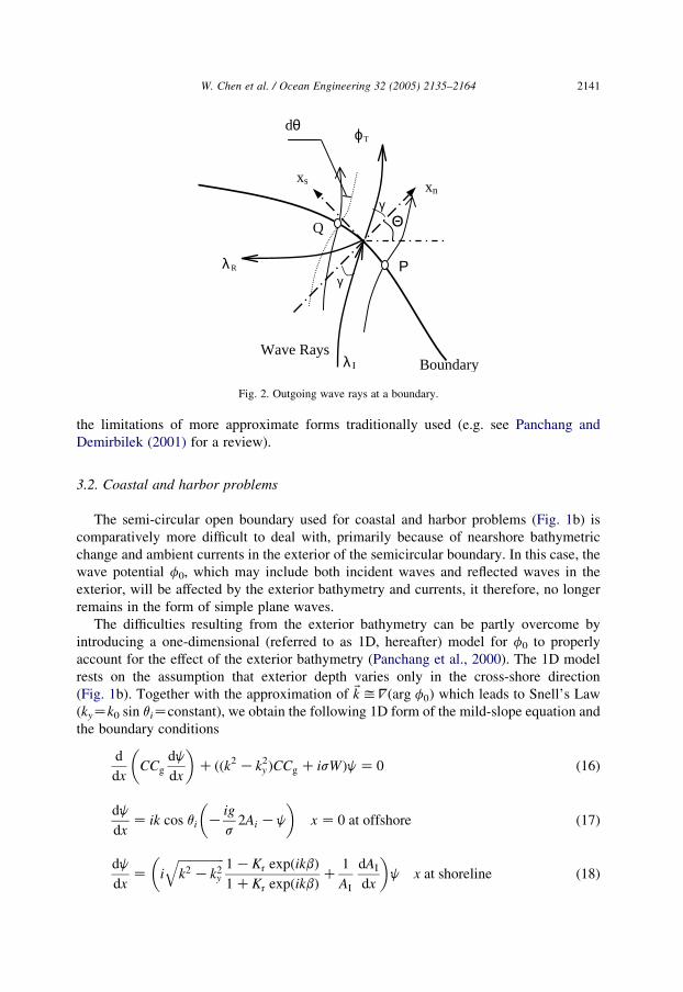
where as shown in Fig. 2, q is the approaching wave direction accounting for both wave

incident angle g and boundary orientation angle Q, such that qZQCg. The two terms on

the right-hand side of (15a) represent, respectively, the effects of wave convergence or

divergence and bathymetric change. It is noted that (15a) does not account for the energy

dissipation, and so it is invalid if waves were to break before reaching the boundary

(shoreline). In that event, though, (15a) becomes insignificant and can simply be

neglected.

Eq. (15) is nonlinear in the sense that the wave angle g is a function of the unknown f.

Most conventional wave models have in practice neglected the outgoing wave angle by

setting gZ0. This often results in spurious effects, while simulating wave transformation

in harbors or jettied inlets (Isaacson and Qu, 1990; Beltrami et al., 2001; Chen et al., 2002).

Further, as demonstrated by Chen et al. (2002), (15a) eliminates spurious reflections

arising from boundary curvature and the depth cut-off at shoreline boundaries (since

zero depth is not allowed). The boundary condition (15) can, therefore, overcome

d

P

Q

xs xn

ϕT

γ

γ

λ I

λ R

BoundaryWave Rays

Θ

θ

Fig. 2. Outgoing wave rays at a boundary.


the limitations of more approximate forms traditionally used (e.g. see Panchang and

Demirbilek (2001) for a review).

3.2. Coastal and harbor problems

The semi-circular open boundary used for coastal and harbor problems (Fig. 1b) is

comparatively more difficult to deal with, primarily because of nearshore bathymetric

change and ambient currents in the exterior of the semicircular boundary. In this case, the

wave potential f0, which may include both incident waves and reflected waves in the

exterior, will be affected by the exterior bathymetry and currents, it therefore, no longer

remains in the form of simple plane waves.

The difficulties resulting from the exterior bathymetry can be partly overcome by

introducing a one-dimensional (referred to as 1D, hereafter) model for f0 to properly

account for the effect of the exterior bathymetry (Panchang et al., 2000). The 1D model

rests on the assumption that exterior depth varies only in the cross-shore direction

(Fig. 1b). Together with the approximation of ðk yVðarg f0Þ which leads to Snell’s Law

(kyZk0 sin qiZconstant), we obtain the following 1D form of the mild-slope equation and

the boundary conditions

d

dxCCg

dj

dx

� �C ððk2 Kk2

y ÞCCg C isWÞj Z 0 (16)

dj

dxZ ik cos qi K

ig

s2Ai Kj

� �x Z 0 at offshore (17)

dj

dxZ i

ffiffiffiffiffiffiffiffiffiffiffiffiffiffiffik2 Kk2

y

q1 KKr expðikbÞ

1 CKr expðikbÞC

1

AI

dAI

dx

� �j x at shoreline (18)


where the second term in (18) may be neglected if wave breaking occurs, before waves

reach the boundary, otherwise it is given by

1

AI

vAI

vxZK

1

2Cg

vCg

vx(18a)

In Eqs. (16)–(18), the variable j is related to f0 by

f0 Z jðxÞexpðikyyÞ (19)

where (x, y) refers to a coordinate system shown in Fig. 1b, with the incident wave

condition specified at the origin, the offshore end of the 1D transect.

In practical applications, two 1D solutions j1 and j2 may be sought to account for the

bathymetry differences between two sides of the semicircular open boundary. To obtain f0

along the boundary, the two solutions are further interpolated and mapped onto the

boundary as

f0 Z1 Cy=R

2j1ðxÞC

1 Ky=R

2j2ðxÞ

� �expðikyyÞ (20)

where R is the radius of the semicircular boundary.

While the above treatment has been shown to effectively handle the problem of the

bathymetric variations in the exterior (Panchang et al., 2000; Zhao et al., 2000; Panchang

and Demirbilek, 2001), the problem of varying ambient currents in the exterior is more

challenging and has no standard solution yet. If the current field were to vary only in the x

(cross-shore) direction in the exterior, i.e. ðU Z ðuðxÞ; vðxÞÞ, its effect may be incorporated

into the 1D model for the solution of f0. However, such a current field is rare in practice

and we perforce assume that the effect of ambient currents on incident waves is negligible

in the exterior region. Diligence should be exercised in selecting the model domain and in

specifying f0.

For the scattered waves, depth variations that occur along the semicircular boundary

may render the parabolic condition (12) inappropriate (Panchang et al., 2000); a simple

expression for q as in (13) cannot be obtained. In such a case, the lower-order absorbing

boundary condition (15) that incorporates the incident angle would be more applicable.

Because the open boundary is fully transmitting (KrZ0), fs along this boundary may be

written as

vfs

vxn

Z ik cos g Kvq

2vxs

K1

2Cg

vCg

vxn

� �fs (21)

It is noted that, in cases, where the bottom slope is mild and scatterers are weak and

originate from near the center of a large semicircle, (21) can be effectively simplified as

vfs

vxn

Z ik K1

2R

� �fs (22)

which is the same form used by Panchang et al. (2000).


The overall open boundary condition for f is then

vf

vxn

Z ik K1

2R

� �ðf Kf0ÞC

vf0

vxn

(23)

where quantities related to f0 are obtained from (19) or (20).

The coastal boundary condition for coastal/harbor problems is the same as that for open

sea problems, and is given by (15).

4. Numerical implementation

Eq. (8) together with the dispersion relations and the appropriate boundary conditions

as described above forms a formidable boundary value problem from the viewpoint of

numerical implementation. Nonlinearities are encountered in the governing equations

(wave–current interaction and wave breaking) and in the boundary conditions (when the

direction-related expressions are employed). Nonlinear mechanisms can only be treated in

an iterative manner, allowing the boundary value problem to be linearized and solved

during each iteration by means of the finite-element method. Three aspects of the

numerical implementation are discussed below.

4.1. Determination of nonlinear parameters

4.1.1. Wave direction and Doppler shift

The effect of current-induced Doppler shift is incorporated into the kinematic

parameters k and s through the combined dispersion relations (2) and (3) or (5) and (3). To

determine the parameters k and s, it is necessary to first calculate the wave direction. Wave

direction is traditionally obtained from the phase gradient, which is

Vðarg fÞ Z VðImðln fÞÞ Z ImðVf=fÞ (24)

therefore, the wave direction q is determined by,

tan q Zvðarg fÞ

vy

�vðarg fÞ

vxZ Im

1

f

vf

vy

� ��Im

1

f

vf

vx

� �(25)

Taking q as the direction of vector ðk, the Doppler shift relation (3) can then be

re-written as

s Z u Kkðu cos q Cv sin qÞ (26)

Once q is known the intrinsic frequency s and the Doppler shifted wave number k may

be obtained by solving the combined nonlinear Eqs. (2) and (26), or (5) and (26) if one uses

the nonlinear dispersion relation.

It is noted that wave direction can be defined only in a wave field that is mainly

progressive. In some harbor areas, the wave field f may contain multi-directional wave

components due to wave scattering and reflection. The wave direction obtained from (25)

may then be viewed as the primary direction of wave propagation. Since the parameters


k and s are calculated on the basis of this wave direction, the effect of currents (Doppler

shift) on scattered waves moving in other directions cannot be correctly accounted for by

using these parameters. Strictly speaking, in a combined wave–current environment, wave

kinematics and the flowfield dynamics are coupled and cannot be solved separately. If the

wave field is dominated by waves that have readily identifiable directions, the effect of

currents on other (weak) wave components would remain small so as not to significantly

affect the accuracy of modeling results. This is true because the scattered field is generally

weak when there is no significant wave reflection from coastal boundaries. In case of

strong coastal reflection, we have to assume that reflected waves do not ride through the

major current field in directions largely collinear with flow directions. Otherwise the

reflected wave field must be treated separately from the forward-propagating wave field.

This aspect remains a topic of further research.

4.1.2. Outgoing wave angle at a boundary

The absorbing boundary conditions (15) and (21) require knowledge of g, the incident

wave angle relative to the normal direction at the boundary. For scattered waves at the

offshore open boundary, this angle can be determined in a manner similar to (25) with

tan g Zvðarg fsÞ

vxs

�vðarg fsÞ

vxn

(27)

At a coastal boundary, however, as noted in Section 3, approaching waves may be

partially reflected. In the presence of reflected waves, (25) cannot be used to find g because

of the multi-directionality in the wave potential f. Considering the combination of

incident and reflected waves, Chen et al. (2002) and Steward and Panchang (2001) have

developed the following equation for determining the approaching wave direction and

demonstrated its robustness for use in nonlinear calculations,

tan g Zð1 KK2

r Þ

1 C2Kr cosðkbÞCK2r

vðarg fÞ

vxs

�vðarg fÞ

vxn

(28)

Note that (28) reverts to (27) when boundary has zero reflection (KrZ0), and (27)

reverts to (25) if x and y were used instead of xn and xs. (28) may present difficulties when

v(arg f)/vxn and v(arg f)/vxs are both nearly zero. This implies a situation with standing

waves, which eliminates the need for an establishing g for use in (15).

4.1.3. Breaking parameter W

A number of formulations for the wave breaking parameter W can be found in the

literature, but few of them have been well-tested in an environment with strong wave–

current interaction. In the absence of wave–current interaction, Zhao et al. (2000)

examined five different parameterizations for W and concluded that the formulations of

Battjes and Janssen (1978) and Dally et al. (1985) are the most robust for use with the

mild-slope wave equation. Later, Zubier et al. (2003) indicated that the formulation of

Battjes and Janssen (1978) provides a better fit to field data than that of Dally et al. (1985).

We therefore use, in this work, the breaking criterion of Battjes and Janssen (1978), which

has also been used by Booij et al. (1999) in their energy-balance wave model.


4.2. Finite element formulation and solution of linear systems

The flexibility afforded by the choice of finite elements not only permits the best fit to

arbitrarily-shaped boundaries, but also provides the most efficiency in grid generation.

Locally wavelength-dependent grids (with a typical resolution of 15–20 grids per

wavelength) of varying size can be used, hence keeping the number of grids to an

optimum. (The finite-difference method, on the other hand, requires an excessive number

of grids since the size would be limited based on the shallowest depths; this compounds the

computational difficulties). We used a graphics software package called the Surface Water

Modeling System (Zundel et al., 1998) to construct a network of triangular finite elements.

With the inclusion of wave–current interaction, the governing Eq. (8) becomes more

complicated, requiring in the finite-element formulation use of the more general

variational principle (Galerkin approach), rather than the Jacobian functional method

used by Xu et al. (1996). For each of the n nodes in the discretized domain, a linear

weighting function is chosen on basis of local triangular meshes. Integration of (8) in

accordance with the Galerkin principle leads to a large sparse linear system

½K� ffg Z ffg (29)

where [K] is the n!n stiffness matrix, {f} the load vector, and {f} the solution vector of

unknowns fi (iZ1,2,.,n). Details of derivation may be found in Chen, 2002).

As in the case without ambient current, (29) forms an extremely large (n is typically at

an order of 105) complex-valued system. Without ambient currents, Panchang et al. (1991)

solved (29) by applying a pre-conditioned conjugate gradient iterative scheme to the

normalized equation. Several other iterative methods have since been used with varying

success (Li, 1994; Oliveira and Anastasiou, 1998). The iterative scheme of Li (1994) is

probably the most efficient algorithm for solving the symmetric linear system resulting

from the mild-slope equation or its variants without currents. However, when currents are

included, the stiffness matrix [K] is no longer symmetric or Hermitian, as a result of the

additional term ðU$Vf in (8). We found that Li’s algorithm then does not lead to

convergence. Even the stabilized biconjugate method (BiCGStab, Van der Vorst, 1992),

originally developed for solving nonsymmetric systems, failed to yield a converged

solution for some of the test cases presented in the next section. It is concluded based on

our testing that, for a nonsymmetric and non-Hermitian complex-valued linear system

associated with (8), the algorithm of Panchang et al. (1991) is probably the most robust and

guaranteed to converge.

4.3. Iterative scheme for multiple nonlinear mechanisms

As noted earlier, the parameters k, s, W and g are nonlinear and have to be solved,

together with f, by iteration. In an iterative scheme, these nonlinear parameters are pre-

determined based on the solution of f from the previous iteration step, so that a new linear

system for f can be formed based on the finite-element method and solved as discussed

above. The first linear solution f may be obtained by assuming zero currents (UZ0), no

breaking (WZ0), and gZ0. The nonlinear iterations proceed until the following stopping


criterion is met:

MaximumiZ1;n

jjfijj K jfijjK1j=jfincj!3 (30)

where i is the node number, j the number of iterations, jfincj the amplitude of the incident

wave potential at offshore (xZ0), and 3 is a pre-specified tolerance (typically 3Z10K3).

Since jfincj is a fixed reference value for all nodes, (30) actually defines the maximum

tolerable absolute error (solution difference between two successive iterations) for the

entire domain.

The behavior of solution convergence is highly case-dependent, so termination may

require some judgment in adjusting the tolerance level 3, or even the use of different

stopping criteria. In iterative methods, a very common approach is to use a relative error

(either maximum or average) for checking convergence. However, we found that using the

relative error imposed unnecessarily high accuracy on smaller waves in the breaking zone

while trying to maintain the desirable accuracy in the more prevalent non-breaking area.

Due to the dissipation term, iterative solutions in the breaking zone are more likely to

remain oscillating with small amplitudes, which could prevent convergence/model

termination. Our analysis indicated that using absolute error in the stopping criterion, as

given in (30), helps faster convergence without sacrificing the accuracy of solution in the

higher wave zones. It appears that (30) is a robust stopping criterion, capable of identifying

a reliable solution in general.

Iterative methods have been used for nonlinear mechanisms such as wave breaking (De

Girolamo et al., 1988; Zhao et al., 2000), wave direction-dependent boundary conditions

(Isaacson and Qu, 1990; Steward and Panchang, 2001; Beltrami et al., 2001), and wave–

current interaction (Kostense et al., 1988). There has been a concern that multiple

nonlinear mechanisms could slow down or even impede solution convergence. Our study

shows that multiple nonlinear parameters may be updated and iterated simultaneously

without difficulties in achieving convergence. This indicates that highly nonlinear wave–

current interaction problems can be solved effectively in such a manner.

5. Model validation

In this section, three cases of wave–current interaction of common interest are

simulated using the methods described above. The absence of data or analytical solutions

for typical cases of two-dimensional wave–current interaction precludes model validation

in the usual sense; however, the results are evaluated for overall consistency by comparing

them to the results of other models (either parabolic or Boussinesq time-dependent finite-

difference models).

5.1. Vortex ring

Vortex rings, commonly seen in open oceans and coastal seas, have important effects

on marine physical and biological processes (e.g. Mapp et al., 1985; Liu et al., 1994). The

complex wave patterns resulting from wave and vortex interaction can be captured by


airborne or satellite imagery. Liu et al. (1994) combined image processing and simple

wave modeling to identify the existence and strengths of underlying vortex rings. The

modeling procedure described here can be used as a more sophisticated alternative in

future studies of vortical flows and ocean gyres. Although this case can be easily tackled

using simpler parabolic approximation models, we describe it here for two reasons: (a) to

validate the code we developed before applying it to other cases, and (b) to highlight

certain features of the wave pattern that occur in more practical harbor engineering

problems discussed later (Section 6).

We consider the case of wave-vortex interaction studied by Mapp et al. (1985) and

Yoon and Liu (1989), who describe the current field as

Vr Z 0

Vq ZC5

rR1

� �N

r%R1

C6 exp K R2KrR3

� �2�

rRR1

8>><>>:

(31)

where Vr and Vq are the velocity components in polar coordinates with the origin at the

center of the ring. Following Yoon and Liu (1989), we set

C5 Z 0:9 m=s; C6 Z 1:0 m=s; N Z 2; R1 Z 343:706 m;

R2 Z 384:881 m; R3 Z 126:830 m:(32)

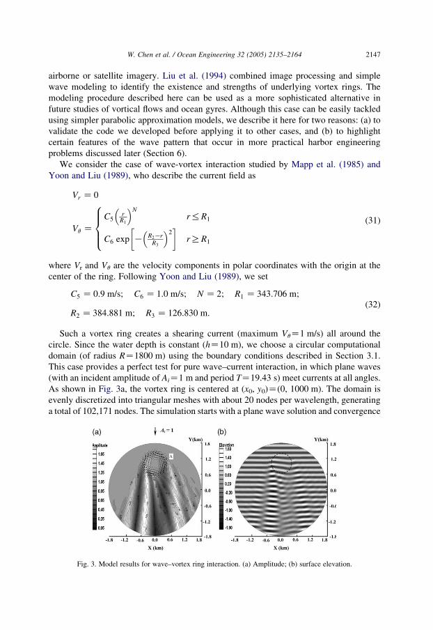
Such a vortex ring creates a shearing current (maximum VqZ1 m/s) all around the

circle. Since the water depth is constant (hZ10 m), we choose a circular computational

domain (of radius RZ1800 m) using the boundary conditions described in Section 3.1.

This case provides a perfect test for pure wave–current interaction, in which plane waves

(with an incident amplitude of AiZ1 m and period TZ19.43 s) meet currents at all angles.

As shown in Fig. 3a, the vortex ring is centered at (x0, y0)Z(0, 1000 m). The domain is

evenly discretized into triangular meshes with about 20 nodes per wavelength, generating

a total of 102,171 nodes. The simulation starts with a plane wave solution and convergence

Fig. 3. Model results for wave–vortex ring interaction. (a) Amplitude; (b) surface elevation.


is reached after only four nonlinear iterations for wave–current interaction. Wave breaking

is not activated in this case. The total run time for this simulation is about 15 min on a

2.4 GHz desktop PC.

The simulated wave amplitude and a snapshot of the surface elevation are presented in

Fig. 3. As can be seen, wave energy has been considerably redistributed due to the

disturbance created by the vortex ring. The effect of vortical flow on wave propagation is

complicated because progressive waves encounter shear currents at all angles. The vortex

ring not only affects the area, where opposing (left-hand side) and following (right-hand

side) currents exist, but also a large part of the down-wave region. The combined effect of

wave refraction, diffraction, and reflection give rise to modulations of wave amplitude that

are neither symmetric nor regularly oriented.

Yoon and Liu (1989) modeled this problem with a finite-difference, phase-resolving,

parabolic approximation. The overall wave pattern obtained by them (Fig. 13a in Yoon

and Liu, 1989) is similar to ours (Fig. 3a and b). Fig. 4 provides a detailed quantitative

comparison of the two model results for six lateral transects. Although the two models

agree well for this test case, it is noted that the method presented here has greater

versatility because it does not rely on the parabolic approximation. In fact, some

limitations of the parabolic approximation may be captured in Figs. 3 and 4. For instance,

due to the highly oblique angle with which waves approach the shearing current in the

vicinity of point A in Fig. 3a, wave caustics are expected to occur, causing a small band of

waves to be reflected toward the right (McKee, 1974; Peregrine and Smith, 1975). The

reflection is manifested in the form of amplitude modulations in our results (e.g. down-

wave and to the right of point A in Fig. 3, and to the right of B and C in Fig. 4). The

parabolic approximation model is not expected to simulate wave reflection or large-angle

diffraction, hence the model results of Yoon and Liu (1989) show a less disturbed solution

Y = 1765.70 m

0

1

2

A/A

i

Y = 1153.14 m

0

1

2

A/A

i

Y=540.58 m

0

1

2

A/A

i

Y= - 71.98 m

Y= - 684.53 m

Y= - 1297.09 m

X (km)

B

C

-1.5 0 1.5 -1.5 0 1.5X (km)

Fig. 4. Simulated relative wave amplitudes for wave–vortex ring interaction (thick line: present model; thin line:

Yoon and Liu (1989)).


to the right of B and C in Fig. 4. This type of reflection of waves that are obliquely incident

on a shearing current is relevant to our simulations pertaining to the interaction of waves

with tidal currents near an inlet (see Section 6.4).

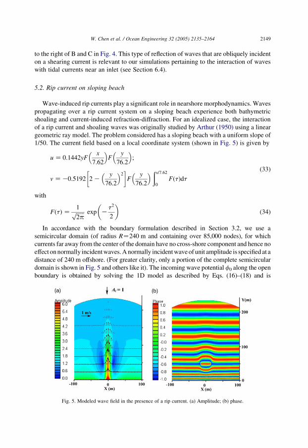
5.2. Rip current on sloping beach

Wave-induced rip currents play a significant role in nearshore morphodynamics. Waves

propagating over a rip current system on a sloping beach experience both bathymetric

shoaling and current-induced refraction-diffraction. For an idealized case, the interaction

of a rip current and shoaling waves was originally studied by Arthur (1950) using a linear

geometric ray model. The problem considered has a sloping beach with a uniform slope of

1/50. The current field based on a local coordinate system (shown in Fig. 5) is given by

u Z 0:1442yFx

7:62

� �F

y

76:2

� �;

v ZK0:5192 2 Ky

76:2

� �2�

Fy

76:2

� � ðx=7:62

0FðtÞdt

(33)

with

FðtÞ Z1ffiffiffiffiffiffi2p

p exp Kt2

2

� �(34)

In accordance with the boundary formulation described in Section 3.2, we use a

semicircular domain (of radius RZ240 m and containing over 85,000 nodes), for which

currents far away from the center of the domain have no cross-shore component and hence no

effect on normally incident waves. A normally incident wave of unit amplitude is specified at a

distance of 240 m offshore. (For greater clarity, only a portion of the complete semicircular

domain is shown in Fig. 5 and others like it). The incoming wave potential f0 along the open

boundary is obtained by solving the 1D model as described by Eqs. (16)–(18) and is

Fig. 5. Modeled wave field in the presence of a rip current. (a) Amplitude; (b) phase.

T = 8s

0

2

4

6

8

10

A/A

i

Improved BC

Conventional BC

T= 16s

0

2

4

6

8

10

X = 0

X = 0

X = 143.32 m X = 143.32 m

Y (m)0 20 40 60 80 0 20 40 60 80

Y (m)

Fig. 6. Simulated relative wave amplitudes using two boundary conditions.


substituted into (23) to obtain the open boundary condition for the 2D model. Wave breaking

is not activated for consistency with other model results (e.g. Yoon and Liu, 1989).

To avoid the singularity of zero depth at the coastline, we place the shoreline boundary

at yZ1 m, where the cut-off depth is 0.02 m; it is specified as non-reflective boundary

(KrZ0, bZ0) using generalized boundary condition (15). Because of the large shoaling

effect near the shoreline, the second term in (15) plays an important role. This can be seen

in Fig. 6, where results for simulations with two different incident wave periods are shown.

The improved boundary condition (15) is effective in eliminating spurious reflections

resulting from the cut-off depth at the shoreline. These spurious reflections are seen quite

significant for longer waves, even with a very mild bottom slope (1/50) in this case.

The model simulation for TZ8 s in this case took five nonlinear iterations and about

10 min. Results shown in Fig. 5 indicate that the opposing rip current has modified the

wavelengths and caused a notable bending of phase contours. As a consequence, wave

energy is focused and trapped to form a high-wave zone along the centerline across shore;

this is accompanied by two symmetric shadow regions on the sides. The combined effects

of the rip current and bathymetric shoaling cause amplitude amplification to a factor over

six in the central area.

Our results are compared in Fig. 7 to the parabolic approximation results of Yoon and

Liu (1989) along four longshore and two cross-shore transects, and again fairly good

agreement is seen in general. However, there is an obvious mismatch along xZ0 for

y!60 m. Our results show that the amplitude has a peak value of 5.5 at approximately

45 m offshore, and after a small drop, it increases to about 10 at the boundary. In other

words, the non-breaking amplitude has nearly doubled in the shallowest 25 m of the

domain, where opposing current is becoming negligible. The results of Yoon and Liu

(1989), on the other hand, show a significant drop from the peak value of 5 down to 3.2.

While using a different parabolic approximation, Liu (1983) speculated that this amplitude

drop was related to the lateral component of the current. We investigated this with

the elliptic finite-element model and found that suppressing the lateral velocity u made

Y=113.65 m

0

2

4

6A

/Ai

Y= 56.33 m

0

2

4

6

A/A

i

Y= 84.99 m

Y= 27.66 m

X = 0 m

0

2

4

6

A/A

i

0 60 120 180 240 0 60 120 180 240

Y (m)Y (m)

0 25 50 75 100 0 25 50 75 100X (m) X (m)

X = 143.32 m

Fig. 7. Simulated relative wave amplitudes, rip current case (thick line: present model; thin line: Yoon and Liu,

1989).


little difference. On the other hand, it may be noted that shoaling alone causes a similar

doubling at other cross-shore transects (e.g. xZ143.34 m). We submit, therefore, that the

increase in the amplification obtained by the elliptic model is a reasonable feature that the

parabolic approximation cannot capture. Parabolic approximations assume that the second

derivative of wave amplitude in the dominant wave propagation direction is of higher-

order and hence dropped; in this case, the assumption may not be appropriate. The

mismatch between the parabolic approximations and elliptic equation solutions (Fig. 7)

are significant only near the central nearshore area or around the shadow areas (xyG15 m), where wave amplitudes apparently experience considerable change in the x

direction. At distant cross-shore sections, the two models agree because changes in the

x-direction are less enhanced.

5.3. Rip current on beach with sandbar

We consider a second, more realistic, rip current case that has been studied by Chen

et al. (1999). Fig. 8 shows the bathymetry of a plane beach with a discontinuous offshore

sandbar and the underlying rip current field. The current field, provided to us by Professor

Q. Chen of the University of South Alabama, is more complicated than that in Section 5.2.

Strong vorticity characterizes much of the current field, for instance, on both sides of

the central jet of the rip current and also behind the sandbar in the surf zone. The vortices

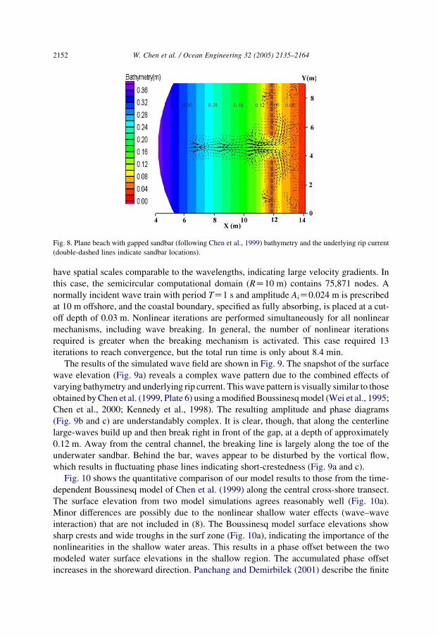
Fig. 8. Plane beach with gapped sandbar (following Chen et al., 1999) bathymetry and the underlying rip current

(double-dashed lines indicate sandbar locations).


have spatial scales comparable to the wavelengths, indicating large velocity gradients. In

this case, the semicircular computational domain (RZ10 m) contains 75,871 nodes. A

normally incident wave train with period TZ1 s and amplitude AiZ0.024 m is prescribed

at 10 m offshore, and the coastal boundary, specified as fully absorbing, is placed at a cut-

off depth of 0.03 m. Nonlinear iterations are performed simultaneously for all nonlinear

mechanisms, including wave breaking. In general, the number of nonlinear iterations

required is greater when the breaking mechanism is activated. This case required 13

iterations to reach convergence, but the total run time is only about 8.4 min.

The results of the simulated wave field are shown in Fig. 9. The snapshot of the surface

wave elevation (Fig. 9a) reveals a complex wave pattern due to the combined effects of

varying bathymetry and underlying rip current. This wave pattern is visually similar to those

obtained by Chen et al. (1999, Plate 6) using a modified Boussinesq model (Wei et al., 1995;

Chen et al., 2000; Kennedy et al., 1998). The resulting amplitude and phase diagrams

(Fig. 9b and c) are understandably complex. It is clear, though, that along the centerline

large-waves build up and then break right in front of the gap, at a depth of approximately

0.12 m. Away from the central channel, the breaking line is largely along the toe of the

underwater sandbar. Behind the bar, waves appear to be disturbed by the vortical flow,

which results in fluctuating phase lines indicating short-crestedness (Fig. 9a and c).

Fig. 10 shows the quantitative comparison of our model results to those from the time-

dependent Boussinesq model of Chen et al. (1999) along the central cross-shore transect.

The surface elevation from two model simulations agrees reasonably well (Fig. 10a).

Minor differences are possibly due to the nonlinear shallow water effects (wave–wave

interaction) that are not included in (8). The Boussinesq model surface elevations show

sharp crests and wide troughs in the surf zone (Fig. 10a), indicating the importance of the

nonlinearities in the shallow water areas. This results in a phase offset between the two

modeled water surface elevations in the shallow region. The accumulated phase offset

increases in the shoreward direction. Panchang and Demirbilek (2001) describe the finite

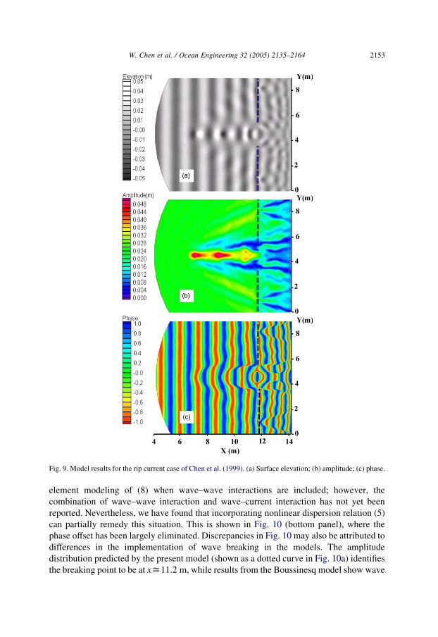
Fig. 9. Model results for the rip current case of Chen et al. (1999). (a) Surface elevation; (b) amplitude; (c) phase.


element modeling of (8) when wave–wave interactions are included; however, the

combination of wave–wave interaction and wave–current interaction has not yet been

reported. Nevertheless, we have found that incorporating nonlinear dispersion relation (5)

can partially remedy this situation. This is shown in Fig. 10 (bottom panel), where the

phase offset has been largely eliminated. Discrepancies in Fig. 10 may also be attributed to

differences in the implementation of wave breaking in the models. The amplitude

distribution predicted by the present model (shown as a dotted curve in Fig. 10a) identifies

the breaking point to be at xy11.2 m, while results from the Boussinesq model show wave

(a)

Y = 4.55 m

-0.06

0

0.06

0.12

10 12 14

Ele

vatio

n (m

)

-0.06

0

0.06

0.12

Ele

vatio

n (m

)

Linear ModelChen et al. (1999)

Y = 4.55 mWeak-Nonlinear ModelChenet al. (1999)Amplitude

(b)

4 6 8X (m)

10 12 144 6 8X (m)

Amplitude

Fig. 10. Simulations of the rip current case of Chen et al. (1999).


heights decreasing only after xy12 m. The absence of benchmark data is a handicap

preventing us from further verifying the breaking criteria used the two models.

6. Wave pattern near a jettied tidal inlet

The effect of tidal currents on wave propagation near an entrance to a harbor is a

problem of interest in coastal engineering practice since it affects navigation safety, inlet

entrance maintenance, jetty design, harbor performance, etc. Smith et al. (1998) conducted

a laboratory study to investigate the wave–current interaction and the associated wave

breaking in the presence of ebb currents in an idealized entrance. We use this case as an

example to develop an understanding of the wave patterns that may be expected in such

configurations. Since the hydraulic model measurements for waves, currents, and

bathymetry were not detailed enough for a systematic model validation, a comparison can

be performed only in a general sense. However, the comparison is sufficiently satisfactory

and the numerical results are sufficiently informative (in fact, they shed more light on the

phenomena than the laboratory data do) that they provide the motivation to supplement the

hydraulic model study with numerical investigations of additional conditions of interest in

this harbor engineering problem.

6.1. Summary of hydraulic model data

Fig. 11 (Smith et al., 1998) shows the overall arrangement of the physical model facility

built at a prototype scale of 1:50. A wave maker is situated 24 m offshore at the head of

Fig. 11. Hydraulic model layout, idealized inlet facility (after Smith et al., 1998).


the model basin and currents can be generated by a pumping system. Fig. 12 shows the

detailed geometry and bottom topography in the vicinity of the jettied inlet, where model

simulations are focused. The idealized bathymetry is based on the design data for physical

model construction. Most of the domain consists of a beach that slopes down to a depth of

about 0.2 m, followed by a steep-slope leading to the deepwater end, where water depth is

constant. Two parallel jetties are built to create an entrance channel, between which the

depth is constant. This is preceded by a deep trench at the throat, which connects the backbay

area (harbor) to the entrance channel. Experiments were limited to normally incident waves

and ebb currents. Wave heights, currents, and water depths were measured at six gauges

(Fig. 12) along the main channel. Laboratory runs were made using narrow-band

unidirectional waves with desired target significant wave heights and peak periods. These

are simulated numerically using a monochromatic representation with the associated

significant wave heights and peak periods. This assumes that narrow-band unidirectional

seas can be reasonably approximated by the equivalent monochromatic waves.

Fig. 12. Wave model domain, detailed bathymetry (depth in m), and underlying ebb current. Circles indicate

gauge locations numbered from one at offshore to six near the inlet.


6.2. Flowfield simulation

A detailed current field was not available from hydraulic model study since

measurements were made only at the locations shown in Fig. 12. A synthetic flow field

had to be generated numerically to approximate the actual flow conditions in the

laboratory. The two-dimensional circulation model DUCHESS, developed at TU Delft

(Booij, 1989; Jin and Kranenburg 1993) was applied to a domain extending G30 m in the

longshore direction and 30 m to the offshore direction, large enough to minimize any

potential adverse lateral open boundary effects. The backbay area is not of interest for this

study and was eliminated by placing a water boundary at the inlet throat (yZK4 m). The

volume flux along this boundary with certain distribution was prescribed to drive the

model for desired ebb-flow field. All offshore model boundaries are treated as flow-

through (non-reflecting) using a radiation boundary condition. To prevent instabilities in

the model solution, the volume flux was ramped up gradually from zero to a specified

value, and was maintained constant, thereafter, until the current field in the entire

modeling domain reached equilibrium. Input volume flux (which is unavailable from the

hydraulic model data), bottom friction, and eddy viscosity were used as calibration

coefficients in order to obtain the best fit between simulated currents and the data observed

at the gauges.

The resulting jet-like ebb current field from model simulation is shown in Fig. 12. (For

clarity, only a part of the flow model domain is shown). Detailed velocity profiles are

provided in Fig. 13a along four transects across the mainstream of the ebb flow. The

velocity distributions show a common structure of double-peak shear currents, with the

shear structure intensifying from the offshore to a maximum near the middle of the throat,

and then decreasing as a result of the specified flowfield being constant. Fig. 13b shows the

variation of the current velocity along the centerline. A rapid change in velocity at near

yZ0 is due to the flow transition over a steep-slope from deep trench in the inlet throat to a

shallow flat area between the jetties. Also in Fig. 13b, the simulated currents are compared

to the measurements of two laboratory runs (Runs 3 and 4, described later) with the same

target flow conditions, showing apparently good agreement in both cases. However, it is

still uncertain how well the simulated current field represents the actual flow in the

laboratory study. In particular, the limited data prevent us from confirming the lateral

(shearing) structure of the ebb flow seen in Fig. 13a.

0

5

10

15

20

-5 10 15

Mode l resultsLab da ta - Run.3Lab da ta - Run.4

(a)

0

5

10

15

20y = 9 my = 5 my = 2 my =-3.25

X (m)

Vel

ocity

(cm

/s)

-6 -3 0 3 6 0 5Y (m)

x = 0(b)

Fig. 13. Simulated current velocity profiles. (a) Longshore transects; (b) cross-shore transect, compared to lab

data.


6.3. Simulation of normal wave incidence

We investigated two cases, without currents and with ebb currents, each of which consists

of a large-wave case and a small-wave case. The target significant incident wave amplitude is

2.75 cm for large-waves and 1.83 cm for small-waves in the laboratory study. The wave

period is 1.4 s for all cases. The computational domain for wave simulations, shown in Fig. 12,

consists of 165,371 triangular elements and 83,581 nodes (representing a resolution of 20

nodes per wavelength), and the radius of the semicircular boundary is 13.6 m. All shoreline

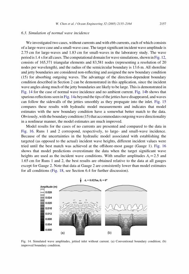
and jetty boundaries are considered non-reflecting and assigned the new boundary condition

(15) for absorbing outgoing waves. The advantage of the direction-dependent boundary

condition described in Section 2 can be demonstrated in this application, since the incident

wave angles along much of the jetty boundaries are likely to be large. This is demonstrated in

Fig. 14 for the case of normal wave incidence and no ambient current. Fig. 14b shows that

spurious reflections seen in Fig. 14a beyond the tips of the jetties have disappeared, and waves

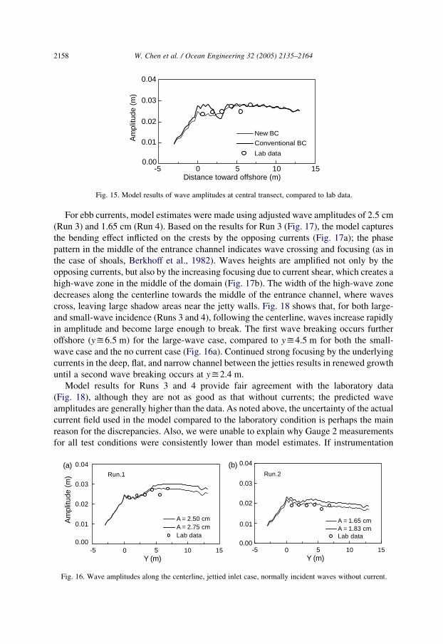
can follow the sidewalls of the jetties smoothly as they propagate into the inlet. Fig. 15

compares these results with hydraulic model measurements and indicates that model

estimates with the new boundary condition have a somewhat better match to the data.

Obviously, with the boundary condition (15) that accommodates outgoing wave directionality

in a nonlinear manner, the model estimates are much improved.

Model results for the cases of no currents are presented and compared to the data in

Fig. 16. Runs 1 and 2 correspond, respectively, to large- and small-wave incidence.

Because of the uncertainties in the hydraulic model associated with establishing the

targeted (as opposed to the actual) incident wave heights, different incident values were

tried until the best match was achieved at the offshore-most gauge (Gauge 1). Fig. 16

shows that model predictions overestimate the data when the target significant wave

heights are used as the incident wave conditions. With smaller amplitudes AiZ2.5 and

1.65 cm for Runs 1 and 2, the best results are obtained relative to the data at all gauges

except for Gauge 2. Note that data at Gauge 2 are consistently lower than model estimates

for all conditions (Fig. 18, see Section 6.4 for further discussion).

Fig. 14. Simulated wave amplitudes, jettied inlet without current. (a) Conventional boundary condition; (b)

improved boundary condition.

0.01

0.00

0.02

0.03

0.04

Am

plitu

de (

m)

New BC

Conventional BC

Lab data

Distance toward offshore (m)-5 0 5 10 15

Fig. 15. Model results of wave amplitudes at central transect, compared to lab data.


For ebb currents, model estimates were made using adjusted wave amplitudes of 2.5 cm

(Run 3) and 1.65 cm (Run 4). Based on the results for Run 3 (Fig. 17), the model captures

the bending effect inflicted on the crests by the opposing currents (Fig. 17a); the phase

pattern in the middle of the entrance channel indicates wave crossing and focusing (as in

the case of shoals, Berkhoff et al., 1982). Waves heights are amplified not only by the

opposing currents, but also by the increasing focusing due to current shear, which creates a

high-wave zone in the middle of the domain (Fig. 17b). The width of the high-wave zone

decreases along the centerline towards the middle of the entrance channel, where waves

cross, leaving large shadow areas near the jetty walls. Fig. 18 shows that, for both large-

and small-wave incidence (Runs 3 and 4), following the centerline, waves increase rapidly

in amplitude and become large enough to break. The first wave breaking occurs further

offshore (yy6.5 m) for the large-wave case, compared to yy4.5 m for both the small-

wave case and the no current case (Fig. 16a). Continued strong focusing by the underlying

currents in the deep, flat, and narrow channel between the jetties results in renewed growth

until a second wave breaking occurs at yy2.4 m.

Model results for Runs 3 and 4 provide fair agreement with the laboratory data

(Fig. 18), although they are not as good as that without currents; the predicted wave

amplitudes are generally higher than the data. As noted above, the uncertainty of the actual

current field used in the model compared to the laboratory condition is perhaps the main

reason for the discrepancies. Also, we were unable to explain why Gauge 2 measurements

for all test conditions were consistently lower than model estimates. If instrumentation

Run.2

0.00

0.01

0.02

0.03

0.04

-5 10 15

A = 1.65 cmA = 1.83 cmLab data

(a) Run.1

0.00

0.01

0.02

0.03

0.04

A = 2.50 cm A = 2.75 cm Lab data

Am

plitu

de (

m)

0 5Y (m)

-5 10 150 5Y (m)

(b)

Fig. 16. Wave amplitudes along the centerline, jettied inlet case, normally incident waves without current.

Fig. 17. Model results for a jettied inlet case, with ebb current. (a) Phase; (b) amplitude.


errors were involved at this gauge, we would have lost important information about the

onset of wave breaking. Yet, as Fig. 17 reveals, an intricate wave pattern may be expected

near harbor entrances with jetties; it also suggests, however, that many more

measurements would be needed to identify any meaningful features of the wave–current

interaction in the hydraulic model.

6.4. Oblique wave incidence

Since there are no data available for oblique wave incidence from the hydraulic model

study, we investigate the effect of ebb and flood currents on wave transformation. Fig. 19

shows numerical results for two simulations, i.e. for 458 incidence (AiZ2.5 cm)

0.00

0.01

0.02

0.03

0.04

-5 0 5 10 15

Am

plitu

de (

m)

A = 2.50 cmLab data, Run.3 A =1.65 cm Lab data, Run.4

Y (m)

Fig. 18. Wave amplitudes along the centerline, jettied inlet case; normal waves with ebb currents.

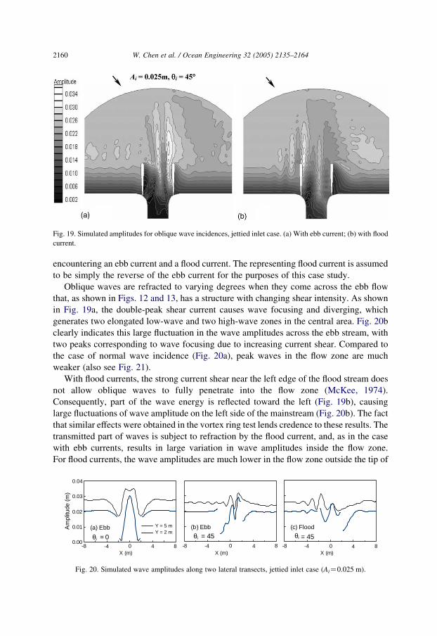
Fig. 19. Simulated amplitudes for oblique wave incidences, jettied inlet case. (a) With ebb current; (b) with flood

current.


encountering an ebb current and a flood current. The representing flood current is assumed

to be simply the reverse of the ebb current for the purposes of this case study.

Oblique waves are refracted to varying degrees when they come across the ebb flow

that, as shown in Figs. 12 and 13, has a structure with changing shear intensity. As shown

in Fig. 19a, the double-peak shear current causes wave focusing and diverging, which

generates two elongated low-wave and two high-wave zones in the central area. Fig. 20b

clearly indicates this large fluctuation in the wave amplitudes across the ebb stream, with

two peaks corresponding to wave focusing due to increasing current shear. Compared to

the case of normal wave incidence (Fig. 20a), peak waves in the flow zone are much

weaker (also see Fig. 21).

With flood currents, the strong current shear near the left edge of the flood stream does

not allow oblique waves to fully penetrate into the flow zone (McKee, 1974).

Consequently, part of the wave energy is reflected toward the left (Fig. 19b), causing

large fluctuations of wave amplitude on the left side of the mainstream (Fig. 20b). The fact

that similar effects were obtained in the vortex ring test lends credence to these results. The

transmitted part of waves is subject to refraction by the flood current, and, as in the case

with ebb currents, results in large variation in wave amplitudes inside the flow zone.

For flood currents, the wave amplitudes are much lower in the flow zone outside the tip of

(a) Ebb

0.00

0.01

0.02

0.03

0.04

Am

plitu

de (

m)

Y = 5 mY = 2 m

(b) Ebb

-8 -4 8

(c) Flood

-8 -4 8

θi = 0 θi = 45 θi = 45-8 -4 0 4 8 0 4 0 4

X (m) X (m) X (m)

Fig. 20. Simulated wave amplitudes along two lateral transects, jettied inlet case (AiZ0.025 m).

0.00

0.01

0.02

0.03

0.04

Y (m)

Am

plitu

de (

m)

Ebb,

Ebb, Flood,

θ i = 0˚˚

˚θ i = 45

θi = 45

-5 0 5 10 15

Fig. 21. Simulated wave amplitudes along the centerline, jettied inlet case (AiZ0.025 m).


jetties because of wave reflection at the left edge of the mainstream (Figs. 19b and 21) and

also because the waves are following the currents. In spite of this, more wave energy is

able to penetrate into the jetty channel and the inlet compared to the ebb current case,

either with normal or oblique incidence (Fig. 21). This is because flood currents have

turned the waves more toward the inlet, and that lower wave amplitudes have resulted in

less wave energy dissipation (breaking) in the channel and inlet area between jetties.

7. Concluding remarks

We have provided a comprehensive treatment of the various issues associated with

finite-element modeling of the elliptic wave–current interaction equation. Methods to

effectively handle various nonlinear aspects of the solution are developed. Implementation

of an improved boundary absorption condition that accounts for the angle of wave

approach and the local bathymetric variation has largely eliminated the spurious

oscillations commonly seen in the solutions of similar models. The model developed on

the basis of the methods detailed here was applied to three wave–current interaction cases.

The results were found to be consistent with those of other published models.

Relative to the frequently used parabolic approximation models (e.g. Yoon and Liu,

1989), the present results are nearly identical in some cases. In other cases, the limitations

of the parabolic approximations are illustrated, such as the effect of dropping the second-

order derivative when the wave height changes rapidly (as in the rip-current test-case).

Also, the reflective pattern seen in the elliptic model results as a consequence of a highly

oblique angle at which waves approach the current field permits one to speculate that

parabolic approximations may be inadequate in the case of strong velocity shears, where

large-angle wave refraction, diffraction, and even reflection (due to wave caustics) may be

expected. Relative to Boussinesq models, which have traditionally been applicable only to

shallow water waves1 the present approach suffers, in principle, from the disadvantage of

inadequate representation of nonlinear shallow-water effects. However, the results

obtained here show only minor discrepancies, and even those are somewhat diminished

1 The applicability of Boussinesq models is now being extended to intermediate and deep water depths.


through the use of the nonlinear dispersion relation (5). Also, a strategy for including

wave–wave interactions in elliptic finite element models and some preliminary results

have been described in Panchang and Demirbilek (2001). Since multiple nonlinear

mechanisms have been successfully handled in the work reported here, incorporating the

additional mechanism of wave–wave interaction may not be problematic. Further, a finite-

element formulation that can better represent complex geometries (such as the case of

jettied inlets) is more conducive to the time-independent elliptic formulation (8) than to

the time-dependent and highly nonlinear Boussinesq models.

The satisfactory solutions obtained for the tests described in Section 5 prompted the

investigation of wave–current interactions near a jettied tidal inlet, a problem of

considerable engineering importance (e.g. Lin and Demirbilek, in press; Smith et al.,

1998). The wave patterns are seen to be quite intricate. Ebb currents lead to considerable

breaking outside the entrance channel, but renewed wave growth occurs due to focusing by

the currents before the waves break again. For flood tides, the wave heights are smaller

outside the jetty channel, as a consequence of the non-opposing nature of the waves and

currents, but they are larger than in the ebb current case inside the channel because waves

do not break. Although the case investigated here dealt with the layout constructed by

Smith et al. (1998), the overall results presented here have set the stage for tackling

practical engineering problems.

The solution methods proposed here require only moderate computer power. The

examples illustrated show that a typical application involving monochromatic wave

transformation would take about 15 min of run time on a modern PC.

Acknowledgements

Partial support for this work was received from the Office of Naval Research, the Army

Corps of Engineers, the Maine Sea Grant Program, and the National Sea Grant Office. We

are grateful to Professor Q. Chen of the University of South Alabama for providing the

flow field for one of the rip current cases investigated. Assistance provided by Messrs K.

Schlenker, K. Zubier, and L. Zhao is acknowledged.

References

Arthur, R.S., 1950. Refraction of shallow water waves: the combined effect of currents and under water

topography. EOS Trans. 31, 549–552.

Battjes, J.A., Janssen, J., 1978. Energy loss and set-up due to breaking of random waves, Proceedings of the 16th

International Conference Coastal Engineering. ASCE, New York, pp. 569–587.

Beltrami, G.M., Bellotti, G., De Girolamo, P., Sammarco, P., 2001. Treatment of wave breaking and total

absorption in a mild-slope equation FEM model. J. Waterw., Port, Coastal Ocean Eng. 127, 263–271.

Berkhoff, J.C.W., 1972. Computation of combined refraction and diffraction, Proceedings of the 13th

International Conference Coastal Engineering. ASCE, New York.

Berkhoff, J.C.W., Booy, N., Radder, A.C., 1982. Verification of numerical wave propagation models for simple

harmonic linear water waves. Coastal Eng. 6, 255–279.


Booij, N., 1981. Gravity waves on water with non-uniform depth and current. Technical Report 81-1, Department

of Civil Enging, Delft University of Technology, The Netherlands.

Booij, N., 1989. User manual for the program DUCHESS. Technical Report, Delft University of Technology, The

Netherlands.

Booij, N., Ris, R.C., Holthuijsen, L.H., 1999. A third-generation wave model for coastal regions. 1. Model

description and validation. J. Geophys. Res. 104 (c4), 7649–7666.

Chamberlain, P.G., Porter, D., 1995. The modified mild-slope equation. J. Fluid Mech. 291, 393–407.

Chen, W., 2002. Finite element modeling of wave transformation in harbors and coastal regions with complex

bathymetry and ambient currents. PhD dissertation, Department of Civil Engineering, University of Maine,

Orono. USA.

Chen, Q., Darlrymple, R.A., Kirby, J.T., Kennedy, A.B., Haller, M.C., 1999. Boussinesq modeling of a rip current

system. J. Geophys. Res. 104 (c9), 20617–20637.

Chen, W., Panchang, V.G., Demirbilek, Z., 2002. A generalized absorbing boundary condition for elliptic harbor

wave models, Proceedings of the 4th International Symposium on Ocean Wave Measurement and Analysis,

vol. 1. ASCE, New York, pp. 714–723.

Dally, W.R., Dean, R.G., Dalrymple, R.A., 1985. Wave height variation across beaches of arbitrary profile.

J. Geophys. Res. 90 (c6), 11917–11927.

De Girolamo, P., Kostense, J.K., Dingemans, M.W., 1988. Inclusion of wave breaking in a mild-slope model. In:

Schrefler, Zienkiewicz (Eds.), Computer Modeling in Ocean Engineering. Balkema, Rotterdam, pp. 221–229.

Grassa, J.M., Flores, J., 2001. Discussion of: ‘Maa, J.P.-Y.; Hsu, T.-W.; Tsai, C.H., Juang, W.J., 2000.

Comparison of Wave Refraction and Diffraction Models’. J. Coastal Res. 17 (3), 762.

Isaacson, M., Qu, S., 1990. Waves in a harbour with partially reflecting boundaries. Coastal Eng. 14, 193–214.

Kirby, J.T., 1984. A note on linear surface wave–current interaction over slowly varying topography. J. Geophys.

Res. 89 (c1), 745–747.

Kirby, J.T., 1989. A note on parabolic radiation boundary conditions for elliptic wave calculation. Coastal Eng.

13, 211–218.

Kirby, J.T., Dalrymple, R.A., 1986. An approximate model for nonlinear dispersion in monochromatic wave

propagation models. Coastal Eng., 9, 545–561.

Kirby, J.T., Dalrymple, R.A., 1994. Combined refraction/diffraction model REF/DEF 1, version 2.5,

documentation and user’s manual. Research Report No. CACR-94-22, Department of Civil Engineering,

University of Delaware.

Kostense, J.K., Dingemans, M.W., van den Bosch, P., 1988. Wave–current interaction in harbours, Proceedings

of the 21th International Conference Coastal Engineering, vol. 1. ASCE, New York pp. 32–46.

Li, B., 1994. A generalized conjugate gradient model for the mild slope equation. Coastal Eng. 23, 215–225.

Li, B., Anastasiou, K., 1992. Efficient elliptic solvers for the mild-slope equation using the multigrid method.

Coastal Eng. 16, 245–266.

Lin, L., Demirbilek, Z., 2005. Evaluation of two numerical wave models by inlet physical model. To appear J.

Waterw., Port, Coastal Ocean Eng 131(3), in press.

Liu, P.L.-F., 1983. Wave–current interactions on a slowly varying topography. J. Geophys. Res. 88 (c7),

4421–4426.

Liu, P.L.-F., 1990. Wave transformation. In: Le Mehaute, B., Hanes, D.M. (Eds.), The Sea Ocean Engineering

Science, vol. 9. Wiley, New York, p. 1301 (B. LeMehaute, D. Hanes, eds.).

Liu, T.K., Peng, C.Y., Schumacher, J.D., 1994. Wave–current interaction study in the Gulf of Alaska for detection

of eddies by systhetic aperture radar. J. Geophys. Res. 99 (c5), 10075–10085.

Madsen, P.A., Sørensen, O.R., 1992. A new form of the Boussinesq equations with improved linear dispersion

characteristics. Part 2: a slowly-varying bathymetry. Coastal Eng. 18, 183–205.

Mapp, G.R., Welch, C.S., Munday, J.C., 1985. Wave reflection by warm core rings. J. Geophys. Res. 90,

7153–7162.

McKee, W.D., 1974. Waves on a shearing current: a uniformly valid asymptotic solution. Proceedings of the

Cambridge Philosophical Society 75, 295–301.

Nwogu, O., 1993. Alternative form of Boussinesq equations for nearshore wave propagation. J. Waterw., Port,

Coastal Ocean Eng. 119, 618–638.


Oliveira, F.S.B.F., Anastasiou, K., 1998. An efficient computational model for water wave propagation in coastal

regions. Appl. Ocean Res. 20, 263–271.

Panchang, V.G., Demirbilek, Z., 2001. Simulation of waves in harbors using two-dimensional elliptic equation

models. In: Liu, P L.-F. (Ed.), Advances in Coastal and Ocean Engineering, vol. 7. World Scientific,

pp. 125–162.

Panchang, V.G., Ge, W., Cushman-Roisin, B., Pearce, B.R., 1991. Solution to the mild-slope wave problem by

iteration. Appl. Ocean Res. 13 (4), 187–199.

Panchang, V.G., Xu, B., Demirbilek, Z., 1998. Wave prediction models for coastal engineering applications. In:

Herbich, J.B. (Ed.), Developments in Offshore Engineering. Gulf Publishing Co., Book Div., Houston,

pp. 163–194 chapter 4.

Panchang, V.G., Chen, W., Xu, B., Schlenker, K., Demirbilek, Z., Okihiro, M., 2000. Effects of exterior

bathymetry in elliptic harbor wave models. J. Waterw., Port, Coastal Ocean Eng. 126 (2), 71–78.

Peregrine, D.H., Smith, R., 1975. Stationary gravity waves on non-uniform free streams: jet-like flows. Math.

Proc. Cambridge Phil. Soc. 77, 415–438.

Radder, A.C., 1992. Efficient Elliptic Solvers for the Mild-slope equation using the multigrid method, by B. Li, K.

Anastasiou: comments. Coastal Eng. 18, 347–352.

Resio, D.T., 1993. STWAVE: wave propagation simulation theory, testing and application. Department of

Oceanography, Ocean Engineering, and Environmental Science, Florid Institute of Tech..

Ris, R.C., Holthuijsen, L.H., Booij, N., 1999. A third-generation wave model for coastal regions. 2. verification.

J. Geophys. Res. 104 (c4), 7667–7681.

Smith, J.M., Seabergh, W.C., Harkins, G.S., Briggs, M.J., 1998. Wave breaking on a current at an idealized inlet.

Rept. CHL-98-31, US Army Corps of Engineers, Vicksburg, MS 39180.

Steward, D.R., Panchang, V.G., 2001. Improved coastal boundary conditions for water wave simulation models.

Ocean Eng. 28, 139–157.

Van der Vorst, H.A., 1992. Bi-CGSTAB: a fast and smoothly converging variant of Bi-CG for the solution of

nonsymmetric linear systems. SIAM J. Sci. Stat. Comput. 13, 631–644.

Vogel, J.A., Radder, A.C., de Reus, J.H., 1988. Verification of numerical wave propagation models in tidal inlet,

Proceedings of the 23th International Conference Coastal Engineering. ASCE, Malaga, Spain.

Wei, G., Kirby, J.T., Grilli, S.T., Subramanya, R., 1995. A fully nonlinear Bossinesq model for surface waves, 1.

Highly nonlinear unsteady waves. J. Fluid Mech. 294, 71–92.

Xu, B., Panchang, V.G., Demirbilek, Z., 1996. Exterior reflections in elliptic harbor wave models. J. Waterw.,

Port, Coastal Ocean Eng. 122 (3), 118–126.

Yoon, S., Liu, P.L.-F., 1989. Interactions of currents and weakly nonlinear water waves in shallow water. J. Fluid

Mech. 205, 397–419.

Zhao, L., Panchang, V.G., Chen, W., Demirbilek, Z., Chhabbra, N., 2001. Simulation of breaking effects in a two-

dimensional harbor wave prediction model. Coastal Eng. 42, 359–373.

Zubier, K., Panchang, V.G., Demirbilek, Z., 2003. Simulation of waves at Duck (North Carolina) using two

numerical models. Coastal Eng. J. v45 (3), 439–469.

Zundel, A.K., Fugal, A.L., Jones, N.L., Demirbilek, Z., 1998. Automatic definition of two-dimensional coastal

finite element domains. In: Babovic, V., Larsen, L.C. (Eds.), Proceedings of the 3rd International Conference

Hydroinformatics. A.A. Balkema, Rotterdam, pp. 693–700.

on the modeling of wave–current interaction using the ... · wave models are suited to large...

Documents