e ective models for seismic wave propagation in porous...
TRANSCRIPT

Effective models for seismic wavepropagation in porous media
PROEFSCHRIFT
ter verkrijging van de graad van doctor
aan de Technische Universiteit Delft,
op gezag van de Rector Magnificus prof.ir. K.C.A.M. Luyben,
voorzitter van het College voor Promoties,
in het openbaar te verdedigen op maandag 2 mei 2016 om 10:00 uur
door
Asiya KUDAROVA
Master of Science in Mechanics
Saint Petersburg State Polytechnic University, Russia
geboren te Leningrad, Sovjet Unie.

Dit proefschrift is goedgekeurd door de promotor:
Prof. dr. ir. C.P.A. Wapenaar
Copromotors:
Dr. ir. G.G. Drijkoningen
Dr. ir. K.N. van Dalen
Samenstelling promotiecommissie:
Rector Magnificus, Technische Universiteit Delft, voorzitter
Prof. dr. ir. C.P.A. Wapenaar, Technische Universiteit Delft, promotor
Dr. ir. G.G. Drijkoningen, Technische Universiteit Delft, copromotor
Dr. ir. K.N. van Dalen, Technische Universiteit Delft, copromotor
Onafhankelijke leden
Prof. dr. ir. D.M.J. Smeulders, Technische Universiteit Eindhoven
Prof. dr. ir. E. Slob, Technische Universiteit Delft
Prof. dr. ing. H. Steeb, Universitat Stuttgart, Germany
Prof. dr. J. Bruining, Technische Universiteit Delft
Prof. dr. W.A. Mulder, Technische Universiteit Delft, reservelid
This work is financially supported by the CATO-2-program. CATO-2 is the Dutch
national research program on CO2 Capture and Storage technology (CCS). The
program is financially supported by the Dutch government and the CATO-2 con-
sortium parties.
Copyright c© 2016 by A. Kudarova.
All rights reserved. No part of this publication may be reproduced or distributed
in any form or by any means, or stored in a database or retrieval system, without
the prior written permission of the publisher.
Printed by: Gildeprint - The Netherlands, www.gildeprint.nl.
Cover design by: Alexia’s Writings and Designs.
ISBN 978− 94− 6233− 279− 9
An electronic version of this dissertation is available at
http://repository.tudelft.nl.

Contents
1 Introduction 1
1.1 Background . . . . . . . . . . . . . . . . . . . . . . . . . . . . . . . 1
1.2 Models for wave propagation in porous media . . . . . . . . . . . . 3
1.3 Objective and outline of this thesis . . . . . . . . . . . . . . . . . . 7
2 Elastic wave propagation in fluid-saturated porous media: Biot’stheory and extensions 9
2.1 Introduction . . . . . . . . . . . . . . . . . . . . . . . . . . . . . . . 9
2.2 Constitutive equations . . . . . . . . . . . . . . . . . . . . . . . . . 10
2.3 Equations of motion . . . . . . . . . . . . . . . . . . . . . . . . . . 12
2.4 Biot’s critical frequency . . . . . . . . . . . . . . . . . . . . . . . . 14
2.5 Dynamic permeability . . . . . . . . . . . . . . . . . . . . . . . . . 14
2.6 Biot’s slow wave . . . . . . . . . . . . . . . . . . . . . . . . . . . . . 16
2.7 Boundary conditions . . . . . . . . . . . . . . . . . . . . . . . . . . 16
2.8 Other formulations of dynamic equations of poroelasticity . . . . . . 18
2.9 Concluding remarks . . . . . . . . . . . . . . . . . . . . . . . . . . . 19
3 Effective poroelastic model for one-dimensional wave propagationin periodically layered porous media 21
3.1 Introduction . . . . . . . . . . . . . . . . . . . . . . . . . . . . . . . 22
3.2 Biot theory overview . . . . . . . . . . . . . . . . . . . . . . . . . . 25
3.3 Effective poroelastic model for periodic layering . . . . . . . . . . . 28
3.4 Configuration and dynamic responses . . . . . . . . . . . . . . . . . 32
3.4.1 Configuration . . . . . . . . . . . . . . . . . . . . . . . . . . 32
3.4.2 Exact solution . . . . . . . . . . . . . . . . . . . . . . . . . . 33
3.4.3 Effective poroelastic model solution . . . . . . . . . . . . . . 34
3.4.4 Effective viscoelastic model solution . . . . . . . . . . . . . . 35
3.5 Results . . . . . . . . . . . . . . . . . . . . . . . . . . . . . . . . . . 35
3.6 Discussion . . . . . . . . . . . . . . . . . . . . . . . . . . . . . . . . 42
3.7 Conclusions . . . . . . . . . . . . . . . . . . . . . . . . . . . . . . . 43
Appendices 44
3.A Matrix of coefficients . . . . . . . . . . . . . . . . . . . . . . . . . . 44
3.B Low-frequency approximation of the effective coefficients . . . . . . 46
3.C Floquet solution . . . . . . . . . . . . . . . . . . . . . . . . . . . . . 47
v

Contents vi
4 Effective model for wave propagation in porous media with spher-ical inclusions 51
4.1 Introduction . . . . . . . . . . . . . . . . . . . . . . . . . . . . . . . 51
4.2 Periodic-cell problem . . . . . . . . . . . . . . . . . . . . . . . . . . 52
4.2.1 Formulation of the problem . . . . . . . . . . . . . . . . . . 52
4.2.2 Solution to the periodic-cell problem . . . . . . . . . . . . . 54
4.3 Effective coefficients . . . . . . . . . . . . . . . . . . . . . . . . . . 57
4.4 Comparison with White’s model . . . . . . . . . . . . . . . . . . . . 58
4.5 Examples and discussion . . . . . . . . . . . . . . . . . . . . . . . . 59
4.6 Conclusions . . . . . . . . . . . . . . . . . . . . . . . . . . . . . . . 62
Appendices 63
4.A Coefficients of system of linear equations for cell problems . . . . . 63
4.B Alternative approach to derive effective coefficients . . . . . . . . . 65
5 Higher-order elasticity models for a periodically layered poroe-lastic composite 69
5.1 Introduction . . . . . . . . . . . . . . . . . . . . . . . . . . . . . . . 69
5.2 White’s model for periodically layered porous media . . . . . . . . . 71
5.3 Derivation of effective models with frequency-independent coefficients 72
5.3.1 Viscoleastic model approximating White’s model dispersionrelation . . . . . . . . . . . . . . . . . . . . . . . . . . . . . 72
5.3.2 Poroelastic model obtained from homogenization with mul-tiple spatial scales . . . . . . . . . . . . . . . . . . . . . . . . 74
5.4 Results . . . . . . . . . . . . . . . . . . . . . . . . . . . . . . . . . . 79
5.5 Conclusions . . . . . . . . . . . . . . . . . . . . . . . . . . . . . . . 80
5.A Effective coefficients . . . . . . . . . . . . . . . . . . . . . . . . . . 81
6 An effective anisotropic poroelastic model for elastic wave prop-agation in finely layered media 85
6.1 Introduction . . . . . . . . . . . . . . . . . . . . . . . . . . . . . . . 86
6.2 Theoretical models . . . . . . . . . . . . . . . . . . . . . . . . . . . 88
6.2.1 Biot’s theory . . . . . . . . . . . . . . . . . . . . . . . . . . 89
6.2.2 Effective viscoelastic VTI model . . . . . . . . . . . . . . . . 91
6.2.3 Effective poroelastic VTI model . . . . . . . . . . . . . . . . 93
6.3 Results . . . . . . . . . . . . . . . . . . . . . . . . . . . . . . . . . . 98
6.3.1 Configuration . . . . . . . . . . . . . . . . . . . . . . . . . . 98
6.3.2 Numerical examples . . . . . . . . . . . . . . . . . . . . . . 100
6.4 Discussion . . . . . . . . . . . . . . . . . . . . . . . . . . . . . . . . 109
6.5 Conclusions . . . . . . . . . . . . . . . . . . . . . . . . . . . . . . . 111
Appendices 112
6.A Analytical solution for periodically layered porous medium . . . . . 112
6.B Matrices of coefficients in the analytical solution . . . . . . . . . . . 115
6.C Formulas for the effective viscoelastic VTI medium . . . . . . . . . 116

Contents vii
7 Conclusions 119
Bibliography 123
Summary 133
Samenvatting 135
Aknowledgments 137
Curriculum Vitae 139

Chapter 1
Introduction
1.1 Background
A mechanical wave is an oscillatory motion of a continuum accompanied by a
transfer of energy that travels through space. Measurable characteristics of waves
are linked to the physical properties of the medium where waves propagate. This
is used, for example, in nondestructive testing of materials and structures. In
geophysics, seismic waves are used to study Earth’s interior. Seismic motion is
often associated with earthquakes. An earthquake is one of the natural sources of
seismic waves. On the one hand earthquakes can severely damage structures, but
on the other hand they are very useful for studying the Earth’s interior. Among
others, seismic waves excited by earthquakes are used to define locations of natural
seismic sources. Movements in the Earth generating seismic waves happen not only
naturally, but are also induced by humans, and it is very important to monitor
this seismic activity; e.g. from mining, hydraulic fracturing, enhanced oil recovery,
geothermal operations or underground gas storage. Passive seismic monitoring of
natural wave motions cannot provide all the information about the subsurface we
are interested in. That is why active seismic acquisition is used, seismic signals are
generated in the vicinity of an object of interest to get some information about it.
This can be offshore, on land, and even on another planet. Even some animals,
like mole rats, for example, actively generate seismic waves, they use them for
communication and orientation.
In geophysics, a seismic survey is an important and powerful tool for explo-
ration and production of resources. It helps to find potential locations of new
oil and gas reservoirs, and to monitor existing reservoirs. It is very important,
1

Chapter 1. Introduction 2
for example, to predict possible leakage which can happen due to injection and
production-induced fracturing and other processes in the subsurface. In order to
interpret data collected from a survey, researchers study, among other things, the
dependencies between the attributes of seismic signals and the properties of the
reservoir. One of the challenges in the interpretation is the presence of transition
zones in the reservoir, where oil and gas are mixed with water. Such zones are often
called partially or patchy saturated. They represent highly heterogeneous porous
media. It was observed that such heterogeneities cause significant attenuation of
seismic waves which is also frequency-dependent (Muller et al., 2010). Attenuation
can severely impact the quality of seismic data and cause errors in interpretation,
but at the same time seismic attenuation is an attribute for characterization of
the subsurface. Studying the dependence between inhomogeneities in reservoir
properties and seismic attributes can provide an insight into the complexity of the
subsurface. To this end, various models are being developed to obtain quantita-
tive relationships between rock and fluid properties and seismic attributes (e.g.,
velocity, attenuation). The ultimate goal of using models is to reduce uncertainty
in predictions. Studying the sensitivities of the model predictions to the change
of parameters gives insight into the possible cause of observed phenomena. For
example, changes in velocities can be related to changes in fluid saturations, etc.
One of the reasons of growing attention to models for predicting sensitivity
of observed wave-propagation attributes to changes in fluid saturations and other
subsurface properties is the injection of gas in reservoirs for enhanced oil recovery.
In the second half of the last century, when the first gas injections took place,
it was not known what consequences this could have. Observations over many
years showed that different fields respond differently to gas injection. High-rate
injections were linked with the increase of small earthquakes in the vicinity of
many fields. Oil and gas fields are extensively monitored and available data are
used to study effects of gas injection and predict possible scenarios for processes
happening in the field, such as fluid movements, changes in the pressure conditions,
etc.
Carbon dioxide (CO2) is widely injected in fields; one of the first projects was
initiated in 1972 in the Kelly-Snider oil field in Texas. Until recently, the CO2 used
for injection originated from naturally occurring CO2, but technologies have been
developed to deliver CO2 produced from industrial processes to nearby fields. At
the moment, the possibilities are discussed to inject CO2 as captured from indus-
trial activities into abandoned gas fields to control CO2 emissions worldwide. This

Chapter 1. Introduction 3
is related to the fact that more and more CO2 is released into the atmosphere,
especially in developing countries, where the energy demand is getting higher ev-
ery year and industrial activity expands rapidly. The long-term consequence is a
global climate change that can drastically change life on our planet if no measures
are taken. Governments of the developed countries support many research projects
on carbon capture and storage (CCS). In particular, the research in this thesis was
carried out in the context of the Dutch national research program on CCS tech-
nology (CATO-2) supported by the Dutch government and consortium partners.
Many questions have to be answered before large-scale CCS can be implemented.
Research is being carried out not only in physics, chemistry and other techni-
cal disciplines, but also in economy, public perception, policy making and other
non-technical disciplines. The main challenges for research in geophysics are the
long-term consequences of storing large amounts of gas underground, developing
cost-effective but accurate techniques to monitor the storage site and predicting
possible leakages of CO2. It is important to reduce uncertainty in predictions to
ensure safety. This thesis contributes to the development of models for predict-
ing quantitative relations between wave-propagation characteristics and reservoir
properties, which are important for monitoring CO2 storage sites, but not limited
to application in CCS.
One of the challenges for practical application of quantitative models is a lack
of input data. In practice, we do not have all the details about the structure of
the subsurface. Although modern computational techniques allow to carry out
simulations with very complicated models, it is often advantageous to use simpler
ones with less parameters. Complicated models with many parameters provide
more accurate estimates from a theoretical point of view, but in practice increase
uncertainty since it is often hard to determine input parameters required to run
the model because of lack of available measurements. Therefore, a compromise
has to be found between the desired accuracy of predictions and the introduced
assumptions.
1.2 Models for wave propagation in porous me-
dia
Seismic waves contain important information on subsurface properties. In this
thesis, we propose models to quantify the dependence between wave-propagation
Chapter 1. Introduction 4
characteristics and subsurface properties related to a porous medium, specifically
a poroelastic solid. The commonly used equations for wave propagation in poroe-
lastic solids are Biot’s equations (Biot, 1956a,b, 1962). Biot’s theory is a linear
theory of two-phase media: one phase corresponds to an elastic solid, and the
second phase corresponds to a fluid moving through the pores of the solid. The
assumptions in Biot’s theory are:
• The solid frame is homogeneous and isotropic with constant porosity φ, bulk
modulus Km, permeability k0 and shear modulus µ. The solid grains have
constant density ρs and bulk modulus Kg.
• The medium is fully saturated by one type of fluid with viscosity η, bulk
modulus Kf and density ρf .
• Darcy’s law governs the relative motion between solid and fluid phases.
• The wavelength of the passing wave is much larger than the characteristic
size of the pores and grains.
It is widely accepted that Biot’s theory underestimates observed attenuation
and dispersion of elastic waves (Johnston et al., 1979; Winkler, 1985; Gist, 1994).
One of the reasons is a violation of the assumption of uniform saturation with
a single fluid. Inhomogeneities in solid-frame properties also cause attenuation.
Many models for wave propagation in heterogeneous porous media were developed
to address this effect. Each model proposes an attenuation mechanism which is
based on certain assumptions. These assumptions are related, among other things,
to the scale of the heterogeneities and their distributions, and the frequency range
of interest. Seismic waves used to probe the subsurface usually have a frequency
range 1 – 100 Hz. Well-logging tools use the frequency range extended up to
100 kHz, and ultrasonic measurements (up to MHz) are used in the laboratory.
The wavelengths vary from meters to kilometers in field studies to millimeters in
laboratory studies. Depending on the scale of observations, different models are
used to study wave attenuation and dispersion. Attenuation due to dissipation at
the pore scale is described by a squirt-flow mechanism (O’Connell and Budiansky,
1977; Mavko and Nur, 1979; Palmer and Traviola, 1980; Dvorkin and Nur, 1993).
Differences in fluid saturation between thin compliant pores and larger stiffer ones,
the presence of thin cracks, different shape and orientation of the pores, as well as
distribution of immiscible fluids in a pore cause attenuation and dispersion due to
local or squirt flow. This mechanism usually plays a role at ultrasonic frequencies.

Chapter 1. Introduction 5
In this thesis, we consider a frequency range between 1 Hz and several kHz,
where the wavelengths are much larger than the typical pore and grain size. In
this case, the wavelength is not sensitive to the geometry of the pores and other
local pore-scale effects, and Biot’s theory can be used to predict wave attenua-
tion and dispersion. The attenuation mechanism in Biot’s theory is driven by the
wavelength-scale fluid-pressure gradients created by a passing wave, which results
in relative fluid-to-solid movement accompanied by internal friction due to the
viscous forces between the solid and fluid phases. For many typical rocks, this
mechanism is significant for frequencies of the order of kHz and higher, well out-
side the seismic frequency range. However, significant attenuation and dispersion
at seismic frequencies can be observed in heterogeneous porous media when the
heterogeneities are much larger than the pore and grain sizes but smaller than
the wavelength. Spatial variations in solid-frame and fluid properties at this scale,
which is called the mesoscopic scale, cause fluid-pressure gradients that drive the
so-called mesoscopic fluid flow. It results in attenuation and dispersion which is
not captured by Biot’s theory.
One possible solution to account for the mesoscopic-scale effects when modeling
wave propagation in heterogeneous media is to solve the equations of motion with
spatially varying parameters. However, this approach can be inefficient in practice.
First, it can require a lot of computation time, but it can also be counterproductive
because it will require introduction of assumptions on the distribution of hetero-
geneities and introduction of additional parameters, thus increasing uncertainty
in the analysis.
Another solution is to use an effective-medium approach. This approach, as
mainly discussed in this thesis, allows to describe the macroscopic properties of the
heterogeneous medium using equations of motion with spatially invariant coeffi-
cients. These coefficients can be derived analytically or numerically using different
homogenization techniques. Then, a medium containing heterogeneities is replaced
by an equivalent homogeneous medium. Equivalence means that all wave propa-
gation characteristics in the initially heterogeneous medium and the corresponding
homogenized one are the same, provided that the assumptions used in the deriva-
tion of the effective coefficients are met. For example, one common assumption for
modeling mesoscopic-scale heterogeneities is that the wavelength is much larger
than the characteristic size of heterogeneities. This assumption is also assumed in
the models presented in this thesis. Such models are mostly used in the seismic
frequency range (i.e., at relatively low frequencies), since the wavelength decreases

Chapter 1. Introduction 6
with frequency. However, they can be used to compare numerical results and ob-
servations in the laboratory at higher frequencies provided that heterogeneities in
a sample are small enough and the wavelength assumption is met.
Another assumption used in the derivation of an effective medium is the one on
the distribution of heterogeneities. A choice is often made between periodic and
random or non-periodic configurations. In reality, there are no strictly periodically
distributed properties, and a non-periodic distribution is more realistic. However,
models with periodic configurations can be advantageous in different applications.
First, they require less parameters, which helps to reduce uncertainty. Second,
many methods and theories have been developed to deal with periodic configura-
tions, including exact solutions that can be used to validate effective models. The
solutions for periodic media can be used as benchmark for models that deal with
more complicated geometries. In some cases, analytical expressions for effective
coefficients can be obtained for a periodic geometry. This is why many models for
seismic wave propagation in porous media with mesoscopic-scale heterogeneities
assume a periodic distribution of inclusions.
One of the first models to account for mesoscopic-scale inclusions in porous me-
dia are the ones of White et al. (1975) and White (1975) for periodically layered me-
dia and porous media with periodically distributed spherical patches, respectively.
In that work, it was emphasized that the presence of different fluids in mesoscopic-
scale patches causes significant dispersion and attenuation at seismic frequencies.
Each model provides an analytical expression for a frequency-dependent P-wave
modulus, which is being used in numerous studies (e.g., Carcione et al., 2003, Car-
cione and Picotti, 2006, Krzikalla and Muller, 2011, Deng et al., 2012, Nakagawa
et al., 2013, Zhang et al., 2014, Quintal et al., 2009, 2011, Quintal, 2012, Morgan
et al., 2012, Wang et al., 2013, Lee and Collett, 2009, Amalokwu et al., 2014,
Qi et al., 2014, Sidler et al., 2013). The improvements of the models of White
were discussed by Dutta and Seriff (1979), Dutta and Ode (1979a,b), Vogelaar
and Smeulders (2007) and Vogelaar et al. (2010). Arbitrary geometries of patches
were considered by Johnson (2001), but this model requires more parameters. Ar-
bitrary shape and distribution of inclusions is also assumed in the approach of
Rubino et al. (2009), and is extensively used in numerous studies (Rubino et al.,
2011, Rubino and Velis, 2011, Rubino and Holliger, 2012, Rubino et al., 2013). A
comprehensive review on different models for mesoscopic-scale heterogeneities in
porous media can be found in Toms et al. (2006) and Muller et al. (2010).

Chapter 1. Introduction 7
The models of White and many other models dealing with seismic wave prop-
agation in heterogeneous porous media provide a frequency-dependent plane-wave
modulus that can be used to describe an initially heterogeneous porous medium
with fluid and solid phases by an equivalent homogeneous effective viscoelastic
one-phase medium. In many cases, it is advantageous to deal with the equations
of viscoelasticity, because they simplify the analysis and computations, compared
to the equations of poroelasticity. However, the macroscopic attenuation mecha-
nism due to viscous interaction of the solid and fluid phases is not captured in the
effective viscoelastic medium, since it represents a one-phase medium. In this the-
sis, effective poroelastic models are proposed and their performance is compared
to the performance of effective viscoelastic models.
1.3 Objective and outline of this thesis
The objectives of this thesis are to propose new effective models for wave propaga-
tion in porous media with mesoscopic-scale heterogeneities and to evaluate their
applicability compared to some of the currently used effective models. The thesis
is structured as follows. Chapter 2 is an introductory chapter on Biot’s theory,
which is extensively used throughout the thesis. In Chapter 3, a new effective
model is introduced for one-dimensional wave propagation in periodically layered
media. The exact analytical solution is obtained to validate the new model and to
compare its performance with the model of Vogelaar and Smeulders (2007), which
provided an extension of the original model of White et al. (1975). In Chapter
4 another widely used model of White is considered (White, 1975), where het-
erogeneities are modelled as spherical inclusions, and an extension is proposed.
Models proposed in Chapters 3 and 4 account for Biot’s global-flow attenuation
mechanism, which extends their applicability compared to the previous models.
In Chapters 3 and 4 effective models with frequency-dependent coefficients are
considered, while in Chapter 5 the analytical result of White et al. (1975) is used
to derive an effective model with coefficients that do not depend on frequency.
Such models are advantageous in some situations, as discussed in Chapter 5. In
Chapter 6, the method of asymptotic homogenization with multiple scales is ap-
plied to a periodically layered poroelastic medium to evaluate applicablity of the
method. Finally, in Chapter 7, an effective model is proposed for periodically
layered media to describe angle-dependent attenuation and dispersion. Discussion
of the presented results and conclusions are given in Chapter 8.


Chapter 2
Elastic wave propagation in
fluid-saturated porous media:
Biot’s theory and extensions
In this chapter, we review the theory of wave propagation in fluid-saturated porous
media, first developed by Maurice Biot, and its extensions. This theory is exten-
sively used in this thesis. We touch upon historical background, introduce main
equations, discuss some aspects of the theory important within the scope of this
thesis and briefly review other works on dynamic equations of poroelasticity.
2.1 Introduction
Biot’s theory (Biot, 1956a,b, 1962) is a linear theory of a two-phase medium con-
sisting of a porous solid frame filled with a fluid moving through the pores of the
solid. Biot laid the foundation for the linear elasticity of porous media which plays
a tremendously important role in the field of poromechanics. Earlier works in this
field that stipulated the development of Biot’s theory are the works of Karl von
Terzaghi (see, e.g., von Terzaghi, 1943) who was deservedly called the father of
soil mechanics. A comparison of Biot’s equations with the theory of consolidation
by von Terzaghi was presented by Cryer (1963). A set of equations governing the
acoustic wave propagation in isotropic porous media was also developed by Frenkel
(1944), before Biot’s publications, but his work did not receive as much attention
as the work of Biot. The comparison of Frenkel’s and Biot’s equations was pre-
sented by Pride and Garambois (2005). A very interesting historic overview on the
9

Chapter 2. Biot’s theory and extensions 10
development of the theory of poromechanics can be found in the book by de Boer
(2000).
2.2 Constitutive equations
In Biot’s theory the medium is assumed macroscopically isotropic, with a constant
porosity φ, bulk modulus Km, permeability k0 and shear modulus µ. The solid
grains are assumed to have constant density ρs and bulk modulus Kg. The solid
frame contains connected pores fully saturated by one type of Newtonian fluid with
viscosity η, bulk modulus Kf and density ρf . Sealed void pores are considered
part of the solid. The wavelength of a passing wave is assumed to be much larger
than the characteristic size of grains and pores. A representative volume element
is introduced, which is small compared to the wavelength but large compared to
the grain and pore sizes. The deformation of the poroelastic medium is described
by two displacement fields averaged over the representative volume. They are the
solid particle displacement vector ui(x, y, z, t) and vector Ui(x, y, z, t) for the fluid
particle displacement, or, instead, vector wi = φ(Ui − ui) for the relative fluid-
to-solid displacement. The equations of motion can be expressed in terms of (ui,
Ui), (ui, wi) or (ui, p), where p is the fluid pressure. It can be more convenient to
work with (ui, p) formulation since the geophones and hydrophones measure the
components of the solid particle velocity and fluid pressure p, whereas the fluid
particle velocity cannot be measured directly, but it is related to the measured
quantities mathematically via the equations of motion.
The porosity in Biot’s theory is defined as a volume fraction
φ = Vf/V, V = Vf + Vs, (2.1)
where V is a volume of a representative element, Vf and Vs are the volumes
occupied by the pores and the solid grains within the volume V , respectively.
Since linear elasticity is considered, the deformations are small and the strain
tensors eij for the solid phase and εij for the fluid phase read
eij = 12
(uj,i + ui,j) ,
εij = 12
(Uj,i + Ui,j) ,
(2.2)

Chapter 2. Biot’s theory and extensions 11
where a comma in the subscript denotes a spatial derivative with respect to the
index following it. The total stress tensor τij is defined as
τij = τij + τδij, (2.3)
where τij and τ are the components of the stress tensor corresponding to the solid
and fluid parts, respectively, and δij is the Kronecker delta. The stress components
are defined asτij = −σij − (1− φ)pδij,
τ = −φp,(2.4)
where σij are the intergranular stresses and p is the fluid pressure. The stress-strain
relations readτij = 2µeij + (Aekk +Qεkk) δij,
τ = Qekk +Rεkk.
(2.5)
Throughout the thesis, Einstein’s summation convention is used, i.e., repeated
indices are summed over, unless otherwise specified. In equations (2.5), µ and
A correspond to the Lame parameters in the equations of elasticity, where µ is
a shear modulus of the drained frame. The conventional Lame coefficient of the
drained frame λ = Km − (2/3)µ is equal to A − Q2/R, which follows from the
expressions given below (equation (2.6)). Coefficient R is a measure of pressure
required on the fluid to force a certain volume of fluid into the porous aggregate
while the total volume remains constant. Q is a coupling coefficient between the
volume changes of the solid and fluid.
Four independent measurements are required to define these four elastic pa-
rameters (A, Q, R, µ). The shear modulus µ is obtained directly using a shear test
on a drained sample. The so-called drained (jacketed) and undrained (unjacketed)
experiments are used to define the remaining coefficients. In the jacketed test, a
porous sample is enclosed in a thin impermeable jacket and put into a watertank
subject to an external fluid pressure p. The internal fluid pressure is kept con-
stant. This test is used to study volumetric effects caused by the intergranular
stress, since there are no changes in pore fluid pressure. In the unjacketed test,
the fluid can move freely. Then, there are no changes in intergranular stresses
across the boundaries of the sample, and the effect of fluid pressure on volumetric
response is studied. More details about the derivation of the relations between the
elastic coefficients and the physical properties of the solid and fluid can be found

Chapter 2. Biot’s theory and extensions 12
in Biot and Willis (1957) and van Dalen (2013). The expressions of the parameters
A, Q and R in terms of the measurable physical properties of the medium read
A =φKm + (1− φ)Kf (1− φ−Km/Ks)
φ+Kf (1− φ−Km/Ks) /Ks
− 2
3µ,
Q =φKf (1− φ−Km/Ks)
φ+Kf (1− φ−Km/Ks) /Ks
,
R =φ2Kf
φ+Kf (1− φ−Km/Ks) /Ks
.
(2.6)
2.3 Equations of motion
The equations defining the elastic wave propagation in a poroelastic medium ac-
cording to Biot’s theory consist of stress-strain relations and momentum equa-
tions, similar to the equations for the elastic medium. An important mechanism
incorporated in Biot’s equations is a dissipation mechanism due to viscous friction
between the solid and fluid phases in motion. No other dissipation mechanisms
are taken into account.
We do not reproduce the detailed derivation of Biot’s equations of motion; it is
well described in Biot’s papers and reviewed in many publications by other authors
(e.g., van Dalen, 2013). In general, there are seven field variables, namely, three
components of the solid (ui) and the fluid (Ui) particle displacements, and the pore
fluid pressure (p); alternative to Ui, the relative fluid-to-solid particle displacement
wi can be used. Bonnet (1987) showed that only four of the variables are indepen-
dent. Biot (1956a) formulated the equations of motion for a statistically isotropic
(the directions x, y and z are equivalent and uncoupled dynamically) poroelastic
solid in terms of solid and fluid particle displacements:
ρ11ui + ρ12Ui + b0(ui − Ui) = τij,j
ρ12ui + ρ22Ui − b0(ui − Ui) = −φp,i.(2.7)
He introduced mass coefficients ρ11, ρ12 and ρ22 which take into account non-
uniformity of the relative fluid flow. Coefficient ρ12 is a mass coupling parameter
between fluid and solid which must be negative. Coefficients ρ11 and ρ22 must be
positive, and ρ11ρ22−ρ212 > 0, in order to ensure positive definition of the quadratic

Chapter 2. Biot’s theory and extensions 13
form of kinetic energy (Biot, 1956a). The expressions for these coefficients read
ρ11 = (1− φ)ρs − ρ12,
ρ22 = φρf − ρ12,
ρ12 = −(α∞ − 1)φρf ,
(2.8)
where α∞ is the high-frequency limit of the tortuosity factor α, a measure for
the shape of the pores. The frequency dependence of this factor is discussed in
Section 2.5. Tortuosity is one of the key parameters defining the behaviour of
Biot’s slow wave (discussed in Section 2.6). It is real-valued for a non-viscous
fluid, and can be defined for a specific pore geometry. It can be measured using
slow-wave arrival times and derived from electrical measurements (Brown, 1980,
Johnson, 1980, Berryman, 1980). Biot also introduced the viscous factor b0 which
is related to Darcy’s permeability k0:
b0 =ηφ2
k0
. (2.9)
Note that this frequency-independent formulation of the viscous factor is valid
at low frequencies, where the fluid flow is of the Poiseuille type. High-frequency
corrections were proposed; they are discussed in Section 2.5.
In this thesis, we also use equations of motion formulated in terms of (ui, wi).
In the general case of an anisotropic tortuosity αij and permeability kij, they read
(Biot, 1962)
ρui + ρf wi = τij,j,
ρf ui +mijwj + ηrijwj = −p,i,(2.10)
where ρ = φρs + (1 − φ)ρf , mij = αijρf/φ and tensor rij is an inverse of the
permeability tensor r = k−10 . In the isotropic case k0ij = k0δij and αij = α∞δij. As
has been mentioned above, this formulation with frequency-independent coefficient
mij and rij is only valid at low frequencies. An alternative formulation valid at
higher frequencies is discussed in Section 2.5.

Chapter 2. Biot’s theory and extensions 14
2.4 Biot’s critical frequency
Biot’s critical frequency is defined as
ωB =ηφ
α∞k0ρf. (2.11)
It separates two different regimes. For frequencies below ωB, the relative fluid-
solid motion is governed by viscous forces, and only a fast P-wave can propagate
in the porous medium. Above ωB, inertial coupling dominates, both a fast and a
slow P-wave can propagate, and the tortuosity factor becomes important. Many
natural rocks have a relatively high Biot’s critical frequency, of the order of MHz,
well outside the seismic frequency range. But the critical frequency is decreasing
with increasing permeability, and for high-permeable sandstones and sands it can
become of the order of kHz and even lower, and it thus enters the seismic frequency
band. In this case, Biot’s attenuation mechanism due to relative motion of fluid
and solid phases described by (2.10) is not negligible and should be accounted for
in models for seismic attenuation, which is discussed in this thesis.
2.5 Dynamic permeability
The time-independent viscous factor b0 in (2.9) is valid in the low-frequency range.
For corrections at higher frequencies, models of frequency-dependent permeability
were developed (Biot, 1956b, Auriault et al., 1985, Johnson et al., 1987). For for-
mulations of the equations of motion in the time domain, the frequency-dependent
viscous factor has to be transformed to the time domain, which yields replacing
frequency-dependence by a convolution operator.
In this thesis, we solve the equations of motion in the frequency domain. The
Fourier transform is applied for transforming to the frequency-domain:
f(x, y, z, ω) =
∞∫−∞
exp(−iωt)f(x, y, z, t)dt. (2.12)

Chapter 2. Biot’s theory and extensions 15
Since the time signal is real-valued, the inverse Fourier transform is formulated in
the following way:
f(x, y, z, t) =1
π
∞∫0
Re(f(x, y, z, ω) exp(iωt)
)dω. (2.13)
We therefore only need to consider positive frequencies ω ≥ 0.
In this thesis, we adopt the formulation of Johnson et al. (1987) of dynamic per-
meability k which describes transition from the viscous- to the inertia-dominated
regime. Throughout the thesis, a hat above a quantity stands for frequency-
dependence. The expression for k reads
k(ω) = k0
(√1 + iM
ω
2ωB+ i
ω
ωB
)−1
, (2.14)
where parameter M = 8α∞k0/(φΛ2) is a pore-shape factor, and Λ is the char-
acteristic length scale of the pores. It was mentioned by Johnson et al. (1987)
that M is often close to 1. In this thesis, we assume M = 1; furthermore,
Re(√
1 + iMω/ωB) ≥ 0. Incorporation of dynamic permeability (2.14) results
in the following formulation of the second equation in (2.10) in the frequency
domain (for the isotropic case):
− ω2ρf ui +η
k(ω)iωwi = −p,i. (2.15)
An alternative to the formulation of frequency-dependent permeability, frequency-
dependent tortuosity can be used:
α(ω) = α∞
(1− i
ωBω
√1 + iM
ω
2ωB
). (2.16)
In this case, the second equation in (2.10) is formulated as follows (for the isotropic
case):
− ω2
(ρf ui +
ρf α(ω)
φwi
)= −p,i. (2.17)
Formulations (2.15) and (2.17) are equivalent. We define the frequency-dependent
viscous factor b as
b(ω) = b0
√1 + iM
ω
2ωB. (2.18)

Chapter 2. Biot’s theory and extensions 16
It replaces the factor b0 in equations (2.7), when the high-frequency correction is
adopted. With this definition, equation (2.15) (or (2.17)) reads
− ω2
(ρf ui +
α∞ρfφ
wi
)+ iω
b(ω)
φ2wi = −p,i. (2.19)
2.6 Biot’s slow wave
One of the significant findings in Biot’s theory is the prediction of three types of
waves. Together with the shear wave, Biot’s theory predicts two compressional
waves, a slow and a fast one. The existence of the slow wave was first experimen-
tally observed by Plona (1980), using a synthetic rock. It was a very important
observation which confirmed the validity of the equations of poromechanics. Fur-
ther discussion of laboratory experiments and the possibility to observe the slow
wave in real rocks can be found in Kliments and McCann (1988). The authors
mentioned that it is not likely to observe the slow wave in real rocks. The slow
wave is highly attenuated, and it cannot be observed in seismic data. However,
it was observed in real sandstones in laboratory experiments (Nagy et al., 1990,
Kelder and Smeulders, 1997). An overview of different experiments is given by
Smeulders (2005). Despite the fact that Biot’s slow wave is not visible at seismic
data, it still affects the observations (Allard et al., 1986, Rasolofosaon, 1988, Ru-
bino et al., 2006). Slow waves generated at an interface can significantly affect
the predicted amplitudes and phases of the fast compressional wave (Pride et al.,
2002). This is why it is important to take into account mode conversions at the
interface properly.
Biot’s theory does not predict any slow S-waves. Sahay (2008) proposed a
correction to Biot’s constitutive equations and predicted a slow S-wave mode that
is generated at interfaces and other inhomogeneities and influences attenuation of
fast P- and S-waves. In this theory, an attenuation mechanism due to viscous loss
within the fluid is taken into account, in addition to Biot’s attenuation due to
viscous forces between the solid and fluid phases.
2.7 Boundary conditions
Boundary conditions have to be defined to solve equations of motion in a poroe-
lastic medium. In an infinite medium, Sommerfeld’s radiation condition is used

Chapter 2. Biot’s theory and extensions 17
implying that there is no incoming energy flux from infinity (Sommerfeld, 1949).
The boundary conditions at an interface of a poroelastic medium are not uniquely
defined. They depend on the surface flow impedance (Deresiewicz and Skalak,
1963) which defines the connection of the pores at both sides of the interface.
The two limiting cases are the open and closed-pore boundary conditions. The
open-pore conditions assume full connection between the pores in contact, while
the closed-pore ones do not assume any direct connections between the pores. The
situation when the pores are partially connected is in between these two limiting
cases. The choice of the boundary conditions strongly affects predicted reflec-
tion and transmission coefficients. Open-pore boundary conditions give a better
agreement between predicted reflection coefficients and the ones measured in a
laboratory (Rasolofosaon, 1988, Wu et al., 1990, Jocker and Smeulders, 2009).
Experimental results showed that it is hard to generate the slow wave with closed-
pore boundary conditions (Rasolofosaon, 1988), which do not allow a fluid flow
across the interface. Sidler et al. (2013) showed that there is a discrepancy in pre-
dictions of poroelastic and equivalent viscoelastic solutions at a fluid/porous-solid
interface, where the poroelastic solution with the open-pore boundary conditions
predicts an energy loss related to the generation of a slow wave at the interface.
The viscoelatic solution does not account for this energy loss. With closed-pore
boundary conditions, the agreement between the solutions is much better. This
example clearly shows the importance of choosing the correct boundary conditions
depending on the problem and the desired accuracy in capturing physical effects.
While most algorithms used in exploration geophysics are based on the viscoelastic
modeling, the poroelastic modeling with open-pore boundary conditions can be
advantageous for fitting the model with observed data.
Interface conditions consistent with Biot’s equations were derived by Gurevich
and Schoenberg (1999). They showed that they correspond to the limiting case of
the open-pore boundary conditions proposed by Deresiewicz and Skalak (1963).
These are the only boundary conditions derived from the macroscopic Biot equa-
tions, without taking into account microscopic details of the interface. Gurevich
and Schoenberg (1999) also found that the realistic scenario of a partially per-
meable contact between two porous media can be modelled within the scope of
Biot’s theory by introducing a transition layer with an infinitely small thickness
and a small interface permeability coefficient, provided the open-pore boundary
conditions hold at both sides of this layer.

Chapter 2. Biot’s theory and extensions 18
The influence of fully or partially impermeable interface assumptions is a mat-
ter of many studies since it is not yet fully resolved. The correspondence between
experimental and numerical studies with poroelastic materials is severely influ-
enced by the boundary conditions. The properties of an effective homogeneous
medium, which is equivalent to some heterogeneous medium, are significantly in-
fluenced by the choice of the boundary conditions at the internal interfaces related
to heterogeneities. This is confirmed in this thesis by comparing the predictions of
effective models derived from the same heterogeneous medium, but with different
boundary conditions used (Chapters 3, 4 and 7). In our models, we use Biot’s
theory with the open-pore boundary conditions (Deresiewicz and Skalak, 1963),
which imply the continuity of the following field variables at interfaces:
• solid-particle displacements;
• relative fluid-to-solid particle displacement normal to the interface;
• normal and tangential intergranular stresses;
• pore fluid pressure.
2.8 Other formulations of dynamic equations of
poroelasticity
Apart from the works of Biot, equations of dynamic poroelasticity were reported
in other publications. As has been mentioned in the beginning of this chapter,
Frenkel (1944) was the first one to develop the theory of dynamic poroelasticity.
A thorough review on further developments and generalizations of Biot-Frenkel
theory made by Russian scientists was carried out by Nikolaevskiy (2005). Biot’s
theory was compared to the linear theory of porous media for wave propagation
problems in case of incompressible constituents and zero apparent mass density
(Bowen, 1982, Ehlers and Kubik, 1994, Schanz and Diebels, 2003). The theory
of porous media is based on the theory of mixtures (Truesdell and Toupin, 1960,
Bowen, 1976), and extended by the concept of volume fractions (Bowen, 1980,
1982). The dynamic formulation of this theory is published by de Boer et al.
(1993), Diebels and Ehlers (1996) and Liu et al. (1998).
In Biot’s theory, a fully saturated porous medium is assumed. The extension
to a partially saturated poroelastic medium (three-phase medium) was presented

Chapter 2. Biot’s theory and extensions 19
by Vardoulakis and Beskos (1986). A different approach to derive the govern-
ing equations of a fully saturated poroelastic medium was used by Burridge and
Keller (1981). It is a micromechanical approach based on a two-scale asymptotic
homogenization. The obtained equations coincide with Biot’s equations in case
the viscosity of the fluid is relatively small. The two-scale homogenization method
applied to a porous solid, which results in the equations similar to Biot’s equa-
tions, was also used by Auriault (1980a). In Chapter 6 of this thesis we use the
same homogenization approach, but we apply it to a mesoscopic-scale structure,
to derive macroscopic equations for porous media with mesoscopic-scale hetero-
geneities. Pride et al. (1992) derived equations of poroelasticity in the form of
Biot’s equations using a volume-averaging method. More on these studies can
be found in the review by Berryman (2005). A comprehensive review of differ-
ent formulations of equations of poroelasticity and their numerical and analytical
solutions is given by Schanz (2009).
2.9 Concluding remarks
Different formulations of equations of poroelasticity and extensions to Biot’s theory
have been discussed. However, classical Biot’s theory remains a common approach
to describe wave propagation in linear poroelasticity. As also mentioned in the
previous chapter, Biot’s theory underestimates attenuation as observed in real
data. It does not account for the presence of inhomogeneities in solid and fluid
properties. In this thesis, we study wave propagation in heterogeneous porous
media with layered or spherical inclusions. Both host media and inclusions are
assumed macroscopically homogeneous and Biot’s theory is used to describe wave
propagation in each of these domains.

Chapter 3
Effective poroelastic model for
one-dimensional wave
propagation in periodically
layered porous media
In this chapter, an effective poroelastic model is proposed that describes seismic
attenuation and dispersion in periodically layered media. In this model, the layers
represent mesoscopic-scale heterogeneities (larger than the grain and pore sizes
but smaller than the wavelength) that can occur both in fluid and solid properties.
The proposed effective medium is poroelastic, contrary to previously introduced
models that lead to effective viscoelastic media. The novelty lies in the application
of the pressure continuity boundary conditions instead of no-flow conditions at the
outer edges of the elementary cell. The approach results in effective Biot elastic
moduli and effective porosity that can be used to obtain responses of heterogeneous
media in a computationally fast manner. The model is validated by the exact
solution obtained with the use of Floquet’s theory. Predictions of the new effective
poroelastic model are more accurate than the predictions of the corresponding
effective viscoelastic model when the Biot critical frequency is of the same order
as the frequency of excitation, and for materials with weak frame. This is the
case for media such as weak sandstones, weakly consolidated and unconsolidated
This chapter was published as a journal paper in Geoph. J. Int. 195, 1337–1350 (Kudarovaet al., 2013). Note that minor changes have been introduced to make the text consistent withthe other chapters of this thesis.
21

Chapter 3. 1-D poroelastic model for layered media 22
sandy sediments. The reason for the improved accuracy for materials with low Biot
critical frequency is the inclusion of the Biot global flow mechanism which is not
accounted for in the effective viscoelastic media. At frequencies significantly below
the Biot critical frequency and for well consolidated porous rocks, the predictions
of the new model are in agreement with previous solutions.
3.1 Introduction
A lot of attention has been paid to the proper description of seismic wave attenu-
ation in porous media over the last decades. Currently, it is widely accepted that
attenuation in porous materials is associated with the presence of pore fluids and
caused by a mechanism often referred to as wave-induced fluid flow. Flow of the
pore fluid can occur at different spatial scales, i.e., on the microscopic, mesoscopic
and macroscopic scales. Generally, flow is caused by pressure gradients created
by passing waves. The flow dissipates energy of the passing wave as it implies a
motion of the viscous fluid relative to the solid frame of the porous material.
Wave-induced fluid flow resulting from wavelength-scale pressure gradients be-
tween peaks and troughs of a passing seismic wave is often called macroscopic or
global flow as the flow takes place on the length scale of the seismic wave. In
many practical situations, this mechanism is not the dominant attenuation mech-
anism of a seismic wave, though it is not always negligible since it depends on
parameters such as permeability and porosity. For a medium containing inho-
mogeneities smaller than the wavelength but much larger than the typical pore
size, a passing wave induces a pressure gradient on the sub-wavelength scale that
drives a so-called mesoscopic flow. It is widely believed that it is this mechanism,
the wave-induced fluid flow between mesoscopic inhomogeneities, that is the main
cause of wave attenuation in the seismic frequency band (e.g., Muller and Gure-
vich, 2005; Muller et al., 2010). Inhomogeneities can also be present on the scale
of the pore size. In that case, passing waves induce local or microscopic flow, but
its effect is often rather small for seismic waves as the mechanism becomes active
only at relatively high frequencies (Pride et al., 2004).
In this thesis, media that have mesoscopic inhomogeneities are considered. In
such media the inhomogeneities can occur both in fluid (partial or patchy sat-
uration) and in frame (e.g., double porosity) properties. The direct method to
account for the presence of such inhomogeneities and its effect on attenuation is

Chapter 3. 1-D poroelastic model for layered media 23
to solve the equations of poroelasticity (Biot, 1956a; Schanz, 2009; Carcione et al.,
2010) with spatially varying coefficients. However, this can be computationally
cumbersome and time consuming, thus motivating the development of effective-
medium approaches where frequency-dependent coefficients are derived and used
as input for the equations of a homogeneous effective medium. The simplest ex-
ample of this approach is the homogenization of a periodically layered medium
in which each layer is homogeneous and waves propagate normal to the layer-
ing. White et al. (1975) derived a low-frequency approximation of an effective
compressional (P) wave modulus for such a medium by applying an oscillatory
compressional test to the representative element that consists of half of the pe-
riodic cell and has undrained boundaries (i.e., no-flow conditions). This analysis
showed that attenuation is quite significant when the fluid content in each of the
layers is considerably different, like for the combination of water and much more
compressible gas. White’s result has been confirmed by other authors who came
to the same effective modulus in a slightly different way. Norris (1993) derived the
asymptotic approximation of the fast P-wave Floquet wavenumber in the context
of quasistatic Biot’s theory and defined the effective modulus based on that. Bra-
janovski and Gurevich (2005) also based the effective modulus on a wavenumber
but used a low-frequency approximation of the matrix propagator method. The
low-frequency approximations were overcome by Vogelaar and Smeulders (2007),
who solved the White’s model in the context of full Biot’s equations.
Dutta and Seriff (1979) showed that the geometry of heterogeneities plays a
minor role on the behavior of the media as long as the heterogeneities are much
smaller than the wavelength. This justifies studies with periodic stratification,
the great advantage of which is the availability of analytical expressions for the
effective moduli that provide insight and that are easy to apply. Based on White’s
periodic model, Carcione and Picotti (2006) focused on the analysis of different
heterogeneities in rock properties that led to high attenuation. They found that
changes in porosity and fluid properties cause the most attenuation compared to
inhomogeneities in the grain and frame moduli. Wave propagation in fractured
porous media is studied by taking a limit case of White’s model in which the thick-
ness of one of the layers goes to zero and its porosity goes to one (Brajanovski and
Gurevich, 2005; Deng et al., 2012). Krzikalla and Muller (2011) made an extension
of the periodic model to arbitrary angles of incidence, thus accounting for shear-
wave attenuation as well. Carcione et al. (2011) used this analytical extension to
Chapter 3. 1-D poroelastic model for layered media 24
validate their numerical oscillatory tests on a stack of layers from which they deter-
mined the complex stiffnesses of an effective transversely isotropic medium. They
refer to this extension as Backus/White model, because it is based on White’s
result and the extension of the O’Doherty-Anstey formalism, and on Backus aver-
aging applied to poroelasticity by Gelinsky and Shapiro (1997). Apparently, the
periodic model of White is the starting point of many other studies on partially
saturated media. Rubino et al. (2009) proposed an equivalent medium for a more
realistic geometry of heterogeneities than in White’s model, also using oscillatory
compressibility (and shear) tests in the space-frequency domain. This approach
is used, in particular, in studies on CO2 monitoring (Rubino et al., 2011; Picotti
et al., 2012).
The above-discussed effective media that capture the mesoscopic attenuation
mechanism are in fact viscoelastic media. In all 1-D models, only one frequency-
dependent elastic modulus is obtained for the considered representative element.
This is a result of employing the no-flow boundary condition (undrained bound-
ary), which implies that there is no relative fluid-to-solid motion at the outer edges
of the representative element. Consequently, there is only one degree of freedom in
the effective medium, which is the displacement of the frame; the effective medium
thus allows for the existence of only one P-wave mode. Though the derivation of
the effective modulus is based on the equations of poroelasticity, the obtained ef-
fective models can therefore be referred to as viscoelastic, as it was explicitly done
for the 2D case by Rubino et al. (2009). A viscoelastic model is after all charac-
terized by a single complex-valued frequency-dependent bulk modulus, being the
counterpart of a temporal convolution operator in the time-domain stress-strain
relation (e.g., Carcione, 2007); a poroelastic model would require more effective pa-
rameters. Reduction of parameters and degrees of freedom in the effective medium
facilitates its application and increases efficiency of computations, thus making the
application of the equivalent viscoelastic media popular for studies of mesoscopic
loss in porous media. Dutta and Ode (1979a) noted, however, that the choice of
boundary conditions at the outer edges of the representative element, as originally
made by White et al. (1975), is not unique. Instead of the no-flow condition, the
pressure continuity condition may be applied, as commonly used at the interface
of two porous layers (Deresiewicz and Skalak, 1963).
In this chapter, we derive an effective model for the same periodic configuration
as considered by White, but using the pressure continuity boundary condition
that allows relative fluid-to-solid motion at the outer edges of the representative

Chapter 3. 1-D poroelastic model for layered media 25
element (for which we take the full periodic cell). We show that this leads to
an effective poroelastic model that has two degrees of freedom, the frame and
fluid displacements, and that allows the existence of both the fast and the slow
compressional waves. The choice of boundary conditions implies that flow on the
wavelength scale is permitted and the effective poroelastic model thus also captures
the macroscopic attenuation mechanism (next to the mesoscopic mechanism). The
effect of both global and mesoscopic flow on wave propagation in layered media
normal to the layering was also captured by Gelinsky et al. (1998), who proposed a
statistical model for small fluctuations of the medium parameters and introduced
an approximate solution for frequencies well below the Biot critical frequency. We
derive frequency-dependent effective poroelastic parameters valid for any contrast
in medium parameters and for all frequencies where the effective model approach
is valid. We also derive low-frequency approximations of the effective parameters.
The frequency-dependent (fast) P-wave attenuation and transient point-source
responses are compared to those predicted by the full-frequency range version of
White’s model (Vogelaar and Smeulders, 2007) and to the analytical solution as
obtained using Floquet’s theory (Floquet, 1883). It appears that the effective
poroelastic model yields the proper P-wave attenuation even in situations where
the macroscopic attenuation mechanism plays a significant role.
The chapter is structured as follows. First, the basic equations of Biot’s theory
are introduced in Section 3.2. Then, the derivation of the effective porous medium
is given (Section 3.3, supported by Appendices 3.A and 3.B). Expressions for point-
source responses are derived in Section 3.4 (and Appendix 3.C), and numerical
results are presented in Section 3.5. Limitations of the effective poroelastic model
are discussed in Section 6.4 and conclusions are given in Section 3.7.
3.2 Biot theory overview
In this section, the basic equations of Biot’s theory (Biot, 1956a) expressed for the
displacement fields in porous media are introduced. The one-dimensional form of
the stress-strain relations read
−φp = Qu,z +RU,z,
−σ − (1− φ)p = Pu,z +QU,z.
(3.1)

Chapter 3. 1-D poroelastic model for layered media 26
Here φ is the porosity, p is the pore fluid pressure, σ is intergranular stress, u is
the solid and U is the fluid displacements with respect to an absolute frame of ref-
erence. The comma stands for the spatial derivative. The poroelastic coefficients
P , Q, R are related to the porosity, the bulk moduli of the grains (Ks), fluid phase
(Kf ) and the drained matrix (Km), as well as to the shear modulus (µ), via the
following expressions:
P =φKm + (1− φ)Kf (1− φ−Km/Ks)
φ+Kf (1− φ−Km/Ks) /Ks
+4
3µ,
Q =φKf (1− φ−Km/Ks)
φ+Kf (1− φ−Km/Ks) /Ks
,
R =φ2Kf
φ+Kf (1− φ−Km/Ks) /Ks
.
(3.2)
The momentum equations read
−σ,z − (1− φ)p,z = ρ11u+ ρ12U + b ∗ (u− U),
−φp,z = ρ12u+ ρ22U − b ∗ (u− U),
(3.3)
where a dot stands for a time-derivative, ∗ for temporal convolution, ρ11, ρ12 and
ρ22 are the real-valued density terms related to the porosity, the fluid density ρf ,
the solid density ρs and to the tortuosity α∞:
ρ11 = (1− φ)ρs − ρ12,
ρ12 = −(α∞ − 1)φρf ,
ρ22 = φρf − ρ12.
(3.4)
In the original low-frequency Biot’s theory Biot (1956a) the damping operator
b = b(t) is a time-independent viscous factor b0 = ηφ2/k0 , where η is the viscosity
of the fluid, and k0 is permeability. With the adoption of the correction to this
factor to account for dynamic effects (Johnson et al., 1987) the visco-dynamic
operator b in the frequency domain reads:
b = b0
√1 + i
ω
2ωBM, Re(b) > 0 for all ω. (3.5)
Here M is the parameter that depends on the geometry of the pores, permeability
and porosity. Following Johnson et al. (1987), we will assume M = 1 throughout
Chapter 3. 1-D poroelastic model for layered media 27
the chapter. ωB = φη/(k0α∞ρf ) is the Biot critical frequency. A hat above a
quantity stands for frequency dependence. The transition to the frequency domain
is carried out by a Fourier transform defined as
f(ω) =
∞∫−∞
exp(−iωt)f(t)dt. (3.6)
The transition back to the time domain is carried out by applying the inverse
Fourier transform
f(t) =1
2π
∞∫−∞
exp(iωt)f(ω)dω. (3.7)
The combination of the stress-strain relations (3.1) and the equations of motion
(3.3) leads to a set of equations in terms of the fluid (U) and solid (u) particle
displacements. These equations are solved in the frequency domain via seeking
a solution in the form u = A exp(ikz), U = B exp(ikz). Substitution of these
expressions leads to a system of linear homogeneous equations for the amplitudes
A, B, which has a non-trivial solution when the determinant of the system is zero:
(PR−Q2)− (P ρ22 +Rρ11 − 2Qρ12)k2
ω2+ (ρ11ρ22 − ρ2
12)k4
ω4= 0. (3.8)
Here frequency-dependent density terms are defined as:
ρ11 = ρ11 − ib/ω,
ρ12 = ρ12 + ib/ω,
ρ22 = ρ22 − ib/ω.
(3.9)
The dispersion equation (3.8) has four roots ±kP1, ±kP2 that correspond to the
wavenumbers of the up- and down-going fast and slow P-waves. The fluid-to-solid
amplitude ratios for both waves are:
βP1,P2 = −Pk2
P1,P2 − ρ11ω2
Qk2P1,P2 − ρ12ω2
. (3.10)

Chapter 3. 1-D poroelastic model for layered media 28
Figure 3.1: Left: periodically layered medium; right: its elementary cell.
Thus, for arbitrary excitation the displacement fields read
u(z) = A1eikP1z + A2eikP2z + A3e−ikP1z + A4e−ikP2z,
U(z) = βP1(A1eikP1z + A3e−ikP1z) + βP2(A2eikP2z + A4e−ikP2z).
(3.11)
The amplitudes A1 to A4 are determined by the excitation and boundary condi-
tions. These expressions will be used in further derivations.
3.3 Effective poroelastic model for periodic lay-
ering
In this section, effective frequency-dependent poroelastic parameters are derived
to describe wave propagation in periodically stratified media normal to the stratifi-
cation. The periodic medium and its elementary cell are depicted in Fig. 3.1. The
thicknesses of the layers are denoted by lI and lII , and L = lI + lII is the period
of the system. Each of the layers I and II is homogeneous and is described by
Biot’s equations introduced in the previous section, and has its own set of material
properties contained in the coefficients of equations (3.2), (3.4) and (3.5).
Since we consider the period L much smaller than the wavelength, it is reason-
able to regard some elementary cell as a representative volume of the homogeneous
effective medium. Then the elastic moduli can be determined from oscillatory
compressional-stress tests. A similar approach has been used by White et al.
(1975), but with a different choice of boundary conditions; they chose a repre-
sentative elementary cell that consists of the halves of the layers and applied the

Chapter 3. 1-D poroelastic model for layered media 29
total stress continuity and no-flow conditions at the outer edges of the elementary
cell. Here, the full periodic cell is chosen and an oscillatory pressure p is applied
together with an oscillatory intergranular stress σ at the outer edges of the ele-
mentary cell, as depicted in Fig. 3.1 (right panel). We emphasize that, with this
choice (suggested by Dutta and Ode, 1979a), no kinematic condition restricting
the flow across the outer edges of the cell is applied; two phases, solid and fluid
displacements, remain in the effective medium, while the no-flow condition allows
for only one phase in the effective medium.
The solutions of Biot’s equations in each of the layers consist of up- and down-
going plane waves [as in eq. (3.11)]:
uI,II =4∑i=1
AI,IIi exp(ikI,IIi z),
UI,II =4∑i=1
βI,IIi AI,IIi exp(ikI,IIi z).
(3.12)
Throughout the chapter the indices and superscripts I and II refer to the prop-
erties of the layers I and II, respectively. The wavenumbers kI,IIi for each of the
layers are found as the roots of the corresponding dispersion equations (3.8) and
the fluid-to-solid amplitude ratios βI,IIi are found according to relations (3.10).
In order to find the unknown amplitudes AI,IIi a system of eight linear algebraic
equations has to be solved that follow from the eight boundary conditions:
{uI , wI , σI , pI}|z=0 = {uII , wII , σII , pII}|z=0 ,
pI(−lI) = p, pII(lII) = p,
σI(−lI) = σ, σII(lII) = σ.
(3.13)
Here, the first four boundary conditions assume the continuity of intergranular
stress, pore pressure, solid particle displacement and fluid displacement relative to
the matrix w = φ(U − u) at the interface between the layers I and II (following
Deresiewicz and Skalak, 1963). The latter four conditions express the excitation
at the outer edges; they are thus different from those applied by White et al.
(1975) and Vogelaar and Smeulders (2007). The coefficients of the linear system
of equations are written out explicitly in Appendix 3.A.

Chapter 3. 1-D poroelastic model for layered media 30
As mentioned before, the elementary cell is regarded as a representative volume
of the homogenized effective medium. Thus, the strains of the elementary cell
u,z =uII(lII)− uI(−lI)
L, U,z =
UII(lII)− UI(−lI)L
(3.14)
can be regarded as the strains of the effective medium. They are related to the
intergranular stress and pore pressure according to Biot’s stress-strain relations
(3.1) ue,z
U e,z
= E−1e
σ
p
, Ee =1
φe
Qe(1− φe)− φePe Re − φe(Qe + Re)
−Qe −Re
.(3.15)
Substitution of the amplitudes AI,IIi , which are found after solving the system of
equations from Appendix 3.A, into equations (3.12), and then substitution of the
result into (3.14), provides the following relations:
u,z = α1σ + α2p,
U,z = α3σ + α4p.
(3.16)
Here α1 to α4 are frequency-dependent complex-valued coefficients. In order to
derive the effective Biot coefficients, equations (3.15) and (3.16) should be com-
pared. This leads to a system of four nonlinear algebraic equations, the solution
of which is
Pe = − −α3α2 − α4α3 + α4α1 + α32
α32α2 − α3α1α2 − α4α1α3 + α4α1
2,
Qe =α3(α1 − α2)
α32α2 − α3α1α2 − α4α1α3 + α4α1
2,
Re = − α1(α1 − α2)
α32α2 − α3α1α2 − α4α1α3 + α4α1
2,
φe =α1 − α2
α1 − α3
.
(3.17)
These coefficients are the effective complex-valued frequency-dependent elastic
moduli and porosity of the effective poroelastic medium.
In the low-frequency regime, all effective models that capture the mesoscopic
attenuation mechanism predict similar behaviour of the inverse quality factor Q−1
of the fast compressional wave (Pride et al., 2003). In order to validate the ef-
fective coefficients (that are combined in Q−1) in the current effective poroelastic

Chapter 3. 1-D poroelastic model for layered media 31
model, we derive low-frequency analytical expressions using a perturbation method
described in Appendix 3.C. The terms of the expansion
Φe = Φ0 + ωΦ1 + ω2Φ2 +O(ω3) (3.18)
can be found for each of the effective coefficients (3.17). The matrix E [eq. (3.15)]
containing the zeroth-order terms turns out to be a harmonic average of the ma-
trices for each of the layers, exactly like a single Young’s modulus for an elastic
solid (also known as Wood’s law):
E−10 =
lIL
E−1I +
lIIL
E−1II . (3.19)
The analytical expressions for the first-order terms are quite big; they depend
on the properties of both layers, including the viscous terms. Rather simple
expressions can be obtained in the specific case of small inclusions, i.e., when
lII << lI , using Taylor series in lII . An expansion of the Gassmann modulus
He = Pe + 2Qe + Re around ω = 0 reads:
He = H0 + iχbI0lIIω. (3.20)
Here, H0 = P0 + 2Q0 + R0, bI0 = (ηφ2/k0)I is the Biot damping factor of the first
layer, and the coefficient χ depends on elastic moduli and porosities of the layers
and is not presented here explicitly because of its size.
The theory of Biot predicts the low-frequency attenuation of the fast compres-
sional wave Q−1 to be proportional to permeability k0 (Berryman, 1986). However,
in media with mesoscopic heterogeneities the situation is different: the attenuation
is inversely proportional to the permeability (Pride et al., 2003); this is confirmed
for the current effective poroelastic model:
Q−1 = 2
∣∣∣∣∣Im(He)
Re(He)
∣∣∣∣∣ =2χωηφ2lIIH0k0
. (3.21)
Here, for reasons of comparison Q−1 is defined as in Pride et al. (2004) for their
patchy saturation model; in the remainder of this chapter, a slightly different
definition of Q−1 is adopted.

Chapter 3. 1-D poroelastic model for layered media 32
(a) (b)
Figure 3.2: Geometry of a periodically stratified poroelastic solid (a) and itshomogenized analogue (b)
3.4 Configuration and dynamic responses
The dynamic response predicted by the current effective poroelastic model is val-
idated by an exact solution (Floquet’s theory, Appendix 3.C) and compared with
the response predicted by the effective viscoelastic model proposed by Vogelaar
and Smeulders (2007); see next section. In this section, the specific configuration
and excitation are given, as well as the derivation of the dynamic responses for
different models.
3.4.1 Configuration
The configuration chosen for the simulations of wave propagation in different mod-
els is the typical case of partial saturation; it has been used in numerous studies,
starting from White et al. (1975). Two different fluids fully saturate the poroelas-
tic solid with the periodic zones in z− direction, as depicted in Fig. 3.2(a). Fig.
3.2(b) depicts the effective homogenized medium that is described either with one
single viscoelastic equation, or with the single set of Biot’s poroelastic equations,
both with the effective coefficients. The saturations of the fluids are sI = lI/L,
sII = lII/L. The dry rock properties are the same for both layers, and they do
not depend on depth z. This simple configuration allows to account for the effects
of fluid flow specifically.
At the top interface z = 0 a stress as a function of time is applied. The pore
pressure is assumed to be zero at z = 0 (free surface). Then, the boundary con-
ditions at the top interface for the exact solution and for the effective poroelastic
Chapter 3. 1-D poroelastic model for layered media 33
model read
− σ|z=0 = f(t), p|z=0 = 0. (3.22)
For the viscoelastic model, there is only one boundary condition at the top inter-
face, namely, the continuity of the solid stress τ :
τ |z=0 = f(t). (3.23)
As source function, the Ricker wavelet is chosen:
f(t) = f0
(1− 2π2f 2
R(t− t0)2)
exp(−π2f 2
R(t− t0)2). (3.24)
Here, f0 is a constant scaling coefficient with the dimension of stress (Pa), fR
is the central frequency of the wavelet and t0 is an arbitrary time shift chosen
such that the non-zero part of the wavelet lies within the positive domain t > 0;
only the components that are very small are left in the domain t < 0. The
dynamic responses of the media are compared far away from the source (in terms
of wavelengths) in order to capture the attenuation effects, at a distance zr below
the source.
3.4.2 Exact solution
The exact solution for the periodically layered half-space is obtained with the use
of Floquet’s theory (Floquet, 1883). For elastic composites, the procedure has
been implemented by Braga and Hermann (1992). For periodic poroelastic lay-
ering, Floquet’s theory has been applied by Norris (1993), but the full solution
is not present in that paper, as the author worked with low frequencies and only
with the fast P-wave mode. In most cases of interest, the low-frequency solution
suffices within the seismic frequency band. However, this is not always the case.
In particular, when the Biot critical frequency is relatively small so that the as-
sumption ω << ωB is violated in the seismic frequency band, the full solution is
required. Examples are shown in the next section. The procedure of obtaining
the exact solution, which contains two modes, in the frequency domain is given in
Appendix 3.C. In the examples provided in the next section, this solution is used
for validating the effective media at frequencies well below the stop and pass bands
typical for periodic structures, because the effective media cannot be applied at
higher frequencies where the assumption of the wavelength being much larger than
the period is violated. Nevertheless, the exact solution is valid for any frequency.

Chapter 3. 1-D poroelastic model for layered media 34
3.4.3 Effective poroelastic model solution
The system of linear equations from Appendix 3.A is solved numerically (with
the application of the standard function of IMSL library for Fortran) for each
frequency. Then, the effective coefficients (3.17) are obtained. In order to find the
response of the effective poroelastic model Biot’s equations of motion are solved
first in the frequency domain using the derived effective coefficients. Then the
response in time domain is found by applying the inverse Fourier transform (3.7).
The effective density of the fluid is taken as an arithmetic average: ρef = sIρIf +
sIIρIIf . The effective frequency-dependent density terms (3.9) are also determined
from arithmetic averages:
ρij = sI ρIij + sII ρ
IIij . (3.25)
This is consistent with taking (η/k0)e = sI(η/k0)I + sII(η/k0)II as the effective
inverse fluid mobility that can be derived from Darcy’s law applied to the elemen-
tary cell in Fig. 3.1; cf. Schoemaker (2011). Here, for the individual layers, the
dynamic permeability k0 is defined as (Johnson et al., 1987):
k0 = k0
(√1 + i
ω
2ωBM + i
ω
ωB
)−1
. (3.26)
We note that, in the limiting case of a homogeneous medium, this dynamic per-
meability results in the frequency-dependent damping term b given in (3.5), and
thus in the density terms ρij specified in (3.9).
The solution of Biot’s equations with the effective coefficients is thus found in
the form (3.11). The amplitudes of the up-going waves are zero due to the fact
that there are no sources at infinity, and all the field variables should go to zero at
infinity for a system with viscous damping (on account of the radiation condition).
Thus, only two amplitudes of the exponential terms exp(−ikeP1z) and exp(−ikeP2z),
where keP1,P2 are the effective fast and slow compressional wavenumbers, respec-
tively, and Im(keP1,P2) < 0, are to be found. The two boundary conditions (3.22)
determine the system of linear equations with the unknown amplitudes A3 and
A4:
(Qe + ReβeP1)keP1A3 + (Qe + Reβ
eP2)keP2A4 = 0,
i(Pe + QeβeP1)keP1A3 + i(Pe + Qeβ
eP2)keP2A4 = f(ω),
(3.27)

Chapter 3. 1-D poroelastic model for layered media 35
where f(ω) is the Fourier transform of the wavelet (3.24). A3 and A4 are easily
found from this system of equations:
A3 =i(Qe + Reβ
eP2)f
keP1(PeRe − Q2e)(β
eP1 − βeP2)
A4 = − i(Qe + ReβeP1)f
keP2(PeRe − Q2e)(β
eP1 − βeP2)
.
(3.28)
3.4.4 Effective viscoelastic model solution
Following Vogelaar and Smeulders (2007), the effective viscoelastic model defines
the effective frequency-dependent bulk modulus H. The wave propagation in the
effective medium is described with the viscoelastic wave equation
− ρω2u− Hu,zz = 0, (3.29)
where the effective density ρ is an arithmetic average of the fluid and solid densities
ρI,IIf and ρI,IIs in each of the layers, defined as
ρ = sI((1− φ)ρIs + φρIf
)+ sII
((1− φ)ρIIs + φρIIf
). (3.30)
The solution of the equation (3.29) in the frequency domain can be found in
the same way as for the poroelastic model. Only a down-going wave is allowed
due to the same radiation condition:
u = A exp(−ikz), k = ω
√ρ/H, Im(k) < 0. (3.31)
The excitation is the same as in the poroelastic model. The amplitude A is found
from the boundary condition (3.23) in the frequency domain:
τ |z=0 = f(ω) = Hu,z|z=0 = −HAik ⇒ A =if(ω)
Hk. (3.32)
3.5 Results
In this section, the results of simulations and comparison of the dynamic responses
are presented. The sets of chosen material properties for the solid phase are given
in Table 3.1. They represent a typical porous rock with stiff frame and high Biot

Chapter 3. 1-D poroelastic model for layered media 36
Parameter Notation Units Rock Sand 1 Sand 2 Sand 3 Sand 4Density of solid grains ρs kg/m3 2650 2650 2650 2690 2650Bulk modulus ofsolid grains Ks GPa 40 36 36 32 40Bulk modulus of frame Km GPa 12.7 0.22 0.044 0.044 0.2Porosity φ – 0.15 0.35 0.4 0.38 0.38Permeability k0 m2 10−13 10−10 10−10 2.5·10−11 6.49·10−12
Shear modulus µ GPa 20.3 0.1 0.026 0.03 0.12Tortuosity α∞ – 1 1.25 1.25 1.35 1.25Biot critical frequency
(100% water saturation)ωB2π
Hz 2.4 · 105 446 509 1792 7514
Table 3.1: Sets of material properties chosen for simulations.
Parameter Notation Units Water GasDensity ρf kg/m3 1000 140Bulk modulus Kf GPa 2.25 0.056Viscosity η Pa · s 0.001 0.00022
Table 3.2: Mechanical properties of the sample pore fluids: water and gas.
(a) (b)
Figure 3.3: Inverse quality factor Q−1 (a) and frequency spectrum of thetransmission response |u| (b). Rock, L=0.1m, gas saturation 10%. On both
plots all three lines coincide.
critical frequency (Rock), and a number of sands ranging from unconsolidated to
weakly consolidated with much lower Biot critical frequency for which we expect
different behavior of the effective poroelastic and viscoelastic models. The refer-
ences for each of the sets are given in the text below. Pore fluid and gas properties
are listed in Table 3.2. They are taken from Gelinsky and Shapiro (1997). The
following parameters are chosen for the Ricker wavelet [eq. (3.24)]: t0 = 0.022
s, fR = 50 Hz, f0 = 1 GPa. The position of the receiver is chosen at a distance
zr = 103 · L below the source.

Chapter 3. 1-D poroelastic model for layered media 37
(a) (b)
Figure 3.4: Inverse quality factor Q−1 (a) and frequency spectrum of thetransmission response |u| (b). Sand 1, L=0.1m, gas saturation 10%.
The first set of material properties from Table 3.1 (Rock) is taken from Gelinsky
and Shapiro (1997). It is a porous rock with high Biot critical frequency (well
outside the seismic range) and well consolidated. For a gas saturation of 10%, the
inverse quality factor Q−1 = 2 |Im(keP1)/Re(keP1)| (where keP1 is the fast P-wave
wavenumber) versus frequency f = ω/(2π) is depicted in Fig. 3.3(a). As one can
see from the plot, the responses of the effective poro- and viscoelastic models (gray
solid line and black dotted line, respectively) and the exact solution (black circles)
almost coincide. In agreement with this prediction, we find that the magnitudes
of the responses in the frequency domain (the absolute values of the solid particle
displacement) of all three models coincide (see Fig. 3.3(b)).
Sand 1 from Table 3.1 is an example of coarse sand. It has much higher
permeability than Rock and, as a consequence, much lower value of the Biot
critical frequency that is of the same order as the frequency of excitation. The
set of physical properties is taken from Turgut and Yamamoto (1990). Because
of the lack of data of tortuosity for this sand, it is assumed to be the same as for
Sand 2. As one can see in Fig. 3.4, the agreement between the attenuations and
responses predicted by the models is violated for Sand 1. There is a large difference
between the models in the predicted attenuations [Fig. 3.4(a)]. The poroelastic
model predicts practically the same attenuation as the exact solution over a broad
frequency range; deviations occur with increasing frequency, but that is expected
because the associated wavelengths get smaller so that the effective model becomes
inappropriate. However, the viscoelastic model significantly underestimates the
attenuation at all frequencies where the effective-model approach is supposed to

Chapter 3. 1-D poroelastic model for layered media 38
be valid. As a result, the magnitude of the response of the viscoelastic model
differs from that of the exact solution and the poroelastic model [Fig. 3.4(b)],
while the latter two coincide. The low value of Biot critical frequency in case
of Sand 1 implies that the frequency dependence of the visco-dynamic operator
b that is contained in the effective densities (3.25) [cf. (3.9) for a homogeneous
medium] starts to play a role, and that the macroscopic attenuation mechanism
gives a non-negligible contribution to the damping of the propagating wave, which
is not captured by the effective viscoelastic model. The latter model only captures
the mesoscopic mechanism and does not allow fluid flow on the macroscopic scale
due to the no-flow boundary conditions at the outer edges of the representative
elementary cell.
One can notice that different frequency ranges are shown in the plots of the
attenuations and responses. The frequency range in the plots of the responses
corresponds to the width of the frequency spectrum of the excitation wavelet. Rel-
atively low frequencies have been chosen for the excitation wavelet to demonstrate
realistic responses of the different models at a certain depth (100 m). In principle,
the difference between the predictions of the models varies with frequency, ratio of
inhomogeneities (gas saturation) and distance from the source. The attenuation
plots show the difference between the models at a broader frequency range and
provide an insight into possible deviations in the magnitudes of the responses at
higher frequencies. In most of the plots [Figs. 3.4(a), 3.5(a), 3.7(a), 3.8(a), 3.9(b)]
the predictions of attenuations by the effective poroelastic model start to deviate
from the predictions of the exact solution at higher frequencies. This is due to the
violation of the effective medium approach: the wavelength of a propagating wave
becomes shorter (compared to the period of the system).
The next example (Sand 2 from Table 3.1) is also a high-permeable material
with low Biot critical frequency which has weaker frame than Sand 1. It is an un-
consolidated sand sediment. This set of material properties is taken from Williams
(2001) keeping only real parts of the bulk moduli. The inverse quality factor for
gas saturation 10% is depicted in Fig. 3.5(a). The poroelastic model predicts the
same attenuation as the exact solution at all frequencies of interest for the current
configuration (where the effective medium approach is valid). The magnitudes of
the responses for different saturations are depicted in Figs. 3.5(b), 3.6(a)–3.6(d).
As one can notice, the difference in the magnitudes of the responses increases
with the increase of gas saturation. Again, the viscoelastic model underestimates
attenuation for all gas saturations, while the poroelastic model is in agreement

Chapter 3. 1-D poroelastic model for layered media 39
(a) (b)
Figure 3.5: Inverse quality factor Q−1 (a) and frequency spectrum of thetransmission response |u| (b). Sand 2, L=0.1m, gas saturation 10%.
(a) (b)
(c) (d)
Figure 3.6: Frequency spectrum of the transmission response |u| for gas sat-urations (a) 30%; (b) 50%; (c) 70%; (d) 90%. Sand 2, L=0.1m.

Chapter 3. 1-D poroelastic model for layered media 40
(a) (b)
Figure 3.7: Inverse quality factor Q−1 (a) and frequency spectrum of thetransmission response |u| (b). Sand 3, L=0.1m, gas saturation 10%.
(a) (b)
Figure 3.8: Inverse quality factor Q−1 (a) and frequency spectrum (b). Sand3, L=0.1m, gas saturation 90%.
with the exact solution. The viscoelastic model underestimates the attenuation
by almost a factor two for high gas saturation [Fig. 3.6(d)].
Sand 3 has been chosen as an example of a weakly consolidated material with
lower permeability and higher Biot critical frequency than in the previous exam-
ples of sands. This set of material properties has been taken from Hefner and
Jackson (2010). The parameters of this sand are referred to as SAX99 in the
mentioned paper; they were obtained during the sediment acoustics experiment in
1999. The predicted attenuations for gas saturations of 10% and 90% are depicted
in Figs. 3.7(a) and 3.8(a), respectively. As in the previous examples, the poroelas-
tic model predicts practically the same attenuation as the exact solution, and the

Chapter 3. 1-D poroelastic model for layered media 41
(a) (b)
(c)
Figure 3.9: Inverse quality factor Q−1 for gas saturation 10% (a) and for gassaturation 90% (b); frequency spectrum for gas saturation 90% (c). Sand 4,
L=0.1m,
viscoelastic model significantly underestimates the attenuation. The difference in
the magnitude of the responses for gas saturation 10% [Fig. 3.7(b)] is not as large
as for Sand 2 [Fig. 3.5(b)], but it also increases with the increase of gas saturation
[Fig. 3.8(b)].
As can be concluded based on the examples shown above, the differences in
predictions of the models become less pronounced with the decrease of permeability
(increase of Biot critical frequency; cf. Sands 2 and 3) and increase of bulk and
shear moduli of the frame (for materials with equal permeability, cf. examples Sand
1 and Sand 2). This observation is confirmed by the results for Sand 4 (see Fig. 3.9)
that has even lower permeability than Sand 3 and stiffer frame. This set of material
properties has been taken from Chotiros (1995), where it is referred to as Ottawa
sand. As in the previous examples, the difference between the models is more
pronounced for higher gas saturations. The inverse quality factor for saturation
10% is depicted in Fig. 3.9(a). The poroelastic model and the exact solution
are in agreement; the viscoelastic model slightly underestimates the attenuation
with increasing frequency. However, this would hardly affect the magnitude of the

Chapter 3. 1-D poroelastic model for layered media 42
responses for the chosen configuration (the corresponding plot is left out). The
difference between all three models is significant for a gas saturation of 90% [Fig.
3.9(b)]. At low frequencies the poroelastic model still gives the same result as the
exact solution, while the viscoelastic model predicts less attenuation. At higher
frequencies, where the effective medium approach is violated, all solutions give
different results. Still, the prediction of the poroelastic model is closer to the exact
solution than that of the viscoelastic model. The response in the frequency domain
for a gas saturation of 90% is depicted in Fig. 3.9(c). A higher central frequency
(200 Hz) of the Ricker wavelet is taken for this example in order to distinguish
differences between the responses. As can be expected based on the attenuation
plot, the viscoelastic model overestimates the magnitude of the response. The
results for Sand 4 show that the viscoelastic model can still be less accurate for
materials with Biot critical frequency much higher than the frequency of excitation,
but this inaccuracy has a much less pronounced effect on the magnitude of the
responses in the frequency range of interest for seismic applications. For materials
with much higher Biot critical frequency and stiffer frame, like Rock from the first
example, both effective viscoelastic and poroelastic models are in agreement with
each other and the exact solution.
3.6 Discussion
The use of an effective medium requires that the involved wavelengths are much
larger than the period L of the medium. The weak point of the current effective
poroelastic model is that the wavelength of the slow P-wave can be very small
(i.e., of the order of the period of the system or even smaller), which thus violates
the requirement. However, this inconsistency hardly affects the response of the
effective poroelastic medium as the contribution of the slow P-wave to the total re-
sponse is generally very small at seismic frequencies. Possibly superior approaches
of homogenization that circumvent the inconsistency exist, but the present analy-
sis shows that the choice of the pressure continuity condition in (3.13) at the edge
of the representative elementary cell, rather than the no-flow condition, can be im-
portant for the behavior of the effective model. The no-flow boundary condition
is in fact quite restrictive as it excludes the macroscopic attenuation mechanism
from the effective model (see also Sections 3.1 and 3.5). This restriction is thus cir-
cumvented by applying the pressure continuity condition suggested by Dutta and
Ode (1979a), and this is particularly important when dealing with high permeable

Chapter 3. 1-D poroelastic model for layered media 43
materials such as weak sandstones, unconsolidated and weakly consolidated sandy
sediments. The effective poroelastic model, or the exact solution, should be used
when the signal frequency is of the same order as the Biot critical frequency. The
predictions of the effective viscoelastic model are also less accurate for materials
with weak frame.
3.7 Conclusions
The effective viscoelastic model of White, which consists of a homogeneous porous
frame saturated by gas and fluid layers that are organized in a periodic way, has
been the starting point of many studies in the research on wave attenuation in
partially saturated media (i.e., media having gas inclusions). The model describes
wave propagation in the direction normal to the layering and employs the so-called
no-flow boundary condition at the outer edges of the representative elementary cell
of the effective medium. In this chapter we derived an effective medium for the
same configuration, but employed the pressure continuity condition rather than
the no-flow condition, as suggested by Dutta and Ode (1979a). This choice leads to
an effective poroelastic model that has two degrees of freedom, the frame and fluid
displacements, and that allows the existence of both the fast and slow compres-
sional waves. We derived frequency-dependent effective poroelastic parameters as
well as their low-frequency approximations. The numerical results show that the
frequency-dependent attenuation of the fast compressional wave and the transient
point-source response are in agreement with the exact solution obtained using
Floquet’s theory, both for materials with stiff and weak frames, and for materials
with high and low Biot critical frequency. For materials with weak frame, the
predictions of White’s model are less accurate. In the case of low Biot critical fre-
quency, White’s effective viscoelastic model fails as it does not incorporate Biot’s
wavelength-scale attenuation mechanism. This mechanism is, however, captured
by the current effective poroelastic model due to the application of the pressure
continuity condition that allows relative fluid-to-solid motion at the outer edges
of the representative element, and consequently on the wavelength scale. We ex-
pect that the analysis in this chapter has consequences for the applicability of the
other models that employ the no-flow boundary conditions, particularly for wave
propagation through relatively high permeable (low Biot critical frequency) ma-
terials and materials with weak frame. For well-consolidated materials with stiff
frame and with Biot critical frequency much higher than the signal frequency, the

Chapter 3. 1-D poroelastic model for layered media 44
newly introduced model is in agreement with the previously introduced viscoelastic
model and the exact solution.
3.A Matrix of coefficients
In this appendix the coefficients of the system of linear algebraic equations Ax = B
that follow from the boundary conditions (3.13) are written out. A is the 8 × 8
matrix of the coefficients, x is a vector of unknown amplitudes AI,IIi :
x = [AI1 AI2 AI3 AI4 AII1 AII2 AII3 AII4 ]T. (3.33)
The amplitudes AI,IIi are the amplitudes of the displacements uI,II , UI,II :
uI,II = AI,II1 eikI,IIP1 z + AI,II2 eikI,IIP2 z + AI,II3 e−ikI,IIP1 z + AI,II4 e−ikI,IIP2 z,
UI,II = βI,IIP1 AI,II1 eikI,IIP1 z + βI,IIP1 A
I,II2 eikI,IIP2 z + βI,IIP2 A
I,II3 e−ikI,IIP1 z + βI,IIP2 A
I,II4 e−ikI,IIP2 z.
(3.34)
B is a vector containing the right-hand side of the system:
B = [σ p σ p 0 0 0 0]T. (3.35)
The coefficients Aij of the matrix A read:
A11 = ikIP1(QI − φI(PI +QI) + (RI − φI(QI +RI))βIP1) exp(−ikIP1lI)/φI ,
A12 = ikIP2(QI − φI(PI +QI) + (RI − φI(QI +RI))βIP2) exp(−ikIP2lI)/φI ,
A13 = −ikIP1(QI − φI(PI +QI) + (RI − φI(QI +RI))βIP1) exp(ikIP1lI)/φI ,
A14 = −ikIP2(QI − φI(PI +QI) + (RI − φI(QI +RI))βIP2) exp(ikIP2lI)/φI ,
A15 = A16 = A17 = A18 = 0.
(3.36)

Chapter 3. 1-D poroelastic model for layered media 45
A21 = −ikIP1(QI +RI βIP1) exp(−ikIP1lI)/φI ,
A22 = −ikIP2(QI +RI βIP2) exp(−ikIP2lI)/φI ,
A23 = ikIP1(QI +RI βIP1) exp(ikIP1lI)/φI ,
A24 = ikIP2(QI +RI βIP2) exp(ikIP2lI)/φI ,
A25 = A26 = A27 = A28 = 0.
(3.37)
A31 = A32 = A33 = A34 = 0,
A35 = ikIIP1(QII − φII(PII +QII) + (RII − φII(QII +RII))βIIP1) exp(ikIIP1lII)/φII ,
A36 = ikIIP2(QII − φII(PII +QII) + (RII − φII(QII +RII))βIIP2) exp(ikIIP2lII)/φII ,
A37 = −ikIIP1(QII − φII(PII +QII) + (RII − φII(QII +RII))βIIP1) exp(−ikIIP1lII)/φII ,
A38 = −ikIIP2(QII − φII(PII +QII) + (RII − φII(QII +RII))βIIP2) exp(−ikIIP2lII)/φII .
(3.38)
A41 = A42 = A43 = A44 = 0,
A45 = −ikIIP1(QII +RII βIIP1) exp(ikIIP1lII)/φII ,
A46 = −ikIIP2(QII +RII βIIP2) exp(ikIIP2lII)/φII ,
A47 = ikIIP1(QII +RII βIIP1) exp(−ikIIP1lII)/φII ,
A48 = ikIIP2(QII +RII βIIP2) exp(−ikIIP2lII)/φII .
(3.39)
A51 = A53 = φI(1− βIP1),
A52 = A54 = φI(1− βIP2),
A55 = A57 = −φII(1− βIIP1),
A56 = A58 = −φII(1− βIIP2).
(3.40)
A61 = A62 = A63 = A64 = 1,
A65 = A66 = A67 = A68 = −1.
(3.41)

Chapter 3. 1-D poroelastic model for layered media 46
A71 = −A73 = −ikIP1(QI +RI βIP1)/φI ,
A72 = −A74 = −ikIP2(QI +RI βIP2)/φI ,
A75 = −A77 = ikIIP1(QII +RII βIIP1)/φII ,
A76 = −A78 = ikIIP2(QII +RII βIIP2)/φII .
(3.42)
A81 = −A83 = ikIP1(QI − φI(PI +QI) + (RI − φI(QI +RI))βIP1),
A82 = −A84 = ikIP2(QI − φI(PI +QI) + (RI − φI(QI +RI))βIP2),
A85 = −A87 = −ikIIP1(QII − φII(PII +QII) + (RII − φII(QII +RII))βIIP1),
A86 = −A88 = −ikIIP2(QII − φII(PII +QII) + (RII − φII(QII +RII))βIIP2).
(3.43)
3.B Low-frequency approximation of the effec-
tive coefficients
In this appendix a perturbation approach is presented which is used to derive the
low-frequency approximations (3.18) of the effective coefficients (3.17). For this
purpose, the displacement fields are expanded in the Taylor series:
u = u0 + ωu1 + ω2u2 +O(ω3),
U = U0 + ωU1 + ω2U2 +O(ω3).
(3.44)
The visco-dynamic operator b contained in the density terms ρij is also expanded
in a series of ω:
b = b0
√1 + i
ω
2ωB= b0
(1 +
iω
4ωB+
ω2
32ω2B
+O(ω3)
). (3.45)
These expansions are substituted into Biot’s equations in the frequency domain.
Then the equations are solved for each power of ω with the boundary conditions
(3.13). The strains of the elementary cell are found as linear combinations of σ and
p, as before [eq. (3.16)], but now the analytical expressions for the low-frequency

Chapter 3. 1-D poroelastic model for layered media 47
terms of the coefficients α1 to α4 can be obtained:
u(lII)− u(−lI)L
= (a10 + ωa11 + ω2a12 + ...)σ + (a20 + ωa21 + ω2a22 + ...)p,
U(lII)− U(−lI)L
= (a20 + ωa21 + ω2a22 + ...)σ + (a40 + ωa41 + ω2a42 + ...)p.
(3.46)
All the coefficients aij are independent of frequency, but do depend on the proper-
ties of both layers, and can be found analytically. Then the terms of the expansions
of the effective coefficients [eq. (3.18)] can be obtained analytically as combina-
tions of the coefficients aij. The explicit expressions are not presented here for
reasons of brevity. They can be derived with the use of any symbolic software.
3.C Floquet solution
In this appendix the exact solution for a periodically layered porous half-space
with excitation at the top (see Fig. 2a) is derived by the use of Floquet’s theory
(Floquet, 1883). The derivation is similar to that given in Braga and Hermann
(1992) for an elastic layered composite.
The equations of motion and stress-strain relations (3.1) – (3.3) can be rewrit-
ten in the space-frequency domain into a linear differential equation of the first
order in the following matrix form:
∂ f(z)
∂z= iN(z)f(z), (3.47)
where f = [iωu, iωw, σ, p] is a vector containing field variables, namely, solid par-
ticle velocity, relative velocity, intergranular stress and pore pressure. All the
elements of this vector are continuous at the interfaces between the layers (Dere-
siewicz and Skalak, 1963). N is a 4 × 4 matrix of coefficients that describe the

Chapter 3. 1-D poroelastic model for layered media 48
material properties:
N =
0 Na
Nb 0
,Na =
1
PR−Q2
−R φ(R +Q)−R
φ(Q+R) φ(Q+R)− φ2(P + 2Q+R)
,Nb =
ω2
φ
ρ12(1− 2φ) + ρ22(1− φ)− φρ11 (ρ22(1− φ)− φρ12)/φ
−(ρ12 + ρ22) −ρ22/φ
.(3.48)
The elements of the matrix N are piecewise constant functions of the coordinate z,
they are constant inside each layer and periodic with the period L = lI+lII . Thus,
equation (3.47) is a system of four linear differential equations with a periodic
matrix of coefficients. Its solution can be expressed via the fundamental matrix
of solutions X:
f(z) = X(z)c, (3.49)
where c is a column of constants to be found from the boundary conditions. Ac-
cording to Floquet’s theory, the matrix X(z) can be found in the form
X(z) = F(z) exp(iAz), (3.50)
where F(z+L) = F(z) is a yet unknown periodic matrix and matrix A is constant
(with respect to z).
First, the matrix A has to be found. In each of the layers k = 1, 2 the solution
of equation (3.47) is
fk(z) = Mk(z)fk(0), (3.51)
where Mk(z) = exp(iNkz) and Mk(0) = I, where I is the identity matrix. Sum-
mation converntion does not apply here. By analogy, the solution of equations
(3.47) for the stack of periodic layers can be expressed in the same manner:
f(z) = P(z)f(0). (3.52)

Chapter 3. 1-D poroelastic model for layered media 49
It follows from (3.52) that P(0) = I. The solution f(z) can be also expressed via
the fundamental matrix (3.50) as
f(z) = F(z) exp(iAz)f(0). (3.53)
Then, the periodic matrix F(L) = F(0) = I and P(L) = exp(iAL). On the other
hand, using (3.51), the vector f(L) can be expressed as
f(L) = M2(lII)M1(lI)f(0). (3.54)
Thus, the matrix A can be found from the following exponential relations:
P(L) = exp(iAL) = exp(iN2lII) exp(iN1lI). (3.55)
The eigenvalues kFi of the matrix A are the so-called Floquet wavenumbers.
They are exponentially related to the eigenvalues τi of the matrix exp(iAL):
τi = exp(ikFi L).
Next, the periodic function F(z) is determined. First, the local coordinate zn
is introduced:
zn = z − (n− 1)L, 0 ≤ zn ≤ L, n = 1, 2, ... (3.56)
The following equalities hold true (cf. (3.52) and (3.53)):
P(z) = F(z) exp(iAz) = F(zn) exp(iAzn) exp(iAL(n− 1)) =
P(zn) exp(iAL(n− 1)).
(3.57)
After right-multiplying (3.57) by exp(−iAz) one recognizes
F(z) = P(zn) exp(−iAzn). (3.58)
The matrix P(zn) is the propagator matrix at a distance zn from the interface
between the unit cells (n− 1) and n. From (3.51) and (3.52) it can be concluded
that
P(zn) =
M1(zn), 0 ≤ zn ≤ lI ;
M2(zn − lI)M1(lI), lI ≤ zn ≤ L.
(3.59)
Hence, the periodic matrix F(z) is determined.

Chapter 3. 1-D poroelastic model for layered media 50
Finally, the solution for a periodically layered system, with a unit cell consisting
of two layers, is found in the space-frequency domain. By combining (3.53), (3.56)
and (3.58) the solution f(z) is expressed in the following way:
f(z) = F(z) exp(iAz)f(0) = P(zn) exp(iAL(n− 1))f(0). (3.60)
The next step towards the calculation of the field variables contained in f is to
find the four unknowns f(0). The displacement field in the first layer 0 ≤ z ≤ lI is
simply a solution of Biot’s equations (3.11). Then the vector f(0) can be expressed
as a product of a matrix of coefficients and a column of unknown amplitudes A1
to A4:
f(0) =
iω iω iω iω
iωφI(βIP1 − 1) iωφI(β
IP2 − 1) iωφI(β
IP1 − 1) iωφI(β
IP2 − 1)
gP1 gP2 −gP1 −gP2
hP1 hP2 −hP1 −hP2
A1
A2
A3
A4
,
(3.61)
where
gP1,P2 =−ikIP1,P2
φI
(φIPI −QI + φIQI + βIP1,P2(φIRI + φIQI −RI)
),
hP1,P2 =−ikIP1,P2
φI
(QI + βIP1,P2RI
).
(3.62)
There are four equations to determine the four complex-valued amplitudes Ai.
The first two equations come from the boundary conditions at the top interface
(3.22) that assign the values for the third and the fourth components of the vector
f . The second two come from the elimination of the up-going Floquet waves in the
solution (3.60): as there are no sources of energy at any place below the top of the
half-space z = 0, the field variables (like displacements) should tend to zero when
z → ∞ (not to some finite value due to the presence of viscous damping in the
system). Thus, the coefficients of the exponential terms in (3.60) that correspond
to the up-going Floquet waves (there are two of them, the slow and the fast P
waves) should be zeros, and these conditions provide another two equations to
solve for the unknown amplitudes.

Chapter 4
Effective model for wave
propagation in porous media with
spherical inclusions
In this chapter an effective model is proposed to describe dispersion and attenua-
tion in porous media with heterogeneities distributed as periodic spherical inclu-
sions. Both host medium and the inclusion are fully-saturated poroelastic solids,
with different physical properties. This model is an extension of White’s original
model to a two-phase effective poroelastic medium governed by Biot’s equations
with frequency-dependent coefficients that describe the mesoscopic-scale attenu-
ation mechanism. In addition, Biot’s global-flow attenuation is also captured by
the proposed effective model, contrary to White’s model. The attenuation and
dispersion predicted by both models are compared. It is shown that the new
model is advantageous for highly permeable and weak-frame media where Biot’s
global-flow mechanism is not negligible.
4.1 Introduction
Mesoscopic-scale heterogeneities (i.e., those larger than the pore and grain sizes
but smaller than the wavelength), cause significant attenuation of seismic waves
in porous media. Heterogeneities can occur in fluid or frame properties. It is
The results discussed in this chapter were presented at 74th SEG Annual Meeting, Denver,USA, October 26-31, 2014
51

Chapter 4. Model for porous media with spherical inclusions 52
widely believed that wave-induced fluid flow is the dominant mechanism of seismic
attenuation in these cases; a passing wave induces a pressure gradient on the sub-
wavelength scale and drives the so-called mesoscopic flow (Muller and Gurevich,
2005, Muller et al., 2010). Effective-medium approaches are widely used to model
mesoscopic-scale effects in heterogeneous systems; it saves computational time.
Moreover, the effective moduli can provide insight into the sensitivity of the wave
propagation to the changes in medium parameters.
The patchy-saturation models of White et al. (1975) and White (1975) pro-
vide low-frequency approximations of the effective P-wave moduli for periodically
layered media and media with a periodic distribution of spherical inclusions, re-
spectively. In both cases, the significance of the wave attenuation due to inhomo-
geneities in the fluid content is emphasized. The models and their variations have
been used in numerous studies (Dutta and Ode, 1979a, Johnson, 2001, Carcione
et al., 2003, Carcione and Picotti, 2006, Vogelaar and Smeulders, 2007, Vogelaar
et al., 2010, Zhang et al., 2014). This class of models describe, in fact, effective
one-phase media; they do not account explicitly (i.e., on the macroscale) for the
existence of the slow P-wave and relative fluid-solid motion. In addition, they do
not take into account Biot’s global-flow attenuation mechanism. This mechanism
is in many practical situation negligible at seismic frequencies. However, as re-
ported in the previous chapter, its contribution to the seismic attenuation cannot
be neglected for materials with high permeability (e.g., sandy sediments with weak
frame). In this study, we propose an effective poroelastic model for periodically
distributed spherical inclusions that captures both Biot’s attenuation mechanism
and the attenuation caused by the presence of mesoscopic-scale heterogeneities. It
is a generalization of White’s model for spherical inclusions.
4.2 Periodic-cell problem
4.2.1 Formulation of the problem
We consider a porous medium with periodically distributed spherical inclusions
(Figure 4.1). Each inclusion (blue sphere in Figure 4.1) is located at the center
of a cube formed by a host medium. Wave motions in the host medium and the
inclusion are described by Biot’s equations of poroelasticity (Biot, 1956a, 1962)
with different physical properties (differences can occur in solid frame properties,
saturating fluid, or both). A cube with the inclusion composes a representative

Chapter 4. Model for porous media with spherical inclusions 53
Figure 4.1: Geometry of the configuration (top), the periodic cell and itsmodel (bottom).
volume element of such a medium. For the sake of simplicity, the cube is approx-
imated by a sphere, depicted in grey in Figure 4.1 (bottom). This approximation
was proposed by White (1975). As a result, the two concentric spheres form a
representative volume element, where the volume of the outer sphere is the same
as the volume of the initial cube. The radius of the inclusion (inner sphere) is a,
and the radius of the outer sphere is b (see Figure 4.1). The ratio of the volume
of the inclusion to the volume of the unit cell is defined as s = a3/b3. The size
of the initial cubic volume element is b′. Equality of the volumes of the sphere
with radius b and the cube with size 2b′ provides the relation between these two
parameters: b′ ≈ 0.8b. The inclusions are not supposed to have common inter-
faces. Therefore, there is a limitation on the volume ratio values: s < 52%. For
values above 52%, the inclusions from the neighbouring cells will be in contact,
while their interaction is not taken into account in the model.
The cell problem is defined as follows. In the first test, an oscillatory harmonic
fluid pressure is applied at the outer interface of the cell (Figure 4.2(a)), and
in the second test an oscillatory harmonic intergranular stress is applied (Figure
4.2(b)). The boundary conditions used to solve for the response of the cell are
the continuity of total stress, pore fluid pressure, solid displacement and relative
fluid-to-solid displacement at the inner interface r = a, and the continuity of total
stress and pore fluid pressure at the outer interface r = b. This formulation is
different from the one used in White’s model (White, 1975), where the total stress

Chapter 4. Model for porous media with spherical inclusions 54
(a) (b)
Figure 4.2: Periodic cell of the heterogeneous porous medium subject to anoscillatory fluid pressure 4.2(a) and intergranular stress 4.2(b).
is applied at the interface r = b and a no-flow condition replaces the pressure
continuity condition. It was noted by Dutta and Seriff (1979) that the choice
of boundary conditions made by White is not unique. Our study thus presents
an alternative formulation of the cell problem. This formulation enables us to
derive effective poroelastic moduli rather than the effective viscoelastic modulus
of White.
4.2.2 Solution to the periodic-cell problem
Biot’s theory is used to describe wave motions in the host medium and the inclu-
sion. The equations of motion in the frequency domain (Biot, 1956a, 1962), where
the Fourier transform is used as defined in equation (2.12), read:
τij,j = −ω2 (ρui + ρf wi) ,
−p,i = −ω2 (ρf ui + mwi) .
(4.1)
The stress-strain relations read
τij = (E1 − 2µ)ekkδij + E2εkkδij + 2µeij,
−p = E2ekk + E3εkk.
(4.2)
In equation (4.2), p is the pore fluid pressure, τij is the total stress, and the
elements of the small-strain tensors e and ε are defined as
eij =1
2(uj,i + ui,j) , εij =
1
2(wj,i + wi,j) . (4.3)

Chapter 4. Model for porous media with spherical inclusions 55
The visco-dynamic factor m in equation (4.1) reads
m =α∞ρfφ− i
ω
η
k0
√1 + i
ω
2ωB, (4.4)
where the high-frequency correction to Biot’s viscous factor by Johnson et al.
(1987) is adopted. The real part of the square root is chosen positive for all fre-
quencies, and k0 is Darcy permeability of the medium. Biot’s critical frequency
ωB = φη/(k0α∞ρf ) separates the regimes where inertial and viscous forces dom-
inate the fluid flow. The density ρ = (1 − φ)ρf + φρs, where ρs and ρf are the
densities of the solid grains and fluid, respectively, and φ denotes the porosity; η is
fluid viscosity, α∞ is the tortuosity; ui is the displacement of the solid phase, and
wi is relative fluid-to-solid displacement wi = φ(Ui− ui), where Ui is the displace-
ment of the fluid phase. The coefficients E1, E2 and E3 are the elastic parameters
as used in Biot’s theory:
E1 = P + 2Q+R, E2 =Q+R
φ, E3 =
R
φ2, (4.5)
where
P =φKm + (1− φ)Kf (1− φ−Km/Ks)
φ+Kf (1− φ−Km/Ks) /Ks
+4
3µ,
Q =φKf (1− φ−Km/Ks)
φ+Kf (1− φ−Km/Ks) /Ks
,
R =φ2Kf
φ+Kf (1− φ−Km/Ks) /Ks
.
(4.6)
In equations (4.5) and (4.6) Ks, Kf and Km are the bulk moduli of the solid
grains, fluid and the drained frame matrix, respectively; µ is the shear modulus of
the drained frame.
We consider the radial motions u(r, ω) and w(r, ω). The equations of motion
(4.1) combined with the stress-strain relations (4.2) in spherical coordinates read
E1∂
∂r
(∂u
∂r+ 2
u
r
)+ E2
(∂w
∂r+ 2
w
r
)= −ω2 (ρu+ ρf w) ,
E2∂
∂r
(∂u
∂r+ 2
u
r
)+ E3
(∂w
∂r+ 2
w
r
)= −ω2 (ρf u+ mw) .
(4.7)

Chapter 4. Model for porous media with spherical inclusions 56
The solution of equations (4.7) can be found in the following form:
u = Aj1(kP1r) + By1(kP1r) + Cj1(kP2r) + Dy1(kP2r),
w = φ(βP1 − 1)(Aj1(kP1r) + By1(kP1r)
)+ φ(βP2 − 1)
(Cj1(kP2r) + Dy1(kP2r)
),
(4.8)
where kP1 and kP2 are the wavenumbers of the slow and fast P-waves, respectively.
They are solutions of the dispersion equation (3.8), and the amplitude ratios βP1,P2
are defined in equation (3.10). The functions j1 and y1 are the spherical Bessel
functions defined as
j1(x) =sin(x)
x2− cos(x)
x,
y1(x) = −cos(x)
x2− sin(x)
x.
(4.9)
There are eight unknown amplitudes Ai, Bi, Ci and Di, where i = 1, 2, correspond-
ing to the solutions (4.8) of the inner sphere (blue area in Figure 4.2(a), i = 1) and
the outer sphere (grey area in Figure 4.2(a), i = 2). First, the displacement field
should be finite at r = 0. It means that B1 and D1 vanish, because y1 is singular
at r = 0. There are six unknown amplitudes left. The cell problem is solved with
the use of the remaining six boundary conditions discussed above: continuity of
the displacements u, w, total stress τ and fluid pressure p at the inner interface
r = a, and continuity of total stress and fluid pressure at the outer interface r = b.
The unknown amplitudes are found numerically by solving a system of six linear
algebraic equations corresponding to the boundary conditions in both tests. The
equations read
Ax = B, (4.10)
where matrix A and vector of unknown amplitudes x are given in Appendix 4.A.
In the first test, vector B reads
B(1) = (0, 0, 0, 0, p, −p)T, (4.11)
and in the second test, it reads
B(2) = (0, 0, 0, 0, 0 − σ)T, (4.12)
where the fifth component corresponds to the pore fluid pressure, and the sixth
one to the total stress (the expressions are given in equations (2.3)–(2.4)); the
superscripts 1 and 2 correspond to the first and second test, respectively.

Chapter 4. Model for porous media with spherical inclusions 57
4.3 Effective coefficients
In White’s model (White, 1975) one test is used to define the effective frequency-
dependent bulk modulus. In the present model, the two tests are used to derive the
effective frequency-dependent coefficients E1, E2 and E3, which correspond to the
coefficients E1, E2 and E3 introduced in stress-strain relations of a homogeneous
medium in equations (4.2). The first test (Figure 4.2(a)) is used to relate the pore
fluid pressure applied at the outer interface of the cell to the relative changes in
volume of the cell, and the second test (Figure 4.2(b)) relates the intergranular
stress at the outer interface to the changes in volume. The relative changes in the
volume in both tests can be expressed as
e(1,2)kk ≈ ∆V
V=
4πb2u(1,2)(b)
(4/3)πb3=
3u(1,2)(b)
b,
ε(1,2)kk ≈ 3w(1,2)(b)
b,
(4.13)
where u(1,2)(b) and w(1,2)(b) are the displacements at the outer interface r = b,
for the tests 1 and 2. Then, the effective coefficients are found from the following
system of effective stress-strain relations:
τ0 = −p =(E1 − 4
3µ)e
(1)kk + E2ε
(1)kk ,
−p = E2e(1)kk + E3ε
(1)kk ,
−τ0 = σ =(E1 − 4
3µ)
2e(2)kk + E3ε
(2)kk ,
0 = E2e(2)kk + E3ε
(2)kk ,
(4.14)
where τ0 is the isotropic total stress, the expression of which can be found using
equations (4.2). The first two equations in (4.14) correspond to the first test
(Figure 4.2(a)), and third and the fourth equations to the second test (Figure
4.2(b)). In fact, these four equations are not independent, and we need to take
only three equations from (4.14) to find the unknowns E1, E2 and E3. Solution
of equations (4.10) for each of the tests, taking into account (4.13), provides the
following relations:
e(1)kk = a1p, ε
(1)kk = a2p,
e(2)kk = −a3σ, ε
(2)kk = −a4σ,
(4.15)

Chapter 4. Model for porous media with spherical inclusions 58
where the coefficients of proportionality ai are found numerically. Solution of equa-
tions (4.14), taking into account (4.15), provides the expressions for the effective
coefficients:
E1 =4
3µ− a2 + a4
a1a4 − a2a3
,
E2 =a1 + a3
a1a4 − a2a3
,
E3 =a3
a1a4 − a2a3
.
(4.16)
Due to the isotropy of the medium, the coefficients ai are not independent: a1 +
a3 + a4 = 0.
The effective coefficients E1, E2 and E3 defined in (4.16) are substituted into
Biot’s equations (4.1)–(4.2), together with the effective densities ρe, ρfe, and the
effective visco-dynamic factor me from the right hand-side of the second equation
in (4.1):
ρe = sρI + (1− s)ρII , ρfe = sρIf + (1− s)ρIIf ,
me = s
(α∞ρfφ− i
ω
η
k0
√1 + i
ω
2ωB
)I
+ (1− s)(α∞ρfφ− i
ω
η
k0
√1 + i
ω
2ωB
)II
.
(4.17)
The sub- and superscripts I and II in refer to the properties of the inner sphere
(inclusion), and the host medium, respectively. The definition of the effective pa-
rameters in (4.17) is in correspondence with the definition of the effective densities
in (3.25).
4.4 Comparison with White’s model
Now that the effective coefficients have been defined, the expressions for the
wavenumbers of the slow and fast P-waves can be obtained:
kP1,P2 = ω
√√√√−d1 ±√d2
1 − 4d0d2
2d2
, (4.18)

Chapter 4. Model for porous media with spherical inclusions 59
whered0 = ρeme − (ρfe)
2,
d1 = ρeE3 − meE1 + 2ρfeE2,
d2 = E1E3 − E22 .
(4.19)
The inverse quality factor, that characterizes the attenuation, and the phase ve-
locity are defined as
Q−1 = −2 Im(kP1)Re(kP1)
,
c =(
1Re(ω/kP1)
)−1
.
(4.20)
In the proposed model, the effective medium is described with Biot’s equations,
as shown above. In White’s model, the frequency-dependent bulk modulus Kb of
the effective medium is derived. It can be used to predict phase velocity and
attenuation in the effective medium governed by the equations of viscoelasticity,
where the effective wavenumber is related to the bulk modulus Kb:
Kb = − τ
∆V/V= − b
3u(b)τ ,
k = ωρe
Kb + 43µ.
(4.21)
To compare predictions of the proposed model and White’s model, we obtain
White’s bulk modulus Kb according to its definition in (4.21), where u(b) is the
solid-phase displacement at r = b . It is proportional to the applied total stress τ ,
and the coefficient of proportionality is found by solving the cell problem, similar
to the solution presented above. The difference is in the boundary conditions used;
in White’s model, the pressure continuity condition is replaced with the no-flow
condition w(b) = 0, while the other boundary conditions, namely, the total stress
continuity at the outer interface r = b and the conditions at the inner interface
r = a remain the same. The system of linear equations is given in Appendix 4.A.
A similar solution is presented in Johnson (2001) and Vogelaar et al. (2010).
4.5 Examples and discussion
The sets of material properties chosen for numerical examples are given in Tables
4.1 and 4.2. The properties of Sand 1 are taken from Chotiros (1995), the proper-
ties of Rock, Sand 2 and Sand 3 from Turgut and Yamamoto (1990). The chosen

Chapter 4. Model for porous media with spherical inclusions 60
Parameter Notation Units Rock Sand 1 Sand 2 Sand 3Density of solid grains ρs kg/m3 2650 2650 2650 2650Bulk modulus of solid grains Ks GPa 36 40 36 36Bulk modulus of frame Km GPa 2.17 0.2 0.1 0.2Porosity φ – 0.3 0.38 0.4 0.35Permeability k0 m2 5 · 10−13 6.49·10−12 10−11 10−10
Shear modulus µ GPa 1 0.12 0.05 0.1Tortuosity α∞ – 1.25 1.25 1.25 1.25
Table 4.1: Physical properties of solid frames.
Parameter Notation Units Water GasDensity ρf kg/m3 1000 140Bulk modulus Kf GPa 2.25 0.056Viscosity η Pa · s 0.001 0.00022
Table 4.2: Physical properties of sample pore fluids.
(a) (b)
Figure 4.3: Inverse quality factor Q−1 (a) and phase velocity (b) versus di-mensionless frequency. Rock, b=0.1 m.
outer radius b = 0.1 m and remains the same in all examples.
The inner sphere (inclusion) is saturated with gas, and the host medium is
saturated with fluid (for properties, see Table 4.2). The solid properties in the
examples are the same for both regions in the unit cell. We introduce the dimen-
sionless frequency ω/ω0, where ω0 is a frequency at which the wavelength of the
fast P-wave is comparable to the size of the periodic cell b: ω0 = 2πc0/b, where
c0 =√E0/ρe and E−1
0 = (1− s) [P + 2Q+R]−1I + s [P + 2Q+R]−1
II .
It was shown in the previous chapter that the difference between the effective
poroelastic and viscoelastic models is pronounced for unconsolidated sandstones,

Chapter 4. Model for porous media with spherical inclusions 61
(a) (b)
Figure 4.4: Inverse quality factor Q−1 (a) and phase velocity (b) versus di-mensionless frequency. Sand 1, b=0.1 m.
(a) (b)
Figure 4.5: Inverse quality factor Q−1 (a) and phase velocity (b) versus di-mensionless frequency. Sand 2, b=0.1 m.
and the models are in agreement for stiff rocks. In this chapter, we compare
attenuation and phase velocity versus frequency for one stiff-frame medium (Rock),
and several weaker sands. The results for Rock are shown in Figure 4.3. The
attenuation (Figure 4.3(a)) and phase velocity (Figure 4.3(b)) of the fast P-wave
predicted by the model proposed in this chapter and by White’s model are shown
for different sizes of the inclusion a. We see that both models are in good agreement
for a wide frequency range.
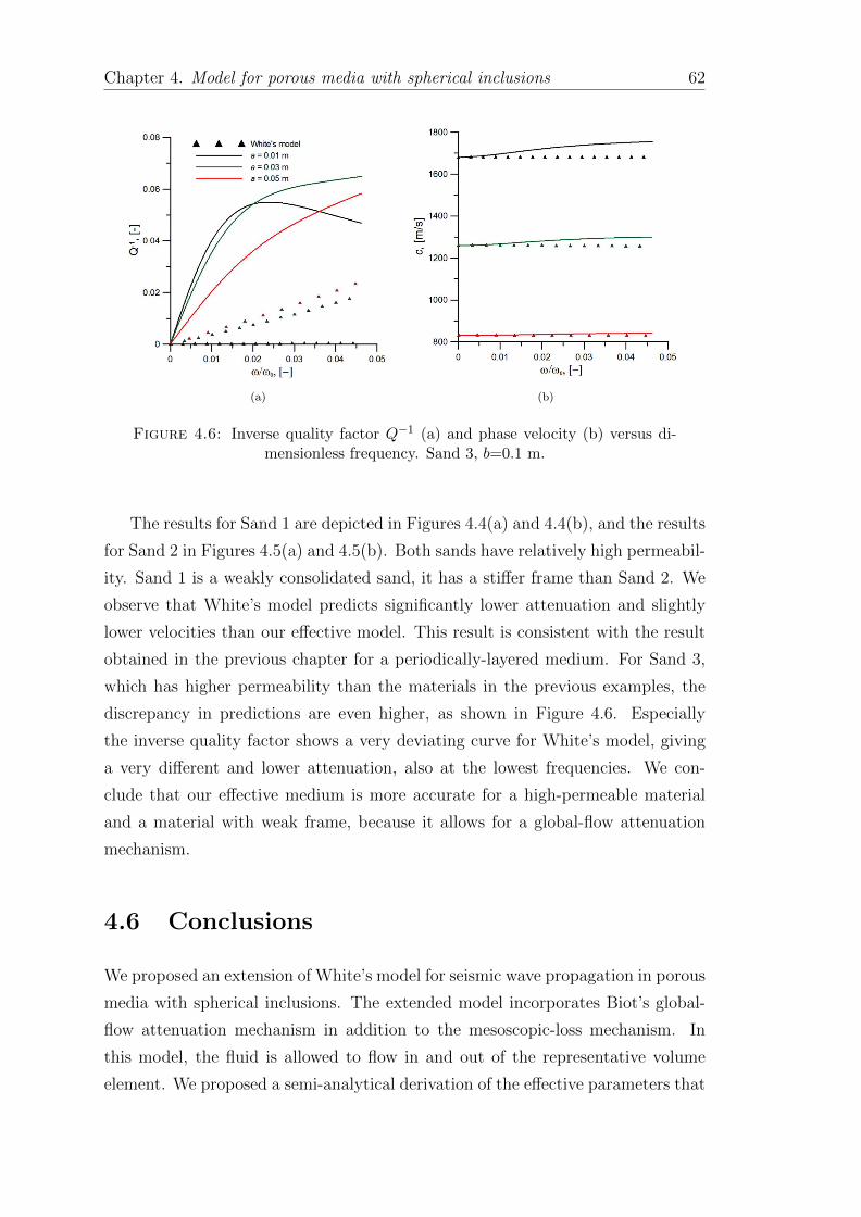
Chapter 4. Model for porous media with spherical inclusions 62
(a) (b)
Figure 4.6: Inverse quality factor Q−1 (a) and phase velocity (b) versus di-mensionless frequency. Sand 3, b=0.1 m.
The results for Sand 1 are depicted in Figures 4.4(a) and 4.4(b), and the results
for Sand 2 in Figures 4.5(a) and 4.5(b). Both sands have relatively high permeabil-
ity. Sand 1 is a weakly consolidated sand, it has a stiffer frame than Sand 2. We
observe that White’s model predicts significantly lower attenuation and slightly
lower velocities than our effective model. This result is consistent with the result
obtained in the previous chapter for a periodically-layered medium. For Sand 3,
which has higher permeability than the materials in the previous examples, the
discrepancy in predictions are even higher, as shown in Figure 4.6. Especially
the inverse quality factor shows a very deviating curve for White’s model, giving
a very different and lower attenuation, also at the lowest frequencies. We con-
clude that our effective medium is more accurate for a high-permeable material
and a material with weak frame, because it allows for a global-flow attenuation
mechanism.
4.6 Conclusions
We proposed an extension of White’s model for seismic wave propagation in porous
media with spherical inclusions. The extended model incorporates Biot’s global-
flow attenuation mechanism in addition to the mesoscopic-loss mechanism. In
this model, the fluid is allowed to flow in and out of the representative volume
element. We proposed a semi-analytical derivation of the effective parameters that

Chapter 4. Model for porous media with spherical inclusions 63
can be used as an input to Biot’s equations for homogeneous media. The predicted
attenuation and phase velocity are in good agreement with predictions by White’s
model when the global-flow mechanism is negligible. At higher frequencies, the
model predicts higher phase velocities than White’s model. For sandy sediments,
which are characterized by high permeability and a weak frame, White’s model
predicts significantly smaller attenuation. The result is in agreement with the
predictions obtained for periodically layered media (Chapter 3), where an exact
analytical solution is used for reference.
The proposed model can serve as a reference theoretical framework for predic-
tions of seismic attenuation in heterogeneous media, when the characteristic size
of heterogeneities is much smaller than the wavelength. It can also be used as a
benchmark solution for the models with a more complicated geometry, and to cali-
brate parameters in experimental studies. The model has wider applicability than
White’s model and other similar models where the no-flow boundary condition is
employed.
4.A Coefficients of system of linear equations for
cell problems
The systems of linear equations Ax = B(1,2) are solved to obtain the coefficients
αi in (4.15). Vectors B(1,2) contain the amplitudes of the applied total stress and
fluid pressure; they are defined in equations (4.11) and (4.12). Vector x contains
the unknown amplitudes:
x = [A1, C1, A2, B2, C2, D2] . (4.22)

Chapter 4. Model for porous media with spherical inclusions 64
The coefficients of the matrix A read
A11 = −j1(aII), A12 = −j1(cII), A13 = j1(aI)
A14 = j1(cI), A15 = y1(aI , A16 = y1(cI),
A21 = φIIP1A11, A22 = φIIP2A12, A23 = φIP1A13,
A24 = φIP2A14, A25 = φIP1A15, A26 = φIP2A16,
A31 = −λII1 j0(aII) + 2µII
((3a2II− 1)j0(aII + 3
aIIy0(aII)− 1
aIIj1(aII)
),
A32 = −λII2 j0(cII) + 2µII
((3c2II− 1)j0(cII + 3
cIIy0(cII)− 1
cIIj1(cII)
),
A33 = −(−λI1j0(aI) + 2µI
((3a2I− 1)j0(aI + 3
aIy0(aI)− 1
aIj1(aI)
)),
A34 = −(−λI1j0(cI) + 2µI
((3c2I− 1)j0(cI + 3
cIy0(cI)− 1
cIj1(cI)
)),
A35 = −(−λI1y0(aI) + 2µI
((3a2I− 1)y0(aI − 3
aIj0(aI)− 1
aIy1(aI)
)),
A36 = −(−λI1y0(cI) + 2µI
((3c2I− 1)y0(cI − 3
cIj0(cI)− 1
cIy1(cI)
)),
A41 = −(Q+βP1R
φ
)IIj0(aII), A42 = −
(Q+βP2R
φ
)IIj0(cII),
A44 = −(Q+βP2R
φ
)Ij0(cI), A45 = −
(Q+βP1R
φ
)Iy0(aI),
A43 = −(Q+βP1R
φ
)Ij0(aI), A46 = −
(Q+βP2R
φ
)Iy0(cI),
A51 = 0, A52 = 0, A53 = −(Q+βP1R
φ
)Ij0(bI), A54 = −
(Q+βP2R
φ
)Iy0(dI),
A55 = −(Q+βP1R
φ
)Iy0(bI), A56 = −
(Q+βP2R
φ
)Iy0(dI),
A61 = 0, A62 = 0,
A63 = −(−λI1j0(aI) + 2µI
((3b2I− 1)j0(bI + 3
bIy0(bI)− 1
bIj1(bI)
)),
A64 = −(−λI2j0(dI) + 2µI
((3d2I− 1)j0(dI + 3
dIy0(dI)− 1
dIj1(dI)
)),
A65 = −(−λI1y0(bI) + 2µI
((3b2I− 1)y0(bI − 3
bIj0(bI)− 1
bIy1(bI)
)),
A66 = −(−λI2y0(dI) + 2µI
((3d2I− 1)y0(dI − 3
dIj0(dI)− 1
dIy1(dI)
)),
(4.23)
where indices I and II correspond to the properties of the medium I (outer sphere)
and II (inner sphere), respectively. The symbols used in (4.23) are defined as
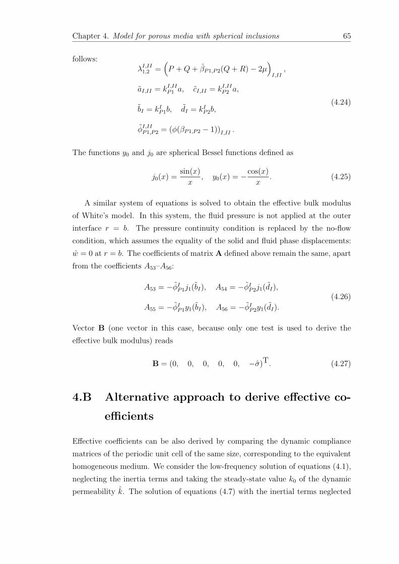
Chapter 4. Model for porous media with spherical inclusions 65
follows:λI,II1,2 =
(P +Q+ βP1,P2(Q+R)− 2µ
)I,II
,
aI,II = kI,IIP1 a, cI,II = kI,IIP2 a,
bI = kIP1b, dI = kIP2b,
φI,IIP1,P2 = (φ(βP1,P2 − 1))I,II .
(4.24)
The functions y0 and j0 are spherical Bessel functions defined as
j0(x) =sin(x)
x, y0(x) = −cos(x)
x. (4.25)
A similar system of equations is solved to obtain the effective bulk modulus
of White’s model. In this system, the fluid pressure is not applied at the outer
interface r = b. The pressure continuity condition is replaced by the no-flow
condition, which assumes the equality of the solid and fluid phase displacements:
w = 0 at r = b. The coefficients of matrix A defined above remain the same, apart
from the coefficients A53–A56:
A53 = −φIP1j1(bI), A54 = −φIP2j1(dI),
A55 = −φIP1y1(bI), A56 = −φIP2y1(dI).
(4.26)
Vector B (one vector in this case, because only one test is used to derive the
effective bulk modulus) reads
B = (0, 0, 0, 0, 0, −σ)T. (4.27)
4.B Alternative approach to derive effective co-
efficients
Effective coefficients can be also derived by comparing the dynamic compliance
matrices of the periodic unit cell of the same size, corresponding to the equivalent
homogeneous medium. We consider the low-frequency solution of equations (4.1),
neglecting the inertia terms and taking the steady-state value k0 of the dynamic
permeability k. The solution of equations (4.7) with the inertial terms neglected

Chapter 4. Model for porous media with spherical inclusions 66
can be found in the following form:
u = Ar +B
r2+ E2
(Cj1(qr) + Dy1(qr)
),
w = −E1
(Cj1(qr) + Dy1(qr)
),
(4.28)
where
q =
√iωη
k0
E1
E22 − E1E3
. (4.29)
The stress-strain relations (4.2) can be rewritten in terms of the displacements in
spherical coordinates:
τ = 3
(E1 −
4
3µ
)A− 4
µ
rE2
(Cj1(qr) + Dy1(qr)
),
p = −3E2A+ (E1E3 − E22)
(C
sin(qr)
r− Dcos(qr)
r
).
(4.30)
The unknown amplitudes Ai, Bi, Ci and Di, where i = 1, 2, correspond to the
solutions (4.28) of the inner sphere (blue area in Figure 4.2(a), i = 1) and the
outer sphere (grey area in Figure 4.2(a), i = 2). The displacement field should
be finite at r = 0, which means that B1 and D1 vanish. There are six unknown
amplitudes left. The cell problem is solved with the use of the same boundary
conditions, as discussed in Section 4.2.2. However, here both harmonic pressure
and total stress are applied at the outer interface of the cell in a single test.
The equations for the unknown amplitudes read Ax = B, where the structure of
matrix A is similar to matrix A, but the field variables are expressed with the use
of equations (4.28)–(4.30). Vector B reads
B = (0, 0, 0, 0, p, τ)T. (4.31)
The solution of the periodic-cell problem discussed above provides the frequency-
dependent elements of the dynamic compliance matrix (coefficients of proportion-
ality between the displacements and the applied stress τ and pressure p at r = b): u(b)
w(b)
=
α1 α2
α2 α3
τ
−p
. (4.32)
The elements of the compliance matrix αi in (4.32) depend on frequency and the
Chapter 4. Model for porous media with spherical inclusions 67
physical properties of the medium in the inner and outer spheres in the periodic
cell. In order to find the parameters of an equivalent homogeneous medium, we
compare the elements of the compliance matrix in (4.32) with the elements of
the compliance matrix obtained for a homogeneous periodic cell with the same
boundary conditions. For a homogeneous cell, the unknown amplitudes of the
displacement fields in (4.28) have to be found, in a similar way as for a non-
homogeneous cell. The amplitudes B and D in (4.28) vanish as u and w are finite
at r = 0, and the remaining amplitudes A and C are linear combinations of applied
stress τ and pressure p defined in the system of two linear algebraic equations, i.e.,
the continuity of total stress and fluid pressure (4.30) at r = b. The resulting
displacements at r = b read
u(b)
w(b)
=
bgqb∆
3bE1E2fqb∆
3bE1E2fqb∆
E1b(3E1 − 4µ)fqb∆
τ
−p
,where
gqb =(q2b2 sin(qb)
(E2
2 − E1E3
)− 3E2
2fqb),
fqb = sin(qb)− qb cos(qb),
∆ = sin(qb)q2b2(3E1 − 4µ)(E22 − E1E3) + 12E2
2µfqb.
(4.33)
The elements of the compliance matrix in (5.27) are frequency-dependent non-
linear transcendental functions of the medium parameters E1, E2, E3, η, µ, φ
and k0. We compare the zero-frequency approximation of the derived dynamic
compliance matrix in (5.27) with the matrix obtained in (4.32). The zero-frequency
approximation of (5.27) gives the following result: u(b)
w(b)
=
− bE3
∆bE2
∆
bE2
∆
b(4µ−3E1)
3∆
τ
−p
, (4.34)
in which ∆ = 3E22 − 3(E1 − 4µ)E3.
As in White’s model, we assume that the shear modulus remains the same
throughout the cell. Equating the compliance matrices in equations (4.32) and
(4.34) results in expressions for the frequency-dependent coefficients of the effective

Chapter 4. Model for porous media with spherical inclusions 68
homogenized medium:
E1 =1
3
α1b
α1α3 − α22
,
E2 = −1
3
α2b
α1α3 − α22
,
E3 =1
3
α3b
α1α3 − α22
+4
3µ.
(4.35)
The effective coefficients defined in (5.28) can be used to calculate the wavenum-
bers in the effective medium according to (5.29) and (5.30). The results obtained
with coefficients (5.28) coincide at low frequencies with the results obtained using
the coefficients (4.16).
Chapter 5
Higher-order elasticity models for
a periodically layered poroelastic
composite
In the previous chapters, effective models were derived with frequency-dependent
coefficients. The frequency dependence was introduced to account for attenuation
and dispersion caused by the presence of mesoscopic-scale heterogeneities. In this
chapter, alternative effective models for a periodically layered poroelastic medium
are proposed with coefficients that do not depend on frequency. This is advan-
tageous for calculations in the time domain, especially in multi-scale numerical
modelling.
5.1 Introduction
The effective homogenized models described in the previous chapters can be used
for modeling wave propagation in the domains where linear elasticity is assumed.
The frequency-dependent coefficients do not complicate the analysis as the linear
problems can be studied in the frequency-domain. However, time-domain analysis
is necessary to account for nonlinear effects that arise, for example close to a pow-
erful vibration source, or within a domain in which significant elastic deformations
or nonlinear fluid-solid interaction processes take place. As the time domain mod-
eling of large domains is computationally expensive, hybrid simulation approaches
are used, based on the application of the boundary element methods. The domain
where nonlinear deformations occur is linked to a domain where linear elasticity
69

Chapter 5. Higher-order continuum models 70
models apply using the time-domain Green’s functions. To enable efficient cou-
pling, the time-domain Green’s functions should be as simple as possible, which is
difficult to achieve when working with models that contain frequency-dependent
coefficients. This motivates introduction of a sufficiently accurate linear model
with coefficients that do not depend on frequency.
Higher-order continuum models are often used when more accurate descrip-
tion of the microstructure of a medium has to be taken into account, not captured
by the classical continuum. This is required, for example, to mimic dispersion
properties of an inhomogeneous medium for more accurate modeling. Higher-
order continuum models are used to account for the influence of the processes on
a microscale on a higher scale of observation (macroscale). Such models can be
derived by means of homogenization of continua with microstructure. They give
more accurate predictions compared to the classical continuum at shorter wave-
lengths. In this thesis, we are dealing with porous media containing mesoscopic
heterogeneities.
For the periodically layered porous media considered in Chapter 3, the mi-
crostructure is represented by the periodic cell, and a higher-order continuum can
be derived to account for the presence of layered heterogeneities. Higher-order ho-
mogenization was extensively studied for periodically layered elastic solids (Chen
and Fish, 2001, Fish et al., 2002, Andrianov et al., 2008). In this chapter, it is
applied to a poroelastic solid. Prior to that, we derive a higher-order viscoelas-
tic continuum from the dispersion equation obtained from White’s model (White
et al., 1975), by matching the associated dispersion relation and that of the pos-
tulated higher-order continuum model for low frequencies. The resulting equation
contains higher-order spatial and temporal derivatives of the displacement. Next,
homogenization with multiple spatial scales is applied to a poroelastic compos-
ite governed by Biot’s equations (Biot, 1956a). A method of asymptotic expan-
sions with multiple spatial scales (Benssousan et al., 1978, Sanchez-Palencia, 1980,
Bakhvalov and Panasenko, 1989) is extensively used for homogenization of hetero-
geneous media. In poroelasticity, the method was applied to derive macroscopic
equations of motion from microstructure by Burridge and Keller (1981). Similar
work was done by Levy (1979). Studies on higher-order homogenization of peri-
odic elastic composites can be found in Chen and Fish (2001), Fish et al. (2002)
and Andrianov et al. (2008). Further extensions to non-periodic cases and mul-
tiple dimensions are described in Capdeville et al. (2010a,b). The method and
its advantages are comprehensively described by Auriault (1980b, 2002), where

Chapter 5. Higher-order continuum models 71
examples are given, including porous-media examples. Homogenization with mul-
tiple scales is applied by Mei and Auriault (1989) to problems of flow in porous
media and consolidation. Here we apply the method to wave propagation in a
periodically layered poroelastic composite.
5.2 White’s model for periodically layered porous
media
The model of White et al. (1975) has been discussed in Chapter 3, where a solu-
tion in terms of the full Biot equations proposed by Dutta and Seriff (1979) and
Vogelaar and Smeulders (2007) was used in numerical examples. In this chapter,
we use the original solution by White et al. (1975), where an analytical expression
for the effective P-wave modulus K(ω) is given:
K(ω) =K∗
1 + i 2(RI−RII)2
ωL(ZI+ZII)
, (5.1)
where L is the length of a periodic cell, and other coefficients are defined in terms
of properties of the layers I and II:
1
K∗=
1− sKI
+s
KII
,
KI,II =
(Km +Ka
(1− Km
Ks
)2
+4
3µ
)I,II
,
RI,II =
((1− Km
Ks
)Ka
M
)I,II
,
ZI,II =
(Z0 cot
(1
2αwl
))I,II
,
(5.2)
where Km is a drained frame bulk modulus, µ is a shear modulus, Ks is the solid
grains bulk modulus, Kf is the bulk modulus of the pore fluid, φ is porosity, lI
and lII are the length of the layers I and II in the periodic cell, respectively, and

Chapter 5. Higher-order continuum models 72
s = lII/L. For each layer I and II
Ka =
(1− φKs
− Km
K2s
+φ
Kf
)−1
,
Z0 =√ηKei/(ωk0), αw =
√−iωη/(k0Ke),
Ke = Ka(Km +4
3µ)/K,
(5.3)
where η is the fluid viscosity and k0 denotes permeability of the solid frame.
The plane-wave modulus K(ω) defined in (5.1) is used in the description of one-
dimensional P-wave propagation in a viscoelastic medium governed by the follow-
ing equation of motion
− ω2ρu− K(ω)u,zz = 0, (5.4)
where the density term ρ = (1−s) (φρs + (1− φ)ρf )I+s (φρs + (1− φ)ρf )II and ρs
and ρf are the densities of the solid grains and fluid, respectively. The solution of
the equation (5.4) is u = A exp(−ikz), and the corresponding dispersion equation
reads
k2 = ω2 ρ
K(ω). (5.5)
5.3 Derivation of effective models with frequency-
independent coefficients
5.3.1 Viscoleastic model approximating White’s model dis-
persion relation
The equation of motion describing the effective medium is chosen such that it
predicts the same frequency dependence of the wavenumber as White’s model in
the frequency range of interest. The frequency dependence of k in (5.5) is rather
complicated. We expand ω2ρ/K(ω) in series of ω around ω = 0, up to the order
O(ω5):
k2 = f2ω2 − if3ω
3 − f4ω4 +O(ω5). (5.6)
Chapter 5. Higher-order continuum models 73
The expansion coefficients fi read:
f2 =ρ
H, H =
(K∗(RII −RI)
2 + Lg1
K∗Lg1
)−1
,
f3 =1
3iρ
(RII −RI)2g1g2
Lg21
,
f4 =1
45ρ
(RII −RI)2g3g2
Lg31
,
(5.7)
whereg1 = nIhII + nIIhI ,
g2 = n2In
2II ,
g3 = hIhII (n4I + 10g2 + n4
II) + 6nInII (n2Ih
2I + n2
IIh2II) ,
(5.8)
in which the following notations were introduced:
nI,II =
(η
Kek0
)I,II
, hI,II =
(ηKe
k0
)I,II
. (5.9)
Let us take the approximation k2 = f2ω2. This dispersion relation corresponds
to the classical wave equation, whose frequency domain form reads
− ρω2u−Hu,zz = 0. (5.10)
At the low frequency band, where f2 >> f3ω and f2 >> f4ω2, equation (5.6) can
be approximated by the following equations, in which ω2 in the terms proportional
to ω3 and ω4 is either fully or partially replaced by k2/f2:
k2 = f2ω2 − i
f3
f2
ωk2 − f4
f2
ω2k2, (5.11)
k2 = f2ω2 − i
f3
f2
ωk2 − f4ω4. (5.12)
Restricting the expansion order to ω3, the above equations can be further simplified
to
k2 = f2ω2 − i
f3
f2
ωk2. (5.13)

Chapter 5. Higher-order continuum models 74
The equations of motion, corresponding to equations (5.11)–(5.13) read
u,zz = f2u− f3f2u,zz + f4
f2u,zz,
u,zz = f2u− f3f2u,zz + f4
....u ,
u,zz = f2u− f3f2u,zz.
(5.14)
These are approximations of White’s model. They are also governed by the vis-
coelastic equations, as White’s model, but the effective coefficients do not depend
on frequency, and higher-order derivatives are introduced. We will now discuss
another approximation, where effective model is governed by the equations of
poroelasticity with higher-order terms. The results for all models are discussed in
Section 5.4.
5.3.2 Poroelastic model obtained from homogenization with
multiple spatial scales
Within the concept of separation of scales in the asymptotic two-scale homoge-
nization method of Sanchez-Palencia (1980), the macroscopic scale is associated
with some parameter of length L that is of the same order as the length of the trav-
elling wave, and the microscopic scale is the characteristic size of heterogeneities
which is the period of the system, the length of the unit cell L. The following
small parameter is introduced: ε = L/L. Two space variables are introduced:
x and y = x/ε. These variables are treated as two independent space variables
corresponding to the variations along the axis normal to the layering (denoted by
z in the previous section) on length scales L and L, respectively.
The displacement vector u = [u, w]T , where u and w are solid and relative
fluid-to-solid particle displacements, respectively, is looked for in the form of the
expansion
u = u0(x, y, t) + εu1(x, y, t) + ε2u2(x, y, t) + ..., (5.15)
where ui(x, y, t) are L-periodic with respect to y. Since y = y(x), the full spatial
derivative should now be expressed using the chain rule:
f;x = f,x + ε−1f,y, (5.16)

Chapter 5. Higher-order continuum models 75
where the semicolon in the subscript denotes the full derivative. The stress vector
σ = [τ,−p]T , where τ denotes the total stress τ = −σ−p, σ is intergranular stress
and p is pore fluid pressure. This vector is related to the displacement vector via
the stress-strain relations from Biot’s theory (Biot, 1956a):
σ = Eu;x, (5.17)
where matrix E is given below. Subsituting (5.15) into (5.17) and taking into
account (5.16) gives:
σ = ε−1σ−1(x, y, t) + σ0(x, y, t) + εσ1(x, y, t) + ε2σ2(x, y, t) + ..., (5.18)
whereσi = E (ui,x + ui+1,y) , i = 0, 1, 2, ...,
σ−1 = Eu0,y.
(5.19)
Each of the layers is governed by Biot’s equations of poroelasticity of (Biot,
1956a) reviewed in Chapter 2:
P(a,b)u(a,b) + B(a,b)u(a,b) − E(a,b)u;xx = 0, (5.20)
where superscripts a and b distinguish the regions 0 ≤ y ≤ sL and sL ≤ y ≤ L,
respectively. In equation (5.20) the elements of the matrices P, B and E contain
the physical properties of the layers corresponding to the regions a and b:
P =
(1− φ)ρs + φρf ρf
ρfαρfφ
,B =
0 0
0 b0φ2
,E =
P + 2Q+R Q+Rφ
Q+Rφ
Rφ2
.(5.21)
The following notations are used above: α is tortuosity and b0 is Biot’s viscous
factor b0 = ηφ2/k0. The poroelastic coefficients P , Q, R are given in (3.2).
The expansion of u (5.15) is substituted into the governing equation (5.20) for
each of the layers. Each power of ε in the resulting equation can be equated to
zero, thus forming a set of equations that is solved successively with the following
boundary conditions (i.e., L-periodicity of the displacement and stress vectors,

Chapter 5. Higher-order continuum models 76
and continuity of these vectors at the interface between the layers):
u(a)i (x, 0, t) = u
(b)i (x, L, t),
σ(a)i−1(x, 0, t) = σ
(b)i−1(x, L, t),
u(a)i (x, sL, t) = u
(b)i (x, sL, t),
σ(a)i−1(x, sL, t) = σ
(b)i−1(x, sL, t), i = 0, 1, 2, ... .
(5.22)
In addition, an averaging operator is introduced:
Ui(x, t) =1
L
sL∫0
u(a)i dy +
L∫sL
u(b)i dy
, i = 0, 1, 2, ... , (5.23)
where Ui(x, t) denotes the macroscopic displacement vector.
Equating the terms of ε−2 to zero, the following part from equation (5.20)
remains:
E(a,b)u(a,b)0,yy = 0. (5.24)
Solving this equation for the regions a and b using the boundary conditions (5.22)
(i = 0) leads to a simple result: u(a)0 = u
(b)0 = U0(x).
Equating the terms of ε−1 to zero gives
E(a,b)(u
(a,b)0,x + u
(a,b)1,y
),y
= 0. (5.25)
The solution of (5.25) is u(a)1 = a1y + b1 and u
(b)1 = c1y + d1, where a1, b1, c1
and d1 are the vectors of unknown functions of x and t found from the boundary
conditions (5.22) and related to U1 using (5.23).
Equating the terms of ε0 to zero results in the following equation:
P(a,b)u(a,b)0 + B(a,b)u
(a,b)0 − E(a,b)
(u
(a,b)0,xx + 2u
(a,b)1,xy + u
(a,b)2,yy
)= 0. (5.26)
Integrating (5.26) over the unit cell y = [0, L] and taking into account periodicity
of σ1 leads to the macroscopic equation of motion for U0:
P0U0 + B0U0 − E0U0,xx = 0, (5.27)

Chapter 5. Higher-order continuum models 77
where the matrices are defined as
P0 = sP1 + (1− s)P2, B0 = sB1 + (1− s)B2,
E0 = sE1 + (1− s)E2 + s(1− s)(E2 − E1)(sE2 + (1− s)E1)−1(E1 − E2).
(5.28)
For an elastic composite, the matrices in (5.28) reduce to scalars, and the matrix of
the effective moduli E0 reduces to the well-known harmonic average of the moduli
of the layers.
The next-order term u(a,b)2 is found by solving equation (5.26) in the form of
polynomial u(a,b)2 = a
(a,b)2 y2 + b
(a,b)2 y + c
(a,b)2 , where the vectors b
(a,b)2 and c
(a,b)2 are
found from the boundary conditions (5.22) and using the expression (5.23) for U2,
and the vectors a(a,b)2 are derived from equation (5.26).
Equating the terms of ε1 to zero gives:
P(a,b)u(a,b)1 + B(a,b)u
(a,b)1 − E(a,b)
(u
(a,b)1,xx + 2u
(a,b)2,xy + u
(a,b)3,yy
)= 0. (5.29)
Integrating (5.29) over the unit cell y = [0, L] and taking into account periodicity
of σ2 and the equation (5.27) leads to the macroscopic equation of motion for U1:
P0U1 + B0U1 − E0U1,xx = 0. (5.30)
The next-order term u(a,b)3 is found from the equation (5.29), similar to the previous
terms.
Equating the terms of ε2 to zero gives
P(a,b)u(a,b)2 + B(a,b)u
(a,b)2 − E(a,b)
(u
(a,b)2,xx + 2u
(a,b)3,xy + u
(a,b)4,yy
)= 0. (5.31)
Implementing the same integration as above, and taking into account (5.27) and
(5.30), we come to the macroscopic equation for U2:
P0U2 + B0U2 − E0U2,xx − L2(α1U0,xxxx + α2U0,xx + α3U0
)= 0. (5.32)
The expressions for the matrices α1−3 in this equation are given in Appendix 5.A.
In the absence of terms α2 and α3 (when there is no damping terms b0 in each of
the layers), (5.32) is canceled out to the equation obtained for the elastic composite
(Fish et al., 2002, Andrianov et al., 2008) assuming the matrices from (5.21) are
scalars.

Chapter 5. Higher-order continuum models 78
Now, we combine the macroscopic equations derived above to come up with a
single macroscopic description of the effective medium. The macroscopic displace-
ment, where orders up to ε2 are kept, reads: U = U0 + εU1 + ε2U2. Substitution
of U into the summation (5.27) + ε· (5.30) + ε2· (5.32) and keeping the terms up
to order ε0 results in
P0U + B0U− E0U,xx − L2(α1U,xxxx + α2U,xx + α3U
)= 0. (5.33)
Note that only one length scale L, which is the length of the periodic cell, is left
in the final equation (5.33). The length scale L is reduced in the multiplication
of ε = L/L to the last three terms in equation (5.32). The first three terms in
equation (5.33) are the classical Biot terms for a homogeneous medium with the
matrices of density and damping terms determined as the arithmetic averages of
the corresponding matrices of each of the layers, and the matrix of elastic moduli
determined as the harmonic average of the corresponding matrices of the layers.
As discussed above, a similar result is known for elastic composites, where the
effective density is the arithmetic average of the densities of the layers, and the
effective Young’s modulus is the harmonic average of the moduli of the layers. The
higher-order terms are corrections that explicitly contain information about the
scale of heterogeneities: apart from the properties of the layers and saturations,
they also depend on the characteristic size of heterogeneities, which is the length
of the periodic unit cell L.
The dispersion equation corresponding to equation (5.33) has four pairs of
roots with opposite signs. It predicts four P-waves in each direction: a fast and
a slow wave, as predicted by Biot’s theory, and two additional highly attenuated
waves, which are the results of the scattering of the fast and the slow wave by the
inhomogeneities. The corresponding wavenumbers are found as the roots of the
polynomial equation:
ω4(P1,1P2,2 − P1,2P2,1) + ω2(P1,2H2,1 − H1,1P2,2 + H1,2P2,1 − P1,1H2,2)k2+
(ω2L2(P1,1α2,21 − P1,2α
2,11 + P2,2α
1,11 − P2,1α
1,21 )− H2,1H1,2 + H1,1H2,2)k4+
L2(H1,2α2,11 + α1,2
1 H2,1 − H2,2α1,11 − H1,1α
2,21 )k6 + L2(α1,1
1 α2,21 − α
1,21 (α2,1
1 )k8 = 0,
(5.34)

Chapter 5. Higher-order continuum models 79
(a) (b)
Figure 5.1: Real (a) and imaginary (b) parts of the wavenumber predicted bydifferent models L=0.1 m, gas saturation 10%.
where αi,j1 are the elements of the matrix α1 and Pi,j and Hi,j are the elements of
the matricesP = P + B/(iω)− L2α3,
H = E0 + iωα2.
(5.35)
5.4 Results
In this section we compare predictions of dispersion and attenuation by the models
with frequency-independent coefficients discussed above. The material properties
of the solid frame in the example are those of Rock from Table 4.1. The pores are
fully saturated with water and gas (Table 3.2). It has been shown in Chapters 3
and 4 that White’s model is in agreement with the exact solution for this type of
material properties, therefore it is used here for reference.
In Figures 5.1–5.3, the real and imaginary parts of the wavenumbers are plotted
for different models: model 1 (equation 5.11), model 2 (equation 5.12), model 3
(equation 5.13), and model 4 (equation 5.34, the root corresponding to the fast
P-wave is considered). The results are plotted for a fixed periodic cell L = 0.1 m,
for saturations s = 10% (Figure 5.1), s = 50% (Figure 5.2) and s = 90% (Figure
5.3). As one can observe in all figures, the models obtained in the previous section
(model 4) predicts dispersion and attenuation only at low frequencies, and the
predictions deviate from the predictions of White’s model at higher frequencies.
For all models, the predictions are more accurate at high gas saturations. For

Chapter 5. Higher-order continuum models 80
(a) (b)
Figure 5.2: Real (a) and imaginary (b) parts of the wavenumber predicted bydifferent models L=0.1 m, gas saturation 50%.
(a) (b)
Figure 5.3: Real (a) and imaginary (b) parts of the wavenumber predicted bydifferent models L=0.1m, gas saturation 90%. On the rightmost panel all lines
for models 1–3 and White’s model coincide.
saturation s = 90% (Figure 5.3), all lines corresponding to models 1–3 coincide;
they are also very close to each other in Figure 5.2, for saturation s = 50%.
5.5 Conclusions
The method of asymptotic expansions with multiple spatial scales was applied
to wave propagation in a poroelastic composite with a periodically repeated unit
cell that consists of two layers with different properties, each layer governed by

Chapter 5. Higher-order continuum models 81
Biot’s equations. The results show that this model underestimates attenuation;
its performance is getting worse at higher frequencies. One should note that the
method of asymptotic expansions is formally only correct when the physical con-
stants are of the same order, which is not always the case for poroelastic constants
in media with heterogeneities, especially when heterogeneities occur in saturating
fluid properties. That is why models obtained directly from White’s model pro-
vide more accurate predictions of attenuation. These models are also viscoelastic
models, like the model of White, but incorporate higher-order derivatives to ac-
count for the presence of heterogeneities. They can be used at sufficiently low
frequencies for thinly layered poroelastic composites, where the model of White is
also applicable. The advantages of models with coefficients that do not depend on
frequency is the possibility to use them for efficient time-domain computations.
5.A Effective coefficients
The expressions for the matrices α1, α2 and α3 from equation (5.33) are given in
this appendix. The expression for α1 reads
α1 = −c1
(P−1
0 E0
)2+ c2P
−10 E0 + c3, (5.36)
where
c1 = 112
(P1 −P2)(s(s3 − s2)E−1
1 P1 + s(−s3 + 3s2 − 3s+ 1)E−12 P2
), (5.37)

Chapter 5. Higher-order continuum models 82
c2 = s(P1−P2)12
((2s2 − 4s+ 2)D(E1 − E2) + (2s2 − 3s+ 1)I) +
E1−E2
12s2[((9s3 − 3s5 − 6s2)DE1 + (s6 − 9s5 + 2s4 + 6s3)I)DP1 −D((2s4 − s5 − s3)P1
−(6s4 − 6s3)P2)D(E1 − E2)− (s6 − s5)(DE2 − I)E−11 P1
−D((3s5 − 12s3 + 6s2 + 9s− 6)E1 − 3s(s− 1)(s3 + 3s2 − s− 3)E2)DE1E−12 P2
+DE2D((18s3 − 6s5 − 12s4)P2 + 3s2(s3 + 2s2 − 3s)P1)+
((s6 + 11s5 + 3s4 − 7s3 − 8s2)I + 6s2(s3 − 3s+ 2)DE1)DP2+
((13s2 − s5 − 3s4 − 5s3 + 6s− 10)sDE1 + s2(s− s4 − s3 − 3s2 + 4)I)E−12 P2
+(s(6s2 − s4 − 2s3 − 2s− 1)DE1 + s2(3s− s3 − 3s2 + 1)I)E−12 P2D(E1 − E2)
],
(5.38)
c3 = E1−E2
12s[((2s4 + 3s3 − s2 − 4s)I + D (E1(19s4 + 10s3 − 24s2 − 15s+ 10)+
E2(12s2 − 19s4 − 10s3 + 17s) + DE1D(2s(13s5 − s4 − 28s3 + 4s2 + 15s− 3)E1+
(2s3 − 26s4 + 53s2 − 8s− 21)E2) + DE2D((26s4 + 28s3 − 32s2 − 22s)E2+
(35s2 − 26s4 − 28s3 + 28s− 9)E1) + 3D((1s(3s5 − s4 − 11s3 + 9s2 + 4s− 4)E1
−(3s4 + 5s3 − 13s2 − s+ 6)E2)DE1 + ((s(3s3 + 7s2 − 7s− 3)E2−
− (s− 1)(3s3 + 4s2 − 5s− 2)E1)DE2) D(E1 − E2)] .
(5.39)
In equations (5.37)–(5.39),
D = s(sE2 + (1− s)E1)−1, I is an identity matrix. (5.40)
The expression for α2 is
α2 = c1
(P−1
0 E0P−10 B0 + P−1
0 B0P−10 E0
)− c2P
−10 B0 + c4 − c5P
−10 E0, (5.41)

Chapter 5. Higher-order continuum models 83
where
c4 = s(B1−B2)12
((2s2 − 4s+ 2)D(E1 − E2) + (2s2 − 3s+ 1)I) +
E1−E2
12
[(s+ 4− s4 − s3 − 3s2)I + 1
s(13s2 + 6s− 10− s5 − 3s4 − 5s3)DE1
+(s4 + 11s3 + 3s2 − 7s− 8)DE2 − 3s2
(s5 − 4s3 + 2s2 + 3s− 2)DE1DE1+
+(6s3 − 18s+ 12)DE1DE2 + 3s(s− 1)(s3 + 3s2 − s− 3)DE2DE1−
−6s(s2 + 2s− 3)DE2DE2)E−12 B2 + ((3s+ 1− s3 − 3s2)I+
+6s(s− 1)DE2 + 1s(6s2 − 2s− 1− s4 − 2s3)DE1)E−1
2 B2D(E1 − E2)+
+((s4 − s3)I + s(s3 − 9s2 + 2s+ 6)DE1 + (9s− 3s3 − 6)DE1DE1+
+(s3 − s4)DE2 + (3s3 + 6s2 − 9s)DE2DE1)E−11 B1+
+ s(s2 − 2s+ 1)DE1E−11 B1D(E1 − E2)
].
c5 = 112
(P1 −P2) s((s3 − s2)E−11 B1 + (3s2 − s3 − 3s+ 1)E−1
2 B2)+
+ 112
(B1 −B2) s((s3 − s2)E−11 P1 + (3s2 − s3 − 3s+ 1)E−1
2 P2).
(5.42)
The expression for α3 is
α3 = −c6 + c5B−10 E0 − c1(P−1
0 B0)2, (5.43)
where
c6 =1
12(B1 −B2) s((s3 − s2)E−1
1 B1 + (3s2 − s3 − 3s+ 1)E−12 B2). (5.44)

Chapter 6
An effective anisotropic
poroelastic model for elastic wave
propagation in finely layered
media
In this chapter, a new effective poroelastic model for finely layered media is pre-
sented and its performance is evaluated focusing on the angle-dependent atten-
uation behavior. To enable this, an exact solution is obtained for the response
of a periodically layered medium to a surface point load using Floquet’s theory.
This solution is compared to that of the new model and the equivalent viscoelastic
VTI medium available from existing literature. It is observed that the qP-wave
dispersion and attenuation is predicted with high accuracy by the new effective
poroelastic model. For the qS-wave, the effective poroelastic model provides a
perceptibly better prediction of the attenuation, resulting in closer to the exact
waveforms. The qS-wave attenuation is underestimated by the effective viscoelas-
tic model, while for the qP-wave the model gives accurate predictions in all cases
except for highly permeable weak-frame media.
This chapter was submitted for publication as a journal paper to Geophysics. Note thatminor changes have been introduced to make the text consistent with the other chapters of thisthesis.
85

Chapter 6. 2-D poroelastic model for layered media 86
6.1 Introduction
Horizontally layered models are commonly used for the analysis of wave propaga-
tion in reservoir rocks and sediments. This is a compromise between a relatively
accurate representation of heterogeneities in rocks and simplicity of computations.
Assuming lateral homogeneity of a reservoir is reasonable because the variations
in rock properties in the direction normal to the layering are typical for most
reservoir rocks and sediments. Layered models allow to study the effects of local
inhomogeneities at the macroscopic scale. The layers can represent mesoscopic-
scale heterogeneities when their thicknesses are much larger than the typical pore
and grain sizes, but smaller than the wavelength of a propagating wave. Meso-
scopic heterogeneities are known to cause strong dispersion and attenuation of
seismic waves due to the sub-wavelength scale wave-induced fluid flow (Muller
et al., 2010). The attenuation is particularly strong when a medium is saturated
with different fluids with a large contrast in compressibility (White et al., 1975,
Carcione and Picotti, 2006).
The commonly used equations for description of wave propagation in fluid-
saturated media are Biot’s equations of poroelasticity (Biot, 1962). This theory
predicts one shear and two compressional waves in a macroscopically homoge-
neous medium. It is widely accepted that Biot’s theory underestimates observed
attenuation and dispersion of elastic waves (Johnston et al., 1979; Winkler, 1985;
Gist, 1994). One of the reasons is a violation of the assumption of uniform sat-
uration with a single fluid. Inhomogeneities in solid-frame properties also cause
attenuation. Many models for wave propagation in heterogeneous porous media
were developed to address this effect. Each model proposes an attenuation mech-
anism which is based on certain assumptions. These assumptions are related,
among other things, to the scale of the heterogeneities and their distributions, and
the frequency range of interest. Depending on the scale of observations, different
models are used to study wave attenuation and dispersion. Attenuation due to
dissipation at the pore scale is described by a squirt-flow mechanism (O’Connell
and Budiansky, 1977; Mavko and Nur, 1979; Palmer and Traviola, 1980; Dvorkin
and Nur, 1993). Differences in fluid saturation between thin compliant pores and
larger stiffer ones, the presence of thin cracks, different shape and orientation of
the pores, as well as distribution of immiscible fluids in a pore cause attenuation
and dispersion due to local or squirt flow. This mechanism usually plays a role
at ultrasonic frequencies. At seismic frequencies another attenuation mechanism
Chapter 6. 2-D poroelastic model for layered media 87
caused by the subwavelength-scale fluid flow due to the presence of mesoscopic-
scale heterogeneities plays a role. This mechanism is not captured by Biot’s theory
which accounts for a global (wavelength-scale) flow attenuation mechanism. Since
gas, oil and water are often present in rocks and sediments as mesoscopic-scale
patches, multiple models are being developed that describe attenuation of seismic
waves in such heterogeneous media.
One of the pioneering works on seismic attenuation caused by the wave-induced
fluid flow is the work of White et al. (1975), in which a periodically layered
porous medium was considered and a frequency-dependent plane-wave modulus
was derived for normal wave incidence. Similar but differently derived moduli
were reported in other publications: e.g., Norris (1993), Brajanovski and Gure-
vich (2005) and Vogelaar and Smeulders (2007). Some other models of effective
P-wave moduli make use of a frequency-dependent branching function that con-
nects the low- and high-frequency limits (e.g., Johnson, 2001). This approach was
used by Krzikalla and Muller (2011), who introduced an effective vertical trans-
verse isotropic (VTI) medium to describe propagation of qP- and qS-waves at
different angles. In their model, the low- and high-frequency elastic moduli from
poroelastic Backus averaging by Gelinsky and Shapiro (1997) are connected by
a frequency-dependent function — the effective P-wave modulus of White et al.
(1975) for periodic layering and normal incidence. For a randomly layered medium
with a small fluctuation of parameters, the frequency-dependent function can be
derived from Gelinsky et al. (1998). With the approach used by Krzikalla and
Muller (2011), any model where a plane-wave modulus for P-wave propagation
normal to the layering is derived can be extended for arbitrary angle of incidence.
Another approach to compute the frequency-dependent coefficients of the effective
VTI medium numerically was proposed by Carcione et al. (2011). The resulting
effective medium in both approaches is governed by the equations of a viscoelastic
VTI medium and has five complex-valued frequency-dependent stiffnesses. This
means that the fluid-to-solid relative motion is not explicitly present in the model.
Instead, the information about attenuation caused by the interaction of the fluid
and solid phases at the subwavelength-scale is included in the frequency depen-
dence of the effective stiffnesses. Furthermore, this effective model does not predict
a slow P-wave on a macroscopic scale, as predicted by Biot’s theory. On the one
hand, this is advantageous from the computational point of view as the presence of
the slow wave requires a very fine meshing in 3-D numerical simulations. On the
other hand, the Biot’s global flow mechanism — macroscopic attenuation due to

Chapter 6. 2-D poroelastic model for layered media 88
viscous forces between fluid and solid phases — is not captured in the equations of
viscoelasticity, which may be disadvantageous even in the seismic frequency range
(Kudarova et al., 2013, this thesis, Chapter 3).
In this chapter, we combine the effective constants from the poroelastic Backus
averaging (Gelinsky and Shapiro, 1997) and the method proposed by Krzikalla
and Muller (2011). We use the effective P-wave moduli introduced in Chapter
3. This results in the effective stiffnesses of an effective poroelastic VTI medium
governed by Biot’s equations. This effective medium accounts for the macroscopic
(Biot’s global-flow) attenuation via the effective inertia and viscous terms used in
Biot’s equations, and for the mesoscopic (sub-wavelength scale) attenuation via the
frequency-dependence of the effective stiffnesses. We consider wave propagation in
a 2-D half-space, subject to a point-source at the surface. Solutions to this problem
are obtained for the effective viscoelastic model mentioned above and for the newly
derived poroelastic model. As a reference, an exact analytical solution is obtained
with the use of Floquet’s theory (Floquet, 1883). The responses predicted by all
three solutions are compared.
The chapter is structured as follows. First, Biot’s equations are briefly re-
viewed, and the exact analytical solution for a periodically layered medium is
formulated using Floquet’s theory. Secondly, the equations for the effective vis-
coelastic model are presented. Then, the effective poroelastic model is introduced.
The numerical examples follow, and the discussion of the results and conclusions
finalize the chapter.
6.2 Theoretical models
In this section, we present the equations of Biot’s theory, followed by the equations
of the effective viscoelastic model and the derivation of the effective poroelastic
model. The exact solution for a periodically layered medium governed by Biot’s
equations is given in Appendix 6.A.

Chapter 6. 2-D poroelastic model for layered media 89
6.2.1 Biot’s theory
Biot’s equations of motion read (Biot, 1962)
τij,j = ρui + ρf wi,
−p,i = ρf ui +αijρfφ
wj + ηrijwj.(6.1)
Throughout this chapter, comma in the subscript denotes a spatial derivative, an
overdot denotes a time derivative, and repeated indices are summed over. The fol-
lowing notations are used: ρf , ρs are fluid and solid grain densities, respectively;
φ is porosity, and the total density ρ = (1 − φ)ρs + φρf ; αij = α∞δij, where α∞
is the tortuosity, δij is the Kronecker delta, and η is the fluid viscosity; τij are the
elements of the total stress tensor, p is the fluid pressure, and u and w are the dis-
placements of the solid phase and the relative fluid-to-solid displacement multiplied
by φ, respectively. Tensor r = k−10 , where the elements of k0 are the permeabil-
ities kij, and for the isotropic case kij = k0δij. The high-frequency correction to
Biot’s viscous damping factor is commonly adopted to account for dynamic effects,
resulting in the dynamic permeability k0 = k0(√
1 + iωM/(2ωB) + iω/ωB)−1 [and
consequently, temporal convolution in (6.1)], where M is the parameter that de-
pends on the pore geometry, permeability and porosity; throughout the chapter,
we assume M = 1 (Johnson et al., 1987). The real part of the square root is
taken greater than zero. Biot’s critical frequency ωB = φη/(k0α∞ρf ) separates
the regimes where inertial and viscous forces dominate.
Throughout the chapter, a hat above a quantity stands for frequency depen-
dence and a tilde stands for frequency-wavenumber dependence. The Fourier
transform is applied for transforming to the frequency-wavenumber domain:
f(kx, z, ω) =
∞∫−∞
∞∫−∞
exp(−iωt) exp(ikxx)f(x, z, t)dtdx. (6.2)
The inverse Fourier transform is formulated in a following way:
f(x, z, t) =1
2π2
∞∫0
Re
∞∫−∞
f(kx, z, ω) exp(iωt) exp(−ikxx)dkx
dω. (6.3)
Only positive frequencies are considered, as the negative frequency components do
not provide information independent of the positive components (Wapenaar and

Chapter 6. 2-D poroelastic model for layered media 90
Berkhout, 1989). We study propagation of the plane waves in the x − z plane,
where x is the horizontal direction, and z is the vertical direction.
The stress-strain relations for an isotropic medium read
τxx = E1ux,x + (E1 − 2µ)uz,z + E2(wx,x + wz,z),
τzz = (E1 − 2µ)ux,x + E1uz,z + E2(wx,x + wz,z),
τxz = µ(ux,z + uz,x),
−p = E2(ux,x + uz,z) + E3(wx,x + wz,z),
(6.4)
where the coefficients are defined as follows (Biot, 1962):
E1 = P + 2Q+R, E2 = (Q+R)/φ, E3 = R/φ2,
P =φKm + (1− φ)Kf (1− φ−Km/Ks)
φ+Kf (1− φ−Km/Ks) /Ks
+4
3µ,
Q =φKf (1− φ−Km/Ks)
φ+Kf (1− φ−Km/Ks) /Ks
,
R =φ2Kf
φ+Kf (1− φ−Km/Ks) /Ks
.
(6.5)
In the above equations, Ks, Kf and Km are the bulk moduli of the solid grains,
fluid and the drained frame, respectively; µ is the shear modulus of the drained
frame.
In the frequency-wavenumber domain, we look for plane-wave solutions of the
equations (6.1) in the form
u = (Ux, Uz, Wx, Wz)T exp(−ikzz). (6.6)
In the isotropic case, the P- and S-wave motions are decoupled. The corresponding
dispersion relations are obtained by introducing the displacement potentials [φs,
ψs, φf , ψf ] = [Φs, Ψs, Φf , Ψf ] exp(−ikzz), where
ux = −ikxφs − ψs,z, wx = −ikxφf − ψf,z,
uz = φs,z − ikxψs, wz = φf,z − ikxψf .
(6.7)

Chapter 6. 2-D poroelastic model for layered media 91
Substitution of these relations into (6.1) leads to the dispersion equation
{(E1E3 − E2
2)s4 − (ρE3 + mE1 − 2ρfE2)s2 + ρm− ρ2f
}{µms2 − ρm+ ρ2
f
}= 0.
(6.8)
In equation (6.8), s =√k2x + k2
z/ω denotes slowness. The operator m = ρfα∞/φ+
b/(iωφ2), where b = b0
√1 + iω/(2ωB) is the dynamic viscous factor (the real part
of the square root is positive), and b0 = ηφ2/k0. The first term between curly
brackets in (6.8) is a dispersion equation for P-waves and the second one for S-
waves.
6.2.2 Effective viscoelastic VTI model
We first introduce the equations for the effective viscoelastic model, and then the
additional parameters are defined to obtain the equations of motion for the effective
poroelastic model, given in the next section. The effective vertical transversely
isotropic (VTI) model for wave propagation in layered media at arbitrary angle
was presented by Krzikalla and Muller (2011). This effective model makes use of
the poroelastic Backus averaging (Gelinsky and Shapiro, 1997) and the effective
plane-wave modulus obtained for a periodic 1-D medium (White et al., 1975).
The resulting equations in the effective medium are equations of elasticity with
frequency-dependent coefficients. Throughout the chapter, we refer to this model
as the viscoelastic model.
The analysis of dispersion and attenuation predicted by this model for media
with inhomogeneities in frame properties was carried out by Krzikalla and Muller
(2011). In the current chapter, we present the space-time domain responses of
the effective medium to a surface point load. We discuss examples with inho-
mogeneities both in solid frame and fluid properties. The equations used in this
analysis are outlined below.
The equations of motion for the effective VTI viscoelastic model read
−ikxτxx + τxz,z = −ω2ρux,
−ikxτxz + τzz,z = −ω2ρuz,
(6.9)
where ρ is the density of the homogenized medium obtained by averaging over
the layers 1 and 2 of the periodic cell: ρ = 〈ρ(z)〉. Throughout the chapter, the

Chapter 6. 2-D poroelastic model for layered media 92
angular brackets denote averaging over the layers in the periodic cell
〈f〉 =1
L
∫L
f(z)dz. (6.10)
The stress-strain relations for the effective viscoelastic VTI model read
τxx = −ikxAux + F uz,z,
τxz = D(ux,z − ikxuz),
τzz = −ikxF ux + Cuz,z.
(6.11)
In the effective medium, the stiffnesses in the above equations are frequency de-
pendent. The expressions for the effective stiffnesses A, F , C and D were obtained
by Gelinsky and Shapiro (1997) in two limiting cases of relaxed and unrelaxed pore
pressures (the expressions are given in Appendix 6.C). These limits are referred
to as quasi-static and no-flow limits, respectively. It is assumed that the fluid flow
is independent of the loading direction (i.e., direction of wave propagation), and
a single relaxation function connects the relaxed and unrelaxed limits of the effec-
tive stiffnesses. This function is based on a frequency-dependent modulus K(ω),
derived originally by White et al. (1975). The expression for K(ω) is given in
Appendix 6.C. The normalized relaxation function reads
R(ω) =K(ω)− Cu
Cr − Cu, (6.12)
where the superscripts r and u refer to the relaxed and unrelaxed limits, respec-
tively. The effective stiffnesses then read{A, C, F , D
}= {A,C, F,D}u − R(ω)({A,C, F,D}u − {A,C, F,D}r). (6.13)
It follows from (6.13) that C = K(ω). Since the shear modulus does not depend
on the fluid pressure, it is the same in the relaxed and the unrelaxed cases, and
the effective shear modulus D does not depend on frequency:
D = D = Du = Dr =
⟨1
µ
⟩−1
. (6.14)

Chapter 6. 2-D poroelastic model for layered media 93
To obtain the dispersion equations of the effective viscoelastic VTI model, we look
for the solution of (6.9) in the frequency-wavenumber domain in the form
(ux, uz) = (Ux, Uz) exp(ikzz). (6.15)
Substituting this into the equation of motion (6.9) and taking into account (6.11),
provides the following solutions of the dispersion equation:
k±1z = ±
√ε1 +
√ε2
2DC, k±2z = ±
√ε1 −
√ε2
2DC,
ε1 = ρ(C +D)− (AC − 2DF − F 2)k2x,
ε2 = (A2C2 − 4(AC + F )D − 2F 2(AC − 2D2) + F 3(4D + F ))k4x+
+2ρ(F (D + C)(F + 2D) + CD(2D + A)− AC2)k2x + ρ2(C −D)2.
(6.16)
The pairs of the wavenumbers k±1z,2z correspond to up- and downgoing quasi-P
(qP) and quasi-S (qS) waves. The amplitude ratios Uz/Ux read:(Uz
Ux
)±1,2
=ρω2 − Ak2
x −D(k±1z,2z
)2
(F +D)kxk±1z,2z
. (6.17)
6.2.3 Effective poroelastic VTI model
In this section, we introduce the effective poroelastic model based on the poroe-
lastic Backus averaging (Gelinsky and Shapiro, 1997) and the effective plane-wave
moduli obtained for P-wave propagation at normal incidence in a periodically
layered porous medium (Kudarova et al., 2013; this thesis, Chapter 3). These ef-
fective moduli result from employing the boundary conditions at the interfaces of
the periodic cell, different from those used in White’s model (White et al., 1975).
The no-flow condition is replaced with the pressure continuity condition, allowing
fluid flow at the macroscopic scale. As a result, two additional plane-wave moduli
are derived to describe the effective medium with Biot’s equations. These effec-
tive moduli are used to define the effective stiffnesses B6, B7, B8 (notation used
as in Gelinsky and Shapiro, 1997) required to describe the effective poroelastic
VTI model. Apart from the effective stiffnesses, the effective densities have to
be defined. We use the results obtained by Molotkov and Bakulin (1999), who

Chapter 6. 2-D poroelastic model for layered media 94
showed that the effective medium representing a stack of Biot layers is a general-
ized transversely isotropic Biot medium. In this poroelastic medium, the densities
and the viscous terms in Biot’s equations are defined differently in the x and z
directions. The equations of motion read
−ikxτxx + τxz,z = −ω2ρxux − ω2ρfxwx,
−ikxτxz + τzz,z = −ω2ρzuz − ω2ρfzwz,
ikxp = −ω2ρfxux − ω2mxwx,
−p,z = −ω2ρfzuz − ω2mzwz,
(6.18)
where the coefficients on the right-hand side read (Molotkov and Bakulin, 1999):
ρfx =s1ρf1m2 + s2ρf2m1
s1m2 + s2m1
, mx =
⟨1
m
⟩−1
,
ρx = 〈ρ〉 − s1s2(ρf1 − ρf2)2
s1m2 + s2m1
,
ρz = 〈ρ〉 , ρfz = 〈ρf〉 , mz = 〈m〉 .
(6.19)
The indices 1 and 2 in equations (6.19) refer to the layers 1 and 2. The volume
fractions of the layers are s1 = l1/L, s2 = l2/L.
The stress-strain relations read
τxx = −ikxAux + F uz,z + B6(−ikxwx + wz,z),
τzz = −ikxF ux + Cuz,z + B7(−ikxwx + wz,z),
τxz = D(ux,z − ikxuz),
−p = −ikxB6ux + B7uz,z + B8(−ikxwx + wz,z).
(6.20)
The frequency-dependent stiffnesses in (6.20) are defined in the same way as in
the effective viscoelastic model, but the frequency dependence is incorporated via
the effective plane-wave moduli obtained with the method proposed by Kudarova
et al., 2013 (this thesis, Chapter 3).
These effective moduli are obtained from the solution of the 1-D problem for
the periodic cell consisting of two isotropic layers (see Figure 3.1) where harmonic
stress and pressure are applied to the outer edges of the cell normal to the layering.
Chapter 6. 2-D poroelastic model for layered media 95
The layers are governed by Biot’s equations (6.1) (with z-dependent field variables
uz, wz, τzz and p). The problem is solved in the frequency domain. In each layer
the displacements uz and wz are found as up- and down-going plane waves (a fast
and a slow P-wave), resulting in eight unknown amplitudes. These amplitudes
are found from the following boundary conditions: continuity of the intergranular
stress σzz, pore pressure p, displacements uz and wz at the interface between the
layers, and continuity of the total stress τzz and pressure p at the outer edges
of the cell. The strains uz,z and wz,z are found as the difference between the
displacements at the outer edges of the unit cell, divided by the cell width. This
gives us the coefficients of the frequency-dependent symmetric compliance matrix
αij:
uz,z = α11τzz + α12p,
wz,z = α12τzz + α22p.
(6.21)
They are equated to the coefficients of the compliance matrix obtained from Biot’s
stress-strain relations (6.4) (for the 1-D case, with kx = 0):
uz,z = 1
∆
(E3τzz + E2p
),
wz,z = 1
∆
(−E2τzz − E1p
), ∆ = E1E3 − E2
2 .
(6.22)
Then, the frequency-dependent elastic parameters E1, E2, E3 are found, describ-
ing attenuation and dispersion due to wave-induced mesoscopic fluid flow in 1-D
periodically layered medium:
E1 =α22
α11α22 − α212
, E2 = − α12
α11α22 − α212
, E3 =α11
α11α22 − α212
. (6.23)
The coefficients αij are computed numerically by solving a system of eight by eight
linear algebraic equations corresponding to eight boundary conditions in the cell
problem (for more details, see Chapter 3).
Following Krzikalla and Muller (2011), we introduce a branching function
R1(ω) =E1(ω)− Cu
Cr − Cu. (6.24)
to obtain the frequency-dependent effective moduli A, C and F :{A, C, F
}= {A,C, F}u − R1(ω)({A,C, F}u − {A,C, F}r). (6.25)

Chapter 6. 2-D poroelastic model for layered media 96
As discussed above, the modulus D is not frequency dependent, and is defined in
equation (6.14). Note that R1(ω) is equivalent to R(ω) (equation (6.12)) when
the frequency is much lower than Biot’s critical frequency ωB. The effective plane-
wave modulus E1 is an extension of White’s frequency-dependent modulus K(ω)
to higher frequencies, first proposed by Vogelaar and Smeulders (2007). Further
generalization was proposed by Kudarova et al., 2013 (this thesis, Chapter 3),
where the no-flow boundary conditions at the outer edges of the unit cell were
replaced by the pressure continuity condition, allowing the global flow to take
place. This results in additional effective moduli E2 and E3 used to describe the
effective Biot medium.
By comparing the expressions for τzz and p in equations (6.4) (with incor-
porated frequency-dependent coefficients E1, E2 and E3 introduced above) and
(6.20), we can find out how the other moduli of the effective poroelastic VTI
model should be chosen. First, it can be observed that
B7 = E2, B8 = E3. (6.26)
Next, the effective coefficient B6 should be obtained. In the particular case when
the shear modulus is constant throughout the layers, there is no anisotropy in
the stiffness matrix of the effective poroelastic medium, and B6 = B7 = E2.
Anisotropy remains in the viscous and inertia terms, according to their definition
in (6.19). In the general case, complying with the method used by Krzikalla
and Muller (2011), the frequency-dependence of B6 is specified using a second
normalized relaxation function:
R2(ω) =E2 −Bu
7
Br7 −Bu
7
. (6.27)
The final expression for the effective modulus B6 then reads
B6 = Bu6 − R2(ω)(Bu
6 −Br6). (6.28)
Now, all effective constants have been determined. For clarity, we underline
that the effective poroelastic model incorporates both the mesoscopic and the
macroscopic attenuation mechanisms; the former is captured by the effective stiff-
nesses in equation (6.20), while the latter comes in through the effective terms
defined in equation (6.19).
Chapter 6. 2-D poroelastic model for layered media 97
To obtain the dispersion equation of the effective poroelastic VTI model, we
look for the solution of equations (6.20) in the form
{ux, uz, wx, wz} ={Ux, Uz, Wx, Wz
}exp(−ikzz). (6.29)
Substitution of (6.29) into stress-strain relations (6.20) and the equations of motion
(6.18) gives the dispersion relation det(M) = 0 with solutions kz(kx, ω), where M
is a matrix with coefficients given as:
M =
Ak2x +Dk2
z − ω2ρx (D + F )kxkz B6k2x − ω2ρfx B6kxkz
(F +D)kxkz Ck2z +Dk2
x − ω2ρz B7kxkz B7k2z − ω2ρfz
−B6k2x + ω2ρfx −B7kxkz −B8k
2x + mxω
2 −B8kxkz
−B6kxkz −B7k2z + ω2ρfz −B8kxkz −B8k
2z + mzω
2
.
(6.30)
The equation det(M) = 0 provides the dispersion relation:
c1k6z + c2k
4z + c3k
2z + c4 = 0. (6.31)
Explicit expressions for the coefficients ci are not presented here for the sake of
brevity; they can be expressed in terms of the elements of the matrix M. The
solution of (6.31) is
k±1z = ±√
a6c1− 2
3
3c1c3−c22c1a
− c23c1,
k±2z = ±√−(1− i
√3) a
12c1+ 2(1 + i
√3)
3c1c3−c226c1a
− c23c1,
k±3z = ±√−(1 + i
√3) a
12c1+ 2(1− i
√3)
3c1c3−c226c1a
− c23c1,
(6.32)
where
a =(
12√
3(27c21c
24 − 18c1c2c3c4 + 4c1c3
3 + 4c32c4 − c2
2c23)c1−
−108c4c21 + 36c1c2c3 − 8c3
2)1/3.
(6.33)
These vertical components of the wavenumbers correspond to the up- and down-
going fast qP-waves, the slow qP-waves and the qS-waves.

Chapter 6. 2-D poroelastic model for layered media 98
(a) (b)
Figure 6.1: Point-force source at the top of the layered half-space and receiverson a horizontal line below the source (a) and on an arc (b).
6.3 Results
In this section, we compare the space-time domain responses of three half-spaces
subject to a surface point-source (vertical stress component) and evaluate the
performance of the effective models for media with different properties. The first
half-space consists of periodically alternating layers, where each layer is governed
by Biot’s equation. The exact analytical solution presented in Appendix 6.A is
used to obtain the response in the frequency-wavenumber domain. The response
in the space-time domain is obtained with the use of the inverse Fourier transform
(6.3). The second half-space is a homogeneous viscoelastic VTI medium governed
by the equations of the effective viscoelastic VTI model outlined above, originally
introduced by Krzikalla and Muller (2011). The third half-space is a homogeneous
VTI poroelastic medium governed by the equations of the effective poroelastic
VTI model introduced in this chapter.
6.3.1 Configuration
We consider a periodically layered half-space with the normal stress at the surface
applied at some reference point x = 0. The receivers are located on one horizontal
line (Fig. 6.1(a)), and on the arc of a circle with the radius r (Fig. 6.1(b)). The
latter configuration is instrumental to highlight angle-dependent effects. The sets
of the material parameters are given in Tables 6.1 (solid frame properties) and

Chapter 6. 2-D poroelastic model for layered media 99
Parameter Notation Units Rock 1 Rock 2 Sandstone Medium sand Coarse sandDensity of solid grains ρs kg/m3 2650 2650 2650 2650 2650Bulk modulus of solid grains Ks GPa 40 40 40 36 36Bulk modulus of frame Km GPa 12.7 4.3 1.37 0.108 0.217Porosity φ – 0.15 0.17 0.36 0.4 0.35Permeability k0 m2 10−13 2 ·10−13] 1.6 ·10−12 10−11 10−10
Shear modulus µ GPa 20.3 8.8 0.82 0.05 0.1Tortuosity α∞ – 1 1 2.8 1.25 1.25
Biot cr. freq. (water)ωB2π
kHz 1500 850 80.3 5.1 0.445
Biot cr. feq. (CO2)ωB2π
kHz 445 252 23.9 9.5 0.8
Biot cr. feq. (gas)ωB2π
kHz 107 60 5.7 2.3 0.2
Table 6.1: Sets of material properties chosen for numerical examples.
Parameter Notation Units Water Gas CO2
Density ρf kg/m3 1000 140 505Bulk modulus Kf GPa 2.25 0.056 0.025Viscosity η Pa · s 0.001 0.00022 0.00015
Table 6.2: Mechanical properties of the sample pore fluids: water and gas.
6.2 (saturating fluids properties). The examples with rocks and water- and gas-
saturated coarse sand were used by Gelinsky and Shapiro (1997). The properties
of the coarse and medium sands originate from Turgut and Yamamoto (1990). The
examples with alternating layers of a brine-saturated mudstone and CO2-saturated
sandstone were introduced by Carcione et al. (2011).
The boundary conditions at the top interface z = 0 read
τzz = f(t)δ(x), τxz = 0, p = 0. (6.34)
For the effective VTI viscoelastic model, only the first two boundary conditions
apply, because the fluid pressure is not present in the equations of the viscoelastic
model. For the function f(t), a Ricker wavelet is used:
f(t) = f0
(1− 2π2f 2
R(t− t0)2)
exp(−π2f 2
R(t− t0)2). (6.35)
In the above equation, f0 is a constant scaling coefficient with the dimension of
stress (Pa), fR is the central frequency of the wavelet and t0 is an arbitrary time
shift chosen such that the dominant part of the wavelet lies within the positive
domain t > 0; only the components that are infinitely small are left in the do-
main t < 0. In the examples, we compare the vertical components of the solid
displacements uz.

Chapter 6. 2-D poroelastic model for layered media 100
6.3.2 Numerical examples
First, we look at the response of a medium consisting of alternating water-saturated
Rocks 1 and 2. The receivers are located on a horizontal line at a vertical distance
z = 400 m from the source, and the layer thicknesses are l1 = l2 = 0.2 m. The
wavelet parameters are fR = 50 Hz, f0 = 109 Pa, t0 = 0.022 s. Since there is a
variation in the shear modulus of the layers, the effective viscoelastic medium is
a VTI medium (not isotropic), as well as the effective poroelastic medium. The
exact solution describes the original layered medium. Time-domain responses are
shown in Figure 6.2. In all the plots, the dashed black line corresponds to the
solution predicted by the effective viscoelastic model, the solid black line corre-
sponds to the exact analytical solution, and the solid grey line corresponds to the
effective poroelastic model. In Figure 6.2 all three lines coincide; both effective
models are in agreement with the exact solution for both the qP- and qS-waves,
as well as for the head wave that can be distinguished.
The second example is a medium consisting of sandstone layers with alter-
nating water and CO2 saturations, the thicknesses of the layers are the same
as in the previous example. This configuration was also considered by Carcione
et al. (2011). The shear modulus is constant throughout the layers, which means
that the effective viscoelastic medium is isotropic (the effective elastic coefficients
A = C = F + 2D), resulting in decoupling between P- and S-waves motions. In
this particular case, the qS-wave velocity in the effective viscoelastic model is equal
to the S-wave velocity v =√µ/ρ, where µ is a real-valued shear modulus, and
ρ is a real-valued effective density. Hence, the effective viscoelastic model does
not predict any S-wave attenuation. However, the effective poroelastic model is
not isotropic because of the anisotropy in the effective density terms (eq. (6.18)).
Therefore, the qS-wave is attenuated in the effective poroelastic model and the
exact solution. To observe this effect, the central frequency of the wavelet in this
example is increased to 200 Hz, and t0 = 0.0055 s. The qP-wave waveforms are
shown in Figure 6.3 and the qS-wave ones in Figure 6.4. The traces for the qS-wave
are shifted in time by −(tn−∆tn + 0.01n) s, where n = 2, .., 6 is the trace number
(the numbering in the direction of increasing offset), tn is the actual arrival time of
the qS-wave in the nth trace and ∆tn is the difference between the arrival time of
the qS-wave in the nth trace and the first trace. The interval between the arrival
times is then t = 0.01 s. This is done just for visualization purposes. It can be
observed that the qP-waveforms are all in agreement (all lines coincide), but the

Chapter 6. 2-D poroelastic model for layered media 101
Figure 6.2: Time-domain response at a depth z = 400 m for different x. Themedium consists of water-saturated alternating layers of Rock 1 and Rock 2,
l1 = l2 = 0.2 m,fR = 50 Hz. All three lines coincide.
qS-wave attenuation is underestimated by the effective models; with the effective
viscoelastic model, it is underestimated to a greater extent, whereas the difference
between the predictions by the effective poroelastic model and the exact solution
is smaller.
In the effective poroelastic model, Biot’s global flow mechanism causes qS-wave
attenuation captured by the viscous terms in equations (6.18). This mechanism
is not present in the effective viscoelastic model, which could result in different
predictions as shown in Figure 6.4. However, the influence of Biot’s global flow
mechanism at this frequency range well below Biot’s critical frequency (see Table
6.1 ) is probably small, which is confirmed by the fact that the predictions for the
qP-waveforms match for all models. The observed differences in the qS-waveforms
are likely to be related to the different description of the mesoscopic-scale atten-
uation mechanism in the models. In the viscoelastic model, there is no S-wave

Chapter 6. 2-D poroelastic model for layered media 102
Figure 6.3: qP-waveforms at a depth z = 400 m for different x. The mediumconsists of water- and CO2-saturated sandstone layers, l1 = l2 = 0.2 m, fR =
200 Hz. All three lines coincide.
attenuation; in the poroelastic model, the mesoscopic-scale attenuation of the qS-
wave is captured in the compressional motion, associated with the qS-wave. The
difference between the effective poroelastic model qS-waveform and that of the
exact solution is probably due to more complicated fluid pressure distribution as-
sociated with the qS-wave (Wenzlau et al., 2010), which is not captured by the
effective moduli derived for the 1-D cell problem.
It was shown in Chapter 3 that Biot’s global flow mechanism is also important
for predictions of P-wave attenuation at seismic frequencies for highly permeable
weak-frame media. In the next examples, we consider such media to compare
the predictions of the three models considered in this chapter for both qP- and
qS-waves. First, water-saturated alternating layers of medium sand and coarse
sand are considered. The thicknesses of the layers are l1 = l2 = 0.2 m, and
the receivers are located at a depth z = 400 m. The central frequency of the
wavelet is defined as fR = 50 Hz. For visualization purposes, the traces in Figure
6.5 are shifted in time, in the same way as in the previous example. It also
applies to the traces in Figure 6.6, but the interval between the arrival times

Chapter 6. 2-D poroelastic model for layered media 103
Figure 6.4: qS-waveforms at a depth z = 400 m for different x. The mediumconsists of water- and CO2-saturated sandstone layes, l1 = l2 = 0.2 m, fR = 200Hz. The actual arrival times are not shown here, the interval between the arrival
times t = 0.01 s is chosen for visualization purposes.
is chosen differently: t = 0.1 s. It can be observed from the waveforms of the
qP- (Figure 6.5) and qS-waves (Figure 6.6) that the effective viscoelastic model
underestimates both qP- and qS-wave attenuation. The effective poroelastic model
predicts the same qP-waveforms as the exact solution, and its predictions for
the qS-wave are closer to the exact solution than the predictions of the effective
viscoelastic model. In this example, the effective viscoelastic model is a VTI
medium, because there is a variation in the shear moduli of the layers. P- and S-
waves motions are coupled, therefore the qS-wave is not lossless. However, Biot’s
global flow mechanism is still not captured by this model, this is why the model
gives inaccurate predictions. Clearly, the attenuation caused by Biot’s global flow
mechanism is not negligible at low frequencies for highly permeable media. The
difference in the qS-waveforms predicted by the effective poroelastic model and
the exact solution, which changes with offset, suggests again that the mesoscopic-
scale attenuation mechanism incorporated in the model via the effective frequency-
dependent elastic moduli derived from the 1-D cell problem fails to predict the

Chapter 6. 2-D poroelastic model for layered media 104
Figure 6.5: qP-waveforms at a depth z = 400 m for different x. The mediumconsists of water-saturated medium and coarse sand, l1 = l2 = 0.2 m, fR = 50Hz. Grey and black solid lines coincide. The actual arrival times are not shownhere, the interval between the arrival times t = 0.01 s is chosen for visualization
purposes.
qS-wave attenuation with high accuracy.
The attenuation of seismic waves is known to be very pronounced in finely lay-
ered porous media with patchy saturation (Carcione and Picotti, 2006). The next
example is a finely layered coarse sand saturated with water and gas. The layer
thicknesses are l1 = 0.09 m (water-saturated) and l2 = 0.01 m (gas-saturated).
The vertical distance from the source to the receivers is z = 100 m. The wavelet’s
central frequency is given by fR = 50 Hz. The time-domain responses for the hor-
izontal line of receivers are depicted in Figures 6.7 (qP-wave) and 6.8 (qS-wave).
The horizontal positions of the receivers are chosen differently, compared to those
in the previous examples, for visualization purposes (the medium is highly atten-
uative). In Figure 6.7, each trace is multiplied by the corresponding propagation
distance and the traces predicted by the effective viscoelastic model are scaled by
a factor 0.1 (for visualization purposes). In Figure 6.8, the traces predicted by
the effective viscoelastic model are scaled by a factor 0.5, and the waveforms are
shifted in time by −(tn −∆tn + 0.04n) s, similar to the previous examples, such
that the interval between the arrival times is t = 0.04 s. Clearly, the effective vis-
coelastic model vastly underestimates the attenuation, to a much greater extent
than in the previous examples, while the effective poroelastic model is in good

Chapter 6. 2-D poroelastic model for layered media 105
Figure 6.6: qS-waveforms at a depth z = 400 m for different x. The mediumconsists of water-saturated medium and coarse sand, l1 = l2 = 0.2 m, fR = 50Hz. The actual arrival times are not shown here, the interval between the arrival
times t = 0.1 s is chosen for visualization purposes.
agreement with the exact solution. The effective viscoelastic model also predicts
lower qP-wave velocities than the poroelastic model and the exact solution, as can
be seen in Figure 6.7. The waveforms predicted by the effective viscoelastic model
are also different, suggesting that the dispersion is not captured properly. It can be
observed in the (f, kx) domain that the effective poroelastic model (Figure 6.9(a))
and the exact solution (Figure 6.9(b)) are in good agreement, while the amplitudes
predicted by the effective viscoelastic model (Figure 6.9(c)) are much higher, and
the P-wave velocity is lower.
Since highly permeable media are also highly dispersive and attenuative, it is
interesting to explore the angle-dependent effects in more detail with the config-
uration of receivers depicted in Figure 6.1(b). The distance from source to the
receivers is r = 100 m. The results for this configuration are depicted in Figures
6.10 and 6.11. In these plots, the time-domain reponses are shown for the loca-
tions of receivers at different angles θ. The results for the qP-wave are depicted

Chapter 6. 2-D poroelastic model for layered media 106
Figure 6.7: qP-waveforms at a depth z = 100 m for different x. The mediumconsists of the layers of coarse sand, l1 = 0.09 m (water-saturated), l2 = 0.01m (gas-saturated), fR = 50 Hz. Each trace is multiplied by the correspondingpropagation distance, and the traces predicted by the effective viscoelastic model
are scaled by a factor 0.1.
in Figure 6.10. The deviation of the predictions of the effective viscoelastic model
from the exact result is visible even at normal incidence; this result is consistent
with that obtained in Chapter 3. The effective poroelastic model predicts the same
attenuation and dispersion as the exact solution. It can be observed in Figure 6.10
that the effective viscoelastic model does not correctly predict the angle-dependent
dispersion of this medium. There is a significant phase shift between the predic-
tions of the viscoelastic and poroelastic solutions, observed by the change in the
waveform. The dispersion effects are very pronounced in the effective poroelastic
model and the exact solution: with increasing angle, the waveform spreads.
There is again some difference in the predictions of the effective poroelastic
model and the exact solution for the qS-wave as can be seen in Figure 6.11. In

Chapter 6. 2-D poroelastic model for layered media 107
Figure 6.8: qS-waveforms at a depth z = 100m for different x. The mediumconsists of the layers of coarse sand, l1 = 0.09 m (water-saturated), l2 = 0.01 m(gas-saturated), fR = 50 Hz. The actual arrival times are not shown here, theinterval between the arrival times t = 0.04 s is chosen for visualization purposes.The traces predicted by the effective viscoelastic model are scaled by a factor
0.5.
these highly dispersive media, the qS-wave attenuation due to the mesosocopic-
scale wave-induced fluid flow is more significant than in the less permeable stiffer
rocks. However, the S-wave attenuation and dispersion due to mesosocopic effects
is not described by the effective models. Only the effective P-wave modulus is
incorporated in the models to describe attenuation due to the mesoscopic wave-
induced fluid flow. Still, the effective poroelastic model gives better predictions of
the qS-wave attenuation than the viscoelastic model.
In this section we have observed that both qP and qS-waveforms are predicted
accurately for Rock 1 and Rock 2 (Figure 6.2), where the influence of Biot’s global
flow mechanism is negligible, and the mesoscopic-scale attenuation mechanism
is captured properly by the effective moduli in both models. The differences in

Chapter 6. 2-D poroelastic model for layered media 108
(a) (b)
(c)
Figure 6.9: Logarithm of the amplitude spectrum in the (f, kx)-domain forthe vertical component of solid particle displacement at a depth z = 100 m.
Water- and gas-saturated coarse sand.
qS-waveforms are more pronounced with increasing the frequency and for softer
sandstones (Figure 6.4). Biot’s global flow mechanism becomes non-negligible for
unconsolidated sands (Figures 6.5–6.11), resulting in underestimation of both qP-
and qS-wave attenuation by the effective viscoelastic model; the poroelastic model
however predicts the proper qP-wave attenuation for such materials, while the
qS-wave attenuation has higher accuracy than that predicted by the viscoelastic
model.

Chapter 6. 2-D poroelastic model for layered media 109
Figure 6.10: qP-waveforms at a distance r = 100 m from the source at differentangles. The medium consists of the layers of coarse sand, l1 = 0.09 m (water-saturated), l2 = 0.01 m (gas-saturated), fR = 50 Hz. Grey and black solid lines
coincide.
6.4 Discussion
The effective models discussed in this paper are based on the assumption that
the direction of fluid flow is always perpendicular to the layering: the frequency-
dependent functions in both effective models describe the attenuation due to inter-
layer flow at normal incidence. It was shown in this study that this assumption
is reasonable for qP-waveforms: the predictions by the effective poroelastic model
are in good agreement with the predictions by the exact solution. Predictions by
the effective viscoelastic model are in agreement with the exact solution only in
situations where Biot’s global flow mechanism is not significant.
The exact solution is readily available for periodically layered media. One
may question the justification of the development of effective models for such
configurations. However, it is much easier to work with effective homogenized
equations giving simpler expressions. The model of White et al. (1975) is an
example; many publications report on studies with this model already for decades.

Chapter 6. 2-D poroelastic model for layered media 110
Figure 6.11: qS-waveforms at a distance r = 100 m from the source at differentangles. The medium consists of the layers of coarse sand, l1 = 0.09 cm (water-
saturated), l2 = 0.01 m (gas-saturated), fR = 50 Hz.
The effective models for periodic structures can in many cases be extended to the
non-periodic case to handle more complicated geometries. The exact analytical
solution available for periodically distributed inclusions validates the methods used
to obtain the effective models. Although only 2-D numerical examples were shown,
the models discussed in this paper can be used to solve problems in 3-D, and can
be extended to the situation of non-periodic layering when different frequency-
dependent relaxation functions are used (derived for a non-periodic case).
Viscoelastic models are often advantageous over the poroelastic ones because
they require less parameters and are more computationally efficient. However,
poroelastic models are required for predictions of frequency dependent attenuation
in highly permeable media such as shallow marine sediments with inhomogeneous
frame and partial saturation, and unconsolidated sand reservoirs.

Chapter 6. 2-D poroelastic model for layered media 111
6.5 Conclusions
Finely layered porous media can be highly dispersive and attenuative, for example
due to the variations in the properties of saturating fluids, the presence of soft
layers and fractures. In previous work, an effective anisotropic viscoelastic model
was proposed for wave propagation in such layered porous media. In this paper,
a new effective poroelastic model is proposed. In this new model, the attenuation
of seismic waves at mesoscopic scale is described by three frequency-dependent
relaxation functions, which were computed for P-waves at normal incidence. The
extension to the angle-dependent propagation is provided by the use of poroelastic
Backus averaging. Both effective models, the viscoelastic and the poroelastic one,
are validated with the exact analytical solution obtained with the use of Floquet’s
theory applied to Biot’s equations with periodically varying coefficients. The ef-
fective models predict different qP-wave attenuation and dispersion for soft uncon-
solidated layers. This is explained by the fact that Biot’s global flow attenuation
mechanism is not included in the effective viscoelastic model. The examples show
that the effective poroelastic model predicts the qP-waveform with high accuracy.
There is a major difference in the predictions of qS-wave attenuation by the
effective viscoelastic model and the newly introduced poroelastic model. The ef-
fective viscoelastic model predicts mesoscopic attenuation of qS-waves due to the
coupling between P- and S-wave motions. The effective medium is isotropic when
the shear modulus is constant; then, there is no coupling between P- and S-wave
motions. In this case, the S-wave in the effective viscoelastic model is lossless.
However, the effective poroelastic model predicts mesoscopic S-wave attenuation
even for constant shear modulus; in addition, there is attenuation due to Biot’s
global flow. The numerical examples show that this results in perceptible differ-
ences between the waveforms predicted by the effective viscoelastic and poroelastic
models, and that the predictions by the effective poroelastic model are much closer
to the exact result.
We conclude that the method used for extension of the attenuation and dis-
persion caused by the inter-layer flow in 1-D to the arbitrary angle of incidence
provides a very good match between the resulting effective model and the exact
solution, especially for the qP-wave. The effective poroelastic VTI model, intro-
duced in this paper, is advantageous when soft unconsolidated layers are present.
It is also applicable at a broader frequency range than the effective viscoelastic
model.

Chapter 6. 2-D poroelastic model for layered media 112
6.A Analytical solution for periodically layered
porous medium
The solution of the first-order differential equations with periodic coefficients can
be obtained using Floquet’s theorem (Floquet, 1883). This theory is extensively
used in numerous applications in different disciplines. In particular, it has been
applied to elastic composites by Braga and Hermann (1992), and to a 1-D poroe-
lastic composite by Kudarova et al. (2013) (this thesis, Chapter 3). In this section,
we apply the method to a 2-D poroelastic composite to obtain an analytical solu-
tion that will be used to validate the effective models. The procedure is outlined
below.
We consider a periodically layered medium consisting of alternating layers 1
and 2, with the thicknesses l1 and l2, and the period L = l1 + l2 (see Figure 6.1(a)).
Each layer is described by Biot’s equations of poroelasticity (6.1), and each layer
is isotropic. The equations of motion (6.1) and stress-strain relations (6.4) in the
frequency-wavenumber domain can be written in the matrix notation:
∂ f
∂z= iNf , (6.36)
where N is a matrix given in Appendix 6.B; f = [vz, ξz, σxz, σzz, p, vx] is a vector
containing field variables: vz and vx are the z- and x-components of the solid
particle velocity, respectively; ξz = (1−φ)vz+φvfz , where vfz is a vertical component
of the fluid particle velocity; σxz = −τxz and σzz = −τzz − p are intergranular
stresses.
The elements of the matrix N are periodic functions of the vertical coordinate
z (with the period L) and depend on frequency ω and horizontal slowness sx.
According to Floquet (Floquet, 1883), the solution of (6.36) can be found in the
form
f = X(z)c, X = F(z) exp(iAz) (6.37)
where c is a vector containing six constants to be defined by the boundary condi-
tions, and matrix F(z) is a periodic matrix, F(z) = F(z+L); matrix A is constant
with respect to z. In order to find the matrices F and A, let us consider the so-
lution of (6.36) within one period L that consists of two layers and is referred to
as a periodic cell.

Chapter 6. 2-D poroelastic model for layered media 113
For a stack of layers, the solution of (6.36) can be expressed via the propagator
matrix P(z): f(z) = P(z)f(z0), where z0 is the vertical coordinate of the top inter-
face. It follows from this expression that P(z0) = I, where I is the identity matrix.
Using Floquet’s solution (6.37) at z = z0, one finds f(z0) = F(z0) exp(iAz0)f(z0),
and consequently, F(z0) exp(iAz0) = I. From this relation and the periodicity of
F(z), it follows that
f(z0 + L) = F(z0) exp(iAz0) exp(iAL)f(z0) = exp(iAL)f(z0). (6.38)
On the other hand, f(z0 + L) = P(z0 + L)f(z0). Hence, P(z0 + L) = exp(iAL).
Let us now consider the solution for the two layers of the periodic cell with the
coordinates z0 ≤ z ≤ z0 + l1 for layer 1 and z0 + l1 ≤ z ≤ z0 + L for layer 2. In
each of the layers 1 and 2, the solution of (6.36) is
fk(z) = Mk(z)fk(zk), k = 1, 2,
Mk(z) = exp(iNkz), Mk(zk) = I,
(6.39)
where zk is the vertical coordinate of the top interface of the layer k. Summation
convention does not apply here. Following this solution, f(z0 + l1) = M1(l1)f(z0),
and f(z0 + L) = M2(l2)f(z0 + l1) = M2(l2)M1(l1)f(z0). Hence,
P(z0 + L) = exp(iAL) = exp(iN2l2) exp(iN1l1). (6.40)
Matrix A is now defined via the relation of the matrix exponentials in (6.40). The
eigenvalues of the matrix A are the so-called Floquet wavenumbers that govern the
wave propagation in periodic media. The first step in finding these wavenumbers
is to find the matrix exponential exp(iNklk), k = 1, 2. In order to compute this
matrix, it is convenient to use the eigendecomposition Nk = LkΛkL−1k , where Lk is
a matrix containing the eigenvectors of the matrix Nk, and Λk is a diagonal matrix
containing its eigenvalues which are the vertical components of the wavenumbers
governing wave propagation inside the layer:
k±1z = ±ω
√√√√−d1 −√d2
1 − 4d0d2
2d2
− s2x, k±2z = ±ω
√√√√−d1 +
√d2
1 − 4d0d2
2d2
− s2x,
k±3z = ±ω
√d0
µρ22
− s2x,
(6.41)

Chapter 6. 2-D poroelastic model for layered media 114
where d0 = ρ11ρ22 − ρ212, d1 = −(P ρ22 + Rρ11 − 2Qρ12), d2 = PR − Q2, the
density terms ρij are defined in Appendix 6.B. The vertical wavenumbers in (6.41)
correspond to the up- and downgoing fast and slow P-waves, and S-waves. The
elements of the matrices Lk are not explicitly presented here for the sake of brevity;
they are expressed via the elements of the matrices Nk and can be found using
the eigendecomposition. The vertical components of the Floquet wavenumbers kFiz
are expressed via the eigenvalues τi of the matrix exp(iAL): τi = exp(ikFizL).
The next step towards obtaining the solution of (6.36) is to find the periodic
matrix F(z). Without loss of generality, we assume the coordinate of the top
interface z0 = 0. Let us define the local coordinate zn = z − (n − 1)L, where n
is the number of the periodic cell and 0 ≤ zn ≤ L. Then, the following equalities
hold:
P(z) = F(z) exp(iAz) = F(zn) exp(iAzn) exp(iAL(n−1)) = P(zn) exp(iAL(n−1)).
(6.42)
Right-multiplying (6.42) by exp(−iAz) results in the expression
F(z) = P(zn) exp(−iAzn), (6.43)
where the propagator matrix P(zn) is defined as
P(zn) =
M1(zn), 0 ≤ zn ≤ l1,
M2(zn − l1)M1(l1), l1 ≤ zn ≤ L.
(6.44)
The matrices F and A have been determined in equations(6.40) and (6.43) , and
the solution of (6.36) can now be obtained:
f(z) = F(z) exp(iAz)f(0) = P(zn) exp(iAL(n− 1))f(0). (6.45)
The vector f(0) is the solution of Biot’s equations related to the top layer:
f(z0) = S [A1 A2 A3 A4 A5 A6]T . (6.46)
The elements of matrix S are given in Appendix 6.B. The unknown amplitudes Ai
are defined by the boundary conditions. In the examples that follow, we consider
the half-space subject to a point-source τzz = f(t)δ(x) at the top interface. In
this case, the following six boundary conditions are applied: the stress σzz is

Chapter 6. 2-D poroelastic model for layered media 115
continuous, σzx = 0, fluid pressure p = 0 at the top interface z = 0 and the
radiation condition, which implies the absence of all three up-going Floquet waves.
6.B Matrices of coefficients in the analytical so-
lution
The matrix of coefficients N in the equations of motion (6.36) reads
N = ω
0 Na
Nb 0
,
Na =
− Rd2
φQ′
d2sx
(1− 2µR
d2
).. s2xφ
2
ρ22− φ(φP−(1−φ)Q)
d2+ φ(1−φ)Q′
d2sx
(1− φ− φ ρ12
ρ22+ 2µφQ′
d2
).. .. 4µs2
x
(1− µR
d2
)+
ρ212ρ22− ρ11
,
Nb =
2ρ12(1−φ)
φ− ρ22(1−φ)2
φ2− ρ11
ρ22(1−φ)φ2
− ρ12φ
sx
.. − ρ22φ2
0
.. .. − 1µ
,(6.47)
where the dots denote the elements below the diagonal which are equal to the
corresponding elements above the diagonal, since matrices Na and Nb are sym-
metric. In the elements of N, sx = kx/ω is the horizontal slowness, ρ12 =
−(α∞−1)φρf +ib/ω, ρ11 = (1−φ)ρs− ρ12, and ρ22 = φρf − ρ12. The damping op-
erator b = b0
√1 + iω/(2ωB), where b0 = ηφ2/k0. The coefficients d2 = PR −Q2,
Q′ = Q− (1− φ)R/φ.
The elements of the matrix S from equation (6.46) read Sij = gi(k±jz, ω), where
k±jz, j = 1, .., 6 are the six wavenumbers defined in (6.41). The functions gi(kz, ω),

Chapter 6. 2-D poroelastic model for layered media 116
i = 1, 6, read
g1 = iω, g2 = iω(1 + βzf ),
g3 = −i(1− φ)E3(kzβzf + kxβxf ) + i(µkz − (1− φ)E2kx)βx − i(E2kz + µkx),
g4 = i ((E1 − 2µ)kx − (1− φ)E2kx) (βx + i (E2 − (1− φ)E3)(βxfkx + βzfkz
)+
+ikz(E1 − (1− φ)E2),
g5 = iE2(kz + βxkx) + E3(kzβzf + kxβxf ), g6 = iωβx.
(6.48)
The coefficients βzf , βxf and βx are the ratios of the amplitudes Wz, Wx and Ux
from (6.6) to Uz, respectively. They read
βx = −mkxkz∆
(ω2(E2ρf + m(µ− E1)) + k2
z(E′ − µE3
),
βzf = − 1
∆
(ω4m′ − ω2
((mµρf + m′E2)k2
z + ρfk2x(ρfE2 − mE1)
)+
+mµE2k4z + (µ(mE2 − ρfE3) + E ′ρf )k
2zk
2x) ,
∆ = mω4m′ − ω2((m′E3 + m2µ)k2
z + m(mE1 − ρfE2)k2x
)+ mk2
z(µE3k2z + E ′k2
x),
βxf = −ρfmβx, m′ = mρ− ρ2
f , E ′ = E1E3 − E22 .
(6.49)
6.C Formulas for the effective viscoelastic VTI
medium
The formulas for relaxed and unrelaxed elastic coefficients used by Krzikalla and
Muller (2011) and used in this chapter were originally derived by Gelinsky and
Shapiro (1997). The unrelaxed coefficients read
Au =
⟨4µ(λu + µ)
P u
⟩+
⟨1
P u
⟩−1⟨λu
P u
⟩2
,
Cu =
⟨1
P u
⟩−1
, F u =
⟨1
P u
⟩−1⟨λu
P u
⟩, Du =
⟨1
µ
⟩−1
,
Bu6 = Bu
7 =
⟨ 1−φKs− Km
K2s
+ φKf(
1− Km
Ks
) ⟩−1
.
(6.50)

Chapter 6. 2-D poroelastic model for layered media 117
In equations 6.50,
λu = Km −2
3µ+
(1− Km
Ks
)2(1− φKs
− Km
K2s
+φ
Kf
)−1
, P u = λu + 2µ. (6.51)
The unrelaxed limit of B8 is not defined, because this coefficient is not present in
the stress-strain relations, since ∇ · w = 0 (no-flow condition, see Gelinsky and
Shapiro (1997)). The relaxed coefficients read
Ar =
⟨4µ(λr + µ)
P r
⟩+
⟨1
P r
⟩−1⟨λ
P r
⟩2
+(Br
6)2
Br8
,
Cr =
⟨1
P r
⟩−1
+(Br
7)2
Br8
, F u =
⟨1
P r
⟩−1⟨λr
P r
⟩+Br
6Br7
Br8
, Du =
⟨1
µ
⟩−1
,
Br6 = −Br
8
⟨2(
1− Km
Ks
)µ
P r
⟩+
⟨1− Km
Ks
P r
⟩⟨λr
P r
⟩⟨1
P r
⟩−1 ,
Br7 = −Br
8
⟨1− Km
Ks
P r
⟩⟨1
P r
⟩−1
,
Br8 =
⟨1− φKs
− Km
K2s
+φ
Kf
⟩+
⟨(1− Km
Ks
)2
P r
⟩−
⟨1− Km
Ks
P r
⟩2⟨1
P r
⟩−1
−1
.
(6.52)
In equations 6.52,
λr = Km −2
3µ, P r = λr + 2µ. (6.53)
The frequency-dependent plane-wave modulus that connects the relaxed and un-
relaxed regimes (see (6.13)) was derived by White et al. (1975). It is defined by
the following relations:
K(ω) =K∗
1 + 2(R1 −R2)2i/(ωL(Z1 + Z2)), K∗ =
⟨(P u)−1⟩−1
, (6.54)
where for each layer 1 and 2
R =
(1− Km
Ks
)Ka
Pu, Ka =
(1− φKs
− Km
K2s
+φ
Kf
)−1
,
Z = Z0 cot(1
2αwl), Z0 =
√ηKei/(ωk0)
αw =√−iωη/(k0Ke), Ke = Ka(Km +
4
3µ)/P u.
(6.55)


Chapter 7
Conclusions
In this thesis effective models are studied for wave propagation in porous media
with mesoscopic-scale heterogeneities. There is an increasing demand in estab-
lishing links between subsurface properties, including both reservoir and over-
burden properties, and seismic attenuation, which has a significant potential as
an attribute for subsurface characterization. The presence of mesoscopic-scale
heterogeneities (those larger than the pore and grain sizes but smaller than the
wavelength) in porous media causes significant frequency-dependent attenuation
at seismic frequencies. Effective models are used to link the poroelastic parame-
ters of the subsurface to the observed dispersion and attenuation of seismic waves,
introducing some assumptions on the distribution and size of heterogeneities. This
approach helps to reduce uncertainty in characterization by limiting the number
of unknown parameters by using a homogenized model.
Models for periodically distributed heterogeneities are studied in this thesis.
A new model is proposed in Chapter 3 for 1-D wave propagation in a periodically
layered poroelastic solid, where each layer is governed by Biot’s equations, and
heterogeneities can occur in the porous frame and in saturating fluid properties.
This study was motivated by the effective viscoelastic model of White et al. (1975)
and its extension by Vogelaar and Smeulders (2007), which is also considered in
Chapter 3. The simplicity of White’s model makes it attractive for numerous
applications. One of the important applications is a benchmark solution for more
complicated problems. However, the exact solution can be obtained for periodic
structures with the use of Floquet’s theory. The derivation of the exact solution
for a 1-D periodic poroelastic composite is therefore also presented in Chapter 3.
Comparison of the predictions of White’s model against the predictions of the exact
119

Chapter 7. Conclusions. 120
solution showed that White’s model significantly underestimates attenuation for
high-permeable media, such as marine sediments. This is because White’s model
does not account for Biot’s global flow attenuation mechanism. The new model
proposed in Chapter 3 incorporates Biot’s global flow mechanism together with
the attenuation due to the presence of mesoscopic heterogeneities, and predicts
the same result as the exact solution at the whole frequency range where the
model is valid (up to the frequencies where the wavelength is still large compared
to the period of the system). The novelty of the model lies in the application of
pressure-continuity boundary conditions instead of the no-flow conditions at the
outer edges of the elementary cell. The new model is advantageous in geological
environments where soft and highly permeable unconsolidated layers are present.
A new poroelastic model for periodically distributed spherical inclusions is pro-
posed in Chapter 4. This model also originates from viscoelastic models by White
(1975) and Vogelaar et al. (2010). It is also possible to derive the exact solution
with Floquet’s theory for this configuration, however it is more demanding than
for the layered medium, and is not presented here. The results obtained from
the comparison of the models are similar to those obtained for the periodically
layered composite: the effective poroelastic model is in agreement with the effec-
tive viscoelastic one, but performs better for soft sediments. This result has a
practical application for marine soils. Shallow near-surface sediments are often
partially saturated, containing free gas bubbles. The proposed model can be used
to estimate free gas saturation from seismic reflection data.
In Chapter 5 effective models are proposed that are governed by equations
with coefficients that do not depend on frequency, using higher-order terms in the
equations of motion. Such models are useful for time-domain analysis, which is
advantageous over frequency-domain analysis in nonlinear problems. Although
the effective model is a linear model, it can be coupled to a domain with nonlinear
behaviour. The absence of coefficients with complicated frequency dependence
enables efficient coupling. It is shown that such a model can be derived for a peri-
odically layered porous medium in a simple manner by expanding the dispersion
equation of White’s model in powers of frequency and reconstructing the equation
of motion including higher-order terms from this expansion. The results of such
an approximation for low frequencies are presented and are shown to work well
for sufficiently low frequencies.
Another approximation is also proposed in Chapter 5, which uses homogeniza-
tion with the two-scale method of asymptotic expansions. A similar approximation

Chapter 7. Conclusions. 121
is well-known for an elastic composite. In Chapter 5, we extend the derivation to
a poroelastic composite. The effective matrix coefficients are derived. The model
gives a good approximation at lower frequencies, while at higher frequencies the
viscoelastic approximation from the dispersion equation of White’s model gives
better predictions.
The new effective model presented in Chapter 3 is used in Chapter 6 to derive
a 2-D vertical transversely isotropic effective poroelastic model for periodically
layered media to predict angle-dependent qP- and qS-wave attenuations. The
exact solution is obtained for the periodically layered half-space, using Floquet’s
theory in the frequency-wavenumber domain, similar to the solution for the 1-
D case in Chapter 3. The solution is also obtained for the effective viscoelastic
model, a model based on White’s effective modulus. The time-domain responses
predicted by all solutions are compared. Similar to the 1-D case, the effective
poroelastic model gives accurate predictions of qP-waveforms for soft sediments
whereas the viscoelastic model fails. However, the results for the qS-waveforms
differ for all models. Still, the predictions of the effective poroelastic model are
closer to the exact solution than those of the effective viscoelastic model. In case
of constant shear modulus throughout the layers, the effective viscoelastic model
is isotropic, and the P- and S-wave motions are decoupled, with the S-wave being
lossless. The effective poroelastic model, however, remains anisotropic, and P-wave
motions contribute to the attenuation of qS-wave. Furthermore, the mesoscopic-
scale attenuation mechanism incorporated in the model is based solely on the
mesoscopic P-wave attenuation mechanism; inclusion of a frequency-dependent
shear wave modulus might improve the results. Biot’s global flow also influences
S-wave attenuation, and for soft sediments, where the effect is important, the
differences in qS-wave predictions by the models are even more pronounced, since
the viscoelastic model does not incorporate this mechanism. Another important
result is the validation of the assumption of the 1-D mesoscopic fluid flow (i.e.,
normal to the layering) for description of wave propagation in 2-D layered media.
The models proposed in this thesis can be used to study seismic attenuation
in media with heterogeneities. They can be instrumental in predicting the depen-
dence between material properties and attenuation in media with heterogeneities,
especially in shallow marine sediments with inhomogeneous frame and partial sat-
uration, and in unconsolidated sand reservoirs, where the previously developed
viscoelastic models might give inaccurate predictions.


Bibliography
Allard, J.F., Depollier, C., and Lesperance, A., 1986, Observation of the Biot slow-
wave in a plastic foam of high flow resistance at acoustical frequencies: Journal
of Applied Physics, 59, 3367–3370.
Amalokwu, K., Best, A.I., Sothcott, J., Chapman, M., Minshull, T., and Li, X.Y.,
2014, Water saturation effects on elastic wave attenuation in porous rocks with
aligned fractures: Geophysical Journal International, 197, 943–947.
Andrianov, I.V., Bolshakov, V.I., Danishevskyy, V.V., and Weichert, D., 2008,
Higher order asymptotic homogenization and wave propagation in periodic com-
posite materials: Proceedings of the Royal Society A, 464, 1181–1201.
Auriault, J.L., 1980a, Dynamic behaviour of a porous medium saturated by a
Newtonian fluid: International Journal of Engineering Science, 18, 775–785.
——–, 1980b, Heterogeneous medium. Is an equivalent macroscopic description
possible?: International Journal of Engineering Science, 27, 785–795.
——–, 2002, Upscaling heterogeneous media by asymptotic expansions: Journal
of Engineering Mechanics, 128, 817–822.
Auriault, J.L., Borne, L., and Chambon, R., 1985, Dynamics of porous saturated
media, checking of the generalized law of Darcy: Journal of the Acoustical
Society of America, 77, 1641–1650.
Bakhvalov, N.S. and Panasenko, G.P., 1989, Homogenization: averaging processes
in periodic media: Dordrecht: Kluwer.
Benssousan, A., Lions, J.L., and Papanicoulau, G., 1978, Asymptotic analysis for
periodic structures: Amsterdam: North-Holland.
Berryman, J.G., 1980, Confirmation of Bit’s theory: Applied Physics Letters, 37,
382–384.
——–, 1986, Elastic wave attenuation in rocks containing fluids: Applied Physics
Letters, 49, 552–554.
——–, 2005, Comparison of upscaling methods in poroelasticity and its general-
izations: Journal of Engineering Mechanics, 131, 928–936.
123
Bibliography 124
Biot, M.A., 1956a, Theory of propagation of elastic waves in a fluid-saturated
porous solid. I. Low-frequency range: Journal of the Acoustical Society of Amer-
ica, 28, 168–178.
——–, 1956b, Theory of propagation of elastic waves in a fluid-saturated porous
solid. II. Higher frequency range: Journal of the Acoustical Society of America,
28, 179–191.
——–, 1962, Mechanics of deformation and acoustic propagation in porous media:
Journal of Applied Physics, 33, 1482–1498.
Biot, M.A. and Willis, D.G., 1957, The elastic coefficents of the theory of consol-
idation: Journal of Applied Mechanics, 24, 594–601.
Bonnet, G., 1987, Basic singular solutions for a poroelastic medium in the dynamic
range: Journal of the Acoustical Society of America, 82, 1758–1762.
Bowen, R., 1976, Theory of mixtures, Continuum physics Vol. III: A. Eringen, ed.,
Academic, New York.
Bowen, R.M., 1980, Incompressible porous media models by use of the theory of
mixtures: International Journal of Engineering Science, 18, 1129–1148.
——–, 1982, Compressible porous media models by use of the theory of mixtures:
International Journal of Engineering Science, 20, 697–735.
Braga, A.B. and Hermann, G., 1992, Floquet waves in anisotropic layered com-
posites: Journal of the Acoustical Society of America, 91, 1211–1227.
Brajanovski, M. and Gurevich, B., 2005, A model for P-wave attenuation and
dispersion in a porous medium permeated by aligned fractures: Geophysical
Journal International, 163, 372–384.
Brown, R.J.S., 1980, Connection between formation factor for electrical resistivity
and fluid-solid coupling factor in Bit’s equations for acoustic waves in fluid-filled
porous media: Geophysics, 45, 1269–1275.
Burridge, R. and Keller, J.B., 1981, Poroelasticity equations derived from mi-
crostructure: Journal of the Acoustical Society of America, 70, 1140–1146.
Capdeville, Y., Guillot, L., and Marigo, J.J., 2010a, 1-D non-periodic homog-
enization for seismic wave equation: Geophysical Journal International, 181,
897–910.
——–, 2010b, 2-D non-periodic homogenization to upscale elastic media for P-SV
waves: Geophysical Journal International, 182, 903–922.
Carcione, J.M., 2007, Wave fields in real media: wave propagation in anisotropic,
anelastic, porous and electromagnetic media: Elsevier Science Ltd, Amsterdam.
Bibliography 125
Carcione, J.M., Helle, H.B., and Pham, N.H., 2003, White’s model for wave prop-
agation in partially saturated rocks: comparison with poroelastic numerical
experiments: Geophysics, 68, 1389–1398.
Carcione, J.M., Morency, C., and Santos, J.E., 2010, Computational poroelasticity
— A review.: Geophysics, 75, A229–A243.
Carcione, J.M. and Picotti, S., 2006, P-wave seismic attenuation by slow-wave
diffusion: Effects of inhomogeneous rock properties: Geophysics, 71, O1–O8.
Carcione, J.M., Santos, J.E., and Picotti, S., 2011, Anisotropic poroelasticity and
wave-induced fluid flow: harmonic finite-element simulations: Geophysical Jour-
nal International, 186, 1245–1254.
Chen, W. and Fish, J., 2001, A dispersive model for wave propagation in peri-
odic heterogeneous media based on homogenization with multiple spatial and
temporal scales: Journal of Applied Mechanics, 68, 153–161.
Chotiros, N.P., 1995, Biot model of sound propagation in water-saturated sand:
Journal of the Acoustical Society of America, 97, 199–214.
Cryer, C.W., 1963, A comparison of the three-dimensional consolidation theories
of Biot and Terzaghi: The Quarterly Journal of Mechanics and Applied Math-
ematics, 16, 401–412.
de Boer, R., 2000, Theory of porous media: Highlights in historical development
and current state: Springer.
de Boer, R., Ehlers, W., and Liu, Z., 1993, One-dimensional transient wave prop-
agation in fluid-saturated incompressible porous media: Archive of Applied Me-
chanics, 63, 59–72.
Deng, J., Qu, S., Wang, S., Zhu, S., and Wang, X., 2012, P-wave attenuation
and dispersion in a porous medium permeated by aligned fractures - a new
poroelastic approach: Journal of Geophysics and Engineering, 9, 115–126.
Deresiewicz, H. and Skalak, R., 1963, On uniqueness in dynamic poroelasticity:
Bulletin of the Seismological Society of America, 53, 783–788.
Diebels, S. and Ehlers, W., 1996, Dynamic analysis of a fully saturated porous
medium accounting for geometrical and material non-linearities: International
Journal for Numerical Methods in Engineering, 39, 81–97.
Dutta, N.C. and Ode, H., 1979a, Attenuation and dispersion of compressional
waves in fluid-filled porous rocks with partial gas saturation (White model)-
part I: Biot theory: Geophysics, 44, 1777–1788.
——–, 1979b, Attenuation and dispersion of compressional waves in fluid-filled

Bibliography 126
porous rocks with partial gas saturation (White model)-part II: Rresults: Geo-
physics, 44, 1789–1805.
Dutta, N.C. and Seriff, A.J., 1979, On White’s model of attenuation in rocks with
partial gas saturation: Geophysics, 44, 1806–1812.
Dvorkin, J. and Nur, A., 1993, Dynamic poroelasticity: A unified model with the
squirt and the Biot mechanisms: Geophysics, 58, 524–533.
Ehlers, W. and Kubik, J., 1994, On finite dynamic equations for fluid- saturated
porous media: Acta Mechanica, 105, 101–117.
Fish, J., Chen, W., and Nagai, G., 2002, Nonlocal dispersive model for wave prop-
agation in heterogeneous media: one-dimensional case: International Journal
for Numerical Methods in Engineering, 54, 331–346.
Floquet, G., 1883, Sur les equations differentielles lineaires a coefficients
periodiques: Annales scientifiques de l’Ecole Normale Superieure, 2, 47–88.
Frenkel, J., 1944, On the theory of seismic and seismoelectric phenomena in a
moist soil: Journal of Physics, VIII, 230–241.
Gelinsky, S. and Shapiro, S., 1997, Poroelastic Backus averaging for anisotropic
layered fluid- and gas-saturated sediments: Geophysics, 62, 1867–1878.
Gelinsky, S., Shapiro, S.A., Muller, T., and Gurevich, B., 1998, Dynamic poroelas-
ticity of thinly layered structures: International Journal of Solids and Structures,
35, 4739–4751.
Gist, G.A., 1994, Interpreting laboratory velocity measurements in partially gas-
saturated rocks: Geophysics, 59, 1100–1109.
Gurevich, B. and Schoenberg, M., 1999, Interface conditions for Biot’s equations
of poroelasticity: Journal of the Acoustical Society of America, 105, 2585–2589.
Hefner, B.T. and Jackson, D.R., 2010, Dispersion and attenuation due to scatter-
ing from heterogeneities of the frame bulk modulus of a poroelastic medium:
Journal of the Acoustical Society of America, 127, 3372–3384.
Jocker, J. and Smeulders, D., 2009, Ultrasonic measurements on poroelastic slabs:
Determination of reflection and transmission coefficients and processing for Biot
input parameters: Ultrasonics, 49, 319–330.
Johnson, D.L., 1980, Equivalence between the fourth sound in liquid He ii at low
temperatures and Bit slow wave in consolidated porous media: Applied Physics
Letters, 37, 1065–1067.
——–, 2001, Theory of frequency dependent acoustics in patchy-saturated porous
media: Journal of the Acoustical Society of America, 110, 682–694.
Johnson, D.L., Koplik, J., and Dashen, R., 1987, Theory of dynamic permeability

Bibliography 127
and tortuosity in fluid-saturated porous media: Journal of Fluid Mechanics,
176, 379–402.
Johnston, D.H., Toksoz, M.N., and Timur, A., 1979, Attenuation of seismic waves
in dry and saturated rocks: mechanisms: Geopysics, 44, 691–711.
Kelder, O. and Smeulders, D.M.J., 1997, Observation of the Biot slow wave in
water-saturated Nivelsteiner sandstone: Geophysics, 62, 1794–1796.
Kliments, T. and McCann, C., 1988, Why is the Biot slow compressional wave not
observed in real rocks: Geophysics, 53, 1605–1609.
Krzikalla, F. and Muller, T., 2011, Anisotropic P-SV-wave dispersion and atten-
uation due to inter-layer flow in thinly layered porous rocks: Geophysics, 76,
WA135–WA145.
Kudarova, A.M., van Dalen, K.N., and Drijkoningen, G.G., 2013, Effective poroe-
lastic model for one-dimensional wave propagation in periodically layered media:
Geophysical Journal International, 195, 1337–1350.
Lee, M.W. and Collett, T.S., 2009, Unique problems associated with seismic anal-
ysis of partially gas-saturated unconsolidated sediments: Marine and Petroleum
Geology, 26, 775–781.
Levy, T., 1979, Propagation of waves in a fluid-saturated porous elastic solid:
International Journal of Engineering Science, 17, 1005–1014.
Liu, Z., Bluhm, J., and de Boer, R., 1998, Inhomogeneous plane waves, mechanical
energy flux, and energy dissipation in a two-phase porous medium: Journal of
Applied Mathematics and Mechanics (ZAMM), 78, 617–625.
Mavko, G. and Nur, A., 1979, Wave propagation in partially saturated rocks:
Geophysics, 44, 161–178.
Mei, C.C. and Auriault, J.L., 1989, Mechanics of heterogeneous porous media with
several spatial scales: Proceedings of the Royal Society A, 426, 391–423.
Molotkov, L.A. and Bakulin, A.V., 1999, Effective models of stratified media con-
taining porous Biot layers: Journal of Mathematical Sciences, 96, 3371–3385.
Morgan, E.C., M, V., I, L., Baise, L.G., Longva, O., and McAdoo, B., 2012,
Estimation of free gas saturation from seismic reflection surveys by the genetic
algorithm inversion of a P-wave attenuation model: Geophysics, 77, R175–R187.
Muller, T.M. and Gurevich, B., 2005, Wave-induced fluid flow in random porous
media: Attenuation and dispersion of elastic waves: Journal of the Acoustical
Society of America, 117, 2732–2741.
Muller, T.M., Gurevich, B., and Lebedev, M., 2010, Seismic wave attenuation
and dispersion resulting from wave-induced flow in porous rocks — A review:

Bibliography 128
Geophysics, 75, A147–A164.
Nagy, P.B., Adler, L., and Bommer, B.P., 1990, Slow-wave propagation in air-filled
porous materials and natural rocks: Applied Physics Letters, 56, 2504–2506.
Nakagawa, S., Kneafsey, T.J., Daley, T.M., Freifeld, B.M., and Rees, E.V., 2013,
Laboratory seismic monitoring of supercritical CO2 flooding in sandstone cores
using the Split Hopkinson Resonant Bar technique with concurrent x-ray Com-
puted Tomography imaging: Geophysical Prospecting, 61, 254–269.
Nikolaevskiy, V.N., 2005, Biot–Frenkel poromechanics in Russia (Review): Jour-
nal of Engineering Mechanics, 131, 888–897.
Norris, A., 1993, Low-frequency dispersion and attenuation in partially saturated
rocks: Journal of the Acoustical Society of America, 94, 359–370.
O’Connell, R.J. and Budiansky, B., 1977, Visco-elastic properties of fluid-saturated
cracked solids: Journal of Geophysical Research, 82, 5719–5735.
Palmer, I.D. and Traviola, M.L., 1980, Attenuation by squirt flow in under-
saturated gas sands: Geophysics, 45, 1780–1792.
Picotti, S., Carcione, J.M., G., D.G., Rossi, and Santos, J.E., 2012, Seismic mod-
eling to monitor CO2 geological storage: The Atzbach-Schwanenstadt gas field:
Journal of Geophysical Research, 117, B06103.
Plona, T.J., 1980, Observation of a second bulk compressional wave in porous
medium at ultrasonic frequencies: Applied Physics Letters, 36, 259–261.
Pride, S.R., Berryman, J.G., and Harris, J.M., 2004, Seismic attenuation due to
wave-induced flow: Journal of Geophysical Research, 109, BO1201.
Pride, S.R., Gangi, A.F., and Morgan, F.D., 1992, Deriving the equations of
motion for porous isotropic media: Journal of the Acoustical Society of America,
92, 3278–3290.
Pride, S.R. and Garambois, S., 2005, Electroseismic wave theory of Frenkel and
more recent developments: Journal of Engineering Mechanics, 131, 898–907.
Pride, S.R., Harris, J.M., Johnson, D.L., Mateeva, A., Nihei, K.T., Nowack, R.L.,
Rector, J.R., Spetzler, H., Wu, R., Yamomoto, T., Berryman, J.G., and Fehler,
M., 2003, Permeability dependence of seismic amplitudes.: The Leading Edge,
22, 518–525.
Pride, S.R., Tromeur, E., and Berryman, J.G., 2002, Biot slow-wave effects in
stratified rock: Geophysics, 67, 271–281.
Qi, Q., Muller, T.M., and Rubino, J.G., 2014, Seismic attenuation: effects of
interfacial impedance on wave-induced pressure diffusion: Geophysical Journal
International, 199, 1677–1681.
Bibliography 129
Quintal, B., 2012, Frequency-dependent attenuation as a potential indicator of oil
saturation: Journal of Applied Geohysics, 82, 119–128.
Quintal, B., Schmalholz1, S.M., and Podladchikov, Y.Y., 2009, Low-frequency
reflections from a thin layer with high attenuation caused by interlayer flow:
Geophysics, 74, N15–N23.
Quintal, B., Steeb, H., Freshener, M., and Schmalholtz, S.M., 2011, Quasistatic fi-
nite element modeling of seismic attenuation and dispersion due to waveinduced
fluid flow in poroelastic media: Journal of Geophysical Research, 116, B01201.
Rasolofosaon, P.N.J., 1988, Importance of interface hydraulic condition on the
generation of second bulk compressional wave in porous media: Applied Physics
Letters, 52, 780–782.
Rubino, J.G. and Holliger, K., 2012, Seismic attenuation and velocity dispersion
in heterogeneous partially saturated porous rocks: Geophysical Journal Inter-
national, 188, 1088–1102.
Rubino, J.G., Monachesi, L.B., Muller, T.M., Guarracino, L., and Holliger, K.,
2013, Seismic wave attenuation and dispersion due to wave-induced fluid flow in
rocks with strong permeability fluctuations: Journal of the Acoustical Society
of America, 134, 4742–4751.
Rubino, J.G., Ravazzoli, C.L., and Santos, J.E., 2006, Reflection and transmission
of waves in composite porous media: A quantification of energy conversions
involving slow waves: Journal of the Acoustical Society of America, 120, 2425–
2436.
——–, 2009, Equivalent viscoelastic solids for heterogeneous fluid-saturated porous
rocks: Geophysics, 74, N1–N13.
Rubino, J.G. and Velis, D.R., 2011, Seismic characterization of thin beds con-
taining patchy carbon dioxide-brine distributions: A study based on numerical
simulations: Geophysics, 76, R57–R67.
Rubino, J.G., Velis, D.R., and Sacchi, M.D., 2011, Numerical analysis of wave-
induced fluid flow effects on seismic data: Application to monitoring of CO2
storage at the sleipner field: Journal of Geophysical Research, 116, B03306.
Sahay, P.N., 2008, On the Biot slow S-wave: Geophysics, 73, N19–N33.
Sanchez-Palencia, E., 1980, Non-homogeneous media and vibration theory:
Springer, Berlin.
Schanz, M., 2009, Poroelastodynamics: linear models, analytical solutions, and
numerical methods: Applied Mechanics Reviews, 62, 030803.
Schanz, M. and Diebels, S., 2003, A comparative study of Biot’s theory and the

Bibliography 130
linear theory of porous media for wave propagation problems: Acta Mechanica,
161, 213–235.
Schoemaker, F.C., 2011, Electrokinetic conversion: PhD thesis, Delft University
of Technology.
Sidler, R., Rubino, J.G., and Holliger, K., 2013, Quantitative comparison between
simulations of seismic wave propagation in heterogeneous poro-elastic media
and equivalent visco-elastic solids for marine-type environments: Geophysical
Journal International, 193, 463–474.
Smeulders, D.M.J., 2005, Experimental evidence for slow compressional waves:
Journal of Engineering Mechanics, 131, 908–917.
Sommerfeld, A., 1949, Partial differential equations in physics: Academin Press,
New York.
Toms, J., Muller, T.M., Ciz, R., and Gurevich, B., 2006, Comparative review
of theoretical models for elastic wave attenuation and dispersion in partially
saturated rocks: Soil Dynamics and Earthquake Engineering, 26, 548–565.
Truesdell, C. and Toupin, R., 1960, The classical field theories, Handbuch der
Physik Vol. III/1: S. Flugge, ed., Springer-Verlag, Berlin.
Turgut, A. and Yamamoto, T., 1990, Measurements of acoustic wave velocities and
attenuation in marine sediments: Journal of the Acoustical Society of America,
87, 2349–2358.
van Dalen, K.N., 2013, Multi-component acoustic characterization of porous me-
dia: Springer.
Vardoulakis, I. and Beskos, D.E., 1986, Dynamic behavior of nearly saturated
porous media: Mechanics of Materials, 5, 87–108.
Vogelaar, B. and Smeulders, D., 2007, Extension of White’s layered model to the
full frequency range: Geophysical Prospecting, 55, 685–695.
Vogelaar, B., Smeulders, D., and Harris, J., 2010, Exact expression for the effective
acoustics of patchy-saturated rocks: Geophysics, 75, N87–N96.
Wang, Y., Chen, S., Wang, L., and Li, X.Y., 2013, Modeling and analysis of
seismic wave dispersion based on the rock physics model: Journal of Geophysics
and Engineering, 10, 054001.
Wapenaar, C.P.A. and Berkhout, A.J., 1989, Elastic wave field extrapolation:
redatuming of single- and multi-component seismic data: Elsevier.
Wenzlau, F., Altmann, J.B., and Muller, T.M., 2010, Anisotropic dispersion and
attenuation due to wave-induced fluid flow: Quasi-static finite element modeling
in poroelastic solids: Journal of Geophysical Research, 115, B07204.

Bibliography 131
White, J.E., 1975, Computed seismic speeds and attenuation in rocks with partial
gas saturation: Physics of Solid Earth, 40, 224–232.
White, J.E., Mikhaylova, N.G., and Lyakhovistkiy, F.M., 1975, Low-frequency
seismic waves in fluid saturated layered rocks: Physics of Solid Earth, 11, 654–
659.
Williams, K.L., 2001, An effective density fluid model for acoustic propagation
in sediments derived from Biot theory: Journal of the Acoustical Society of
America, 110, 2276–2281.
Winkler, K., 1985, Dispersion analysis of velocity and attenuation in Berea sand-
stone: Journal of Geophysical Research, 90, 6793–6800.
Wu, K., Xue, Q., and Adler, L., 1990, Reflection and transmission of elastic waves
from a fluid-saturated porous solid boundary: Journal of the Acoustical Society
of America, 87, 2376–2383.
Zhang, Y., Xu, Y., Xia, J., Ping, P., and Zhang, S., 2014, Viscoelastic repre-
sentation of surface waves in patchy saturated poroelastic media: Earthquake
Science, 27, 421–431.


Summary
Studying seismic wave propagation in porous media is instrumental in finding links
between subsurface properties and attributes of wave propagation, such as disper-
sion and attenuation. Seismic waves are sensitive to the presence of mesoscopic-
scale heterogeneities in porous media, those larger than the typical pore and grain
sizes but smaller than the wavelength. It is widely accepted that Biot’s the-
ory which is commonly used to describe wave propagation in poroelastic solids
underestimates observed attenuation and dispersion of elastic waves in such het-
erogeneous media. The attenuation mechanism in Biot’s theory is driven by the
wavelength-scale fluid-pressure gradients created by a passing wave, which results
in relative fluid-to-solid movement accompanied by internal friction due to the vis-
cous forces between the solid and fluid phases. This mechanism does not account
for the wave-induced fluid flow between mesoscopic inhomogeneities caused by
pressure gradients on the sub-wavelength scale, which is believed to be the main
cause of wave attenuation at seismic frequencies. Many effective models were de-
veloped to describe wave propagation in a medium containing heterogeneities with
an equivalent homogenous medium to account for the presence of mesoscopic-scale
heterogeneities. Such effective models are obtained by introducing some assump-
tions on the distribution and size of heterogeneities. In this thesis, models for
porous media with periodically distributed heterogeneities are studied.
A new effective poroelastic model is proposed for one-dimensional wave prop-
agation in layered porous media where layers represent mesoscopic-scale hetero-
geneities. The novelty lies in the application of the pressure continuity boundary
conditions instead of no-flow conditions at the outer edges of the elementary cell
which consists of two layers. Effective frequency-dependent Biots elastic moduli
are derived which allow to describe the macroscopic behavior with Biots equa-
tions of motion, thus incorporating Biots global flow attenuation mechanism at
the macroscale, in addition to the mesoscopic wave-induced fluid flow. The model
is validated by the exact solution obtained with the use of Floquet’s theory and
133

Bibliography 134
compared to well-known Whites model where the effective medium is described
by the equation of viscoelasticity. A similar model is proposed for periodically
distributed spherical heterogeneities. The new models are advantageous where
Biots global flow attenuation is significant at seismic frequencies, i.e., in geologi-
cal environments with soft and highly permeable properties, like shallow marine
sediments with inhomogeneous frame, partial saturation, and unconsolidated sand
reservoirs.
Effective models with coefficients that do not depend on frequency are also
studied in this thesis. Such models are useful for time-domain analysis, which
is advantageous over frequency-domain analysis in nonlinear problems. A model
is derived for a periodically layered porous medium by expanding the dispersion
equation of White’s model in powers of frequency and reconstructing an equation
of motion including higher-order terms from this expansion. Another higher-order
model is derived by homogenization with the two-scale method of asymptotic
expansions applied to a periodically layered poroelastic solid.
Finally, the layered model with frequency-dependent coefficients obtained for
one-dimensional wave propagation is used to derive the effective elastic moduli for
a vertical transversely isotropic porous medium to study offset-dependent attenu-
ation and dispersion. The exact solution is also extended to the two-dimensional
case. The predictions of the new model and the exact solution are compared to
the predictions of the similar viscoelastic model. It is found that the assumption
of the one-dimensional mesoscopic fluid flow for description of wave propagation
in two-dimensional layered media results in accurate predictions of the P-wave at-
tenuation. The predictions of the S-wave attenuation are less accurate for highly
permeable media, though still better than those of viscoelastic model. The study
also confirms the result obtained for the one-dimensional case that the poroelastic
model is advantageous over the viscoelastic one for soft and unconsolidated media.

Samenvatting
Samenvatting in het Nederlands
135


Aknowledgments
137


Curriculum Vitae
27 April 1988 Born in Leningrad, Soviet Union
September 2005 -June 2009
Bachelor of Science (with honors)Saint Petersburg State Polytechnic UniversityFaculty of Physics and MechanicsSection of Mechanics and Control Processes
September 2009 -May 2011
Master of Science (with honors)Saint Petersburg State Polytechnic UniversityFaculty of Physics and MechanicsSection of Theoretical Mechanics
2009 -2011
ResearcherInstitute for Problems in Mechanical EngineeringRussian Academy of ScienceLaboratory of Discrete Methods in Mechanics
June 2011 -June 2015
Ph.D. ResearchDelft University of TechnologyFaculty of Civil Engineering and GeosciencesDepartment of Geoscience & EngineeringSection of Applied Geophysics and Petrophysics
June 2015 - Research Geophysicist at Shell Global Solutions
139

Publications by the author 140
Journal publications by the author
• A.M. Kudarova, K.N. van Dalen, G.G. Drijkoningen. An effective anisotropic
poroelastic model for elastic wave propagation in finely layered media. Under
review in Geophysics.
• A. V. Metrikine, A.M. Kudarova, J.S. Hoving, R. van Vliet. On the
minimization of wave reflection at the interface of a discrete system and a
dispersively similar continuum. Journal of Sound and Vibration 346, pp.
191–199, 2015.
• I.E. Berinskii, A.M. Krivtsov, A.M. Kudarova. Bending stiffness of a
graphene sheet. Physical Mesomechanics 17 (4), pp. 356–364 2014.
• A.M. Kudarova, K.N. van Dalen, G.G. Drijkoningen. Effective poroelastic
model for one-dimensional wave propagation in periodically layered media.
Geophysical Journal International 195 (2), pp. 1337–1350, 2013.
Conference publications by the author
• A.M. Kudarova, K.N. van Dalen, G.G. Drijkoningen. Seismic wave prop-
agation in porous media with spherical inclusions: Extension of White’s
model. SEG Annual Meeting Technical Abstracts, pp. 4637–4642, Denver,
USA, October 26–31, 2014.
• A.M. Kudarova, K.N. van Dalen, G.G. Drijkoningen. Models for seismic
wave propagation in periodically layered porous media. Proceedings of the
5th International Geosciences Student Conference (IGSC 5), pp. 192–195,
Nizhny Novgorod, Russia, July 28 – August 1, 2014.
• A.M. Kudarova, K.N. van Dalen, G.G. Drijkoningen. Upscaling in porous
media: consequences of reducing the phase on the dynamic behavior of a
homogenized medium. Proceedings of the 9th International conference on
structural dynamics (EURODYN), pp. 3455–3460, Porto, Portugal, June 30
– July 2, 2014.
• A.M. Kudarova, K.N. van Dalen, G.G. Drijkoningen. Higher-order homog-
enization for one-dimensional wave propagation in poroelastic composites.
Poromechanics V: Proceedings of the Fifth Biot Conference on Poromechan-
ics, pp. 1766-1771, Vienna, Austria, July 10–12, 2013.

Publications by the author 141
• A.M. Kudarova, A.V. Metrikine. Reflection of plane harmonic waves at
a plane interface of a semi-infinite lattice and a semi-infinite continuum.
Proceedings of the 3rd International Conference on Computational Methods
in Structural Dynamics and Earthquake Engineering (COMPDYN). Corfu,
Greece, May 25–28, 2011.
• A.M. Kudarova, A.V. Metrikine. On the use of gradient continua for
minimizing the wave reflection at a discrete-continuum interface. Proceed-
ings of the International Summer School-Conference Advanced Problems in
Mechanics (APM), pp. 375–382, July 1–5, St. Petersburg, Russia, 2010.
• A.M. Kudarova, A.M. Krivtsov. Description of equivalent elastic contin-
uum for graphene lattice. Proceedings of the International Summer School-
Conference Advanced Problems in Mechanics (APM), pp. 375–382, July 1–5,
St. Petersburg, Russia, 2010.
• I.E. Berinskiy, A.M. Krivtsov, A.M. Kudarova. Two-parameter many-
body interaction model for description of elastic properties of graphene.
Achievements in Continuum Mechanics: Proceedings of the All-Russian con-
ference, devoted to the 70th anniversary of academician V.A. Levin, pp. 67–
82, Vladivostok, Russia, September 29 – October 5, 2009 (In Russian).
• I.E. Berinskiy, A.M. Krivtsov, A.M. Kudarova. Determination of macro-
scopic characteristics for graphene layer using angle-depending atomic in-
teractions. Proceedings of the International Summer School-Conference Ad-
vanced Problems in Mechanics (APM), pp. 122–132, St. Petersburg, Russia,
July 6–10, 2008.
• A.M. Kudarova. Modeling of graphene crystal lattice. Proceedings of the
International Summer School-Conference Advanced Problems in Mechanics
(APM), pp. 388–393, St. Petersburg, Russia, July 6–10, 2008.
• E.A. Podolskaya, A.M. Kudarova. Simple models for description of non-
close packed crystal structures. Proceedings of the 22nd International Con-
ference Mathematical Modeling in Mechanics of Solids and Constructions.
Methods of Boundary and Finite Elements (BEM-FEM), pp. 258–262, St.
Petersburg, Russia, September 24–27, 2007. (In Russian).