the added value of large-eddy and storm-resolving models
TRANSCRIPT

B. STEVENS et al.April 2020 395
©The Author(s) 2020. This is an open access article published by the Meteorological Society of Japan under a Creative Commons Attribution 4.0 International (CC BY 4.0) license (https://creativecommons.org/licenses/by/4.0).
Journal of the Meteorological Society of Japan, 98(2), 395−435, 2020. doi:10.2151/jmsj.2020-021Special Edition on DYAMOND: The DYnamics of the Atmospheric general circulation Modeled On Non-hydrostatic Domains
The Added Value of Large-eddy and Storm-resolving Models for Simulating Clouds and Precipitation
Bjorn STEVENS
Max-Planck-Institut für Meteorologie, Germany
Claudia ACQUISTAPACE
Universität zu Köln, Germany
Akio HANSEN
Universität Hamburg, Germany
Rieke HEINZE
Max-Planck-Institut für Meteorologie, Germany
Carolin KLINGER
Ludwig-Maximillians-Universität, Germany
Daniel KLOCKE
Hans-Ertel-Zentrum für Wetterforschung, Deutscher Wetterdienst, Germany
Harald RYBKA
Deutscher Wetterdienst, Germany
Wiebke SCHUBOTZ, Julia WINDMILLER
Max-Planck-Institut für Meteorologie, Germany
Panagiotis ADAMIDIS
Deutsches Klimarechenzentrum, Germany
Ioanna ARKA
Deutsches Zentrum für Luft- und Raumfahrt, Institut für Physik der Atmosphäre, Germany
Corresponding author: Bjorn Stevens, Max-Planck-Institut für Meteorologie, Bundesstraße 53, 20146 Hamburg, GermanyE-mail: [email protected] Advance Published Date: 28 January 2020

Journal of the Meteorological Society of Japan Vol. 98, No. 2396
Vasileios BARLAKAS
Leibniz-Institut für Troposphärenforschung, (TROPOS), Germany
Joachim BIERCAMP
Deutsches Klimarechenzentrum, Germany
Matthias BRUECK
Max-Planck-Institut für Meteorologie, Germany
Sebastian BRUNE
Universität Bonn, Germany
Stefan A. BUEHLER
Universität Hamburg, Germany
Ulrike BURKHARDT
Deutsches Zentrum für Luft- und Raumfahrt, Institut für Physik der Atmosphäre, Germany
Guido CIONI
Max-Planck-Institut für Meteorologie, Germany
Montserrat COSTA-SURÓS, Susanne CREWELL
Universität zu Köln, Germany
Traute CRÜGER
Max-Planck-Institut für Meteorologie, Germany
Hartwig DENEKE
Leibniz-Institut für Troposphärenforschung (TROPOS), Germany
Petra FRIEDERICHS
Universität Bonn, Germany
Cintia Carbajal HENKEN
Freie Universität Berlin, Germany
Cathy HOHENEGGER
Max-Planck-Institut für Meteorologie, Germany
Marek JACOB
Universität zu Köln, Germany

B. STEVENS et al.April 2020 397
Fabian JAKUB
Ludwig-Maximillians-Universität, Germany
Norbert KALTHOFF
Karlsruher Institut für Technologie, Germany
Martin KÖHLER
Deutscher Wetterdienst, Germany
Thirza W. van LAAR
Universität zu Köln, Germany
Puxi LI
Chinese Academy of Meteorological Sciences, China Meteorological Administration, ChinaLASG, China
Institute of Atmospheric Physics, Chinese Academy of Science, China
Ulrich LÖHNERT
Universität zu Köln, Germany
Andreas MACKE
Leibniz-Institut für Troposphärenforschung, (TROPOS), Germany
Nils MADENACH
Freie Universität Berlin, Germany
Bernhard MAYER
Ludwig-Maximillians-Universität, Germany
Christine NAM
Climate Service Center Germany, Germany
Ann Kristin NAUMANN, Karsten PETERS
Max-Planck-Institut für Meteorologie, Germany
Stefan POLL
Universität Bonn, Germany
Johannes QUAAS
Universität Leipzig, Germany,

Journal of the Meteorological Society of Japan Vol. 98, No. 2398
Niklas RÖBER
Deutsches Klimarechenzentrum, Germany
Nicolas ROCHETIN
Max-Planck-Institut für Meteorologie, Germany
Leonhard SCHECK
Deutscher Wetterdienst, Germany
Vera SCHEMANN
Universität zu Köln, Germany
Sabrina SCHNITT
Institute of Energy and Climate Research (IEK-8: Troposphere), Forschungszentrum Jülich GmbH, Germany
Axel SEIFERT
Deutscher Wetterdienst, Germany
Fabian SENF
Leibniz-Institut für Troposphärenforschung (TROPOS), Germany
Metodija SHAPKALIJEVSKI
Freie Universität Berlin, Germany
Clemens SIMMER
Universität Bonn, Germany
Shweta SINGH
Karlsruher Institut für Technologie, Germany
Odran SOURDEVAL
Universität Leipzig, GermanyLaboratoire d'Optique Atmosphérique, Université de Lille, France
Dela SPICKERMANN
Deutsches Klimarechenzentrum, Germany
Johan STRANDGREN
Deutsches Zentrum für Luft- und Raumfahrt, Institut für Physik der Atmosphäre, Germany
Octave TESSIOT
École Normale Supérieure, France

B. STEVENS et al.April 2020 399
Nikki VERCAUTEREN
Freie Universität Berlin, Germany
Jessica VIAL
Max-Planck-Institut für Meteorologie, Germany
Aiko VOIGT
Karlsruher Institut für Technologie (KIT), GermanyLamont-Doherty Earth Observatory, Columbia University, New York, USA
and
Günter ZÄNGL
Deutscher Wetterdienst, Germany
(Manuscript received 22 July 2019, in final form 14 December 2019)
Abstract
More than one hundred days were simulated over very large domains with fine (0.156 km to 2.5 km) grid spacing for realistic conditions to test the hypothesis that storm (kilometer) and large-eddy (hectometer) resolving simulations would provide an improved representation of clouds and precipitation in atmospheric simulations. At scales that resolve convective storms (storm-resolving for short), the vertical velocity variance becomes resolved and a better physical basis is achieved for representing clouds and precipitation. Similarly to past studies we found an improved representation of precipitation at kilometer scales, as compared to models with parameterized convection. The main precipitation features (location, diurnal cycle and spatial propagation) are well captured already at kilometer scales, and refining resolution to hectometer scales does not substantially change the simu-lations in these respects. It does, however, lead to a reduction in the precipitation on the time-scales considered – most notably over the ocean in the tropics. Changes in the distribution of precipitation, with less frequent extremes are also found in simulations incorporating hectometer scales. Hectometer scales appear to be more important for the representation of clouds, and make it possible to capture many important aspects of the cloud field, from the vertical distribution of cloud cover, to the distribution of cloud sizes, and to the diel (daily) cycle. Qualitative improvements, particularly in the ability to differentiate cumulus from stratiform clouds, are seen when one reduces the grid spacing from kilometer to hectometer scales. At the hectometer scale new challenges arise, but the similarity of observed and simulated scales, and the more direct connection between the circula-tion and the unconstrained degrees of freedom make these challenges less daunting. This quality, combined with already improved simulation as compared to more parameterized models, underpins our conviction that the use and further development of storm-resolving models offers exciting opportunities for advancing understanding of climate and climate change.
Keywords storm-resolving models; large-eddy simulation; clouds; precipitation; climate change; cloud-resolving models
Citation Stevens, B., C. Acquistapace, A. Hansen, R. Heinze, C. Klinger, D. Klocke, H. Rybka, W. Schubotz, J. Windmiller, P. Adamidis, I. Arka, V. Barlakas, J. Biercamp, M. Brueck, S. Brune, S. A. Buehler, U. Burkhardt, G. Cioni, M. Costa-Surós, S. Crewell, T. Crüger, H. Deneke, P. Friederichs, C. C. Henken, C. Hohenegger, M. Jacob, F. Jakub, N. Kalthoff, M. Köhler, T. W. van Laar, P. Li, U. Löhnert, A. Macke, N. Madenach, B. Mayer, C. Nam, A. K. Naumann, K. Peters, S. Poll, J. Quaas, N. Röber, N. Rochetin, L. Scheck, V. Schemann, S. Schnitt, A. Seifert, F. Senf, M. Shapkalijevski, C. Simmer, S. Singh, O. Sourdeval, D. Spickermann, J. Strandgren, O. Tessiot, N. Vercau-teren, J. Vial, A. Voigt, and G. Zängl, 2020: The added value of large-eddy and storm-resolving models for simulat-ing clouds and precipitation. J. Meteor. Soc. Japan, 98, 395–435, doi:10.2151/jmsj.2020-021.

Journal of the Meteorological Society of Japan Vol. 98, No. 2400
1. Introduction
The expectation that Earth’s surface temperatures will continue to increase raises pressing questions. How will this warming be distributed spatially and temporally? What does it imply for the hydrological cycle on regional scales? And what are the implica-tions of both for society and ecology? Climate models have been developed to provide answers to these questions. However, even after decades of develop-ment and extensive efforts to fit them to the present day climatology their biases remain large, often larger than the climate-change signals they predict (Palmer and Stevens 2019). This situation – what some authors have described as a deadlock – calls their usefulness into question. Progress in reducing model biases has been slow (Jakob 2010, Knutti and Sedlácek 2012) – far too slow to give confidence that continuing along this path will bring success in a time-frame that is needed by society. New approaches are required.
An example of a new approach would be to de-velop climate models capable of directly simulating important processes that conventional models must parameterize (Tomita et al. 2005; Satoh et al. 2019). By replacing some of the most uncertain aspects of conventional models by representations better ground-ed in the laws of physics, such approaches provide an improved scientific basis for decision making. They are also simpler, because they embody fewer equations. Despite their obvious appeal the computa-tional cost and slower workflow of such models is a disadvantage as compared to the computationally less ambitious models. Hence, before investing too heavily in the development of these new types of models, it would be helpful to determine which shortcomings one expects to address. This line of thought motivated the proposal of a German national project, called High Definition Clouds and Precipitation for Advancing Climate Prediction, HD(CP)2. HD(CP)2 posed the question whether climate models developed to run on scales of hectometers or kilometers could constitute a possible way around the aforementioned modeling deadlock. The authors’ answer to this question and – in a distilled form – the experiences upon which this answer is based, are presented herein.
The idea that simulations at kilometer scales might provide a sound basis for representing precipitation processes has a strong empirical foundation. Studies going back more than twenty years (Weisman et al. 1997) have been demonstrating the ability of models to explicitly resolve convection using grid meshes on the order of a few kilometers. These approaches
(see also the review by Guichard and Couvreaux 2017) have been so successful, see e.g., Miura et al. (2007) and Miyamoto et al. (2013), that in many countries operational weather prediction systems now incorporate them (e.g., Lean et al. 2008; Baldauf et al. 2011; Hirahara et al. 2011), and many centers have begun testing systems capable of resolving convective storms, globally (Weber and Mass 2019; Düben et al. 2020). This success has likewise motivated initiatives – such as the UK CASCADE project, a forerunner of HD(CP)2 – to use realistically configured kilometer- scale large-domain simulations to study the interaction of convection with large-scale circulations (e.g., Hol-loway et al. 2012; Marsham et al. 2013), and given new impetus to storm-resolving studies of regional climate (Prein et al. 2015; Kendon et al. 2017, 2019; Leutwyler et al. 2017). Simulations on global domains using NICAM (Satoh et al. 2017), albeit generally with slightly coarser (7 km to 14 km) grids, or using super-parameterization (Khairoutdinov et al. 2005; Arnold and Randall 2015), have also demonstrated global benefits of an explicit representation of convec-tion. Continuous increases of computational capacity are opening a frontier to studies with yet finer reso-lution, as HD(CP)2 has begun to extend the regional approaches to domains with hectometer grid spacings.
Parallel to these developments has been the grow-ing awareness of the challenges faced by efforts to parameterize convection. What was once seen as a conceptually straightforward, even elegant, question, is increasingly seen as difficult and ill-posed. Simply visualizing a storm system as simulated on a 156 m mesh and comparing it to a parameterized version of the same case (Fig. 1) illustrates this point. At-mospheric moist convection is comprised of many more elements than simply mass fluxes responding to forcing (cf. Arakawa and Schubert (1973)). As such parameterizations are increasingly being asked to orchestrate a symphony of elements – updrafts, down-drafts, rain-shafts, cloud shields and their radiative properties, cold-pools and their gust fronts – in ways that are general enough to capture the different condi-tions of different storms (e.g., Grandpeix and Lafore 2010). This is a daunting task. By contrast, by solving a handful of equations describing material conserva-tion and force balances, and coupling them to relative-ly simple parameterizations of cloud microphysical and small-scale turbulent processes, major features of a storm and the interplay of its different elements, emerge naturally. With the advent of considerably more finely resolved (Δ x = 156 m) large-domain sim-ulations, as performed within HD(CP)2 and enabling

B. STEVENS et al.April 2020 401
the visualization in Fig. 1, it becomes possible to ask to what extent these fine-scales manifest themselves in improved representations of precipitating convec-tive systems. Some studies have begun to explore these questions using relatively small domains and idealized simulations (Bryan et al. 2003; Jeevanjee 2017). HD(CP)2 was the first project to explore these questions in more realistic situations for a variety of conditions in comparison to models with parameter-ized convection and abundant observations.
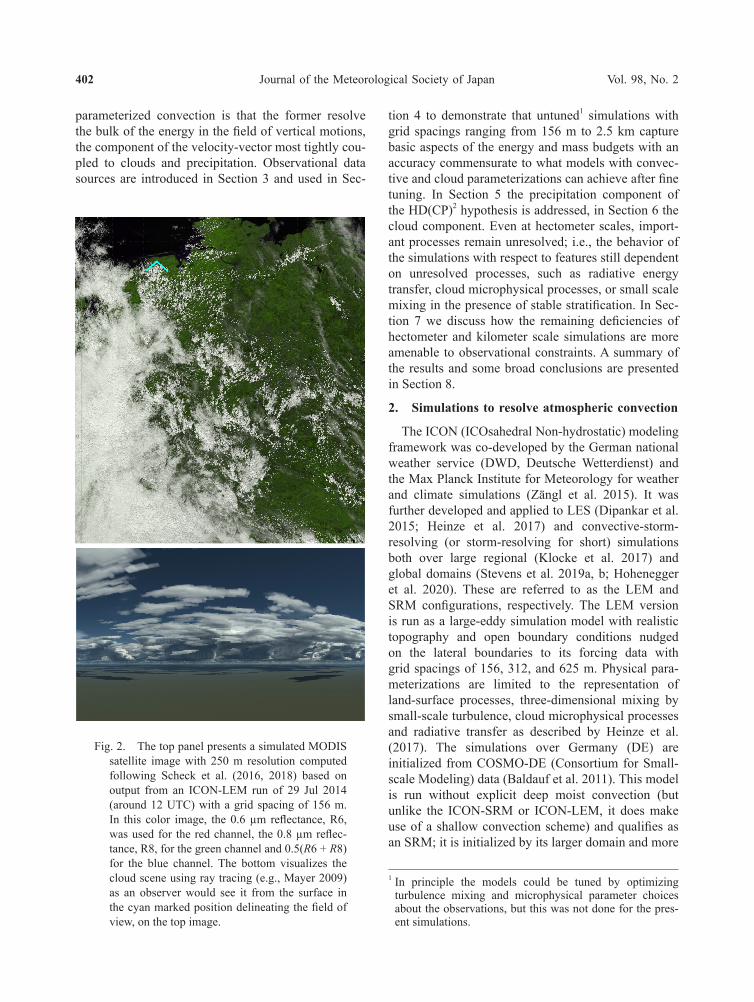
In the case of clouds, large-eddy simulations (LES) have long established the importance of hecto (and deca-) meter, and even finer (Mellado et al. 2018), scales. However, for reasons of computational ex-pense most LES have been performed for idealized situations, generally for short periods of time (hours) and over comparatively small (kilometers to tens of kilometers) domains (Moeng 1986; Siebesma et al. 2003; Rieck et al. 2012; Seifert et al. 2015). Even ap-proaches such as the LES ARM Symbiotic Simulation and observation workflow (LASSO) that are centered around intensive field measurements still adopt semi-idealized approaches using small domains that necessitate periodic boundary conditions (Fast et al. 2019). Super-parameterization has begun to allow a broader look at how an explicit representation of clouds couples to large-scale circulations (e.g., Paris-hani et al. 2018), but still using individual subdomains that remain small and idealized. The extent to which basic features of observed clouds, over large domains with realistic forcing and a realistic diel cycle, can be captured at hectometer scales has been much less explored. Our experience has been that the cloud-field can often be simulated in ways that appear quite real-
istic, for instance as illustrated by Fig. 2. Lacking is a more quantitative comparison. By simulating realistic cases, over large domains, the present study is able to use data over a wide variety of conditions to demon-strate the added value of kilometer and hectometer scale representations of clouds.
In an earlier paper, Heinze et al. (2017) described prototype simulations conducted at the end of the first phase of the HD(CP)2 project. Here we extend their analysis. The present approach differs from this and other scientific studies in that we make opportunistic use of a wide range of simulations, many performed for different specific purposes, in an attempt to distill more general insights. Some of the points we make, for instance, relating to the differences between para-meterized and explicit representations of convective precipitation, are less novel, but are presented to corroborate and extend the existing literature on the subject, also because the comparisons to measure-ments that are herein made, are in most cases new. Greater emphasis is placed on the study of cloud processes, as this work goes well beyond the state-of- the-art. The manuscript also emphasizes how sim-ulations of scales of motion comparable with those observed greatly enhance the bandwidth between the modeling and observational communities. This enriches the present analysis and provides a footing for better addressing some important deficiencies that even a global LES would not solve
The reference for the simulations, which are also archived and made available to the community for subsequent analysis, is found in Section 2. In this section it is argued that the distinction between storm-resolving simulations and approaches based on
Fig. 1. Visualization of convective processes associated with a frontal passage based on the output of the ICON-LEM model with 156 m grid spacing (top) and the ICON-NWP model run in the transpose AMIP mode with 40 km grid spacing (bottom) over Germany. Both simulations are for simulations of 24 April 2013. The colors denote ice (pink), liquid clouds (gray) and precipitation (blue).
Journal of the Meteorological Society of Japan Vol. 98, No. 2402
parameterized convection is that the former resolve the bulk of the energy in the field of vertical motions, the component of the velocity-vector most tightly cou-pled to clouds and precipitation. Observational data sources are introduced in Section 3 and used in Sec-
tion 4 to demonstrate that untuned1 simulations with grid spacings ranging from 156 m to 2.5 km capture basic aspects of the energy and mass budgets with an accuracy commensurate to what models with convec-tive and cloud parameterizations can achieve after fine tuning. In Section 5 the precipitation component of the HD(CP)2 hypothesis is addressed, in Section 6 the cloud component. Even at hectometer scales, import-ant processes remain unresolved; i.e., the behavior of the simulations with respect to features still dependent on unresolved processes, such as radiative energy transfer, cloud microphysical processes, or small scale mixing in the presence of stable stratification. In Sec-tion 7 we discuss how the remaining deficiencies of hectometer and kilometer scale simulations are more amenable to observational constraints. A summary of the results and some broad conclusions are presented in Section 8.
2. Simulations to resolve atmospheric convection
The ICON (ICOsahedral Non-hydrostatic) modeling framework was co-developed by the German national weather service (DWD, Deutsche Wetterdienst) and the Max Planck Institute for Meteorology for weather and climate simulations (Zängl et al. 2015). It was further developed and applied to LES (Dipankar et al. 2015; Heinze et al. 2017) and convective-storm- resolving (or storm-resolving for short) simulations both over large regional (Klocke et al. 2017) and global domains (Stevens et al. 2019a, b; Hohenegger et al. 2020). These are referred to as the LEM and SRM configurations, respectively. The LEM version is run as a large-eddy simulation model with realistic topography and open boundary conditions nudged on the lateral boundaries to its forcing data with grid spacings of 156, 312, and 625 m. Physical para-meterizations are limited to the representation of land-surface processes, three-dimensional mixing by small-scale turbulence, cloud microphysical processes and radiative transfer as described by Heinze et al. (2017). The simulations over Germany (DE) are initialized from COSMO-DE (Consortium for Small-scale Modeling) data (Baldauf et al. 2011). This model is run without explicit deep moist convection (but unlike the ICON-SRM or ICON-LEM, it does make use of a shallow convection scheme) and qualifies as an SRM; it is initialized by its larger domain and more
Fig. 2. The top panel presents a simulated MODIS satellite image with 250 m resolution computed following Scheck et al. (2016, 2018) based on output from an ICON-LEM run of 29 Jul 2014 (around 12 UTC) with a grid spacing of 156 m. In this color image, the 0.6 µm reflectance, R6, was used for the red channel, the 0.8 µm reflec-tance, R8, for the green channel and 0.5(R6 + R8) for the blue channel. The bottom visualizes the cloud scene using ray tracing (e.g., Mayer 2009) as an observer would see it from the surface in the cyan marked position delineating the field of view, on the top image.
1 In principle the models could be tuned by optimizing turbulence mixing and microphysical parameter choices about the observations, but this was not done for the pres-ent simulations.

B. STEVENS et al.April 2020 403
coarsely resolved counterpart COSMO-EU. For a de-tailed description of how ICON-LEM was configured and of how the simulations were performed, the reader is referred to the manuscript by Heinze et al. (2017).
The ICON-SRM version is run on 1.25 km and 2.5 km grid meshes. It differs from the ICON-LEM (as described by Heinze et al. 2017) in that the three-dimensional turbulence scheme is replaced by a boundary-layer parameterization and a turbulence mixing scheme that operates only on vertical columns. It differs from the ICON-NWP model in that it does not use parameterization for moist convection, and has no parameterization of shallow moist convection. The SRM uses the one-moment cloud microphysical scheme with graupel described by Baldauf et al. (2011), as also used by COSMO-DE. The SRM thus differs from the LEM that uses the two moment repre-sentation of cloud microphysics (Seifert and Beheng 2006). The initial and boundary data for the SRM are taken from the Integrated Forecasting System (IFS) of the European Centre for Medium-Range Weather Forecasts. Further details of the ICON-SRM as con-
figured for this study can be found in Klocke et al. (2017) and Hohenegger et al. (2020).
In addition, COSMO was used to provide an SRM reference for comparison to the LEM simulations over the DE domain. For these (what we call COSMO- SRM) simulations, boundary conditions and initial data were taken from COSMO-EU (or ICON-EU for the 2017 simulation). COSMO-SRM is very similar to the operational COSMO-DE model, whose output is used to initialize the ICON-LEM. The main differ-ences is that COSMO-SRM followed the LEM output protocol, and used the same two-moment microphys-ics used by the LEM, rather than the one-moment scheme used by COSMO-DE.
As simulations were being performed over a time period of approximately three years, bugs were iden-tified and resolved, so that different simulations were run with different code versions as improvements were incorporated. Important updates are noted in Table 1 which provides an overview of all the sim-ulations. The domains over which the simulations were performed and the number of simulated case
Table 1. Overview of models and periods for which simulations were performed and analyzed. Simulations on days marked with an asterisk (*) were performed with a model version with an erroneous calculation of the surface momentum trans-port. Set of convective days for calculating diurnal cycle over DE indicated by a text-dagger (†). See Fig. 3 for a geograph-ic specification of the simulation domains. Some DE simulations were shifted about one degree to the east with respect to the original domain, this shifted domain is not shown in Fig. 3. For limited area simulations, the lateral boundary condi-tions are taken from the same model as the initial conditions (IC).
Model, resolution - # level Domain IC/BCs Period Campaign/Qualification
ICON-LEM, 625 m, 312 m, 156 m - L150 DE COSMO-DE
20, 24–26* Apr, 2*, 5, 11*, 28 May 2013 HOPE
17 Jun, 29† Jul, 14†–15† Aug 201417 Jun, 4†–5 Jul 2015 shifted domain29 May, 3†, 6 Jun, 1 Aug, 2016, 22 Jun 2017
no accompanying global run
ICON-LEM, 625 m, 312 m, 156 m - L150 BB ICON-SRM
11, 12, 14–16, 20 Dec 2013 NARVAL 1 period10, 12, 17, 19, 22, 24 Aug 2016 NARVAL 2 period
ICON-SRM, 2.5 km, 1.3 km- L75 TA IFS
1 Dec 2013–31 Dec 2013 NARVAL 1 period1 Aug 2016–31 Aug 2016 NARVAL 2 period
ICON-SRM, 2.5 km - L75 NA IFS 21–25, 30 Sep, 1–5, 14–16 Oct 2016 NAWDEX period
ICON-SRM, 2.5 km - L75 MCEA IFS 26 Jun 2016–10 Jul 2016 30 May–6 Jul(extreme rain)
COSMO-SRM, 2.8 km - L50 DE COSMO-EU as ICON-LEM for DE domain see aboveICON-NWP, 40 km - L90 Global IFS as ICON-LEM and SRM no 2016 or 2017 DE daysICON-ECHAM, 40 km - L47 Global IFS as ICON-LEM and SRM no 2016 or 2017 DE daysECHAM, 100 km - L95 Global IFS as ICON-LEM and SRM no 2016 or 2017 DE days

Journal of the Meteorological Society of Japan Vol. 98, No. 2404
study days, analyzed in this manuscript, are presented with the help of Fig. 3 and Table 1. In some cases a simulated ‘day’ extends to 36 h or 48 h to follow the development of storms into the next day. Unless stated otherwise the analysis is performed for the finest reso-lution simulation on the given domain (Fig. 3).
To enable comparisons to simulations in which con-vection must be parameterized, additional simulations are performed with the global Numerical Weather Prediction (NWP) version of the ICON model, ICON-NWP, the climate model ECHAM6.3.02 (referred to as ECHAM hereinafter) which is the atmospheric component of the Max Planck Institute Earth System Model (Stevens et al. 2013) and ICON-ECHAM, which is the climate version of ICON using the ECHAM6 physics package (Giorgetta et al. 2018). ICON-NWP and ICON-ECHAM only share the same dynamical core and computational infrastructure, the ways in which subgrid-scale physical processes are parameterized differs substantially, also in terms of the applications for which they have been tuned. ICON-NWP was run with a grid spacing of 40 km. This particular resolution was chosen because it is com-parable to that of the finest resolution models used in the framework of the Coupled Model Intercomparison Project CMIP6 (Eyring et al. 2016), but significantly coarser than current operational global deterministic NWP system used by DWD, and for which the physics has been tuned. ECHAM was run with a spectral-triangular truncation of T127 that results
in 384 spectral-transform points along the equator, equivalent to approximately 100 km grid spacing. This resolution is state-of-the-art for decadal and centennial prediction systems. ICON-NWP, ICON-ECHAM and ECHAM were initialized by IFS data of the atmo-spheric and surface state and run forward in time for the same time-periods as indicated in Table 1. Running climate models as one would run a numerical weather prediction model, by initializing it with observed weather and analyzing its solutions on time-scales of hours to days, is known as Transpose AMIP (Williams et al. 2013). AMIP stands for the Atmospheric Model Intercomparison Protocol (Gates 1992), which eval-uates the climate of atmospheric models forced by specified sea-surface temperatures. The Transpose AMIP approach applied to the global models differs from the treatment of limited-area SRM and LEM simulations in that the latter are continually updated at their boundaries. For the quantities we look at, and given the size of the domain and the shortness of the simulations, we have no reason to believe that this makes a large difference, but it leads to a less ‘clean’ comparison and should thus be kept in mind.
The main difference between an SRM or LEM and conventional general circulation models (GCMs), which run at scales where convection has to be pa-rameterized, is that the former resolve dynamics in the third (vertical) dimension, i.e., the vertical motion and its variability. This is illustrated in Fig. 4, which illustrates the kinetic energy for the horizontal (Eu, v )
Fig. 3. Simulation domains as well as the number of simulated days for each domain, discussed in this paper. Storm- resolving simulation domains are depicted by a solid lime-green line (NA: Northern Atlantic, TA: Tropical Atlantic, MCEA: Maritime Continent East Asia), large-eddy simulation domains depicted by green lines (DE: Germany, BB: Barbados) solid for 156 m, fine-dashed for 312 m and coarse-dashed for 625 m grid spacings. Technical details for the model configuration for the simulations over each of these domains are provided in Table 1.
DEx20
NAx14
BBx12
TAx62
MCEAx15
Forced by TA
B. STEVENS et al.April 2020 405
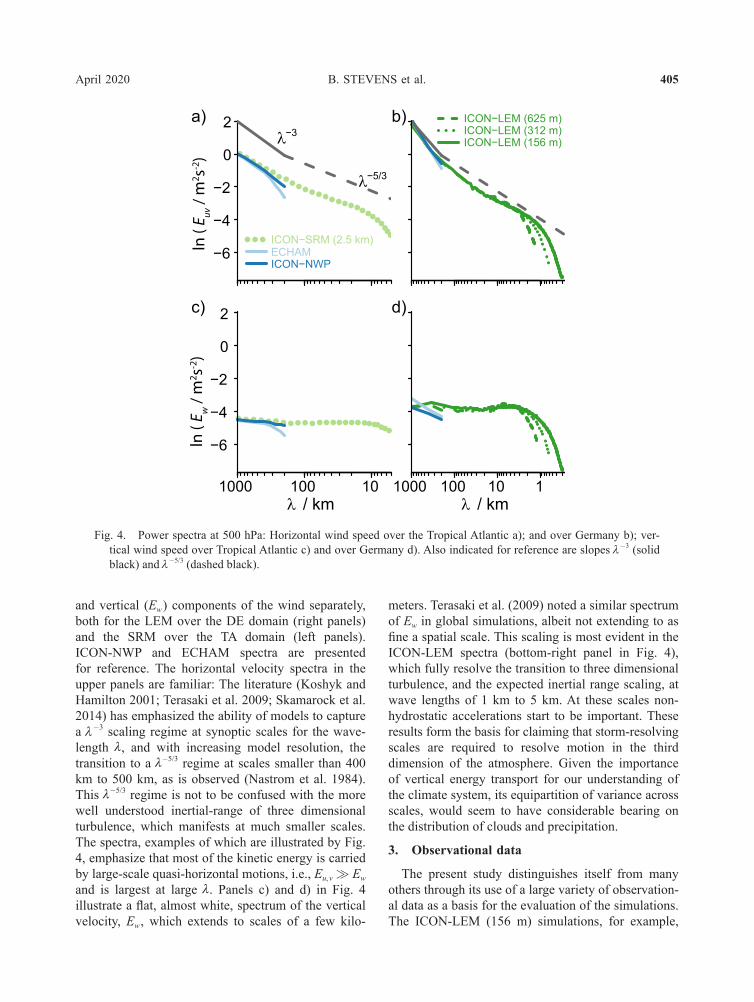
and vertical (Ew ) components of the wind separately, both for the LEM over the DE domain (right panels) and the SRM over the TA domain (left panels). ICON-NWP and ECHAM spectra are presented for reference. The horizontal velocity spectra in the upper panels are familiar: The literature (Koshyk and Hamilton 2001; Terasaki et al. 2009; Skamarock et al. 2014) has emphasized the ability of models to capture a λ-3 scaling regime at synoptic scales for the wave-length λ , and with increasing model resolution, the transition to a λ-5/3 regime at scales smaller than 400 km to 500 km, as is observed (Nastrom et al. 1984). This λ-5/3 regime is not to be confused with the more well understood inertial-range of three dimensional turbulence, which manifests at much smaller scales. The spectra, examples of which are illustrated by Fig. 4, emphasize that most of the kinetic energy is carried by large-scale quasi-horizontal motions, i.e., Eu, v Ew and is largest at large λ. Panels c) and d) in Fig. 4 illustrate a flat, almost white, spectrum of the vertical velocity, Ew , which extends to scales of a few kilo-
meters. Terasaki et al. (2009) noted a similar spectrum of Ew in global simulations, albeit not extending to as fine a spatial scale. This scaling is most evident in the ICON-LEM spectra (bottom-right panel in Fig. 4), which fully resolve the transition to three dimensional turbulence, and the expected inertial range scaling, at wave lengths of 1 km to 5 km. At these scales non- hydrostatic accelerations start to be important. These results form the basis for claiming that storm-resolving scales are required to resolve motion in the third dimension of the atmosphere. Given the importance of vertical energy transport for our understanding of the climate system, its equipartition of variance across scales, would seem to have considerable bearing on the distribution of clouds and precipitation.
3. Observational data
The present study distinguishes itself from many others through its use of a large variety of observation-al data as a basis for the evaluation of the simulations. The ICON-LEM (156 m) simulations, for example,
−6
−4
−2
0
2a)
−6
−4
−2
0
2
1000 10100λ / km
c)
b)
1000 10100 1λ / km
d)
λ−3
λ−5/3
ICON−LEM (625 m)ICON−LEM (312 m)ICON−LEM (156 m)
ln ( E u
v / m
2 s-2)
ln ( E w
/ m
2 s-2)
ECHAMICON−NWP
ICON−SRM (2.5 km)
Fig. 4. Power spectra at 500 hPa: Horizontal wind speed over the Tropical Atlantic a); and over Germany b); ver-tical wind speed over Tropical Atlantic c) and over Germany d). Also indicated for reference are slopes λ-3 (solid black) and λ-5/3 (dashed black).

Journal of the Meteorological Society of Japan Vol. 98, No. 2406
avail themselves to high-resolution measurements that capture even small-scale phenomena such as the ver-tical wind variances. The large domains, as employed for the Tropical Atlantic simulations, facilitate com-parisons with satellite data. In addition, model output is compared to ground-based networks of weather stations and active remote sensing instruments (radar and ceilometer networks). Data from three super sites located within the simulation domains: the Barbados Cloud Observatory (BCO, Stevens et al. 2016), the Jülich ObservatorY for Cloud Evolution (JOYCE-CF, Löhnert et al. 2015), and the Meteorologisches Obser-vatorium Lindenberg – Richard Amann-Observatorium (MOL-RAO, hereafter RAO) all provide detailed in-situ and remote-sensing data for comparison with the simulations. The HD(CP)2 Observational Proto-type Experiment HOPE (Macke et al. 2017) provided detailed cloud and precipitation measurements for a small region around Jülich (western part of Germany) with which the simulations can be evaluated. This also explains the cluster of simulations for the HOPE period in April and May 2013. Data from the Next Generation Remote Sensing for Validation Studies (NARVAL) flight campaigns (Stevens et al. 2019a) are incorporated for the analysis of the TA and Barbados (BB) simulations (see Fig 3), justifying the period chosen for these simulations. Simulations and mea-surements are compared for a 12-day period starting at 13 UTC on 10 Dec 2013, over a region of flight oper-ations (12°N to 17°N and 43°W to 63°W), that is even larger in size than the DE domain. Eight flights, each averaging approximately 8 h in duration, contribute to the composite cloud amount. Likewise the North Atlantic Waveguide and Downstream Impact Exper-iment (NAWDEX, Schäfler et al. 2018) anchors the NA simulations. Table A1 summarizes these diverse data sources, and their associated references.
For many of the data products, retrievals are applied to allow the comparison of remotely sensed quantities with physical properties simulated by the models. Cloud water path is retrieved from SEVIRI2 data uti-lizing the Cloud Physical Property retrieval developed by the Satellite Application Facility on Climate Moni-toring (CMSAF, Schulz et al. 2009). Liquid clouds are defined to be those with tops below 3.66 km, a value chosen based on the ECHAM vertical grid. Cirrus cloud cover is retrieved using the ‘Cirrus Properties from SEVIRI’ (CiPS) algorithm (Strandgren et al.
2017a, b). CiPS retrieves ice clouds using an artificial neural network trained with MSG/SEVIRI Infrared (IR) observations and corresponding cirrus properties derived from CALIPSO/CALIOP backscatter retriev-als. Validation against CALIOP indicates a very high sensitivity to thin ice clouds. The detection probability of ice clouds seen in CALIOP retrievals is 50, 60 and 80 % for cirrus with an optical thickness of 0:05, 0:08 and 0:14 respectively (Strandgren et al. 2017a), which corresponds to an Ice Water Path (IWP) of roughly 0.6, 1.0 and 3.0 g m-2, respectively.
4. Bulk statistics
Estimates of mean properties from simulations over the different domains were compiled along with refer-ence observations. These were intended to provide a quantitative overview of the different cases simulated, and the differences arising from different modeling frameworks. In cases where no direct measurements were available, ERA-Interim (Dee et al. 2011) data are used as a substitute for observational estimates. Sampling uncertainty is quantified through the stan-dard deviation of the simulation case (day) means for that domain. Values are tabulated as a reference for users of the output (Appendix and Tables A2 – 6). These statistics are indicative of how most of the simulations target situations where moist convection can be expected. Bowen ratios are generally less than 0.5, over the BB domain they are as low as 0.1. All domains, except for the NA, are also characterized by a net input of radiant energy at the top of the at-mosphere (TOA). In terms of mean temperatures, the simulations fall in two groups: MCEA, TA and BB have surface air temperatures near 300 K whereas the DE and NA domains are approximately 12 K colder. Precipitable, PW, varies from near 20 mm in the colder domains to 50 mm (MCEA). In a relative sense the NARVAL 1 simulations (BB) are the driest, with a PW of 30 mm but temperatures are much higher than in the NA or TA cases. The NARVAL 1 cases also have the lowest precipitation rate, near 1 mm d-1; the other domains have mean precipitation rates near 3 mm d-1, except for MCEA which has a domain mean precipitation rate approaching 6 mm d-1.
The compilation of mean statistics in Tables A2 – 6) aids an assessment of the extent to which LEM and SRM simulations stand out as compared to conven-tional models. In many cases the LEM and the SRM were run for the first time, whereas the global models have been developed over years and tuned to well represent climatological values. Despite this fact, the statistics tabulated in Appendix indicate no clear devi-
2 SEVIRI stands for the Spinning Enhanced Visible and Infrared Imager, which is carried by the geostationary Meteosat Second Generation (MSG) satellite.

B. STEVENS et al.April 2020 407
ation of the LEM or SRM simulations from the con-ventional models. In cases where the LEM or SRM is an outlier, it is not necessarily a worse fit to the observations (for instance, TOA shortwave irradiance over the MCEA domain). Looking across the simula-tions for general behavior there is some evidence that the SRM simulations are brighter (as measured by a smaller net shortwave irradiance at TOA), with larger liquid water paths, but less ice. This tendency is more evident for the SRM than for the LEM simulations, consistent with the former also being brighter, and with global SRM simulations as summarized by Stevens et al. (2019a, b).
5. Precipitation
As discussed in the introduction, a considerable literature demonstrates the ability of simulations with a grid spacing of a few kilometers to well represent precipitating deep convection. This literature empha-sizes the ability of such simulations to represent the structure of convective storms, particularly organized systems, as well as the frequency, intensity, and distri-bution of precipitation (Hohenegger et al. 2008; Prein et al. 2015; Kendon et al. 2017). Often it is concluded that grid-spacings of a few kilometers are adequate to capture the bulk statistics of precipitating deep convection (e.g., Langhans et al. 2012; Panosetti et al. 2019). These studies tend to emphasize case studies for a particular region; typically using a single model with grid-spacings that vary by a factor 4 – 10, with (and sometimes without) parameterized convection. When global domains are considered, the grid-spacing is often still somewhat coarse. In this section we ex-amine these questions from the perspective of a single modeling framework simulating cases from different climate regimes. We also compare our findings to global climate models with parameterized convection running at conventional (50 km to 100 km) grid spacings, hence containing little or no information associated with meso and storm-scale circulations.
We also explored new ground by analyzing simula-tions over large domains with much finer (hectometer) grid spacings. Where other studies have looked at the progressive impact of such finer scales, these tended to focus on idealized and isolated storms – the studies by Panosetti et al. (2019) and Langhans et al. (2012) being an exception – addressing particular questions, such as the most appropriate turbulent closure (Bryan et al. 2003), the role of non-hydrostatic accelerations (Jeevanjee 2017), and the effect of resolution on the effective buoyancy of convective plumes (Pauluis and Garner 2006). It is difficult to draw general
conclusions from convergence studies as conver-gence depends on the metric, and the models being investigated are asymptotically inconsistent (see e.g., Stevens and Lenschow 2001). Despite these reser-vations, the results from these convergence studies indicate that (i) there is a smooth transition between hydrostatic and non-hydrostatic regimes, and (ii) the misrepresentation of the relevant horizontal scales (in terms of the updrafts) is not as serious a challenge as previously believed, as there are signs of bulk conver-gence. As regards the former, cloud mixing processes may become Reynolds number invariant (converge) at tens of centimeters (Mellado et al. 2018), but higher order moments of this mixing process might only converge at smaller scales. The latter point refers to the failure of the models to asymptotically approach known fundamental laws as a control parameter (such as grid spacing) is refined. For example, as resolu-tion (or any other parameter) is refined, the cloud microphysical, land surface, or turbulent processes do not progressively approach known laws. For these reasons, the important question is how errors from the spatial truncation of the fluid motions compete with errors inherited from simplifications or uncertainties in the representation of other processes, such as the land surface, or microphysics; or how large do these errors end up being compared to those associated with alternative representations of convection.
5.1 The added value of hectometer grid spacingsTo address this question, we look both at the TA
simulations, over which cases were simulated with grid-spacings ranging between 312 m and 2500 m, and compare simulations with grid spacings ranging between 156 m and 625 m over the DE domain. The DE simulations have been run at yet coarser resolu-tions over a subset of cases, and the TA simulations have been performed at finer (156 m) grid-spacing over a smaller subdomain. In both cases we look for common changes in the structure, frequency, or intensity of the simulated fields of precipitation. In the simulations over the DE domain we additionally look for the signature of a better resolution of orographic effects as resolution is refined.
In a bulk sense, the simulations show some differences emerging from different configurations and/or from progressive refinement of simulations to hectometer scales. A signal of such differences is evident over the BB domain where the forcing is weaker, precipitation comes from shallower convec-tion, and conditions are more homogeneous. This is illustrated in Fig. 5, where we have computed the

Journal of the Meteorological Society of Japan Vol. 98, No. 2408
mean precipitation rate for a 21 h period between 15 UTC and 12 UTC. Starting at 15 UTC (six hours after initialization) avoids a pulse in precipitation that is evident in the nested (312 m to 625 m) simulations. The area of the spatial composite is chosen slightly smaller than the large BB domain (as depicted by the outer dashed line in Fig. 3) to avoid possible boundary effects. Time-series data (not shown) indicate that the differences in Fig. 5 are also apparent over the tempo-ral evolution, and thus appear systematic. Simulations with the smallest grid-spacing precipitate the least, but differ only slightly from those with a grid-spacing twice as coarse. The evolution with grid-spacing is not monotonic, simulations with Δ x = 1.25 km precipitate the most. Over the DE domain (not shown), there is also evidence of precipitation reducing as the grid encompasses hectometer scales, but these differences are less marked than they are for the BB domain. Bulk differences in precipitation between SRM and global (parameterized convection) simulations are larger over the TA domain than over the DE domain (compare Tables A2 and A4). We interpret these differences as evidence of a heightened sensitivity to resolution over the less strongly forced maritime conditions.
The similarity between the simulations at 625 m and 312 m over the BB domain is also evident in
the histogram of rain-rate intensity (Fig. 6a), and differs markedly from TA simulations with the 2.5 km ICON-SRM subsetted to the BB domain. The more coarsely resolved simulations appear to favor rain-rates with greater intensity. A similar comparison, this time between the LEM (625 m) and the COSMO- SRM (2.8 km) simulations over the DE domain (Fig. 6b), indicates that differences between the SRM and LEM representations of precipitation intensity are less marked over land – consistent with more con-sistent bulk statistics. The LEM also indicates more profound differences across domains than is evident for the SRM, something that is evident by comparing COSMO-SRM to ICON-SRM in Fig. 6b. These results suggest that the LEM distinguishes between the two convective regimes, with less frequent intense precipitation over the tropical ocean as compared to mid-latitude land, in ways that the SRM does not.
One interpretation of the reduction of precipitation as the mesh is refined to scales below 1.25 km is that smaller scale features contribute to the transport of condensate, and these are accelerated more rapidly for the same buoyancy perturbation (Pauluis and Garner 2006; Jeevanjee 2017). This would make them more susceptible to mixing and less efficient at producing precipitation. Simulations of a composite diel cycle by Panosetti et al. (2019) show a similar tendency, as do global simulations analyzed by Hohenegger et al. (2019), but the simulations by Bryan et al. (2003) in-dicate less of a clear relationship between the fineness of the grid mesh and the amount of precipitation.
A variety of attempts were made to identify signs of the land surface imprinting itself on precipitation more clearly as the grid spacing was refined to 156 m over the DE domain. None were successful. One idea was that mountain valley circulations would become more apparent, another idea was that the effect of coastlines, or landscape variability would become more evident, at these scales. Analysis of the experiments was unable to support such ideas. As part of a PhD project, Singh and Kalthoff (manuscript in preparation, 2019) examined these questions more systematically, by in-dependently varying the resolution of the land-surface representation and the model grid spacing. For the six cases they studied, the sensitivity to resolution was smaller than what we found over the TA domain, and the changes in the degree to which the land-surface is resolved contributed only 20 % to this change, the rest could be attributed to the effect of grid-spacing on the resolution of the atmosphere itself.
p312 / mm d-1
p Δx /
mm
d-1
ICON-SRM (1.25 km)
ICON-LEM (625 m)
ICON-SRM (2.5 km)
Fig. 5. Mean (15 UTC to 12 UTC the following day) precipitation, px as a function of Δ x versus the value at the finest grid-spacing ( p312 such that Δ x = 312 m) over the large BB domain. The SRM (1250 m and 2500 m grid spacing) simulations for the same days and averaged over the same BB domain are also included in the comparison.

B. STEVENS et al.April 2020 409
5.2 Large-scale structure and variability of precipitation
The ability of the storm-resolving model to capture the spatial distribution of precipitation is highlighted using output from the simulations over the MCEA and TA domains, as they provide a contrast to the varying influences on tropical precipitation. Mean pre-cipitation, as simulated by ICON-SRM and ECHAM, is compared to observations for the MCEA domain in Fig. 7 and for the TA domain in Fig. 8. The figures demonstrate that in quite different conditions the
freq
uenc
yfr
eque
ncy
COSMO-SRM (2.8 km)ICON-LEM (625 m)BB-ICON-SRM (2500 m)
a)
b)
BB DomainICON-SRM (2.5 km)ICON-LEM (625 m)
DE Domain
ICON-LEM (312 m)
10-1
10-3
10-5
0 50 100
10-1
10-3
10-5
p / mm h-1
Fig. 6. Histogram of non zero rain rates as a func-tion of their intensity for ten days over the large (312 m) BB domain (11, 12, 14, 15, and 20 Dec 2013 and 10, 12, 19, 22, and 24 Aug 2016), panel a; and for 16 days over the DE domain (20, 24 – 26 April, and 5 May 2013, 17 Jun, 7 Jul, and 14, 15 Aug 2014, 17 Jun, and 4, 5 Jul, 2015, 29 May, 6 Jun, and 1 Aug 2016, and 22 Jun 2017), panel b. Illustrated are results from grids with different grid spacings, whereby counts are computed after gridding all output to a coarser (7 km) grid to avoid grid-point effects.
c) ECHAM
b) ICON-SRM (2.5 km)
a) OBS
10 ºS
10 ºN
30 ºN
10 ºS
10 ºN
30 ºN
10 ºS
10 ºN
30 ºN
90 ºE 120 ºE 150 ºEp / mm d-1
Fig. 7. Daily mean precipitation for the simulation period (26 Jun 2016 – 10 Jul 2016) of MCEA (mm d-1). Observations (CMORPH satellite and rain gage (over land) merged precipitation prod-uct within and GPM outside dashed box), ICON-SRM and ECHAM remapped to a 1° × 1° grid. The solid black line bounds a region of extreme rainfall wherein satellite and surface analyses are merged.
Journal of the Meteorological Society of Japan Vol. 98, No. 2410
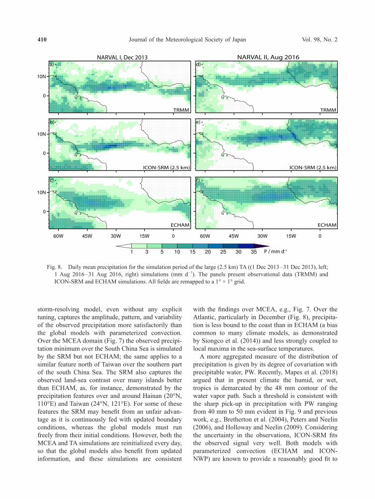
storm-resolving model, even without any explicit tuning, captures the amplitude, pattern, and variability of the observed precipitation more satisfactorily than the global models with parameterized convection. Over the MCEA domain (Fig. 7) the observed precipi-tation minimum over the South China Sea is simulated by the SRM but not ECHAM; the same applies to a similar feature north of Taiwan over the southern part of the south China Sea. The SRM also captures the observed land-sea contrast over many islands better than ECHAM, as, for instance, demonstrated by the precipitation features over and around Hainan (20°N, 110°E) and Taiwan (24°N, 121°E). For some of these features the SRM may benefit from an unfair advan-tage as it is continuously fed with updated boundary conditions, whereas the global models must run freely from their initial conditions. However, both the MCEA and TA simulations are reinitialized every day, so that the global models also benefit from updated information, and these simulations are consistent
with the findings over MCEA, e.g., Fig. 7. Over the Atlantic, particularly in December (Fig. 8), precipita-tion is less bound to the coast than in ECHAM (a bias common to many climate models, as demonstrated by Siongco et al. (2014)) and less strongly coupled to local maxima in the sea-surface temperatures.
A more aggregated measure of the distribution of precipitation is given by its degree of covariation with precipitable water, PW. Recently, Mapes et al. (2018) argued that in present climate the humid, or wet, tropics is demarcated by the 48 mm contour of the water vapor path. Such a threshold is consistent with the sharp pick-up in precipitation with PW ranging from 40 mm to 50 mm evident in Fig. 9 and previous work, e.g., Bretherton et al. (2004), Peters and Neelin (2006), and Holloway and Neelin (2009). Considering the uncertainty in the observations, ICON-SRM fits the observed signal very well. Both models with parameterized convection (ECHAM and ICON-NWP) are known to provide a reasonably good fit to
NARVAL I, Dec 2013 NARVAL II, Aug 2016a)
b)
c)
d)
e)
f )
P / mm d-1
TRMM
ICON-SRM (2.5 km)
ECHAM
TRMM
ICON-SRM (2.5 km)
ECHAM
Fig. 8. Daily mean precipitation for the simulation period of the large (2.5 km) TA ((1 Dec 2013 – 31 Dec 2013), left; 1 Aug 2016 – 31 Aug 2016, right) simulations (mm d-1). The panels present observational data (TRMM) and ICON-SRM and ECHAM simulations. All fields are remapped to a 1° × 1° grid.

B. STEVENS et al.April 2020 411
the observations and this is evident in Fig. 9; even so, both indicate more precipitation at lower values of PW as compared to ICON-SRM. Rain-rates are twice the observed (or SRM simulated) value in the critical range of the precipitation transition between column water vapor amounts of 40 mm to 50 mm. For high values of column water vapor, the SRM simulates a mean precipitation rate higher than reported by the observations.
Not all aspects of the SRM precipitation are clear improvements. The simulations at storm-resolving scales produced intense precipitation in certain coastal regions that appear well in excess of what is derived from the Tropical Rainfall Measuring Mission (TRMM) Multisatellite Precipitation Algo-rithm (TMPA; Huffman et al. 2007), although one should also bear in mind possible limitations in the observations, especially in regions of complex terrain. Differences with TRMM are evident along the coast of Myanmar and Thailand (Fig. 7) and along the coast of West Africa (near Guinea) in boreal summer (Fig. 8). A similar issue is evident in the NA simulations (not shown) along the west coast of South Greenland. In every case the observations have signs of a similar local maximum, but not as pronounced. In most cases local maxima are not present on the coasts in the sim-ulations with parameterized convection. For instance, Fig. 7 illustrates how precipitation maximizes off shore over the Bay of Bengal in the simulations with
ECHAM.In addition to a generally better spatial distribution,
precipitation features simulated by the SRM have a more realistic signature of spatial variability than is evident in the simulation with parameterized convec-tion. This is highlighted in the Hovmöller diagram (Fig. 10) showing the latitudinal (28 – 32°) averaged precipitation rate in the boxed region of Fig. 7. Dam-aging floods affected this region during the simulated period in connection with the quasi-stationary Mei-yu front, with precipitation totals of 193 mm recorded over a seven day period (between 30 Jun and 6 Jul 2016). Accumulated precipitation in the SRM simula-tions totaled 186 mm. The models with parameterized convection produced 137 mm (ICON-ECHAM) and 143 mm (ICON-NWP). Although it is difficult to rule out chance in the ability of the SRM to better repre-sent the higher precipitation amounts, this improve-ment coincides with a better representation of the structure and evolution of the responsible storms. This is evident through the eastward migration of storms over the flooded region in the SRM, which is largely absent in the models with parameterized convection for which precipitation appears more diurnally driven and spatially locked (Fig. 10). Likewise, over Africa, the lack of large-scale propagating features and a too strong diel cycle (Fig. 11) leads to a too low day-to-day variability in ECHAM. This can be quantified using the coefficient of variation of the temporal variability (the ratio of the standard deviation to the mean), which we have calculated for the domain- average of the west African Sahel, where variability plays an important role. The observed value is 2.1, compared to 1.4 in ICON-ECHAM and 1.7 in ICON-SRM. Though still varying less than observed, this bias is reduced by nearly a factor of two in the SRM. The ability of storm-resolving models to better rep-resent meso-scale convective systems over Western Africa has also been noted by earlier studies (e.g., Pearson et al. 2014; Beucher et al. 2014; Maurer et al. 2015; Zhang et al. 2016; Peters et al. 2019).
5.3 Diel cycle of precipitationThe fact that precipitation peaks in the late-af-
ternoon or early-evening over tropical continents is known for some time, e.g., observations over Sudan (Pedgley 1969) and over Northeast Brazil (Kousky 1980). Additionally over mid-latitude continental areas, the late-afternoon peak is so well known as to feature in children’s books romanticizing a lazy summer day (Stietencron 1992). The failure of con-vective parameterization to capture this signal was
P / m
m d
-1
PW / mm
ICON-SRM (2.5 km)
ECHAM
OBS
ICON-NWP
Fig. 9. Mean precipitation rate (P) over the ocean as a function of precipitable water (PW) for ob-servations (HOAPS), ECHAM, ICON-NWP and ICON-SRM (2.5 km) over the large TA domain for full period (1 Dec 2013 – 31 Dec 2013). All data were coarse grained to the resolution from ECHAM before the dependency was calculated and only water vapor bins with ten values or more are considered.

Journal of the Meteorological Society of Japan Vol. 98, No. 2412
Fig. 11. Hovmoeller plot of latitudinal averaged precipitation rate (2°S – 16°N, mm d-1) over the tropical Atlantic during August 2016. Observations (IMERG) illustrated in a), ICON-SRM in b), and ECHAM c).
Augu
st /
d
1
7
14
21
28
60 W 30 W 0 60 W 30 W 0 60 W 30 W 0
a) Obs b) ICON-SRM (2.5 km) c) ECHAM
0.5 1 1.5 2 2.5 3 4 5 10 P / mm d-1
Fig. 10. Hovmöller plot of latitudinal averaged precipitation rate (mm h-1; 28 – 32°N, see black box in Fig. 7) for an extreme monsoon event in east China (30 Jun 2016 until 6 Jul 2016), for longitude values from 100 – 125°E, see black box in Fig. 7. Observations (CMORPH satellite and rain gage merged precipitation product) illustrated in a), ICON-SRM (2.5 km) illustrated in b) and ECHAM c). Gray dashed lines indicate local noon.
a) OBS b) ICON-SRM (2.5 km) c) ECHAM
100 ºE 120 ºE 100 ºE 120 ºE 100 ºE 120 ºE
1
3
5
0.5 1 1.5 2 2.5 3 4 5 6 P / mm h-1
July
/ d
B. STEVENS et al.April 2020 413
also identified long ago (Dai et al. 1999). Although a few groups have demonstrated an ability to capture such a signal (Takayabu and Kimoto 2008; Hourdin et al. 2013; Bechtold et al. 2014), progress is spotty and large errors continue to persist over many genera-tions of model development (Covey et al. 2016). Over land, precipitation is too coherent with the phase and amplitude of the diel cycle in these models. By con-trast, storm-resolving models, even with grid spacings as coarse as 7 km to 14 km, are able to represent the observed signal of diurnal variability in locally forced
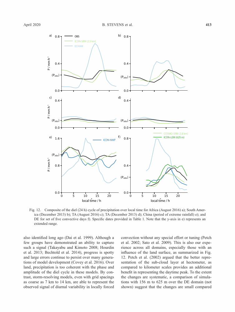
convection without any special effort or tuning (Petch et al. 2002; Sato et al. 2009). This is also our expe-rience across all domains, especially those with an influence of the land surface, as summarized in Fig. 12. Petch et al. (2002) argued that the better repre-sentation of the sub-cloud layer at hectometer, as compared to kilometer scales provides an additional benefit in representing the daytime peak. To the extent the changes are systematic, a comparison of simula-tions with 156 m to 625 m over the DE domain (not shown) suggest that the changes are small compared
Fig. 12. Composite of the diel (24 h) cycle of precipitation over local time for Africa (August 2016) a); South Amer-ica (December 2013) b); TA (August 2016) c); TA (December 2013) d); China (period of extreme rainfall) e); and DE for set of five convective days f). Specific dates provided in Table 1. Note that the y-axis in e) represents an extended range.
ICON-SRM (2.5 km)
ECHAM
ICON-LEM (625 m)
OBS
ICON-NWP
COSMO-SRM (2.8 km)
local time / h local time / h
c) d)
a) b)
e) f )
P / m
m h
-1P
/ mm
h-1
P / m
m h
-1

Journal of the Meteorological Society of Japan Vol. 98, No. 2414
to the differences between parameterized and explic-itly represented precipitation in our simulations. This finding is consistent with the composite diel cycles simulated by Panesotti et al. (2019) who considered values of Δ x ranging from 550 m to 8800 m.
Some of the challenges of convective parameter-ization, as well as associated advantages of resolving deep convection, are illustrated by the simulations of the diel cycle over Germany. Figure 12f presents the composite diel cycle for days with summer conditions and largely locally forced precipitation (29 Jul, 14 – 15 Aug 2014, 4 Jul 2015, and 3 Jun 2016). For these days and region, ECHAM produces a diel cycle with rainfall peaking near noon and absent at night; this is consistent with errors evident in more tropical regions (panels a, b and e), which are typical of most climate models (e.g., Covey et al. 2016). By contrast, ICON-NWP, which uses the convection scheme developed at ECMWF (Bechtold et al. 2014) and is exemplary of models with state-of-the-art convective parameterization that have been developed to address the bias in the diel cycle of precipitation, has much smaller systematic errors in its representation of the diel cycle (panel f). However, even in the ICON-NWP simulations, precipitation still peaks too early and decays too strongly as the sun retreats. The better simulation of night-time precipitation by the LEM, as compared to the best performing model with con-vective parameterization, is evident by its ability to produce substantial (and more intense) precipitation falling after 2000 UTC, which is similar to what was observed. In addition to the total amount of precip-itation, the distribution of precipitation rates is im-proved by LEM. This is illustrated in Fig. 13, where the relative rain fraction asymptotes to the fraction of the observed precipitation that is simulated. The flatness of the curves for ECHAM (P > 2 mm h-1) and ICON-NWP (P > 3.5 mm h-1) is indicative of a lack of more intense precipitation in the models with parameterized convection. Although not illustrated in the figure, because deviations are too small compared to the differences to the other models, there is a slight tendency for the LEM to better match the observations as its grid-spacing is refined from 625 m to 156 m. A systematic early decline in night-time precipitation was also noted in convection permitting simulations centered over Germany by Rasp et al. (2018), which were performed with the COSMO model on a grid of 2.8 km for 26 May to 9 June 2016. This suggests that for precipitation, the added value of the LEM, as compared to the SRM, might be more evident at night.
6. Clouds
For the evaluation of clouds we used simulations over the DE domain to take advantage of a dense network of observations collected over Germany (Lammert et al. 2019), spanning an area of 360000 km2. Simulations on the TA and BB domains enable comparisons with aircraft observations from the NARVAL expeditions (Stevens et al. 2019a, b) and ongoing measurements from the Barbados Cloud Observatory (Stevens et al. 2016). Over the TA/BB domain the spatial sparseness of the observations poses greater challenges for the model evaluation, notwithstanding surface conditions considerably more homogeneous than those over the DE domain.
6.1 Statistical signature of clouds over the DE domain
a. Cloud condensate distributionBy virtue of its close connection to cloud opti-
cal thickness, condensate water path (CWP) links strongly to the radiative effects of clouds (Stephens 1978; Harshvardhan and Espinoza 1995). Figure 14a presents the cumulative distribution of CWP for ICON-LEM, ECHAM and ICON-NWP, with measurements from all available twenty-two MODIS3
Fig. 13. Night time (20 – 24 UTC) relative rain fraction over precipitation rate for five convective days (see Table 1) in the DE domain. The relative rain fraction is calculated by dividing the amount of precipitation contributed by rain rates smaller or equal to a given precipitation rate by the total precipitation amount found in the observations. Observational data is taken from the RADOLAN network. As in Fig. 12f, only the set of convec-tive days is considered (as in Fig. 12).
3 MODIS stands for the Moderate-resolution Imaging Spec-troradiometer, which flies on the NASA Aqua and Terra satellites.
frac
tion
P / mm h-1
0
1
0 5
ECHAMICON-NWP
RADOLAN
ICON-LEM (625 m)

B. STEVENS et al.April 2020 415
overpasses taken from eight simulation days and from the SEVIRI. SEVIRI’s footprint is as much as twenty times coarser than MODIS (1 km2 at nadir). To ensure some degree of homogeneity only MODIS pixels with viewing angles within 40° off nadir were selected, and to avoid biases from the limited sensitivity of the instruments a detection threshold of CWP < 10 g m-2 was applied. Because the retrievals use measurements of reflected sunlight the comparison is done for day-time only. Similar filtering is applied on ICON and ECHAM simulations that are geographically matched (through the nearest neighbor) to the spatial and temporal footprint of the satellite. Temporal matching is ±150 s for ICON-LEM, and ±1800 s for ECHAM and ICON-NWP, whose CWP output is hourly. Figure 14 indicates that ICON-LEM is in close agreement with MODIS (for CWP > 100 g m-2) the instrument to which its resolution is most commensurate, albeit with a greater contribution from low CWP than seen
by MODIS. Less agreement at lower CWP may be a shortcoming of the simulations, or indicative of limitations in the sensitivity of MODIS to clouds that are optically thin or composed of very small droplets; small CWP values may also contain a non-negligible contribution from thin ice clouds in single- or multi- layer conditions, which are poorly treated by MODIS retrievals (Sourdeval et al. 2016).
Differences between the MODIS and MSG retriev-als (as presented in Section 3) are expected as a result of differences in sensor footprints. The much larger MSG footprint effectively smooths the CWP field, leading to lower values, and introduces systematic biases due to heterogeneity effects as discussed by Heinze et al. (2017). This is consistent with MSG re-trievals better matching to the lower resolution models (ICON-NWP and ECHAM). However, given that both ICON-NWP and ECHAM have grid cells much coars-er than even the MSG footprint, the tendency of their cumulative distributions to lie between that of MODIS and MSG is indicative of a bias. If their CWP were consistent with the observations one would, by virtue of their coarser resolution, expect the distribution to shift to smaller values than those measured by MSG. The lack of such a shift implies clouds that are on average too bright. Simulating too much condensate has the beneficial effect of compensating systematic biases arising from a failure to account for sub-grid heterogeneity so as to still get the correct irradiance at TOA. Earlier studies, using very different methods, came to similar conclusions, for example Nam et al. (2012). The smoothing effect of off-nadir retrievals may also explain the discrepancy between the LEM and MODIS. It certainly seems plausible that the LEM would still under-represent the optically thinnest clouds, but at a first look, the agreement between the observations of CWP and the LEM output agreed.
The distribution of the liquid water path is com-pared with the observations in Fig. 14b. For this analysis, the ICON-LEM low-level cloud LWP is coarse-grained to the MSG grid and a detection threshold of LWP < 1 g m-2 is applied. Only values during daytime (between 6 UTC and 18 UTC for the days investigated) were analyzed. The peak at LWP » 1000 g m-2 in ICON-NWP is caused by one day (29, Jul 2014) in association with a severe storm. Given the five-hundred fold difference in the MSG versus ECHAM footprint, the lack of a shift in the ECHAM LWP distribution toward low values relative to MSG is also indicative of the parameterized clouds in both models being too bright. ICON-LEM using samples coarse-grained to the MSG footprint is more consis-
Fig. 14. Cumulative density function of CWP a); and probability density function of the liquid water path (LWP), b), retrieved by satellite (MSG: solid black line; MODIS: dashed black line) and simulated by ICON-LEM, ICON-NWP, and ECHAM. Note, that for ICON-LEM in panel a), results are presented at the MODIS resolution, while for panel b), results are presented at the optical resolution of MSG (coarse-grained field).
(156 m)
p(LW
P)
0.0
0.1
0.2
0.3
C(CW
P)
100 101 102 103 104
100 101 102 103 104
CWP / gm-2
LWP / gm-2
0
1a)
b)

Journal of the Meteorological Society of Japan Vol. 98, No. 2416
tent with the observations.
b. Profi les of cloud coverTo evaluate vertical cloud fraction profi les we fi rst
use super site measurements from JOYCE-CF in the west of Germany and from RAO, near Poland, in east-ern Germany. Comparisons are made between 6 UTC and 0 UTC to avoid problems with the model spin-ups during the fi rst six hours of the simulations. Observed cloud profi les are based on the Cloudnet target classi-fi cation following Illingworth et al. (2007). Compar-ing spatially averaged fi elds to point measurements is an imperfect exercise. However, large qualitative differences emerge between the observed profi les and those produced by the models for which clouds are parameterized (Fig. 15). Both the SRM (COSMO-DE) and the LEM better represent the structure of the observed profi les, with a double maximum with peak coverage in the lower (near 3 km) and upper (near 9 km) troposphere. Quantitatively the LEM produces substantially few clouds, in better accord with the observations. Hentgen et al. (2019) similarly found an
over-prediction of clouds at mid-levels in simulations using COSMO over Europe. For high cloud cover (above 10 km) ICON-LEM and the SRM (COSMO-DE) produce too much cloud-cover compared to the coarser models and the observations. The color shaded areas in Fig. 15 delineate the range of profi les obtained by varying the threshold of IWP required to identify a scene as cloudy. The region of shading thus demonstrates that ECHAM’s and ICON-NWP’s sen-sitivities to thin ice clouds are mostly manifest above 6 km and that ICON-LEM simulates a larger fraction of optically thin cirrus and ice clouds in general.
Poor accounting of spatial variability limits one’s ability to draw strong conclusions from the above analysis. In an effort to partially address this short-coming the coverage of ice-clouds is also compared to cloud cover derived from satellite using the CiPS re-trieval (as described in Section 3). Figure 16 indicates that the CiPS derived cirrus cloud cover frequency distribution is largest for low coverage and drops for increasing cover, a quality represented by all models. The frequency distribution of ice cloud cover simu-
Fig. 15. Comparison of average cloud cover profi les for six simulated days. Vertical profi les display mean values between 6 UTC and 24 UTC comparing different simulations to profi les obtained from cloud radar observations from the two super sites located in West (JOYCE-CF) and North-East (Lindenberg) Germany. Color shaded areas for model outputs represents the sensitivity to different IWP thresholds, while grey shaded area shows the mean difference between the two measurement sites.
Fig. 16. Frequency diagram of fractional cirrus cloud cover over Germany from CiPS (Cirrus Properties from SEVIRI), ICON-LEM, ICON-NWP and ECHAM. High cloud cover fractions were calculated using 3 different ice water path thresholds, 0.6, 1, and 3 g m-2, which are associ-ated with a cirrus cloud cover detection effi ciency by CiPS of about 50, 60, and 80 %, respectively. The shaded areas for the different models indicate the uncertainty of cirrus cloud coverage assum-ing those 3 detection sensitivities.
heig
ht /
km
amount / %0 10 20
6
12
0
ICON-LEM (156 m)COSMO-SRM (2.8 km)ICON-NWPECHAMOBS
ICON-LEM (156 m)
ICON-NWPECHAM
OBS
freq
uenc
y
high cloud-cover0 10
0.5

B. STEVENS et al.April 2020 417
lated by the LEM is flatter and aligns more closely with the CiPS retrievals than the other models do. The shaded areas show the variation in cirrus cloud frac-tion due to the different IWP thresholds (following the detection probability of CiPS) as applied to the model output. This analysis also reaffirms the inference from the previous figure (Fig. 15), whereby the ice-cloud coverage in the LEM samples more thin ice-clouds than the models with parameterized convection. Dif-ferent microphysical parameterizations are likely to also play a role, which makes it difficult to attribute the better performance of the LEM only to its ability to explicitly represent the condensate transport.
c. Cloud base height evaluationCloud-base height has a strong influence on down-
welling long-wave radiation at the surface, and hence, on the surface energy budget. Figure 15 suggests that cloudiness near the cloud base (between 1 km and 2 km) simulated by the LEM is less (by as much of a factor of two) than observed, whereas ICON-NWP agrees well with the observations. ICON-LEM
features fog and low stratus over the marine coastal regions on approximately half of the simulated days. This peak is not represented in ceilometer observa-tions because they are situated over land. Above 3 km the situation is reversed, with the LEM better representing the coverage of mid to high-clouds, as discussed in the previous section (6.1b). The apparent-ly deficient representation of low clouds by the LEM may be misleading however, as low-clouds are more strongly tied to surface features and thus more likely to be biased by poor sampling. When compared to 155 ceilometer stations evenly distributed over Germany (Kotthaus et al. 2016; Wiegner et al. 2014), the LEM cloud-base heights are more uniformly distributed be-tween 0.5 km and 4 km and in better agreement with the observations, particularly in the afternoon and early evening after the convective boundary layer has been established (Fig. 17). ICON-NWP, by contrast accumulates cloud bases near 1 km, consistent with its peak in cloudiness at this level in Fig. 15.
The ceilometer data also provide an opportunity to study how cloud-base evolves over the day. Ceilo-
Fig. 17. Diel cycle of mean cloud-base height calculated by selecting only cloud base heights below 4 km from 155 ceilometer stations of the DWD ceilometer network and ICON-LEM (156 m), ICON-NWP, and ECHAM over Germany. Morning (06 – 12 UTC) profiles, a); afternoon (12 – 18 UTC) profiles, b); evening (18 – 24 UTC), c); diel cycle, d).
0
1
2
3
4z cb
/ km
z cb / k
m
0.9
1.5
2.1
.04 .080 .04 .080 .04 .080
a) b) c)
d)
p(zcb) / mp(zcb) / m p(zcb) / m
6 12 UTC time / h
06-12 UTC 12-18 UTC 18-24 UTC
Obs (ceilometer network)
ICON-LEM (156 m)ICON-NWP
ECHAM
18

Journal of the Meteorological Society of Japan Vol. 98, No. 2418
meter measurements over Germany indicate a distinct diurnal cycle in cloud base height, with cloud base rising through the afternoon and peaking in the late afternoon or early evening (local time leads UTC by 20 min to 60 min). Both ICON-LEM and ECHAM capture the diurnal signature of the ceilometer measurements, but ICON-LEM better represents its amplitude and phase. The slight lead in the phase of the ICON-LEM relative to the ceilometer measure-ments is also seen in the development of boundary layer clouds over the JOYCE-CF (Acquistapace et al. Boundary layer cloud life cycle in ICON-LEM and ground-based observations, manuscript in preparation) and may be rooted in a too rapid re-establishment of a deep convective boundary layer in the morning.
The ceilometer measurements have also been used to test the representation of cloudiness duration statistics. The length of contiguous cloud-base height returns at individual instruments provides a measure of cloud size statistics. The ICON-LEM captures the roughly exponential distribution of observed cloud du-ration, becoming increasingly flat and in better accord with the observations as Δ x is reduced (Fig. 18). Thus the frequency of short events increases at the expense of longer events as grid spacing is refined. Short-lived clouds are simulated at the highest model resolution as frequently as observed, and the bias toward more long-lived clouds is reduced with increasing resolu-tion.
The preceding discussion demonstrates that even for a well instrumented, and relatively homogeneous region, such as Germany, a definitive evaluation of simulated cloud statistics is difficult. Nonetheless we venture some conclusions. Overall, the ICON-LEM produces a more compelling representation of the cloud field than the models that must parameterize the scales of motion to which clouds respond. Despite some deficiencies in the way clouds are calculated in ICON-LEM, their representation is expected to improve with finer resolution. This seems trivial, but when one reflects on the construction of models with parameterized convection, whose parameterizations act independently in each grid box or column, it quick-ly becomes clear that convergence is a more intrinsic property of the LEM and SRM approach. Barring a few notable and increasingly anachronistic exceptions, e.g., simple statistical approaches as in Sommeria and Deardorff (1977), models with parameterized clouds lack this property, as when cloud are parameterized, every different resolution defines a different model.
6.2 Representation of clouds over the TA domainThe wide variety of cases simulated in the HD(CP)2
project allows us to contrast the simulation of clouds over Germany with those over the tropical oceans. For this purpose we make use of a special dataset with long-term surface observations at the Barbados Cloud Observatory (Stevens et al. 2016) and airborne measurements from two field campaigns (Stevens et al. 2019a). In analogy to Fig. 15, Fig. 19 presents a comparison of the simulated cloud amount profile with measurements from a nadir staring cloud radar deployed from the high-altitude research aircraft High Altitude and Long Range Research Aircraft (HALO). The analysis suggests that the models with parame-terized convection underestimate the amount of low clouds and over-estimate the coverage of high-clouds and that ICON-LEM is in better accord with the mea-surements. When neglecting ice clouds with ice water paths below 3 g m-2, the upper level cloud amount is substantially reduced. Nevertheless, the fraction of opaque cirrus clouds for ICON-NWP and ECHAM still exceeds the total cirrus cloud fraction of ICON-SRM including thin cirrus. This finding is consistent with that of Cesana and Waliser (2016) who found that large-scale models with parameterized clouds overes-timate high-cloud frequency and vertical extent. All models miss the local cloud-amount maximum near 9 km; this is thought to reflect chance detrainment from a nearby deep convective cloud on one of the flights,
Fig. 18. Normalized frequency of occurrence of cloud lifetime densities for low-level (< 3 km from cloud base) clouds under scattered and broken cloud conditions (i.e. cloud cover between 25 % and 87 %) of 6 days. Cloud lifetimes ob-served by the DWD ceilometer network in Ger-many (black) and as simulated by ICON-LEM.
cloud lifetime / min
freq
uenc
y /
%
ICON-LEM (156 m)ICON-LEM (312 m)ICON-LEM (625 m)
OBS
102
101
100
10-1
10 200 30
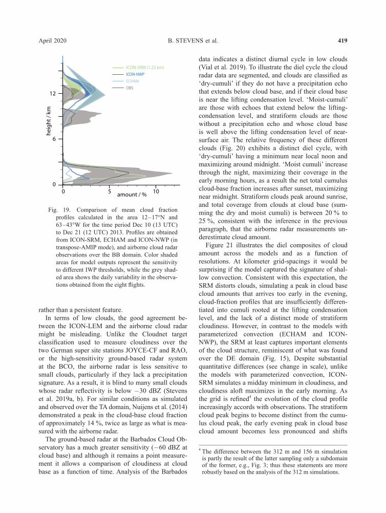
B. STEVENS et al.April 2020 419
rather than a persistent feature.In terms of low clouds, the good agreement be-
tween the ICON-LEM and the airborne cloud radar might be misleading. Unlike the Cloudnet target classifi cation used to measure cloudiness over the two German super site stations JOYCE-CF and RAO, or the high-sensitivity ground-based radar system at the BCO, the airborne radar is less sensitive to small clouds, particularly if they lack a precipitation signature. As a result, it is blind to many small clouds whose radar refl ectivity is below -30 dBZ (Stevens et al. 2019a, b). For similar conditions as simulated and observed over the TA domain, Nuijens et al. (2014) demonstrated a peak in the cloud-base cloud fraction of approximately 14 %, twice as large as what is mea-sured with the airborne radar.
The ground-based radar at the Barbados Cloud Ob-servatory has a much greater sensitivity (-60 dBZ at cloud base) and although it remains a point measure-ment it allows a comparison of cloudiness at cloud base as a function of time. Analysis of the Barbados
data indicates a distinct diurnal cycle in low clouds (Vial et al. 2019). To illustrate the diel cycle the cloud radar data are segmented, and clouds are classifi ed as ‘dry-cumuli’ if they do not have a precipitation echo that extends below cloud base, and if their cloud base is near the lifting condensation level. ‘Moist-cumuli’ are those with echoes that extend below the lifting-condensation level, and stratiform clouds are those without a precipitation echo and whose cloud base is well above the lifting condensation level of near-surface air. The relative frequency of these different clouds (Fig. 20) exhibits a distinct diel cycle, with ‘dry-cumuli’ having a minimum near local noon and maximizing around midnight. ‘Moist cumuli’ increase through the night, maximizing their coverage in the early morning hours, as a result the net total cumulus cloud-base fraction increases after sunset, maximizing near midnight. Stratiform clouds peak around sunrise, and total coverage from clouds at cloud base (sum-ming the dry and moist cumuli) is between 20 % to 25 %, consistent with the inference in the previous paragraph, that the airborne radar measurements un-derestimate cloud amount.
Figure 21 illustrates the diel composites of cloud amount across the models and as a function of resolutions. At kilometer grid-spacings it would be surprising if the model captured the signature of shal-low convection. Consistent with this expectation, the SRM distorts clouds, simulating a peak in cloud base cloud amounts that arrives too early in the evening, cloud-fraction profi les that are insuffi ciently differen-tiated into cumuli rooted at the lifting condensation level, and the lack of a distinct mode of stratiform cloudiness. However, in contrast to the models with parameterized convection (ECHAM and ICON-NWP), the SRM at least captures important elements of the cloud structure, reminiscent of what was found over the DE domain (Fig. 15), Despite substantial quantitative differences (see change in scale), unlike the models with parameterized convection, ICON-SRM simulates a midday minimum in cloudiness, and cloudiness aloft maximizes in the early morning. As the grid is refi ned4 the evolution of the cloud profi le increasingly accords with observations. The stratiform cloud peak begins to become distinct from the cumu-lus cloud peak, the early evening peak in cloud base cloud amount becomes less pronounced and shifts
Fig. 19. Comparison of mean cloud fraction profi les calculated in the area 12 – 17°N and 63 – 43°W for the time period Dec 10 (13 UTC) to Dec 21 (12 UTC) 2013. Profi les are obtained from ICON-SRM, ECHAM and ICON-NWP (in transpose-AMIP mode), and airborne cloud radar observations over the BB domain. Color shaded areas for model outputs represent the sensitivity to different IWP thresholds, while the grey shad-ed area shows the daily variability in the observa-tions obtained from the eight fl ights.
ICON-SRM (1.25 km)ICON-NWP
ECHAM
OBS
heig
ht /
km
6
12
0
amount / %0 5 10
4 The difference between the 312 m and 156 m simulation is partly the result of the latter sampling only a subdomain of the former, e.g., Fig. 3; thus these statements are more robustly based on the analysis of the 312 m simulations.

Journal of the Meteorological Society of Japan Vol. 98, No. 2420
toward later times, and the midday minimum in cloud-iness becomes increasingly pronounced. The gradual reduction in cloudiness near cloud base does, how-ever, raise the question as to whether the LEM scales begins to underestimate cloud amount, something that the EUREC4A measurements (Bony et al. 2017) aim to adjudicate.
7. Parameterizations
Even if decameter or hectometer scales are re-solved, some processes will occur on scales that are unresolved. These are radiative transfer, cloud micro-physics, and small scale turbulence, as well as the land surface and subsurface. In this section we report on areas where we identifi ed an added value, or additional diffi culty that emerges in association with some of these processes as storm and large-eddy scale motions begin to be represented over very large and less idealized domains.
7.1 Radiative transferAs the grid-scale becomes fi ne enough to resolve
individual clouds, the full distribution of the cloud optical depth avoids the need for tuning parameters that parameterize cloud heterogeneity (Cahalan et al. 1994). This opens the opportunity to use such sim-ulations as a complement to observations to assess the role of cloud heterogeneity in radiative transfer
for coarse-resolution models, and to develop sub-grid scale parameterizations to compensate for biases arising from radiative transfer schemes of coarse-resolution models (Barker and Räisänen 2006). Numerical artifacts are expected to increasingly con-taminate scales in the neighborhood of the grid scale (see also Bley et al. 2017), but as hectometer scales begin to become resolved, horizontal photon transport is expected to have a greater infl uence and three-dimensional radiative transfer approximations might be required. Therefore, at hectometer scales new chal-lenges emerge in the treatment of radiative transfer.
Failing to account for horizontal photon transport at hectometer scales leads to biases in the treatment of radiation. Figure 22 illustrates the upwelling solar irradiance at TOA, which is mostly patterned by the condensate fi elds taken from a snapshot of the 156 m ICON-LEM simulation at 1202 UTC on 29 June 2014. Irradiances are calculated using the 3D radiative transfer model MYSTIC (Mayer 2009). The three-dimensional calculations are compared with results for a one-dimensional simulation using the independent column approximation (IPA), which neglects hori-zontal photon transport. In the simulation a constant surface albedo is prescribed and the sun is positioned to the south at an angle of 60° from zenith. The calcu-lations indicate that the IPA introduces a well-known bias that we are now able to quantify over a large
Fig. 20. Categories of shallow clouds observed from the Barbados Cloud Observatory K-band radar. ‘Dry cumuli’ are distinct from ‘moist cumuli’ by the presence of a precipitation echo below cloud base. Stratiform clouds have their cloud base displaced well above the lifting condensation level. Relative frequency of base (dashed) and top (solid) of segmented ‘dry cumuli’, ‘moist cumuli’ and ‘stratiform’ cloud categories as a function of height, panel a); and contribution to total cloud cover as a function of time, panel b). In panel b) the total cloud cover is not the sum of the cloud-cover from each category due to cloud overlap.
Hei
ght /
km
0
1
2
3
density 10-5 / m-1 local time / hr
0
10
20
30
40
Cove
r / %
radar deadzone
moist cumulidry cumulistratiform clouds
a) b)

B. STEVENS et al.April 2020 421
domain with a realistic representation of clouds. Local differences can be of the same order of magnitude as the irradiance field itself, and a substantial component of the bias is not reduced by averaging, even when averaged over an 80 km grid (Fig. 22d). The mean irradiance is 275 W m-2 for the full 3D calculation, as compared to 257 W m-2 for the 1D calculation, cor-responding to a scene bias of -18 W m-2 or 7 %. The 3D calculation leads to a much smoother irradiance
field (compare panels a and b in Fig. 22), as horizontal photon transport acts as an effective diffusion. Phys-ically, the bias is associated with an underestimation of the albedo in the 1D case, which arises from not accounting for asymmetries in the loss or gain of photons through cloud sides. This effect comes from a combination of inhomogeneities in the optical medium (clouds) and their asymmetric illumination.
Even in the absence of biases horizontal photon
Fig. 21. Composite diel cycle of cloudiness over the BB domain (43°W to 60°W, 12°N to 16.5°N). Differences between the 312 m and 156 m meshes are largely due to the fact that a smaller domain (not shown) is used for the finer mesh. Dashed lines demarcate sunset and sunrise. Note that ICON-SRM cloud fractions are twice the indicat-ed value.
ECHAM ICON-NWP3
2
1
Hei
ght /
km
1812 00 06 1812 00 06local time / h local time / h
3
2
1
Hei
ght /
km
3
2
1
Hei
ght /
km
ICON-SRM (1.25 km)ICON-SRM (2.5 km)
ICON-LEM (312 m) ICON-LEM (156 m)
(cloud fraction /2) (cloud fraction /2)
clou
d fr
actio
n / %
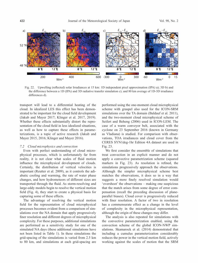
Journal of the Meteorological Society of Japan Vol. 98, No. 2422
transport will lead to a differential heating of the cloud. In idealized LES this effect has been demon-strated to be important for the cloud fi eld development (Jakub and Mayer 2017; Klinger et al. 2017, 2019). Whether these effects substantially distort the repre-sentation of the cloud fi eld in less idealized situations, as well as how to capture these effects in parame-terizations, is a topic of active research (Jakub and Mayer 2015, 2016; Klinger and Mayer 2016).
7.2 Cloud microphysics and convectionEven with perfect understanding of cloud micro-
physical processes, which is unfortunately far from reality, it is not clear what scales of fl uid motion infl uence the microphysical development of clouds. Certainly, the distribution of vertical velocities is important (Reutter et al. 2009), as it controls the adi-abatic cooling and warming, the rate of water phase changes, and how hydrometeors of different sizes are transported through the fl uid. As storm-resolving and large-eddy models begin to resolve the vertical motion fi eld (Fig. 4), they start to create a physical basis for capturing some of these effects.
The advantage of resolving the vertical motion fi eld for the representation of cloud microphysical processes becomes evident from a comparison of sim-ulations over the NA domain that apply progressively fi ner resolution and different degrees of microphysical complexity. For these purposes, additional simulations are performed as a sensitivity study for one of the simulated NA days (these additional simulations have not been listed in Table 1). In these simulations the grid-spacing of the simulations is varied from 2.5 km to 80 km, and simulations at each grid-spacing are
performed using the one-moment cloud microphysical scheme with graupel also used for the ICON-SRM simulations over the TA domain (Baldauf et al. 2011), and the two-moment cloud microphysical scheme of Seifert and Beheng (2006) used in ICON-LEM. The case of a warm conveyor belt, associated with the cyclone on 23 September 2016 (known in Germany as Vladiana) is studied. For comparison with obser-vations, TOA irradiances and cloud cover from the CERES SYN1deg-1hr Edition 4A dataset are used in Fig. 23.
We fi rst consider the ensemble of simulations that treat convection in an explicit manner and do not apply a convective parametrization scheme (squared markers in Fig. 23). As resolution is refi ned, the simulations progressively approach the observations. Although the simpler microphysical scheme best matches the observations, it does so in a way that suggests a more fi nely resolved simulation would ‘overshoot’ the observations – making one suspicious that the match arises from some degree of error com-pensation (recall the preceding discussion of plane-parallel biases). Cloud cover is progressively reduced with fi ner resolution. A factor of two in resolution has a commensurate effect as a change in the level of complexity in the microphysical representation, although the origin of these changes may differ.
The analysis is also repeated for simulations with the convective parameterization enabled, using the convection scheme of the global ICON-NWP sim-ulations. Skamarock et al. (2014) demonstrated that including a cumulus parameterization considerably reduces the power in the vertical motion fi eld, actively working against the scales of motion that the SRM
Fig. 22. Upwelling (refl ected) solar Irradiances at 15 km: 1D independent pixel approximation (IPA) a); 3D b) and the difference between a 1D (IPA) and 3D radiative transfer simulation c); and 80 km average of 1D-3D irradiance differences d).
48 ºN
52 ºN
8 ºE 12 ºE 8 ºE 12 ºE 8 ºE 12 ºE 8 ºE 12 ºE
200 600400 -300 3000 -60 150
a) b) c)
8 ºE 12 ºE 8 ºE 12 ºE 8 ºE 12 ºE 8 ºE 12 ºE
d)
Wm-2 Wm-2 Wm-2
E1D - E3DE1D - E3DE3DE1D

B. STEVENS et al.April 2020 423
is trying to resolve. This might explain why for sim-ulations with parameterized convection an increase in resolution beyond 10 km no longer has an impact and the simulations stall at some distance from the observations. This may also explain the substantially reduced sensitivity to the microphysical representation when convection is parameterized. The impact of the microphysical scheme is much larger for simulations with explicit convection, which is linked to a substan-tial microphysical sensitivity of high-level clouds and cloud ice in the simulations with explicit convection (not shown). By contrast, the sensitivity of low-level clouds and cloud liquid to the microphysical scheme is smaller and less systematic and does not appear to be strongly modulated by the presence or absence of a convection scheme. This may reflect the fact that even at the finest grid spacings of 2.5 km, low-level clouds remain marginally resolved (recall Fig. 21), thereby damping the coupling of the microphysics to the dynamics even in the absence of convective parame-terization.
From this analysis, we hypothesize that a model setup with explicit convection is favorable, as it
allows the differences in the representation of cloud microphysics, as well as its coupling to the dynamics, to be represented more physically. An open question is to what extent the effects of unresolved motions on the microphysical development of clouds can be adequately represented. There are reasons to be opti-mistic that these types of parameterization problems might be more solvable than those posed by more coarsely resolved models with parameterized convec-tion. These prospects depend on the extent to which the effects of the microphysical processes can be observed, using satellites and ground-based networks, on the same scale on which they are simulated, and on the similarity between the unresolved motions and those that begin to become resolved at 2 km and finer.
7.3 Small-scale turbulenceSmall-scale turbulence, particularly in regions of
stratification or near the surface, can have a large influence on matter and energy transports as well as cloud formation. Here mixing on scales of centimeters can become important, and is far from being resolved, even by LES (Ansorge and Mellado 2016; Mellado et al. 2018; van Stratum and Stevens 2018). However, non-turbulent motions, e.g., mesoscale motions and flow circulations are resolved on hecto and kilometer scales, and these can increase shear locally and trigger intermittent turbulence.
Given the still relatively coarse scales, as compared to the scales of nocturnal turbulence near the surface, we investigate the ability of the ICON-LEM – espe-cially as compared to the global models – to simulate the bulk statistics of the small-scale vertical motions. To do so we compare the vertical velocity statistics from eight nights in 2013 (20, 24 – 26 Apr, 2, 5, 11, 28 May) of simulation over JOYCE-CF with wind lidar measurements at the site. Not only does the ICON-LEM capture the variance in the vertical wind in the lower 1.5 km above the site (Fig. 24), but it also represents the intermittent character of the turbulence well. The latter is quantified following Rotta (1956), where the fraction of the night that is turbulent (inter-mittency factor γ) and the number of turbulent events per night (intermittency number n) are described (see Fig. 24b). In calculating these statistics, we distin-guish between non-turbulent and turbulent events, using a threshold of one standard deviation of the total duration of the observed or model-output signals of σw . Each of the signals is normalized by its maximum value. The σw within the nocturnal boundary layer (NBL) was calculated as an average in height up to 1.5 km from the surface, and for each time step.
Fig. 23. TOA shortwave cloud-radiative effect and total cloud cover in ICON-NWP North Atlantic simulations across a range of horizontal resolu-tions, for parameterized or explicit convection, and for two cloud microphysical schemes. Circles denote simulations that include a convective parameterization scheme, squares denote sim-ulations without such a scheme. Filled markers denote simulations with DWD’s operational one- moment cloud microphysical scheme (including graupel), open markers denote simulations with the 2-moment scheme. All values are averaged between 50°W – 10°E and 30 – 70°N, and from 22 Sep 2016 (1200 UTC) to 25 Sep 2016 (2350 UTC). The black cross shows values over the same spatial area and time period according to observations from CERES SYN1deg-1Hr Edition 4A.
SW-C
RE /
Wm
-2
-55
-25
cloud cover / %55 70
CERES

Journal of the Meteorological Society of Japan Vol. 98, No. 2424
The ICON-LEM is, therefore, able to resolve parts of the intermittent character of the NBL turbulence which the coarse simulations cannot capture. Although the horizontal grid-spacing of 156 m is still not suf-ficient to resolve smaller (sub-meso and turbulence) scales of the NBLs, case studies indicate that the model is able to simulate the effects of larger (meso-) scales (e.g., low-level jets) on NBL turbulence vari-ability, and thus capture important preconditioning circulations to which the smaller scales should be responding (Marke et al. 2018). This is encouraging for the hypothesis that some of the smaller scales of motion that are not directly captured by the LEM or SRM, can be more readily parameterized as the condi-tions that cause the motion are resolved.
8. Summary
We report on very large domain storm-resolving (1.25 km to 2.5 km grid mesh) and large-eddy (156 m grid mesh) simulations designed to test the hypothesis that by resolving motions in the atmosphere’s third (vertical) dimension, a much better representation of clouds and precipitation becomes possible. Twenty simulated days were performed and evaluated over Germany, a heavily instrumented region in central Europe, with grid spacings of 156 m over a region with a north-south extent approaching 1000 km. Complementing these simulations are storm-resolving (kilometer) scale simulations spanning the North Atlantic (14 days), the Tropical Atlantic (62 days),
and the Maritime Continent and East Asia (15 days), as well as large-eddy resolving simulations in sub-domains of the Tropical Atlantic, where extensive ground-based and airborne measurement data have been collected. The realism of the simulations and the synoptic conditions in which they are performed allows them to be quantitatively compared to data, and to coarsely resolved simulations that are the state-of-the-art in climate modeling. Further aiding such an evaluation is the ability of the simulations to resolve scales of motion similar to those observed.
In accordance with earlier studies, the energy spectra show that the variance of the vertical velocity has its energy uniformly distributed across all scales larger than a few kilometers. Contributions to the vari-ance only begins to diminish as the scales of three- dimensional turbulence begin to be resolved, at grid spacings on the order of hundreds of meters. Hence, at storm-resolving scales the vertical dimension of the atmospheric motions begins to become resolved. Given the importance of vertical motions for cloud and precipitation development, and thus the exchange of energy in the vertical, this is not a trivial distinc-tion.
In almost every respect, the ability to represent the vertical motion field leads to an improved, and more physical, representation of clouds and precipitation compared to models using parameterizations to represent cloud macrophysics and moist convective processes. In some fields, such as the distribution of condensate (liquid and liquid/ice) water path, or the size distribution and diel evolution of clouds and precipitation, the hectometer scale simulations are difficult to discriminate from the observations. Improvements in precipitation include a better spatial distribution, a more realistic propagation of precip-itating systems, and a greatly improved diel cycle. These improvements include not only the timing and amplitude of the daily maximum in precipitation but also the evolution of precipitation through the night.
A novelty of the present study is its extension to hectometer scales. Here changes in precipitation as the grid is further refined tend to be smaller than differences between simulations with explicit versus parameterized changes. There are quantitative chang-es, a systematic reduction of precipitation, as finer (hectometer) scales are being resolved, and progres-sive improvement in the representation of nocturnal precipitation, as well as a steepening of the frequency distribution of precipitation, indicative of relatively fewer extremes. Despite progressive improvement in precipitation at hectometer scales, our findings give us
Fig. 24. Standard deviation of vertical wind, σw , and intermittent turbulence over eight nights in 2013 for the different simulations and the ob-servations. Here ICON-LEM denotes the 156 m DE configuration. In panel (a) σw is illustrated graphically by the symbols, and the whiskers denote night-to-night variability. In panel (b) the intermittency factor, γ (graphical symbols), and the intermittency number, n (numbers above symbols), are presented for the same platforms (see text for details).
ICON-LEM (156 m)
OBS
ICON-NWP
ECHAM

B. STEVENS et al.April 2020 425
confidence that many biases in the simulation of the hydrological cycle by global climate models would already be addressed by running models at kilometer scales.
Clouds also exhibit systematic improvements as the grid mesh is refined to hectometer scales. Particu-larly over the Tropical Atlantic, simulations on these scales better represent the observed structure of the shallow clouds. Over land as well, the simulations over Germany indicate an improved life cycle and spatial distribution of boundary layer clouds. In storm- resolving simulations (i.e., models with kilometer grid spacings), there is a hint of some of the features, such as a better representation of the diel cycle and a clearer distinction between cumulus and stratiform cloud contributions to trade-wind cloud regimes, that emerge at higher resolution. Simulations in which the grid spacing is progressively increased and in which deep convection is not parameterized, also show a more physical coupling (convergence behavior) between cloud dynamic and microphysical represen-tation. Likewise even for scales of motion that one would not expect to be resolved at hectometer scales, such as those associated with the nocturnal boundary layer, the simulations do a surprisingly good job at capturing the spatiotemporal structure and variability that is observed in the vertical motion field.
Our investigations suggest that the parameterization problems associated with the remaining unresolved degrees of freedom appear to be better constrained, either through a better representation of their drivers or through a greater affinity to data. However, some new problems also emerge at higher resolution, for instance, the need to account in some manner for hori-zontal photon transport.
Many of our findings may not seem surprising, as to hypothesize that a model that begins to resolve the vertical dimension of the atmospheric motion field by using the basic laws of physics, is better at represent-ing clouds and precipitation. Nonetheless, when dis-cussing the advantages of storm resolving simulations, our experience is that many colleagues are quick to point out the remaining deficiencies of such models, to the point where they sometimes even questions whether there is a net benefit from such approaches at all.
Looking forward, as global simulations are now becoming practical at storm-resolving scales, the first climate projections using these types of simulations can be expected to follow in a few years (Stevens et al. 2019b). The first global LES, of a day or two in duration, are being anticipated on a similar time hori-
zon (Satoh et al. 2019). Unless something happens to drastically change the landscape of information tech-nology it seems unlikely however, that long, multi- year, global LES will ever become possible. Hence, the best hope is that global storm-resolving models capture enough of the motion field in the atmosphere’s third dimension, and that the smart application of observations combined with short snapshots from global LES can be combined in ways that usefully constrain important degrees of freedom that are still not adequately captured at kilometer scales. If society hopes to anticipate how warming will change regional climate, particularly possibly large changes that would accompany shifts in circulation systems, then the present study leads us to believe that it will most likely follow from the intensive development and application of storm resolving models to the climate problem, globally.
Acknowledgments
The project HD(CP)2 (High Definition Clouds and Precipitation for advancing Climate Prediction) was funded by the German Federal Ministry of Education and Research within the framework programme “Research for Sustainable Development (FONA)” under the numbers 01LK1501 – 01LK1508A and 01LK1509A. We gratefully acknowledge the com-puting time that was granted by the German Climate Computing Center (DKRZ) and thank its various groups for the support in performing the simulations and in the data handling. Data were provided by Jülich Observatory for Cloud Evolution (JOYCE-CF), a core facility funded by Deutsche Forschungsgemeinschaft via grant DFG LO 901/7-1. We would like to thank Armin Mathes, Paul Dostal and Jochen Elberskirch for the administration of the project and their unwav-ering support. The manuscript also benefited from the insightful input of an editor, Akira Noda, Christoph Schär and an anonymous reviewer. The study was de-signed and executed by the lead authors (BS, CA, AH, RH, CK, DK, HR, WS, and JW), but all authors con-tributed to some element of the study, by contributing to the analysis, the conception of the analysis, or the interpretation of the results. All authors have read the manuscript. Vasileios Barlakas’ present affiliation is at Chalmers University of Technology, Gothenburg, Sweden.

Journal of the Meteorological Society of Japan Vol. 98, No. 2426
Appendix: Tables of integrals
Table A1. Observational data that was used in this study (various figures and bulk quantities in Tables A2–6, including details on the data sets and their sources.
Data Set Products/Variables used and reference as applicableASCAT Twice daily scatterometer winds (over water); Ricciardulli and Wentz (2015)BCO Vertically resolved column observations of thermodynamics and clouds (PW and LWP) at 2 s resolu-
tion; Stevens et al. (2016)CERES TOA and SFC shortwave/longwave irradiances from daily mean at 1°; Wielicki et al. (1996); Loeb
et al. (2018)CiPS Cirrus fraction (5 min at ca. 3.1 km × 6 km, at domain centre); Strandgren et al. (2017a, b)CMORPH Low orbiter satellite microwave observations; Joyce et al. (2004)CMSAF Daily mean TOA irradiances from CMSAF baseline area, MSG disk & arctic (v303), and fractional
cloud cover (MSG3, full disk, v340 and v350) and precipitable water (HTW ATOS v350, global daily-mean data
Ceilometer network Cloud base height (15 min data) from DWD ceilometer network over Germany; PID:de.koeln.rrzk/amd.de.hdfd/igmk.cmnet00.l2.zcb
Weather stations Surface winds at 10 min intervals over Germany from the full domain (196 DWD stations in total)ERA-interim Surface enthalpy fluxes, T2m , V10m , from 0.75° × 0.75° grid; Dee et al. (2011)GPM Precipitation 0.1°, hourly mean; Huffman et al. (2015); Hou et al. (2014)GPCP Daily (1°) gridded precipitation; Hufffman et al. (2001); Adler et al. (2003)HAMP Radar reflectivity 1 s by 30 m; Jacob et al. (2019)HOAPS Latent heat fluxes retrieved from microwave measurementsJOYCE-CF Vertical profiles of thermodynamics, turbulence, winds and clouds (1 s to 1 min); Löhnert et al.
(2015); Cloudnet target classification (http://devcloudnet.fmi.fi/); Illingworth et al. (2007)MAC-LWP Microwave (satellite) retrievals of liquid water path; Elsaesser et al. (2017)MODIS Cloud water path from Aqua and Terra (https://modaps.modaps.eosdis.nasa.gov/services/about/
products/c6/MOD06_L2.html) at 1 km nadir; Nakajima et al. (1990); Platnick et al. (2014)MSG-SEVIRI Liquid and cloud water path (15 min at ca. 3.1 km × 6 km, at domain center); Roebeling et al. (2006);
Schulz et al. (2009)NTAS Buoy T2m , wind speed, precipitationRADOLAN Hourly rain rates derived from combination of rain gauges with radar reflectivities from German
precipitation radar network; Bartels et al. (2004)RAO 2 min profile data similar to JOYCE-CF for the period 2013–2016; https://icdc.cen.uni-hamburg.de/
index.php?id=samd; Cloudnet target classification (http://devcloudnet.fmi.fi/); Illingworth et al. (2007)
TRMM (1°), hourly precipitation rates from an integrated active and passive microwave satellite product; Human et al. (2007)
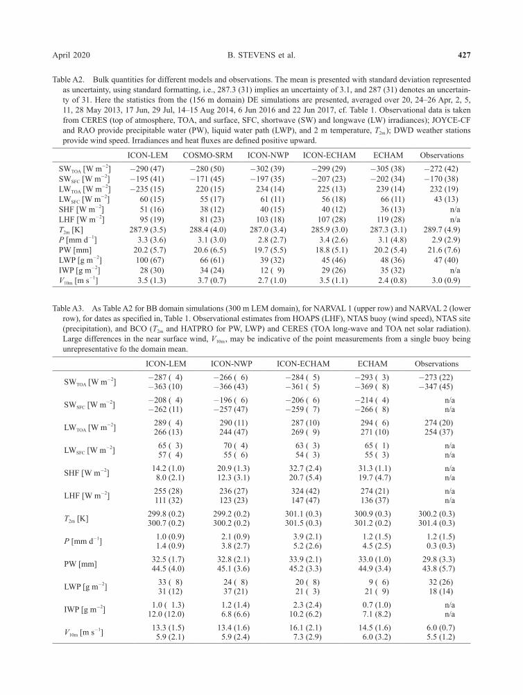
B. STEVENS et al.April 2020 427
Table A2. Bulk quantities for different models and observations. The mean is presented with standard deviation represented as uncertainty, using standard formatting, i.e., 287.3 (31) implies an uncertainty of 3.1, and 287 (31) denotes an uncertain-ty of 31. Here the statistics from the (156 m domain) DE simulations are presented, averaged over 20, 24–26 Apr, 2, 5, 11, 28 May 2013, 17 Jun, 29 Jul, 14–15 Aug 2014, 6 Jun 2016 and 22 Jun 2017, cf. Table 1. Observational data is taken from CERES (top of atmosphere, TOA, and surface, SFC, shortwave (SW) and longwave (LW) irradiances); JOYCE-CF and RAO provide precipitable water (PW), liquid water path (LWP), and 2 m temperature, T2m ); DWD weather stations provide wind speed. Irradiances and heat fluxes are defined positive upward.
ICON-LEM COSMO-SRM ICON-NWP ICON-ECHAM ECHAM ObservationsSWTOA [W m-2]SWSFC [W m-2]LWTOA [W m-2]LWSFC [W m-2]SHF [W m-2]LHF [W m-2]T2m [K]P [mm d-1]PW [mm]LWP [g m-2]IWP [g m-2]V10m [m s-1]
-290 (47)-195 (41)-235 (15)
60 (15)51 (16)95 (19)
287.9 (3.5)3.3 (3.6)
20.2 (5.7)100 (67)28 (30)
3.5 (1.3)
-280 (50)-171 (45)
220 (15)55 (17)38 (12)81 (23)
288.4 (4.0)3.1 (3.0)
20.6 (6.5)66 (61)34 (24)
3.7 (0.7)
-302 (39)-197 (35)
234 (14)61 (11)40 (15)
103 (18)287.0 (3.4)
2.8 (2.7)19.7 (5.5)
39 (32)12 ( 9)
2.7 (1.0)
-299 (29)-207 (23)
225 (13)56 (18)40 (12)
107 (28)285.9 (3.0)
3.4 (2.6)18.8 (5.1)
45 (46)29 (26)
3.5 (1.1)
-305 (38)-202 (34)
239 (14)66 (11)36 (13)
119 (28)287.3 (3.1)
3.1 (4.8)20.2 (5.4)
48 (36)35 (32)
2.4 (0.8)
-272 (42)-170 (38)
232 (19)43 (13)
n/an/a
289.7 (4.9)2.9 (2.9)
21.6 (7.6)47 (40)
n/a3.0 (0.9)
Table A3. As Table A2 for BB domain simulations (300 m LEM domain), for NARVAL 1 (upper row) and NARVAL 2 (lower row), for dates as specified in, Table 1. Observational estimates from HOAPS (LHF), NTAS buoy (wind speed), NTAS site (precipitation), and BCO (T2m and HATPRO for PW, LWP) and CERES (TOA long-wave and TOA net solar radiation). Large differences in the near surface wind, V10m , may be indicative of the point measurements from a single buoy being unrepresentative fo the domain mean.
ICON-LEM ICON-NWP ICON-ECHAM ECHAM Observations
SWTOA [W m-2] -287 ( 4)-363 (10)
-266 ( 6)-366 (43)
-284 ( 5)-361 ( 5)
-293 ( 3)-369 ( 8)
-273 (22)-347 (45)
SWSFC [W m-2] -208 ( 4)-262 (11)
-196 ( 6)-257 (47)
-206 ( 6)-259 ( 7)
-214 ( 4)-266 ( 8)
n/an/a
LWTOA [W m-2] 289 ( 4)266 (13)
290 (11)244 (47)
287 (10)269 ( 9)
294 ( 6)271 (10)
274 (20)254 (37)
LWSFC [W m-2] 65 ( 3)57 ( 4)
70 ( 4)55 ( 6)
63 ( 3)54 ( 3)
65 ( 1)55 ( 3)
n/an/a
SHF [W m-2] 14.2 (1.0)8.0 (2.1)
20.9 (1.3)12.3 (3.1)
32.7 (2.4)20.7 (5.4)
31.3 (1.1)19.7 (4.7)
n/an/a
LHF [W m-2] 255 (28)111 (32)
236 (27)123 (23)
324 (42)147 (47)
274 (21)136 (37)
n/an/a
T2m [K] 299.8 (0.2)300.7 (0.2)
299.2 (0.2)300.2 (0.2)
301.1 (0.3)301.5 (0.3)
300.9 (0.3)301.2 (0.2)
300.2 (0.3)301.4 (0.3)
P [mm d-1] 1.0 (0.9)1.4 (0.9)
2.1 (0.9)3.8 (2.7)
3.9 (2.1)5.2 (2.6)
1.2 (1.5)4.5 (2.5)
1.2 (1.5)0.3 (0.3)
PW [mm] 32.5 (1.7)44.5 (4.0)
32.8 (2.1)45.1 (3.6)
33.9 (2.1)45.2 (3.3)
33.0 (1.0)44.9 (3.4)
29.8 (3.3)43.8 (5.7)
LWP [g m-2] 33 ( 8)31 (12)
24 ( 8)37 (21)
20 ( 8)21 ( 3)
9 ( 6)21 ( 9)
32 (26)18 (14)
IWP [g m-2] 1.0 ( 1.3)12.0 (12.0)
1.2 (1.4)6.8 (6.6)
2.3 (2.4)10.2 (6.2)
0.7 (1.0)7.1 (8.2)
n/an/a
V10m [m s-1] 13.3 (1.5)5.9 (2.1)
13.4 (1.6)5.9 (2.4)
16.1 (2.1)7.3 (2.9)
14.5 (1.6)6.0 (3.2)
6.0 (0.7)5.5 (1.2)

Journal of the Meteorological Society of Japan Vol. 98, No. 2428
Table A4. As Table A2 for TA (2.5 km) domain simulations, for dates as specified in, Table 1. Observed data is taken from TRMM (precipitation), MAC (LWP), ASCAT (wind speed), BCO T2m and BCO HATPRO (LWP, PW) and CERES (TOA long-wave and TOA net solar radiation). SW LWP and PW are calculated for all days in Dec 2013 and Aug 6–31 2016 (no data available for first days of the month). The upper row denotes the values for the NARVAL 1 campaign, the lower row for NARVAL 2.
ICON-SRM ICON-NWP ICON-ECHAM ECHAM Observations
SWTOA [W m-2] -282.5 (4.5)-305.5 (4.4)
-301.5 (5.9)-328.6 (4.3)
-296.5 (5.1)-324.0 (3.9)
-299.5 (6.1)-328.3 (4.0)
-291.0 (43.1)-320.2 (31.6)
SWSFC [W m-2] -190.3 (3.9)-202.2 (4.0)
-209.8 (5.7)-226.8 (4.5)
-205.4 (4.9)-222.1 (3.7)
-202.4 (6.3)-222.0 (3.9)
n/an/a
LWTOA [W m-2] 268.4 (3.0)268.7 (3.0)
264.0 (4.2)265.3 (4.1)
264.2 (3.8)266.2 (3.8)
264.7 (3.4)267.2 (3.9)
257.6 (20.5)261.0 (22.9)
LWSFC [W m-2] 55.6 (1.8)47.2 (1.4)
64.9 (2.0)57.6 (1.8)
55.9 (1.9)49.3 (1.7)
56.1 (2.2)51.0 (1.4)
n/an/a
SHF [W m-2] 25.7 (2.2)27.6 (0.8)
27.2 (2.4)32.6 (0.8)
35.0 (2.9)36.9 (1.5)
23.6 (2.6)25.9 (1.2)
n/an/a
LHF [W m-2] 111 (19)97.6 (6.2)
108 (16)95.8 (5.1)
137 (26)188.8 (7.5)
123 (17)116.0 (5.2)
n/an/a
T2m [K] 298.3 (0.4)299.1 (0.1)
298.0 (0.4)299.2 (0.1)
298.7 (0.2)299.8 (0.1)
298.5 (0.2)299.4 (0.1)
300.1 (0.4)301.7 (0.4)
P [mm d-1] 2.1 (0.5)2.8 (0.4)
2.4 (0.5)2.7 (0.3)
3.5 (0.7)4.2 (0.5)
2.7 (0.6)3.3 (0.4)
2.7 (0.4)3.1 (0.2)
PW [mm] 37.2 (1.5)42.3 (1.4)
36.9 (1.5)41.9 (1.4)
37.3 (1.4)41.9 (1.5)
38.3 (1.4)42.3 (1.4)
33.3 (7.3)40.5 (6.2)
LWP [g m-2] 99 (123)113 ( 7)
43 (10)59 ( 7)
34 ( 7)41 ( 4)
45 (16)53 ( 7)
20 (46)17 (19)
IWP [g m-2] 5.4 (1.7)6.5 (1.2)
8.2 (2.4)8.5 (1.6)
12.6 (4.5)12.7 (2.5)
11.6 (3.9)11.0 (2.8)
n/an/a
V10m [m s-1] 5.0 (0.7)4.6 (0.3)
4.8 (0.7)4.4 (0.3)
5.6 (0.8)5.1 (0.3)
4.8 (0.7)4.4 (0.3)
7.2 (1.0)6.3 (0.4)

B. STEVENS et al.April 2020 429
Table A5. As Table A2 but for NA (2.5 km) domain simulations, as in Table A2, for dates as specified in, Table 1. The values are for 14 selected days of the NAWDEX field campaign (Sep–Oct). Observational data is taken from CERES (short- and long-wave radiation), GPCP (precipitation), CMSAF (PW) and ERA-interim (SHF, LHF, T2m , and V10m ). LWP is a September-October average from MAC.
ICON-SRM ICON-NWP ECHAM ObservationsSWTOA [W m-2]SWSFC [W m-2]LWTOA [W m-2]LWSFC [W m-2]SHF [W m-2]LHF [W m-2]T2m [K]P [mm d-1]PW [mm]LWP [g m-2]IWP [g m-2]V10m [m s-1]
-179 ( 19)-121 ( 13)241.8 ( 3.0)62.6 ( 2.5)29.2 ( 2.3)75.6 ( 8.2)
287.5 ( 0.9)2.49 (0.35)20.0 ( 1.2)
78 ( 8)13.0 ( 1.9)5.8 ( 0.4)
-189 ( 19)-129 ( 14)244.4 ( 2.7)67.9 ( 2.6) 22.7 ( 2.3)76.6 ( 6.8)
287.6 ( 0.9)2.53 (0.34)20.3 ( 1.3)
56 ( 6)14.3 ( 2.2)5.7 ( 0.4)
-176 ( 19)-116 ( 13)240.6 ( 2.9)58.8 ( 2.1)20.1 ( 2.5)77.0 ( 5.8)
287.8 ( 0.9)2.40 (0.35)20.8 ( 1.3)
69 ( 6)31.7 ( 4.6)5.8 ( 0.4)
-182 ( 20)-120 ( 15)240.5 ( 3.0)55.3 ( 2.6)16.5 ( 2.0)74.0 ( 5.4)
288.0 ( 0.9)2.54 (0.56)21.0 ( 1.4)
91 ( 37)n/a
6.1 ( 0.4)
Table A6. As Table A2 for MCEA domain (2.5 km) simulations, for dates as specified in, Table 1. Observational data is taken from CERES ED3 (short- and long-wave radiation), GPM (precipitation), and from ERA-interim (SHF, LHF, T2m , V10m , PW, LWP, and IWP).
ICON-SRM ICON-NWP ECHAM ObservationsSWTOA [W m-2]SWSFC [W m-2]LWTOA [W m-2]LWSFC [W m-2]LHF [W m-2]SHF [W m-2]T2m [K]P [mm d-1]PW [mm]LWP [g m-2]IWP [g m-2]V10m [m s-1]
-302.1 (3.1)-199.7 (3.3)
242.8 (2.5)43.9 (1.2)18.1 (1.0)
105.2 (4.6)299.3 (0.2)
6.7 (0.3)50.0 (0.8)124 ( 8)22 ( 1)3.9 (0.3)
-312.0 (3.7)-210.0 (3.9)
232.0 (2.9)49.0 (1.3)21.3 (1.0)
108.9 (6.1)299.1 (0.2)
6.8 (0.3)50.3 (0.8)
99 ( 6)25 ( 1)
3.8 (0.3 )
-323.9 ( 3.1)-220.9 ( 3.2)
238.8 ( 2.0)47.2 ( 0.8)21.6 ( 1.6)
129.1 (10.1)300.1 ( 0.2)
7.5 ( 0.4) 50.2 ( 0.9)
61 ( 7) 38 ( 2)4.3 ( 0.4)
-307.7 (3.8)-205.0 (4.2)
228.4 (3.3)48.4 (1.3)15.7 (1.0)
118.1 (6.3)299.8 (0.2)
7.8 (0.8)50.1 (0.7)
90 ( 6)44 ( 3)4.0 (0.3)

Journal of the Meteorological Society of Japan Vol. 98, No. 2430
References
Adler, R. F., G. J. Huffman, A. Chang, R. Ferraro, P.-P. Xie, J. Janowiak, B. Rudolf, U. Schneider, S. Curtis, D. Bolvin, A. Gruber, J. Susskind, P. Arkin, and E. Nelkin, 2003: The version-2 Global Precipitation Cli-matology Project (GPCP) monthly precipitation anal-ysis (1979-present). J. Hydrometeor, 4, 1147–1167.
Ansorge, C., and J. P. Mellado, 2016: Analyses of external and global intermittency in the logarithmic layer of Ekman flow. J. Fluid Mech., 805, 611–635.
Arakawa, A., and W. H. Schubert, 1974: Interaction of a cumulus cloud ensemble with the large-scale envrion-ment, Part I. J. Atmos. Sci., 31, 674–701.
Arnold, N. P., and D. A. Randall, 2015: Global-scale con-vective aggregation: Implications for the Madden- Julian oscillation. J. Adv. Model. Earth Syst., 7, 1499– 1518.
Baldauf, M., A. Seifert, J. Förstner, D. Majewski, M. Raschendorfer, and T. Reinhardt, 2011: Operational convective-scale numerical weather prediction with the COSMO model: Description and sensitivities. Mon. Wea. Rev., 139, 3887–3905.
Barker, H. W., and P. Räisänen, 2006: Radiative sensitivities for cloud structural properties that are unresolved by conventional GCMs. Quart. J. Roy. Meteor. Soc., 131, 3103–3122.
Bartels, H., E. Weigl, T. Reich, P. Lang, A. Wagner, O. Kohler, and N. Gerlach, 2004: Projekt RADOLAN - Routineverfahren zur Online-Aneichung der Radar-niederschlagsdaten mit Hilfe von automatischen Bodenniederschlagsstationen (Ombrometer). Techni-cal report, Deutsche Wetterdienst, 111 pp.
Bechtold, P., N. Semane, P. Lopez, J.-P. Chaboureau, A. Beljaars, and N. Bormann, 2014: Representing equi-librium and nonequilibrium convection in large-scale models. J. Atmos. Sci., 71, 734–753.
Beucher, F., J.-P. Lafore, F. Karbou, and R. Roca, 2014: High-resolution prediction of a major convective period over West Africa. Quart. J. Roy. Meteor. Soc., 140, 1409–1425.
Bley, S., H. Deneke, F. Senf, and L. Scheck, 2017: Metrics for the evaluation of warm convective cloud fields in a large-eddy simulation with Meteosat images. Quart. J. Roy. Meteor. Soc., 143, 2050–2060.
Bony, S., B. Stevens, F. Ament, S. Bigorre, P. Chazette, S. Crewell, J. Delanoë, K. Emanuel, D. Farrell, C. Flamant, S. Gross, L. Hirsch, J. Karstensen, B. Mayer, L. Nuijens, J. H. Ruppert, Jr., I. Sandu, P. Siebesma, S. Speich, F. Szczap, J. Totems, R. Vogel, M. Wendisch, and M. Wirth, 2017: EUREC4A: A field campaign to elucidate the couplings between clouds, convection and circulation. Surv. Geophys., 36, 1529–1568.
Bretherton, C. S., M. E. Peters, and L. E. Back, 2004: Rela-tionships between water vapor path and precipitation over the tropical oceans. J. Climate, 17, 1517–1528.
Bryan, G. H., J. C. Wyngaard, and J. M. Fritsch, 2003: Res-olution requirements for the simulation of deep moist convection. Mon. Wea. Rev., 131, 2394–2416.
Cahalan, R. F., W. Ridgway, W. J. Wiscombe, T. L. Bell, and J. B. Snider, 1994: The albedo of fractal stratocumu-lus clouds. J. Atmos. Sci., 51, 2434–2455.
Cesana, G., and D. E. Waliser, 2016: Characterizing and un-derstanding systematic biases in the vertical structure of clouds in CMIP5/CFMIP2 models. Geophys. Res. Lett., 43, 10538–10546.
Covey, C., P. J. Gleckler, C. Doutriaux, D. N. Williams, A. Dai, J. Fasullo, K. Trenberth, and A. Berg, 2016: Metrics for the diurnal cycle of precipitation: Toward routine benchmarks for climate models. J. Climate, 29, 4461–4471.
Dai, A., F. Giorgi, and K. E. Trenberth, 1999: Observed and model-simulated diurnal cycles of precipitation over the contiguous United States. J. Geophys. Res., 104, 6377–6402.
Dee, D. P., S. M. Uppala, A. J. Simmons, P. Berrisford, P. Poli, S. Kobayashi, U. Andrae, M. A. Balmaseda, G. Balsamo, P. Bauer, P. Bechtold, A. C. M. Beljaars, L. van de Berg, J. Bidlot, N. Bormann, C. Delsol, R. Dragani, M. Fuentes, A. J. Geer, L. Haimberger, S. B. Healy, H. Hersbach, E. V. Hólm, L. Isaksen, P. Kåll-berg, M. Köhler, M. Matricardi, A. P. Mcnally, B. M. Monge-Sanz, J.-J. Morcrette, B.-K. Park, C. Peubey, P. de Rosnay, C. Tavolato, J.-N. Thépaut, and F. Vitart, 2011: The ERA-Interim reanalysis: Configuration and performance of the data assimilation system. Quart. J. Roy. Meteor. Soc., 137, 553–597.
Dipankar, A., B. Stevens, R. Heinze, C. Moseley, G. Zängl, M. Giorgetta, and S. Brdar, 2015: Large eddy simula-tion using the general circulation model ICON. J. Adv. Model. Earth Syst., 7, 963–986.
Düben, P., N. Wedi, and S. Saarinen, 2020: Global simula-tions of the atmosphere at 1.45 km grid-spacing with the Integrated Forecast System. J. Meteor. Soc. Japan, 98, accepted.
Elsaesser, G. S., C. W. O’Dell, M. D. Lebsock, R. Bennartz, T. J. Greenwald, and F. J. Wentz, 2017: The Multi-sensor Advanced Climatology of Liquid Water Path (MAC-LWP). J. Climate, 30, 10193–10210.
Eyring, V., S. Bony, G. A. Meehl, C. A. Senior, B. Stevens, R. J. Stouffer, and K. E. Taylor, 2016: Overview of the Coupled Model Intercomparison Project Phase 6 (CMIP6) experimental design and organization. Geosci. Model Dev., 9, 1937–1958.
Fast, J. D., L. K. Berg, L. Alexander, D. Bell, E. D’Ambro, J. Hubbe, C. Kuang, J. Liu, C. Long, A. Matthews, F. Mei, R. Newsom, M. Pekour, T. Pinterich, B. Schmid, S. Schobesberger, J. Shilling, J. N. Smith, S. Springston, K. Suski, J. A. Thornton, J. Tomlinson, J. Wang, H. Xiao, and A. Zelenyuk, 2019: Overview of the HI-SCALE field campaign: A new perspective on shallow convective clouds. Bull. Amer. Meteor.
B. STEVENS et al.April 2020 431
Soc., 100, 821–840.Gates, W. L., 1992: AMIP: The Atmospheric Model Inter-
comparison Project. Bull. Amer. Meteor. Soc., 73, 1962–1970.
Giorgetta, M. A., R. Brokopf, T. Crueger, M. Esch, S. Fiedler, J. Helmert, C. Hohenegger, L. Kornblueh, M. Köhler, E. Manzini, T. Mauritsen, C. Nam, T. Radd-atz, S. Rast, D. Reinert, M. Sakradzija, H. Schmidt, R. Schneck, R. Schnur, L. Silvers, H. Wan, G. Zängl, and B. Stevens, 2018: ICON-A, the atmosphere com-ponent of the ICON earth system model: I. Model de-scription. J. Adv. Model. Earth Syst., 10, 1613–1637.
Grandpeix, J.-Y., and J.-P. Lafore, 2010: A density current parameterization coupled with Emanuel’s convection scheme. Part I: The models. J. Atmos. Sci., 67, 881– 897.
Guichard, F., and F. Couvreux, 2017: A short review of numerical cloud-resolving models. Tellus A, 69, 1373578, doi:10.1080/16000870.2017.1373578.
Harshvardhan, and R. C. Espinoza, Jr., 1995: Simple param-eterizations of the radiative properties of cloud layers: a review. Atmos. Res., 35, 113–125.
Heinze, R., A. Dipankar, C. C. Henken, C. Moseley, O. Sourdeval, S. Trömel, X. Xie, P. Adamidis, F. Ament, H. Baars, C. Barthlott, A. Behrendt, U. Blahak, S. Bley, S. Brdar, M. Brueck, S. Crewell, H. Deneke, P. Di Girolamo, R. Evaristo, J. Fischer, C. Frank, P. Frie-derichs, T. Göcke, K. Gorges, L. Hande, M. Hanke, A. Hansen, H.-C. Hege, C. Hoose, T. Jahns, N. Kalthoff, D. Klocke, S. Kneifel, P. Knippertz, A. Kuhn, T. van Laar, A. Macke, V. Maurer, B. Mayer, C. I. Meyer, S. K. Muppa, R. A. J. Neggers, E. Orlandi, F. Pantillon, B. Pospichal, N. Röber, L. Scheck, A. Seifert, P. Seifert, F. Senf, P. Siligam, C. Simmer, S. Steinke, B. Stevens, K. Wapler, M. Weniger, V. Wulfmeyer, G. Zängl, D. Zhang, and J. Quaas, 2017: Large-eddy simulations over Germany using ICON: A comprehensive evalua-tion. Quart. J. Roy. Meteor. Soc., 143, 69–100.
Hentgen, L., N. Ban, N. Kröner, D. Leutwyler, and C. Schär, 2019: Clouds in convection-resolving climate simula-tions over Europe. J. Geophys. Res., 124, 3849–3870.
Hirahara, Y., J. Ishida, and T. Ishimizu, 2011: Trial operation of the Local Forecast Model at JMA. CAS/JSC WGNE Res. Act. Atmos. Oceanic Modell., 41, 5.11–5.12.
Hohenegger, C., P. Brockhaus, and C. Schär, 2008: Towards climate simulations at cloud-resolving scales. Meteor. Z., 17, 383–394.
Hohenegger, C., L. Kornblueh, D. Klocke, T. Becker, G. Cioni, J. F. Engels, U. Schulzweida, and B. Stevens, 2020: Climate statistics in gobal simulations of the at-mosphere, from 80 to 2.5 km grid spacing. J. Meteor. Soc. Japan, 98, 73–91.
Holloway, C. E., and J. D. Neelin, 2009: Moisture vertical structure, column water vapor, and tropical deep con-vection. J. Atmos. Sci., 66, 1665–1683.
Holloway, C. E., S. J. Woolnough, and G. M. S. Lister,
2012: Precipitation distributions for explicit versus parametrized convection in a large-domain high- resolution tropical case study. Quart. J. Roy. Meteor. Soc., 138, 1692–1708.
Hou, A. Y., R. K. Kakar, S. Neeck, A. A. Azarbarzin, C. D. Kummerow, M. Kojima, R. Oki, K. Nakamura, and T. Iguchi, 2014: The Global Precipitation Measurement mission. Bull. Amer. Meteor. Soc., 95, 701–722.
Hourdin, F., J.-Y. Grandpeix, C. Rio, S. Bony, A. Jam, F. Cheruy, N. Rochetin, L. Fairhead, A. Idelkadi, I. Musat, J.-L. Dufresne, A. Lahellec, M.-P. Lefebvre, and R. Roehrig, 2013: LMDZ5B: The atmospheric component of the IPSL climate model with revisited parameterizations for clouds and convection. Climate Dyn., 40, 2193–2222.
Huffman, G. J., R. F. Adler, M. M. Morrissey, D. T. Bolvin, S. Curtis, R. Joyce, B. McGavock, and J. Susskind, 2001: Global precipitation at one-degree daily resolu-tion from multisatellite observations. J. Hydrometeor, 2, 36–50.
Huffman, G. J., D. T. Bolvin, E. J. Nelkin, D. B. Wolff, R. F. Adler, G. Gu, Y. Hong, K. P. Bowman, and E. F. Stocker, 2007: The TRMM Multisatellite Precipitation Analysis (TMPA): Quasi-global, multiyear, combined- sensor precipitation estimates at fine scales. J. Hydro-meteor, 8, 38–55.
Huffman, G. J., D. T. Bolvin, D. Braithwaite, K. Hsu, R. Joyce, C. Kidd, E. J. Nelkin, and P. Xie, 2015: NASA Global Precipitation Measurement (GPM) Integrated Multi-Satellite Retrievals for GPM (IMERG). Algo-rithm Theoretical Basis Document (ATBD) Version 4.5. NASA: Greenbelt, MD, USA, 26 pp.
Illingworth, A. J., R. J. Hogan, E. J. O’Connor, D. Bouniol, M. E. Brooks, J. Delanoé, D. P. Donovan, J. D. East-ment, N. Gaussiat, J. W. F. Goddard, M. Haeffelin, H. Klein Baltink, O. A. Krasnov, J. Pelon, J.-M. Piriou, A. Protat, H. W. J. Russchenberg, A. Seifert, A. M. Tompkins, G.-J. van Zadelhoff, F. Vinit, U. Willén, D. R. Wilson, and C. L. Wrench, 2007: Cloudnet: Continuous evaluation of cloud profiles in seven oper-ational models using ground-based observations. Bull. Amer. Meteor. Soc., 88, 883–898.
Jacob, M., F. Ament, M. Gutleben, H. Konow, M. Mech, M. Wirth, and S. Crewell, 2019: Investigating the liquid water path over the tropical Atlantic with synergistic airborne measurements. Atmos. Meas. Tech., 12, 3237–3254.
Jakob, C., 2010: Accelerating progress in global atmospheric model development through improved parameteriza-tions. Bull. Amer. Meteor. Soc., 91, 869–876.
Jakub, F., and B. Mayer, 2015: A three-dimensional parallel radiative transfer model for atmospheric heating rates for use in cloud resolving models—The TenStream solver. J. Quant. Spectrosc. Radiat. Transfer, 163, 63– 71.
Jakub, F., and B. Mayer, 2016: 3-D radiative transfer in

Journal of the Meteorological Society of Japan Vol. 98, No. 2432
large-eddy simulations – experiences coupling the TenStream solver to the UCLA-LES. Geosci. Model Dev., 9, 1413–1422.
Jakub, F., and B. Mayer, 2017: The role of 1-D and 3-D ra-diative heating in the organization of shallow cumulus convection and the formation of cloud streets. Atmos. Chem. Phys., 17, 13317–13327.
Jeevanjee, N., 2017: Vertical velocity in the gray zone. J. Adv. Model. Earth Syst., 9, 2304–2316.
Joyce, R. J., J. E. Janowiak, P. A. ARKIN, and P. Xie, 2004: CMORPH: A method that produces global precipita-tion estimates from passive microwave and infrared data at high spatial and temporal resolution. J. Hydro-meteor, 5, 487–503.
Kendon, E. J., N. Ban, N. M. Roberts, H. J. Fowler, M. J. Roberts, S. C. Chan, J. P. Evans, G. Fosser, and J. M. Wilkinson, 2017: Do convection-permitting regional climate models improve projections of future precipi-tation change? Bull. Amer. Meteor. Soc., 98, 79–93.
Kendon, E. J., R. A. Stratton, S. Tucker, J. H. Marsham, S. Berthou, D. P. Rowell, and C. A. Senior, 2019: En-hanced future changes in wet and dry extremes over Africa at convection-permitting scale. Nat. Commun., 10, 1794, doi:10.1038/s41467-019-09776-9.
Khairoutdinov, M., D. Randall, and C. DeMott, 2005: Simu-lations of the atmospheric general circulation using a cloud-resolving model as a superparameterization of physical processes. J. Atmos. Sci., 62, 2136–2154.
Klinger, C., and B. Mayer, 2016: The Neighboring Column Approximation (NCA) – A fast approach for the calculation of 3D thermal heating rates in cloud re-solving models. J. Quant. Spectrosc. Radiat. Transfer, 168, 17–28.
Klinger, C., B. Mayer, F. Jakub, T. Zinner, S.-B. Park, and P. Gentine, 2017: Effects of 3-D thermal radiation on the development of a shallow cumulus cloud field. Atmos. Chem. Phys., 17, 5477–5500.
Klinger, C., G. Feingold, and T. Yamaguchi, 2019: Cloud droplet growth in shallow cumulus clouds considering 1-D and 3-D thermal radiative effects. Atmos. Chem. Phys., 19, 6295–6313.
Klocke, D., M. Brueck, C. Hohenegger, and B. Stevens, 2017: Rediscovery of the doldrums in storm-resolving simulations over the tropical Atlantic. Nat. Geosci., 10, 891–896.
Knutti, R., and J. Sedláček, 2012: Robustness and uncer-tainties in the new CMIP5 climate model projections. Nat. Climate Change, 3, 369–373.
Koshyk, J. N., and K. Hamilton, 2001: The horizontal kinet-ic energy spectrum and spectral budget simulated by a high-resolution troposphere-stratosphere-mesosphere GCM. J. Atmos. Sci., 58, 329–348.
Kotthaus, S., E. O’Connor, C. Münkel, C. Charlton-Perez, M. Haeffelin, A. M. Gabey, and C. S. B. Grimmond, 2016: Recommendations for processing atmospheric attenuated backscatter profiles from Vaisala CL31
ceilometers. Atmos. Meas. Tech., 9, 3769–3791.Kousky, V. E., 1980: Diurnal rainfall variation in northeast
Brazil. Mon. Wea. Rev., 108, 488–498.Lammert, A., A. Hansen, F. Ament, S. Crewell, G. Dick, V.
Grützun, H. Klein-Baltink, V. Lehmann, A. Macke, B. Pospichal, W. Schubotz, P. Seifert, E. Stamnas, and B. Stevens, 2019: A Standardized Atmospheric Measurement Data archive for distributed cloud and precipitation process-oriented observations in central Europe. Bull. Amer. Meteor. Soc., 100, 1299–1314.
Langhans, W., J. Schmidli, and C. Schär, 2012: Bulk convergence of cloud-resolving simulations of moist convection over complex terrain. J. Atmos. Sci., 69, 2207–2228.
Lean, H. W., P. A. Clark, M. Dixon, N. M. Roberts, A. Fitch, R. Forbes, and C. Halliwell, 2008: Characteristics of high-resolution versions of the Met Office Unified Model for forecasting convection over the United Kingdom. Mon. Wea. Rev., 136, 3408–3424.
Leutwyler, D., D. Lüthi, N. Ban, O. Fuhrer, and C. Schär, 2017: Evaluation of the convection-resolving climate modeling approach on continental scales. J. Geophys. Res., 122, 5237–5258.
Loeb, N. G., D. R. Doelling, H. Wang, W. Su, C. Nguyen, J. G. Corbett, L. Liang, C. Mitrescu, F. G. Rose, and S. Kato, 2018: Clouds and the Earth’s Radiant Energy System (CERES) Energy Balanced and Filled (EBAF) top-of-atmosphere (TOA) Edition-4.0 data product. J. Climate, 31, 895–918.
Löhnert, U., J. H. Schween, C. Acquistapace, K. Ebell, M. Maahn, M. Barrera-Verdejo, A. Hirsikko, B. Bohn, A. Knaps, E. O’Connor, C. Simmer, A. Wahner, and S. Crewell, 2015: JOYCE: Jülich Observatory for Cloud Evolution. Bull. Amer. Meteor. Soc., 96, 1157–1174.
Macke, A., P. Seifert, H. Baars, C. Barthlott, C. Beekmans, A. Behrendt, B. Bohn, M. Brueck, J. Bühl, S. Crewell, T. Damian, H. Deneke, S. Düsing, A. Foth, P. Di Girola-mo, E. Hammann, R. Heinze, A. Hirsikko, J. Kalisch, N. Kalthoff, S. Kinne, M. Kohler, U. Löhnert, B. Lakshmi Madhavan, V. Maurer, S. K. Muppa, J. Schween, I. Serikov, H. Siebert, C. Simmer, F. Späth, S. Steinke, K. Träumner, S. Trömel, B. Wehner, A. Wieser, V. Wulfmeyer, and X. Xie, 2017: The HD(CP)2 Observational Prototype Experiment (HOPE) – an overview. Atmos. Chem. Phys., 17, 4887–4914.
Mapes, B. E., E. S. Chung, W. M. Hannah, H. Masunaga, A. J. Wimmers, and C. S. Velden, 2018: The meandering margin of the meteorological moist tropics. Geophys. Res. Lett., 45, 1177–1184.
Marke, T., S. Crewell, V. Schemann, J. H. Schween, and M. Tuononen, 2018: Long-term observations and high- resolution modeling of midlatitude nocturnal boundary layer processes connected to low-level jets. J. Appl. Meteor. Climatol., 57, 1155–1170.
Marsham, J. H., N. S. Dixon, L. Garcia-Carreras, G. M. S. Lister, D. J. Parker, P. Knippertz, and C. E. Birch,

B. STEVENS et al.April 2020 433
2013: The role of moist convection in the West Afri-can monsoon system: Insights from continental-scale convection-permitting simulations. Geophys. Res. Lett., 40, 1843–1849.
Maurer, V., N. Kalthoff, and L. Gantner, 2015: Predictability of convective precipitation for West Africa: Does the land surface influence ensemble variability as much as the atmosphere? Atmos. Res., 157, 91–107.
Mayer, B., 2009: Radiative transfer in the cloudy atmo-sphere. Eur. Phys. J. Conf., 1, 75–99.
Mellado, J. P., C. S. Bretherton, B. Stevens, and M. C. Wyant, 2018: DNS and LES for simulating stratocu-mulus: Better together. J. Adv. Model. Earth Syst., 10, 1421–1438.
Miura, H., M. Satoh, T. Nasuno, A. T. Noda, and K. Oouchi, 2007: A Madden-Julian Oscillation event realistically simulated by a global cloud-resolving model. Science, 318, 1763–1765.
Miyamoto, Y., Y. Kajikawa, R. Yoshida, T. Yamaura, H. Yashiro, and H. Tomita, 2013: Deep moist atmospher-ic convection in a subkilometer global simulation. Geophys. Res. Lett., 40, 4922–4926.
Moeng, C.-H., 1986: Large-eddy simulation of a stratus- topped boundary layer. Part I: Structure and budgets. J. Atmos. Sci., 43, 2886–2900.
Nakajima, T., and M. D. King, 1990: Determination of the optical thickness and effective particle radius of clouds from reflected solar radiation measurements. Part I: Theory. J. Atmos. Sci., 47, 1878–1893.
Nam, C., S. Bony, J.-L. Dufresne, and H. Chepfer, 2012: The ‘too few, too bright’ tropical low-cloud problem in CMIP5 models. Geophys. Res. Lett., 39, L21801, doi:10.1029/2012GL053421.
Nastrom, G. D., K. S. Gage, and W. H. Jasperson, 1984: Kinetic energy spectrum of large and mesoscale atmo-spheric processes. Nature, 310, 36–38.
Nuijens, L., I. Serikov, L. Hirsch, K. Lonitz, and B. Stevens, 2014: The distribution and variability of low-level cloud in the North Atlantic trades. Quart. J. Roy. Meteor. Soc., 140, 2364–2374.
Palmer, T., and B. Stevens, 2019: The scientific challenge of understanding and estimating climate change. Proc. Natl. Acad. Sci. U. S. A., 116, 24390–24395.
Panosetti, D., L. Schlemmer, and C. Schär, 2019: Bulk and structural convergence at convection-resolving scales in real-case simulations of summertime moist con-vection over land. Quart. J. Roy. Meteor. Soc., 145, 1427–1443.
Parishani, H., M. S. Pritchard, C. S. Bretherton, C. R. Terai, M. C. Wyant, M. Khairoutdinov, and B. Singh, 2018: Insensitivity of the cloud response to surface warming under radical changes to boundary layer turbulence and cloud microphysics: Results from the ultraparam-eterized CAM. J. Adv. Model. Earth Syst., 10, 3139– 3158.
Pauluis, O., and S. Garner, 2006: Sensitivity of radiative–
convective equilibrium simulations to horizontal resolution. J. Atmos. Sci, 63, 1910–1923.
Pearson, K. J., G. M. S. Lister, C. E. Birch, R. P. Allan, R. J. Hogan, and S. J. Woolnough, 2014: Modelling the diurnal cycle of tropical convection across the ‘grey zone’. Quart. J. Roy. Meteor. Soc., 140, 491–499.
Pedgley, D. E., 1969: Diurnal variation of the incidence of monsoon rainfall over the Sudan (Part I). Meteor. Mag., 98, 97–107.
Petch, J. C., A. R. Brown, and M. E. B. Gray, 2002: The impact of horizontal resolution on the simulations of convective development over land. Quart. J. Roy. Meteor. Soc., 128, 2031–2044.
Peters, K., C. Hohenegger, and D. Klocke, 2019: Different representation of mesoscale convective systems in convection-permitting and convection-parameterizing NWP models and its implications for large-scale forecast evolution. Atmosphere, 10, 503, doi:10.3390/atmos10090503.
Peters, O., and J. D. Neelin, 2006: Critical phenomena in atmospheric precipitation. Nat. Phys., 2, 393–396.
Platnick, S., M. D. King, K. G. Meyer, G. Wind, N. Ama-rasinghe, B. Marchant, G. T. Arnold, Z. Zhang, P. A. Hubanks, B. Ridgway, and J. Riedi, 2014: MODIS Cloud Optical Properties: User Guide for the Collec-tion 6 Level-2 MOD06/MYD06 Product and Associ-ated Level-3 Datasets, Version 0.9. Technical report, NASA.
Prein, A. F., W. Langhans, G. Fosser, A. Ferrone, N. Ban, K. Goergen, M. Keller, M. Tölle, O. Gutjahr, F. Feser, E. Brisson, S. Kollet, J. Schmidli, N. P. M. van Lipzig, and R. Leung, 2015: A review on regional convec-tion-permitting climate modeling: Demonstrations, prospects, and challenges. Rev. Geophys., 53, 323– 361.
Rasp, S., T. Selz, and G. C. Craig, 2018: Variability and clustering of midlatitude summertime convection: Testing the Craig and Cohen theory in a convection- permitting ensemble with stochastic boundary layer perturbations. J. Atmos. Sci., 75, 691–705.
Reutter, P., H. Su, J. Trentmann, M. Simmel, D. Rose, S. S. Gunthe, H. Wernli, M. O. Andreae, and U. Pöeschl, 2009: Aerosol- and updraft-limited regimes of cloud droplet formation: influence of particle number, size and hygroscopicity on the activation of cloud conden-sation nuclei (CCN). Atmos. Chem. Phys., 9, 7067– 7080.
Ricciardulli, L., and F. J. Wentz, 2015: A scatterometer geophysical model function for climate-quality winds: QuikSCAT Ku-2011. J. Atmos. Oceanic Technol., 32, 1829–1846.
Rieck, M., L. Nuijens, and B. Stevens, 2012: Marine boundary layer cloud feedbacks in a constant relative humidity atmosphere. J. Atmos. Sci., 69, 2538–2550.
Roebeling, R. A., A. J. Feijt, and P. Stammes, 2006: Cloud property retrievals for climate monitoring: Implica-

Journal of the Meteorological Society of Japan Vol. 98, No. 2434
tions of differences between Spinning Enhanced Vis-ible and Infrared Imager (SEVIRI) on METEOSAT-8 and Advanced Very High Resolution Radiometer (AVHRR) on NOAA-17. J. Geophys. Res., 111, D20210, doi:10.1029/2005JD006990.
Rotta, J., 1956: Experimenteller Beitrag zur Entstehung tur-bulenter Strömung im Rohr. Ing.-Arch., 24, 258–281.
Sato, T., H. Miura, M. Satoh, Y. N. Takayabu, and Y. Wang, 2009: Diurnal cycle of precipitation in the tropics sim-ulated in a global cloud-resolving model. J. Climate, 22, 4809–4826.
Satoh, M., H. Tomita, H. Yashiro, Y. Kajikawa, Y. Miyamoto, T. Yamaura, T. Miyakawa, M. Nakano, C. Kodama, A. T. Noda, T. Nasuno, Y. Yamada, and Y. Fukutomi, 2017: Outcomes and challenges of global high-reso-lution non-hydrostatic atmospheric simulations using the K computer. Prog. Earth Planet. Sci., 4, 13, doi: 10.1186/s40645-017-0127-8.
Satoh, M., B. Stevens, F. Judt, M. Khairoutdinov, S.-J. Lin, W. M. Putman, and P. Düben, 2019: Global cloud- resolving models. Curr. Climate Change Rep., 5, 172– 184.
Schäfler, A., G. Craig, H. Wernli, P. Arbogast, J. D. Doyle, R. McTaggart-Cowan, J. Methven, G. Rivière, F. Ament, M. Boettcher, M. Bramberger, Q. Cazenave, R. Cotton, S. Crewell, J. Delanoë, A. Dörnbrack, A. Ehrlich, F. Ewald, A. Fix, C. M. Grams, S. L. Gray, H. Grob, S. Groß, M. Hagen, B. Harvey, L. Hirsch, M. Jacob, T. Kölling, H. Konow, C. Lemmerz, O. Lux, L. Magnusson, B. Mayer, M. Mech, R. Moore, J. Pelon, J. Quinting, S. Rahm, M. Rapp, M. Rautenhaus, O. Reitebuch, C. A. Reynolds, H. Sodemann, T. Spengler, G. Vaughan, M. Wendisch, M. Wirth, B. Witschas, K. Wolf, and T. Zinner, 2018: The North Atlantic Wave-guide and Downstream Impact Experiment. Bull. Amer. Meteor. Soc., 99, 1607–1637.
Scheck, L., P. Frèrebeau, R. Buras-Schnell, and B. Mayer, 2016: A fast radiative transfer method for the simula-tion of visible satellite imagery. J. Quant. Spectrosc. Radiat. Transfer, 175, 54–67.
Scheck, L., M. Weissmann, and B. Mayer, 2018: Efficient methods to account for cloud-top inclination and cloud overlap in synthetic visible satellite images. J. Atmos. Oceanic Technol., 35, 665–685.
Schulz, J., P. Albert, H. D. Behr, D. Caprion, H. Deneke, S. Dewitte, B. Dürr, P. Fuchs, A. Gratzki, P. Hechler, R. Hollmann, S. Johnston, K.-G. Karlsson, T. Manninen, R. Müeller, M. Reuter, A. Riihelä, R. Roebeling, N. Selbach, A. Tetzlaff, W. Thomas, M. Werscheck, E. Wolters, and A. Zelenka, 2009: Operational climate monitoring from space: The EUMETSAT Satellite Application Facility on Climate Monitoring (CM-SAF). Atmos. Chem. Phys., 9, 1687–1709.
Seifert, A., and K. D. Beheng, 2006: A two-moment cloud microphysics parameterization for mixed-phase clouds. Part 2: Maritime vs. continental deep convective
storms. Meteorol. Atmos. Phys., 92, 67–82.Seifert, A., T. Heus, R. Pincus, and B. Stevens, 2015: Large-
eddy simulation of the transient and near-equilibrium behavior of precipitating shallow convection. J. Adv. Model. Earth Syst., 7, 1918–1937.
Siebesma, A. P., C. S. Bretherton, A. Brown, A. Chlond, J. Cuxart, P. G. Duynkerke, H. Jiang, M. Khairoutdinov, D. Lewellen, C.-H. Moeng, E. Sanchez, B. Stevens, and D. E. Stevens, 2003: A large eddy simulation in-tercomparison study of shallow cumulus convection. J. Atmos. Sci., 60, 1201–1219.
Siongco, A. C., C. Hohenegger, and B. Stevens, 2014: The Atlantic ITCZ bias in CMIP5 models. Climate Dyn., 45, 1169–1180.
Skamarock, W. C., S.-H. Park, J. B. Klemp, and C. Snyder, 2014: Atmospheric Kinetic energy spectra from global high-resolution nonhydrostatic simulations. J. Atmos. Sci., 71, 4369–4381.
Sommeria, G., and J. W. Deardorff, 1977: Subgrid-scale condensation in models of nonprecipitating clouds. J. Atmos. Sci., 34, 344–355.
Sourdeval, O., L. C.-Labonnote, A. J. Baran, J. Mülmen-städt, and G. Brogniez, 2016: A methodology for simultaneous retrieval of ice and liquid water cloud properties. Part 2: Near-global retrievals and evalua-tion against A-Train products. Quart. J. Roy. Meteor. Soc., 142, 3063–3081.
Stephens, G. L., 1978: Radiation profiles in extended water clouds. II: Parameterization Schemes. J. Atmos. Sci., 35, 2123–2132.
Stevens, B., and D. H. Lenschow, 2001: Observations, experiments, and large eddy Simulation. Bull. Amer. Meteor. Soc., 82, 283–294.
Stevens, B., M. Giorgetta, M. Esch, T. Mauritsen, T. Crueger, S. Rast, M. Salzmann, H. Schmidt, J. Bader, K. Block, R. Brokopf, I. Fast, S. Kinne, L. Kornblueh, U. Lohmann, R. Pincus, T. Reichler, and E. Roeckner, 2013: Atmospheric component of the MPI-M Earth System Model: ECHAM6. J. Adv. Model. Earth Syst., 5, 146–172.
Stevens, B., D. Farrell, L. Hirsch, F. Jansen, L. Nuijens, I. Serikov, B. Brügmann, M. Forde, H. Linne, K. Lonitz, and J. M. Prospero, 2016: The Barbados Cloud Ob-servatory: Anchoring investigations of clouds and cir-culation on the edge of the ITCZ. Bull. Amer. Meteor. Soc., 97, 787–801.
Stevens, B., F. Ament, S. Bony, S. Crewell, F. Ewald, S. Gross, A. Hansen, L. Hirsch, M. Jacob, T. Kölling, H. Konow, B. Mayer, M. Wendisch, M. Wirth, K. Wolf, S. Bakan, M. Bauer-Pfundstein, M. Brueck, J. Delanoë, A. Ehrlich, D. Farrell, M. Forde, F. Gödde, H. Grob, M. Hagen, E. Jäkel, F. Jansen, C. Klepp, M. Klinge-biel, M. Mech, G. Peters, M. Rapp, A. A. Wing, and T. Zinner, 2019a: A high-altitude long-range aircraft configured as a cloud observatory: The NARVAL ex-peditions. Bull. Amer. Meteor. Soc., 100, 1061–1077.
B. STEVENS et al.April 2020 435
Stevens, B., M. Satoh, L. Auger, J. Biercamp, C. S. Breth-erton, X. Chen, P. Düben, F. Judt, M. Khairoutdinov, D. Klocke, C. Kodama, L. Kornblueh, S.-J. Lin, P. Neumann, W. M. Putman, N. Röber, R. Shibuya, B. Vanniere, P. L. Vidale, N. Wedi, and L. Zhou, 2019b: DYAMOND: The DYnamics of the Atmospheric general circulation Modeled On Non-hydrostatic Domains. Prog. Earth Planet. Sci., 6, 61, doi:10.1186/s40645-019-0304-z.
Stietencron, B., 1992: Ein Tag im Garten. Engel, 16 pp.Strandgren, J., L. Bugliaro, F. Sehnke, and L. Schröder,
2017a: Cirrus cloud retrieval with MSG/SEVIRI using artificial neural networks. Atmos. Meas. Tech., 10, 3547–3573.
Strandgren, J., J. Fricker, and L. Bugliaro, 2017b: Character-isation of the artificial neural network CiPS for cirrus cloud remote sensing with MSG/SEVIRI. Atmos. Meas. Tech., 10, 4317–4339.
Takayabu, Y. N., and M. Kimoto, 2008: Diurnal march of rainfall simulated in a T106 AGCM and dependence on cumulus schemes. J. Meteor. Soc. Japan, 86A, 163–173.
Terasaki, K., H. L. Tanaka, and M. Satoh, 2009: Characteris-tics of the kinetic energy spectrum of NICAM model atmosphere. SOLA, 5, 180–183.
Tomita, H., H. Miura, S. Iga, T. Nasuno, and M. Satoh, 2005: A global cloud-resolving simulation: Prelimi-nary results from an aqua planet experiment. Geophys. Res. Lett., 32, L08805, doi:10.1029/2005GL022459.
van Stratum, B. J. H., and B. Stevens, 2018: The impact of vertical mixing biases in large-eddy simulation on nocturnal low clouds. J. Adv. Model. Earth Syst., 10, 1290–1303.
Vial, J., R. Vogel, S. Bony, B. Stevens, D. M. Winker, X.
Cai, C. Hohenegger, A. K. Naumann, and H. Brogniez, 2019: A new look at the daily cycle of trade wind cumuli. J. Adv. Model. Earth Syst., 11, 3148–3166.
Weber, N. J., and C. F. Mass, 2019: Subseasonal weather prediction in a global convection-permitting model. Bull. Amer. Meteor. Soc., 100, 1079–1089.
Weisman, M. L., W. C. Skamarock, and J. B. Klemp, 1997: The resolution dependence of explicitly modeled convective systems. Mon. Wea. Rev., 125, 527–548.
Wiegner, M., F. Madonna, I. Binietoglou, R. Forkel, J. Gasteiger, A. Geiß, G. Pappalardo, K. Schäfer, and W. Thomas, 2014: What is the benefit of ceilometers for aerosol remote sensing? An answer from EARLINET. Atmos. Meas. Tech., 7, 1979–1997.
Wielicki, B. A., B. R. Barkstrom, E. F. Harrison, R. B. Lee III, G. Louis Smith, and J. E. Cooper, 1996: Clouds and the Earth’s Radiant Energy System (CERES): An earth observing system experiment. Bull. Amer. Meteor. Soc., 77, 853–868.
Williams, K. D., A. Bodas-Salcedo, M. Déqué, S. Fermepin, B. Medeiros, M. Watanabe, C. Jakob, S. A. Klein, C. A. Senior, and D. L. Williamson, 2013: The Transpose- AMIP II Experiment and its application to the under-standing of southern ocean cloud biases in climate models. J. Climate, 26, 3258–3274.
Zängl, G., D. Reinert, P. Rípodas, and M. Baldauf, 2015: The ICON (ICOsahedral Non-hydrostatic) modelling framework of DWD and MPI-M: Description of the non-hydrostatic dynamical core. Quart. J. Roy. Meteor. Soc., 141, 563–579.
Zhang, G., K. H. Cook, and E. K. Vizy, 2016: The diurnal cycle of warm season rainfall over West Africa. Part II: Convection-permitting simulations. J. Climate, 29, 8439–8454.