On the Land–Ocean Contrast of Tropical Convection and Microphysics StatisticsDerived from TRMM Satellite Signals and Global Storm-Resolving Models

TOSHI MATSUI,1,# JIUN-DAR CHERN,1,# WEI-KUO TAO,1 STEPHEN LANG,1,@

MASAKI SATOH,& TEMPEI HASHINO,** AND TAKUJI KUBOTA11

1Mesoscale Atmospheric Processes Laboratory, NASA Goddard Space Flight Center, Greenbelt, Maryland#Earth System Science Interdisciplinary Center, University of Maryland, College Park, College Park, Maryland

@ Science Systems and Applications, Inc., Lanham, Maryland&Atmosphere and Ocean Research Institute, University of Tokyo, Tokyo, Japan

** Research Institute for Applied Mechanics, Kyushu University, Fukuoka, Japan11Earth Observing Research Center, Japan Aerospace Exploration Agency, Tsukuba, Japan

(Manuscript received 29 June 2015, in final form 17 February 2016)

ABSTRACT

A 14-yr climatology of Tropical Rainfall Measuring Mission (TRMM) collocated multisensor signal statistics

reveals a distinct land–ocean contrast as well as geographical variability of precipitation type, intensity, and mi-

crophysics. Microphysics information inferred from the TRMMPrecipitationRadar andMicrowave Imager show a

large land–ocean contrast for the deep category, suggesting continental convective vigor. Over land, TRMM shows

higher echo-top heights and largermaximumechoes, suggesting taller storms andmore intense precipitation, as well

as larger microwave scattering, suggesting the presence of more/larger frozen convective hydrometeors. This strong

land–ocean contrast in deep convection is invariant over seasonal andmultiyear time scales. Consequently, relatively

short-term simulations from two global storm-resolving models can be evaluated in terms of their land–ocean sta-

tistics using the TRMM Triple-Sensor Three-Step Evaluation Framework via a satellite simulator. The models

evaluated are the NASA Multiscale Modeling Framework (MMF) and the Nonhydrostatic Icosahedral Cloud

Atmospheric Model (NICAM). While both simulations can represent convective land–ocean contrasts in warm

precipitation to some extent, near-surface conditions over land are relatively moister in NICAM thanMMF, which

appears to be the key driver in the divergent warmprecipitation results between the twomodels. Both theMMFand

NICAM produced similar frequencies of large CAPE between land and ocean. The dry MMF boundary layer

enhanced microwave scattering signals over land, but only NICAM had an enhanced deep convection frequency

over land. Neither model could reproduce a realistic land–ocean contrast in deep convective precipitation mi-

crophysics. A realistic contrast between land and ocean remains an issue in global storm-resolving modeling.

1. Introduction

Because of the smaller heat capacity of soil compared to

water, the amplitudes of the diurnal cycle of surface total

available turbulent (latent and sensible) heat flux and skin

temperature tend to be greater over land than ocean. This

likely amplifies lower-atmospheric heat energy in the

afternoon, which often increases buoyant force, as mea-

sured by convective available potential energy (CAPE;

Pielke 2001). As a result, continental precipitation is most

frequently observed fromnoon to late afternoon (Wallace

1975; Carbone et al. 2002; Matsui et al. 2010; Kikuchi and

Wang 2008) and has been traditionally used to explain

why continental convection is more vigorous than mari-

time (Williams and Stanfill 2002, hereafter WS02).

Lucas et al. (1994) investigated aircraft-measured

vertical velocity within deep convection over ocean

and land and found that the convective updraft cores of

maritime systems are only one-third or one-half the

size of those of continental systems, although CAPE is

similar between the two environments. WS02, Zipser

et al. (2006), and Orville and Henderson (1986) simi-

larly showed that continental convective precipitation

Supplemental information related to this paper is available

at the Journals Online website: http://dx.doi.org/10.1175/JHM-D-

15-0111.s1.

Corresponding author address: Toshi Matsui, Mesoscale Atmo-

spheric Processes Laboratory, NASAGoddard Space Flight Center,

Code 612, Greenbelt, MD 20771.

E-mail: toshihisa.matsui-1@nasa.gov

MAY 2016 MATSU I ET AL . 1425

DOI: 10.1175/JHM-D-15-0111.1

� 2016 American Meteorological Society

systems tend to have more vigorous radar reflectivities

andmuchhigher lightning flash rates per stormas observed

by the Tropical Rainfall Measuring Mission (TRMM)

satellite. These convective clouds with frequent lightning

suggest enhanced electric charge separation associated

with mixed-phase cloud microphysics processes, accre-

tion of supercooled cloud droplets onto ice crystals, and

collision between the crystals and graupel particles

(Williams et al. 2002, 2005; WS02; Takahashi 1978).

WS02 pointed out that the width of a thermal plume

could be associated with the boundary layer height based

on the classic similarity theory ofMorton et al. (1956). This

simple parcel theory showed that a buoyant thermal parcel

originating from point sources has a constant expansion

(;108 expansion angle) toward the top of the boundary

layer, leading to the following simple relationship between

thermal width W and boundary layer depth D:

W5 0. 3525D . (1)

From this equation, boundary layer depths of 1000, 2000,

3000, and 4000m lead to thermal widths of 352, 705, 1057,

and 1410m, respectively. Although these estimates appear

to be slightly higher than typical observations (Stull 1988), it

does provide a basic physical explanation of how a deep

continental boundary layer could generate wider updraft

velocities in deep convection (Lucas et al. 1994).

WS02 also argued that land–ocean contrasts in cloud

microphysics and dynamics should be associated with

cloud-base heights. For example, maritime environ-

ments generally have a smaller surface sensible-to-latent

heat flux ratio (;0.1), more surface relative humidity

(;80%), and a lower and warmer cloud-base height

(;500m), all of which tend to enhance the warm rain

process and create weaker updrafts and suppress su-

percooled water in deep convection. On the other hand,

continental environments tend to have a much higher

surface sensible-to-latent heat flux ratio (0.2–1), less

surface relative humidity (20%–60%), and higher and

colder cloud-base heights (1000–4000m), all of which

tend to suppress warm rain processes and enhance su-

percooled water in the mixed-phase zone.

Larger concentrations of activated cloud condensa-

tion nuclei (CCN) associated with aerosols can increase

the number concentration of cloud droplets while de-

creasing their sizes, which reduces the efficiency of warm

rain processes. If further lifted above the 08C-isothermlevel, the supercooled water will form ice crystals

through various nucleation processes, enhancing latent

heat release via the condensation of supercooled water

and deposition of ice crystals in convective cores, all of

which invigorate deep convection (e.g., Rosenfeld and

Woodley 2000; Khain et al. 2008; Tao et al. 2007, 2012).

Although not yet fully investigated, large nonhygroscopic

aerosol particles can increase the concentration of ice-

forming nuclei (IFN), which likely enhances heteroge-

neous ice nucleation and latent heat release in deep

convection (Tao andMatsui 2015). Both CCN and IFN

are more largely concentrated over land than ocean

(Demott et al. 2010), which could explain continental

convective invigoration.

Robinson et al. (2011) recently showed examples of

overland convective invigoration through a set of ideal-

ized cloud-resolving model (CRM) simulations with

various-sized flat islands surrounded by ocean. Regard-

less of the different sets of microphysics schemes and

large-scale forcing, scattering of CRM-generated micro-

wave brightness temperature (Tb) tends to become larger

as the island size increases for different large-scale forcing

and shows reasonable agreement with TRMM-observed

microwave scattering (Williams et al. 2005; Zipser et al.

2006). They concluded that the dominant mechanism

for convective invigoration over islands is mesoscale

dynamics (pressure gradient) induced by the thermal

contrast (the so-called ‘‘thermal patch’’ effect) between

the island and surrounding ocean and argued that

boundary layer, surface humidity, and aerosol impacts

are not significant for convective vigor over islands.

Further investigation requires more observational

evidence over the spectrum of convection types, from

shallow to deep convection, as well as large-scale, high-

resolution numerical experiments to better understand

the physical mechanisms associated with land–ocean

contrast. To this end, this study provides a climatological

view of the contrast between oceanic and continental

convective precipitating clouds from long-term TRMM

satellite multisensor statistics (Matsui et al. 2009). Un-

like previous studies, this one extends the observational

analysis from shallow to deep convective precipitating

clouds in terms of spatial variability as well as tropical

land–ocean composites (section 2). This study is also the

first attempt to investigate and understand how current

global storm-resolving models can reproduce signals of

land–ocean contrast in relation to satellite observations

(section 3). Finally, the capabilities, limitations, and

physical processes associated with the land–ocean con-

trast in convective systems are contrasted between the

TRMM observations and the two global numerical

cloud models (section 4).

2. Observed TRMM climatology

a. T3EF database

This study utilizes the TRMM Triple-Sensor Three-

Step Evaluation Framework (T3EF; Matsui et al. 2009)

1426 JOURNAL OF HYDROMETEOROLOGY VOLUME 17

database, which is composed of collocated TRMM Pre-

cipitation Radar (PR) 13.8-GHz attenuation-corrected

radar reflectivity from the TRMM 2A25 product (Iguchi

et al. 2000), Visible and Infrared Scanner (VIRS) 12-mm

infrared (IR) brightness temperature (TbIR) from the

TRMM 1B01 product, and TRMM Microwave Imager

(TMI) 85.5-GHz dual-polarization microwave brightness

temperature (Tb85) from the TRMM 1B11 product. The

PR has a shorter wavelength than the TMI 85.5-GHz

channels so that returned echo is sensitive to precipitating

liquid and frozen particles. VIRSTbIR is sensitive to

cloud droplets or ice crystal emission so that it rep-

resents the cloud-top temperature of optically thick

clouds. TMI Tb85 depression (i.e., scattering) is cor-

related with the amount of relatively small as well as

large precipitation-sized ice particles, which provide ad-

ditional information in the convective system [section 3c in

Matsui et al. (2009)]. To construct the collocated signal

database, convolution methods were applied upon the

PR footprint.

This study extends the T3EF analysis over the entire

tropics over a 14-yr period using the version 5 TRMM

products in order to provide a T3EF perspective of the

land–ocean contrast in cloud–precipitation processes.

T3EF is compiled for each 2.58 3 28 grid box to show the

spatial variability of precipitating cloud types and signal

statistics as well as land–ocean-grouped statistics over

the entire tropics. A 2.58 3 28 gridded global land–ocean

mask is utilized to identify land and ocean grids. Overall

statistics are limited to theTRMMorbital zone (378S–378N),which is simply denoted as the tropics in this study,

although it contains subtropical zones.

b. Joint TbIR–HET precipitating cloud type diagrams

The first part of T3EF categorizes precipitating clouds

using collocated VIRSTbIR and PR echo-top height

HET via joint histograms in order to analyze the pre-

cipitating cloud types, which was originally proposed by

Masunaga et al. (2005). Radar HET is determined as

having three successive layers (250-m vertical bins) of

significant PR reflectivity (i.e., a 20-dBZ threshold) and

is calculated from ground level using a 5-kmmesh digital

elevation map. Thus, HET is above ground level. Also,

the classification does not involve a brightband analysis

and is independent from the TRMM 2A23 product

(Awaka et al. 1998). This classification focuses on pre-

cipitating clouds by utilizing precipitation height as well

as cloud-top temperature information and has been

widely used for characterizing tropical convective re-

gimes (Masunaga et al. 2005), the phase of theMadden–

Julian oscillation (Lau andWu 2010), and for evaluating

cloud-resolving models (Stephens et al. 2004; Masunaga

et al. 2008; Matsui et al. 2009).

If a PR HET is found, a precipitating cloud type is

assigned to the column, depending on the VIRS TbIRand PR HET thresholds. Warm cloud tops (TbIR .260K) and shallow echo-top heights (HET , 4 km) are

assigned to the shallowwarm (SW) category. A category

with slightly colder cloud tops (TbIR . 245K) and

higher echo-top heights (4 , HET , 7 km) was pre-

viously defined as congestus (Masunaga et al. 2005;

Matsui et al. 2009). TheTbIR threshold of 245K is based

on that in Machado et al. (1998) for separating deep and

nondeep clouds. However, this broad range of cloud-top

temperatures also encompasses slightly deeper clouds

than the traditional definition for congestus (;260K;

Johnson et al. 1999). Thus, in this study, this second

class is denoted as midwarm. The midcold category

represents either stratiform precipitation (Masunaga

et al. 2005) or congestus overlapped by cirrus clouds

(Stephens and Wood 2007) and has cold cloud-top

temperatures (TbIR , 245K) and the same storm tops

as midwarm (4 , HET , 7 km). The deep category in-

cludes deep stratiform areas and deep convection with

cold cloud-top temperatures (TbIR , 260K) and sig-

nificantly higher echo-top heights [HET . 7 km; see the

schematics and discussion in Fig. 1 in Matsui et al.

(2009)]. Since this study extends into subtropical and

mountainous regions, a new category, shallow cold

(TbIR , 260K and HET , 4 km), is introduced. This

new category represents shallow cold precipitation in

subtropical regions or in the mountains as well as warm

precipitating clouds overlapped by cirrus clouds.

The horizontal extent of cloud systems (i.e., cloud

clusters) is also an important physical parameter for

understanding tropical precipitation processes (Mapes

and Houze 1993; Machado et al. 1998). Masunaga et al.

(2005) found that horizontal precipitation and cloud cor-

relation lengths, measured from TRMM HET andTbIR,

consistently exceed 100 km in the midcold and deep

categories, while they are limited to 8–18 km in the

shallow warm and midwarm categories. Although the

database does not directly characterize their horizontal

extents, the HET–TbIR-based categories statistically

suggest that the midcold and deep categories are more

organized and clustered cloud–precipitation systems,

while the shallow warm and midwarm categories are

more isolated types.

Figure 1a shows jointTbIR–HET diagrams over a 14-yr

period for the entire tropics as well as their land–ocean

difference. Based on the defined categories, the pop-

ulation of tropical precipitating cloud is 13.8% shallow

warm, 17.9% shallow cold, 24.8% midwarm, 28.4%

midcold, and 14.7% deep. Land–ocean differences in

theTbIR–HET diagram reveal larger proportions of the

midwarm and deep categories over land but a much

MAY 2016 MATSU I ET AL . 1427

larger proportion of the shallow warm category over

ocean. Midcold clouds are separated into relatively

warmer (ocean) and colder (land) TbIR modes, re-

spectively. These statistics essentially highlight the

climatological land–ocean contrast in terms of cloud–

precipitation types.

Figure 1b shows the spatial variations of the normalized

frequencies for each category averaged over the 14-yr

FIG. 1. A 14-yr climatology of precipitating cloud classification via combined VIRSTbIR and PR HET criteria.

(a) Joint TbIR–HET diagrams and normalized frequencies of different cloud–precipitation categories grouped over

tropical ocean and tropical land (SW, shallow warm; SC, shallow cold; MW, midwarm; MC, midcold; D, deep), and

land–ocean difference. (b) Spatial variability of normalized frequencies of cloud–precipitation categories on each

2.58 3 28 grid box. Frequencies of five categories are summed up to 100% on each grid box.

1428 JOURNAL OF HYDROMETEOROLOGY VOLUME 17

period by constructing theTbIR–HET diagram at each

2.58 3 28 grid. Thus, frequencies of five categories are

summed up to 100% on each grid box. Shallow warm

is the dominant precipitating cloud category over the

southern portion of the Indian Ocean and the eastern

portions of the Pacific and Atlantic Oceans. The total

precipitation rate as well as the proportion of pre-

cipitating columns in these regions is very small, since

most of these low clouds have no drizzle signal or are

undetectable by the PR instrument (Matsui et al.

2004). The majority of shallow precipitation occurs

over ocean (Schumacher and Houze 2003), while

shallow precipitation frequency over land is limited

to coastal regions.

Shallow cold is more frequently found near the sub-

tropical boundaries because of the presence of wintertime

midlatitude frontal systems and also over mountainous

regions, such as the Rocky Mountains in North America,

thewestern slopes of theAndesMountains, and theTibetan

Plateau, where it is the most dominant precipitating

cloud type (.70%).

The midwarm category mainly occurs over central

NorthAfrica over land and off the west coast of Namibia

over ocean. Midwarm is most likely observed in regions

where hot, dry continental air from deserts engages with

warmmoist air masses, such as the semidesert regions in

Chad and Sudan, off the west coast of Namibia, the

eastern part of the Arabian Peninsula, and the center of

Australia. Note that this class was previously defined as

congestus (Masunaga et al. 2005; Matsui et al. 2009);

however, the climatological map of relative frequencies

differs from that estimated from CloudSat and TRMM

data with different thresholds (Wall et al. 2013). Thus,

the midwarm class encompasses a broader range of

precipitating clouds over tropical oceans than the

congestus class (Masunaga et al. 2005; Stephens and

Wood 2007).

The midcold category is most prevalent over the Pa-

cific warm pool, the North and South Pacific conver-

gence zones, the eastern portion of the Indian Ocean,

and along the ITCZ over ocean. It also appears over

central Africa, South America, India, and Southeast

Asia over land. Because it has a large population with

high rain intensities with larger clustering (Masunaga

et al. 2005), the midcold category characterizes tropical

precipitation variability. Therefore, the midcold fre-

quency map closely resembles the precipitation cli-

matology map (Wang et al. 2014). The highest (blue

shade) midcold frequencies are observed off of the

west coasts of Burma, Sumatra, Borneo, and Central

America. These regions have the largest annual pre-

cipitation rates from nocturnal stratiform precipitation

(Mapes et al. 2003).

Finally, the deep category appears most over land,

such as West Africa, India’s Gangetic basin, and Ar-

gentina’s steppe regions where the most intense storms

are typically observed (Zipser et al. 2006). These deep

convective storms are commonly driven by strong

CAPE, wind shear, and large-scale upward motion due

to summertime monsoonal circulations and strong sur-

face insolation. The highest frequencies (black shade)

are found over Lake Chad inWest Africa. In this region,

up to 50% of precipitation pixels have storm heights

greater than 7km and cloud-top temperatures colder

than 260K.

c. Microphysical properties associated withcategorized reflectivity CFADs

The second step in T3EF is to construct contoured

frequency with altitude diagrams (CFADs; Yuter and

Houze 1995) of PR reflectivity separately for the cate-

gories defined in the first step (section 2b) in order to

investigate precipitation microphysics (Matsui et al.

2009). Reflectivity CFADs were constructed for the

entire tropics as well as their land–ocean difference by

binning the reflectivities into 1-dBZ bins at each height

increment (250m; Fig. 2a). Note that the sharp increase

in reflectivity near the ground evident in all classes is

most likely due to surface clutter.

Reflectivity intensities for the shallow warm and shal-

low cold categories are the weakest. Modal and maxi-

mum reflectivities are ;25 and 45dBZ, respectively.

Land–ocean differences in their CFADs show that both

of these shallow categories have narrower reflectivity

distributions over land than over ocean, probably due

to a lack of moisture as well as larger concentrations of

aerosols. The midwarm and midcold categories have

larger modal and maximum reflectivities than the

shallow warm and shallow cold categories, and their

land–ocean contrast shows that the land reflectivities

tend to be more widely distributed, suggesting a larger

variability of precipitation particle sizes (and rainfall

intensity) over land.

Shallow warm and midwarm show continuously in-

creasing reflectivities toward the ground and suggest

raindrop growth via coalescence processes, while the

midcold category has a subtle brightband signal around

5 km, suggesting the presence of melting ice particles.

Overlying solid particles above 7 km are invisible to the

PR but not to infrared Tb and high-frequency micro-

wave Tb [as shown in the next section and in the contrast

between Figs. 3 and 4 in Matsui et al. (2009)].

The most dramatic transitions in the reflectivity distri-

butions are in the deep category where there are three

distinct zones: the solid phase [i.e., above 8 km, around

2208C (Hashino et al. 2013)], where the presence of

MAY 2016 MATSU I ET AL . 1429

solid precipitation particles statistically generates

narrow reflectivity profiles; the mixed phase (i.e., be-

tween 5 and 8 km), where the aggregation and melting

of frozen particles dramatically increase reflectivity

distributions; and the liquid phase (i.e., below 5 km),

where liquid raindrops dominate the radar back-

scattering signal. In this lowest, liquid-phase zone,

profiles of near-constant reflectivity distribution sug-

gest raindrop size distributions are close to an equi-

librium state through collision–coalescence growth and

FIG. 2. (a) A 14-yr climatology of CFADs of PR echo for each category (left) grouped over tropical ocean and

land as well as (right) land–ocean difference in the tropics. (b) A 14-yr climatology of the spatial variability of

maximum (95th percentile of probability) echo and echo-top height for the deep category derived on each 2.58 3 28grid box. The 95th percentile of cumulative probability is used here to define ‘‘maximum’’ in order to remove

statistical outliers.

1430 JOURNAL OF HYDROMETEOROLOGY VOLUME 17

breakup processes (McFarquhar and List 1991) in a

statistical sense.

Note that the CFADs for this class include data from

various echo-top heights (i.e., 7–20 km). The reason for

the relatively narrow echo distributions around 7 km is

the dominant sampling of convection with echo-top

heights of 7–10 km (e.g., Fig. 1a). Alternatively, con-

vection with echo-top heights greater than 10 km is

statistically very small, which often frustrates the in-

terpretation of the CFADs. It should be understood

that CFADs from a large sample volume would be

slightly different from those from a single convective

episode (e.g., Li et al. 2010).

Tao and Matsui (2015) decomposed a reflectivity

CFAD from a cloud simulation with a bulkmicrophysics

scheme (see their Fig. 8). Their study suggests that the

majority of the mode reflectivities in the solid-phase

zone are dominated by snow aggregates from the

deep stratiform portion of their simulated MCS, while

the infrequent occurrence of intense echoes is pre-

dominantly contributed by hail within the convective

cores. In this way, strong reflectivities from a small area

of convective cores and weak reflectivities from a large

area of stratiform precipitation characterize the radar

CFAD above the melting layer in what would be the

deep category.

The land–ocean difference in CFADs also shows a

clear contrast between maritime and continental en-

vironments. In the solid-phase zone (.8 km AGL,

below 2208C), the land echo distributions trend to

stronger values (red shading), while the ocean PR echo

frequencies are more concentrated below ;24 dBZ,

which suggests a larger convective core fraction in the

continental deep convective clouds. Below 8 km, con-

tinental echoes are more broadly distributed than

oceanic, as illustrated by the central blue mode shade

surrounded by the red shading. This indicates that

continental precipitation has a wider particle size

spectrum (i.e., more smaller and more larger) than

oceanic.

To better understand the large variability in the deep

category, the spatial variability of echo-top height and

maximum column echo are examined. PR CFADs are

constructed for each 2.08 3 2.58 grid box over the tropics;the 95th percentile is then used to estimate the maxi-

mum PR echo-top height and column echo for the deep

category. Figure 2b shows that deep convection tends

to have larger maximum column echoes (up to 50 dBZ)

and taller echo-top heights (up to 15km) over major con-

tinents than ocean. Continental convective invigoration is

also apparent over the major islands in Southeast Asia,

similar to the findings of Williams et al. (2004) and

Robinson et al. (2011).

d. Ice scattering from microwave brightnesstemperatures

The third step of T3EF is to analyze the distribu-

tions of microwave Tb scattering. Scattering from

high-frequency microwave channels is more directly

associated with the path-integrated frozen hydrome-

teor amount than the surface precipitation rate, if

there is enough ice aloft in the atmosphere. Otherwise,

surface scattering signals dominate the scattering signals

measured from the TMI. The 85-GHz TMI channels are

fairly sensitive to smaller-sized frozen particles, which are

often undetectable by the PR (Matsui et al. 2009). Be-

cause the TMI sampled mixed land–ocean areas over the

tropics, a polarization-corrected brightness temperature

(PCTb85) is used to compensate for the inhomogeneity in

surface emissivity (Spencer et al. 1989) via

PCTb855Tb

85V1 a(Tb

85V2Tb

85H),

whereTb85V andTb85H are the Tb from the vertical and

horizontal polarization channels at 85GHz, re-

spectively. Based onMatsui et al. (2009), a fixed value of

a 5 0.8 generally works well over the tropics with the

exception of some regions. This is close to the value

(0.818) used in Spencer et al. (1989).

Figure 3a shows cumulative probability distribu-

tions of PCTb85 (the bin size is 10 K) for all categories

integrated over land and ocean. For each class, the

microwave scattering index (MSI) in this study is

defined as

MSI5PCTb85j95%

2PCTb85j5%

,

where PCTb85j5% and PCTb85j95% are the 5th percentile

and 95th percentile of the cumulative distributions for

each category in order to remove statistical outliers.

Figure 3 shows cumulative distributions of PCTb85and MSI for the entire tropics as well as their land–

ocean differences.

It is quite discernible that the probability distributions

trend toward lower PCTb85 values as the cloud types

progress from shallow warm tomidwarm to shallow cold

to midcold to deep categories. MSI ranges from 29.82 to

100.2K, which suggests that the amount of frozen par-

ticles increases substantially toward deep categories.

Land–ocean differences show that the deep category is

positive below 220K and negative above and that the

midcold category is positive below 240K and negative

above. This suggests that continental convection tends

to have more solid ice processes than oceanic. Also note

that there are substantial positive and negative varia-

tions in other categories, but these are most likely due to

land surface signals.

MAY 2016 MATSU I ET AL . 1431

To assess spatial variability, PCTb85 probability dis-

tributions and MSI are computed for each 28 3 2.58 gridbox to show the geographical distribution of ice scat-

tering (Fig. 3b). MSI for the shallow warm category

ranges from 0 to 30K over ocean and from 10 to 40K

over land, which appears to be natural variability (gray

shade) in the backgroundmicrowave emission. Over the

Tibetan Plateau, the MSI for the shallow warm category

FIG. 3. (a) A 14-yr climatology of cumulative probability distributions of PCTb85 (with a bin size of 10K) for each

category grouped over ocean and land in the tropics (abbreviations as in Fig. 1). (b) A 14-yr climatology of the spatial

variability of the scattering index derived from the difference between themaxima andminima of PCTb85 derived on

each 2.58 3 28 grid box.

1432 JOURNAL OF HYDROMETEOROLOGY VOLUME 17

is anomalously large (up to 60K) most likely because of

the presence of surface snow (Pulliainen and Hallikainen

2001). The polarization correction most likely failed to

mask the surface signals because of the lack of column

water vapor over the Tibetan Plateau. Note that the

scattering signals for shallow warm and midwarm are

also affected by the slant angle of the TMI sensor viewing

path, which often includes signals from neighboring cells

with cold precipitation processes.

TheMSI for midcold ranges from 10 to 70K. A large

MSI is associated with the regions where midcold is

most frequently observed (Fig. 1b). The deep category

has the largest variability of MSI, up to 110K. Over

ocean, the MSI for deep generally ranges up 80K, but

in very limited regions such as the tropical warm

pool, it can reach 90K. TheMSI for the deep category

is clearly larger over land, including from central

to southern Africa, India, Southeast Asia, northern

Australia, and North and South America. Even over

the islands in Southeast Asia, the MSI is typically

;10–20K larger than the surrounding ocean, although

the air mass should be maritime over land. This sug-

gests that continental deep convection produces larger

ice water paths than oceanic even within the same

tropical air mass.

e. Mechanisms and robustness of land–ocean contrast

Overall, Figs. 1–3 reconfirm that continental deep

convection tends to have taller echo-top heights, larger

maximum column reflectivities, and larger microwave

scattering signatures than does maritime deep con-

vection in agreement with previous studies (Williams

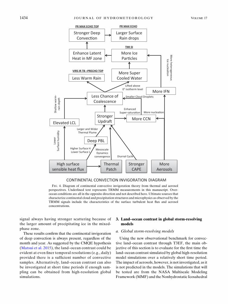
et al. 2004; WS02; Zipser et al. 2006). Figure 4 sum-

marizes the potential pathways for the invigoration of

continental deep convection based on the aforemen-

tioned previous studies presented in section 1. There

are potentially four factors that could invigorate deep

convection over land: 1) amplified CAPE; 2) high sur-

face sensible heat fluxes that lead to elevated cloud-

base heights or the height of the lifting condensation

level (HLCL), which then reduce warm cloud depth

while also deepening the PBL depth and result in en-

hanced convective width and updraft velocity; 3) the

thermal patch effect wherein islands or land-cover

patterns enhance mesoscale pressure gradients, wind

convergence, and consequently updraft velocity; and 4)

higher aerosol concentrations that can reduce warm

rain process via cloud nucleation. As evidenced from

the TRMM climatology, all of these factors potentially

can lead to the continental vigor of cloud and pre-

cipitation processes, namely, the enhancement of deep

convective processes and the concurrent suppression of

warm rain processes (Fig. 1), along with an enhanced

amount of supercooled water and more heavily rimed

ice particles (Fig. 3), which result in deeper convection

with more intense surface precipitation (Fig. 2).

Instead of using long-term climatology, this section

briefly discusses the robustness of land–ocean contrast

based on shorter time scales. Matsui et al. (2015)

proposed the idea of convection-microphysics quasi-

equilibrium (CMQE) states through a planetary view

of tropical convection. They found that the character-

istic spectrums of TRMM precipitation signals (radar

echo and microwave brightness temperature spectra),

precipitation rate, and microphysics states are nearly

identical regardless of seasons and years as long as

the sampling covered the entire tropics, regardless of

the day-to-day, seasonal, or interannual variability of

tropical dynamics.

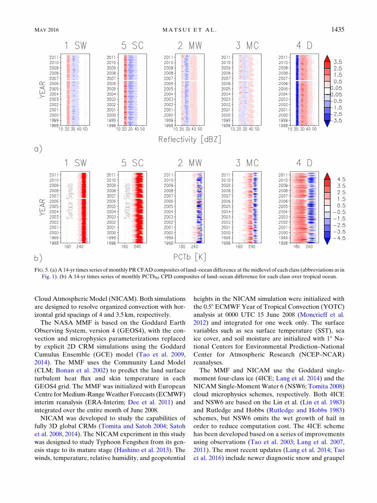
Figure 5a shows a monthly time series of the differ-

ence in composite PR CFADs for land minus ocean at

midlevels (i.e., 3 km for shallow warm and shallow cold,

3.5 km for midwarm and midcold, and 10km for deep).

There are some subtle but consistent land–ocean dif-

ferences in the shallow warm, shallow cold, and mid-

warm categories, close to the climatology difference in

Fig. 2a. The midcold category, however, shows seasonal

cycles in its land–ocean contrast. The most significant

and consistent differences appear in the deep category,

wherein continental deep clouds always show radar re-

flectivity invigoration within the solid-phase zone re-

gardless of different months and years as long as the

sampling is over the entire tropics.

Figure 5b shows a monthly time series of the differ-

ence in PCTb85 frequency between land and ocean in a

similar manner to Fig. 5a. The PCTb85 distributions

show clear land–ocean differences for all categories.

Consistent positive signals for the shallow warm and

shallow cold signals are due to land surface signals,

which are mostly likely not associated with differences

in the microphysical characteristics between land and

ocean environments. Midwarm signals are also in-

consistent throughout the time series so that there is

no time-consistent land–ocean PCTb85 because of the

lack of appreciable amounts of ice in this class. At

times, midwarm over ocean has PCTb85 probability

densities that are more narrowly distributed, but the

results are relatively sporadic. The midcold category

has more distinct land–ocean differences in PCTb85,

though the PR CFAD results are nearly identical be-

tween land and ocean. This could be because of a

difference between land and ocean in the tiny pre-

cipitating ice to which the PCTb85 is sensitive and/or

because the TMI slant beam path includes deep cate-

gory signals. The deep category has the most distinct

and consistent differences, with the overland microwave

MAY 2016 MATSU I ET AL . 1433

signal always having stronger scattering because of

the larger amount of precipitating ice in the mixed-

phase zone.

These results confirm that the continental invigoration

of deep convection is always present, regardless of the

month and year. As suggested by the CMQE hypothesis

(Matsui et al. 2015), the land–ocean contrast could be

evident at even finer temporal resolutions (e.g., daily)

provided there is a sufficient number of convective

samples. Alternatively, land–ocean contrast can also

be investigated at short time periods if enough sam-

pling can be obtained from high-resolution global

simulations.

3. Land–ocean contrast in global storm-resolvingmodels

a. Global storm-resolving models

Using the new observational benchmark for convec-

tive land–ocean contrast through T3EF, the main ob-

jective of this section is to evaluate for the first time the

land–ocean contrast simulated by global high-resolution

model simulations over a relatively short time period.

The impact of aerosols, however, is not investigated, as it

is not predicted in the models. The simulations that will

be tested are from the NASA Multiscale Modeling

Framework (MMF) and theNonhydrostatic Icosahedral

FIG. 4. Diagram of continental convective invigoration theory from thermal and aerosol

perspectives. Underlined text represents TRMM measurements in this manuscript. Over-

ocean conditions are all in the opposite direction and not described here. Ultimate sources that

characterize continental cloud and precipitation structures andmicrophysics as observed by the

TRMM signals include the characteristics of the surface turbulent heat flux and aerosol

concentrations.

1434 JOURNAL OF HYDROMETEOROLOGY VOLUME 17

Cloud Atmospheric Model (NICAM). Both simulations

are designed to resolve organized convection with hor-

izontal grid spacings of 4 and 3.5 km, respectively.

The NASA MMF is based on the Goddard Earth

Observing System, version 4 (GEOS4), with the con-

vection and microphysics parameterizations replaced

by explicit 2D CRM simulations using the Goddard

Cumulus Ensemble (GCE) model (Tao et al. 2009,

2014). The MMF uses the Community Land Model

(CLM; Bonan et al. 2002) to predict the land surface

turbulent heat flux and skin temperature in each

GEOS4 grid. The MMF was initialized with European

Centre forMedium-RangeWeather Forecasts (ECMWF)

interim reanalysis (ERA-Interim; Dee et al. 2011) and

integrated over the entire month of June 2008.

NICAM was developed to study the capabilities of

fully 3D global CRMs (Tomita and Satoh 2004; Satoh

et al. 2008, 2014). The NICAM experiment in this study

was designed to study Typhoon Fengshen from its gen-

esis stage to its mature stage (Hashino et al. 2013). The

winds, temperature, relative humidity, and geopotential

heights in the NICAM simulation were initialized with

the 0.58 ECMWFYear of Tropical Convection (YOTC)

analysis at 0000 UTC 15 June 2008 (Moncrieff et al.

2012) and integrated for one week only. The surface

variables such as sea surface temperature (SST), sea

ice cover, and soil moisture are initialized with 18 Na-

tional Centers for Environmental Prediction–National

Center for Atmospheric Research (NCEP–NCAR)

reanalyses.

The MMF and NICAM use the Goddard single-

moment four-class ice (4ICE; Lang et al. 2014) and the

NICAM Single-Moment Water 6 (NSW6; Tomita 2008)

cloud microphysics schemes, respectively. Both 4ICE

and NSW6 are based on the Lin et al. (Lin et al. 1983)

and Rutledge and Hobbs (Rutledge and Hobbs 1983)

schemes, but NSW6 omits the wet growth of hail in

order to reduce computation cost. The 4ICE scheme

has been developed based on a series of improvements

using observations (Tao et al. 2003; Lang et al. 2007,

2011). The most recent updates (Lang et al. 2014; Tao

et al. 2016) include newer diagnostic snow and graupel

FIG. 5. (a)A 14-yr times series ofmonthly PRCFADcomposites of land–ocean difference at themidlevel of each class (abbreviations as in

Fig. 1). (b) A 14-yr times series of monthly PCTb85 CPD composites of land–ocean difference for each class over tropical ocean.

MAY 2016 MATSU I ET AL . 1435

size distributions and a new frozen drops–hail cate-

gory for severe thunderstorms as well as other improve-

ments. Table 1 summarizes theMMF andNICAM setup

and physics options.

NICAM has a realistic land mask, terrain, and land-

cover specification, permitting thermal patch effects due

to sea breezes and/or land-cover heterogeneity, while

the NASA MMF only generates homogeneous surface

energy and turbulent fluxes driven by the GEOS4 CLM.

Thus, both the MMF and NICAM could be used to ex-

amine the impact of variations in the HLCL and large-

scale CAPE, while only NICAM is capable of producing

a realistic thermal patch effect (Fig. 4).

b. Satellite simulators

Model-simulated geophysical parameters (including

cloud and precipitation microphysics information) from

the MMF and the NICAM simulations are converted

into TRMM signals through the Goddard Satellite Data

Simulator Unit (G-SDSU; Matsui et al. 2013, 2014) and

the Joint Simulator for Satellite Sensors (Hashino et al.

2013). Bothmulti-instrumental simulators employ identical

microwave simulators (Kummerow 1993), radar simu-

lators (Masunaga and Kummerow 2005), and IR sim-

ulators (Nakajima and Tanaka 1986). Details on the

computation methods are described in previous studies

(Matsui et al. 2009, 2014).

Briefly, the effective dialectic function is calculated

from the Maxwell–Garnett assumption, and single

scattering properties are calculated from the Mie as-

sumption for both microwave and radar simulators.

The microwave simulator can account for slant-path

beams, mimicking the 3D slant-path observations in

conical-scanning microwave radiometers, such as the

TMI. These forward models are consistent with the

physics assumptions (including the particle size distri-

butions, phase, and effective densities) within the mi-

crophysics schemes used in the MMF and NICAM.

VIRSTbIR, PR HET, PR CFAD, and TMI PCTb85 are

simulated in each of the MMF columns and the

NICAM output and sampled in an identical manner to

the TRMM observations.

c. Simulated T3EF diagrams from the MMF andNICAM

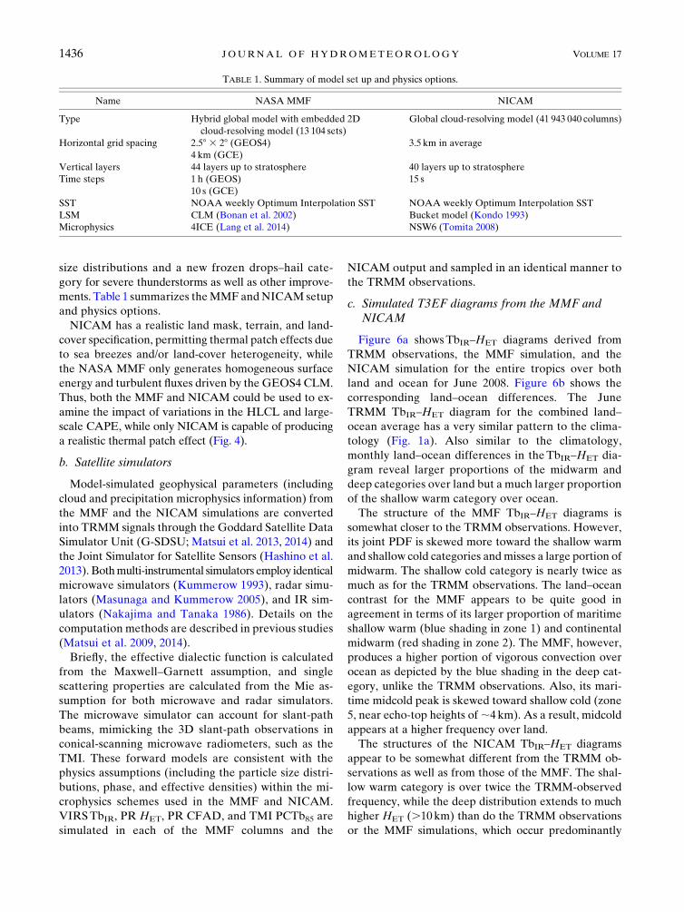
Figure 6a showsTbIR–HET diagrams derived from

TRMM observations, the MMF simulation, and the

NICAM simulation for the entire tropics over both

land and ocean for June 2008. Figure 6b shows the

corresponding land–ocean differences. The June

TRMM TbIR–HET diagram for the combined land–

ocean average has a very similar pattern to the clima-

tology (Fig. 1a). Also similar to the climatology,

monthly land–ocean differences in theTbIR–HET dia-

gram reveal larger proportions of the midwarm and

deep categories over land but a much larger proportion

of the shallow warm category over ocean.

The structure of the MMF TbIR–HET diagrams is

somewhat closer to the TRMM observations. However,

its joint PDF is skewed more toward the shallow warm

and shallow cold categories andmisses a large portion of

midwarm. The shallow cold category is nearly twice as

much as for the TRMM observations. The land–ocean

contrast for the MMF appears to be quite good in

agreement in terms of its larger proportion of maritime

shallow warm (blue shading in zone 1) and continental

midwarm (red shading in zone 2). The MMF, however,

produces a higher portion of vigorous convection over

ocean as depicted by the blue shading in the deep cat-

egory, unlike the TRMM observations. Also, its mari-

time midcold peak is skewed toward shallow cold (zone

5, near echo-top heights of;4 km). As a result, midcold

appears at a higher frequency over land.

The structures of the NICAM TbIR–HET diagrams

appear to be somewhat different from the TRMM ob-

servations as well as from those of the MMF. The shal-

low warm category is over twice the TRMM-observed

frequency, while the deep distribution extends to much

higher HET (.10km) than do the TRMM observations

or the MMF simulations, which occur predominantly

TABLE 1. Summary of model set up and physics options.

Name NASA MMF NICAM

Type Hybrid global model with embedded 2D

cloud-resolving model (13 104 sets)

Global cloud-resolving model (41 943 040 columns)

Horizontal grid spacing 2.58 3 28 (GEOS4) 3.5 km in average

4 km (GCE)

Vertical layers 44 layers up to stratosphere 40 layers up to stratosphere

Time steps 1 h (GEOS) 15 s

10 s (GCE)

SST NOAA weekly Optimum Interpolation SST NOAA weekly Optimum Interpolation SST

LSM CLM (Bonan et al. 2002) Bucket model (Kondo 1993)

Microphysics 4ICE (Lang et al. 2014) NSW6 (Tomita 2008)

1436 JOURNAL OF HYDROMETEOROLOGY VOLUME 17

under 10 km. Similar to the MMF results, there are no

distinct peaks in the midwarm and midcold zones.

NICAM produces the correct land–ocean contrast in

the form of higher frequencies over land for the deep

category and higher frequencies over ocean for the

shallow warm, though they are too strong and too

weak, respectively. The continental midwarm peak is

also quite evident, but the echo-top heights are too

shallow relative to the TRMM observations and as a

result appear as shallow warm.

Since the NICAM integration time is much shorter

than the TRMM observations and the MMF simulation,

the spatial distributions of these precipitating cloud

types are not discussed in the main article. However, the

reader is encouraged to view the detailed spatialmaps and

discussion in the supplemental material (supplement A).

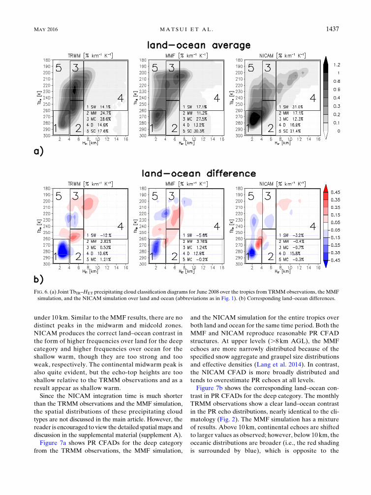
Figure 7a shows PR CFADs for the deep category

from the TRMM observations, the MMF simulation,

and the NICAM simulation for the entire tropics over

both land and ocean for the same time period. Both the

MMF and NICAM reproduce reasonable PR CFAD

structures. At upper levels (.8 km AGL), the MMF

echoes are more narrowly distributed because of the

specified snow aggregate and graupel size distributions

and effective densities (Lang et al. 2014). In contrast,

the NICAM CFAD is more broadly distributed and

tends to overestimate PR echoes at all levels.

Figure 7b shows the corresponding land–ocean con-

trast in PR CFADs for the deep category. The monthly

TRMM observations show a clear land–ocean contrast

in the PR echo distributions, nearly identical to the cli-

matology (Fig. 2). The MMF simulation has a mixture

of results. Above 10 km, continental echoes are shifted

to larger values as observed; however, below 10 km, the

oceanic distributions are broader (i.e., the red shading

is surrounded by blue), which is opposite to the

FIG. 6. (a) Joint TbIR–HET precipitating cloud classification diagrams for June 2008 over the tropics from TRMMobservations, the MMF

simulation, and the NICAM simulation over land and ocean (abbreviations as in Fig. 1). (b) Corresponding land–ocean differences.

MAY 2016 MATSU I ET AL . 1437

observations. It is probably due to the invigoration of

oceanic deep convection in the MMF simulation

(Fig. 6b). The NICAM simulation shows signs of con-

tinental invigoration above 5 km similar to the obser-

vations, but the signal is weaker than the TRMM

observations and less coherent throughout the vertical

range. In the warm precipitation zone below 5km, as

with the MMF, the results are counter to TRMM with

broader oceanic distributions. The results are discussed

more in the next section.

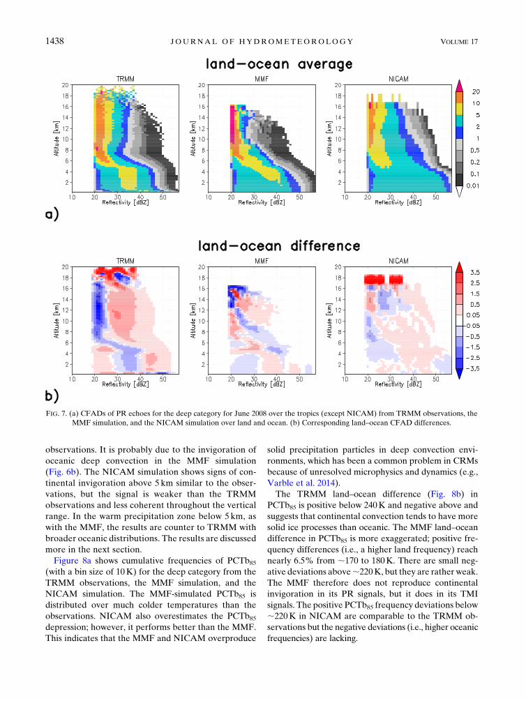
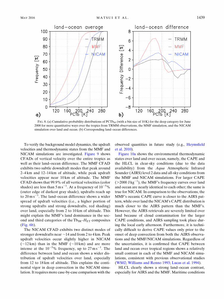
Figure 8a shows cumulative frequencies of PCTb85(with a bin size of 10K) for the deep category from the

TRMM observations, the MMF simulation, and the

NICAM simulation. The MMF-simulated PCTb85 is

distributed over much colder temperatures than the

observations. NICAM also overestimates the PCTb85depression; however, it performs better than the MMF.

This indicates that the MMF and NICAM overproduce

solid precipitation particles in deep convection envi-

ronments, which has been a common problem in CRMs

because of unresolved microphysics and dynamics (e.g.,

Varble et al. 2014).

The TRMM land–ocean difference (Fig. 8b) in

PCTb85 is positive below 240K and negative above and

suggests that continental convection tends to have more

solid ice processes than oceanic. The MMF land–ocean

difference in PCTb85 is more exaggerated; positive fre-

quency differences (i.e., a higher land frequency) reach

nearly 6.5% from ;170 to 180K. There are small neg-

ative deviations above;220K, but they are rather weak.

The MMF therefore does not reproduce continental

invigoration in its PR signals, but it does in its TMI

signals. The positive PCTb85 frequency deviations below

;220K in NICAM are comparable to the TRMM ob-

servations but the negative deviations (i.e., higher oceanic

frequencies) are lacking.

FIG. 7. (a) CFADs of PR echoes for the deep category for June 2008 over the tropics (except NICAM) from TRMM observations, the

MMF simulation, and the NICAM simulation over land and ocean. (b) Corresponding land–ocean CFAD differences.

1438 JOURNAL OF HYDROMETEOROLOGY VOLUME 17

To verify the background model dynamics, the updraft

velocities and thermodynamic states from the MMF and

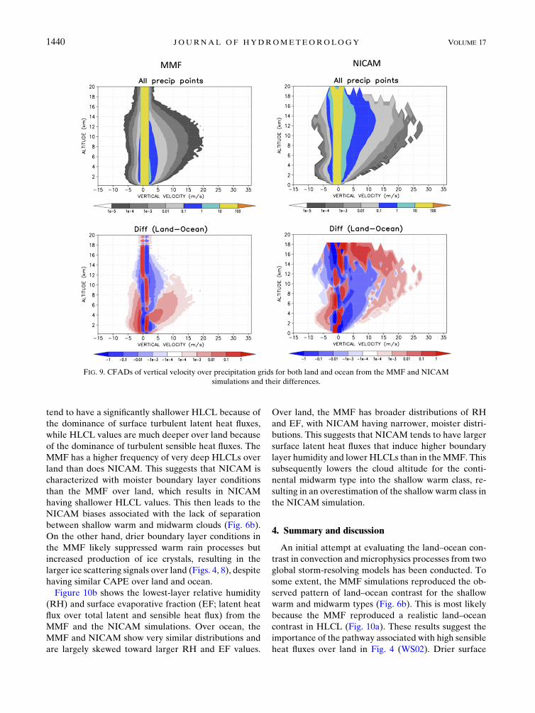
NICAM simulations are investigated. Figure 9 shows

CFADs of vertical velocity over the entire tropics as

well as their land–ocean difference. The MMF CFAD

exhibits two subtle downdraft modes that peak around

2–4 km and 12–14 km of altitude, while peak updraft

velocities appear near 10 km of altitude. The MMF

CFAD shows that 99.9% of all vertical velocities (color

shades) are less than 5m s21. At a frequency of 1025%

(outer edge of darkest gray shade), updrafts reach up

to 20m s21. The land–ocean difference shows a wider

spread of updraft velocities (i.e., a higher portion of

strong updrafts and strong downdrafts, red shading)

over land, especially from 2 to 10 km of altitude. This

might explain the MMF’s land dominance in the sec-

ond and third categories of the TbIR–HET composites

(Fig. 6b).

The NICAM CFAD exhibits two distinct modes of

stronger downdrafts near;14 and from 2 to 4 km. Peak

updraft velocities occur slightly higher in NICAM

(;12 km) than in the MMF (;10 km) and are more

intense at the 1025% frequency, up to 27m s21. The

difference between land and ocean shows a wider dis-

tribution of updraft velocities over land, especially

from 12 to 18 km of altitude. This explains the conti-

nental vigor in deep convection in the NICAM simu-

lation. It requiresmore case-by-case comparison with the

observed quantities in future study (e.g., Heymsfield

et al. 2010).

Figure 10a shows the environmental thermodynamic

states over land and over ocean, namely, the CAPE and

the HLCL in clear-sky conditions (due to the data

availability) from the Aqua Atmospheric Infrared

Sounder (AIRS) level 2 data and all-sky conditions from

the MMF and NICAM simulations. For larger CAPE

(.2000 J kg21), the MMF’s frequency curves over land

and ocean are nearly identical to each other; the same is

true for NICAM. In comparison to the observations, the

MMF’s oceanic CAPE curve is closer to the AIRS pat-

tern, while over land theNICAM’s CAPE distribution is

much closer to the AIRS pattern than the MMF’s.

However, the AIRS retrievals are severely limited over

land because of cloud contamination for the larger

CAPE conditions, and AIRS sampling took place dur-

ing the local early afternoon. Furthermore, it is techni-

cally difficult to derive CAPE values only prior to the

onset of deep convection from both the AIRS observa-

tions and the MMF/NICAM simulations. Regardless of

the uncertainties, it is confirmed that CAPE between

land and ocean over tropical regions shows a relatively

small contrast in each of the MMF and NICAM simu-

lations, consistent with previous observational studies

(WS02; Williams and Renno 1993; Lucas et al. 1994).

HLCL clearly shows a strong land–ocean contrast,

especially for AIRS and the MMF. Maritime conditions

FIG. 8. (a) Cumulative probability distributions of PCTb85 (with a bin size of 10K) for the deep category for June

2008 for more quantitative ways over the tropics from TRMM observations, the MMF simulation, and the NICAM

simulation over land and ocean. (b) Corresponding land–ocean differences.

MAY 2016 MATSU I ET AL . 1439

tend to have a significantly shallower HLCL because of

the dominance of surface turbulent latent heat fluxes,

while HLCL values are much deeper over land because

of the dominance of turbulent sensible heat fluxes. The

MMF has a higher frequency of very deep HLCLs over

land than does NICAM. This suggests that NICAM is

characterized with moister boundary layer conditions

than the MMF over land, which results in NICAM

having shallower HLCL values. This then leads to the

NICAM biases associated with the lack of separation

between shallow warm and midwarm clouds (Fig. 6b).

On the other hand, drier boundary layer conditions in

the MMF likely suppressed warm rain processes but

increased production of ice crystals, resulting in the

larger ice scattering signals over land (Figs. 4, 8), despite

having similar CAPE over land and ocean.

Figure 10b shows the lowest-layer relative humidity

(RH) and surface evaporative fraction (EF; latent heat

flux over total latent and sensible heat flux) from the

MMF and the NICAM simulations. Over ocean, the

MMF and NICAM show very similar distributions and

are largely skewed toward larger RH and EF values.

Over land, the MMF has broader distributions of RH

and EF, with NICAM having narrower, moister distri-

butions. This suggests that NICAM tends to have larger

surface latent heat fluxes that induce higher boundary

layer humidity and lower HLCLs than in theMMF. This

subsequently lowers the cloud altitude for the conti-

nental midwarm type into the shallow warm class, re-

sulting in an overestimation of the shallow warm class in

the NICAM simulation.

4. Summary and discussion

An initial attempt at evaluating the land–ocean con-

trast in convection and microphysics processes from two

global storm-resolving models has been conducted. To

some extent, the MMF simulations reproduced the ob-

served pattern of land–ocean contrast for the shallow

warm and midwarm types (Fig. 6b). This is most likely

because the MMF reproduced a realistic land–ocean

contrast in HLCL (Fig. 10a). These results suggest the

importance of the pathway associated with high sensible

heat fluxes over land in Fig. 4 (WS02). Drier surface

FIG. 9. CFADs of vertical velocity over precipitation grids for both land and ocean from the MMF and NICAM

simulations and their differences.

1440 JOURNAL OF HYDROMETEOROLOGY VOLUME 17

fluxes also elevate boundary layer heights, which would

favor the creation ofmoremidwarm clouds as shown by

the TbIR–HET diagrams (Fig. 6b). The NICAM simu-

lation tends to have much wetter surface soil condi-

tions, which induces a larger evaporative fraction and

higher relative humidity. As a result, it lowers cloud

altitudes frommidwarm to shallow warm types, resulting

in its continental midwarm (i.e., congestus) mode con-

forming more to the shallow warm category (Fig. 6b).

As a result, the NICAM simulation overestimates the

shallow warm class over the tropics (Fig. 6a). Supple-

mental material also shows extensive and excessive

distributions of shallow warm clouds over desert region

(supplement A).

Although the magnitude and extent were not quan-

titatively consistent with the observations (Fig. 8a),

both the MMF and NICAM simulations generated

more PCTb85 ice scattering in continental convection

(Fig. 8b), suggesting they produced more solid ice

particles in their deep continental convective mode

despite the large CAPE distributions being very similar

between land and ocean (Fig. 10a). However, neither

theMMF nor NICAM generated a realistic land–ocean

contrast in their radar signals as depicted by PR

CFADs (Fig. 7b). Structural differences in the simu-

lated CFADs between land and ocean are less coherent

in the vertical direction, unlike those from the TRMM

PR, which show clear, coherent patterns through solid,

mixed, and liquid-phase precipitation.

The results are also interesting because the MMF

modeling setup does not account for the thermal patch

effect. Robinson et al. (2011) concluded that meso-

scale wave dynamics due to the thermal patch effect

is the primary mechanism for continental convective

FIG. 10. (a) Frequencies of CAPE (J kg21) and HLCL (m) over ocean and land derived from AIRS level 2

retrievals, the MMF simulation, and the NICAM simulation for the large-scale environment. TheMMF results are

based on the GEOS4 grid; the NICAM CAPE and HLCL are derived from temperature and humidity fields

averaged over a 40-km footprint size, which is compatible with the AIRS level 2 retrievals. (b) Frequencies of

lowest-layer RH and surface EF over ocean and land derived from the MMF and the NICAM simulations.

MAY 2016 MATSU I ET AL . 1441

vigor over islands. At least, despite homogeneous

surface fluxes in the MMF and nearly identical CAPE

distributions between land and ocean, stronger scattering

signals were simulated in continental deep convection

primarily because of the drier surface conditions (i.e.,

higher HLCL; WS02). Of course, these results do not

reject the finding in Robinson et al. (2011), because the

MMF simulation does not reproduce more frequent

deep convection (as measured by TbIR and HET) over

land, while the NICAM simulation does. From these

simulations, it can be concluded that 1) drier surface

fluxes contribute to the generation of midwarm types of

clouds and glaciation of deep convection and 2) the

thermal patch effect is important for generating more

frequent deep convection and taller storm-top heights

in continental deep convection.

Quantifying the surface sensible heat flux impact and

thermal patch impact requires that the physics, grid

configurations, and initial and boundary conditions be-

tween the MMF and NICAM be more similar. The

overall results indicate that even these advanced global

storm-resolving modeling systems have room to im-

prove their microphysics and dynamics in order to rep-

licate the nature of the observed land–ocean contrast in

convection, as suggested by previous evaluation studies

(Masunaga et al. 2008; Inoue et al. 2010; Satoh et al.

2010; Kodama et al. 2012; Roh and Satoh 2014).

There are some pathways for improving the weak-

nesses in the simulations associated with the surface

conditions, resolution, and the sophistication of the

microphysics. The spinup of soil moisture for initial

conditions in NICAM and MMF could potentially be

improved for more realistic CAPE but would require

a more careful setup for future experiments (Mohr

2013). Although traditionally known as ‘‘cloud-resolving

models,’’ a typical grid spacing of 1–4 km and ;60

vertical levels will only resolve cloud systems greater

than ;5–40 km (Pielke 2013). Khairoutdinov et al.

(2009) showed a clear improvement in simulating

shallow/congestus populations when the horizontal

grid spacing was reduced to 200m and vertical levels

increased to 256. It is also important to couple with

realistic aerosol simulations to obtain CCN and IFN in

order to investigate whether aerosols really help to

characterize a realistic convective land–ocean con-

trast in future (Saleeby and van den Heever 2013).

It must be emphasized that analyzing global storm-

resolvingmodels provides amore comprehensive pathway

for more universal understanding, including the land–

ocean contrast. However, this approach requires a lot

more computing resources, but such an improvement is

needed to fulfill the desire to simulate a more realistic

land–ocean contrast (Lucas et al. 1994; Williams et al.

2002, 2005; WS02; Liu and Zipser 2005).

Acknowledgments. This study has been funded by the

NASA Modeling, Analysis, and Prediction (MAP) pro-

gram (Project Manager: D. Considine at NASA HQ).

Drs. T. Matsui, J. Chern, and W.-K. Tao and Mr. S. Lang

are also funded by the NASA Precipitation Measurement

Missions (PMM) program (Project Manager: R. Kakar at

NASA HQ). We also thank the NASA Advanced Super-

computing (NAS) Division (Project Manager: T. Lee at

NASA HQ) for providing the computational resources.

The lead author (T. Matsui) would like to give special

thanks to Dr. E. Zipser at the University of Utah for his

useful discussions.

REFERENCES

Awaka, J., T. Iguchi, and K. Okamoto, 1998: Early results on rain

type classification by the Tropical Rainfall MeasuringMission

(TRMM) Precipitation Radar. Proc. 8th URSI Commission F

Open Symp., Aveiro, Portugal, International Union of Radio

Science, 143–146.

Bonan, B. G., K. W. Oleson, M. Vertenstein, S. Levis, X. Zeng,

Y. Dai, R. E. Dickinson, and Z.-L. Yang, 2002: The land

surface climatology of the Community Land Model cou-

pled to the NCAR Community Climate Model. J. Climate,

15, 3123–3149, doi:10.1175/1520-0442(2002)015,3123:

TLSCOT.2.0.CO;2.

Carbone, R. E., J. D. Tuttle, D. A. Ahijevych, and S. B. Trier, 2002:

Inferences of predictability associated with warm season pre-

cipitation episodes. J. Atmos. Sci., 59, 2033–2056, doi:10.1175/

1520-0469(2002)059,2033:IOPAWW.2.0.CO;2.

Dee, D. P., and Coauthors, 2011: The ERA-Interim reanalysis:

Configuration and performance of the data assimilation sys-

tem. Quart. J. Roy. Meteor. Soc., 137, 553–597, doi:10.1002/

qj.828.

Demott, P. J., and Coauthors, 2010: Predicting global atmo-

spheric ice nuclei distributions and their impacts on climate.

Proc. Natl. Acad. Sci. USA, 107, 11 217–11 222, doi:10.1073/

pnas.0910818107.

Hashino,T.,M. Satoh,Y.Hagihara, T.Kubota, T.Matsui, T.Nasuno,

and H. Okamoto, 2013: Evaluating cloud microphysics from

NICAM against CloudSat and CALIPSO. J. Geophys. Res.

Atmos., 118, 7273–7292, doi:10.1002/jgrd.50564.

Heymsfield, G. M., L. Tian, A. J. Heymsfield, L. Li, and

S. Guimond, 2010: Characteristics of deep tropical and sub-

tropical convection from nadir-viewing high-altitude airborne

Doppler radar. J. Atmos. Sci., 67, 285–308, doi:10.1175/

2009JAS3132.1.

Iguchi, T., T. Kozu, R. Meneghini, J. Awaka, and K. Okamoto,

2000: Rain-profiling algorithm for the TRMMPrecipitation

Radar. J. Appl. Meteor., 39, 2038–2052, doi:10.1175/

1520-0450(2001)040,2038:RPAFTT.2.0.CO;2.

Inoue, T., M. Satoh, Y. Hagihara, H. Miura, and J. Schmetz, 2010:

Comparison of high-level clouds represented in a global cloud

system resolving model with CALIPSO/CloudSat and geo-

stationary satellite observations. J.Geophys. Res., 115, D00H22,

doi:10.1029/2009JD012371.

1442 JOURNAL OF HYDROMETEOROLOGY VOLUME 17

Johnson, R. H., T. M. Rickenbach, S. A. Rutledge, P. E.

Ciesielski, and W. H. Schubert, 1999: Trimodal character-

istics of tropical convection. J. Climate, 12, 2397–2418,

doi:10.1175/1520-0442(1999)012,2397:TCOTC.2.0.CO;2.

Khain, A. P., N. Benmoshe, and A. Pokrovsky, 2008: Factors de-

termining the impact of aerosols on surface precipitation from

clouds: An attempt at classification. J. Atmos. Sci., 65, 1721–1748,

doi:10.1175/2007JAS2515.1.

Khairoutdinov, M. F., S. K. Krueger, C.-H. Moeng, P. A.

Bogenschutz, andD. ARandall, 2009: Large-eddy simulation

of maritime deep tropical convection. J. Adv. Model. Earth

Syst., 1, doi:10.3894/JAMES.2009.1.15.

Kikuchi, K., and B. Wang, 2008: Diurnal precipitation regimes in

the global tropics. J. Climate, 21, 2680–2696, doi:10.1175/

2007JCLI2051.1.

Kodama, C., A. T. Noda, and M. Satoh, 2012: An assessment of the

cloud signals simulated by NICAM using ISCCP, CALIPSO,

and CloudSat satellite simulators. J. Geophys. Res., 117,

D12210, doi:10.1029/2011JD017317.

Kondo, J., 1993: A new bucket model for predicting water content

in the surface model. J. Japan Soc. Hydrol. Water Res., 6,

344–349, doi:10.3178/jjshwr.6.4_344.

Kummerow, C., 1993: On the accuracy of the Eddington approxi-

mation for radiative transfer in the microwave frequencies.

J. Geophys. Res., 98, 2757–2765, doi:10.1029/92JD02472.

Lang, S. E., W.-K. Tao, R. Cifelli, W. Olson, J. Halverson,

S. Rutledge, and J. Simpson, 2007: Improving simulations of

convective systems from TRMM LBA: Easterly and westerly

regimes. J. Atmos. Sci., 64, 1141–1164, doi:10.1175/JAS3879.1.

——, ——, X. Zeng, and Y. Li, 2011: Reducing the biases in sim-

ulated radar reflectivities from a bulk microphysics scheme:

Tropical convective systems. J. Atmos. Sci., 68, 2306–2320,

doi:10.1175/JAS-D-10-05000.1.

——,——, J.-D. Chern,D.Wu, andX. Li, 2014: Benefits of a fourth

ice class in the simulated radar reflectivities of convective

systems using a bulk microphysics scheme. J. Atmos. Sci.,

71, 3583–3612, doi:10.1175/JAS-D-13-0330.1.

Lau, K.-M., and H.-T. Wu, 2010: Characteristics of precipitation,

cloud, and latent heating associated with the Madden–

Julian oscillation. J. Climate, 23, 504–518, doi:10.1175/

2009JCLI2920.1.

Li, X., W.-K. Tao, T. Matsui, C. Liu, and H. Masunaga, 2010:

Improving a spectral bin microphysical scheme using long-

term TRMM satellite observations. Quart. J. Roy. Meteor.

Soc., 136, 382–399, doi:10.1002/qj.569.

Lin, Y.-L., R. D. Farley, and H. D. Orville, 1983: Bulk parame-

terization of the snow field in a cloud model. J. Climate Appl.

Meteor., 22, 1065–1092, doi:10.1175/1520-0450(1983)022,1065:

BPOTSF.2.0.CO;2.

Liu, C., and E. J. Zipser, 2005: Global distribution of convection

penetrating the tropical tropopause. J. Geophys. Res., 110,

D23104, doi:10.1029/2005JD006063.

Lucas, C., E. J. Zipser, and M. A. Lemone, 1994: Vertical ve-

locity in oceanic convection off tropical Australia. J. Atmos.

Sci., 51, 3183–3193, doi:10.1175/1520-0469(1994)051,3183:

VVIOCO.2.0.CO;2.

Machado, L. A. T., W. B. Rossow, R. L. Guedes, and A.W.Walker,

1998: Life cycle variations of mesoscale convective systems over

the Americas. Mon. Wea. Rev., 126, 1630–1654, doi:10.1175/

1520-0493(1998)126,1630:LCVOMC.2.0.CO;2.

Mapes, B. E., and R. A. Houze Jr., 1993: Cloud clusters and superclu-

sters over the oceanicwarmpool.Mon.Wea. Rev., 121, 1398–1416,

doi:10.1175/1520-0493(1993)121,1398:CCASOT.2.0.CO;2.

——, T. T. Warner, M. Xu, and A. J. Negri, 2003: Diurnal patterns

of rainfall in northwestern South America. Part I: Observa-

tions and context. Mon. Wea. Rev., 131, 799–812, doi:10.1175/

1520-0493(2003)131,0799:DPORIN.2.0.CO;2.

Masunaga, H., and C. Kummerow, 2005: Combined radar and ra-

diometer analysis of precipitation profiles for a parametric

retrieval algorithm. J. Atmos. Oceanic Technol., 22, 909–929,

doi:10.1175/JTECH1751.1.

——, T. S. L’Ecuyer, and C.D. Kummerow, 2005: Variability in the

characteristics of precipitation systems in the tropical Pacific.

Part I: Spatial structure. J. Climate, 18, 823–840, doi:10.1175/

JCLI-3304.1.

——, M. Satoh, and H. Miura, 2008: A joint satellite and global

CRM analysis of an MJO event: Model diagnosis. J. Geophys.

Res., 113, D17210, doi:10.1029/2008JD009986.

Matsui, T., H. Masunaga, R. A. Pielke Sr., and W.-K. Tao, 2004:

Impact of aerosols and atmospheric thermodynamics on cloud

properties within the climate system. Geophys. Res. Lett.,

31, L06109, doi:10.1029/2003GL019287.

——, X. Zeng, W.-K. Tao, H. Masunaga, W. S. Olson, and S. Lang,

2009: Evaluation of long-term cloud-resolving model simula-

tions using satellite radiance observations and multifrequency

satellite simulators. J. Atmos. Oceanic Technol., 26, 1261–1274,

doi:10.1175/2008JTECHA1168.1.

——, D. Mocko, M.-I. Lee, W.-K. Tao, M. J. Suarez, and R. A.

Pielke Sr., 2010: Ten-year climatology of summertime diurnal

rainfall rate over the conterminous U.S. Geophys. Res. Lett.,

37, L13807, doi:10.1029/2010GL044139.

——, and Coauthors, 2013: GPM satellite simulator over ground

validation sites. Bull. Amer. Meteor. Soc., 94, 1653–1660,

doi:10.1175/BAMS-D-12-00160.1.

——, and Coauthors, 2014: Introducing multisensor satellite

radiance-based evaluation for regional Earth system model-

ing. J. Geophys. Res. Atmos., 119, 8450–8475, doi:10.1002/

2013JD021424.

——,W.-K. Tao, S. J. Munchack,G. Huffman, andM.Grecu, 2015:

Satellite view of quasi-equilibrium states in tropical convec-

tion and precipitation microphysics. Geophys. Res. Lett.,

42, 1959–1968, doi:10.1002/2015GL063261.

McFarquhar,G.M., andR. List, 1991: The raindropmean free path

and collision rate dependence on rainrate for three-peak

equilibrium and Marshall–Palmer distributions. J. Atmos.

Sci., 48, 1999–2003, doi:10.1175/1520-0469(1991)048,1999:

TRMFPA.2.0.CO;2.

Mohr, K. I., W.-K. Tao, J.-D. Chern, S. V. Kumar, and C. Peters-

Lidard, 2013: The NASA-Goddard Multi-scale Mod-

eling Framework–Land Information System: Global

land/atmosphere interaction with resolved convection.

Environ. Modell. Software, 39, 103–115, doi:10.1016/

j.envsoft.2012.02.023.

Moncrieff, M. W., D. E. Waliser, M. J. Miller, M. A. Shapiro,

G. R. Asrar, and J. Caughey, 2012: Multiscale convective

organization and the YOTC virtual global field campaign.

Bull. Amer. Meteor. Soc., 93, 1171–1187, doi:10.1175/

BAMS-D-11-00233.1.

Morton, B. R., G. I. Taylor, and J. S. Turner, 1956: Turbulent

gravitational convection for maintained and instantaneous

sources. Proc. Roy. Soc. London, A234, 1–23, doi:10.1098/

rspa.1956.0011.

Nakajima, T., and M. Tanaka, 1986: Matrix formulations for the

transfer of solar radiation in a plane-parallel scattering at-

mosphere. J. Quant. Spectrosc. Radiat. Transf., 35, 13–21,

doi:10.1016/0022-4073(86)90088-9.

MAY 2016 MATSU I ET AL . 1443

Orville, R. E., and R. W. Henderson, 1986: Global distribution of

midnight lightning: September 1977 toAugust 1978.Mon.Wea.

Rev., 114, 2640–2653, doi:10.1175/1520-0493(1986)114,2640:

GDOMLS.2.0.CO;2.

Pielke, R. A., 2001: Influence of the spatial distribution

of vegetation and soils on the prediction of cumulus

convective rainfall. Rev. Geophys., 39, 151–177, doi:10.1029/

1999RG000072.

——, 2013:MesoscaleMeteorological Modeling. 3rd ed., Academic

Press, 760 pp.

Pulliainen, J., andM. Hallikainen, 2001: Retrieval of regional snow

water equivalent from space-borne passive microwave obser-

vations. Remote Sens. Environ., 75, 76–85, doi:10.1016/

S0034-4257(00)00157-7.

Robinson, F., S. Sherwood, D. Gerstle, C. Liu, and D. Kirshbaum,

2011: Exploring the land–ocean contrast in convective vigor

using islands. J. Atmos. Sci., 68, 602–618, doi:10.1175/

2010JAS3558.1.

Roh, W., and M. Satoh, 2014: Evaluation of precipitating hydro-

meteor parameterizations in a single-moment bulk micro-

physics scheme for deep convective systems over the tropical

open ocean. J. Atmos. Sci., 71, 2654–2673, doi:10.1175/

JAS-D-13-0252.1.

Rosenfeld, D., and W. L. Woodley, 2000: Deep convective clouds

with sustained supercooled liquid water down to 237.58C.Nature, 405, 440–442, doi:10.1038/35013030.

Rutledge, S. A., and P. V. Hobbs, 1983: The mesosocale and

microscale structure and organization of clouds and pre-

cipitation in midlatitude cyclones. VIII: A model for the

‘‘seeder–feeder’’ process in warm-frontal rainbands. J. Atmos.

Sci., 40, 1185–1206, doi:10.1175/1520-0469(1983)040,1185:

TMAMSA.2.0.CO;2.

Saleeby, M. S., and S. C. van den Heever, 2013: Developments in the

CSU-RAMS aerosol model: Emissions, nucleation, re-

generation, deposition, and radiation. J.Appl.Meteor.Climatol.,

52, 2601–2622, doi:10.1175/JAMC-D-12-0312.1.

Satoh,M., T.Matsuno, H. Tomita, H.Miura, T. Nasuno, and S. Iga,

2008:Nonhydrostatic icosahedral atmosphericmodel (NICAM)

for global cloud resolving simulations. J. Comput. Phys.,

227, 3486–3514, doi:10.1016/j.jcp.2007.02.006.

——, T. Inoue, and H. Miura, 2010: Evaluations of cloud prop-

erties of global and local cloud system resolving models us-

ing CALIPSO/CloudSat simulators. J. Geophys. Res., 115,

D00H14, doi:10.1029/2009JD012247.

——, and Coauthors, 2014: The Non-hydrostatic Icosahedral At-

mospheric Model: Description and development. Prog. Earth

Planet. Sci., 1, doi:10.1186/s40645-014-0018-1.

Schumacher, C., and R. A. Houze Jr., 2003: The TRMM Pre-

cipitation Radar’s view of shallow, isolated rain. J. Appl.

Meteor., 42, 1519–1524, doi:10.1175/1520-0450(2003)042,1519:

TTPRVO.2.0.CO;2.

Spencer, R.W.,H.M.Goodman, andR. E.Hood, 1989: Precipitation

retrieval over land and ocean with the SSM/I: Identification

and characteristics of the scattering signal. J. Atmos. Oceanic

Technol., 6, 254–273, doi:10.1175/1520-0426(1989)006,0254:

PROLAO.2.0.CO;2.

Stephens, G. L., and N. B. Wood, 2007: Properties of tropical

convection observed by millimeter-wave radar systems. Mon.

Wea. Rev., 135, 821–842, doi:10.1175/MWR3321.1.

——,——, and L. A. Pakula, 2004: On the radiative effects of dust

on tropical convection. Geophys. Res. Lett., 31, L23112,

doi:10.1029/2004GL021342.

Stull, R., 1988: An Introduction to Boundary Layer Meteorology.

Kluwer Academic, 818 pp.

Takahashi, T., 1978: Riming electrification as a charge generation

mechanism in thunderstorms. J. Atmos. Sci., 35, 1536–1548,doi:10.1175/1520-0469(1978)035,1536:REAACG.2.0.CO;2.

Tao, W.-K., and T. Matsui, 2015: Cloud-system resolving mod-

eling and aerosols. Encyclopedia of Atmospheric Sciences,

Vol. 4, 2nd ed. G. R. North, J. Pyle, and F. Zhang, Eds.,

Elsevier, 222–231.

——, and Coauthors, 2003: Microphysics, radiation and surface

processes in the Goddard Cumulus Ensemble (GCE)

model. Meteor. Atmos. Phys., 82, 97–137, doi:10.1007/

s00703-001-0594-7.

——, X. Li, A. Khain, T. Matsui, and S. Lang, 2007: Role of at-

mospheric aerosol concentration on deep convective pre-

cipitation: Cloud-resolving model simulations. J. Geophys.

Res., 112, D24S18, doi:10.1029/2007JD008728.

——, and Coauthors, 2009: A multiscale modeling system: De-

velopments, applications, and critical issues.Bull. Amer.Meteor.

Soc., 90, 515–534, doi:10.1175/2008BAMS2542.1.

——, J.-P. Chen, Z. Li, C. Wang, and C. Zhang, 2012: Impact of

aerosols on convective clouds and precipitation.Rev. Geophys.,

50, RG2001, doi:10.1029/2011RG000369.

——, and Coauthors, 2014: The Goddard Cumulus Ensemble model

(GCE): Improvements and applications for studying pre-

cipitation processes.Atmos. Res., 143, 392–424, doi:10.1016/j.atmosres.2014.03.005.

——, D. Wu, S. Lang, J.-D. Chern, C. Peters-Lidard, A. Fridlind,

and T. Matsui, 2016: High-resolution NU-WRF simulations of

a deep convective-precipitation system duringMC3E: Further

improvements and comparisons between Goddard micro-

physics schemes and observations. J. Geophys. Res. Atmos.,

121, 1278–1305, doi:10.1002/2015JD023986.

Tomita, H., 2008: New microphysics with five and six categories

with diagnostic generation of cloud ice. J. Meteor. Soc. Japan,

86A, 121–142, doi:10.2151/jmsj.86A.121.

——, and M. Satoh, 2004: A new dynamical framework of non-

hydrostatic global model using the icosahedral grid. Fluid

Dyn. Res., 34, 357–400, doi:10.1016/j.fluiddyn.2004.03.003.

Varble,A., andCoauthors, 2014: Evaluation of cloud-resolving and

limited area model intercomparison simulations using TWP-

ICE observations: 1. Deep convective updraft properties.

J. Geophys. Res. Atmos., 119, 13891–13918, doi:10.1002/

2013JD021371.

Wall, C., C. Liu, and E. Zipser, 2013: A climatology of tropical

congestus using CloudSat. J. Geophys. Res. Atmos., 118,

6478–6492, doi:10.1002/jgrd.50455.

Wallace, J. M., 1975: Diurnal variations in precipitation and thun-

derstorm frequency over the conterminous United States. Mon.

Wea. Rev., 103, 406–419, doi:10.1175/1520-0493(1975)103,0406:

DVIPAT.2.0.CO;2.

Wang, J.-J., R. F. Adler, G. J. Huffman, and D. Bolvin, 2014: An

updated TRMM composite climatology of tropical rainfall

and its validation. J. Climate, 27, 273–284, doi:10.1175/

JCLI-D-13-00331.1.

Williams, E., and N. Renno, 1993: An analysis of the condi-

tional instability of the tropical atmosphere. Mon. Wea.

Rev., 121, 21–36, doi:10.1175/1520-0493(1993)121,0021:

AAOTCI.2.0.CO;2.

——, and S. Stanfill, 2002: The physical origin of the land–ocean

contrast in lightning activity. C. R. Phys., 3, 1277–1292,

doi:10.1016/S1631-0705(02)01407-X.

1444 JOURNAL OF HYDROMETEOROLOGY VOLUME 17

——, and Coauthors, 2002: Contrasting convective regimes over the

Amazon: Implications for cloud electrification. J. Geophys.

Res., 107, 8082–8101, doi:10.1029/2001JD000380.

——, T. Chan, and D. Boccippio, 2004: Islands as miniature con-

tinents: Another look at the land–ocean lightning contrast.

J. Geophys. Res., 109, D16206, doi:10.1029/2003JD003833.

——,V.Mushtak,D.Rosenfeld, S.Goodman, andD.Boccippio, 2005:

Thermodynamic conditions favorable to superlative thunder-

storm updraft, mixed phase microphysics and lightning flash rate.

Atmos. Res., 76, 288–306, doi:10.1016/j.atmosres.2004.11.009.

Yuter, S. E., and R. A. Houze Jr., 1995: Three-dimensional

kinematic and microphysical evolution of Florida cumulo-

nimbus. Part II: Frequency distributions of vertical velo-

city, reflectivity, and differential reflectivity. Mon. Wea.

Rev., 123, 1941–1963, doi:10.1175/1520-0493(1995)123,1941:

TDKAME.2.0.CO;2.

Zipser, E. J., C. Liu, D. J. Cecil, S. W. Nesbitt, and D. P. Yorty,

2006: Where are the most intense thunderstorms on

Earth? Bull. Amer. Meteor. Soc., 87, 1057–1071, doi:10.1175/

BAMS-87-8-1057.

MAY 2016 MATSU I ET AL . 1445