on the dynamics of flexible risers and suspended …

ON THE DYNAMICS OF FLEXIBLE RISERS AND SUSPENDED PIPES SiSgS

by

Farman BARADARAN-S EYED

Thesis Submitted for the Degree of Doctor of Philosophy in the University of London

Department of Mechanical Engineering University College London

September 1989

ProQuest Number: 10609095

All rights reserved

INFORMATION TO ALL USERS The quality of this reproduction is dependent upon the quality of the copy submitted.

In the unlikely event that the author did not send a com p le te manuscript and there are missing pages, these will be noted. Also, if material had to be removed,

a note will indicate the deletion.

uestProQuest 10609095

Published by ProQuest LLC(2017). Copyright of the Dissertation is held by the Author.

All rights reserved.This work is protected against unauthorized copying under Title 17, United States C ode

Microform Edition © ProQuest LLC.

ProQuest LLC.789 East Eisenhower Parkway

P.O. Box 1346 Ann Arbor, Ml 48106- 1346

ABSTRACT

This thesis describes a theoretical and numerical study of the static and dynamic behaviour of flexible pipes and risers. Although the effects of conventional loadings due to self-weight, current, waves and surface vessel excitation are included, this work is specifically aimed at identifying the effects of internal and external fluid pressures as well as both constant density and alternating gas-fluid internal flows on the static and dynamic behaviour of risers. Particular emphasis is placed on research and development of advanced numerical analysis methods for solving the non-linear riser equations in the frequency and time domains. Theoretically calculated responses have been compared with results of model tests carried out at Heriot-Watt University and University College London and with theoretical predictions from alternative formulations. Modified forms of the governing equations for flexible risers have been derived from first principles to include the effects of internal and external hydrostatic pressures and a steady internal flow. It is rigorously shown that the conventional derivation of effective tension using a buoyancy analogy is equivalent to that obtained through exact integration of fluid pressures over the curved surface of the riser pipe. It is also demonstrated that the effect of a steady internal flow is analogous to that of hydrostatic pressure and may be included in the governing equations through the effective tension term.

The riser governing equations have been solved using a finite element analysis program written specifically for flexible risers and similar pipe geometries. The static analysis of the riser is carried out using an iterative approach that can accommodate general loading conditions using an incremental shifting procedure. Modifications to the standard non-linear static analysis techniques have been proposed and are shown to provide a more accurate representation of the deformation dependence of loading whilst retaining the non-linear influence of tensile forces on pipe geometry. Dynamic analyses have been carried out using both frequency and time domain techniques. The frequency domain approach is a regular wave analysis based on a combined wave and current linearisation whilst the time domain analysis uses the Newmark-/?

-4-

method and can accommodate regular and irregular sea states as well as geometric non-linearities. Results of this numerical work have been verified by comparison with model tests and analysis results from several sources. Model tests carried out at Heriot-Watt University at 1:50th. scale have been used to verify global predictions for riser responses and tensile forces. Specially designed model tests at University College London have been used to confirm the validity of predicted riser responses to internal flow. Comparisons have also been made with the analysis results of parallel research works. Case studies of typical North Sea flexible risers are presented.

The analytical and numerical work demonstrates that it is essential to include the effects of internal and external hydrostatic pressures and internal flow for accurate prediction of the overall response of a flexible riser. In particular, internal flow composed of alternating gas-liquid phases (slug flow) is shown to induce large oscillations in riser tensions at frequencies defined by the flow parameters. These oscillations are comparable to those induced by wave action and have a significant impact on the fatigue life of flexible risers.

To my parents Haydar and Farideh

-7-

ACKNOWLEDGMENTS

The author is greatly indebted to Professor M H Patel whose excellent supervision and keen guidance made this work possible.

The financial support of the Science and Engineering Research Council (SERC) towards projects funding this work is acknowledged.

Special thanks are due to Dr. G J Lyons and Mr. A Holland of University College London, and also Mr. G Hartnup of Heriot Watt University who most kindly supplied experimental results for comparison studies in this work.

Dr. S M Hung, Dr. A P Blackie and Mr. P Sincock are thanked for their extensive advice on word-processing of this document. The author ows a great deal to Mr. S Sarohia for the use of his excellent graph plotting package.

The author wishes to extend special thanks to Dr. A Kyriacou, Mr. B Hogan and Mr. M Iline whose friendship, help and encouragement has been invaluable.

Finally, members of staff at the Santa-Fe Laboratories for Offshore Engineering at University College London are thanked for their support throughout this work.

-9-

CONTENTSABSTRACT 3ACKNOWLEDGMENTS 7CONTENTS 9LIST OF FIGURES 12LIST OF TABLES 22NOTATION 25

1 - INTRODUCTION 28

1.1 - Marine Risers 281.2 - Historical Background on Flexible Risers 291.3 - Construction of Flexible Risers 311.4 - Flexible Riser Configurations 321.5 - Problems in Analysis of Flexible Risers 36

2 - LITERATURE REVIEW 45

2.1 - Static Analysis Methods 452.2 - Dynamic Analysis Methods (Frequency Domain) 542.3 - Dynamic Analysis Methods (Time Domain) 632.4 - Influence of Boundary Conditions 702.5 - Internal and External Pressure Forces 732.6 - Internal Flow Effects 76

3 - GOVERNING EQUATIONS 79

3.1 - Introduction 793.2 - Pressure Forces in Two Dimensions 82

3.2.1 - Equations for a Straight Pipe 823.2.2 - Approximate Equations for Curved Pipes 853.2.3 - Exact Equations for Curved Pipes 89

3.3 - Pressure Forces in Three Dimensions 933.4 - Internal Flow Forces in Two Dimensions 1023.5 - Internal Flow Forces in Three Dimensions 1053.6 - Governing Equations 106

3.6.1 - Equations for Flexible Pipes 1063.6.2 - Equations for Rigid Vertical Pipes 1093.6.3 - Equations for Rigid Horizontal Pipes 109

-10-

4 - ANALYTICAL SOLUTIONS 118

4.1 - Introduction 1184.2 - Elastic Catenary Equations 1224.3 - Pipelaying Equations 1254.4 - Steep-S Risers 1294.5 - Lazy-S Risers 1314.6 - Steep-Wave Risers 1324.7 - Lazy-Wave Risers 1334.8 - Towed Pipelines 135

5 - FINITE ELEMENT STATIC ANALYSIS 156

5.1 - Introduction 1565.2 - The Finite Element Method 161

5.2.1 - Matrix Equations of Equilibrium 1615.2.2 - Boundary Conditions 1665.2.3 - Prescribed Nodal Displacements 166

5.3 - Static Loads on the Pipe 1685.4 - Solution of Non-linear Equations 169

5.4.1 - Direct Iteration Method 1695.4.2 - Improved Direct Iteration Method 1705.4.3 - Incremental Solution Technique

(Deferred Averaging) 1725.4.4 - Hybrid Methods 1745.4.5 - Incremental Shifting Procedure 175

6 - FINITE ELEMENT DYNAMIC ANALYSIS 203

6.1 - Introduction 2036.2 - Dynamic Equations of Motion 2076.3 - Description of the Sea State 2096.4 - Regular Wave Analysis in the Frequency Domain 2136.5 - Regular Slug Flow Analysis in the Frequency Domain 2256.6 - Time Domain Analysis 2286.7 - Non-linear Analysis in the Time Domain 2346.8 - Regular Slug Flow Analysis in the Time Domain 237

-11-

7 - VERIFICATION OF ANALYSIS 253

7.1 - Comparison with Analytical Solutions 2537.2 - Model Tests at Heriot-Watt University 255

7.2.1 - Tests with Fixed Top Connection 2577.2.2 - Tests with Vessel Motions 258

7.3 - Model Tests at University College London 2617.3.1 - Tests under Internal Pressure 2627.3.2 - Tests with Internal Flow 263

7.4 - Comparison with Other Works 266

8 - APPLICATION STUDIES 346

8.1 - Introduction 3468.2 - Application Studies 348

8.2.1 - Selection of Buoy Upthrust 3488.2.2 - Selection of Buoy Height 3508.2.3 - Vessel Offset Limitations 3528.2.4 - Relative Contribution of Vessel Motions to

Pipe Response 3538.2.5 - Surface Piercing Risers 3538.2.6 - Static Analysis Methods 3548.2.7 - Numerical Difficulties with Pipes of Low

Flexural Rigidity 3578.2.8 - Out of Plane Deformation Under Static Current 3588.2.9 - Wave and Current Superposition 3598.2.10 - Comparison of frequency and Time Domain

Solutions 3608.2.11 - Risers Response to Different Wave Headings 3628.2.12 - Riser Response to Irregular Sea States 3648.2.13 - Non-linear Seabed Boundary Condition 3668.2.14 - Combined Wave, Vessel and Internal Flow

Induced Excitation 366

9 - CONCLUSIONS 439

REFERENCES 444

-12-

LIST OF FIGURES

CHAPTER 1 Page

1.1 - Rigid and Flexible Riser Geometries 391.2 - Enchova Field Layout 401.3 - Badejo Early Production System 401.4 - Balmoral Field Layout 411.5 - Cadlao CALM Buoy System 411.6 - Petrojarl-1 Floating Production System 421.7 - Typical Flexible Pipe Cross Section 431.7 - Typical Flexible Pipe End Connector Cross Section 44

CHAPTER 3 Page

3.1 - Straight Pipe Element 1113.2 - Curved Pipe Element for Approximate Analysis 1123.3 - Buoyancy Model for Pressure Forces 1133.4 - Curved Pipe Element for Exact Analysis 1143.5 - Torus Geometry 1153.6 - Local Torus Co-ordinate System in Three Dimensions 1163.7 - Forces on a Curved Pipe Section 117

CHAPTER 4 Page

4.1 - Elastic Catenary Model 1464.2 - Simple Catenary Riser Model 1474.3 - Steep-S Riser Geometry 1484.4 - Flow-chart for Calculation of the Steep-S Profile 1494.5 - Lazy-S Riser Geometry 1504.6 - Flow-chart for Calculation of the Lazy-S Profile 1514.7 - Steep-wave Riser Geometry 1524.8 - Lazy-wave Riser Geometry 1534.9 - Towed Pipeline Model 1544.10 - Comparison of Catenary and parabolic profiles for

Different Pipe Lengths 155

-13-

CHAPTER 5 Page

5.1 - Shape functions for an Eneastree Element 1795.2 - Shape functions for an Element Pinned at Node (1) 1805.3 - Shape functions for an Element Pinned at Node (2) 1815.4 - Stiffness Matrix for an Encastree Element 1825.5 - Stiffness Matrix for an Element Pinned at Node (1) 1835.6 - Stiffness Matrix for an Element Pinned at Node (2) 1845.7 - Geometric Stiffness Matrix for an Encastree Element 1855.8 - Geometric Stiffness Matrix for an Element Pinned at

Node (1) 1865.9 - Geometric Stiffness Matrix for an Element Pinned at

Node (2) 1865.10 - Improved Geometric Stiffness Matrix for an Encastree

Element 1875.11 - Equivalent Nodal Loads for a Uniform Trapezoidal Load

on an Encastree Element 1895.12 - Equivalent Nodal Loads for a Partial Trapezoidal Load

on an Encastree Element 1905.13 - Equivalent Nodal Loads for a Point Load on an Encastree

Element 1915.14 - Equivalent Nodal Loads for a Partial Trapezoidal Load

on an Element Pinned at Node (1) 1925.15 - Equivalent Nodal Loads for a Partial Trapezoidal Load

on an Element Pinned at Node (2) 1935.16 - Static Boundary Conditions 1945.17 - Direct Iteration Method Schematic 1955.18 - Flow-chart for Static Analysis with Direct Iteration

Method 1965.19 - Improved Direct Iteration Method Schematic with

Deformation Dependent Loading 1975.20 - Flow-chart for Static Analysis with Improved Direct

Iteration Method 1985.21 - Incremental Method Schematic 1995.22 - Incremental Method Schematic with Deferred Averaging 2005.23 - Flow-chart for Static Analysis with Incremental Method

using Deferred Averaging 2015.24 - Hybrid Method Schematic 202

-14-

CHAPTER 6 Page

6.1 - Linearisation Results from Krolikowski (1980) 2436.2 - Dynamic Boundary Conditions 2446.3 - Element Mass Matrix 2456.4 - Element Added Mass Matrix 2466.5 - Linear Wave Profile and Notations 2476.6 - Wave Height Spectrum 2486.7 - Rayleigh Proportional Damping 2496.8 - Linearised Drag Force Vector 2506.9 - Linearised Drag Damping Matrix 2516.10 - Inertia Force Vector 252

CHAPTER 7 Page

7.1 - Buoy Geometry in Heriot-Watt Model Tests 2857.2 - Comparison of Static Profiles from Heriot-Watt Model

Tests and REFLEX (Fixed Top) 2867.3 - Comparison of Dynamic Displacements from Heriot-Watt

Model Test 1 and REFLEX 2877.4 - Comparison of Dynamic Displacements from Heriot-Watt









Model Test 10 and REFLEX 2967.13 - Heriot-Watt Time History 1 297

-15-

7.14 - Heriot-Watt Time History 2 2977.15 - Heriot-Watt Time History 3 2977.16 - Heriot-Watt Time History 4 2987.17 - Heriot-Watt Time History 5 2987.18 - Heriot-Watt Time History 6 2987.19 - Heriot-Watt Time History 7 2997.20 - Heriot-Watt Time History 8 2997.21 - Heriot-Watt Time History 9 3007.22 - Heriot-Watt Time History 10 3007.23 - Comparison of Static Profiles from Heriot-Watt Model

Tests and REFLEX (Vessel Motion) 3017.24 - Comparison of Dynamic Displacements from Heriot-Watt

Model Test V-l and REFLEX 3027.25 - Comparison of Dynamic Displacements from Heriot-Watt

Model Test V-2 and REFLEX 3037.26 - Comparison of Dynamic Displacements from Heriot-Watt






Model Test V-8 and REFLEX 3097.32 - Heriot-Watt Time History V-l 3107.33 - Heriot-Watt Time History V-2 3107.34 - Heriot-Watt Time History V-3 3117.35 - Heriot-Watt Time History V-4 3117.36 - Heriot-Watt Time History V-5 3127.37 - Heriot-Watt Time History V-6 3127.38 - Heriot-Watt Time History V-7 3137.39 - Heriot-Watt Time History V-8 3137.40a- Internal Flow Test Arrangement 3147.40b- UCL Riser and Tether Tank 3157.41 - Displaced Riser Profiles for UCL Pressure Test 1 3167.42 - Displaced Riser Profiles for UCL Pressure Test 2 316

-16-

7.43 - Displaced Riser Profiles for UCL Pressure Test 3 3167.44 - Displaced Riser Profiles for UCL Pressure Test 4 3167.45 - Displaced Riser Profiles for UCL Pressure Test 5 3177.46 - Displaced Riser Profiles for UCL Pressure Test 6 3177.47 - Displaced Riser Profiles for UCL Riser Tank Pressure

Test 1 3177.48 - Displaced Riser Profiles for UCL Riser Tank Pressure

Test 2 3177.49 - Displaced Riser Profiles for UCL Internal Flow Test 1 3187.50 - Displaced Riser Profiles for UCL Internal Flow Test 2 3187.51 - Displaced Riser Profiles for UCL Internal Flow Test 3 3187.52 - Displaced Riser Profiles for UCL Internal Flow Test 4 3187.53 - Displaced Riser Profiles for UCL Riser Tank Internal

Flow Test 1 3197.54 - Displaced Riser Profiles for UCL Riser Tank Internal

Flow Test 2 3197.55 — Comparison of Dynamic Displacements for UCL Internal

Flow Test 1 3197.56 - Comparison of Dynamic Displacements for UCL Internal



Flow Test 4 3207.59 - Comparison of Dynamic Displacements for UCL Riser

Tank Internal Flow Test 1 3207.60 - Comparison of Dynamic Displacements for UCL Riser

Tank Internal Flow Test 2 3207.61 - Displacement Time History for UCL Internal Flow

Test 1 3217.62 - Displacement Time History for UCL Internal Flow



Test 4 3227.65 - Displacement Time History for UCL riser Tank

Internal Flow Test 1 3237.66 - Displacement Time History for UCL riser Tank

-17-

Internal Flow Test 27.67 - Comparison of Static Profiles for Simple Catenary

Case Study by McNamara (1986)7.68 - Comparison of Static Tensile Forces for Simple Catenary

Case Study by McNamara (1986)7.69 - Comparison of Static Bending Moments for Simple

Catenary Case Study by McNamara (1986)7.70 - Comparison of Displacements Envelope for Steep-S Case

Study by McNamara (1986)7.71 - Comparison of Bending Moment Variations for Steep-S

Case Study by McNamara (1986)7.72 - Comparison of Natural Periods from REFLEX and Owen(1986)7.73 - Comparison of Geometries for Owen (1986) Case Study

with Current and Vessel Excursion7.74 - Comparison of Displacements Envelope for Owen (1986)

without Vessel Motions7.75 - Comparison of Displacements Envelope for Owen (1986)

with Vessel Motions7.76 - Comparison of In-plane Profiles with O'Brien (1988)7.77 - Comparison of Out of Plane Profiles with O'Brien (1988)7.78 - Comparison of Tensile Forces with O'Brien (1988)7.79 - Comparison of Bending Moments with O'Brien (1988)7.80 - Comparison of Out of Plane Bending Moments with

O'Brien (1988)7.81 - Riser Torques For case Study By O'Brien (1988)7.82 - Incremental Shifting for Calculation of Static Profile

due to Mathisen (1986) and Engseth (1988)7.83 - Comparison of Multiple catenary Solution for Static

Profile with Mathisen (1986) and Engseth (1988)7.84 - Comparison of Effective Tensions with Engseth (1988)7.85 - Comparison of Bending Moments with Engseth (1988)7.86 - Natural Frequencies of Vibration for Towed pipeline

Case Study7.87 - Dynamic Vertical Displacements for Towed Pipeline

Case Study7.88 - Bending Moment Variations for Towed Pipeline Case Study7.89 - Modal Participation Parameters for Towed Pipeline

Case Study

323

324

325

326

327

328329

330

331

332333334335336

337338

339

340341342

343

344344

345

-18-

CHAPTER 8 Page

8.1 - Steep-S Motion Sensitivity to Buoy Upthrust 3708.2 - Steep-wave Motion Sensitivity to Buoy Upthrust 3718.3 - Lazy-S Motion Sensitivity to Buoy Upthrust 3728.4 - Lazy-wave Motion Sensitivity to Buoy Upthrust 3738.5 - Lazy-wave Profile Sensitivity to Changes in Internal

Fluid Density 3748.6 - Steep-S Motion Sensitivity to Buoy Height Above Seabed 3758.7 - Steep-wave Motion Sensitivity to Buoy Height Above

Seabed 3768.8 - Lazy-S Motion Sensitivity to Buoy Height Above Seabed 3778.9 - Steep-S Tensile Force Sensitivity to Vessel Motions for

Different Buoy Heights Above Seabed 3788.10 - Steep-wave Tensile Force Sensitivity to Vessel Motions

for Different Buoy Heights Above Seabed 3798.11 - Lazy-S Tensile Force Sensitivity to Vessel Motions for

Different Buoy Heights Above Seabed 3808.12 - Steep-S Natural Period Sensitivity to Buoy Height Above

Seabed 3818.13 - Lazy-S Natural Period Sensitivity to Buoy Height Above

Seabed 3828.14 - Steep-S Natural Period Sensitivity to Horizontal Vessel

Offset 3838.15 - Lazy-S Natural Period Sensitivity to Horizontal Vessel

Offset 3848.16 - Lazy-wave Motion Sensitivity to Horizontal Separation 3858.17 - Steep-S Sensitivity to Vessel Surge and Heave Motions 3868.18 - Steep-wave Sensitivity to Vessel Surge and Heave Motions 3878.19 - Lazy-S Sensitivity to Vessel Surge and Heave Motions 3888.20 - Sensitivity of Riser Tensile Forces to Change in Riser

Effective Weight Above Water Line 3898.21 - Effect of Non-linearities on Riser Static Profile Under

Current (EA/EI=340) 3908.22 - Effect of Non-linearities on Riser Static Tensions Under

Current (EA/EI=340) 391

-19-

8.23

8.24

8.25

8.26

8.27

8.28

8.298.308.318.328.338.348.358.36

8.37

8.38

8.39

8.408.41

8.42

8.43

8.44

8.45

Effect of Non-linearities on Riser Static Shear Forces Under Current (EA/EI=»340) 392Effect of Non-linearities on Riser Static Bending Moments Under Current (EA/EI=340) 393Effect of Non-linearities on Riser Static Profile Under Current (EA/EI-34000) 394Effect of Non-linearities on Riser Static Tensions Under Current (EA/EI-34000) 395

• Effect of Non-linearities on Riser Static Shear Forces Under Current (EA/EI-34000) 396Effect of Non-linearities on Riser Static Bending Moments Under Current (EA/EI-34000) 397

• Riser In-plane Profile Under Cross Current 398■ Riser Out of Plane Profile Under Cross Current 399• Riser Plan Under Cross Current 400• Riser Tensions Under Cross Current 401• Riser In-plane Bending Moments Under Cross Current 402■ Riser Out of Plane Bending Moments Under Cross Current 403■ Riser Torsions Under Cross Current 404■ Comparison of Dispalcement Envelopes using Static and Dynamic Current Models 405

■ Comparison of Tensile Forces with Different Current and Wave Combinations 406

■ Comparison of Displacement Envelopes with Different Current and Wave Combinations 407

- Comparison of Forces and Moments with Different Currentand Wave Combinations 408

- Comparison of Frequency and Time Domain Solutions 409- Response Time Histories at Sagbend in 20m, 16sRegular Seas 410

- Riser In-plane Displacements Envelope for Different Wave Headings 411

- Side View of Riser Displacements Envelope for Different Wave Headings 412

- Plan View of Riser Displacements Envelope for Different Wave Headings 413

- Riser Tensile Force Envelope for Different Wave Headings 414

-20-

8.468.47

8.48

8.498.50

8.51

8.52

8.538.54

8.55

8.56

8.57

8.588.598.60

8.618.628.638.64

8.65

8.66

8.67

• Riser Torsion Envelope for Different Wave Headings 415■ Riser Out of Plane Bending Moment Envelope for Different Wave Headings 416

■ Riser In-plane Bending Moment Envelope for DifferentWave Headings 417

■ Moment Time Histories at SWL for Different Wave Headings 418■ Moment Time Histories at Sagbend for Different Wave Headings 419

■ Moment Time Histories at Arch Top for Different Wave Headings 420

■ Moment Time Histories at Start of Buoyancy for Different Wave Headings 421

■ JONSWAP Spectrum for 7m Significant, 10s Sea State 422■ Vessel Surge Characteristics for Irregular Wave CaseStudy 423

■ Vessel Heave Characteristics for Irregular Wave Case 424 Study

- Vessel Pitch Characteristics for Irregular Wave CaseStudy 425

■ Vessel Surge, Heave, Pitch Time Histories in IrregularSeas 426

■ Displacement Time Histories at SWL in Irregular Seas 427■ Displacement Time Histories at Sagbend in Irregular Seas 428■ Displacement Time Histories at Arch Top in IrregularSeas 429

■ Lazy-wave Response in 12m, 20s Regular Seas 430■ Bounds of Tensile Forces in 12m, 20s Regular Seas 431■ Bounds of Bending Moments in 12m, 20s Regular Seas 431- Combined Wave, Vessel and Slug Induced Dynamics in5s Regular Sea State 432

- Combined Wave, Vessel and Slug Induced Dynamics in10s Regular Sea State 433



-21-

8.68 - Combined Wave, Vessel and Slug Induced Dynamics in5s Regular Sea State

8.69 - Typical Tensile Force Envelopes for Wave, Vessel andSlug Induced Dynamics in 25s Regular Seas

8.70 - Typical Bending Moment Envelopes for Wave, Vessel andSlug Induced Dynamics in 25s Regular Seas

436

437

438

-22-

LIST OF TABLES

CHAPTER 7 Page

7.1 - Data for the Heriot-Watt University model test riserwith a fixed top connection 274

7.2 - Combination of wave heights and periods used withHeriot-Watt University model tests on a steep-S riser with a fixed top connection 274

7.3 - Comparison of variations in top tension fromHeriot-Watt fixed top tests and REFLEX 275

7.4 - Comparison of variations in base tension fromHeriot-Watt fixed top tests and REFLEX 275

7.5 - Data used in modelling the Heriot-Watt University modeltest riser with vessel motions 276

7.6 - Combination of wave heights, periods and vessel transferfunctions used at Heriot-Watt University model testswith vessel motions 276

7.7 - Comparison of variations in top tension from Heriot-Wattmodel tests with vessel motion and REFLEX 277

7.8 - Calculated natural frequencies of model steep-S riserused in Heriot-Watt tests with vessel motions 277

7.9 - Properties and dimensions of tube used in UCL tests 2787.10 - Geometry used in UCL static pressure tests 2787.11 - Geometry used in UCL internal flow tests 2787.12 - Flow data for UCL internal flow tests 2787.13 - Data for simple catenary case study by McNamara(1986) 2797.14 - Comparison of pipe end reactions and angles for the

subsea tower case study by McNamara(1986) 2807.15 - Data for steep-S flexible riser case study by McNamara

(1986) 2817.16 - Data for case study by Owen(1986) 2817.17 - Data for case study by 0'Brien(1988) 2827.18 - Data for case study by Mathisen(1986) and Engseth(1988) 2837.19 - Data for towed pipeline analysis 284

-23-

CHAPTER 8 Page

8.1 - General pipe and buoyancy data for case studies 3688.2 - Geometric data for the steep-wave case study 3688.3 - Geometric data for the lazy-wave case study with seabed 369

contact8.4 - Geometric data for the lazy-S case study with internal

flow 369

-25-

NOTATION

A - Cross sectional areaB - Global damping matrixb - Element drag damping matrixBs - Global structural damping matrixbg - Element structural damping matrix

- Coefficient of dragCc - Equivalent linearised drag coefficient for steady currentC^ - Equivalent linearised drag coefficient for wave loadingC - Coefficient of added inertia md - Water depth F - Global force vector f - Element force vector f^ - Element drag force vector£eff- Effective force vector in time domain analysisf. - Element inertia force vector — 1

f - Element internal-flow induced force vector “sg - Acceleration due to gravityH - Pressure headH0 - Horizontal tensionI - Identity matrixi - Unit vector along x axisI - Element polar moment of inertiaj - Unit vector along y axisK - Global stiffness matrixk - Unit vector along z axisk - Wave numberk - Element stiffness matrix^ - Element axial stiffness matrixK ££- Effective global stiffness matrix in time domain analysisk^ - Element flexural stiffness matrixk - Element geometric stiffness matrix §L - Element lengthM - Global mass matrixm - Element mass matrixMs - Global structural mass matrixm - Element axial and flexural mass matrix—sm - Element torsional mass matrix

-26-

n - Unit normal to surface0 - Centre of curvatureP - PressureQ - Volume flow rateR - Pipe radiusr - Radius of curvatures - ArclengthS^- Spectral density of wave height T - TensionT - Transformation matrixt - TimeU - Fluid velocityu - Time variant fluid velocity along x axisuc - Current velocityu^ - Magnitude of pipe relative velocityV - Shear forcev - Time variant fluid velocity along y axisw - Weight per unit length of pipeX - Displacement vector0 - Null matrix or vector

GREEK SYMBOLS

a - Parameter of Newmark-/9 methoda - Mass matrix multiplier in structural damping calculationsP - Stiffness matrix multiplier in structural damping calculations e - Strain; Error tolerance6 - Angle of element from the x axis0^ - Angle at the base of pipe8 - Angle at the top of pipe$ - Matrix of mode shapes<f> - Angle around the circumference of pipe^ - Mode shape vector\j) - Shape functionp - Densityp - Mean density of internal flowp a - Amplitude of density variations of internal flow P7 - Weight densityrj - Wave amplitude

-27-

fj> - Structural damping coefficientw - Excitation frequency

- Natural frequency in mode n 8 - Variational notation8 - Parameter of Newmark-/? methodA - Transformation matrix from global to local co-ordinates

(Direction cosines of local member axes in global axes)A - Denotes increment of quantityd - Partial derivative notation2 - Summation notation

SUBSCRIPTS

i - Internaln - Perpendicular to pipe0 - Externals - Pipe materials - slug flow inducedx - Along x-axisy - Along y-axisz - Along z-axis

SUPERSCRIPTS

- First derivative with respect to time.. - Second derivative with respect to time' - First derivative with respect to indicated geometric dimension'' - Second derivative with respect to indicated geometric dimension1 - value at iteration (i)

-28-

CHAPTER 1 : INTRODUCTION

1.1 - MARINE RISERS

Marine Risers are conduits joining a surface vessel to a subsea connection and are used for fluid transportation, electrical connection and hydraulic control. Structurally, there are three distinct types of riser.

1 - Platform risers2 - Rigid Risers3 - Flexible Risers

Platform risers are vertical steel pipes which connect seabed flowlines to the topside facility of an offshore jacket platform. These are clamped rigidly to the bracing steelwork and are sometimes used as carriers for bundles of other internal risers. Structurally, they are simple to analyse using methods similar to those used in analysis of the jacket platform itself.

Rigid risers are steel pipes of nearly vertical geometry which are used in drilling and production from floating units. These risers are suspended freely between the wellhead and surface vessel and, in addition to a central pipe, carry other conduits around their perimeter. In drilling technology, the central core carries the drill pipe and the perimeter pipes are used as choke kill and mud lines. Structurally, due to their large length to diameter ratios, rigid risers constitute very slender structures. To confer structural integrity to these pipes, they are tensioned at the vessel connection. Structurally, this results in a straight slender beam of variable tension along its length.

Flexible risers represent a relatively new variety of risers which in their most basic form consist of a segment of flexible pipe suspended freely between a subsea connection and the surface vessel. Such risers derive their flexibility from their composite construction. Several layers including helically wound steel reinforcements, corrugated steel linings, polymer sealants and elastomeric bondings are brought together to form a pipe of

-29-

significant axial strength and bending flexibility. Structurally, these pipes are tensioned to lower limits than rigid risers and designed to accommodate much larger flexural deformations. Typical geometries of flexible risers are illustrated in Figure (1.1).

Analysis of platform and rigid risers is an established engineering practice. In contrast, flexible riser analysis remains a subject of continuing research where many theoretical and practical issues need to be studied in detail. This thesis reports on the work carried out to identify and solve some current problems in the analysis of flexible risers.

1.2 - HISTORICAL BACKGROUND ON FLEXIBLE RISERS

Flexible risers were first employed in the Campos Basin offshore Brazil in the late 1970's. Most of these risers are of the simple catenary configuration (see Figure (1.1)). One of the earliestexamples is the Enchova field production riser which uses a flexible riser bundle with the Penrod-72 semisubmersible forproduction support at 100 metres water depth. This field is operated by Petrobras and came on stream in 1979. The field layout is illustrated in Figure (1.2) (from Fee and 0'Dea(1986)). Despite the different water depths at which they are located, most other developments in the Campos Basin have also used the simple catenary profile. In 1981, the Penrod-62 jack-up was used as support vessel for the Badejo early production system. A total of four rigid and 2 flexible risers were used. The Badejo field development rests in 94 metres of water in the Campos Basin and is also operated by Petrobras - see Figure (1.3). Other examples of jack-up based flexible riser production systems include the Parati field in 94 metres of water offshore Brazil which started operation in 1982 and the RJS-150 field in 18 metres in the Campos Basin Brazil - inoperation since 1984. Both these fields are operated by Petrobras.

Following the initial success of the Enchova field productionriser, the Enchova Leste II field was developed in the period 1979-83. This is a production facility also using a Penrod-72 semisubmersible. A total of 7 flexible pipes were used. These comprised 2x4" production lines, 3x2.5" gas lift/kill lines, 1x8"

-30-

export line and 1x8" production line. On the other side of the Atlantic, the Casablanca field development offshore Spain in the 1979-81 period involved the use of 7 flexible lines at a water depth of 120 metres. The support vessel during that period was the Alfortunada semisubmersible. In 1980, the Sul del Pampo field, located offshore Brazil, was developed by Petrobras. The Sedco Staflo semisubmersible was used to support 1 rigid and 4 flexible risers. The 1982 development of the Bicudo field in Brazil also utilised a semisubmersible based riser with 4 flexible riser bundles.

The steep-S flexible pipe geometry was used in the Buchan field in the North Sea, UK, in 1982. A flexible hose is used to provide the connection from the subsea buoy to a CALM buoy at the surface which is designed to provide a loading terminal for a shuttle tanker. A major field development and perhaps one of the most significant for flexible riser technology was that of the Balmoral field which started operation in 1986. This is located in the North Sea (UK sector block 16/21A), 233 km north east of Scotland. The geometry of this field is shown in Figure (1.4). As seen in the Figure, a total of 4 steep-S flexible riser bundles are arranged in an array about the support vessel which is a GVA-5000 class semisubmersible. The flexible lines include 1x10" export line, 2x6" water injection line, 2x8" flowlines and 3x4" service lines. The riser connections to the support vessel are at the deck level on the downwind side of the vessel. This field is operated by Sun Oil at a water depth of 145 metres.

An example of monohull based floating production systems is the Cadlao field in offshore Philippines which lies in 97 metres of water and is operated by Terminal Installations for Amoco. The geometry of this field which has been in operation since 1981 is illustrated in Figure (1.5) which shows its two steep-S riser bundles connected to a buoy storage system linked with the support tanker through a rigid yoke. An example of advanced monohull based floating production test ship is the Norsk Hydro Petrojarl 1 which has been in operation in the Norwegian Oseberg field since August 1986. The vessel, whose geometry is shown in Figure (1.6), is turret moored and can therefore weather-vane. This is a novel

-31-

concept involving a turret placed ahead of the ship centre of gravity. The 8 point mooring lines are connected to the turret which allows the ship to rotate about this such that it is always heading into the predominant wave incidence angle, thereby reducing its motions. The vessel is, additionally, equipped with a dynamic positioning system. The 165 metres, 5" inner diameter, production riser is of a steep wave geometry and is located in 105 metreswater depth.

The foregoing overview of the historical development of flexible riser technology has placed a deliberate emphasis on floating production systems where exposed lengths of riser pipes aresubjected to various types of loading. Many other applications of flexible pipes exist where these are used for seabed transportationof fluids or for hydraulic and electrical connections. However,these applications involve static pipe geometries, and, as such, pose few analysis difficulties. The analytical problems appear in the analysis of flexible risers suspended freely in the sea whilst subjected to a multitude of time variable loads; and it is these areas that this work concentrates upon.

1.3 - CONSTRUCTION OF FLEXIBLE RISERS

In general there are two basic types of flexible pipe construction; namely, unbonded and bonded. Unbonded pipes are constructed using cable technology where thermoplastic layers are placed between layers of helically wound steel wires. The thermoplastic layers are used to prevent wear and provide fluid impermeability. Bonded pipes are made up of layers of helically wound steel sections or wires, embedded into layers of elastomeric compounds. The final bonding is achieved through vulcanisation where the whole pipe assembly is subjected to heat and pressure. An example of a bonded pipe construction is shown in Figure (1.7). The inner layer, depending on application, is constructed of a stainless steel strip wound helically to provide the required strength to resist external loads. This is surrounded by an elastomeric adhesion liner which provides the necessary impermeability. A layer of steel cords is then wound helically at a low pitch to provide extra torsion and burst resistance. This layer is also embedded into the elastomeric

-32-

compound. Two layers of helically wound steel wires are then used which are separated by elastomer layers. These layers are wound in opposite directions and confer axial, bending and torsional resistance to the pipe. The final layer is a cover which is composed of fabric reinforced nylon or similar compounds.

The complexity of pipe construction complicates the design of its end connector. An elaborate construction must be used where individual layers are connected to the end piece in a staggered fashion. This is illustrated in Figure (1.8) which shows a typical end connector. These are usually constructed from stainless steel and their bonding to the pipe is one of the most sensitive and expensive stages of flexible pipe construction. Each layer must be welded or bonded to the appropriate section of the connector. Inadequate connection of any of the layers can adversely affect the pipe integrity. Consequently, strict quality assurance and testing procedures are usually used by the manufacturers.

Currently, there are 4 major manufacturers of flexible pipes worldwide; namely, Coflexip, Pag-O-Flex, Furukawa and Wellstream. The leading manufacturer is Coflexip which supplied almost all flexible risers used in Brazilian fields, including all those discussed above. The Balmoral field risers in the UK North Sea were also manufactured by the same company. Despite nearly two decades of experience with flexible pipes, failures still occur, albeit at reduced frequency. The most susceptible areas are usually the end fittings where a complicated load transfer between the pipe and the end connector exists. Furthermore, questions remain in the determination of the structural properties of flexible pipes and especially their fatigue and wear limitations. Although the study of the mechanical properties of flexible pipes is beyond the intended scope of this thesis, their influence on design uncertainties can not be overemphasised.

1.4 - FLEXIBLE RISER CONFIGURATIONS

Flexible pipes offer a much greater choice of geometry to the designer. The choice of flexible pipe configuration for a given application is a critical part of the design of a floating

-33-

production system. The five most common flexible riser configurations are,

- Simple Catenary- Steep-S- Lazy-S- Steep-Wave- Lazy-Wave

These are illustrated in Figure (1.1). Each geometry offers advantages and suffers from drawbacks which are not necessarily shared by others. As a result, the choice between these configurations is far from arbitrary. Simple catenary geometries are often associated with relatively shallow waters where top tensioning requirements are not so prohibitive. The steep-S, lazy-S, steep-wave and lazy-wave geometries are mainly used for moderate to deep water applications with the lazy-S and lazy-wave geometries specially designed for larger vessel offsets. For all geometries excepting the simple catenary, only the weight of the upper compliant section is supported by the vessel and the subsea buoyancy module acts as a secondary support, reducing the top tensioning requirements. Further, as a shorter span of riser is placed in the wave zone, a reduced dynamic response is achieved and the lower section is protected from direct wave action. The generic characteristics of these configurations are outlined below.

SIMPLE CATENARY RISERS

This geometry which is also used in pipelaying situations, is employed extensively in flexible riser applications. The profile is simple and consists of a section of pipe suspended freely between the vessel and the seabed connection and includes a section of slack pipe resting on the seabed. This profile is only suitable for shallow water applications and moderate vessel offsets from the well-head manifold. The depth limit arises because most of the weight of the pipe from the vessel to the seabed is supported by the vessel. In larger water depths, both the tensioning requirement and the seabed curvature increase. The danger of bending failure at the seabed or tensile failure at the vessel connection is therefore

-34-

increased. Usually a segment of the pipe is allowed to lay on the seabed to offer extended distances to the well head manifold andaccommodate pipeline lift-off and lay-down under vessel andenvironment induced forces. Reduced wave action in sheltered waters can increase the depth limit for this configuration.

STEEP-S RISERS

These geometries are suitable for moderate offsets and large water depths and consist of a straight vertical portion which spans between the seabed, a buoyancy module located at a specified depth and a sagging part which connects the buoy to the vessel at the sea surface. There are several variations to this geometry which differ in the way the lower riser section is designed and attached to the buoy and also in the way the buoyancy is provided. The lower section is designed in one of three basic ways as follows:

i) The lower pipe section supports the buoy. The buoy is acompartmentalised buoyancy chamber with a pipe support arch and is held in position by means of a chain attached to a dead weight on the seabed.

ii) The pipe is attached rigidly to the buoy unit and the buoyforms a means of connecting the lower and upper parts of the riser together. With this variety, the piping through the buoy section is an integral part of the buoy. Usually bend restrictors are provided as a means of controlling bending forces in these areas.

iii) The upper riser pipe is connected to the buoy which is itself tethered to the seabed using rigid structural and transport pipes.

The buoy shape may take the form of a single sphere or one or two cylindrical horizontal tanks connected to the pipe support arch. The provision of the buoy has structural and dynamic influences on the geometry of the steep-S risers. Typically, the buoy is located below the wave action zone, thereby avoiding unnecessary excitation of the lower vertical riser section. Steep-S risers are used for moderate vessel offsets; for larger offsets a Lazy-S or a lazy-wave geometry is often employed. With increasing water depth, if the

-35-

lower section is composed of the riser pipe alone, large tensile forces will develop at the connection of the vertical part to the buoy. In such cases it will be necessary to use additional support by providing steel wires or tethers from the buoy to the seabed to replace the pipe as a structural component. Steep-S risers have excellent vessel motion tolerance in moderate to large water depths.

LAZY-S RISERS

These risers form a natural development of the steep-S profile to permit higher offsets between the vessel and the well-head. They are composed of a sagging upper part and a subsea buoy similar to the steep-S risers, but the lower section is made up of a simple catenary. The buoy is tethered using a large weight and a chain attachment as shown in Figure (1.1). Lazy-S risers are used for large horizontal offsets in both shallow and deep water applications. In deep water, they are also used to alleviate the restrictive top tensioning requirements of simple catenary risers. Furthermore, they help reduce the large buoy sizes associated with the use of steep-S risers in deep water. The provision of the lower catenary section helps balance the buoy in the horizontal direction and hence reduces the necessary buoy size and its tether tension. The lower simple catenary pipe increases the total vertical load on the buoy and hence its upthrust requirement. However, this effect is counteracted by the fact that, compared with steep-S risers, the buoy does not need to provide a great deal of lateral support. Attractive designs are possible by choosing the buoy location to provide optimal static and dynamic performance.

STEEP-WAVE RISERS

Installation of the subsea buoy increases the cost and time scale of the steep-S and the lazy-S configurations. An alternative configuration may be designed by providing a distributed buoyancy collar along the free length of the pipe to provide a positively buoyant pipe arch. The resulting assembly is cheaper and faster to install and requires minimum subsea effort. Compared with the steep-S risers, these have much greater freedom to translate in

-36-

space. This feature is likely to lead to increased force and moment fluctuations, specially around the area of the arch where buoyancy modules are attached and the weight of the lower part of the riser is supported. Therefore, fatigue and wear criteria will require special attention with these risers. Most of the weight of thebuoyancy modules is supported by the lower vertical pipe. Thiscreates large tensile forces near the lower end of the buoyancy attachments. The buoyancy collar position governs the pipeperformance considerably. If this is positioned deeper in the water, tensile forces on the lower limb are reduced but a larger sag bend results which leads to higher dynamic excitationAlternatively, if the buoyancy is taken too near the surface, it will be influenced by wave action considerably. This configuration is illustrated in Figure (1.1).

LAZY-WAVE RISERS

These risers have evolved from the lazy-S type through replacement of the tethered buoy with a freely floating buoy or a collar of buoyancy attachments as illustrated in Figure (1.1). The structure is thus made more compliant to the sea state. With the lazy-S risers, the buoy provides a support, which to some extent decouples the dynamics of the lower simple catenary from those of the upper section. With lazy-wave profiles, the entire riser pipe may be influenced by the dynamics of the wave zone. Additional modes of oscillation are thus introduced into its response. Furthermore, since the buoyancy collar is free in vertical translation, it is more susceptible to vessel motions. These are freely transmitted to the lower catenary, causing a variable touchdown point and additional forces. Despite their reduced installation costs and capability to accommodate large horizontal offsets, these risers suffer from some degree of adverse dynamic performance.

1.5 - PROBLEMS IN ANALYSIS OF FLEXIBLE RISERS

Analysis of flexible pipes presents a new challenge. Analytical difficulties assisted by very limited field data have led to a lack of understanding of the dynamic behaviour of these pipes where the ultimate design objective is predicting the response of a

-37-

non-linear three-dimensional structure undergoing large motions under the influence of waves and current. Designs aim at preventing five general classes of failure; namely, material over-stressing, buckling, bending, wear and fatigue. The situation is further complicated if very high internal pressures and temperatures together with multi-phase internal flow are present. Hitherto, model tests have provided the best insight into the behaviour of flexible risers in service. Effects such as out-of-plane vibrations and vortex shedding phenomena are, at present, only predicted using suitable model tests. Subsea buoy instabilities typified by torsional oscillations have been observed in model tests but are yet to be adequately represented in analysis methods. These analysis shortcomings are due to the complex nature of the force mechanisms involved and reflect the lack of theoretical knowledge in these areas.

Static and hydrodynamic analysis of flexible pipe geometries are marked with many problems originating from the non-linear geometric and stiffness properties of the pipe as well as the inadequacy of conventional analysis techniques for handling the specific classes of problems encountered. Analysis of flexible pipes is complicated by several problems, a selection of which are listed below.

- Non-linearity of geometry prevents the use of simple hand calculation methods and in the majority of cases, numerical methods must be employed.

- The shape dependent tensile forces contribute to the pipe stiffness and introduce non-linearities through coupling effects between tensile forces and bending moments.

- For selected geometries where a length of pipe is allowed to rest on the seabed, additional complicating criteria are introduced.

- The ratio of tensile to flexural rigidity of the pipe is very large. This introduces strong ill-conditioning into the problem which may only be avoided using elaborate numerical non-linear analyses with special preventive measures to avoid instabilities.

- A highly non-linear and displacement dependent external loading mechanism is present. This includes the effects of internal and external pressure forces as well as the non-linear fluid drag loading and internal flow considerations.

-38-

- Internal flow of oil and gas based fluids through the pipe bore results in additional loading which are one of the least studied features of these pipes.

The present work is aimed at examining the static and hydrodynamic behaviour of flexible pipe spans suspended in an offshore environment and subjected to a multitude of internal and external excitations. The main focus of the work is on the study of flexible risers, although some work on rigid risers, pipe laying and pipeline tows is also presented.

- 39 -

Rigid and Flexible Riser Geometries

vy/x/zw/Simple CatenaryRigid

w/x/yz/x///ASteep-waveSteep-S

/ / / / / / / / / / / / / / / / >Lazy-S Lazy-wave

Figure 1.1 - Rigid and Flexible Riser Geometries

4 0 -

nn m

Rigid pipe Coflexip quick connect *=jry S disconnect coupling (fl C

Bending restrlctor

End fittingAnchoring device

¥

Flexible riser bundle1 -4 in production 1 -21/2lagas lift 1—Electrical umbilical 1 -Hydraulic umbilical

Riser outerw rap

Figure 1.2 - Enchova Field Layout

,Jack-up Penrod 62

Figure 1.3 - Eadejo Early Production System

- 41 -

C onnectors and - floatation modules

No.1 Flexible r ise rs 4in.*4in.*3ln. No.2 Flexible r is e rs 8in. ♦ 8 ln . .^

No.3 Flexible r is e r 10in. J No.4 Flexible r is e rs 6 in * 6 ia / / W ork over r is e r

To e x p o rtbn

Riser bases

Figure 1.4 - Balmoral Field layout

In c in e ra to r

Floatingh o se

2 S u b sea w ellheads

Figure 1.5 - Cadlao CALM Buoy System

- 4 2 -

TW

Figure 1.6 - Petrojarl-1 Floating Production System

© ®© ®®0 ® © ©1. INNER LINER 2-5. AOHESION LAYERS 6. COVER 7. HELICALLY WOUND WIRE. 8 -9 . STEEL CORD WIRES

Figure 1.7 - Typical Flexible Pipe Cross Section

- 4 4 -

CAMERON FLANGE

WELD

NIPPLE

COVER

WELD

CORRUGATED STAINLESS STEEL LINER

Figure 1.8 - Typical Flexible Pipe End Connector Cross Section

-45-

CHAPTER 2 : LITERATURE REVIEW

2.1 - STATIC ANALYSIS METHODS

Static analysis of structures with linear material and geometric characteristics poses little difficulty. However, increased complexity is introduced if the structure or its constituentmaterial behaves non-linearly. Structural or geometricnon-linearities appear when displacements exceed the limits of linear load-deflection characteristics of the structure or when the structure is connected to a foundation of non-linear characteristics. Material non-linearities can result from the composite nature of constituent materials or simply their intrinsic elastic-plastic behaviour. Non-linear structural analysistechniques are, broadly, classified into iterative and incrementalmethods and these are discussed in detail in Chapter 5. This reviewconcentrates on the problems concerning the computation of static profile of pipes suspended in water and surveys the methods which have evolved for their solution.

The initial stage of analysis of suspended pipes is the computation of its profile under a set of static forces. The classical catenary equations often provide a good first approximation but in their original form, only consider loads due to self-weight and assume a pipe of zero bending stiffness. These equations have been presented and discussed by DeZoysa(1978), Peyrot and Goulois(1978), Kirk and Etok(1979), Meriam(1980), Orgill et al.(1985), Polderdijk(1985), Ractliffe(1985) and Kitazawa(1986).

Cowan and Andris(1977) have used an incremental solution for static analysis of pipeline-stinger-vessel systems. This involves starting with a horizontal pipeline profile and incrementally lowering the pipe until it came into contact with the seabed. The paper provides no indication of the use of intermediate or final equilibrium iterations. Since the pipelaying system undergoes large deformations during loading, albeit incrementally, significant errors are likely to accumulate. These are usually rectified through intermediate iterations for equilibrium. No mention of such methods is, however, provided in the paper. The sensitive area near

-46-

the seabed requires that a larger concentration of finite elements be placed in this region. Such a facility could enhance this method further since it is generally accepted that a good approximation to the profile of a pipe during laying is provided by the catenary equations. The expressions for pipe curvatures derived from these equations are exponential functions of geometric variables. However, using the standard finite element method, which models the displacements along the element using cubic polynomials, leads to linear expressions for curvature. Hence a sufficiently large numberof finite elements is needed near the seabed to provide an accuratemodel. Sparks(1979) conducted a series of parametric studies and provided results for rigid risers which show the effects of bending rigidity and confirms these to be significant but limited to regions near the supports. Bratu and Narzul(1985) provided further explanation of the exponential nature of curvature variations with emphasis on its importance in the region near a support. This paper is one of the earlier examples of the use of shifting techniques.

Peyrot and Goulois(1978) have provided a reliable computer program for calculation of the profile of a catenary suspended between twoarbitrary points. The program incorporates the linear effects ofaxial elongation and uniform temperature change. The formulation expresses all variables in terms of force components at the supports. The algorithm is combined with a cable element formulation to provide a program for analysis of general cable systems in three dimensions. The method involves calculation of the

X stiffness matrix for each cable segment using small purturbations of the ends of the pipe and computing the resulting increases in end forces using the catenary analysis sub-program. The stiffness matrices of individual elements are then constructed and combined to yield the global tangent stiffness matrix. This is then used to compute the displacements for a given set of loads. The tangent stiffness matrix is then updated for the new profile and multiplied by the displacements in the previous stage to calculate the imbalance vector. This is then fed back into the system as a correction and the procedure is repeated until convergence is established. Although Peyrot's method may at first glance appear simplistic and inaccurate but it is, nevertheless, reliable, accurate and easy to implement. The formulation is limited to

-47-

cables of zero bending rigidity and may not be modified to account for bending effects. The only boundary condition permitted is a pin-joint. The method is ideal for mooring line and electric cable problems but is not adequate for modelling flexible pipe problems where bending rigidity and boundary conditions play an important role. The computer program is, however, useful in generating an initial starting profile for flexible pipe problems.

Orgill et al.(1985) have provided algorithms for design of mooring systems for guyed towers using lines composed of a lead cable, a trailing cable and a connecting heavy segment. The method involves an iterative solution of a series of non-linear catenary equations, each representing one segment of the cable. The resulting equations are re-written in terms of the base horizontal tension and solved through iteration for global equilibrium of forces. Orgill's approach is less complete than that of Peyrot in that the formulation can not be modified to take account of forces other than self-weight. This shortcoming is inherent in the formulation. In contrast, Peyrot's analysis includes external forces and different cable segments but must be modified slightly to take account of cable lengths resting on the seabed. Both methods assume zero bending stiffness and neither can be modified to include flexural effects, a factor which makes them unsuitable for analysis of pipelines and risers.

A finite difference scheme for analysis of suspended catenary pipes has been reported by Langer(1985). The method includes the effects of flexural stiffness, a non-linear bending-curvature relationship and allows the pipe properties to vary along its length. A comparison is then made between a stiffened catenary solution and the proposed technique. The work shows that although the bending moment distribution along the pipe is accurately predicted by both methods, large differences exist at the extremities. In conclusion, the finite difference technique is recommended for its generality, ease of implementation and ability to model different boundary conditions. Unfortunately, details or flow charts of the method and its implementation are not provided. This method is one of only a few employing the finite difference technique. The relative lack of interest in these schemes amongst flexible pipe analysts seems to

-48-

have been due to their relative difficulty of implementation, the need to often store the complete system matrix in the computer, the necessity of using iterative techniques such as Gauss-Seidel or Jacobi iteration, possibility of non-convergence of solution and the complexity of defining arbitrary boundary conditions.

Tikhonov et al.(1985) have employed a mathematical approach for determining the behaviour of an ocean mining pipe carrying an attached mass at its lower end whilst being towed through water at constant velocity. The formulation is based on asymptotic theory of differential equations using Tupchiev's method for solution of singularly purturbed boundary-value problems. It considers a rigid pipe and includes hydrostatic forces arising during transport without taking account of hydrodynamic loading due to waves and vessel motions. The solution remains very specific to the problem addressed.

Ractliffe(1985) has investigated the validity of approximate formulae in dynamic analysis of flexible pipes and cables through a discussion of some available exact and approximate formulae. An

X investigation of the effects of logitiudinal stress waves on tension variations along the pipe is presented and some cancellation features at high frequencies illustrated. Finally, the dynamic variation of tensile forces due to vessel motions is studied using a series of time domain simulations and it is shown that the results are very close to quasi-static approximations. Details of the time domain simulation technique are, however, omitted.

Huang and Chucheepsakul(1985), and, Huang and Rivero(1986) have proposed a Lagrangian formulation where the total energy of a riser pipe with a sliding top connection has been derived and minimised using a variational approach to yield the equilibrium relationships and their associated boundary conditions. The finite element method was then used to model the pipe and obtain the equilibrium configuration iteratively using the Newton-Raphson method. The formulation uses the exact expressions for pipe curvature and hence obtains a higher order representation. However, extra complexity is introduced by considering the large displacement relationships and

-49-

the implementation of the boundary equations is made more difficult. The method is considered quite accurate although the implementation is likely to be lengthy and modifications complicated. Comparisons with small deflection approaches are not presented which makes it difficult to decide whether the increased accuracy warrants the extra computational efforts.

Bernitsas et al.(1985) have discussed a three dimensional incremental large deflection finite element method for static analysis of risers. The formulation is exceptionally thorough as it uses the general vectorial equilibrium equations in three dimensions. As a result, non-linearities resulting from pipe extensibility and coupling between translational and rotational degrees of freedom are preserved. These non-linearities manifest themselves through a set of seven stiffness matrices. These include higher order versions of the conventional symmetric flexural and geometric stiffness matrices, two anti-symmetric stiffness matrices resulting from internal and external torsional couples, two full anti-symmetric matrices and one additional symmetric matrix. The resulting equations are solved using an incremental finite element method employing a predictor-corrector scheme at each increment. The above method is general and may be extended to more complicated systems although inclusion of dynamic loading and boundary conditions will cause some mathematical complexities. Difficulties arise from the coupling of difference equations for displacements and time. These effects can also be noted from Nordgren(1974,1982) who used the same approach, ignoring axial extensibility and torsional effects and employed a finite-difference time integration procedure. The work of Nordgren(1974) preceded that of Bernitsas historically and appears to be have paved the path for this technique. The same includes an interesting illustration of the use of the method where the free fall of a pipe from a stinger during laying is simulated.

Bernitsas et al.(1985) have continued to include comparisons with some analytical solutions which serve as validations of his technique. Test cases are presented to illustrate the discrepancies between linear, deformation independent and deformation dependent forms of the formulation. For simple cases, little difference is

-50-

noted whilst for typical riser applications discrepancies of the order of 10% appear near the pipe extremities. The first general conclusion is that ignoring deformation dependency of loading will, typically, lead to overestimation of displacements and forces. The linear techniques are therefore deemed conservative in this respect. Secondly, tensile forces were noted to be underestimated- although slightly- by linear methods and those assuming deformation independent loads. It has been stipulated that the conventional techniques overestimate bending distributions by a maximum of 25%, whilst equivalent stresses are only affected by about 9%. The reduced effect of non-linearities on equivalent stresses is attributed to two factors. Firstly, it is noted that for flexible pipes, tensile stresses are the major contributors to total stress. Secondly, the magnitudes of tensile forces calculated using Bernitsas' method are shown to be in close agreement with those given by conventional methods.

In considering the method for implementation, the advantages must be weighted against the extended implementation and run effort arising from the complexity of equations, the extended computer storage requirements resulting from the non-symmetric nature of the matrices involved, and the extended computer time required to enforce the extensibility equations and iterate for intermediate equilibrium. Moreover, as the method is purported to offer an average 10% increase in accuracy, it may be argued that if the variance of loading and material properties are greater than 10%, the loading and material safety factors will encompass the inaccuracies and the use of more accurate methods may not be necessary. The above considerations, however, do not subtract from the inarguable thoroughness of Bernitsas' method.

Analytical solutions for pipes of significant flexural stiffness are difficult to obtain and the limited number available tend not to be general. One such method was presented by Owen and Qin(1986) and used an asymptotic expansion to obtain an approximation to the exact solution of a stiffened catenary. The method provides a numerical approximation and the derived series solution is considered convergent for risers of low flexural rigidity. However, since bending effects are restricted to the extremities of the pipe

-51-

and are small for risers of low flexural rigidity- see Langer(1985)- little advantage is gained with this method and the simple catenary equations provide a sufficiently accurate solution for the same regions of the pipe.

Mathisen and Bergan(1986) have addressed the problem of computation of the static profile of flexible risers of steep-wave geometry. An incremental solution technique has been used to shift the riser pipe from a given starting position to its final equilibrium. Three starting profiles have been studied which include horizontal, vertical and slanting geometries. In the first two cases an initial prestressing of about one percent strain was applied to avoid numerical problems. This stress is, however, relieved incrementally. Further, element weight and buoyancy loads have been applied in a number of steps which is, again, a measure against numerical problems. It is shown that the final equilibrium profiles computed from different starting conditions are identical. Further,the slanting profile is found to use the least computation time. It is hence concluded that the least expensive method is one which starts with a shape which is the closest to the final expected profile. As already mentioned, all profiles have been obtained using a combination of prestressing and incremental imposition of weight and buoyancy loads. The choice of prestressing and number of steps for imposition of these loads are, however, not discussed and a degree of trial and error has been implied.

McNamara and 0'Brien(1986) have presented a method for static and dynamic analysis of flexible pipes and risers using a hybrid element formulation which avoids the problems of ill-conditioning reported by other workers- see Vogel and Natvig(1986) for example. The method is formulated using a Lagrangian constraint which assumes the pipe to be axially inextensible. A new set of equations are thus introduced which exactly negate the axial extensions of the pipe. A convected co-ordinate system is then used to shift the pipe from an initially straight or slightly sagging configuration to its final equilibrium. The shifting of the pipe to its equilibrium position is, however, done using the Hilber-Hughes-Taylor implicit time integration operator. The use of the method is recommended for its controllable time-step size. The

-52-

authors are of the opinion that the use of a controllable-step time integration method is essential in order to avoid problems with start-up transient oscillations. The paper includes two examples case studies and contains a detailed listing of input parameters and output results which may be used for comparison.

O'Brien et al.(1987) have detailed the basis of their formulation with special consideration to the detailed discussion of the mathematical basis of their work. This paper contains a validation of their method using a vertical cantilever example and the study of an offshore loading tower in three dimensions. The practical application of this formulation to flexible risers is found in O'Brien and McNamara(1988) which entails studies of catenary and steep-wave profiles. All papers provide detailed sets of input and output data for comparison. The works of Mc-Namara and O'Brien provide a structured approach to the computation of flexible riser static profile. Their approach is attractive in enforcing the condition of zero axial strain mathematically. However, the computational method is quite laborious and time consuming and except for cases where particularly difficult buoyancy arrangements are used, a sufficiently accurate profile may be obtained by dividing the riser into a series of catenaries where the buoyancy modules are described as inverted catenaries and solving the resulting set of simultaneous non-linear equations. Standard widely available computer algorithms or the method of Peyrot and Goulois(1978) could be employed for this purpose.

Owen and Qin(1987) have described the formulation of the governing differential equations for a flexible riser and carried out a series of model tests to provide a check against computer simulations. A general purpose computer program was employed in conjunction with complementary software developed by the investigators. A lazy-wave riser has been studied whose static profile was generated using two adjacent catenaries. The buoyancy arch is, however, not modelled and a discontinuity exists at the transition from the upper to lower catenary. Dynamic analyses were also carried out and compared against model tests. Discrepancies were noted in the results which were attributed to differences in the levels of structural damping in the model and computer

-53-

simulation.

Engseth et al.(1988) have reported on the development and verification of a computer program for analysis of general flexible riser systems. The program first carries out a static analysis of the pipe to determine the initial profile under self-weight and buoyancy loads using one of two approaches. The first uses the simple catenary equations to obtain the equilibrium profile and is a fast way of obtaining the geometry. Other static loads are then imposed incrementally or through a direct iteration scheme to obtain the final static equlibrium. The second method uses a procedure where the pipe is shifted to its final equilibrium starting from an initial unstressed state. Loads are imposed incrementally during the shifting procedure. Dynamic analysis is then carried out as a perturbation about the mean static profile. The shifting procedure is based on the formulation of Mathisen and Bergan(1986), and, Hansen and Bergan(1986), and compared in detail with the results of the program employed by the above authors. The case study of these authors is duplicated and the static anddynamic results checked against each other which show good agreement. Engseth has demonstrated that the use of a simple catenary formulation for computation of the initial configuration of the riser is quite accurate and compares very well with the moreelaborate shifting procedures. The run time for the former are alsofound to be insignificant compared with the latter. The use of incremental shifting techniques is only recommended for the moreunusual riser geometries where the simple solutions would not be able to provide the required solution.

From the study of static analysis techniques used in analysis of flexible risers it is found that the early works started with the study of catenary equations for pipe-laying and mooring applications. Whilst the inextensilble catenary equations have by far been the most widely used, attempts have also been made at considering the linear effects of axial elongation. With a rising interest in flexible riser applications and the advent of new geometries such as "S" and "Wave" configurations, the indeterminacy of the shape prompted the investigators to consider shifting procedures. Having discovered the computational cost of these

-54-

procedures , a reverse trend has now been initiated towards the use of catenary solutions with shifting techniques reserved for the more elaborate and general cases. The new catenary solutions are simple in concept but are extremely fast and reliable. These are essentially based on a discretisation of the pipe into connecting catenary segments and solving the resulting simultaneous non-linear equations using a computer algorithm of one form or other. In this way the buoyancy modules are modelled as inverted catenaries with negative self-weight connecting the adjacent positive weight catenary segments.

2.2 - DYNAMIC ANALYSIS METHODS (FREQUENCY DOMAINS

Dynamic analysis in the frequency domain derives its popularity from its ease of implementation, reduced computer storage requirements and shorter run times. The basic method is constructed on the assumptions that,

1) The loading on the structure may be decomposed into a series of periodic components at different frequencies

2) The total response can be calculated from the summation of responses over all frequencies, i.e. output at different frequencies can be superimposed

3) The structural response to each excitation frequency is confined to that frequency

4) Structural response is absolutely, tangentially or temporally linear

Detailed discussions of the method are found in Thomson(1981), Bathe(1982), Clough and Penzien(1982) and Warburton(1982).

Frequency domain analysis techniques do not yield the response in random seas directly. However, various techniques are usually employed which estimate the response to random excitation using a frequency domain analysis. Such techniques are centred on the idea that every random process, given its statistics, may be decomposed into a series of harmonic processes. The validity of such a decomposition depends on the statistics of the given process and many other considerations. These issues are, however, not directly

-55-

relevant to this work and their further examination will be avoided. A starting point on the topic may, however, be found in Ochi(1982) which provides a thorough treatment.

Kirk and Etok(1979) have presented a typical application of the frequency domain method for analysis of a pipeline subjected to random oscillations. Firstly, a mixed Lagrangian and Rayleigh-Ritz method is used to evaluate the natural frequencies of the pipeline and its complex frequency response function. This involves minimisation of the total energy of the pipeline using an estimated Fourier series expansion for pipeline displacements. Given the wave height spectrum, the cross correlation of forces along the pipe are calculated, the forcing spectrum derived and the response spectrum computed using the frequency response function. Discussion in the paper concentrates on the influence of boundary conditions and derivation of extreme values of bending stresses from the r.m.s. values obtained from the calculated spectra. The paper is a good illustration of the use of modal analysis and its combination with spectral techniques.

Krolikowski and Gay(1980) have given an overview of the techniques available for linearisation of drag force. In the first technique discussed, the conventional zero-current method is derived which relies on a Fourier expansion of the non-linear drag term where the coefficients of the series are calculated and harmonics above the fundamental ignored. This method assumes that the steady current drag can be superimposed onto the dynamic component and that the effect of the higher harmonics can be ignored as these would be filtered out by the riser dynamics. The same method is then used for the case of a regular wave with current. The results show that conventional technique can give rise to large errors and highlight the significant improvement achieved using the second combined

^ technique. Futher, it is shown that the second method reduces to the first for the case of zero current. It should be noted, in passing, that omitting the higher order terms from the expansion of the non-linear drag force is not necessarily valid; especially not with structures whose velocities of motion are large compared with those induced by waves. Eatock Taylor and Rajagopalan(1983) have examined loading on rigid slender offshore structures subjected to

-56-

the combined action of currents and waves. Their work provides evidence that omitting higher order terms may yield non-conservative drag loads. It also illustrates that terms up to third order must be retained if a realistic simlulation is to be achieved.

Krolikowski and Gay have followed on to propose a linearisation procedure for frequency domain analysis in irregular seas with and without current. This involves a decomposition of the wave spectrum into a series of frequency bands and statistically minimising the error involved in linearising the drag force. In outline, the method implements the following steps,

1 - The wave spectrum is decomposed into N frequencies2 - For each node, the standard deviation of relative velocities is

calculated3 - The response is determined for each frequency4 - The updated relative velocity at each node is calculated5 - Standard deviation of the relative velocity is calculated from

the square root of the spectral power of the quantity for agiven frequency band

6 - Iteration is continued until convergence of the standarddeviations is established

For the purpose of comparison, studies have been carried out on the use of quasi-static, improved regular wave analysis and an accurate time domain technique for a maximum wave analysis. Results indicate that the use of quasi-static approaches can lead to largely over-conservative designs. This was thought to result from the dynamic boundary conditions at the vessel connection point which serve to reduce the relative velocities and hence the calculated stresses. Results of the improved linearised frequency domain method are shown to be in very good agreement with the time domain solutions whilst the quasi-static approach is found to give quite different results. The linearised techniques appears to be very suitable for two dimensional analyses and indeed offer great time savings over the very expensive time domain simulations. Krolikowski and Gay's linearisation methods for regular waves have been selected and studied in greater detail in this work.

-57-

Simulation of random sea states using linearised spectral analysis techniques are known to offer substantial computational advantages. However, incorrect use of such methods can lead to erroneous results which may differ significantly from the correct solution. Parallel work has been carried out to assess the validity of such linear spectral analysis techniques for their intended applications. An example is the paper by Kao(1982) where an investigation into the shortcomings of linear spectral analysis methods has been carried out. The findings seem to indicate that linearised techniques tend to overpredict the higher frequency response whilst underpredicting the lower frequency components which contain a greater proportion of the total wave energy and are often of greater interest to the designer. The general conclusion of the paper is that for stiff systems with natural periods of 5s or less, conservative results are obtained using linear spectral methods. The situation is reversed for compliant structures such as flexible risers and guyed towers, where resonant response may be underpredicted. It is inferred that for realistic computation of response, averaging of the spectra over a number of simulations with different starting phases should be attempted. Smoothing using the average of 100 realisations was used and it was discovered that the r.m.s. values stabilised after about 20 to 30 iterations. The wave spectrum was divided into 100 bands and this was adhered to throughout the work. This often provides an adequate resolution although some workers have used a lower number of frequency bands. An approximately inverse square-root relationship exists between the number of frequency bands and the expected accuracy of calculated forces. For a 15 band discretisation some 25% error may be expected whilst the use of 100 bands could reduce this error to around 10%.

The use of frequency domain techniques for analysis of flexible pipes in irregular sea states avoids the cost of time domain simulations. However, the non-linear nature of the drag force requires a linearisation technique in order that this force may be expressed in a form suitable for a frequency domain simulation. A large number of methods have been proposed with different levels of sophistication. Langley(1984) has proposed an attractive method for

-58-

linearisation of the drag force in irregular uni-directional or multi-directional seas. The method relies on a statistical linearisation of the drag force across the frequency spectrum. This is achieved by minimising the expected r.m.s. error involved in representing the non-linear drag force by a linear expression. A major advantage of this technique is its frame invariance property. Most conventional techniques are frame variant which implies that the drag force calculated is a function of the orientation of the co-ordinate system orthogonal to the pipe axis - see Hamilton(1980) for example. Langley's method requires an iterative procedure for determining the linearised drag coefficients. Terms of the linearised coefficient matrices are computed through fairly time consuming numerical integrations in two dimensions. Reasonably large "dynamic" computer storage is required to store the calculated properties for each frequency band but the final output is far less than that produced from typical time domain simulations and run times would only be a fraction of that required by time domain counterparts. The program implementation is, however, likely to be of greater complexity compared with a time domain technique. Although the paper does not include an application of the method to structural analysis of pipes, a Monte-Carlo simulation is presented which illustrates a large improvement over conventional techniques.

One possible source of inaccuracy in a computer implementation of Langley's method is the two dimensional integration for calculation of linearised coefficients. Trials showed that the runs times increased significantly with increasing grid size and indeed the largest proportion of computer effort was expended in carrying out these integrations. Rodenbush et al.(1985), having identified the difficulty of carrying out the double integrations involved in Langley's method, have developed a novel method for reducing these to single integrals using a series of successive transformations. The outline of the method and its results are provided but details of its derivation have been left to a later publication. The method offers time savings over numerical integration techniques in two dimensions such as the trapezoidal or Simpson's rule and its use in conjunction with Langley's formulation is recommended. The combination is believed to be the most accurate method for irregular uni-directional and multi-directional seas in three

-59-

dimensions including current. It should be noted that the reductions of Rodenbush must be slightly modified for the special case of zero current.

Kirk et al.(1985) have complemented Kirk(1979) by including the effects of surface vessel motions. The paper considers a vertical riser connected at its top extremity to a tension-leg platform which is undergoing motions in regular seas. The formulation is of mixed Lagrangian and Rayleigh-Ritz type where displacements are estimated using the combination of a linear function representing the vessel induced motions and a Fourier series for other dynamic displacements. The assumed displacements are then used to compute the eigen-values using a Rayleigh-Ritz approach- see Clough and Penzien(1982). A modal analysis is then carried out using a linearised form of the drag force to yield the approximate response. It appears that only hydrodynamic damping has been considered and structural damping effects have been ignored. The paper also includes a linearised spectral approach where the drag force linearisation due to Wu and McDermott(1976) is employed. This method is based on the division of the wave spectrum into frequency

A bands, calculating the responses at each frequecy and summing to obtain the overall response. The validity of linear summation procedures has in the past been the subject of discussion and it is now widely understood that the true response may, in some cases, be appreciably different from the linearised response. However, the true non-linear response calculation requires the use of time domain simulations and these are usually avoided as much as possible due to their large computer time and storage requirements.

A comparison of four linear and non-linear methods for dynamic analysis of risers has been provided by Leira and Remseth(1985). The paper discusses two time domain and two frequency domain solutions. The frequency domain solutions employ the linearisation discussed by Krolikowski and Gay(1980); a first derivation of which was first provided by Gelb and Vander Velde(1968). This linearisation is based on the assumptions that the relative velocity is a Gaussian process and that the input-output cross correlation function is proportional to the cross correlation of the input relative velocity. The resulting linearised coefficients

-60-

are thus functions of the standard deviation of the relative velocity. Further, the method includes a convolution term from the Fourier expansion of the drag term and shows that the resulting bending moments calculated in this way compare very well with the non-linear and linear time domain simulations and offer an advantage over other linearisations. A transfer function approach is adopted for solution of the equations of motion.

An interesting application of the frequency domain method has been given by Bernitsas et al.(1985) where a non-linear inverse perturbation technique is used for re-design of risers in situations where the computed natural frequencies of the riser are found to be undesirable for the sea state under consideration. The technique starts with calculation of the natural frequencies and mode shapes of the riser and uses a modal normalisation to decouple the equations of motion. The required set of natural frequencies are then specified as perturbations about the existing values and changes in system parameters such as inner and outer diameters, apparent weight, top tension and so forth are represented asmultipliers. Stiffness and mass properties of the system are allowed small perturbations and the corresponding multipliers adjusted until a minimum least squares solution is obtained. The method provides a reliable estimate of the modified system properties as shown by comparison with results of a frequency domain analysis using the calculated optimal parameters. The versatility of the method stems from its ability to eliminate the trial and error stage from design optimisation. This work is the only attempt at riser design optimisation that the author has encountered in the literature and possibilities exist for itsdevelopment for other applications. However, such studies fall outside the scope of this thesis and will not be pursued further.

Bleik et al.(1986) have employed the central difference equations for dynamic analysis of a mooring line with harmonic surgeexcitation. A linearised dynamic analysis is used with ax-Xq+Xj .exp(iwt) type representation for displacements, forces, and angles. The drag force is linearised using its Fourier expansion and retaining the first two terms. The differential equations of motion are then re-expressed in finite difference notation and

-61-

solved. The results have been compared against a series of model tests using regular waves and show an error which increases with increasing frequency of excitation. This was thought to be the result of omitting the higher order terms from the drag force expansion. It was also noted that the errors became quite significant without current when compared with cases with current, an effect which confirms the above inference. Further, large errors were noted when the experimental wave height was reduced from 2 cm to 1 cm. The results of the tests also showed a similar divergence from predictions for higher wave frequencies. The cause of this error appears to be experimental rather than theoretical.

As a result of its complexity, analysis of vortex shedding is usually carried out in the time domain. However, a series of frequency domain approximations have so far been suggested. For example, Larsen and Bech(1986) have used an approach which is based on the assumption that the natural frequencies of a riser in in-line vibration under a uniform current are twice those in transverse oscillations. This allowed the modal analysis techniques to be used, simplifying calculations considerably. The validity of the assumption concerning the ratio of the natural frequencies is, however, open to question.

Kim(1986) has investigated the use of a distributed parameter frequency domain method for dynamic analysis of rigid risers with different support conditions. The nature of the formulation is such that the use of the method is confined to vertical risers. The paper concentrates on calculation of natural frequencies of vertical risers and presents comparisons to illustrate the accuracy of the results. The solution uses asymptotic series and shows that in the limit these approach an exact solution. The adopted approach illustrates the preliminary stage in the use of the frequency domain technique -i.e. the eigen-value analysis- for a distributed parameter system.

Leira(1987) has continued the work presented in his joint 1985 paper (Leira and Remseth), which was discussed earlier, to identify and compare the merits of different methods of linearisation of the non-linear drag force. The paper includes a re-formulation of

-62-

Langley's(1984) work. A thorough mathematical description of frame variance property is described. It is stated that for the calculated force to be frame invariant; to quote: "The forcemagnitude as measured by the Euclidian norm must be invariant under a rotation of the reference co-ordinate system. The same applies to the force direction as measured relative to a fixed reference direction. The linearised vector should ideally be colinear with the velocity vector. The magnitude of the linearised vector should be independent of the velocity vector direction.". These provide three fundamental conditions for frame invariance. It is shown that a linearisation based on independent linearisation of the orthogonal components of the relative velocity vector fails all frame invariance tests whilst the minimum mean-square error approach suggested by Langley lacks the second and third properties.

A modified form of Langley's technique is then presented which enforces the colinearity condition to obtain a diagonal (2x2) linearisation matrix with equal terms of magnitude ./(8cr(u)/7r) where a represents the standard deviation of the relative velocity. This result should not come as a surprise since it is equivalent to calculating the magnitude and direction of the resultant relative velocity vector normal to the pipe and linearising in this direction. The result is physically sound and intuitively very simple and may be re-stated in the following way: "The twodimensional drag force should be calculated by computing the resultant relative velocity magnitude and direction normal to the pipe, calculating the force in the direction of this resultant and transforming to the required normal axes". The frame invariance is implicit as there can only be one direction in which the resultant can act at any one time. The calculated force is therefore unique. Additionally, since the force is calculated in a given direction, its projections onto any set of orthogonal axes normal to pipe axes will maintain the same resultant. Further, the resultant relative velocity direction may always be re-derived from the resultant forces. Consequently, the method is essentially based on a reduction to the one dimensional form suggested by Borgman(1969).

The survey of the frequency domain techniques suggests that these

-63-

methods offer large reductions in computer effort and time requirements in comparison with the time domain equivalents. Nevertheless, there have always been questions as to the validity of the linearisation methods employed and the extent of their inaccuracy. Results of the works of Borgman(1969), Wu and McDermott(1976), Krolikowski and Gay(1980), Kao(1982), Gumestad and Connor(1983), Mclver and Lunn(1983), Langley(1984), Leira and Remseth(1985), and Leira(1987) have had a major contribution to the development of linearised frequency domain techniques. In the past most analyses were carried out in the frequency domain, often using the maximum wave approach. To quantify the errors involved, some time domain simulations would then be carried out. Linearised spectral methods have either been based on a summation of independently calculated responses at different frequencies or have employed a more elaborate stochastic linearisation method to minimise the error involved in linearisation over the entire frequency range. Examples of both approaches may be found in references already quoted in this section.

The next stage of evolution of dynamic analysis methods was started with the use of time domain techniques. Although these techniques had been in use in many branches of engineering and science, they had a very slow start in hydrodynamics - this being primarily due to the computer storage and costs associated with their use. Recent developments in computer hardware technology have led to large increases in computer dynamic memory and have, additionally, made available large computer disk storage capacities with greatly reduced access times. As a consequence, time domain simulations have rapidly grown in popularity.

2.3 - DYNAMIC ANALYSIS METHODS (TIME DOMAIN)

Time domain techniques are well suited to modelling non-linearities in structural geometry, loading and material behaviour. Although time domain solutions are invariably expensive in computer time and effort, they provide greater accuracy than the frequency domain equivalents. General treatments of time domain integration techniques are found in Bathe(1982), Clough and Penzien(1982), Warburton(1982) and Zienkiewicz(1983) with the first providing a

-64-

detailed account of the derivation, application and limitations of several commonly used techniques. Typical methods include the finite-difference, Houbolt, Wilson- 6 and Newmark-/? methods. A large majority of solutions used in offshore applications utilise the Newmark-/? method for integration of the governing equations in time. The popularity of this method arises from its unconditional stability, zero period elongation, low amplitude decay, good accuracy and ease of implementation - see Bathe(1982).

Gardner and Kotch(1976) have used finite element analysis in conjunction with the Newmark-/? method to provide a time domain technique for analysis of vertical risers and caissons in waves. The choice of the Newmark-/? scheme was made after experimental trials with several methods. Details of the formulation are presented and element matrices and their associated equivalent force vectors provided for a selection of boundary conditions and loadings. The treatment of a frictional ball joint capable ofdeveloping a bending moment at this point is also explained. Equations of dynamic equilibrium in time have been developed using a stiffness proportional damping matrix. It has been stipulated that the effect of structural damping in comparison with fluiddamping is small but its inclusion has the important effect of stabilising the problem numerically. Example results are given for a case study for deep water and it is concluded that the dynamic range of stresses is narrowed with increasing top tension.

The Newmark-/? method has also been used by Cowan and Andris(1977) who employed this for a time domain analysis of a pipe laying system. The vessel, the stinger and the pipe are considered and detailed derivation of the equations of motion for each system is described with additional notes on the computer implementation of the equations. The first step in the analysis involves anincremental finite element static analysis using a modified form of Newton's method. There follows a time domain analysis which considers the dynamic variations of system parameters asperturbations about their mean static values. Flow charts are provided but details of the time integration technique are not disclosed.

-65-

Natvig(1980) has chosen the Wilson- 0 method for time integration. A discussion on generation of elemental forces, simulation of random seas and imposition of vessel motions is presented and followed with a detailed description of the Wilson- 6 method and the additional improvements incorporated into its formulation. The selection of the method has been made on the basis of its ability to introduce artificial damping of the higher modes of vibration. Such damping was considered to have the effect of filtering out these higher modes and allowing larger time steps to be used for integration. Out of plane vibration modes were found to be excited in three dimensional cases even with in-plane loading only. This problem was resolved using a numerical filtering of the out of plane modes of vibration. It appears that this problem of out of plane stability is due to an internal program error as a consistent formulation would make it impossible to develop out of plane force resultants. In later joint work of Natvig and Vogel(1986) on dynamics of flexible hoses, no mention of these out of plane effects is made which seems to indicate that these problems were due to programming error and have subsequently been resolved.

Patel and Sarohia(1983) have addressed the analysis of free hanging risers subjected to vessel motions and wave loading using the Newmark-/? time domain technique. An initial incremental static analysis is performed with the stiffness matrix updated at each stage. This is followed by an eigen-value analysis using a diagonalised representation of the mass matrix. The results were validated using a comparison with a two degree of freedom model and a compound pendulum. Agreement is shown in prediction of mode shapes but natural frequency results show inaccuracies which are expected from comparisons with idealised models. The paper includes an examination of the natural periods of disconnected risers and shows that the first two natural periods typically fall within the dominant wave excitation frequency range of 5 to 15 seconds. A series of test runs are then presented to illustrate the response of risers excited in the first two modes of vibration and examine the dynamic variation of bending stresses.

Hashemi-Safai(1983) has outlined a general three dimensional method for analysis of rigid risers. The problem of non-linear dynamics of

-66-

deep water risers is addressed using a finite element formulation. A higher order stiffness matrix is used which incorporates the non-linear effects of both tensile and shear forces. This is the only method which has considered the difference in behaviour of the geometric stiffness matrix in tension and compression and has included the exact deflection shape functions into the equations. The physical implications of this effect are discussed in the context of static analysis later on in this work. Integrations in time are carried out using the Wilson- 6 method which updates all system matrices if the structural rotations become larger than 8 degrees. This involves a calculation of the imbalance vector at the point of update and adding this to the subsequent step. The material stiffness is assumed temporally constant at the instant of loading. Further iterations are then carried out at each step to equilibrate the equations of motion and include the stiffness matrix non-linearities. The results of the work are compared against results of other programs collected and published by the American Petroleum Institute, API(1977). Results are shown to lie within the envelopes described by these programs.

Patel et al.(1984) have presented frequency and time domain analysis procedures for vertical risers. The frequency domain solution employs a linearised drag force which is calculated by equating the work done by the non-linear drag force within one wave period to that done by the equivalent linearised form. The non-diagonal terms of the equivalent drag-damping matrix are ignored and a diagonalised mass matrix is used. Furthermore, Rayleigh structural damping is assumed with damping in the first two modes of vibration. The resulting equations are then solved in complex form using an iteration scheme for structural velocities. The time domain solution employs the Newmark-/? scheme and uses the same formulation except that the non-linearity of the drag force is modelled exactly. The results of both analyses were compared with the standard American Petroleum Institute, API(1977) test cases and with a standard computer bureau program. Results of the time domain program show good agreement with those of the bureau program. Comparison with the API test cases shows reasonably good agreement with slight discrepancies in some cases. Good agreement with the API data has also been shown by Kim(1985) using a non-linear method

-67-

based on time integration of the governing equations of motion.

Bratu and Narzul(1985) have employed cable elements for analysis of flexible risers. The formulation of cable geometry and stiffness matrices closely follows the work of Peyrot and Goulois(1978). Initially, a static analysis is carried out using a modified Newton's method to solve the equations of static equilibrium. The dynamic equations of motion are then integrated in the time domain using Adam's multistepping algorithm to yield time histories of structural response. Bratu and Narzul have attempted to non-dimensionalise the equations of motion and in this respect the work is of particular interest. The results have been compared against a series of full-scale tests carried out on a 14" OD pipe of 2" WT in the Norwegian sector of the North Sea (Frigg Field) in the 1982-83 period. The few examples presented show reasonable agreement with field data. The choice of non-dimensional parameters is of course not unique and other combinations may be attempted. The paper does not present a parametric study of the relative influences of these parameters.

Four different methods for dynamic analysis of flexible risers have been compared by Leira and Remseth(1985). Of the four, two are frequency domain techniques and two time domain solutions. The frequency domain methods.were discussed in the previous section. The time domain techniques are the linear and non-linear methods which only differ in that the non-linear form includes regular updating of the stiffness matrix. Dynamic analyses all follow an incremental static analysis with intermediate Newton-Raphson equilibrium iterations. Comparison of the results of the four methods indicates that differences between constant and variable stiffness time domain techniques are very small and do not warrant the extra computational effort involved in re-calculating the stiffness matrix at each stage. This conclusion appears to stem from most works directed at examining this effect.

Malahy(1986) has reported a three dimensional method for analysis of pipelines, risers and cables considering the linear effects of axial elongation and torsion. Newton's method is used for time integration, although its properties and advantages are not

-68-

discussed. The combined dynamics of the stinger and the pipeline subjected to a regular wave are then examined and the range of dynamic stresses computed.

The problem of dynamic time domain analysis of flexible risers in two dimensions has been examined by McNamara et al.(1986). A mixed finite element formulation was used where the axial force is interpolated independently and only combined with the axial displacements via a Lagrangian constraint on the extensibility of the pipe. The finite element matrices are then developed using an extra set of equations for axial forces The resulting equations are then solved using the Houbolt method. The criterion used in choosing this method is stated as its suitability for slow periods of motion experienced by flexible risers. The Houbolt method is, nevertheless, known to suffer from amplitude decay and period elongation properties, more so than other methods such as the Wilson-0 and the Newmark-^ methods - see Bathe(1982) for example. Later joint works - see O'Brien et al.(1987), and, O'Brien and McNamara(1988) - have described the extension of the method tothree dimensions and a change of the time integration scheme to the Hilber-Hughes-Taylor single-step implicit time integration operator.

In O'Brien and McNamara(1988) it is suggested that a variable step method such as the Hilber-Hughes-Taylor method has the ability to adaptively control the progress of calculations through the initial transients until an optimal step size is obtained. This was found to stabilise once the initial transients had sufficiently decayed. Reults are presented for single catenary and steep-wave riser configurations. Additionally, a double steep-wave configuration has been studied which comprises two steep-wave risers in parallel planes. Detailed input and output data are provided allowing other investgators to compare results. Unfortunately, details of the time integration scheme have been fully omitted and comparisons with other time integration approaches are not available to assess the advantages gained. The static analysis preceding the dynamic analysis is also carried out using the time domain technique. For the steep-wave case, a maximum time step of 50 seconds for a total of 2500-4500 seconds has been used for the static cases whilst the

-69-

corresponding maximum time step for dynamic runs was 0.5 seconds. Additionally, the analyses have included wave directionality effects and the example results have been obtained using 30 frequency bands and 5 wave directions. These results have been studied and compared later on in this work.

The development and verification of flexible riser analysis software has been described by Engseth et al.(1986). The resulting package provides a facility for analysis of a multitude of riser geometries. Three static analysis methods and two time domain techniques are presented. The static analysis techniques were mentioned in Section 2.1. The time domain techniques offer linear and non-linear analysis options. Experience gained through the use of the software has led the authors to the conclusion that for most flexible riser applications, use of the linear techniques suffices and that non-linear methods are only required for selected cases of material or geometric non-linearity. Application studies have been carried out using the flexible riser case study considered by Engseth et al.(1986). Excellent agreement of static results has been shown. Dynamic results show close agreement in prediction of tensile forces but give discrepancies in bending moment predictions. The influence of non-linearities has been investigated by considering the response of a free-hanging riser to excitation due to vessel motions. Comparison of results shows a similar trend to the flexible riser case but with much larger differences in calculation of bending moments. These results have been used for comparison and verification studies later on in this work.

A study of the time domain techniques discussed in the preceding section illustrates their historical development for riser applications. It is clear that most authors have been reluctant to become involved in detailed mathematics of the more advanced methods even in cases where theses have been shown to lead to savings in computer effort and storage. An example is the work of Felippa and Park(1978) who developed a technique for reduction of the equations of motion to first order with special emphasis on structural dynamic problems. Despite its advantages, it is of much greater complexity than the Newmark-/? method which itself is the favourite with the great majority of investigators.

-70-

Some exceptions such as the joint works of McNamara and O'Brien using the Hilber-Hughes-Taylor algorithm are worthy of special consideration where the choice of the method has had a direct purpose; namely, the adaptive control of the time step. However, papers by these authors have not provided details on the computer implementation, amplitude decay properties and period elongation characteristics of the method. It is therefore difficult to compare this integration method with other algorithms. Furthermore, it is not clear whether the use of a Newmark-/J algorithm with a time step equal to the stabilised time step, as obtained from the Hilber-Hughes-Taylor algorithm, is likely to give incorrect results, take longer to eliminate the transients or compare closely. Although the choice of the method affects the ease of programming, the accuracy of results for a given time step and the run time may always be improved by reducing the time step.

2.4 - INFLUENCE OF BOUNDARY CONDITIONS

The underlying assumption in most dynamic analyses of suspended flexible pipes is that the effects of pipe motions on the support motions are negligible. This follows from consideration of the physical bulk and inertia characteristics of the two systems concerned. The lower pipe support is often a rigid connection at the seabed whilst that at the surface is a monohull or semisubmersible floating production facility. The total load delivered to the vessel through the pipe connection is by far less than that which the vessel absorbs from the environment directly. Part of the energy absorbed by the vessel is delivered to the pipe through displacement, velocities and accelerations at the connection point whilst the remainder of the energy is converted into translational and rotational motions of the vessel. With increasing water depth, the effect of pipe dynamics on vessel motions will increase in some proportion to the total bulk of the pipe and the motion characteristics of the vessel. However, in larger water depths, the size of the vessel will need to be increased to match the increased pipe weight and inertia. This will, in turn, restore the conditions required for neglecting the effects of pipe dynamics on the vessel motions. It may, therefore,

-71-

be assumed that for all practical cases, vessel motions will not be affected by pipe motions.

In contrast, it has been shown by Cowan and Andris(1977), Kirk and Etok(1979), Natvig(1980), and, Narzul and Marion(1986) that the effect of vessel motions on the dynamics of pipelines, risers and mooring lines is very significant and can not be ignored. For rigid risers, the vessel motions act to increase the general stress levels in the system with small reflections on the overall geometry but large effects on the stress state. Rigid risers are quite intolerant to large motions of the supporting vessel. Flexible risers and mooring lines, in contrast, are designed to accommodate much larger vessel displacements and undergo substantial geometric deformations. The dynamic changes in the top boundary conditions serve to alter the geometry of the pipe, an effect which is transmitted throughout the length of the pipe. This results in large changes in the pipe tensile forces. The earlier works which studied the influence of dynamic boundary conditions on the pipe response have used analytical approaches based on polynomial or geometric expressions to describe the pipe quasi-static mode shapes caused by vessel motions. A good example of such work is that due to Kirk and Etok(1979) who have adopted a frequency domain approach in two dimensions including the effects of vessel dynamics. The displacements of the riser are modelled by the sum of a Fourier series composed of sine terms and a rigid body displacement term to allow for vessel surge. The paper only concentrates on rigid risers with small offsets and does not consider pitch and heave effects or dynamic tensile force variations along the riser. The results are therefore only accurate for the specific problem addressed. Kirk's method illustrates one approach for imposing vessel motions on the riser.The formulation is quite convenient for distributed parameter systems but is not applicable to general numerical models such as the finite element method.

A full dynamic analysis of a stinger-pipeline combination in three dimensions has been described by Cowan and Andris(1977) who have used a shifting procedure for determination of the equilibrium pipe profile. Starting with a straight horizontal pipe where one end of the pipe is on the top of the stinger and the other is cantilevered

-72-

out horizontally, the free pipe end is incrementally lowered to the seabed. Intermediate equilibrium iterations are applied to ensure the equilibrium of the system. These iterations also serve to check if any part of the pipe has come into contact with the stinger or the seabed, in essence forming a check on the pipe kinematic compatibility. The effects of the stinger dynamics are included through a procedure of matrix partitioning where certain degrees of freedom are substructured out and then re-combined to yield the combined effect of pipeline and stinger dynamics. The process used follows standard matrix methods but has been specifically tailored to the problem considered. Its use for pipeline analysis where the segment of pipe on the stinger and that on the seabed must be additionally modelled is shown to be of advantage.

Response of anchor lines to top excitation has been discussed by Polderdijk(1985) who has developed approximate solutions for riser quasi-static response excluding drag and inertia and also for its dynamic response excluding inertia effects. The results are illustrative whilst not being general or accurate and the method lacks the required versatility for numerical techniques. Van den Boom(1985) has employed a more accurate finite element method with lumped masses at the nodes to obtain the dynamic response of mooring lines. The results from the theoretical method were then compared with those from experiments and appear to be in good agreement. Similar methods have been reported by Ansari and Khan(1986) and Bliek et al.(1986). These methods are based on matrix partitioning of the vfessel degrees of freedom, calculating the resulting quasi-static mode shapes of displacements and using these as added displacements or as effective dynamic forces. These methods are quite accurate and easy to implement within finite element programs.

The theoretical studies carried out by the above and many other investigators have consistently emphasised the necessity for modelling the prescribed vessel motions and the importance of their contribution to the pipe responses. These findings are fortified by some experimental investigations such as those reported by Narzul and Marion(1986) on flexible risers. These have shown that the effects of vessel motions in surge have small effects on the top

-73-

angle and leave top tensions almost unchanged whilst vessel motions in heave have a very pronounced effect on top tensions and could be responsible for more than 70% of dynamic variations in top tensions. It is also shown that with increasing surge, a larger proportion of the total effective weight of the riser shifts onto its lower support, reducing the top tensions. Further, the same effect increases the horizontal component of top tension, with the result that the overall axial tension remains marginally affected. Heave motions, reduce the horizontal top tension and shift more of the weight of the pipe onto its top support, thereby increasing this tension. These conclusions may be qualitatively supported by an examination of the equilibrium of simple catenaries for the geometries considered. The results of Narzul confirm the theoretical indications that the influence of vessel motions on the dynamics of suspended pipe systems is quite considerable. Although extensive material exists on the influence of dynamic boundary conditions, there exists a consistent unanimity between these works on the importance of dynamic motions on pipe responses. Further, numerical methods used for modelling the dynamic boundary conditions show little variability between these works and follow standard finite element procedures. Discussion of the literature available on this topic is therefore curtailed in the interest of brevity. Detailed treatment of the numerical implementation of dynamic boundary conditions may be found in Bathe(1982), Clough and Penzien(1982) and Zienkiewicz(1983).

2.5 - INTERNAL AND EXTERNAL PRESSURE EFFECTS

Remarkably little work has been done to identify and quantify the effects of internal and external pressures on a continuous curved cylinder. This requirement arises as a result of the continuity of the pipe which prevents the use of traditional buoyancy calculations. Archimedes principle is only applicable to bodies fully immersed in a fluid which is not the case with continuous pipes where the ends of a given section of the pipe are clearly not subjected to fluid pressures. Traditionally, a buoyancy analogy has been used which involves adding and subtracting the missing end pressures discussed above. This is equivalent to dividing the pipe into a fully enclosed section and one carrying the reverse of the

-74-

end pressures. Using the Archimedian principle, the buoyancy on the enclosed section is then calculated and the effects of the end pressures obtained by subtraction. Using this method, the force resultant due to inner and outer fluid pressures is determined indirectly. The mathematical expressions for pressure forces which are derived later in this work show that these contribute to an axial tension term as well as providing an additional effect on the weight of the riser. The axial term appears as an addition to pipe wall tensions which itself forms a curvature multiplier in the governing equations of equilibrium. The weight term combines with the pipe material weight and reduces this to an apparent weight which is identically equal to the buoyant weight of the pipe as given by Archimedes principle. The resulting equations, ignoring the flexural effects, may be shown to reduce to the standard catenary equations with the tensile term replaced by the combined tensile and pressure term and with the weight term replaced by the buoyant weight. This feature of the governing equations has been exploited to advantage in the past where the pressure effects have only been modelled through the new tension term which is commonly referred to as the effective tension. The pipe wall tensions are then extracted by simple subtraction of the pressure induced terms from the effective tensions.

Young and Fowler(1978), recognising that the pressure forces may be computed directly, has carried out what is perhaps the earliest work on analytical integration of pressure forces over the curved surface of the pipe. The integration is carried out on a segment of pipe curved into the arc of a circle. Assuming small change of slope between the ends of the element, expressions are presented for the total pressure resultant on the pipe. These assume the fluid pressures to vary linearly between the base and the top of the curved element under consideration. This assumption may lead to inaccuracies for larger element sizes in areas of rapidly changing curvatures but is nevertheless consistent with the small angle assumption. The use of this method would require a reduction in element sizes near the highly curved sections of the pipe such as the sag-bend or the mid-water arch. This may be carried out by proportioning the finite element mesh in accordance with curvature variations. Young's derivation suffers from a mathematical error in

-75-

the calculation of the vertical component of the pressure force. Although the paper continues to discuss the apparent discrepancy with other methods and presents modified equations for rigid risers, these are invalidated by the error. Young and Fowler's work has been investigated in detail in Chapter 3 where a correction to the error has been presented and the equivalence of the effective tension approach to that of Young and Fowler demonstrated mathematically. The formulation is, nevertheless, not exact and remains valid within the small angle assumption highlighted above.

Young's work was succeded by that of Sparks(1979) who has addressed a variety of considerations pertaining to the design of marine risers in a very comprehensive paper. At the time of publication of Sparks' work, primarily, rigid risers were used in marine applications and flexible riser technology was in its infancy. Spark addresses a large spectrum of riser problems including the effects of inner and outer hydrostatic pressure forces, the influence of riser flexural rigidity on bending stresses along its length and at its connections, the role of boundary conditions and stiffness of the connections at the ends of the riser pipe and finally proposes methods for calculation of the natural frequencies for a riser pipe. The pressure force calculation method provides a physical and mathematical explanation of the buoyancy analogy to justify the use of effective tension in the governing equations of the riser. This paper remains a major source of reference in rigid riser technology and encompasses the body of knowledge on rigid risers at the time of its writing. Mclver and Olson(1981) have also described the concept of effective tension as well as providing a thorough treatment of the concept of buoyancy on straight, arbitrarily inclined columns. Notes have also been included on calculation of stresses and design implications of the work. Although this work is not as comprehensive as that of Sparks, it draws attention to many common sources of confusion and error in interpretation of the concept of effective tension and provides a complementary paper to that of Sparks. It is worth noting a subsequent work of Sparks(1984) which also forms an explanatory paper to the earlier work and discusses the pressure forces in much greater detail.

-76-

Chakrabarti and Frampton(1982) have published a review of riser analysis techniques with the aim of tracing the historical development of rigid and flexible riser analysis techniques. The paper considers the governing equations used by many investigators and concludes that although the dynamic analysis methods have undergone major improvements, several controversial issues involving drag linearisation, effective tension and non-linearities resulting from large deformations have remained unresolved. The paper includes a detailed derivation of pressure forces over a circular segment of pipe. The method is exact for circular arcs and is applicable to arbitrarily curved elements in two dimensions. Unfortunately, the mathematics of the derivation are in error with the result that the expressions provided for pressure forces are incorrect. Since the same equations are used to derive the governing equations of riser equilibrium, the original error has propagated through and invalidated the results. The advantage of this work over that of Young is that the expressions derived are exact and are hence applicable to all element sizes and curvatures. This feature may be exploited in numerical modelling of flexible pipes where the element sizes involved may be increased, thereby reducing computer storage requirements and improving calculation speed at no loss to accuracy. A correction to the work of Chakrabarti has been presented in Chapter 3 of this work which has developed it into a standard Cartesian model.

2.6 - INTERNAL FLOW EFFECTS

The mechanism of internal flow in pipes has long been the subject of concern in the onshore as well as the offshore industry. Thecomplexity of multi-phase flows and the empirical nature of theinformation available on their behaviour, has been a major deterrent to their theoretical simulation. The complexity of theproblem is amplified by considerations regarding the transfer along the pipe of a mass composed of a mixture of liquids and gases whose mixing and interactions are governed by a multitude of factors ranging from their solubilities, pressures and temperatures to their compressibilities and viscosities. The flow of a liquidthrough a curved pipe will result in forces whose magnitude and direction will depend on pipe curvature, inclination, roughness,

-77-

and flow velocity. A steady flow has different effects on the pipe. Firstly, it imparts a lateral force onto the pipe inner surface which for a straight pipe is independent of the fluid pressure but for curved pipes depends on the pressures at the ends of the pipe element considered. For simpler cases, these may be evaluated using pressure integration techniques. Secondly, the flow momentum steers the flow around the curvature of the pipe. For simpler flows, the resulting forces may be calculated from a momentum balance between the inlet and outlet of the pipe. Thirdly, the flow transfers a tangential force to the pipe through friction against the walls of the pipe. The magnitude of these forces may be calculated empirically for the given pipe surface roughness and flow Reynold's number and may often be approximated by constant functions of pipe length. The mode of interaction of these forces is of great complexity and as such may not be computed exactly.

A large body of literature exists on modelling of two-phase flows in straight pipes lying horizontally, vertically or inclined at an angle. However, these are limited to modelling the flow itself and do not endeavour to calculate the forces on the pipe arising from the flow. For straight pipes, in any case, such calculations are not of great importance except for determining the head losses which can be computed via alternative means. An example of works on modelling two-phase flows is that due to Tonda and Dorel(1985) who have described a series of model tests on annular flow of slugs through a vertical drill pipe. These experiments were carried out on a test rig measuring 26m in height and 10cm in diameter. Comparisons were made with a single bubble model and a more accurate model referred to as the Kickcont model. The former assuming zero slip conditions, immiscibility of fluid and gas and invariant liquid to gas ratio whilst the latter includes a slippage model. Although the theoretical basis of the models is not discussed, experimental results are provided which show fluctuating agreement between theoretical predictions and experimental findings. It was concluded that neither method was capable of predicting the arrival of slugs at the drill floor accurately. Two basic flow patterns were identified; namely, bubble and slug flow. Bubble flow refers to a turbulent mix of fluid with gas whilst slug flow refers to a continuous section of fluid through the pipe. One

-78-

inference of the work is that pressure gradients in bubble flow are less than those in slug flow. This may physically be explained in terms of the ease of dispersion of gas pockets in a bubble flow when compared with slug flow. Throughout the tests the mean flow velocity was measured using a rotary propeller whilst in-situ velocity was calculated ultrasonically. The flow pattern was determined using an ultrasonic analyser. It has been concluded that pressure gradient measurements are difficult to obtain and are of such complexity as to prevent a simple model from being developed. The paper does not consider structural implications of slug flow. The work of Tonda whilst not being directly related to the study in this thesis, suggests the use of two possible models which basically reduce the flow to a series of solid and gas pockets or one of a continuously varying density This idea was adopted in this work and modified to the form of a fluid of harmonically varying density. This presents a first order approximation to the bubble flow and may be conveniently embodied into a frequency domain model.

The development of a primary model for internal flow has been discussed later in this work. This area of research on flexible risers is new and there is consequently very little previous work to draw upon. The work presented in this thesis has endeavoured to construct a basic frequency domain model for calculation of forces arising from internal flow. First a closed form solution for steady flows of constant density has been postulated and later, in Chapter 6, its first order extension to a flow whose density follows a sinusoidal variation with time has been presented in the frequency domain. The steady flow component has been shown to contribute to the effective tension term in the same way as internal and external pressures but without a contribution to the weight term. A more detailed approach for calculation of dynamic forces due to slug flow in the time domain is then developed in Chapter 6. This is shown to be applicable to flows of arbitrary density composition.

-79-

CHAPTER 3 : GOVERNING EQUATIONS

3.1 - INTRODUCTION

In the absence of other external and internal forces, the equilibrium of a pipe is determined by its self-weight. The profile of a suspended pipe of negligible bending stiffness and uniform self-weight is given by the classical catenary equations- see Meriam(1980)- whose derivation is given later in this chapter. The presence of internal and external static forces considerably modifies the governing equations. The forces of concern are those due to self-weight, internal and external pressure forces (buoyancy), steady current drag and steady internal flow.

The effect of internal and external pressure forces on the geometry of the pipe has, in the past, caused a great deal of confusion. The load system due to these forces has two different influences on the pipe. Firstly, it modifies the effect of pipe self-weight and, secondly, controls the pipe curvatures in a way similar to the tensile forces in the wall of the pipe. Conventionally, these forces are calculated through a buoyancy analogy where the buoyancy force given by Archimedes principle is modified to exclude the effects of the end pressures, thereby allowing for pipe continuity. This approach is discussed in detail by Sparks(1979), Sparks and Cabillic(1984), Mclver(1981), and, Mclver and Lunn(1985). This is based on the assumption of small curvatures and, therefore, reduces in accuracy with increasing pipe curvature and water depth. In such cases, maintaining the accuracy of finite element models requires a rapid reduction in element size. As a result, more accurate expressions are needed to accommodate larger element sizes and help reduce computer storage and time requirements.

The approach in this work has been to start with the simpler case of a straight pipe in two dimensions and progress to the more complex cases of curved pipes in two and three dimensions. The case of a straight pipe of arbitrary orientation in a fluid provides an exact derivation of the traditional buoyancy force. This serves as a basis for comparison as well as providing a rigorous mathematical re-statement of the Archimedes principle. Moving a step further,

-80-

the case of a pipe of constant curvature in two dimensions is considered. First a derivation based on the approach followed by Young and Fowler(1978) is presented. This derivation is a correction of their work which arrived at an incorrect expression for the vertical component of the fluid pressure force. Young and Fowler's derivation is the first published derivation of the exact pressure force. The second and the only other work is that ofChakrabarti and Frampton(1982) who, following a totally different approach, have obtained expressions for pressure forces. Unfortunately, erroneous algebra has led to incorrect results for the vertical component of the pressure force and the error has perpetuated throughout the remaining derivations. A section has thus been devoted to a corrected re-expression of Chakrabarti' s equations. All derivations have been carried out in standardCartesian co-ordinates system for consistency.

The investigation of pressure forces is then continued with arigorous derivation for a pipe of constant curvature of arbitrary orientation in three dimensional space. Present analysis procedures for flexible pipes in three dimensions use an extension of the two dimensional case which is inaccurate for a three dimensional case. The exact expressions in three dimensions present a means of developing a more realistic model for these forces on a pipe describing out of plane motions in three dimensions.

The influence of internal flow on the static and dynamicequilibrium of suspended pipes has often been neglected in their analysis; specially so for the case of flexible risers. Although a substantial volume of literature is available on two-phase flow simulation in straight vertical, horizontal and inclined pipes, they are dedicated to predicting the nature of the flow and not the forces imparted on the pipe. The complexity of these techniques, their reliance on empirical data and their restriction to straight pipes has been a deterrent to their use in flexible riser designs.

Derivations presented in this chapter include the effects of a steady internal flow through the pipe. It is demonstrated that the mode of interaction of internal flow with the pipe is analogous to that of pressure forces; i.e. through the effective tension term.

-81-

The majority of flexible pipe failures occurring after some years in service are attributed to fatigue and wear of the pipe. Calculation of long term damage on these pipes are traditionally based on internal stress calculations of some form, ignoring the effects of internal flow. Since this effect is shown to lead to significant changes in pipe tensile forces, the influence of a steady internal flow is included in the governing equations. Extension of the governing equations to incorporate time variations complicates the algebra beyond simple solution and was therefore not attempted. These are alternatively analysed numerically using the finite element technique which is discussed in detail in Chapter 6.

Traditionally, governing equations for riser systems have been expressed as systems of simultaneous ordinary differential equations and solved as single-point or two point boundary-value problem. Solutions were carried out using methods such as the Runge-Kutta, Adam's or Gear's. Despite their relative simplicity, these formulations suffer from unreliability and inflexibility. Their lack of reliability results from their convergence characteristics whilst their inflexibility derives from their inability to represent geometric and loading discontinuities. Theincreasing popularity of flexible risers has steered their designtowards the use of more ambitious geometries, different supportconditions, staggered buoyancy provisions and resulted in the various geometries of flexible risers which are presently used. A trend has thus been established in the use of finite element and finite difference schemes. An historical review of riser analysis techniques has been published by Chakrabarti and Frampton(1982) which provides an in-depth examination of the development of riser analysis techniques and shows the finite element methods to be the most favoured techniques. The basic riser equations remaininvaluable in providing a mathematical framework for understanding the behaviour of risers as well as the basis for numerical models.

-82-

3.2 - PRESSURE FORCES IN TWO DIMENSIONS

3.2.1 - Equations for a Straight Pipe

The force exerted by the fluid on a submerged body, which is commonly referred to as buoyancy, is the resultant of hydrostatic fluid pressures acting on its surfaces. For a continuous pipe, only the surface area of revolution is subjected to fluid pressure forces and the ends, being continuous, do not interact with the fluid. As a result, the total force experienced by the pipe is not equal to that predicted by the Archimedes principle. In this section, the actual pressure force experienced by the pipe is derived through an exact integration of fluid pressures over its surface.

Using Figure (3.1), with the following specific notation:

P - Pressure at centre of element (centroid of half length)Pc - Pressure at the axis of pipe at given lengthP0 - Pressure at the surface of the element9 — Angle of normal to the centre of element from x-axis<f> - Angle around the circumference of pipex — Length measured from centre of element

The area of the element on the surface of the pipe is given by:

dA — R d x d ^ ( 3 2 1 )

Pressure at the axis of pipe, distance x from pipe mid-point is,

P - Pn — 7 x cos6 c (3.2.2)

For this position, pressure on an element of surface area is givenby,

-83-

P - P0— 7 x cos# — 7 R sin0 sin#(3.2.3)

Considering external pressure first, the force on the element of area dA is given by,

dF = P dA

- — ( P0— 7 x cos0 — 7 R sin0 sin0 ) R d0 dx(3.2.4)

The components of this force in the co-ordinate directions are given by,

dF - — dF sin0 cos9 x (3.2.5)

dF - — dF sin0 sin0y (3.2.6)

dF - — dF cos0 z (3.2.7)

The total force in each direction is calculated by integration of the above equations. We first have,

L/2

x— L/2

2tt— dF sin0 cos I

(3.2.8)

which after evaluation yields,

F - tt R2 7 L sin0 cos9 x (3.2.9)

Similarly,

L/2

x-— L/2

27T

0-0— dF sin0 sin0

(3.2.10)

-84-

giving,

2F — 7r R2 7 L sin0 7 (3.2.11)

Finally,

‘L/2 x— L/2 <t>-0

— dF cos<f»

(3.2.12)

The above equations are valid for external pressure. For internal pressure, a reversal of signs occurs and 7, R and P0 are replaced by their internal equivalents. Using subscripts (i) and (o) to denote external and internal quantities respectively, the total pressure force on the element is given by,

F — (74A .— y A ) L sin0 cosl x w i i 'o o' (3.2.13)

F - (7.A .—7 A ) L sin20 y i 1 00y (3.2.14)

Note that the resulting expressions are independent of fluid pressures and are hence depth invariant. Further, the expressions are frame variant since the positive y-axis has been chosen as the axis of pressure gradient.

The above derivations present a mathematically rigorous derivation of the buoyancy force experienced by a straight pipe immersed in afluid. The effects of end pressures is ignored as the pipe isassumed to be continuous in geometry, this approach is equivalentto a methematical re-statement of Archimedes Principle for acontinuous pipe.

-85-

3.2.2 - Approximate Equations for a Curved Pipe

Consider the element in Figure (3.2) which is subjected to external hydrostatic pressure acting on its outer surface and excluding the ends. The resultant force acting on the element may be calculated through integration of pressures over the surface area of the pipe.

Using the following specific notation:

ds — Length of element measured along the arc <}> « Angle around the circumference of pipe9 - Element angle measured from the x axisP = Pressure at centroid of baseP^ - Pressure along the base circumferenceP - Pressure along the top circumference

The arclength of the shaded area may be written as,

ds - ( r + R cos <f> ) d d (3 2 15)

Using P to denote the pressure at the centre of the base, the pressure along the circumference of the base may be found using,

P, - P — 7 R cos 9 sin <f»(3.2.16)

The pressure at any point along the top edge of the element is given by,

P = P, — 7 sin 9 dst b (3.2.17)

us ing s in 9 = dy/ds.

Area of the shaded section of the element is given by,

-86-

dA - R d^ ds (3.2.18)

The force acting on dA is,

dF - | (P + P ) dA(3.2.19)

Substituting from (3.2.15) to (3.2.18) into (3.2.19) results in,

dF - \ ( P, + P, — 7 sin 9 ds ) R ds d<t>Z (3.2.20)

dF - ( P + 7 R cos 9 sin <f> — \ 7 sin 0 ds ) R ds d<f>(3.2.21)

Substituting for ds from (3.2.15) gives,

dF - [ PRr d<? - | 7 R r2 sin d (d0 ) 2 ] d<f> +

[ PR2d0 + 7 R2r cos 6 dd — 7 R2r sin 0 (d0)2] sin <f> d<f> +

[ 7 R3 cos 6 d d — ^ 7 R3 sin 9 ( d 0 ) 2 ] sin2^ d<f>(3.2.22)

Resolving this force into components and integrating them between the limits (0 — ► 2 n ) yields expressions for the resultant forces in the x and y directions. The force component in the x direction is,

p2?rF - — dF sin 6 sin <f>

(3.2.23)— 7rR2 [ P + 7 r (cos 9 — sin 0 d 9) ] sin 9 d 0

(3.2.24)

-87-

and the resultant force in the y direction becomes,

.2 7TF = I dF cos 9 sin<f>

pi. 71“ J '■‘4 - 0y j

^ ~ (3.2.25)

F = 7rR2 [ P + 7 r (cos 9 — sin 9 d 9 ) ] cos 9 d9 y (3.2.26)

The above results consider external pressure only. If internal pressure is also included, the final expressions for the resultant pressure forces in the x and y directions become,

F - [ P.A.— P A + r (7.A.— 7 A )(cos 9 — sin 9 d0)] sin 9 d0 x 1 1 o o ■»! 1 o (3.2.27)

F - — [P.A,— P A + r (7.A — 7 A )(cos 9 — sin 9 dfl)l cos 9 d9 y i 1 0 0 'i i ro o” (3.2.28)

where subscripts (i) and (o) are used to denote internal and external values of fluid pressure, density or radius respectively. The above derivation follows the approach suggested by Young and Fowler(1978) who through algebraic errors miscalculated the equations for the vertical force component. The above results provide corrected results and include a change of axes to the standard Cartesian system.

The same results may be obtained using a global equilibrium analysis of the fluid plug surrounding the pipe. Using the equivalence of forces shown in Figure (3.3), the total buoyancy force acting on the pipe should exactly equal the sum of forces due to end pressures and those resulting from the integration of fluid pressures over the surface of the pipe. In the absence of other forces, the equilibrium of the fluid plug requires that the resultant of the end pressures balances the resultant of pressures acting normal to the surface of the pipe. The resultant force in the x direction due to end pressures is given by,

-88-

f - PA cos9 6 9 — (P — 7r 6 9 sinfl) A cos(0+d0)

— PA cos0 d0 — (P — 7r 6 9 sin0) A (costf — sin0 6 9 )

- A sinfl 6 9 [ P + 7r (costf — sin0 6 9 ) ] ^ 2 29)

and the resultant force in the y direction becomes,

f - PA sin0 6 9 — (P — 7r 69 sin0) A sin(0+d0) — 7Ar 69

— PA sinfl 6 9 — CP — y r 6 9 sin9) A (sin0 + cos9 6 9 ) — 7Ar 69

- — A cos9 6 9 [ P + 7r (cos0 — sin0 6 9 ) ] ^ 2 30)

It is noted that f and f are exactly equal to F and F but actx y J n x yin the opposite direction which confirms the equilibrium of the pipe. Furthermore, it may readily be shown that if the pipe plane makes an angle £ to the vertical, an additional cos£ multiplier is introduced into Equations (3.2.16) and (3.2.17) which perpetuates through the equations but leaves the final form of results unchanged. If the final expressions for forces are then transformed to local co-ordinates in plane of curvature, the same expressions as (3.2.27) and (3.2.28) result. This confirms that the concept of effective tension remains valid in three dimensions.

-89-

3.2.3 - Exact Equations for a Curved Pipe

The method proposed in the previous section used a linear interpolation function for calculation of fluid pressures along the arclength of the pipe using the exact values at its ends. Although this provides very accurate results for rigid and flexible riser applications, its accuracy diminishes with increasing curvature of the pipe. In the context of numerical simulation using finite elements, a limit on the element size is hence introduced leading to higher computer time and storage requirements.

In this section, the previous formulation is extended to provide an exact integration of fluid pressures over the surface of the pipe. The sole assumption here is that the centre-line of the pipe is a circular arc. The following notation are specific to this derivation:

P - Pressure at centre of element (centroid of half arclength)Pc - Pressure at the axis of pipe at given arclengthP0 - Pressure at the surface of the element8 - Angle of centre of element from centre of curvature<j> - Angle around the circumference of pipea - Angle of a position on the pipe surface from centre of

curvature

With reference to Figure (3.4) the area of the element on the surface of the pipe subtending an angle a from the centre of curvature is given by:

dA - R (r + R sin<£ ) d^ da (3 2 31)

Pressure at axis of the pipe at this position can be expressed in terms of the pressure at the centroid of the element,

P — P0 — 7r ( sina — sin0 ) c (3.2.32)

For the same position, pressure on an element of surface of the pipe subtending an angle <f> from the axis of the pipe is given by,

-90-

P — PQ— 7r(sina — sin0) — 7R sina sin^(3.2.33)

Considering external pressure first, the force on the element of area dA is given by,

dF - P dA

— [ PQ— 7r(sina — sin0) 7R sina sin^ ] (r + R s±n<f>) R d0 d<f>(3.2.34)

The components of this force in the co-ordinate directions are given by,

dF — — dF sin z (3.2.37)

The total force in each direction is calculated by integration of the above equations. We first have,

r<»+ ¥ ■ ) 2 n

<f>=0— dF slruf> cosa

(3.2.38)

which after lengthy manipulation gives,

F - - 2*rR2 [ P0 sin ~ + y r sin6 (sin - sin d0) ] c o s d(3.2.39)

Similarly,

-91-

■ a * f ) 2 7T

0-0— dF sin0 sina

(3.2.40)

giving,

F - — 27rR2 [ [ P0sin —^ + 7r sin0 (sin —^ — sin d0) ] sin0

+ ~ y r (sin d0 — d0) ]

Finally,(3.2.41)

■<»+ £ > « - ( » - 4 )

2tt

0-0— dF cos0

(3.2.42)

The above derivation applies to external pressure. For internal pressure, the negative sign changes to positive and 7, R and P0 are replaced by their respective counterparts. Using subscripts (i) and (o) to denote external and internal quantities respectively, the total pressure force on the element is given by,

F - 2 [(P A -P A ) + r(7 A -7 A ) sin0 (l-2cos ^ ) ] sin ^ c o s d x 1 1 0 0 i 1 o o 2 (?.2.43)

F = 2 [ [(P.A.—P A ) + r(7.A.~7 A ) sin0 (1—2cos ^77)] sin 77 sin0y L 1 1 1 o o 1 1 o o 2 2

+ 77 r(7.A.— 1 A ) (sin d9 — d0) 1 2 1 1 o o J (3.2.44)

It may readily be shown that the definition of angle 0 in Section(3.2.2) corresponds to that in Section (3.2.23) according to the relationship,

= - + ( 6 + — )(3.2.2) 2 (3.2.3) 2 ' (3.2.45)

with subscripts referring to the respective sections. Making the

-92-

above substitution and using the small angle assumptions for sines and cosines of ( 0 + d 8 / 2 ) , it is easily shown that Equations (3.2.43) and (3.2.44) revert to (3.2.27) and (3.2.28) respectively.

The above results correct the work of Chakrabarti and Frampton(1982) who used a similar approach but obtained erroneous results for the force resultants.

-93-

3.3 - PRESSURE FORCES IN THREE DIMENSIONS

The formulation provided in this section provides an exact analytical result for integration of fluid pressure over the surface area of a pipe. The sole assumption is that the axis of the pipe is described by a circular arc. The method is ideally suited for numerical modelling using the finite element method. The requirements of a numerical model are the following:

1) The elements are proportioned such that each element can be approximated by a circular arc to sufficient accuracy.

2) The arc of each element is a smooth, continuously differentiable curve.

Note that these conditions need only be satisfied for the individual element and the collection of elements can be arbitrary.

The specific notation used in the derivation are:

An - Unit normal to the surface (vector)r - Position vector of a point on the surface

— Local co-ordinate directionsA A Ai,j,k - Unit direction vectors along the x,y and z axes

The equation of the normal to a given surface may be written as,

n(3.3.1)

where r and r denote two arbitrary coplanar, non-concurrentH i /vectors on the surface.

94-

The area of an element of surface area is given by,

dA d/u d u(3.3.2)

The cross product may be evaluated using the standard result,

p x q | - [ (p.p)(q.q) - (p.q)2 ] ^(3.3.3)

where p and q are two arbitrary vectors. We have,

r x rv ( r . r ) ( r . r ) — ( r . r )2/i /j i/ v n u (3.3.4)

which using the substitutions,

E - r . r ; F - r . r ; G - r . r H H p v v u (3.3.5)

gives

dA - [ EG — F2 ] ' d/i d uV2(3.3.6)

and the total surface area is represented by,

A = I I [ E.G - F2 ] 1 / 2 d p d u •'jr i/ (3.3.7)

Now consider the torus shown in Figure (3.5) whose parametric equation has the form,

r ( n , v ) = (r+R cosi/) cosfx i + (r+R cosj/) sin t j + R sini/ 3 g

-95-

us ing (3.3.5) we have,

E = (r + R cosi/)2 ; F =■ 0 ; G = R2 (3 3 9)

The surface vectors may be calculated using,

drd/i — — (r + R cosi/) sin/x i + (r + R cost/) cos /x j

(3.3.10)

and

j A Adr* di/ ™ ~ ^ cos^ si-1117 i — R sin/x sim/ j + R cosi/ k(3.3.11)

and hence the vector product (3.3.4) may be expressed as,

r x r /x i/ i j k(r+R cosi/) sin/x (r+R cosi/) cos/x 0 - R cos/x sim/ —R sin/x sim/ R cosj/

(3.3.12)

R (r+R cosi/) [ cos/x cosj/ i + sin/x cosa/ j + sini/ k ](3.3.13)

and

r x r /x uR ( r + R cosi/ )

(3.3.14)

The equation of the normal to the surface becomes,

n — cos/x cosj/ i + sin/x cosi/ j + sim/ k (3.3.15)

whose direction is always outwards from the centre of the centre of the circumscribing tube.

-96-

The element of area can now be calculated from (3.3.7),

dA — R ( r + R cosi/ ) d/i di/ (3 3 16)

We now proceed to calculate the pressure at any given point on the surface of the torus. The magnitude pressure at a given point inspace can be described as a function of position,

p - f( n , i/ ) (3.3.17)

using the parametric representation for the local co-ordinates. Pressure acts in all directions in space, but we are only interested in the component normal to the torus which can be isolated by multiplying the scalar value of pressure by the unit normal to the surface to obtain a vector quantity.

p ( /i , u ) - p ( n , v ) . n (3 3 18)

Pressure on an element of area is then given by,

dP p (/!,»/) .dA

— p ( / x , i / ) R ( r + R cosj/ ) .

A A A

[ cos/x cosj/ i + sinn cosi/ j + sinj/ k ] dju dj/ (3 3 19)

The total pressure on the surface is readily obtained by integration of (3.3.19),

A A Ap(/x,i/)R(r+R cosi/) (cos/x cosi/ i +sin/j cosi/ j +sini/ k) d/j di/

(3.3.20)

-97-

The cartesian co-ordinates are also available from,

( r + R cos,/ ) cos m (3.3.21)

( r + R cos,/ ) siru, (3.3.22)

z - R sin* (3.3.23)

Before proceeding with the integration, we must obtain an analytical expression for p(/i,i/), the pressure over the surface of the torus expressed in local torus co-ordinates p and u.

Consider Figure (3.6) where point p represents the centre of curvature of the torus and q is an arbitrary point on the surface. If axes (x,y,z) and (x',y',z') are used to denote the local and global axes respectively, we can write,

T ( r — r ) - r '" q P q (3.3.24)

where (') refers to local axes and r represents a position vector. T is the matrix of direction cosines of local axes in global co-ordinates. To clarify, we may represent T as,

(3.3.25)

where X,Y and Z denote the corresponding components of the unit vectors congruent with the local axis denoted by the subscript and expressed in the global axis system.

-98-

Since all pressures considered in this context are hydrostatic, we are only concerned with the y components of these axes (see Figure (3.6)). These are given in the second column of T. Introducing the following notations for simplicity,

A - 1(1,2) - Y(3.3.26)

B - T(2,2) - Y7 (3.3.27)

C - 1(3,2) - Y(3.3.28)

we can express the co-ordinates of point q on the surface of the torus (Figure (3.6)) in global co-ordinates using,

Tr - T . r . + r q q P (3.3.29)

Then, the vertical co-ordinate of point q in the global system of co-ordinates is given by the dot product,

y * ( A i + B i + C k ).( x' i + y' 1 + z' k ) + y q q q q p (3.3.30)

where x' , y' and z' are obtained from (3.3.21) to (3.3.23)We may now represent the pressure in general form by anexpression of the form,

p(/i,i/) — 7 [ H — ( A x ' + B y' + Cz' ) ]q q q 0 .3.31)

p(/x,i/) = 7 [ H — (A(r+Rcosi/) cos/x + B(r+Rcosi/) sin/t + CR sini/) ](3.3.32)

where H represents a general constant pressure head to be determined later.

Substituting (3.3.32) in (3.3.20), the integral becomes,

-99-

P ” 7 [ H — (A(r+Rcosi/)cos/x + B(r+Rcosi/)sin/x + CRsini/] ] .f i 1 /

A A AR(r+R cosi/) . (cos/i cosi/ i+ sin/x cosi/ j+ sini/ k) d/x di/

(3.3.33)

Following lengthy manipulations and breaking up the integral in the direction of the local x',y',z' axes, these become,

P ,= ± 7r R2 7 [ H sindfl — A r (dfl + sindfl cosdfl) — B r sin2d0 ]X (3.3.34)

P ± 7T R2 7 [ H (1 — cos d0) — A r sin2dfl —

B r ( d9 — sin dO cos d 6 ) ](3.3.35)

P ± 7T R2 7 [ C r dff ]Z (3.3.36)

where (+) is taken for internal pressure and (-) for external pressure acting on the tube.

Values for H are obtained from consideration of hydrostatic heads of fluid above the centre of curvature of the torus. These result in the following expressions,

P .H = d — ( A + Y ) + ( )o x p 70

(3.3.37)

£ well* air jH. = Y, - Y + l h p(3.3.38)

where :

d - Depth of waterAx = Distance of origin of co-ordinates from seabedYp - Head of point p from originY, — Head of internal fluid above originh

-100-

P&^r - Atmospheric pressureP ^ e H “ Well head pressure excluding hydrostatic

For a two dimensional beam in the x-y plane, C becomes zero and A and B may be determined from,

tan 8 — y* T(2,2) B-Yx , —T(1,2) -A

(3.3.39)

Hence, B - sin 8 and A — — cos 8

Then, the element forces in the global axis system becomes,

sin 9 cos 8

— cos 8 sin 8

x'>

y'

or,P . sin 9 + P .cos x' y' (3.3.40)

P = — P .cos 8 + P .sin y x' y' (3.3.41)

Substituting from (3.3.34) and (3.3.35) and simplifying we get,

Px = ± 7T R2 7 £ H [cos 0 — c o s ( 0 + d 0 )] + r sind0 sin(20+d0) j(3.3.42)

Py = ± 7T R2 7 H [sin 8 — sin (0+d0)] — r d0 —

— r sin d 8 cos ( 2 9 + d 8 )

(3.3.43)

These expressions may be converted to the form in Section (3.2) by substitution of 7H - P — 7 r cos8 and using the small angle assumptions. The resulting expressions after some manipulation

-101-

become,

P = ± j t R 2 [ P + 7 r ( cos0 + C?S^ d & ) ] sin0 d d X S (3.3.44)

and

P - + J R1 [ p + 1 r ( cose - sln2e— d.e ) ] cose d$ y COS* (3.3.45)

On elimination of the higher order terms, these are seen to reduce to the expressions of Section (3.2).

/

-102-

3.4 - INTERNAL FLOW FORCES IN TWO DIMENSIONS

The flow of a slug within a curved pipe results in forces whose magnitudes are primarily dependent on the nature of the flow, densities of constituent parts and the velocities with which they travel through the tube.

The uncertainties associated with the flow prevent an accurate modelling of the large spectrum of flow regimes that are known to exist. It is, however, possible to approach the problem through simplifying assumptions. The following model takes a step towards approximating these forces.

Consider the curved element of the pipe illustrated in Figure(3.7) where,

- Pressure at lower end of pipe‘ Pressure at upper end of pipe

8^ - Angle at lower end82 - Angle at upper end

- Input velocity at lower end- Output velocity at upper end

Using F and F to denote horizontal and vertical forces 0 x yexerted on the fluid by the pipe, the horizontal force acting on the fluid plug is given by,

P.A. cos8. — P«A. cos0o + F 1 1 1 2 x 2 x (3.4il)

The total change in fluid momentum is,

p.A.U;* cos d n — p.A.U? cosfl- 1 1 2 2 1 1 1 1 (3.4.2)

Equating the two expressions allows the calculation of F ,

-103-

F - A. [ P_cos0o— P-cosfl., + p.(U^ cos0o— U? cos0-)x iL 2 2 1 1 2 2 1 1

The vertical force acting on the fluid plug becomes,

P-.A.sin0. — PoA.sin0o + F — p.A.g s l i 1 2 i 2 y ri i &

And the change in momentum in the y direction gives

p.A. (U^ sin0o — U? sin0-)l l 2 2 1 1

which results in the expression for F ,

(3.4.3)

(3.4.4)

(3.4.5)

F - A [ P„sinL- P sin0. + p (U* sin09~ U* sin0 + gs) ]7 (3.4.6)

The forces exerted by the fluid on the pipe are equal andopposite to F and F and are given by, x y

fx - A^ [ P^cos0^— P2COS02 + ^ ( ^ cos0^— U| cosff^) ](3.4.7)

f - A. [ P-sintf.— Posin0o + p.(U? sin0-— sin0o— gs)l y i L l 1 2 2 'l'l 1 2 2 &/J(3.4.8)

It is noted that the pressure terms are inaccurate in the presence of external pressure when the net force must be calculated through integration of inner and outer pressures over the curved surface of the tube. The present derivation overlaps with the pressure integration scheme described earlier. Care must, therefore, be exercised in considering a combination of slug flow and pressure calculation using pressure integration where the preceding method is employed. Analogy with Equations(3.2.29) and (3.2.30) shows that this overlap may be removed by eliminating the pressure and weight terms from Equations (3.4.7) and (3.4.8) to give,

-104-

F — p . A. ( U? cos0-— IJ2 cos0o) x r i iv 1 1 2 2

“ p .A. [ (U? - U?) c o s 0 .+ sinfl.. d0 ] l iL 1 2 1 2 1 1

p.A.U? sin0 d0 for U..- U0 and 6 - 6 . - 0O— d0r i i l 1 2 1 2

using the small angle assumptions. Similarly,

F* — p.A, ( U? sin^-- IJ2 sin0o) y i 1 1 2 2

~ P tA ± [ (U* - U p s i n 0 U | cos^dfl ]

“ — p.A.U? cos0 d0 for U..— U„ and 9 - 9- - 0O— d0*1 l l 1 2 1 2

(3.4.9)

(3.4.10)

-105-

3.5 - INTERNAL FLOW FORCES IN THREE DIMENSIONS

Calculation of internal flow forces in three dimensions follows a similar procedure to the two dimensional version but with some added complexity. The use of matrix algebra considerably simplifies the expressions involved and avoids complicated expressions involving products of polynomials or geometric expressions. The net force exerted by the steady flow of a fluid on the pipe is expressed as,

V P1 i'-l - P2 — *—2 + - V i * s i

and the total change in fluid momentum is,

'iAi ( U2 “ U1 W

(3.5.1)

(3.5.2)

Equating these two equations, the total force exerted on the fluid plug becomes,

—s - V <P2 i-I2 - P1 i--l> + V U2 i - V U1 ±-Tl> + V S(f J 3)

Hence the force exerted by the flow on the pipe becomes,

fs - A t(P i.T - P2 i.T2) + p <UI l.T - U* i.T2) - pi6 s i ](3.5.4)

This expression is identical to equations (3.4.7) and (3.4.8). The equivalence may be shown by substituting the transformation matrix for a two dimensional element,i.e.

-1(2D)“ COS0 x— s in0 1

sin# j c o s d !

0 ‘ 0 -2(2D)~

COS0 2— sin02

sin0 2COS0 2

0 ‘ 0

0 0 1 0 0 1

which will identically reduce the above expressions to the two dimensional versions.

-106-

3.6 - GOVERNING EQUATIONS

3.6.1 - Equations for Flexible Pipes

Consider the element of pipe shown in Figure (3.7). The pipe is assumed to be of uniform cross section and weight distribution along its length. The forces acting on the pipe, using the notation on the Figure, are:

T - Tensile ForceS - Shear ForceM - Bending Momentw - Weight per unit length of pipe elementF - Internal pressure force in the x directionF - Internal pressure force in the y directionF - External pressure force in the x directionxoFyo - External pressure force in the y directionF - Internal flow force in the x directionxsF - Internal flow force in the y direction ys J

- Drag force component along x axis (per unit length)Ny - Drag force component along y axis (per unit length)

Equilibrium of forces in the x direction yields,

(T+6T)cos(0+60) - Tcos0 + (V+5V)sin(0+60) - V sinfl +

( F . + F + F + N 5 s ) = 0xi xo xs x

Similarly equilibrium of forces in the y direction yields,

(T+5T)sin(0+60) - Tsin0 - (V+5V)cos(0+60) + V cos# - w 6 s +

( F . + F + F + N 5s ) =■ 0

For small values of 6 8 , the following approximations are valid,

cos( 8 + 6 6 ) “ c o s d — 6 8 sind

sin(d+6d) “ sind + 68 cos8

Replacing small changes in quantities by their equivalent differential operators and making use of the above approximations, we get,

— (T sind—V cosd) d8 + dT cosd + dV sind + F . + F + F + N 5s - 0xi xo xs x(3.6.5)

(T cosd+V sind) dd + dT sind —dV cosd + F + F + F + N 5 s - w 5 s » 0yi yo ys y(3.6.6)

Multiplying (3.6.5) by (—sind) and (3.6.6) by (cosd) and adding together gives:

T dd -dV +(F + F + F + N 6s- w 6s)cosd -(F f F + F + N 6s)sind - 0yi yo ys y xi xo xs x (3 6 7)

Substituting from (3.3.27) and (3.3.28) for pressure forces and (3.4.9) and (3.4.10) for steady internal flow forces gives

T dd — dV — [(P.A.—P A ) + r(7.A.—7 A )(cosd—sinddd) ] cos2d dd —L l l o o w i l o o

[(P.A.-P A ) + r(7.A.—7 A )(cosd—sinddd) ] sin2d dd - L 1 l o o 1 l o o

p.A.U2 sin2d dd —p.A.U2 cos2d dd — N 5s sind +(N — w) 5s cosd = 0l l l l l x y(3.6.8)

Re-arranging and dividing through by (ds) and noting that (r dd = ds) gives,

(3.6.3)

(3.6.4)

-108-

which forms the polar version of the governing equations. Conversion to Cartesian co-ordinates may be carried out using the following identities,

ds M x 2' 11 W J

sine - <g>[ 1 + (|)J]',/2

c o s e - [ l + ( ^ ) 21'1/2

d V _ d V # , x + (dZ)2]- V :ds dx * ds dx dx dx

(3.6.10)

(3.6.11)

(3.6.12)

(3.6.13)

which after substitution, ignoring the (—sind dd) term and re-arranging the (W - term» becomes,

(T + P A -P.A.- p.A.U? ) ^ [l+(42)2]“3/2+ o o i i ' i i i dx2 1 vdx 1

< W r A - £ + Ny - Nx i > '1+< £ > 2!' / - ° . ...(3.6.14)

Additionally, from Euler beam theory,

m - e i £ - e i t 1 + < £ > 2 1 ' 3 / 2 (3.6.15)

The shear force equation is given by:

V - ^ « El (^|)dx dx (3.6.16)

and to a close approximation,

-109-

“ EI (3.6.17)

Finally, the equation is reduced to,

E I B - <T +p0v piAi- w ! > [i+ai“ -

(7 A —7.A .—7 A + N ) + N — 0 w o o '1 1 's s y x dx(3.6.18)

which is the Cartesian version of the governing equations for flexible pipes.

3.6.2 - Equations for Rigid Vertical Pipes

For a vertical pipe where 9 — ► n/2, the following approximationsare valid,

dxcos0 — ► cot0 — ► — sin0 , cosec# — ► 1dy

_> _ cL x dV dV _ d4xds * dy2 ds dy * dy4

Equation (3.6.9) can be converted to cartesian co-ordinates and after ignoring small quantities we have,

/l4y d2X dxEI -(T +P A -P.A.-p.A.U?)(^)-(7 A +7.A .-7 A — N ) — — N —0 dy4 v 00 1 1 1 1 1 dy2 s s '1 1 'o o y dy x(3.6.19)

which is the Cartesian version of the governing equations forvertical rigid pipes and is in exact agreement with theconventional equation for rigid risers - see Chakrabarti andFrampton(1982) or Sarpkaya and Isaacson(1981).

3.6.3 - Equations For Rigid Horizontal Pipes

For small 9 in Equations (3.6.15), the following approximations apply,

-110-

. dy .2 n A d v d v r T d y( j ) — *• 0 and ► ► EI -r—4-dx ds dx dx4

Eliminating small quantities, and introducing the approximations,

EI 4"? “ (T +P A —P.A.—p.A.U?) + N ^ +(7 A +7.A,-7 A -dx4 00 1 1 *1 1 1 dx2 x dx 's s '1 i 'o o N

(3

above

) = 0y

. 6 . 20)

which is the final form of the equation of equilibrium for a rigid horizontal pipe.

- Ill -

Straight Pipe Element

O

Figure 3.1 - Straight pipe Element

- 112 -

Curved Pipe Element for Approxiomate Analysis

AS

■o

Figure 3.2 - Curved Pipe Element for Approximate Analysis

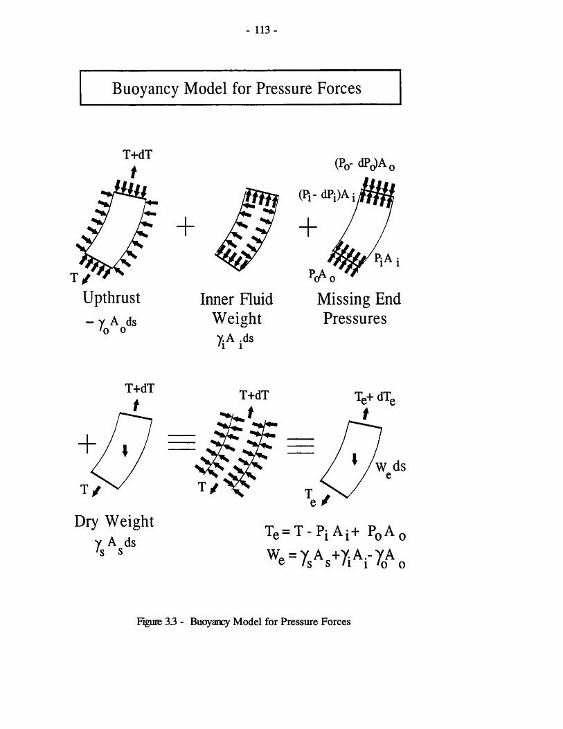
- 113 -

Buoyancy M odel for Pressure Forces

Upthrust- y A ds 'o o

+Inner Fluid

W eighty.A .ds n i

(Po- dPo>A0

M issing End Pressures

T+dT T+dT

Dry W eight Y A ds/ c S

Te+ dTe

W ds

e

T - P; A ;+ A

We = Y A +Y A.- YA 6 /s s »i i »o o

Figure 3.3 - Buoyancy Model for Pressure Forces

- 114 -

Curved Pipe Element for Exact Analysis

dA

O

figure 3.4 - Curved Pipe Element for Exact Analysis

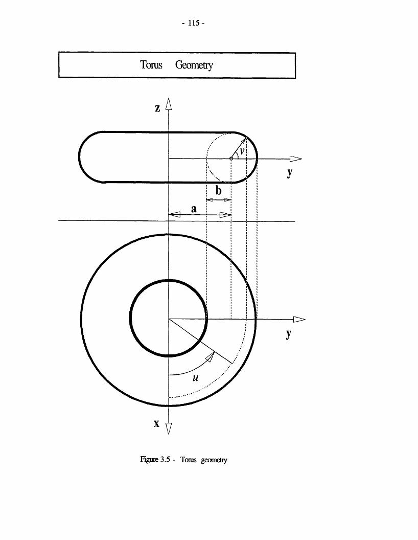
- 115 -

Tonis Geometry

Figure 3.5 - Torus geometry

- 116 -

Local Torus Co-ordinate System in Three Dimensions

y’— c

z

Figure 3.6 - Local Torus Co-ordinate System in Three Dimensions

- 117 -

Forces on a Curved Pipe Section

T+dT. M+dM

0+de

V+dV

/ - OZ

/'

Figure 3.7 - Forces on a Curved Pipe Section

-118-

CHAPTER 4 : ANALYTICAL SOLUTIONS

4.1 - INTRODUCTION

Major pipeline and riser designs for offshore applications rely on computer simulations of one form or other. However, data preparation and computer time requirements of these methods often impose constraints on the time and cost schedule of most projects. Since the major objective of a preliminary study of a suspended pipe system is one of determining the most suitable geometry for the given application, an iterative procedure involving numerous computer runs is often unavoidable. Structural parameters comprise horizontal and vertical separations, total pipe length, position of the mid-water arch, expected vessel motions, bend radius restrictions, internal flow, fatigue life and wear criteria. In addition, the total number of lines, cost restrictions, fabrication schedules, transportation and installation method form the non-structural parameters. Simultaneous satisfaction of all these constraints is currently impossible, leaving a step-wise procedure the only alternative.

The shape of a suspended pipe is governed by the catenary equations. These represent a class of equations which take different forms depending on the geometric boundary conditions of the system. Solution of these equations provides the pipe profile and its tensile, shear and bending stress distributions under a uniform self-weight. Hence, only vertical loads of uniform distribution along the arc-length may be accommodated. Nevertheless, in the absence of localised weight or buoyancy attachments, self-weight is the main contributor to the pipe shape. Several design variables may be investigated using simple catenary analyses. These include separation, buoyancy requirements at the mid-water arch and vessel motions (in a quasi-static sense). In this chapter a number of common configurations are studied. Solutions are presented in closed form- where possible- or in the form of systems of simultaneous equations requiring simple iterative solutions. The advantages of these techniques lie in their simplicity and speed which allow a large number of configurations to be studied in a time less than that required for

-119-

a single computer simulation. For cases where the pipe is sufficiently taut to be approximated by a straight line, considerable simplifications result. In selected cases, good estimates of the natural frequencies of the structure and its dynamic response are shown to be possible.

This chapter starts with a derivation of the elastic catenary equations including the effects of axial elongation. A series of specialised applications are then studied. Initially, the simple catenary profile is studied which is directly relevant to pipelaying and mooring line calculations. The assumption of zero seabed angle and axial inextensibility of the pipe are then introduced and it is shown that for such cases, closed form solutions are possible.

Progressing further, the more elaborate cases of the steep-S and the lazy-S risers are studied; both of which include a tethered buoy. The equations of equilibrium of the tethered buoy are used to show that these are linearly dependent on the horizontal and vertical forces resulting from the suspended weights of pipes to its either side. For a given set of catenary forces, the net residual force at the buoy is shown to be directly available. Hence, using a general algorithm for solution of the standard catenary equations, an iterative method is employed for solution of the equations concerned. The simple catenary algorithm presented by Peyrot and Goulois(1978) has been used in this work.

The steep-S profile calculation is started from a vertical buoy position. The buoy is then allowed to translate laterally under the action of the force residual until equilibrium is achieved. The displacements of the buoy depend on the tether stiffness in lateraltranslation. Special features have been incorporated into the abovealgorithm to enable accurate fitting of the catenary pipe to the

| surface of the buoy. This feature is of special importance if theresulting profiles are used in generating a finite element mesh as it offer the required continuity of the pipe curve. The suggested

j algorithm is used in Chapter 8 for a study of the sensitivity of| the configuration to vessel motions in surge and heave in afi quasi-static sense.

-120-

The static equilibrium of the lazy-S profile is obtained by assuming that in the absence of exciting forces other that self-weight, the tether remains vertical. This is an intended feature in all designs of these risers as a vertical tether provides the greatest support and lateral stability. For a given length of pipe on the vessel side, a unique solution for the lower simple catenary exists which provides a horizontal tension at the buoy interface identically equal to that due to the opposite section of catenary. This may be determined from the pipelaying equations in closed form. An additional length of pipe must be allowed to rest on the seabed to accommodate pipe lift-off caused by buoy excursion under environmental loads and vessel motions. It then remains to iteratively fit the pipe angle to the buoy surface at either end and check the reduction in tether tensile forces due to the vertical pipe weights it is required to support. Having established the equilibrium position, quasi-static analysis of the riser geometry under vessel motions may be carried out using a similar procedure to the steep-S case but with some extra complexity. This arises from the ability of the lower pipe for lifting off and laying down on the seabed. This constitutes a non-linearity which is easily accommodated using the algorithm used for pipelaying analysis.

The steep-wave geometry is a modification of the steep-S variety where the tethered buoy is disposed of altogether and replaced by a section of buoyancy collar. The governing equations for the steep-wave risers are significantly different from those of steep-S risers. Instead of the equations of force equilibrium, those of horizontal and vertical geometric compatibility must now be considered. These comprise a set of three simultaneous non-linear equations, one for each segment of pipe; namely, the lower catenary, the intermediate buoyancy collar and the upper sagging portion. It is shown that it is possible to develop a set of general equations for catenaries composed of multiple pipe sections. These equations are further illustrated to remain dependent on two variables, irrespective of the number of sections involved. Similar equations are developed for lazy-wave risers with the only difference being that the variable seabed length replaces

-121-

the pipe angle at the seabed as a variable; the seabed touch-down angle being invariably zero in all cases by definition. These equations are, similarly, shown to be applicable to multiplesegmented risers.

The last heading in this chapter examines the very specialised andlimiting case of towed pipelines. These fall at the limit where thecatenary equations revert to the simpler parabolic cable equations. This transformation arises as a result of the very small sag to span ratios of these pipes which permits their weight per unit length to be considered uniform along the horizontal axis instead of the arclength. Towing methods are a relatively new means for transportation of long lengths of pre-fabricated pipelines to an offshore site. Their use was first considered as a cheapalternative to traditional pipelaying procedures which are sensitive to weather conditions which could halt the supply of pipe sections to the laying vessel. In towing operations, the pipe is fabricated onshore, all personnel costs are reduced, and relatively inexpensive and unsophisticated tow vessels are used for transportation to the offshore site. However, the major disadvantage of towing methods lies in the high risks involved with exposing a much larger and more expensive section of pipe to operational hazards. The last heading in this chapter describes the development of simplified static and dynamic analysis algorithms for towed pipelines. The latter carried out in the frequency domain using a distributed parameter modal analysis. The numerical analysis of the dynamics of towed pipelines is usually very time consuming. This is a result of their large dimensions compared to typical wavelengths which necessitates the use of a very large number of finite elements. The proposed methods are shown to provide a very fast calculation method. It is shown that, using these techniques, results of sufficient accuracy for preliminary design may be obtained at greatly reduced time and effort.

-122-

4.2 - ELASTIC CATENARY EQUATIONS

In the absence of fluid drag and pressure forces and after division by (ds), Equation (3.6.9) becomes,

T !r - ;r - w cosS ~ 0ds dS (4.2.1)•. d 0 , -where ^ is the exact expression for curvature.

The equation for the shear force and bending moment along the beam given by (3.6.13) and (3.6.15) are now used to give,

T ^ — EI — w cos 0 - 0dS dS (4.2.2)

Equilibrium of horizontal forces between points 0 and A in Figure(4.1) yields,

H0 — T cos0 + V sin0(4.2.3)

Substituting for V and re-arranging, we have,

d 2 0T = H0 s e e d — EI tan#

Substituting this equation into (4.2.2) gives,

H0 sec# rjp- — EI | tan “ T T — w cos ™ 0 0 ds ds2 ds ds3

or more concisely,

(4.2.4)

(4.2.5)

EI [ sec* if* 1 - H» sec2$ i f + ” " 0as as as (4.2.6)

which is the equation of equilibrium for a uniform beam under self-weight and includes flexural effets. If the flexural rigidity term (EI) in equation (4.2.6) is ignored, we have,

-123-

2 a Wsec20 — - — ds H0(4.2.7)

which can be simplified to,

h < tan* > - k(4.2.8)

Integrating between limits ( 0 — ► s ) gives,

wstan0 - — + tan0o Ho(4.2.9)

where 6 0 represents the angle at the base of the pipe. The equationof equilibrium becomes,

T — — w cos6 ds (4.2.10)substituting for ~ from (4.2.7) gives,

T (s) — H0 sec0(4.2.11)

Using (4.2.9) and the identity (sec2 i> — 1 + tan2^) , we get,

T (s) - H0 [ 1 + ( + tan0o)2 ]l/2n0(4.2.12)

for small axial strains e, the stretched length is given by,

«s0 - ( 1 + e ) «S - ( 1 + L ) {s(4.2.13)

where subscript s0 refers to the stretched length of the element, for small s0 , the projections of the element on the axes are,

6x « 6s0 cos#(4.2.14)

6y - 6s0 sin0(4.2.15)

Substituting for 6s from (4.2.13) and taking the limit as s — ► 0,

-124-

dx r - , WS - T -1/2 Hfai " f 1 + ( s; + tan*o> ] + EA

(4.2.16)

x (s) “ ^ [ sinh" ( — + tan0o) - sinh’ ( tan0o) ] +(4.2.17)

Similarly,

g - ( ^ + tan*0) [ [ 1 + ( ^ + tan*0)2f l/%- S* ](4.2.18)

y(s) - ^ [ [ ! + ( ^ + tan#0)2] ^ - ( 1 + tan28 0 ) ^ ]

ws2 sHf 2EA EA+ xttt + ~. Q tan0o

(4.2.19)

Now, using (4.2.13) we have,

“ "••>■ i v '(4.2.20)

which after integration gives,

Hrt ® r . i \j s - is0(s) - s + 2 L sinh + tan^o) - sinh (tan00) +

ws ws /2 i/2 _(— + tan0o)[ 1 + (— + tan00) ] / ~ tan0o[ 1 + tan20o] / ](4.2.21)

To obtain expressions for shear force and bending moment, expressions for curvature and its first derivative are required. These are given by,

w r i , / w s . a \ 2 I"1/2di - r0 I-1 + <s;+ tan6 21(4.2.22)

0 - -2 ^ <i£ + tan*°>[1 + <■¥, + tan‘°)2 r *(4.2.23)

At given arclength, the angle of the pipe from the x-axis is,

-125-

- ws 0 (s) - tan ( — + tanfl0)Ho(4.2.24)

Comparison of Equation (4.2.10) with (3.6.9) shows that, in the absence of current loading and neglecting flexural effects, these are identical in form. Further, it is readily seen that using,

T - T + P A - P.A. - p.U? A. eff o o l i ri l l

w = 7 A + 7.A. — 7 A eff 's s l i 'o o(4.2.25)

(4.2.26)

to replace T and w, it is possible to use all the equations derived in this section for calculation of the profile of a flexible riser subjected to self-weight, internal and external pressure forces and a steady internal flow. These considerations significantly simplify the computation of the static profile of a flexible riser and avoid lengthy numerical procedures. andWeff are usually referred to as the "effective tension" and "effective weight" of the pipe.

Once the pipe geometry has been defined, T, which represents the physical tension in the wall of the pipe may be derived by subtraction of other terms. An interesting observation is that according to the formulation for effective tension, changes in internal and external pressures and densities or internal fluid velocity will not affect the pipe geometry but merely alter its wall tension distribution. Further, it should be noted that the pipe geometry or its stress state are independent of the internal flow direction.

4.3 - PIPE-LAYING EQUATIONS

A pipe-laying profile refers to the simplest catenary configuration where the top end of the pipe is fixed and the bottom end is at rest against a horizontal boundary. Such situations arise during laying of offshore pipes, mooring of vessels and guyed towers and with some variety of flexible riser applications. Since the same equations govern the behaviour of all these systems- and for simplicity- these are considered under the common heading of

-126-

pipe-laying equations. These equations are obtained through substitution of a fixed seabed angle into the elastic catenary equations developed earlier. Two modifications are introduced at this stage. Firstly, the effects of axial elongations are ignored- this is permitted due to its small magnitude in all cases of practical interest. Secondly, it will be assumed, hereafter, that the seabed slope is zero. This simplification is justified since seabed plains have typical slopes of the order of 5 degree with higher slopes restricted to hilly regions. For pipelaying conditions, designers tend to avoid these areas as much as possible; failing this, more detailed account of the topography is taken and detailed analyses are carried out which allow for effects such as axial and lateral friction which are of importance for such conditions. In most cases, the use of catenary equations for such situations is not justified. Based on these arguments the assumption of zero seabed slope may be defended as being one of greatest practical interest.

For a zero seabed slope (5-0), Equation (4.2.17) simplifies to,

/ \ H0 . , -1/wsN x (s) - sinh (— )w n o

(4.3.1)

which gives,

s(x) - sinh (JP)w H0(4.3.2)

Substituting this into Equation (4.2.19) and simplifying yields,

y(s) = [ cosh(jp) - 1 ](4.3.3)

Squaring Equations (4.3.2) and (4.3.3) and subtracting the former from the latter and reducing, we get,

-127-

H0 _ s2—y2 w 2y (4.3.4)

For completeness, it is noted that for a non-zero seabed slope, the above expression becomes,

M o _________ s2-y2_________w 2(y see#,— s tan0, )

(4.3.5)

These expressions are of use in determining the top tension requirements in terms of the water depth and suspended pipe length. Equation (4.3.5) is equally applicable to flexible riser cases where the base angle is known. In pipeline design, the horizontal vessel pull is restricted by the vessel power and usually assigned a maximum which is within a safe margin of the maximum vessel capacity. Situations also arise where a damaged section of the pipe needs to be retrieved and replaced or other cases arise where adverse weather conditions force the operator to halt laying and lower the pipe end onto the seabed. The above two cases are normally referred to as pipeline pick-up and lay-down. Both these operations requires the suspended length of the pipe to bedetermined. Equation (4.3.4) provides this on re-arrangement. The criterion during lay-down and pick-up is that the bending stress or equivalently the curvature at the seabed is kept constant. Equation(4.2.22) shows that this implies a constant H0. For example, in the case of pipeline lay-down, having capped the pipe end on thevessel, a cable is attached to this section which is paid out keeping a constant horizontal tension. This corresponds to the design tension for laying the pipe. The vessel movements should clearly duplicate the reverse of those used in laying.Additionally, the total length of cable is equal to the suspended length of pipe given by Equation (4.2.19) which provides,

H0 y cos w 1 — cos 8

(4.3.6)

This form of the equation is the most suitable for pipelaying as it allows the determination of all variables in terms of quantities at

the vessel attachment point. In a typical situation, the water depth is known and the required vessel pull is a constant design parameter which allows the required stinger angle to be determined from Equation (4.3.6). This may equally be determined from Equation (4.2.24).

Flexible risers of simple catenary configuration may be analysed directly using the pipelaying equations presented so far in this chapter. The main difference between the application of these equations to pipelaying and flexible risers is in the choice of variables involved. With pipelaying problems, the designer is usually concerned with variables at the vessel end; namely, the pipe slope and the horizontal tension (vessel thrust)- conditions which are fully defined analytically. In contrast, flexible riser problems involve the use of three geometric compatibility variables which are the vertical and horizontal offsets and the total pipe length. Whilst the nature of the problem remains the same, its formulation and hence solution are altered significantly. The problem is now one of determining the length of pipe resting on the seabed. The seabed is assumed to be of constant slope 6 the pipe of total length, s, which is the sum of the length resting on the seabed, s^, and the free length, s^. As illustrated earlier, for a given seabed slope, the pipe shape is a function of water depth only. This is because the imposition of a constant 6^ removes one of the variables required in solution. The horizontal top tension is easily determined using Equation (4.3.5) and allows the computation of the total horizontal offset generated. This may then be compared to the required value and s^ altered until the total generated offset is within the required tolerance of the given value. The mathematical statement of geometric compatibility may then be written as the following system of simultaneous equations,

-129-

(4.3.8)H0 s| - ( y - sbsin b)2w 2 ( y sec0, — s-tanfl, )

(4.3.9)

Note that Equation (4.3.9) is an alternative representation ofvertical geometric compatibility. Although the above equations maybe reduced into one by substitution, the resulting expression does not have a closed form solution and must be solved iteratively. The iteration is exceedingly simple and requires incremental increases of sb until Equation (4.3.7) changes in sign to indicated that the solution has been overshot. Starting with the quantities from the previous step, sb is now incremented in smaller steps and the procedure repeated until convergence.

4.4 - STEEP-S RISERS

A steep-S riser configuration denotes a riser geometry composed of a lower vertical pipe section which at some depth climbs over a subsea buoy and continues to the vessel describing a sagging upper part. The basic geometry is shown in Figure (4.3); although other variations are also possible. One such variety is produced where the buoy is tethered for additional lateral stability. Where the tether forms a structural part of the system, it helps reduce the tensions in the lower vertical pipe. The governing equations remain the same except for a change in the lower equilibrating force.Another variety disposes with the buoy and tether arrangementaltogether and replaces the former with a collar of buoyancymaterial. This configuration is referred to as the steep-wave profile and is studied later in this chapter. The staticequilibrium of the buoy in Figure (4.3) requires that the resultant of vertical and horizontal forces on the buoy reduces to zero. For the given geometry, the equilibrium of horizontal forces yields,

-130-

H ~ T- sin0 - 0(4.4.1)

where refers to the tensile force at the top of the tether. Note that at the seabed, the tensile force becomes T0 (=T^—wl) to allow for the weight of the suspended pipe. Vertical force equilibrium gives,

F, - V - T- c o s O - 0(4.4.2)

The inclination of the tether to the vertical is,

-1 H< f ~ v >

b (4.4.3)

For a given separation (x,y) between the buoy and the vessel and a constant length s, calculation of H and V requires the solution of the catenary equations using an iterative procedure. This solution algorithm must be combined with the algorithm for the overall equilibrium equations which must also be solved iteratively. The flow-chart for the system equilibrium calculations is given in Figure (4.4). A typical algorithm for solution of the catenary equations is given by Peyrot(1978) and may be used here. The flow-chart includes an adjustment of the slopes at the buoy interface to avoid a discontinuity. The slope at the base of the sagging part is a function of (x,y,s). Consequently, with increasing x separation, the riser will lift off the buoy unless constrained against such movements. For all cases of engineering interest, constraints at this location should be avoided as they give rise to high localised bending moments and continual wear of the pipe. One is, therefore, justified in assuming that the pipe is free to adjust its slope to match that of the buoy surface.

It must be noted that solution of the overall equilibrium equations for steep-S riser geometries may equally be attempted using Equations like (4.2.17) and (4.2.19) directly in the overall system equations. However, the use of such a method would require

-131-

the use of a general purpose mathematical algorithm for solution of systems of simultaneous non-linear equations. The suggested alternative offers greater simplicity and relies on the use of a standard algorithm for solution of the catenary equations, examples of which are widely available.

4.5 - LAZY-S RISERS

Lazy-S risers are a modified form of the steep-S variety where the lower section of the riser, instead of being vertical, forms a simple catenary to the bed. Lazy-S risers are used where the horizontal offset between the vessel and the well-head is too large to be accommodated by steep-S type risers. A lazy-S riser is schematically illustrated in Figure (4.5). The equations of horizontal equilibrium at the buoy may be written as,

Hx — H2 + T, sin# - 0(4.5.1)

where Hj and H2 are the horizontal components of riser tension at the buoy and T^ is the tether tension at the top. Using the equations for vertical equilibrium we have,

F - T.. cos# - Vj - V2 - 0(4.5.2)

where V! and V2 refer to the vertical component of tension due to adjacent riser parts. The tether inclination may then be calculated by combining the above equations to give,

i H,- H2tan ( Fb- V ! - V 2

(4.5.3)

Hj , H2 , Vj and V2 must all be determined from the solution of the catenary equations to either side of the buoy. The global equilibrium is determined iteratively: First, starting values ofvariables are determined for zero tether inclination. The equilibrium of forces at the buoy is checked and the required tether movement to balance this force calculated. For the new buoy

-132-

position, the equilibrium is checked again and the procedurerepeated until convergence is established. The flow-chart for thisprocedure is illustrated in Figure (4.6) which includes aprovision for adjustment of the pipe angles at its interfaces withthe buoy surface.

4.6 - STEEP-WAVE RISERS

Steep-wave riser are composed of a taut lower pipe connected to a positively buoyant section of catenary which itself joins the sagging part of the riser which in turn ends at the vessel. This geometry is shown in Figure (4.7) and is seen to be a more complex version of the steep-S geometry where the buoy arch is replaced by a free catenary. The equilibrium position for this geometry may be calculated using the equations of geometry. The equation of horizontal compatibility for a riser composed of (n) sections of different effective weights may be written as,

S -x.± - X - 0i"1,n (4.6.1)

and in the vertical direction,

2 y. - Y. i J l1=1 ,n (4.6.2)

(4.6.3)

(4.6.4)

where,

H -i w is i -ix. = —0 [ sinh ( — — + tan*.) — sinh (tan*.) ] l w. rln l ll 0

. . W . S . n I Mtj 1 JO

y. = -o [ [ 1+ ( + tan*.) ] / - [ 1 + tan2*.] / ]w. 1 L Hn l 1 1 iJ Jl °

B i + X - tan-' ( -|-i + tan^ )(4.6.5)

where (n=3) for the pipe shown in Figure (4.7). The focal consideration is the constancy of H0 which is merely a statement of horizontal equilibrium. This arises from the lack of all external horizontal force resultants. It is noted that these equations may

-133-

be expressed in terms of the two variables H0 and 0 lf all other quantities being related. An iterative procedure is required for solution of this class of equations. Many standard mathematical algorithms are available for this purpose. For this work, the NAG (Nottingham Algorithms Group) routine C05NBF was utilised.

4.7 - LAZY-WAVE RISERS

Lazy-wave risers are typically comprised of four sections. A free length is provided on the seabed which rises in a simple catenary profile to the mid-water arch which forms a positively buoyant catenary section and which, in turn, joins the sagging part of the riser terminating at the surface vessel connection. This geometry is illustrated in Figure (4.8). The equation of horizontal geometric closure for a catenary composed of (n) consecutive sections takes the form,

s. . + S x. - X - 0bed . - li-1’n (4.7.1)

and vertical geometric closure condition leads to the equation,

S y. - Y - 0 i-l.n1

where,

2 W . S 2x. = —0 [ sinh ( „ + tan0.) — sinh (tan0.) ]l w. Hn l l Jl 0

y. - -o [ [ i+ ( -jjj-1 + tan0. ) V /2- [ 1 + tan20.]1/2] J i w. 1 Hft l 1 1 iJ Jl 0

'i+i= tan_1 ( ~ k r + tan9i )

(4.7.2)

(4.7.3)

(4.7.4)

(4.7.5)

subject to the boundary condition 0^-0. Since all the loads acting on the system are vertical, the horizontal force equilibrium implies that H0 remains constant throughout the length of the pipe which allows the expression of all the above equations in terms of

-134-

Sj and H0 only. Due to the non-linearity of these equations, a standard mathematical procedure must be employed. For the purpose of this work, the NAG algorithm C05NBF which was also used in the solution of the steep-S problem was utilised.

-135-

4.8 - TOWED PIPELINES

Transportation of pre-fabricated pipelines or tethers by towing offers a cheap and time saving installation method. Calculation of the static and dynamic response of towed pipelines is conventionally done using a finite element or equivalent numerical analysis technique - see Redshaw and Stalker(1976) or Rooduyn and Boonstra(1985). Similar work has been done on towed instrument arrays used in offshore surveying - see Kato et al.(1985). The typical geometry of a towed pipeline allows simplifications to be introduced and solutions obtained using analytical rather than numerical techniques.

A typical towed pipeline may be from 0.5 to 4 km in length but only 1 to 2 metres in diameter. This justifies the assumption of negligible bending stiffness for a preliminary static design. The case of a pipeline with a small sag to span ratio and without attachments is governed by the conventional catenary equations. The addition of chains and buoyancy modules tends to distort the natural catenary shape but provided the distribution of these is relatively uniform along the pipe and they appear in a sufficiently large number, the catenary shape will be closely approximated. Furthermore, since these lines typically have very small sag to span ratios, the assumption of uniform weight along the arclength may be replaced by one of uniform weight along the horizontal axis. This approach allows the parabolic cable equations to replace the catenary equations; considerably simplifying the algebra. For the geometry in Figure (4.9a), the parabolic cable equations - see Meriam(1980)- define the pipe slope as,

dy wxdx H0

(4.8.1)

where w is the net buoyant weight per unit length of the pipe bundle including the effect of mass or buoyancy attachments distributed as equivalent uniform loads and H0 is the horizontal end tension. Integration of this equation yields the equation of shape,

-136-

wx2y " 25;

(4.8.2)

By evaluating this at x - L/2 and equating with the central sag, h, we also obtain,

Figure (4.10) illustrates the level of approximation involved in using the parabolic cable equations in place of the catenary equations for pipes of small sag to span ratio. It is noted that with reducing sag the catenary equations become almost indistinguishable from the parabolic cable equations.

Considering the free body diagram of an element of pipe, the vectorial summation of forces yields,

w 8h H0 “ L2

(4.8.3)4hx2

(4.8.4)

T =* ( H2 + w2 x2 ) '(4.8.5)

and upon substitution for H0,

(4.8.6)

The maximum tension occurs at x — L/2. Thus,

T wL max 2 (4.8.7)

The length, s, of the pipe is found by integration,

-137-

(4.8.8)

which gives,

(4.8.9)

With the geometry of the pipe fully defined, it is possible to examine the effect of loading due to in plane current whose velocity is assumed constant with depth for simplicity. Consider the vertical equilibrium of forces in Figure (4.9b) noting that the co-ordinate axes have been shifted to the pipe end.

(4.8.10)

where,

V0(x) =- w ( x - | )(4.8.11)

and for horizontal equilibrium,

F dxx(4.8.12)

For moment equilibrium,

M(x) - M0- T(x).y - V(x).x -J0

.xF .x dx —y F .y dx x J

(4.8.13)

with the notations of Figure (4.9b). Using the normal component of fluid velocity, the drag force components per unit length on an element of pipe immersed in a current flowing in the positive x

-138-

direction is given by,

F - ~ P C , R U2 sin30 dxx r o d o for 0 < x < £(4.8.14)

F - + p CJ R U2 sin35 dxx o d o (4.8.15)

and,

F - + p C , R U2 sin20 cos 9 dx for 0 < x < ^y ° d ° 2 (4.8.16)

F - — p C, R U2 sin20 cos 6 dx for 7? < x < Lv o d o 2y (4.8.17)

Note that the origin of co-ordinates has been shifted to (L/2,h).

The sine and cosine functions in Equations (4.8.14) to (4.8.17) above can be conveniently represented as functions of pipe slope using (3.6.11) and (3.6.12) and substituted in equations(4.8.10), (4.8.12) and (4.8.13) to yield expressions forhorizontal tension, vertical shear and bending movement along the pipe. A simple transformation of co-ordinates will then yield the force resultants along the axis of the pipe.

DYNAMIC ANALYSIS

Dynamic response of the pipeline in regular waves can be calculated using a modal decomposition method. The bundle is idealised as a distributed parameter system with lumped masses and srings at its ends - see Figure (|C.9a). Details of the method may be found in Clough and Penzien(1982) or Thomson(1981). First, an eigen-valve analysis is carried out to obtain the natural frequencies of the pipe. A Rayleigh-Ritz formulation offers a particularly simple and accurate method for such calculations. The potential energy of the system is expressed as a summation of the strain energies in flexure, translation and rotation of the end springs and the axial elongation of the pipe. The kinetic energies are due to the inertia

-139-

of the distributed pipe mass and the lumped masses at the ends of the pipe. The total energy is the sum of the potential and kinetic energies and is stated by,

n U + T + 2 U. + S T.1 1 1 1 (4.8.18)

n fJo

El y"(x)2dx + 2 ky Xj-0,L

+ 75- k y' (x. , t)2 r J 1 i rL:i_ °-L 2 Jo

T(x) y'(x)2dx

| J m(x) y(x,t)2dx + | M y(xift)(4.8.19)

where the (') and (.) denote differentation with respect to x and t respectively, k^ and k^ are the vertical and rotational end spring stiffnesses, m(x) is the combined mass and added mass per unit length of the pipe and M is the lumped end mass.Minimisation of the total energy of the pipe is represented by,

^ - dU + dT - ° (4.8.20)

The Rayleigh-Ritz method requires an estimate of the deflected shape which at least satisfies the geometric boundary conditions of the system. The accuracy of the resulting eigen-valve analysis depends on how closely the estimated profile resembles the actual deflected shape. Since a large number of modes are usually used in dynamic analysis of towed pipelines, and to maximise accuracy, a Fourier series is chosen to represent the deflected shape. The series expansion takes the form,

__ r . . ,n7rx. „ ,n7rx. 1 iwty(x,t)= S An sin (— ) + Bn cos (— ) J e

for n - 1,2,3,...(4.8.21)

-140-

The sine terms represent the anti-symmetric vibration modes whilst the cosine terms represent the symmetric modes. and areconstants determined from boundary conditions. It is noted that the cosine terms are included to account for the displacements in the springs at the pipe ends. Substituting equation (4.8.21) into(4.8.19), minimising the resulting expressions with respect to modal constants A^, and using modal orthogonality relations - see Clough and Penzien(1982) - the eigen-value problem is conveniently decomposed into two uncoupled symmetric and anti-symmetric problems. From the solution of the minimised equations, The eigen values for the anti-symmetric modes are givenby,

<f>* [ ^ ( ^ > 2 + 2kr + I| ]w2 _n .mL.C2 * (4.8.22)

and those for the symmetric modes by,

[ 5 S (IS) 4 + 2y (B £ )S t l j(J)4n 2M )

(4.8.23)

Before progressing with the modal analysis, boundary conditions are used to establish the required coupling between symmetric and antisymmetric modes of vibration. Using the standard equation for shear force,

V - El y'" (4.8.24)

the equilibrium of vertical forces for each mode at x = 0 can be written as,

El y‘ x-0 x=0 — M y x-0 (4.8.25)

-141-

Similarly equilibrium of rotations for each mode at x - 0 gives,

El y'' x-0 k . y'r J x-0 (4.8.26)

Substituting for y from (4.8.21) into (4.8.25) and simplifying gives,

B - (^)3 Eln L.A k + M u)2n 7 n (4.8.27)

Similarly, for the anti-symmetric modes of vibration,

B - (^) El n LA kn r (4.8.28)

Using equation (4.8.27) and (4.8.28), we can now write the mode shapes as,

/ iwt ^ a T 4 ,n7rxN Bn .njrx.ly(x, t)- qe S An sin + cosn (4.8.29)

It is noted that with increasing stiffness of the vertical spring in Equation (4.8.27), the ratio (B^/A^) tends to zero, thereby eliminating the symmetric modes of vibration.

The equation of dynamic equilibrium takes the usual form,

m y + b y + El y " " - f(x,t) (4.8.30)

where f(x,t) represents the forcing function and b is the total damping constant. The solution is of the form,

-142-

y(x,t) - S <f> (x) q (t)(4.8.31)

where <f>n is the shape of mode n and q^ is a time dependent constant. Using equation (4.8.29), we can write,

B, , . ,n7rxN . n ,n7rxN^n (x) - sin (— ) + -— cos (“l")n (4.8.32)

Substituting equation (4.8.32) into (4.8.30), premultiplying by <f>s and integrating gives,

m c 2(^ q ) dx s n n n

El <f> ' " q ) dx -s n n n <f>s f (x, t)dx(4.8.33)

Using the modal orthogonality relationships,

 m 6 dx - 0 s n(4.8.34)

<f> El <f>' ' " dx - 0 , n -/- ss n(4.8.35)

and,

<f> El <f>' ’ "dx n n u>4n m [ <f> ]2 dx 1 n J(4.8.36)

we get,

-143-

q + — q + o>z an m n n n m$n^n (x) p(x,t) dx

(4.8.37)

where,

$n [<t>n ] 2 dx(4.8.38)

Since the forcing function is harmonic, the response will also be harmonic and we may write,

/ - \ “ lwt q (t) - q en n (4.8.39)

where q^ is the modal participation parameter in mode n. Substituting (4.8.22) into (4.8.20) and simplifying we get,

( —gj2+ iw — + u>2) q — ——m n ti m$n^x ) p(x, t)dx

(4.8.40)

and,

<£n (x) p(x, t) dx

nm$ (a>2 — w2) + iw — n n m J

(4.8.41)

Since the eigen-values for the symmetric and anti-symmetric modes are different, is used to denote the anti-symmetric modes and

the symmetric modes. We have,

=n m$

|*L . .nTrx. . \ jQ s m (-£“) p(x,t) dx

T(w2 — w2) + iw — 1 A |"(w [ An m J n [

B n J o+ -----L . n?rx. . . v .cos (—— ) p(x,t) dx

2 — w2) + iw — 1Bn ' m J(4.8.42)

-144-

Suinming the responses over the required number of modes yields the total deflection. This also permits the internal forces to be determined.

The dynamic wave force per unit length of an element of pipe is given by the Morison equation (6.2.5) where the fluid velocities are obtained from the Linear (Airy) wave theory,

f(x,t) - p A C u - p A (C -l) x + p C R o o m n o o m n o a o u — x n n (u - x )n n (4.8.43)

The vertical fluid velocity, using the notations in section (6.3), is given by,

sinh k(y+d) .. .u o> r\ cos (kx-wt)n sinh (kd) (4.8.44)

and vertical fluid acceleration by,

u - — w2rj ~S'%nr cos (^x-wt)sinh (kd) (4.8.45)

A possible simplification may be introduced by ignoring the effects of structural displacements in the linearised drag coefficients and using the absolute value of fluid velocities. Having combined the added mass term with the physical mass term on the left hand side of the equations of motion, the hydrodynamic loading becomes,

of(x,t) = p A C u + — p C.Ro o m n 3ir o d o umax .(u - x ) n n

(4.8.46)

The linearisation technique is that due to Krolikowski and Gay(1980) and is described later in section (6.4) of this thesis. The last term represents the equivalent drag damping and can be similarly combined with the structural damping term on the left hand side of the equations of motion. The pipe also offers structural damping which can be quantified by assuming a Rayleigh type mass and stiffness proportional damping - see

-145-

Clough and Penzien(1982) - given by,

b - a m + /3 ElS (4.8.47)

where constants a and f} are estimated or determined using the results of the eigen-value analysis. Finally, the drag force induced damping is given in linearised form by,

gb , ■* q p C, Rd 3?r o d o umax

(4.8.48)

The simplifications introduced allow Equation (4.8.42) to be integrated analytically. Although the computations are relatively long, a consideration of the relative magnitudes of the modal participation parameters, will normally permit a large number of higher modes to be excluded from analysis, hence reducing the number of calculations. It should be noted that although the results of such dynamic analyses may not be of required accuracy in design, the use of this simple method allows a suitable preliminary indication of pipe geometry, tensile, shear and bending forces, natural frequencies and dynamic response characteristics. Further, as with this class of problem a large number of modes are expected to contribute to the overall response, a large number of natural frequencies must be determined. Although this requires little effort with this method, it is nevertheless a large computational exercise with numerical finite element methods where an eigen-value analysis must be carried out whose cost increases rapidly with increasing number of required eigen-values. Since the minimum required number of modes may not be anticipated before the analysis, usually a larger than necessary number of modes must be used. The foregoing method allows a good estimate of the modal participation parameters with great speed which may be used as a guideline before finite element runs. Additionally, a prior knowledge of these parameters helps proportion the element sizes, a factor which is also of great importance in accurate finite element modelling.

- 146-

Elastic Catenary Model

0(S) \ M(s)

T + dT

a / e + c m M + dM

V + dV

Figure 4.1 - Elastic Catenary Model

- 147 -

Simple Catenary Riser M odel

o

Figure 4.2 - Simple Catenary Riser Model

- 148 -

Steep-S Riser Geometry

v v

/ | - ^

figure 4.3 - Steep-S Riser Geometry

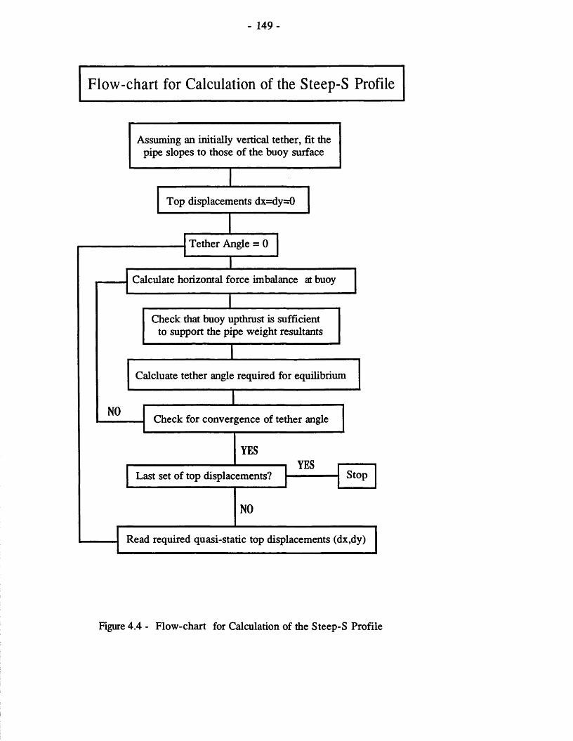
- 149-

YESYES

Stop

Tether Angle = 0

Last set of top displacements?

Top displacements dx=dy=0

Check for convergence of tether angle

Calculate horizontal force imbalance at buoy

Check that buoy upthrust is sufficient to support the pipe weight resultants

Read required quasi-static top displacements (dx,dy)

Calcluate tether angle required for equilibrium

Assuming an initially vertical tether, fit the pipe slopes to those of the buoy surface

Flow-chart for Calculation of the Steep-S Profile

Figure 4.4 - Flow-chart for Calculation of the Steep-S Profile

- 150-

Lazy-S Riser Geometry

o

0/ Vi+ \£

I E3»

Figure 4.5 - Lazy-S Riser Geometry

- 151 -

NO

YES

Stop

Tether Angle = 0

Check for convergence of tether angle

Read required top displacements (dx,dy)

Calculate horizontal force imbalance at the buoy

Calculate tether angle from vertical required for equilibrium

Fit the pipe slopes on either side of the buoy to match those of the buoy surface at contact point

Flow-chart for Calculation of the Lazy-S Profile

Assuming a zero tether angle for the at-rest profile, calculate the horizontal force resultant at the buoy due to the weight of the sagging part of the riser. Proportion a lower catenary which produces a force equal but opposite to the above

Figure 4.6 - Flow-chart for Calculation of the Lazy-S Profile

- 152-

Steep-Wave Riser Geometry

Figure 4.7 - Steep-Wave Riser Geometry

- 153 -

Lazy-Wave Riser Geometry

H ----- Cs>fe— ■ c H -O '

1 x2K

Figure 4.8 - Lazy-Wave Riser Geometry

- 154-

Towed Pipeline M odel

(a)

V(x)A Fy

o Fx

(b)

Figure 4.9 - Towed Pipeline Model

- 155 -

0.0 -i

-0.1

-0.2 -

^ -0.3 -

-0.4 -

-0.5 -

-0.6-0.50 -0.25 0.500.00 0.25

x/L

- LEGEND - Catenary

Parabolic

Figure 4.10 - Comparison of catenary and parabolic profiles for different

pipe lengths

-156-

CHAPTER 5 : FINITE ELEMENT STATIC ANALYSIS

5.1 - INTRODUCTION

The historical development of static analysis methods for suspended pipe spans which was discussed in Chapter 2, shows a gradual transition from simple hand calculation models to more elaborate numerical equivalents. Analytical models provide rapid and accurate results, but become unmanageable with increasing structural complexity. Traditionally, the Eulerian beam equations have been used for analysis of the simpler cases of rigid vertical risers- see Sparks(1979)- including some iterative or geometric methods such as those used in design of suspension bridges- see Timoshenko and Young(1965). Such methods are restricted to simple loading conditions and often can only take account of the self-weight. The increasing complexity of present day risers and their associated loadings, coupled with the rapid growth of computer based numerical techniques, have initiated a trend towards the use of these methods in general preference to the earlier techniques.

The popularity of finite element techniques in numerical analysis is a result of their adaptability, ease of implementation, lower computer storage requirements and shorter run times. Conventional finite element techniques, in addition to providing the required flexibility and generality, allow a reduction in computer storage. The reduction also implies that a larger number of elements may be accommodated within the computer allowing greater accuracy to be achieved. Based on the foregoing considerations the finite element method was chosen for this work. The non-linear nature of suspended pipe systems must be accommodated using a non-linear analysis technique. Two basic methods exist; namely, direct iteration and incremental analysis techniques. Direct iterative methods are based on the use of a series of improving approximations for arriving at the exact solution. This represents a state of simultaneous equilibrium between loads and deformations of the structure. On the other hand, incremental methods involve loading the structure gradually using small increments of the total load at each stage and calculating its deformations and stresses cumulatively. Although incremental methods are more reliable and do not suffer

-157-

from convergence problems, it is sometimes necessary to ascertain their accuracy by carrying out intermediate or final equilibrium iterations. Methods involving a combination of both types are called hybrid methods. This chapter first discusses the direct method and then an example of the incremental method which uses a deferred averaging procedure devised to improve its accuracy. The latter is an improvement to the basic incremental method and has been developed in this work. The algorithm for a hybrid method is also outlined which relies on the simultaneous use of both these methods. A comparison of their relative merits and example results of each method are presented in Chapters 7 and 8.

The philosophy behind each method described here is different. The direct iteration method is suitable for cases of moderate non-linearity and deformation independent loading. It is started from a known equilibrium position and the forcing is thus kept constant throughout. All displacements are likewise calculated with respect to the original configuration. As a result, deformation dependent properties and loading may not be accommodated directly. Convergence properties of this method depend on the individual characteristics of the equations being solved. The method is quite suitable for most flexible riser cases, provided that a starting geometry is available. The direct method is also of particular use in providing a means for intermediate equilibrium iterations within incremental and hybrid methods.

Incremental methods are of great popularity for non-linear analyses as they do not suffer from convergence problems and can radily accommodate large geometric and loading non-linearities. For non-linear loads, two approaches are possible depending on the nature of loading. If the total load may be assumed deformation independent, it can be calculated once and divided into the required number of increments. However, if the loads are strongly deformation dependent, often the physical phenomenon resulting in the given loads must be incremented. For example, in calculation of pressure forces, the load due to an increment of the total pressure may be applied first and followed by further loads due to subsequent increments. It must be emphasised strongly that whilst for linear loadings the force increment is only dependent on the

-158-

load increment itself, for non-linear cases, it is also a function of the starting and end values of loading. For this reason, in non-linear cases, the force increment at each stage is taken as the difference between the forces at the current and the previous stages. Fluid drag loading is an example of non-linear loading. To guarantee accuracy, equilibrium iterations are sometimes carried out at each step of incremental loading. Methods obtained from combination of an incremental method and an inner iterative method are called hybrid methods. The conversion from an incremental algorithm to a hybrid form is easily programmed and is often provided as an optional feature on many commercial programs.

A specialised development of the above method is required for solution of some flexible riser problems where a starting equilibrium geometry close to the final profile is not readily available. Such cases are typified by steep-wave and lazy-wave profiles. An arbitrary starting profile is then adopted whose equilibrium may be ascertained easily. One of the pipe extremities is then shifted to its intended position incrementally. Suchprocedures involve careful use of hybrid methods with special modifications for handling the complexities introduced by the quasi-static force required to translate the pipe end in space.

The foregoing considerations pertain to structures whose governing equations are well-behaved and do not suffer from instabilities or ill-conditioning. Pipelines and mooring lines are examples of such systems. In contrast, flexible riser equations are known to be strongly ill-conditioned. This arises from the large differences in the magnitudes of axial and flexural rigidities of these pipes. Such characteristics influence the solution of steep-wave and lazy-wave problems where rigid body translations result in large rigid body rotations of the pipe. The low flexural rigidity offlexible pipes and the coupling between axial and flexuraldeformations result in relatively large local rotations translating to unrealistic axial compression on the pipe. Several approaches are found in the literature which attempt to prevent these ill-conditioning in a variety of ways. These are:

(1) The use of an extra axial inextensibility equation to exactly

-159-

negate all axial strains. This method has been used by McNamara et al.(1986), O'Brien et al.(1987), and, O'Brien and McNamara(1988) and provides the axial forces directly.

(2) The use of an initial axial pre-stress which is removed incrementally. This is the method used by Mathisen and Bergan(1986)

(3) Elimination of the axial component from all vectors of local element forces and additionally, providing strain balancing forces to zero any remaining strain residuals resulting from numerical round-off and axial-flexural coupling effects. The axial forces are then determined using the catenary equations to determine these at the vessel connection point and working back using the axial components of the local element force vectors. This method has been used successfully by Vogel and Natvig(1986).

(4) Elimination of the axial degrees of freedom altogether from the equations of motion and calculation of tensile forces using catenary approximations. This method is clearly inaccurate for detailed design work.

(5) Modelling the static equilibrium equations using a set of three catenary equations where two negatively buoyant sections are connected with an intermediate positively buoyant section. This process has been used by Engseth et al.(1988) and avoids the problem of shifting the pipe to its equilibrium state. Aside from its inability to deal with arbitrary geometries and complex end conditions, this procedure is by far the simplest and the most accurate.

As far as the solution of the general problem is concerned, and with regard to simplicity, method (3) above appears the best. However, shifting the bias to accuracy and mathematical rigour, method (1) is the most systematic. Nevertheless, it requires the use of non-standard element matrices and forcing vectors as well as a specific eigen-value analysis all of which result in its divergence from the standard finite element formulation. Method (2) is known to require a starting prestress, a case specific loading mechanism and a possible trial and error process to determine the

-160-

best prestress and loading mechanism. All these factors render the method unsuitable for general use. Based on these considerations, methods (3) and (5) were selected for further investigation in this work. Details of method (3) and its enhancements are discussed later in this work and comparative results presented.

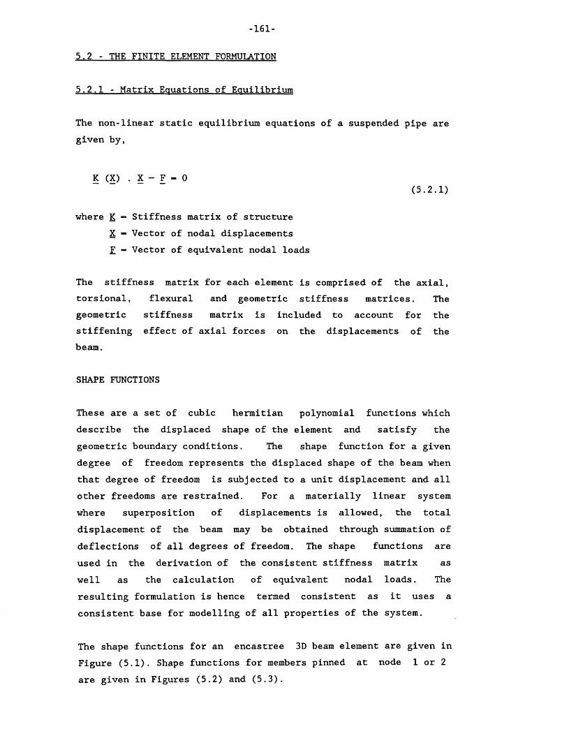
-161-

5.2 - THE FINITE ELEMENT FORMULATION

5.2.1 - Matrix Equations of Equilibrium

The non-linear static equilibrium equations of a suspended pipe are given by,

K (X) . X - F - 0(5.2.1)

where K - Stiffness matrix of structure X - Vector of nodal displacements F - Vector of equivalent nodal loads

The stiffness matrix for each element is comprised of the axial, torsional, flexural and geometric stiffness matrices. Thegeometric stiffness matrix is included to account for thestiffening effect of axial forces on the displacements of thebeam.

SHAPE FUNCTIONS

These are a set of cubic hermitian polynomial functions which describe the displaced shape of the element and satisfy the geometric boundary conditions. The shape function for a given degree of freedom represents the displaced shape of the beam when that degree of freedom is subjected to a unit displacement and all other freedoms are restrained. For a materially linear system where superposition of displacements is allowed, the totaldisplacement of the beam may be obtained through summation of deflections of all degrees of freedom. The shape functions are used in the derivation of the consistent stiffness matrix as well as the calculation of equivalent nodal loads. The resulting formulation is hence termed consistent as it uses a consistent base for modelling of all properties of the system.

The shape functions for an encastree 3D beam element are given inFigure (5.1). Shape functions for members pinned at node 1 or 2are given in Figures (5.2) and (5.3).

-162-

CONSISTENT STIFFNESS MATRIX

The element stiffness matrix is a combination of the axial, torsional, flexural and geometric stiffness matrices.

The terms of the axial stiffness matrix are derived by assuming a linear variation of axial strain along the element. The elements of 1^ are given by,

kbar(iiJ) - m , i,j-1 and 7(5.2.2)

where (') represents differentiation with respect to x. The terms of the torsional stiffness matrix are given by,

ktorsion<i’J) - GJ V>J(x).^:(x) dx , i, j-4 and 10 0 J (5.2.3)

The terms of the flexural stiffness matrix are given by,

kflexure(1,J) " EI V>7(x).^7(x) dx , i,j-2,3,5,6,8,9,11,12

(5.2.4)

The combined resulting member stiffness matrix for an encastree beam element is given in Figure (5.4). Figures (5.5) and(5.6) give the terms of the member stiffness matrices for beam elements pinned at node 1 or 2.

Structures subjected to large axial loads exhibit a different form of stiffness property referred to as geometric stiffness. This represents the contribution of the axial force towards resisting the flexural deformations of the element.

The elements of the geometric stiffness matrix are obtained by assuming a linear variation of the axial force of the form,

-163-

T(x) - T + 6T (^-)(5.2.5)

where: T — Axial force at node 1 (Tensile positive)ST — Change in axial force from node 1 to 2

These are given by,

*Ltt(x).*!(x) dx ,i,j-2,3,5,6,8,9,11,12

0 J(5.2.6)

The elements of the geometric stiffness matrix for an encastree beam element are given in Figure (5.7). Figures (5.8) and (5.9) give the same matrix for a member pinned at node 1 or 2.

Although Equation (5.2.6) is mathematically consistent with the Finite Element formulation presented, and has exclusively been used in the past, it lacks physical compatibility with the problem. This shortcoming may be illustrated by considering the governing equation of a beam including axial effects (see Clough and Penzien(1982)),

EI + T „ fdx« 1 d2x (5.2.7)

with the symbols having their usual meanings. Depending on the signand magnitude of T, the general solution of the differentialequation has three possible forms,

For T < 0 : y(x) — A sinaL + B cosaL + Cx + D /C oo\(D.Z.O)

For T > 0 : y(x) - A sinhaL + B coshaL + Cx + D ( 5 2 9 )

For T - 0 : y(x) = Ax3 + Bx2 + Cx + D 2 ^

where A, B, C and D are constants to be determined from the boundary conditions and a-|T/El|. Examination of the above equations shows that the cubic shape functions are only valid for

-164-

the case (T=0). If Equations (5.2.8) and (5.2.9) are alternatively used, the geometric stiffness matrix will be coupled to the flexural stiffness matrix. The terms of the combined matrix for an encastree circular beam section are shown in Figure (5.10).

The use of Equations (5.2.8) to (5.2.10) provides a more accurate accurate representation of the geometric stiffness effect. Although, the error may be small for lower values of a, for some flexible riser applications where T is typically large and El is small in comparison, the error can be significant.

EQUIVALENT NODAL LOADS

For a consistent representation of the intermediate loadings between the nodes these must be converted to a set of equivalent nodal loads which will produce the same effect on the structure as the original load distribution.

If the transverse load distribution is represented by a function f (x) for the range (0— ►L), then the equivalent nodal loads are given by,

The contribution of axial and torsional loads is similarly obtained through integration using their respective linear shape functions. If the magnitude of axial or torsional load along the element is assumed constant, the integration will be equivalent to placing half the total load on the member at each node of the element.

Figures (5.11),(5.12) and (5.13) present equivalent nodal loads for linear-uniform, linear-partial and point loads on an encastree beam element. Figure (5.14) and (5.15) give the equivalent nodal loads for a linear partial load on a beam pinned at node 1 or 2. Further loading conditions are given in Weaver(1980).

0f(x).V>i(x) dx ,i ,j=2,3,5,6,8,9,11,12

(5.2.11)

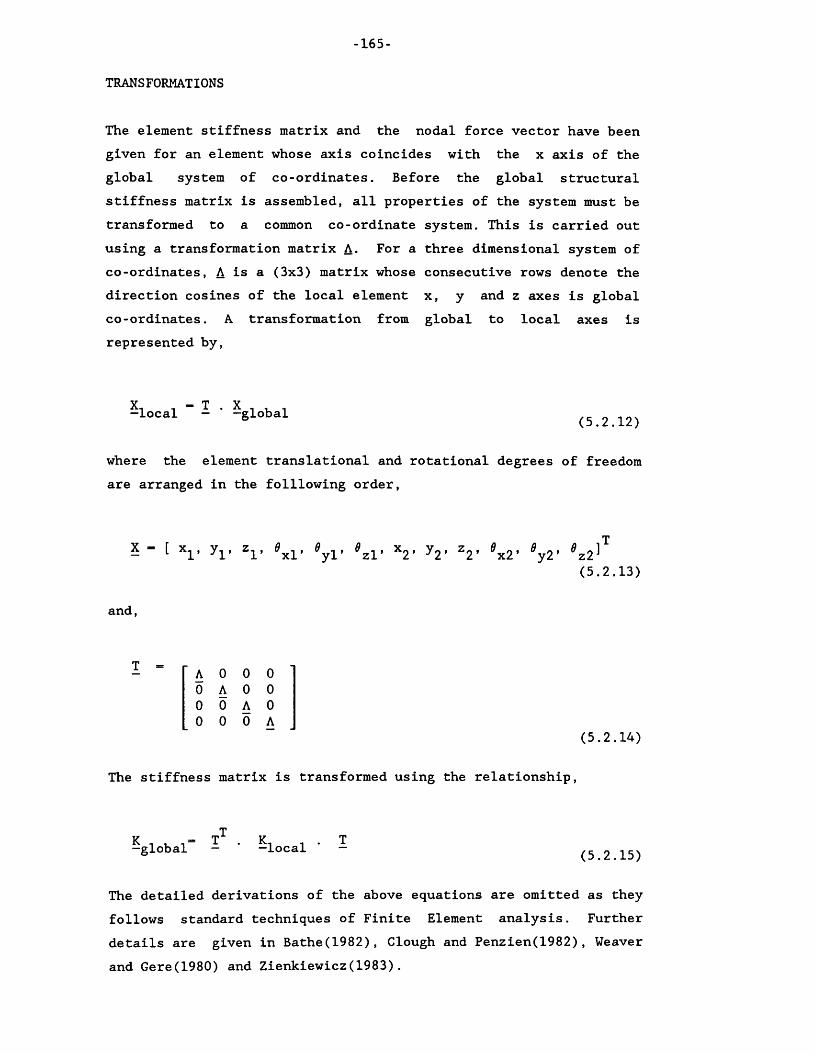
-165-

TRANSFORMATIONS

The element stiffness matrix and the nodal force vector have been given for an element whose axis coincides with the x axis of the global system of co-ordinates. Before the global structural stiffness matrix is assembled, all properties of the system must be transformed to a common co-ordinate system. This is carried out using a transformation matrix A. For a three dimensional system of co-ordinates, A is a (3x3) matrix whose consecutive rows denote the direction cosines of the local element x, y and z axes is global co-ordinates. A transformation from global to local axes is represented by,

Xn , = T . X . , .-local - -global

where the element translational and rotational degrees of freedom are arranged in the folllowing order,

X [ x1’ y r V xl’ yl’ zl’ *2’ y 2 ’ 2’ x2’ y2’ » 1 z2(5.2.13)

and,

A 0 0 00 A 0 00 0 A 00 0 0 A

(5.2.14)

The stiffness matrix is transformed using the relationship,

K . , T . K. - . T-global - -local - (5 2 15)

The detailed derivations of the above equations are omitted as they follows standard techniques of Finite Element analysis. Further details are given in Bathe(1982), Clough and Penzien(1982), Weaver and Gere(1980) and Zienkiewicz(1983).

-166-

5.2.2 - Boundary Conditions

For the purpose of static analysis, the ends of the pipe aremodelled by three translational and three rotational springs. The arrangement of these springs is illustrated in Figure (5.16). These springs provide control on the boundary conditions and help the examination of the effects of end fixities on the performance ofthe pipe. Either pipe end may also be modelled as a pinned joint.

5.2.3 - Prescribed Nodal Displacements

It is sometimes necessary to examine the effects of prescribeddisplacements along the pipe on its stress state. Examples include quasi-static analysis of a pipe subjected to vessel motions and pipeline laydown and pick-up.

In the absence of external forces the static equation of equilibrium (5.2.1) becomes,

K.X - 0(5.2.16)

For a prescribed displacement of a given degree of freedom, the displacements of the pipe are first seperated into prescribed and unknown values. This is schematically illustrated by,

X = X + X,a D (5.2.17)

where: X^ - Prescribed displacementX^ - Displacements resulting from X^

X^ represents a vector containing the prescribed displacement at the appropriate degree of freedom and whose other terms are zero.

Partitioning the stiffness matrix in the same way, we have,

-167-

K . X + K .. X. - 0aa a ab T) (5.2.18)

This effectively represents partitioning of the prescribed degree of freedom out of the stiffness matrix and displacement vector.

X - - K '1 . ( K , . X, )-ab (5.2.19)

Having determined vector X& , it may be combined with X^ to yield the total pipe displacement vector resulting from the prescribed displacement. Finally, the virtual force vector which would effect displacements X^ can be calculated using,

F - K . ( X + X. )_b " _a (5.2.20)

In practice, the partitioning of the stiffness matrix is not necessary. Alternatively, the vector —X^ is first constructed and pre-multiplied by K. Then, the rows and columns of the stiffness matrix corresponding to the prescribed degree of freedom are zeroedand unity is inserted in the diagonal position. The correspondingdegree of freedom in the force vector is then zeroed whichuncouples that degree from the equations. The solution of theresulting equations yields the vector X with a zero entry for thecLprescribed degree of freedom. This entry is then replaced by the value of the prescribed displacement.

-168-

5.3 - STATIC LOADS ON THE PIPE

The total static load on the riser is composed of the following:

a) Self-weightb) Internal and external pressure forcesc) Fluid dragd) Internal flow

The self-weight of the pipe produces lateral and axial components which may be integrated using methods outlined in Section (5.5).

Forces arising from internal and external fluid pressures may be calculated using a buoyancy analogy - see Sparks(1979), Sparks et al.(1982), Sparks(1984), Mc.Iver and Olson(1981) - or moreaccurately using an exact integration of fluid pressures over the inner and outer surface areas of the pipe - see Chakrabarti and Frampton(1982) or Young and Fowler(1978). A series of results for such integrations in two and three dimensions were presented in Chapter 3.

The fluid drag force is a measure of the resistance of the pipe to the flow of fluid in which it is immersed. The drag force on a cylindrical element placed with its axis perpendicular to the flow is given by,

F, - p C l L |U I U d ° (5.3.1)

For a flow at oblique incidence to the pipe, the velocity vector isresolved into components tangential and normal to the pipe axis.The normal component is treated as a transverse load and iscalculated using the above formula. The tangential component isoften neglected or integrated using the above formula but with acoefficient (C.) much smaller than for normal drag, d

Expressions for internal flow forces are given in Chapter 2. For a static case, a uniform flow is assumed and the calculated forces are distributed uniformly along the element.

-169-

5.4 - SOLUTION OF NON-LINEAR EQUATIONS OF EQUILIBRIUM

5.4.1 - Direct Iteration Method

The Direct Iteration Method is used to obtain the exact equilibrium solution of a non-linear system of equations. The method requires an approximate starting solution vector and its convergence characteristics are dependent on the nature of the problem considered but more heavily on the accuracy of the starting vector. For most problems involving suspended pipes, the catenary equations provide an accurate approximation to the pipe profile and hence the latter requirement is satisfied.

Consider a first solution of the equation of equilibrium (5.2.1),

(5.4.1)

where K0 represents the tangent stiffness matrix. Using the new set of displacements, X^, the stiffness matrix may be updated and used to obtain a further approximation,

X - K.'\,. F-n -(n-1) -n (5 4 2)

A measure of error is provided by,

E = X - X,n (n (5.4.3)

Two alternative convergence criteria may be used. Firstly the dot product E.E may be employed, which is equivalent to,

X _ X. < e X, -| v I-n -(n-1) I I -(n-1) | (5.4.4)

where e is a specified tolerance. Equation (5.4.4) presents a mathematical convergence criterion. Alternatively, a physical

-170-

criterion may be used involving the work done by the force F^. This is stated as,

F . [X - X, nJ < «| -n -n -(n-1) | (5 4 5)

The method is schematically illustrated in Figure (5.17) and a flow-chart provided in Figure (5.18).

5.4.2 - Improved Direct Iteration Method

The shortcoming of the basic Direct Iteration method is in its inability to allow for deformation dependence of loading. For some flexible riser applications where the equilibrium geometry undergoes substantial changes during loading, the resulting solution may be inaccurate in a physical sense despite being in mathematical equilibrium. It must be noted that the Direct method, nevertheless, includes the non-linearities of the stiffness matrix resulting from tensile force variations under load and that the deformation dependence of loads is a secondary source of non-linearity. The experience in this work suggests that the Direct method is a very efficient, easy to program and fast way of solution of non-linear static problems of types encountered with flexible riser applications. It would therefore be disadvantageous to resort to incremental techniques which are by definition less accurate except with a large number of steps and using equilibrium iterations. To overcome this difficulty, a modified version of the Direct method has been devised.

The new method, which is hereafter referred to as the Improved Direct Iteration Method, is a logical extension of the direct method where two nested iterations are performed. The inner iteration follows the basic Direct approach and the outer loop is used to ensure that the residual forces resulting from deformation dependent loading are equilibrated. Starting from a known equilibrium geometry, the full loading is applied and the displaced shape calculated using the basic method. The geometry is then updated and the full load vector for the new profile re-calculated. The residual force is defined as the difference between this vector

-171-

and that from the previous step and shows the amount of forcing that has been applied in shortfall or in excess. The residual force vector is then applied as an adjustment and the basic method is again employed to iterate for equilibrium. It is important to note the physical reasons behind the generation of the residual force vector. The calculated force at the end of a given iteration step is different to that at the start of the step by exactly the amount that has become transformed into tensile forces in the pipe. In order for the overall energy of the system at any step to remain constant, the residual force needs to be subtracted from the forcing at the following step. Experience with this procedure has shown that after the first step which typically takes between two to five basic direct iterations, subsequent steps use one or two inner iterations each. The total number of outer iterations for deformation dependence of forces rarely exceeds three steps. It must be noted that the above comments solely apply to flexible pipe applications discussed in this work and are not necessarily true of other systems.

As seen from the schematic illustration of the method in Figure(5.19), point A is first calculated using direct iterations. Thedifference between the original force vector and that at thedisplacement state Xj is then calculated and applied to the system which takes the system geometry to X2 and point B. Note that thestiffness matrix used at point A is different from the tangentstiffness matrix at the end of the first inner iteration loop represented by line OA and must be calculated for the updatedgeometry at Xj. If this re-calculation is omitted, the number of subsequent iterations will increase and more computational effortwill be required. It must be emphasised that the kernelconsideration in the use of the Improved Direct Iteration method is that at the end of each inner iteration for tensile forces, the structure is in equilibrium with the forces applied thereonto. In a physical sense, given that the loading is notably deformation dependent, this condition is not satisfied until the end of the analysis. However,in a mathematical sense, the structure remains on its equilibrium plane throughout the analysis and hence after all force adjustments have been applied, the resulting equilibrium solution will represent the true equilibrium state.

-172-

5.4.3 - Incremental Solution Technique (Deferred Averaging)

Incremental solutions involve loading the structure in a series of steps and re-calculating the stiffness matrix at each stage. The method may also be combined with intermediate equilibrium iterations to prevent excessive divergence from the exact solution. A large selection of incremental methods exist which are alternative combinations of intermediate and direct methods. In this section one such method is proposed which is named the Incremental Method with Deferred Averaging.

Using AX^ to represent the displacement vector resulting from the load vector AF at step n,

AX - K. ,. . AF -n -(n-1) -n (5 4 6)

which allows the calculation of stiffness matrix for step n. However, the exact stiffness matrix for step n may be expressed as,

K = [a K + j3 K, ,. ]_n ^-(n-l) (5 4 ? )

where a + f3 = 1. In the absence of information on the nature of the problem considered, ct=0.5 and y9=0.5 present one possible scheme. We then have,

K* - \ [ K + K. .,]n 2 n (n 1) (5.4.8)

The actual force which would cause the latest set of displacements may be expressed as,

AQ = K* . AX“n “n n (5.4.1)

However, only AF^ has been applied. The excess force applied may be calculated from,

-173-

F_ - F - AQ - i [ K - K . ,. ] . X-* -n -n 2 -n -(n-1) -n (J 4J(f)

F a should therefore be added back to the system at the next step ofloading. Equation (5.4.6) is therefore modified to the following form,

AX - K,"1,. . ( AF + F. )" (n_1) -* (5.4.11)

The method is schematically illustrated in Figure (5.21) and should be compared with Figure (5.22) which schematically shows the deferred averaging procedure. The proposed method provides a correction at each step and has two major advantages over the iterative techniques. Firstly, it is much faster and more efficient than the intermediate iteration techniques as it only involves one matrix multiplication and one matrix addition. The second advantage relates to the formulation of iterative techniques which usually use the stiffness matrix at the start of the step for residual force elimination at the end of the step. Consequently, if the system stiffness is changing rapidly through a step, or especially if its second derivative changes sign within a step, divergence of the solution may result. In contrast, the proposed method uses what is equivalent to an average stiffness for each step - hence the title deferred averaging. This technique will tend to force the solution to follow the equilibrium path. A flow-chart for incremental analysis with deferred averaging is given in Figure (5.23). To confirm the suitability of the method in preference to the conventional techniques, a simple non-linear single degree of freedom system whose stiffness was a cubic function of the displacements was used for a series of numerical tests. The following qualitative results were obtained:

- For large step sizes, the method gave a lower error than the basic incremental method for all cases considered.

- For relatively large step sizes, the results of the method were in error by about 5% whilst for the same step size, the conventional method was 35% in error.

-174-

- For a 20 step simulation which is typical for engineering analyses, the results of the new method were 0.5% in error whilst a 7% error was noted with the conventional method.

- For a target accuracy of 1%, the conventional method required 74 steps which on inclusion of intermediate iterations reduced to 17 steps and with the proposed method only required 7 steps.

Similar results were obtained for a quintic stiffness system which confirmed the suitability of the method qualitatively. Later finite element simulations provided further confirmation of these findings and showed the method to be capable of accommodating quite strong non-linearities. Further details and illustrative results are given in Chapter 8.

5.4.4 - Hybrid Methods

Hybrid methods are the result of a combination of the direct and incremental analysis procedures. The philosophy behind the use of these methods is that of avoiding the inaccuracies of incremental methods and evading the divergence problems associated with direct methods. A typical hybrid method is illustrated schematically in Figure (5.24) where at the end of each loading step, a series of direct iterations are performed to prevent a gradual divergence from the exact solution as seen in Figure (5.21). The presented version of the method is one of many alternatives which are available. The choice of the required combination of methods is often a function of the particulars of the given problem. Strictly speaking, the Improved Direct Iteration Method and the Incremental Method with Deferred Averaging which have been formulated in this work are also hybrid methods which have been purpose designed for the specific problem. The method illustrated in Figure (5.24) is a widely known technique and uses the stiffness matrix at the start of each step for carrying out the equilibrium iterations at the end of that step. This algorithm is commonly known as the Newton's Method. Sometimes a modified version of this method is utilised where the stiffness matrix is updated continuously during intermediate iterations. This would involve further computational effort and more decompositions of the stiffness matrix at each iteration. For some non-linear systems, this method may offer a

-175-

higher rate of convergence. The incremental method developed in this work includes an option for intermediate iterations using both forms of Newton's approach. A special version of the Hybrid method is required in the solution of flexible riser problems involving incremental shifting of one end of the pipe to its equilibrium position. These are discussed in the following section.

5.4.5 - Incremental Shifting Procedure

A specialised combination of the direct and incremental methods is used for analysis of flexible riser cases where due to initial indeterminacy of shape, it is not possible to obtain a direct solution from the catenary equations. Such situations result from a non-uniform buoyancy distributions or the existence of severalbuoyancy and clumped weight sections. In such cases, the only meansof obtaining the equilibrium profile is by starting from a known pipe geometry, usually a straight configuration and shifting one of the pipe extremities to its required final position. Whilst simple in outline, such procedures are of great complexity in implementation. The difficulties are caused by the ill-conditioned nature of the governing equations for these pipes. As mentioned earlier, these arise from the large differences in magnitudes of axial and flexural rigidities of the pipe. A survey of severalalternative methods has been presented in Chapter 2 and adiscussion of the relative merits of these methods has already been presented in the introduction to this Chapter. It was pointed out in the latter that the selected approach is due to Vogel and Natvig(1986). Although the fundamentals have been kept the same, the solution procedure has been developed on the basis of the direct and incremental methods discussed earlier and is different from that used by Vogel.

The large pipe displacements involved in shifting the pipe to its equilibrium geometry mean that in analysis,

a) The loading must be assumed deformation dependent.b) Rigid body rotations must be distinguished from curvature

induced rotations.c) The effect of second order rotations on pipe axial forces must be

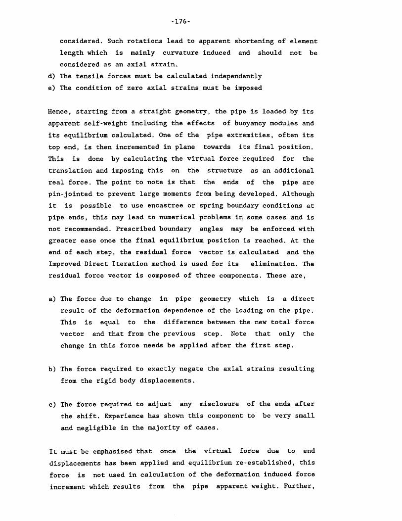
-176-

cons idered. Such rotations lead to apparent shortening of element length which is mainly curvature induced and should not be considered as an axial strain.

d) The tensile forces must be calculated independentlye) The condition of zero axial strains must be imposed

Hence, starting from a straight geometry, the pipe is loaded by its apparent self-weight including the effects of buoyancy modules and its equilibrium calculated. One of the pipe extremities, often its top end, is then incremented in plane towards its final position. This is done by calculating the virtual force required for the translation and imposing this on the structure as an additional real force. The point to note is that the ends of the pipe are pin-jointed to prevent large moments from being developed. Although it is possible to use encastree or spring boundary conditions at pipe ends, this may lead to numerical problems in some cases and is not recommended. Prescribed boundary angles may be enforced with greater ease once the final equilibrium position is reached. At the end of each step, the residual force vector is calculated and the Improved Direct Iteration method is used for its elimination. The residual force vector is composed of three components. These are,

a) The force due to change in pipe geometry which is a direct result of the deformation dependence of the loading on the pipe. This is equal to the difference between the new total force vector and that from the previous step. Note that only the change in this force needs be applied after the first step.

b) The force required to exactly negate the axial strains resulting from the rigid body displacements.

c) The force required to adjust any misclosure of the ends after the shift. Experience has shown this component to be very small and negligible in the majority of cases.

It must be emphasised that once the virtual force due to end displacements has been applied and equilibrium re-established, this force is not used in calculation of the deformation induced force increment which results from the pipe apparent weight. Further,

-177-

this should not be carried through to the next step as its effect ceases to continue after the equilibrium has been established. The strain balancing force vector is used as a means of imposing the zero strain condition. This force is simply computed by calculating the apparent axial strains in member co-ordinates, calculating the forcing required to neutralise these and maintain a constant member length. This is then transformed to global co-ordinates and combined with forcing from all members to form the system strain balancing force vector.

Having established the basics of the procedure, there remains two unresolved problems; namely, the calculation of tensile forces and bending moments along the pipe. Amidst all methods available, the simplest is undoubtedly that due to Vogel(1986) who has used a basic understanding of the behaviour of catenaries to advantage and proposed that the tensile force distribution may be computed by considering the catenary profile formed between the end of the buoyancy modules on the vessel side and the top connection at the vessel. The profile and characteristics adopted by this catenary are almost identical to those of a simple catenary suspended between these two points. Given the pipe length in this region and their equilibrium separation, the tensile force at the top of the pipe may be computed and the remaining tensile forces derived by forming the element force vectors and systematically subtracting the axial components from the calculated values of effective tension until the lower pipe end is reached. This approach was found elegantly simple and accurate for all present cases of practical interest.

The bending moments may be calculated after subtraction of the rigid body rotations from the member end rotations - see McNamara and 0'Brien(1986), O'Brien et al.(1987), or O'Brien and McNamara(1988). However, this would involve a series of computations and a moderate amount of computer work. Vogel and Natvig(1986) have demonstrated that the simplest means of calculating the bending moments is from the pipe curvatures through multiplication by the flexural rigidity. The pipe curvatures may themselves be derived by a variety of means. In this work these were calculated by fitting a circular arc to sets of three

-178-

consecutive nodes in space and taking the inverse of the radius of the fitted circle. This method was found to provide a very fast means of calculation of bending moments as the curvatures themselves needed to be calculated at each step for transformation of element matrices and element force vectors. The accuracy of the fitted curve may be increased easily by including more points and increasing the order of the fitted polynomial from two in the case of a circular arc to three and higher. Nevertheless, unless large element sizes and curvatures are present, such exercises are not considered necessary.

-179-

No (x) tf'(x) ^"(x)

1X

L

1

L0

2X

1 - 3 (-)2 + L

X2 (-)3

L-

X X 2 6 — + 6 —

L2 L3

6 12x

L2 L3

3X

1 - 3 (-)2 + L

X2 (-)3

L-

X X 2 6 — +6 —

L2 L3

6 12x

L2 L3

4X

L

1

L0

5X

- x ( 1 - - L)2 -1

4x 3x2

L L2

4 6x

L L2

6X

x ( 1 - - L)2 1

4x 3x2----- + ----

L L2

4 6x

L L2

7X

( 1 - - ) L

1

L0

8X

3 (-)2 - 2 L

X(")3L

X X 2 6 - - 6 -

L2 L3

6 12x

L2 L3

9X

3 (-)2 - 2 L

X(-)3L

X X 2 6 - - 6 -

L2 L3

6 12x

L2 L3

10X

( 1 - - ) L

1

L0

11X 2(— ) ( 1 - L

X- ) L

2x 3x2 2 6x

L L2 L L2

12X 2

- (— ) ( 1 - L

X- ) L

2x 3x2--- + ----

L L2

2 6x

L L2

Figure 5.1 — Shape Functions for an Encastree Element

-180-

No t/> (x ) (x) ^"(x)

X 11 - — 0

L L

3x x3 3 3x2 3x2 1 ----+ — ----+ ---- —

2L 2L3 2L 2L3 L3

O 3x x3 3 3x2 3x•3 X I "

2L 2L3 2L 2L3 L3

X 14 - — 0

L L

5 0 0 0

6 0 0 0

X 17 ( 1 - - ) ---- 0

L L

Q3x x3 3 3x2 3x

O2L 2L3 2L 2L3 L3

Q3x x3 3 3x2 3x

2L 2L3 2L 2L3 L3

X 110 ( 1 " " ) ---- 0

L L

1 1 X X 3 1 3x2 3x11

2 2L2 2 2L2 L2

X X 3 1 3x2 3x12 ----+ — ----+ ------ —

2 2L2 2 2L2 L2

Figure 5.2 — Shape Functions for an Element Pinned at Node (1)

-181-

No rj> (x) 1>' (x) V>”(x)

X 11 - - 0

L L

3x2 x3 3x 3x2 3 3x2 1 - --- + --- — — + --- — — + —

2L2 2L3 L2 2L3 L2 L3

3x2 x3 3x 3x2 3 3x3 1 + — — + --- --- + —

2L2 2L3 L2 2L3 L2 L3

X 14 — — 0

L L

C 3x2 x3 3x 3x2 3 3xD X + "

2L 2L2 |

L 2L2 L L2

3x2 x3 3x 3x2 3 3x6 x ----------+ -------- 1 ----------+ -------- — — —

2L 2L2 L 2L2 L L2

X 17 ( 1 ~ - ) ------ 0

L L

Q3x2 x3 3x 3x2 3 3x

O

2L2 2L3 L2 2L3 L2 L3

o3x2 x3 3x 3x2 3 3x

y2L2 2L3 eo

1 d

i1 i L2 L3

X 110 ( 1 - - ) ------ 0

L L

11 0 0 0

12 0 0 0

Figure 5.3 — Shape Functions for an Element Pinned at Node (2)

-182-

EA -EAK ( 1, 1 ) ---- K ( 1, 7 ) ------

L L12EI 6EI

2, 2 ) ------ - K ( 2, 6 ) ------ -L3 L2

-12EI 6EI2, 8) ------- K ( 2,12)------ -

K

K

K

K

K

K

K

K

K

K

K

K

L3 L212EI —6EI

3, 3 ) ------Z K ( 3, 5 ) ------- 2L3 L2

-12EI —6El3, 9 ) -------2 K ( 3,11)------- 2

L3 L2GJ -GJ

4, 4 ) ---- K ( 4,10)------L L4EI 6EI

5, 5 ) ^ K ( 5, 9 ) ------^L L22EI 4EI

5,11) * K ( 6, 6) -------L L

-6EI 2EI6, 8 ) ------- K ( 6,12)------ -

L2 LEA 12EI

7 , 7 ) ---- K ( 8, 8) ------- ^L L3-6EI 12EI

8,12)------ K ( 9, 9 ) ------ 2L2 L3

6EI GJ9,11)----- ^ K (10,10)-----

L2 L4EI 4EI

11,11)----- ^ K (12,12)-------

Note : Only the non-zero upper diagonal terms are shown Matrix is symmetrical about upper diagonal

Figure 5.4 — Stiffness Matrix for an Encastree Element

-183-

EA -EAK ( 1, 1 ) ---- K ( 1, 7 ) -----

L LEl —3EIzK ( 2, 2) = 3 — K ( 2, 8) ------ -L3 L3

3EI 3EIK ( 2,12)---- K ( 3, 3 ) -----2

L2 L3—3EI —3EI

K ( 3, 9 ) ------^ K ( 3 f 11) ------ 1L3 L2

GJ -GJK ( 4, 4 ) --- K ( 4,10)-----

L LEA 3EI

K ( 7, 7 ) --- K ( 8, 8) ----- 5-L L3—3EI 3EI

K ( 8,12)------ K ( 9, 9 ) -----2L2 L3

3 El GJK ( 9,11) ^ K (10,10)-----

L2 L3EI 3EI

K (11,11) X K (12,12)------ -


Figure 5.5 — Stiffness Matrix for an Element Pinned at Node (1)

-184-

EA -EAK ( 1, 1 ) ---- K ( 1, 7 ) ------

L L3EI 3EI

K ( 2, 2) - ---- K ( 2, 6) ------ -L3 L2

—3EI 3EIK ( 2, 8) ------ K ( 3, 3 ) ------ 1

L3 L3—3EI —3EI

K ( 3, 5 ) ------ 2 K ( 3, 9 ) ------- *L2 L3

GJ -GJK ( 4, 4 ) ---- K ( 4,10)------

L L3EI 3EI

K ( 5, 5 ) Z K ( 5, 9 ) ----------1L L2

3EI —3EIK ( 6 , 6) --------- K ( 6 , 8) ------------- -

L L2EA 3EI

K ( 7, 7 ) ---- K ( 8, 8) ------ -L L33 El GJ

K ( 9, 9 ) -----£ K (10,10)----L3 L


Figure 5.6 — Stiffness Matrix for an Element Pinned at Node (2)

185-

K ( 2, 2)6T + 36T

5L

K ( 2, 8) - - K ( 2, 2)

K ( 3, 3) - K ( 2, 2)

K ( 2, 6)T + 6T

10K ( 2,12) ----

10K ( 3, 5) - - K ( 2, 6)

K ( 3, 9) - K < 2, 8)

(4T+6T)L K ( 5, 5) ----------

K ( 5,11) - -

30(2T+5T)L

30

K ( 6, 8) = K ( 3, 5)

K ( 3,11) - - K ( 2,12)

K ( 5, 9) - - K < 3, 5)

K ( 6, 6) - K ( 5, 5)

K ( 6,12) - K ( 5,11)

K ( 8, 8) - K ( 2, 2) K ( 8,12) - K ( 3,11)

K ( 9, 9) - K ( 3, 3)

(4T+35T)L K (11,11) - ---------

30

K ( 9,11) - - K ( 8,12)

K (12,12) - K (11,11)


Figure 5.7 — Geometric Stiffness Matrix for an Encastree Element

-186-

6T 36TK ( 2, 2 ) -----+ K ( 2, 8) - - K ( 2, 2)

5L 8L T

K ( 2,12) - - K ( 3, 3) - K ( 2, 2)5

K ( 3, 9) - K ( 2, 8) K ( 3,11) --- K ( 2,12)

K ( 8, 8) - K ( 2, 2) K ( 8,12) --- K ( 2,12)

K ( 9, 9) « K ( 8, 8) K ( 9,11) --- K ( 8,12)

T £TK (11,11) - ( - + — )L K (12,12) - K (11,11)

5 8

Note : Only the non-zero upper diagonal terms are shown Matrix is symmetrical about upper diagonal Element is assumed axially symmetric

Figure 5.8 — Geometric Stiffness Matrix for an Element Pinned at Node (1)

6T 336T T + 6TK ( 2, 2 ) -----+ K ( 2, 6) --------

5L 40L 5

K ( 2, 8 ) - - K ( 2, 2) K ( 3, 3) - K ( 2, 2)

K ( 3, 5) - - K ( 2, 6) K ( 3, 9) - K ( 2, 8)

L 35TK ( 5, 5) - - ( T + --- ) K ( 5, 9) - - K ( 3, 5)

5 8

K ( 6, 6) - K ( 5, 5) K ( 6, 8) - - K ( 5, 9)

K ( 8, 8) - K ( 2, 2) K ( 9, 9) - K ( 3, 3)

Note : Only the non-zero upper diagonal terms are shown Matrix is symmetrical about upper diagonal Element is assumed axially symmetric

Figure 5.9 — Geometric Stiffness Matrix for an Element Pinned at Node (2)

-187-

K

K

K

K

K

K

K

K

K

K

K

K

K

1, 1)

2 , 2 )

2 , 8)

3, 3)

3, 9)

4, 4)

5, 5)

5.11)

6, 8)

7, 7)

8.12)

9,11)

11,11)

EA

L2k3

L2-2k,

L22k3

L2—2k,

L2GJ

L

k.

2-k,

LEA

L-k.

K

K

K

K

K

K

K

K

K

K

K

K

1, 7)

2 , 6 )

2,12)

3, 5)

3.11)

4,10)

5, 9)

6 , 6)

6.12)

8 , 8)

9, 9)

10,10)

12,12)

-EA

L

LSL~k3L

~k3L

-GJ

L

kl

k2

2k,

L22k,

L2GJ

L

k.

For a member in tension:

El aL[— (l+/?)aL coshaL + sinhaL]ki - -

L — (l+/?)aL sinhaL + 2(coshaL—1)

El aL[(l+/3)aL — sinhaL]k ^ -

L — (l+/3)aL sinhaL + 2(coshaL—1) k3 - ki + k2

Figure 5.10 - Improved Geometric Stiffness matrix for an Encastree Element (continued on next page)

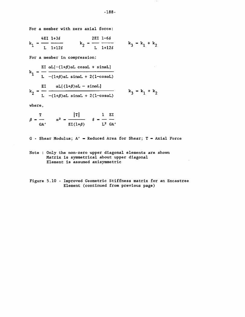
-188-

For a member with zero axial force:

4EI 1+35 2EI 1-65k - ------------------ k _ ------------------ k« = k1 + k_

L 1+125 L 1+125

For a member in compression:

El aL[— (l+/?)aL cosaL + sinaL]1 L — (l+;8)aL sinaL + 2(1—cosaL)

El aL[(l+/?)aL — sinaL]k? ----------------------------------------k_ - k- + k«

L -(l+^)aL sinaL + 2(l-cosaL)

where,

T |T| 1 El- — a2 - 5 — — —

GA' EICl+^S) L2 GA'

G - Shear Modulus; A' - Reduced Area for Shear; T - Axial Force

Note : Only the non-zero upper diagonal elements are shown Matrix is symmetrical about upper diagonal Element is assumed axisymmetric

Figure 5.10 - Improved Geometric Stiffness matrix for an Encastree Element (continued from previous page)

-189-

F< 1) - 0

F( 2) — ( 7W1 + 3W2 )L/20

F( 3) - ( 7VX + 3V2 )L/20

F( 4) - 0

F( 5) - - ( 1.5V1 + V2 )L2/30

F( 6) - ( 1.51^ + W2 )L2/30

F( 7) - 0

F( 8) - ( 3WX + 7W2 )L/20

F( 9) - ( 3VX + 7V2 )L/20

F(10) - 0

F(ll) - ( V l + 1.5V2 )L2/30

F(12) --- ( Wx + 1.5W2 )L2/30

^1’ ^2 Load intensity per unit length in direction of localelement Y axis at nodes (1) and (2)

V^, V2 - Load intensity per unit length in direction of localelement Z axis at nodes (1) and (2)

Figure 5.11 - Equivalent Nodal Loads for a Uniform Trapezoidal load on an Eneastree Element

-190-

F( 1) - 00 a a 3 0 2 0

F( 2) - a(b-a)+ -(b2-a2)----(b3-a3)+(---------- )(b4-a4)+ — (b5-a5)2 L2 2L3 4L2 5L3r e e 3c 2r

F( 3) - e(b-a)+ — (b2—a2)----(b3-a3)+(---------- )(b4-a4)+ — (b6-a5)2 L2 2L3 4L2 5L3

F( 4) - 0

F( 5) — [^(b2-a2) - ( ^ - £-) (b3—a3)+(-^— - £-)(b4-a4)+ -— (b6-a5)]2 3L 3 4L2 2L 5L2

a 2 a 0 a 0 0F( 6) - — (b2—a2)— (------ ) (b3—a3)+(-------- )(b4-a4)+ ----(b5-a6)

2 3L 3 4L2 2L 5L2

F( 7) - 0

a 3 0 a 2 0F( 8) ----(b3-a3)+(--------- ) (b4—a4)----- (b5-a6)

L2 4L2 2L3 5L3e 3c e 2r

F( 9 ) ----(b3—a3) + (--------- ) (b4—a4)----- (b5-as)L2 4L2 2L3 5L3

F(10) - 0

e r e rF(ll) [(---------) (b4—a4)---- (b3—a3)+ --- (b5-a5) ]

4L2 4L 3L 5L2a 0 a 0

F(12) - (-------- ) (b4—a4)--- (b3—a3) + --- (b6-a6)4L2 4L 3L 5L2

W,-W= ( — — - ) a - W - 0 . a

b — a aV-v

f = ( ) ( - V - r.ab — a a

= Load intensity per unit length in direction of localelement Y axis at distances a and b from node (1)

V , — Load intensity per unit length in direction of localelement Z axis at distances a and b from node (1)

The start and end points of loading are assumed to be at a and bfor loading in both the Y and Z directions

Figure 5.12 - Equivalent Nodal Loads for a partial Trapezoidal Loadon an Eneastree Element

-191-

F( 1) - 0Si Si

F( 2) - P [ 1 - 3(—)2 + 2(-)3 ] 7 L L

b bF( 3) - P [ 1 - 3(-)2 + 2(—)3 ]

Z L L

F( 4) = 0

bF( 5) - -P b ( 1 - - )2

La

F< 6) - P a ( 1 - - )2 7 L

F( 7) - 0

a aF( 8) - P [ 3(-)2 - 2(—)3 ]

7 L Lb b

F< 9) - P [ 3(—)2 - 2(—)3 ]Z L L

F(10) - 0

b2 bF(ll) - P^ (— ) ( 1 “ “ )

Z L La2 a

F(12) - -P (— ) ( 1 - - )7 L L

Note : P — Point Load magnitude in local element Ypy «= Point load magnitude in local element Za = Distance of P from node (1) of element Vb — Distance of P-7 from node (1) of elementz

directiondirection

Figure 5.13 Equivalent Nodal Loads for a Point Load on an Eneastree Element

-192-

F< 1) - 0

3a a 0 — 0 0F( 2) - a(b-a)--- (b2-a2)H (b4-a4 )+-(b2-a2 ) + — (b3-a3)H--- (b5-a5)

4L 8L3 2 2L 10L3H £ f -f r

F( 3) - (b-a)--- (b2—a2)H----(b4-a4 )+-(b2-a2)+ — (b3-a3H --- (b5-a5)4L 8L3 2 2L 10L3

F( 4) - 0

F( 5) - 0

F( 6) - 0

F( 7) - 0

3a a 0 0F( 8) ----(b2—a2)-----(b4—a4)+ — (b3-a3)------ (b6-as)

4L 8L3 2L 10L3H £ r f

F( 9 ) ----(b2—a2)-----(b4—a4)+ — (b3-a3)------ (b5-a6)4L 8L3 2L 10L3

F(10) - 0

£ £ r rF(ll) - — (b2—a2)-----(b4—a4)+ -(b3-a3)-------(b5-a5)

4 8L2 6 10L2a a 0 0

F(12)----- (b2—a2 )+ ---(b4—a4)— -(b3-a3)+ ---- (b5-as)4 8L2 6 10L2

W -WP - ( - 2 — ^ ) o - W - p.a

b - a aV.-V

r - ( !* ) f - V - f-ab - a 3

- Load intensity per unit length in direction of local element Y axis at distances a and b from node (1)

V&> — Load intensity per unit length in direction of localelement Z axis at distances a and b from node (1)

The start and end points of loading are assumed to be at (a) and(b) for loading in both the Y and Z directions

Figure 5.14 - Equivalent Nodal Loads for a Partial TrapezoidalLoad on an Element Pinned at Node (1)

-193-

F< 1) - 0

—a « P 33 PF( 2) *= a(b—a)H--(b3— a3)-l— (b4—a4)+— (b2—a2 )— — (b4—a4) + (b5 a5)

2L2 8L3 2 8L2 10L3* r 3C r

F( 3) - £(b—a)H--(b3—a3)-I— (b4—a4)+— (b2—a2)— — (b4-a4) + ---(b5—a5)2L2 8L3 2 8L2 10L3

F( 4) *= 0

-£ c -£ r 3r -rF( 5) - — (b2—a2)h— (b3—a3)H— (b4-a4)- -(b3-a3)H— (b4-a4)H--- (b5-a5)

2 2L 8L2 3 8L 10L2a — a a /3 3(3 /3

F( 6) ---(b2—a2)n— (b3-a3)n— (b4-a4)+-(b3-a3)---- (b4-a4)H--- (b5-a5)2 2L 8L2 3 8L 10L2

F( 7) - 0

a a 3/3 fiF( 8) ----- (b3—a3)-----(b4—a4)+ ---(b4-a4) ------- (b6-a5)

2L2 8L3 8L2 10L3

F( 9 ) ----- (b3—a3)-----(b4—a4) + ---(b4-a4) ------- (b5-a5)2L2 8L3 8L2 10L3

F(10) - 0

F(ll) - 0

F(12) - 0

w,-wp = ( — — - ) a - W - p . a

b — a aV.-V

r - (--- ) ( - v - r.ab — a a

W& , = Load intensity per unit length in direction of localelement Y axis at distances a and b from node (1)

V , — Load intensity per unit length in direction of localelement Z axis at distances a and b from node (1)

The start and end points of loading are assumed to be at a and b for loading in both the Y and Z directions

Figure 5.15 - Equivalent Nodal Loads for a Partial Trapezoidal Loadon an Element Pinned at Node (2)

- 194-

Static Bounday Conditions

KzKez

o

Kx, Ky, Kz - Translational Spring Stiffnesses

Kex, Key, Kez - Rotational Spring Stifnesses

Figure 5.16 - Static Boundary Conditions

- 195 -

Direct Iteration Method Schematic

Force

X 2 X 3 Xi

F - Total Force Vector Kj - Tangent Stiffness Matrix at Iteration (i) X o- Starting Nodal Geometry Array X i- Displacement Array at Iteration (i)

figure 5.17 - Direct Iteration Method Schematic

- 196 -

YES

Calculate forces and moments

Update geometry Xo= Xo +_X(i)

Calculate nodal displacements X(i) = K(M)

Calculate new tensile forces TO) and update by the initial catenary values

Re-calculate tangent stiffness matrix K(i) using T(i)

Calculate initial catenary equilibrium profile under effective self-weight and calculate tensile forces

Direct Iteration Method for Static Analysis

Check for convergence:

I [ K(i) ■ K(i-l) ] . X(i) I < Tolerance

Assemble tangent stiffness matrix_Ko and nodal geometry array Xo using catenary values and

calculate the total force vector X f° r profile

Figure 5.18 - Flow-chart for Static Analysis with Direct Iteration Method

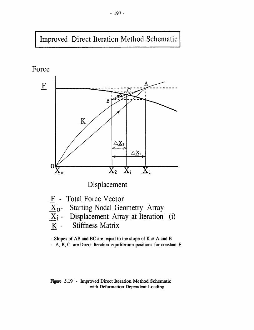
- 197 -

Improved Direct Iteration Method Schematic

Force

AXA X

0Xo

Displacement

F - Total Force VectorX 0- Starting Nodal Geometry ArrayXi - Displacement Array at Iteration (i)K - Stiffness Matrix

- Slopes of AB and BC are equal to the slope of K at A and B- A, B, C are Direct Iteration equilibrium positions for constant F

Figure 5.19 - Improved Direct Iteration Method Schematic with Deformation Dependent Loading

- 198 -

NO

YES

Stop

Check for convergence of residual force

Copy initial force vector to residual force vector

Calculate total force vector for new geometry & compute the residual force vector F ■

Calculate the initial starting profile Xq tangent stiffness K_0 tensile forcesT0and total force vector _F0

Improved Direct Iteration Method for Static Analysis

Update nodal geometry array to the new equilibrium position X j = X_j_i + A X. . and update tensile forces

Form the tangent stiffness matrix K_j for current geometry and calculate the displacements and tensile forces using the Direct iteration method with current residual forces

Figure 520 - Flow-chart for Static Analysis with Improved Direct Iteration Method

- 199-

Incremental Method Schematic

Force

F

exact

Displacement

F - Total Force Vector Kj - Tangent Stiffness Matrix at Step (i) X o- Starting Nodal Geometry Array

_Xi- Displacement Array at Step (i)A_F - Force Increment

_Xexacr Exact Displacement Vector Solution

Figure 5.21- Incremental Method Schematic

- 20 0 -

Incremental Method Schematic with Deferred Averaging

Force

AF - Jres

-res

A F

F - Total Force Vector K - Stiffness Matrix

J£o- Starting Nodal Geometry Array _X i - Displacement Array at Step (i) a _F - Force IncrementF res- Residual Force

Figure 5.22- Incremental Method Schematic with Deferred Averaging

NO

YES

Output Results

Last Increment ( i=N) ?

Assemble tangent stiffness matrix using current geometry and tensile forces

Read total number of increments ( N ) and zero X(i)

Calculate force increment for step (i)_F =A_F + 0.5 x [K(i-l)- _K(i)] .X_(i-1)

Calculate initial catenary equilibrium profile under effective self-weight and calculate tensile forces

Incremental Method for Static Analysis

Calculate Displacement Increment Calculate element forces and moment and add to existing

Update nodal geometry array byX(i)

Assemble tangent stiffness matrix K(i) and nodal geometry array using catenary values and

calculate the total force vector _F(i) for this profile Calculate the force increment a F= F / N

Figure 5.23 - Flow-chart for Static Analysis with Incremental Method Using Deferred Averaging

- 2 0 2 -

Hybrid Method Schematic

Force

F

_£±o

Displacement

F - Total Force Vector Kj - Tangent Stiffness Matrix at Step (i)

_Xo- Starting Nodal Geometry Array _Xi- Displacement Array at Step (i)A_F - Force Increment

-Xexact- Exact Displacement Vector Solution

Figure 5.24 - Hybrid Method Schematic

-203-

CHAPTER 6 : FINITE ELEMENT DYNAMIC ANALYSIS

6.1 - INTRODUCTION

Dynamic analysis of suspended pipes requires an extension of the finite element formulation outlined in Chapter 5 to include fluid inertia, added-mass and drag effects. This chapter is devoted to the development of the required components of the dynamic analysis technique used in this work. Initially, the element mass and added mass matrices are developed. Alternative representations of the structural damping matrix are discussed using the conventional representation of structural damping where this is assumed to be of Rayleigh type. This type of damping assumes that the structural damping matrix is a proportional combination of the structural mass and stiffness matrices. The advantage of this assumption is that the structural damping matrix may then be diagonalised in the same way as the mass and stiffness matrices. One of the methods discussed allows different damping coefficients to be prescribed to each mode of vibration and thus provides better control on representation of a damped system where, for instance, certain modes require to be damped heavily. However, this method provides zero damping for all remaining modes of vibration. For time domain analyses, unless a modal approach is used, usually, all modes of vibration require some degree of damping to avoid uncontrolled accumulation of spurious oscillation in these modes. For such cases, the traditional form of Rayleigh damping is considered where the structural damping matrix is simply composed of a proportional summation of the stiffness and structural mass matrices.

The formulation of a frequency domain method is then described. This is based on the modal analysis and is used for analysis of response to regular wave excitations. The use of a frequency domain approach implies linearity; at least temporally. For this reason, the non-linear drag force needs to be linearised. A study of the available linearisation techniques showed several suitable alternatives to be available. The selected method is due to Krolikowski and Gay(1980) and provides good accuracy combined with great ease of implementation. Figure (6.1) illustrates a series of results which have been quoted from the above paper. These show

-204-

comparative results for several cases of current and wave combination. The Figure has been provided as an illustration of the accuracy to be expected from the method for different ratios of current velocity to realtive velocity as well as serving as a rough guide on interpretation of the results to be presented later in this work. Linearisation of the drag force separates this force into its fluid and structural velocity dependent terms. This results in a drag-damping term which multiplies the structural velocities and can, therefore, be transferred to the left hand side of the equations of motion and combined with the structural damping term. Techniques used in linearisation of the drag force differ widely. The resulting drag damping matrices are, therefore, closely related to the linearisation method. This problem is treated differently in time domain analyses where the drag force is calculated in its full non-linear form on the right hand side of the equations of motion instead of being treated as a combined load and damping effect.

Despite their speed and versatility, the validity of frequency domain techniques is limited to exciation frequencies away fromstructural resonant frequencies. Moreover, their extension to analysis of irregular sea states involves restrictive assumptions which, coupled with the necessity for linearisation of the non-linear drag term, reduce their accuracy below acceptable thresholds. In such cases, time integration of the governingequations must be carried out. Time domain methods are invariably more expensive in run time and storage requirements but are capable of modelling the non-linear drag exactly as well as being capable of analysis of structural response to multi-frequency excitations. Several methods of time integration are available, a collection of which is given in Bathe(1982). The most widely used and purportedly one of the most accurate is the Newmark-j0 method which is based on difference expressions for structural parameters between successive time steps. The development of this method for flexible riser analysis is provided in this Chapter. Additionally, to enable anexamination of the effects of structural and loadingnon-linearities on the riser response, an intermediate equilibrium iteration scheme has been derived. The algorithm uses an approach very similar to the deferred averaging procedure described in the

-205-

context of incremental analysis in Chapter 5.

The dynamic influences of internal flows of variable density are studied next. Methods are proposed in this chapter for modelling internal flow induced excitation of flexible risers in the frequency and the time domains. The equations in the time domain are shown to be more accurate and capable of modelling these forces in conjunction with wave and vessel induced loads. Since investigation of such coupled loadings on flexible risers has not been attempted in the past, the proposed model is of interest in removing a major area of uncertainty from the analysis. Experimental investigation of internal flow induced oscillations are reported in Chapter 7 whilst the implications of simultaneous internal flow, wave loading and vessel induced excitation are studied in Chapter 8.

Dynamic analysis of flexible risers requires the inclusion of the pipe end dynamic displacements and rotations. These form a series of dynamic boundary conditions and are illustrated schematically in Figure (6.2). The most convenient method of incorporating these boundary conditions is to calculate the virtual force system resulting from these displacements. These forces can be imposed on the system as real forces which will effect the required displacements and rotations at ends. The development of this method in both the frequency and the time domains is described in detail.

This chapter also discusses the methods used in description of the sea state which are common to all dynamic analyses. Simulation of sea states involves computation of the fluid properties such as instantaneous wave height, particle velocities, particle accelerations and dynamic pressure changes. The motion of a single water wave is described by a wave theory, several of which have been postulated in the past. Each theory has limits on its applicability which are usually defined in terms of non-dimensional ratios of water depth, wave-length, wave steepness and wave height. The most commonly used wave theories are described by Sarpkaya and Isaacson(1981) which includes details on their mathematical development. The scope of this work excludes an examination of the choice of wave theory on the structural response. The Linear (Airy)

-206-

wave theory, being by far the most widely used in engineering, was hence chosen. The formulation of the Linear wave theory is based on a sinusoidal representation of the wave surface profile. Attenuation of water particle velocities and accelerations are represented by hyperbolic functions decaying with depth whilst their space and time variations are assumed to be harmonic. The choice of the Linear wave theory is particularly suitable for frequency domain analysis where its simple periodic nature is utilised in the solution of the resulting equations. Time domain techniques, however, do not rely on such features and accommodate different wave theories with greater ease.

Simulation of irregular seas has traditionally been carried out through a decomposition of the wave height spectrum into a series of frequency bands. A wave height is then associated with each band in proportion to the square of the spectral height at the central frequency of that band. The irregular sea is then assumed to be a combination of all such waves whose phases are chosen at random from a uniform distribution. An alternative approach, first suggested by Tucker and Challenor(1984), has additionally been implemented. The use and characteristics of these methods are addressed and the approach used for simulation of an irregular sea-state for time domain analysis is detailed.

-201-

6.2 - DYNAMIC EQUATIONS OF EQUILIBRIUM

The dynamic equations of motion may be derived using a variational formulation which involves minimisation of thetotal potential energy of the system. The derivation may be found in Clough and Penzien(1982), Bathe(1982) and Zienkiewicz(1983). The dynamic equations of motion in matrix form are given by,

M X + B X + K X - F(6.2.1)

CONSISTENT MASS MATRIX

The physical mass matrix of the member in axial and flexural degrees of freedom can be evaluated using the shape functions discussed earlier. The individual terms are given by,

m (i»j) - p A s J s s ^i(x).^j (x) dx , i,j-2,3,5,6,8,9,11,12( 6 . 2 .2 )

The physical mass matrix for the torsional degrees of freedom is given by,

^i(x).^j(x) dx i,j-4 and 7(6.2.3)

The combined physical mass matrix is given in Figure (6.3). The contribution of the mass of internal pipe fluid may be included by modifying (6.2.2) although the axial and torsional components of the inner pipe fluid must be excluded from the resulting matrices.

CONSISTENT ADDED MASS MATRIX

To preserve the consistency of the formulation, the added mass matrix is modelled using the same shape functions. This effectively assumes that the added mass of the element can berepresented by the mass of a cylinder of fluid occupying the

-208-

same position in space as the physical mass where the volume of this hypothetical cylinder is dictated by the coefficient of added mass. Eliminating the contribution of the axial and torsional mass, this gives,

The full added mass matrix is given in Figure (6.4).

HYDRODYNAMIC LOADING

The hydrodynamic force per unit length on the pipe element is given by the modified Morison equation which can be written as,

The first two terms represent the inertia force and the third deals with the effect of hydrodynamic drag on the element. Ifthe added mass term is taken to the left hand side of the equations of motion and combined with the physical mass term, the remaining expression becomes,

m (i,j) - p A (C - 1) a o o m V>i(x).^j (x) dx , i, j-2, 3 ,5,6 , 8 ,9,11,12

(6.2.5)

( 6 . 2 . 6 )

-209-

6.3 - DESCRIPTION OF THE SEA STATE

For the puropse of this work, the Linear (Airy) wave theory was selected. Although certain environmental conditions may require the use of other wave theories, such studies are beyond the intended scope of this work and will therefore not be pursued further. The Linear wave surface profile is illustrated in Figure (6.5) and is expressed by the equation,

2 sin(kx—cot)(6.3.1)

The horizontal and vertical fluid velocities are given by,

u

v —

<oH cosh[k(y+d)] ,2 sinh(kd) U j

e ^ sin(kx-cot)

f n a ye ^ cos(kx-cot)

Shallow Water

Deep Water

Shallow Water

Deep Water

(6.3.2)

(6.3.3)

and the corresponding accelerations, by differentiation,

— c°sh[k(y+d)_] Cos(kx-wt) Shallow Water2 sinh(kd)

— e ^ cos(kx—cot) Deep Water(6.3.4)

— sin(kx-cot) Shallow Water2 sinh(kd)

— —^ e ^ sin(kx-cot) Deep Water(6.3.5)

The shallow water wave length is determined iteratively from,

-210-

L — ^ — tanh(—=— ) =- < 0.7 (approx.)2* L L _ (6.3.6)

whilst the deep water wave length is given analytically by,

^ > 0 . 7 (approx.)(6.3.7)

For the purpose of a frequency domain analysis, the complex form of the fluid velocity and acceleration terms are used whereas time domain simulations use the forms given above directly. In regular wave analysis, the sea state is simulated using a single wavewhilst for irregular wave analysis, the conventional simulation is based on a superposition of a series of regular waves of different heights travelling with relative phases which are randomly chosen in the interval (0— *2n) from a unifrom distribution. The height and period of each wave is chosen from the wave height spectrum, anexample of which is given in Figure (6.6). The conventionalprocedure for simulation of an irregular sea state may besummarised in the following steps:

gT22tt

1- Divide the wave spectrum ^nn(w) into a series of frequency bands. This is usually carried out using regular frequency intervals of Aw with the central frequency in each band and its associated spectral amplitude represented by w^ and ^nn(w£)•

2- Calculate the wave height for the central frequency of each band from the relationship,

rf. - J 2 S (w.) Aw 1 nn 1 (6.3.8)

3- Generate a set of (i) phases in the range (0— 2 ) from a uniform distribution.

4- Generate the combined wave properties using a summation over all wave components using expressions of the form,

-211-

N»?(x,t) - 2 »7isin(kix - a^t + ^ )

1-1 (6.3.9)

Tucker and Challenor(1984) have shown that not only the phases but also the wave heights, are random variables. Twoalternative, but equivalent, methods have been postulated for accurate simulation of irregular seas. The first uses the expression,

Nn(x,t) = S c . sin(k.x - w.t + <f>.). - l l i l

(6.3.10)

where c^ are random variables chosen from a Rayleigh distribution of rms - 7[2Snn(toi)Awi] . Alternatively, the wave is generated using the expression,

Nij(x,t) — S [ a^ sin(k^x — w^t) + b^ cos(k^x — w^t) ]

where a^ and b^ are independent random variables chosen from aGaussian distribution with common variance a 2 - [S (w.)Aw.l.nn l iJTucker has shown that these techniques are identical.

The most commonly used spectra are the JONSWAP (Joint North Sea Wave Project) and the Pierson-Moskowitz spectra. The JONSWAP spectrum is given in Hasselmann(1973), and, Brebbia andWalker(1979) which define it by the equation,

(w - w )2 mS (w) - -f- exp[— t (—4)] 7 2o 2u>2nn w6 4 w4 mm

Hs v 2a ~ w — wm ~ """ NgTz:ct — 0.07 ,for w " a - 47r3 (7^ 72)

0.09 ,for w > w b m(6.3.12)

where tt>m is the frequency at which the wave energy is a maximum and 7 is typically taken as 3.30. An alternative empirical description

-212-

of the JONSWAP spectrum for typical North Sea conditions has been derived by Isherwood(1987) which allows its expression in terms of the significant wave height, Hg and the mean wave period, T . These results are based on a best fit approximation to large quantities of data collected over several years.

The Pierson-Moskowitz spectrum (see Pierson and Moskowitz(1964)) may be described analytically by the equation,

S (w) - ^§- exp[— ^ (^4)] nn w6 4 o)4m (6.3.13)

where a is the same as for the JONSWAP spectrum. The spectrum in terms of the sig is expressed as,terms of the significant wave height, Hg and the mean wave period

/ \ Hl/3 Tz r o > T z 5 r 1 /wTzx—4 ,nn “ 8 ^ — 1 2ff 1 eXp[ " ? ] « , ,/x(6.3.14)

-213-

6.4 - REGULAR WAVE ANALYSIS IN THE FREQUENCY DOMAIN

MODAL ANALYSIS

The frequency domain analysis is carried out using a modal analysis technique. The dynamic equations of motion are,

M X + B X + K X - F(6.4.1)

where (.) represents differentiation with respect to time. The matrix of mode shapes, $, obtained from solution of the free undamped equations of motion is used to transform the above equation to generalised coordinates P, defined by,

X = 3> P(6.4.2)

Twhich upon substitution and premultiplication by $ yields,

* * * * *M P + B P + K P - F(6.4.3)

where,

onM - * M « , B - ® B ® , K - * K ® , F - $ F

(6.4.4)

The mass and stiffness matrices are now diagonalised but the damping matrix, in general, remains non-diagonal. The structural damping matrix may be assumed proportional to themass and stiffness matrices so that the orthogonality conditions apply (Rayleigh Damping). However, the drag-damping matrix in general can not be diagonalised using the modal orthogonality relations. In other applications, the non-diagonal terms can beignored to allow the equations to remain uncoupled. In either case, equations reduce to a set of N independent linear equations with the generalised response in mode i being given by,

where w is the circular frequency of excitation and subscript (ii) refers to the diagonal terms (all quantities being scalar). The total response is then obtained by summing the modal responses for all degrees of freedom. In practice, the contribution of the higher modes of vibration to the total response is small and only the first few modes are needed to determine the total response to sufficient accuracy. A slightly larger number of modes is normally used for the calculation of dynamic forces. It must be noted that this formulation is based on the assumption that the structural response is at the same frequency as the excitation frequency.

STRUCTURAL DAMPING MATRIX

The structural damping matrix is derived assuming a Rayleigh type damping which assumes both stiffness and mass proportionality. It can be shown that as a result of modal orthogonality conditions - see Clough and Penzien(1982) and Warburton(1982)- the resulting structural damping matrix, when normalised with respect to the mode shapes, is diagonal. The diagonal terms of the normalised structural damping matrix are given by,

Bs. . = 2 £. <j>. Ms..11 i i 11 (6.4.6)

where M s ^ refers to the diagonal term of the normalised structural mass matrix, is the natural frequency in mode i and is the damping coefficient in mode i. All non-diagonal terms are zero. The structural damping matrix may be obtained by reversing the normalisation outlined earlier,

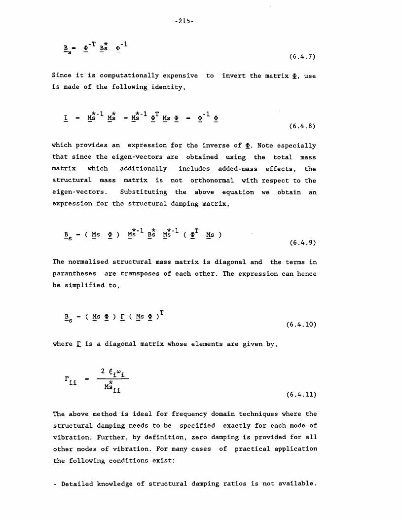
-215-

-T * -1B - $ Bs $S (6.4.7)

Since it is computationally expensive to invert the matrix use is made of the following identity,

*-1 * *-1 T -1I - Ms Ms - Ms * Ms * - f t(6.4.8)

which provides an expression for the inverse of $. Note especially that since the eigen-vectors are obtained using the total mass matrix which additionally includes added-mass effects, the structural mass matrix is not orthonormal with respect to the eigen-vectors. Substituting the above equation we obtain an expression for the structural damping matrix,

B - ( Ms £ ) Ms'1 Bs Ms'1 ( £T Ms )S (6.4.9)

The normalised structural mass matrix is diagonal and the terms in parantheses are transposes of each other. The expression can hence be simplified to,

B = ( Ms $ ) £ ( Ms $ )T S (6.4.10)

where £ is a diagonal matrix whose elements are given by,

2 ? 1 “iii *Ms..(6.4.11)

The above method is ideal for frequency domain techniques where the structural damping needs to be specified exactly for each mode of vibration. Further, by definition, zero damping is provided for all other modes of vibration. For many cases of practical application the following conditions exist:

- Detailed knowledge of structural damping ratios is not available.

-216-

- Structural response is restricted to the first few modes only.- The structure is designed such that its natural frequencies are well away from expected loading frequencies to avoid resonance. This implies that the effect of structural damping on the response is likely to be small.

In such cases, it is possible to use a common alternative to the above formulation which reduces the calculation effort significantly. The method is based on the assumption that the structural damping matrix may be represented by a combination of the structural mass and stiffness matrices. This may be written as,

B - a M + 0 KS (6.4.12)

Constants a and fi may be calculated to provide exact damping ratios in two modes of vibration say Wj and w2 . With this method, all other modes also receive some degree of damping which may be calculated if necessary. Figure (6.7) illustrates that modes falling outside the range between these two frequencies are quite heavily damped with the largest and smallest frequencies receiving the greatest degree of damping. This feature of the method is particularly useful in the time domain analyses where heavy damping of the lower and higher modes of vibration is often essential for numerical stability reasons. If the normalised version of Equation(6.4.2) is equated to Equation (6.4.6), we have,

2 u w — a + flw2T T T (6.4.13)

Re-writing this for the two modes of consideration and solving the resulting system of two simultaneous equations gives,

2(/iiW2— /i2W l)a — - w2

Ct), Ct)„ ^(6.4.14)

and

-217-

(6.4.15)

which, provided the required damping ratios in the two modes of interest and the corresponding eigen-values are known, enables the calculation of the structural damping matrix. The damping characteristics of the resulting matrix are illustrated in Figure (6.7) which also shows the variation of the damping ratios for modes other than specified.

LINEARISATION OF DRAG FORCE

The non-linear square law behaviour of the drag force requires that this force be replaced by an equivalent linear expression for a frequency domain analysis. This procedure is carried out by following the approach described by Krolikowski and Gay(1980). This involves expanding the non-linear drag force into a Fourier series and neglecting the higher harmonics. Gelb and Vander Velde(1968) have shown that for systems where the input to the non-linearity is sinusoidal, the mean-squared approximation error is minimised by using such a Fourier expansion of the non-linear output. The linearised drag force in the presence of a steady current is represented by,

+ C u c —cn (6.4.16)

where,

C - p C.R 2 uT.T ' A n A iw o d o c for u > u c — m

3u2u

c i usin (— ) um m m m

for u < u c m(6.4.17)

and

-218-

p C ,R o d ou

r ^ u2 + u2 2 m c

— [ [l+2(7T U

for u > u c — m

u , u 3u I u— )2]sin (— ) + — ) 1 - (— ) u u u um m m m

for u < u c m

with u — I u — x I m 1 —n —n 1 (6.4,18)

which in the absence of current reduces to,

C - -r— p C ,R u — xw 3ir o d o —n —n

C - 0 c(6.4.19)

(6.4.20)

Equation (6.4.16) can now be separated into two terms,

(6.4.21)

where,

f = C u + C u —e w —n c —cn

b x - C x — — w —n

(6.4.22)

(6.4.23)

Equation (6.3.5) can now be written in the form,

f - f. + f — b x1 6 n (6.4.24)

The quantities f^, f^ and b are derived using the virtual work principle. For a single element in local co-ordinates, the linearised drag force per unit length is given by,

-219-

f (x) - C (x) ( u(x) - y(x) ) + C (x) u (x)° (6.4.25)

where y(x) is used to define a structural velocity function. For a given set of nodal displacements, a^, the deflection profile of the element is given by:

y (x) - i> a , i-2,3,5,6,8,9,11,12(6.4.26)

where t}> represents the shape functions discussed earlier. Similarly the structural velocities are obtained from,

y (x) - rj> a , i-2 , 3 , 5 ,6,8 ,9 ,11,12(6.4.27)

Consider a virtual displacement 5W. The resulting virtual work is,

f.(x) 6W dx —a(6.4.28)

6w can in general be represented by,

6W = 8 a.l l (6.4.29)

Substitution gives,

V Cw (x)u(x)^idx - [S C (x)^.^.dxl a. + C (x)u (x)^.dx . c c /ri

(6.4.30)

Comparison with the general Lagrangian equations shows that the terms inside the brackets represent the generalised force for the i-th. degree of freedom. This gives,

Assume a linear variation of all quantities in each of the orthogonal planes xy and xz, of the form,

C (x) - ( 1 - £ ) C -+ < 7 ) C 0 w ' L wl L w2

Cc(x) - ( 1 - 5 ) ccl+ ( I ) Cc2

U (X) - ( 1 - 5 ) u x + ( 5 ) u 2

uc(x) - < 1 - I > ucl+ ( I > Uc2

U (x) - ( 1 - jr ) U x + ( jr ) U 2

(6.4.33)

(6.4.34)

(6.4.35)

(6.4.36)

(6.4.37)

where subscripts 1 and 2 refer to values at nodes 1 and 2. The terms of the equivalent linearised drag force are found by integrating Equation (6.4.31) and are given in Figure (6.8) where

and C£ represent the equivalent drag coefficients at nodes 1 and 2. The integration also yields the drag damping matrix whose terms are given in Figure (6.9).

Using the same approach it can be shown that the inertia force vector is given by,

f.— 1 7r R2 p C u(x) ij>. dx 0 0 m 1 2,3,4,6,8,9,11,12(6.4.38)

The terms of this vector are given in Figure (6.10).

-221-

DYNAMIC BOUNDARY CONDITIONS

The most convenient method of incorporating the boundary conditions resulting from the prescribed vessel motions is to calculate the virtual forces resulting from these displacements. These forces can then be imposed on the system as real forces which will produce the required displacements and rotations at the upper end of the riser. This procedure can be implemented by dividing the pipe motions into those due to pipe dynamics and those induced by the end motions. If we denote the end displacements by P^Pe displacements dueto end motions by X^, and pipe displacements due to wave kinematics by X, we have,

X_ _ . - X + X total e (6.4.39)

Considering vessel induced motions and in the absence of wave induced components, the pipe end displacements are substructured out using a static condensation approach where the prescribed degrees of freedom are moved to the last rows and columns of the system stiffness, mass and damping matrices. The pipe displacements vector due to vessel motions can be separated into the unknown displacements vector X _ and the prescribed displacements vector X^. This substructuring is obtained by simple subtraction where the last degrees of freedom of Xg relating to end motions alone are transferred to the null vector X and the remaining vector namedsX . The last rows of X corresponding to X are then zeroed. The t t §rows of X corresponding to unknown displacements are similarly 6zero. The equations of motion may now be written as,

M (X + X ) + B (X. + X ) + K (X + X ) = 0- -g' - v-t -g' - -t -g (6.4.40)

Since X , and its derivatives are known, we can take their related”gterms to the right hand side of the equations giving,

Sub-structuring of the degrees of freedom relating to known and unknown displacements is implicit in the equation. We can calculate the quasi-static displacements due to end motion by ignoring the dynamic terms on the left hand side. A more accurate method, however, would be to consider a,

( — u>2 M + iu B + K) X . ( M X + B X + K X )- - -t _ _ g _ _ g _ _ g (6.4.42)

type formulation and solve for the complex displacements due to end motions. It is, however, computationally advantageous to avoid forming the complex dynamic stiffness matrix given in parantheses on the left hand side of the above equation and it will be shown later that these terms may otherwise be accounted for without any loss of accuracy. We can write to a good approximation,

K X ( M X + B X + K X )-tt-s -tg-g -tg-g -tg-g (6.4.43)

where Xg denotes the quasi-static displacements and excludes the prescribed degrees of freedom, K refers to the top submatrix of K whose degrees of freedom correspond to the unknown displacements. The substructuring used is as follows,

’ K K X - ' X X - ■ 0-tt ~tg -tK K —S 0 “g X

. "gt ~gg . — . -g .

The mass and damping matrices are substructured in the same way asthe stiffness matrix. Note that the use of submatrices is asimplification permitted after substructuring and is a result ofthe null subvectors in X and X . X can now be calculated using,s g s

-223-

X K'J; [ X + B^ X + K X ]-s -tt -tg -g -tg -g -tg -gJ

X K"]; [ -w2 M + iu B + K 1 . X-s -tt -tg -tg -tgJ -g

X « r . X~s - -g

where,

r K"]; [ -w2 M + iw B. + K. ]-tt -tg -tg -tgJ

(6.4.44)

(6.4.45)

(6.4.46)

(6.4.47)

r, is the matrix of quasi-static mode shapes resulting from unit end displacements and Xg are displacements along the pipe resulting from the displacements of the end of the pipe. The complete pipe displacements due to end motions are given by,

X , - X + X-s+g -s -g (6.4.48)

Since the mass and damping effects were ignored in calculation ofXg , te above displacements will not be identical to X^. It is shownnext that this inaccuracy may be removed. Note that in matrixterms, X and X do not have shared degrees of freedom, i.e. X s g srepresents pipe motions due to X . Substituting £g+g f°r *-n Equation (6.4.41) gives,

M X + B X + K X [ ( M X + M. X + B X + B X + K X + K X ] tt s -tg-g -tt-s -tg-g -tt-s -tg-gJ(6.4.49)

This equation is easily seen to be out of balance by the error discussed. Equation (6.4.49) simplifies to,

M X + B X + K X - — [ <—tt— +^tg)V (5ttS +W (“tt£ +-tg)-81(6.4.50)

but from Equations (6.4.44) to (6.4.46) we have,

Substituting this into (6.4.50), reduces it to,

M X + B X + K X ( M X + B X )_ _ _ _ _ _ _tg_g _tg_g (6.4.52)

The right hand side represents the required out of balance force in Equation (6.4.50). Therefore, the dynamic component of support displacement may be represented as an effective force vector where,

F __ - — ( M r X + B r X )-eff - t t - - g - t t - - g (6 4 53)

This force accounts for the omitted terms in Equation (6.4.43) and should be combined with the dynamic force vector. In physicalterms, Equation (6.4.53) takes account of the dynamic effect of vessel motions. It should be pointed out that the above formulation was followed with a second objective in mind which was theuncoupling of the quasi-static and dynamic displacements. As illustrated above, this is possible, provided that the coupling force term (Equation (6.4.53)) is added to the dynamic forcingcomponent. This approach is later shown to offer significant simplifications to implementation of vessel induced motions in the time domain.

-225-

6.5 - REGULAR SLUG FLOW ANALYSIS IN THE FREQUENCY DOMAIN

The discussion in Chapter 3 dealt with a fluid of constant density. Slugs are, however, variant in their compositions and densities. The following derivation considers the effect of the flow of a slug with a variable density on the pipe. It must be noted that the following derivation considers the simultaneous effect of a steady and a time varying component since due to the conditions of continuity these may not be separated.

For a first approximation, consider a slug whose density is allowed to vary harmonically and is represented by,

p ( s) - p + p sin(ks + <f>) e1Wt i P (6.5.1)

where: p Q - Amplitude of density variationsP

k - Slug wave number - 2 n / slug wave length w - Slug circular frequency - 2tt / period <f> - Phase angle

If the total curved length to ends 1 and 2 of the element are denoted by sx and s2 , then the total change in mass across the element in Figure (6.7) is given by,

. iwt dM - P a k ^ e sin (ks + <f>) ds(6.5.2)

i p0A.e*Wt: [ cos (ks.+ <f>) - cos (ks„- <f>) ] k P 1 1 2 (6.5.3)

^ p^A^e^Wt [(cos ks^— cos ks^) cos <f> —

(sin ks^— sin ks^) sin <t> ](6.5.4)

Now, using stQp to represent the total curved length to top of the pipe, the dynamic pressure change at end 1 of the element can be found from the total change in the mass of slug above end 1 of the element.

-226-

dPx - P p g eiwt t0^ sin (ks + <f>) ds

£ P p g eiwt [ cos (ks^+ <f>) - cos (kstQp+ ]

(6.5.5)

(6.5.6)

Similarly,

dP2 - £ p^g eiwt [ cos (ks2+ <f>) - cos (kstQp+ ^) ](6.5.7)

The velocities and U2 are obtained using the equation for the total mass flow rate, Q,

Q -

u -A i [ P ±+ Pgsin (ks + <f>) eiwt]

(6.5.8)

(6.5.9)

giving,

U = U [ 1 + ^ si° L Ptin (ks + <f>) eiwt

-1

(6.5.10)

The change in velocity can be computed from

dU = U — Uo A. l p + p sin (ks+^) e i Piwt

(6.5.11)

hence,

dU - U— p_ sin (ks+^) e £ ________p ±+ P p S in (ks+^) e

iwt

iwt(6.5.12)

Now, using the same approach as in the static case and using the

-227-

same notations we have,

^2Ai^2 cos 2 _ ^lAi^l cos^i= P^^cosfl^— P2^icos^2+ (6.5.13)2 i2 sn 2 — lAil s-n i “ P si i- P2 is n 2_ + (6.5.14)

where: ?x - P1(statlc) + dPxP2 " P2(static) + dP2M - M . + dMstatic

Therefore, the forces exerted on the pipe are now given by,

fx - Ai[ ( p1 Up cos^^ ( P2+ P2Up cos^l

f - A t[ ( P-J + P - ^ \ ) sin0 + ( P2+ P2UP sin^2 ~ K &

(6.5.15)

(6.5.16)

Expressions for squares of velocities may be obtained from the Taylor expansion of equation (6.5.10)

-228-

6.6 - TIME DOMAIN ANALYSIS

The fundamental assumptions of a frequency domain analysis are that the loading is harmonic and the structural response to this loading is similarly harmonic and at the same frequency. The method is often used for analysis of multi-frequency input systems by assuming linear independence of outputs at different frequencies which permits superposition of responses at different frequencies. The forcing on pipes suspended in water is conventionally evaluated using Morison's equation. The non-linearity of the drag term in this equation invalidates superposition of responses.

Exact representation of non-linearities is, however, possible using time integration procedures. The development of numerical models in the time domain is often hindered by the realisation of their excessive computer time and storage requirements. With increasing resource and speed of present day computers, typical run times have been reduced to more realistic values. The accuracy provided by the time domain methods in modelling system non-linearities and their extreme ease of implementation now warrants their use as standard design tools. These methods are basically integration procedures in time and are based on finite-difference equations in time. Examples of these methods are provided by Bathe(1982) which includes a comparison of the relative merits of each method, as well as notes on their implementation. For the purpose of this work, the Newmark-/? method was chosen. This was based on the information provided by Bathe(1982) which indicates that the Newmark-/? method has zero period elongation and lowest amplitude decay rate amongst all other methods. The method is founded on combined finite-difference and Taylor's expansions for structural displacements, velocities and accelerations. These are expressed as,

—( t + A t ) ~ ? tXt + [(!-«) Xt + « (t+At) (6.6.1)

and,

" xt- + X. At + [(0.5 - a) X_ + a X. A<_J -(t+At) -t -t -t — (t+At) ^ 6

where a and 6 are constants chosen for numerical stability and accuracy, a and 6 are restricted to lie within the following bands,

6 >= 0.5 ; a >— 0.25 (0.5+6)2 ,, .( b . b .3)

The combination (5-0.5 , a-0.25) is the most popular and is referred to as the constant-average-acceleration method which results in an unconditionally stable scheme. Consider the dynamic equations of equilibrium at time (t+At),

- -(t+At) + - -(t+At) + - -(t+At) " -(t+At) (o.6.4)

Equations (6.6.1) and (6.6.2) may be solved to yield expressionsfor accelerations at time (t+At) in terms of the displacements attimes (t) and (t+At). First, to simplify the representation ofequations involved, the following notations are introduced,

o x x , o n» a i “ ~ A*- » a 2 “ ^ A*. > a 3 ” ■*" » a 4 " “ « 1“° a At2 ’ ai a At ’ °2 a At

a5- ^ — 2 ) ; a6- At ( 1 - 5 ) ; a,- t At(6.6.5)

The structural velocities at time (t+At) are then represented by,

X . . . - + a8 X_ + a7 X , _ _ s(t+At) t t (t+At) g g^

and structural accelerations as,

-(t+At) = a°( -(t+At) -t^ &2 -t 33 -t (6.6.7)

These expressions are substituted into Equation (6.6.4) and terms relating to time (t) are moved to the right hand side of the equation and combined with the force vector to give,

-eff(t+At)“ — (t+At)+ - (a°-t+ a2 -t+ a3 + - (a!-t+ a4-t+ a3-t)(6.6.8)

which is called the effective force vector. The equations of motion may now be expressed as,

-eff -(t+At) ” —eff(t+At) (6 6 9)

with,

K - K + a0 M + at B(6.6.10)

which is the effective stiffness matrix. Solution of Equations(6.6.9) yields the displacements of the structure at time (t+At).

DYNAMIC BOUNDARY CONDITIONS

Motions of the support vessel generate a dynamic boundary condition at the end of the riser which must be accommodated in the time integration algorithm. Theoretically, the same approach as in the frequency domain analysis may be used. However, the extended computational effort involved with such calculations meant that a compromise between accuracy and computational effort had to be found.

An updated Lagrangian method where at each time step the geometry of the structure is updated and equilibrium iterations are performed was rejected for two reasons. Firstly, such an approach requires equilibrium iterations at each step of integration involving repeated assemblage and factorisation of the stiffness matrix, an extremely time consuming approach. Secondly, for each updated geometry, not only vessel motions had to be calculated relative to the geometry, but more wastefully, the quasi-static mode shapes for the vessel motions at the next time step had to be re-evaluated. Although theoretically simple, the computational

-231-

effort involved in this apporach makes its practical useimpossible. A total Lagrangian approach based on the mean equilibrium geometry was the alternative choice. This method assumes that motions occur about a mean equilibrium geometry which is a condition satisfied for all cases to be considered in this work. As a result, the quasi-static vessel motion mode-shapes need only be evaluated once with respect to the equilibrium geometry and scaled up for the given vessel motions at each time step. Vessel induced accelerations and velocities may similarly be derived from these mode shapes by suitable scaling discussed later.

The difficulty remaining with this method was that of carrying out equilibrium iterations. The complication arises from the fact that once the vessel has been purturbed from the static equilibrium geometry, it oscillates about this and for a general case never returns to the exact same location. This can be visualised by considering an elliptical vessel motion envelope in surge and heave, for example. The centre of the ellipse corresponds the static equilibrium whilst its circumference represents the riser top motion trajectory. To calculate equilibrium iterations, the geometry needs to be updated, after which point, the remaining motions must be calculated with respect to the new equilibrated geometry. Although possible, this is a crude approach and willintroduce inaccuracies which will increase in proportion to distance from the new equilibrium geometry. A technique wasdeveloped based on separation of dynamic pipe displacements into wave and vessel induced components. The latter are accurately known in a quasi-static sense. Provided that fixed pipe dynamic displacements may be calculated to include the effective forcing due to vessel motions exactly, the total response may be obtained by summation of these components without inconsistency. It should be noted that the calculation of non-linear drag force must include the combined total displacements.

Given the transfer functions of vessel motion and their phases relative to the wave, for a wave spectrum composed of (n)frequencies, the riser top displacements, velocities andaccelerations in a given degree of freedom (j) may be described by the following equations,

-232-

^ HX - 2 X j sin(a> t+<f> ) , j-1,6J (6.6.11)

where X represents the transfer function normalised against the wave amplitude and ft is the transfer function phase at circular frequency The velocity and accelaration are calculated throughdifferentiation of these equations.

n UXI “ w x 9 cos(w t+^ .) , j-1,6J (6.6.12). . n „X - 2 - a>2 X £ sin(o> t+^ ) , j-1,6J (6.6.13)

Computation of these quantities is required at each time step. Using the quasi-static mode shape vector, r, the complete vessel induced displacement, velocity and accelaration vectors are givenby,

X. - X. r. X - X r . X - X r.J J J J J j J J j (6.6.14)

However, coupling with dynamic pipe displacements must be provided through the effective force vector which, as pointed out earlier, removes the imbalance from the equations. The effective forcing vector is given by,

nf -- - — .2- ( M X. + B X.) -eff l-l - -j - -J (6.6.15)

This approach was found to be the most economical and stable. The economy is achieved through the use of quasi-static mode shapes which are calculated once only for a given geometry. The instabilities relating to numerical problems associated with imposing the full vessel inertia term on the pipe were avoided using the proposed method. Inertia effects multiply structural accelerations which are second derivatives of displacements. As a result, small inaccuracies in displacements can give rise to much

-233-

larger errors in accelerations. Full vessel forcing has the effect of an impulse at each time step. This is a direct consequence of the discrete nature of the loading which is implicit in the analysis. Instabilities arise from error build up through summation of the effects of all such impulses and the lack of damping to enable adequate control of these errors without violating physical constraints on damping. These instabilities are difficult to avoid except by adopting a different formulation as carried out in this work or deriving the accelerations by direct means using an inversion of the mass matrix. The proposed method allows an exact match of prescribed and integrated end motions, simplifies the calculations considerably and avoids all instability problems.

-234-

6.7 - NON-LINEAR ANALYSIS IN THE TIME DOMAIN

Non-linearities encountered in the analysis of flexible riser systems may be grouped into structural, loading and material related categories. Non-linearities focused on in this work include those arising from changes in structural geometry during loading and the non-linear nature of the drag force. Equations of motion in the time domain are derived on the basis of a total Lagrangian formulation where all displacements are measured from the mean static position but provide the response continuity through equations relating parameters at a given time step to those at the previous step(s). For structures undergoing large translations in space, the use of a total Lagrangian formulation is clearly not possible. An alternative updated Lagrangian formulation is used in such cases where after a give number of time steps, the structural geometry is updated to equilibrium through a series of iterations. For typical flexible risers where the structural response is harmonic about a mean static configuration, the use of an Updated Lagrangian formulation is unnecessary and extremely expensive.

Neglecting large rigid body translations, local structuralnon-linearities such as the variable seabed boundary condition with the lazy-S and lazy-wave risers may be accommodated with accuracy through techniques based on intermediate equilibrium iterations. These iterations aim to remove instantaneous imbalances from the equations of motion. The imbalance is represented by,

A— (t+At) " - — (t+At)+ - — (t+At)+ - -(t+At) “ -(t+At) (6 ?

The forcing on the pipe is a function of the instantaneousdisplacements, velocities and accelerations of the pipe. Inaddition, the stiffness, mass and damping matrices of the pipe are modified by changes in its geometry. To accommodate such effects exactly, intermediate non-linear iterations are required. These involve calculation of a corrective displacement vector (AX) and its associated velocity and acceleration terms to eliminate te residual force vector. The direct iteration method used in the static analysis may be extended to the dynamic analysis by

-235-

incorporating the mass and damping effects. The equations for non-linear iteration take the form,

M y ( k ) . R v W + / K + K ' W w y ( k ) - f - F < k " 1 > (t+At) (t+At) — -(t+At) -(t+At) — (t+At) — (t+At)(6.7.2)

where

• (k)-(t+At)” l°cal PiPe tangent stiffness matrix after deformations

and(k—1)-(t+At)” loadinS calculated on geometry at iteration (k-1)(k)AX is given by the following expression, y (k) (o) a y (k)5(t+At>- *(t+At)+ “ (6 ? 3)

The trapezoidal rule may be used for time integrations. This corresponds to the Newmark-/3 method with a-0.25 and 5-0.5. the choice of these parameters is of lesser importance to non-linear analysis than to the time integrations. These parameters provide a system which is very closely related to the deferred averaging procedure used in conjunction with the incremental method. The expressions for velocities and accelerations thus become,

W W V (6.7.4)

*(t+At)“ *t + f < = W ) + *t> (O./.D)

Using the above three equations, expressions for velocity and acceleration at step (k) may be obtained.

y *. h / y(°^ + AX^k — X — X-(t+At) At — (t+At) — —t —t ^ -j

y = ^ / y ( ®^ 4. A y y \ _ ___—_ y _ y-(t+At) At2 ( -(t+At) - -t ' At -t -t y

Substitution in Equation (6.7.2) and rearranging gives,

-236-

[ t~2- M + f- B + K ] AX(k) - F - K >(k)AX(k)At* — A t — — — — — —

- s [ s * < > - h h ~ h i

- ® t St ( 5 ( ^ t ) “ 5t > - it 1 - I*'1' (6.7.8)

It is noted that the mass and damping terms on the right hand side of this equation are constant through the equilibrium iterations and only the force and geometry dependent terms are variant. Iteration for the force term is unnecessary, except for very large displacements. The stiffness dependent term, however, represents an equivalent forcing required to enforce the seabed displacement boundary condition. It is possible to use the extended deferred averaging procedure to carry out these iterations. The method which was described in Chapter 5, was found particularly efficient for this type of problem. In summary, the stiffness matrix is calculated for the displaced pipe state at step (k) and multiplied by the vector of displacement estimate to provide a new virtual forcing function. The pipe-seabed interface is modelled using a series of vertical springs uniformly distributed along the length of each finite element in contact with the seabed. The equivalent nodal spring stiffnesses in translation and rotation in the vertical plane are derived using the equivalent nodal load calculation procedure. During the equilibrium iterations, these spring stiffnesses are updated according to the last estimate of the displacements vector. The iteration convergence is checked using,

A X ^ - AX^k_1M < €1 (6.7.9)

where € represents a specified displacement tolerance. The velocityand acceleration correction vectors are finally computed fromEquations (6.7.6) and (6.7.7) and used to update the calculatedpipe parameters at time (t+At).

-237-

6.8 - REGULAR SLUG FLOW ANALYSIS IN THE TIME DOMAIN

Derivations presented in Section (6.5) involve approximations in calculation of fluid velocity variations, necessary for a frequency domain simulation. Furthermore, the use of frequency domain techniques has the following disadvantages:

- Due to the non-linear drag forcing and drag induced damping, combinations of wave loading and internal flow cannot be studied within the same frequency domain analysis. This excludes the exceptional cases where the slug frequency is equal to the wave frequency.

- The fluid velocity changes must be approximated by a Taylor series expansion of the steady and temporal components of the flow.

Non-periodic or discontinuous-periodic (rectangular) density changes may not be accommodated. A Fourier series type simulation of these flows may similarly not be attempted for reasons stated above.

These considerations leave time domain techniques as the only means of obtaining accurate results and discarding the above restrictions. The development presented here relies on the assumptions that:

- The fluids are Newtonian- The rate of mass flux is constant- The flow is of constant average velocity- The velocity of the gas relative to the fluid is zero- Friction head losses are negligible- The pressure and velocity changes occur at constant temperature

In simulation of internal flow along pipes of considerable length, such as those typically arising in offshore multi-phase fluid transportation, some of the above assumptions are clearly not permissible. For example, significant heat losses exist, large friction head losses occur, the fluid composition may change with temperature and flow Reynold's number and flow frequency or

-238-

regularity may alter as a result of changing pipe geometry. These considerations, whilst of importance for flow simulation, bear little influence on a dynamic forcing simulation. In justification of the above assumptions, it must also be noted that:

- The purpose of a dynamic analysis is to obtain an upper bound estimate of response magnification due to internal flow. Such effects are likely to be more pronounced for cases of regular slugs at frequencies near the structural resonant frequencies or within the wave excitation frequency envelope.

- Typical flexible risers are of relatively short lengths compared with pipelines used in oil transportation. Temperature and friction induced head losses are thus likely to be less severe for these risers.

- The most adverse flow conditions are intuitively those of largest density variations. As stated previously, the geometric stiffness and hence the pipe geometry are most susceptible to such changes. A two phase bubble flow of uniform dispersion or a flow where the gas travels in an annulus around a central fluid core are essentially steady flows and merely influence the pipe wall tensions with little bearing on its dynamic response.

The first step in the analysis is the mass continuity equation,

Q_ => p(t) U(t) A. - p(t+At) U(t+At) A. - constant ^ 1 1 (6.8.1)

Assuming the internal cross sectional area to remain constant and using subscript (o) to refer to values at (t=*0), we obtain,

pU(t) - u °

0 p(t) (6.8.2)

which provides a means of calculating the velocity of flow at a given time t. The second step is the determination of the velocity and pressure changes with time. These variables are necessary for a

-239-

momentum type formulation. Differentiating the equation of continuity, we have,

a ( p a u > - p a(A.u) + a.u d p - p (A.au + u aA.) + a.u d p - o1 1 1 1 1 (6.8.3)

which gives,

22 + «A + _ ou a: p1 (6.8.4)

Given that 3Ai/Ai=0, we obtain,

au _ d p U " P (6.8.5)

providing a means for calculation of internal fluid velocities from changes in the fluid density. The next step is the calculation of pressure changes and relating these to the density variations. For a perfect fluid, assuming that the ratio of the specific heat at constant pressure to that at constant volume is unity, we have,

Pressure x Volume - Pressure x Mass / Density - constant ^ g ^

For a constant mass flow rate, at any instant of time, the pressure is seen to vary in inverse proportion to the density. Differentiating this equation and combining with Equation (6.8.5) gives,

3P _ d p a uP 9 U (6.8.7)

To illustrate the equivalence of these equtions with (6.8.2), wecan integrate the pressure and velocity terms to give (Up-constant)from which Equation (6.8.2) may be recovered. Alternatively, integrating the pressure and density terms gives (P/p-constant) which leads to,

-240-

P(t) - P(6.8.8)

Forces arising from internal flow may be divided into pressure, momentum, weight and inertia components. For a flow of a continuous density function, these components may be calculated from the following integral expression which is based on Equation (3.5.4).

Expansion of these integrals and elimination of terms of the order of (ds)2 will lead to differential expressions which may be integrated analytically for a continuous density profile such as a sinusoidal flow for example. Such integrations involve products of powers of geometric functions and are extremely laborious and non-general. A simpler and more general approach is the numerical integration of these equations along each element. Such integrations will require expressions for forces at discrete intervals along the riser. For a given element subdivided into (n) intervals of (5s) each, (n+1) points are required. For a sub-element at arclength (s), force components are given by,

f (s). 6s - A. [P(s—6s) i.T(s—6s) — P(s+6s) i.T(s+6s)]— s l — — — —+ A^ [p(s—6s)U(s—6s)2 i.T(s—5s) — p(s+6s)U(s+5s)2 i.T(s+6s)]

- k ± [ p(s) g i ] 6s

Transformation matrices at intermediate positions along the pipe are computed by linear interpolation between the values at the ends of the pipe. Forces at these sections are converted to equivalent nodal forces using Equation (5.2.11),

(6.8.9)

(6.8.10)

-241-

f W - [ [ TT f(s)] <s).ds , 1-2,3,5,6,8,9,11,12(eq.) J0 ik 4 ' (6.8.11)

where ^(s) are the finite element shape functions for the element. It should be noted that the above integrations are carried out on the force vector in the local element co-ordinates. This is implied by the pre-multiplication by transposed T in the above equation. Here, T represents the average of the transformation vectors at the ends of the element.

Simpson's rule was found suitable for performing the above integrations. The general statement of Simpson's rule for an arbitrary function f(s) subdivided into an even number of intervals of (h) each, may be expressed as,

JS2n hSo f<s>ds - ! tfo+ f2n+ 4<fl+ V ••• ♦ f2n-l> +

2<f + f + ... + f )](6.8.12)

The choice of the number of integration points depends upon the ratio of slug length to element length. As a general rule, it was ensured that the slug wave length was divided into 10 to 20 intervals. For cases where the slug length was large compared to the element length, 10 divisions per element were used. This choice was based on trials with a constant density element which gave results to 1% accuracy for 10 divisions.

Dynamic equations of motion are in effect extensions of the static equations to include mass and damping effects. In wave loading analysis, often the mass and structural damping matrices are assumed constant throughout the analysis. However, in internal flow analysis, the structural mass changes in time. This implies that pipe vibration frequencies and mode shapes are time variables. Since the mass matrix formulated in finite element terminology is based on a mean internal fluid density, it becomes necessary to obtain the element mass matrix at each time step for the instantaneous internal density profile along the element. The

-242-

element mass translation to finite element notation is carried out using the extension of Equation (6.22) for calculation of the mass matrix for an element of variable density.

The transformation of the calculated slug force and mass matrix to the global axes follows the conventional finite element formulation.

The above calculations are carried out using the overall mass pressure and density of the pipe to the inclusion of the mean values. Since these are usually included in the static analysis, the above expressions must be modified to represent, solely, changes in the existing mean static parameters. It was noted from Equations (6.8.2) and (6.8.8) that the pressure and velocity changes were dependent on the ratio 7 (~p(t)/po). Changes inpressure could hence be expressed as,

Since equations of internal flow induced forces are linear in P, the use of 6 P in the above equations will convert the absolute pressure effects to temporal values. The same holds true for internal flow velocities, provided that these are treated in squared form. Using Equation (6.8.2), we may write,

5(U2) - XJ2 (t) - u2o - U2 ( ^ - - 1 )(6.8.15)

Hence, the above two expressions may be substituted into Equation(6.8.10) to enable calculation of the time variant component of internal flow exactly.

- 243-

2kA:

NONLINEAR DRAG FORCE

SINU SOID A L APPRO XIM A TIO Nocco

TIME

- Linearized drag force compared to nonlinear fo rc e f o r a regular wave with no current.

4 ku,NONLINEAR DRAG

•IMPROVED UNEAREATDN

3 ku,

SUPERPOSITION MODE “UJOCCaLU

TIME

4 ku(

3 ku,

NONLINEAR DRAG ■IMPROVED UNEAREATDN

UJCJccou.2 ku,

SUPERPOSITION MODE

TIME

Figure 6.1 - Linearisation results from Krolikowski (1980)

- 2 4 4 -

Dynamic Bounday Conditions

ey2

Tx, TexTzTez

Tx, Ty, Tz - Translational Response Operatorsin Surge, Heave, Sway

Te x,T ey,T ez- Rotational Response Operatorsin Roll, Yaw, Pitch

figure 6.2 - Dynamic Boundary Conditions

-245-

M 1, 1) - 140C M 1, 7) — 70C

M 2, 2) - 156C M 2, 6) - 22C L

M 2, 8) - 54C M 2,12) - —13C L

M 3, 3) - 156C M 3, 5) - -22C L

M 3, 9) - 54C M 3,11) - 13C L

M 4, 4) - 140C I /A P M 4,10) - 70C I /A PM 5, 5) - 4C L2 M 5, 9) - —13C L

M 5,11) - —3C L2 M 6, 6) - 4C L2

M 6, 8) - 13C L M 6,12) - —3C L2

M 7, 7) - 140C M 8, 8) - 156C

M 8,12) - —22C L M 9, 9) - 156C

M 9,11) = 22C L M 10,10) - 140C I /A PM 11,11) — 4C L2 M 12,12) — 4C L2

pALC -----

420

Note : Only the non-zero upper diagonal elements are shown Matrix is symmetrical about upper diagonalTo obtain the mass matrix for the internal fluid plug modify p and A to p. and A. and eliminate the axial and torsional degrees of freedom (1,4,7 and 10)

Figure 6.3 - Element Mass Matrix

-246-

M ( 2, 2) — 156C M ( 2, 6) — 22C L

M ( 2, 8) 54C M ( 2,12) = —13C L

M ( 3, 3) - 156C M ( 3, 5) - —22C L

M ( 3, 9) - 54C M ( 3,11) - 13C L

M ( 5, 5) - 4C L2 M ( 5, 9) - —13C L

M ( 5,11) - —3C L2 M ( 6, 6) - 4C L2

M ( 6, 8) - 13C L M ( 6,12) - —3C L2

M ( 8, 8) - 156C M ( 8,12) - —22C L

M ( 9, 9) - 156C M ( 9,11) - 22C L

M (11,11) <- 4C L2 M (12,12) — 4C L2

p (C -1)A L „ w m e c *420

Note : Only the non-zero upper diagonal elements are shown Matrix is symmetrical about upper diagonalAdded mass in axial and torsional degrees of freedom are neglected

Figure 6.4 - Element Added Mass Matrix

- 247 -

Linear W ave Profile and Notations

Figure 6.5 - Linear Wave Profile and Notations

S Jw

) (m

rad

s')

- 248 -

60.00

48.00 -

36.00 -

24.00 -

12.00

0.000.950 1.300 1.6500.250 0.600 2.000

co (rads/s)

-LEGEND - JONSWAP

Pierson-Moskowitz

Hs= 5m, Tz=8s

Figure 6.6 - Wave Height Spectrum

- 2 4 9 -

Rayleigh Proportional Damping

r

O• *■*—*o3

P 4bOc■ a£cd

Q

Eigen-Frequency Ca J

Structural Damping = c*M + / S K

Figure 6.7 - Rayleigh Proportional Damping

-250-

F( 1)

F( 2)

F( 3)

F( 4)

F( 5)

F( 6)

F( 7)

F( 8)

F( 9)

F(10)

F(ll)

F(12)

Note :

L_60

L_60

L l6 0

Li60

L_60

L_60

Li60

Li60

16 C. U- + 5 ( C- U0 + C0 U- ) + 4 C0 U0ly ly ly 2y 2y ly' 2y 2y

16 ClzUlz + 5 < ClzU2z + C2zUlz> + 4 C2zu2z

2 ClzUlz + < ClzU2z + C2zUlz> + C2zU2z

2 ClyUly + ( ClyU2y + C2yUly> + C2yU2y

4 C. U. + 5 ( C. U, + C„ U, ) + 16 C. U„ ly ly ly 2y 2y l y ' 2y 2y

4 ClzUlz + 5 ( ClzU2z + C2zUlz> + 16 C2zU2z

ClzUlz + ( ClzU2z + C2zUlz> + 2 C2zU2z

ClyUly + < C l y U 2 y + C2yUly) + 2 C2yU2y

refers to linearised drag coefficient at node (i) in direction of local element axis (j)

refers to linearised wave velocity at node (i) in direction of local element axis (j)

Figure 6.8 - Linearised Drag Force Vector

-251-

b <2 '2> - 8 0 (24° Cly+ ” V

b <2 -6> " 8 ^ (30 Cly+ U V

b(5,11) -L3 (3 C, + 3 C0J840 lz 2z

L3b(6,6) - 840 (5 Cly+ 3 C2y)

b <2'8> " 840 (54 Cly+ 54 C2y>

b <2 '12> " r n (14 V 12 V

L2b <6 ’8> - 840 (12 V 14 V

b(6,12) -L3 (3 C- + 3 C0 )840 v ~ly 2y

b (3 , 3) - 3 (240 Clz+ 72 C )

b (3,5) - ^ (30 Clz+ 14 C2z)

b <8 -8> - sro (72 V 240 V

b <8 -12> - m (14 V 30 V

b(3.9) - j f c (54 Clz+ 54 C2z) b <9 -9> " 8& (72 Clz+ 240 C2z>

b (3,11) - ^ (14 Clz+ 12 C2z)

b <5-5> " <5 Clz+ 3 C2z>

b(9,11) 8 <14 Clz+ 30 C2z>

L3DOl.ll) - 840 (3 Clz+ 5 C2z)

b <5 -9> ” 8 <12 Clz+ 14 C2z> b (l2,l2) - ^ (3 Cly+ 5 C2y)

Note - refers to linearised drag coefficient at node (i) indirection of local element axis (j)

- The above terms are the non-zero terms of the upper diagonal of the matrix

- The matrix is symmetric about the diagonal

Figure 6.9 - Linearised Drag Damping Matrix

-252-

F< 1) - 0 nF( 2) - § ( 7 „iy+ 3 U2y)

F< 3> " § < 7 Ulz+ 3 ®2«>

F( 4) - 0— n 2

F( 5) - - i r ( 3 uiz+ 2 u2z>

n 2F( 6) - ( 3 uiy+ 2 U2y)

F( 7) - 0 nF( 8) - § ( 3 Uly+ 7 U2y)

nF< 9> - 20 < 3 Ulz+ 7 U2z>

F(10) - 0r*T 2F(1D - ( 2 Ulz+ 3 U2z)

— n 2F<12> - - w - <2 v 3 VNote: C - ir R 2 p C o o m

U^. refers to component of wave velocity at node (j direction of local element axis (j)

) in

Figure 6.10 - Inertia Force Vector

-253-

CHAPTER 7 : VERIFICATION OF ANALYSIS

7.1 - INTRODUCTION

This chapter discusses the validation of the numerical analysis software developed in this work. This was carried out to confirm the adequacy of the numerical model for representing the physics and to check the accuracy of its implementation. Large numerical analysis techniques are susceptible to errors, both in the underlying theory and in the coding of the programs. Since many of these errors are difficult to trace directly, alternative means are usually used for their detection. A series of independent comparisons against theoretical and experimental techniques were therefore conducted. These were divided into four categories.

1) Comparisons against model tests at Heriot-Watt University. These included regular wave loading on steep-S risers with and without vessel motions.

2) Comparisons against model tests at University College London. Tests included internal pressure and internal flow conditions in air and in water.

3) Comparisons against the works of other investigators. A diverse range of geometries and static/dynamic loading conditions were investigated.

4) Comparisons with theoretical data and results obtained via alternative simplified formulations.

Comparisons in (1) and (2) aimed to prove that the proposed model was accurate and represented the physics of the system correctly. The numerical model of the pipe was deliberately kept at model-scale to preserve any features that scaling to full-scale might have lost. Comparisons in (3) were systematically carried out to uncover discrepancies with the findings of other investigators. These helped compare different models and analysis techniques. Furthermore, an idea of the formulation sensitivity of results to the numerical model was obtained. For example, the effect of a

-254-

continuous versus discontinuous buoy connection and lumped mass versus distributed mass could be quantified in this way. These checks covered most geometries, loadings, and pipe parameters. Comparisons in category (4) were carried out during the development of the programs and involved simple geometries for which analytical solutions were available. These checks showed good agreement and have mostly been omitted for brevity and lack of relevance to flexible pipe applications. However, a single case of a towed pipeline has been presented at the end of this chapter which illustrates the application and accuracy of the simplified analysis technique developed for these pipes in Chapter 4.

-255-

7.2 - DYNAMIC RESPONSE TESTS AT HERIOT WATT UNIVERSITY

This section presents comparisons between results of a series of model tests carried out by Mr G.C. Hartnup in the wave basin at the Department of Mechanical Engineering, Heriot Watt University and predictions from the computer model developed in this work. The model pipe consisted of an outer thin walled silicone rubber tube to provide the hydrodynamic cross section. The axial stiffness of the pipe and its correct mass scaling was obtained using a weighted chain running through the bore of the tube. The subsea buoy was moulded from ABS plastic and incorporated a V shaped arched guide for the pipe. The geometry of the buoy is given in Figure (7.1). The pipe was instrumented along its length and at its ends. Strain gauged load cells (RS type 632-736) were placed at the top and bottom attachment points to measure tensile force variations at these points. These cells were waterproofed with RTV non-corrosive silicone rubber compound. Both cells were calibrated before and after the tests using dead weights.

Displacements at the vessel were calculated using a resistive displacement transducer whilst those along the pipe were measured using a camera tracking system. This system comprised CCTV Spot cameras in waterproofed housings which were mounted on a subcarriage structure and kept track of the movements of the light sources fitted to the pipe at strategic points along its length. Each camera provided digital displacement data along two orthogonal axes. A conventional resistive wave probe was used for recording instantaneous wave elevation. For the tests with vessel motions, top displacements were simulated using a two axis trolley which was controlled using a servo motor. The displacements were generated using a microcomputer controller which used instantaneous wave height readings with a knowledge of vessel response characteristics, to give the required top displacements. The imposed displacements were then measured with potentiometers fitted to the drive shafts. Data logging was carried out using a minicomputer system with both analogue and digital channels. A sampling rate of 25 Hz was used which was the limit imposed by the scanning rate of the video cameras. 513 samples were collected from each channel which corresponded to about 20 seconds in real time.

-256-

Analogue data were digitised into binary integers using a 12-bit anologue to digital (A-D) converter. Digital signals were received in bytes and formatted before storage (2 bytes/16 bit word).

The risers used in the tests were modelled using the program REFLEX, which embodies the theory discussed in the preceding chapters. The results were obtained on scaled models of typical steep-S flexible riser configurations. Since the principal aim of this exercise was that of evaluating the performance and accuracy of the program, the numerical simulations were carried out at model scale. Two different sets of tests were conducted. The first set were carried out on a steep-S riser with a fixed top connection and subjected to wave action alone. The second set used a slightly modified geometry and pipe size and examined the response of the riser under simultaneous wave and vessel excitation. The finite element model used by the program comprised 30 elements in the upper sag, 5 around the buoy and 10 along the lower tether. The distribution of these elements was adjusted according to the curvature of the pipe to improve accuracy. Following an initial static analysis to determine the pipe at-rest profile, dynamic responses were calculated using the frequencies and wave heights at which the model tests were carried out. These runs provided the natural frequencies of the model riser and its dynamic response. Loading on the buoy was computed at the centroid of the spherical buoy as this clearly absorbs the largest proportion of the total dynamic loading on the buoy assembly. Drag and inertia loadings on the buoy were equally distributed over the finite elements around the buoy arch. Similarly, the mass and added-mass of the buoy were proportioned between the diagonal elements of the riser mass matrix for the buoy arch elements.

-257-

7.2.1 - Tests with Fixed T o p Connections

The first riser used in the model tests was a 1:50th. scale model with fixed top and bottom connections which incorporated tension cells designed to respond to small variations in tensile forces. The riser, whose geometry is reproduced in Figure (7.2) curves over a submerged buoy at its lower extremity and is attached vertically to the base of the tank producing a typical steep-S configuration. The geometry of the buoy is illustrated in Figure (7.1). The model was subjected to a series of in-plane waves and time histories of displacements at selected points along the riser,as well as tensile force variations in the bottom and top tension cells and the wave amplitude variations, were recorded. A total of 10 wave period and height combinations were studied which comprised 5 different frequencies and 2 wave heights. Horizontal and vertical displacements were recorded at four different points along the riser using video cameras. These points are marked on Figure (7.2). Information provided for this comparison included riser dimensions, weight in air, flexural rigidity of the riser tube and the time histories for the 10 combinations of wave height and frequency. Table (7.2) contains the list of wave heights and periods investigated. Table (7.1) lists the properties of the riser and the buoy used for input to the analysis program. Parameters which were not directly measured were approximated using available data and have been marked on the tables.

Results of the static analysis are given in Figure (7.2) which shows the static profile calculated from the program with co-ordinates from the experimental profile superimposed. Examination of the Figure indicates very good agreement throughout the length with minor deviations at the buoy interface on the sag side. These are due to the asymmetry of the buoy sphere about the pipe arch - see Figure (7.1) - which produces a small overturningmoment tending to slightly rotate the buoyancy arch. The program, on the other hand, assumes that the line of action of the buoy upthrust is through the centre of the pipe arch. Figures (7.3) to (7.12) show the dynamic response predictions of the program. Here the orbits provided by the Heriot-Watt University have been superimposed onto the program results. It must be noted that the

-258-

minimum and maximum dynamic bounds shown are envelopes of displacements and do not represent actual displaced states for the riser. Examination of these results indicates good agreement in all cases considered. A comparison of the variations in tensile forces at the top and bottom cells has been given in Tables (7.3) and (7.4). The agreement appears quite good for most cases but some discrepancies exist. Time histories provided by the Heriot-Watt University are shown in Figures (7.13) to (7.22). The top and bottom traces in each graph refer to the tensile forces at the upper and lower cells respectively.

The validity of the static analysis model used by the program is confirmed from the results of the runs which showed consistent agreement with model tests at the Heriot-Watt University. The agreement between the tensile forces is somewhat less than that for displacements. However, these are well within the expected range and considering the level of experimental uncertainties involved, are deemed acceptable. Inaccuracies may be attributed to the selection of drag and added mass coefficients, susceptibility of tension cells to bending and torsion at the pipe ends, and inaccuracy of modelling the hydrodynamics of the buoy. In addition, results were provided in the form of hand-drawn displacement trajectories which had to be interpolated due to the lack of numerical values. This has, inevitably, introduced some measure of error. These results validate the proposed analysis technique for both the static and dynamic analyses. Further, they confirm the suitability and accuracy of the frequency domain technique for the given class of problem. An important feature of these comparisons was the consistency with which the predictions compared with experimental results. This proved that the program could correctly predict the dominant modal responses and was thus representative of the physics of the system.

7.2.2 - Tests with Vessel Motions

The second set of riser tests at the Heriot-Watt University were carried out on a slightly different 1:50th. scale model and included an examination of the effects of vessel motions on riser response. Riser top motions in surge and heave were simulated using

-259-

an apparatus consisting of one vertical and one horizontal trolley which could be moved in accordance with a prescribed set of motions relative to the wave amplitude. The model, whose properties are given in Table (7.5) was subjected to the simultaneous action of waves and vessel motions. A total of 8 wave height and period combinations were used which are indicated in Table (7.6). Data provided by Heriot-Watt University did not include the vessel response amplitude operators (RAO's) used in the tests. Instead, time histories of riser top motions in heave and surge have been provided which made it possible to calculate the RAO's by extrapolation. The calculated values are given in Table (7.6). As with the tests without vessel motions, tensile force time histories were recorded at the bottom and top tension cells. Unfortunately due to the failure of the bottom tension cell, data from this cell were lost. The remaining tensile force time histories have been provided in Figures (7.32) to (7.39) which also include the time traces of wave amplitude and vessel motions. Table (7.7) shows the comparison between the riser top tensile forces recorded during the experiments and those obtained from REFLEX. The agreement is very close in most cases with only case V-6 showing a discrepancy. These are thought to result from the inaccuracy in the supplied value of the axial rigidity. In addition, examination of the time histories showed that the prescribed top motions where somewhat different from those implied by the vessel response transfer functions. The agreement is encouraging as it is consistent for all cases (excepting V-6). The consistent underprediction of the displacements at the monitored position nearest to the top connection could have resulted from a low mesh resolution in its vicinity, from inaccuracies in the value of given the largegradients in fluid velocities in this area, or from the use of a linearised model.

The riser natural frequencies are given in Table (7.8) and are seen to fall within the frequency range of wave excitation (at model scale). The table presents a comparison with the results of Ghadimi et al.(1987) who developed a three dimensional lumped mass model for flexible risers and carried out a parallel comparison with the results of these model tests. In examination of Table (7.8) it must be noted that the results of Ghadimi are for a lumped mass model

-260-

with a discontinuous buoy connection. The provided natural frequencies compare quite closely with only 2.5% discrepancy for the first natural frequency and 4.5% for the second. This comparison also serves to give an indication of the likely magnitudes of errors with lumped mass models.

-261-

7.3 - MODEL TESTS AT UNIVERSITY COLLEGE LONDON

A series of preliminary model tests were carried out by Dr G.J. Lyons and Mr A. Holland at University College London which were directed at investigating the static behaviour of flexible pipes suspended in air whilst under internal pressure. These have also examined the dynamic effects arising from the flow of slugs within the pipe. The apparatus for the air tests is schematically shown in Figure (7.40a). The riser pipe was mounted on a frame which was rigidly fixed at the base. The upper extremities of the frame were prevented from translation by fixing these to a bracing as shown. The pipe was suspended freely between clamps fixed to the frame. An additional support was necessary to ensure that the ends of the pipe followed a continuous slope for some distance past the attachment points. This was necessary to provide a pipe model which was consistent with that assumed by the analysis software. Two adjoining water tanks were used to provide the necessary fluid volume. These tanks measured 2 feet in diameter and about 3 feet in height. A centrifugal pump was used to circulate the flow which was directed through a flow sensor giving a digital read-out in litres per hour on an adjoining LED display. The injection of air into the flow was carried out using a foot pump. Although the use of an air compressor was attempted, better regularity was achieved using the foot pump. The regularity of the generated air-water flow could not be controlled with great precision but adequate accuracy for comparisons was achieved.

An identical arrangement was used for the water tests where the pipe was suspended in the tether tank at the Department of Mechanical Engineering, University College London. The geometry of this tank is shown in Figure (7.40b). The tank measures 1.5m x 1.5m in plan and is 4.5 metres in depth. It is placed on a concrete floor specially fortified to support its weight whilst full of water (12 tonnes). The tank was constructed from stiffened steel panels with joints sealed using mastic sealing strip. The tank base was fabricated from 6mm mild steel plate mounted on a framework of steel channel sections resting directly on the concrete floor. A viewing panel is provided which is covered by monolithic annealed float glass of 25mm thickness with wet ground edges. The interior

-262-

of the tank is coated with a two-layer epoxy coating of light colour such that good lighting for the viewing cameras could be maintained. The top arrangement consists of an aluminium trolley connected to an actuator which is designed to provide a means of imposing top motions on suspended risers and tethers. Access to the tank is via a door mounted near its top. Recording of riser displacements was carried out using video cameras positioned outside the glass panel. This uses the contrast between the bright riser pipe and the dark background to track the displacements of the pipe. These cameras were calibrated before each test and provided voltages which could be converted to displacement readings and stored using a processing microcomputer. The work platform for the tests is on the mezzanine floor which surrounds the tank top. This floor Is approximately 3 metres above the base of the tank.

7.3.1 - Tests Under Internal Pressure

The choice of suitable pipes for these tests was based on modelling a typical flexible pipe designed for offshore applications. This was the 8 inch DUNLOP Armalink pipe. Three different pipe sizes were examined and one was found suitable. The dimensions and properties of the pipe are given in Table (7.9). The tube used was 'Artron' PTFE smooth bore hose with a single straight wire braid coating which provided it with good flexibility and high axial stiffness. The pipe had to be initially straightened to remove the curvature resulting from coiling during production. The axial and flexural rigidities of the pipe were then determined in simple laboratory tests by carrying out a number of tests and calculating the best fit to the collected data. Two catenary shapes were investigated which included the simple catenary of zero base angle and the sagging catenary shape. A set of low voltage light emitting diodes (LED) were strategically positioned along the tube. Video cameras were then mounted on a stand facing these diodes. These cameras were linked to a video displacement measurement system which was capable of tracking the displacements of the diodes and converting these into electric voltages which were recorded at a frequency of 10Hz. The total number of collected points was set to 500. Pressure tests were then carried out where the pressure was applied using a foot pump and mesured using a pressure transducer

-263-

providing readings in volts. The transducer was calibrated by recording the voltage reading from several known heads of water and fitting the resulting data points with a straight line of best least-squares fit. The constant pressure was maintained by plugging one end of the pipe. The rubber tubing used, was found to have a low radial rigidity. Whilst the axial rigidity may be adjusted using an axial chain running through the bore of the tube, the radial weakness was irremediable. This lead to the expansion of the tube during the pressure tests which somewhat modified the mean diameter and the length of the tube.

Typical results of tests carried out at University College London on the effects of internal pressure on flexible pipes are presented in Figures (7.41) to (7.48). The displacements are seen to occur in the directions predicted by the program. However, the axial extension and radial expansion exhibited by the pipe during the tests is known to have introduced some degree of error. Table (7.10) shows the geometry and loading data for the pressure tests. Figures (7.41) to (7.46) show the comparison between the program predictions and experimental recordings for the air tests.Agreement is noted for both the simple catenary tests 1 to 4 and sagging catenary tests 4 and 5 which were all carried out in air. The comparisons for pressure tests in the test tank in Figures(7.47) and (7.48) show similar agreement between the results. Themost significant deviation appears near the top connection with other points lying quite closely to the predicted profile.

7.3.2 - Tests with Internal Flow of Slugs

In the internal flow tests, a circuit was set up including twoconstant head tanks, a centrifugal pump with variable speed and a flow sensor. The flow sensor was connected to a flow metre with an LED display giving readings in litres per hour. Slugs of air wereinjected under pressure into the flow of water using a portable air compressor and a foot pump. Several metres of tubing was inserted in the circuit between the compressor and the model pipe to minimise the effect of any initial pressure surges. This segment of tubing was transparent and enabled a visual examination of the consistency of flow and slug formation. The composition of the

-264-

air-water slugs was recorded using a photodiode cell which registered changes in light flux resulting from variations in density of the fluid. These changes were then converted to a voltage reading and enabled a measure of the instantaneous density of the pipe content. The cell arrangement was fitted along the transparent hosing leading to the model. A spotlight was used in conjunction with the cell arrangement to exclude interferences caused from movements of personnel in the vicinity of the cell. In the riser tank tests, an additional cell was used to record the slug data on exit which served as an additional check to ensure that the consistency of the slug was maintained along the tube. In addition, a pressure transducer was inserted in the circuit to check the constancy of the pressure throughout the tests. Data from the pressure transducer and the two cells were also recorded by the sampling program. Measurements were then taken of the displacementsof the pipe and compared with the program results. The difficultyexperienced with these tests was the generation of a regular slug. It was found quite difficult to add the air bubbles to the flow at very regular intervals. This was a requirement of the program which modelled the slugs using a sinusoidal density model.

Figure (7.49) and (7.60) show typical effects arising from thesteady flow of a water-air slug through the tube. Due to theproblems associated with generation of a regular slug, sufficient speed and regularity were not achieved in these tests to enable a good comparison to be established. Displacements are noted to be very small and only qualitative conclusions may be drawn from the results. Data for these tests have been provided in Tables (7.11) and (7.12). Figures (7.49) to (7.52) show the results of internal flow tests under a steady flow of water. The shape of the riser appears unaffected by the speed of the flow which is consistent with the findings in Chapter 3 suggesting that a constant flow of internal fluid will only interact with the pipe through the effective tension term and leave the pipe geometry unaffected. Figures (7.53) and (7.54) show the corresponding graphs for the riser tank tests under a steady internal flow. A similar discrepancy to the internal pressure tests is observed but it is again noted that the geometry is unchanged for different internal flow rates. In contrast with the pressure tests, where a constant

-265-

head was difficult to maintain because of compressor limitations, a constant rate of flow was much simpler to model. This explains the greater variation in pressure tests compared to internal flow tests.

In the next phase of the tests, dynamic variations in the density of the air-water slugs were modelled numerically and the results compared. These are illustrated in Figures (7.55) to (7.60). Filtered displacement time histories are given in Figures (7.61) to (7.66). Comparison of bounds of displacements predicted by REFLEX indicates displacements of similar orders of magnitude although large discrepancies exist in selected cases. From an examination of the time histories it may be seen that the displacements have not achieved the required stability and periodicity which is an indication of the lack of success of the investigators in achieving a periodic slug density. This is indeed a difficult problem and requires further experimental work.

Further work appears necessary to identify the factors contributing to the errors noted in the riser tank tests. Additionally, a means of generating slugs of sufficient regularity must be devised. The results of the steady pressure and internal flow tests appear to confirm the independence of the riser profile from the internal and external pressures and internal flow magnitudes. However, experimental errors as well as the small magnitudes of the recorded displacements detract from the quantitative value of these results and requires that these findings be interpreted only in a qualitative sense.

-266-

7.4 - COMPARISON WITH OTHER WORKS

As part of the validation exercise, the results of REFLEX, the numerical analysis suite of programs developed in this work, were compared against those of other investigators as well as analytical solutions where these were available. A selection of papers which included case studies and provided sufficient data for a numerical modelling were selected. The case studies were repeated using REFLEX and the output compared. In some cases, the lack of numerical data meant that data had to be extrapolated from enlarged copies of graphs. This has inevitably detracted from the resolution of the resulting graphs but care has been taken to ensure that trends in data are not distorted in any way. It was felt necessary to mention this feature to explain any minor discrepancies with original data that may exist.

The first two case studies examined appeared in McNamara, et al. (1986). The first is that of a simple sagging catenary spanning between a subsea tower and a surface vessel. The relevent data for this case study have been given in Table (7.13). The results provided in the paper include the static profile and tensile forces along the pipe as well as pipe angles and reaction forces at its extremities. Figure (7.67), (7.68) and (7.69) show comparisonsbetween the profiles, tensile forces and bending moments respectively. Further, the results of program CATRIS developed by Ghadimi, et al.(1987), who has repeated one of the case studies, have been presented. Excellent agreement is seen in the calculated pipe profiles. The distribution of tensile forces calculated by REFLEX is seen to be marginally lower than those of other works. This discrepancy has been caused by the inclusion of the axial extensibility condition by REFLEX, an effect which is deliberately ignored by other investigators to prevent ill-conditioning of the equations. The given REFLEX results were obtained using the Direct Iteration method which on enforcement of the axial inextensibility condition reverted to those of other workers. These results are of importance in illustrating the magnitude of axial extensibility effects and in confirming these to be small. The axial inextensibility condition is necessarily enforced in the case of incremental shifting procedures and in this respect, the above

-267-

finding offers an indication of the degree of inexactitudeintroduced by that assumption.

The bending moments, shown in Figure (7.69), compare well except in the area very close to the lower support. This discrepancyoriginates from the differences in the models. McNamara has used ashifting procedure for calculation of the pipe profile whilst REFLEX has used direct iterations about an initial equilibriumgeometry. A natural catenary sagging between two arbitrary points in space will have a curvature function given by Equation (4.2.22) which will have a non-zero magnitude at pipe extremities. McNamara's method has enforced the condition of zero bending moment at pipe end which is equivalent to rotating the lower end of a simple catenary anti-clockwise so as to give a balancing moment and hence reduce the curvature at this point to zero. This is confirmed by the small hump in the graph seen between the arclengths 0 and 20 metres. A naturally sagging catenary pin-jointed at both ends will, nevertheless, have a curvature at its connection to the pin. Table(7.14) shows a comparison of the end reactions and angles between all the methods which also shows good agreement between the results. It is worth noting that the sum of vertical reactions according to McNamara, et al. amounts to 127.3 kN which is 5% in excess of the total weight of pipe at 121.1 kN whilst the REFLEX results add to 119.8 kN which falls only 1% short of the total pipe weight.

The second case study by McNamara is that of a Steep-S riser geometry. Data for this case study have been provided in Table(7.15). The dynamic runs were repeated for the case of wave loads and vessel motions. Simulations were carried out using both the frequency domain and time domain solution techniques and results compared. Figure (7.70) shows the displaced riser envelopes using the frequency and time domain solutions. McNamara's results have been provided as an outline envelope extrapolated from Figure (14) of the paper. Good agreement is noted between all analysis techniques. The small discrepancies noted may be attributred to a variety of sources amongst which is again the difference in the modelling of the buoy region where REFLEX uses a continuous geometry whereas McNamara employs a discrete buoy with pinned

-268-

connections to the lower section and the sagging catenary. During the analyses it was discovered that the motion envelope of the riser is rather sensitive to the drag and inertia coefficients and the hydrodynamic loads on the buoy. Differences in modelling these forces on the buoy are thus likely to have a large effect on the motion envelopes. However, the bending moment and tensile force distributions are less sensitive to such changes as the flexibility of the geometry permits large rigid body motions at the expense of little internal work. This is indicated by the bending moment time histories provided in Figure (7.71) which show good agreement.

Owen and Qin(1986) have presented data from a series of model tests on a lazy-S flexible riser geometry and compared the results against a three dimensional time domain program. The numerical analysis is shown to overpredict the responses to hydrodynamic loading, a factor which has been attributed to problems associated with correct scaling of the flexural rigidity and the lack of information on the magnitude of structural damping. It isstipulated that the values of structural damping associated with the model were much higher than those used by the simulation program. Owen and Qin have provided the natrural frequencies of the flexible riser for modes 1,2,3,5,7 and 8. Data for this case study have been provided in Table (7.16) and a comparison with the results of REFLEX presented in Figure (7.72) which shows a good match for the first natural frequency but indicates largediscrepancies for others. It is interesting to note that provided the order of the modes is ignored, REFLEX results closely match some of Owen and Qin's higher modes. It seems that REFLEX has calculated one or sometimes two extra natural frequencies between those of Owen and Qin. It may be stipulated that the eigen-value analysis routine used by Owen may have employed too high a tolerance for such a flexible system, with the result that calculations have not been carried out to sufficient resolution and some of the modes have been missed. The agreement obtained for the first mode is nevertheless encouraging. It is worth adding that the first mode is that associated with rigid body horizontaltranslation of the buoy arch and disappears if the subsea buoy is tethered.

-269-

Owen and Qin's paper includes different studies on the quasi-static and dynamic behaviour of the flexible riser studied. Figure (7.73) shows a comparison against Owen and Qin's results for the combined case of steady current and vessel excursion. The profiles shown are very close although some slight differences exist near the buoy. These are due to modelling differences in the buoy region where Owen and Qin have used a discontinuous pipe geometry in contrast to the continuous model used by REFLEX. Figure (7.74) shows a comparison involving wave loading only whilst Figure (7.75) presents the results for the wave and vessel motion case. The results of Owen and Qin are reproduced on top of each figure. Note that the time domain results from REFLEX seem to be in closer agreement with model tests by Owen whilst underestimating his numerical model results. The good comparison with these model test data was initially found surprising in that agreement with Owen's numerical, but not model test results, was expected. However, a comment was noted in the paper to the effect that structural damping may be ignored in relation to the hydrodynamic damping. Although this is totally valid in most cases, experience with time domain techniques has shown that some of these techniques are very sensitive to structural damping, especially where fluid damping is modelled as a force. The reasons for this are numerical rather than physical. The lack of structural damping in the model means that higher frequency vibrations remain unbounded and receive no numerical damping with numerical round-off errors in these modes accumulating and giving rise to computational problems. This feature may have been a contributor to the discrepancies between Owen and Qin's time domain and model test results and contributed to their numerical over-prediction of the riser response.

Some interesting results were obtained in a comparison with data in O'Brien and McNamara(1988). The case study involved the study of the in-plane and out of plane deformations of a flexible riser of steep-S geometry. Relevant data for this case study are given in Table (7.17). Initially a static analysis was conducted to determine the pipe at-rest profile. A static incremental shifting procedure was used for this purpose which compares with the updated Lagrangian method used by the authors. The excellent comparison between the pipe profiles is shown in Figure (7.76). Significant

-270-

discrepancies were, however, noted in the calculated out of plane properties. As shown in Figure (7.77), the maximum out of plane displacements calculated by O'Brien and McNamara are of the order of 20 metres which compare with 5 metres predicted by REFLEX. After extensive tests, it was discovered that the cause of thediscrepancy related to the omission of tensile non-linearity byO'Brien and McNamara. It is seen from the Figure that by ignoringtensile non-linearities the results of the authors can be recoveredto good accuracy. Tensile non-linearity is an important physical feature of the flexible riser system and is analogous to membrane effects in shell type structures. If the lateral riser profile is imagined as a simply supported beam, tensile non-linearity takes account of the axial stretching of the pipe during bending deformations. Since the stiffness of flexible risers - by definition - is dictated by its tensile forces, the omission of tensile non-linearity would constitute a major error in formulation. As pointed out earlier, O'Brien and McNamara have used a time domain technique based on an updated Lagrangian approach. Inclusion of tensile non-linearity within such a scheme could only be achieved through intermediate equilibrium iterations which will result in unrealistic run times for simple static analyses. The method used in this work, in contrast, is a static equivalent and relies on iterations about the static mean which use relatively little computational effort. It is seen in Figure (7.78) that the tensile forces computed by the authors show little change from values without the cross current whilst the results of REFLEX show an overall rise in the pipe tensions; as would physically be expected.

Aside from the above feature, Figure (7.78) revealed a fundamental error in the results of O'Brien and McNamara. Consider the plot of effective tensions from REFLEX. This distribution is one which may be proven analytically using the catenary equations, indeed, a different effective tension profile would have led to a totally different pipe geometry. Having ascertained the validity of the effective tensions, the pipe wall tensions are derived by subtraction of the effects of its internal and external pressures. This provides the solid line in the Figure showing the REFLEX (No Current) results. However, O'Brien and McNamara provide compressive

-271-

forces which are in violation of physical equilibrium conditions. It appears that the authors have analysed the buoyancy arch as an inverted catenary with negative weight but have calculated its tensile force distribution using a positive apparent weight(compression arch). An examination of the in-plane bending moments in Figure (7.79) showed very good agreement with and without the cross current. The errors discussed above expectedly resulted in a total discrepancy between the magnitudes of torsions and out of plane bendings. The results of REFLEX for these parameters are presented in Figures (7.80) and (7.81).

Mathisen and Bergan(1986), and, Engseth et al.(1988) have, independently, presented results for the same case study on a steep-S riser. Data for this riser which is composed of fourdifferent sections is given in Table (7.18). Comparisons with theresults of REFLEX showed full agreement in all respects. Figure(7.82) shows the comparison with a shifting solution and Figure(7.83) gives the multiple catenary solution; the four different sections of the riser are also indicated in the Figure. Tensileforce and bending moment results were obtained from the multiple catenary equations to provide a comparison with the computationally intensive shifting procedures. These are shown in Figures (7.84) and (7.85) which also indicate excellent agreement.

As pointed out in the introduction, an extensive set of comparisons against simple models such as cantilevers, simple beams and tensioned strings were carried out during the development of the analysis programs. The majority of these have been omitted for brevity or lack of significance. However, the subject of towed pipeline dynamics which was addressed in Chapter 4 provided an attractive example to demonstrate, firstly, the use of simplified methods in dynamic analysis of suspended pipes and, secondly, provide an independent verification on the frequency domain formulation discussed in chapter 6. Data for this case study are given in Table (7.19). Initially, an eigen-value analysis was conducted and its results compared against those of the analytical model presented in Chapter 4. Figure (7.86) illustrates the excellent agreement in calculation of natural frequencies between the simplified model and a 100 element simulation using REFLEX. It

-272-

is worth noting that REFLEX results took 25 minutes of computation whilst those of the simplified technique were obtained in 3 seconds on the same computer. A dynamic analysis was then undertaken using the simplified approach. Figures (7.87) and (7.88) show the variations in displacements and bending moments calculated using both methods. The analytical results are of the same magnitudes as the finite element results, although the results of the simplified technique are clearly inaccurate. An added source of error with the simplified technique is the uniterated linearisation of the drag force. The objective in the use of the simplified method was to perform an analytical check on the magnitudes of the results and to determine the suitability and accuracy of the simplified method. It is shown in Figure (7.86) that the first 30 natural frequencies have been calculated to excellent precision using the simplified method with great time savings over the finite element method. Results of the dynamic analysis are, in the present form, inaccurate for design work but may be improved further by introducing an iterative procedure for linearised drag coefficients. This enhancement was not undertaken in this work as it would merely have duplicated the theory embodied in REFLEX for a distributed parameter system without its generality.

An interesting and unusual aspect of the dynamic analysis of towed pipelines is the requirement to use a very large number of finite elements for dynamic analysis. This is a result of the very large horizontal span of these pipes compared with typical wave lengths which gives them some unique features. Typical lengths of ocean waves range between 10 and 500 metres. For a pipeline of 4000 metres in length, these waves encompass a large range of frequencies which include many of the vibration modes of these pipes. Consequently, excitation of many modes will be possible; with the first few modes often contributing little to the overall response. Both these features are in total contrast to typical dynamic systems where modal analysis is used on the assumption that the contribution of the higher modes may be ignored. Additionally, in finite element formulations, a large number of elements will be needed to model the eigen frequencies accurately (up to 30 modes of vibration sometimes) and to provide a mesh of sufficient resolution for hydrodynamic forcing calculations. Typically, the element

-273-

length should be less than 1/10 th. of the length of smallest wave to model the forces accurately. These considerations highlight the advantage of the proposed method which provides, not only a very accurate indication of the natural frequencies, but helps select the optimal finite element mesh resolution and the number of modes required in the finite element analysis and hence save a great deal of computational effort. The modal participation parameters obtained from the simplified analysis of the above towed pipeline are shown in Figure (7.89). Note that more than thirty modes are excited and that the contribution of the first modes are quite small.

-274-

Base X co-ordinate 0.000 mBase Y co-ordinate 0.000 mTop X co-ordinate 1.494 mTop Y co-ordinate 2.591 mPipe length from buoy to top * 3.100 mInner radius 0.002 mOuter radius 0.003 mMass per unit length 0.0704 kg/mWeight per unit length( submerged with contents) * 0.5360 N/mDensity of contents 1025 kg/m3Axial rigidity (EA) * 3010 NFlexural rigidity (El) 9.88E-3 Nm2Pipe Drag coefficient 0.7Pipe inertia coefficient 1.5Buoy diameter 0.099 mBuoy mass * 0 . 1 kgBuoy volume * 0.509E-3 m3Frontal area * 7.710E-3 m2Buoy Drag coefficient 0.7Pipe inertia coefficient 1.5

* denotes calculated or estimated value

Table (7.1) - Data for the Heriot-Watt University model test riser with a fixed top connection

RUN Wave Period (s)

Wave Height (m)

1 1.130 0.1272 1.414 0.1273 1.695 0.1274 1.980 0.1275 2.273 0.1276 1.130 0.2547 1.414 0.2548 1.695 0.2549 1.980 0.25410 2.273 0.254

Table (7.2) - Combinations of wave heights and periods used with Heriot-Watt University model tests on steep-S riser with a fixed top connection

-275-

RUNVariations in top tension (lb)

Program Experiment

1 0.002 0.0052 0.006 0.0063 0.009 0.0064 0.011 0.0125 0.011 0.0116 0.004 0.0137 0.012 0.0168 0.015 0.0199 0.021 0.019

10 0.020 0.025

Table (7.3) - Comparison of variations in top tension from Heriot-Watt fixed top tests and REFLEX

RUNVariations in base tension (lb)

Program Experiment

1 0.022 0.0272 0.013 0.0253 0.061 0.0714 0.080 0.1075 0.090 0.0936 0.106 0.0867 0.062 0.0578 0.130 0.1299 0.176 0.13110 0.220 0.179

Table (7.4) - Comparison of variations in base tension from Heriot-Watt fixed top tests and REFLEX

-276-

Base X co-ordinate 0.000 mBase X co-ordinate 0.000 mTop X co-ordinate 1.547 mTop Y co-ordinate 2.341 mTotal pipe length 3.680 mInner radius N/AOuter radius 0.0035 mWeight in air filled with water 0.853 N/mAxial rigidity (EA) 3010 NFlexural rigidity (El) 1.61E-4 Nm2Pipe drag coefficient 0.7Pipe inertia coefficient 1.5Buoy diameter 0.099 mBuoy mass 0.1 kgBuoy volume 0.509E-3 m3Buoy frontal area 7.710E-3 m2Buoy drag coefficient 0.7Buoy inertia coefficient 1.5

Table (7.5) - Data used in modelling the Heriot-Watt University- model test riser with vessel motions

RUNWavePeriod(s)

Waveheight(m)

SurgeRAO(m/m)

SurgePhase(deg)

HeaveRAO(m/m)

HeavePhase(deg)

VI 1.414 0.12 0.30 180 0.0 0V2 1.695 0.12 0.67 90 0.19 90V3 1.980 0.12 0.60 15 0.33 15V4 2.273 0.12 0.61 15 0.55 0V5 1.414 0.24 0.22 180 0.0 0V6 1.695 0.24 0.60 100 0.22 90V7 1.980 0.24 0.50 15 0.39 0V8 2.273 0.24 0.49 10 0.42 0

Table (7.6) - Combination of wave height, periods and vessel transfer functions used at Heriot-Watt University model tests with vessel motions

NOTE: The response amplitude operators (RAO's) have been extracted from the provided time histories of top end motions. Discrepancies in these figures for the same wave period and different wave height is introduced by experimental error.

-277-

RUNVariations in top tension (lb)

Program ExperimentVI 0.041 0.035V2 0.051 0.079V3 0.114 0.127V4 0.108 0.120V5 0.091 0.082V6 0.168 0.153V7 0.099 0.133V8 0.168 0.180

Table (7.7) - Comparison of variations in top tension fromHeriot-Watt model tests with vessel motion and REFLEX

ModeNaturalFrequency

(Hz)REFLEX

Natural Period (s)

REFLEX Ghadimi(Lumped)

1 0.474 2.342 2.4002 0.728 1.888 1.8003 0.927 1.490 1.2004 1.303 1.099 0.9005 1.682 0.783 —

Table (7.8) - Calculated natural frequencies of model steep-Sriser used in Heriot-Watt tests with vessel motions

-278-

External diameter 9.2 mmInternal diameter 6.0 mmMass in air 0.103 kg/mEA 10.667 kNEl 0.25899 N/m2

Table (7.9) - Properties and dimensions of tube used in UCL tests

Test XI(m)

Y1(m)

X2(m)

Y2(m)

Length(m)

Pressure (N/mm2)

Air 1,2,3,4 0.0 0.228 2.290 1.982 3.057 0.2570Air 5,6 0.0 1.004 1.866 1.980 3.055 0.2685Tank 1,2 0.0 3.740 1.028 4.469 3.071 0.1980

Table (7.10) - Geometry used in UCL static pressure tests

Test XI Y1 X2 Y2 Length(m) (m) (m) (m) (m)

Air 1,2,3,4 0.000 1.002 1.869 1.980 3.055Tank 1,2 0.000 3.740 1.028 4.469 3.071

Table (7.11) - Geometry used in UCL internal flow tests

Test Slug Wave Length (m)

Flow Rate cm3/s

Air 1 2.220 14.60Air 2 2.022 11.10Air 3 2.037 16.94Air 4 2.363 18.06Tank 1 3.901 16.97Tank 2 2.469 12.81

Table (7.12) - Flow data for UCL internal flow tests

-279-

Water depth 350 mHeight of subsea tower from seabed 200 mHeight of vessel connection from bed 350 mHorizontal vessel offset 150 m

Pipe external diameter 0.26 mPipe internal diameter 0.20 mPipe length 350 mMass in air (empty) 57.50 kg/mFlexural rigidity (El) 20960 Nm2Axial rigidity (EA) 15.38x10® NPipe drag coefficient 1.0Pipe inertia coefficient 2.0Density of steel 7850 kg/m3Density of seawater 1025 kg/m3Young's modulus of elasticity 2.07x1011 N/m2

Number of elements 20Maximum element length 20 mTime step 0.25 s

Wave height 0 mSurge motion amplitude 2.01mSurge phase angle 14 sCurrent velocity 0 m/s

Table (7.13) - Data for simple catenary flexible riser and subsea tower case study by McNamara(1986) (Same data used by Ghadimi(1987))

CaseStudy

VI(kN)

V2(kN)

HI(kN)

H2(kN)

01(deg)

62(deg)

FLEXCOM (FE, EA="«>)

35.83 91.45 11.92 11.57 -71.18 82.81

CABLE (Ana, EA=**>)

35.77 91.51 12.02 12.02 -71.43 82.52

REFLEX (FE exten)

32.79 87.02 10.23 11.99 -71.62 82.15

Table (7.14) - Comparison of pipe end reactions and angles for the subsea tower case study by McNamara(1986)

-280-

Water depth 150 mLength of lower vertical limb 100 mHeight of vessel connection from bed 150 mHorizontal vessel offset from base 80 mTotal pipe length 230 mLength of pipe from seabed to 100 mLength of pipe from buoy to vessel 130 mPipe structural damping coefficient 0.032

(10% of critical at Is period)Number of elements 26

Buoy external diameter 3.00 mBuoy mass 6000 kgBuoy upthrust 300,000 NBuoy bending stiffness 1x109 N/m2Cross-sectional area of buoy 10.0 m2

Wave height 20 mWave period 16 sVessel surge amplitude 6 mSurge phase angle -90 degVessel heave amplitude 4 mHeave phase angle 0 deg

Remaining data as for the previous case

Table (7.15) - Data for steep-S flexible riser case study by McNamara(1986)

-281-

Water depth 150 mHeight of buoy from seabed 50 mHorizontal vessel offset from buoy 100 mHorizontal buoy offset from well-head 55 mPipe length from buoy to vessel 200 mTotal pipe length 281 mPipe external diameter 0.4 mPipe internal diameter 0.3 mMass in air 160 kg/mFlexural rigidity (El) 6.867x10s Nm2Axial rigidity (EA) 11. 529x10® NPipe drag coefficient 0.6Pipe inertia coefficient 2.0Density of water 1020 kg/m3Buoy upthrust 400 ,000 NSoil spring coefficient 5000 N/m

No of elements in lower catenary 8No of elements from buoy to vessel 30

Wave height 16 mWave period 12 sVessel surge amplitude 5.6 mSurge phase angle -270 degVessel heave amplitude 3.1 mHeave phase angle -45 degVessel pitch amplitude 4.1 degPitch phase angle -45 degTime increment 0.25 s

Current velocity is constant at 0.5 m/s from seabed 50 m depth below SWL and then increases linearly to 1.5 m/s at the surface

to

Table (7.16) - Data for case study by Owen(1986)

-282-

Base X co-ordinate 0.0 mBase Y co-ordinate 0.0 mTop X co-ordinate 120.0 mTop Y co-ordinate 310.0 mTotal pipe length 450.0 mInner radius 0.050 mOuter radius 0.125 mDry mass per unit length 80 kg/mAxial rigidity (EA) 495 MNFlexural rigidity (El) 30 kNm2Torsional rigidity (GJ) 1100 kNm2Polar inertia (Ip) 0.525 kgmPipe drag coefficient 0.8Pipe inertia coefficient 2.0Water depth 300 mWater density 1025 kg/m3Internal fluid density 880 kg/m3

Arclength from base to start ofbuoyancy foam 80 m

Length of buoyancy foam 130 mDensity of buoyancy foam 512.412 kg/m3External radius of buoyancy foam 0.260 m

Effective weight of riser pipe 359.014 N/mEffective weight of buoyancy

section -462.055 N/m

Cross Current velocity varies linearly from 0 m/s at seabed to 0.4 m/s at 160m and then linearly to 1.0 m/s at surface (300m). Cross current is along the positive z axis

Table (7.17) - Data for case study by 0'Brien(1988)

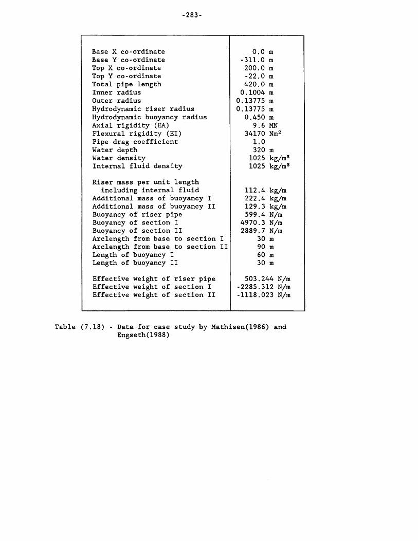
-283-

Base X co-ordinate 0.0 mBase Y co-ordinate -311.0 mTop X co-ordinate 200.0 mTop Y co-ordinate -22.0 mTotal pipe length 420.0 mInner radius 0.1004 mOuter radius 0.13775 mHydrodynamic riser radius 0.13775 mHydrodynamic buoyancy radius 0.450 mAxial rigidity (EA) 9.6 MNFlexural rigidity (El) 34170 Nm2Pipe drag coefficient 1.0Water depth 320 mWater density 1025 kg/m3Internal fluid density 1025 kg/m3

Riser mass per unit lengthincluding internal fluid 112.4 kg/m

Additional mass of buoyancy I 222.4 kg/mAdditional mass of buoyancy II 129.3 kg/mBuoyancy of riser pipe 599.4 N/mBuoyancy of section I 4970.3 N/mBuoyancy of section II 2889.7 N/mArclength from base to section I 30 mArclength from base to section II 90 mLength of buoyancy I 60 mLength of buoyancy II 30 m

Effective weight of riser pipe 503.244 N/mEffective weight of section I -2285.312 N/mEffective weight of section II -1118.023 N/m

Table (7.18) - Data for case study by Mathisen(1986) and Engseth(1988)

-284-

Total length of pipe 3004 mSeparation between vessels 3000 mInner radius of pipe 0.325 mOuter radius of pipe 0.335 mWave height 5 mWave period 12 sWave length 224 mDepth of water 110 mDepth to sled 10 mMass of sleds at pipe ends 0 tonnesEffective weight per unit length 20 NEnd tension (No current) 327700 N

Table (7.19) - Data for towed pipeline analysis

- 285 -

Buoy Geometry in Heriot-Watt M odel Tests

M odel Buoy 3.9" O.D.<j

Flexible Pipe

L Model Saddle 5" diameter at pipe CL

Distance between centres of buoy and saddle = 3.69"

Figure 7.1 - Buoy Geometry in Heriot-Watt Model Tests

Ver

tical

Pro

ject

ion

(m)

- 286-

3.000

2.000

1.000

0.000-1.000 1.0000.000 2.000

Horizontal Projection (m)

- LEGEND -+ Heriot-Watt Model Tests

0 Heriot-Watt Monitored Points

REFLEX

Figure 7.2 - Comparison of staticprofiles from Heriot-Watt model tests

and REFLEX (Fixed Top)

Ver

tical

Pro

ject

ion

(m)

- 287 -

3.000

2.000

1.000

0.0002.0000.000 1.000- 1.000


- LEGEND - Static Profile Dynamic Minimum Dynamic Maximum

H = 0.127m, T = 1.130s

Figure 7.3 - Comparison of dynamicdisplacements from Heriot-Watt model

test 1 and REFLEX

Ver

tical

Pro

ject

ion

(m)

- 288 -

3.000

2.000

1.000

0.0001.000 2.000-1.000 0.000


- LEGEND - Static Profile

Dynamic Minimum

Dynamic Maximum

H = 0.127m, T= 1.414s


test 2 and REFLEX

Ver

tical

Pro

ject

ion

(m)

- 289 -

3.000

2.000

1.000

0 . 0 0 0 -

2.0001.0000.000-1.000



H = 0.127m, T = 1.695s


test 3 and REFLEX

Ver

tical

Pro

ject

ion

(m)

3.000

2.000

1.000

0.000 -2.0000.000-1.000 1.000



Dynamic Minimum

Dynamic Maximum

H = 0.127m, T = 1.980s


test 4 and REFLEX

Ver

tical

Pro

ject

ion

(m)

- 291 -

3.000

2.000

1.000

0.0000.000-1.000 1.000 2.000


- LEGEND - Static Profile Dynamic Minimum

Dynamic Maximum

H = 0.127m, T = 2.273s


test 5 and REFLEX

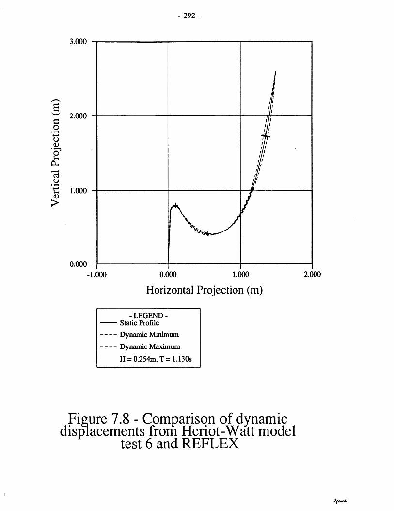
Ver

tical

Pro

ject

ion

(m)

- 2 9 2 -

3.000

2.000

1.000

0.0002.0000.000 1.000-1.000



Dynamic Maximum

H = 0.254m, T = 1.130s


test 6 and REFLEX

Ver

tical

Pro

ject

ion

(m)

- 293 -

3.000

2.000

1.000

0.000 -2.0001.0000.000-1.000



Dynamic Maximum

H = 0.254m, T = 1.414s


test 7 and REFLEX

Ver

tical

Pro

ject

ion

(m)

- 294 -

3.000

2.000

1.000

0.0001.000 2.000-1.000 0.000



Dynamic Minimum

Dynamic Maximum

H = 0.254m, T= 1.695s


test 8 and REFLEX

hptwnL

Ver

tical

Pro

ject

ion

(m)

- 295 -

3.000

2.000

1.000

0.000 -2.0001.0000.000-1.000



Dynamic Minimum

Dynamic Maximum

H = 0.254, T = 1.980s

Figure 7.11 - Comparison of dynamicdisplacements from Heriot-Waft model

test 9 and REFLEX

&pumt

Ver

tical

Pro

ject

ion

(m)

- 29 6 -

3.000

2.000

1.000

0.0000.000-1.000 1.000 2.000



Dynamic Minimum

Dynamic Maximum

H = 0.254m, T = 2.273s


test 10 and REFLEX

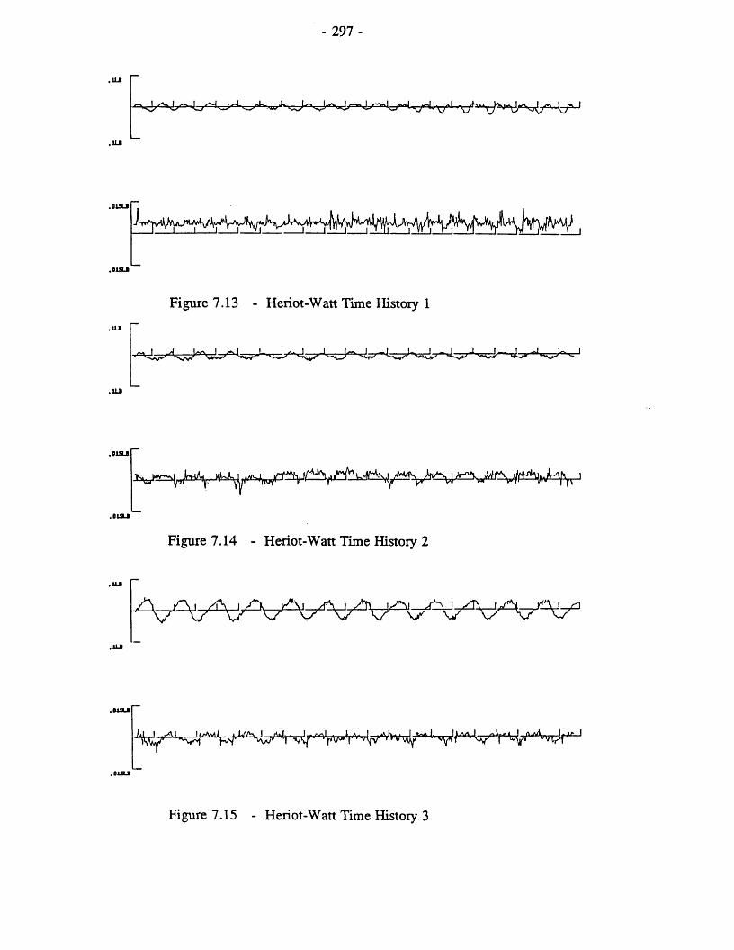
Figure 7.13 - Heriot-Watt Time History 1


j A\ i / , k yc\i ..vf\ i


- 298

.1LS

J-wjAfy.! 1V


• UJ

Vl


,1LI

L


299


J*


- 300 -


1LB


Ver

tical

Pro

ject

ion

(m)

- 301 -

3.000

2.000

1.000

0.000 -2.5001.5000.500-0.500


- LEGEND -+ Heriot-Watt Model Tests

o Heriot-Watt Monitored Points

- REFLEX

Figure 7.23 - Comparison of staticprofiles from Heriot-Watt model tests

and REFLEX (Vessel Motion)

Ver

tical

Pro

ject

ion

(m)

- 302-

3.000

2.000

1.000

0.000 -1.500 2.5000.500-0.500



Dynamic Maximum

H = 0.12m, T = 1.414s


test V-l and REFLEX

Ver

tical

Pro

ject

ion

(m)

- 303 -

3.000

2.000

1.000

0.000 -2.5001.500-0.500 0.500



H = 0.12m, T = 1.695s


test V-2 and REFLEX

Ver

tical

Pro

ject

ion

(m)

- 304-

3.000

2.000

1.000

0.0002.500-0.500 0.500 1.500



Dynamic Maximum

H = 0.12m, T = 1.980s


test V-3 and REFLEX

Ver

tical

Pro

ject

ion

(m)

- 305 -

3.000

2.000

1.000

0.000 -2.5001.5000.500-0.500



Dynamic Minimum

Dynamic Maximum

H = 0.12m, T = 2.273s


test V-4 and REFLEX

hp*i/n£

Ver

tical

Pro

ject

ion

(m)

- 306-

3.000

2.000

1.000

0.0002.500-0.500 0.500 1.500



Dynamic Minimum

Dynamic Maximum

H = 0.24m, T = 1.414s


test V-5 and REFLEX

Ver

tical

Pro

ject

ion

(m)

- 307 -

3.000

2.000

1.000

0.0000.500-0.500 1.500 2.500



Dynamic Minimum

Dynamic Maximum

H = 0.24m, T = 1.695s


test V-6 and REFLEX

Ver

tical

Pro

ject

ion

(m)

- 308 -

3.000

2.000

1.000

0.000-0.500 0.500 1.500 2.500



Dynamic Minimum

Dynamic Maximum

H = 0.24m, T= 1.980s


test V-7 and REFLEX J

Ver

tical

Pro

ject

ion

(m)

- 309 -

3.000

2.000

1.000

0.000-0.500 0.500 1.500 2.500



Dynamic Minimum

Dynamic Maximum

H = 0.24m, T = 2.273s


test V-8 and REFLEX

urve

SURGE

. HEAVE

TOP

WOVE

SURGE

IIERVE

- 310 -

-A— / \ i / V.— / i \ 1/ M— Lx LJ.— U— /.la— U— Xi— t-a

i i » » » -i i <__ i__ i.. i-- 1-- 1-- 1 1 . i i i__ I—, i — i

» «■ I ai - a • • *** 1 Jj ip-

Figure 7.32 - Heriot-Watt Time History V -l

, J—

Figure 7.33 - Heriot-Watt Time History V-2

- 311 -

urve

SURGE

HERVE

TOP

URVE

SURGE

IIERVE

. t i l



■la

unve

■la

9la

surge

31 a

■la

HERVE

■la

.til


URVE

SURGE

HERVE


- 313 -

Urve

SUROE

HERVE

TOP

URVE

SURGE

HERVE

R \ / \ A . A , A A A A , .. A , A , /t \ y v \ y X y 'J \ J \ J \ j \ J \ J

A J a V a \| h li ii li h lj---h — 11---Zj— \ x--La— Vi— Zl.

. i l l


k

U — U--1- / i-4—i— U — Vi--L \ — lA— 1-7 i --\ i-- U — b-- >/--1\_ i

-A---*—/— lA— »■■ / i \ i a M 4-- 4-- i /■ i \ i— /-i— X-i U — A-1-

i_l— i_l— i / i \ i A ^--- 1/-- ii---1. / i \ i— Aa— la.

. h i


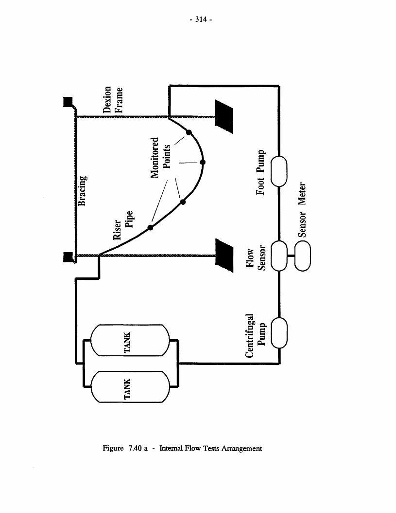
Xxo>o>

Im©C/iaOJc/d

A r\

vJ LJ

egW> a .

SS3 S x- 3c ft*o>U y

Figure 7.40 a - Internal Flow Tests Arrangement

- 315 -

carriage motion

constanttensionsprings

carriage

IL motion cam era —

glassviewingpanel

a ccessdoor

underwatertransversemotioncam era

baseconnector

vertical actuator rtop connecting platform

carnageglassviewingpanel

door

''•horiz.actuator

4.5 m

(Figures courtesy of Dr. G J Lyons) Figure 7.40 b - UCL Riser and Tether Tank

- 316-

1000

1.600 -

1.200

0.800

0.400

0.0000.300 2.000 2.3000.000 1.000

2.000

1.600 -

1.200 -

0.800 -

0.0001-500 2.0001.0000.000

Horizontal Projection (m) Horizontal Projection (m)

-LEGEND - Experiment (UCL)

REFLEX

_ . LEGEND -Q Experiment (UCL)

Figure 7.41 - Displaced riser profiles Figure 7.42 - Displaced riser profilesfor UCL pressure test 1 lor UCL static pressure test 2

1000

1.600

1.200 -

0.800

0.400 -

0.0000.000 OJOO 1.000

1000

1.600

1.200 -

0.800 -

0.400 -

0.0000.000 1J000.300 1.000 1000


_ -LEGEND - Experlintut (UCL)

REFLEX

_ . LEGEND - ( J Experiment (UCL) REFLEX

Figure 7.43 - Displaced riser profiles Figure 7.44 - Displaced riser profilesfor UCL static pressure test 3 for UCL static pressure test 4

- 317

1.670 -

8£Oo1H■£i>

0.680 -

0.3501.600 2.0000.400 0.800 1.2000.000


—. - LEGEND - Experiment (UCL)

2.000

1.670 -

a£Oou‘s’CL13

1.340 -

1.010Ol

0.680 -

0.3501.200 1.6000.000 0.400 0.800 2.000


„ - LEGEND-Experiment (UCL)

REFLEX

Figure 7.45 - Displaced riser profiles for UCL static pressure test 5

Figure 7.46 - Displaced riser profiles for UCL static pressure test 6

4.500

4.000 -

3.500 -

2.0000.300 0.600 0.900 1.2000.000


4.500

4.000 -

ac

. § 3.500 -o .*>i’tS 3.000 -

I2JOO -

2.0000.000 0.300 0.600 1.2000.900


- LEGEND - - LEGEND -------REFLEX ------REFLEXQ Experiment (UCL) Experiment (UCL)

Figure 7.47 - Displaced riser profilesFor UCL riser tank pressure test 1

Figure 7.48 - Displaced riser profiles For UCL riser tank pressure test 2

- 318

2.000

1.670 -

Eco

0.6*0 -

0.3501.200 1.600 2.0000.000 0.400 O.SOO


2.000

1.670 -

Ec.2 1.340 -

!"3 1.010 -oV>

0.6*0 -

0.3500.(00 1.600 2.0000.000 0.400


• LEGEND - • LEGEND ------ REFLEX ------REFLEXQ Experiment (UCL) Q Experiment (UCL)

Figure 7.49 - Displaced riser profiles for UCL internal ilow test 1

Figure 7.50 - Displaced riser profiles for UCL internal flow test 2

2.000

1.670 -

0.6*0 -

0.3500.000 0.400 0.100 1.200 1.600 2.000


2.000

0.6*0 -

0.3500.000 0.400 0.800 1.600 2.000


-LEGEND• -LEGEND •------REFLEX ------REFLEXQ Experiment (UCL) Q Experiment

Figure 7.51 - Displaced riser profilesfor UCL internal flow test 3

Figure 7.52 - Displaced riser profiles for UCL internal flow test 4

ipfunt

- 319-

4.500

4.000 -

✓—.

I3.000

u>2.500 -

2.0000.300 0.6000.000 0.900 1.200

4.000 -

3.500 -

10001.5001.2000.600 0.9000.000 0.300


- LEGEND - REFLEX

Experiment (UCL)

- LEGEND - REFLEXQ Experiment (UCL)

Figure 7.53- Displaced riser profiles for U CL riser tank internal flow test 1

2.000

1.670 -

1.340 -

TJ 1.010 -

0.680 -

0.3501.200 1.600 2.0000.000 0.400 0.800


Figure 7.54 - Displaced riser profiles for UCL riser tank internal flow test 2

2.000

1.660 -

Be.2 1.320 -6 .o

1*3 0.980

'S£

0.640 -

0.3000.000 0.400 0.800 1.200 1.600 2.000


- LEGEND - - LEGEND-------REFLEX bound* ------REFLEX Bound*Q Experimeul Bound* Experiment Bound*

Figure 7.55 - Comparison of dynamicdisplacements for UCL internal flow

test 1

Figure 7.56 - Comparison of dynamicdisplacements for UCL internal flow

test 2

hp/wni

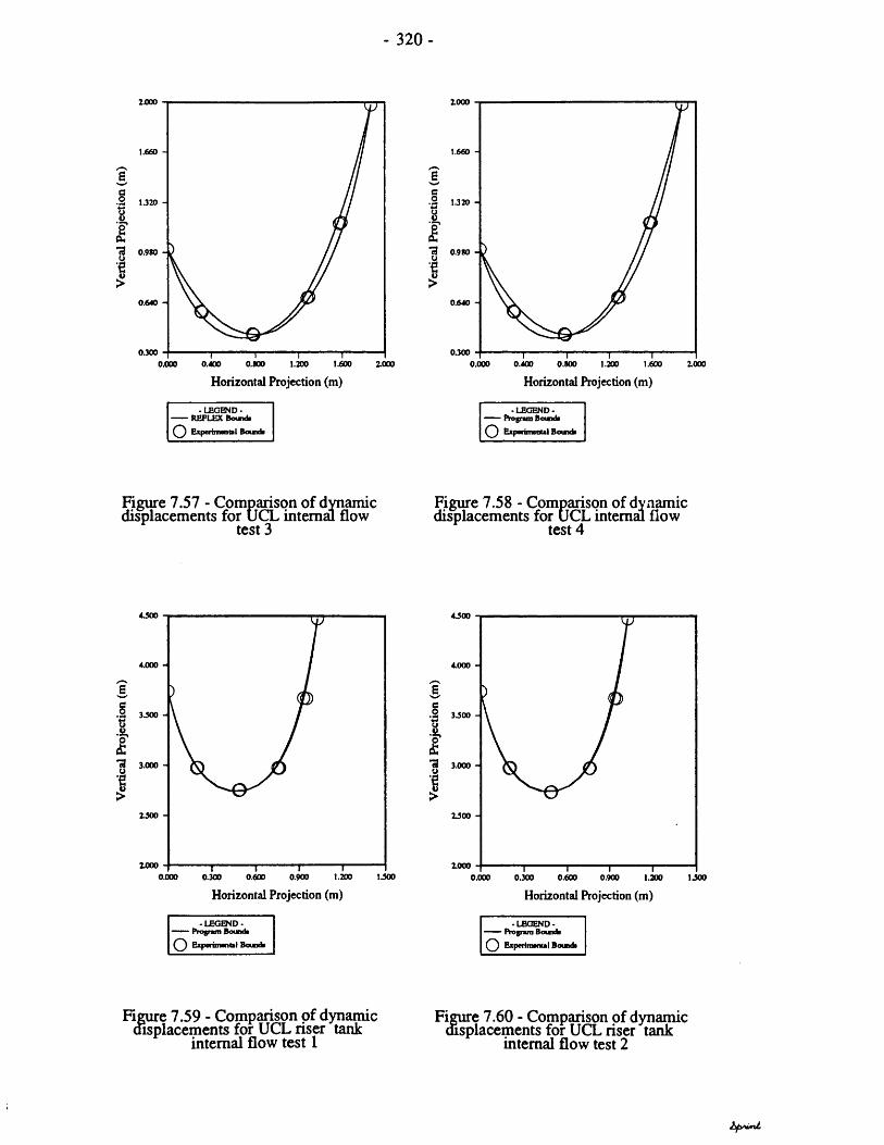
- 320-

2.000

1.660 -

Ea0t>u1au•fi£

1.320 -

0.9*0

0.640 -

0.3001.6000.000 0.400 0.800 1.200 2.000


1000

1.660 -

Bco0 V1■a

t.320 -

0.980UI

0.640 -

0.3001.600 10000.000 0.400 0.800 1.200


- LEGEND - - LEGEND -------REFLEX Bowxfa — Program BowlsQ Experimental Bounds Q Experimental Bouide

Figure 7.57 - Comparison of dynamic displacements for UCL internal flow

test 3Figure 7.58 - Comparison of dynamic displacements for UCL internal flow

test 4

4.000 -

E

!"3 3.000 -

I1300 -

10001.200 1.5000.000 0.300 0.600 0.900


4.000 -

/—sE

10000.000 0.300 1.2000.900


■ LEGEND• . LEGEND-— Program Bounds .......Program BoundsQ Experimmtal Botnds Q Experimental Bomds

Figure 7.59 - Comparison of dynamicdisplacements for UCL riser tank

internal flow test 1Figure 7.60 - Comparison of dynamic

displacements for UCL riser tankinternal flow test 2

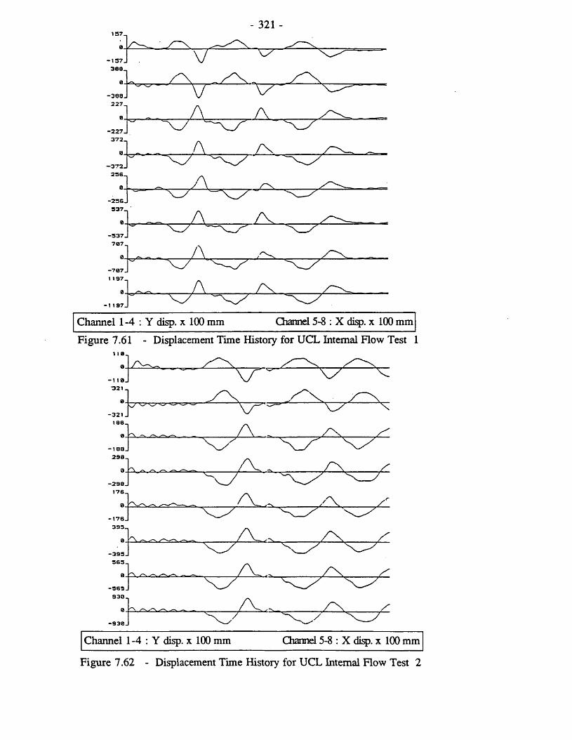
- 321 -137e

-157 J 3 8 8 -

-3 0 8 J

VA _ / \

V '“X T '227 —

2S6_

0 A-25 S j 337-,

-337707_

A . A .

-707 . 1 197.

0.

■11 97.

A

A A

Channel 1 -4 : Y disp. x 100 mm Channel 5-8 : X disp. x 100 mm

Figure 7.61 - Displacement Time History for UCL Internal Flow Test 1110 . ,

0- 1 10J 321

\ A

-321 J 188-

\

/ X— 188 J

298.,

A / V—298J

176 —

A

-176 .393.

A

A-393 J 363-,

-3 6 3930.

0-9 3 0 .

A / V a :

A/

Channel 1 -4 : Y disp. x 100 mm Channel 5-8 : X disp. x 100 mm

Figure 7.62 - Displacement Time History for UCL Internal Flow Test 2

322

33C.220.

220_

A / \- \ J -N

Channel 1-4 : Y disp. x 100 mm Channel 5-8 : X disp. x 100 mm

Figure 7.63 - Displacement Time History for UCL Internal Flow Test 31 17-

Channel 1-4 : Y disp. x 100 mm Channel 5-8 : X disp. x 100 mm

Figure 7.64 - Displacement Time History for UCL Internal Flow Test 4

- I195_

Channel l -4 : Y disp. x 100 mm Channel 5-8 : X disp. x 100 mm

Figure 7.65 - Displacement Time History for UCL Riser Tank Internal Row Test l

Channel l -4 : Y disp. x 100 mm Channel 5-8 : X disp. x 100 mm

Figure 7.66 - Displacement Time History for UCL Riser Tank Internal Flow Test 2

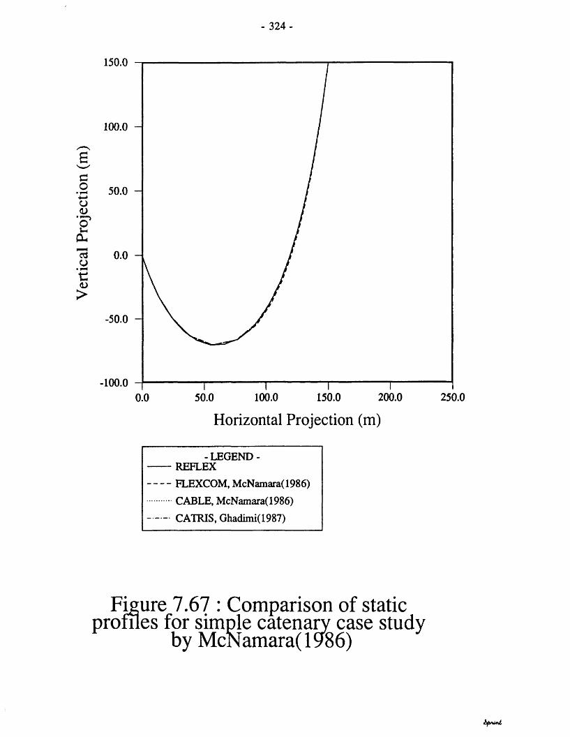
Ver

tical

Pro

ject

ion

(m)

- 324 -

150.0

100.0

50.0

0.0

-50.0

-100.00.0 50.0 100.0 150.0 200.0


250.0

- LEGEND - REFLEX

FLEXCOM, McNamara( 1986) CABLE, McNamara(1986) CATRIS, Ghadimi(1987)

Figure 7.67 : Comparison of static profiles for simple catenary case study

by McNamara( 1986)

Tens

ile

Forc

e (N

)

- 325 -

xlO3100.0

70.0 -

40.0

10.0 -

-20.0 -

-50.0350.0280.00.0 70.0 140.0 210.0

Arclength (m)

- LEGEND REFLEX

FLEXCOM, McNamara(1986)CABLE, McNamara(1986)

CATRIS, Ghadimi(1987)

Figure 7.68 : Comparison of static tensile forces for simple catenary case

study by McNamara(1986)

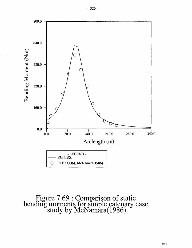
Bend

ing

Mom

ent

(Nm

)

- 326 -

800.0

640.0

480.0

320.0

160.0

0.00.0 70.0 140.0 210.0 280.0 350.0

Arclength (m)

- LEGEND - REFLEXO FLEXCOM, McNamara( 1986)

Figure 7.69 : Comparison of staticbending moments for simple catenary case

study by McNamara(1986)

ipswnl

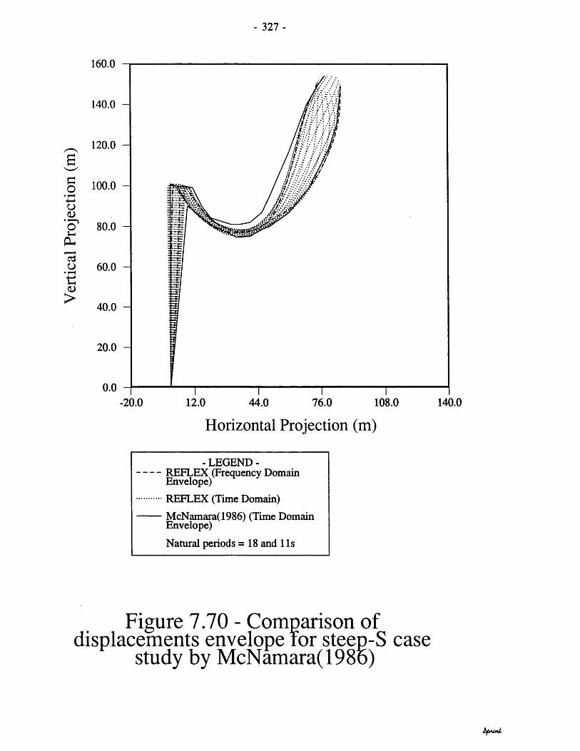
Ver

tical

Pro

ject

ion

(m)

- 327 -

160.0

140.0 -

120.0 -

100.0 -

80.0 -

60.0 -

40.0 -

20.0 -

0.044.0 140.0-20.0 12.0 76.0 108.0


- LEGEND - REFLEX (Frequency Domain

Envelope) REFLEX (Time Domain) McNamara(1986) (Time Domain

Envelope)Natural periods = 18 and 1 Is

Figure 7.70 - Comparison ofdisplacements envelope tor steep-S case

study by McNamara(198o)

Bend

ing

Mom

ent

(kN

m)

- 328 -

WAVE LOADS AND VESSEL MOTIONS

0AO

E-0.72

z'0.88

9 7 8 0 9 8 2 0 986.0 9900 9 9 4 0 9 9 8 0 KX3ZO 10060 10)00 10(40 10(80TIME (SECS.)

FIG, 17 BENDING MOMENT AT NOPE 17 DUE TO WAVES

-0.40

1.72

I.8S

1.04

-1.20

•1.3624.0 32.0 36.00.0 8.0 48.0 64.040.0

Time (s)

- LEGEND•REFLEX ( T in Domain)McNimar^l986) boundsArclensth ■ 143m H*20m T * 16sTime step « 023s

Figure 7.71 - Comparison of bending moment variations for steep-S case study

by McNamara(1986)

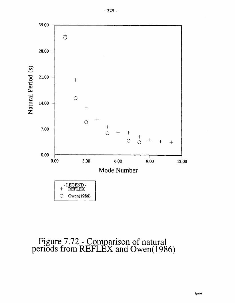
Nat

ural

Per

iod

(s)

- 329 -

35.00 -i

28.00 -

21.00 -

14.00 -

7.00 -

0.000.00 3.00 6.00 9.00 12.00

Mode Number

- L E G E N D - 4- REFLEXO Owen(1986)

Figure 7.72 - Comparison of naturalperiods from REFLEX and Owen(1986)

Ver

tical

Pro

ject

ion

(m)

- 330 -

HOOELs STAncOtSPLACEflENTS

: UNDER CURRENT . .794( 3 . 8

100aSVL

no c u rre n t

100

100.0

70.0

40.0

10.0

-40.0 20.0 S0.0 140.0


- LEGEND - ------------- No C u ra t— — — — C utra t ♦ Vm m I Excuntca

Uf-50) - OS nVbu;t 30J - 0 J u(ia))- ij

Figure 7.73 - Comparison of geometriesfor Owen(1986) case study with current

and vessel excursion

Ver

tical

Pro

ject

ion

(m)

- 331 -

WT7M. miJHH

tWVT hf/OfT ■ If m

lsnctk in peter

100.0

70.0

40.0

10.0

•20.0

-50.080.0 140.020.0 200.0•100.0 •40.0

- LEGEND - Sutic Profile


— — — — Displacement faivelopo

REFLEX reiultf for H e|6m , T“ 12» wave

Figure 7.74 - Comparison ofdisplacements envelope for Owen(1986)

without vessel motions

Ver

tical

Pro

ject

ion

(m)

X I# 1•U- 332 -

fNtrtAL rosirioN e.e.t.¥4 ye pe*/ao * /* s ¥4 ye tff&tr * it m rtaoei resr i noon. // j yA ye *e*rao • t* *¥4 ye tf/GHr * 15 m

LENGTH IN f tT fB

-€ -5 -4 -3 -2 -I • I 2 3 « 5 6 7 8 9 18 IIX I81

110.0

71.0

46.0

14.0

-11.0

-30.0 20.0 10.0 140.0 200.0•100.0Horizontal Projection (m)

-LEGEND- ------------- Stttic ProfiJr— — — — DfopUcamrat &iv«lop»

REFLEX r**uJu far H“ l6m , T-12* w»*«

Figure 7.75 - Comparison ofdisplacements envelope for Owen(1986)

with vessel motions

M

Ver

tical

Pro

ject

ion

(m)

- 333 -

350.0

280.0

210.0

140.0

70.0

0.00.0 70.0 140.0 280.0210.0 350.0


- LEGEND - REFLEX (Intermediate) REFLEX (Final)+ 0 ’Brien(1988)

Figure 7.76 - Comparison of in-planeprofiles with O’Brien (1988)

Ver

tical

Pro

ject

ion

(m)

- 334 -

400.0

300.0 -

200.0 -

'i ' i

100.0 -

0.0 -20.00 30.000.00 10.00-10.00

Out of Plane Projection (m)

- LEGEND - REFLEX (Tensile+Geometric

Non-linearity) REFLEX (Geometric

Non-linearity)+ 0 ’Brien(1988)

Figure 7.77 - Comparison of out of plane profiles under cross current with

O’Brien (1988)

Wal

l Te

nsio

n (N

)

- 335 -

xlO3500.0

300.0

100.0

500.00.0 100.0 200.0 300.0 400.0

Arclength (m)

- LEGEND - REFLEX (No Current) REFLEX (Cross Current) 0 ’Brien(1988) (No Current)

+ 0 ’Brien(1988) (Cross Current)REFLEX (Effective Tension,No Current)

Figure 7.78 - Comparison of tensile forces with O Brien (1988)

Bend

ing

Mom

ent

(Nm

)

- 336 -

xlO33.000

2.000

1.000

0.000

-1.000

-2.000

-3.000500.0300.0 400.0100.0 200.00.0

Arclength (m)

- LEGEND - REFLEX (No Current) REFLEX (Cross Current)

+ 0 ’Brien(1988) (No Current)O 0 ’Brien(1988) (Cross Current)

Figure 7.79 - Comparison of bendingmoments with O’Brien (1988)

Out

of

Plan

e Be

ndin

g M

omen

t (N

m)

- 337 -

3.000

2.000 -

1.000 -

,000

-1.000 -

-2.000 -

-3.000500.00.0 100.0 200.0 300.0 400.0

Arclength (m)

- LEGEND - REFLEX (Cross Current)+ 0 ’Brien(1988) (Cross Current)

Figure 7.80 - Comparison of out ofplane bending moments with O’Brien

(1988)

hft/vuni

Torq

ue

(Nm

)

- 338 -

5.000

4.000 -

3.000 -

2.000 -

1.000 -

0.000 -

-1.000 -

-2.000300.0 400.00.0 100.0 200.0 500.0

Arclength (m)

- LEGEND- REFLEX (Cross Current)

Figure 7.81 - Riser torques for case study by 0 ’Brien(1988)

Ver

tical

Pro

ject

ion

(m)

- 339 -

0.0

■66.7

133.3

200.0

266.7

■333.3

-400.0280.00.0 70.0 140.0 210.0 350.0 420.0


- LEGEND - REFLEX (Intermediate) REFLEX (Final)4- Mathisen(1986), Engseth(1988)

Figure 7.82 - Incremental shifting for calculation of static profile due to

Mathisen(1986) and Engseth(1988)

Ver

tical

Pro

ject

ion

(m)

- 340-

0.0

-70.0 -

-140.0 -

-210.0 -

-280.0 -

-350.0 -230.0 300.0160.090.020.0-50.0


- LEGEND - REFLEX (Multiple catenary)4- Mathisen(1986), Engseth(1988)

Figure 7.83 - Comparison of multiple catenary solution for static profile

with Mathisen(1986) and Engseth(1988)

Eff

ectiv

e Te

nsio

n (N

)

- 341 -

xlO3200.0

150.0

100.0

50.0

0.070.0 140.0 210.00.0 280.0 350.0 420.0

Arclength (m)

- LEGEND - REFLEX+ Engseth(1988)

Figure 7.84 - Comparison of effective tensions with Tingseth( 1988)

hpSwnL

Bend

ing

Mom

ent

(Nm

)

- 342 -

xlO32.000

1 . 0 0 0 -

0.000

-1.000 -

-2.000 -

450.0225.0 375.00.0 75.0 150.0 300.0

Arclength (m)

- LEGEND - REFLEX4- Engseth(1988)

Figure 7.85 - Comparison of bendingmoments with Engseth(1988)

Nat

ural

Fre

quen

cy

(Hz)

- 343 -

0.20

0.16

0.12

0.08

0.04

0.0035.020.0 25.0 30.00.0 5.0 10.0 15.0

Mode Number

- LEGEND - REFLEX Anti-symmetric modes from

simplified theory Symmetric modes from

simplified theory

Figure 7.86 - Natural frequencies of vibration for towed pipeline case study

- 344-

2.4

6,

aI| »§iaT3 -1.2 uts:>

\/ \/ \/

-2.41.000 2.000 3.0000.000


-LEGEND - REFLEX (100 .Uoirou)

----------------------------- toory

*10*

Figure 7.87 - Dynamic vertical displacements for towed pipeline case

study

400.0

o.0.0

00[200.0

-400.01.000 3.0000.000 2.000


- LEGEND - REFLEX (I00«l«ranu)

— — SbrpBfwd dxory

ilOJ

Figure 7.88 - Bending moment variations for towed pipeline case study

- 345 -

0.80

0.60 -

CT 0.40 -

0.20 -

0.00 -

10.0. 20. 30. 40. 50.

Mode Number

- LEGEND - Symmetric modes Anti-symmetric modes

from simplified method

Figure 7.89 - Modal participation parameters for towed pipeline case study

-346-

CHAPTER 8 : APPLICATION STUDIES

8.1 - Introduction

This chapter illustrates the application of the numerical and theoretical techniques whose development and verification was discussed earlier in this work. Several case studies are presented to show aspects of flexible riser performance and design that have received little of no attention in the literature but are deemed to be of significance. Firstly, the analytical methods developed in chapter 4 are used to carry out a study of the motion senitivity of different flexible riser geometries to changes in parameters such as horizontal separation, buoyancy position and buoyancy magnitude. These are then followed by an examination of the contribution of vessel motions in surge and heave to total flexible riser response. The governing assumption in most linear frequency and time domain techniques is that the riser natural frequencies, calculated about the static equilibrium geometry, are invariant during loading. A study of natural frequencies of steep-S and lazy-S geometries is presented which shows natural frequencies to have different sensitivities to each geometric variable.

Several aspects of static analysis of flexible risers are considered in this chapter. Firstly, the well publicised problem of numerical instability in finite element analysis of flexible risers is illustrated by comparison of results obtained for two different pipe flexural rigidities using identical numerical procedures. A comparison of different non-linear methods for calculation of pipe static geometry is carried out to investigate the relative significance of different sources of non-linearity. The response of a lazy-wave riser to a steady current at different incidence angles is then studied and it is illustrated that out of plane loading on flexible risers is predominantly resisted by a tensile force redistribution in a manner analogous to a pendulum subjected to a steady horizontal force.

Dynamic riser response calculations in the frequency domain using a superposition of the static and dynamic responses is then compared to those obtained using the combined linearisation discussed in

-347-

Chapter 6. The importance and range of validity of each technique is illustrated. This is followed by an illustartion of the equivalance of the frequency and time domain approaches in calculation of the dynamic response followed by an assessment of the relative merits of frequency and time domain techniques. Example results from the time domain analysis program are then presented which examine the influence of wave incidence angle on riser displacements and forces. The response of the riser to an irregular, in-plane sea-state is then examined. The problem of seabed contact is next studied using a lazy-wave riser in a moderate water depth and differences between fixed and variable seabed contact models is illustrated. The final section of the chapter provides an examination of the effect of internal flow on the dynamics of a flexible riser of a lazy-S configuration. Five wave frequencies are considered with a typical extreme internal flow condition to show the strongly non-linear interaction between external and internal loadings on production flowlines.

-348-

8.2 - APPLICATION STUDIES

8.2.1 - Selection of Buov Upthrust

The choice of buoy upthrust has a direct bearing on the dynamics of a flexible riser system. A buoy near the surface may be subjected to excessive wave loading whilst one at a large depth will increase the tensioning requirements of the support vessel as well as leaving a larger length of pipe in the wave penetration zone. A study of this phenomenon will involve a large number of parameters whose relative contribution to the dynamics of the pipe depend on the particulars of the location studied. An approximate picture may be composed through a quasi-static investigation of the motion sensitivity of riser geometries using the analytical approach suggested in Chapter 4. For the pipe of properties listed in Table(8.1) at a constant water depth of 350 metres, vessel surge and heave motions of 10m amplitude are applied quasi-statically.

Four different geometries are considered, namely; steep-S, steep-wave, lazy-S and lazy-wave. The resulting envelopes of motions are presented in Figures (8.1) to (8.4).The buoyancy here is varied in proportion to the total buoyant pipe weight and is denoted by the ratio (T/W) where T is the total buoyancy and W the total buoyant weight of the pipe. The steep-S geometry in Figure(8.1) show that for the same set of vessel motions, the pipe with the higher buoyancy provision (T/W-2.0) experiences lesser oscillations of the lower limb. Bending oscillations at the sagbend region generally seem unaffected. Although the increase in the buoyancy will inevitably increase the tensile forces in the lower limb. These tensions serve to reduce the angle to the vertical ofthe lower limb and hence the bending moments at its bottomconnection. An increase in the buoyancy will also be expected toreduce the range of dynamic rotations at the base connection. Ahigher buoy upthrust is likely to lower the natural periods of the pipe towards the wave excitation region. However, since in most case the natural frequencies of the pipe are well above those of dominant wave periods, the first natural periods will still remain well above the wave periods. The natural periods of the steep-S riser are presented later in this chapter and are shown to lie

-349-

typically in the 40 to 60 seconds range.

The steep-wave risers shown in Figure (8.2) show a more pronounced change in their geometry with variations of buoyancy. Firstly, a lifting of the buoyancy arch is noted which now in absence of the buoy will also lead to a reduction in the bending radius at the arch. Bending at the sagbend is still unaffected but the same is shown to increase significantly at the lower connection. Comparison with the steep-S case also shows an increase in sagbend motion envelope. Bending oscillations at the seabed, which are known to result in large snap loads are avoided with this geometry. This forces a restriction on the minimum buoyancy provision for the pipe. In general, design ensures that for all possible pipe internal fluid densities, the lower connection retains a minimum tension level. Identification of the minimum buoyancy may be carried out very simply using the analytical approach used here which is likely to take minutes compared to the finite element models requiring many hours to examine several geometries and effective weights.

The lazy-S riser shown in Figure (8.3) behaves analogously to the steep-S geometry with the exception that due to the difference in the geometry, the minumum buoyancy required to support the pipe is larger. For this reason the lowest buoyancy studied has been increased to (T/W=1.0). The buoy in this geometry helps with the absorption of the dynamic horizontal tension fluctuations effected by the upper pipe and allows little to be transmitted to the lower pipe. As seen, motions of the lower limb due to the upper pipe are practically eliminated for (T/W>1.5). Typical natural frequencies of this geometry range between 30 and 60 seconds and since the buoy merely acts as an intermediate support, increasing the buoyancy will stabilise the system further without an appreciable change of its natural frequencies.

Analysis of the lazy-wave geometries in Figure (8.4) revealed major disadvantages in their use for some offshore applications. The geometries presented show this riser to be extremely sensitive to changes in the buoyancy. As seen on the Figure buoyancy could only be varied within (0.4<T/W<0.6) which is very restrictive. Further,

-350-

for these changes in buoyancy, the length resting on the seabed varied from 10 to 75 metres which is clearly unacceptable in any design case. The vessel motions also resulted in moderately large movements in the seabed lift-off point (approx. 10 metres). The extreme sensitivity of this geometry to the magnitude of buoyancy provision was investigated further by calculating the geometry of the lazy-wave with different internal fluid densities. The results in Figure (8.5) show very large changes in geometry for approxiomately 10% changes in internal fluid density. This implies that an internal flow of time varying density is likely to set this geometry into large oscillation, given that a typical two-phase flow can exhibit time dependent changes in density of up to 50% of mean.

8.2.2 - Selection of Buov Height

The depth at which the subsea buoy (or buoyancy collar) is placed is partially governed by the maximum-wave penetration depth. This is the depth at which wave excitation reduces to a given small percentage of its maximum value at the surface. This may be determined easily from the linear wave theory. For larger water depths, the buoy is often placed below 30 metres and well away from the wave excitation zone. In shallow water, other criteria must be considered in tandem and often simple catenary profiles will suffice. Other parameters affecting the choice of buoy heightinclude the surface vessel tensioning capacity, water depth, vessel offset and the choice of geometry. To provide a consistent basis for comparison, the total length of pipe is kept constant in all cases. Figures (8.6) to (8.8) show the effects of buoy height on the flexible riser geometries studied.

The steep-S riser in Figure (8.6) shows little change in its quasi-static displacements. Interestingly, the buoy maintains exactly the same angle to the vertical in all cases and undergoes similar rotations with vessel motions. It should be noted that the wave induced loading on the geometry with a 150m buoy height willbe greater than on the geometry with the 250m buoy due to the additional exposed length of pipe. The steep-wave riser shows anexpected axial stiffening of the lower connection caused by

-351-

lowering the buoy height. It is seen that the minimum buoyancy criterion is thus affected which in design would require a re-analysis. The sagbend motion envelope is seen to have widened in comparison with the steep-S case. The lazy-S riser, using a moderate buoyancy of (T/W-1.0) is seen to accommodate the motions with ease and little changes in its lift-off position. The lazy-wave geometry has been excluded from this study since the height of its buoyancy arch may not be controlled independently without a complete change of profile and pipe length.

Figures (8.9) to (8.11) show the effect of buoy height on the tensile forces along the pipe. The figures use a normalised scale for ease of comparison and are all drawn on the same vertical scale. It is noted from Figures (8.9) and (8.11) that changes in the buoy height serve to proportion the tensions between the vessel connection and the connection of the lower simple catenary to the buoy. These figures correspond to the steep-S and lazy-S geometries and emphasise the large gradients of tensions around the subsea buoy arch. Such rapid changes in forces are likely to have added fatigue and wear implications which are beyond the scope of this work. The steep-wave tensions in Figure (8.10) show a more uniform distribution of tensile forces and a lower global stress state. It should be noted that by reducing the buoy upthrust in the steep-S case, the tensile forces may be alleviated considerably and the presented tension distribution is not a general feature. It should also be remarked that the changes in tensile forces with vessel motions are quite small in comparison with those resulting from buoy relocation.

Figures (8.12) and (8.13) illustrate the influence of buoy positioning on the natural periods of the steep-S and lazy-S risers. Schematic plots of the first mode shape are also included in these figures. Results for the steep-wave and lazy-wave risers were observed to have the same characteristics and have, therefore, been omitted for brevity. It is seen from Figure (8.12) that only the first natural period of the steep-S riser is affected and the increase in the buoy height above the seabed has raised the first natural period leaving the lower periods unpurturbed. The change in natural periods from a buoy height of 150 to 300 metres was from 40

-352-

to 58 seconds almost 20%. The lazy-S geometry in Figure (8.13) is similarly seen to be affected in the first mode only but to a much lesser extent. The natural periods ranged from 35 to 40 seconds approximately showing much less sensitivity. This feature of lazy-S risers is of particular benefit to the designer in removing the natural period constraint from the design optimisation.

8.2.3 - Vessel offset limitations

The foregoing discussions showed that the higher natural periods of flexible riser geometries are unaffected by vertical positioning of the buoy and only the first natural period shows an appreciable sensitivity to buoy height. The same is not true of the horizontal vessel offset. It is seen in Figures (8.14) and (8.15) that increasing the horizontal offset for a given geometry, leads to an overall reduction in all natural periods of the system. This is consistent with the definition of natural period (T-27r.y(k/m)) where an increase in the offset leads to an increase in the system stiffness and hence a reduction in its compliance leading to a shift in its natural period towards the dominant wave periods.

Figure (8.14) shows a decrease of the first natural period of the steep-S riser from 50 to 38 seconds which corresponds to an increase in vessel offset from 50 to 200 metres. Figure (8.15) shows a decrease of the first natural period of the lazy-S riser from 40 to 25 seconds for the same increase in vessel offset. The effect of vessel offset changes will lead to an expected increase in inclination of the buoy to the vertical for the lazy-S and steep-S geometries and alter the geometry of the steep-wave without affecting its quasi-static performance. These results are not presented for brevity. The lazy-wave geometry showed the expected change in its geometry except that the position of the lift-off point underwent only a very small change as shown in Figure (8.16). This was a surprising result which can be explained by arguing that horizontal motions serve to alter the horizontal distribution of the pipe weight whilst leaving its vertical distribution, i.e. its potential marginally affected. As a result, the net vertical force on the seabed touch-down point remains approximately unaltered.

-353-

8.2.4 - Relative Contribution of Vessel Motions to Pipe Response

The selection of a support vessel for a floating production system incorporating flexible risers is based on its functional suitability for the intended operations as well as its motion characteristics. It is therefore of interest to examine the realtive influences of different components of vessel motion to establish whether a given component has a more pronounced influence than the other.

Figures (8.17) to (8.19) show the effects of vessel surge and heave separately and in combination. It is seen that the vessel heave is mainly absorbed in the sag bend where it results in appreciable changes to the local curvature of the pipe and small redistributions of tensile forces. Such effects, whilst causing long term wear of the pipe layers, do not possess a great deal of inertia and are therefore expected to have little influence on the combined dynamics when wave action is included. The surge on the other hand is seen to contribute to the rigid body motions of the pipe in all cases which involve large translations of the whole structure. These are expected to generate large inertia forces and structural velocities. Additionally, since fluid drag is predominant in the upper steeply inclined sections of the pipe and acts horizontally, the interaction of the vessel surge with wave induced motions is likely to be the dominant loading on the structure. Note that fluid inertia contribution is usually small for flexible risers whose slender dimensions place them in the drag dominated regime.

8.2.5 - Surface Piercing Risers

Flexible riser connection to the vessel is carried out in different ways depending on the type of vessel, its mooring configuration and the number of flowlines employed. Flexible risers connected to the pontoons are often submerged thoroughly whilst those connected to the moonpool or the deck carry an exposed freeboard section. The surface piercing section of the riser is structurally a different component to the submerged section of the pipe. This is a result of the different effective weight of this section. Often in analysis

-354-

programs, this feature is neglected and the whole pipe is assumed to be of the same effective weight. This simplification is used to allow the simple catenary equations to be used for solution of the static equilibrium equations. The calculated effective tensions are subsequently modified for the external and internal pressures to obtain the pipe wall tensions with the effect of freeboard included at this stage only.

The use of constant effective weight for surface piercing risers is clearly an approximation and the extent of the errors involved may be illustrated using the example case of the steep-wave riser discussed earlier. The riser was provided with an extra 30 metres of freeboard above the still water level and the multiple catenary procedure described in Chapter 4 was used to obtain the equilibrium profile. For the given geometry, the shape did not change significantly since the upper pipe section was nearly vertical. The tensile force and effective tension predictions in the freeboard section were, however, affected significantly. Figure (8.20) shows that these tensions are underestimated by 14% which is a large error in calculation of expected vessel tensioning requirements. These results suggest that the effect of freeboard should always be included in design and its omission would lead to unconservative results.

8.2.6 - Static Analysis Methods

It was stated in Chapters 4 and 5 that the use of multiple catenary solutions offers a most accurate and rapid means of computing the static equilibrium geometry of flexible risers. It was pointed out that the use of incremental shifting techniques is only advisable in cases where unusual geometries or discrete loading conditions exist. However, multiple catenary solutions can not be easily modified to include loading due to a general current. Drag loading must be included using one of the non-linear techniques discussed in Chapter 5. Numerical ill-conditioning problems involved with flexible riser analyses result from two sources: the high ratio of the axial to flexural stiffness of the riser pipe (EA/EI) and, the large rigid body translations and rotations in space typically arising during shifting of the pipe to equilibrium. The latter

-355-

problem is reduced for cases where an initial static profile is available and the riser needs not be shifted to equilibrium. This leaves the high (EA/EI) as the major source of ill-conditioning. Three different static analysis methods were proposed in Chapter 5, namely; the direct iteration method, the incremental analysis method, and the hybrid techniques. Without prior knowledge of the numerical behaviour of the solution, the choice of the method is not obvious. To identify the differences between these methods, three different three-dimensional programs were developed based on the theory in Chapter 5.

The first uses the direct method where the iterations are carried out for equilibrium of tensile forces. This involves a shooting approach about the mean geometry where for each estimate ofdisplacements, the tensile forces are calculated and used tore-estimate the system stiffness matrix which is then used to re-calculate the force vector. An estimate of the error is then found from the ratio of the sum of squares of residual force to total force. The geometry is only updated at the final stage after calculation of forces. The second method is based on the incremental approach where the loading is calculated for theoriginal equilibrium geometry. This is then applied in a userprescribed number of increments and the geometry and internal forces are updated at each stage. One equilibrium correction is carried out per load step. The third method uses a hybrid approach where the direct approach is employed with two levels of iterations one for tensile forces and the other for geometry. This amounts to placing the total load on the mean geometry, calculating theresulting tensile forces and displacements and computing the system stiffness matrix for the updated geometry and tensile forces. Theresidual force is then calculated as previously and the root meansquared error is used to check for convergence. Having established convergence, the total loading is re-calculated for the updated geometry and the difference with that applied to the original geometry is used to replace the total load vector and repeat the iterations. This correction constitutes an outer incremental analysis loop for the displacement dependence of loading. Theconvergence criterion for this section is the r.m.s of the ratio of the residual force to the original total force. The hybrid method

-356-

represents an exact approach where the only non-linearity excluded is that of the pipe structural properties.

To assess the differences between these methods a case study was selected using the pipe in Table (8.1). A catenary riser of 250m length with horizontal and vertical separations of 100 and 150 metres, respectively, was used. A simple geometry was deliberately selected to simplify comparison of results. A steady current of 0.5 m/s of uniform distribution with depth was applied to the riser in the direction of the positive x-axis. This case study is used todemonstrate the effects of the calculation method as well as thenumerical problems with high (EA/EI) ratios. First, the effect of the calculation method is illustrated on a pipe whose flexural stiffness is of comparable magnitude to its axial stiffness. This gives a ratio EA/EI-340 which is 1000 times that of the pipe in Table (8.1). Figures (8.21) to (8.24) show the calculated geometries, tensile forces, shear forces and bending moments respectively.

It is noted from Figure (8.21) that displacements calculated using tensile non-linearity and incremental loading, despite being close to each other, are larger than those predicted using the exact non-linear approach including geometric, tensile and loading non-linearities. Additionally, the incremental methods are seen to approach the fully non-linear version with increasing number of steps. Since the same loading has been applied on all pipes, the lower set of displacements noted with the fully non-linear method imply that this geometry resists a larger proportion of the total load through internal stressing. This stipulation is confirmed in Figure (8.22) which shows large tensile force developments throughout the pipe length. In some parts, a 5 fold increase intensile forces is observed. The validity of these results isconfirmed by:

a) the observed rises of the incremental solutions from the results with tensile non-linearity only, suggesting that with increasing number of load steps, the exact solution will be approached asymptotically,

-357-

b) the fact that the programs used were developed independently and using different internal structures rules out major programming errors,

c) the steep-S case study presented in Chapter 7 after O'Brien and McNamara(1988) which showed that by omission of geometric andloading non-linearities from REFLEX, the results of O'Brien and McNamara were recovered.

Figures (8.23) and (8.24) show the changes in shear forces and bending moments for the same loading condition. Little change from the static results are obtained from the method with tensile non-linearity seeming to be the least accurate. The discrepancy is specially large in shear forces calculated near the pipeextremities.

8.2.7 - Numerical Difficulties with Pipes of Low Flexural Rigidity

The same analysis was then repeated for the original pipe with (EA/EI-34000). All other parameters including the convergence criterion were kept constant. Figures (8.25) to (8.28) show the results of the analysis. Displacements are seen to beindistinguishably similar. Tensile forces are identical except for the incremental method with 20 steps which appears to have moved further towards the exact solution. This is expected as the pipe is known to have a predominantly cable like behaviour. A completely different picture emerges in the case of shear forces and bending moments. Figures (8.27) and (8.28) show large disagreements between the results from the different methods. It should be noted that themagnitudes of shear forces and bending moments are very small and1000 times less than those in the previous case. The observeddeviations are solely a numerical feature and are caused by the finite precision of the computer used. Reducing the tolerance proved successful in bringing the solutions together and curves similar to those in Figures (8.23) and (8.24) were obtained. Additionally, using a non-standard, quadruple precision feature of Digital Corporation Micro-VAX FORTRAN compiler as well as reducing the tolerance level, improved the rate of convergence as well as eliminating the problem. It should be noted that the existing

-358-

algorithms are implemented in double precision and the use of single precision would be guaranteed to produce numerical problems. The foregoing observations confirmed the problem to be of a numerical origin and showed that increased computational precision was one method of overcoming the difficulties. In the absence of high precision computational facilities, it would be necessary to decouple the axial degrees of freedom or use a cable type solution and calculate the bending and shear forces from the final geometry.

The loss of precision was traced within the program and was found to originate from the local rotations of the element. These rotations served to increase the curvature of the element and bring the ends closer together. These rotations have little axial strains associated with them. However, the simple beam finite element model interpreted the apparent reduction in element lengths as a net compressive strain. The large apparent compressions served to severely destabilise the algorithm through erroneous negative effective tensions in the geometric stiffness matrix. It was possible to eliminate this effect by correction of the resulting first order displacements before calculation of element forces. This was carried out in accordance with the large deflection theory and was found quite successful and accurate. The source of numerical ill-conditioning which required the use of low tolerances and high precision computation was similarly traced to the multiplications of small rotation induced axial strains by the pipe axial rigidity to calculate the axial tensile force change. This constitutes an operation between very small and very large numbers and causes the system geometric stiffness to undergo lengthy oscillations which damp out very gradually.

8.2.8 - Out of Plane Deformation under Static Current

Out of plane deformation are relatively unexplored areas in flexible riser static analysis. The small collection of results available in literature were examined in Chapter 7 and used for comparison studies. In this section, a typical steep-wave riser, whose properties are given in Table (8.2), is used to explore the effect of a steady current whose velocity is linearly increasing from zero at the seabed to 1 m/s at the surface. The current

-359-

heading is varied in 45 degrees around a full circle. Figures (8.29) to (8.31) present the envelopes of riser displacements. Note that to avoid confusion, similar line types are used to denote identical projections of geometry in each plot. Figure (8.29) shows the side view of the deflected riser profiles with Figures (8.30) and (8.31) giving the out of plane and horizontal projections.

The behaviour of the riser under a transverse current was observed to be quite similar to a pendulum where out of plane displacements are resisted by an increase in the tensile forces along the pipe. This is consistent with the expected physics of the problem and was discussed in relation to O'Brien and McNamara(1988) case study in Chapter 7. Figure (8.32) shows the envelope of tensile forces for different angles of current incidence. The results shown are of significance in showing the largest tensions to be produced by the out of plane current. This proves the necessity for considering the out of plane forcing in design of flexible risers. This aspect has often been ignored in the past. Examination of Figures (8.33) to (8.35) shows that in-plane and out of plane bending of the pipe are limited to the pipe extremities with small torsions experienced around the buoyancy arch and the sag bend.

8.2.9 - Wave and Current Superposition

The prerequisite to a frequency domain analysis is the linearisation of the non-linear drag force. For this work, the method proposed by Krolikowski and Gay(1980) was selected and a suitable translation for finite element application was developed. The non-linear behaviour of the drag force implies that results obtained using a superposition of the riser static response under current onto the dynamic wave induced component will be different from those obtained if the wave and current velocities were assumed to act as a combined dynamic load. The same riser as in Section 6 above was used to study the response of a flexible pipe subjected to a 10m, 12s regular wave with two different currents of 0.5 and 0.1 m/s velocities.

Results were obtained using both a linear superposition of an opposing static current onto the wave and a combined linearisation

-360-

approach. Envelopes of riser displacements and tensions are shown in Figures (8.36) and (8.37). It is seen that for the 0.1 m/s current velocity, the results from the superposition model agree very closely with those from the combined linearisation approach. However, a discrepancy is noted with the 0.5 m/s current where the displacements seem to show a lower mean but a higher amplitude of oscillation. The tensile forces show an opposite effect and are larger for the combined case. Note that the maximum horizontal wave velocity at the surface is 2.618 m/s. This decreases exponentially to 0.5 m/s at 60 metres below the surface and 0.1 m/s at 116 metres depth. It may be inferred that the validity of the use of superposition technique depends on the ratio of the static to dynamic fluid velocities. For low ratios, superposition may be used to good accuracy but for larger values, a combined approach should be attempted.

A second topic of interest is the influence of relative current and wave headings on the flexible pipe. A study was carried out for the same pipe geometry and wave condition but with a higher current velocity of 1 m/s. Figure (8.38) compares the displaced profiles of the riser for following and opposing currents as well as the zero current case. It is seen that the presence of an opposing current reduces the amplitude of dynamic oscillations whilst the same is enhanced by a following current. The force envelopes shown in Figure (8.39) follow the same trend. Tensile forces for the following current case are seen to show greater oscillation amplitudes than the zero current case. The opposing current values undergo only small changes. The tensile force fluctuations at the top of the riser are negligible for all cases whilst the shear forces and bending moments show large amplitude oscillations at the top connection. In general, it may be stated that the effect of an opposing current will be to damp the dynamics of the system whilst that of a following current will magnify these.

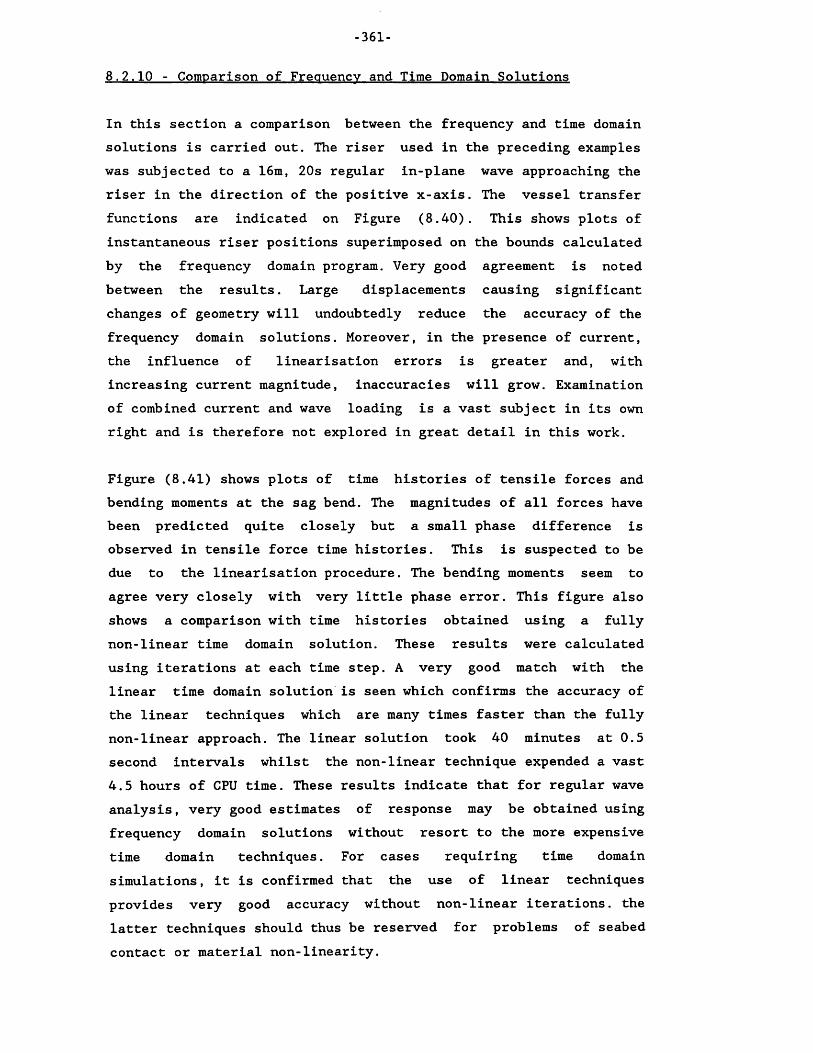
-361-

8.2.10 - Comparison of Frequency and Time Domain Solutions

In this section a comparison between the frequency and time domain solutions is carried out. The riser used in the preceding examples was subjected to a 16m, 20s regular in-plane wave approaching the riser in the direction of the positive x-axis. The vessel transfer functions are indicated on Figure (8.40). This shows plots of instantaneous riser positions superimposed on the bounds calculated by the frequency domain program. Very good agreement is noted between the results. Large displacements causing significant changes of geometry will undoubtedly reduce the accuracy of the frequency domain solutions. Moreover, in the presence of current, the influence of linearisation errors is greater and, with increasing current magnitude, inaccuracies will grow. Examination of combined current and wave loading is a vast subject in its own right and is therefore not explored in great detail in this work.

Figure (8.41) shows plots of time histories of tensile forces and bending moments at the sag bend. The magnitudes of all forces have been predicted quite closely but a small phase difference is observed in tensile force time histories. This is suspected to be due to the linearisation procedure. The bending moments seem to agree very closely with very little phase error. This figure alsoshows a comparison with time histories obtained using a fullynon-linear time domain solution. These results were calculated using iterations at each time step. A very good match with the linear time domain solution is seen which confirms the accuracy of the linear techniques which are many times faster than the fully non-linear approach. The linear solution took 40 minutes at 0.5second intervals whilst the non-linear technique expended a vast4.5 hours of CPU time. These results indicate that for regular wave analysis, very good estimates of response may be obtained using frequency domain solutions without resort to the more expensive time domain techniques. For cases requiring time domain simulations, it is confirmed that the use of linear techniques provides very good accuracy without non-linear iterations, the latter techniques should thus be reserved for problems of seabed contact or material non-linearity.

-362-

8.2.11 - Riser Response to Different Wave Headings

Riser response to different wave headings remains a sparsely addressed issue in flexible riser research. It has remained questionable whether out of plane effects are of much significance in analysis. The steep-wave geometry was selected to examine out of plane loading on these risers. To enhance the dynamics, a wave height of 20m was selected with a wave period of 16 seconds which ensured that a large wave penetration with depth was achieved. A total of 5 different wave headings were selected. Two headings were in-plane with the riser and in opposing directions whist a third was perpendicular to the vertical plane of the riser. The remaining two directions were chosen to be oblique at 45 degrees to the plane of the riser. The co-ordinate axes were defined such that the positive x-axis was horizontal along the line joining the riser base to the projection of the riser top and the y-axis was vertical. With reference to the riser geometry in Figure (8.42), the z-axis points towards the reader (out of paper). The wave angles are measured from the z-axis using the right hand screw rule such that a wave at an angle of 0 degree propagates along thez-axis whilst a 90 degree wave is directed along the positivex-axis. The riser is given a 30m freeboard over the still water level (SWL). To avoid confusing the picture vessel motions are set to zero. The simulations were carried out at 0.5 second intervals (l/32nd. of excitation period) and for a total period of 200 seconds.

Figure (8.42) shows the envelope of maximum in-plane displacements for in-plane and oblique waves. The oblique headings are clearlyseen to produce in-plane diplacements which fall within those of the 90 and -90 degrees in-plane waves. Proceeding to Figure (8.43), which shows the envelope of riser displcements out of plane, it is observed that the maximum displacements are obtained for the 0 degree wave as expected. It is noted that these envelopes areweighted in the direction of the wave propagation and that the are not symmetrical - as one might intuitively expect. It must be born in mind that the illustrated figures are envelopes and not actual riser deformation shapes. These have been calculated by scanning the time histories of displacements at each node for the largest

-363-

magnitude of out of plane displacements and noting its associated x and y value. Examination of time histories confirmed that these were zero mean but with a larger and more peaked response in the direction of wave propagation. To complete the riser displacements envelope, the plan view of the riser is shown in Figure (8.44). This shows, once again, the dominance of out of plane response to a 0 degree wave whilst illustrating the unsymmetrical nature of the oblique wave envelopes.

Figure (8.45) shows the envelopes of tensile forces for different wave headings. The in-plane response is shown to dominate, but the second largest envelope is that for a 45 degree wave heading and not the opposing in-plane wave as might have been expected. Between arclengths 330.0m and 440.0m, the situation is seen to be reversed. Moving to the torsional effects in Figure (8.46), the largest torsions are seen to be caused by the -45 degrees wave. The sagbend and archtop regions which are usually expected to suffer the greatest deal of torsion, are seen to be rivalled by the values at the SWL caused mainly by the oblique waves. This feature is of importance and provides sufficient justification for the use of out of plane analysis in dynamic design. Figure (8.47) shows the out of plane bending moment envelope for the riser. The magnitudes of bending caused by all out of plane waves seem to be quite similar with large magnifications noted at the SWL. Surprisingly this comment was seen to apply to the in-plane bending as well. It is seen in Figure (8.48) that the bending envelopes produced by in-plane waves are rivalled very closely by the out of plane and oblique waves. In selected positions, such as the top connection and the SWL, the latter are seen to dominate. These observations illustrate that out of plane loading is of significance and is capable of exciting greater responses than those induced by in-plane loadings. Whilst this single case study cannot assert a general rule, it clearly provides an example to prove the need for this type of analysis in design.

To obtain a more detailed picture of the response of the riser to different wave headings, time histories of riser moments were examined in selected areas of the pipe. These were the SWL, sagbend, arch-top and at the start of the buoyancy collar. Figures

-364-

(8.49) to (8.52) show torsion, out of plane bending moment andin-plane bending moment time histories for each position. Figure(8.49) shows the highly non-linear and impulsive nature of bending at the SWL. The torsion time history shows non-linearities with a double frequency component typical of the drag force whilst the out of plane and in-plane bending moments show higher frequencycomponents at 3 and 4 times the wave frequency. The time historiesare expectedly peaked and typical of what one might expect at the SWL region. In contrast, time histories of moments for the sag-bend show the expected double frequency component but are seen to be much smoother. Examination of Figures (8.51) and (8.52) shows the respective bending time histories for the arch-top and the start of the buoyancy collar which indicate a gradual disappearance of the double frequency component. This may be easily explained considering that the riser receives little drag or inertia loading at these depths and is merely excited by the rigid body motions ofthe upper riser which tend to be linear, periodic and at theexcitation frequency. Nevertheless, the apparent damping out of the non-linearities remains an interesting feature.

On a comparison of Figures (4.49) to (8.52) it is immediately seen that time histories in the first two figures have stabilised 40 seconds after the start of simulations whilst the torsionaloscillations in the latter two figures have taken at least twice aslong to stabilise. This effect is brought about by the low damping of torsional oscillations of the riser. Translations and flexures of the pipe receive a good deal of drag damping whilst a damping mechanism for torisonal oscillations does not exist. The time scales in Figures (8.51) and (8.52) were deliberately sliced between 40 and 120 seconds to highlight this effect.

8.2.12 - Riser Response to Irregular Sea States

The software developed in this work provides a facility for analysis of irregular sea states. Typical results are provided to exemplify the process of modelling these sea states. A JONSWAP sea state was used which corresponded to a 7m significant, 10s mean period sea. The spectrum was discretised into 40 bands as indicated in Figure (8.53). The method due to Tucker and Challenor(1984)

-365-

which was detailed in Chapter 6 has been used for this simulation. A unidirectional in-plane sea state was considered. The vessel transfer functions and their respective phases in surge, heave and pitch are given in Figures (8.54) to (8.56). Time histories of displacements and rotations at the vessel connection and the sagbend are provided in Figures (8.57) and (8.59). Spectra of x and y displacements at these positions are given in Figures (8.58) and (8.60). These results indicate a narrow banded response with similar power distribution to that of the wave height spectrum. The first five natural periods of this riser were 71, 67, 34, 24 and 17 seconds whilst the peak spectral period was at 12.5 seconds. This example is a typical illustration of cases where the riser natural frequencies fall outside the dominant wave excitation region. The riser response in such cases is often concentrated at the dominant frequencies of wave loading an little or no resonant response is noted. In fact, such cases are often analysed using frequency domain techniques with good accuracy and shorter run times. With flexible risers, the non-linear geometry requires that a simulations such as the above is carried out to confirm and justify the validity of using frequency domain techniques.

8.2.13 - Non-linear Seabed Boundary Condition

The problem of a non-linear seabed boundary condition is illustrated through an example case study. A lazy-wave riser is considered in 110 metres of water and subjected to a 12m, 20sregular wave in-plane with the riser. The pipe properties are identical to the previous cases and the geometry and buoyancy data are given in Table (8.3). Figure (8.61) shows the intermediate riser profiles and Figures (8.62) and (8.63) show the envelopes of tensile forces and bending moments. The increase in tensile forces at the seabed is considerably larger than that throughout the rest of the pipe. The bending moments are similarly seen to increase at the seabed contact point. These results were compared with simulations excluding a variable seabed contact. The alternative model uses a set of linear springs at the seabed contact position. The stiffnesses of these spings are simply determined from a quasi-static analysis of the pipe. Plots of tensile forces and bending moments show relatively little error. It may be inferred

-366-

that for cases of moderate lift-off, a linear model can provide reasonable indications without resort to the more elaboratenon-linear cases. For large displacement cases the use ofnon-linear models is often unavoidable.

8.2.14 - Combined Wave Vessel and Internal Flow Induced Motions

This topic remains an untouched area in flexible riser research and one which is causing increasing concern for designers. Theinfluence of steady flow was addressed earlier and it was shown that this may be combined with the effective tension term, leaving the geometric stiffness unchanged, but increasing wall tensions. The dynamic nature of a fully comprehensive analysis of wave, vessel and slug flow is illustrated in this section where anextreme slug, measuring 230 metres in length and with densityvariations at 25s period, is passed through a lazy-S riser whilst it undergoes wave and vessel induced motions. The geometric characteristics of the pipe are detailed in Table (8.4). The use of the lazy-S geometry has been deliberate in that this geometry was found to undergo very large and chaotic motions as predicted earlier in Section 8.2.1. These risers are totally unsuitable for multi-phase flow transportation and their use will not be discussed further. Moreover, the steep-wave geometry was avoided to obtain an indication of the lift-off forces at the seabed contact position.

A total of 5 wave frequencies ranging from 5 to 25 seconds were used. Figures (8.64) to (8.68) present the results. On each figure, the profile on the right illustrates the wave and vessel inducedmotions and that on the left shows the combined picture. Severalimportant features are noted. Figures (8.64) shows negligible wave action and may be taken as a slug only case. Comparison with Figure (8.65) shows that the pipe displacements are totally different for exactly the same slug. The most interesting feature is that despite the very low magnitude of wave and vessel induced motions, the mere combination of loadings has altered the results completely. This emphasises a strongly non-linear phenomenon. Further proof is given in the remaining figures which indicate that magnitudes of forces on a flexible riser due to an extreme slug could easily outweigh those induced by very adverse environmental loadings. Close

-367-

examination of these profiles also shows that, invariably, the fourth mode of vibration is excited. The total riser length is 510 metres which is about 4 slug half-wavelengths. Hence, the slug loading is closely orthogonal to the fourth riser mode shape which explains the dominance of this mode in the response. The buoy upthrust provision is quite large and it is noted that the flow curvature around the buoy is capable of producing very large forces on the buoy connection.

In these studies the mean internal fluid density was 520 kg/m3 and the amplitude of density variations was set at 500 kg/m3 . Thisrepresents a transition from heavy slug to gas. The effect of suchchanges on the tensions and bending moments along the pipe areshown in Figures (8.69) and (8.70) respectively. These wereselected for a typical case of 25s regular waves. It is noted that the magnitudes of tensile force variations are greatly above those induced by waves and vessel motions. Bending moment oscillations are similarly seen to predominate over those in the absence of slug flow. It is, further, noted that bending moment envelopes are much larger in the areas of higher curvature. These observations are consistent with the earlier predictions.

-368-

Inner radius 0.0508 mOuter radius 0.0762 mDry mass per unit length 26.7 kg/mAxial rigidity (EA) 115 MNFlexural rigidity (El) 3400 Nm2Torsional rigidity (GJ) 2600 kNm2Polar inertia (Ip)/ X-sect Area 0.05Pipe drag coefficient 1.0Pipe inertia coefficient 2.0Water depth 350 mWater density 1025 kg/m3Internal fluid density 1025 kg/m3

Effective weight/length 160 N/mEffective weight/length

including buoyancy -425 N/m

Additional dry mass/length ofbuoyancy foam 45 kg/m

Effective outer diameter ofbuoyancy foam 0.406 m

Other parameters are indicated on plots

Table 8.1 - General pipe and buoyancy data for case studies

Horizontal offset 100.0 mVertical Offset 380.0 mPipe Length (Section I) 180.0 mPipe Length (Section II/Buoyant) 95.0 mPipe Length (Section III) 230.0 m

Element No. (Section I) 20Element No. (Section II) 20Element No. (Section III) 20

Table 8.2 - Geometric data for the steep-wave case study

-369-

Horizontal offset 90.0 mVertical Offset 110.0 mTotal Pipe (Section I) 200.0 mPipe Length (Section I) 70.0 mPipe Length (Section II/Buoyant) 20.0 mPipe Length (Section III) 110.0 m

Element No. (Seabed) 10Element No. (Section I - seabed) 15Element No. (Section II) 5Element No. (Section III) 20

Other parameters are indicated on plots

Table 8.3 - Geometric data for the lazy-wave case study with with seabed contact

Horizontal offset (vessel-buoy) 100.0 mBuoy Height above seabed 250.0 mPipe length (vessel buoy) 242.0 mPipe length (lower catenary) 268.5 mPipe length (seabed) 40.0 mBuoy arch radius 8 . 0 mBuoy upthrust 1100 kNBuoy Cd 1.0Buoy Cm 1.5Mass of buoy 200.0 kgVolume of buoy 2.929 m 3Cross sectional area of buoy 5.309 m 2Water depth 350 m

Element No. (Seabed) 10Element No. (Sec. I excl. seabed) 15Element No. (Section II) 5Element No. (Section III) 20

Table 8.4 - Geometric data for the lazy-S case study with internal flow

Ver

tical

Pro

ject

ion

(m)

- 370 -

400.0

300.0 -

200.0 -

0.0 -

100.0 -

350.0


- LEGEND - + T/W = 0.5* T/W =1.0O T/W = 2.0

T = Buoy Upthrust W = Total buoyant pipe weightPipe length = 500m Pipe weight = 160N/mSurge amplitude = 10m Heave amplitude = 10m

Figure 8.1 - Steep-S motion sensitivity to buoy upthrust

Ver

tical

Pro

ject

ion

(m)

- 371 -

400.0

300.0 -

200.0 -

1 0 0 . 0 -

50.0 150.0 250.0


350.0

- LEGEND - + T/W = 0.5* T/W =1.0O T/W = 2.0

T = BuoyancyW = Total buoyant pipe weightPipe length = 500m Pipe weight = 160N/mSurge amplitude = 10m Heave amplitude = 10m

Figure 8.2 - Steep-wave motion sensitivity to buoy upthrust

- 372-

400.0

300.0

200.0

100.0

~T , i n 240.040.0 1400Horizontal Projection (m)

o.o-60.0

. L E G E N D - + T/W =1.0* T/W =1.5O T/W = 2.0

V=BSlUb“ ttPiPeWeightpipe weight=^160N/ni

q T azv-S motion sensitivityFigure 8.3 upthrust

Ver

tical

Pro

ject

ion

(m)

400.0

300.0

200.0

100.0

0.0-50.0 50.0 150.0 250.0 350.0


- LEGEND - 4- T/W = 0.6 , = 10m

* T/W = 0.5 , = 40m

O T/W = 0.4 , Sted = 75mT = Buoy Upthrust W = Total buoyant pipe weightPipe length = 560m Pipe weight = 160N/mSurge amplitude = 10m Heave amplitude = 10m

Figure 8.4 - Lazy-wave motion sensitivity to buoy upthrust

hfi/wni

Ver

tical

Pro

ject

ion

(m)

- 374 -

400.0

300.0 -

200.0 -

1 0 0 . 0 -

0.0 -

300.0200.00.0 100.0- 100.0


- LEGEND -

p, = 1025 kg/m3

p, = 900 kg/m3

p, = 800 kg/m3

Figure 8.5 - Lazy-wave profile sensitivity to changes in internal fluid

density

isftfwnL

Ver

tical

Pro

ject

ion

(m)

- 375 -

400.0

300.0 -

200.0 -

1 0 0 . 0 -

0.0 -

50.0-50.0 150.0 250.0 350.0


- LEGEND - + Buoy height = 250m^ Buoy height = 200mO Buoy height = 150m

T = Buoy Upthrust W = Total buoyant pipe weight T/W = 0.5Pipe length = 500m Pipe weight = 160N/mSurge amplitude = 10m Heave amplitude = 10m

Figure 8.6 - Steep-S motion sensitivityto buoy height above seabed

&pum£

Ver

tical

Pro

ject

ion

(m)

- 376 -

400.0

300.0 -

200.0 -

1 0 0 . 0 -

0.0-50.0 50.0 150.0 250.0


350.0

- LEGEND - + Arch height = 250m

Arch height = 200mO Arch height = 150m

T = BuoyancyW = Total buoyant pipe weight T/W = 0.5Pipe length = 500m Pipe weight = 160N/mSurge amplitude = 10m Heave amplitude = 10m

Figure 8.7 - Steep-wave motion sensitivity to arch height above seabed

Ver

tical

Pro

ject

ion

(m)

- 377 -

400.0

300.0 -

200.0 -

100.0 -

0.0-60.0 40.0 140.0 240.0


340.0

- LEGEND - 4- Buoy height = 250m

Buoy height = 200mO Buoy height = 150m

T = Buoy Upthrust W = Total buoyant pipe weight T/W = 1.0Pipe length = 500m Pipe weight = 160N/mSurge amplitude = 10m Heave amplitude = 10m

Figure 8.8 - Lazy-S motion sensitivityto buoy height above seabed

Pipe

Te

nsio

n / T

otal

Buo

yant

Pip

e W

eigh

t

- 378 -

1.0

0.8 -

0.6 -

0.4 -

0.2 -

0.050.0 60.010.0 20.0 30.0 40.00.0

Node Number

- LEGEND - Buoy height = 250m Buoy height = 200m

Buoy height = 150mT = Buoy Upthrust W = Total buoyant pipe weight T/W = 0.5

Pipe length = 500m Pipe weight = 160N/mSurge amplitude = 10m Heave amplitude = 10m

Figure 8.9 - Steep-S tensile forcesensitivity to vessel motions for

different buoy heights above seabed

Pipe

Te

nsio

n / T

otal

Buo

yant

Pip

e W

eigh

t

- 379-

1.0

0.8 -

0.6 -

0.4 -

0.2 -

0.0 -440.0330.0 550.0220.00.0 110.0

Arclength (m)

- LEGEND - Arch height = 250m Arch height = 200m

Arch height = 150mT = BuoyancyW = Total buoyant pipe weight T/W = 0.5Pipe length = 505m Pipe weight = 160N/mSurge amplitude = 10m Heave amplitude = 10m

Figure 8.10 - Steep-wave tensile forcesensitivity to vessel motions for


Pipe

Te

nsio

n /

Tota

l B

uoya

nt P

ipe

Wei

ght

- 380-

0.8 -

0.6 -

0.4 -

0.2 -

0.00.0 10.0 20.0 30.0 60.040.0 50.0

Node Number

- LEGEND - Buoy height = 250m Buoy height = 200m Buoy height = 150m

T = Buoy Upthrust W = Total buoyant pipe weight T/W = 1.0

Pipe length = 500m Pipe weight = 160N/m

Surge amplitude = 10m Heave amplitude = 10m

Figure 8.11 - Lazy-S tensile forcesensitivity to vessel motions for


Nat

ural

Per

iod

(s)

- 381 -

60.0First Mode Shape

50.0 -

40.0 -

30.0 - Horizontal Projection (m)

20.0 -

10.0 -

0.00.0 1.0 2.0 3.0 4.0 5.0 6.0 7.0 8.0 9.0 10.0

Mode

- LEGEND- Buoy height = 300mBuoy height = 250m

------ Buoy height = 200mBuoy height = 150m

T = Buoy Upthrust W = Total buoyant pipe weight T/W = 0.5Pipe length = 500m Pipe weight = 160N/m

Figure 8.12 - Steep-S natural periodsensitivity to buoy height above seabed

Nat

ural

Per

iod

(s)

- 382 -

60.0First Mode Shape

50.0 -

■a i4o.o -

40.0 -


20.0 -

10.0

0.00.0 1.0 2.0 3.0 4.0 5.0 6.0 7.0 8.0 9.0 10.0

Mode

- LEGEND - Buoy height = 300mBuoy height = 250m

Buoy height = 200m—O ■ Buoy height = 150m


Figure 8.13 - Lazy-S natural periodsensitivity to buoy height above seabed

Nat

ural

Per

iod

(s)

- 383 -

60.0Mode Shapes 1,2,3

50.0

40.0

30.0 Horizontal Projection (m)

20.0

10.0

0.00.0 1.0 2.0 3.0 4.0 5.0 6.0 7.0 8.0 9.0 10.0

Mode

- LEGEND- - ~ X = 50m

X=100m X = 150m- © - X = 200m

Buoy Height = 250m T = Buoy Upthrust W = Total buoyant pipe weight T/W = 0.5Pipe length = 500m Pipe weight = 160N/m

Figure 8.14 - Steep-S natural periodsensitivity to horizontal vessel offset

Nat

ural

Per

iod

(s)

- 384 -

60.0Mode Shapes 2,3

^ 300.0 -50.0 -

40.0 -


20.0 -

10.0 -

0.0 -0.0 1.0 2.0 3.0 4.0 5.0 6.0 7.0 8.0 9.0 10.0

Mode

- LEGEND - X = 50mX = 100m

------ X = 150m

- e - X = 200mBuoy Height = 250m T = Buoy upthrust W = Total buoyant pipe weight T/W = 1.0


Figure 8.15 - Lazy-S natural periodsensitivity to horizontal vessel offset

Ver

tical

Pro

ject

ion

(m)

- 385 -

400.0

300.0 -

200.0 -

0.0

100.0 -

150.0 250.0 350.0


- LEGEND- + X = 100m, Sbcd=40m approx.

r X = 150m, Sbed=40m approx.

O X = 200m, Sbed=40m approx.

T/W = 0.5T = Buoy UpthrustW = Total buoyant pipe weightPipe length = 560m Pipe weight = 160N/mSurge amplitude = 10m Heave amplitude = 10m

Figure 8.16 - Lazy-wave motionsensitivity to horizontal separation

Ver

tical

Pro

ject

ion

(m)

- 386 -

400.0

300.0 -

200.0 -

100.0 -

0.0 -250.0 350.0150.050.0-50.0


- LEGEND-4- Surge4- HeaveO Surge + Heave



i

Figure 8.17 - Steep-S sensitivity tovessel surge ana heave motions

Ver

tical

Pro

ject

ion

(m)

- 387 -

400.0

300.0 -

200.0 -

100.0 -

0.0250.0-50.0 50.0 150.0 350.0


- LEGEND -+ Surge

Heave O Surge + Heave

T = BuoyancyW = Total buoyant pipe weight T/W = 0.5Pipe length = 500m Pipe weight = 160N/mSurge amplitude = 10m Heave amplitude = 10m

Figure 8.18 - Steep-wave sensitivity tovessel surge and heave motions

Ver

tical

Pro

ject

ion

(m)

- 388 -

400.0

300.0

200.0

100.0

0.0-60.0 40.0 140.0 240.0 340.0


- LEGEND -+ Surge

HeaveO Surge + Heave

T = Buoy Upthrust W = Total buoyant pipe weight T/W = 1.0



Figure 8.19 - Lazy-S sensitivity tovessel surge and heave motions

Tens

ion

(N)

- 389 -

xlO340.00

30.00

20.00

10.00

0.00

- 10.00

-20.00

-30.00

-40.000.0 100.0 200.0 300.0 400.0 500.0 600.0

Arclength (m)

- LEGEND - Teff; Freebord Included

Teff; Freebord Not Included

Twall; Freebord Included

Tw.,,; Freebord Not IncludedWater depth = 350m Riser Freeboard = 30m

Figure 8.20 - Sensitivity of riser tensile forces to change in riser

effective weight above water line

Ver

tical

Pro

ject

ion

(m)

- 390-

350.0

300.0 -

250.0 -

200.0 -

150.00.0 150.0-50.0 50.0 100.0


- LEGEND - Direct iteration

tensile non-linearity Direct iteration, tensile +

geometric non-linearityIncremental, 20 steps 1 correction per step

Incremental, 10 steps1 correction per step

60 elements/Ends pinned EA/EI = 340 Uc = 0.5 m/s

Figure 8.21 - Effect of non-linearitieson riser static profile under current

L

- 391 -

80.00

60.00 -

£GO 40.00 -<Z)<DH

20.00 -

0.00 -50.0 150.0 250.0100.0 200.00.0

Arclength (m)





4- Catenary without current60 elements/Ends pinned EA/EI = 340 Uc = 0.5 m/s

Figure 8.22 - Effect of non-linearitieson riser static tensions under current

Shea

r (N

)

- 392 -

xlO30.500

0.250

0.000

-0.250

-0.500250.0187.5125.00.0 62.5

Arclength (m)



geometric non-linearity Incremental, 20 steps

1 correction per step Incremental, 10 steps

1 correction per step4- Catenary without current


Figure 8.23 - Effect of non-linearitieson riser static shear forces under

current

Bend

ing

Mom

ent

(Nm

)

- 393 -

xlO3

H+

+ / t

12.00

9.00

6.00

3.00

0.00100.0 150.0 200.0 250.050.00.0

Arclength (m)





+ Catenary without current60 elements/Ends pinned EA/EI = 340 Uc = 0.5 m/s

Figure 8.24 - Effect of non-linearitieson riser static bending moments under

currenthphimt

Ver

tical

Pro

ject

ion

(m)

- 394-

350.0

300.0 -

250.0 -

200.0 -

150.00.0 50.0 100.0 150.0-50.0





Incremental, 10 steps1 correction per step60 elements/Ends pinned EA/EI = 34000 Uc = 0.5 m/s

Figure 8.25 - Effect of non-linearitieson riser static profile under current

bfysimt

Tens

ion

(N)

- 395 -

xlO380.00

60.00 -

40.00 -

20.00 -

0.00 -100.0 200.050.0 150.0 250.00.0

Arclength (m)





1 correction per step+ Catenary without current

60 elements/Ends pinned EA/EI= 34000 Uc = 0.5 m/s

Figure 8.26 - Effect of non-linearitieson riser static tensions under current

Shea

r (N

)

- 396-

150.0

100.0

50.0

0.0 I

50.00.0 62.5 125.0 187.5 250.0

Arclength (m)





1 correction per step-f Catenary without current

60 elements/Ends pinned EA/EI = 34000 Uc = 0.5 in/s

Figure 8.27 - Effect of non-linearitieson riser static shear forces under

current

Bend

ing

Mom

ent

(Nm

)

- 397 -

150.0

120.0 -

90.0 -

^ k \

60.0 -

30.0 ’S j,

0.0 -250.0150.0 200.0100.050.00.0

Arclength (m)





1 correction per step+ Catenary without current


Figure 8.28 - Effect of non-linearitieson riser static bending moments under

current

Ver

tical

Pro

ject

ion

(m)

- 398 -

400.0

300.0 -

Current Profile200.0 -

^ J0D.Q -

100.0 -

Current Velocity (nV»)

0.0-100.0 100.0 300.00.0 200.0


- LEGEND - 0 deg, out of plane 45 deg

90 deg, in-plane 135 deg 180 deg, out of plane 225 deg 270 deg, in-plane 315 deg

Riser Freeboard = 30m Total Riser Length = 505m Water Depth = 350m

Figure 8.29 - Riser in-plane profileunder cross current

Ver

tical

Pro

ject

ion

(m)

- 399-

400.0

300.0 -

200.0 -

100.0 -

0.0-20.00 - 10.00 10.000.00 20.00

Out of plane (m)




Figure 8.30 - Riser out of planeprofile under cross current

Out

of

Plan

e Pr

ojec

tion

(m)

20.00

10.00 -

0.00

> 10.00 -

0.0 20.0 40.0 60.0 80.0 100.0

In-plane Projection (m)

- LEGEND - 0 deg, out of plane 45 deg 90 deg, in-plane 135 deg 180 deg, out of plane 225 deg 270 deg, in-plane 315 deg


Figure 8.31 - Riser plan under crosscurrent

Tens

ion

(N)

- 401 -

xlO3200.0

150.0 -

100.0 -

50.0

0.0 -

-50.0 -600.0450.0300.0150.00.0

Arclength (m)



Figure 8.32 - Riser tenions under crosscurrent

Bend

ing

Mom

ent

(Nm

)

- 402 - jxlO34.000

2.000

0.000

-2.000

-4.000500.0400.0200.0 300.0100.00.0

Arclength (m)




Figure 8.33 - Riser in-plane bendingmoments under cross current

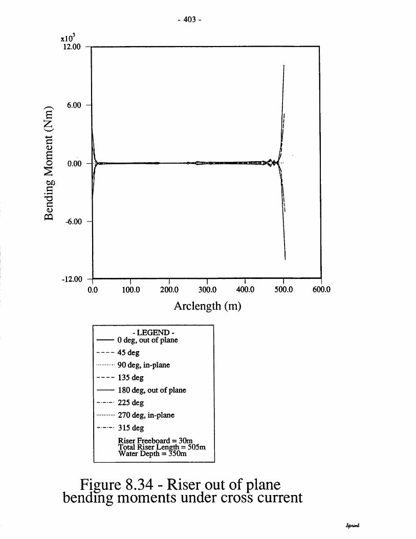
Bend

ing

Mom

ent

(Nm

)

- 403 -

xlO12.00

6.00 -

0.00 -

-6.00 -

■12.00100.0 200.0 300.0 400.0

Arclength (m)

500.0



600.0

Figure 8.34 - Riser out of planebending moments under cross current

Tors

ion

(Nm

)

- 404-

20.00

10.00

0.00

- 10.00

-20.00400.0 500.0100.0 300.0 600.00.0 200.0

Arclength (m)



Figure 8.35 - Riser torsions undercross current

Ver

tical

Pro

ject

ion

(m)

- 405 -

400.0

300.0 -

200.0 -

1 0 0 . 0 -

150.0 250.0-50.0 50.0


- LEGEND - Superposition (static

current) Combined (dynamic current)^ Uc = 0.5 m/s

O Uc = 0.1 m/s

FREQUENCY DOMAINUm = 2.618 m/s (surface)Wave Height = 10m Wave Period = 12s

Figure 8.36 - Comparison of displacement envelopes using static and

dynamic current models

- 4 0 6 -

U = 0.5 m/s40.00

30.00

020.00

10.00

0.00100.0 130.0 200.0 230.0 300.00.0

Arclength (m)

U = 0.1 m/s40.00

30.00

[20.00

10.00

0.00 30j0 200.0 230.0 300.00.0 100.0 130.0

Arclength (m)

- LEGEND- Stmpoakiao («Mfc cwraal)Ccnbnad (dynandc a n M ) FREQUENCY DOMAIN

U .« 24111 iqfi ( a ih n )

Figure 8.37 - Comparison of tensileforces with different current and wave

combinations

W

Ver

tical

Pro

ject

ion

(m)

- 407-

350.0

300.0 -

250.0 -

200.0 -

150.0100.0 150.050.0-50.0 0.0


- LEGEND - Wave Only Wave + Following Current Wave + Opposing Current

FREQUENCY DOMAIN

IL = 1 m/s= 2.618 m/s (surface)

Wave Height = 10m Wave Period = 12s

Figure 8.38 - Comparison ofdisplacement envelopes for different

current and wave combinations

- 408 -

«IO>40.00

.00

.00

0.00 IM.0 3000 300000Arclength (m)

»io'13.00

7.30

}J0.00

-7 JO

13.0030 0 IOOO

Arclength (m)

»io*

I

!■>jOO

rjo

050.0

Arclength (m)

♦ Oppastof CwnrmntBQUENCY DOMAIH

Figure 8.39 - Comparison of forces andmoments with different current and wavecombinations

dfnu

Ver

tical

Pro

ject

ion(

m)

- 40 9 -

400.0

320.0 -

240.0 -

160.0 -

80.0 -

0.0 -300.0220.060.0 140.0- 100.0 -20.0

Horizontal Projection(m)

-LEGEND -

Minimum (Frequency Domain) Maximum (Frequency Domain) Time Domain TrajectoriesWave Height = 20m Wave Period = 16s Surge Amplitude = 6m Surge Phase a -90 deg Heave Amplitude = 4m Heave Phase = 0 deg

Figure 8.40 - Comparison of frequencyand time domain solutions

- 41 0 -

Tensile Forces-9.0

(2-10.0Vra

-11.060.00 90.00 120.0030.00

• LEGEND - Tim* Domain (U anr)

Time (s)

................. Tfam Dotmin (Nop Hnwr)— Prtqwncy Deem in

Bending Moments300.0

230.0

£g 200.0So2001 “eVffl

100.0

30.030.00 60.00 90.00 120.00

Time (s)

- LEGEND - Time Domain (linear)

............... Time Domain (Non-linear)-----------Frequency Domain

Figure 8.41 - Response time histories at sagbend in 2um, 16s regular seas

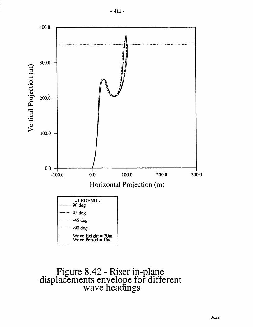
Ver

tical

Pro

ject

ion

(m)

- 411 -

400.0

300.0 -

200.0 -

100.0 -

0.0 -200.0 300.00.0 100.0-100.0


- LEGEND - 90 deg 45 deg

-45 deg -90 deg

Wave Height = 20m Wave Penod = 16s

Figure 8.42 - Riser in-planedisplacements envelope for different

wave headings

Ver

tical

Pro

ject

ion

(m)

- 412-

400.0

300.0

200.0

100.0

0.00.00 4.00 8.00-8.00 -4.00

Out of Plane Projection (m)

- LEGEND - 45 deg 0 deg -45 deg


Figure 8.43 - Side view of riserdisplacements envelope for different

wave headings

Out

of

Plan

e Pr

ojec

tion

(m)

- 413-

8.00

4.00 -

0.00

-4.00 -

-8.00 -120.030.0 90.00.0 60.0


- LEGEND - 45 deg Odeg -45 deg


Figure 8.44 - Plan view of riserdisplacements envelope for different

wave headings

Tens

ion

(N)

- 41 4 -

xlO330.00

18.00

6.00

-6.00

-18.00

-30.00440.0330.0 550.0110.0 220.00.0

Arclength (m)

- LEGEND - 90 deg 45 deg -45 deg

-90 deg+ Mean Static


!

Figure 8.45 - Riser tensile forceenvelope for different wave headings

Tors

ion

(Nm

)

- 415 -

0.450

0.220 - :v'

-0.010 -

-0.240 -

-0.470 -

-0.7000.0 100.0 200.0 300.0 400.0 500.0

Arclength (m)



Figure 8.46 - Riser torsion envelopefor different wave headings

Out

of

Plan

e Be

ndin

g M

omen

t (N

m)

- 416-

xlO31.500

0.900 -

0.300 -

-0.300 -

-0.900 -

-1.500 -400.0 500.0300.00.0 200.0100.0

Arclength (m)



Figure 8.47 - Riser out of planebending moment envelope for different

wave headings

Inpa

ne

Bend

ing

Mom

ent

(Nm

)

- 417 -

xlO31.500

0.900 -

0.300 -

vv>-0.300 -

-0.900 -

-1.500 — 0.0 100.0 200.0 300.0 400.0 500.0

Arclength (m)

- LEGEND - 90 deg 45 deg -45 deg -90 deg


Figure 8.48 - Riser in-plane bendingmoment envelope for different wave

headings

ipumt

- 418 -

SWL

E£*8H

105X1075jOO

Time (s)45X»30 JOO

140.0

50.0

IQSjOO900060003OJ0O

Time (s)

105.00

Tin* (■)

KJS.'E*

R gure 8.49 - Moment time histories atsWL for different wave headings

- 419-

SAGBEND7.60

4.60

-4.403000 45.00 6000 7500 9000

Time (s)

24.00

-36.003000 90007500 10300 12000

Time (s)

360.0

r >

J9

Time(s)

- LEGEND - ---------------- - 4 3 * ,..................... 04eg— ------43 * »-------------*>*g

wSRJsirrfi?

Figure 8.50 - Moment time histories atsagbend for different wave headings

- 420-

ARCH-TOP1.00

A4.10

-3.70

43.00 6000 7500 IOSjOO

Time (s)

I-*.00

sW*.00

3000 43.00 *001 1030)

Time (s)

/\

U>

10

Time (a)

- LBOBND----- ««•* «*»-----*o*(steias.-sr

Figure 8.51 - Moment time histories at arch top for different wave headings

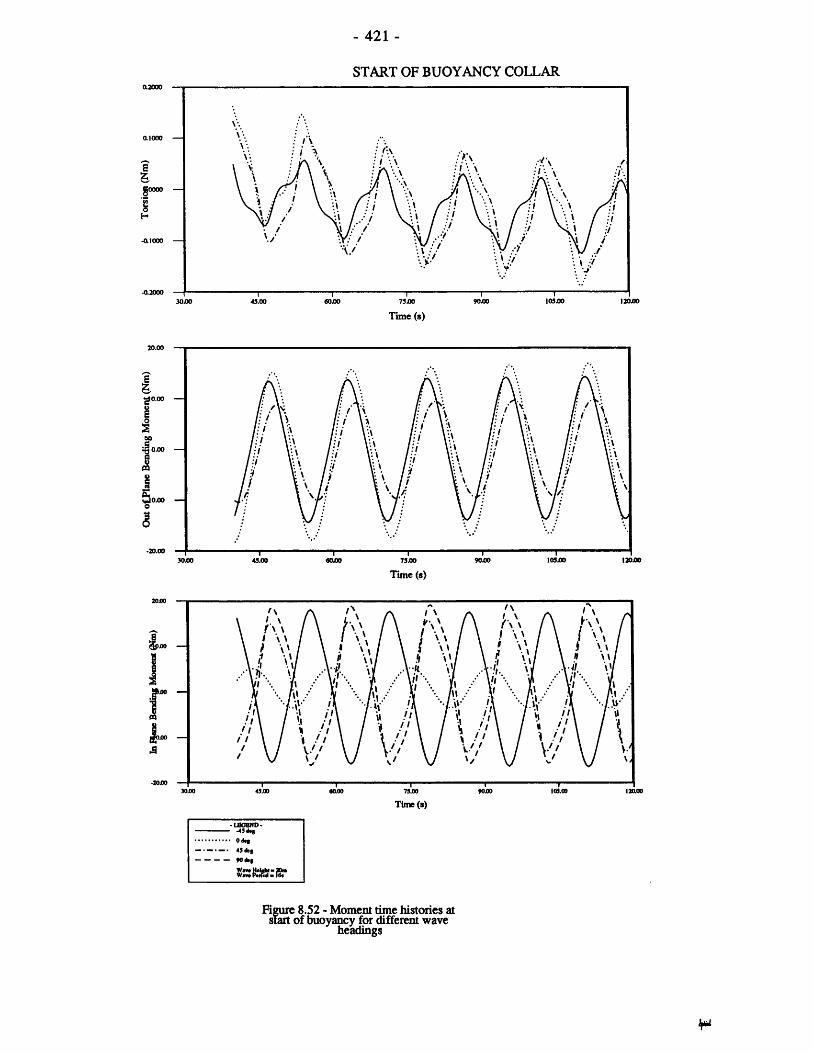
- 421 -

START OF BUOYANCY COLLAR

/ \

Soooo

IO5J0O73.0043.00 6000

Time (s)

20.00

0.00

S / A10.00

■20.00IOSjOO43.00

Time (s)

2000A \f\ \

)jOO

r\joo

«I>40

*040

-LSGBND- 11 ■ -43 * g....---— 43*g---- 90*8

Wo t Height-aOm Wo t t W a d - l*

Figure 8.52 - Moment time histories at start of buoyancy for different wave

headings

Snn

(m s/

rad)

- 422 -

150.0

100.0 -

50.0 -

0.25000 . 0 ----

0.0000 0.0833 0.1667

Frequency (Hz)

-LEGEND- ^ Discretised Spectrum Continuous Spectrum

Figure 8.53 - JONSWAP spectrum for 7msignificant, 10s sea state

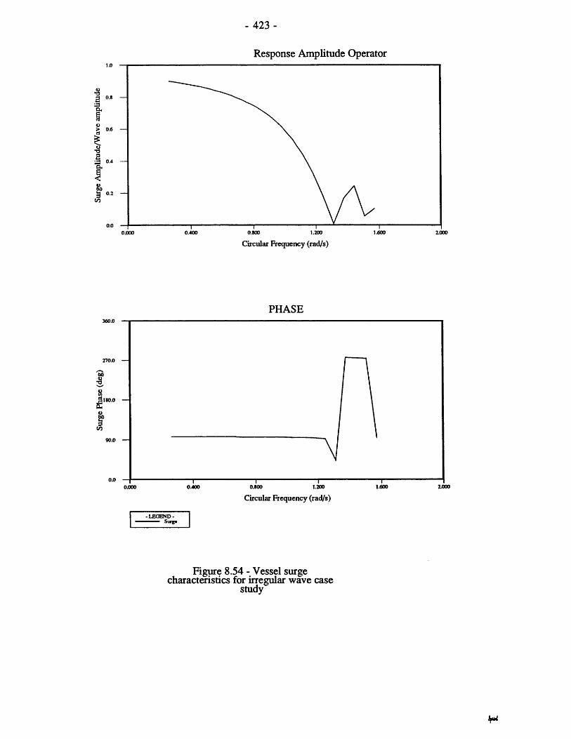
- 423 -

Response Amplitude Operator1.0

0.8

0.6

0.4

0.2

0.0 1.2000.400 0.800 2.0000.000

*82a,

I

Circular Frequency (rad/s)

PHASE360.0

270.0

1180.0

60

90.0

0.00.000 0.400 0.800 1.200 1.600 Z000


- LEGEND- Surge

Figure 8.54 - Vessel surgecharacteristics for irregular wave case

study

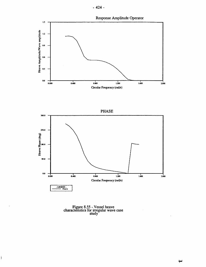
- 424-

Response Amplitude Operator1.5

13 0.6

0.3

0.01.6000.000 0.8000.400 1000


PHASE360.0

00

90.0 —

0.0 0.000 0.400 0.800 1.200 1.600 1000Circular Frequency (rad/s)

- LEGEND- ■■ H««v*

Figure 8.55 - Vessel heavecharacteristics for irregular wave case

study

i

Response Amplitude Operator

1.600 2.0001.2000.8000.4000.000Circular Frequency (rad/s)

PHASE

—f-----------1----------- 1----------- 1----------- 1-----------0.000 0.400 0.800 1.200 1.600 2.000


-LEGEND - Pitch

Figure 8.56 - Vessel pitchcharacteristics for irregular wave case

study

- 4 2 6 -

VESSEL MOTIONSj.

0.

-J.

Time (s)

SJ>

•J.0300.0OjO

Time (s)

OjM

OjOI

Itjoo

ffl

Time (a)

Figure 8.57 - Vessel surge, heave, pitch time histories in irregular seas

Spec

tral

Am

plitu

de

(m s/

rad)

- 427 -

12.00 -t

9.60 -

7.20 -

4.80 -

2.40 -

0.00 -0.0000 0.0833 0.1667 0.2500

Frequency (Hz)

- LEGEND - Surge Heave

Figure 8.58 - Simulated vessel surgeand neave spectra in 7m significant, 10s

sea state

hfifumL

- 428 -

SAGBEND

?x

300.0 400.0OjO

Time (s)

2.0

0.0

-2.03000IOOO

Time (s)

a)

ao 100.0 3O0LO«oaoTime (*)

l b o e n d -

Figure 8.59 - Displacement timehistories at sagbena in irregular seas

Spec

tral

Am

plitu

de

(m s/

rad)

- 42 9 -

3.500

2.800 -

2.100 -

1.400 -

0.700 -

0.000 -0.0900 0.27000.0000 0.1800

Frequency (Hz)

- LEGEND - X displacement Y displacement

Figure 8.60 - Simulated sagbend motionspectra in 7m significant, 10s sea state

Ver

tical

Pro

ject

ion

(m)

- 4 3 0 -

120.0

96.0 -

72.0 -

48.0 -

24.0 -

0.070.030.0 50.0-10.0 10.0-30.0-50.0


- LEGEND - Intermediate Profiles

Figure 8.61 - Lazy-wave response in 12m, 20s regular waves

- 431 -

xlO520.00

14.80 —

9.60 —

52 4.40

-0.80

-6.0040.0 80.0 120.0 160.0 200.00.0

Arclength (m)

-LEGEND-Static

— — — — Bounds (V ariable Seabed Contact)

................... Bounds (Fixed Seabed Contact)

Figure 8.62 - Bounds of tensile forces in 12m, 20s regular seas

xlO36.50

3.70

C 0.90

-1.90 —

-4.70

-7.5040.0 120.00.0 80.0 160.0 200.0

Arclength (m)

- LEGEND - ------------ Static----------- - Bounds (Variable Seabed

Contact)................ Bounds (Fixed Seabed Contact)

Figure 8.63 - Bounds of bending moments in 12m, 20s regular seas

Ver

tical

Pro

ject

ion

(m)

- 432 -

400.0

320.0 -

240.0 -

160.0 -Wave + Vessel + Slug

Wave + Vessel

80.0 -

0.0 -0.0 100.0 200.0 300.0 400.0- 100.0


-LEGEND- Riser Profile Slug: 230m, 25s Wave: 2.6m, 5s

Figure 8.64 - Combined wave, vessel andslug induced dynamics in 5 s regular sea

state

hptfwnl

- 433 -

400.0

320.0 -

sG.2 240.0 -■4— *o0)'o’J-iO h


t:<D>Wave + Vessel

80.0 -

0.0300.0 400.0- 100.0 0.0 100.0 200.0


-LEGEND- Riser Profile Slug: 230m, 25s Wave: 10.4m, 10s

Figure 8.65 - Combined wave, vessel andslug induced dynamics in 10s regular sea

state

Ver

tical

Pro

ject

ion

(m)

- 434-

400.0

320.0 -

240.0 -


Wave + Vessel

80.0 -

0.0300.0100.0 200.0- 100.0 0.0 400.0


-LEGEND- Riser Profile Slug: 230m, 25s Wave: 12m, 15s


state

- 435 -

400.0

320.0 -

ea.2 240.0 --4- ^o<L>'o'Ohcd 160.0 - o• ts<D>

Wave + Vessel + Slug

Wave + Vessel

80.0 -

0.0400.0300.0- 100.0 0.0 100.0 200.0


- L E G E N D - Riser Profile Slug: 230m, 25s Wave: 12m, 20s


state

Ver

tical

Pro

ject

ion

(m)

- 436-

400.0

320.0 -

240.0 -


Wave + Vessel

80.0 -

0.0- 100.0 100.0 200.0 300.0 400.00.0


-LEGEND- Riser Profile Slug: 230m, 25s Wave: 12m, 25s


state

Tens

ile

Forc

e (N

)

- 437 -

xlO3200.0

145.0 -

90.0

35.0 -

- 20.0

-75.0120.0 360.0240.0 480.0 600.00.0

Arclength (m)

- LEGEND - —I— Static Mean Wave + Vessel Wave + Vessel + Slug

Figure 8.69 - Typical tensile force envelope for wave, vessel and slug

induced dynamics in 25 s regular seastate

Bend

ing

Mom

ent

(Nm

)

- 438 -

xlO315.00

9.00 -

3.00 -

-3.00 -

-9.00 -

-15.00 -360.0120.0 240.0 480.0 600.00.0

Arclength (m)

- LEGEND - —I— Static Mean Wave + Vessel Wave + Vessel + Slug

Figure 8.70 - Typical bending moment envelope for wave, vessel and slug

induced dynamics in 25 s regular seastate

-439-

CHAPTER 9 : CONCLUSIONS

This work has presented a theoretical analysis and corresponding numerical analysis techniques for investigating the non-linear behaviour of a flexible riser subjected to forces induced by surface vessel motions, external wave and current forces and internal flow of contents. The results of the investigation are shown to have a considerable significance to the design of flexible risers for offshore applications. The main conclusions of the work are listed below grouped under the physical phenomena considered in each case.

PRESSURE FORCES

Three different derivations of pressure forces on pipes are presented. The first derivation provides the pressure forces for a segment of curved continuous pipe in two dimensions. This approach serves as a correction to the work of Young, et.al. (1978). The assumptions used are those of constant local curvature and small local angular change between the ends of the pipe element. This formulation is used to prove that the concept of effective tension, commonly utilised in two dimensional simulations, can be extended to three dimensions without loss of generality or accuracy.

The second derivation follows the approach suggested by Chakrabarti, et al. (1982) and showed their derivation to be in error. Corrected equations are given and shown to offer an exact result in two dimensions. The sole assumption of this derivation is that of constant local pipe curvature.

A novel third approach is developed to allow an exact integration of pressure forces over the surface of a flexible pipe in three dimensions. This formulation is constructed to enable the extension of flexible riser analysis into three dimensions where pipe curvature, whilst locally constant, falls into a non-vertical plane. The method is specially suited to computer applications and is easily programmable.

Static analysis of flexible pipes requires the modelling of these

-440-

pressure forces. This has been traditionally incorporated through the concept of effective tension. The methodology uses the grouping of the pressure and tension terms to advantage in calculation of the static profile of the pipe. It was found that the use of effective tension approach not only simplifies the calculations very significantly, but also avoids the numerical problems of modelling the pressure forces in the highly curved areas of the pipe. The use of this approach was proved to be valid for three dimensional analysis.

INTERNAL FLOW

A detailed examination of the static and dynamic influences of internal flow of fluids of constant and varying densities within a flexible pipe is conducted. This topic, which has not been addressed previously in the literature, is an emerging problem area and is one that has consistently been ignored in the past. The derivation of forces induced by a steady internal flow proves that:

"The effect of a steady internal flow on a continuously curved pipe is one of increasing the pipe wall tensions whilst leaving the effective tensions and hence pipe geometry unchanged. The mode of this interaction is analogous to the effect of internal pressures in the effective tension term. The magnitude of the changes in pipe wall tensions is independent of the flow direction and varies in proportion to the square of flow velocity."

The above statement is of utmost significance and whilst providing an elegant complement to the effective tension approach, suggests that dynamic changes in the density of the fluid flowing through the pipe will not only oscillate the geometry of the pipe, but also result in changes in its wall tensions. The validity of these stipulations are investigated through the development of a frequency domain and then a more detailed time domain analysis. The latter allowed the combined effects of wave, vessel and internal flow induced excitations to be studied simultaneously. Program results are compared with results from a series of model tests at University College London and show that significant geometric and tensile oscillations are generated by the flow of an internal fluid

-441-

of time variant density.

ANALYTICAL STATIC AND DYNAMIC ANALYSIS METHODS

A study of the use of analytical techniques in static and dynamic analysis of flexible pipe configurations was carried out. Multiple catenary solutions were found to offer very fast and accurate means of calculating the static profile of catenaries comprising of several sections of different weights and buoyancies. It was shown that most cases of practical interest may be analysed using these much simpler algorithms with no loss of accuracy whatsoever. Additionally, run times for the simpler methods were found to be of the order of seconds in contrast to 30-60 minutes typical of the equivalent numerical methods based on incremental shifting of the pipe to equilibrium.

Analytical solutions for dynamic analysis were found to be scarce and limiting in flexibility. Only selected geometries, such as the towed pipeline configuration, were found amenable to analysis using simple methods. A simplified dynamic analysis method was developed for towed pipelines and was shown to provide a useful preliminary design tool.

NUMERICAL STATIC ANALYSIS METHODS

Different methods for static analysis of flexible pipes were studied in two categories. The first examined the respective influence of tensile, geometric and loading non-linearities on the pipe forces and displacements. It was found that unless tensile and geometric non-linearities were considered in tandem, the pipetensions could be significantly underestimated. This effect was found to be very pronounced in the case of out of planedisplacements. A comparison with the results of O'Brien et al. (1988) showed that neglecting geometric non-linearity could lead to large overpredictions of the lateral displacements of the riser.

In cases involving a steady current on a static equilibrium riser geometry, non-linearities arising from deformation dependency ofloading on the pipe were found to be very small. This effect is,

-442-

nevertheless, of great significance with the incremental shifting procedures where the pipe geometry undergoes very large translations and rotations in space. In such cases a loading correction was found necessary at each shifting step but inter-step iterations were not required.

Development and use of the incremental shifting procedures proved these to be extremely difficult to implement and expensive to run. Implementation difficulties originated from the large rigid body displacements and rotations of the pipe and the resulting difficulty in calculating the pipe tensile forces from the displaced shape of the pipe. It was conlcuded that most cases of interest, if not all, could be analysed as accurately and with greatly reduced effort with the mutiple catenary solution algorithms. The use of incremental shifting techniques is not recommended for most applications.

NUMERICAL DYNAMIC ANALYSIS IN THE FREQUENCY DOMAIN

A linearised frequency domain dynamic analysis method was developed on the basis of the linearisation proposed by Krolikowski and Gay(1980). A suitable translation of the method to the finite element formulation was developed which is detailed in Chapter 6. Predictions of the program were validated through extensive comparisons against model test data, analytical results and publications by other investigators and overall agreement noted. The method was found accurate, rapidly convergent and ideally suited for regular wave analysis. The frequency domain programs are capable of analysing all common flexible riser geometries and include provisions for subsea buoys and vessels at both ends of the pipe. The advantage of the frequency domain method was found to be in its small time and storage requirements whilst its shortcoming was in analysis of irregular sea states and of resonant response.

NUMERICAL DYNAMIC ANALYSIS IN THE TIME DOMAIN

A non-linear time domain program was implemented for analysis of arbitrary flexible riser profiles in regular and irregular sea states. Comparisons with the frequency domain approach showed good

-443-

agreement. The method was used to examine the effects of wave heading, vessel motions, internal flow and non-linearities on the riser response. It was discovered that out of plane dynamic loads can be in excess of the in plane values. It was concluded that ignoring out of plane response can lead to non-conservative values in design.

SUGGESTIONS FOR FURTHER WORK

These studies have addressed several new aspects of flexible riser performance and attempted to improve upon the current understanding of flexible riser performance. The foremost area of concern was noted to be that involving the influence of internal flow on the dynamic response of flexible risers. It is demonstrated that the loading due to extreme slugs can be of comparable magnitude to those resulting from severe sea states. These effects place strong doubts on the suitability of the lazy-wave profile which is shown to be particularly susceptible to changes in its effective weight. It is felt necessary to continue work to establish,

a) a correlation between slug loadings and riser geometries to identify possibilities for optimisation of riser profiles,

b) implications of internal flows for operational, fatigue and wear limit state design of flexible riser,

c) recommendations for suitable response reduction techniques, be it in the form of modifications to the geometry or provision of purpose designed slug catchers,

d) a detailed understanding of non-linear interactions between external and internal loadings on the pipe.

-444-

REFERENCES

- Ansari K A, Khan N U; "The Effect of Cable Dynamics on Station Keeping Response of a Moored Offshore Vessel"; OMAE 1986, Tokyo, Japan

- American Petroleum Institute, API; "Comparison of Marine Drilling Riser Analysis"; API, Washington D. C., 1977

- Bathe K; "Finite Element Procedures in Engineering Analysis"; Prentice Hall, 1982

- Bernitsas M M, Hoff C J, Kokarakis J E; "Non-linear Inverse Purturbation in Structural Dynamics Redesign of Risers"; OMAE 1985, Houston, Texas

- Bernitsas M M, Kokarakis J E, Imron A; "Large Deformation Three-Dimensional Static Analysis of Deep Water Marine Risers"; Applied Ocean Research, 1985, Vol. 7, No. 4

- Bernitsas M M, Kokkinis T;"Global Static Instability of Risers"; Journal of Ship Research, Vol. 28, No. 4, Dec. 1984, pp. 261-271

- Bliek A, Koterayama W, Triantafyllou M S; "Dynamics of a Mooring Line Excited by an Ocean Structure in a Current"; OMAE 1986, Tokyo, Japan

- Borgman L E; "Ocean Wave Simulation for Engineering Design"; Proceedings of the ASCE, Journal of Waterways and Harbors Division, November 1969

- Bratu Ch., Narzul P; "Dynamic Behaviour of Flexible Riser"; BOOS, 1985, Amsterdam, Netherlands

- Brebbia C A, Walker S; "Dynamic Analysis of Offshore Structures"; Newnes-Butterworths, 1979

-445-

- Chakrabarti S K, Frampton R E; "Review of Riser Analysis Techniques"; Applied Ocean Research, 1982, Vol. 4, No. 2

- Clough R W, Penzien J; "Dynamics of Structures"; McGraw Hill, 1982

- Cowan R, Andris R P; "Total Pipelaying System Dynamics"; OTC 2914, 1977, Houston, Texas

- Eatock Taylor R, Rajagopalan A; "Load Spectra for Slender Offshore Structures in Waves and Currents"; Earthquake Engineering and Structural Dynamics; Vol. 11, 1983

- Engseth A, Bech A, Larsen C M; "Efficient Method for Analysis of Flexible Risers"; BOOS 88, Trondheim, Norway, 1988

- Fee D A, O'Dea J; "Technology for Developing Marginal Offshore Fields"; Elsevier Applied Science Publishers, London/New York, 1986

- Felippa C A, Park K C; "Computational Aspects of TimeIntegration Procedures in Structural Dynamics, Part 1:Implementation"; Journal of Applied Mechanics; September 1978, Vol. 45

- Felippa C A, Park K C; "Computational Aspects of TimeIntegration Procedures in Structural Dynamics, Part 2: Error Propagation"; Journal of Applied Mechanics; September 1978, Vol. 45

- Gardner T N, Kotch M A; " Dynamic Analysis of Riser and Caissons by the Element Method"; OTC(2651), 1976; Houston, Texas

- Gelb A, Vander Velde W E; "Multiple-input describing Functions and Non-linear System Design"; New York; McGraw-Hill; 1968

-446 -

- Ghadimi R, Kirk C L, Langley R S; "SERC Research Programme on the Dynamics of Compliant Structures, Project 11, Dynamic Analysis of Flexible Catenary Risers, Final Report"; June 1987, UK

- Gumestad 0 T, Connor J J; "Linearisation Methods and the Influence of Current on the Non-linear Hydrodynamic Drag"; Applied Ocean Research, 1983, Vol. 5, No. 4

- Hamilton J; "Three-dimensional Fourier Analysis of Drag Force for Compliant Offshore Structures"; Applied Ocean Research, 1980, Vol. 2, No. 4

- Hansen H T, Bergan P G; "Non-linear Dynamic Analysis of Flexible Risers During Environmental Loading"; OMAE 1986, Tokyo, Japan

- Hashemi Safai V H; "Non-Linear Dynamic Analysis of Deep Water Risers"; Applied Ocean Research, 1983, Vol. 5, No. 4

- Hasselmann K; "Measurement of Wind Wave Growth and Swell Decay During the Joint North Sea Wave Project"; Deut. Hydrogr. Z . , Reihe A, No. 12, 1973

- Huang T, Chucheepsakul S; "Large Displacement Analysis of a Marine Riser"; OMAE 1985, Houston, Texas

- Huang T, Rivero C E; "On the Functional in a Marine Riser Analysis"; OMAE 1986, Tokyo, Japan

- Isherwood R M; "Technical Note: A Revised Parameterisation of the JONSWAP Spectrum"; Applied Ocean Research, Vol. 9, No. 1, 1987

- Kao S; "An Assessment of Linear Spectral Analysis Methods for Offshore Structures via Random Sea Simulation"; Journal of Energy Resources Technology; Transactions of the ASME; March 1982, Vol. 104

-447-

- Kato N, Koda S, Takahashi T; "Motions of Underwater Towed Systems"; OMAE 1985, Houston, Texas

- Kim Y C; "Natural Frequencies and Critical Buckling Loadsof Marine Risers"; OMAE 1986, Tokyo, Japan

- Kim Y C, Triantafyllou M S; "The Non-Linear Dynamics ofSlender Cylinders"; OMAE 1985, Houston, Texas

- Kirk C L; "Dynamic Response of Marine Risers by Single Wave and Spectral Analysis Methods"; Applied Ocean Research, Vol. 7, No. 1, 1985

- Kirk C L, Etok E U; "Wave Induced Random Oscillations ofPipelines During Laying"; Applied Ocean Research, 1979, Vol. 1, No. 1

- Kirk C L, Etok E U, Cooper M T; "Dynamic and Static Analysis of a Marine Riser"; Applied Ocean Research, Vol. 1, No. 3, 1979

- Kitazawa I; "Three-Dimensional Analysis for Submarine Cables"; OMAE 1986, Tokyo, Japan

- Kreyszig E; "Advanced Engineering Mathematics"; 4th e d . , John Wiley, 1979

- Krolikowski L P; "An Improved Linearization Technique for Frequency Domain Riser Analysis"; OTC 3777, 1980, Houston, Texas

- Langer C G; "Relationships for Deep Water Suspended Pipe Spans"; OMAE 1985, Houston, Texas

- Langley R S; "The Linearisation of Three Dimensional Drag Force in Random Seas with Current"; Applied Ocean Research; 1984, Vol. 6, No. 3

-448-

- Larsen C M, Bech A; "Stress Analysis of Marine Risers under Lock-In Condition"; OMAE 1986, Tokyo, Japan

- Leira B J, Remseth S N; "A Comparison of Linear and Non-linear Methods for Dynamic Analysis of MarineRisers"; BOOS 1985

- Leira B J ; "Multidimensional Stochastic Linearisation of Drag Forces"; Applied Ocean Research; 1987, Vol. 9, No. 3

- Malahy R C; "A Non-linear Finite Element Method for the Analysis of Offshore Pipelines, Risers and Cable Structures"; OMAE 1986, Tokyo, japan

- Mathisen K M, Bergan P G;"Nonlinear Static Analysis of Flexible Risers"; OMAE 1986, Tokyo, Japan

- Mclver D B; "The Linear Stiffness of Mooring Catenaries"; Presented at a short course on "Dynamics ofCompliant Structures, Centre for Advanced Engineering- Studies", Southampton, 20-22 March 1985

- Mclver D B, Lunn T S; "Improvements to Frequency-Domain Riser Programs"; OTC 4559, 1983, Houston, Texas

- Mclver D B, Olson R J; "Riser Effective Tension - Now You See It, Now You Don't!", Risers, Arctic Design Criteria, Equipment, Reliability in Hydrocarbon Processing; 37th. Petroleum Mechanical Engineering Workshop & Conference; dallas, Texas, September 1981

- McNamara J F, O'Brien P J, Gilroy S G; "Non-linearAnalysis of Flexible Risers Using Hybrid Finite Elements"; OMAE 1986, Tokyo, Japan

- Meriam J L; "Engineering Mechanics, Statics"; Vol 1,Wiley, New York, 1980

-449-

- Narzul P, Marion A; "Static and Dynamic Behaviour of Flexible Catenary Risers"; OMAE 1986, Tokyo, Japan

- Natvig B J; "A Large Angle - Large Displacement Analysis Method for Marine Risers"; Presented at Intermaritec 80, September 1980, Hamburg, West Germany

- Nordgren, R P; "On Computation of the Motion of Elastic Rods"; Journal of Applied Mechnaics; Transactions of the ASME; September 1974

- Nordgren, R P; "Dynamic Analysis of Marine Risers with Vortex Excitation"; Journal of Energy Resources Technology; Transactions of the ASME; Vol. 104, March 1982

- O'Brien P J, McNamara J F, Dunne F P E ; "Three-Dimensional Non-linear Motions of Risers and Offshore Loading Towers"; OMAE 1987, Houston, Texas

- O'Brien P J, McNamara J F; "Analysis of Flexible Riser Systems Subject to Three Dimensional Sea State Loading"; BOOS 88, Trondheim, Norway 1988

- Ochi, M K; "Stochastic Analysis and Probabilistic Prediction of Random Seas"; Advances in Hydroscience; Academic Press; Vol. 13; 1982

- Odru P, Guichard J C; "Drilling Risers for Great Water Depths: Advantage of Mass Reduction by Means of Composite Materials", Third Deep Offshore Technology Conference and Exhibition, 1985, Italy

- Orgill G, Wilson J F, Schmertmann G R; "Static Design of Mooring Arrays for Offshore Guyed Towers"; Applied Ocean Research, 1985, Vol. 7, No. 3

- Owen D G, Qin K; "Model Tests and Analysis of Flexible Riser Systems"; OMAE 1986, Tokyo, Japan

-450-

- Owen D G, Qin J J; "Non-linear Dynamics of Flexible Risers by the Finite Element Method"; OMAE 1987, Houston, Texas

- Patel M H, Sarohia S, "Dynamic response of Free hanging Risers in Waves ", Proceedings of the Third Offshore Mechanics, Arctic Engineering and deep Sea Symposium, 1983

- Patel M H, Sarohia S , Ng K F; "Finite Element Analysis of the Marine Riser"; Engineering Structures, 1984, Vol. 6

- Patel M H; Final Report; "Dynamics of Compliant Structures"; A Managed Programme of Research, 1985-87; London Centre for Marine Technology; University College London; London, England; October 1987

- Peyrot A H, Goulois A M; "Analysis of Cable Structures"; Computers & Structures, Vol. 10, pp 805-813, 1978

- Polderdijk S H; "Response of Anchor Lines to Excitation at the Top"; Behaviour of Offshore Structures, 1985, Amsterdam, Netherlands

- Pierson W J, Moscowitz L; "A Proposed Spectral Form for Fully Developed Wind Seas based on the Similarity Theory of S.A. Kitaigorodskii"; Journal of Geophysics Research; Vol. 69, pp. 5181-5190, 1964

- Ractliffe A T; "The Validity of Quasi-Static and Approximate Formulae in the Context of Cable and Flexible Riser Dynamics"; BOOS 1985, Amsterdam,Netherlands

- Redshaw P R, Stalker A W; "Explosive Welding Combines with Bottom Tow for New Subsea Pipeline Construction Technique"; OTC(3523), 1976; Houston, Texas

- Rodenbusch G, Garrett D L, Anderson S L; "Statistical Linearisation of Velocity-Squared drag Force"; BOOS, 1985

-451-

- Rooduyn E J, Boonstra H; "Design Aspects of the Controlled Bottom Tow Method for Pipeline Bundles"; The 3rd Deep Offshore Technology Conference; Vol I; 1985; Italy

- Sarpkaya T, Isaacson M; "Mechanics of Wave Forces on Offshore Structures"; Van Nostrand Reinhold; 1981

- Sparks C P; "Mechanical Behaviour of Marine Risers Mode of Influence of Principal Parameters"; Proceedings of the Winter Annual Meeting of the American Society of Mechanical Engineers"; 2-7 December 1979, OED Vol. 7, New York

- Sparks C P, Cabillic J P, Schawann J C; "Logitudinal Resonant Behaviour of Very Deep Water Risers"; OTC 4317, 1982, Houston, Texas

- Sparks C P; "The Influence of Tension, Pressure and Weight on Pipe and Riser deformations and Stresses"; Journal of Energy Resources Technology; Transactions of ASME; Vol 106, March1984

- Thomson W T; "Theory of Vibration with Applications"; Allen & Unwin; London, 1981

- Timoshenko S P, Young D H; "Theory of Structures"; Me Graw Hill; 2nd edition; 1965

- Tonda H, Dorel M; "Experimental Study of Upwards Gas-Drilling Fluids Flows"; Third Deep Offshore Technology Conference and Exhibition, 1985, Italy

- Tucker M J, Challenor P G, Carter D J T; "Numerical Simulation of Random Sea: A Common Error and its Effects upon Wave group Statistics"; Applied Ocean Research; 1984 Vol. 6, No. 2

- Van den Boom H J J; "Dynamic Behaviour of Mooring Lines"; BOOS1985

-452-

- Vogel H, Natvig B J; "Dynamics of Flexible Hose Riser Systems"; OMAE 1986, Tokyo, Japan

- Warburton G B; "The Dynamical Behaviour of Structures"; McGraw-Hill, 1982

- Weaver W Jr, Gere J M; "Matrix Structural Analysis"; 2nd. ed; D. Van Nostrand Company, 1980

- Wu S C, McDermott J R; "The Effects of Current on Dynamic Response of Offshore Structures"; OTC 2540; Dallas, Texas; 1976

- Young R D, Fowler J R; "Mathematics of Marine Risers"; The Energy Technology Conference and Exhibition, November 1978, Houston, Texas

- Young R D, Fowler J R, Fisher E A, Luke; "Dynamic Analysisa as an Aid to the Design of Marine Risers"; Transactions of the ASME, Vol. 100, May 1978

- Zienkiewicz 0 C; "The Finite Element Method"; 3rd. ed; McGraw Hill, 1983

on the dynamics of flexible risers and suspended …

Documents