on the capacity of distributed antenna systemslindai/das.pdf · on the capacity of distributed...
TRANSCRIPT

Jun. 25, 2014
1
On the Capacity of Distributed Antenna Systems
Lin Dai
City University of Hong Kong

Jun. 25, 2014
2
Cellular Networks (1)
Multiple antennas at the BS side
Base Station (BS)
Growing demand for high data rate
Jun. 25, 2014
3
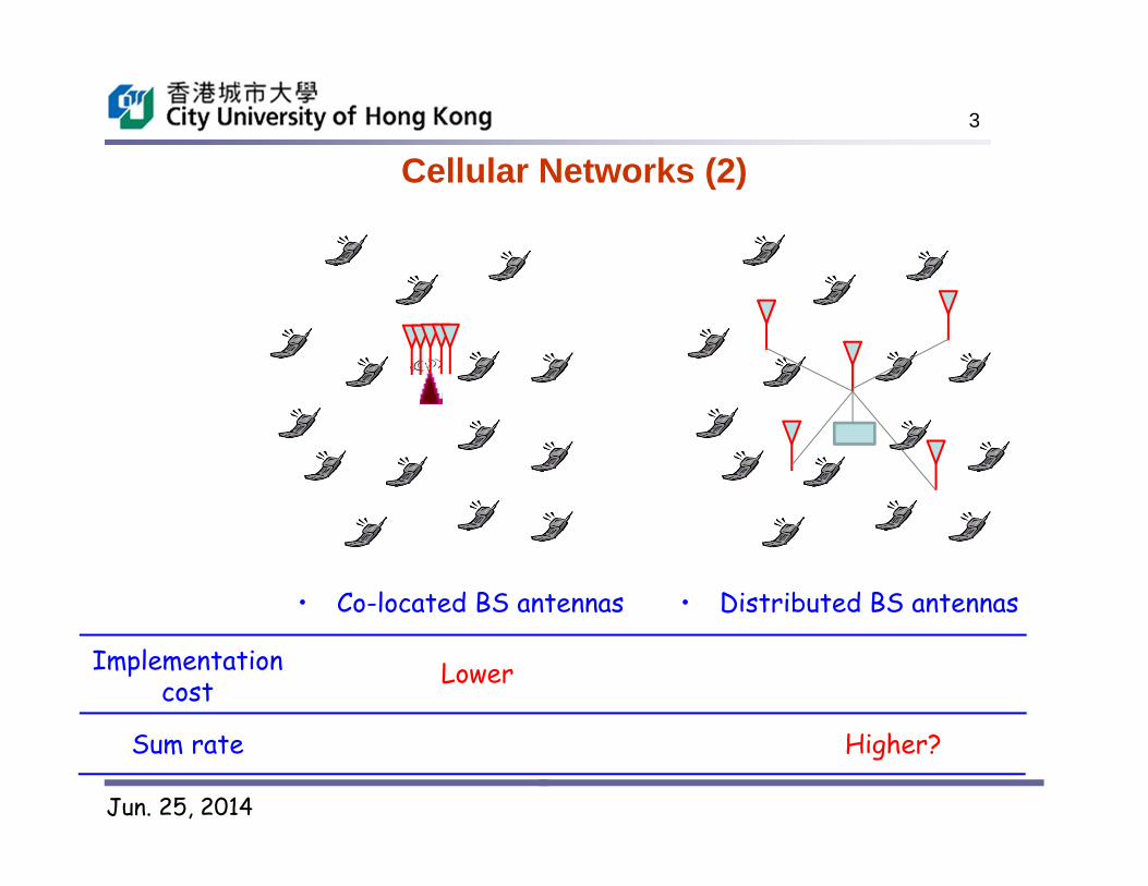
Cellular Networks (2)
• Co-located BS antennas • Distributed BS antennas
Implementation cost
Sum rate
Lower
Higher?
Jun. 25, 2014
A little bit of History of Distributed Antenna Systems (DASs)
• Originally proposed to cover the dead spots for indoor
wireless communication systems [Saleh&etc’1987].
• Implemented in cellular systems to improve cell coverage.
• Recently included into the 4G LTE standard.
• Key technology for C-RAN and 5G?
• Multiple-input-multiple-output (MIMO) theory has motivated
a series of information-theoretic studies on DASs.
4

Jun. 25, 2014
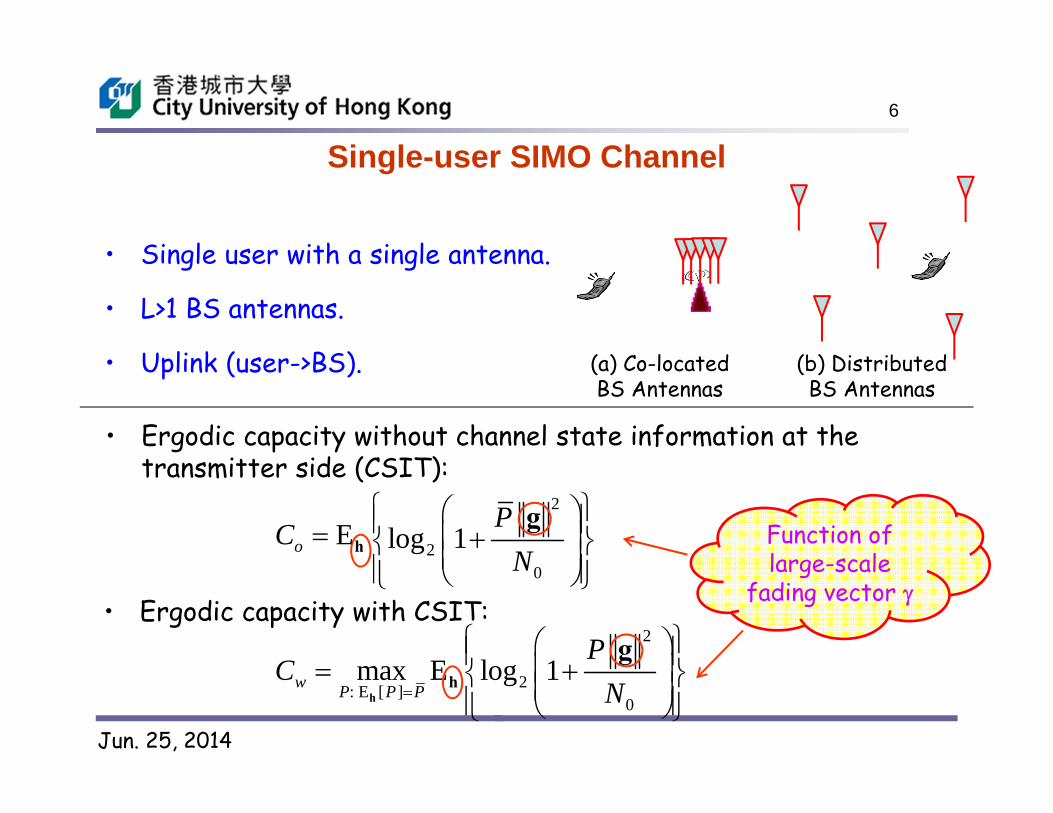
Single-user SIMO Channel
• Single user with a single antenna.
• L>1 BS antennas.
• Uplink (user->BS). (a) Co-located BS Antennas
(b) Distributed BS Antennas
5
s y g z• Received signal:
g = γ h• Channel gain : : Large-scale fading
: Small-scale fading
1LC γ
1LC h
: Transmitted signal: Gaussian noise
(0, )s P 1LC z
0(0, ), 1,..., .iz N i L
(0,1), 1,..., .ih i L
/2 2Log ( , ), 1,..., .i i id i L
Jun. 25, 2014
Single-user SIMO Channel
2
20
log 1P
N
g
• Ergodic capacity without channel state information at the transmitter side (CSIT):
• Single user with a single antenna.
• L>1 BS antennas.
• Uplink (user->BS).
• Ergodic capacity with CSIT:2
2: E [ ]0
max E log 1w P P P
PC
N
hh
g
Function of large-scale
fading vector
(a) Co-located BS Antennas
(b) Distributed BS Antennas
6
EoC h
Jun. 25, 2014
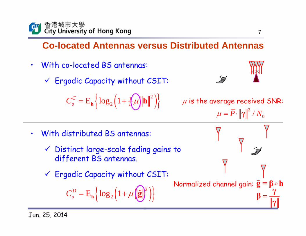
Co-located Antennas versus Distributed Antennas
• With co-located BS antennas:
Ergodic Capacity without CSIT:
212E log 1C
o LC h h is the average received SNR:2
0/P N γ
• With distributed BS antennas:
Distinct large-scale fading gains to different BS antennas.
Ergodic Capacity without CSIT:
22E log 1D
oC h gNormalized channel gain:
7
g = β h
γβγ

Jun. 25, 2014
Capacity of DAS8
• For given large-scale fading vector : [Heliot&etc’11]: Ergodic capacity without CSIT
o A single user equipped with N co-located antennas.o BS antennas are grouped into L clusters. Each
cluster has M co-located antennas.o Asymptotic result as M and N go to infinity and
M/N is fixed. [Aktas&etc’06]: Uplink ergodic sum capacity
without CSITo K users, each equipped with Nk co-located
antennas. o BS antennas are grouped into L clusters.
Each cluster has Nl co-located antennas.o Asymptotic result as N goes to infinity and
k and l are fixed.
• Implicit function of (need to solve fixed-point equations)
• Computational complexity increases with L and K.

Jun. 25, 2014
Capacity of DAS
[Choi&Andrews’07], [Wang&etc’08], [Feng&etc’09], [Zhu’11], [Lee&ect’12]: BS antennas are regularly placed in a circular cell and the user has a random location.
9
Average ergodic capacity (i.e., averaged over )
[Zhuang&Dai’03]: BS antennas are uniformly distributed over a circular area and the user is located at the center.
[Roh&Paulraj’02], [Zhang&Dai’04]: The user has identical access distances to all the BS antennas. 2Log (1, ), 1,..., .i i L
/2 , 1,..., .i i i L
/2 2Log ( , ), 1,..., .i i id i L
Computational complexity increases with the number of BS antennas!
• With random large-scale fading vector :
Single user Without CSIT
Jun. 25, 2014
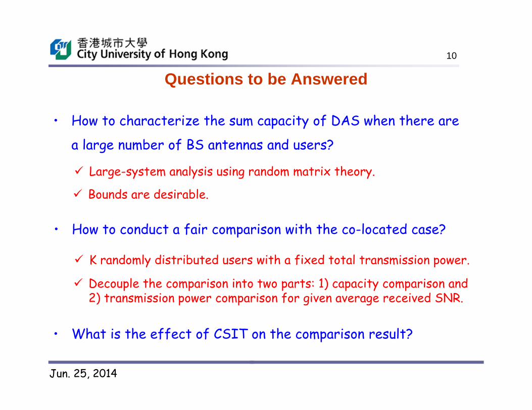
Questions to be Answered
• How to characterize the sum capacity of DAS when there are
a large number of BS antennas and users?
• How to conduct a fair comparison with the co-located case?
Large-system analysis using random matrix theory.
• What is the effect of CSIT on the comparison result?
Decouple the comparison into two parts: 1) capacity comparison and 2) transmission power comparison for given average received SNR.
K randomly distributed users with a fixed total transmission power.
10
Bounds are desirable.

Jun. 25, 2014
Outline
• Single-cell comparison
• Multi-cell comparison
• DAS with virtual cells
11
[1] L. Dai, “A Comparative Study on Uplink Sum Capacity with Co-located
and Distributed Antennas,” IEEE J. Sel. Areas Commun., 2011.
[2] L. Dai, “An Uplink Capacity Analysis of the Distributed Antenna
System (DAS): From Cellular DAS to DAS with Virtual Cells,” IEEE
Trans. Wireless Commun., 2014.

Jun. 25, 2014
12
Part I. Single-Cell Comparison
• System model and preliminary analysis
• Uplink ergodic sum capacity
• Average transmission power per user

Jun. 25, 2014
13
System Model and Preliminary Analysis

Jun. 25, 2014
Assumptions
• K single-antenna users are uniformly distributed within a circular cell.
• L BS antennas are either co-located at the center of the cell, or uniformly distributed over the cell.
• Uplink (user->BS).
(a) Co-located Antennas (CA) (b) Distributed Antennas (DA)
*: usero: BS antenna
14
Random BS antenna layout!

Jun. 25, 2014
Uplink Ergodic Sum Capacity
k k kg = γ h1
K
k kk
s
y g z
• Received signal: : Transmitted signal: Gaussian noise
(0, )k ks P 1LC z
: Large-scale fading
: Small-scale fading
1Lk C γ
1Lk C h
0(0, ), 1,..., .iz N i L
: Channel gain
• Uplink power control:2
0 , 1,..., .k kP P k K γ
†_ 2
10
†02
10
1=E log det
=E log det
K
sum o L k k kk
K
L k kk
C PN
PN
H
H
I g g
I g g
Ergodic capacity without CSIT
0
†_ 2: E [ ] 101,...,
†2: E [ ] 101,...,
1= max E log det
1= max E log det
k k k
k k
K
sum w L k k kP P P kk K
K
L k k kP P P kk K
C PN
PN
H
H
H
H
I g g
I g g
Ergodic capacity with CSIT
15
, (0,1), 1,..., .i kh i L
/2, , , 1,..., .i k i kd i L

Jun. 25, 2014
More about Normalized Channel Gain
• Normalized channel gain vector:
k k kg = β h : Normalized
Large-scale fading
: Small-scale fading1Lk
kk
C γβγ
1Lk C h
With CA:
, , , .i k j k i j With DA:
11 .k LL β 1
o With a large L, it is very likely that user k is
close to some BS antenna :*kl *
kk lβ e
*1 if 0 otherwise
kl
l le
if .L 2 1k g
*
2 2,
| |k
k l khg
The channel becomes deterministic with a large number of BS
antennas L!
Channel fluctuations are preserved even
with a large L!
16
1.k β
Jun. 25, 2014
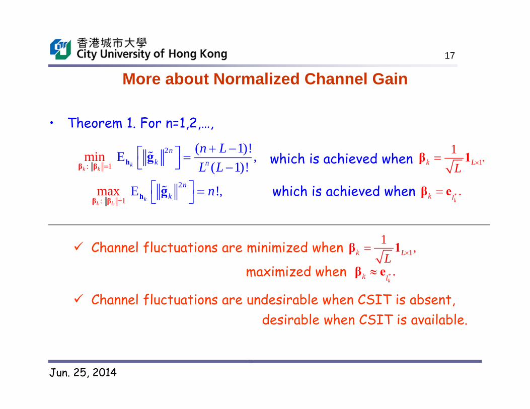
More about Normalized Channel Gain
• Theorem 1. For n=1,2,…,
: 1
2min ( 1)!E ,( 1)!k
kk
nk n
n LL L
β β h g
:
2
1max E !,
kk k
nk n
β hβg
which is achieved when
which is achieved when
11 .k LL β 1
* .k
k lβ e
Channel fluctuations are minimized when
maximized when * .k
k lβ e
11 ,k LL β 1
Channel fluctuations are undesirable when CSIT is absent,desirable when CSIT is available.
17

Jun. 25, 2014
Single-user Capacity (1)2
0lo
g(1
)k
C
_Ck oC _
Ck wC
*_
Dk oC
*_
Dk wC
*k
k lβ e
(average received SNR) 0 0 0/ (dB)P N
• Without CSIT -- Fading
always hurts if CSIT is absent!
_ / 1k o AWGNC C
quickly approaches 1 as L grows.
_ /Ck o AWGNC C
*
_ _C Dk o k oC C
• With CSIT (when 0 is small)
_ / 1k w AWGNC C
*_ _
D Ck w k wC C
at low 0
--“Exploit” fading
18

Jun. 25, 2014
Single-user Capacity (2)
The average received SNR . 0 0dB
• Without CSIT
• With CSIT
A higher capacity is achieved in the CA case thanks to better diversity gains.
A higher capacity is achieved in the DA case thanks to better waterfilling gains.
AWGN 2 0log (1 )C
19
*k
k lβ eDA with
*k
k lβ eDA with

Jun. 25, 2014
20
Uplink Ergodic Sum Capacity
Jun. 25, 2014
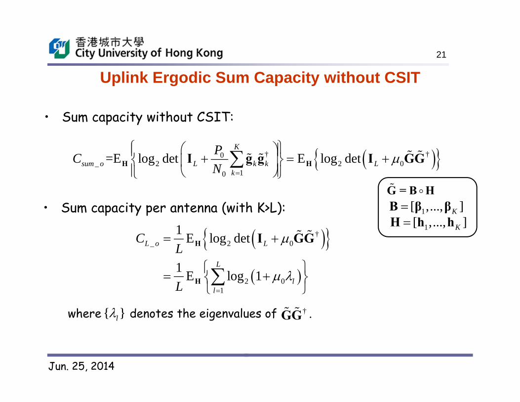
Uplink Ergodic Sum Capacity without CSIT
• Sum capacity without CSIT:
• Sum capacity per antenna (with K>L):
† †0_ 2 2 0
10
=E log det E log detK
sum o L k k Lk
PCN
H HI g g I GG
†_ 2 0
2 01
1 E log det
1 E log 1
L o L
L
ll
CL
L
H
H
I GG
G = B H 1[ ,..., ]KB β β1[ ,..., ]KH h h
where denotes the eigenvalues of . †GG { }l
21

Jun. 25, 2014
More about Normalized Channel Gain
• Theorem 2. As and
E [ ] , H
when * *1
[ ,..., ].Kl l
B e e
,K L / ,K L
and 2 2E [ ] 2 , H 0 . with
0
when 1 .L KL B 1
With DA and * *1
[ ,..., ] :Kl l
B e e
* ( )
0
( )( )!( 1)!
kD x
k
xf x ek k
as and ,K L / .K L
With CA:
2 21( ) (( 1) )( ( 1) )2
Cf x x xx
1 .L KL B 1
as and ,K L / .K L [Marcenko&Pastur’1967]
22
Jun. 25, 2014
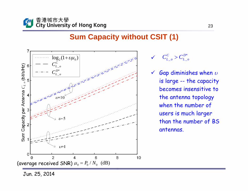
Sum Capacity without CSIT (1)
*
_ _C DL o L oC C
Gap diminishes when is large -- the capacity becomes insensitive to the antenna topology when the number of users is much larger than the number of BS antennas.
2 0log (1 )
_CL oC
*_
DL oC
(average received SNR) 0 0 0/ (dB)P N
23
Jun. 25, 2014
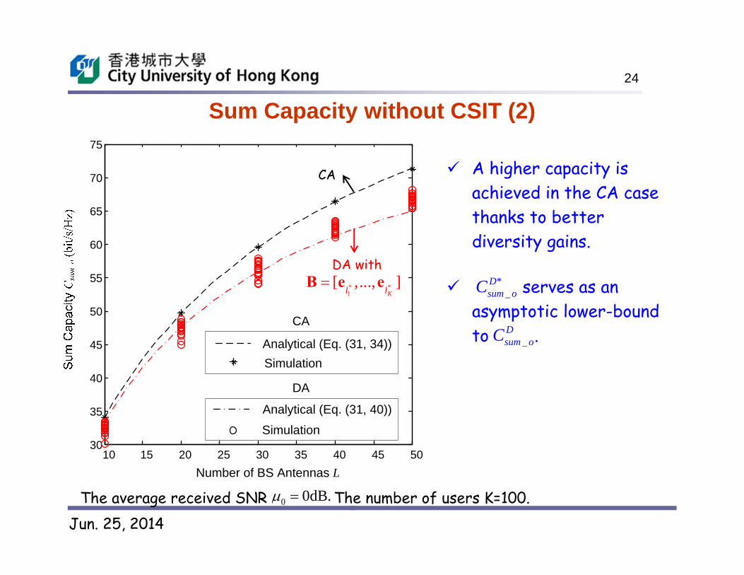
Sum Capacity without CSIT (2)
The average received SNR 0 0dB.
A higher capacity is achieved in the CA case thanks to better diversity gains.
10 15 20 25 30 35 40 45 5030
35
40
45
50
55
60
65
70
75
Number of BS Antennas L
CA
DA
Analytical (Eq. (31, 34))Simulation
Analytical (Eq. (31, 40))Simulation
The number of users K=100.
serves as an asymptotic lower-bound to .
*_
Dsum oC
_Dsum oC
24
* *1
[ ,..., ]Kl l
B e eDA with
CA

Jun. 25, 2014
Uplink Ergodic Sum Capacity with CSIT
• Sum capacity with CSIT:
0
†_ 2: E [ ] 101,...,
1= max E log detk k
K
sum w L k k kP P P kk K
C PN
H
H I g g
2
k k kP P γ
With CA:The optimal power allocation policy:
*
0 1† *
1 1k
k L j j j kj k
P NP
g I g g g
where is a constant chosen to meet the power constraint , k=1,…, K. [Yu&etc’2004]
0E kP PH
With DA andThe optimal power allocation policy:
*
* 2* 0 ,2
,
*
1 1 arg max | || |
0
ii
i i kkk i k
i
N k k hP h
k k
i=1,…,L, where is a constant chosen to meet the sum power constraint
01E .K
kkP KP
H
* *1
[ ,..., ] :Kl l
B e e
25
Jun. 25, 2014
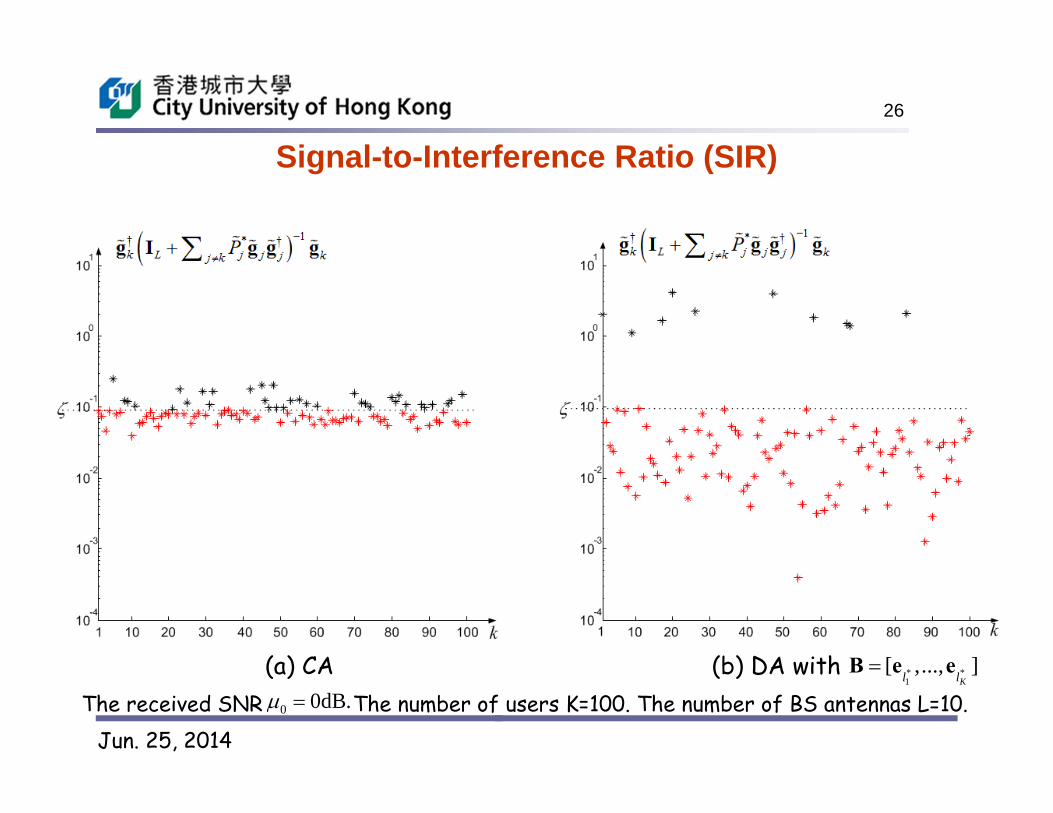
Signal-to-Interference Ratio (SIR)
(a) CA (b) DA withThe received SNR 0 0dB. The number of users K=100. The number of BS antennas L=10.
* *1
[ ,..., ]Kl l
B e e
26

Jun. 25, 2014
Sum Capacity (1)
20
log
(1)
sum
K L
CL
* *1
[ ,..., ]Kl l
B e e
* *1
[ ,..., ]Kl l
B e e
(average received SNR) 0 0 0/ (dB)P N
• Without CSIT
• With CSIT
Gap between and _Csum oC
*
_ _C Dsum o sum oC C
*_ _
D Csum o sum oC C
even at high SNR (i.e., thanks to better multiuser diversity gains)
*_
Dsum oC is enlarged as L grows
(i.e., due to a decreasing K/L).
27
The number of users K=100.

Jun. 25, 2014
Sum Capacity (2)
The average received SNR 0 0dB. The number of users K=100.
• Without CSIT
• With CSIT
A higher capacity is achieved in the CA case thanks to better diversity gains.
A higher capacity is achieved in the DA case thanks to better waterfilling gains and multiuser diversity gains.
28
* *1
[ ,..., ]Kl l
B e eDA with
CA

Jun. 25, 2014
29
Average Transmission Power per User

Jun. 25, 2014
Average Transmission Power per User
• Transmission power of user k: 02 , 1,..., .k
k
PP k K γ
With DA:
What is the distribution of2 ?kγ
• Average transmission power per user:
1
1 K
kk
PK
o Both users and BS antennas are uniformly distributed in the circular cell.
With CA:o Users are uniformly distributed
in the circular cell. BS antennas are co-located at cell center.
2k kL γ
2
2( )k
xf xR
022
C P RL
30
20
0( )
k
K P f x dxx
γ

Jun. 25, 2014
Minimum Access Distance
• With DA, each user has different access distances to different BS antennas. Let
denote the order statistics obtained by arranging the access distances d1,k,…, dL,k.
(1) (2) ( )Lk k kd d d
• for L>1.
• An upper-bound for average transmission power per user with DA:
2 (1),
1
L
k l k kl
d d
γ
(1)0
|0 0( ) ( | )
k kk
R R yD DUd
Pf y f x y dxdyx
2
2( )k
yf yR
(1) , ,
1| ||
( | ) (1 ( | )) ( | )l k k l k kkk
Ld dd
f x y L F x y f x y
2
2 2 2,2
2
| 22
0( | )
arccosl k k
xR
d x y RxxyR
x R yf x y
R y x R y
31

Jun. 25, 2014
Average Transmission Power per User
CA: 1C O L
2C
LL
A
vera
ge T
rans
mis
sion
Pow
er P
er U
ser
0 0D CP P
10 0 5D CP P L
1C L
DU
0 1CP
Path-loss factor =4.
DA: /2DU O L
(path-loss factor >2)
With =4, C D if1
0 0 5 .D CP P L
For given received SNR, a lower total transmission
power is required in the DA case thanks to the reduction of minimum access distance.
32

Jun. 25, 2014
Sum Capacity without CSIT
10 0 5 .D C L The number of users K=100.
• For fixed K and ( such that
0C
0C
33
_ 2 0log (1 / )C Csum oC L K L
_ ( )Dsum oC O L
0C
10 0 5D C L C D )
Given the total transmission power, a higher capacity is achieved in the DA case.
Gains increase as the number of BS antennas grows.
0 2logL
C K e

Jun. 25, 2014
Summary• A comparative study on the uplink ergodic sum capacity with co-
located and distributed BS antennas is presented by using large-system analysis. – A higher sum capacity is achieved in the DA case. Gains increase
with the number of BS antennas L.
– Gains come from 1) reduced minimum access distance of each user; and 2) enhanced channel fluctuations which enable better multiuser diversity gains and waterfilling gains when CSIT is available.
• Implications to cellular systems:– With cell cooperation: capacity gains achieved by a DAS over a
cellular system increase with the number of BS antennas per cell thanks to better power efficiency.
– Without cell cooperation: lower inter-cell interference with DA?
34

Jun. 25, 2014
35
Part II. Multi-Cell Comparison
• System model and preliminary analysis
• Uplink ergodic sum capacity
• Sum rate with orthogonal access

Jun. 25, 2014
36
System Model and Preliminary Analysis
Jun. 25, 2014
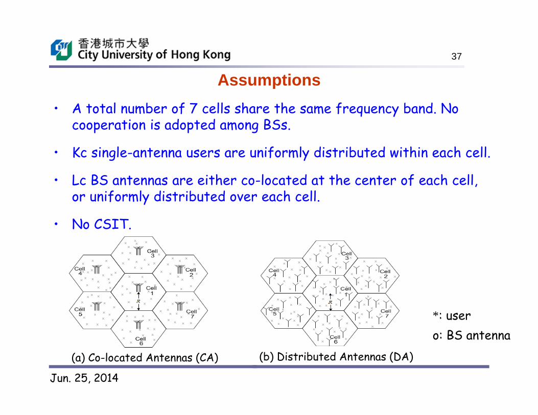
Assumptions• A total number of 7 cells share the same frequency band. No
cooperation is adopted among BSs.
• Kc single-antenna users are uniformly distributed within each cell.
• Lc BS antennas are either co-located at the center of each cell, or uniformly distributed over each cell.
• No CSIT.
(a) Co-located Antennas (CA) (b) Distributed Antennas (DA)
*: usero: BS antenna
37
Jun. 25, 2014
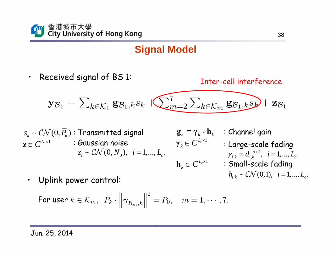
Signal Model
k k kg = γ h
• Received signal of BS 1:
: Transmitted signal: Gaussian noise
(0, )k ks P 1cLC z : Large-scale fading
: Small-scale fading
1cLk C γ
1cLk C h
0(0, ), 1,..., .i cz N i L
: Channel gain
• Uplink power control:
38
, (0,1), 1,..., .i k ch i L
/2, , , 1,..., .i k i k cd i L
Inter-cell interference
For user
Jun. 25, 2014
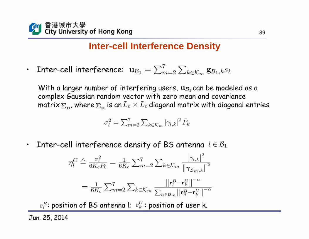
Inter-cell Interference Density
• Inter-cell interference:
39
With a larger number of interfering users, can be modeled as a complex Gaussian random vector with zero mean and covariance matrix , where is an diagonal matrix with diagonal entries
• Inter-cell interference density of BS antenna
: position of BS antenna l; : position of user k.

Jun. 25, 2014
Inter-cell Interference Density
• Theorem 1. The inter-cell interference density of BS antenna in cellular systems with the CA layout
40
• Theorem 2. The average inter-cell interference density of BS antenna in cellular systems with the DA layout is upper-bounded by
where
where

Jun. 25, 2014
Inter-cell Interference Density
CA: 1CCl cL
Path-loss factor =4.
DA:
(path-loss factor >2)
41
/2CDul cL
decreases at a higher rate than as the number of BS antennas per cell Lc increases.
CCl
CDl
With the DA layout, the inter-cell interference density significantly varies with the position of the BS antenna.
Jun. 25, 2014
42
Uplink Ergodic Sum Capacity

Jun. 25, 2014
Uplink Ergodic Sum Capacity
• Normalized sum capacity:
43
: eigenvalues of
: average received SINR of BS antenna
Asymptotic normalized sum capacity with CA:
An asymptotic lower-bound of the normalized sum capacity with DA:
• As and :
where where

Jun. 25, 2014
Uplink Ergodic Sum Capacity
• As P0/N0 increases:
• Substantial gains can be achieved in the DA case owing to the improvement in the inter-cell interference density.
DA: grows unboundedly.
CA: converges to a function of .
44
Path-loss factor
CCkC
CDlkC
Jun. 25, 2014
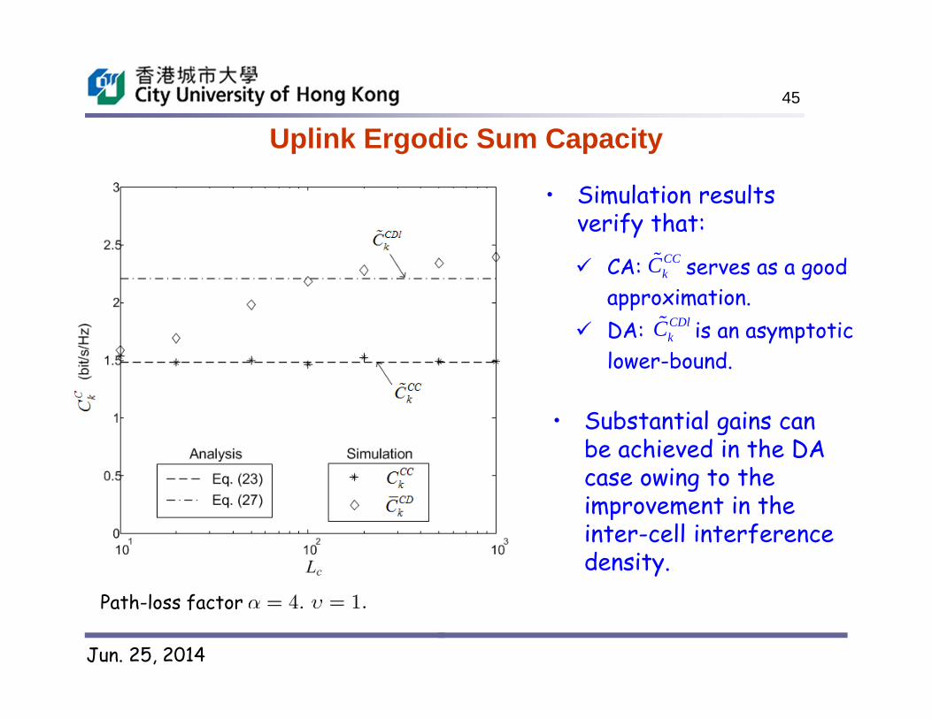
Uplink Ergodic Sum Capacity
• Simulation results verify that:
• Substantial gains can be achieved in the DA case owing to the improvement in the inter-cell interference density.
DA: is an asymptotic lower-bound.
CA: serves as a good approximation.
45
Path-loss factor
CCkC
CDlkC

Jun. 25, 2014
46
Sum Rate with Orthogonal Access

Jun. 25, 2014
Sum Rate with Orthogonal Access
• Normalized sum rate with orthogonal access:
47
CA:
as and
for large and : A significant tradeoff has to be made between complexity and performance if each cell has a large number of BS antennas and users.
• For large and :
DA:
Both and logarithmically increase with because and .
Jun. 25, 2014
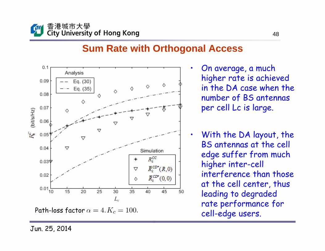
Sum Rate with Orthogonal Access
• On average, a much higher rate is achieved in the DA case when the number of BS antennas per cell Lc is large.
48
Path-loss factor
• With the DA layout, the BS antennas at the cell edge suffer from much higher inter-cell interference than those at the cell center, thus leading to degraded rate performance for cell-edge users.
Jun. 25, 2014
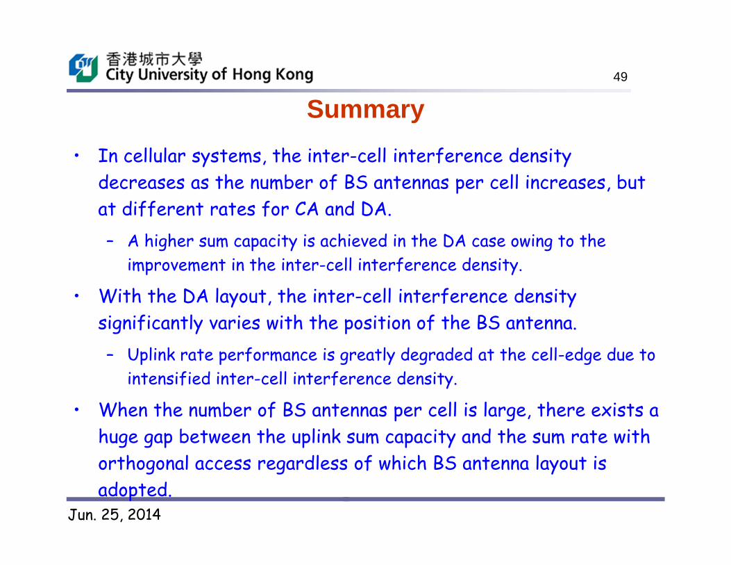
Summary• In cellular systems, the inter-cell interference density
decreases as the number of BS antennas per cell increases, but at different rates for CA and DA. – A higher sum capacity is achieved in the DA case owing to the
improvement in the inter-cell interference density.
• With the DA layout, the inter-cell interference density significantly varies with the position of the BS antenna.– Uplink rate performance is greatly degraded at the cell-edge due to
intensified inter-cell interference density.
• When the number of BS antennas per cell is large, there exists a huge gap between the uplink sum capacity and the sum rate with orthogonal access regardless of which BS antenna layout is adopted.
49
Jun. 25, 2014
50
Part III. DAS with Virtual Cells
• Virtual cell
• Inter-cell interference density
• Sum capacity and sum rate with orthogonal access

Jun. 25, 2014
To Cellular or Not to Cellular?51
• By splitting a large area into small ones, there are always a certain number of users/BS antennas located at the border and closer to the neighboring cells.
• With distributed BS antennas, the geographic division of cells becomes less justified.

Jun. 25, 2014
Virtual Cell52
• Each user chooses a few surrounding BS antennas as its virtual cell [1-3], i.e., its own serving BS antenna set.
• Different from the conventional cellular structure where cells are divided according to the coverage of BS antennas, here the virtual cell is formed in a user-centric manner.
• For user k, define its virtual cell as a set of BS antennas with the largest large-scale fading gains to this user.
[1] L. Dai, Researches on Capacity and Key Techniques of Distributed Wireless Communication Systems, Ph.D. Dissertation, Tsinghua University, Beijing, Dec. 2002.[2] L. Dai, S. Zhou, and Y. Yao, ``Capacity with MRC-based Macrodiversity in CDMA Distributed Antenna Systems,'' in Proc. IEEE Globecom, pp. 987--991, Nov. 2002.[3] L. Dai, S. Zhou, and Y. Yao, ``Capacity Analysis in CDMA Distributed Antenna Systems,'' IEEE Trans. Wireless Commun., vol. 4, no. 6, pp. 2613--2620, Nov. 2005.

Jun. 25, 2014
Signal Model
• Received signal of Virtual Cell :
: The set of users whose signals are jointly processed with user k’s at virtual cell .
• Uplink power control:
53
Inter-cell interference
•
• is defined as the set of users whose virtual cells are overlapped with , i.e., iff

Jun. 25, 2014
54
Inter-cell Interference Density

Jun. 25, 2014
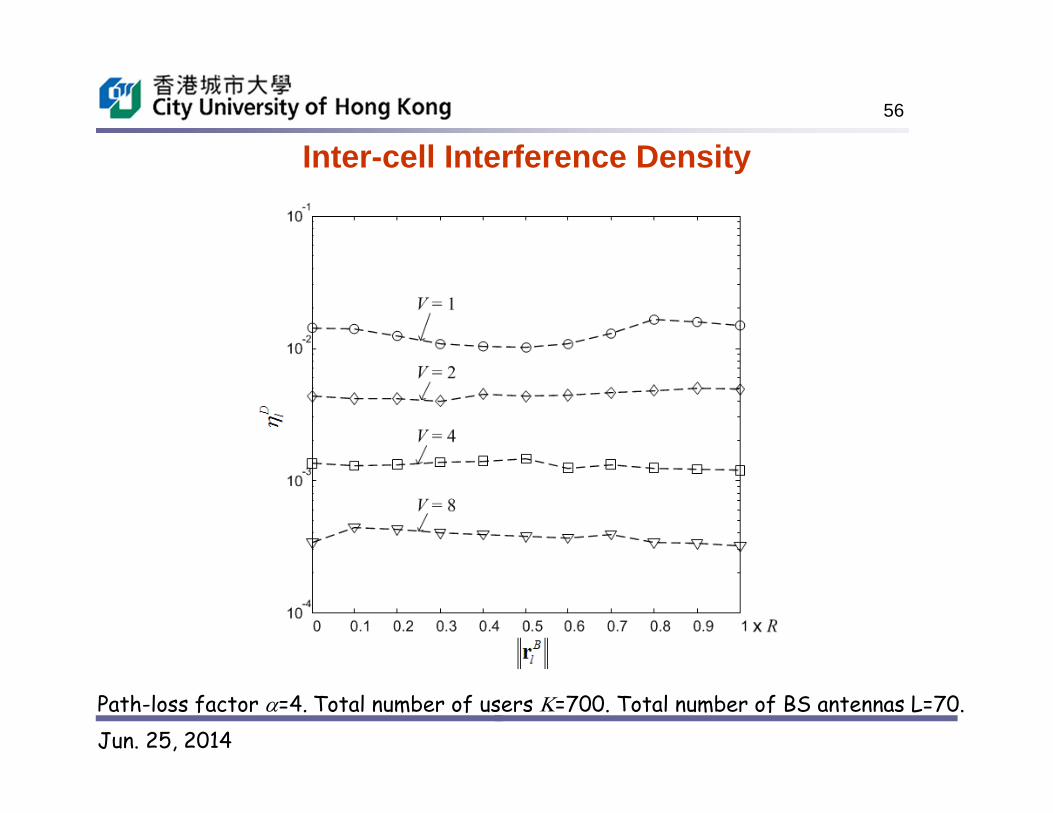
Inter-cell Interference Density55
• Inter-cell interference density of BS antenna
Compared to the cellular system:
• Key difference of and lies in the division of cells:
consists of users who fall into the cell centered at BS 1. consists of users whose virtual cells are overlapped with .
Jun. 25, 2014
Inter-cell Interference Density
Path-loss factor =4.
56
Total number of users =700. Total number of BS antennas L=70.

Jun. 25, 2014
Average Inter-cell Interference Density57
• Average inter-cell interference density
• Theorem 3. The average inter-cell interference density of BS antenna l at in DASs with V=1 is

Jun. 25, 2014
Average Inter-cell Interference Density
Path-loss factor =4.
58
, 1 1D Vl L
Compared to cellular systems with the DA layout, the average inter-cell interference density with V=1 has a smaller decreasing rate with the number of BS antennas L because the interfering area increases with L.
For cellular systems:
/2CDul cL
1CCl cL
, 1D Vl
The average number of intra-cell users 1 / .V
l K L
Jun. 25, 2014
59
Sum Capacity and Sum Rate with Orthogonal Access

Jun. 25, 2014
Uplink Ergodic Sum Capacity with V=1
• Normalized sum capacity:
60
: number of intra-cell users
: average received SINR of BS antenna
• Lower-bound for the average normalized sum capacity :
For large and :

Jun. 25, 2014
Sum Rate with Orthogonal Access with V=161
• Normalized sum rate with orthogonal access:
• Lower-bound for the average sum rate :
For large and :

Jun. 25, 2014
Sum Capacity and Sum Rate
• Both and linearly increase with the number of BS antennas L.
62
Path-loss factor
• A small gap between and is observed ----by the use of virtual cell, the average number of users served by each BS antenna decreases as L increases!
• With V=1, the DAS suffers from severe inter-cell interference.
DkC D
kR
DkC
DkR

Jun. 25, 2014
Implications to Cutting-edge Cellular Technologies
• Cellular Systems with Small Cells
– Equivalent to a DAS with V=1.
– Sum capacity is lower than that of cellular systems with co-located BS antennas due to strong inter-cell interference.
– To improve the sum capacity:
• Cooperation should be adopted among BSs, and
• The cooperative BS set should be formed in a user-centric manner ---- virtual cell.
63
Jun. 25, 2014
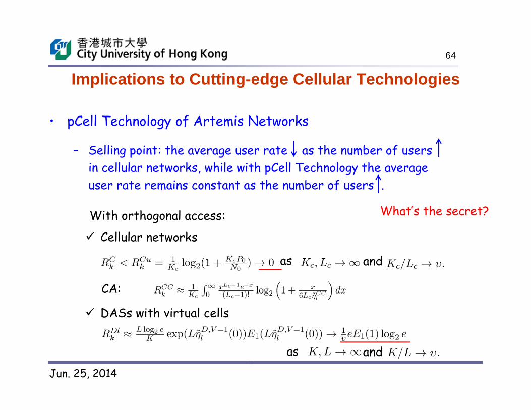
Implications to Cutting-edge Cellular Technologies 64
• pCell Technology of Artemis Networks
– Selling point: the average user rate as the number of users in cellular networks, while with pCell Technology the average user rate remains constant as the number of users .
CA:
Cellular networks
as and
DASs with virtual cells
as and
What’s the secret?With orthogonal access:

Jun. 25, 2014
Summary• In a DAS, if each user chooses a few surrounding BS antennas to
form its virtual cell:– A uniform inter-cell interference density can be achieved.
– Each BS antenna serves a declining number of users as the density of BS antennas increases, indicating good network scalability.
– A small gap between the sum capacity and the sum rate with orthogonal access with V=1 is observed, which is in sharp contrast to cellular systems where a significant tradeoff between performance and complexity has to be made when the number of BS antennas is large.
65
• The size of virtual cell V is a crucial system parameter.– How does the sum capacity vary with V?

Jun. 25, 2014
Thank you!
Any Questions?
66
Slides can be downloaded at my homepage: http://www.ee.cityu.edu.hk/~lindai