on sequential data assimilation for scalar macroscopic traffic flow
TRANSCRIPT

Physica D 241 (2012) 1421–1440
Contents lists available at SciVerse ScienceDirect
Physica D
journal homepage: www.elsevier.com/locate/physd
On sequential data assimilation for scalar macroscopic traffic flow modelsSébastien Blandin a,∗, Adrien Couque b, Alexandre Bayen c,a, Daniel Work d
a IBM Research Collaboratory – Singapore, Singaporeb California Center for Innovative Transportation, United Statesc Systems Engineering, Department of Electrical Engineering and Computer Sciences, University of California, Berkeley, United Statesd Department of Civil and Environmental Engineering, University of Illinois at Urbana-Champaign, United States
a r t i c l e i n f o
Article history:Received 30 August 2011Received in revised form12 April 2012Accepted 14 May 2012Available online 22 May 2012Communicated by H.A. Dijkstra
Keywords:Traffic flowMacroscopic modelingSequential estimationData assimilationConservation lawRiemann problem
a b s t r a c t
We consider the problem of sequential data assimilation for transportation networks using optimalfiltering with a scalar macroscopic traffic flow model. Properties of the distribution of the uncertainty onthe true state related to the specific nonlinearity and non-differentiability inherent to macroscopic trafficflow models are investigated, derived analytically and analyzed. We show that nonlinear dynamics, bycreating discontinuities in the traffic state, affect the performances of classical filters and in particularthat the distribution of the uncertainty on the traffic state at shock waves is a mixture distribution. Thenon-differentiability of traffic dynamics around stationary shock waves is also proved and the resultingoptimality loss of the estimates is quantified numerically. The properties of the estimates are explicitlystudied for the Godunov scheme (and thus the Cell-Transmission Model), leading to specific conclusionsabout their use in the context of filtering, which is a significant contribution of this article. Analyticalproofs and numerical tests are introduced to support the results presented. A Java implementation of theclassical filters used in this work is available on-line at http://traffic.berkeley.edu for facilitating furtherefforts on this topic and fostering reproducible research.
© 2012 Elsevier B.V. All rights reserved.
1. Introduction
1.1. Motivation
At the age of ubiquitous sensing, scientists and engineersare faced with the challenge of leveraging massive cross-domaindatasets to solve increasingly complex problems and addresssystemic issues at unprecedented scales [1]. In transportationnetworks, the spread of crowd-sourced traffic data is revolutioniz-ing traffic data collection. In parallel, the democratization of pub-licly available and easily accessible high performance computingresources offers scalable tools for massive data processing. Thisconjunction of factors is accelerating the pace of development andimplementation of novel on-line traffic estimation methods andfiltering algorithms, from which real-time congestion controlstrategies may be designed at the scale of mega-cities.
The theory of estimation is concerned with the problem ofproviding statistics of a process state, based onmeasurements and
∗ Correspondence to: IBM Singapore Pte Ltd, 9 Changi Business Park Central 1,The IBM Place, Singapore 486048, Singapore.
E-mail addresses: [email protected] (S. Blandin),[email protected] (A. Couque), [email protected] (A. Bayen),[email protected] (D. Work).
0167-2789/$ – see front matter© 2012 Elsevier B.V. All rights reserved.doi:10.1016/j.physd.2012.05.005
a priori knowledge. The a priori knowledge of the process oftenconsists of a parametric model, which approximately describesthe process behavior mathematically. The definition of a lossfunction allows for the formulation of the estimation problemas an optimization problem and the identification of certificatesof optimality. When the estimated quantities are not directlyobserved, (so-called latent variables) the estimation problem isreferred to as an inverse problem [2]. For physical systems, theestimation problem, or data assimilation problem [3,4], is solvedusing a data assimilation algorithm, which combines optimally,in the sense of the loss function, the a priori knowledge of thesystem, and the observations from the system. In particular, afiltering algorithm provides the solution to an inverse problemwhich includes the additional constraint that, for all times t , onlyobservations at or before time t can be used to compute estimatesat time t .
The basis for modern filtering theory was set by Kalman in1960 who introduced a sequential filtering algorithm for lineardynamical systems, the Kalman filter (KF) [5]. This algorithmextended the work of Wiener [6] and proposed one of the firstresults on optimal filtering for linear dynamical systems withnon-stationary statistics. The KF sequentially computes the bestestimate of the true state of a system from combined knowledgeof a model and observations. The KF has been widely applied bythe control community, notably to signal processing, sensor datafusion, navigation and guidance [7,8].

1422 S. Blandin et al. / Physica D 241 (2012) 1421–1440
In the meteorology community, the estimation problem fornonlinear systems has been heavily studied, with subsequentdevelopment of sophisticated data assimilation techniques [3,4],which fall into two major categories: variational methods andoptimal interpolation methods. Variational methods [4] consistof finding the solution of a model (with or without stochasticforcing) which minimizes a certain distance to observations. Inmeteorology, a common formulation is the 3D-Var algorithm [9]for the static problem and 4D-Var algorithm in the time-varyingcase [10].
The need for solving the inverse problem for increasingly com-plex systems, for which the classical assumptions of linearity ofthe dynamics and normality of the error terms break, has moti-vated the development of suboptimal sequential estimation algo-rithms. Suboptimal sequential estimation algorithms, reviewed inSections 2.2 and 2.3, can be derived from the KF by different typesof methods:
1. Deterministic filters: extended Kalman filter (EKF) [11], unscentedKalman filter (UKF) [12].
2. Stochastic filters: ensemble Kalman filter (EnKF) [13], particlefilter (PF) [14].
For traffic applications, it is also important to mention themixtureKalman filter (MKF) [15], which provides optimality guaranteesfor conditionally linear systems. A comprehensive review of theapplication of data assimilation algorithms in the transportationcommunity can be found in the following section.
1.2. Sequential estimation for transportation networks
Sequential traffic state estimation dates back to the 1970s andthe work of Gazis [16,17], who independently used the KF andthe EKF to estimate traffic density in the Lincoln tunnel, NewYork, for the purpose of traffic control. More recent work fromPapageorgiou [18,19] involves the application of the EKF to a non-scalar traffic model [20]. The EKF has also been applied [21] to theLWR equation with a Smulders [22] flux function.
The MKF [15] is an extension of the KF to conditionally lin-ear dynamical systems. The MKF has been applied in the trans-portation community [23–25] to the cell-transmission model (CTM)[26,27], which exhibits piecewise linear dynamics, conditioned onthe phases of traffic (free-flow, congestion) upstream and down-stream.
In recent years, sequential Monte Carlo methods, or PF, andso-called ensemble methods such as the EnKF have been appliedto traffic estimation [28,29]. Ensemble methods [13] consist ofrepresenting the first moment of the state estimate distributionby a set of samples and using a linear measurement update,whereas particle methods [30] consist in propagating a samplerepresentation of the full distribution of the estimate and using anonlinear measurement update.
Another notable filter is the UKF [12] which introduces anunscented transformation providing an exact representation of thefirst two moments of a distribution by a set of deterministicallydetermined samples (see [31] for a traffic application).
A variety of traffic models and filters have been shown toperform well for practical applications. However, the problem ofthe structural limits of data assimilation algorithms for trafficestimation has not received much attention. It is well knownthat, in practice, high accuracy can be achieved with sufficientlyaccurate measurements in sufficiently large volumes. But withmassive datasets coming from increasingly diverse sources,traceability and high quality of traffic data are not necessarilyguaranteed. Being able to identify the estimation errors inherentto the structure of traffic phenomena is required for the design
of more robust, transparent data assimilation algorithms, andscalable, appropriate data collection methodologies.
In this article, we propose to analyze the structural proper-ties of one of the most classical macroscopic traffic flow models,the Lighthill–Whitham–Richards (LWR) partial differential equation(PDE) [32,33], in the context of estimation. We present the dif-ficulties resulting from these properties, which create significantchallenges for the design of an optimal filtering algorithm for thismodel. Themain contributions of the article are outlined in the fol-lowing section.
1.3. Optimal filtering for LWR PDE
Structural properties of the LWR PDE and its discretized formsimpact the optimality of estimates produced by classical sequentialestimation techniques. The main contributions of this article arethe analysis and quantification of the lack of estimate optimalityresulting from the following properties of the LWR PDE, and itsnumerical discretization using the Godunov scheme:Nonlinearity of the fundamental diagram
One of the main properties of the LWR PDE is the nonlinear-ity of its flux function (fundamental diagram), which allows themodeling of traffic phases of different nature: free-flow and conges-tion. Nonlinearities of themodel are the cause of the appearance ofdiscontinuities in the solution of the partial differential equation.Consequently, the distribution of the uncertainty on the true stateis a mixture distribution at shock waves even for unimodal noisedistributions on the initial condition. In this article, we analyticallyshow the emergence of mixture distributions in the solution ofthe PDE and numerically illustrate their importance on benchmarktests.
Themixture nature of the distribution of the uncertainty on thetrue state resulting from initial condition uncertainty propagatingthrough an uncertain model raises the question of the relevanceof minimal variance estimate for traffic applications. The estimateproduced by classical filters may indeed correspond to a state withzero true probability, and the estimate covariance may exhibitlarge values corresponding to a variability due to the coexistenceof differentmodes in the distribution of the uncertainty on the truestate, each with significantly smaller covariance.Non-differentiability of the discretized model
The most common numerical scheme used to compute thesolution of the LWRPDE is theGodunov scheme [34], a finite volumeschemewhich consists of iteratively solving Riemann problems [35]between neighboring discretization cells and averaging theirsolution at each time-step on each spatial cell. In this articlewe prove that this scheme is non-differentiable and derive theexpression of its non-differentiability domain.
The lack of differentiability of the Godunov scheme, a commondiscretization of the LWR PDE, is relevant for data assimilationalgorithmswhose optimality guarantees are based on Taylor seriesanalysis, which assumes exact computation of the derivative upto a certain order. This is the case in particular for the EKF,which considers propagation of the estimate covariance using thetangent (linearized) model. Numerical results quantify estimateerrors induced by this property of the discretizedmodel. The resultalso affects the known order of accuracy of the estimate momentsof the UKF, since in this case the Taylor series does not exist up tothe required order.
This article can thus be viewed as a theoretical and numericalstudy of the implications of the structural properties of theGodunov scheme and CTM on filtering algorithms. It sheds somenew light on the proper use of these schemes for traffic estimationpurposes, and provides conclusions which are illustrated bydetailed numerical studies.

S. Blandin et al. / Physica D 241 (2012) 1421–1440 1423
While the results presented in this article are derived forthe Godunov scheme, because historically is was one of thefirst numerical schemes proposed to solve scalar hyperbolicconservation laws (and the LWR PDE in particular), other proposedschemes such as the CTMexhibit the same features as the Godunovscheme, and thus our analysis applies to them as well.
The remainder of the article is organized as follows. Section 2introduces the general theory of sequential data assimilation andoptimal filtering. In Section 3wepresent themost classical discreteand continuous macroscopic traffic models for which the studyis conducted. Section 4 focuses on the Riemann problem which isthe keystone of numerical solutions of continuous and discretescalar conservation models and the focus of our subsequentanalysis. Sections 5 and 6 point at the structural properties ofmacroscopic trafficmodels derived from the LWRPDE, in particularmodel nonlinearity in Section 5 and model non-differentiabilityin Section 6. Section 7 gives concluding remarks and examinesassociated issues regarding data fusion.
2. Sequential data assimilation
The theory of inverse problems [2] is concerned with theestimation of model parameters. A specific type of inverse methodsconsists in iteratively updating the estimates as data becomesavailable [36], instead of solving an inverse problem once usingall measurements in batch. These so-called sequential estimationalgorithms, particularly appropriate for on-line estimation, oftenrely on Bayes’ rule and a computationally explicit optimalitycriterion (e.g. the Gauss–Markov theorem for minimum meansquared error (MMSE) estimation). In the case of additive noise,one of the most well-known sequential estimation algorithms isthe seminal Kalman filter [5].
2.1. Kalman filter
Given a system with true state at time t denoted by Ψt , and Ytthe vector of all available observations up to time t , the filteringproblem is concerned with the computation of an optimal estimateof Ψt for a predefined loss function. Solvability of the estimationproblem heavily depends on the loss function used, and on thestatistics considered.
The use of the quadratic loss function dates back to theestimation problem posed by Gauss in the 18th century forastronomy [37,38]. The solution proposed by Gauss is the so-calledleast-squares method, justified by the Gauss–Markov theorem [39].The theorem proves that, assuming a linear observation modelwith additive white noise, the best linear unbiased estimator (BLUE)(best in the minimum variance sense), of a random processψt canbe computed as the solution to the ordinary least squares (OLS)problem.
The role of the quadratic norm for estimation is furtheremphasized by a result from Sherman [40], which shows thatfor a large class of loss functions, which includes the quadraticloss function, the mean of the conditional distribution p(ψt |Yt) isoptimal.
Formally, given a loss function L(·) such that:
L(0) = 0∃ f real-valued convex s.t. ∀ψ1, ψ2 s.t. f (ψ1) ≥ f (ψ2)
then L(ψ1) ≥ L(ψ2),
(1)
given a random variable ψ , if the probability density functionassociated with the random variable ψ is symmetric around themean, and unimodal, then E(ψ) is the optimal estimator of ψ forthe loss function L(·).
When applied to the conditional random variable ψt |Yt , thisshows that the conditional mean is the optimal estimator in thesense of the loss function L(·) for this particular class of lossfunctions and probabilities.
The statistical assumptions on the processes ψt and Yt are tiedto prior knowledge of the generative distributions. However, asignificant computational argument in favor of the use of normalstatistics is the optimality guarantee provided by combining thetwo arguments above. Without any assumption on the statistics,the Gauss–Markov theorem states that the BLUE is given by thesolution to the OLS algorithm. Sherman’s result (1) states that thesolution of theOLS is the conditionalmean. In theGaussian case theconditional mean is linear, hence it is also the solution of the OLSwith constraint that the estimator be linear. Hence the BLUE of theprocess is optimal, without restriction of linearity on the estimator,if we assume that the statistics are Gaussian.
In his seminal paper [5], Kalman provides a sequentialalgorithm to compute the BLUE of the state for dynamical systems,under additive white Gaussian noise, with a deterministic linearobservation equation (this result was later extended to includeadditive white Gaussian observation noise). The KF is defined ina state-space model, which consists of a state equation and anobservation equation. In the following, we denote by xt the state attime t , a discrete computable approximation of the deterministictrue state Ψt .
For transportation applications involving macroscopic vari-ables, the state is typically a set of densities, speeds, or counts, de-fined on a discretization grid. The true state consists of the truetraffic conditions on the road, which are only available to an oracle,or some high fidelity datasets such as the NGSIM dataset [41]. Forsimulation purposes, it is common practice to use awell-calibratedmodel, or a Monte Carlo simulation with high number of samples,as a proxy for the true state (to avoid the so-called inverse crime [2],the model used for estimation should be different from the modelused for computing the true state).
We consider the following discrete linear model:
xt = At xt−1 + wt (2)
where we denote by At the state model or time-varying statetransition matrix at time t , and where the random variable wt ∼
N (0,Wt) is a white noise vector which accounts for modelingerrors. In particular in this setting the true state Ψt is assumed tofollow the dynamics At without additional noise. Measurementsare modeled by the linear observation equation:
yt = Ct Ψt + vt (3)
where vt ∼ N (0, Vt) is a white noise vector which accounts formeasurement errors assumed uncorrelated with modeling errors,and Ct is the modeled measurement matrix at time t (also time-varying, to integrate the possibility of moving or intermittentsensors). The KF sequentially computes the BLUE at time t+1 fromthe BLUE at time t as follows:
Forecast:xt+1|t = At+1 xt|tΣt+1|t = At+1Σt|t AT
t+1 + Wt+1(4)
Analysis:
xt+1|t+1 = xt+1|t + Kt+1
yt+1 − Ct+1 xt+1|t
Σt+1|t+1 = Σt+1|t − Kt+1 Ct+1Σt+1|t
where Kt+1 = Σt+1|t CTt+1
Ct+1Σt+1|t CT
t+1 + Vt+1−1
.
(5)
The forecast step (4) consists in propagating the mean andcovariance of the state through the linear model (2). The analysisstep (5) amounts to the computation of the conditionalmean of thestate given the observations, for the linear observation model (3)and jointly Gaussian statistics. The conditional covariance iscomputed similarly. From a Bayesian perspective, the Kalman filter

1424 S. Blandin et al. / Physica D 241 (2012) 1421–1440
sequentially computes the posterior distribution of the state, basedon the prior distribution given by the state-space model.
When the statemodel is not linear, there is no general analyticalexpression for the propagation of the statistics. Suboptimal filtersof different types have been derived. Stochastic methods considerpropagating the state through the nonlinear model using a samplerepresentation. Deterministic methods consist in propagatinganalytical approximations of low order moments through themodel. Stochastic methods require in general sampling schemesand pseudo-random generators for the correct execution of thefilters, unlike deterministic methods.
2.2. Deterministic filters
In this section we present the EKF and the UKF for nonlinearsystems. The EKF forecast step is based onmodel linearization. TheUKF consists in representing exactly the first two moments of theprior distribution by a set of deterministic samples. In particular, nosampling term is required for the application of these algorithms.
2.2.1. Extended Kalman filterThe EKF is an extension of the KF for nonlinear state-space
models. The EKF consists in using a Taylor series truncation ofthe model at the current state to propagate the state statistics.We present the case of a nonlinear state model combined witha linear observation model, although a nonlinear observationequation can also be considered through a similar linearization ofthe observation operator at the analysis step. The forecast mean isgiven by the nonlinear model, whereas the forecast covariance isgiven by a first order approximation of the model. If we denote byAt+1 the linearization of the nonlinear model dynamics A(·, t) atthe state estimate xt|t , the forecast and analysis steps for the EKFread:
Forecast:xt+1|t = A(xt|t , t)Σt+1|t = At+1Σt|t AT
t+1 + Wt+1(6)
Analysis:
xt+1|t+1 = xt+1|t + Kt+1
yt+1 − Ct+1 xt+1|t
Σt+1|t+1 = Σt+1|t − Kt+1 Ct+1Σt+1|t
where Kt+1 = Σt+1|t CTt+1
Ct+1Σt+1|t CT
t+1 + Vt+1−1
(7)
where the only difference from the Kalman filter resides in thepropagation of the state mean at the forecast step, using thenonlinear state model. Different sources of sub-optimality arise inthe derivation of the EKF:
1. Accuracy of the Taylor truncation:a The model approximation used at the forecast step (6) forthe covariance propagation requires that the model Jacobianbe accurately computed.
b The mean given by the EKF is a first order Taylor seriesapproximation of theMMSE,whereas the covariance is a thirdorder approximation of the MMSE covariance.
2. Closure assumption: it is assumed that there is no significantinteraction between higher order statistics and the first twomoments of the state estimate.
Cases in which the closure assumption breaks, due to theimportance of higher order terms in the model Taylor serieshave been documented, with illustrations of estimates biased andinconsistent [12], and with diverging error statistics [42]. Cases inwhich this assumption breaks, due to the importance of higher-order statistics can be found in [43,44] in the case of bimodaldistributions.
Remark 1. An approximationmade in the EKF equations lies in thepropagation of the state covarianceΣt+1|t . This covariance is thenused at the analysis step (7) at which observations are combined
with the model forecast. The study of the resulting error structureof the state covariance after propagation in the context of traffic isto the best of our knowledge an open problem, and is a focus of thisarticle.
2.2.2. Unscented Kalman filterThe UKF [12] is built on the unscented transformation, which
consists in representing a distribution with mean µ and varianceΣ by a set of weighted samples, or sigma points, chosen determin-istically such that theweighted samplemean isµ and theweightedsample covariance isΣ [45]. For a state-space of dimension n, the2 n+1 sigma points produced by the unscented transformation aredefined as
x0 = µ
xk = µ+ ((n + κ)Σ)12k k = 1, . . . , n
xk+n= µ− ((n + κ)Σ)
12k k = 1, . . . , n
(8)
where ((n + κ)Σ)1/2k denotes the kth column of the square root of
(n + κ)Σ . The corresponding weightswk are parameterized by κ ,which controls the spread of the sigma points:w0
=κ
κ + nwk
=1
2(κ + n)k = 1, . . . , n
wk+n=
12(κ + n)
k = 1, . . . , n.
(9)
Choosing the samples according to (8) and the weights accordingto (9) yields that the weighted sample mean and weighted samplecovariance are equal to the distribution mean and covariance forany choice of κ . The forecast and analysis step of the augmentedUKF [46] can be written as:
Forecast:
Propagate sigma-pointsxkt+1|t = A(xkt|t , t) k = 0, . . . , 2 n
Compute forecast mean and covariance
xt+1|t =
2 nk=0
wk xkt+1|t
Σt+1|t =
2 nk=0
wkxkt+1|t − xt+1|t
xkt+1|t − xt+1|t
T(10)
Analysis:
Compute sigma-points observationszkt+1|t = Ct+1 xkt+1|t k = 0, . . . , 2 n
Compute observation mean and covariance
zt+1|t =
2 nk=0
wk zkt+1|t
Zt+1|t =
2 nk=0
wkzkt+1|t − zt+1|t
zkt+1|t − zt+1|t
TCompute covariance between forecast and observation
Yt+1|t =
2 nk=0
wkxkt+1|t − xt+1|t
zkt+1|t − zt+1|t
TCompute posterior mean and covariance
xt+1|t+1 = xt+1|t + Kt+1yt+1 − zt+1|t
Σt+1|t+1 = Σt+1|t − Kt+1 Zt+1|t K T
t+1where Kt+1 = Yt+1|t Z−1
t+1|t
(11)
where the unscented transformation is first used to compute thesigma points for the current estimates, which are then propa-gated through the model and whose mean and covariance is com-puted (10). At the analysis step, the forecast observation associated
S. Blandin et al. / Physica D 241 (2012) 1421–1440 1425
with each sigma point through the (potentially) nonlinear obser-vation model Ct+1, is computed as zkt+1|t , which allows the com-putation of the observation mean zt+1|t , observation covarianceZt+1|t , and the covariance between forecast state and observationas Yt+1|t . The analysis mean and covariance are then computed ex-actly using Kalman equations (11).
Different sources of sub-optimality arise in the UKF:
1. Limited number of samples: the mean and the covariancepropagated by the UKF are third order approximations of theMMSE and MMSE covariance.
2. Closure assumption: it is assumed that there is no significantinteraction between higher order statistics and the first twomoments of the state estimate.
The UKF has been applied to traffic estimation [31] and wascompared with the EKF for the Papageorgiou model (23). The twofilters were empirically shown to have similar performances forjoint state and parameter estimation [46] for this model (23). Theresults of this comparison are completed by the analysis presentedin the present article in Sections 5 and 6, in which we study thestate distribution features due to model nonlinearities and non-differentiability analytically andnumerically in the case of the LWRmodel, and in which we show how they affect the EKF and theUKF. In particular we analyze the true distribution structure atshock waves of the LWR model, in the continuous and discretedomain. The Papageorgioumodel is defined in the discrete domain,and exhibits an anticipation term which reduces the sharpnessand amplitude of spatial variations. Consequently, the impact ofthe existence of shock waves on the performance of the filters isstronger in the case of the LWR model in the continuous domain,as illustrated in the present article.
2.3. Stochastic filters
A wide variety of filters extend the Kalman filter for nonlinearstate models by representing the state by a set of random samples(particles, ensemble members). The rules for sample propagation,update, and for resampling, are of different types. The needfor pseudo-random generator at every step of these algorithmsjustifies the appellation stochastic filters.
2.3.1. Ensemble Kalman filterThe EnKF [47,13] consists in representing the state statistics
by a set of ensemble members which are evolved in time andwhose mean is an estimator of the true state. The state errorcovariance is represented by the ensemble covariance. Formally,with N ensemble members, the EnKF equations read:
Forecast:
xkt+1|t = A(xkt|t , t)+ wkt+1 k = 1, . . . ,N
xt+1|t =1N
Nk=1
xkt+1|t
Σt+1|t =1
N − 1
Nk=1
xkt+1|t − xt+1|t
xkt+1|t − xt+1|t
T (12)
Analysis:xkt+1|t+1 = xkt+1|t + Kt+1yt+1 + vkt+1 − Ct+1 xkt+1|t
k = 1, . . . ,N
Σt+1|t+1 = Σt+1|t − Kt+1 Ct+1 Σt+1|t
where Kt+1 = Σt+1|t CTt+1
Ct+1 Σt+1|t CT
t+1 + Vt+1−1
.
(13)
In the limit of large number of samples, the EnKF convergestoward the KF for linear systems. Due to the independent ensembleforecasts (12), it is embarrassingly parallel and particularlyappropriate for efficient distributed computations. At the analysisstep (13), the modeled observation noise is explicitly added to the
measured observation, to capture the full observation noise in theanalysis equation [48]. In the context of traffic estimation, the EnKFhas been applied to the Bay Area highway networks with a trafficmodel equivalent to the LWR PDE, formulated using a velocityvariable [29]. The principal source of sub-optimality arising in theEnKF is sampling error:
1. Sampling error: the use of a finite number of ensemblemembersintroduces a sampling error in the estimate distribution.
Remark 2. The covariance given by the EnKF is the state errorcovariance and not the state covariance. In the KF, the state meanand state error covariance are propagated analytically. The stateerror covariance coincides with the state covariance. On the otherhand, the EnKF analytically propagates ensemble members whosemean is an unbiased estimator of the state mean, and covariancecoincides by definition of the update equationswith the state errorcovariance, but not with the state covariance, except in the limit ofan infinite number of ensemble members.
Extensions of the EnKF allowing to obtain higher ordermoments ofthe state distribution have also been considered [49] by integratinga modified analysis step.
2.3.2. Particle filterThe PF, also known as bootstrap filter, or sequential Monte Carlo
method [50,30,14] can be traced back to the seminal articles ofMetropolis andUlam [51], later generalized byHastings [52]. Thesemethods represent the full statistics of the state by a set of sampleswhich are propagated through the statemodel.When observationsare received, sample weights are scaled by the relative likelihoodof the new observation, and the updated representation of theprobability distribution is re-sampled. Formally, the PF steps in thecase of N particles are as follows:
Forecast: xkt+1|t = A(xkt|t , t)+ wkt+1 k = 1, . . . ,N
Analysis:
Re-weighting:
αkt+1 = αk
t
p(yt+1|xkt+1|t)
Nk=1αkt p(yt+1|xkt+1|t)
k = 1, . . . ,N
Re-sampling:Generate N samples xkt+1|t+1from the distribution defined byP(X = xkt+1|t+1) = αk
t+1, k = 1, . . . ,N.
The PF has been applied to the case of transportation systems [28]on the stochastic model described in [53]. The particle filter isthe only filtering method able to capture the complete statedistribution, in the limit of infinite number of samples, withoutrestrictive assumption on the dynamics or on the statistics. Well-known weaknesses of the PF relate to the problem of sampledegeneracy for high dimensional [54] systems. The use of anappropriate proposal distribution at the re-weighting step is keyto reducing the sample weight variance given the system history,but more sophisticated importance sampling or rejection samplingtechniques are often considered [50,55]. The sources of sub-optimality in the PF relate to:
1. Sampling error: the use of a finite number of particles introducesa sampling error in the estimate distribution.
The implicit particle filter is a notable extension [56] of the PFwhich allows a priori the definition of the desired weights ofthe particles after analysis and thus alleviation of the problem ofsample degeneracy in the case of the exponential family. Anotherresearch track has explored the use of the EKF, EnKF or UKF tocompute a proposal distribution in the particle filter [55].

1426 S. Blandin et al. / Physica D 241 (2012) 1421–1440
Fig. 1. Fundamental diagrams: Greenshields (left), triangular (center), exponential (right).
Sustained improvements of the filters presented above havebeen in large part driven by specific improvements for systemsexhibiting strong nonlinearity or non-normality, identified as thecauses of inaccurate estimates and forecast. In the followingsection, we present the seminal macroscopic traffic modelswhich have been considered for real-time data assimilation ontransportation networks. The subsequent sections will then focuson the analysis of the performance of the respective filteringschemes on the models, which is one of the contributions of thearticle.
3. Macroscopic traffic modeling
Macroscopic traffic modeling consists of considering trafficphenomena as a continuum of vehicles, instead of modelingindividual vehicle dynamics. Macroscopic traffic models arehistorically inspired from constitutive hydrodynamics models,which exhibit similar properties to traffic flow. In this section weintroduce one of the most common scalar traffic models, as well assome non-scalar models classically used for estimation.
3.1. Scalar models of traffic flow
Classical scalar models of traffic consider the traffic state at apoint x at time t to be fully represented by the density ρ(t, x)of vehicles at this point. The evolution of the density of vehiclescan be modeled by a combination of physical principles, statisticalproperties, and empirical findings. All the models considered inthis section are single-lane single-class models of traffic.
3.1.1. Continuous modelsA classical state equation used to model the evolution of the
density ρ(·, ·) of vehicles on the road network is the LWR PDE[32,33],which expresses the conservation of vehicles on road links:
∂tρ + ∂xQ (ρ) = 0 (14)
where the flux function Q (·), assumed to be space–time invarianton limited space–time domains, denotes the realized flux ofvehicles with the density ρ, at the stationary state. The fluxfunction, or fundamental diagram, is classically given by anempirical fit of the relation between density and flow. It can beequivalently given by an empirical fit V (·) of the relation betweendensity and space-mean speed, which allows us to define the fluxfunction as:
Q (ρ) = q = ρ v = ρ V (ρ),
where the central equality is a definition of the flow q. A varietyof parametric flux functions can be found in the literature. One ofthe earliest flux functions is the Greenshields flux function [57] orquadratic flux function (represented in Fig. 1, left), which expressesa linear relationship between density and speed, or equivalently aquadratic relation between density and flow:
Q (ρ) = vmax ρ
1 −
ρ
ρmax
(15)
where vmax denotes the free-flow speed and ρmax the jamdensity. The Newell–Daganzo flux function [27,58] or triangular fluxfunction, represented in Fig. 1, center, is a piecewise linear functionof the density, with different slopes in free-flow and congestion:
Q (ρ) =
ρ vmax if ρ ∈ [0, ρc]
ρc vmaxρmax − ρ
ρmax − ρcif ρ ∈ [ρc, ρmax]
(16)
where ρc denotes the critical density, which represents the densityat which the realized flow is maximal. The speed of backwardmoving waves in congestion is given byw = vmax ρc/(ρc − ρmax).Variations on a flux function based on an exponential relationbetween density and flow [59,20], parameterized by a, such as theone represented in Fig. 1, right, can be found in the literature:
Q (ρ) = ρ vmax exp
−1a
ρ
ρc
a. (17)
The interested reader might also consider the Greenberg funda-mental diagram [60] or the Van-Aerde fundamental diagram [61].
Remark 3. The LWR PDE models the evolution of traffic flowon a road segment with uniform topology. A junction is definedby a change of topology (crossing, number of lanes, speed limit,curvature, etc.) on a road segment, which requires specific effortsfor physical consistency and mathematical compatibility with thelink model. A junction can be modeled as a vertex of the graphrepresenting the road network. With each vertex is associatedan allocation matrix A, where aij expresses the proportion ofthe incoming flow from link j going to link i. For uniqueness ofthe solution of the junction problem, different conditions havebeen considered in the literature: for instance maximizing theincoming flow through the junction [62,27] or maximizing aconcave function of the incoming flow [63]. A formulation usinginternal dynamics for the junction [64] has been shown to beequivalent to the vertexmodels for themerge anddiverge junction.The interested reader is referred to the book by Garavello andPiccoli [65] for more details on the junction problem.
For traffic applications, given an initial condition ρ0(·) definedon a stretch [0, L], using the LWR model requires solving theassociated Cauchy problem, defined as the problem of existenceand uniqueness of a solution to the LWR PDE with initialcondition ρ0(·). If the initial condition is piecewise constant(which is the case for many numerical approximations) and self-similar,1the Cauchy problem reduces to the Riemann problem
1 A function f of n variables x1, . . . , xn is called self-similar if ∀α > 0 ∈
R, f (α x1, . . . , α xn) = f (x1, . . . , xn).

S. Blandin et al. / Physica D 241 (2012) 1421–1440 1427
(see Section 4.2). We focus our analysis for data assimilationon the Riemann problem, which, by its simplicity, allows fullanalytical and numerical characterization of the relation betweeninitial condition uncertainty and structure of the uncertainty in thesolution to the PDE.
3.1.2. Discretized link modelsGiven a discretization grid defined by a space-step 1x and
a time-step 1t , if we denote by ρni the discretized solution at
i1x, n1t and Cni the cell defined by Cn
i = [n1t, (n + 1)1t] ×
[i1x, (i + 1)1x], the discretization of the LWR PDE using theGodunov scheme [34] reads:
ρn+1i = ρn
i +1t1x
qG(ρn
i−1, ρni )− qG(ρn
i , ρni+1)
(18)
where the numerical Godunov flux qG(·, ·) is defined as follows fora concave flux function Q (·)with a maximum at ρc :
qG(ρl, ρr) =
Q (ρl) if ρr ≤ ρl < ρcQ (ρc) if ρr ≤ ρc ≤ ρlQ (ρr) if ρc < ρr ≤ ρlmin(Q (ρl),Q (ρr)) if ρl < ρr .
(19)
Remark 4. Another common scheme for hyperbolic conserva-tion laws is the random approximation scheme introduced byGlimm [66], which consists in constructing an approximate solu-tion by randomly sampling from the values of the solution in aneighborhood at the previous time step. For the sake of concision,the analysis in the present article is limited to finite volumemeth-ods, and the Godunov scheme in particular.
TheGodunov scheme is a first order finite volumediscretizationscheme commonly used for numerical computation of weakentropy solutions to one-dimensional conservations laws suchas the LWR PDE [67]. The design of the Godunov schemedynamics (18) results from the following steps:
1. At time n1t , for each couple of neighboring cells Cni , Cn
i+1,compute the solution to the Riemann problem defined at theintersection of cells Cn
i , Cni+1, by the left datum ρn
i and the rightdatum ρn
i+1.2. At time (n + 1)1t , on each domain {(n + 1)1t} × [i1x,(i+ 1)1x] compute the average of the solution of the Riemannproblem. Specifically, integrating the LWR PDE on the domainCn
i ,Cni
∂ρ
∂t+∂Q (ρ)∂x
dsdy = 0 (20)
and applying the Stokes theorem on Cni to this equality yields:
1x ρn+1i −
(n+1)1t
n1tQ (ρ(s, i1x))ds −1x ρn
i
+
(n+1)1t
n1tQ (ρ(s, (i + 1)1x))ds = 0, (21)
where we denote by ρn+1i the space average of the solution
to the Riemann problems on {(n + 1)1t} × [i1x, (i + 1)1x].Since the solution to the Riemann problems is auto-similar,hence constant at i1x and (i+ 1)1x, if we denote respectivelyby Q (ρn
i−1, ρni ), Q (ρ
ni , ρ
ni+1) the values of the corresponding
flow at these locations over the interval [n1t, (n + 1)1t], weobtain:
1x ρn+1i −1x ρn
i = 1t Q (ρni−1, ρ
ni )−1t Q (ρn
i , ρni+1),
which is the dynamics equation (18) of the Godunov scheme.
The first step of the Godunov scheme is exact whereas the secondstep, through averaging, introduces numerical diffusion (see [67]for more details). The consequence of this diffusion on estimationis further discussed in Section 5.
Remark 5. It must be noted that grid-free algorithms allow us tocompute numerical solutions of scalar conservation laws withoutnumerical diffusion [68], with a higher complexity in general. Inthe case of transportation, some algorithms have been shown tobe exact for specific fundamental diagrams and particular initialand boundary conditions [69–72].
The Godunov scheme has been shown to provide a numericalsolution consistent with classical traffic assumptions [73] and tobe equivalent to the supply–demand formulation for concave fluxfunctions with a single maximum. In the case of a triangular fluxfunction (16), the Godunov scheme reduces to the CTM [26,27]:
qG(ρl, ρr) = minρl V , ρc V , ρc V
ρmax − ρr
ρmax − ρc
,
which thus inherits the properties causing the filtering difficultiesmotivating the present article. The Godunov scheme (18) definesthe state equation used by the estimation algorithms fromSection 2. Analysis of the nonlinearity and non-differentiability ofthe Godunov scheme in the context of estimation are the subjectof Sections 5.2 and 6.
3.2. Non-scalar models of traffic flow
Non-scalar models of traffic flow consider additional state vari-ables and additional physical principles tomodel traffic states. Oneof the first non-scalar traffic flow models is the Payne–Whithammodel [74,75]:∂tρ + ∂xq = 0
∂tv + v vx +c20ρ∂xρ =
V (ρ)− v
τ.
(22)
The first equation expresses the conservation of vehicles, and thesecond equationmodels the evolution of speed, which is subject toconvection, anticipation, and relaxation (respectively second andthird left-hand side terms of second equation, and right-hand sideterm of the second equation).
The EKF has been applied to networks2 for state and parameterestimation [18,19], with the following discretization of thePayne–Whithammodel Eq. (22):
ρn+1i = ρn
i +1t1x
qni−1 − qni
vn+1i = vni +
1t1x
vnivni−1 − vni
+1tτ
V (ρn
i )− vni
−c20 1t1x
ρni+1 − ρn
i
ρni + κ
qni = ρni v
ni
(23)
where κ is a regularization parameter and the function V (·) isthe exponential fundamental diagram (17). Other notable modelswith two state variables (so-called second ordermodels) include theAw–Rasclemodel [76], the non-equilibriummodel [77], or the phasetransition model [78,79]. Traffic models with three state variableshave also been proposed [80] by addition of a state equation for thevariance.
In this article, we focus our analysis on scalar models andspecifically on nonlinearity and non-differentiability of the flow
2 For simplicity we omit the network terms (sources and sinks) in equation (23).

1428 S. Blandin et al. / Physica D 241 (2012) 1421–1440
associated with the Riemann problem, which is an exampleof a Cauchy problem representing the evolution of trafficdiscontinuities, which are critical for several applications (seefollowing Section 4.1). This applies on a case-by-case basis tohigher order models with similar features. The discrete secondorder model (23) is by definition unable to capture discontinuitiesexactly, and differentiable, however structural properties of thecontinuous Payne–Whitham model from which it is derivedexhibit similarities with the LWR model [81] and allow thegeneralization of some of our conclusions.
4. Discontinuities and uncertainty
At the macroscopic level, traffic flow exhibits nonlinearitieswhich can be modeled using nonlinear conservation laws such asthe LWR PDE (14). Nonlinearities are the cause for discontinuitieswhich may arise in finite time in the solution to the Cauchyproblem associated with the PDE even with smooth initial andboundary data. According to the definition of the solution to theRiemann problem (25), shock waves persist when, at a spatialdiscontinuity, the upstream density is lower than the downstreamdensity. Thus they cannot be neglected by any traffic application.Physically, these discontinuities model the existence of queues,which are one of the main foci of traffic flow research.
4.1. Estimation and control
Queue extremities are phenomena with very limited spatialextent, which characterize the interface between significantlydifferent phases of traffic flow. This propertymakes themrelativelyhard to directly measure and monitor using classical fixed sensinginfrastructure. This is especially truewhen the upstream end of thequeue is stationary, and can only be directly measured if it lies on afixed sensor or by probe vehicles reporting measurements exactlyat the corresponding location.
Large traffic variations occurring on a short spatial extent,typical of queue extremities, make them particularly hazardous,and being able to alert drivers of sudden changes in speed is oneof the focal points of traffic safety applications [82].
For control applications, accurately locating the location andpropagation speed of queues is critical. Their location typicallyimpacts ramp metering algorithms directly, since they are oftendesigned around the values of the upstream and downstreamflow at the upstream end of the queue. In the absence of sensors,the algorithm depends on the estimated flows upstream anddownstream of the ramp.
Furthermore, accurate estimation of the propagation speed ofqueues is one of the most essential components of traffic forecastand dynamic travel-time estimation. Estimating their propagationspeed requires the estimation of the left and right density atthe queue extremities, as well as accurate knowledge of thefundamental diagram.
In the context of model-based estimation, the influence ofmodel nonlinearity and non-differentiability on the quality of theestimates for traffic phenomena has not received much attentionin the traffic community with a few notable exceptions [46,83](see [84] for a related problem for atmospheric models, and [85]for a study of non-differentiability in a general context). In thefollowing section, we consider the Riemann problem, which is abenchmark problem for studying the solution to the LWR PDE, andthe evolution of shock waves. We then consider in Section 4.3 theRiemann problem with a stochastic datum, which is used in thefollowing sections as a framework for the study of the propagationof discontinuities in the presence of uncertainties.
4.2. Riemann problem
The Riemann problem is a Cauchy problem with a self-similarinitial condition, of the form:
ρ(t = 0, x) =
ρl if x < 0ρr if x > 0. (24)
The solution to the Riemann problem is the solution to theCauchy problem associated with the PDE with initial conditionthe Riemann datum (24). The Riemann problem is a key buildingblock for proofs of existence of solutions to the Cauchy problem forgeneral initial conditions in the space of bounded variations (BV),via Helly’s theorem [68]. It is also critical to the design of numericalschemes such as the wavefront tracking method [68] and theGodunov scheme, which proceeds by iteratively solving theRiemann problem between discretization cells, before averagingits solution on each cell (see Eqs. (20) and (21)).
For a flux functionQ (·)with constant concavity sign, the uniqueentropy solution to the Riemann problem is defined for (t, x) ∈
R+\ {0} × R as follows
1. If Q ′(ρl) > Q ′(ρr) the solution is a shock wave
ρR
xt, ρl, ρr
=
ρl forxt< σ
ρr forxt> σ
(25)
where the location of the discontinuity is x = σ t , with σ givenby the Rankine–Hugoniot relation:
σ =Q (ρl)− Q (ρr)
ρl − ρr(26)
which expresses the conservation of ρ at the discontinuity.2. If Q ′(ρl) < Q ′(ρr) the solution is a rarefaction wave
ρR
xt, ρl, ρr
=
ρl for
xt
≤ Q ′(ρl)
(Q ′)−1xt
for
xt
∈ (Q ′(ρl),Q ′(ρr))
ρr forxt
≥ Q ′(ρr).
The interested reader is referred to Evans [35] and Leveque [67]for more details, and Garavello and Piccoli [65] in the contextof traffic. Shock waves and rarefaction waves respectively modelthe upstream and downstream ends of a queue. One may notethat depending on the flow difference at the discontinuity, thepropagation speed may be positive or negative.
Remark 6. This brief description of the Riemann problem for thescalar conservation law is also of interest for continuous non-scalartraffic models in which discontinuities arise (see [78,81]).
For estimation purposes, it is appropriate to consider theuncertain Riemann datum, which requires the definition of theRiemann problem with stochastic datum.
4.3. Riemann problem with stochastic datum
We consider a Riemann problem for the PDE (14) with stochas-tic datum [86] defined by:
ρ(t = 0, x) =
ϱl if x < 0ϱr if x > 0 (27)
where ϱl, ϱr are random variables. We further denote by ς therandom variable defining the resulting shock speed, whose dis-tribution is given by the distribution of the Rankine–Hugoniot

S. Blandin et al. / Physica D 241 (2012) 1421–1440 1429
speed (26) for the realizations of the stochastic datum (ϱl, ϱr). Wefocus our analysis on the case in which each realization of the so-lution to the Riemann problem with stochastic datum is a shockwave. In the following proposition, we derive the analytical ex-pression of the random field solution of the Riemann problemwithstochastic datum in this case.
Proposition 1. The solution of the Riemann problem with stochasticdatum (ϱl, ϱr) (27) with bounded support, respectively Dl,Dr suchthat sup(Dl) < inf(Dr), is a random field ϱt,x, defined by:
Pϱt,x = ρ
= P
ϱl = ρ|ς >
xt
P
ς >
xt
+ P
ϱr = ρ|ς <
xt
P
ς <
xt
. (28)
Proof. By assumption on the Riemann datum, sup(Dl) < inf(Dr),the solution of a realization of the Riemann problem is a shockwave between a realization ρl of ϱl and a realization ρr of ϱr , withshock-wave speed given by the Rankine–Hugoniot relation (26)which defines the realizations of the stochastic shock-wave speedς . If we denote by 1I the characteristic function of interval I , thesolution to a realization of the Riemann problem at (t, x) ∈ R+
\
{0} × R is given by:
ρ = ρl1σ> xt+ ρr1σ< x
t
which is the solution of the deterministic Riemann problem in thecase of a shock wave (25). For (t, x) ∈ R+
\ {0}× R, a realization σof the shock-wave speed such that σ > x/t , the solution is drawnfrom the left datum, which reads:
Pϱt,x = ρ|ς >
xt
= P
ϱl = ρ|ς >
xt
.
Writing the similar equation for the case σ < xt and using the law
of total probability, we obtain equality (28), and the proof. �
The case in which the supports of the left and right data do notintersect and are such that all realizations of the Riemann problemare rarefaction waves can be treated similarly. For simplicity, wedo not address here the case where the supports of the left andright data have a non-empty intersection and consequently therealization of the solution to the Riemann problem can be a shockwave or a rarefaction wave.
Remark 7. For numerical simulations, correlated initial noise inthe Godunov scheme accurately models the Riemann problem.Specifically, the Riemann problem with stochastic datum can bemodeled numerically by using the same realization of left initialnoise for all cells on the left of the discontinuity in the discreteinitial condition, and the same realization of the right initial noisefor all cells on the right of the discontinuity in the discrete initialcondition.
In the two following sections, we consider a Riemann problemwith stochastic datum modeling initial condition error. We showspecific consequences of the nonlinearity of the PDE on thestatistics of the distribution of the uncertainty on the true stateand compare the true solution of the so-called stochastic Riemannproblem with forecast state estimates given by the EKF, UKF andEnKF. We also consider the solution to the discrete Godunovscheme and assess how diffusion and modeling errors impact theapplicability of the conclusions drawn for the continuous solutionto the discrete solution.
5. Model nonlinearity
In this section, we present the consequences of modelnonlinearities on the estimate statistics propagated by different
schemes. We show that propagating only the first two momentsof the distribution can lead to significant estimation error at shockwaves where mixture distributions between the left and rightstate arise and propagate. We show that despite modeling errorand numerical diffusion, this phenomenon is also present in thesolution to the Godunov scheme.We focus our analysis on the EKF,EnKF and UKF, which offer distinct properties; the EKF consistsin a linearization of the model, the EnKF exhibits stochastic errorand converges toward the classical Kalman filter in the limit ofinfinite number of samples, and the UKF consists in deterministicsampling toward accurate propagation of the first twomoments ofthe estimate distribution.
5.1. Mixture solution to the Riemann problem
In this section we show that the existence of discontinuities inthe solution to the PDE combined with the existence of stochasticterms in the state-space model may introduce mixture distribu-tions that travel with shock waves and propagate around them.
We denote byD the set of points (t, x) for which there is a non-zero probability that, in the (x, t)plane, a realization of the solutionto the Riemann problem with stochastic datum (27) exhibits adiscontinuity on the left of (t, x) and a non-zero probability thata realization exhibits a discontinuity on the right of (t, x):
D =(t, x) ∈ R+
\ {0} × R|min{P(ς < x/t), P(ς > x/t)} > 0.
Proposition 2. In the domain D , the solution to the Riemannproblem with stochastic datum (27) is a mixture distribution.
Proof. Outside of D , we have by definition P(ς < x/t) = 0or P(ς > x/t) = 0. According to Eq. (28), in the first case thesolution of the Riemann problem is given by P(ϱt,x = ρ) = P(ϱl =
ρ|ς > x/t), and in the second case, the solution of the Riemannproblem is given by P(ϱr = ρ|ς < x/t), hence in both cases thesolution is a conditional of the left or right initial datum. In D , thesolution is given by Eq. (28), where the two weighting terms arenon-zero by definition. The random field ϱt,x is a mixture of theleft datum conditioned on the positivity of ς − x/t , and the rightdatum conditioned on the negativity of ς − x/t , as expressed byEq. (28). �
The mixture nature of the solution of the Riemann problemwith stochastic datum is illustrated in Fig. 2, obtained by MonteCarlo simulation with 105 samples, for a Greenshields flux withparameters V = 80 mph and ρmax = 120 vpm (where mph andvpm respectively stand formiles per hour and vehicles permile), anda Riemann problem with independent uniform left and right datacentered at ρl = 30 vpm, ρr = 90 vpm. Variances 100 and 400 areconsidered in Fig. 2 left and right respectively. The domain wherethe minimum of the weighting terms (P(ς > x
t ) and P(ς < xt )) is
non-zero characterizes the domainD , and the locus of themixturedistribution.
The mixture nature of the random field is due to the stochasticnature of the shock-wave speed. Propagating a moment-basedrepresentation of the datum, as in the case of the EKF, through thedeterministic model does not capture the mixture nature of therandom field. The random field ϱ̃t,x defined by the stochastic initialdatum and a deterministic Rankine–Hugoniot speed associatedwith the mean of the datum reads:
Pϱ̃t,x = ρ
= P (ϱl = ρ) 1
σ >
xt
+ P (ϱr = ρ) 1
σ <
xt
(29)
where the stochastic nature of the shock-wave speed and non-independence between the datum and the shock-wave speed
1430 S. Blandin et al. / Physica D 241 (2012) 1421–1440
Fig. 2. Mixture random field: TheminimumminP(ς > x
t ), P(ς <xt )
is represented over space and time for additive uniform noise with zeromean and variance 100 (left)
and 400 (right). The mean of the left (resp. right) datum is 30 vpm (resp. 90 vpm). As can be seen, the higher the variance on initial data, the less it is acceptable to neglectthe mixture nature of the random field.
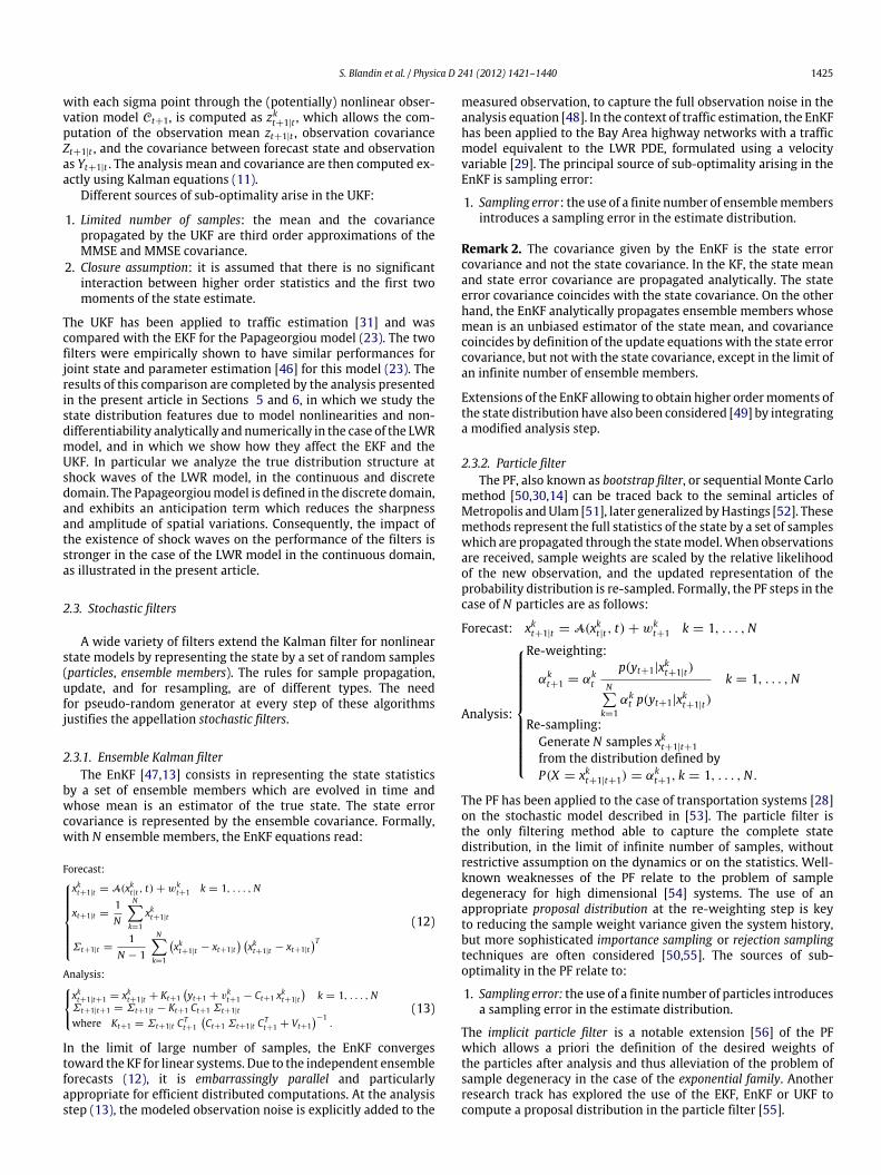
Fig. 3. Distribution of vehicle density at different space–time locations: Probability density function of the uncertainty ϱt,x on the true state (solid line), uniform probabilitydensity function with identical mean and variance (dotted line), probability density function ϱ̃t,x given by a deterministic shock-wave speed between the left and rightstochastic initial data (dashed line). This computation corresponds to a Greenshields fundamental diagram with uniform initial noise of variance 100. The true shock-waveis initially located at location 0 and does not move.
are neglected. The difference between the state distributionpropagated in this method and the true mixture distribution isillustrated in Fig. 3, for the same model parameters and initialcondition as in Fig. 2, with a variance 100 and 107 particles.Fig. 3 displays distributions corresponding to positive locations(0.01, 0.11, 0.21 miles), which corresponds to the right side of theleft sub-figure in Fig. 2. This is a situation in which P(ς > x
t ) <
P(ς < xt ) (more chance for the shock to be on the left than on
the right of location x at time t). This explains that the dominatingmode corresponds to the right initial data. The dominating modeis the only mode represented by the random field ϱ̃t,x, which isaccurate far from the shockwave only. The correlation representedby the non-uniform distribution of the dominating mode is notcaptured by the random field ϱ̃t,x. Additionally, we represent
a distribution3 with the same mean and variance as the truedistribution ϱt,x (which is the underlying principle of the UKF).This distribution (the dotted line) exhibits a large variance whichcaptures the variability due to the mixture nature of the truedistribution. One may note that this distribution includes negativevalues with non-zero probabilities, and positive values outsideof the admissible range according to the model, with non-zeroprobabilities.Remark 8. The solution to the stochastic Riemann problem givenby Eq. (29) may be accurate if the mixture from Eq. (28)
3 For graphical comparison, we use the same family as the initial condition, i.e. auniform distribution (represented in dotted line in Fig. 3).

S. Blandin et al. / Physica D 241 (2012) 1421–1440 1431
is degenerate and only one mode arises on each side of theshock wave. This is the case if the Rankine–Hugoniot speed isdeterministic, which may arise in the case of specific correlatedstatistics or if the solution to the Riemann problem is a contactdiscontinuity (e.g. in the case of piecewise linear fundamentaldiagrams, see Proposition 4).
Proposition 3. For a Greenshields fundamental diagram, if the leftinitial noise and the right initial noise are such that the sum ρl + ρris constant across all realizations ρl, ρr , then the random field ϱt,x isnot a mixture distribution.
Proof. The shock-wave speed associatedwith realizations ρl, ρr ofthe Riemann datum reads:
σG =
V ρl1 −
ρlρmax
− V ρr
1 −
ρrρmax
ρl − ρr
which can be rewritten as:
σG = V −Vρmax
(ρl + ρr)
which according to the assumption on the statistics is the same forall realizationsρl, ρr . The domainD is thus empty, and the randomfield ϱt,x is equal to the left or right datum. �
Proposition 4. For a triangular fundamental diagram, if Dl,Dr ⊆
[0, ρc] or Dl,Dr ⊆ [ρc, ρmax], the random field ϱt,x is not a mixture,for almost all (t, x) ∈ R+
\ {0} × R.
Proof. By assumption, we have ρl < ρr for all realizations of thetwo distributions. If Dl ⊆ [0, ρc] and Dr ⊆ [0, ρc], a realizationσT of the shock-wave speed ςT for the triangular diagram reads:
σT =Q (ρr)− Q (ρl)
ρr − ρl,
which can be rewritten using expression (16) and the fact thatρl ∈ Dl, ρr ∈ Dr , as:
σT =ρl V − ρr Vρl − ρr
= V
which yields a shock-wave speed equal to the free-flow speed forall realizations. Therefore the shock-wave speed is deterministic,and the random field solution of the Riemann problem is unimodalfor almost all (t, x) ∈ R+
\{0}×R. Similarly ifDl,Dr ⊆ [ρc, ρmax],the shock-wave speed is the speed of backward moving waves w.The domain D is thus empty, and the random field ϱt,x is equal tothe left or right datum. �
Consequently, for estimation using the CTM, when the traffic stateis completely in free-flow (Dl,Dr ⊆ [0, ρc]) or completely incongestion (Dl,Dr ⊆ [ρc, ρmax]), the estimate distributions onthe left and on the right do not mix and the normality assumptionof the initial condition estimates propagates (this conditionallinearity of the dynamics is used by the MKF).
5.2. Mixture solutions to the Godunov scheme
In this section, we analyze numerically how the emergenceof mixture distributions in the solution of the Riemann problemfor the stochastic datum relates to the emergence of mixturedistributions in the solution to the Godunov scheme. The Godunovscheme computes a numerical solution to the Cauchy problemon a discretization grid, by iteratively solving Riemann problemsbetween neighboring cells and averaging their solutions withineach cell. Numerical estimates produced in this manner differfrom the estimates obtained by solving the Riemann problem on
a continuous domain, due to numerical diffusion introduced in theaveraging step and the discrete setting. Additionally, in the intentof modeling numerical diffusion, discretization error and inherentmodeling error, it is common practice [2] to introduce an additiverandom source term to the discretized PDE (18). In order to studythe emergence ofmixture distributions in this context, we proposethe following numerical experiments.
We consider the Greenshields fundamental diagram with pa-rameters V = 80 mph, ρmax = 120 vpm, and the stochasticRiemann datum (ϱl = N (30, 100), ϱr = N (90, 100)) (we trun-cate the normal distribution to force its support into the admissibledomain [0, ρmax] of the model). Using Monte Carlo simulationswith 105 samples, we compute the (continuous) solution of theRiemann problem and the (discrete) solution of the Godunovschemewith Courant–Friedrichs–Lewy (CFL) [67] condition equal toone, spatially uniform left and right realizations of initial noise, andfor various discretization grid sizes and values of the model noise.
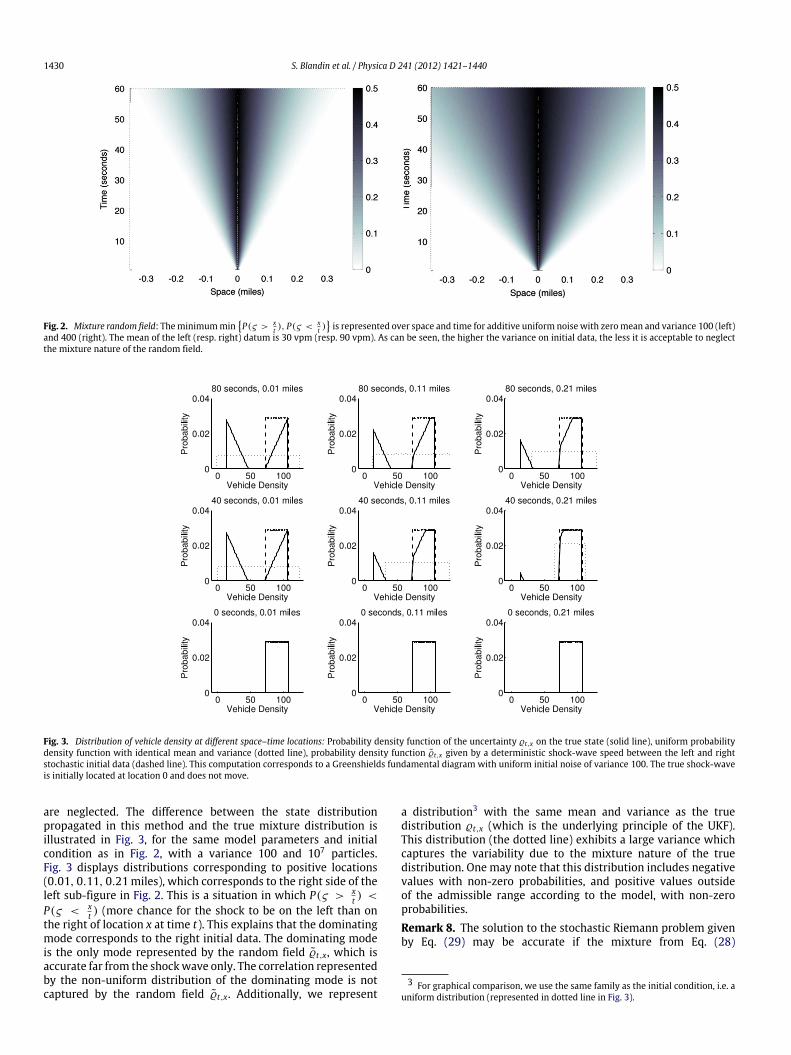
Numerical diffusion: The influence of numerical diffusion oncontinuous anddiscrete numerical estimates (see Fig. 4) is assessedby comparing the solution to the Riemann problem (solid line)with the solution to the Godunov scheme on a coarse grid (sixspace cells, 18 time-steps, dashed line) and on a fine grid (12space cells, 36 time-steps, dotted line). TheMonte Carlo simulationis run with 105 samples. As illustrated in Fig. 4, comparison ofthe numerical solutions on different grids illustrates that diffusionin the Godunov scheme smoothens the mixture nature of thesolution to the Riemann problem. The numerical solution exhibitstwo modes but due to diffusion, a non-zero probability arisesbetween the two modes. This illustrates that by discretizationof the constitutive model, the true nature of the distributionof uncertainty is blurred. This is not necessarily a problem ifthe discrete numerical model (Godunov scheme in this case)is considered to be the physical model, i.e. is considered torepresent the dynamics of the true state, as commonly donein transportation. However, it shows the limitation of discreteapproaches for estimation with continuous physical models, suchas the LWR PDE.
Model noise:We propose to compare (see Fig. 5) the continuoussolution to the Riemann problem (solid line), the discrete solutionto the Godunov scheme with no model noise (dotted line), andmodel noise represented by a random variable N (0, 50) (dashedline), on a grid with six space cells and 18 time-steps. The additionof amodel noise term to the Godunov scheme to account formodelerrors leads to a reduction of themixture nature of the distributionsolution to the stochastic Riemann problem. It induces a diffusionof the true distribution, which contributes to further smoothenthe two components of the mixture (see Fig. 5). This diffusion ismore structured that pure numerical diffusion (see Fig. 4), but thisexample clearly advocates for noise modeling in order to accountspecifically for discretization error as a function of the state and thecorresponding distribution of uncertainty [87–89].
Lack of correlation: The existence of mixture distributionsaround the discontinuity creates a correlation between the twosides of the shock wave (see Fig. 6). By propagating a singlecomponent of the mixture on each side of the shock wave, thecovariance structure is misrepresented by the linearized model.This is illustrated in Fig. 6 representing the covariance structureof the estimate at time-step 20, for a Monte Carlo simulationwith 104 particles in the left sub-figure, and for the linearizedmodel in the right sub-figure. The fundamental diagram is aGreenshields fundamental diagramwith parameters V = 80 mph,ρmax = 120 vpm, and the stochastic Riemann datum correspondsto (ϱl = N (15, 100), ϱr = N (75, 100)), in vehicles per mile. Thiscorresponds to a shock wave moving forward, starting at time 0from cell 0. One may note that due to the CFL condition, at time20, no physical correlation can exist farther than 20 cells around
1432 S. Blandin et al. / Physica D 241 (2012) 1421–1440
Fig. 4. Numerical diffusion: Themixture nature of the solution of the Riemann problem (solid line) is more accurately captured by the numerical solutionwith low numericaldiffusion (dotted line) computed on the fine grid than by the numerical solution with high numerical diffusion (dashed line) computed on the coarse grid.
Fig. 5. Model noise: the probability density function of the solution of the Riemann problem is represented by a solid line, the probability density function of the solution ofthe Godunov schemewith no noise is represented by a dotted line, the solution of the Godunov schemewith Gaussian centered model noise with variance 50 is representedby a dashed line.
the diagonal. The block diagonal structure of the linearized modelestimate at the shock wave appears clearly, whereas for theMonteCarlo simulation with 104 particles, the state error covariancematrix is band diagonal, which illustrates the correlation betweenthe two sides of the shock wave due to the mixture components.The comparison between the two figures displays the lack of
correlation, across the shock, of the covariance given by thelinearized model. In the absence of correlation, measurementsrealized on one side of the shock do not influence the estimateon the other side of the shock. The fact that the linearizedmodel overestimates the variance around cells neighboring thediscontinuity location is visible from the color scale.

S. Blandin et al. / Physica D 241 (2012) 1421–1440 1433
Fig. 6. State error log-covariance matrix: The shock wave is located at cell 10. The logarithm of the absolute value of the state error covariance matrix given by a Monte Carlosimulation with 104 particles (left) illustrates significant correlation between the two sides of the discontinuity, due to the existence of mixture distributions. The state errorcovariance given by a linearized model (right) is block-diagonal at the shock wave, due to the lack of correlation between the two sides of the shock wave in the linearizedmodel. This lack of correlation might be problematic for estimation, because measurements might not give information across shocks.
5.3. Discussion
In this section,we discuss how the properties of the distributionof the uncertainty on the true state solution of the Riemannproblem with stochastic datum relate to the accuracy of theestimate given by classical filters at the analysis step.
Forecast mean: The estimate given by the mean of thedistribution obtained by deterministic propagation of the meanof the left and right data (case of EKF), with additive modelnoise, seems biased since it only captures one component of themixture (see Fig. 3 as well for instance). Close to the shock wave,the diffusivity of the Godunov scheme numerically alleviates thisdrawback by smoothing the mixture through diffusion. The bias atthe shock wave due to mixture uncertainty is less likely to occurwith sample-based filters which implicitly consider a stochasticmodel through the propagation of samples by a deterministicmodel (see experiments below). We reemphasize here that thetrue shock-wave speed for Figs. 3 and 4 is zero, hence the trueshock wave does not move from location 0.
Forecast variance: As illustrated in Fig. 3, close to the shockwave, even when the mean and the variance of the uncertainty onthe true state are propagated accurately, representing the mixturedistribution of the uncertainty by a unimodal distribution leadsto considering a variance corresponding to the two modes, hencea greater dependency on the observations at the analysis step,through an increased gain, which is due to a poor representationof the uncertainty related to the prior distribution. On the otherhand, if only a singlemode of the uncertainty is accurately captured(case of EKF), the estimate exhibits a lower variance than theuncertainty, which is a classical cause of divergence of the filter.
Analysis step with mixture uncertainty: We consider the caseof a stationary shock wave with left and right initial data(ϱl = N (30, 100), ϱr = N (90, 100)), for a Greenshields funda-mental diagram with parameters V = 80 mph, ρmax = 120 vpm.The true stationary shockwave is located at location 20.5 through-out each simulation. Figs. 7 and 8 display the prior and posteriortrue uncertainty, and respectively the normal distributions corre-sponding to the EKF estimate and the EnKF ensemble estimates4, aswell as the observations. The prior distribution of the uncertaintyon the true state is computed by Monte Carlo simulation with 105
particles, and its posterior obtained by full Bayesian update. Westudy the characteristics of the analysis step of the EKF and theEnKF, at different times,with a single observationwith observation
4 Even though the EnKF propagates and updates ensemble, for visual consistencyin a context of minimum variance estimation, and due to the low number ofensemble members used, we present the normal distribution corresponding to theensemble members distribution.
noise variance 100. The posterior computed by the analysis is notpropagated further but simply displayed. Thismeans that each rowin Figs. 7 and 8 corresponds to a different value of the true state, adifferent realization of the observation noise, and a single analysisstep. For the sake of comparison we always sample an observationat location 21.
The sensitivity of the filters to the observation is illustratedby the significant difference between the prior and the posterior(respectively dotted and dashed lines), around the shock wave,for both the EKF and the EnKF. At the location of the observation(location 21), the prior provided by the EKF, which only capturesa single mode, is more inaccurate than the prior given bythe EnKF, which can account partially for mixture distributionsrepresentation with ensemble members. However, after analysis,the posteriors for the two filters are very similar at the locationof the observation. Away from the shock wave (location 19 and22), it is clear that the EKF estimate exhibits a non-consistent errorvariance (simulations 1, 2, 3 in particular).
The correlation across the shock wave clearly discriminates thetwo filters. Across the shock wave, at location 20, the posteriorgiven by the EKF (dashed line) is often centered on the wrongmode of the posterior uncertainty (dash–dotted line). This is notthe case for the EnKFwhich captures the twomodes of themixturein most cases. When the observation corresponds to a mode ofthe mixture uncertainty not well represented by the estimate (forinstance run 2, location 21 of Fig. 7), it can be noted that theposterior distribution can provide more inaccurate estimate thanthe prior; for instance the posterior given by the EKF (dashed line)for run 2, location 20, is outside the range of values represented.This illustrates the difficulty of capturing true correlation inducedby mixture uncertainty across the shock wave.
The mixture nature of the uncertainty is clearly reducedby the observation, however, the two modes are still presentand propagate in the posterior uncertainty (dash–dotted line atlocation 19 and 20 for simulation 1, location 22 for simulation 2,location 20 for simulation 3).
These numerical examples illustrate the limitations of thesuboptimal MMSE estimates provided by the EKF and EnKF, inthe case of mixture distributions arising in traffic flow aroundshock waves. Stochastic filters such as the EnKF are more robustto the mixture nature of the uncertainty, since their samplerepresentation allows them to better capture the full varianceof the two modes of the distribution of the uncertainty on thetrue state. However, this leads to higher sensitivity of the filterand may lead to instabilities at shock waves. On the other hand,deterministic filters able to capture only a single mode of thedistribution of the uncertainty on the true state exhibit a lowervariance than the uncertainty, which may cause divergence of theestimate if the models have low error terms.

1434 S. Blandin et al. / Physica D 241 (2012) 1421–1440
Fig. 7. EKF analysis step: the analysis step at different times is represented for a stationary shock wave at location 20.5, between 30 and 90 vpm, initial condition noisevariance 100, and observation noise variance 100. The observation is represented by a circular marker. The prior distribution of the uncertainty on the true state obtainedby Monte Carlo simulation with 105 samples is represented by a solid line, the posterior distribution obtained by Bayesian update is represented by a dash–dotted line. Theprior distribution given by propagation through the linearized model is represented by a dotted line, and the posterior distribution given by the analysis step of the EKF isrepresented by a dashed line.
6. Model non-differentiability
In this section, we show that the numerical Godunov flux de-fined in (18)–(19) is non-differentiable. We prove that conse-quently, the discrete-time dynamics of the Godunov scheme isnon-differentiable, which prevents straightforward application offiltering algorithms requiring differentiability to discrete trans-portation models based on the Godunov scheme.
6.1. Characterization of non-differentiability domain
The Godunov scheme consists of a dynamical system (18)resulting from the discretization of the transport equation (14)where the numerical flux qG(·, ·) can be defined in a piecewisemanner on regular sub-domains in the case of a concave flux with
a single maximum (19). The following proposition states the lackof continuous differentiability at a specific boundary between twoof these sub-domains.
Proposition 5. On the domain S defined as:
S =(ρl, ρr) ∈ [0, ρmax]2 | ρl < ρr and Q (ρl) = Q (ρr)
, (30)
the numerical Godunov flux (19) is not differentiable.
Proof. The expression of the numerical Godunov flux is given byEq. (19). In each sub-domain of definition corresponding to eachline of (19), if the flux function Q (·) is differentiable, the numericalflux qG(·, ·) is also left and right differentiable. It is straightforwardto compute its left and right derivative on each sub-domain:

S. Blandin et al. / Physica D 241 (2012) 1421–1440 1435
Fig. 8. EnKF analysis step: the analysis step at different times is represented for a stationary shock wave at location 20.5, between 30 and 90 vpm, initial condition noisevariance 100, and observation noise variance 100. The observation represented by a circular marker. The prior distribution of the uncertainty on the true state obtained byMonte Carlo simulation with 105 samples is represented by a solid line, the posterior distribution obtained by Bayesian update is represented by a dash–dotted line. Theestimate distributions given by the EnKF are represented as normal distributions with corresponding mean and variance. The prior given by propagation of 40 ensemblemembers is represented as a normal distribution by a dotted line, and the posterior given by the analysis step of the EnKF is represented as a normal distribution by a dashedline.
∂qG∂ρl
(ρl, ρr)
=
Q ′(ρl) if ρr ≤ ρl < ρc0 if ρr ≤ ρc ≤ ρl0 if ρc < ρr ≤ ρlQ ′(ρl) if Q (ρl) < Q (ρr)0 if Q (ρl) > Q (ρr)
if ρl < ρr
(31)
∂qG∂ρr
(ρl, ρr)
=
0 if ρr ≤ ρl < ρc0 if ρr ≤ ρc ≤ ρlQ ′(ρr) if ρc < ρr ≤ ρl0 if Q (ρl) < Q (ρr)Q ′(ρr) if Q (ρl) > Q (ρr)
if ρl < ρr .
(32)
As indicated by the fourth case of Eq. (31) (or equivalently for theright derivative with the fourth case of Eq. (32)), the left derivativeof the numerical flux is only defined on the left and on the right
of the domain S defined by Eq. (30), with the left value beingQ ′(ρl) and the right value being 0. The left and right values areequal only at the capacity point (point of maximal flux), in the caseof a flux differentiable at capacity. Since the left derivative is notdifferentiable on S, the numerical flux is not differentiable on itsdomain of definition. �
The domain of non-differentiability of the numerical Godunovscheme corresponds to the locus of stationary shock waves.In particular, the numerical Godunov flux and the discretedynamics associated with the Godunov scheme are differentiableat moving shock waves. In the case of discretization schemeswith higher numerical viscosity, for instance the Lax–Friedrichsnumerical scheme [67], differentiability is obtained everywherebut numerical approximation of discontinuities is less accurate.
Proposition 6. The discrete time dynamics of the Godunov schemeis non-differentiable, and in the case of a differentiable flux functionQ (·), the non-differentiability domain consists of the locus S ofstationary shock waves.

1436 S. Blandin et al. / Physica D 241 (2012) 1421–1440
Fig. 9. Locus of non-differentiability of the numerical Godunov flux: The top, middle and bottom rows respectively correspond to the Greenshields, triangular, and exponentialfundamental diagrams. The Godunov flux is defined in a piecewisemanner on the three sub-domains delimited by solid or dashed lines. A dashed line indicates discontinuityacross the boundary of the domain, whereas a solid line indicates continuity at the boundary. The three diagrams exhibit non-differentiability of the locus of stationary shockwaves (center and right column, oblique curve). Additionally, the triangular diagram (middle row) exhibits non-differentiability at the critical density.
Proof. The numerical flux is non-differentiable in the domain Sdefined by (30). Since it is impossible to have at the same time(ρn
i−1, ρni ) ∈ S and (ρn
i , ρni+1) ∈ S, the discrete time dynamics
defined by (18) is non-differentiable. In the case of a differentiableflux function Q (·), the numerical flux is also differentiable in allits sub-domains of definition, and it can be checked in Fig. 9 thatit is also continuously differentiable at their boundaries, thus Sis the non-differentiability domain of the discrete time dynamicsassociated with the Godunov scheme. �
The non-differentiability of the discrete dynamics associatedwith the Godunov scheme does not result from a numerical issuebut results from the structure of the solution of the continuouspartial differential equation considered. This can be verified byconsidering the solution to the Riemann problem in the case of astationary shock wave. The solution that consists of upstream anddownstream densities with equal fluxes is stationary. However, itis clear that a slight perturbation of the upstream or downstreamdensity causes the shock wave to propagate and the domaincorresponding to the left or right initial condition to eventuallyprevail, depending on the flux balance at the discontinuity.
Remark 9. In the case of non-differentiable flux functions Q (·)such as the triangular flux function or the Smulders flux function,it is clear that the dynamics of the numerical solution is notdifferentiable. However, since the flux function results from
an empirical fit, the flux function can be approximated by asmooth function with relatively small consequences. The non-differentiability described in Proposition 5 results from theintrinsic properties of the conservation law, which can only befixed by modifying the constitutive physical principles of themodel.
Remark 10. For junction problems modeled as the maximizationof a linear objective function of the traffic state under linearinequality constraints (see Remark 3), the optimum is alwaysattained at a vertex of the constraint polytopes, hence the flowthrough the junction is not a differentiable function of the trafficstate and the same difficulties happen there as well.
6.2. Numerical experiments
In this section, we analyze the estimation error induced by thelack of differentiability of the numerical Godunov flux at the locusof stationary shock waves.
For clarity we present results for the case of the Greenshieldsflux function (15) (with parameters V = 80 mph and ρmax = 120vpm, as in the previous section), which is differentiable on itsdomain of definition. Similarly, in order to simplify the analysis,we consider only initial condition noise, drawn from i.i.d. normaldistribution N (0, 100). The model noise is considered to be 0. Weuse the Godunov scheme (18), with CFL condition [67] equal to 1,

S. Blandin et al. / Physica D 241 (2012) 1421–1440 1437
Fig. 10. Mean error growth: the growth with time of the relative L2 error on the mean is represented for a linearized model (left) and a Monte Carlo simulation with 50particles (right). The solid line corresponds to the case of a stationary shock wave with ρl = 30 vpm, ρr = 90 vpm, the dashed line corresponds to the case of a movingshock wave, with ρl = 15 vpm, ρr = 75 vpm, the dotted lined corresponds to the case of a rarefaction wave, with ρl = 90 vpm, ρr = 30 vpm.
Fig. 11. Covariance error growth: the growth with time of the relative error on the error covariance trace is represented for a linearized model (left) and a Monte Carlosimulation with 50 particles (right). The solid line corresponds to the case of a stationary shock wave with ρl = 30 vpm, ρr = 90 vpm, the dashed line corresponds to thecase of a moving shock wave, with ρl = 15 vpm, ρr = 75 vpm, the dotted lined corresponds to the case of a rarefaction wave, with ρl = 90 vpm, ρr = 30 vpm.
and 80 cells in space. The distribution of the uncertainty on thetrue state is computed using a Monte Carlo simulation with 104
particles, and the forecast moments using different propagationmodels are compared against the true moments. In order to assessthe accuracy of the estimate covariance, we compute two errormetrics. The error metric for the mean, in Fig. 10, is the relativeL2 error:∥µe − µ∥2
∥µ∥2
where µe denotes the estimated mean using the forecast stepof a model, and µ is the true forecast. The error metric for thecovariance, in Fig. 11, is the relative absolute error on the errorcovariance trace, defined by:
trace(|Σ̃ −Σ |)
trace(Σ)
where Σ̃ denotes the estimated error covariance given by theforecast model andΣ denotes the true error covariance.
Estimate error: The error induced by the use of a linearizationmethod at the locus of the stationary shock wave is illustrated bya solid line in Fig. 10 for the mean and in Fig. 11 for the covariance,for the use of the derivative of the numerical Godunov flux on theleft at its point of non-differentiability. For state propagation usinga Monte Carlo method with 50 particles (right sub-figure) or thelinearized model (right sub-figure), the shock waves lead to thehighest error, which is due to the fact that only entropic shockwaves are propagated by the scheme; the uncertainty associatedwith the initial condition propagates toward the shock-wavelocation. In the case of a rarefaction, the uncertainty associatedwith the initial datum propagates outward, and the centered fanis deterministic.
The state error covariance given by forward simulation usingthe linearized dynamics diverges in time from the covariance ofthe uncertainty on the true state (see Fig. 11 left). In the case of astationary shock wave (solid line), the divergence is slightly fasterthan in the case of a moving shock wave. In particular, noting thatthe oscillations in the curve associated with a moving shock wave(dashed line) in Fig. 10 and Fig. 11 correspond to a change of cellsand that the meaningful error for this phenomenon correspondsto the lower envelope of this curve, the divergence associatedwith the stationary shockwave is noticeably greater. However, onemay note that Fig. 10, left, and Fig. 11, left, only correspond toconsidering the derivative on the left at the non-differentiabilitylocus. Different weightings of the left and right derivative at thenon-differentiability domain might lead to better results.
6.3. Discussion
In this section we analyze the consequences of non-differenti-ability of the dynamics of theGodunov scheme for state estimation.
As illustrated in Fig. 10 left, the trend of the estimation errordue to model nonlinearity is comparable for the stationary shockwave (solid line) and for the moving shock wave (dashed line).This is consistent with the fact that the propagation of the estimatemean in the linearizedmodel does not involve differentiability. Theerror introduced is simply due to the nonlinearity of shock waveswith the Greenshields flux function. In the case of the rarefactionwave (dotted line), the estimation error is much smaller due tothe entropy condition and the fact that information propagatesoutward from the initial discontinuity.
For a moving shock wave (dashed line), the error exhibits atypical oscillation feature due to error of location of the shockwave. The increasing part of the oscillation corresponds to the

1438 S. Blandin et al. / Physica D 241 (2012) 1421–1440
Fig. 12. Posterior mean error: the mean L2 error of the posterior for 103 draws of the observation at each location, is represented as a function of the observation location foran analysis with prior covariance obtained by Monte Carlo simulation with 104 samples (solid line), and for an analysis with prior covariance propagated by the linearizedmodel (dashed line). Top, middle, and bottom row respectively correspond to observation noise standard deviation of 10, 32, and 100. The prior shock wave, represented asa vertical dotted line, is located between cells 6 and 7 for all simulations. For the left, middle, and right columns, the true shock wave, represented as a vertical dashed line,is respectively located between cells 6 and 7, 3 and 4, and 0 and 1.
mixture nature of the distribution of the uncertainty arising in thecell where the shock wave will move, hence increasing the errorwith the linearized model. The decreasing part of the oscillationcorresponds to the shock wave actually propagating to the cell,and reducing the error. The finite slope on the decreasing partcorresponds to the effect of diffusion.
The non-differentiability of the numerical flux introduces anerror in the error covariance which increases with time at arate noticeably greater than the error growth rate in the errorcovariance for a moving shock wave (see Fig. 11 left in which thetrend of the solid line is comparable to the trend of the top of thepeaks of the dashed line).
Inaccurate estimation of the state covariance at the forecaststep, depicted in Fig. 11, impacts the use of measurements at theanalysis step. This is illustrated in Fig. 12, in which we consideran analysis done at time 40, for the case of the stationary shockwave, with the same parameters used in Fig. 11. We compare theposterior error covariance computed by the analysis step definedby the Kalman filter (5), with on one hand a covariance computedby propagation of the initial condition covariance through thelinearized state model, and on the other hand a covariancecomputed by aMonte Carlo simulationwith 104 samples. The priormeans and the observations are identical for both cases, hence thediscrepancy in the posteriors is solely due to the discrepancy in theprior covariances and results from the inaccuracy of the covariancepropagated by the linearized non-differentiable model. A MonteCarlo simulation with 104 samples is considered to provide thedistribution of the uncertainty on the true state.
As illustrated in Fig. 12, the error associated with the priorcovariance induces an error in the posterior mean. In particular,for observations close to the discontinuity, one can note that the
error in the posterior can be higher than the prior error, whichcorresponds to the horizontal line. The inability to capture thecovariance structure at the shock wave, presented in the previoussection, is also visible in the case of an accurate prior (left column)with a different posterior error for observations located on theleft or on the right of the shock wave, although the problemis symmetric, as illustrated by the posterior error for the truecovariance error in that case.
The fact that the filter may diverge due to the wrong covariancestructure propagation by the linearizednon-differentiablemodel isillustrated in Fig. 13 in which we present the posterior covariancefor the two different analyses described above, on one handwith the covariance propagated by the linearized model, andon the other hand with the covariance associated with thetrue distribution of uncertainty, computed using a Monte Carlosimulation with 105 samples and the parameters of Fig. 12 leftcolumn.
For observation with low error located close to the shock-wavelocation, the analysis can cause the linearized filter to divergeby introducing a covariance lower than the covariance on theuncertainty. This echoes the analysis on the nonlinearity and thedifficulty to model correctly the correlation structure at shockwaves. In particular it is clear that observations away from shockwaves do not particularly improve the estimates, and observationsclose to shock waves can potentially decrease the accuracy of theestimates and performance of the filter at the next time step.
7. Conclusion
In this article, we showed that the classical scalar macroscopictraffic models based on the Lighthill–Whitham–Richards partial
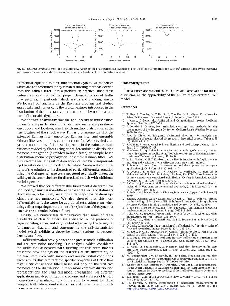
S. Blandin et al. / Physica D 241 (2012) 1421–1440 1439
Fig. 13. Posterior covariance error: the posterior covariance for the linearized model (dashed) and for the Monte Carlo simulation with 105 samples (solid) with respectiveprior covariance as circle and cross, are represented as a function of the observation location.
differential equation exhibit fundamental dynamical propertieswhich are not accounted for by classical filtering methods derivedfrom the Kalman filter. It is a problem in practice, since thesefeatures are essential for the proper characterization of trafficflow patterns, in particular shock waves and standing waves.We focused our analysis on the Riemann problem and studiedanalytically and numerically the typical features introduced in thedistribution of the uncertainty on the true state by nonlinear andnon-differentiable dynamics.
We showed analytically that the nonlinearity of traffic causesthe uncertainty in the state to translate into uncertainty in shock-wave speed and location, which yields mixture distribution at thetrue location of the shock wave. This is a phenomenon that theextended Kalman filter, unscented Kalman filter and ensembleKalman filter assumptions do not account for. We provided ana-lytical computations of the resulting errors in the estimate distri-butions provided by filters using either deterministic distributionmoment propagation (extended Kalman filter) or sample-baseddistribution moment propagation (ensemble Kalman filter). Wediscussed the resulting estimation errors caused by misrepresent-ing the estimate as a unimodal distribution. Numerical computa-tions of the solution to the discretized partial differential equationusing the Godunov scheme were proposed to critically assess thevalidity of these conclusions for discretizedmodelswith additionalmodeling error.
We proved that for differentiable fundamental diagrams, theGodunov dynamics is non-differentiable at the locus of stationaryshock waves, which may arise for all density–flow relationshipswhich are not monotonic. We also showed that this non-differentiability is the cause for additional estimation error whenusing a filter requiring computation of the Jacobian of the dynamics(such as the extended Kalman filter).
Finally, we numerically demonstrated that some of thesedrawbacks of classical filters are alleviated in the presence oflarge modeling errors and very limited when using the triangularfundamental diagram, and consequently the cell-transmissionmodel, which exhibits a piecewise linear relationship betweendensity and flow.
Traffic estimationheavily depends onprecisemodel calibration,and accurate noise modeling. Our analysis, which consideredthe difficulties associated with filtering for true state models,presented new findings on the statistics of the uncertainty onthe true state even with smooth and normal initial conditions.These results illustrate that the specific properties of traffic flowmay justify considering filters based not only on the first twomoments of the distribution, but on more complex distributionrepresentations, and using full model propagation. For differentapplications and depending on the volume and accuracy of trustedmeasurements available, new filters able to account for thesecomplex traffic-dependent statistics may allow us to significantlyincrease estimate accuracy.
Acknowledgments
The authors are grateful to Dr. Olli-Pekka Tossavainen for initialdiscussion on the applicability of the EKF to the discretized LWRmodel.
References
[1] T. Hey, S. Tansley, K. Tolle (Eds.), The Fourth Paradigm: Data-IntensiveScientific Discovery, Microsoft Research, Redmond, WA, 2009.
[2] J. Kaipio, E. Somersalo, Statistical and Computational Inverse Problems,Springer, New-York, NY, 2005.
[3] F. Bouttier, P. Courtier, Data assimilation concepts and methods, Trainingcourse notes of the European Centre for Medium-Range Weather Forecasts,1999, Reading, UK.
[4] F.-X. Le Dimet, O. Talagrand, Variational algorithms for analysis andassimilation of meteorological observations: theoretical aspects, Tellus A 38(2) (1986) 97–110.
[5] R. Kalman, A new approach to linear filtering and prediction problems, J. BasicEng. 82 (1) (1960) 35–45.
[6] N. Wiener, Extrapolation, interpolation, and smoothing of stationary time se-rieswith engineering applications, The Technology Press of TheMassachusettsInstitute of Technology, Boston, MA, 1949.
[7] Y. Bar-Shalom, X. Li, T. Kirubarajan, J. Wiley, Estimation with Applications toTracking and Navigation, John Wiley and Sons, New York, NY, 2001.
[8] S. Schmidt, Kalman filter: Its recognition and development for aerospaceapplications, J. Guid. Control 4 (1) (1981) 4–7.
[9] P. Courtier, E. Andersson, W. Heckley, D. Vasiljevic, M. Hamrud, A.Hollingsworth, F. Rabier, M. Fisher, J. Pailleux, The ECMWF implementationof three-dimensional variational assimilation (3D-Var). I: Formulation, Q. J. R.Meteorol. Soc. 124 (550) (1998) 1783–1807.
[10] P. Courtier, J. Thepaut, A. Hollingsworth, A strategy for operational implemen-tation of 4D-Var, using an incremental approach, Q. J. R. Meteorol. Soc. 120(519) (1994) 1367–1387.
[11] B. Anderson, J. Moore, Optimal Filtering, Prentice Hall, Upper Saddle River, NJ,1979.
[12] S. Julier, J. Uhlmann, A newextension of the Kalman filter to nonlinear systems,in: Proceedings of AeroSense: SPIE 11th Annual International Symposium onAerospace/Defense Sensing, Simulation and Controls, Orlando, FL, 1997.
[13] G. Evensen, The ensemble Kalman filter: Theoretical formulation and practicalimplementation, Ocean Dynam. 53 (4) (2003) 343–367.
[14] J. Liu, R. Chen, Sequential Monte Carlo methods for dynamic systems, J. Amer.Statist. Assoc. 93 (443) (1998) 1032–1044.
[15] R. Chen, J. Liu, Mixture Kalman filters, J. R. Stat. Soc. Ser. B (Stat. Methodol.) 62(3) (2000) 493–508.
[16] D. Gazis, C. Knapp, On-line estimation of traffic densities from time-series offlow and speed data, Transp. Sci. 5 (3) (1971) 283–301.
[17] M. Szeto, D. Gazis, Application of Kalman filtering to the surveillance andcontrol of traffic systems, Transp. Sci. 6 (4) (1972) 419–439.
[18] Y. Wang, M. Papageorgiou, Real-time freeway traffic state estimation basedon extended Kalman filter: a general approach, Transp. Res. 39 (2) (2005)141–167.
[19] Y. Wang, M. Papageorgiou, A. Messmer, Real-time freeway traffic stateestimation based on extended Kalman filter: A case study, Transp. Sci. 41 (2)(2007) 167.
[20] M. Papageorgiou, J.-M. Blosseville, H. Hadj-Salem, Modelling and real-timecontrol of traffic flow on the southern part of Boulevard Peripherique in Paris:Part I: Modelling, Transp. Res. 24 (5) (1990) 345–359.
[21] T. Schreiter, C. van Hinsbergen, F. Zuurbier, H. van Lint, S. Hoogendoorn, Data-model synchronization in extended Kalman filters for accurate online trafficstate estimation, in: 2010 Proceedings of the Traffic Flow Theory Conference,Annecy, France, 2010.
[22] S. Smulders, Control of freeway traffic flow by variable speed signs, Transp.Res. 24 (2) (1990) 111–132.
[23] J.-C. Herrera, A. Bayen, Incorporation of lagrangian measurements infreeway traffic state estimation, Transp. Res. 44 (4) (2010) 460–481.http://dx.doi.org/10.1016/j.trb.2009.10.005.
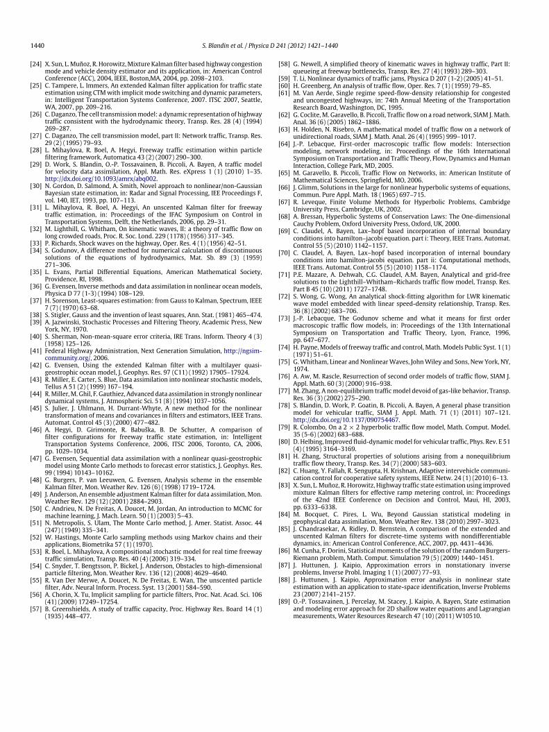
1440 S. Blandin et al. / Physica D 241 (2012) 1421–1440
[24] X. Sun, L.Muñoz, R. Horowitz,MixtureKalman filter basedhighway congestionmode and vehicle density estimator and its application, in: American ControlConference (ACC), 2004, IEEE, Boston,MA, 2004, pp. 2098–2103.
[25] C. Tampere, L. Immers, An extended Kalman filter application for traffic stateestimation using CTMwith implicit mode switching and dynamic parameters,in: Intelligent Transportation Systems Conference, 2007. ITSC 2007, Seattle,WA, 2007, pp. 209–216.
[26] C. Daganzo, The cell transmissionmodel: a dynamic representation of highwaytraffic consistent with the hydrodynamic theory, Transp. Res. 28 (4) (1994)269–287.
[27] C. Daganzo, The cell transmission model, part II: Network traffic, Transp. Res.29 (2) (1995) 79–93.
[28] L. Mihaylova, R. Boel, A. Hegyi, Freeway traffic estimation within particlefiltering framework, Automatica 43 (2) (2007) 290–300.
[29] D. Work, S. Blandin, O.-P. Tossavainen, B. Piccoli, A. Bayen, A traffic modelfor velocity data assimilation, Appl. Math. Res. eXpress 1 (1) (2010) 1–35.http://dx.doi.org/10.1093/amrx/abq002.
[30] N. Gordon, D. Salmond, A. Smith, Novel approach to nonlinear/non-GaussianBayesian state estimation, in: Radar and Signal Processing, IEE Proceedings F,vol. 140, IET, 1993, pp. 107–113.
[31] L. Mihaylova, R. Boel, A. Hegyi, An unscented Kalman filter for freewaytraffic estimation, in: Proceedings of the IFAC Symposium on Control inTransportation Systems, Delft, the Netherlands, 2006, pp. 29–31.
[32] M. Lighthill, G. Whitham, On kinematic waves, II: a theory of traffic flow onlong crowded roads, Proc. R. Soc. Lond. 229 (1178) (1956) 317–345.
[33] P. Richards, Shock waves on the highway, Oper. Res. 4 (1) (1956) 42–51.[34] S. Godunov, A difference method for numerical calculation of discontinuous
solutions of the equations of hydrodynamics, Mat. Sb. 89 (3) (1959)271–306.
[35] L. Evans, Partial Differential Equations, American Mathematical Society,Providence, RI, 1998.
[36] G. Evensen, Inversemethods and data assimilation in nonlinear oceanmodels,Physica D 77 (1-3) (1994) 108–129.
[37] H. Sorenson, Least-squares estimation: from Gauss to Kalman, Spectrum, IEEE7 (7) (1970) 63–68.
[38] S. Stigler, Gauss and the invention of least squares, Ann. Stat. (1981) 465–474.[39] A. Jazwinski, Stochastic Processes and Filtering Theory, Academic Press, New
York, NY, 1970.[40] S. Sherman, Non-mean-square error criteria, IRE Trans. Inform. Theory 4 (3)
(1958) 125–126.[41] Federal Highway Administration, Next Generation Simulation, http://ngsim-
community.org/, 2006.[42] G. Evensen, Using the extended Kalman filter with a multilayer quasi-
geostrophic ocean model, J. Geophys. Res. 97 (C11) (1992) 17905–17924.[43] R. Miller, E. Carter, S. Blue, Data assimilation into nonlinear stochastic models,
Tellus A 51 (2) (1999) 167–194.[44] R.Miller,M. Ghil, F. Gauthiez, Advanced data assimilation in strongly nonlinear
dynamical systems, J. Atmospheric Sci. 51 (8) (1994) 1037–1056.[45] S. Julier, J. Uhlmann, H. Durrant-Whyte, A new method for the nonlinear
transformation of means and covariances in filters and estimators, IEEE Trans.Automat. Control 45 (3) (2000) 477–482.
[46] A. Hegyi, D. Girimonte, R. Babuška, B. De Schutter, A comparison offilter configurations for freeway traffic state estimation, in: IntelligentTransportation Systems Conference, 2006, ITSC 2006, Toronto, CA, 2006,pp. 1029–1034.
[47] G. Evensen, Sequential data assimilation with a nonlinear quasi-geostrophicmodel using Monte Carlo methods to forecast error statistics, J. Geophys. Res.99 (1994) 10143–10162.
[48] G. Burgers, P. van Leeuwen, G. Evensen, Analysis scheme in the ensembleKalman filter, Mon. Weather Rev. 126 (6) (1998) 1719–1724.
[49] J. Anderson, An ensemble adjustment Kalman filter for data assimilation, Mon.Weather Rev. 129 (12) (2001) 2884–2903.
[50] C. Andrieu, N. De Freitas, A. Doucet, M. Jordan, An introduction to MCMC formachine learning, J. Mach. Learn. 50 (1) (2003) 5–43.
[51] N. Metropolis, S. Ulam, The Monte Carlo method, J. Amer. Statist. Assoc. 44(247) (1949) 335–341.
[52] W. Hastings, Monte Carlo sampling methods using Markov chains and theirapplications, Biometrika 57 (1) (1970).
[53] R. Boel, L. Mihaylova, A compositional stochastic model for real time freewaytraffic simulation, Transp. Res. 40 (4) (2006) 319–334.
[54] C. Snyder, T. Bengtsson, P. Bickel, J. Anderson, Obstacles to high-dimensionalparticle filtering, Mon. Weather Rev. 136 (12) (2008) 4629–4640.
[55] R. Van Der Merwe, A. Doucet, N. De Freitas, E. Wan, The unscented particlefilter, Adv. Neural Inform. Process. Syst. 13 (2001) 584–590.
[56] A. Chorin, X. Tu, Implicit sampling for particle filters, Proc. Nat. Acad. Sci. 106(41) (2009) 17249–17254.
[57] B. Greenshields, A study of traffic capacity, Proc. Highway Res. Board 14 (1)(1935) 448–477.
[58] G. Newell, A simplified theory of kinematic waves in highway traffic, Part II:queueing at freeway bottlenecks, Transp. Res. 27 (4) (1993) 289–303.
[59] T. Li, Nonlinear dynamics of traffic jams, Physica D 207 (1-2) (2005) 41–51.[60] H. Greenberg, An analysis of traffic flow, Oper. Res. 7 (1) (1959) 79–85.[61] M. Van Aerde, Single regime speed-flow-density relationship for congested
and uncongested highways, in: 74th Annual Meeting of the TransportationResearch Board, Washington, DC, 1995.
[62] G. Coclite, M. Garavello, B. Piccoli, Traffic flow on a road network, SIAM J.Math.Anal. 36 (6) (2005) 1862–1886.
[63] H. Holden, N. Risebro, A mathematical model of traffic flow on a network ofunidirectional roads, SIAM J. Math. Anal. 26 (4) (1995) 999–1017.
[64] J.-P. Lebacque, First-order macroscopic traffic flow models: Intersectionmodeling, network modeling, in: Proceedings of the 16th InternationalSymposium on Transportation and Traffic Theory, Flow, Dynamics andHumanInteraction, College Park, MD, 2005.
[65] M. Garavello, B. Piccoli, Traffic Flow on Networks, in: American Institute ofMathematical Sciences, Springfield, MO, 2006.
[66] J. Glimm, Solutions in the large for nonlinear hyperbolic systems of equations,Commun. Pure Appl. Math. 18 (1965) 697–715.
[67] R. Leveque, Finite Volume Methods for Hyperbolic Problems, CambridgeUniversity Press, Cambridge, UK, 2002.
[68] A. Bressan, Hyperbolic Systems of Conservation Laws: The One-dimensionalCauchy Problem, Oxford University Press, Oxford, UK, 2000.
[69] C. Claudel, A. Bayen, Lax–hopf based incorporation of internal boundaryconditions into hamilton–jacobi equation. part i: Theory, IEEE Trans. Automat.Control 55 (5) (2010) 1142–1157.
[70] C. Claudel, A. Bayen, Lax–hopf based incorporation of internal boundaryconditions into hamilton-jacobi equation. part ii: Computational methods,IEEE Trans. Automat. Control 55 (5) (2010) 1158–1174.
[71] P.E. Mazare, A. Dehwah, C.G. Claudel, A.M. Bayen, Analytical and grid-freesolutions to the Lighthill–Whitham–Richards traffic flow model, Transp. Res.Part B 45 (10) (2011) 1727–1748.
[72] S. Wong, G. Wong, An analytical shock-fitting algorithm for LWR kinematicwave model embedded with linear speed-density relationship, Transp. Res.36 (8) (2002) 683–706.
[73] J.-P. Lebacque, The Godunov scheme and what it means for first ordermacroscopic traffic flow models, in: Proceedings of the 13th InternationalSymposium on Transportation and Traffic Theory, Lyon, France, 1996,pp. 647–677.
[74] H. Payne, Models of freeway traffic and control, Math. Models Public Syst. 1 (1)(1971) 51–61.
[75] G.Whitham, Linear and NonlinearWaves, JohnWiley and Sons, New York, NY,1974.
[76] A. Aw, M. Rascle, Resurrection of second order models of traffic flow, SIAM J.Appl. Math. 60 (3) (2000) 916–938.
[77] M. Zhang, A non-equilibrium trafficmodel devoid of gas-like behavior, Transp.Res. 36 (3) (2002) 275–290.
[78] S. Blandin, D. Work, P. Goatin, B. Piccoli, A. Bayen, A general phase transitionmodel for vehicular traffic, SIAM J. Appl. Math. 71 (1) (2011) 107–121.http://dx.doi.org/10.1137/090754467.
[79] R. Colombo, On a 2 × 2 hyperbolic traffic flow model, Math. Comput. Model.35 (5-6) (2002) 683–688.
[80] D. Helbing, Improved fluid-dynamicmodel for vehicular traffic, Phys. Rev. E 51(4) (1995) 3164–3169.
[81] H. Zhang, Structural properties of solutions arising from a nonequilibriumtraffic flow theory, Transp. Res. 34 (7) (2000) 583–603.
[82] C. Huang, Y. Fallah, R. Sengupta, H. Krishnan, Adaptive intervehicle communi-cation control for cooperative safety systems, IEEE Netw. 24 (1) (2010) 6–13.
[83] X. Sun, L.Muñoz, R. Horowitz, Highway traffic state estimation using improvedmixture Kalman filters for effective ramp metering control, in: Proceedingsof the 42nd IEEE Conference on Decision and Control, Maui, HI, 2003,pp. 6333–6338.
[84] M. Bocquet, C. Pires, L. Wu, Beyond Gaussian statistical modeling ingeophysical data assimilation, Mon. Weather Rev. 138 (2010) 2997–3023.
[85] J. Chandrasekar, A. Ridley, D. Bernstein, A comparison of the extended andunscented Kalman filters for discrete-time systems with nondifferentiabledynamics, in: American Control Conference, ACC, 2007, pp. 4431–4436.
[86] M. Cunha, F. Dorini, Statisticalmoments of the solution of the randomBurgers-Riemann problem, Math. Comput. Simulation 79 (5) (2009) 1440–1451.
[87] J. Huttunen, J. Kaipio, Approximation errors in nonstationary inverseproblems, Inverse Probl. Imaging 1 (1) (2007) 77–93.
[88] J. Huttunen, J. Kaipio, Approximation error analysis in nonlinear stateestimation with an application to state-space identification, Inverse Problems23 (2007) 2141–2157.
[89] O.-P. Tossavainen, J. Percelay, M. Stacey, J. Kaipio, A. Bayen, State estimationand modeling error approach for 2D shallow water equations and Lagrangianmeasurements, Water Resources Research 47 (10) (2011) W10510.