on bilinear forms based on the resolvent of large … · 38 w. hachem et al. it is of interest to...
TRANSCRIPT
www.imstat.org/aihp
Annales de l’Institut Henri Poincaré - Probabilités et Statistiques2013, Vol. 49, No. 1, 36–63DOI: 10.1214/11-AIHP450© Association des Publications de l’Institut Henri Poincaré, 2013
On bilinear forms based on the resolventof large random matrices
Walid Hachema, Philippe Loubatonb, Jamal Najima and Pascal Valletb
aCNRS, Télécom Paristech, 46 rue Barrault, 75013 Paris, France. E-mail: [email protected]; [email protected] Gaspard Monge LabInfo, UMR 8049, Université Paris Est Marne-la-Vallée, 5 Boulevard Descartes, Champs sur Marne, 77454
Marne-la-Vallée Cedex 2, France. E-mail: [email protected]; [email protected]
Received 19 April 2010; revised 16 May 2011; accepted 29 July 2011
Abstract. Consider a N × n non-centered matrix Σn with a separable variance profile:
Σn = D1/2n XnD
1/2n√
n+ An.
Matrices Dn and Dn are non-negative deterministic diagonal, while matrix An is deterministic, and Xn is a random matrix withcomplex independent and identically distributed random variables, each with mean zero and variance one. Denote by Qn(z) theresolvent associated to ΣnΣ∗
n , i.e.
Qn(z) = (ΣnΣ∗
n − zIN)−1
.
Given two sequences of deterministic vectors (un) and (vn) with bounded Euclidean norms, we study the limiting behavior of therandom bilinear form:
u∗nQn(z)vn ∀z ∈ C − R
+,
as the dimensions of matrix Σn go to infinity at the same pace. Such quantities arise in the study of functionals of ΣnΣ∗n which do
not only depend on the eigenvalues of ΣnΣ∗n , and are pivotal in the study of problems related to non-centered Gram matrices such
as central limit theorems, individual entries of the resolvent, and eigenvalue separation.
Résumé. Considérons une matrice Σn, non centrée, de taille N × n, avec un profil de variance séparable :
Σn = D1/2n XnD
1/2n√
n+ An.
Les matrices Dn et Dn sont déterministes, diagonales et non négatives ; la matrice An est déterministe ; la matrice Xn est unematrice aléatoire dont les entrées complexes sont des variables aléatoires indépendantes et identiquement distribuées, de moyennenulle et de variance unité. On note Qn(z) la résolvante associée à ΣnΣ∗
n , i.e.
Qn(z) = (ΣnΣ∗
n − zIN)−1
.
Étant données deux suites déterministes de vecteurs (un) et (vn) de norme euclidienne bornée, on étudie le comportement asymp-totique de la forme bilinéaire aléatoire :
u∗nQn(z)vn ∀z ∈ C − R
+,
quand les dimensions de la matrice Σn tendent vers l’infini au même rythme. De telles quantités apparaissent dans l’étude defonctionnelles de ΣnΣ∗
n ne dépendant pas uniquement des valeurs propres de ΣnΣ∗n , et sont centrales dans l’étude de problèmes
On bilinear forms based on the resolvent of random matrices 37
relatifs aux matrices de Gram non centrées tels que l’établissement de théorèmes de la limite centrale, le comportement des entréesindividuelles et les problèmes de séparation des valeurs propres.
MSC: Primary 15A52; secondary 15A18; 60F15
Keywords: Random matrix; Empirical distribution of the eigenvalues; Stieltjes transform
1. Introduction
The model
Consider a N × n random matrix Σn = (ξnij ) given by:
Σn = D1/2n XnD
1/2n√
n+ An
�= Yn + An, (1.1)
where Dn and Dn are respectively N × N and n × n non-negative deterministic diagonal matrices. The entries ofmatrices (Xn), (Xn
ij ; i, j, n) are complex, independent and identically distributed (i.i.d.) with mean 0 and variance 1,and An = (an
ij ) is a deterministic N × n matrix whose spectral norm is bounded in n.The purpose of this article is to study bilinear forms based on the resolvent Qn(z) of matrix ΣnΣ
∗n , where Σ∗
n
stands for the Hermitian adjoint of Σn:
Qn(z) = (ΣnΣ
∗n − zIN
)−1,
as the dimensions N and n grow to infinity at the same pace, that is:
0 < lim infN
n≤ lim sup
N
n< ∞, (1.2)
a condition that will be referred to as N,n → ∞ in the sequel.A lot of attention has been devoted to the study of quadratic forms y∗Ay, where y = n−1/2(X1, . . . ,Xn)
T , the Xi ’sbeing i.i.d., and A is a matrix independent from y. It is well-known, at least since Marcenko and Pastur’s seminalpaper [18], Lemma 1 (see also [3], Lemma 2.7), that under fairly general conditions, y∗Ay ∼∞ n−1 TrA.
Such a result is of constant use in the study of centered random matrices, as it allows to describe the behavior of theStieltjes transform associated to the spectral measure (empirical distribution of the eigenvalues) of the matrix underinvestigation, see for instance [14,15,23,24], etc. Indeed, the Stieltjes transform of the spectral measure writes:
fn(z) = 1
NTrQn(z) = 1
N
N∑i=1
[Qn(z)
]ii(z),
where the [Qn(z)]ii ’s denote the diagonal elements of the resolvent. Denote by ηi the ith row of Σn and by Σn,i
matrix Σn when row ηi has been removed, then the matrix inversion lemma yields the following expression:
[Qn(z)
]ii
= − 1
z(1 + ηi (Σ∗n,iΣn,i − zI)−1η∗
i ).
In the case where Σn = n−1/2Xn, the quadratic form that appears in the previous expression can be handled by theaforementioned results. However, if Σn is non-centered and given by (1.1), then the quadratic form writes:
ηiQi(z)η∗i = yiQi(z)y
∗i + aiQi(z)y
∗i + yiQi(z)a
∗i + aiQi(z)a
∗i ,
where Qi(z) = (Σ∗n,iΣn,i − zI)−1, and yi and ai are the ith rows of matrices Yn and An. The first term can be
handled as in the centered case, the second and third terms go to zero; however, the fourth term involves a quadraticform aiQi(z)a
∗i based on deterministic vectors.
38 W. Hachem et al.
It is of interest to notice that, due to some fortunate cancellation, the particular study of bilinear forms of the typeu∗
nQn(z)vn or their analogues of the type unQn(z)v∗n can be circumvented to establish first order results for non-
centered random matrices (see for instance [7,15]). However, such a study has to be addressed for finer questions suchas: Asymptotic behavior of individual entries of the resolvent (see for instance [10], Eq. (2.16), where such propertiesare established in the centered Wigner case to describe fine properties of the spectrum), Central Limit Theorems [13,17], behavior of the extreme eigenvalues of ΣnΣ
∗n , behavior of the eigenvalues and eigenvectors associated with finite
rank perturbations of ΣnΣ∗n [6], behavior of eigenvectors or projectors on eigenspaces of Q(z) (see for instance [2]
in the context of sample covariance (centered) model), etc.In a more applied setting, functionals based on individual entries of the resolvent [1] naturally arise in the field
of wireless communication (see for instance Section 2.1). Moreover, the asymptotic study of the quadratic formsu∗
nQn(z)un is important in statistical inference problems. In the non-correlated case (where Dn = IN and Dn = In), itis proved in [25] how such quadratic forms yield consistent estimates of projectors on the subspace orthogonal to thecolumn space of An in the Gaussian case (see also Section 2.2). Such projectors form the basis of MUSIC algorithm,very popular in the field of antenna array processing. A similar approach has been developed in [19,20] for samplecovariance matrix models.
It is the purpose of this article to provide a quantitative description of the limiting behavior of the bilinear formu∗
nQn(z)vn, where un and vn are deterministic, as the dimensions of Σn go to infinity as indicated in (1.2).
Assumptions, fundamental equations, deterministic equivalents
Formal assumptions for the model are stated below, where ‖ · ‖ either denotes the Euclidean norm of a vector or thespectral norm of a matrix.
Assumption A-1. The random variables (Xnij ;1 ≤ i ≤ N,1 ≤ j ≤ n,n ≥ 1) are complex, independent and identically
distributed. They satisfy EXnij = 0 and E|Xn
ij |2 = 1.
Assumption A-2. The family of deterministic N ×n matrices (An,n ≥ 1) is bounded for the spectral norm as N,n →∞:
amax = supn≥1
‖An‖ < ∞.
Notice that this assumption implies in particular that the Euclidean norm of any row or column of ‖An‖ is uniformlybounded in N,n.
Assumption A-3. The families of real deterministic N × N and n × n matrices (Dn) and (Dn) are diagonal withnon-negative diagonal elements, and are bounded for the spectral norm as N,n → ∞:
dmax = supn≥1
‖Dn‖ < ∞ and dmax = supn≥1
‖Dn‖ < ∞.
Moreover,
dmin = infN
1
NTrDn > 0 and dmin = inf
n
1
nTr Dn > 0.
We collect here results from [15].The following system of equations:{
δ(z) = 1n
TrDn
(−z(IN + δ(z)Dn
)IN + An
(In + δ(z)Dn
)−1A∗
n
)−1,
δ(z) = 1n
Tr Dn
(−z(In + δ(z)Dn
)+ A∗n
(IN + δ(z)Dn
)−1An
)−1,
z ∈ C − R+, (1.3)
On bilinear forms based on the resolvent of random matrices 39
admits a unique solution (δ, δ) in the class of Stieltjes transforms of non-negative measures1 with support in R+.Matrices Tn(z) and Tn(z) defined by{
Tn(z) = (−z(IN + δ(z)Dn
)+ An
(In + δ(z)Dn
)−1A∗
n
)−1,
Tn(z) = (−z(In + δ(z)Dn
)+ A∗n
(IN + δ(z)Dn
)−1An
)−1 (1.4)
are approximations of the resolvent Qn(z) and the co-resolvent Qn(z) = (Σ∗nΣn − zIN)−1 in the sense that (
a.s.−→stands for the almost sure convergence):
1
NTr(Qn(z) − Tn(z)
) a.s.−−−−→N,n→∞ 0,
which readily gives a deterministic approximation of the Stieltjes transform N−1 TrQn(z) of the spectral measure ofΣnΣ
∗n in terms of Tn (and similarly for Qn and Tn). Matrices Tn and Tn will play a fundamental role in the sequel.
Nice constants and nice polynomials
By nice constants, we mean positive constants which depend upon the limiting quantities dmin, dmin, dmax, dmax,amax, lim inf N
nand lim sup N
nbut are independent from n and N . Nice polynomials are polynomials with fixed degree
(which is a nice constant) and with non-negative coefficients, each of them being a nice constant. Further dependenciesare indicated if needed.
Statement of the main result
Let δz be the distance between the point z ∈ C and the real non-negative axis R+:
δz = dist(z,R
+). (1.5)
Here is the main result of the paper:
Theorem 1.1. Assume that N,n → ∞ and that Assumptions A-1, A-2 and A-3 hold true. Assume moreover thatthere exists an integer p ≥ 1 such that supn E|Xn
ij |8p < ∞ and let (un) and (vn) be sequences of N × 1 deterministic
vectors. Then, for every z ∈ C − R+,
E∣∣u∗
n
(Qn(z) − Tn(z)
)vn
∣∣2p ≤ 1
npΦp
(|z|)Ψp
(1
δz
)‖un‖2p‖vn‖2p, (1.6)
where Φp and Ψp are nice polynomials depending on p but not on (un) neither on (vn).
Remark 1.1. Apart from providing the convergence speed O(n−p), inequality (1.6) provides a fine control of thebehavior of E|u∗(Q − T )v|2p when z is near the real axis. Such a control should be helpful for studying the behaviorof the extreme eigenvalues of ΣnΣ
∗n along the lines of [3] and [4].
Remark 1.2 (Influence of the eigenvectors of AA∗ on the limiting behavior of u∗Qu). Consider a matrix Σ with novariance profile (D = IN , D = In) and let T be given by (1.4). Matrix T writes in this case:
T =(
−z(1 + δ)I + AA∗
1 + δ
)−1
.
1In fact, δ and δ are the Stieltjes transforms of measures with respective total mass n−1 TrDn and n−1 Tr Dn .
40 W. Hachem et al.
Denote by V ΔV ∗ the spectral decomposition of AA∗, and by TΔ:
TΔ =(
−z(1 + δ)I + Δ
1 + δ
)−1
.
Obviously, T = V TΔV ∗ and by Theorem 1.1, u∗Qu − u∗V TΔV ∗u → 0. Clearly, the limiting behavior of u∗Qu notonly depends on the spectrum (matrix Δ) of AA∗ but also on its eigenvectors (matrix V ).
Contents
In Section 2, we describe two important motivations from electrical engineering. In Section 3, we set up the notations,state intermediate results among which Lemma 3.6, which is the cornerstone of the paper. Loosely speaking, thislemma whose idea can be found in the work of Girko [11] states that quantities such as
n∑i=1
u∗Qiaia∗i Qiu
are bounded. This control turns out to be central to take into account Assumption A-2. An intermediate deterministicmatrix Rn is introduced and the proof of Theorem 1.1 is outlined. Basically, the quantity of interest u∗(Q − T )v issplit into three parts:
u∗(Q − T )v = u∗(Q − EQ)v + u∗(EQ − R)v + u∗(R − T )v,
each being studied separately.In Section 4, the proof of estimate of u∗(Q − EQ)v is established, based on a decomposition of Q − EQ as a sum
of martingale increments. Section 5 is devoted to the proof of estimate of u∗(EQ − R)v; and Section 6, to the proofof estimate of u∗(R − T )v.
2. Two applications to electrical engineering
Apart from the technical motivations already mentionned in the Introduction, Theorem 1.1 has further applications inelectrical engineering. In this section, we present an application to Multiple Input Multiple Output (MIMO) wirelesscommunication systems, and an application to statistical signal processing.
2.1. Optimal precoder in MIMO systems
A bi-correlated MIMO wireless Ricean channel is a N × n random matrix Hn given by
Hn = Bn + R1/2n
Vn√nR
1/2n ,
where Bn is a deterministic matrix, Vn is a standard complex Gaussian matrix, and where Rn and Rn representdeterministic positive N × N and n × n matrices. An important related question is the determination of a precodermaximizing the so-called capacity after mininum mean square error detection (for more details on the applicationcontext, see [1]). Mathematically, this problem is equivalent to the evaluation of a deterministic N × N matrix Kn
maximizing the function Immse(Kn) defined on the set of all complex valued N × N matrices by
Immse(Kn) = E
N∑j=1
[log
(I + KnHnH
∗n K∗
n
)−1j,j
](2.1)

On bilinear forms based on the resolvent of random matrices 41
under the constraint 1N
Tr(KnK∗n) ≤ a (a > 0). This optimization problem has no closed form solution and one must
rely on numerical computations. However, direct numerical attempts such as optimization by steepest descent algo-rithms or Monte-Carlo simulations to evaluate Immse(Kn) before optimization, or any combination of these tech-niques, face major difficulties, among which: Hardly tractable expressions for Immse(Kn), and for its first and secondderivatives, computationally intensive algorithms when relying on Monte-Carlo simulations.
If N and n are large enough, an alternative approach consists in deriving a large system approximation I mmse(Kn)
of Immse(Kn) which, hopefully, is simpler to optimize w.r.t. Kn. This idea has been successfully developed in [1],in the case where Bn = 0, and in [9] in a slightly different context, where the functional under consideration is theShannon capacity Is(Kn) = E log det(I + KnHnH
∗n K∗
n).In the remainder of this section, we consider the case where Bn = 0 and briefly indicate how Theorem 1.1 comes
into play. First remark that for every deterministic matrix Kn, the random matrix KnHn writes:
KnHn = KnBn + (KnRnK
∗n
)1/2 Wn√nR
1/2n ,
where Wn is standard Gaussian random matrix (notice that (KnRnK∗n)−1/2KnR
1/2n is unitary).
Using the eigenvalue/eigenvector decomposition of matrices KnRnK∗n and Rn, the unitary invariance of the canon-
ical equations (1.3), and Theorem 1.1, one can easily check that the diagonal entries of (I +KnHnH∗n K∗
n)−1 have thesame asymptotic behaviour (when (n,N) → ∞) as those of the deterministic matrix Tn(Kn) defined by:
Tn(Kn) = [(I + δ(Kn)KnRnK
∗n
)+ KnBn
(I + δ(Kn)Rn
)−1B∗
nK∗n
]−1,
where δ(Kn) and δ(Kn) are the (unique) positive solutions of the system:
{δ(Kn) = 1
nTrKnRnK
∗n
[(I + δ(Kn)KnRnK
∗n
)+ KnBn
(I + δ(Kn)Rn
)−1B∗
nK∗n
]−1,
δ(Kn) = 1n
Tr Rn
[(I + δ(Kn)Rn
)+ B∗nK∗
n
(I + δ(Kn)KnRnK
∗n
)−1KnBn
]−1.
(2.2)
From this, it appears that Immse(Kn) can be approximated by I mmse(Kn) given by:
I mmse(Kn) =N∑
j=1
log[(
I + δ(Kn)KnRnK∗n
)+ KnBn
(I + δ(Kn)Rn
)−1B∗
nK∗n
]−1j,j
.
Although the values taken by function Kn → I mmse(Kn) are defined through the implicit equations (2.2), the first andsecond derivatives of I mmse are easy to compute, and the minimization of I mmse instead of Immse certainly leads to acomputationally attractive algorithm.
A number of important related questions remain to be addressed, e.g. the accuracy of the approximation I mmse(Kn),its impact on the error on the optimum solution, the derivation of a more accurate approximation as in [1], the develop-ment of an efficient algorithm to compute the optimal K∗
n , etc.; however this already underlines promising applicationsof Theorem 1.1 in the context of wireless communication.
2.2. Statistical signal processing applications
There are many important applications such as source localization using antenna arrays, communication channelestimation, detection of signals corrupted by additive noise, etc. where the observations are stacked into a matrix Σn
given by (1.1) in which An is a non-observable deterministic matrix modelling the information to be retrieved andwhere Yn is due to an additive noise. It is therefore often relevant to estimate certain functionals of matrix An fromΣn. In this section, we show how Theorem 1.1 is valuable and relevant in the context of subspace estimators when N
and n are of the same order of magnitude.
42 W. Hachem et al.
Subspace estimationAssume that N
n< 1, Dn = IN and Dn = In (white noise); assume also that matrix Rank(An) = r < N where r may
scale or not with the dimensions n and N . Denote by Πn the orthogonal projection on the kernel of matrix An. Thesubspace estimation methods are based on the estimation of quadratic forms u∗
nΠnun where (un)n∈N represents asequence of unit norm deterministic N -dimensional vectors.
If N if fixed while n → +∞, it is well known that ‖ΣnΣ∗n − (AnA
∗n + I )‖ → 0. Hence, if Πn represents the
orthogonal projection matrix on the eigenspace associated to the N − r smallest eigenvalues of ΣnΣ∗n , then ‖Πn −
Πn‖ → 0 and thus
u∗nΠnun − u∗
nΠnun −−−−−−−→n→∞,N fixed
0. (2.3)
In order to model situations in which n and N are large and of the same order of magnitude, it is relevant to look forestimators consistent in the regime given by (1.2). Unfortunately, (2.3) is no longer valid in this context.
An estimator for large N,n
The starting point of the estimator proposed in [25], inspired by [21], is based on the observation that Πn writes:
Πn = 1
2iπ
∫C−
(AnA
∗n − λI
)−1 dλ,
where C− is a clockwise oriented contour enclosing 0 but not the non-zero eigenvalues of AnA∗n. In the white noise
case, matrix Tn(z) writes:
Tn(z) = (1 + δn(z)
)(AnA
∗n − wn(z)I
)−1,
where wn(z) is the function defined by wn(z) = z(1 + δn(z))(1 + δn(z)). It is shown in [25] that (under additionalassumptions) such a contour C− is the image under wn of the boundary ∂Ry of the rectangle Ry = {z = x + iv, x ∈[x−, x+], |v| ≤ y} for well-chosen x− and x+. A simple change of variable argument therefore yields the followingformula for Πn:
Πn = 1
2iπ
∫∂R−
y
(AnA
∗n − wn(z)I
)−1w′
n(z)dz = 1
2iπ
∫∂R−
y
Tn(z)w′
n(z)
1 + δn(z)dz.
Hence, u∗nΠnun is given by:
u∗nΠnun = 1
2iπ
∫∂R−
y
u∗nTn(z)un
w′n(z)
1 + δn(z)dz. (2.4)
Equation (2.4) is particularly interesting because all the terms in the integrand admit consistent estimators: Quan-
tities δn(z) and δn(z) can be estimated by δn(z) = 1n
Tr(Qn(z)) and ˆδn(z) = 1
nTr(Qn(z)), w′
n(z) can be estimated by
the derivative of wn(z) = z(1 + δn(z))(1 + ˆδn(z)); finally, Theorem 1.1 implies that u∗
nQn(z)un − u∗nTn(z)un → 0 for
N,n → ∞. A reasonnable estimator for Πn should therefore be
Πn = 1
2iπ
∫∂R−
y
Qn(z)w′
n(z)
1 + δn(z)dz (2.5)
and it should be expected that u∗nΠnun − u∗
nΠnun → 0 for N,n → ∞.
Remaining mathematical issuesThe full definition of Πn requires to prove that none of the poles of the integrand of the r.h.s. of (2.5) can be equal tox− or x+. Otherwise, the mere definition of Πn does not make sense. This problem has been solved in the Gaussiancase in [25]. In the non-Gaussian case, partial results concerning “no eigenvalue separation for the signal plus noisemodel” [5] together with Theorem 1.1 tend to indicate that the estimator u∗
nΠnun is also consistent.
On bilinear forms based on the resolvent of random matrices 43
3. Notations, preliminary results and sketch of proof
3.1. Notations
The indicator function of the set A will be denoted by 1A(x), its cardinality by #A. Denote by a∧b = inf(a, b) and bya ∨ b = sup(a, b). As usual, R
+ = {x ∈ R: x ≥ 0} and C+ = {z ∈ C: Im(z) > 0}; similarly C
− = {z ∈ C: Im(z) < 0};i = √−1; if z ∈ C, then z stands for its complex conjugate. Denote by
P−→ the convergence in probability of random
variables and byD−→ the convergence in distribution of probability measures. Denote by diag(ai;1 ≤ i ≤ k) the k × k
diagonal matrix whose diagonal entries are the ai ’s. Element (i, j) of matrix M will be either denoted mij or [M]ijdepending on the notational context. If M is a n × n square matrix, diag(M) = diag(mii;1 ≤ i ≤ n). Denote by MT
the matrix transpose of M , by M∗ its Hermitian adjoint, by Tr(M) its trace and det(M) its determinant (if M issquare). We shall use Landau’s notation: By an = O(bn), it is meant that there exists a nice constant K such that|an| ≤ K|bn| as N,n → ∞. Recall that when dealing with vectors, ‖ · ‖ will refer to the Euclidean norm; in the caseof matrices, ‖ · ‖ will refer to the spectral norm.
Due to condition (1.2), we can assume (without loss of generality) that there exist 0 < �− ≤ �+ < ∞ such that
∀N,n ∈ N∗, �− ≤ N
n≤ �+.
We may drop occasionally subscripts and superscripts n for readability.Denote by Y the N × n matrix n−1/2D1/2XD1/2; by (ηj ), (aj ), (xj ) and (yj ) the columns of matrices Σ , A,
X and Y . Denote by Σj , Aj and Yj , the matrices Σ , A and Y where column j has been removed. The associatedresolvent is Qj(z) = (ΣjΣ
∗j − zIN)−1. Denote by Ej the conditional expectation with respect to the σ -field Fj
generated by the vectors (y ,1 ≤ ≤ j). By convention, E0 = E. Denote by Eyjthe conditional expectation with
respect to the σ -field generated by the vectors (y , = j).
3.2. Classical and useful results
We remind here classical identities of constant use in the sequel. The first one expresses the diagonal elements of theco-resolvent; the other ones are based on low-rank perturbations of inverses (see for instance [16], Section 0.7.4).
Diagonal elements of the co-resolvent; rank-one perturbation of the resolvent
qjj (z) = − 1
z(1 + η∗jQj (z)ηj )
, (3.1)
Q(z) = Qj(z) − Qj(z)ηjη∗jQj (z)
1 + η∗jQjηj
, (3.2)
Qj(z) = Q(z) + Q(z)ηjη∗jQ(z)
1 − η∗jQηj
, (3.3)
1 + η∗jQjηj = 1
1 − η∗jQηj
. (3.4)
A useful consequence of (3.2) is:
η∗jQ(z) = η∗
jQj (z)
1 + η∗jQj (z)ηj
= −zqjj (z)η∗jQj (z). (3.5)
Recall that δz = dist(z,R+). Considering the eigenvalues of Q(z) immediately yields ‖Q(z)‖ ≤ δ−1
z . Taking intoaccount the fact that
− 1
z(1 + n−1dj TrQj + a∗j Qjaj )
and − 1
z(1 + η∗jQjηj )
44 W. Hachem et al.
are Stieltjes transforms of probability measures over R+, and based on standard properties of Stieltjes transforms (seefor instance [15], Proposition 2.2), we readily obtain the following estimates:
1
|1 + (dj /n)TrDQj + a∗j Qjaj |
≤ |z|δz
and1
|1 + η∗jQjηj | ≤ |z|
δz
∀z ∈ C − R+. (3.6)
The following lemma describes the behavior of quadratic forms based on random vectors (see for instance [3],Lemma 2.7).
Lemma 3.1. Let x = (x1, . . . , xn) be a n × 1 vector where the xi ’s are centered i.i.d. complex random variables withunit variance; consider p ≥ 2 and assume that E|x1|2p < ∞. Let M = (mij ) be a n × n complex matrix independentof x. Then there exists a constant Kp such that
E∣∣x∗Mx − TrM
∣∣p ≤ Kp
(TrMM∗)p/2
.
Let u ∈ Cn be deterministic, then E|x∗u|p = O(‖u‖p). Moreover, E‖x‖p = O(np/2).
Note by D = diag(di;1 ≤ i ≤ N) and D = diag(di;1 ≤ i ≤ n). Gathering the previous estimates yields the follow-ing useful corollary:
Corollary 3.2. Let z ∈ C − R+, and let p ≥ 2. Denote by Δj the quantity:
Δj = η∗jQjηj − dj
nTrDQj − a∗
j Qjaj .
Then
Eyj|Δj |p = O
(1
np/2δpz
).
Theorem 3.3 (Burkholder inequality). Let (Xk) be a complex martingale difference sequence with respect to thefiltration (Fk). For every p ≥ 1, there exists Kp such that:
E
∣∣∣∣∣n∑
k=1
Xk
∣∣∣∣∣2p
≤ Kp
(E
(n∑
k=1
E(|Xk|2|Fk−1
))p
+n∑
k=1
E|Xk|2p
).
A result on holomorphic functions:
Lemma 3.4 (Part of Schwarz’s lemma, Theorem 12.2 in [22]). Let f be an holomorphic function on the open unitdisc U such that f (0) = 0 and supz∈U |f (z)| ≤ 1. Then |f (z)| ≤ |z| for every z ∈ U .
Rules about nice polynomials and nice constantsSome very simple rules of calculus related to nice polynomials will be particularly helpful in the sequel:
If (Φk,1 ≤ k ≤ K) and (Ψk,1 ≤ k ≤ K) are nice polynomials, then there exist nice polynomials Φ and Ψ suchthat:
K∑k=1
Φk(x)Ψk(y) ≤ Φ(x)Ψ (y) for x, y > 0. (3.7)
Take for instance Φ(x) =∑Kk=1 Φk(x) and Ψ (x) =∑K
k=1 Ψk(x).If Φ1 and Ψ1 are nice polynomials, then there exist nice polynomials Φ and Ψ such that:√
Φ1(x)Ψ1(y) ≤ Φ(x)Ψ (y) for x, y > 0. (3.8)

On bilinear forms based on the resolvent of random matrices 45
Take for instance Φ = 2−1(1 + Φ1) and Ψ = (1 + Ψ1) and note that:
√Φ1(x)Ψ1(y) ≤ 1
2
(1 + Φ1(x)Ψ1(y)
)≤ (1 + Φ1(x))
2
(1 + Ψ1(y)
).
The values of nice constants or nice polynomials may change from line to line within the proofs, the constant orthe polynomial remaining nice.
3.3. Important estimates
Lemma 3.5. Assume that the setting of Theorem 1.1 holds true. Let u be a deterministic complex N × 1 vector. Then,for every z ∈ C − R
+, the following estimates hold true:
E
(n∑
j=1
Ej−1(u∗Qaja
∗j Q∗u
))p
≤ Kp
‖u‖2p
δ2pz
, (3.9)
E
(n∑
j=1
Ej−1(u∗Qηjη
∗jQ
∗u))p
≤ Kp
|z|p‖u‖2p
δ2pz
, (3.10)
where Kp and Kp are nice constants depending on p but not on ‖u‖.
Proof of Lemma 3.5 is postponed to Appendix A.
Lemma 3.6. Assume that the setting of Theorem 1.1 holds true. Let u be a deterministic complex N × 1 vector. Then,for every z ∈ C − R
+, the following estimates hold true:
n∑j=1
E(u∗Qjaja
∗j Q∗
j u)2 ≤ Φ
(|z|)Ψ( 1
δz
)‖u‖4, (3.11)
E
(n∑
j=1
Ej−1(u∗Qjaja
∗j Q∗
j u))p
≤ Φ(|z|)Ψ( 1
δz
)‖u‖2p, (3.12)
where Φ,Ψ, Φ and Ψ are nice polynomials not depending on ‖u‖.
Proof of Lemma 3.6 is postponed to Appendix A.In order to proceed, it is convenient to introduce the following intermediate quantities (z ∈ C − R+):
αn(z) = 1
nTrDnEQn(z), αn(z) = 1
nTr DnEQn(z), (3.13)
Rn(z) = (−z(IN + α(z)Dn
)IN + An
(In + α(z)Dn
)−1A∗
n
)−1, (3.14)
Rn(z) = (−z(In + α(z)Dn
)+ A∗n
(IN + α(z)Dn
)−1An
)−1. (3.15)
A slight modification of the proof of [15], Proposition 5.1-(3), yields the following estimates:
∥∥Rn(z)∥∥≤ 1
δz
,∥∥Rn(z)
∥∥≤ 1
δz
for z ∈ C − R+.
The same estimates hold true for ‖Tn(z)‖ and ‖Tn(z)‖.

46 W. Hachem et al.
3.4. Main steps of the proof
In order to prove Theorem 1.1, we split the quantity of interest u∗(Q − T )u into three parts:
u∗(Q − T )v = u∗(Q − EQ)v + u∗(EQ − R)v + u∗(R − T )v,
and handle each term separately in the following propositions:
Proposition 3.7. Assume that the setting of Theorem 1.1 holds true. Let (un) and (vn) be sequences of N × 1 deter-ministic vectors. Then, for every z ∈ C − R
+,
E∣∣u∗
n
(Qn(z) − EQn(z)
)vn
∣∣2p ≤ 1
npΦp
(|z|)Ψp
(1
δz
)‖un‖2p‖vn‖2p,
where Φp and Ψp are nice polynomials depending on p but not on (un) nor on (vn).
Proposition 3.7 is proved in Section 4.
Proposition 3.8. Assume that the setting of Theorem 1.1 holds true.
(i) Let (un) and (vn) be sequences of N × 1 deterministic vectors. Then, for every z ∈ C − R+,
∣∣u∗n
(EQn(z) − Rn(z)
)vn
∣∣≤ 1√nΦ(|z|)Ψ( 1
δz
)‖un‖‖vn‖,
where Φ and Ψ are nice polynomials, not depending on (un) nor on (vn).(ii) Let Mn be a N × N deterministic matrix. Then, for every z ∈ C − R
+,∣∣∣∣1
nTrMnEQn(z) − 1
nTrMnRn(z)
∣∣∣∣≤ 1
nΦ(|z|)Ψ( 1
δz
)‖Mn‖,
where Φ and Ψ are nice polynomials, not depending on Mn.
Proposition 3.8(i) is proved in Section 5; proof of Proposition 3.8(ii) is very similar and thus omitted.
Proposition 3.9. Assume that the setting of Theorem 1.1 holds true. Let (un) and (vn) be sequences of N × 1 deter-ministic vectors.
Then, for every z ∈ C − R+,
∣∣u∗n
(Rn(z) − Tn(z)
)vn
∣∣≤ 1
nΦ(|z|)Ψ( 1
δz
)‖un‖‖vn‖,
where Φ and Ψ are nice polynomials, not depending on (un) nor on (vn).
Proposition 3.9 is proved in Section 6.Theorem 1.1 is then easily proved using these three propositions together with inequality |x + y + z|2p ≤
Kp(|x|2p + |y|2p + |z|2p) and (3.7).
4. Proof of Proposition 3.7
In this section, we establish the estimate:
E∣∣u∗(Q(z) − EQ(z)
)v∣∣2p ≤ 1
npΦp
(|z|)Ψp
(1
δz
)‖u‖2p‖v‖2p ∀z ∈ C − R
+. (4.1)

On bilinear forms based on the resolvent of random matrices 47
4.1. Reduction to unit vectors and quadratic forms
Using a polarization identity, it is sufficient in order to establish estimate (4.1) for the bilinear form u∗(Q − EQ)v toestablish the related estimate for the quadratic form u∗(Q − EQ)u and for unit vectors ‖u‖ (just consider u/‖u‖ ifnecessary):
E∣∣u∗(Q(z) − EQ(z)
)u∣∣2p ≤ 1
npΦp
(|z|)Ψp
(1
δz
). (4.2)
4.2. Martingale difference sequence and Burkholder inequality
We first express the difference u∗(Q − EQ)u as the sum of martingale difference sequences:
u∗(Q − EQ)u =n∑
j=1
(Ej − Ej−1)(u∗Qu
)=n∑
j=1
(Ej − Ej−1)(u∗(Q − Qj)u
)
= −n∑
j=1
(Ej − Ej−1)
(u∗Qjη
∗j ηjQju
1 + η∗jQjηj
)
�= −n∑
j=1
(Ej − Ej−1)Γj .
One can easily check that ((Ej −Ej−1)Γj ) is the sum of a martingale difference sequence with respect to the filtration(Fj , j ≤ n); hence Burkholder’s inequality yields:
E
∣∣∣∣∣n∑
j=1
(Ej − Ej−1)Γj
∣∣∣∣∣2p
≤ K
(E
(n∑
j=1
Ej−1∣∣(Ej − Ej−1)Γj
∣∣2)p
+n∑
j=1
E∣∣(Ej − Ej−1)Γj
∣∣2p
). (4.3)
Recall the definition of Δj = η∗jQjηj − n−1dj TrDQj − a∗
j Qjaj . In order to control the right-hand side ofBurkholder’s inequality, we write Γj as:
Γj = u∗Qjη∗j ηjQju
1 + η∗jQjηj
= u∗Qjη∗j ηjQju
1 + η∗jQjηj
× 1 + (dj /n)TrDQj + a∗j Qjaj
1 + (dj /n)TrDQj + a∗j Qjaj
= u∗Qjη∗j ηjQju
1 + η∗jQjηj
× 1 + η∗jQjηj − Δj
1 + (dj /n)TrDQj + a∗j Qjaj
�= Γ1j − Γ2j ,
where
Γ1j = u∗Qjηjη∗jQju
1 + (dj /n)TrDQj + a∗j Qjaj
and Γ2j = ΓjΔj
1 + (dj /n)TrDQj + a∗j Qjaj
. (4.4)
In the following proposition, we establish relevant estimates.
48 W. Hachem et al.
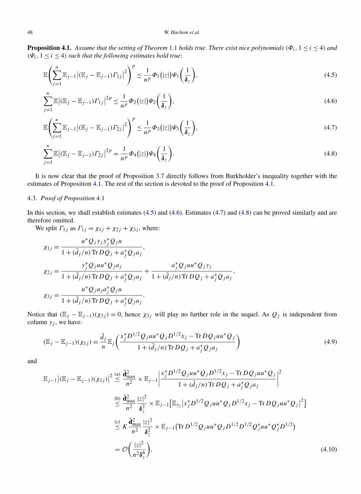
Proposition 4.1. Assume that the setting of Theorem 1.1 holds true. There exist nice polynomials (Φi,1 ≤ i ≤ 4) and(Ψi,1 ≤ i ≤ 4) such that the following estimates hold true:
E
(n∑
j=1
Ej−1∣∣(Ej − Ej−1)Γ1j
∣∣2)p
≤ 1
npΦ1(|z|)Ψ1
(1
δz
), (4.5)
n∑j=1
E∣∣(Ej − Ej−1)Γ1j
∣∣2p ≤ 1
npΦ2(|z|)Ψ2
(1
δz
), (4.6)
E
(n∑
j=1
Ej−1∣∣(Ej − Ej−1)Γ2j
∣∣2)p
≤ 1
npΦ3(|z|)Ψ3
(1
δz
), (4.7)
n∑j=1
E∣∣(Ej − Ej−1)Γ2j
∣∣2p = 1
npΦ4(|z|)Ψ4
(1
δz
). (4.8)
It is now clear that the proof of Proposition 3.7 directly follows from Burkholder’s inequality together with theestimates of Proposition 4.1. The rest of the section is devoted to the proof of Proposition 4.1.
4.3. Proof of Proposition 4.1
In this section, we shall establish estimates (4.5) and (4.6). Estimates (4.7) and (4.8) can be proved similarly and aretherefore omitted.
We split Γ1j as Γ1j = χ1j + χ2j + χ3j , where:
χ1j = u∗Qjyjy∗j Qju
1 + (dj /n)TrDQj + a∗j Qjaj
,
χ2j = y∗j Qjuu∗Qjaj
1 + (dj /n)TrDQj + a∗j Qjaj
+ a∗j Qjuu∗Qjyj
1 + (dj /n)TrDQj + a∗j Qjaj
,
χ3j = u∗Qjaja∗j Qju
1 + (dj /n)TrDQj + a∗j Qjaj
.
Notice that (Ej − Ej−1)(χ3j ) = 0, hence χ3j will play no further role in the sequel. As Qj is independent fromcolumn yj , we have:
(Ej − Ej−1)(χ1j ) = dj
nEj
(x∗j D1/2Qjuu∗QjD
1/2xj − TrDQjuu∗Qj
1 + (dj /n)TrDQj + a∗j Qjaj
)(4.9)
and
Ej−1∣∣(Ej − Ej−1)(χ1j )
∣∣2 (a)≤ d2max
n2× Ej−1
∣∣∣∣x∗j D1/2Qjuu∗QjD
1/2xj − TrDQjuu∗Qj
1 + (dj /n)TrDQj + a∗j Qjaj
∣∣∣∣2(b)≤ d2
max
n2
|z|2δ2z
× Ej−1[Eyj
∣∣x∗j D1/2Qjuu∗QjD
1/2xj − TrDQjuu∗Qj
∣∣2](c)≤ K
d2max
n2
|z|2δ2z
× Ej−1(TrD1/2Qjuu∗QjD
1/2D1/2Q∗j uu∗Q∗
jD1/2)
= O( |z|2
n2δ6z
), (4.10)
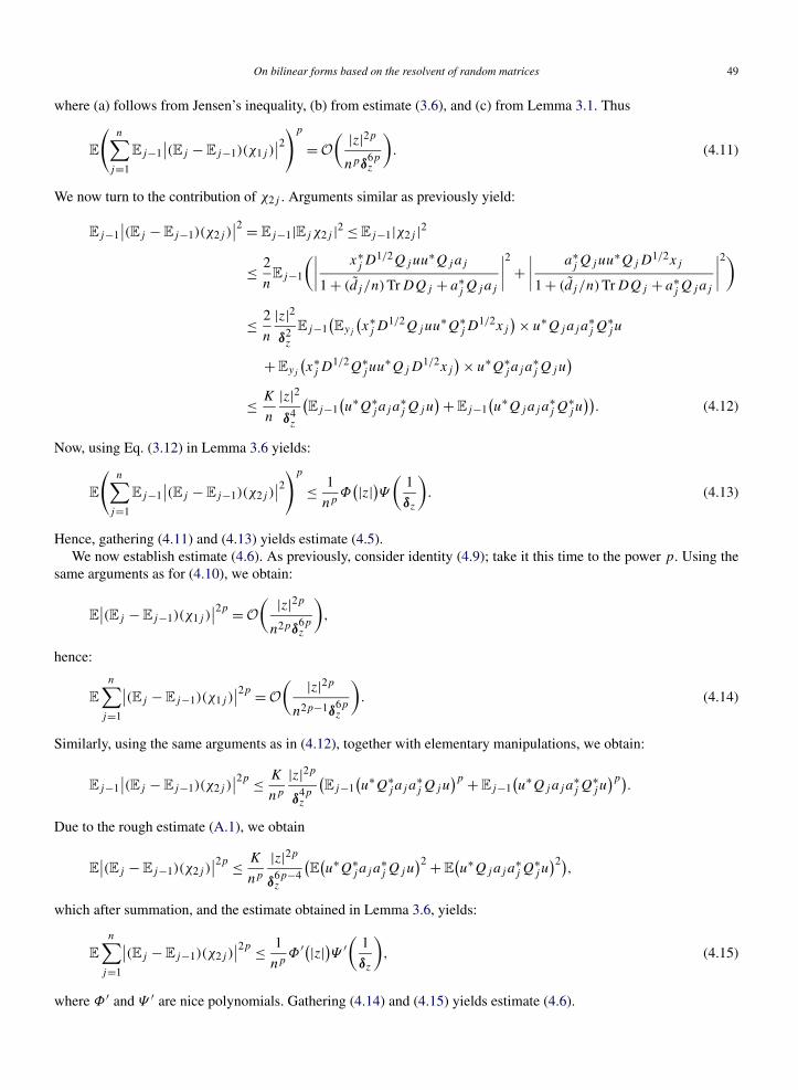
On bilinear forms based on the resolvent of random matrices 49
where (a) follows from Jensen’s inequality, (b) from estimate (3.6), and (c) from Lemma 3.1. Thus
E
(n∑
j=1
Ej−1∣∣(Ej − Ej−1)(χ1j )
∣∣2)p
= O( |z|2p
npδ6pz
). (4.11)
We now turn to the contribution of χ2j . Arguments similar as previously yield:
Ej−1∣∣(Ej − Ej−1)(χ2j )
∣∣2 = Ej−1|Ejχ2j |2 ≤ Ej−1|χ2j |2
≤ 2
nEj−1
(∣∣∣∣ x∗j D1/2Qjuu∗Qjaj
1 + (dj /n)TrDQj + a∗j Qjaj
∣∣∣∣2 +∣∣∣∣ a∗
j Qjuu∗QjD1/2xj
1 + (dj /n)TrDQj + a∗j Qjaj
∣∣∣∣2)
≤ 2
n
|z|2δ2z
Ej−1(Eyj
(x∗j D1/2Qjuu∗Q∗
jD1/2xj
)× u∗Qjaja∗j Q∗
j u
+ Eyj
(x∗j D1/2Q∗
j uu∗QjD1/2xj
)× u∗Q∗j aj a
∗j Qju
)≤ K
n
|z|2δ4z
(Ej−1
(u∗Q∗
j aj a∗j Qju
)+ Ej−1(u∗Qjaja
∗j Q∗
j u))
. (4.12)
Now, using Eq. (3.12) in Lemma 3.6 yields:
E
(n∑
j=1
Ej−1∣∣(Ej − Ej−1)(χ2j )
∣∣2)p
≤ 1
npΦ(|z|)Ψ( 1
δz
). (4.13)
Hence, gathering (4.11) and (4.13) yields estimate (4.5).We now establish estimate (4.6). As previously, consider identity (4.9); take it this time to the power p. Using the
same arguments as for (4.10), we obtain:
E∣∣(Ej − Ej−1)(χ1j )
∣∣2p = O( |z|2p
n2pδ6pz
),
hence:
E
n∑j=1
∣∣(Ej − Ej−1)(χ1j )∣∣2p = O
( |z|2p
n2p−1δ6pz
). (4.14)
Similarly, using the same arguments as in (4.12), together with elementary manipulations, we obtain:
Ej−1∣∣(Ej − Ej−1)(χ2j )
∣∣2p ≤ K
np
|z|2p
δ4pz
(Ej−1
(u∗Q∗
j aj a∗j Qju
)p + Ej−1(u∗Qjaja
∗j Q∗
j u)p)
.
Due to the rough estimate (A.1), we obtain
E∣∣(Ej − Ej−1)(χ2j )
∣∣2p ≤ K
np
|z|2p
δ6p−4z
(E(u∗Q∗
j aj a∗j Qju
)2 + E(u∗Qjaja
∗j Q∗
j u)2)
,
which after summation, and the estimate obtained in Lemma 3.6, yields:
E
n∑j=1
∣∣(Ej − Ej−1)(χ2j )∣∣2p ≤ 1
npΦ ′(|z|)Ψ ′
(1
δz
), (4.15)
where Φ ′ and Ψ ′ are nice polynomials. Gathering (4.14) and (4.15) yields estimate (4.6).

50 W. Hachem et al.
5. Proof of Proposition 3.8
The argument referred to in Section 4.1 still holds true here; therefore it is sufficient to establish, for z ∈ C − R+ and
for a unit vector u:
∣∣u∗(EQ(z) − R(z)
)u∣∣≤ 1√
nΦ(|z|)Ψ( 1
δz
). (5.1)
Recalling that R = [−z(I + αD) + A(I + αD)−1A∗]−1, the resolvent identity yields:
u∗(R − Q)u = u∗R(Q−1 − R−1)Qu
= u∗R(ΣΣ∗ − A(I + αD)−1A∗)Qu + zαu∗RDQu
= u∗R(
n∑j=1
ηjη∗j −
n∑j=1
aja∗j
1 + αdj
)Qu + zαu∗RDQu
(a)=n∑
j=1
u∗Rηjη∗jQju
1 + η∗jQjηj
−n∑
j=1
u∗Raja∗j Qju
1 + αdj
+n∑
j=1
u∗Raja∗j Qjηjη
∗jQju
(1 + η∗jQjηj )(1 + αdj )
−n∑
j=1
dj
nE
(1
1 + η∗jQjηj
)u∗RDQu
�=n∑
j=1
Zj ,
where (a) follows from (3.2) and (3.5), together with the mere definition of α.As usual, we now write ηj = yj + aj , group the terms that compensate one another and split Zj accordingly:
Zj = Z1j + Z2j + Z3j + Z4j ,
where
Z1j = y∗j Qjuu∗Ryj
1 + η∗jQjηj
− dj
nE
(1
1 + η∗jQjηj
)u∗RDQu,
Z2j = (αdj − y∗j Qjyj )u
∗Raja∗j Qju
(1 + η∗jQjηj )(1 + αdj )
,
Z3j = y∗j Qjua∗
j Qjyj × u∗Raj
(1 + η∗jQjηj )(1 + αdj )
,
Z4j = u∗Ryja∗j Qju + u∗Rajy
∗j Qju
1 + η∗jQjηj
− y∗j Qjaju
∗Raja∗j Qju + a∗
j Qjyju∗Raja
∗j Qju
(1 + η∗jQjηj )(1 + αdj )
+ u∗Raja∗j Qjajy
∗j Qju + u∗Raja
∗j Qjyja
∗j Qju
(1 + η∗jQjηj )(1 + αdj )
.
Now, the estimate (5.1) immediately follows from similar estimates for the terms E∑n
j=1 Z j , 1 ≤ ≤ 4.
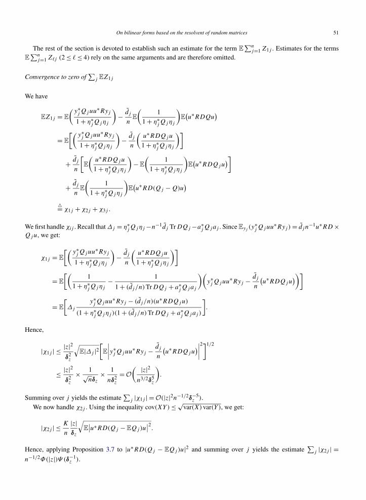
On bilinear forms based on the resolvent of random matrices 51
The rest of the section is devoted to establish such an estimate for the term E∑n
j=1 Z1j . Estimates for the termsE∑n
j=1 Z j (2 ≤ ≤ 4) rely on the same arguments and are therefore omitted.
Convergence to zero of∑
j EZ1j
We have
EZ1j = E
(y∗j Qjuu∗Ryj
1 + η∗jQjηj
)− dj
nE
(1
1 + η∗jQjηj
)E(u∗RDQu
)
= E
[(y∗j Qjuu∗Ryj
1 + η∗jQjηj
)− dj
n
(u∗RDQju
1 + η∗jQjηj
)]
+ dj
n
[E
(u∗RDQju
1 + η∗jQjηj
)− E
(1
1 + η∗jQjηj
)E(u∗RDQju
)]
+ dj
nE
(1
1 + η∗jQjηj
)E(u∗RD(Qj − Q)u
)�= χ1j + χ2j + χ3j .
We first handle χij . Recall that Δj = η∗jQjηj −n−1dj TrDQj −a∗
j Qjaj . Since Eyj(y∗
j Qjuu∗Ryj ) = dj n−1u∗RD ×
Qju, we get:
χ1j = E
[(y∗j Qjuu∗Ryj
1 + η∗jQjηj
)− dj
n
(u∗RDQju
1 + η∗jQjηj
)]
= E
[(1
1 + η∗jQjηj
− 1
1 + (dj /n)TrDQj + a∗j Qjaj
)(y∗j Qjuu∗Ryj − dj
n
(u∗RDQju
))]
= E
[Δj
y∗j Qjuu∗Ryj − (dj /n)(u∗RDQju)
(1 + η∗jQjηj )(1 + (dj /n)TrDQj + a∗
j Qjaj )
].
Hence,
|χ1j | ≤ |z|2δ2z
√E|Δj |2
[E
∣∣∣∣y∗j Qjuu∗Ryj − dj
n
(u∗RDQju
)∣∣∣∣2]1/2
≤ |z|2δ2z
× 1√nδz
× 1
nδ2z
= O( |z|2
n3/2δ5z
).
Summing over j yields the estimate∑
j |χ1j | = O(|z|2n−1/2δ−5z ).
We now handle χ2j . Using the inequality cov(XY) ≤ √var(X)var(Y ), we get:
|χ2j | ≤ K
n
|z|δz
√E∣∣u∗RD(Qj − EQj)u
∣∣2.Hence, applying Proposition 3.7 to |u∗RD(Qj − EQj)u|2 and summing over j yields the estimate
∑j |χ2j | =
n−1/2Φ(|z|)Ψ (δ−1z ).

52 W. Hachem et al.
Let us now handle the term χ3j . Using the decomposition of Qj − Q, Schwarz inequality and the fact that√
ab ≤2−1(a + b) yields
|χ3j | =∣∣∣∣ dj
nE
(1
1 + η∗jQjηj
)E(u∗RD(Qj − Q)u
)∣∣∣∣≤ K
n
|z|2δ2z
(E∣∣u∗RDQjηj
∣∣2 + E∣∣η∗
jQju∣∣2). (5.2)
Now, as:
E∣∣u∗RDQjηj
∣∣2 = Eu∗RDQjyjy∗j Q∗
jDR∗u + Eu∗RDQjaja∗j Q∗
jDR∗u,
E∣∣η∗
jQju∣∣2 = Eu∗Q∗
j yj y∗j Qju + Eu∗Q∗
j aj a∗j Qju,
it remains to sum over j and to apply Lemma 3.6 to get the estimate∑
j |χ3j | = n−1Φ(|z|)Ψ (δ−1z ). Gathering the
partial estimates yields:∣∣∣∣E∑j
Z1j
∣∣∣∣≤ Φ(|z|)Ψ (δ−1z )√
n. (5.3)
6. Proof of Proposition 3.9
As mentioned in Section 4.1, it is sufficient to establish the estimate:
∣∣u∗(R(z) − T (z))u∣∣≤ 1
nΦ(|z|)Ψ( 1
δz
)(6.1)
for z ∈ C − R+ in the case where u has norm one.
6.1. The estimate for u∗(R − T )u
Recall the definitions of δ, δ (1.3), α, α (3.13) and R, R (3.14)–(3.15). Using twice the resolvent identity yields:
u∗(R − T )u = (α − δ)κ1 + (α − δ)κ2, (6.2)
where{κ1 = zu∗RDT u,
κ2 = u∗RA(I + αD)−1D(I + δD)−1A∗T u.
The following bounds are straightforward:
|κ1| ≤ |z|dmax
δ2z
and |κ2| ≤ ‖A‖2dmax
δ2z
× ∥∥(I + αD)−1∥∥× ∥∥(I + δD)−1
∥∥.It remains to control the spectral norms of (I + αD)−1 and (I + δD)−1. Recall that α is the Stieltjes transform of apositive measure with support included in R
+. This in particular implies that Im(zα) > 0 for z ∈ C+. One can check
that
Υj (z) = 1
−z(1 + αdj )
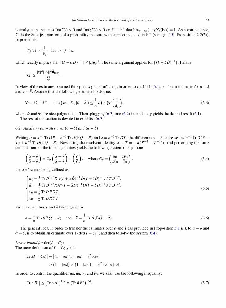
On bilinear forms based on the resolvent of random matrices 53
is analytic and satisfies Im(Υj ) > 0 and Im(zΥj ) > 0 on C+ and that limy→∞(−iyΥj (iy)) = 1. As a consequence,Υj is the Stieltjes transform of a probability measure with support included in R
+ (see e.g. [15], Proposition 2.2(2)).In particular,
∣∣Υj (z)∣∣≤ 1
δz
for 1 ≤ j ≤ n,
which readily implies that ‖(I + αD)−1‖ ≤ |z|δ−1z . The same argument applies for ‖(I + δD)−1‖. Finally,
|κ2| ≤ |z|2‖A‖2dmax
δ4z
.
In view of the estimates obtained for κ1 and κ2, it is sufficient, in order to establish (6.1), to obtain estimates for α − δ
and α − δ. Assume that the following estimate holds true:
∀z ∈ C − R+, max
(|α − δ|, |α − δ|)≤ 1
nΦ(|z|)Ψ( 1
δz
), (6.3)
where Φ and Ψ are nice polynomials. Then, plugging (6.3) into (6.2) immediately yields the desired result (6.1).The rest of the section is devoted to establish (6.3).
6.2. Auxiliary estimates over (α − δ) and (α − δ)
Writing α = n−1 TrDR + n−1 TrD(EQ − R) and δ = n−1 TrDT , the difference α − δ expresses as n−1 TrD(R −T ) + n−1 TrD(EQ − R). Now using the resolvent identity R − T = −R(R−1 − T −1)T and performing the samecomputation for the tilded quantities yields the following system of equations:(
α − δ
α − δ
)= C0
(α − δ
α − δ
)+(
ε
ε
), where C0 =
(u0 zv0zv0 u0
), (6.4)
the coefficients being defined as:⎧⎪⎪⎪⎪⎨⎪⎪⎪⎪⎩
u0 = 1n
TrD1/2RA(I + αD)−1D(I + δD)−1A∗T D1/2,
u0 = 1n
Tr D1/2RA∗(I + αD)−1D(I + δD)−1AT D1/2,
v0 = 1n
TrDRDT,
v0 = 1n
Tr DRDT
(6.5)
and the quantities ε and ε being given by:
ε = 1
nTrD(EQ − R) and ε = 1
nTr D(EQ − R). (6.6)
The general idea, in order to transfer the estimates over ε and ε (as provided in Proposition 3.8(ii)), to α − δ andα − δ, is to obtain an estimate over 1/det(I − C0), and then to solve the system (6.4).
Lower bound for det(I − C0)
The mere definition of I − C0 yields∣∣det(I − C0)∣∣ = ∣∣(1 − u0)(1 − u0) − z2v0v0
∣∣≥ (
1 − |u0|)× (
1 − |u0|)− |z|2|v0| × |v0|.
In order to control the quantities u0, u0, v0 and v0, we shall use the following inequality:∣∣TrAB∗∣∣≤ (TrAA∗)1/2 × (
TrBB∗)1/2, (6.7)
54 W. Hachem et al.
together with the following quantities:⎧⎪⎪⎪⎪⎨⎪⎪⎪⎪⎩
u1 = 1n
TrDT A(I + δ∗D
)−1D(I + δD)−1A∗T ∗,
u1 = 1n
Tr DT A∗(I + δD)−1D(I + δ∗D
)−1AT ∗,
v1 = 1n
TrDT DT ∗,v1 = 1
nTr DT DT ∗
and ⎧⎪⎪⎪⎪⎨⎪⎪⎪⎪⎩
u2 = 1n
TrDRA(I + α∗D
)−1D(I + αD)−1A∗R∗,
u2 = 1n
Tr DRA∗(I + αD)−1D(I + α∗D
)−1AR∗,
v2 = 1n
TrDRDR∗,v2 = 1
nTr DRDR∗.
(6.8)
Using (6.7) together with identity (I + δD)−1A∗T = T A∗(I + δD)−1 (and similar ones for related quantities), weobtain:
|u0| ≤ (u1u2)1/2, |u0| ≤ (u1u2)
1/2, |v0| ≤ (v1v2)1/2, |v0| ≤ (v1v2)
1/2,
hence the lower bound:∣∣det(I − C0)∣∣≥ (
1 − (u1u2)1/2)(1 − (u1u2)
1/2)− |z|2(v1v2v1v2)1/2. (6.9)
Notice that it is not proved yet that the right-hand side of the previous inequality is non-negative.In order to handle estimate (6.9), we shall rely on the following proposition.
Proposition 6.1. Consider the nonnegative real numbers xi, yi, si , ti (i = 1,2). Assume that:
xi ≤ 1, yi ≤ 1 and (1 − xi)(1 − yi) − si ti ≥ 0 for i = 1,2.
Then:(1 − √
x1x2)(
1 − √y1y2
)− √s1s2t1t2
≥√(1 − x1)(1 − y1) − s1t1
√(1 − x2)(1 − y2) − s2t2.
Proof. If a ≥ c (≥ 0) and b ≥ d (≥ 0), then:√
ab − √cd ≥ √
a − c√
b − d.
To prove this, simply take the difference of the squares. Applying once this inequality yields 1 − √x1x2 ≥√
(1 − x1)(1 − x2), hence:(1 − √
x1x2)(
1 − √y1y2
)− √s1s2t1t2 ≥√
(1 − x1)(1 − x2)(1 − y1)(1 − y2) − √s1s2t1t2.
Applying again the first inequality yields then the desired result. �
Our goal is to apply Proposition 6.1 to (6.9). The main idea, in order to fulfill assumptions of Proposition 6.1 (atleast on some portions of C − R
+), is to consider the quantities of interest, i.e. ui, ui , vi, vi (i = 1,2) as coefficientsof linear systems whose determinants are the desired quantities (1 − ui)(1 − ui ) − |z|2vi vi .
Consider the following matrices:
Ci(z) =(
ui vi
|z|2vi ui
), i = 1,2.
The following proposition holds true:
On bilinear forms based on the resolvent of random matrices 55
Proposition 6.2. Assume that z ∈ C − R+. Then:
(i) The following holds true: 1 − u1(z) ≥ 0 and 1 − u1(z) ≥ 0. Moreover, there exists positive constants K,η suchthat:
det(I − C1(z)
)≥ Kδ8z
(η2 + |z|2)4.
(ii) There exist nice polynomials Φ and Ψ and a set
En ={z ∈ C
+,1
nΦ(|z|)Ψ( 1
δz
)≤ 1/2
},
such that for every z ∈ En, 1 − u2(z) ≥ 0, 1 − u2(z) ≥ 0, and
det(I − C2) ≥ Kδ8z
(η2 + |z|2)4,
where K,η are positive constants.
Proof of Proposition 6.2 is postponed to Appendix B.We are now in position to establish the following estimate:
∀z ∈ En, max(|α − δ|, |α − δ|)≤ 1
nΦ(|z|)Ψ( 1
δz
). (6.10)
Assume z ∈ En. Thanks to Proposition 6.2, assumptions of Proposition 6.1 are fulfilled by ui, ui , vi and vi , and (6.9)yields:
det(I − C0) ≥√det(I − C1)
√det(I − C2) ≥ K
δ8z
(η2 + |z|2)4, (6.11)
where K,η are nice constants.Solving now the system (6.4), we obtain:{
α − δ = (det(I − C0)
)−1((1 − u0)ε + zv0ε
),
α − δ = (det(I − C0)
)−1((1 − u0)ε + zv0ε
).
It remains to use (6.11), Proposition 3.8(ii), and obvious bounds over u0, u0, v0 and v0 to conclude and obtain (6.10).We turn out to the case where z ∈ C − R
+ − En, and rely on the same argument as in Haagerup and Thorbjornsen[12] (see also [8]). In this case,
1
nΦ(|z|)Ψ (δ−1
z
)≥ 1
2.
As |α − δ| = |n−1 TrD(EQ − T )| ≤ 2�+dmaxδ−1z , we obtain:
∀z ∈ C − R+ − En, |α − δ| ≤ 2�+dmax
δz
× 2Φ(|z|)Ψ (1/δz)
n;
a similar estimate holds for α − δ for z /∈ En. Gathering the cases where z ∈ En and z /∈ En yields (6.3).
56 W. Hachem et al.
Appendix A: Remaining proofs for Section 3
Proof of Lemma 3.5. Note that it is sufficient to establish the result for a vector u with norm one (which is assumedin the sequel). The general result follows by considering u/‖u‖.
We proceed by induction over p. Let p = 1 and consider:
0 ≤ E
n∑j=1
Ej−1u∗Qaja
∗j Q∗u = Eu∗QAA∗Q∗u ≤ a2
maxE‖Q‖2.
As ‖Q‖ ≤ δ−1z , we obtain the desired bound.
Now, write
E
∣∣∣∣∣n∑
j=1
Ej−1(u∗Qaja
∗j Q∗u
)∣∣∣∣∣p
=∑
j1,...,jp
E[Ej1−1
(u∗Qaj1a
∗j1
Q∗u) · · ·Ejp−1
(u∗Qajpa∗
jpQ∗u
)]
≤ p!∑
j1≤···≤jp
E[Ej1−1
(u∗Qaj1a
∗j1
Q∗u) · · ·Ejp−1
(u∗Qajpa∗
jpQ∗u
)]
= p!∑
j1≤···≤jp
E
[Ejp−1
(u∗Qajpa∗
jpQ∗u
)p−1∏k=1
Ejk−1(u∗Qajk
a∗jk
Q∗u)
︸ ︷︷ ︸Fjp−1 measurable
]
= p!∑
j1≤···≤jp−1
E
[n∑
jp=jp−1
(u∗Qajpa∗
jpQ∗u
)p−1∏k=1
Ejk−1(u∗Qajk
a∗jk
Q∗u)]
(a)≤ p!a2max
δ2z
E
∣∣∣∣∣n∑
j=1
Ej−1(u∗Qaja
∗j Q∗u
)∣∣∣∣∣p−1
,
where (a) follows from the fact that
n∑jp=jp−1
(u∗Qajpa∗
jpQ∗u
)≤n∑
jp=1
(u∗Qajpa∗
jpQ∗u
)≤ a2max
δ2z
.
It remains to plug the induction assumption to conclude. Hence (3.9) is established.In order to establish (3.10), one may use the same arguments as previously together with the identity QΣΣ∗ =
I + zQ, which yields the factor |z|p in estimate (3.10). �
Proof of Lemma 3.6. We prove the lemma in the case where ‖u‖ = 1, the general result readily follows by consider-ing u/‖u‖.
Write u∗Qjaja∗j Q∗
j u = χ1j + χ2j + χ3j + χ4j with:
χ1j = u∗(Qj − Q)aja∗j (Qj − Q)∗u,
χ2j = u∗Qaja∗j Q∗u,
χ3j = u∗(Qj − Q)aja∗j Q∗u,
χ4j = u∗Qaja∗j (Qj − Q)∗u.
On bilinear forms based on the resolvent of random matrices 57
Hence,
n∑j=1
E(u∗Qjaja
∗j Q∗
j u)2 ≤
n∑j=1
Eχ21j +
n∑j=1
Eχ22j +
n∑j=1
E|χ3j |2 +n∑
j=1
E|χ4j |2.
Notice that:
E|χ3j |2 ≤ 1
2
(Eχ2
1j + Eχ22j
)and E|χ4j |2 ≤ 1
2
(Eχ2
1j + Eχ22j
).
Note that using the facts that aja∗j ≤ AA∗ and ηjη
∗j ≤ ΣΣ∗ together with the identity QΣΣ∗ = I + zQ yield the
rough but useful estimates:
u∗Qaja∗j Q∗u = O
(δ−2z
)and u∗Qηjη
∗jQ
∗u = O( |z|
δ2z
). (A.1)
We first begin by the contribution of∑
j Eχ22j :
n∑j=1
χ22j =
n∑j=1
u∗Qaja∗j Q∗u × u∗Qaja
∗j Q∗u
≤n∑
j=1
u∗Qaja∗j Q∗u × u∗QAA∗Q∗u
≤ (u∗QAA∗Q∗u
)2 = O(δ−4z
)≤ Φ2(|z|)Ψ2
(1
δz
). (A.2)
Similarly,
n∑j=1
(u∗Qηjη
∗jQ
∗u)2 = O
( |z|2δ4z
). (A.3)
We now turn to the contribution of∑
j Eχ21j . Using the decompositions (3.2), (3.3) and (3.4), χ1j writes:
χ1j =∣∣∣∣1 + η∗
jQjηj
1 − η∗jQηj
∣∣∣∣× ∣∣u∗Qηjη∗jQaja
∗j Q∗ηjη
∗jQ
∗u∣∣
= ∣∣1 + η∗jQjηj
∣∣× ∣∣u∗Qηjη∗jQ
∗u∣∣× ∣∣∣∣a∗
j Q∗ηjη∗jQaj
1 − η∗jQηj
∣∣∣∣. (A.4)
We first prove that
a∗j Q∗ηjη
∗jQaj
1 − η∗jQηj
= O( |z|
δ2z
). (A.5)
In fact:∣∣∣∣a∗j Q∗ηjη
∗jQaj
1 − η∗jQηj
∣∣∣∣ ≤∣∣∣∣a∗
j Q∗ηjη∗jQ
∗aj
1 − η∗jQηj
∣∣∣∣+∣∣∣∣a∗
j Q∗ηjη∗j (Q − Q∗)aj
1 − η∗jQηj
∣∣∣∣(a)≤ ∣∣a∗
j (Qj − Q)∗aj
∣∣+ 2∣∣Im(z)
∣∣∣∣a∗j (Qj − Q)Qaj
∣∣= O
(1
δz
)+ O
( |z|δ2z
)= O
( |z|δ2z
),
58 W. Hachem et al.
where we use the fact that Q − Q∗ = 2i Im(z)Q∗Q to obtain (a). Now,
∣∣1 + η∗jQjηj
∣∣≤ 1 + |Δj | +∣∣∣∣ dj
nTrDQj + a∗
j Qjaj
∣∣∣∣. (A.6)
Since |n−1dj TrDQj + a∗j Qjaj | = O(δ−1
z ), we obtain:
n∑j=1
Eχ21j =
(O( |z|2
δ4z
)+ O
( |z|2δ6z
))×
n∑j=1
E(u∗Qηjη
∗jQ
∗u)2
+ O( |z|2
δ4z
)×
n∑j=1
E(u∗Qηjη
∗jQ
∗u)2 × |Δj |2
(a)= O( |z|4
δ8z
)+ O
( |z|4δ10z
)+ O
( |z|4δ8z
)×
n∑j=1
E|Δj |2
(b)= O( |z|4
δ8z
)+ O
( |z|4δ10z
)
≤ Φ1(|z|)Ψ1
(1
δz
),
where (a) follows from (A.3) and (A.1) and (b), from Corollary 3.2.It remains to gather the contributions of χ1j , χ2j , χ3j and χ4j to get:
n∑j=1
E(u∗Qjaja
∗j Q∗
j u)2 ≤ 2Φ1
(|z|)Ψ1
(1
δz
)+ 2Φ2
(|z|)Ψ2
(1
δz
)(a)≤ Φ
(|z|)Ψ( 1
δz
),
where (a) follows from (3.7). Equation (3.11) is proved.In order to prove (3.12), first note that:
E
(n∑
j=1
Ej−1(u∗Qjaja
∗j Q∗
j u))p
≤ K
(E
∣∣∣∣∣n∑
j=1
Ej−1χ1j
∣∣∣∣∣p
+ E
∣∣∣∣∣n∑
j=1
Ej−1χ2j
∣∣∣∣∣p
+ E
∣∣∣∣∣n∑
j=1
Ej−1χ3j
∣∣∣∣∣p
+ E
∣∣∣∣∣n∑
j=1
Ej−1χ4j
∣∣∣∣∣p)
.
Hence, it remains to evaluate the contributions of each term. Using decomposition (A.4) together with the esti-mate (A.5), we obtain:
E
∣∣∣∣∣n∑
j=1
Ej−1χ1j
∣∣∣∣∣p
= O( |z|p
δ2pz
)× E
(n∑
j=1
Ej−1∣∣1 + η∗
jQjηj
∣∣× u∗Qηjη∗jQ
∗u)p
.
Using (A.6) together with (3.10) yields:
E
∣∣∣∣∣n∑
j=1
Ej−1χ1j
∣∣∣∣∣p
= O( |z|2p
δ4pz
)+ O
( |z|2p
δ5pz
)+ O
( |z|pδ
2pz
)× E
∣∣∣∣∣n∑
j=1
Ej−1(|Δj | × u∗Qηjη
∗jQ
∗u)∣∣∣∣∣
p
.

On bilinear forms based on the resolvent of random matrices 59
Combining standard inequalities (Cauchy–Schwarz, |∑j aj bj | ≤ (∑
j a2j )
1/2(∑
j b2j )
1/2, and Cauchy–Schwarzagain), we obtain:
E
(n∑
j=1
Ej−1(|Δj | × u∗Qηjη
∗jQ
∗u))p
≤[
E
(n∑
j=1
Ej−1(u∗Qηjη
∗jQ
∗u)2
)p
× E
(n∑
j=1
Ej−1|Δj |2)p]1/2
(a)= O( |z|p
δ3pz
),
where (a) follows from (A.1), Corollary 3.2 and (3.10). Finally,
E
∣∣∣∣∣n∑
j=1
Ej−1χ1j
∣∣∣∣∣p
= O( |z|2p
δ4pz
)+ O
( |z|2p
δ5pz
)+ O
( |z|2p
δ5pz
)≤ Φ1
(|z|)Ψ1(δ−1z
). (A.7)
Equation (3.9) directly yields the estimate:
E
∣∣∣∣∣n∑
j=1
Ej−1χ2j
∣∣∣∣∣p
= O(
1
δ2pz
)≤ Φ2
(|z|)Ψ2(δ−1z
). (A.8)
Finally,
E
∣∣∣∣∣n∑
j=1
Ej−1χ3j
∣∣∣∣∣p
≤(
E
∣∣∣∣∣n∑
j=1
Ej−1χ1j
∣∣∣∣∣p
E
∣∣∣∣∣n∑
j=1
Ej−1χ2j
∣∣∣∣∣p)1/2
≤ Φ3(|z|)Ψ3
(1
δz
). (A.9)
A corresponding inequality exists for E|∑Ej−1χ4j |p , obtain:
E
∣∣∣∣∣n∑
j=1
Ej−1χ4j
∣∣∣∣∣p
≤ Φ4(|z|)Ψ4
(1
δz
). (A.10)
Gathering (A.7), (A.8), (A.9) and (A.10), we end up with (3.12), and Lemma 3.6 is proved. �
Appendix B: Remaining proofs for Section 6
Proof of Proposition 6.2(i). Recall that δ = 1n
TrDT and δ = 1n
Tr DT . We consider first the case where z ∈ C+ ∪C−.We have
Im(δ) = 1
2inTrDT
(T −∗ − T −1)T ∗ and Im(zδ) = 1
2inTr D(zT )
[(zT )−∗ − (zT )−1](zT )∗.
Developing the previous identities, we end up with the system:
(I − C1)
(Im(δ)
Im(zδ)
)= Im(z)
(w1(z)
x1(z)
), (B.1)
where{w1(z) = 1
nTrDT T ∗ (> 0),
x1(z) = 1n
Tr DT A∗(I + δD)−1(I + δ∗D
)−1AT ∗ (> 0).

60 W. Hachem et al.
By developing the first equation of this system, and by recalling that δ(z) is the Stieltjes transform of a positivemeasure μn with support included in R
+, we obtain
1 − u1 = w1Im(z)
Im(δ)+ v1
Im(zδ)
Im(δ)≥ w1
Im(z)
Im(δ)≥ 0.
Replacing (Im(δ), Im(zδ)) with (Im(δ), Im(zδ)) and repeating the same argument, we obtain
1 − u1 = w1Im(z)
Im(δ)+ v1
Im(zδ)
Im(δ)≥ w1
Im(z)
Im(δ)≥ 0.
By continuity of u1(z) and u1(z) at any point of the open real negative axis, we have 1 − u1 ≥ 0 and 1 − u1 ≥ 0 forany z ∈ C − R
+. The first two inequalities in the statement of Proposition 6.2(i) are proven.By applying Cramer’s rule ([16], Section 0.8.3) where the first column of I − C1 is replaced with the right-hand
member of (B.1), we obtain
det(I − C1) = (1 − u1)w1Im(z)
Im(δ)+ v1x1
Im(z)
Im(δ)≥ (1 − u1)w1
Im(z)
Im(δ)≥ w1w1
Im(z)
Im(δ)
Im(z)
Im(δ). (B.2)
Using the fact that the positive measure μn is supported by R+ and has a total mass n−1 TrD, we have
0 ≤ Im(δ)
Im(z)=∫
1
|t − z|2 μn(dt) ≤ 1
δ2z
1
nTrD ≤ �+dmax
δ2z
and 0 ≤ Im(δ)
Im(z)≤ dmax
δ2z
. (B.3)
In order to find a lower bound on w1 and w1, we begin by finding a lower bound on |δ|.A computation similar to [15], Lemma C.1, shows that the sequence of measures (μn) is tight. Hence there exists
η > 0 such that:
μn[0, η] ≥ 1
2
1
nTrD ≥ �−dmin
2.
We have
|δ| ≥ ∣∣Im(δ)∣∣= ∣∣Im(z)
∣∣ ∫ μn(dt)
|t − z|2 ≥ ∣∣Im(z)∣∣ ∫ η
0
μn(dt)
2(t2 + |z|2) ≥ ∣∣Im(z)∣∣ �−dmin
4(η2 + |z|2) . (B.4)
Furthermore, when Re(z) < 0, we have
|δ| ≥ Re(δ) =∫
t − Re(z)
|t − z|2 μn(dt) ≥ −Re(z)∫
μn(dt)
|t − z|2 ≥ −Re(z)�−dmin
4(η2 + |z|2) ,
which results in
|δ| ≥ δz
�−dmin
4(η2 + |z|2) .
We can now find a lower bound to w1:
w1 = 1
nTrDT T ∗ = 1
n
N∑i=1
di
N∑j=1
|Tij |2 = 1
nTrD
N∑i=1
κi
N∑j=1
|Tij |2 with κi = di
TrD
(a)≥ 1
nTrD
(N∑
i=1
κi
(N∑
j=1
|Tij |2)1/2)2
≥ 1
nTrD
(N∑
i=1
κi |Tii |)2
≥ 1
nTrD
∣∣∣∣∣N∑
i=1
κiTii
∣∣∣∣∣2
= |δ|2(1/n)TrD
≥ (δz�−dmin)
2
16�+dmax(η2 + |z|2)2,
On bilinear forms based on the resolvent of random matrices 61
where (a) follows by convexity. A similar computation yields w1 ≥ (δzdmin)2/(16dmax(η
2 + |z|2)2) where η is apositive constant. Grouping these estimates with those in (B.3) and plugging them into (B.2), we obtain
det(I − C1) ≥ δ8z(�
−dmindmin)2
256(�+dmaxdmax)2(η2 + |z|2)2(η2 + |z|2)2
≥ Kδ8z
(max(η, η)2 + |z|2)4,
where K is a nice constant. The same bound holds for z ∈ (−∞,0) by continuity of det(I − C1(z)) at any point ofthe open real negative axis. �
Proof of Proposition 6.2(ii). Recall that
εn = 1
nTrD(EQ − R).
We first establish useful estimates.
Lemma B.1. There exists nice polynomials Φ and Ψ such that:∣∣∣∣ Im(εn(z))
Im(z)
∣∣∣∣≤ 1
nΦ(|z|)Ψ( 1
δz
)and
∣∣∣∣ Im(zεn(z))
Im(z)
∣∣∣∣≤ 1
nΦ(|z|)Ψ( 1
δz
)for z ∈ C − R
+.
Proof. We prove the first inequality. By Proposition 3.8(ii), the sequence of functions (εn) satisfies over C − R+∣∣εn(z)
∣∣≤ 1
nΦ(|z|)Ψ( 1
δz
),
where Φ and Ψ are nice polynomials. Let R be the region of the complex plane defined as R = {z: Re(z) <
0, | Im(z)| < −Re(z)/2}. If z ∈ C − R+ − R, then | Im(z)| ≥ δz/
√5, therefore | Imε(z)/ Im z| ≤ n−1
√5δ−1
z Φ(|z|) ×Ψ (δ−1
z ) and the result is proven. Assume now that z ∈ R. In this case, z belongs to the open disc Dz centered at Re(z)
with radius −Re(z)/2. For any u ∈ Dz, we have |ε(u)| ≤ n−1Φ(|u|)Ψ (|u|−1). Moreover,
∀u ∈ Dz,δz√
5≤ −Re(z)
2≤ |u| ≤ −3 Re(z)
2≤ 3|z|
2.
As Φ(x) is increasing and Ψ (1/x) is decreasing in x > 0, we obtain:
∣∣εn(u)∣∣≤ 1
nΦ
(3|z|
2
)Ψ
(√5
δz
)for u ∈ Dz. (B.5)
The function ε is holomorphic on Dz. Consider the function: Applying Lemma 3.4 with
f (ζ ) = ε(|Re(z)/2|ζ + Re(z)) − ε(Re(z))
supu∈Dz|ε(u) − ε(Re(z))| .
Let ζ = i2 Im(z)/Re(z), apply Lemma 3.4, and use (B.5). This yields:
∣∣ε(z) − ε(Re(z)
)∣∣≤ 2| Im(z)||Re(z)| × 1
nΦ(|z|)Ψ( 1
δz
)≤
√5| Im(z)|
δz
× 1
nΦ(|z|)Ψ( 1
δz
),
where Φ and Ψ are nice polynomials. As Im(ε(Re(z))) = 0, we obtain∣∣∣∣ Im(εn(z))
Im(z)
∣∣∣∣≤∣∣∣∣ε(z) − ε(Re(z))
Im(z)
∣∣∣∣≤√
5
δznΦ(|z|)Ψ( 1
δz
).
62 W. Hachem et al.
This proves the first inequality. The second one can be proved similarly. �
We now tackle the proof of Proposition 6.2(ii), following closely the line of the proof of Proposition 6.2(i). Recallthat α = 1
nTrDEQ, α = 1
nTr DEQ, ε = 1
nTrD(EQ − R) and ε = 1
nTr D(EQ − R). We begin by establishing the
lower bound on det(I −C2). Assume that z ∈ C+∪C
−. Writing α = 1n
TrDR+ε and α = 1n
Tr DR+ ε and developingIm(α) and Im(zα) with the help of the resolvent identity, we get the following system:
(I − C2)
(Im(α)
Im(zα)
)= Im(z)
(w2(z)
x2(z)
)+(
Im(ε)
Im(zε)
),
where w2(z) = 1n
TrDRR∗ and x2(z) > 0. Let w2 = n−1 Tr DRR∗. Using the same arguments as in the proof ofProposition 6.2(i), we obtain
1 − u2 = w2Im(z)
Im(α)+ v2
Im(zα)
Im(α)+ Im(ε)
Im(α)≥ w2
Im(z)
Im(α)+ Im(ε)
Im(α), (B.6)
1 − u2 = w2Im(z)
Im(α)+ v2
Im(zα)
Im(α)+ Im(ε)
Im(α)≥ w2
Im(z)
Im(α)+ Im(ε)
Im(α), (B.7)
det(I − C2) ≥ w2w2Im(z)
Im(α)
Im(z)
Im(α)+ w2
Im(z)
Im(α)
Im(ε)
Im(α)+ (1 − u2)
Im(ε)
Im(α)+ v2
Im(zε)
Im(α)
�= w2w2Im(z)
Im(α)
Im(z)
Im(α)+ e(z). (B.8)
We now find an upper bound on the perturbation term e(z). To this end, we have 0 ≤ w2 ≤ �+dmax/δ2z and 0 ≤
v2 ≤ �+d2max/δ
2z . Recalling (6.8), we also have
|1 − u2| ≤ 1 + dmaxdmaxa2max|z|2
δ4z
.
Using the same arguments as in the proof of Proposition 6.2(i) (involving this time the tightness of the measuresassociated with the Stieltjes transforms 1
nTrDR and 1
nTr DR) yields:
Im(z)
Im(α)≤ 4(η2 + |z|2)
�−dmin,
∣∣e(z)∣∣≤ 1
nΦ(|z|)Ψ (δ−1
z
),
Im(z)
Im(α)≤ 4(η2 + |z|2)
�−dmin
for every z ∈ C+ ∪ C
−, where η,K are positive constants, and Φ and Ψ , nice polynomials.Finally, we can state that there exist nice polynomials Φ and Ψ such that:
det(I − C2) ≥ Kδ8z
(η2 + |z|2)4
(1 − 1
nΦ(|z|)Ψ( 1
δz
)).
By continuity of det(I − C2(z)) at any point of the open real negative axis, this inequality is true for any z ∈ C − R+.
Denote by En the set:
En ={z ∈ C − R
+,1
nΦ(|z|)Ψ( 1
δz
)≤ 1/2
}.
If z ∈ En, then det(I − C2) is readily lower-bounded by the quantity stated in Proposition 6.2(ii).By considering inequalities (B.6) and (B.7) and by possibly modifying the polynomials Φ and Ψ , we have 1−u2 ≥
0 and 1 − u2 ≥ 0 for z ∈ En. The proof of Proposition 6.2(ii) is completed. �

On bilinear forms based on the resolvent of random matrices 63
Acknowledgment
This work was partially supported by the Agence Nationale de la Recherche (France), project SESAME n◦ANR-07-MDCO-012-01.
References
[1] C. Artigue and P. Loubaton. On the precoder design of flat fading MIMO systems equipped with MMSE receivers: A large-system approach.IEEE Trans. Inform. Theory 57 (2011) 4138–4155.
[2] Z. D. Bai, B. Q. Miao and G. M. Pan. On asymptotics of eigenvectors of large sample covariance matrix. Ann. Probab. 35 (2007) 1532–1572.MR2330979
[3] Z. D. Bai and J. W. Silverstein. No eigenvalues outside the support of the limiting spectral distribution of large-dimensional sample covariancematrices. Ann. Probab. 26 (1998) 316–345. MR1617051
[4] Z. D. Bai and J. W. Silverstein. Exact separation of eigenvalues of large-dimensional sample covariance matrices. Ann. Probab. 27 (1999)1536–1555. MR1733159
[5] Z. Bai and J. W. Silverstein. No eigenvalues outside the support of the limiting spectral distribution of information-plus-noise type matrices.Random Matrices Theory Appl. 1 (2012) 1150004. MR2930382
[6] F. Benaych-Georges and R. N. Rao. The eigenvalues and eigenvectors of finite, low rank perturbations of large random matrices. Preprint,2009. Available at arXiv:0910.2120.
[7] R. B. Dozier and J. W. Silverstein. On the empirical distribution of eigenvalues of large dimensional information-plus-noise-type matrices.J. Multivariate Anal. 98 (2007) 678–694. MR2322123
[8] M. Capitaine, C. Donati-Martin and D. Féral. The largest eigenvalues of finite rank deformation of large Wigner matrices: Convergence andnonuniversality of the fluctuations. Ann. Probab. 37 (2009) 1–47. MR2489158
[9] J. Dumont, W. Hachem, S. Lasaulce, P. Loubaton and J. Najim. On the capacity achieving covariance matrix for Rician MIMO channels: Anasymptotic approach. IEEE Trans. Inform. Theory 56 (2010) 1048–1069. MR2723661
[10] L. Erdös, H.-T. Yau and J. Yin. Rigidity of eigenvalues of generalized Wigner matrices. Unpublished manuscript, 2010. Available athttp://arxiv.org/pdf/1007.4652.
[11] V. L. Girko. An Introduction to Statistical Analysis of Random Arrays. VSP, Utrecht, 1998. MR1694087[12] U. Haagerup and S. Thorbjørnsen. A new application of random matrices: Ext(C∗
red(F2)) is not a group. Ann. of Math. (2) 162 (2005)711–775. MR2183281
[13] W. Hachem, M. Kharouf, J. Najim and J. Silverstein. A CLT for information-theoretic statistics of non-centered Gram random matrices.Random Matrices Theory Appl. 1 (2012) 1150010. MR2934716
[14] W. Hachem, P. Loubaton and J. Najim. The empirical distribution of the eigenvalues of a Gram matrix with a given variance profile. Ann.Inst. Henri Poincaré Probab. Stat. 42 (2006) 649–670. MR2269232
[15] W. Hachem, P. Loubaton and J. Najim. Deterministic equivalents for certain functionals of large random matrices. Ann. Appl. Probab. 17(2007) 875–930. MR2326235
[16] R. A. Horn and C. R. Johnson. Topics in Matrix Analysis. Cambridge Univ. Press, Cambridge, 1994. MR1288752[17] A. Kammoun, M. Kharouf, W. Hachem, J. Najim and A. El Kharroubi. On the fluctuations of the mutual information for non centered
MIMO channels: The non Gaussian case. In Proc. IEEE International Workshop on Signal Processing Advances in Wireless Communications(SPAWC), 2010.
[18] V. A. Marcenko and L. A. Pastur. Distribution of eigenvalues in certain sets of random matrices. Mat. Sb. (N.S.) 72 (1967) 507–536.MR0208649
[19] X. Mestre. Improved estimation of eigenvalues and eigenvectors of covariance matrices using their sample estimates. IEEE Trans. Inform.Theory 54 (2008) 5113–5129. MR2589886
[20] X. Mestre. On the asymptotic behavior of the sample estimates of eigenvalues and eigenvectors of covariance matrices. IEEE Trans. SignalProcess. 56 (2008) 5353–5368. MR2472837
[21] X. Mestre and M. A. Lagunas. Modified subspace algorithms for DOA estimation with large arrays. IEEE Trans. Signal Process. 56 (2008)598–614. MR2445537
[22] W. Rudin. Real and Complex Analysis, 3rd edition. McGraw-Hill, New York, 1986.[23] J. W. Silverstein. Strong convergence of the empirical distribution of eigenvalues of large-dimensional random matrices. J. Multivariate Anal.
55 (1995) 331–339. MR1370408[24] J. W. Silverstein and Z. D. Bai. On the empirical distribution of eigenvalues of a class of large-dimensional random matrices. J. Multivariate
Anal. 54 (1995) 175–192. MR1345534[25] P. Vallet, P. Loubaton and X. Mestre. Improved subspace estimation for multivariate observations of high dimension: The deterministic signals
case. IEEE Trans. Inform. Theory 58 (2012) 1043–1068.