Czado, Delwarde, Denuit:

Bayesian Poisson Log-Bilinear Mortality Projections

Sonderforschungsbereich 386, Paper 398 (2004)

Online unter: http://epub.ub.uni-muenchen.de/

Projektpartner

BAYESIAN POISSON LOG-BILINEAR MORTALITYPROJECTIONS

CLAUDIA CZADO†, ANTOINE DELWARDE‡ & MICHEL DENUIT∗,‡

†SCA Zentrum Mathematik

Technische Universitat MunchenD-85748 Garching bei Munich, Germany

‡Institut des Sciences Actuarielles

Universite Catholique de LouvainB-1348 Louvain-la-Neuve, Belgium

∗Institut de StatistiqueUniversite Catholique de Louvain

B-1348 Louvain-la-Neuve, Belgium

September 8, 2004

Abstract

Mortality projections are major concerns for public policy, social security and private in-surance. This paper implements a Bayesian log-bilinear Poisson regression model to forecastmortality. Computations are carried out using Markov Chain Monte Carlo methods in whichthe degree of smoothing is learnt from the data. Comparisons are made with the approachproposed by Brouhns, Denuit & Vermunt (2002a,b), as well as with the original modelof Lee & Carter (1992).

Key words and phrases: projected lifetables, expected remaining lifetimes, Poisson regres-sion, MCMC.

1 Introduction

1.1 Lee-Carter model for mortality projections

Mortality forecasts are used in a wide variety of fields: for health policy making, for directingpharmaceutical research, social security, for retirement fund planning and for life insurance,to name just a few. During the 20th century, it is now well documented that the humanmortality globally declined: in most industrialized countries, mortality at adult and old agesreveals decreasing annual death probabilities.

In this paper, we analyze the changes in mortality as a function of both age x and calendartime t. Henceforth, µx(t) will denote the force of mortality at age x and time t. Throughoutthis paper, we assume that given any integer age x and calendar year t,

µx+ξ(t + τ) = µx(t) for 0 ≤ ξ, τ < 1. (1.1)

This is best illustrated with the aid of a coordinate system that has calendar time as abscissaand age as coordinate. Such a representation is called a Lexis diagram after the Germandemographer who introduced it. Both time scales are divided into yearly bands, whichpartition the Lexis plane into square segments. Model (1.1) assumes that the mortality rateis constant within each square, but allows it to vary between squares. We denote as Dxt thenumber of deaths recorded at age x during year t, from an exposure-to-risk Ext (that is, Extis the number of person-years from which Dxt occurred).

A powerful and elegant approach to mortality forecasts has been pioneered by Lee &Carter (1992). Those authors proposed a remarkably simple model for mortality projec-tions, specifying a log-bilinear form for the force of mortality µx(t). The method is in essencea relational model

ln µx(t) = αx + βxκt + εx(t) (1.2)

where µx(t) = Dxt/Ext denotes the observed force of mortality at age x during year t, theεx(t)’s are homoskedastic centered error terms and where the parameters are subject to theconstraints ∑

t

κt = 0 and∑

x

βx = 1 (1.3)

ensuring model identification.An important aspect of Lee-Carter methodology is that the time factor κt is intrinsically

viewed as a stochastic process. Box-Jenkins techniques are then used to estimate and forecastκt within an ARIMA time series model. From this forecast of the general level of mortality,the actual age-specific rates are derived using the estimated age effects. This in turn yieldsprojected life expectancies.

For a review of recent applications of the Lee-Carter methodology, we refer the interestedreaders to Lee (2000). It is worth to mention that the Lee-Carter model is used by theUS Census Bureau as a benchmark for their population forecasts, and its use has beenrecommended by the US Social Security Technical Advisory Panels. It appears to be thedeterminant method in the literature.

1

1.2 Poisson log-bilinear model for mortality projections

According to Brillinger (1986) and Alho (2000), the Poisson approximation for thenumber of deaths occurring in a square of the Lexis diagram is plausible. This lead Sithole,Haberman & Verrall (2000) and Renshaw & Haberman (2003a,b) to implement analternative approach to mortality forecasting: calendar time enters the model as a knowncovariate and a regression model based on heteroskedastic Poisson error structures is used.

A closely related model has been proposed by Brouhns, Denuit & Vermunt (2002a,b),keeping the Lee-Carter log-bilinear form for the forces of mortality. Specifically, Brouhnset al. (2002a,b) considered that

Dxt ∼ Poisson(Extµx(t)

)with µx(t) = exp (αx + βxκt) (1.4)

where the parameters are still subjected to the constraints (1.3).There is thus a key difference between Renshaw & Haberman (2003a) and Brouhns

et al. (2002b) that centres on the intepretation of time: in Brouhns et al. (2002b)time is modeled as a factor and under the approach proposed by Renshaw & Haberman(2003) is modelled as a known covariate. We believe that the former approach is preferablesince we do not constrain ex ante the effect of calendar time to some known functional form.

Instead of resorting to SVD for estimating αx, βx and κt, Brouhns et al. (2002a,b)estimated the parameters by maximizing the log-likelihood based on model (1.4). As in theLee-Carter approach, ARIMA models are then used to forecast the κt’s.

1.3 Scope of the paper

In all the papers mentioned above, the modelling still proceeds in two steps: first the mortal-ity index κt is estimated and then it is extrapolated using Box-Jenkins methodology. Possibleincoherence may arise from this two-step procedure. In order to avoid this flaw, we purposeto integrate both steps into a Bayesian model. Bayesian formulations assume some sort ofsmoothness of age and period effects in order to improve estimation and facilitate prediction.Intuitively, we expect smooth variations of the mortality rates over the Lexis plane. In orderto implement this idea, we resort to a Bayesian model in which the prior portion imposessmoothness by relating the underlying mortality rates to each other over the Lexis plane. Asa consequence, the rate estimate in each age-year square “borrows strength” from informa-tion in adjacent squares. An important advantage of incorporating the idea of smoothnessis that it is possible to use the model for purposes of forecasting future mortality rates.

The Bayesian modelling treats all unknown parameters αx, βx and κt as random variablesand derives their distribution conditional upon the known information (Ext, Dxt). Until re-cently, fully Bayesian analyses had been computationally infeasible and approximation meth-ods were often utilized instead. This changed in the early 1990’s with computer-intensiveMarkov Chain Monte Carlo (MCMC) simulation methods (see Chib (2001) for a summaryand Gilks et al. (1996) for applications). The Monte Carlo approach allows for inferencebased on sampling the posterior distribution of the parameters. A particularly attractivefeature of this approach is the ease with which we can then explore the uncertainty associatedwith the estimates and the forecasts.

2

A Bayesian treatment of mortality projections has been proposed by Girosi & King(2003). The approach followed by these authors is nevertheless entirely different from theone adopted in this paper. We refer the reader to the interesting monograph written bythese authors for more details.

1.4 Agenda

Section 2 describes the model and details the prior assumption on each set of parameters.Section 3 derives the MCMC algorithm yielding the a posteriori distribution of the parame-ters. A numerical illustration is discussed in Section 4, where the results obtained with themethodology developed in this paper are compared with former ones.

By convention, vectors and matrices are denoted by bold lower and upper cases, re-spectively. Parameters and hyper-parameters are denoted by Greek letters. All the vectorsare assumed to be column vectors and the superscript ′ indicates transposition. We de-note as xmin, xmin + 1, . . . , xmax the observed age range and as tmin, tmin + 1, . . . , tmax theobserved calendar time range. Moreover, M = xmax − xmin + 1 is the number of differentages considered in the model, and T = tmax − tmin + 1 is the number of calendar years. Wedenote as IM (resp. IT ) the M -dimensional (resp. T -dimensional) identity matrix. Further,X ∼ N ormal(m, σ2) indicates that the random variable X is normally distributed withmean m and variance σ2, while X ∼ N ormald(m,Σ) indicates that the random vector Xis normally distributed with mean vector m and variance-covariance matrix Σ.

2 Model and prior distributions

2.1 Likelihood function

Let us consider the Poisson log-bilinear model (1.4) supplemented with the constraints (1.3)in order to ensure the identifiability of the model. This model comprises three sets ofparameters: α = (αxmin

, ..., αxmax)′, β = (βxmin, ..., βxmax)′ and κ = (κtmin

, ..., κtmax)′. Thelikelihood function associated with the data points (Ext, Dxt), x = xmin, xmin + 1, . . . , xmax

and t = tmin, tmin + 1, . . . , tmax, writes

L(α,β,κ) =∏

x

∏

t

exp(−Ext exp(αx + βxκt)

)(Ext exp(αx + βxκt)

)Dxt

Dxt!

∝∏

x

∏

t

exp(−Ext exp(αx + βxκt) +Dxt(αx + βxκt)

). (2.1)

As usual, the first stage of a Bayesian analysis is to specify a prior probability densityfor the parameters α, β and κ involved in the Poisson log-bilinear model. This prior shouldsupport the local regularities that are believed to exist.

2.2 Prior distribution for the time index κ

The time index κt represents the time trend. The actual forces of mortality change accord-ing to an overall mortality index κt modulated by an age response βx. In the Lee-Carter

3

approach, as well as in its Poisson counterpart, the κt’s are projected using an ARIMAmodel. In that respect, a random walk with drift was found the most appropriate for thedata analyzed by Lee & Carter (1992). In practice, that simple model for κt is usedalmost exclusively and accounts for nearly all real applications.

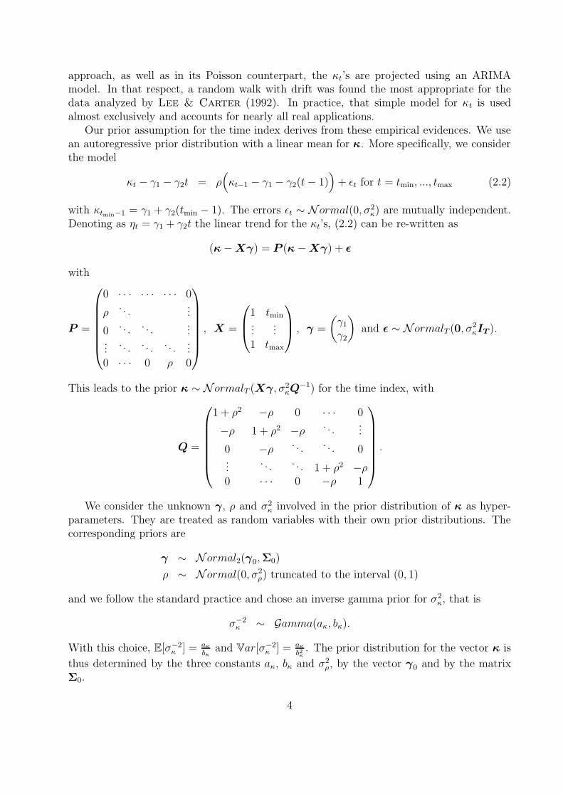
Our prior assumption for the time index derives from these empirical evidences. We usean autoregressive prior distribution with a linear mean for κ. More specifically, we considerthe model

κt − γ1 − γ2t = ρ(κt−1 − γ1 − γ2(t− 1)

)+ εt for t = tmin, ..., tmax (2.2)

with κtmin−1 = γ1 + γ2(tmin − 1). The errors εt ∼ N ormal(0, σ2κ) are mutually independent.

Denoting as ηt = γ1 + γ2t the linear trend for the κt’s, (2.2) can be re-written as

(κ−Xγ) = P (κ−Xγ) + ε

with

P =

0 · · · · · · · · · 0

ρ. . .

...

0. . .

. . ....

.... . .

. . .. . .

...0 · · · 0 ρ 0

, X =

1 tmin...

...1 tmax

, γ =

(γ1

γ2

)and ε ∼ N ormalT (0, σ2

κIT ).

This leads to the prior κ ∼ N ormalT (Xγ, σ2κQ−1) for the time index, with

Q =

1 + ρ2 −ρ 0 · · · 0

−ρ 1 + ρ2 −ρ . . ....

0 −ρ . . .. . . 0

.... . .

. . . 1 + ρ2 −ρ0 · · · 0 −ρ 1

.

We consider the unknown γ, ρ and σ2κ involved in the prior distribution of κ as hyper-

parameters. They are treated as random variables with their own prior distributions. Thecorresponding priors are

γ ∼ N ormal2(γ0,Σ0)

ρ ∼ N ormal(0, σ2ρ) truncated to the interval (0, 1)

and we follow the standard practice and chose an inverse gamma prior for σ2κ, that is

σ−2κ ∼ Gamma(aκ, bκ).

With this choice, E[σ−2κ ] = aκ

bκand Var[σ−2

κ ] = aκb2κ

. The prior distribution for the vector κ is

thus determined by the three constants aκ, bκ and σ2ρ, by the vector γ0 and by the matrix

Σ0.

4

2.3 Prior distribution for β

The parameters βx represent the age-specific pattern of mortality change: βx indicates thesensitivity of the logarithm of the force of mortality at age x to variations in the time index.The shape of the βx profile tells which rates decline rapidly and which slowly over time inresponse of change in κt.

The βx profile is usually much more erratic (see Brouhns et al. (2002a) for an illus-tration with Belgian data). Some of the βx’s are close to zero (especially for the ages aroundthe accident hump, for which mortality improvements are weak, as well as for older ages)while others are quite large (around birth for instance).

Our prior assumption for the βx’s is

β ∼ N ormalM(0, σ2βIM).

In words, we start from the assumption that no mortality improvements occur for the pop-ulation under study. The data will of course appropriately transform the prior distributionin case improvements do occur, as expected. Prior distributions for the hyperparameter σ2

β

is taken to be inverse gamma, to facilitate the computation. Specifically,

σ−2β ∼ Gamma(aβ, bβ)

for some constants aβ and bβ.

2.4 Prior distribution for α

For technical reasons, it is more convenient to deal with the transformed vector e = expα.The prior distribution for e is

ex ∼ Gamma(ax, bx)

for some constants ax and bx, with x = xmin, ..., xmax.

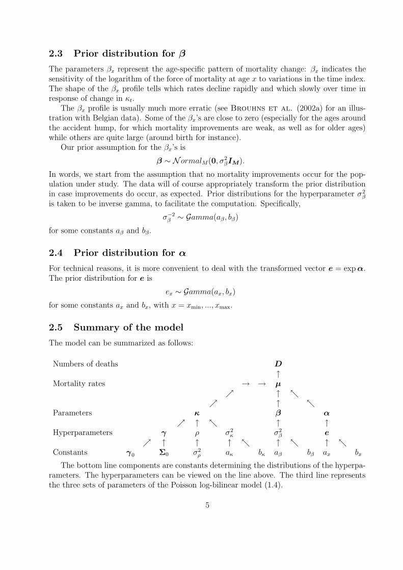
2.5 Summary of the model

The model can be summarized as follows:

Numbers of deaths D↑

Mortality rates → → µ↗ ↑ ↖

↗ ↑ ↖Parameters κ β α

↗ ↑ ↖ ↑ ↑Hyperparameters γ ρ σ2

κ σ2β e

↗ ↑ ↑ ↑ ↖ ↑ ↖ ↑ ↖Constants γ0 Σ0 σ2

ρ aκ bκ aβ bβ ax bx

The bottom line components are constants determining the distributions of the hyperpa-rameters. The hyperparameters can be viewed on the line above. The third line representsthe three sets of parameters of the Poisson log-bilinear model (1.4).

5

3 A posteriori distributions

3.1 MCMC approach

Inference about the αx’s, βx’s and κt’s is based on the posterior density of (α,β,κ) giventhe mortality statistics, that is on the density

p(α,β,κ|D) ∝ f(D|α,β,κ)p(α,β,κ). (3.1)

We make inference empirically by collecting many realizations from the posterior distributionp(α,β,κ|D). This is done by simulation: it is possible to set up a Markov chain whosestationary distribution is consistent with the posterior distribution (3.1). The Monte Carloapproach allows for inference based on sampling the posterior distribution of the parameters.A particularly attractive feature of this approach is the ease with which we can then explorethe uncertainty associated with the estimates and the forecasts.

In this section, we discuss implementation of the Bayes procedures via Markov ChainMonte Carlo (MCMC). In particular, we use the Gibbs sampler and Metropolis-Hastingsalgorithm to generate samples from the posterior (3.1).

Let us now describe the MCMC procedure more formally. Consider a random vector Zwith joint probability density function h. In a Bayesian context, some of the components ofZare model parameters, while others may represent unobserved past or future data. Supposeh is so complicated and analytically intractable that it does not permit independent randomdraws. In this case a MCMC simulation method may be used.

The main idea behind a MCMC method is to simulate realizations from a Markov chainwhich has h as its stationary distribution. The resulting random draws Z (1),Z(2), . . . are nolonger independent, but under mild regularity conditions (as described in the Appendix ofSmith & Roberts (1993), for example), the value of Z (t) tends in distribution to that ofa random draw from h as t becomes moderately large.

Determining how long a MCMC simulation should be run is a function of the particularapplication. Usually, several tens of thousands of iterations are enough. In any case, thefirst portion of the simulated Markov chain is discarded in order to reduce the effect of thestarting values. An ad hoc but useful test of convergence is obtained by running severalsimulations in parallel, with different starting values, and then comparing the results: thenumber of iterations must be increased if the results look rather different.

3.2 Metropolis-Hastings sampling for the time index vector κ

Metropolis-Hastings algorithms produce Markov chains whose stationary distribution is pre-cisely (3.1) from which the sample have to be drawn. These algorithms are based on aMarkov chain whose dependence on the predecessor is split into two parts: a proposal andan acceptance of the proposal. The proposals suggest an arbitrary next step in the trajectoryof the chain and the acceptance makes sure the appropriate limiting direction is maintainedby rejecting unwanted moves of the chain.

Let us denote as

κ−t = (κtmin, ..., κt−1, κt+1, ..., κtmax)′

6

the time index vector κ without its t-th component. Denoting as

Dt = (Dxmint, . . . , Dxmaxt)′,

the vector of the Dxt’s, we define in the same way

D−t = (Dtmin, ...,Dt−1,Dt+1, ...,Dtmax)′

as the matrix of the death counts Dxt without the column corresponding to calendar year t.Now, each κ update is realized elementwise according to Metropolis-Hastings sampling.

Specifically we look for the conditional probability density function f(κt|κ−t,α,β,D, σ2κ, σ

2β,γ, ρ)

that is, the density of κt given all other parameters and hyper-parameters, as well as datapoints. Some manipulations yield

f(κt|κ−t,α,β,D, σ2κ, σ

2β,γ, ρ)

=f(κ,α,β,D, σ2

κ, σ2β,γ, ρ)

f(κ−t,α,β,D, σ2κ, σ

2β,γ, ρ)

=f(κtmax ,Dtmax |κ−tmax ,D−tmax ,α,β, σ

2κ, σ

2β,γ, ρ)f(κ−tmax ,D−tmax ,α,β, σ

2κ, σ

2β,γ, ρ)

f(κ−t,D,α,β, σ2κ, σ

2β,γ, ρ)

.

Iterating this formula gives

f(κt|κ−t,α,β,D, σ2κ, σ

2β,γ, ρ)

=f(α,β, σ2

κ, σ2β,γ, ρ)

f(κ−t,D,α,β, σ2κ, σ

2β,γ, ρ)

f(κtmin,Dtmin

|α,β, σ2κ, σ

2β,γ, ρ)

tmax∏

s=tmin+1

f(κs,Ds|κtmin, ..., κs−1,Dtmin

, ...,Ds−1,α,β, σ2κ, σ

2β,γ, ρ)

∝ f(κtmin,Dtmin

|α,β, σ2κ, σ

2β,γ, ρ)

tmax∏

s=tmin+1

f(κs,Ds|κtmin, ..., κs−1,Dtmin

, ...,Ds−1,α,β, σ2κ, σ

2β,γ, ρ).

Remember that the random vectors Ds are mutually independent given κ,α,β, σ2κ, σ

2β,γ, ρ.

Moreover, their conditional distribution only depends on (κs,α,β). This allows us to write

f(κs,Ds|κtmin, ..., κs−1,Dtmin

, ...,Ds−1,α,β, σ2κ, σ

2β,γ, ρ)

= f(Ds|κtmin, ..., κs−1, κs,Dtmin

, ...,Ds−1,α,β, σ2κ, σ

2β,γ, ρ)

f(κs|κtmin, ..., κs−1,Dtmin

, ...,Ds−1,α,β, σ2κ, σ

2β,γ, ρ)

= f(Ds|κs,α,β)f(κs|κtmin, ..., κs−1,Dtmin

, ...,Ds−1,α,β, σ2κ, σ

2β,γ, ρ)

= f(Ds|κs,α,β)f(κs|κs−1,γ, σ2κ, ρ).

Finally we find the following expression for the conditional density of κt:

f(κt|κ−t,α,β,D, σ2κ, σ

2β,γ, ρ)

∝ f(Dtmin|κtmin

,α,β)f(κtmin|γ, σ2

κ)

tmax∏

s=tmin+1

f(Ds|κs,α,β)f(κs|κs−1,γ, σ2κ, ρ).

Let us now consider three cases:

7

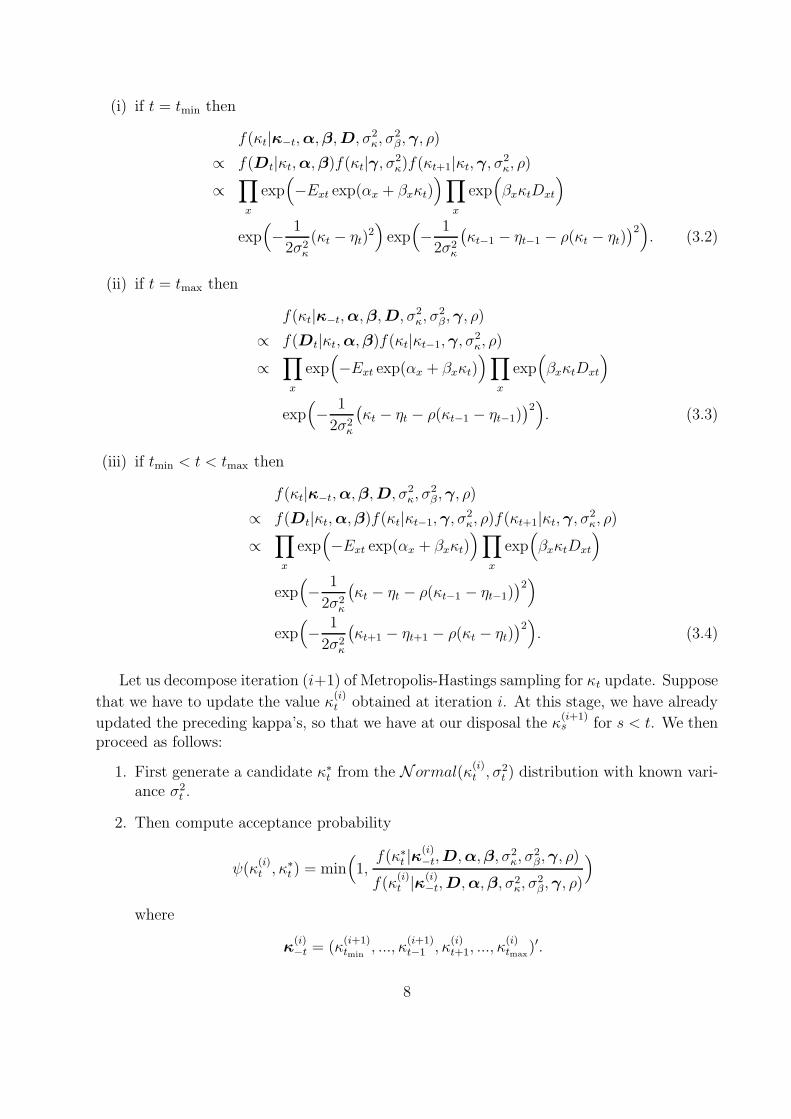
(i) if t = tmin then

f(κt|κ−t,α,β,D, σ2κ, σ

2β,γ, ρ)

∝ f(Dt|κt,α,β)f(κt|γ, σ2κ)f(κt+1|κt,γ, σ2

κ, ρ)

∝∏

x

exp(−Ext exp(αx + βxκt)

)∏

x

exp(βxκtDxt

)

exp(− 1

2σ2κ

(κt − ηt)2)

exp(− 1

2σ2κ

(κt−1 − ηt−1 − ρ(κt − ηt)

)2). (3.2)

(ii) if t = tmax then

f(κt|κ−t,α,β,D, σ2κ, σ

2β,γ, ρ)

∝ f(Dt|κt,α,β)f(κt|κt−1,γ, σ2κ, ρ)

∝∏

x

exp(−Ext exp(αx + βxκt)

)∏

x

exp(βxκtDxt

)

exp(− 1

2σ2κ

(κt − ηt − ρ(κt−1 − ηt−1)

)2). (3.3)

(iii) if tmin < t < tmax then

f(κt|κ−t,α,β,D, σ2κ, σ

2β,γ, ρ)

∝ f(Dt|κt,α,β)f(κt|κt−1,γ, σ2κ, ρ)f(κt+1|κt,γ, σ2

κ, ρ)

∝∏

x

exp(−Ext exp(αx + βxκt)

)∏

x

exp(βxκtDxt

)

exp(− 1

2σ2κ

(κt − ηt − ρ(κt−1 − ηt−1)

)2)

exp(− 1

2σ2κ

(κt+1 − ηt+1 − ρ(κt − ηt)

)2). (3.4)

Let us decompose iteration (i+1) of Metropolis-Hastings sampling for κt update. Suppose

that we have to update the value κ(i)t obtained at iteration i. At this stage, we have already

updated the preceding kappa’s, so that we have at our disposal the κ(i+1)s for s < t. We then

proceed as follows:

1. First generate a candidate κ∗t from the N ormal(κ(i)t , σ

2t ) distribution with known vari-

ance σ2t .

2. Then compute acceptance probability

ψ(κ(i)t , κ

∗t ) = min

(1,f(κ∗t |κ(i)

−t,D,α,β, σ2κ, σ

2β,γ, ρ)

f(κ(i)t |κ(i)

−t,D,α,β, σ2κ, σ

2β,γ, ρ)

)

where

κ(i)−t = (κ

(i+1)tmin

, ..., κ(i+1)t−1 , κ

(i)t+1, ..., κ

(i)tmax

)′.

8

3. Afterwards generate a realization u from the Uniform(0, 1) distribution. If u ≤ψ(κ

(i)t , κ

∗t ) then the candidate is kept and κ

(i+1)t = κ∗t . On the contrary, if u > ψ(κ

(i)t , κ

∗t )

then the candidate is rejected and the Markov chain does not move (κ(i+1)t = κ

(i)t ).

4. Finally we have to transform

κ(i+1) =(κ

(i+1)tmin

, . . . , κ(i+1)t , κ

(i)t+1, . . . , κ

(i)tmax

)′

and α(i) in order to fulfill the constraints (1.3). To this end, we use the followingformulas:

κ(i+1) ← κ(i+1) − κα(i) ← α(i) + β(i)κ

where

κ =1

T

(∑

s≤tκ(i+1)s +

∑

s>t

κ(i)s

).

Remark that the choice of parameter σ2t is free but not neglectable. It directly influences

acceptance rate of the proposals: a large variance will reduce the chance for the candidateto be kept and for the chain to move to another state. In practice we want the acceptationprobability to be in the interval [20%, 50%]. Therefore, a trial and error method is usedto select σ2

t . Starting from some initial value, we compute the acceptation probability (onabout one hundred iterations, say). If it is too small, we have to increase the variance σ2

t

(make it double, say). On the contrary, if more than half the candidates are kept, we reducethe value of σ2

t .

3.3 Metropolis-Hastings sampling for β

The β update is quite similar to the κ one. Let us define

β−x = (βxmin, ..., βx−1, βx+1, ..., βxmax)′

and in the same way

D−x = (Dxmin, ...,Dx−1,Dx+1, ...,Dxmax)′

9

where Dx is the (x − xmin + 1)-th row of D. With the same developments as in previoussection we find

f(βx|β−x,α,κ,D, σ2κ, σ

2β,γ, ρ)

∝xmax∏

y=xmin

f(βy,Dy|βxmin, ..., βy−1,Dxmin

, ...,Dy−1,α,κ, σ2κ, σ

2β,γ, ρ)

∝xmax∏

y=xmin

f(Dy|βxmin, ..., βy−1, βy,Dxmin

, ...,Dy−1,α,κ, σ2κ, σ

2β,γ, ρ)

xmax∏

y=xmin

f(βy|βxmin, ..., βy−1,Dxmin

, ...,Dy−1,α,κ, σ2κ, σ

2β,γ, ρ)

∝xmax∏

y=xmin

f(Dy|βy,α,κ)f(βy)

∝ f(Dx|βx,α,κ)f(βx)

∝∏

t

exp(−Ext exp(αx + βxκt)

)∏

t

exp(βxκtDxt

)exp(− 1

2σ2β

β2x

). (3.5)

Now we can decompose iteration (i+ 1) of Metropolis-Hastings sampling for βx update.

Suppose the parameter is estimated at iteration i by β(i)x and we have estimations β

(i+1)y for

y < x. We then proceed as follows:

1. Select a candidate β∗x from the N ormal(β(i)x , σ2

x) distribution with known variance σ2x.

2. Compute the acceptance probability

ψ(β(i)x , β

∗x) = min

(1,f(β∗x|β(i)

−x,D,α,κ, σ2κ, σ

2β,γ, ρ)

f(β(i)x |β(i)

−x,D,α,κ, σ2κ, σ

2β,γ, ρ)

)

where

β(i)−x = (β(i+1)

xmin, ..., β

(i+1)x−1 , β

(i)x+1, ..., β

(i)xmax

)′.

3. Afterwards generate a realization u from the Uniform(0, 1) distribution. If u ≤ψ(β

(i)x , β∗x), the candidate is kept and β

(i+1)x = β∗x. On the contrary, if u > ψ(β

(i)x , β∗x),

the candidate is rejected and the Markov chain does not move (β(i+1)x = β

(i)x ).

4. Finally we have to transform vectors

β(i+1) =(β(i+1)xmin

, . . . , β(i+1)x , β

(i)x+1, . . . , β

(i)xmax

)′

and κ(i+1) in order to fulfill constraints (1.3):

β(i+1) ← β(i+1)

β•κ(i+1) ← κ(i+1)β•

10

where

β• =∑

y≤xβ(i+1)y +

∑

y>x

β(i)y .

As for κ update, the variance σ2x must be adjusted in order to have acceptance probabil-

ities between 20% and 50%.

3.4 Gibbs sampling for α

Another standard approach which produces a Markov chain whose stationary distributionis consistent with the posterior distribution (3.1) is based on a variant of the Metropolisalgorithm called the Gibbs sampler. It will enable us to exploit conditional densities to obtainrealizations from the posterior density. The Gibbs sampler requires that the unknown modelparameters are first assigned arbitrary values. Then an iterative sampling process takes place.At each iteration, the Gibbs sampler visits each unknown parameter in turn, and generatesa random value from its full conditional distribution, conditional upon current values of allother parameters and upon the data. Then, each iteration yields a sample realization of thecomplete set of unknown parameters in the model. The generated realizations converge indistribution to the joint posterior distribution of the unknwown parameters.

Let us consider the likelihood function (2.1) as function of the vector e only:

L(e,β,κ) ∝∏

x

∏

t

exp(−Ext exp(αx + βxκt) +Dxt(αx + βxκt)

)

∝∏

x

exp(−cxex)eDx•x

withcx =

∑

t

Ext exp(βxκt) and Dx• =∑

t

Dxt.

To draw random samples from the posterior density, we use the Gibbs sampling algorithm.The essence of the Gibbs sampler lies in breaking a complicated joint probability densityinto a set of full conditional densities, and sampling one variable at a time, conditional onthe values of the others.

For x = xmin, ..., xmax, we can write

f(ex|β,κ,D, σ2κ, σ

2β,γ, ρ) = f(ex|β,κ,D)

∝ f(ex,β,κ,D)f(ex)

∝ exp(−cxex)eDx•x eax−1x exp(−bxex)

∝ exp(−(bx + cx)ex

)eax+Dx•−1x

so that the distribution of ex given β,κ,D, σ2κ, σ

2β,γ, ρ is still gamma with updated param-

eters, that is,

(ex|β,κ,D, σ2κ, σ

2β,γ, ρ) ∼ Gamma(ax +Dx•, bx + cx). (3.6)

Realizations of ex given β,κ,D, σ2κ, σ

2β,γ, ρ are thus easily generated.

11

3.5 Gibbs sampling for ρ

From conditional distribution definition we have

f(ρ|α,β,κ,D, σ2κ, σ

2β,γ) =

f(ρ,α,β,κ,D, σ2κ, σ

2β,γ)

f(α,β,κ,D, σ2κ, σ

2β,γ)

∝ f(D|ρ,α,β,κ, σ2κ, σ

2β,γ)f(ρ,α,β,κ, σ2

κ, σ2β,γ)

= f(D|α,β,κ)f(κ, ρ|α,β, σ2κ, σ

2β,γ)f(α,β, σ2

κ, σ2β,γ)

∝ f(κ, ρ)

= f(κ|ρ)f(ρ).

The conditional density of κ given ρ is given by

f(κ|ρ) =∏

t

f(κt|κt−1, ρ) ∝ exp(− 1

2σ2κ

(aρρ2 − 2bρρ)

)

withaρ =

∑

t

(κt−1 − ηt−1)2 and bρ =∑

t

(κt − ηt)(κt−1 − ηt−1)

and the convention κtmin−1 = ηtmin−1. Therefore,

f(ρ|α,β,κ,D, σ2κ, σ

2β,γ) ∝ exp

(− 1

2σ2κ

(aρρ2 − 2bρρ)

)exp(− 1

2σ2ρ

ρ2)

∝ exp(− 1

2σ2ρ∗ (ρ− µ∗ρ)2

)

with

µ∗ρ =bρ

aρ + σ2κ

σ2ρ

and σ2ρ∗

=σ2κ

aρ + σ2κ

σ2ρ

.

The distribution of ρ given α,β,κ,D, σ2κ, σ

2β,γ can then be written as

(ρ|α,β,κ,D, σ2κ, σ

2β,γ) ∼ N ormal(µ∗ρ, σ2

ρ∗) truncated to (−1, 1). (3.7)

Simulation from (3.7) is easy.

3.6 Gibbs sampling for σ2κ

By using the same principles as previously we find

f(σ2κ|α,β,κ,D, σ2

β,γ, ρ) ∝ f(κ|σ2κ)f(σ2

κ).

Since

f(κ|σ2κ) =

1

2πσ2κ

exp(− 1

2σ2κ

∑

t

(κt − ηt − ρ(κt−1 − ηt−1)

)2)

12

and the prior distribution of σ−2κ is Gamma(aκ, bκ), we find

f(σ2κ|α,β,κ,D, σ2

β,γ, ρ) ∝ σκ−2(aκ+1+T

2) exp

(− 1

σ2κ

(bκ +

1

2

∑

t

(κt − ηt − ρ(κt−1 − ηt−1)

)2))

with κtmin−1 = ηtmin−1. The distribution of σ−2κ given α,β,κ,D, σ2

β,γ, ρ is then given by

(σ−2κ |α,β,κ,D, σ2

β,γ, ρ) ∼ Gamma(aκ +

T

2, bκ +

1

2

∑

t

(κt − ηt − ρ(κt−1 − ηt−1)

)2). (3.8)

3.7 Gibbs sampling for σ2β

Applying the same reasoning as before, we find

f(σ2β|α,β,κ,D, σ2

κ,γ, ρ) ∝ f(β|σ2β)f(σ2

β)

∝ σβ−2(aβ+1+M

2) exp

(− 1

σ2β

(bβ +

1

2β′β

)).

The distribution of σ−2β given α,β,κ,D, σ2

κ,γ, ρ is then given by

(σ−2β |α,β,κ,D, σ2

κ,γ, ρ) ∼ Gamma(aβ +M

2, bβ +

1

2β′β). (3.9)

3.8 Gibbs sampling for γ

As previously we have

f(γ|κ, σ2κ, σ

2β, ρ) ∝ f(κ|γ, ρ, σ2

κ)f(γ).

Because γ is a priori distributed according to N ormal2(γ0,Σ0), we find

f(γ|κ, σ2κ, σ

2β, ρ) ∝ exp

(− 1

2σ2κ

(κ−Xγ)′Q(κ−Xγ))

exp(−1

2(γ − γ0)′Σ−1

0 (γ − γ0))

∝ exp(− 1

2σ2κ

(γ − γ∗)′Σ∗−1(γ − γ∗))

withΣ∗ = (X ′QX + σ2

κΣ−10 )−1 and γ∗ = Σ∗(X ′Qκ+ σ2

κΣ−10 γ0).

Thus the distribution of γ given κ, σ2κ, σ

2β, ρ is

(γ|κ, σ2κ, σ

2β, ρ) ∼ N ormal2(γ∗, σ2

κΣ∗). (3.10)

13

4 Numerical illustration

4.1 Data set

Our data are about French male population aged 0 to 89 between 1950 and 2000. Thedata related to calendar years 1950 to 1997 come from INED (Institut National d’EtudesDemographiques based in Paris, France). Those related to calendar years 1998, 1999 and2000 have been obtained from INSEE (Institut National de la Statistique et des EtudesEconomiques based in Paris, France). The following information is available: the numbersLxt of people aged x on January 1 of year t (for x between 0 and 89), and the numbersDxt of people aged x dying during year t. The exposure-to-risk Ext is then computed underassumption (1.1).

4.2 Initialization and choice of prior distributions for the hyper-parameters

As seen in the previous section, we work with three vectors of parameters (α, β and κ) andwith five hyperparameters (ρ, σ2

κ, σ2β and the two components of γ). We also have to fix the

constants aκ, bκ, aβ, bβ, σ2ρ, the M components ax, the M components bx, the vector γ0 and

the matrix Σ0 involved in the distribution of the hyperparameters.The choices for the constants determining the distributions of the hyperparameters are

made in an empirical Bayes approach. In empirical Bayes, hyperparameters from the lastlevel of a hierarchical model are estimated rather than chosen a priori. Although this proce-dure might seem better because it lets the data decide about reasonable values for obscurehyperparameters, many theoretical arguments have been levelled against it. Despite theinferential problems, this procedure is often used (namely because using the data in this wayturns out to be equivalent to making the prior indifferent to certain chosen parameters; seee.g. Carlin & Louis (2000)).

Specifically, we first compute the frequentist estimates of α, β and κ by maximizing thelikelihood (2.1), as described in Brouhns et al. (2002a,b). Because of the presence ofthe bilinear term βxκt, it is not possible to estimate the proposed model with commercialstatistical packages that implement Poisson regression. A uni-dimensional or elementaryNewton method is used instead as proposed by Goodman (1979) for estimating log-linearmodels with bilinear terms. The estimators of α, β and κ obtained in this way are furtherreferred to as Goodman estimates.

We take for γ0 the estimated parameters of a linear regression of κ on calendar time.Then, Σ0 is taken to be the estimated covariance matrix of these estimates. Afterwards, ρand σ2

κ can be initialized by fitting an AR(1) model on (κ− γ0X). Finally σ2β is initialized

to be the empirical variance of the Goodman βx’s.When the model (1.2) is fitted by ordinary least-squares, the fitted values of αx exactly

equal the average of ln µx(t) over time t so that expαx is the general shape of the mortalityschedule. Also, in the Poisson log-bilinear model, the fitted expαx mimick the observedaverage of the µx(t)’s. In order to obtain an uninformative prior distribution (i.e. with largevariance), we have to choose a small bx, 0.001 say. Afterwards, ax can be choosen equal tobx exp αx (so that E[ex] = exp αx).

14

In the same way, if σ−2β ∼ Gamma(aβ, bβ), then E[σ2

β] =bβ

aβ−1for aβ > 1 and Var[σ2

β] =b2β

(aβ−1)2(aβ−2)for aβ > 2. So constants aβ and bβ control prior mean and variance of σ2

β.

Taking aβ near to (but greater than) 2 will give a huge variance. So we find bβ = (aβ− 1)σ2β.

The same argument can be used for aκ and bκ. We use aβ = aκ = 2.1 for the application.Finally the initial value of σ2

ρ does not seem to be very influential since ρ is restricted tointerval (0, 1). We choose σ2

ρ = 1.It is worth to mention that other constants have also been used. Typically, we have

increased the a priori variance of parameters and hyperparameters. These more diffuse priorchoices were based on smaller values of bx (from 0.001 to 0.00001), values of aβ closer to2 (from 2.1 to 2.00001), and “greater” matrix Σ0 (up to 10 times the initial matrix). Theresults were similar to those obtained with the initial values deduced from the empiricalBayes approach.

Instead of basing the prior choices of the parameters on the Goodman’s estimations of α,β and κ, we also used the Lee-Carter estimates to fix the constants and init hyperparametersand parameters involved in the model (in an empirical Bayes setting). Again, the resultsobtained in this way were almost identical to those obtained with the Goodman’s estimations.

4.3 Convergence diagnostics

In practice, we typically run the Gibbs sampler for an initial period of a few thousandscycles and then collect information from several further thousands of cycles (of which westore every 10th for the subsequent construction of approximate interval estimates). Theposterior means are estimated by the corresponding sample means. Here, 20 000 iterationsare computed. The first 10 000 iterations are considered as the burn-in period. The last 10000 iterations are used for estimation of the posterior distribution.

A sample from the distribution of interest (the posterior distribution of the parameterin our example) is only attained with MCMC when the number of iterations of the chainapproaches infinity. This is of course impossible in practice and a value obtained at asufficiently large iteration is taken instead. This raises the question of how large this iterationshould be.

Some informal checks of convergence based on graphical techniques are commonly used.Several chains can be run in parallel with different initial states or a single chain is screenedfor exhibiting the same qualitative behavior through iterations (often after a transient initialperiod). More formal diagnostics are developed in Cowles & Carlin (1996) and Brooks& Roberts (1998).

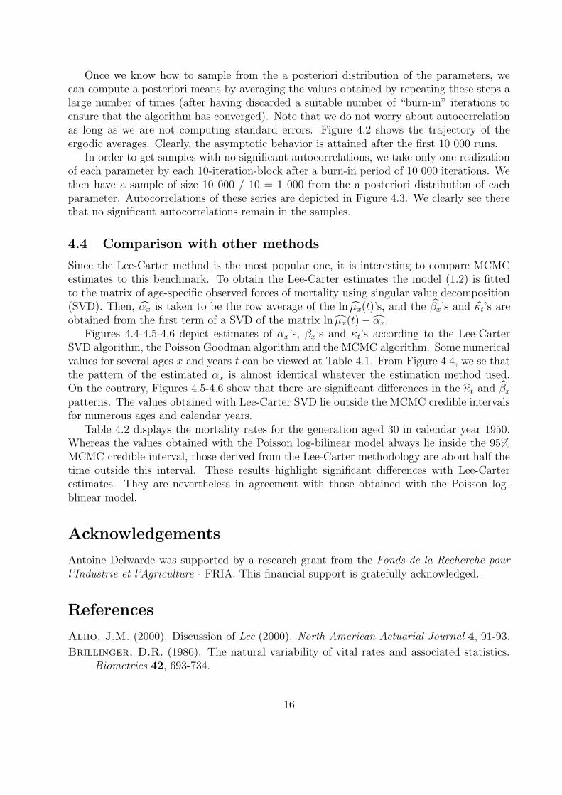
Figure 4.1 gives the selected σ2t and σ2

x and corresponding acceptation probabilities.These variances are selected by a trial an error method. Algorithm starts with σ2

x = σ2t = 1

for all x and t, and a first 100-iteration-pilot run is computed. Variance σ2x (or σ2

t ) ismade double if the corresponding acceptation probability is below 20%; it is divided by 2if corresponding acceptation probability is greater than 50%. A second 100-iteration-pilotrun is then computed and variances σ2

x and σ2t are moving as previously. The algorithm

stops when rates for each age x and each year t are between 20% and 50%. We observelarger variances σ2

x where mortality is very specific, i.e. between ages 0 and 40 (new borns,accidental hump). In the same way variance σ2

t grows with year t.

15

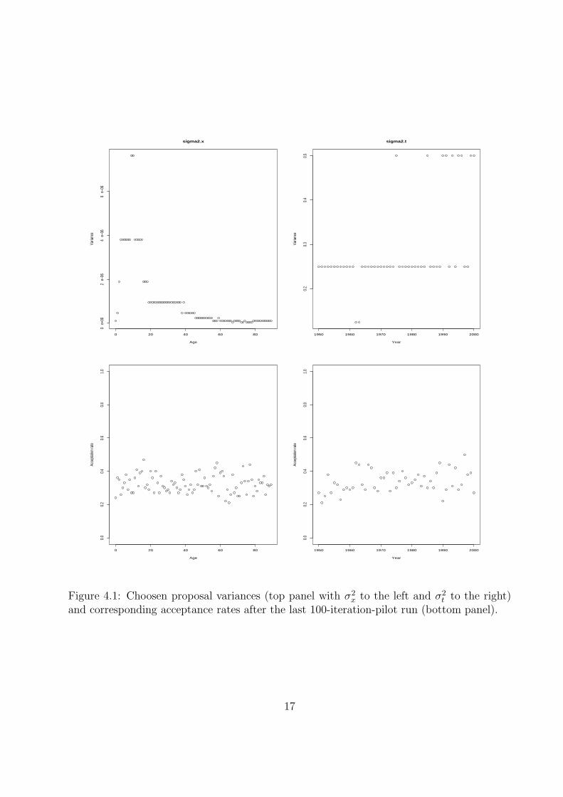
Once we know how to sample from the a posteriori distribution of the parameters, wecan compute a posteriori means by averaging the values obtained by repeating these steps alarge number of times (after having discarded a suitable number of “burn-in” iterations toensure that the algorithm has converged). Note that we do not worry about autocorrelationas long as we are not computing standard errors. Figure 4.2 shows the trajectory of theergodic averages. Clearly, the asymptotic behavior is attained after the first 10 000 runs.

In order to get samples with no significant autocorrelations, we take only one realizationof each parameter by each 10-iteration-block after a burn-in period of 10 000 iterations. Wethen have a sample of size 10 000 / 10 = 1 000 from the a posteriori distribution of eachparameter. Autocorrelations of these series are depicted in Figure 4.3. We clearly see therethat no significant autocorrelations remain in the samples.

4.4 Comparison with other methods

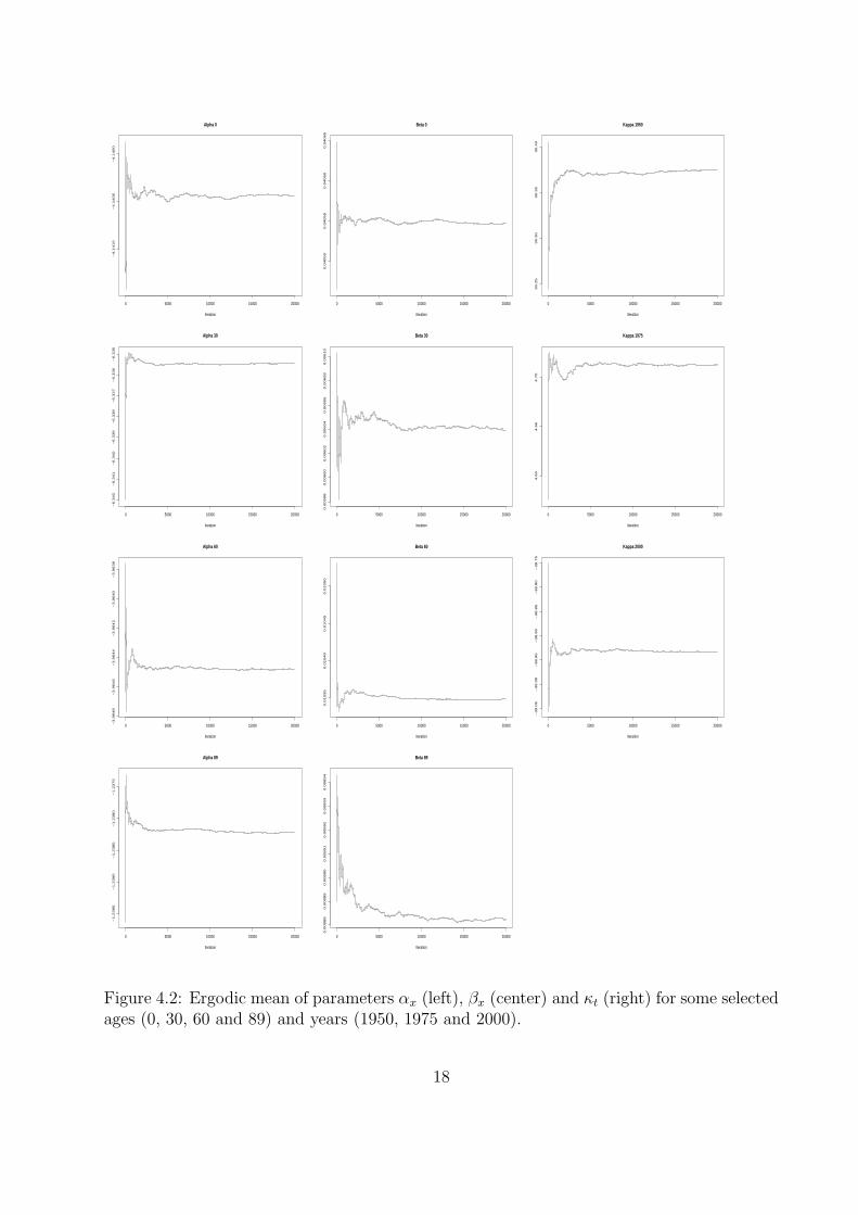
Since the Lee-Carter method is the most popular one, it is interesting to compare MCMCestimates to this benchmark. To obtain the Lee-Carter estimates the model (1.2) is fittedto the matrix of age-specific observed forces of mortality using singular value decomposition(SVD). Then, αx is taken to be the row average of the ln µx(t)’s, and the βx’s and κt’s areobtained from the first term of a SVD of the matrix ln µx(t)− αx.

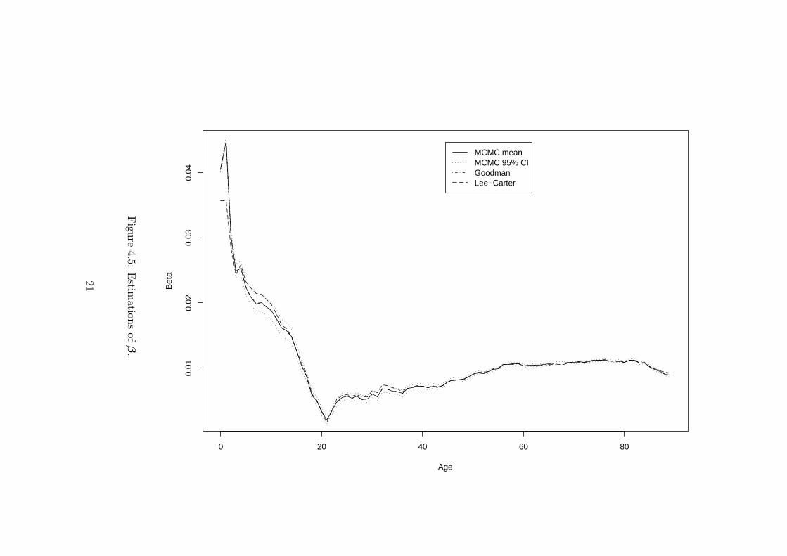
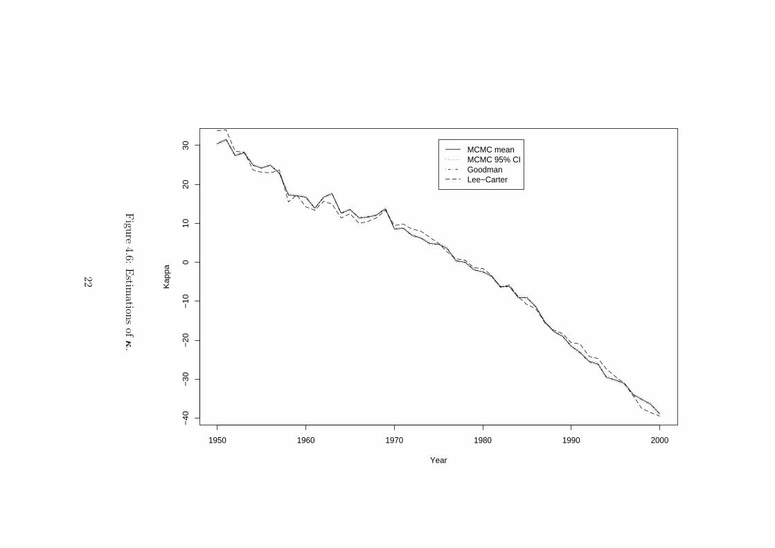
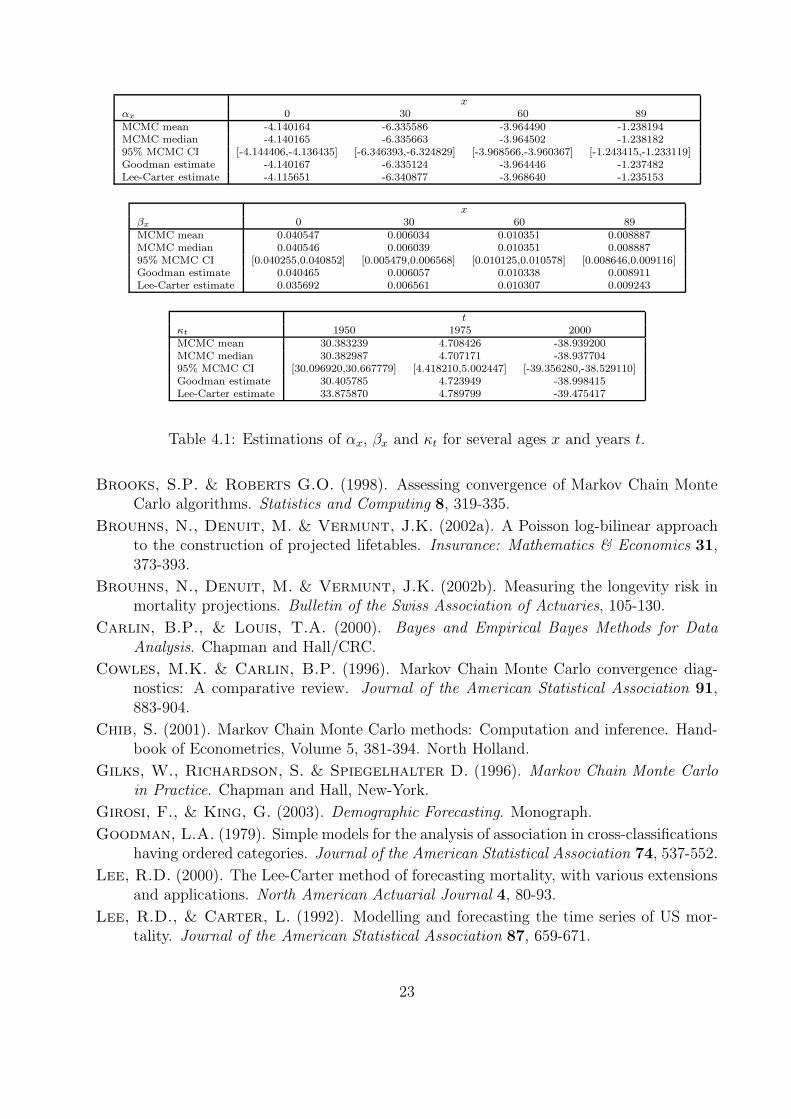
Figures 4.4-4.5-4.6 depict estimates of αx’s, βx’s and κt’s according to the Lee-CarterSVD algorithm, the Poisson Goodman algorithm and the MCMC algorithm. Some numericalvalues for several ages x and years t can be viewed at Table 4.1. From Figure 4.4, we se thatthe pattern of the estimated αx is almost identical whatever the estimation method used.On the contrary, Figures 4.5-4.6 show that there are significant differences in the κt and βxpatterns. The values obtained with Lee-Carter SVD lie outside the MCMC credible intervalsfor numerous ages and calendar years.

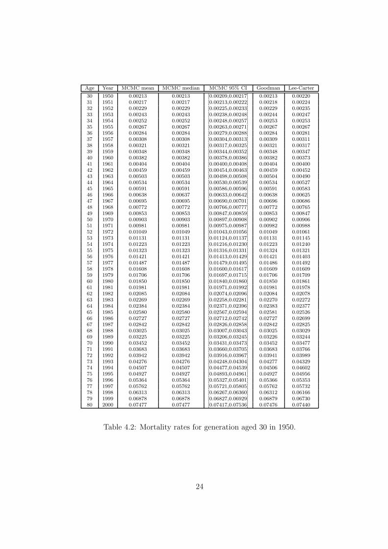
Table 4.2 displays the mortality rates for the generation aged 30 in calendar year 1950.Whereas the values obtained with the Poisson log-bilinear model always lie inside the 95%MCMC credible interval, those derived from the Lee-Carter methodology are about half thetime outside this interval. These results highlight significant differences with Lee-Carterestimates. They are nevertheless in agreement with those obtained with the Poisson log-blinear model.

Acknowledgements

Antoine Delwarde was supported by a research grant from the Fonds de la Recherche pourl’Industrie et l’Agriculture - FRIA. This financial support is gratefully acknowledged.

References

Alho, J.M. (2000). Discussion of Lee (2000). North American Actuarial Journal 4, 91-93.

Brillinger, D.R. (1986). The natural variability of vital rates and associated statistics.Biometrics 42, 693-734.

16

0 20 40 60 80

0 e

+00

2 e

−06

4 e

−06

6 e

−06

sigma2.x

Age

Varia

nce

1950 1960 1970 1980 1990 2000

0.2

0.3

0.4

0.5

sigma2.t

Year

Varia

nce

0 20 40 60 80

0.0

0.2

0.4

0.6

0.8

1.0

Age

Acce

ptat

ion

rate

1950 1960 1970 1980 1990 2000

0.0

0.2

0.4

0.6

0.8

1.0

Year

Acce

ptat

ion

rate

Figure 4.1: Choosen proposal variances (top panel with σ2x to the left and σ2

t to the right)and corresponding acceptance rates after the last 100-iteration-pilot run (bottom panel).

17

0 5000 10000 15000 20000

−4

.14

10

−4

.14

05

−4

.14

00

Alpha 0

Iteration

0 5000 10000 15000 20000

0.0

4050

0.0

4055

0.0

4060

0.0

4065

Beta 0

Iteration

0 5000 10000 15000 20000

30.2

530.3

030.3

530.4

0

Kappa 1950

Iteration

0 5000 10000 15000 20000

−6

.34

2−

6.3

41

−6

.34

0−

6.3

39

−6

.33

8−

6.3

37

−6

.33

6−

6.3

35

Alpha 30

Iteration

0 5000 10000 15000 20000

0.0

0598

0.0

0600

0.0

0602

0.0

0604

0.0

0606

0.0

0608

0.0

0610

Beta 30

Iteration

0 5000 10000 15000 20000

4.6

04.6

54.7

0

Kappa 1975

Iteration

0 5000 10000 15000 20000−3

.96

48

−3

.96

46

−3

.96

44

−3

.96

42

−3

.96

40

−3

.96

38

Alpha 60

Iteration

0 5000 10000 15000 20000

0.0

1035

0.0

1040

0.0

1045

0.0

1050

Beta 60

Iteration

0 5000 10000 15000 20000

−3

9.0

5−

39

.00

−3

8.9

5−

38

.90

−3

8.8

5−

38

.80

−3

8.7

5

Kappa 2000

Iteration

0 5000 10000 15000 20000

−1

.23

95

−1

.23

90

−1

.23

85

−1

.23

80

−1

.23

75

Alpha 89

Iteration

0 5000 10000 15000 20000

0.0

0888

0.0

0889

0.0

0890

0.0

0891

0.0

0892

0.0

0893

0.0

0894

Beta 89

Iteration

Figure 4.2: Ergodic mean of parameters αx (left), βx (center) and κt (right) for some selectedages (0, 30, 60 and 89) and years (1950, 1975 and 2000).

18

0 5 10 15 20 25 30

0.0

0.2

0.4

0.6

0.8

1.0

Lag

Alpha 0

0 5 10 15 20 25 30

0.0

0.2

0.4

0.6

0.8

1.0

Lag

Beta 0

0 5 10 15 20 25 30

0.0

0.2

0.4

0.6

0.8

1.0

Lag

Kappa 1950

0 5 10 15 20 25 30

0.0

0.2

0.4

0.6

0.8

1.0

Lag

Alpha 30

0 5 10 15 20 25 30

0.0

0.2

0.4

0.6

0.8

1.0

Lag

Beta 30

0 5 10 15 20 25 30

0.0

0.2

0.4

0.6

0.8

1.0

Lag

Kappa 1975

0 5 10 15 20 25 30

0.0

0.2

0.4

0.6

0.8

1.0

Lag

Alpha 60

0 5 10 15 20 25 30

0.0

0.2

0.4

0.6

0.8

1.0

Lag

Beta 60

0 5 10 15 20 25 30

0.0

0.2

0.4

0.6

0.8

1.0

Lag

Kappa 2000

0 5 10 15 20 25 30

0.0

0.2

0.4

0.6

0.8

1.0

Lag

Alpha 89

0 5 10 15 20 25 30

0.0

0.2

0.4

0.6

0.8

1.0

Lag

Beta 89

Figure 4.3: Autocorrelations of parameters αx (left), βx (center) and κt (right) for someselected ages (0, 30, 60 and 89) and years (1950, 1975 and 2000) based on 1000 recordediterations after a burn-in period of 10 000 iterations.

19

0 20 40 60 80

−8

−7

−6

−5

−4

−3

−2

−1

Age

Alp

ha

MCMC meanMCMC 95% CIGoodmanLee−Carter

Figu

re4.4:

Estim

ations

ofα

.

20

0 20 40 60 80

0.0

10

.02

0.0

30

.04

Age

Be

ta

MCMC meanMCMC 95% CIGoodmanLee−Carter

Figu

re4.5:

Estim

ations

ofβ

.

21

1950 1960 1970 1980 1990 2000

−4

0−

30

−2

0−

10

01

02

03

0

Year

Ka

pp

a

MCMC meanMCMC 95% CIGoodmanLee−Carter

Figu

re4.6:

Estim

ations

ofκ

.

22

xαx 0 30 60 89MCMC mean -4.140164 -6.335586 -3.964490 -1.238194MCMC median -4.140165 -6.335663 -3.964502 -1.23818295% MCMC CI [-4.144406,-4.136435] [-6.346393,-6.324829] [-3.968566,-3.960367] [-1.243415,-1.233119]Goodman estimate -4.140167 -6.335124 -3.964446 -1.237482Lee-Carter estimate -4.115651 -6.340877 -3.968640 -1.235153

xβx 0 30 60 89MCMC mean 0.040547 0.006034 0.010351 0.008887MCMC median 0.040546 0.006039 0.010351 0.00888795% MCMC CI [0.040255,0.040852] [0.005479,0.006568] [0.010125,0.010578] [0.008646,0.009116]Goodman estimate 0.040465 0.006057 0.010338 0.008911Lee-Carter estimate 0.035692 0.006561 0.010307 0.009243

tκt 1950 1975 2000MCMC mean 30.383239 4.708426 -38.939200MCMC median 30.382987 4.707171 -38.93770495% MCMC CI [30.096920,30.667779] [4.418210,5.002447] [-39.356280,-38.529110]Goodman estimate 30.405785 4.723949 -38.998415Lee-Carter estimate 33.875870 4.789799 -39.475417

Table 4.1: Estimations of αx, βx and κt for several ages x and years t.

Brooks, S.P. & Roberts G.O. (1998). Assessing convergence of Markov Chain MonteCarlo algorithms. Statistics and Computing 8, 319-335.

Brouhns, N., Denuit, M. & Vermunt, J.K. (2002a). A Poisson log-bilinear approachto the construction of projected lifetables. Insurance: Mathematics & Economics 31,373-393.

Brouhns, N., Denuit, M. & Vermunt, J.K. (2002b). Measuring the longevity risk inmortality projections. Bulletin of the Swiss Association of Actuaries, 105-130.

Carlin, B.P., & Louis, T.A. (2000). Bayes and Empirical Bayes Methods for DataAnalysis. Chapman and Hall/CRC.

Cowles, M.K. & Carlin, B.P. (1996). Markov Chain Monte Carlo convergence diag-nostics: A comparative review. Journal of the American Statistical Association 91,883-904.

Chib, S. (2001). Markov Chain Monte Carlo methods: Computation and inference. Hand-book of Econometrics, Volume 5, 381-394. North Holland.

Gilks, W., Richardson, S. & Spiegelhalter D. (1996). Markov Chain Monte Carloin Practice. Chapman and Hall, New-York.

Girosi, F., & King, G. (2003). Demographic Forecasting. Monograph.

Goodman, L.A. (1979). Simple models for the analysis of association in cross-classificationshaving ordered categories. Journal of the American Statistical Association 74, 537-552.

Lee, R.D. (2000). The Lee-Carter method of forecasting mortality, with various extensionsand applications. North American Actuarial Journal 4, 80-93.

Lee, R.D., & Carter, L. (1992). Modelling and forecasting the time series of US mor-tality. Journal of the American Statistical Association 87, 659-671.

23

Age Year MCMC mean MCMC median MCMC 95% CI Goodman Lee-Carter

30 1950 0.00213 0.00213 [0.00209,0.00217] 0.00213 0.0022031 1951 0.00217 0.00217 [0.00213,0.00222] 0.00218 0.0022432 1952 0.00229 0.00229 [0.00225,0.00233] 0.00229 0.0023533 1953 0.00243 0.00243 [0.00238,0.00248] 0.00244 0.0024734 1954 0.00252 0.00252 [0.00248,0.00257] 0.00253 0.0025335 1955 0.00267 0.00267 [0.00263,0.00271] 0.00267 0.0026736 1956 0.00284 0.00284 [0.00279,0.00288] 0.00284 0.0028137 1957 0.00308 0.00308 [0.00304,0.00313] 0.00309 0.0031138 1958 0.00321 0.00321 [0.00317,0.00325] 0.00321 0.0031739 1959 0.00348 0.00348 [0.00344,0.00352] 0.00348 0.0034740 1960 0.00382 0.00382 [0.00378,0.00386] 0.00382 0.0037341 1961 0.00404 0.00404 [0.00400,0.00408] 0.00404 0.0040042 1962 0.00459 0.00459 [0.00454,0.00463] 0.00459 0.0045243 1963 0.00503 0.00503 [0.00498,0.00508] 0.00504 0.0049044 1964 0.00534 0.00534 [0.00530,0.00539] 0.00534 0.0052745 1965 0.00591 0.00591 [0.00586,0.00596] 0.00591 0.0058346 1966 0.00638 0.00637 [0.00633,0.00642] 0.00638 0.0062547 1967 0.00695 0.00695 [0.00690,0.00701] 0.00696 0.0068648 1968 0.00772 0.00772 [0.00766,0.00777] 0.00772 0.0076549 1969 0.00853 0.00853 [0.00847,0.00859] 0.00853 0.0084750 1970 0.00903 0.00903 [0.00897,0.00908] 0.00902 0.0090651 1971 0.00981 0.00981 [0.00975,0.00987] 0.00982 0.0098852 1972 0.01049 0.01049 [0.01043,0.01056] 0.01049 0.0106153 1973 0.01131 0.01131 [0.01124,0.01137] 0.01131 0.0114554 1974 0.01223 0.01223 [0.01216,0.01230] 0.01223 0.0124055 1975 0.01323 0.01323 [0.01316,0.01331] 0.01324 0.0132156 1976 0.01421 0.01421 [0.01413,0.01429] 0.01421 0.0140357 1977 0.01487 0.01487 [0.01479,0.01495] 0.01486 0.0149258 1978 0.01608 0.01608 [0.01600,0.01617] 0.01609 0.0160959 1979 0.01706 0.01706 [0.01697,0.01715] 0.01706 0.0170960 1980 0.01850 0.01850 [0.01840,0.01860] 0.01850 0.0186161 1981 0.01981 0.01981 [0.01971,0.01992] 0.01981 0.0197862 1982 0.02085 0.02084 [0.02074,0.02096] 0.02084 0.0207863 1983 0.02269 0.02269 [0.02258,0.02281] 0.02270 0.0227264 1984 0.02384 0.02384 [0.02371,0.02396] 0.02383 0.0237765 1985 0.02580 0.02580 [0.02567,0.02594] 0.02581 0.0252666 1986 0.02727 0.02727 [0.02712,0.02742] 0.02727 0.0269967 1987 0.02842 0.02842 [0.02826,0.02858] 0.02842 0.0282568 1988 0.03025 0.03025 [0.03007,0.03043] 0.03025 0.0302969 1989 0.03225 0.03225 [0.03206,0.03245] 0.03226 0.0324470 1990 0.03452 0.03452 [0.03431,0.03473] 0.03452 0.0347771 1991 0.03683 0.03683 [0.03660,0.03705] 0.03683 0.0376672 1992 0.03942 0.03942 [0.03916,0.03967] 0.03941 0.0398973 1993 0.04276 0.04276 [0.04248,0.04304] 0.04277 0.0432974 1994 0.04507 0.04507 [0.04477,0.04539] 0.04506 0.0460275 1995 0.04927 0.04927 [0.04893,0.04961] 0.04927 0.0495676 1996 0.05364 0.05364 [0.05327,0.05401] 0.05366 0.0535377 1997 0.05762 0.05762 [0.05721,0.05805] 0.05762 0.0573278 1998 0.06313 0.06313 [0.06267,0.06360] 0.06312 0.0616679 1999 0.06878 0.06878 [0.06827,0.06929] 0.06879 0.0673080 2000 0.07477 0.07477 [0.07417,0.07536] 0.07476 0.07440

Table 4.2: Mortality rates for generation aged 30 in 1950.

24

Renshaw, A.E., & Haberman, S. (2003a). Lee-Carter mortality forecasting with agespecific enhancement. Insurance: Mathematics & Economics 33, 255-272.

Renshaw, A., & Haberman, S. (2003b). Lee-Carter mortality forecasting: a parallelgeneralized linear modelling approach for England and Wales mortality projections.Applied Statistics 52, 119-137.

Sithole, T.Z., Haberman, S., & Verrall, R.J. (2000). An investigation into para-metric models for mortality projections, with applications to immediate annuitants andlife office pensioners’ data. Insurance: Mathematics & Economics 27, 285-312.

Smith, A.F.M. & Roberts, G.O. (1993). Bayesian computation via the Gibbs samplerand related Markov Chain Monte Carlo methods. Journal of the Royal StatisticalSociety - Series B 55.

25