BILINEAR FORMS WITH KLOOSTERMAN SUMS AND APPLICATIONS

EMMANUEL KOWALSKI, PHILIPPE MICHEL, AND WILLIAM F. SAWIN

Abstract. We prove non-trivial bounds for general bilinear forms in hyper-Kloosterman sumswhen the sizes of both variables may be below the Polya-Vinogradov range. We then derive ap-plications to the second moment of holomorphic cusp forms twisted by characters modulo primes,and to the distribution in arithmetic progressions to large moduli of certain Eisenstein-Hecke coef-ficients on GL3. Our main tools are new bounds for certain complete sums in two variables overfinite fields, proved using methods of algebraic geometry and the Riemann Hypothesis.

Dedicated to Henryk Iwaniec

Contents

1. Introduction 12. Reduction to complete exponential sums 93. Bounds for complete exponential sums 154. Irreducibility of Vinogradov-Kloosterman sheaves 195. Functions of ternary divisor type in arithmetic progressions to large moduli 54Appendix A. Nearby and vanishing cycles 59References 60

1. Introduction

1.1. Statements of results. A number of important problems in analytic number theory can bereduced to non-trivial estimates for bilinear forms

(1.1) B(K,α,β) =∑m

∑n

αmβnK(mn),

for some arithmetic function K and complex coefficients (αm)m>1, (βn)n>1. A particularly impor-tant case is when K : Z −→ Z/qZ → C runs over a sequence of q-periodic functions, which arebounded independently of q, and estimates are required in terms of q.

In dealing with these sums, the challenges lie (1) in handling coefficients (αm), (βn) which areas general as possible; and (2) in dealing with coefficients supported in intervals 1 6 m 6 M and1 6 n 6 N with M , N as small as possible compared with q. In this respect, a major threshold isthe Polya-Vinogradov range, where M and N are both close to q1/2, and especially when they areslightly smaller (in logarithmic scale).

2010 Mathematics Subject Classification. 11T23,11L05,11N37, 11N75, 11F66, 14F20,14D05.Key words and phrases. Kloosterman sums, Kloosterman sheaves, monodromy, Riemann Hypothesis over finite

fields, short exponential sums, moments of L-functions, arithmetic functions in arithmetic progressions.Ph. M. and E. K. were partially supported by a DFG-SNF lead agency program grant (grant 200021L 153647).

W. S. was supported by the National Science Foundation Graduate Research Fellowship under Grant No. DGE-1148900. A large portion of this paper was written while Ph.M. and W.S. where enjoying the hospitality of theForschungsinstitut fur Mathematik at ETH Zurich and it was continued during a visit of Ph. M. at Caltech. Wewould like to thank both institutions for providing excellent working conditions.

1

In particular, when dealing with problems related to the analytic theory of automorphic forms,one is often faced with the case where K(n) is a hyper-Kloosterman sum Klk(n; q). We recall thatthese sums are defined, for k > 2 and a ∈ (Z/qZ)×, by

Klk(a; q) =1

q(k−1)/2

∑x1,...,xk∈Z/qZx1···xk=a

e(x1 + · · ·+ xk

q

).

There are several intrinsic reasons why hyper-Kloosterman sums are ubiquitous in the theory ofautomorphic forms:

- they are closely related, via the Bruhat decomposition, to Fourier coefficients and Whittakermodels of automorphic forms and representations, and therefore occur in the Kusnetzov-Petersson formula (see for instance the works of Deshouillers and Iwaniec [7], Bump–Friedberg–Goldfeld [5] or Blomer [1]);

- the hyper-Kloosterman sums are the inverse Mellin transforms of certain monomials inGauss sums, and therefore occur in computations involving root numbers in families ofL-functions (as in the paper of Luo, Rudnick and Sarnak [29]);

- the hyper-Kloosterman sums are constructed by iterated multiplicative convolution (seeKatz’s book [20] for the algebro-geometric version of this construction), which explains whythey occur after applying the Voronoi summation formula on GLk.

Our main results provide new bounds for general bilinear forms in hyper-Kloosterman sums thatgo beyond the Polya-Vinogradov range (see Theorems 1.1 and 1.3 below). To illustrate the potentialof the results, we derive two applications of these bounds in this paper. Both are related to thethird source of hyper-Kloosterman sums described above, but we believe that further significantapplications will arise from the other perspectives (as well as from other directions).

1.2. Bilinear forms with Kloosterman sums. We will always assume that the sequences αand β have finite support. We denote

‖α‖1 =∑m

|αm|, ‖α‖2 =(∑m

|αm|2)1/2

the `1 and `2 norms.Our main result for general bilinear forms is the following:

Theorem 1.1 (General bilinear forms). Let q be a prime. Let M and N be real numbers such that

1 6M 6 Nq1/4, q1/4 < MN < q5/4.

Let N ⊂ [1, q−1] be an interval of length N and let α = (αm)m6M and β = (βn)n∈N be sequencesof complex numbers.

For any ε > 0, we have

(1.2) B(Klk,α,β)� qε‖α‖2‖β‖2(MN)12

(M−

12 + (MN)−

316 q

1164

)where the implied constant depend only on k and ε.

Remark 1.2. The bilinear form is easily bounded by ‖α‖2‖β‖2(MN)12 , which we view as the

trivial bound; a more elaborate treatment yields the Polya-Vinogradov bound (cf. [11, Thm. 1.17])

(1.3) B(Klk,α,β)�k ‖α‖2‖β‖2(MN)12

(q−

14 +M−

12 +N−

12 q

14 log q

);

this improves the trivial bound as long as M � 1 and N � q1/2 log2 q. We then see that for M = N ,the bound (1.2) is non-trivial as long as M = N > q11/24, which goes beyond the Polya-Vinogradov

range. In the special case M = N = q1/2, the saving factor is q−1/64+ε.2

When β is the characteristic function of an interval (or more generally, by summation by parts,a “smooth” function; in classical terminology, this means that the bilinear form is a “type I” sum),we obtain a stronger result:

Theorem 1.3 (Special bilinear forms). Let q be a prime number. Let M , N > 1 be such that

1 6M 6 N2, N < q, MN < q3/2.

Let α = (αm)m6M be a sequence of complex numbers bounded by 1, and let N ⊂ [1, q − 1] be aninterval of length N .

For any ε > 0, we have

(1.4) B(Klk,α, 1N)� qε‖α‖1/21 ‖α‖1/22 M

14N ×

(M2N5

q3

)−1/12,

where the implied constant depend only on k and ε.

Remark 1.4. (1) A trivial bound in that case is ‖α‖1/21 ‖α‖1/22 M1/4N , which explains why we

stated the result in this manner. When M = N , we see that our bound (1.4) is non-trivial

essentially when M = N > q3/7, which goes even more significantly below the Polya-Vinogradovrange. In the important case M = N = q1/2, the saving is q−1/24+ε.

(2) For k = 2, a slightly stronger result is proved by Blomer, Fouvry, Kowalski, Michel andMilicevic [3, Prop. 3.1]. This builds on a method of Fouvry and Michel [13, §VII], which is alsothe basic starting point of the analysis in this paper.

(3) If α is also the characteristic function of an interval, a stronger result is proved by Fouvry,Kowalski and Michel in [11, Th. 1.16] for a much more general class of summands K, namelythe trace functions of arbitrary geometrically isotypic Fourier sheaves, with an implied constantdepending then on the conductor of these sheaves (for M = N , it is enough there that MN > q3/8,

and for M = N = q1/2, the saving is q−1/16+ε).

1.3. Application 1: moments of twisted L-functions. Let f and g be cuspidal holomorphicmodular forms. A long-standing problem is the evaluation with power-saving error term of theaverage

1

ϕ(q)

∑χ (mod q)

L(f ⊗ χ, 1/2)L(g ⊗ χ, 1/2),

where χ runs over Dirichlet characters of prime conductor q. This was revisited recently by Blomerand Milicevic [2] and by Blomer, Fouvry, Kowalski, Michel and Milicevic [3]. The general bilinearbound of theorem 1.1 for k = 2 is the final ingredient in the solution of this problem.

Theorem 1.5 (Moments of twisted cuspidal L-functions). Let f, g be holomorphic cuspidal Heckeeigenforms of level 1 and weights kf ≡ kg (mod 4) and q be a prime number.

For any δ < 1/144, we have

(1.5)1

ϕ(q)

∑χ (mod q)

L(f ⊗ χ, 1/2)L(g ⊗ χ, 1/2) =2L(f ⊗ g, 1)

ζ(2)+Of,g,ε(q

−δ),

if f 6= g, where L(f ⊗ g, 1) 6= 0 is the value at 1 of the Rankin-Selberg convolution of f and g.Furthermore, we have

(1.6)1

ϕ(q)

∑χ (mod q)

|L(f ⊗ χ, 1/2)|2 =2L(sym2f, 1)

ζ(2)(log q) + βf +Of,δ(q

−δ),

where βf ∈ C is a constant independent of q and L(sym2f, s) denotes the symmetric square L-function of f .

3

Proof. In [3, §7.2], Theorem 1.5 (which is Theorem 1.3 in loc. cit.) was shown to follow fromcertain bound on a bilinear sum of Kloosterman sums (cf. the statement of [3, Prop. 3.1].) Thatbound is exactly the case k = 2 of Theorem 1.1. �

Remark 1.6. The analogue of this result when f and g are non-holomorphic level 1 Eisensteinseries (i.e., the average of the fourth moment of L(χ, 1/2)) was solved by Matt Young [39] and thegeneral case (when f or g or both might be cuspidal) was studied in [2, 3], as already mentioned.

It is well-established that an asymptotic formula with a power saving error term for some mo-ment in a family of L-functions typically implies the possibility of evaluating asymptotically someadditional “twisted” moments, in this case those of the shape

1

ϕ(q)

∑χ (mod q)

L(f ⊗ χ, 1/2)L(g ⊗ χ, 1/2)χ(`/`′),

where 1 6 `, `′ 6 L are coprime integers which are also coprime with q and L = qη for some fixed(sufficiently small) real number η > 0.

Using such a formula for f = g, we may apply the mollification method and derive obtain furtherresults on the distribution of the analytic rank (order of vanishing at s = 1/2) of the family ofL-functions. This will be taken up in the forthcoming paper [4] jointly with Blomer, Fouvry andMilicevic.

1.4. Application 2: arithmetic functions in arithmetic progressions. In our second appli-cation, we use the bound for special bilinear forms when K = Kl3 to study the distribution inarithmetic progressions to large moduli of certain arithmetic functions which are closely related tothe ternary divisor function.

Theorem 1.7. Let f be a cuspidal holomorphic primitive eigenform of level 1 with Hecke eigen-values λf (n), normalized so that |λf (n)| 6 d2(n).

For n > 1, let

(λf ? 1)(n) =∑d|n

λf (d).

For x > 2, for any η < 1/102, for any prime q 6 x1/2+η, for any integer a coprime to q and forany A > 1, we have ∑

n6xn≡a (mod q)

(λf ? 1)(n)− 1

ϕ(q)

∑n6x

(n,q)=1

(λf ? 1)(n)� x

q(log x)−A

where the implied constant depends only on (f, η,A).

When f is replaced by a specific non-holomorphic Eisenstein series, we obtain as coefficients(λf ?1)(n) = (d2?1)(n) = d3(n), the ternary divisor function. In that case, a result with exponent ofdistribution > 1/2 as above was first obtained (for general moduli) by Friedlander and Iwaniec [15].This was subsequently improved by Heath-Brown [17] and more recently (for prime moduli) byFouvry, Kowalski and Michel [12].

The approach of [12] relied ultimately on bounds for the bilinear sums B(Kl3,α,β) when bothsequences α and β) are smooth. Indeed, as already recalled, a very general estimate for B(K,α,β)was proved in that case in [11]. Here, in the cuspidal case, the splitting d2(n) = (1 ? 1)(n) isnot available and we need instead a bound where only one sequence is smooth, which is given byTheorem 1.3 (we could of course also use Theorem 1.1, with a slightly weaker result).

Theorem 1.7 is proved in section 5.

1.5. Further developments. We describe here some possible extensions of our results, which willbe the subject of future papers.

4

1.5.1. Extension to other trace functions. A natural problem is to try to extend the bounds (1.4)and (1.2) to more general trace functions K. In [13], Fouvry and Michel derived non-trivial boundsas in Theorem 1.3 (type I sums) when Klk is replaced by a rational phase function of the type

Kf (n) =

{eq(f(n)) if n is not a pole of f

0 otherwise,

where q is prime, eq(x) = exp(2πixq ) and f ∈ Fq(X) is some rational function which is not a

polynomial of degree 6 2. They proved bounds similar to Theorem 1.1 (type II sums) for K givenby a quasi-monomial phase, defined as above with

f = aXd + bX

for some a, b ∈ Fq, a 6= 0 and d ∈ Z−{0, 1, 2}. While both cases relied on arguments from algebraicgeometry, they were different, and far simpler, than those involved in the present work.

It is plausible that the methods developed in the present paper would allow for an extensionof Theorems 1.3 and 1.1 to many of the families of exponential sums studied in great details inthe books of Katz (in particular in [20, 21]). Other potentially interesting variants that could betreated by the methods presented here are bilinear sums of the shape∑

m,n

αmβnK((mdn)±1), d> 1 fixed.

Again the case where K is a hyper-Kloosterman sum (possibly including multiplicative characters)seem particularly interesting for number theoretic applications.

1.5.2. Extension to composite moduli. In this paper, we have focused our attention on bilinearforms associated to functions K which are periodic modulo a prime q. It would be very useful formany applications to have bounds similar to those of Theorems 1.3 and 1.1 when the modulus q isarbitrary, or at least squarefree.

For instance, Blomer and Milicevic [2, Thm 1] proved the analogue of the asymptotic formulain Theorem 1.5 with power saving error term when the modulus q admits a factorization q = q1q2

where q1 and q2 are neither close to 1 (excluding therefore the case when q is prime, which is now

solved by Theorem 1.5) nor to q1/2. This excludes the case when q is a product of two distinct primeswhich are close to each other; it would be possible to treat this using if a version of Theorem 1.1for composite moduli was available.

Another direct application would be a version of Theorem 1.7 for general moduli q, and thisin turn would immediately imply the following shifted convolution bound: there exists a constantδ > 0, independent of f and h, such that for all N > 1, we have∑

n6N

(λf ? 1)(n)d2(n+ h)�f N1−δ

(see the works of Munshi [31,32] and Topacogullary [38] for related results).Other potential applications are to problems involving the Petersson-Kuznetzov trace formula

(the first of the three items listed in the beginning of this introduction) as well as to the study ofarithmetic functions (like the primes) in large arithmetic progressions.

1.6. Structure of the proofs. We now discuss the essential features of the proofs of our boundsfor bilinear sums, in the more difficult case of general coefficients α and β. Several aspects of theproof are not specific to the case of hyper-Kloosterman sums. In view of possible extensions tonew cases, we describe the various steps in a general setting and indicate those which are currentlyrestricted to the case of hyper-Kloosterman sums.

5

Let q be a prime, and let K be the q-periodic trace function of some `-adic sheaf F on A1Fq

, which

we assume to be a middle-extension pure of weight 0, geometrically irreducible and of conductorc(F). We think of q varying, while the conductor c(F) is bounded independently of q (for the caseof hyper-Kloosterman sums, the sheaf F = Klk is the Kloosterman sheaf, defined by Deligne andstudied by Katz [20]). We denote by ψ a fixed non-trivial additive character of Fq.

The problem of bounding the general bilinear sums B(K,α,β), with non-trivial bounds slightlybelow the Polya-Vinogradov range, can be handled by the following steps.

(1) We consider auxiliary functions K and R defined by

K(r, s, λ, b) = ψ(λs)2∏i=1

K(s(r + bi))K(s(r + bi+2))

and

R(r, λ, b) :=∑s∈Fq

K(r, s, λ, b),

where r, s and λ are in Fq, and b = (b1, b2, b3, b4) ∈ F4q .

Building on methods developed in [13] (also inspired by the work of Friedlander-Iwaniec [15] andthe “shift by ab” trick of Vinogradov and Karatsuba), we reduce the problem in Section 2 to thatof obtaining square-root cancellation bounds for two complete exponential sums involving K andR. Precisely, we need to obtain bounds of the type

(1.7)∑

r (mod q)

K(r, s, 0, b)� q1/2,

for s ∈ F×q , as well as generic bounds∑r (mod q)

R(r, λ, b)� q,(1.8)

∑r (mod q)

R(r, λ, b)R(r, λ′, b) = δ(λ, λ′)q2 +O(q3/2).(1.9)

Here, “generic” means that the bounds should hold for every λ ∈ Fq provided b does not belongto some proper subvariety of A4. Of course, the implied constants in all these estimates must becontrolled by the conductor of F, but this can be achieved relatively easily in all case using generalarguments to bound suitable Betti numbers independently of q.

We will obtain the bounds (1.7), (1.8) and (1.9) from Deligne’s general form of the RiemannHypothesis over finite fields [6]. A crucial feature is that we can interpret the functions K andR themselves as trace functions of suitable `-adic sheaves denoted K (on A7) and R (on A6)respectively. We call the latter, which play the most important role, the Vinogradov sheavesassociated to the input sheaf F.

Using the Grothendieck–Lefschetz trace formula and Deligne’s form of the Riemann Hypothesis,we see that the bounds will result if we can show the following properties of these sheaves:

– The sheaf representing r 7→ K(r, s, 0, b) is geometrically irreducible and geometrically non-trivial;

– The sheaf Rλ,b with trace function r 7→ R(r, λ, b) is geometrically irreducible, and Rλ,b isnot geometrically isomorphic to Rλ′,b if λ′ 6= λ.

This is a natural and well-established approach, but the implementation of this strategy willrequire very delicate geometric analysis of the `-adic sheaves involved.

(2) The first bound (1.7) is proved in great generality in Section 3 using the ideas of Katzaround the Goursat-Kolchin-Ribet criterion (see [21, Prop. 1.8.2]) following the general discussion

6

by Fouvry, Kowalski and Michel in [10]. Indeed, it is sufficient that the original sheaf F withtrace function K be a “bountiful” sheaf in the sense of [10, Def. 1.2], a class that contains manyinteresting sheaves in analytic number theory (in particular, Kloosterman sheaves).

(3) To prove that the sheaf representing r 7→ R(r, λ, b) is geometrically irreducible is much moreinvolved. As a first step, we prove (also in Section 3) a weaker generic irreducibility property, whereboth b and λ are variables. Indeed, using Katz’s diophantine criterion for irreducibility [22, §7]), itsuffices to evaluate asymptotically the second moment of the relevant trace function over all finiteextensions Fqd of Fq, and to prove that

1

(qd)5

∑(r,b)∈F5

qd

|R(r, 0, b; Fqd)|2 = qd(1 + o(1)),

1

(qd)2

∑(r,λ)∈F2

qd

|R(r, λ, b; Fqd)|2 = qd(1 + o(1))),

as d+∞. Again, the methods are those of [10] and require only that F be a bountiful sheaf.

(5) The next and final step is the crucial one, and is the deepest part of this work. In the very longSection 4, we show that one can “upgrade” the generic irreducibility of R from the previous step topointwise irreducibility of the sheaf deduced from R by fixing the values of λ and b, where only b isrequired to be outside some exceptional set. This step uses such tools as Deligne’s semicontinuitytheorem and vanishing cycles. It requires quite precise information on the ramification propertiesof K and R. At this stage, we need to build on the precise knowledge of the local monodromy ofKloosterman sheaves K`k, which is again due to Katz [20]. We will give some indications of theideas involved in Section 4.

Notation. We write δ(x, y) for the Kronecker delta symbol.For any prime number `, we assume fixed an isomorphism ι : Q` → C. Let q be a prime number.

Given an algebraic variety XFq , a prime ` 6= q and a constructible Q`-sheaf F on X, we denote bytF : X(Fq) −→ C its trace function, defined by

tF(x) = ι(Tr(Frx,Fq | Fx)),

where Fx denotes the stalk of F at x. More generally, for any finite extension Fqd/Fq, we denoteby tF(·; Fqd) the trace function of F over Fqd , namely

tF(x; Fqd) = ι(Tr(Frx,Fqd| Fx)).

We will usually omit writing ι; in any expression where some element z of Q` has to be interpretedas a complex number, we mean to consider ι(z).

We denote by c(F) the conductor of a constructible `-adic sheaf F on A1Fq

as defined in [9]

(with adaptation to deal with sheaves which may not be middle-extensions). Recall that this is thenon-negative integer given by

c(F) = rank(F) + |Sing(F)|+∑x∈S

Swanx(F) + dimH0c (A1/Fq,F),

where Sing(F) ⊂ P1(Fq) is the set of ramification points of F and Swanx(F) is the Swan conductorat x.

For convenience, we recall the general version of the Riemann Hypothesis over finite fields thatwill be the source of our estimates.

7

Proposition 1.8. Let Fq be a finite field with q elements. Let F and G be constructible `-adicsheaves on A1

Fqwhich are mixed of weights 6 0 and pointwise pure of weight 0 on a dense open

subset. We have ∑x∈Fq

tF(x; Fq)tG(x; Fq)�√q

unless F is geometrically isomorphic to G, and∑x∈Fq

|tF(x; Fq)|2 = q +O(√q).

The implied constants depend only on the conductors of F and G.

We denote by F∨ the dual of a constructible sheaf F; if F is a middle-extension sheaf, we willuse the same notation for the middle-extension dual.

Let ψ (resp. χ) be a non-trivial additive (resp. multiplicative) character of Fq. We denote byLψ (resp. Lχ) the associated Artin-Schreier (resp. Kummer) sheaf on A1

Fq(resp. on (Gm)Fq), as

well (by abuse of notation) as their middle extension to P1Fq

. The trace functions of the latter are

given by

tψ(x; Fqd) = ψ(TrFqd/Fq(x)) if x ∈ Fqd , tψ(∞; Fqd) = 0,

tχ(x; Fqd) = χ(NrFqd/Fq(x)) if x ∈ F×

qd, tχ(0; Fqd) = tχ(∞; Fqd) = 0

(which we denote also by ψqd(x) and by χqd(x), respectively). For the trivial additive or multi-plicative character, the trace function of the middle-extension is the constant function 1.

Given λ ∈ Fqd , we denote by Lψλ the Artin-Schreier sheaf of the character of Fqd defined byx 7→ ψ(TrF

qd/Fq(λx)).

If q > 3, we denote by χ2 the Legendre symbol on Fq.If XFq is an algebraic variety, ψ (resp. χ) is an `-adic additive character of Fq (resp. `-adic

multiplicative character) and f : X −→ A1 (resp. g : X −→ Gm) is a morphism, we denoteby either Lψ(f) or Lψ(f) (resp. by Lχ(g) or Lχ(g)) the pullback f∗Lψ of the Artin-Schreier sheafassociated to ψ (resp. the pullback g∗Lχ of the Kummer sheaf). These are lisse sheaves on X withtrace functions x 7→ ψ(f(x)) and x 7→ χ(g(x)), respectively. The meaning of the notation Lψ(f),which we use when putting f as a subscript would be typographically unwieldy, will always beunambiguous, and no confusion with Tate twists will arise.

Given a variety X/Fq, an integer k > 1 and a function c on X, we denote by Lψ(cs1/k) the sheafon X ×A1 (with coordinates (x, s)) given by

α∗Lψ(c(x)t)

where α is the covering map (x, s, t) 7→ (x, s) on the k-fold cover

{(x, s, t) ∈ X ×A1 ×A1 | tk = s}.Given α ∈ F×q we denote by [×α] the scaling map x 7→ αx on A1 and by [+β] the additive

translation x 7→ x+β. For a sheaf F, we denote by [×α]∗F (resp. [+α]∗F) the respective pull-back

operation. More generally given an element γ =

(a bc d

)∈ PGL2, we denote by γ∗F the pullback

under the fractional linear transformation on P1 given by

γ · x =ax+ b

cx+ d.

We will usually not indicate base points in etale fundamental groups; whenever this occurs, itwill be clear that the properties under consideration are independent of the choice of a base point.

8

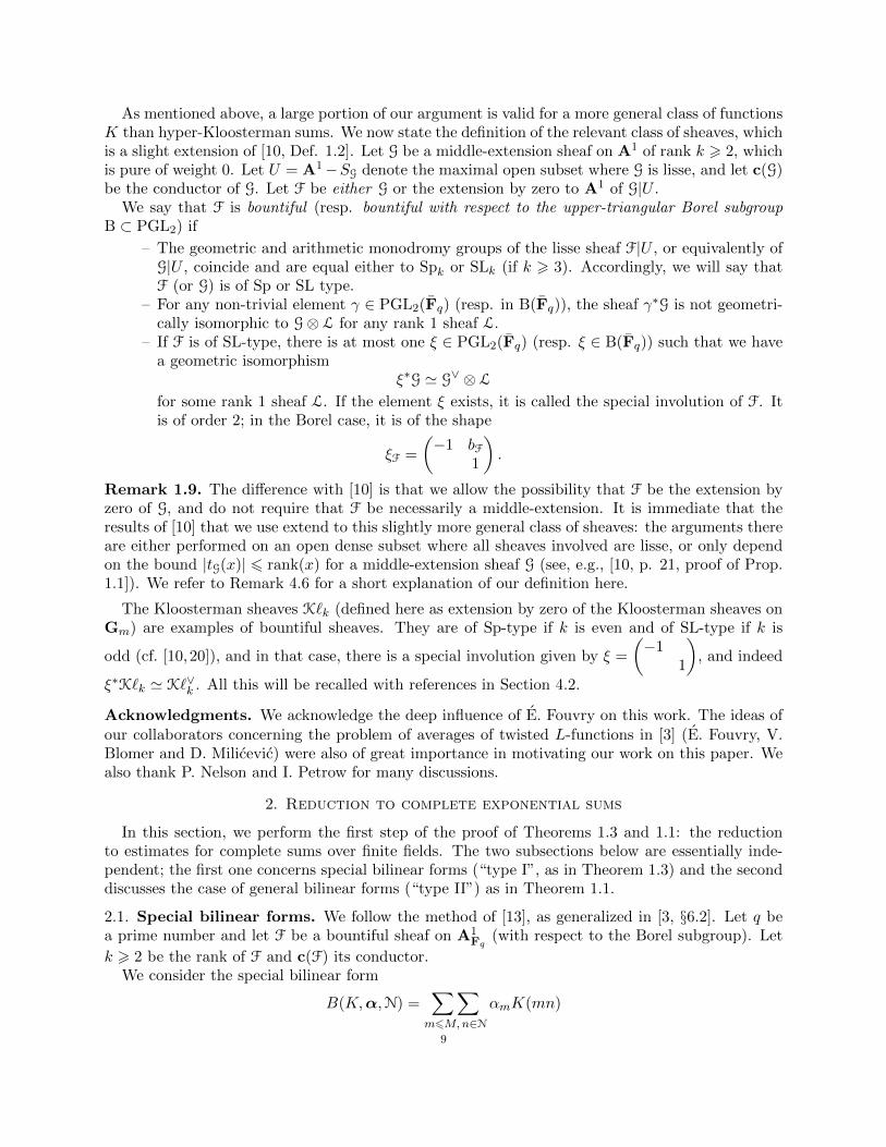
As mentioned above, a large portion of our argument is valid for a more general class of functionsK than hyper-Kloosterman sums. We now state the definition of the relevant class of sheaves, whichis a slight extension of [10, Def. 1.2]. Let G be a middle-extension sheaf on A1 of rank k > 2, whichis pure of weight 0. Let U = A1−SG denote the maximal open subset where G is lisse, and let c(G)be the conductor of G. Let F be either G or the extension by zero to A1 of G|U .

We say that F is bountiful (resp. bountiful with respect to the upper-triangular Borel subgroupB ⊂ PGL2) if

– The geometric and arithmetic monodromy groups of the lisse sheaf F|U , or equivalently ofG|U , coincide and are equal either to Spk or SLk (if k > 3). Accordingly, we will say thatF (or G) is of Sp or SL type.

– For any non-trivial element γ ∈ PGL2(Fq) (resp. in B(Fq)), the sheaf γ∗G is not geometri-cally isomorphic to G⊗ L for any rank 1 sheaf L.

– If F is of SL-type, there is at most one ξ ∈ PGL2(Fq) (resp. ξ ∈ B(Fq)) such that we havea geometric isomorphism

ξ∗G ' G∨ ⊗ L

for some rank 1 sheaf L. If the element ξ exists, it is called the special involution of F. Itis of order 2; in the Borel case, it is of the shape

ξF =

(−1 bF

1

).

Remark 1.9. The difference with [10] is that we allow the possibility that F be the extension byzero of G, and do not require that F be necessarily a middle-extension. It is immediate that theresults of [10] that we use extend to this slightly more general class of sheaves: the arguments thereare either performed on an open dense subset where all sheaves involved are lisse, or only dependon the bound |tG(x)| 6 rank(x) for a middle-extension sheaf G (see, e.g., [10, p. 21, proof of Prop.1.1]). We refer to Remark 4.6 for a short explanation of our definition here.

The Kloosterman sheaves K`k (defined here as extension by zero of the Kloosterman sheaves onGm) are examples of bountiful sheaves. They are of Sp-type if k is even and of SL-type if k is

odd (cf. [10,20]), and in that case, there is a special involution given by ξ =

(−1

1

), and indeed

ξ∗K`k ' K`∨k . All this will be recalled with references in Section 4.2.

Acknowledgments. We acknowledge the deep influence of E. Fouvry on this work. The ideas ofour collaborators concerning the problem of averages of twisted L-functions in [3] (E. Fouvry, V.Blomer and D. Milicevic) were also of great importance in motivating our work on this paper. Wealso thank P. Nelson and I. Petrow for many discussions.

2. Reduction to complete exponential sums

In this section, we perform the first step of the proof of Theorems 1.3 and 1.1: the reductionto estimates for complete sums over finite fields. The two subsections below are essentially inde-pendent; the first one concerns special bilinear forms (“type I”, as in Theorem 1.3) and the seconddiscusses the case of general bilinear forms (“type II”) as in Theorem 1.1.

2.1. Special bilinear forms. We follow the method of [13], as generalized in [3, §6.2]. Let q bea prime number and let F be a bountiful sheaf on A1

Fq(with respect to the Borel subgroup). Let

k > 2 be the rank of F and c(F) its conductor.We consider the special bilinear form

B(K,α,N) =∑∑m6M,n∈N

αmK(mn)

9

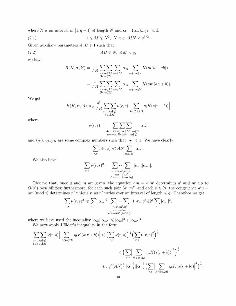
where N is an interval in [1, q − 1] of length N and α = (αm)m6M with

(2.1) 1 6M 6 N2, N < q, MN < q3/2.

Given auxiliary parameters A,B > 1 such that

(2.2) AB 6 N, AM < q,

we have

B(K,α,N) =1

AB

∑∑A<a62AB<b62B

∑m6M

αm∑

n+ab∈NK(m(n+ ab))

=1

AB

∑∑A<a62AB<b62B

∑m6M

αm∑

n+ab∈NK(am(an+ b)).

We get

B(K,α,N)�εqε

AB

∑∑r (mod q)s6AM

ν(r, s)∣∣∣ ∑B<b62B

ηbK(s(r + b))∣∣∣

where

ν(r, s) =∑∑∑

A<a62A, m6M, n∈Nam=s, an≡r (mod q)

|αm|

and (ηb)B<b62B are some complex numbers such that |ηb| 6 1. We have clearly∑r,s

ν(r, s)� AN∑m6M

|αm|.

We also have ∑r,s

ν(r, s)2 =∑· · ·∑

a,m,n,a′,m′,n′

am=a′m′a′n=an′ (mod q)

|αm||αm′ |.

Observe that, once a and m are given, the equation am = a′m′ determines a′ and m′ up toO(qε) possibilities; furthermore, for each such pair (a′,m′) and each n ∈ N, the congruence a′n =an′ (mod q) determines n′ uniquely, as n′ varies over an interval of length 6 q. Therefore we get∑

r,s

ν(r, s)2 �∑a,m

|αm|2∑· · ·∑

n,a′,m′,n′

am=a′m′a′n=an′ (mod q)

1�ε qεAN

∑m

|αm|2,

where we have used the inequality |αm||αm′ | 6 |αm|2 + |αm′ |2.We next apply Holder’s inequality in the form∑∑r (mod q)16s6AM

ν(r, s)∣∣∣ ∑B<b62B

ηbK(s(r + b))∣∣∣ 6 (∑

r,s

ν(r, s)) 1

2(∑r,s

ν(r, s)2) 1

4

×(∑r,s

∣∣∣ ∑B<b62B

ηbK(s(r + b))∣∣∣4) 1

4

�ε qε(AN)

34 ‖α‖

121 ‖α‖

122

(∑r,s

∣∣∣ ∑B<b62B

ηbK(s(r + b))∣∣∣4) 1

4.

10

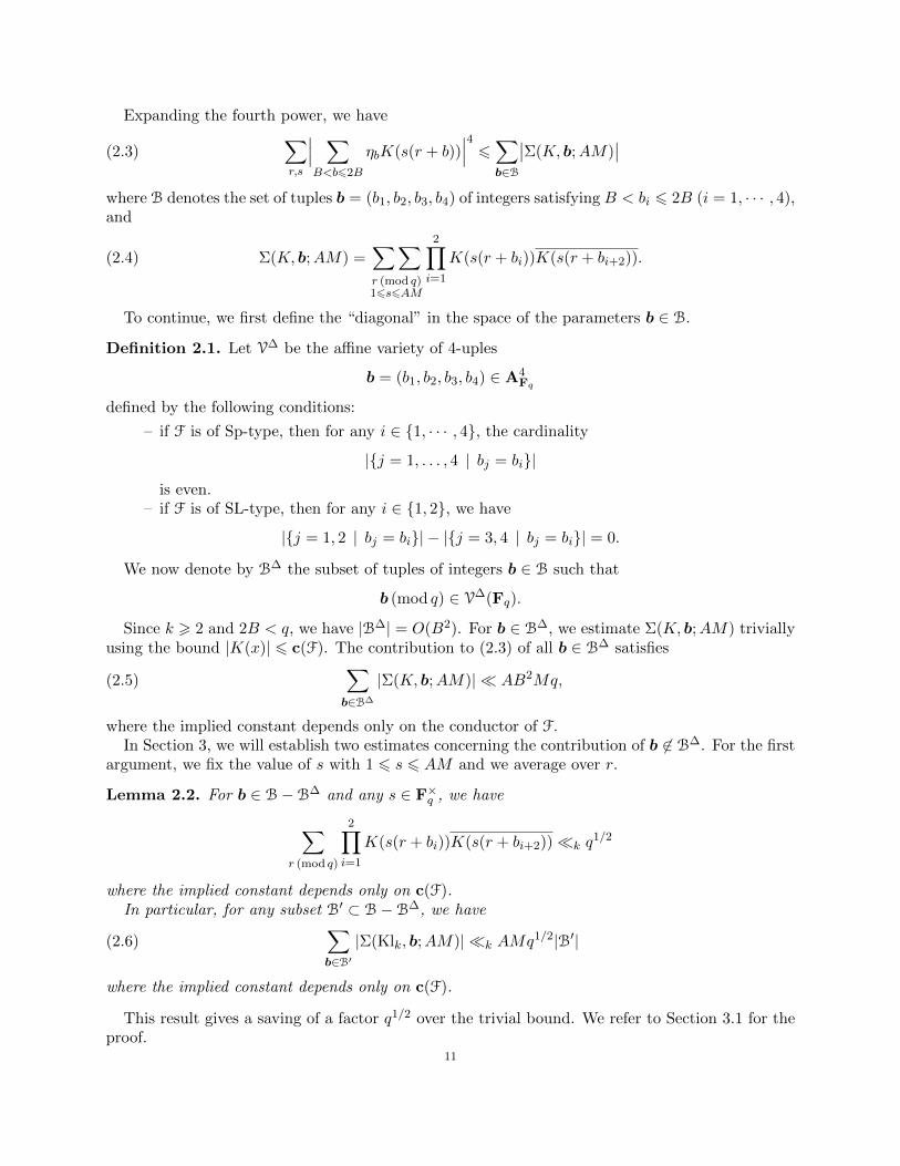
Expanding the fourth power, we have

(2.3)∑r,s

∣∣∣ ∑B<b62B

ηbK(s(r + b))∣∣∣4 6∑

b∈B

∣∣Σ(K, b;AM)∣∣

where B denotes the set of tuples b = (b1, b2, b3, b4) of integers satisfying B < bi 6 2B (i = 1, · · · , 4),and

(2.4) Σ(K, b;AM) =∑∑r (mod q)16s6AM

2∏i=1

K(s(r + bi))K(s(r + bi+2)).

To continue, we first define the “diagonal” in the space of the parameters b ∈ B.

Definition 2.1. Let V∆ be the affine variety of 4-uples

b = (b1, b2, b3, b4) ∈ A4Fq

defined by the following conditions:

– if F is of Sp-type, then for any i ∈ {1, · · · , 4}, the cardinality

|{j = 1, . . . , 4 | bj = bi}|

is even.– if F is of SL-type, then for any i ∈ {1, 2}, we have

|{j = 1, 2 | bj = bi}| − |{j = 3, 4 | bj = bi}| = 0.

We now denote by B∆ the subset of tuples of integers b ∈ B such that

b (mod q) ∈ V∆(Fq).

Since k > 2 and 2B < q, we have |B∆| = O(B2). For b ∈ B∆, we estimate Σ(K, b;AM) triviallyusing the bound |K(x)| 6 c(F). The contribution to (2.3) of all b ∈ B∆ satisfies

(2.5)∑b∈B∆

|Σ(K, b;AM)| � AB2Mq,

where the implied constant depends only on the conductor of F.In Section 3, we will establish two estimates concerning the contribution of b 6∈ B∆. For the first

argument, we fix the value of s with 1 6 s 6 AM and we average over r.

Lemma 2.2. For b ∈ B−B∆ and any s ∈ F×q , we have

∑r (mod q)

2∏i=1

K(s(r + bi))K(s(r + bi+2))�k q1/2

where the implied constant depends only on c(F).In particular, for any subset B′ ⊂ B−B∆, we have

(2.6)∑b∈B′|Σ(Klk, b;AM)| �k AMq1/2|B′|

where the implied constant depends only on c(F).

This result gives a saving of a factor q1/2 over the trivial bound. We refer to Section 3.1 for theproof.

11

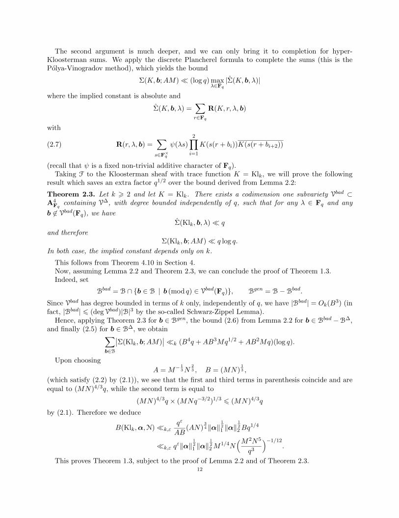
The second argument is much deeper, and we can only bring it to completion for hyper-Kloosterman sums. We apply the discrete Plancherel formula to complete the sums (this is thePolya-Vinogradov method), which yields the bound

Σ(K, b;AM)� (log q) maxλ∈Fq

|Σ(K, b, λ)|

where the implied constant is absolute and

Σ(K, b, λ) =∑r∈Fq

R(K, r, λ, b)

with

(2.7) R(r, λ, b) =∑s∈F×q

ψ(λs)

2∏i=1

K(s(r + bi))K(s(r + bi+2))

(recall that ψ is a fixed non-trivial additive character of Fq).Taking F to the Kloosterman sheaf with trace function K = Klk, we will prove the following

result which saves an extra factor q1/2 over the bound derived from Lemma 2.2:

Theorem 2.3. Let k > 2 and let K = Klk. There exists a codimension one subvariety Vbad ⊂A4

Fqcontaining V∆, with degree bounded independently of q, such that for any λ ∈ Fq and any

b 6∈ Vbad(Fq), we have

Σ(Klk, b, λ)� q

and thereforeΣ(Klk, b;AM)� q log q.

In both case, the implied constant depends only on k.

This follows from Theorem 4.10 in Section 4.Now, assuming Lemma 2.2 and Theorem 2.3, we can conclude the proof of Theorem 1.3.Indeed, set

Bbad = B ∩ {b ∈ B | b (mod q) ∈ Vbad(Fq)}, Bgen = B−Bbad.

Since Vbad has degree bounded in terms of k only, independently of q, we have |Bbad| = Ok(B3) (in

fact, |Bbad| 6 (degVbad)|B|3 by the so-called Schwarz-Zippel Lemma).Hence, applying Theorem 2.3 for b ∈ Bgen, the bound (2.6) from Lemma 2.2 for b ∈ Bbad −B∆,

and finally (2.5) for b ∈ B∆, we obtain∑b∈B

∣∣Σ(Klk, b;AM)∣∣�k (B4q +AB3Mq1/2 +AB2Mq)(log q).

Upon choosing

A = M−13N

23 , B = (MN)

13 ,

(which satisfy (2.2) by (2.1)), we see that the first and third terms in parenthesis coincide and are

equal to (MN)4/3q, while the second term is equal to

(MN)4/3q × (MNq−3/2)1/3 6 (MN)4/3q

by (2.1). Therefore we deduce

B(Klk,α,N)�k,εqε

AB(AN)

34 ‖α‖

121 ‖α‖

122Bq

1/4

�k,ε qε‖α‖

121 ‖α‖

122M

1/4N(M2N5

q3

)−1/12.

This proves Theorem 1.3, subject to the proof of Lemma 2.2 and of Theorem 2.3.12

2.2. General bilinear forms. We now consider the situation of Theorem 1.1. Again we beginwith a prime q and a bountiful sheaf F on A1

Fqwith respect to the Borel subgroup. Let k > 2 be

the rank of F and c(F) its conductor.Given M,N > 1 satisfying

(2.8) 1 6M 6 Nq1/4, q1/4 < MN < q5/4,

an interval N ⊂ [1, q − 1] of length N and sequences α = (αm)m6M and β = (βn)n∈N, we considerthe general bilinear form

B(K,α,β) =∑∑m6M,n∈N

αmβnK(mn).

We begin once more as in [3,13]. We choose auxiliary parameters A,B > 1 satisfying (2.2). Theargument of [3, §6.5] leads to the estimate

(2.9) |B(K,α,β)|2 � ‖α‖22‖β‖22(N +

qε

AB(AN)3/4M1/2

(∑b

|Σ 6=(K, b;AM)|)1/4)

for any ε > 0, where the implied constant depends only on c(F) and ε, and where

Σ 6=(K, b;AM) =∑

r (mod q)

∑∑16s1,s26AMs1 6≡s2 (mod q)

2∏i=1

K(s1(r + bi))K(s2(r + bi))K(s1(r + bi+2))K(s2(r + bi+2)

for b running over the set B of quadruples of integers (b1, b2, b3, b4) satisfying B < bi 6 2B.We will estimate the inner triple sum over r, s1, s2 in different ways depending on the value taken

by b.First, for b ∈ B∆ (as defined in Definition 2.1) we use a trivial bound and obtain

(2.10)∑b∈B∆

|Σ 6=(K, b;AM)| � qA2B2M2,

where the implied constant depends only on c(F).We next have an analogue of Lemma 2.2, where we sum over the variable r for fixed (s1, s2):

Lemma 2.4. For b ∈ B−B∆ and any s1, s2 ∈ F×q with s1 6= s2, we have

(2.11)∑

r (mod q)

2∏i=1

K(s1(r + bi))K(s2(r + bi))K(s1(r + bi+2))K(s2(r + bi+2)� q1/2,

where the implied constant depends only on c(F).In particular, for any subset B′ ⊂ B−B∆, we have∑

b∈B′|Σ 6=(K, b;AM)| � (AM)2|B′|q1/2,

where the implied constant depends only on c(F).

This is proved in Section 3.1.

Finally, we use discrete Fourier analysis. First, we detect the condition s1 6≡ s2 (mod q) usingadditive characters

1− 1

q

∑λ (mod q)

eq(λ(s1 − s2)) =

{1 if s1 6= s2 in Fq,

0 otherwise.

13

We further complete the sums over s1 and s2 using additive characters. This leads to the bound

Σ 6=(K, b;AM)� (log q)2 maxλ1,λ2∈Fq

|Σ(K, b, λ1, λ2)|

where

Σ(K,λ1, λ2, b) = C(λ1, λ2, b)−1

q

∑λ (mod q)

C(λ1 + λ, λ2 + λ, b),

in terms of the “correlation sums” given by

C(λ1, λ2, b) =∑

r (mod q)

R(r, λ1, b)R(r, λ2, b)

where R(r, λ, b) is the same sum already defined in (2.7).We must now assume as before that F = K`k is the Kloosterman sheaf of rank k with trace

function K = Klk. We will prove below our final bound:

Theorem 2.5. Let k > 2 and let K = Klk. There exists a codimension one subvariety Vbad ⊂ A4Fq

containing V∆, with degree bounded independently of q, such that for any b 6∈ Vbad(Fq) and everydistinct λ1, λ2 ∈ Fq, we have

(2.12) |Σ(Klk, λ1, λ2, b)| � q3/2

where the constant depends only on k.

This follows from Theorem 4.10 in Section 4. In fact, the subvariety Vbad is the same as inTheorem 2.3.

Assuming these results, we conclude the proof of Theorem 1.2 in the same manner as in theprevious section. For

Bbad = B ∩ {b ∈ B | b (mod q) ∈ Vbad(Fq)}, Bgen = B−Bbad,

we have the estimate |Bbad| = Ok(B3) since Vbad has degree bounded independently of q.

We apply Theorem 2.5 for b ∈ Bgen, the bound (2.11) of Lemma 2.4 for b ∈ Bbad − B∆ andfinally (2.10) for b ∈ B∆. This gives∑

b

|Σ 6=(Klk, b;AM)| � (log q)2(B4q3/2 +A2B3M2q1/2 +A2B2M2q),

where the implied constant depends only on k.We select

A = q18M−

12N

12 , B = q−

18M

12N

12 ,

which satisfy (2.2) by (2.8). Then AB = N and the first and third terms on the right-hand side

are equal to (MN)2q. The second term is (MN)52 q

38 6 (MN)2q by (2.8). Therefore we have∑

b

|Σ 6=(Klk, b;AM)| � (MN)2q(log q)2

and consequently we obtain from (2.9) the bound

|B(Klk,α,β)|2 � ‖α‖22‖β‖22(N +

qε

N(AN)3/4M1/2q1/4(MN)1/2

)� qε‖α‖22‖β‖22

(N + (MN)

58 q

1132

)� qε‖α‖22‖β‖22MN

(M−1 + (MN)−

38 q

1132

),

for any ε > 0, where the implied constant depends only on k and ε.This concludes the proof of Theorem 1.1 modulo the proof of Lemma 2.4 and of Theorem 2.5.

14

Remark 2.6. As in [13] it is possible to apply the Holder inequality that leads to (2.9) with higherexponent than 2l = 4. Doing this leads to sums involving products of the shape

(r, s1, s2) 7→l∏

i=1

K(s1(r + bi))K(s2(r + bi))K(s1(r + bi+l))K(s2(r + bi+l)

for

bl = (b1, · · · , bl, bl+1, · · · , b2l) ∈]B, 2B]2l.

Except for heavier notational complexity, some of the arguments of this section (and of the next)

do carry over and (assuming that (2.8) holds), one obtains for l > 3 and MN > q7/8 the bound

|B(Klk,α,β)|2 �ε,k qε‖α‖22‖β‖22MN

(M−1 + (ql+4(MN)−8)

14l(l+2)

).

This bound is only interesting when l = 3 and yields a non-trivial estimate in the range

MN > q78

+δ, δ > 0

compared with MN > q1112

+δ in Remark 1.2.In order for the Holder inequality with higher exponents to give better estimates, one needs

to improve the lower bound on the codimension of the variety Vbadl ⊂ A2lFq

in the corresponding

generalization of Theorem 2.5. At the moment, we only know that this codimension is at least1, but if one could prove that this variety has codimension 2, one could take l = 5 and obtain a

non-trivial bound in the range MN > q56

+δ.The best possible result which might be achieved using this method would be if Vbadl had codi-

mension l. This would lead to non-trivial bounds for

MN > q3l+5

4(l+1)+δ, δ > 0.

By taking l very large, we thus see that the limit of the method is the range MN > q34

+δ.Interestingly, this is the same range achieved in [11, Th. 1.6] for the case where α and β are bothsmooth.

3. Bounds for complete exponential sums

In this section we use methods from `-adic cohomology to prove Lemmas 2.2 and 2.4, and wemake the first steps towards Theorems 2.3 and 2.5. The proof of these last two theorems will befinished in Section 4.

All results in this section apply for bountiful sheaves (with respect to the Borel subgroup). Thuswe fix a prime q and such a sheaf F on A1

Fq. We denote by K the trace function of F, and by

SF ⊂ P1(Fq) the set of ramification points of F.For any finite extension Fqd/Fq, any b ∈ (Fqd)

4 and r ∈ Fqd , any (r, s) ∈ Fqd × Fqd , we denote

K(r, s, λ, b; Fqd) = ψFqd

(λs)

2∏i=1

K(s(r + bi); Fqd)K(s(r + bi+2); Fqd).

For d = 1, we write simply K(r, s, λ, b) = K(r, s, λ, b; Fq).15

3.1. One variable bounds. The next proposition is a restatement of Lemma 2.2 and 2.4.

Proposition 3.1. Assume q 6= 2. Let V∆ ⊂ A4Fq

be the affine variety given in Definition 2.1.

For all b = (b1, b2, b3, b4) ∈ Fq4 − V∆(Fq) and for all s, s1, s2 ∈ F×q , with s1 6= s2, we have∑

r∈Fq

K(r, s, 0, b)� q1/2,(3.1)

∑r∈Fq

K(r, s1, 0, b)K(r, s2, 0, b)� q1/2(3.2)

where the constant implied depend only on the conductor of F.

Proof. This follows from the techniques surveyed in [10]. Precisely, for fixed s ∈ F×q and b /∈ V∆(Fq),the sum in (3.1) is of the type discussed in [10, Cor. 1.6] with k = 4, h = 0, the 4-tuple

γ = (γs,1, · · · , γs,4) ∈ PGL2(Fq)4

such that

γs,i =

(s sbi

1

), i = 1, . . . , 4.

and (if F is of SL-type) the 4-tuple

σ = (σi)i=1,··· ,4 ∈ Aut(C/R)4

where

σ1 = σ2 = IdC, σ3 = σ4 = c, c = complex conjugation.

If F is of Sp type, the fact that b is not contained in V∆(Fq) implies that the tuple γ is normalin the sense of [10, Definition 1.3].

Similarly, if F is of SL-type with rank(F) = r > 3, and b 6∈ V∆(Fq), the pair of tuples (γ, σ)is r-normal, including with respect to the special involution ξF of F, if the latter exists. Indeed,because q 6= 2, γs,iγ

−1s,j is not an involution unless i = j, so can only be equal to ξF if i = j. This

means that conditions (2) and (3) of [10, Def. 1.3] are equivalent in our situation. Thus the bound(3.1) follows from [10, Cor. 1.6].

We now consider the bound (3.2). We are again in the situation of [10, Cor. 1.6] with h = 0,k = 8, the 8-tuple

γ = (γs1,1, . . . , γs1,4, γs2,1, . . . , γs2,4)

and (in the SL-type case) the 8-tuple

σ = (IdC, IdC, c, c, c, c, IdC, IdC).

For s1 6= s2 and b 6∈ V∆(Fq), the 8-tuple γ is normal for F of Spk-type while for F of SLr-type with r > 3, the tuples (γ,σ) are again r-normal (also possibly with respect to the specialinvolution ξF, it is exists). Indeed, the fact that s1 6= s2 implies that the multiplicities involvedin checking [10, Def. 1.3] are either multiplicities from the 4-tuple associated to s1, or from thatassociated to s2, and we are reduced to the situation in (3.1). Hence we obtain (3.2) by [10, Cor.1.6]. �

By definition, the bound (3.1) gives Lemma 2.2, and (3.2) gives Lemma 2.4.

Remark 3.2. In the case of hyper-Kloosterman sums (K = Klk), see also [10, Cor. 3.2, Cor. 3.3]for the statements we use concerning cancellation.

16

3.2. Second moment computations. We now consider second moment averages. These esti-mates will be used in the next section to prove irreducibility of various sheaves.

For any finite extension Fqd/Fq, any b ∈ (Fqd)4 and r ∈ Fqd , we define

(3.3) R(r, λ, b; Fqd) =∑s∈F

qd

K(r, s, λ, b; Fqd).

Note that, as a function of λ, this is the discrete Fourier transform of s 7→ K(r, s, 0, b; Fqd).

Lemma 3.3. Suppose that the bi, 1 6 i 6 4, are pairwise distinct in Fq. For any d > 1, we have

(3.4)1

(qd)2

∑∑r,λ∈F

qd

|R(r, λ, b; Fqd)|2 = qd +O(qd/2),

where the implied constant depends only on the conductor of F.

If F is of SL-type and admits the special involution ξ =

(−1 00 1

), then we have

(3.5)1

(qd)2

∑r,λ∈F

qd

R(r, λ, b; Fqd)R(r,−λ, b; Fqd) = O(qd/2),

where the implied constant depends only on the conductor of F.

Proof. We abbreviate simply ψ = ψFqd

and K(x) = K(x; Fqd) in the computations. Opening the

squares in the respective sums and averaging over λ, these sums are equal to

q−d∑

r,s∈Fqd

|K(r, s, 0, b; Fqd)|2 = q−d∑r∈F

qd

4∏i=1

|K(s(r + bi))|2

= q−d∑

r,s∈Fqd

r+bi 6=0, i=1,...,4

4∏i=1

|K(s(r + bi))|2 +O(1)

and

q−d∑

r,s∈Fqd

K(r, s, 0, b; Fqd)K(r,−s, 0, b; Fqd)

= q−d∑

r,s∈Fqd

2∏i=1

K(s(r + bi))K(s(r + bi+2))K(−s(r + bi))K(−s(r + bi+2))

= q−d∑

r,s∈Fqd

r+bi 6=0, i=1,...,4

2∏i=1

K(s(r + bi))K(s(r + bi+2))K(−s(r + bi))K(−s(r + bi+2)) +O(1)

respectively, where the implied constant depends only on the conductor of F.Since ξ∗F is geometrically isomorphic to the tensor product of the dual of F with a rank 1 sheaf

L, by assumption, it follows that K(−x) = χ(x)K(x) for some function χ with |χ(x)| = 1 for all xsuch that F is lisse at x. Hence the last sum is equal to

q−d∑

r,s∈Fqd

r+bi 6=0, i=1,...,4

L(x)4∏i=1

K(s(r + bi))2 +O(1).

17

where

L(x) =

2∏i=1

χ(s(r + bi))χ(s(r + bi+2)

is the trace function of a rank 1 sheaf. Using the relation ξ∗F ' F∨⊗L, we see that the conductorof L is bounded in terms of the conductor of F only.

We proceed to evaluate the sum over s using again [10] (more precisely, the final estimates followfrom the extension to all finite fields of these results, which is immediate).

For each i, let

γr+bi =

(r + bi 0

0 1

).

In the Sp-type case, since the r + bi are pairwise distinct for 1 6 i 6 4, the 8-tuple

γ = (γr+b1 , . . . , γr+b4 , γr+b1 , . . . , γr+b4)

consists of 4 pairs (γ, γ) elements; by [10, Cor. 1.7 (1)], it follows that for each r distinct from the−bi for 1 6 i 6 4, we have ∑

s∈Fqd

4∏i=1

|K((r + bi)s)|2 = qd +O(qd/2),

and summing over r gives (3.4).In the SL-type case with r = rank(F) > 3, the components of the pair of 8-tuples

γ = (γr+b1 , . . . , γr+b4 , γr+b1 , . . . , γr+b4)

σ = (IdC, IdC, IdC, IdC, c, c, c, c)

satisfy the final assumption of [10, Cor. 1.7 (2)], and hence∑s∈F

qd

4∏i=1

|K((r + bi)s)|2 = qd +O(qd/2).

also follows if r + bi is non-zero for each i. We therefore derive (3.4) again.Finally, in the SL-type with the special involution ξ as above, the pair of 8-tuples

γ = (γr+b1 , . . . , γr+b4 , γr+b1 , . . . , γr+b4)

σ = (IdC, . . . , IdC)

is r-normal with respect to ξ (because the multiplicity of any element in the tuple is either 0 or 2).Arguing as in the proof of [10, Th. 1.5] (p. 20–21, loc. cit.), we deduce that for each r distinctfrom the −bi for 1 6 i 6 4, we have∑

s∈Fqd

L(x)4∏i=1

K(s(r + bi))2 � qd/2,

where the implied constant depends only on the conductor of F. �

Finally, we consider one more averaging over the r and b variables in the case when λ = 0.

Lemma 3.4. For any d > 1, we have

1

(qd)5

∑∑(r,b)∈F5

qd

|R(r, 0, b; Fqd)|2 = qd +O(qd/2)

where the implied constant depends only on the conductor of F.

18

Proof. By a change of variables, we see that the sum is given by

q−4d∑∑b1,b2,b3,b4

∣∣∣ ∑s∈F×

qd

2∏i=1

K(sbi; Fqd)K(sbi+2; Fqd)∣∣∣2 =

∑s,s′∈F×

qd

|C(K, s, s′; Fqd)|2|C(K, s′, s; Fqd)|2

where

C(K, s, s′; Fqd) = q−d∑b∈F

qd

K(sb; Fqd)K(s′b; Fqd) = q−d∑b∈F

qd

K((s/s′)b; Fqd)K(b; Fqd).

By assumption, the sheaf F is geometrically irreducible and is such that [×s/s′]∗F is geometricallyisomorphic to F if and only if s = s′. Therefore by the usual application of the Riemann Hypothesis(see Proposition 1.8), we have

C(L, s, s′; Fqd) = δ(s, s′) +O(q−d/2),

where the implied constant depends only on the conductor of F. It follows that∑s,s′∈F×

qd

|C(K, s, s′; Fqd)|2|C(K, s′, s; Fqd)|2 = qd +O(qd−d/2) +O(q2d−4d/2) = qd +O(qd/2),

were the implied constant depends only on the conductor of F. �

4. Irreducibility of Vinogradov-Kloosterman sheaves

The goal of this long section, which is the most difficult of the paper, is to prove Theorems 2.3and 2.5. For the whole, we fix a prime q and a non-trivial additive character ψ of Fq.

We first begin by outlining the argument. The 7-variable function K and its sum R associatedto the trace function of a sheaf F are first interpreted as trace functions of suitables sheaves inSection 4.1. The goal is then to prove that various specializations of these sheaves, which we callVinogradov sheaves, are geometrically irreducible. This we can do when F is a Kloosterman sheaf.To do so requires quite delicate properties of these sheaves, which are recalled in Section 4.2. Italso requires some relatively general tools which are stated for convenience in Section 4.3. Theargument splits in two parts, depending on whether we specialize with λ = 0 or with λ 6= 0, andthese are handled separately in Sections 4.4 and 4.5.

4.1. Vinogradov sheaves. Let F be an Q`-sheaf on A1Fq

, lisse of rank k and pure of weight 0 on

a nonempty open subset, and mixed of weight 6 0 on A1. (Examples of this include the extensionby zero of a lisse and pure sheaf from an open subset or the middle extension of a lisse and puresheaf [6, Corollary 1.8.9].)

On the affine space A7 = A2 × A × A4, with coordinates denoted (r, s, λ, b), we define theprojection p2,3 : A7 −→ A1 by

p2,3(r, s, λ, b1, . . . , b4) = λs

and morphisms fi : A7 −→ A1 for 1 6 i 6 4 by

(4.1) fi(r, s, λ, b1, . . . , b4) = s(r + bi).

Let K be the Q`-sheaf on A7 defined by

(4.2) K = p∗2,3Lψ ⊗2⊗i=1

(f∗i F ⊗ f∗i+2F∨).

19

The sheaf K is a constructible Q`-sheaf of rank k4 on A7, pointwise mixed of weights 6 0. Itis lisse and pointwise pure of weight 0 on the dense open set UK which is the complement of theunion of the divisors given by the equations

{s = 0} and {s(r + bi) = µ}, for µ ∈ SF and i = 1, . . . , 4,

where SF is the set of ramification points of F in A1. The trace function of K is

tK(r, s, λ, b) = K(r, s, λ, b)

for (r, s, λ, b) ∈ UK(Fq).

Now we consider the projection π(2) : A7 −→ A6 given by

π(2)(r, s, λ, b) = (r, λ, b),

and the compactly-supported higher-direct image sheaves Riπ(2)! K. Since the fibers of π(2) are

curves, these sheaves are zero unless 0 6 i 6 2.

Lemma 4.1. Assume that the sheaf F is bountiful with respect to the Borel subgroup.

(1) For 0 6 i 6 2, the sheaf Riπ(2)! K on A6

Fqis mixed of weights 6 i.

(2) Let V= be the subvariety of A4 given in Definition 2.1. The sheaves R0π(2)! K and R2π

(2)! K

are supported on A1 ×A1 × V=.

Proof. The first part is an application of Deligne’s main theorem [6, Theorem 1]. For the second

part, by the proper base change theorem, the stalk of R0π(2)! K at x = (r, λ, b) ∈ A7 is

H ic(A

1/Fq,Lψ(sλ) ⊗2⊗i=1

[×(r + bi)]∗K⊗ [×(r + bi+2]∗K∨)

where s is the coordinate on A1.This cohomology group vanishes for i = 0 and any x. For i = 2 and x /∈ V=, its vanishing is

given by [10, Theorem 1.5] using (only) the assumption that F is bountiful in these sense of ourdefinition. �

The sheaf R1π(2)! K, which is mixed of weights at most 1, is almost the sheaf we want to under-

stand. However, some cleaning-up is required to facilitate the later arguments. Precisely, recall(see [6, Th. 3.4.1 (ii)]) that a lisse sheaf which is mixed of weight 6 w is an extension of a lissesheaf which is pure of weight w by a mixed sheaf of weight 6 w − 1. Thus the following definitionmakes sense:

Definition 4.2 (Vinogradov sheaf). Let F be a bountiful sheaf on A1Fq

, and let K be the sheaf (4.2)

and R = R1π(2)! K. Let (Xi) be a stratification of A6

Fqby locally closed subsets such that R is lisse

on each strat. We define the Vinogradov sheaf R∗ associated to F as the constructible sheaf givenas the sum over Xi of the maximal quotient of R|Xi which is pure of weight 1 extended by zero toall of A6

Fq, so that R∗|Xi is the maximal pure of weight 1 quotient of R|Xi. (Any sheaf satisfying

that condition would work for our arguments.)For any (λ, b) ∈ A5, we denote by R∗λ,b the pullback of R∗ to the affine line given by the morphism

r 7→ (r, λ, b), and we call R∗λ,b a specialized Vinogradov sheaf.

By construction, the Vinogradov sheaf is punctually pure of weight 1. A first property of thissheaf is as follows:

20

Proposition 4.3. For any d > 1, we have

1

(qd)5

∑∑(r,b)∈F5

qd

|tR∗(r, 0, b; Fqd)|2 = qd +O(qd/2).

Proof. SincetR∗(r, 0, b; Fqd) = tR(r, 0, b; Fqd) +O(1),

by construction, it is enough to prove that

1

(qd)5

∑∑(r,b)∈F5

qd

|tR(r, 0, b; Fqd)|2 = qd +O(qd/2).

Let V∆ be the subvariety of A4 defined in Definition 2.1. We have∑∑(r,b)∈F5

qd

|R(r, 0, b; Fqd)|2 =∑∑(r,b)∈F5

qd

b6∈V∆(Fqd

)

|R(r, 0, b; Fqd)|2 +∑∑(r,b)∈F5

qd

b∈V∆(Fqd

)

|R(r, 0, b; Fqd)|2.

Since V∆ has codimension 2 and R(r, 0, b; Fqd)�k qd, the second sum is bounded by �k q

4d. Onthe other hand, the first sum equals ∑∑

(r,b)∈F5qd

b6∈V∆(Fqd

)

|tR(r, 0, b; Fqd)|2.

By the same argument we get∑∑(r,b)∈F5

qd

b6∈V∆(Fqd

)

|tR(r, 0, b; Fqd)|2 =∑∑(r,b)∈F5

qd

|tR(r, 0, b; Fqd)|2 +O(q4d),

and the result then follows from Lemma 3.4. �

We also have the following general duality property that will be convenient later on.

Lemma 4.4. For b = (b1, b2, b3, b4) ∈ A4, let b = (b3, b4, b1, b2). For any λ and b /∈ V=, thereexists an isomorphism

R∗∨λ,b ' R∗−λ,b(1)

on any dense open subset where R∗λ,b is lisse.

Proof. Let U be a dense open subset where R∗λ,b is lisse. Let d > 1 and x ∈ U(Fqd) be given. Wefirst observe that

tR∗−λ,b

(x; Fqd) = tR−λ,b(x; Fqd) +O(1) = R(x,−λ, b) +O(1)

= R(x, λ, b) +O(1) = tRλ,b(x; Fqd) +O(1) = tR∗λ,b(x; Fqd) +O(1).

Since R∗λ,b is pure of weight 1 on U , we have further

tR∗∨λ,b(x; Fqd) =1

qdtR∗λ,b(x; Fqd) =

1

qdtR∗−λ,b

(x; Fqd) +O(q−d).

Since the sheaves involved are pointwise pure, and geometrically semisimple (by a result ofDeligne [6, Th. 3.4.1 (iii)]), Deligne’s equidistribution theorem implies that there is an isomorphism

R∗∨λ,b ' R∗−λ,b(1).

21

�

4.2. Properties of Kloosterman sheaves. We will study the Vinogradov sheaves associated toKloosterman sheaves. We summarize the basic properties of these sheaves, which were originallydefined by Deligne.

Proposition 4.5 (Kloosterman sheaves). Let q be a prime number, ` 6= q an auxiliary primenumber and ψ a non-trivial `-adic additive character of Fq. Let k > 1 be an integer.

There exists a constructible Q`-sheaf K` = K`ψ,k on P1Fq

, with the following properties:

(1) For any d > 1 and any x ∈ Gm(Fqd), we have

tK`(x; Fqd) = Klk(x; Fqd) =(−1)k

qd(k−1)/2

∑x1···xk=x

ψFqd

(x1 + · · ·+ xk);

(2) It is lisse of rank k on Gm;(3) On Gm it is geometrically irreducible and pure of weight 0.(4) It is tamely ramified at 0 with unipotent local monodromy with a single Jordan block;(5) It is wildly ramified at ∞, with a single break equal to 1/k, and Swan conductor 1;(6) The dual sheaf K`∨ψ,k is given by

K`∨ψ,k ' [x 7→ (−1)kx]∗K`ψ,k

where the isomorphism is arithmetic; in particular, K`ψ,k is arithmetically self-dual if k iseven;

(7) If k > 2, then the arithmetic and geometric monodromy groups of K`ψ,k are equal; if k iseven, they are equal to Spk and if k is odd, then they are equal to SLk;

(8) Its stalks at 0 and ∞ both vanish.(9) If γ ∈ PGL2(Fq) is non-trivial, there does not exist a rank 1 sheaf L such that we have a

geometric isomorphism over a Zariski open set

γ∗K`ψ,k ' K`ψ,k ⊗ L.

Proof. All this is essentially mise pour memoire from [20], where our sheaf is denoted Kln(ψ)((k−1)/2) in [20, 11.0.2]; precisely, properties (1) to (5) are stated with references in [20, 11.0.2], property(6) is found in [20, Cor. 4.1.3, Cor. 4.1.4], and the crucial property (7) is [20, Th. 11.1, Cor. 11.3].The sheaf constructed in [20] is on Gm, and we extend by zero from Gm to P1, making property(8) true by definition. The last property is explained, e.g., in [10, §3, (b), (c)]. �

Remark 4.6. (1) As a matter of definition, one possibility is to define K`ψ,k as k-fold (Tate-twisted)multiplicative convolution of the basic Artin-Schreier sheaf Lψ, namely

K`k = (Lψ ? · · · ? Lψ)((k − 1)/2),

see [20, 5.5].(2) Katz has also shown (see [20, Cor. 4.1.2]) that the property (1) characterizes K`ψ,k as a lisse

sheaf on Gm, up to arithmetic isomorphism.(3) It might seem more natural to define K`ψ,k as the middle extension from Gm to P1 of the

sheaf constructed by Katz. However, the property of being a middle extension is not preserved bytensor product, so we would not be able to use directly any of the properties of middle extensionsheaves when studying K. On the other hand, having stalk zero is preserved by tensor product, itwill turn out that this property simplifies certain technical arguments.

22

Corollary 4.7. For k > 2, the sheaf K`ψ,k is bountiful in the strong sense; it is of Sp-type if k

is even, and of SL-type if k is odd. In the second case, K`ψ,k has the special involution

(−1 00 1

).

Moreover, the conductor of K`ψ,k is bounded in terms of k only.

Proof. This is clear from Proposition 4.5 using the definition of bountiful sheaves and of the con-ductor of a sheaf. �

For convenience, we will most often simply denote K` = K`ψ,k since we assume that k and ψare fixed. We also sometimes write F = K`, when stating properties of a “generic” nature that weexpect to hold for much more general classes of sheaves.

The following lemma gives a more precise description of the local monodromy of K`k at ∞.

Lemma 4.8. Assume q > k > 1. Denote by ψ the additive character x 7→ ψ(x/k) of Fq. Then, asrepresentations of the inertia group I(∞) at ∞, there exists an isomorphism

K`k ' [x 7→ xk]∗(Lχk+12⊗ Lψ),

where we recall that χ2 is the unique non-trivial character of order 2 of F×q .

Proof. According to the remark in [20, 10.4.5], we have an isomorphism

K`k ' [x 7→ xk]∗(Lψ),

as a representation of the wild inertia subgroup P (∞) ⊂ I(∞). On the other hand, by [21, Theorem8.6.3], an I(∞)-representation which is totally wild with Swan conductor 1 is determined, up toscaling, by its rank and its determinant (i.e., if two such representations π1 and π2 have same rankand determinant, then there exists a non-zero c such that π2 ' [×c]∗π1).

Since detK` is trivial (see Proposition 4.5 (7)), it is therefore sufficient to check that the deter-minant of the I(∞)-representation [x 7→ xk]∗(Lχk+1

2⊗ Lψ) is trivial.

But for any multiplicative character χ, we have a geometric isomorphism

det([x 7→ xk]∗(Lχ ⊗ Lψ)) ' χχk+12

and this is geometrically trivial if χ = χk+12 (this follows, e.g., from the Hasse-Davenport relations

as in [20, Proposition 5.6.2], or from the block-permutation matrix representation of an inducedrepresentation, similarly to the argument that appears later in Lemma 4.14). �

Finally, we can state our main theorem concerning the Vinogradov sheaves associated to Kloost-erman sheaves.

Theorem 4.9 (Irreducibility of Vinogradov-Kloosterman sheaves). Let k > 2 be an integer. Let qbe a prime, ` 6= q a prime and let R∗ be the `-adic Vinogradov sheaf associated to K`k over Fq.

If q is sufficiently large with respect to k, there exists a closed subset Vbad ⊂ A4Fq

of codimen-

sion 1 and of degree bounded independently of q, stable under the automorphism (b1, b2, b3, b4) 7→(b3, b4, b1, b2), such that for all b = (b1, b2, b3, b4) not in Vbad, the following properties hold:

(1) For all λ, the specialized Vinogradov sheaf R∗λ,b is lisse and geometrically irreducible on a

dense open subset of A1;(2) For all λ, there does not exist a dense open subset U of A1 such that R∗λ,b|U is geometrically

trivial;(3) If λ 6= λ′, then there does not exist a dense open subset U of A1 such that R∗λ,b|U is

geometrically isomorphic to R∗λ′,b|U .23

(4) For all λ1, λ2, b1, b2, the dimensions of the stalks of the sheaf Rλi,bi, and the dimensionsof the cohomology groups H i

c(A1/Fq,Rλ1,b1) and H i

c(A1/Fq,Rλ1,b1⊗Rλ2,b2) are bounded in

terms of k only, in particular independently of q for k fixed.

The proof will occupy most of the remainder of this section. We first recall how this theoremimplies our desired Theorems 2.3 and 2.5.

Theorem 4.10. Let R(r, λ, b) be the function on A6(Fq) defined in (3.3). For any b ∈ F4q −

Vbad(Fq) and any λ, λ′ ∈ Fq, we have∑r∈Fq

R(r, λ, b)� q,

∑r∈Fq

R(r, λ, b)R(r, λ′, b) = δ(λ, λ′)q2 +O(q3/2),

where the implied constant depends only on k.

Proof. First of all, note that by the proper base change theorem and the Grothendieck-Lefschetztrace formula, we have

(4.3) tR(r, λ, b) = −∑s∈Fq

tK(r, s, λ, b) = −R(r, λ, b) +O(1)

for b /∈ V=, where the implied constant depends only on k. Since R is mixed of weights 6 1 and ofrank bounded in terms of k only, we have

tR(r, λ, b)� q1/2

for b /∈ V=.We begin the proof of the second bound. Thus let b ∈ F4

q − Vbad(Fq) and λ, λ′ ∈ Fq be

given. First, we have R(r, λ, b) = R(r,−λ, b), where b = (b3, b4, b1, b2) ∈ F4q − Vbad(Fq). Thus the

relation (4.3) and the Grothendieck-Lefschetz trace formula imply that∑r∈Fq

R(r, λ, b)R(r, λ′, b) =

2∑i=0

(−1)i Tr(

Frq | H ic(A

1/Fq,Rλ,b ⊗ R−λ′,b))

+O(q3/2)

where the implied constant depends only on k.Let F = Rλ,b⊗R−λ′,b and F∗ = R∗λ,b⊗R∗−λ′,b. Since R is mixed of weight 6 1, the tensor product

sheaf F is mixed of weight 6 2, so the i-th compactly supported cohomology group with coefficientin F is mixed of weight 6 i+ 2 by Deligne’s Theorem [6].

The dimension of these cohomology groups are bounded in terms of k only by Theorem 4.9 (4).Thus we have ∑

r∈Fq

R(r, λ, b)R(r, λ′, b) = Tr(Frq | Wλ,λ′) +O(q3/2)

where Wλ,λ′ is the subspace of weight 4 in H2c (A1/Fq,F) = H2

c (U/Fq,F), and the implied constantdepends only on k.

Let U be a dense open set where F is lisse. We have by definition a short exact sequence

0 −→ G −→ F −→ F∗ −→ 0

of lisse sheaves on U where G is mixed of weights < 2. Taking the long coholomogy exact sequenceand applying again Deligne’s Theorem, we see that Wλ,λ′ ' W ∗λ,λ′ , where W ∗λ,λ′ is the subspace of

weight 4 in H2c (U/Fq,F

∗).24

By the coinvariant formula, we have

H2c (U/Fq,F

∗) = (F∗η)π1(U)(−2),

so it is sufficient to prove that the weight 2 part of the π1(U)-coinvariants of F∗ has dimensionδ(λ, λ′), and that the action of Frq is multiplication by q when λ = λ′.

By Lemma 4.4, we have an isomorphism

R∗∨λ′,b ' R∗−λ′,b(1)

on U . This shows that it is sufficient to prove that the π1(U)-coinvariants of the sheaf R∗λ,b ⊗R∗∨λ′,b

have dimension δ(λ, λ′) and that Frq is the identity on this space when λ = λ′.But Rλ,b and Rλ′,b are geometrically irreducible by Theorem 4.9 (1), so the monodromy coinvari-

ants of that tensor product is one-dimensional if R∗λ,b and R∗λ′,b are geometrically isomorphic and is

zero otherwise. By Theorem 4.9 (3), the sheaves are geometrically isomorphic if and only if λ = λ′,and we get the dimension δ(λ, λ′). Finally, if λ = λ′, the space of coinvariants is one-dimensional,generated by the trace, on which Frq acts trivially.

The argument for the first bound is similar but simpler. We work with the cohomology groupsH ic(A

1/Fq,Rλ,b), which are mixed of weights 6 i+ 1. It is sufficient to show that the weight 3 partof H2

c (A1/Fq,Rλ,b) vanishes, and thus sufficient to show that the weight 1 part of the monodromycoinvariants of Rλ,b vanishes. Because R∗ is the weight 1 part of R, this is the same as showingthat the monodromy coinvariants of R∗λ,b vanishes. But R∗λ,b is irreducible and nontrivial as a

monodromy representation, by Theorem 4.9 (2) (3), so it has no coinvariants. �

4.3. Preliminaries. We collect in this section a number of results and definitions that we will usein the proof of our results. In a first reading, it might be easier to only survey the statements beforegoing to the next section.

We will ultimately derive the irreducibility statements of Theorem 4.9 from the following criteria.

Lemma 4.11. Let X,Y be normal varieties over a finite field Fq. Let f : Y −→ X be a smoothproper morphism whose fibers are curves. Let D ⊂ Y be a divisor.

For a lisse Q`-sheaf F on Y −D, consider the three following conditions:

(1) The sheaf F is geometrically irreducible and pure of some weight.(2) For the generic point η of X, the greatest common divisor of the multiplicities of the different

indecomposable subrepresentations of the different local monodromy representations at pointsof Dη of the restriction F|(Yη−Dη), counting Galois-conjugate representations as the same,is 1; for instance, one of the local monodromy representations of F|(Yη −Dη) at a point ofDη has an indecomposable component, defined over the base field, of multiplicity 1;

(3) The divisor D is smooth over X, and on each irreducible component of D, the Swan con-ductor function

x 7→ Swanx((F ⊗ F∨)|(Yf(x) −Df(x)))

is a constant function of x ∈ D.

Then the following statements are true:(a) If (1) and (2) hold, then for all x in a dense open subset of X, the restriction Fx = F|(Yx−Dx)

to a fiber Yx −Dx is geometrically irreducible.(b) If (1), (2) and (3) hold, then for all x in X, the restriction F|(Yx −Dx) to a fiber Yx −Dx

is geometrically irreducible.

The proof will clarify precisely the meaning of the second condition.

Proof. We assume that conditions (1) and (2) hold.25

Let η′ be the generic point of Y . By [33, V, Proposition 8.2], the natural homomorphismπ1(η′) −→ π1(Y ) is surjective. Since it factors through the natural homomorphism π1(Yη)→ π1(Y ),it follows that the latter is also surjective. In particular, condition (1) shows that the restriction ofF to Yη −Dη corresponds to an irreducible representation of π1(Yη). Thus Fη = F|(Yη −Dη) is anirreducible lisse sheaf on Yη −Dη.

Consider now a geometric point η over η, the geometric fibers Yη and Dη and the pullback Fη ofFη to (Y −D)η. We will show that condition (2) implies that Fη is irreducible.

Indeed, the representation of π1(Yη) corresponding to Fη is semisimple, as the restriction to anormal subgroup of an irreducible, hence semisimple, representation. Let

Fη =⊕i∈I

niVi

be a decomposition of this representation of π1(Yη) into irreducible subrepresentations, where ni > 1and the Vi are pairwise non-isomorphic. The quotient

G = π1(Yη)/π1(Yη),

which is isomorphic to the Galois group of the function field of the curve Yη, acts on the set {Vi}of irreducible subrepresentations. Since Fη is an irreducible representation of π1(Yη), this action istransitive. Hence, for any point y of Dη, the restriction of Fη to the decomposition group at y hasthe property that it is a direct sum of n =

∑ni subrepresentations which are G-conjugates (but

not necessarily irreducible or even indecomposable). In particular, any indecomposable subrepre-sentation of the decomposition group appears with multiplicity divisible by n.

But the meaning of condition (2) is that the greatest common divisor of the multiplicities ofany indecomposable subrepresentation of some local monodromy representation of Fη is 1. Thistherefore implies that n = 1, so that Fη is irreducible.

For a point x ∈ X, the fiber Fx is geometrically irreducible if and only if the cohomologygroup H2

c ((Y − D)x/Fq,Fx ⊗ F∨x ) is one-dimensional, by the coinvariant formula for the secondcohomology group on a curve (see, e.g., [20, 2.0.4]) and the fact that Fx ⊗ F∨x , being pure, isgeometrically semisimple (see [6, Th. 3.4.1 (iii)]). Equivalently, by the proper base change theorem,the specialized sheaf Fx is geometrically irreducible if and only if the stalk of R2f!(F ⊗ F∨) at xis one-dimensional. We have seen that the stalk is one-dimensional for x = η; since the sheafR2f!(F ⊗ F∨) is constructible, it is lisse on a dense open subset, and therefore the stalks are one-dimensional for all x in a dense open subset, which gives (a).

Now assume further that condition (3) holds. Then Deligne’s semicontinuity theorem [26, Corol-lary 2.1.2] implies that the sheaf R2f!(F ⊗ F∨) is lisse on X. Since it has rank 1 at the genericpoint, it has rank 1 on all of X, which means that Fx is geometrically irreducible for all x in X. �

Remark 4.12. Our proofs of condition (1) generalizes to quite general (bountiful) sheaves, butthe proofs of conditions (2) and (3) involve careful calculations that depend on specific propertiesof the Kloosterman sheaves. This means that our results do not easily generalize to other sheaves.

However, condition (2) is a “generic” condition that should hold for a “random” sheaf. Thus itshould be possible to prove it in a number of different concrete cases. The last condition (3) is moresubtle; although is always true on a dense open subset (hence is generic in that sense), the closedcomplement where it fails will usually have codimension 1. However, it should often be possible tocompute explicitly that subset, and to use this information for further study (cf. Remark 2.6 forinstance).

We will use the criteria of Lemma 4.11 for the proof of Theorem 4.9 in two different situations:(1) we will use (a) for specialized Vinogradov sheaves R∗0,b to show that, for all b = (b1, b2, b3, b4)

outside of a proper subvariety, these sheaves are geometrically irreducible; (2) we will use (b) to26

prove that for all b outside of a proper subvariety, the specialized sheaves R∗λ,b are geometricallyirreducible for every non-zero λ.

To verify the first condition of the lemma, we will use Katz’s diophantine criterion for geometricirreduciblity (compare [22, Lemma 7.0.3]).

Lemma 4.13 (Diophantine criterion for irreducibility). Let YFq be a normal variety, U ⊂ Y adense open subset and F a sheaf on Y that is lisse on U . Assume moreover that F|U is pure ofsome weight w > 0, and that F is mixed of weights 6 w on Y . Then F|U is geometrically irreducibleif

1

qd dimY

∑y∈Y (F

qd)

|tF(y)|2 = qdw(1 + o(1))

as d tends to infinity.

Proof. By twisting, we may assume that w = 0. Let n be the dimension of Y and D = Y −U . Wehave

1

qnd

∑y∈Y (F

qd)

|tF(y)|2 =1

qnd

∑y∈U(F

qd)

|tF(y)|2 +1

qnd

∑y∈D(F

qd)

|tF(y)|2.

The second sum is bounded by O(q−d) = o(1) using our assumption on the weights of F on Y (andthe reduction to w = 0), and hence the assumption implies that

1

qnd

∑y∈U(F

qd)

|tF(y)|2 → 1

as d → +∞. On the other hand, the Grothendieck–Lefschetz Trace Formula and the RiemannHypothesis imply that∑

y∈U(Fqd

)

|tF(y)|2 = Tr(FrFqd| H2n

c (Y/Fq,F ⊗ F∨)) +O(qd(n−1/2)),

and therefore1

qnd

∑y∈U(F

qd)

|tF(y)|2 = Tr(FrFqd| H2n

c (Y/Fq,F ⊗ F∨)(n)) + o(1)

By the coinvariant formula

H2nc (Y/Fq,F ⊗ F∨) ' (F ⊗ F∨)π(U/Fq)(−n),

and the semisimplicity of F (see [6, Th. 3.4.1 (iii)]), we deduce by combining these that thegeometric invariant subspace of F⊗F∨ is one-dimensional, which by Schur’s Lemma means that F

is geometrically irreducible. �

We will use the following lemma from elementary representation theory to describe the localmonodromy of tensor products of Kloosterman sheaves.

Lemma 4.14. Let G be a group and E an arbitrary field. Let H be a normal subgroup of G.Consider the usual action

V 7→ σ(V )

of G/H on E-representations of H, where x ∈ H acts on σ(V ) by the action of σ−1xσ on V .For any finite-dimensional E-representations V1, . . . , Vn of H, we have a canonical isomorphism

n⊗i=1

IndGH Vi '⊕

(σ2,...,σn)∈(G/H)n−1

IndGH

(V1 ⊗

n⊗i=2

σi(Vi)

).

27

Proof. We proceed by induction on n. The case n = 1 is a tautology. For n = 2, we need to provethat

IndGH V1 ⊗ IndGH V2 '⊕

σ∈G/H

IndGH (V1 ⊗ σ(V2))

To see this, first apply the projection formula

IndGH(V1 ⊗ ResHG IndGH V2) = IndGH V1 ⊗ IndGH V2

and then the fact thatResHG IndGH V2 =

⊕σ∈G/H

σ(V2),

which follows from the definition of induction (see, e.g., [25, Prop. 2.3.15, Prop. 2.3.18] for thesestandard facts).

We easily complete the proof for n > 3 by induction using the case n = 2. �

As a corollary, we now obtain the local monodromy at infinity for the sheaves Kr,λ,b. To state

the result, we recall from the introduction the notation Lψ(cs1/k), for a variety X/Fq, an integerk > 1 and a function c on X: this is the sheaf on X ×A1 (with coordinates (x, s)) given by

Lψ(cs1/k) = α∗Lψ(c(x)t)

where α is the covering map (x, s, t) 7→ (x, s) on the k-fold cover {(x, s, t) ∈ X×A1×A1 | tk = s}.

Lemma 4.15. Assume q > k and denote by ψ the character x 7→ ψ(x/k). Fix r, b, λ such that

r + bi 6= 0 for all i. Let (r + bi)1/k be a fixed k-th root of r + bi in Fq.

Then the local monodromy at s =∞ of Kr,λ,b is isomorphic to the local monodromy at s =∞ ofthe sheaf

(4.4) Lψ(λs) ⊗⊕

ζ2,ζ3,ζ4∈µk

Lψ

(((r + b1)1/k + ζ2(r + b2)1/k − ζ3(r + b3)1/k − ζ4(r + b4)1/k

)s1/k

)where µk is the group of k-th roots of unity in Fq.

More generally, for fixed λ and b, for any algebraic variety UFq , let f : U −→ A1−{−b1, . . . ,−b4}be a morphism, and assume there are morphisms ri : U −→ A1 with rki = r + bi. Then the localmonodromy along the divisor

U × {∞}of the sheaf (f × Id)∗Kλ,b on U ×A1 is isomorphic to the local monodromy along U × {∞} of thesheaf

Lψ(λs) ⊗⊕

ζ2,ζ3,ζ4∈µk

Lψ

((r1 + ζ2r2 − ζ3r3 − ζ4r4) s1/k

).

Proof. We have

Kr,λ,b = Lψ(λs) ⊗2⊗i=1

[×(r + bi)]∗K`k ⊗ [×(r + bi+2)]∗K`∨k ,

so that it is enough to treat the case λ = 0. Let ri = (r + bi)1/k.

Lemma 4.8 shows that the local monodromy at ∞ of K`k is given by

[s 7→ sk]∗(Lχ ⊗ Lψ)

for some multiplicative character χ. As a consequence, for any i, the local monodromy at ∞ of[×(r + bi)]

∗K`k is αi,∗(Lχ ⊗ Lψ), where αi(s, t) = s on the etale Galois covering

{(s, t) | tk = (r + bi)s}28

of Gm. This covering is isomorphic, via the map (s, t) 7→ (s, t/ri), to the covering {(s, t) | tk = s},and under this isomorphism, the local monodromy becomes isomorphic to α∗(Lχ(rit) ⊗ Lψ(rit)

)

where α(s, t) = s. Similarly, the local monodromy for [×(r + bi)∗]K`∨k is α∗(Lχ(rit) ⊗ Lψ(−rit)).

In terms of representation theory, this means that the local monodromy representation at ∞ isinduced from the normal subgroup H of G = π1(Gm/Fq) corresponding to this covering.

The quotient group G/H is naturally isomorphic to the Galois group of the covering, which isisomorphic to µk by the homomorphism sending a root of unity ζ ∈ µk to the maps (s, t) 7→ (s, ζt).One checks easily that the action of ζ on representations of H is given by

ζ · Lχ = Lχ, ζ · Lψ = [×ζ]∗Lψ.

Hence by Lemma 4.14, the local monodromy at ∞ of Kr,0,b is isomorphic to that of⊕ζ2,ζ3,ζ4∈µk

α∗

(Lχ(r1t) ⊗ Lψ(r1t)

⊗ Lχ(r2t) ⊗ Lψ(ζ2r2t)⊗ Lχ(r3t) ⊗ Lψ(−ζ3r3t) ⊗ Lχ(r4t) ⊗ Lψ(−ζ4r4t)

)'

⊕ζ2,ζ3,ζ4∈µk

α∗

(Lψ(r1t+ ζ2r2t− ζ3r3t− ζ4r4t)

),

which by definition is the same as (4.4).The general case follows exactly in the same manner. �

The following lemma about Kloosterman sheaves will prove useful to compute the monodromyat r =∞ of Vinogradov sheaves.

Lemma 4.16. Let R be a strictly Henselian regular local ring of characteristic p with fraction fieldK and maximal ideal m. Assume that p - k.

(1) If a ∈ R− {0} and b ∈ m, then we have

a∗K`k ' (a+ ab)∗K`k,

where we view a and a+ ab as maps Spec(R) −→ A1Fp

.

(2) If a ∈ K× is such that a−1 ∈ m, and b ∈ R, then we have

a∗K`k ' (a+ b)∗K`k

where we view a and a+ b as maps Spec(R) −→ P1Fp

.

Proof. (1) There are two cases: either a ∈ m or a ∈ R×.If a ∈ m, we first observe that as 1 + b ∈ R×, the ideals (a) and (a+ ab) are the same, and hence

Z = a−1({0}) = (a+ ab)−1({0}) ⊂ Spec(R).

Let U be the open complement of Z in Spec(R). Let j be the open immersion U → SpecR. AsK`k is zero at 0, both a∗K`k and (a+ ab)∗K`k are zero on Z. Thus a∗K`k is the extension by zeroof j∗a∗K`k, and (a+ ab)∗K`k is the extension by zero of j∗(a+ ab)∗K`k. So it is sufficient to checkthat j∗a∗K`k is isomorphic to j∗(a+ ab)∗K`k on U , and then applying j! gives the isomorphism onSpecR.

As K`k is lisse on Gm, the sheaves j∗a∗K`k and j∗(a+ ab)∗K`k are both lisse on U .We next check that these two sheaves are isomorphic as lisse sheaves on U , or equivalently that

they are isomorphic as representations of π1(U).First, a and a + ab, viewed as maps from Spec(R) to A1

Fp, both factor through the etale local

ring at 0. So on the complement U of the inverse image of zero, both maps factor through thegeneric point.

29

By Proposition 4.5(4), the local monodromy representation associated to K`k at 0 is tame, henceit factors through the tame fundamental group

πt1 ' lim(n,q)=1

µn(Fq),

(see, e.g., [30, Examples I.5.2(c)]) corresponding to coverings obtained by adjoining n-th roots ofthe coordinate with (n, q) = 1. To show that a∗K`k and (a + ab)∗K`k are isomorphic on U , it istherefore enough by the Galois correspondence to prove that, for any n with (n, q) = 1 the pullbacksunder a and a+ab of the covers obtained by n-th roots of the coordinate are isomorphic. But 1 + bis a unit and R is a strict Henselian local ring, so that R contains an n-th root of 1 + b, and theequation

(a+ ab)n = a1/n(1 + b)1/n

gives such an isomorphism.On the other hand, if a ∈ R×, then a+ab ∈ R×. Hence both a and a+ab, as maps from Spec(R)

to A1Fp

, send the special point to a point y ∈ Gm. Therefore the pullbacks a∗K`k and (a+ab)∗K`k

are both locally constant on Spec(R), hence correspond to representations of π1(Spec(R)). Theseare all trivial since π1(Spec(R)) = 1 for R strictly Henselian (see, e.g., [30, Ex. I.5.2(b)]), and sincea∗K`k and (a+ ab)∗K`k have the same rank, they are isomorphic.

(2) Assume now that a−1 ∈ m. Then

u =a+ b

a= 1 +

b

a∈ R×,

and hence (a+ b)−1 = u−1a−1 ∈ m. So both a and a+ b (now viewed as maps Spec(R) −→ P1Fp

)

send the special point of Spec(R) to ∞ ∈ P1. Furthermore the inverse image Z ⊂ Spec(R) of∞ ∈ P1

Fpis the same under both maps, since multiplying by a unit does not change whether a

function is infinite at a point. Because the sheaves a∗K`k and (a+ b)∗K`k are 0 on Z and lisse onthe complement U = Spec(R)− Z, they are both the extensions by zero of their restrictions to U ,so it is enough to check that they are isomorphic on U as lisse sheaves, or as representations of thefundamental group π1(U).

As representations of the fundamental group, both sheaves are pullbacks of the local monodromyrepresentation of K`k. By Lemma 4.8, the local monodromy of K`k at ∞ is isomorphic to that ofthe sheaf

[x 7→ xk]∗(Lχk+12⊗ Lψ),

where ψ(x) = ψ(x/k). It is therefore enough to show that the pullbacks of this sheaf along a anda+ b are isomorphic.

Let Ca = Spec(R(a1/k)) and Ca+b = Spec(R((a + b)1/k)), viewed as etale covers of Spec(R).Then, because u = (a + b)/a ∈ R× is a unit congruent to 1 modulo m (and k is coprime to q),there exists a k-th root (say v) of u in R× which is congruent to 1 modulo m. The two covers areisomorphic via the map

Ca+b −→ Ca

induced by y 7→ vy. Let f : Ca −→ Spec(R) be the covering map. We have then

a∗([x 7→ xk]∗(Lχk+12⊗ Lψ)) ' f∗

((a1/k)∗Lχk+1

2⊗ (a1/k)∗Lψ

),

(a+ b)∗([x 7→ xk]∗(Lχk+12⊗ Lψ)) ' f∗

((va1/k)∗Lχk+1

2⊗ (va1/k)∗Lψ

).

It is therefore sufficient to prove that

(a1/k)∗Lχk+12⊗ (a1/k)∗Lψ ' (va1/k)∗Lχk+1

2⊗ (va1/k)∗Lψ.

30

Indeed, we have(a1/k)∗Lχk+1

2' (va1/k)∗Lχk+1

2

since v is a unit, and since v − 1 = w belong to m, we get

(va1/k)∗Lψ ' (a1/k)∗Lψ ⊗ (wa1/k)∗Lψ.

Now we claim that the second factor is trivial on R(a1/k), which concludes the proof. Indeed, w is

in the ideal generated by a−1 (by the power series v = 1 + bk−1a−1 + · · · ), so wa1/k is in the ideal

generated by a−(k−1)/k and thus in the maximal ideal of R[a−1/k]. Hence it sends SpecR[a−1/k] to

a neighborhood of 0 in A1Fq

, where Lψ is lisse and hence locally trivial, so the pullback (wa1/k)∗Lψis trivial. �

We will use in crucial ways the theory of nearby and vanishing cycles to compute local mon-odromies of various sheaves. Since this theory is likely to be unfamiliar to analytic number theorists,Appendix A gives a short introduction, with some explanation of its relevance for our purposes.

Definition 4.17. Let K be a local field and let σ be an automorphism of K. Let n > 1 be aninteger and let π be a uniformizer of K. We say that σ is a reparameterization of order n if σ(π)is a uniformizer of K such that

σ(π) ≡ π (modπn).

Note that since an order n reparameterization acts on K, it also acts on the Galois group of K(by acting on the etale coverings Spec(L) −→ Spec(K) after pulling back by σ), and consequently

also on the representations of the Galois group, by pullback along the associated map Spec(K)σ−→

Spec(K).

Proposition 4.18. Let X be a smooth curve over an algebraically closed field K and let π : Y → Xbe a proper morphism whose fibers are smooth connected curve. Let ` be a prime distinct from thecharacteristic of K and let E/Q` be a finite extension with ring of integers O. Let F and G be twoO-adic sheaves on Y .

We assume that there exists a dense open subset U of X and an integer i0 such that Riπ∗F andRiπ∗G vanish on U for all i 6= i0.

Let x ∈ X and let RΨF and RΨG denote the respective nearby cycles sheaves on the fiber of πover x. Let G be the inertia group at x.

(1) If RΨF and RΨG are etale-locally everywhere isomorphic as complexes of sheaves with G-actions, then the semisimplifications of the local monodromy of Ri0π∗F and Ri0π∗G at x are iso-morphic, i.e., the same irreducible Jordan-Holder factors occur with the same multiplicity in each.

(2) The same conclusion holds if there exist finite G-equivariant filtrations on the complexes RΨF

and RΨG with associated graded complexes

RF1 ⊕ · · · ⊕ RFm for F,

RG1 ⊕ · · · ⊕ RGm for G,

such that RFi is everywhere locally isomorphic to RGi.(3) More generally, assume that there exists an integer n > 1 and finite G-equivariant filtrations

on the complexes RΨF and RΨG by bounded complexes with constructible cohomology sheaves andan action of G with associated graded complexes

RF1 ⊕ · · · ⊕ RFm for F,

RG1 ⊕ · · · ⊕ RGm for G,

with RFi everywhere locally isomorphic to RGi up to reparameterization of order n. Then, up toorder n reparameterizations of the irreducible components, the same irreducible components appearin the local monodromies of Ri0π∗F and Ri0π∗G at x with the same multiplicity.

31

Proof. Part (1) is of course the case m = 1 of (2). So we begin with the proof of (2).Let Cx be the fiber of π above x. By nearby cycles theory (as recalled in Appendix A), the local

monodromy representation of Ri0π∗F (resp. of Ri0π∗G) at x is isomorphic to H i0(Cx, RΨF) (resp.to H i0(Cx, RΨG)).

Both RΨF and RΨG are complexes of O-modules with an action of the Galois group G. Bydefinition, if $ denotes a uniformizer of E, these are inverse systems of complexes of O/$n-moduleswith actions of G, and it is sufficient to prove the equality of semisimplifications for these. Thuswe assume that F and G are sheaves of O/$n-modules for some n > 1.

An O/$n-module with an action of G is the same as a module for the group algebra A =(O/$n)[G]. Thus we can view RΨF and RΨG as complexes of sheaves of A-modules. Using thegeneral Euler-Poincare formula of SGA5 (see [36, X, Theorem 7.1]), we will show that Ri0π∗Fand Ri0π∗G are equal in the K-theory group K(A) of the category of finite length A-modules.This is enough, since we will also show that K(A) is a free abelian group generated by the simpleA-modules, i.e., by the irreducible O/$n-representations of G.

We now proceed with the proof. We claim that we may apply [36, X, Theorem 7.1] to thefollowing data:

– The field K;– The proper smooth connected curve Cx over K;– The algebra A;– The complexes of A-modules RΨF and RΨG;– The subcategory ∆ of D+(A) consisting of bounded complexes whose cohomology modules

are finite length A-modules.

Indeed, we only need to check that ∆ is stable under direct factors (because a direct factor of afinite length module is finite length) and that RΨF and RΨG satisfy conditions (i) and (ii) of [36, X,§6.1]. Both hold because these are complexes with constructible cohomology sheaves by [35, Th.Finitude, Theorem 3.2], so their stalks are finite length modules (proving (i)), and there is an opensubset where they are locally constant (proving (ii)). The Euler-Poincare formula [36, X, Theorem7.1] takes the form

(4.5) c`K(∆)(RΓCx(F )) = EP(Cx) c`K(∆)(Fη)−∑

y∈Cx(K)

ε∆y (F )

for either F = RΨF or F = RΨG, where c`K(∆)(·) is the class of an object in the K-theory group

of ∆, η is a geometric generic of Cx, and ε∆y (·) are certain local invariants discussed below.

We will first use this formula to prove that

(4.6) c`K(∆)(RΓCx(RΨF)) = c`K(∆)(RΓCx(RΨG)),

by showing that the right-hand sides of (4.5) coincide term by term.For the first term, it is enough to observe that since taking stalks preserves filtrations and

K-theory is additive in filtrations, we have

c`K(∆)(RΨFη) =

m∑i=1

c`K(∆)(RFi,η) =

m∑i=1

c`K(∆)(RGi,η) = c`K(∆)(RΨGη)

since we assume that each RFi is isomorphic to RGi in a neighborhood of η. (Note that the K-theory classes of RFi and RGi are well-defined because they are assumed to be constructible, sothat their stalks are in ∆; the other terms appearing in the formula will be well-defined for RFiand RGi for the same reason.)

32

We handle the local terms for each y ∈ Cx(K) independently. We have (see [36, X, (6.2.1)(,(6.2.2)]) by definition

ε∆y (F ) = α∆

y (F ) + (c`K(∆)(Fη)− c`K(∆)(Fy))

α∆y (F ) = c`K(∆)(Hom(Sw∧y , Fη)).

The argument above and the analogue for the stalk at y show that it is enough to prove that

(4.7) α∆y (RΨF) = α∆

y (RΨG).

The Hom functor, being a derived functor, preserves distinguished triangles and thus the K-theoryclass of the Hom functor is still additive in filtrations, so

α∆y (RΨF) =

m∑i=1

α∆y (RFi).

The Swan representation Sw∧y (RFi) at y can be computed etale locally in a neighborhood of y (be-cause it is uniquely determined by the Swan character, which is defined using etale-local invariants,see [36, X, 4.2.2]), and Hom from it can be computed etale-locally (because it is a homomorphismof stalks in the category of A-modules and hence only depends on the stalk, which is etale-local),so that

α∆y (RFi) = α∆

y (RGi)

for all i by our assumption. Thus we getm∑i=1

α∆y (RFi) =

m∑i=1

α∆y (RGi),

hence (4.7) and therefore (4.6).The Euler-Poincare characteristic defines a homomorphisme K(∆) −→ K(A). In our case,

because

RiΓCx(RΨF) = H i(Cx, RΨF)

vanishes for i 6= i0, the Euler-Poincare characteristic of c`K(∆)(RΓCx(RΨF)) is equal to

(−1)i0 c`K(A)(Hi0(Cx, RψF)),

and similarly for G. Thus we have

c`K(A)(Hi0(Cx, RΨF) = c`K(A)(H

i0(Cx, RΨG).

Finally, we observe that K(A) is a free abelian group generated by the irreducible A-modules:by definition, all finite-length A-modules have a finite composition series with simple factors, soK(A) is generated by the classes of the simple modules, and by the uniqueness in the Jordan-Holdertheorem, the simple modules are linearly independent.

Thus an equality in K(A) implies that the multiplicity of each irreducible A-module, i.e., of eachirreducible representation of G, are the same for both sides, which proves (2).

For (3), we simply argue as above, but take the image of the local terms in the quotient Kn(A) ofK(A) modulo the subgroup R generated by V1−V2 whenever V1 and V2 are Galois representationsthat are isomorphic up to reparameterization of order n. Then all the equalities we need on theright-hand side of the formula still hold modulo this subgroup. Since R is generated by the relationsstating that the classes of two simple modules are equal if one is an order n reparameterization ofthe other, the quotient Kn(A) is the free abelian group on the set of equivalence classes up to ordern reparameterizations, which gives our conclusion. �

We will also need some simple facts about hypergeometric sheaves in the sense of Katz [21].33

Definition 4.19. Let q be a prime number and ` 6= p a prime. We denote by Hk−1 the `-adicsheaf on A1

Fqgiven by

Hk−1 = [x 7→ x−1]∗ FTψ(Lψ(x1/k)).

It is important for later purpose to note the following lemma:

Lemma 4.20. The sheaf Hk−1 is a multiplicative translate of a hypergeometric sheaf of type (k −1, 0) in the sense of Katz. More precisely, it is a multiplicative translate of the sheaf

Hyp1(!, ψ; {χk = 1, χ 6= 1}; ∅),

with the notation of [21, 8.2.2].

Proof. Since both Hk−1 and hypergeometric sheaves are middle-extensions, it is enough to provethe isomorphism on Gm. Let j : Gm −→ A1 denote the open immersion. Using the notationin [21, 8.2.2(2)], we have

Lψ = j∗Hyp1(!, ψ; 1; ∅)By [21, Th. 8.9.1], we have therefore

Lψ(x1/k) = [x 7→ xk]∗Lψ = j∗Hyp1(!, η; all characters of order k; ∅)

where η(x) = ψ(x/k). On the other hand, by [21, Th. 9.3.2], we get

FTη(j∗Hyp1(!, η; {χk = 1}; ∅)) ' j∗Hyp(−1)k(!, η; ∅; {χk = 1, χ 6= 1})

using the definition ([21, 9.3.1]) of the cancellation operation for hypergeometric sheaves.By an elementary property of the Fourier transform, we have

FTψ(Lψ(x1/k)) = [×k−2]∗ FTη(Lψ(x1/k))

which is therefore a multiplicative translate of the hypergeometric sheaf

Hyp1(!, η; ∅; {χk = 1, χ 6= 1})

of type (0, k − 1). Applying multiplicative inversion switches the order of the sets of characters,and hence leads to a hypergeometric sheaf of type (k − 1, 0) which is a translate of

Hyp1(!, ψ; {χk = 1, χ 6= 1}; ∅),

by [21, (8.3.3)] and [21, Lemma 8.7.2]. �

We also need the following property of the local monodromy at ∞ of Hk−1:

Lemma 4.21. Assume that q > k > 2. Then the local monodromy representation at infinity ofHk−1 is invariant under reparameterizations of order 2.

Proof. We first prove that the local monodromy representation of Hk−1 at ∞ is isomorphic to thatof a sheaf

[x 7→ xk−1]∗(Lη ⊗ Lα)

for some additive character η and some multiplicative character α.For any choice of α and η, using again the notation of [21], we have an isomorphism

[x 7→ xk−1]∗(Lχ ⊗ Lη) ' Hyp1(!, η; {ξ|ξk−1 = α}; ∅)

as sheaves on Gm, where η(x) = η(x/(k − 1)), by [21, Th. 8.2.2(2) and 8.9.1]. By [21, 8.7.2], thisis a multiplicative translate (depending on η) of the sheaf

Fα = Hyp1(!, ψ; {ξ|ξk−1 = α}; ∅),34

and by Lemma 4.20, the sheaf Hk−1 is a multiplicative translate of the sheaf

Hyp1(!, ψ; {χ|χk−1 = 1, χ 6= 1}; ∅).

Both sheaves have rank k − 1 and have local monodromy at infinity with all breaks equal to1/(k − 1) by [21, Th. 8.4.2 (6)]. Hence, by [21, Th. 8.6.3], their local monodromy are isomorphic,up multiplicative translation, provided their determinants are isomorphic as representations of theinertia group at ∞. The determinant for Hk−1 is∏

χk=1χ 6=1

χ

and that for Fα is ∏ξk−1=α

ξ = α∏

ξk−1=1ξ 6=1

ξ.

Thus for

α =∏χk=1χ 6=1

χ∏

ξk−1=1ξ 6=1

ξ−1,

it follows that the local monodromy at infinity of Hk−1 is isomorphic to that of [×β]∗Fα for someβ ∈ Gm. But since

[×β]∗[x 7→ xk−1]∗(Lη ⊗ Lα) ' [x 7→ xk−1]∗([×β1/(k−1)]∗(Lη ⊗ Lα))

' [x 7→ xk−1]∗(Lη′ ⊗ Lα)

where η′(x) = η(β1/(k−1)x), we obtain the stated conclusion.This first step means that it is enough to prove that the local monodromy representation at ∞

of [x 7→ xk−1]∗(Lη ⊗ Lα) is invariant under reparameterizations of order 2.Let V denote this representation. Let K denote the etale local ring at ∞, R its ring of integers

and π a uniformizer. Let g : Spec(K) −→ Spec(K) be the map corresponding to x 7→ xk−1.A representation obtained from V by applying a reparameterization of order 2 is of the formσ∗V = (σ−1)∗V , where σ is an automorphism K such that σ(π) ≡ π (modπ2). We view σ and σ−1

as automorphisms Spec(K) −→ Spec(K).We have σ∗V ' g∗W for W = Lη ⊗ Lα, and hence (σ−1)∗V = τ∗V where τ = σ−1 ◦ g. There

exists an automorphism σ1 such that τ = g ◦σ1, and σ1 is a reparameterization of order k. We cansee this in coordinates by solving the equation

σ1(x)k−1 = σ−1(xk−1) = xk−1 + a1x2(k−1) + . . .

with

σ1(x) = x+a1

k − 1xk + . . .

Thus σ∗V ' g∗(σ1,∗W ), and in particular, we obtain σ∗V ' V , provided W is invariant underreparameterizations of order k.

Indeed, we will show that both Lη and Lα are invariant under any reparameterization σ1 of order2 6 k, which will be enough.

For multiplicative characters, this amounts to saying that for d coprime to q, the coveringSpec(K(π−1/d)) −→ Spec(K) is invariant under σ1, which is clear because if we write σ1(π) =π + bπ2 for some b ∈ R, we get

σ1(π)−1/d = π−1/d(1 + bπ)−1/d,35

and (1 + bπ)−1/d ∈ K. For additive characters, this amounts to proving that the Artin-Schreiercovering with equation yq − y = π−1 is invariant, and this follows because the equation

zq − z =1

σ1(π)− 1

π=

b

1 + bπ

is solvable in K.�

The following lemma is quite standard but we include a proof for lack of a suitable reference.

Lemma 4.22. (1) Let UFq be an open subset of a smooth projective curve CFq and let F be a an`-adic sheaf on C. Assume that F is lisse and pure of weight w on U , that it has no punctualsections, and that, viewed as a representation of the geometric fundamental group of U , it has notrivial subrepresentation.

Then the subspace of weight < w + 1 of H1(C/Fq,F) is equal to⊕x∈C−U

(FIxη /Fx),

where Ix is the inertia group at x and Fη is the generic fiber of F.(2) Let π : C → X be a smooth projective morphism of relative dimension 1 over Fq, and let

F be an `-adic sheaf on C. Assume that F is lisse and pure of weight w on a dense open subsetU ⊂ C. Assume that for all x ∈ X in some dense open subset, F|Cx has no punctual sections andthat, when F|Cx is viewed as a representation of the geometric fundamental group of Ux, it has notrivial subrepresentation.

On the dense open set where R1π∗F is lisse, let (R1π∗F)<w be the maximal lisse subsheaf ofR1π∗F of weight < w. There exists a dense subset U1 of X, including in particular the genericpoint, such that for any x ∈ U1, we have an isomorphism

(R1π∗F)<wx =⊕

y∈Cx−Ux

((F|Cx)Iyη /(F|Cx)y).

where (F|Cx)η is the generic fiber of the restriction of F to Cx.

Proof. (1) Let j : U −→ C denote the open immersion. Because F has no punctual sections, thenatural adjunction map F → j∗j

∗F is injective. Let G be its cokernel. Then we have a long exactsequence

(4.8) · · · −→ H i(C/Fq,F)→ H i(C/Fq, j∗j∗F)→ H i(C/Fq,G) −→ · · ·

By assumption on F, we have

H0(C/Fq, j∗j∗F) = H0(U/Fq, j

∗F) = 0.

Since G is supported on C −U , its cohomology vanishes in degree above 1, and hence we deduce ashort exact sequence

0→ H0(C/Fq,G)→ H1(C/Fq,F)→ H1(C, j∗j∗F)→ 0.

Because j∗j∗F is the middle extension of a lisse sheaf pure of weight w, Deligne has shown

that its cohomology group H1(C/Fq, j∗j∗F) is pure of weight w + 1 (see [6, Exemple 6.2.5(c) and

Proposition 6.2.6]). Therefore the weight < w + 1 part of H1(C/Fq,F) is the same the weight< w + 1 part of H0(C/Fq,G). Since the sheaf G is punctual, we have

H0(C/Fq,G) =⊕

x∈C−UGx =

⊕x∈C−U

(j∗j∗F)x/Fx

36

(by definition of G). We also have

(j∗j∗F)x = FIxη ,

and [6, Lemma 1.8.1] shows that this space is of weight 6 w, so that all of H0(C/Fq,G) is theweight < w + 1 part of H1(C/Fq,F), as claimed.

(2) Denote again by j : U −→ C the open embedding. We want to apply (1) fiber by fiber.First (since pushforward does not commute with arbitrary base change), we let U1 denote a denseopen subset of X such that the adjunction map

j∗j∗F|π−1(U1) −→ F|π−1(U1)

is injective (the existence of such a dense open set follows from [35, Th. Finitude, Theoreme 1.9(2)],applied to the morphism j over the base X). Let G be the quotient sheaf. Then we again take thelong exact sequence

· · · −→ Riπ∗F → Riπ∗j∗j∗F → Riπ∗G −→ · · ·

The fiber over any x ∈ U1 of this exact sequence is the same as the exact sequence (4.8) for thefiber curce Cx, again using [35, Th. Finitude, Theoreme 1.9(2)]. Thus (1) shows that the weight< w + 1 part of (R1π∗F)x is the image of (R0π∗G)x. Over a possibly smaller dense open setU2 ⊂ U1 where R0π∗G and R1π∗F are both lisse, this implies that the maximal weight < w + 1lisse subsheaf of R1π∗F is R0π∗G. Then, again over a dense open subset, (R0π∗G)x is given by thedesired formula. �

The next lemma will be useful to bound in terms of p the degree of the subvariety Vbad for λ = 0,by showing that this is defined over Z.

Lemma 4.23. Let X and Y be separated varieties of finite type over Z[1/`]. Let f : X → Y andg : X → A1 be morphisms. Let t be a coordinate on Gm and let p2 : Gm ×X → X be the secondprojection.

There exists an `-adic complex K on Y such that, for any prime q 6= ` and any additive characterψ of Fq, we have

R(f ◦ p2)!Lψ(tg) = K|YFq .

Proof. As R(f ◦ p2)! = Rf!Rp2,!, it is sufficient to prove that there exists a complex K ′ on X with

Rp2,!Lψ(tg) = K ′|XFq ,

for all q 6= ` and all ψ, as we can then take K = Rf!K′.

Similarly, let p′2 be the second projection Gm ×A1 → A1. By the proper base change theorem,we have

Rp2,!Lψ(tg) = g∗Rp′2,!Lψ(tx),

for any q 6= ` and ψ, so it is sufficient to find a complex K∗ on A1Z[1/`] with

Rp2!Lψ(tx) = K∗|A1Fq

and to define K ′ = g∗K∗.Let j : Gm → A1 be the open immersion and i : {0} → A1 the complementary closed immersion.

Then Rp2,!Lψ(tx) is the Fourier transform of j!Q` (as extension by zero commutes with pullbackand tensor product). The existence of an `-adic complex on A1

Z[1/`] that specializes to FTψj!Q` =

Rp2,!Lψ(tx) in each positive characteristic q 6= ` is a special case of Laumon’s homogeneous Fouriertransform (see [28, Th. 2.2]), but we give a direct argument of this special case.

We have the excision exact sequence j!Q` → Q` → i∗Q`, hence a distinguished triangle

FTψ j!Q` → FTψ Q` → FTψ i∗Q`.37

We have FTψ i∗Q` = Q` and FTψ Q` = i∗Q`[−2](−1) (the first being clear from the definition,while the second is proper base change). Thus the distinguished triangle above becomes FTψ j!Q` →i∗Q`[−2](−1)→ Q`. This means that FTψ j!Q` is classified by an element in

HomA1/Fq(i∗Q`[−2](−1), Q`) = HomA1/Fq(i∗Q`, Q`[2](1))

= HomSpecFq(Q`, i!Q`[2](1)) = HomSpecFq(Q`, Q`) = Q`

(we have i!Q`[2](1) = Q` because Q`[2](1) is the dualizing sheaf of A1/Fq, and Q` is the dualizingsheaf of a point; see [35, Th. 1.4]). Hence, up to isomorphism, there are only two possibilities,corresponding to a nonzero or a zero element in this one-dimensional homomorphism group. IfFTψ j!Q` corresponded to the zero element, we would have FTψ j!Q` = Q`[−1]⊕i∗Q`[−2], but thatis impossible since, after applying the inverse Fourier transform, it would imply j!Q` = i∗Q`[−1]⊕Q`, which is false. So it must be the nonzero element.

Now, letK∗ be the complex over Z[1/`] defined as the mapping cone of a map i∗Q`[−2](−1)→ Q`

over A1Z[1/`] defined by a nontrivial class in

HomA1/Z[1/`](i∗Q`[−2](−1), Q`) = HomA1/Z[1/`](i∗Q`, Q`[2](1))

= HomSpecZ[1/`](Q`, i!Q`[2](1)) = HomZ[1/`](Q`, Q`) = Q`.

This specializes to the nontrivial class modulo each prime q 6= `, and hence K∗|A1Fq' FTψ Lψi(tx)

for each q 6= `. �

Finally, we can already prove the last part of Theorem 4.9.

Proposition 4.24. For all λ1, λ2, b1, b2, the dimensions of the stalks of the sheaf R and thedimensions of the cohomology groups

H ic(A/Fq,Rλ1,b1), H i

c(A/Fq,Rλ1,b1 ⊗ Rλ2,b2)

are all bounded in terms of k only.

Proof. We deal with the second cohomology groups. Fix λ1, λ2, b1, b2 in Fq. By construction of Rand by interpreting sheaf-theoretically the definition of the hyper-Kloosterman sums, there existsan affine variety VZ and maps f : V → A1

Z and g : V → A1Z such that, for any prime q, we have

(Rλ1,b1 ⊗ Rλ2,b2)|A1Fq = Rf!Lψ(g)

(see also Lemma 4.27 below for this construction).By the Leray spectral sequence, it is enough to bound the sum of Betti numbers∑

i

dimH ic(V /Fq,Lψ(g))

where V is the inverse image in V of either a line or a plane. Since (V, f, g) are defined over Z, asuitable bound is given by the estimates of Bombieri and Katz for sums of Betti numbers (see theversion of Katz in [23, Theorem 12]).

A similar argument applies to H ic(A

1/Fq,Rλ,b). �

4.4. Irreducibility of Vinogradov sheaves for λ = 0. We now begin the study of Vinogradovsheaves with the case λ = 0. We always assume that q > k.

We denote by Rλ=0 (resp. R∗λ=0) the pullback i∗R (resp. i∗R∗) for the inclusion i of A5 in A6

such that i(r, b) = (r, 0, b), and similarly we define Kλ=0.

Lemma 4.25. The sheaves Rλ=0 and R∗λ=0 are lisse on the dense open set U complement of theunion of the subvarieties of A5 defined by r = −bi and by

(r + b1)1/k + (r + b2)1/k − (r + b3)1/k − (r + b4)1/k = 038

for (r + bi)1/k varying over all possible choices of k-th roots of r + bi.

Proof. By construction of R∗λ=0, it is enough to prove the result for R. This will follow fromDeligne’s semicontinuity theorem [26].

Precisely, as we already observed, the sheaf Kλ=0 is lisse on the complement U of the divisorsgiven by the equations r = −bi and s = 0 in A6. We compactify the s-coordinate by P1 and workon

X = (A1 ×P1 ×A4) ∩ {(r, s, b) | (r, b) ∈ U}.By extending by 0, we view Kλ=0 as a sheaf on X which is lisse on the complement in X of the

divisors s = 0 and s =∞. Letπ(2) : X −→ U

denote the projection (r, s, b) 7→ (r, b). Then π(2) is proper and smooth of relative dimension 1 and

Rλ=0|U = Rπ(2)∗ K.

Since the restriction of Kλ=0 to the divisors s =∞ and s = 0 are zero, it is the extension by zeroof a lisse sheaf from the complement of those divisors to the whole space. Deligne’s semicontinuitytheorem [26, Corollary 2.1.2] implies that the sheaf Rλ=0 is lisse on U if the Swan conductor isconstant on each of these two divisors.

On s = 0, the Kloosterman sheaf has tame ramification, hence any tensor product of Kloostermansheaves has tame ramification. Thus Kλ=0 has tame ramification at s = 0, and in particular theSwan conductor is zero, which is constant.

On the other hand, Lemma 4.15 gives a formula for the local monodromy representation at s =∞as a sum of pushforward representations from the tame covering x 7→ xk. Since the Swan conductoris additive and since the Swan conductor is invariant under pushforward by a tame covering (see,e.g., [20, 1.13.2]), it follows that

Swan∞(Kr,λ=0,b) =∑ζ2,ζ3,ζ4∈µk

Swan∞

(Lψ

(((r + b1)1/k + ζ2(r + b2)1/k − ζ3(r + b3)1/k − ζ4(r + b4)1/k

)t))

= k3,

by definition of U , since the Swan conductor of Lψ(at) is 1 for a 6= 0. This is constant and thereforethe result follows. �

We next show that, for most b, there is a singularity of R∗λ=0,b with quite special local monodromy.

Lemma 4.26. For all b outside of a subvariety of positive codimension, the specialized sheaf R∗λ=0,b

has a singular point r0 such that r0 + bi 6= 0 for all i, and such that the local monodromy of R∗λ=0,b

at r0 has inertia invariants of codimension 1; in particular, the local monodromy representationcontains a unique nontrivial indecomposable factor, with multiplicity 1.

Proof. We first claim that for all b outside of a subvariety of positive codimension, there exists r0

such that(r0 + b1)1/k + ζ2(r0 + b2)1/k − ζ3(r0 + b3)1/k − ζ4(r0 + b4)1/k = 0

for exactly one triple (ζ2, ζ3, ζ4) in µ3k.

To check this, it is more convenient to rephrase the problem more symmetrically: the conditionon r0 is equivalent to having exactly k among the sums

ζ1(r0 + b1)1/k + ζ2(r0 + b2)1/k − ζ3(r0 + b3)1/k − ζ4(r0 + b4)1/k

vanish.To see that such an r0 exists for all b in some dense open subset, consider the image Dk of the

divisor D ⊂ A4 with equation x1 + x2 − x3 − x4 = 0 under the map

(x1, . . . , x4) 7→ (xk1, xk2, x

k3, x

k4).

39

For generic values of b, the line parameterized by r 7→ (r+ b1, r+ b2, r+ b3, r+ b4) will intersectDk. So it is sufficient to show that the map above from D to Dk has degree k over a generic point.In other words, for generic (x1, x2, x3, x4), such that x1 +x2−x3−x4 = 0, the number of four-tuples(ζ1, ζ2, ζ3, ζ4) ∈ µ4

k such thatζ1x1 + ζ2x2 − ζ3x3 − ζ4x4 = 0

is k. But this is clear, because the k distinct diagonal tuples (ζ, ζ, ζ, ζ) work for any (x1, x2, x3, x4),while each non-diagonal tuple imposes an additional non-trivial linear condition on (x1, x2, x3, x4),which is generically not satisfied.

Now consider any b for which an r0 with the desired property exists. We will next show thatRλ=0,b satisfies the claims of the present lemma.

Let V denote the local monodromy representation of Kr0,λ=0,b at s =∞. The same computationas in the proof of Lemma 4.25 implies that Swan(V ) = k3 − 1, which is one less than the genericvalue k3.

We now consider the nearby cycles RΦKλ=0,b and vanishing cycles RΨKλ=0,b of the extensionby zero to P1 (with coordinate s) of the sheaf Kr0,λ=0,b over the strict etale local ring of r0. Thecomputation of the Swan conductor together with Deligne’s semicontinuity theorem (in the formof [26, Theoreme 5.1.1, Remarques following]) implies that the stalk of RΦKλ=0,b at s = ∞ isone-dimensional in degree 1 and that it vanishes in all other degrees.

Furthermore, the stalk of RΦKλ=0,b vanishes for every other s 6= ∞: for s 6= 0, this followsfrom the local acyclicity of smooth morphisms (see [34, XV 2.1]), and for s = 0, this follows fromDeligne’s semicontinuity theorem by the same argument as above at 0 instead of ∞, since Kλ=0,b

is lisse on A1 and extended by zero to s = 0, with tame monodromy at s = 0, hence constant Swanconductor 0.

These facts show that RΦKλ=0,b is supported at s = ∞, and is there of rank 1 placed in indegree 1.

Next, by the proper base change theorem and the definition of R, the vanishing cycles exactsequence (see (A.2)) specializes to an exact sequence

H0(P1/Fq, RΦKλ=0,b)→ Rr0,λ=0,b → Rη,λ=0,b → H1(P1/Fq, RΦKλ=0,b)→ 0,

where the final 0 is obtained from (A.3) and Lemma 4.1.The previous description of RΦKλ=0,b shows that

H0(P1/Fq, RΨKλ=0,b) = 0, dimH1(P1/Fq, RΦKλ=0,b) = 1,

so that the exact sequence shows that Rr0,λ=0,b is a codimension 1 subspace of Rη,λ=0,b.We now consider the maps

Rr0,λ=0,b → Rη,λ=0,b → R∗η,λ=0,b

and the corresponding inertia action of I(r0). Let γ be the composition from Rr0,λ=0,b to R∗η,λ=0,b.

We claim that the action of I(r0) on R∗η,λ=0,b is not trivial. If that is the case, then since we

know that I(r0) fixes the image under γ of Rr0,λ=0,b, it follows that the inertia-invariant subspacein R∗η,λ=0,b has also codimension 1, which is the desired conclusion.

Thus we need only prove the claim. We assume by contradiction that I(r0) acts trivially onR∗η,λ=0,b. The image of γ has codimension 6 1 in R∗η,λ=0,b. Since the inertia group acts trivially on

Rr0,λ=0,b (by construction) and on R∗η,λ=0,b (by assumption), there is a well-defined action of theFrobenius Frr0 at r0 on each of these spaces, and the map γ commutes with this Frobenius action.

We consider the weights of this Frobenius action. Since the inertia action on R∗η,λ=0,b is trivial,

its monodromy filtration (see [6, 1.7.2, 1.6.1]) is trivial, and thus the entire vector space is equalto the 0-th graded piece of the monodromy filtration. Thus by Deligne’s work (see [6, Theoreme1.8.4]), the space R∗η,λ=0,b is pure of weight 1 for the action of Frr0 , and similarly for Frr.

40

Let r be a point where Rλ=0,b and R∗λ=0,b are both lisse. Let N<1 (resp. N<10 , N=1

0 ) denote the

dimension of the subspace of weight < 1 of Rr,λ=0,b for Frr (resp. of Rr0,λ=0,b for Frr0 , resp. thesubspace of weight 1 of Rr0,λ=0,b for Frr0). Since γ is Frr0-equivariant and R∗η,λ=0,b is pure of weight1 for Frr0 , we have

N=10 > dimR∗η,λ=0,b − 1,

and therefore

N<10 = dimRr0,λ=0,b −N=1

0

= dimRη,λ=0,b − 1−N=10

6 dimRη,λ=0,b − dimR∗η,λ=0,b

= dimRr,λ=0,b − dimR∗r,λ=0,b = N<1,(4.9)

where the last two equalities follows from lisseness and the definition of R∗.We will show the number of eigenvalues of weight < 1 actually increases on passing from r to r0,

which gives the desired contradiction.We can compute the number of eigenvalues of weight < 1 of Rλ=0,b at r and r0 using Lemma

4.22 (1) applied with C = P1, U = Gm and F = Kr,λ=0,b and Kr0,λ=0,b respectively. We obtainthat the part of weight < 1 is given by

FI(0)/F0 ⊕ FI(∞)/F∞ = FI(0) ⊕ FI(∞)

by Proposition 4.5(8). At 0, both sheaves have the same local monodromy representations and bothhave stalk 0, so first term contributes the same amount to the dimension of the weight < 1 partsat r and r0. However, Lemma 4.15 shows that Kr,λ=0,b has no inertia invariants at ∞ whereas, byconstruction, the space Kr0,λ=0,b has a one-dimensional space of invariants. This shows that theweight < 1 part for r0 is larger than for r, a contradiction to (4.9). �

We can now deduce the main result of this section. It will also be convenient to prove the lastpart of Theorem 4.9 at the same time. We first show that Rλ=0 is defined over Z. Intuitively, this isbecause its trace function is independent of the choice of additive character ψ used in the definitionof the Kloosterman sheaf. Indeed, let ψ′(x) = ψ(λx), for some λ ∈ F×q , be any non-trivial additivecharacter of Fq and let

Klk,ψ′(x) = q−k−1

2 (ψ′ ? · · · ? ψ′)(x) = Klk(λkx)

be the Kloosterman sums defined using ψ′ instead of ψ. We have then, with obvious notation, theequality

Rψ′(r, 0, b) =∑s

2∏i=1

Klk,ψ′(s(r + bi))Klk,ψ′(s(r + bi+2))

=∑s

2∏i=1

Klk(λks(r + bi))Klk(λks(r + bi+2)) = R(r, 0, b)

by making the change of variable s↔ λks, so that (r, b) 7→ R(r, 0, b) does not depend on the choiceof ψ.

The following lemma is a geometric incarnation of this simple computation:

Lemma 4.27. For any prime `, there exists an `-adic sheaf Runiv on A5Z[1/`] such that, for any

prime q 6= `, we have

Runiv|A5Fq = Rλ=0,41

where Rλ=0 is defined using the Kloosterman sheaf K`ψ,k for any non-trivial additive character ψof Fq.

Proof. Let X1 ⊂ Gk+1m be the subvariety over Z with equation

x1 · · ·xk = t

and

f1 : Gk+1m −→ A1

the projection (x1, . . . , xk, t) 7→ t. For any prime q 6= ` and any ψ, we then have an isomorphism

K`k,ψ ' Rf1,!Lψ(x1 + · · ·+ xk)

of sheaves on A1Fq

(up to a Tate twist). Let X2 be the variety in G4km ×A5 (over Z[1/`]) defined

by the equationsk∏j=1

xi,j = s(r + bi), 1 6 i 6 4,

and f2 : X2 −→ A5 the projection

f2(x1,1, . . . , x4,k, r, s, b) = (r, b).

By definition, it follows that for all q 6= `, we have

Rλ=0 = Rf2,!Lψ

( k∑j=1

(x1,j + x2,j − x3,j − x4,j)).

Let X ⊂ G4k−1m ×A5 be the variety over Z[1/`] with equations

α1,2 · · ·α1,k = β(r + b1)

α2,1 · · ·α2,k = β(r + b2)

α3,1 · · ·α3,k = β(r + b3)

α4,1 · · ·α4,k = β(r + b4).

The morphism X2 −→ Gm ×X given by

(x1,1, . . . , x4,k, r, s, b) 7→(x1,1,

(x1,2

x1,1, . . . ,

x4,k

x1,1, r,

s

xk1,1, b))

is an isomorphism over Z[1/`]. In coordinates (x1,1, x) of Gm ×X, we have

k∑j=1

(x1,j + x2,j − x3,j − x4,j) = x1,1g(x)

where g : X −→ A1 is the morphism

(α2,1, . . . , α4,k, r, s, b) 7→ 1 +k∑j=2

α1,j +k∑j=1

(α2,j − α3,j − α4,j).

Similarly, the projection f2 is f ◦p2 in the coordinates of Gm×X (where p2 is the second projectionGm ×X −→ X). Thus we get

Rλ=0 ' R(f ◦ p2)!Lψ(tg(x))

on A5Fq

, for all q 6= `.42

We can now apply Lemma 4.23 to the variety X, to Y = A5 and to f : X −→ Y . We deducethe existence of a complex K on A5

Z[1/`] such that

Rλ=0|A5Fq = R(f ◦ p2)!Lψ(tg(x)) = K|A5

Fq

for q 6= `. �

Proposition 4.28. Fix a prime `. There exists a hypersurface Vbad ⊆ A4Z[1/`], containing V=,

which is stable under the automorphism b 7→ b = (b3, b4, b1, b2) of A4, such that, for any primeq > k, q 6= `, the specialized `-adic Vinogradov sheaf R∗λ=0,b over Fq is geometrically irreducible for

all b outside Vbad.

Proof. First we see by Lemma 4.11 that, for a given q > k distinct from `, the sheaf R∗λ=0,b isgeometrically irreducible for all b outside of some subvariety of codimension > 1 over Fq. Indeed,we can apply Proposition 4.3 and Lemma 4.13 to check Condition (1), while Lemma 4.26 establishesCondition (2).

To construct the exceptional subvariety over Z[1/`], we denote by σ : A4Z −→ A4

Z the automor-

phism (r, b) 7→ (r, b). We define the `-adic sheaf F = Runiv ⊗ (Id × σ)∗Runiv, where Runiv is thesheaf on Z[1/`] constructed in Lemma 4.27. This is a constructible sheaf on A5

Z[1/`]. We then set

E = R2π!F, a constructible `-adic sheaf on A4Z[1/`].

Let U ⊂ A4Z[1/`] be the maximal open subset where E is lisse. LetH ⊃ A4−U be any hypersurface

(defined over Z[1/`]) containing the complement of U . Let then

Vbad = V= ∪H ∪ σ(H).

It is clear that Vbad is stable under σ. We will now show that, for any q > k distinct from `, thespecialized sheaf R∗λ=0,b over Fq is geometrically irreducible for b outside Vbad.

Let such a q be given and fix b ∈ F4q /∈ Vbad(Fq). We claim that the specialized sheaf R∗λ=0,b

is geometrically irreducible if and only if the weight 4 part of the stalk H2c (A1/Fq,Fb) of E|A4

Fqat b is one-dimensional. If this is so, then we are done: since mixed lisse sheaves are successiveextensions of pure lisse sheaves, the rank of the weight 4 part of E on the open set where it is lisseis constant. The first part of the argument has shown that this weight 4 part is of rank 1 on somedense open set, so we know it has rank 1 on the open set where it is lisse.

The proof of the claim is similar to the argument in the proof of Theorem 4.10 above. If Ub is adense open subset on which Fb is lisse, we have

H2c (A1/Fq,Fb) ' (Fb,η)π(Ub)(−1)

so the weight 4 part of the stalk is isomorphic to the weight 2 part of the coinvariants. Thisweight 2 part is isomorphic to the coinvariants of the maximal weight 2 quotient of F, which isR∗λ=0 ⊗ [Id× σ]∗R∗λ=0.

By Lemma 4.4, we have an isomorphism

R∗∨λ=0,b ' R∗λ=0,b

(1)

on any dense open set where the sheaf is lisse. So the weight 2 part of the coinvariants of R∗λ=0,b⊗R∗λ=0,b

is the same as the coinvariants of R∗λ=0,b⊗R∗∨λ=0,b, which is just the endomorphisms of R∗λ=0

as a geometric monodromy representation. Since it is semisimple, the dimension of this space if 1if and only if the representation is irreducible. �

43

4.5. Irreducibility of Vinogradov sheaves for λ 6= 0. This section is devoted to the study ofthe irreducibility of Vinogradov sheaves for λ 6= 0. We always assume that q > k.

Using Lemma 4.11, we want to show that if b /∈ V=, then Rλ,b is geometrically irreducible for allλ 6= 0. This is the most delicate part of our argument. The strategy is as follows:

(1) We show that for b /∈ V6=, the sheaf R∗b is geometrically irreducible on A2; this gives thefirst condition in Lemma 4.11.

(2) Let 0 = (0, 0, 0, 0); we compute explicitly the wild part of the monodromy at infinity ofRλ,0 for λ 6= 0;

(3) We show that the wild part of the monodromy at infinity of Rλ,b is independent of b (forλ 6= 0), and thus is known by the previous step; this should be understood intuitively fromthe fact that for any b = (b1, b2, b3, b4), the map

r 7→ (r, r, r, r) approximates the map r 7→ (r + b1, r + b2, r + b3, r + b4) as r →∞.(4) We extend the computation to R∗λ,b; this leads to a verification of the second condition of

Lemma 4.11;(5) Finally, we check the last condition of this lemma.

In all of this section, we fix a tuple b 6∈ V=(Fq).

Lemma 4.29. For any b 6∈ V=(Fq), the sheaf R∗b on A2 is geometrically irreducible on the opensubset where it is lisse.

Proof. It is enough to deal with R∗ on A2. The result then follows from Lemma 4.13 and (3.4), asin the beginning of the proof of Proposition 4.28. �

Lemma 4.30. The sheaf Rb on A2 with coordinates (r, λ) is lisse on the complement U of theunion of the divisor with equation λ = 0 and of the divisors with equations r = −bi for 1 6 i 6 4.

Proof. Let

i : U ↪→ A1 ×Gm

and

j : A2 ×Gm ↪→ A1 ×P1 ×Gm

be the canonical open immersions, and let Kb = j!Kb be the extension by 0 of Kb. Write π for theprojection (r, s, λ) 7→ (r, λ) on A1 × P1 ×Gm. Let W = π−1(U) and W = π−1(U) so that W isthe image of W under j. Denote also by πW the restriction of π to W .

We note that Kb is lisse on the complement of s = 0 in W , and vanishes on the divisor s = 0.Similarly, Kb is lisse on the complement of the smooth divisor {s = 0}∪ {s =∞} in W . Moreover,we have

Rb|U = R1πW !(Kb) = R1πW !(Kb|W ),

where the point is that we write the restriction of Rb to U as a derived direct image of the restrictionof a sheaf lisse outside a smooth divisor.

We next claim that the Swan conductor of Kb is constant along the two divisors s = 0 ands =∞. Indeed, recall that

Kb = Lψ(λs) ⊗2⊗i=1

(f∗i K`k ⊗ f∗i+2K`∨k ) = Lψ(λs) ⊗ G,

say. Along the divisor s = 0, the pullbacks f∗i K`k and f∗i+2K`∨k are tamely ramified since the

Kloosterman sheaf K`k is tamely ramified at 0 and fi(s) = (r + bi)s fixes 0 and ∞. Since Lψ(λs)

is unramified, we see that Kb is tamely ramified, and in particular has constant Swan conductorequal to zero.

44

On the other hand, the Kloosterman sheaf K`k is wildly ramified at ∞ with unique break 1/k,so the tensor product G above has all breaks at most 1/k at ∞ (again because fi fixes ∞). Sincek > 2 and the single sheaf Lψ(λs) has rank 1 and is wildly ramified at ∞ with break 1 (recall that

λ 6= 0 in this argument), the sheaf Kb has unique break 1 at ∞. Since the rank of Kb is k4, the

Swan conductor at s =∞ of Kb is the constant k4. This establishes our claim.It follows from the above and Deligne’s semicontinuity theorem, [26, Corollary 2.1.2] that the

sheaf R1πW !(Kb) is lisse on U . As we observed, this is the same as the restriction of Rb to U andhence Rb is lisse on U , as claimed. �

We now consider the local monodromy of Rb in terms of the r variable for λ 6= 0. First we dealwith the singularity r = −bi.

Lemma 4.31. When λ 6= 0, the sheaf Rb has tame ramification around the divisors r = −bi for1 6 i 6 4.

Proof. Let O be the ring of integers in a finite extension of Q` such that the sheaves K`k and Lψ(λs)

have a model over O, in the sense of [20, Remark 1.10], and let $ be a uniformizer of O. Then Rbhas a model over O and we have

Swan−bi(Rb) = Swan−bi(Rb/$)

for any i (see, e.g., [20, Remark 1.10]). Thus we reduce to `-torsion sheaves.We will show that the torsion sheaf Rb/$ is trivialized at −bi after pullback to a covering defined

by adjoining sufficiently some n-th roots of r + bi, with n coprime to q. This implies that Rb/$ istame at −bi, and hence gives our claim.

We fix λ 6= 0 and we now view fi as a morphism A1 ×A1 −→ A1 given by (r, s) 7→ s(r + bi).Over the etale local ring at 0, the sheaf K`k is isomorphic (by Proposition 4.5 (4)) to the extensionby zero of a lisse sheaf U on Gm corresponding to a principal unipotent rank k representation ofthe tame fundamental group lim(n,q)=1µn(Fq) of Gm. Hence f∗i K`k and f∗i U are isomorphic after

pullback in an etale neighborhood of the divisor D with equation s(r + bi) = 0 in A2.The sheaf U/$ corresponds to a representation of the monodromy group of an etale Kummer

covering of Gm, defined by adjoining roots of order prime to q of the coordinate. Therefore f∗i U/$corresponds to a covering of A2, ramified over D, obtained by adjoining roots of s(r + bi) of ordercoprime to q. If we have adjoined suitable roots of r + bi of order coprime to q, it follows that thecover defining U/$ is isomorphic to a cover obtained by just adjoining roots of s of order coprimeto q. Hence there is a covering of this type

g : X −→ A2

such that g∗f∗i U/$ is locally isomorphic to g∗[(r, s) 7→ s]∗U/$. For simplicity, we omit g from thenotation from now on, as all operations below commute with this pullback. We also write s∗U/$for [(r, s) 7→ s]∗U/$.

With this convention, we see that the torsion sheaf Kb/$ on A2 is everywhere etale-locallyisomorphic to

Kb = Lψ(λs) ⊗ (s∗U/$)⊗ G

for some torsion sheaf G which is lisse on the divisor r + bi = 0. Arguing as in the proof ofLemma 4.30, we see that the sheaf R1π!Kb is lisse on the divisor r + bi = 0.

We can now use nearby and vanishing cycles to control the local monodromy representation ofRb/$ at r = −bi. We view A2 as an open subscheme of A1×P1 with coordinates (r, s) and denoteπ the proper projection (r, s) 7→ r. Let R be the etale local ring of A1 (with coordinate r) at −biand S = Spec(R). We then have the nearby cycles complexes RΨ(Kb/$) and RΨKb on P1 (with

coordinate, over the residue field of R), where Kb/$ and Kb are extended by zero to A1 ×P1.45

The etale-local isomorphisms above imply that RΨ(Kb/$) and RΨKb are isomorphic on A1

(since Kb/$ and Kb are isomorphic after pulling back to an etale open set that contains A1 as asection, their nearby cycles complexes are isomorphic on that open set, so they are isomorphic onA1.) We claim that the isomorphism extends to s =∞. If we prove this, then we are done: indeed,it follows that

H1(P1, RΨ(Kb/$)) = H1(P1, RΨKb)

but the left-hand side is the local monodromy representation of Rb/$ at −bi, whereas the right-

hand side is the local monodromy representation of the lisse sheaf R1π!Kb at −bi, hence is trivial.To prove the claim, we first note that Deligne’s semicontinuity theorem (see [26, Theorem 5.1.1])

shows that the stalk of RΨKb vanishes at ∞ because the Swan conductor is constant. So we needto prove that the stalk at ∞ of RΨ(Kb/$) vanishes.

The excision exact sequence for A1 ⊂ P1 gives a long exact sequence

· · · −→ H ic(A

1, RΨ(Kb/$))→ H i(P1, RΨ(Kb/$))→(RiΨ(Kb/$)

)∞ → H i+1

c (A1, RΨ(Kb/$)) −→ · · · .

We know (by (A.3) and Lemma 4.1 (2)) that

H i(P1, RΨ(Kb/$)) = H i(P1,Kr=η,b/$) = 0

for i 6= 1, and that, for i = 1, the space H1(P1, RΨ(Kb/$)) is the local monodromy representationof Rb/$. We also know that

H ic(A

1, RΨ(Kb/$)) = H i(P1, RΨKb)

since the argument above shows that RΨKb is the extension by zero to P1 of (RΨ(Kb/$))|A1.

These cohomology groups are zero for i 6= 1, and for i = 1, the space H1(P1, RΨKb) is the local

monodromy representation of R1π!Kb. Moreover, by a direct application of the Euler-Poincareformula to compute the dimensions of their stalks, the sheaves R1π!Kb and Rb have the samegeneric rank. (This is because Kb and Kb have the same generic rank and local monodromy

representation at 0. Their local monodromy representations at ∞ may be different, but Kb is atensor product of three Kloosterman sheaves, with a break of 1/k at ∞, and a unipotent sheaf,which is tamely ramified at ∞, with Lψ(λs), with a break of 1 at ∞. The tensor product of thefirst four sheaves has all breaks at most 1/k, so the whole has all breaks exactly 1, and has a Swanconductor equal to its rank. The same is true for K except with four Kloosterman sheaves andno unipotent sheaves. Because they have the same Swan conductor at ∞, the local contributionseverywhere to the Euler-Poincare formula are the same, hence the claim).

Thus we obtain (RiΨ(Kb/$))∞ = 0 for i > 2, and an exact sequence

0→(R0Ψ(Kb/$)

)∞ → H1

c (A1, RΨ(Kb/$))→ H1(P1, RΨ(Kb/$))→(R1Ψ(Kb/$)

)∞ → 0,

where the two middle terms have the same rank, which implies in particular that

dim(R0Ψ(Kb/$))∞ = dim(R1Ψ(Kb/$))∞.

It therefore only remains to prove that (R0Ψ(Kb/$))∞ = 0.For this, consider a section σ of R0Ψ(Kb/$) at ∞, and view it on the etale local ring at ∞.

When pulled back to the generic point, it is inertia invariant. But because Kb is totally wildat ∞, the space of inertia-invariant sections is zero, and hence σ = 0. This means that thesection σ is supported at a single point, and so necessarily extends to a section on all of P1. ButH0(P1, RΨ(Kb/$)) = 0, and we conclude that (R0Ψ(Kb/$))∞ = 0 vanishes. �

It remains to compute the local monodromy at ∞. We will in fact only determine the wildlyramified part of this representation using Proposition 4.18.

46

Lemma 4.32. Let λ 6= 0 be fixed. Let X be the blowup of P1 × P1 at the point (r, s) = (∞, 0).Consider the projection X −→ P1 given by (r, s) 7→ r. Let F be the extension by zero of the sheafKλ,b on A2 to X, and let G be the extension by zero of Kλ,0 on A2.

(1) The nearby cycles sheaves of F and G over r =∞ are locally isomorphic at all s 6=∞ in P1

and at each point of the exceptional divisor of X.(2) The nearby cycles sheaves of F and G over r = ∞ have the property that the stalk of RΨF

at s =∞ can be split into summands%1, . . . , %m,

and the stalk of RΨG at s =∞ can be split into summands

%′1, . . . , %′m,

such that %′i is isomorphic to %i up to order 2 reparameterizations for all i in the sense of Definition4.17.

Remark 4.33. We use the blowup X instead of P1 ×P1 because the argument below would notapply to P1 × P1: for (r, s) = (∞, 0), the function 1/(rs) does not belong to the maximal ideal.See, e.g., [16, p. 28–29] for a quick description of blowups.

Proof. (1) Since

Kλ,b = Lψ(λs) ⊗2⊗i=1

([s 7→ (r + bi)s]

∗K`k

)⊗(

[s 7→ (r + bi+2)s]∗K`∨k

),

Kλ,0 = Lψ(λs) ⊗2⊗i=1

([s 7→ rs]∗K`k

)⊗(

[s 7→ rs]∗K`∨k

),

on A2, the etale-local nature of nearby cycles shows that it is enough to prove that, for 1 6 i 6 4,the sheaf [s 7→ (r + bi)s]

∗K`k is locally isomorphic to [s 7→ rs]∗K`k on A1 − {0} ⊂ P1 (withcoordinate s) and on the exceptional divisor D.

For points not on the exceptional divisor, we apply Lemma 4.16 (2) to the strict henselization Rof the local ring at (∞, s) ∈ X, with a = rs and b = bis, where r and s are now viewed as elementsof the field of fractions of R. Note that r−1 belongs then to the maximal ideal m of R (since we areconsidering the situation at r = ∞) and s is a unit (since we are outside the exceptional divisor),hence a also belongs to m. Moreover b ∈ R, and therefore we obtain

(a+ b)∗K`k ' a∗K`k,which is the desired conclusion.

The exceptional divisor D is isomorphic to P1 by the map (r, s) 7→ s/r−1 = rs. Hence, for allpoints x on D except the point mapping to∞ under this isomorphism, the function rs is a functionin the local ring at x, and we may apply Lemma 4.16 (1) to the strict henselization R of the localring at that point, with a = rs and b = bi/r. On the other hand, the function 1/(rs) vanishes atthe point mapping to ∞, thus is in the maximal ideal, so we may again use Lemma 4.16 (2) witha = rs and b = bis.

(2) We denote again by R the strict henselization of the local ring at (∞,∞) ∈ P1×P1 and by mits maximal ideal. We also denote by R1 the strict henselization of the local ring at ∞ of P1 (withcoordinate r), and by m1 its maximal ideal. Since 1 + bi/r ≡ 1 (modm), there exists yi ∈ R1 ⊂ Rwith yki = 1 + bi/r and yi ≡ 1 (modm1). By Lemma 4.15 (2), we have an isomorphism

Lψ(λs) ⊗2⊗i=1

f∗i K`⊗ f∗i+2K`∨ '

⊕ζ2,ζ3,ζ4∈µk

Lψ(λs) ⊗ Lψ

((sr)1/k

(y1 + ζ2y2 − ζ3y3 − ζ4y4

))of the local monodromy representations.

47

Since the nearby cycle functor is additive, we have a local isomorphism

RΨKλ,b '⊕

ζ2,ζ3,ζ4∈µk

RΨ(Lψ(λs) ⊗ Lψ

((sr)1/k

(y1 + ζ2y2 − ζ3y3 − ζ4y4

)))and we handle each term in the sum separately. We will show that, for each (ζ2, ζ3, ζ4), either thecorresponding component has no nearby cycles for any b ∈ A4 (not only for b 6∈ V=), or that itsnearby cycles are independent of b ∈ A4, up to reparameterizations of order 2. We consider twocases.

Case 1. Assume that 1 + ζ2 = ζ3 + ζ4.In that case, the element

y1 + ζ2y2 − ζ3y3 − ζ4y4

of R belongs to the maximal ideal. If we pullback to the etale covering of the r-line obtained byadjoint a k-th root r1/k of r, which does not change the nearby or vanishing cycles, we have to dealwith

Lψ(λs) ⊗ Lψ

(s1/kr1/k (y1 + ζ2y2 − ζ3y3 − ζ4y4)

).

But since r1/k is a uniformizer of R1(r1/k), the element

r1/k(y1 + ζ2y2 − ζ3y3 − ζ4y4)

belongs to R1(r1/k). Thus the sheaves

Lψ(λs), Lψ

(s1/kr1/k (y1 + ζ2y2 − ζ3y3 − ζ4y4)

)both extend to sheaves in an etale neighborhood of (∞,∞) away from the line s =∞.

To check that their tensor product has no vanishing cycles, it suffices (by Deligne’s semicontinuitytheorem once more [26, Theorem 2.1.1]) to check that the Swan conductor is constant. But thebreaks at infinity (in terms of s) of

Lψ

(s1/kr1/k (y1 + ζ2y2 − ζ3y3 − ζ4y4)

)are all 6 1/k, while Lψ(λs) has break 1, so the tensor product has all breaks equal to 1, and we aredone.

Case 2. Assume that 1 + ζ2 6= ζ3 + ζ4. Then we have

y1 + y2ζ2 − y3ζ3 − y4ζ4 = (1 + ζ2 − ζ3 − ζ4)d

where d ∈ R1 satisfies d ≡ 1 (modm1). Let u = rdk. Then we have

r1/k(y1 + y2ζ2 − y3ζ3 − y4ζ4) = u1/k(1 + ζ2 − ζ3 − ζ4)

in R1(r1/k), and after pullback to the covering defined by adjoining a k-th root of r, we are dealingwith the sheaf

Lψ(λs) ⊗ Lψ

((su)1/k(1 + ζ2 − ζ3 − ζ4)

).

In terms of the variable u, this has obviously nearby and vanishing cycles independent of b ∈ A4.Since 1/r and 1/u are uniformizers of R1, there is a unique automorphism σ of R1 sending r to u.Since d ≡ 1 (modm1), it follows that

1

u≡ 1

r(mod (1/r)2),

and hence σ is a reparameterization of order 2 (see Definition 4.17). This is the desired result. �

We will describe the wild part of the local monodromy at r =∞ of Rλ,b using the following data.48

Definition 4.34. Let k > 2 and let q be a prime with q - k. We denote by Sk the multiset ofnon-zero elements of Fq of the form

(1 + ζ2 − ζ3 − ζ4)k

where ζ2, ζ3 and ζ4 range over µk(Fq).

We first use this definition to treat the local monodromy for Rλ,0.

Lemma 4.35. The wild part of the local monodromy representation of Rλ,0 at r =∞ is isomorphicto that of the sheaf ⊕

α∈Sk

[×α/λ]∗Hk−1,

where Hk−1 is the sheaf defined in Definition 4.19.

The meaning of the direct sum over the multiset Sk is⊕ζ2,ζ3,ζ4∈µk

[×(1 + ζ2 − ζ3 − ζ4)kλ−1]∗Hk−1,

and similarly below.

Proof. The change of variable

(r, s) 7→ (λ/r, rs)

is an isomorphism Gm × A1 −→ Gm × A1 (with inverse (ξ, x) 7→ (λ/ξ, xξ/λ)). In terms of thevariables (ξ, x), the sheaf Rλ,0 becomes the Fourier transform with respect to ψ of the sheaf

F =2⊗i=1

K`k ⊗K`k,

on A1 with coordinate x, reflecting the trace function identity∑s∈Fq

ψ(λs)2∏i=1

Klk(rs)Klk(rs) =∑x∈Fq

ψ(xξ)2∏i=1

Klk(x)Klk(x).

We now need to compute the local monodromy at ξ = 0 of this Fourier transform, which we cando using Laumon’s local Fourier transform functors. Laumon’s results (see, e.g., [21, Th. 7.4.3,Cor. 7.4.3.1]) give an isomorphism

Rλ,0/(Rλ,0)0 ' FTψ loc(∞, 0)(F(∞))

of representations of the inertia group at 0, where (Rλ,0)0 is the stalk at 0 and F(∞) is thelocal monodromy representation of F at ∞. Since the stalk at 0 is a trivial representation ofthe inertia group, this implies that the wild part of the local monodromy is the same as that ofFTψ loc(∞, 0)(F(∞)).

Using Lemma 4.8 as in Lemma 4.15, the local monodromy at ∞ of F is isomorphic to that of⊕ζ2,ζ3,ζ4∈µk

Lψ

(x1/k(1 + ζ2 − ζ3 − ζ4)

)=

⊕ζ2,ζ3,ζ4∈µk

Lψ

(((1 + ζ2 − ζ3 − ζ4)kx

)1/k).

Those (ζ2, ζ3, ζ4) with 1 + ζ2 − ζ3 − ζ4 = 0 give tamely ramified local monodromy, whose localFourier transform at 0 is also tamely ramified (see, e.g., [21, Th. 7.4.4 (3)]), so do not contributeto the wild part of the local monodromy.

49

Otherwise, if α = (1 + ζ2 − ζ3 − ζ4)k 6= 0 is an element of Sk, then we have the followingisomorphisms of local monodromy representations at 0:

FTψ loc(∞, 0)(Lψ

(((1 + ζ2 − ζ3 − ζ4)kx

)1/k))= [×α−1]∗ FTψ loc(∞, 0)(Lψ(x1/k))

' [ξ 7→ (ξ/α)−1]∗Hk−1.

This concludes the proof. �

We can finally conclude:

Corollary 4.36. The wild part of the local monodromy representation of Rλ,b at r = ∞ has thesame decomposition into irreducibles as that of the sheaf⊕

α∈Sk

[×α/λ]∗Hk−1.

Proof. Let X the the blowup of P1 ×P1 at (∞, 0), let C = P1, U = A1 and π the composition

X −→ P1 ×P1 −→ P1

where the second map is the proper projection (r, s) 7→ s. Let i0 = 1, F = Kλ,b, G = Kλ,0 andx = r = ∞ ∈ P1. We claim that these data satisfy the conditions of Proposition 4.18, up toreparameterizations of order 2. Indeed, Lemma 4.32 verifies Condition (3) of the proposition (thefiltrations are obtained by adding successive summands of the stalk at s =∞, then finally extendingto the whole complex RΨF or RΨG, so the last graded piece is the complex away from 0.)

Proposition 4.18 implies that the local monodromy representations at ∞ of Rλ,b = Ri0π!F andRλ,0 = Ri0π!G have the same semisimplification up to reparameterizations of order 2.

Lemma 4.35 shows that the wild part of the local monodromy at ∞ of Kλ,0 is exactly as stated.Since, by Lemma 4.21, any irreducible component of the local monodromy at∞ of Kλ,0 is preservedby reparameterizations of order 2, we obtain in fact the same decomposition for Rλ,b also. �

Corollary 4.37. The wild part of the local monodromy representation of R∗λ,b at r = ∞ has thesame decomposition into irreducible components as that of⊕

α∈Sk

[×α/λ]∗Hk−1.

Proof. In view of the previous Corollary and of the definition of R∗, it suffices to prove that theweight < 1 part of Rλ,b is tamely ramified at r =∞.

We apply Lemma 4.22 (2) to C = A1×P1 with its dense open subset U = A1×Gm (with openembedding j), to the map π : C −→ A1 with π(r, s) = r and the sheaf F = j!Kλ,b. Taking x to bethe generic point, the lemma implies that the part of weight < 1 of

(R1π∗F)x = H1(P1/Fq,F) = (Rλ,b)x

is isomorphic to

KI(0)x,λ,b/(Kx,λ,b)0 ⊕K

I(∞)x,λ,b/(Kx,λ,b)∞ = K

I(0)x,λ,b,

since Kx,λ,b is totally wildly ramified at s =∞ and has stalk 0 at s = 0.Now, recall that Kx,λ,b is (up to the sheaf Lψ(λs), which is lisse at 0), a tensor product of

four (multiplicative translates of) Kloosterman sheaves. For each of these, the local monodromyrepresentation at the generic point, a representation of the Galois group of Fq(x)((s)), in fact justfactors through the Galois group of the subfield Fq((s)). Thus the tensor product also factorsthrough that subfield. So when we take inertia invariants, obtaining a representation of the Galoisgroup of Fq(x), it will in fact factor through the Galois group of the subfield Fq. The inertia action

50

at ∞, which is a subgroup of the kernel of the map from the Galois group of Fq(x) to the Galoisgroup of Fq, must act trivially.

�

We need some last elementary geometric considerations to isolate features of the local monodromyat ∞ that will allow us to deduce the irreducibility and disjointness of the sheaves Rλ,b.

Lemma 4.38. Let k > 2 be given.(1) If q is sufficiently large, then the multiset Sk contains an element with multiplicity 1.(2) If q is sufficiently large, then the group of µ ∈ F×q such that µSk = Sk is trivial if k is even,

and is reduced to {±1} if k is odd.

Proof. We denote by Sk ⊂ C the analogue of Sk defined using µk(Q). We observe that the setof non-zero numbers ζ1 + ζ2 − ζ3 − ζ4, where ζi runs over µk(Fq), is the set of k−th roots of the

elements of Sk, and similarly for Sk and ζi ∈ µk(Q). Moreover, non-zero element of this form has

the same multiplicity as its k-th power as an element of Sk. Indeed, there is a bijection from theset of representations

α = ζ1 + ζ2 − ζ3 − ζ4

to those of

αk = (1 + ζ ′2 − ζ ′3 − ζ ′4)k,

given by (ζ1, . . . , ζ4) 7→ (ζ2/ζ1, ζ3/ζ1, ζ4/ζ1) with inverse (ζ ′2, ζ′3, ζ′4) 7→ (ζ, ζζ ′2, ζζ

′3, ζζ

′4), where ζ is

such that α = ζ(1 + ζ ′2 − ζ ′3 − ζ ′4).

(1) Since any two distinct elements of Sk are equal modulo q for finitely many primes q, it is

enough to check that the set Sk contains an element of multiplicity one in C.And to find an element of Sk with multiplicity one, it is sufficient to find an R-linear map

C −→ R with a unique maximum and minimum on µk. Clearly a generic linear function has thisproperty (e.g., if k is even, we may take the real part).

(2) We first show the corresponding property for Sk. By the description above, it is enough toshow that the group of complex numbers µ such that µTk = Tk, where Tk is the multiset of numbers

ζ1 + ζ2 − ζ3 − ζ4,

is equal to µk if k is even and to µ2k if k is odd.Consider the convex hull of Tk. It is the difference of two copies of twice the convex hull of the

k−th roots of unity. Since the convex hull of µk in C is a k-sided regular polygon, the convex hullof Tk is a k-sided regular polygon if k is even, and a 2k-sided regular polygon if k is odd. The resultis then clear.

To reduce the case of Sk to the complex case, we note that an arbitrary non-empty finite setS ⊂ C or S ⊂ Fq may only be equal to its multiplicative translate by µ if µ is a root of unity.Moreover, µS = S, where µ is a primitive n-th roots of unity, if and only if the coefficients of amonic polynomial whose roots are S vanish in degrees coprime to n. When reducing a polynomialwith algebraic coefficients modulo a prime q large enough, the set of degrees which are zero moduloq is the same as the same which are zero in C. Hence, for q large enough, the same roots of unitystabilize Sk as Sk. �

Finally we can conclude the basic irreducibility statement for Vinogradov sheaves when λ isnon-zero:

Proposition 4.39. With notation as above, for q large enough in terms of k, the sheaf R∗λ,b isgeometrically irreducible whenever λ 6= 0 and b 6∈ V=.

51

Proof. We apply Lemma 4.11 (b) to Y = Gm × P1 where the coordinate of Gm is λ and thecoordinate of P1 is r and to the first projection f : Y −→ X = Gm. We consider the sheaf onY which is the extension by zero of the sheaf R∗b on Gm ×A1. The divisor D is the union of thedivisors {r = −bi} and {r = ∞}. If the three conditions of Lemma 4.11 hold, then we obtain ourdesired conclusion.

By Lemma 4.13 and (3.4) the sheaf R∗b is geometrically irreducible on Y −D, so that the firstcondition holds. It is also pure on Y −D by definition.

Next, we will show that the second condition holds by showing that there exists an irreduciblecomponent of multiplicity one in the local monodromy at ∞ of the restriction of R∗b to the fiberof f over a geometric generic point of Gm. Indeed, by Corollary 4.37, this local monodromy isisomorphic to the direct sum of a tame representation and of the local monodromy of⊕

α∈Sk

[×α/λ]∗Hk−1.

The key point is that since Hk−1 is a hypergeometric sheaf (by Lemma 4.20), the local mon-odromy at ∞ of Hk−1 is wildly ramified, irreducible, and not isomorphic to any multiplicativetranslate of itself (this follows from the results of Katz, see [21, Th. 8.4.2(6), Th. 8.6.3(1)]and [20, Lemma 1.11(2)]). By Lemma 4.38 (1), some α appears with multiplicity 1 in Sk if qis large enough, and hence some irreducible representation appears with multiplicity 1. We maywork with a large enough finite field so that all of Sk is contained in the base field, so that it is stillof multiplicity one up to Galois conjugacy.

For the third condition of Lemma 4.11, we must show that the functions

λ 7→ Swanr(R∗λ,b ⊗ R∗∨λ,b)

are locally constant on the divisors r = −bi and r =∞. By Lemma 4.31, this function is constant(equal to 0) on the divisors r = −bi for 1 6 i 6 4. On the divisor r = ∞, it suffices to check thatthe Swan conductor of

[×α/λ]∗Hk−1 ⊗ [×β/λ]∗H∨k−1

depends only on (α, β) but is independent of λ ∈ Gm, and the same property for a tensor product

[×α/λ]∗Hk−1 ⊗ τwhere τ is a tamely ramified representation. But multiplication by 1/λ commutes with tensorproducts and duality and does not affect Swan conductors (since it is just an automorphism of thelocal field and commutes with all operations defined using the geometry of the local field), so theseSwan conductors are indeed independent of λ. �

4.6. Final steps. In this final section, we compare different specialized Vinogradov sheaves R∗λ,b.

Lemma 4.40. Let Vbad be the subvariety defined in Proposition 4.28.For b not contained in Vbad(Fq), and for λ1 6= λ2 in Fq, the sheaves R∗λ1,b

and R∗λ2,bare not

geometrically isomorphic.

Proof. Let us recall first that, by definition, Vbad contains V=, and therefore the sheaves R∗λ,b are

geometrically irreducible for b 6∈ Vbad.First assume that λ1 = 0 and λ2 6= 0. By Lemma 4.26, there exists r0 with r0 + bi 6= 0 for all i

such that R∗0,b is not lisse at r0. On the other hand, R∗λ2,bis lisse at r0 by Lemma 4.30. Hence these

two sheaves cannot be geometrically isomorphic. The case λ2 = 0 and λ1 6= 0 is of course similar.Now assume that λ1 and λ2 are non-zero and distinct. Corollary 4.36 shows that the wild part of

the local monodromy representation of R∗λ1,bat∞ is the multiplicative translate by λ2/λ1 of the wild

part of the monodromy representation of R∗λ2,b. Since the local monodromy representation of Hk−1

is not isomorphic to any non-trivial multiplicative translate of itself (see [20, Proposition 4.1.6(3)]),52

these local monodromy representations are therefore isomorphic if and only if Sk = (λ2/λ1)Sk. ByLemma 4.38, (2), this is only possible if λ2 = λ1 or if λ2 = −λ1, and that second case occurs onlyif k is odd.

Thus it only remains to deal with the case λ1 = −λ2, where both are non-zero (and k is odd).We assume that we have a geometric isomorphism

(4.10) R∗λ1,b ' R∗−λ1,b

for some λ1 6= 0, and proceed to derive a contradiction. We first note that this assumption impliesin fact that we have geometric isomorphisms

R∗λ,b ' R∗−λ,b

for all λ 6= 0.To see this, note that there is an isomorphism (4.10) if and and only if H2

c (A1/Fq,R∗λ,b⊗R∗∨−λ,b) 6=

0 (as already mentioned, because the sheaves R∗λ,±b are geometrically irreducible, and pointwise

pure, hence geometrically semisimple, where they are lisse). But this cohomology group is the stalkat λ of the constructible `-adic sheaf

G = R2p!(R∗b ⊗ g∗R∗∨b )

where p : A1 × Gm → Gm is the projection (r, λ) 7→ λ and g : A1 × Gm → A1 × Gm is theautomorphism (r, λ) 7→ (r,−λ).

By Deligne’s semicontinuity theorem [26], the sheaf G is lisse on Gm: indeed, the Swan conductorsare constant functions of λ on the ramification divisors, by an argument similar to that at the endof the proof of Proposition 4.39. Hence, since the stalk at λ1 ∈ Gm is non-zero, this is also the casefor all λ ∈ Gm, as claimed.

Furthermore, G has generic rank 1, since the sheaves R∗λ,±b are geometrically irreducible. By

construction, a section of G gives a monodromy coinvariant of R∗b ⊗ g∗R∗∨b on the fibers of p.Because R∗b ⊗ g∗R∗∨b is pure, hence geometrically semisimple, a section of G is also a monodromyinvariant and hence defines a map from sections of g∗R∗b at the generic point to sections of R∗b.Therefore we get a natural map

g∗R∗b ⊗ p∗G→ R∗b

Because this map is nontrivial, and both sides are geometrically irreducible on some dense openset, the map is a geometric isomorphism on some dense open set. Hence, for r fixed but generic,we deduce that Rr,b is geometrically isomorphic to (g∗R)r,b.

However, Rr,b is the restriction to Gm of the Fourier transform with respect to ψ of the sheaf

F =⊗

16i62

[s 7→ (r + bi)s]∗K`k ⊗ [s 7→ (r + bi+2)s]∗K`∨k

on A1 with variable s. The sheaf F is lisse on Gm, with unipotent tame local monodromy at 0,and with all break 6 1/k at ∞. By Fourier transform theory it follows that Rr,b is lisse on Gm

(see [21, Lemma 7.3.9 (3)]), with unipotent tame local monodromy at ∞ ([21, Th. 7.4.1 (1), Th.7.4.4 (3)]) and with all breaks 6 1/(k − 1) at 0 (see [21, Th. 7.4.4 (4)]).

Pulling-back by g, we see that the sheaf g∗Rr,b has the same ramification properties. From this itfollows that G must also be lisse on Gm, tame with unipotent monodromy at∞, and with (unique)break 6 1/(k − 1) at 0. But since a rank 1 sheaf has an integral break, this means that G is alsotame at 0, and since unipotent monodromy in rank 1 is trivial, this means that G is lisse at ∞.However, a sheaf on P1 that is lisse on P1 − {0} and tamely ramified at 0 is geometrically trivial.

53

We conclude therefore that R∗b ' g∗R∗b. But this is impossible, since this would imply that

1

q2d

∑∑λ,r∈F

qd

R(r, λ, b,Fqd)R(r,−λ, b; Fqd)� qd

as d → +∞ (since R(r, λ, b; Fqd) = tR∗(r, λ, b; Fqd) + O(1) where R∗b is lisse) and this contradictsthe estimate (3.5) for odd-rank Kloosterman sheaves. �

We can now finally recapitulate and prove Theorem 4.9.

Proof of Theorem 4.9. Let Vbad be the hypersurface constructed in Proposition 4.28. It is definedover Z[1/`] and hence its degree is bounded independently of q. It is also stable under b 7→ b. Forq large enough, let b 6∈ Vbad(Fq). Then R∗0,b is geometrically irreducible (by loc. cit.) and R∗λ,b is

geometrically irreducible for all λ 6= 0 if q is large enough by Proposition 4.39 since Vbad is definedto contain V=.

The second part of Theorem 4.9 is given by Lemma 4.40, and the third by Proposition 4.24. �

5. Functions of ternary divisor type in arithmetic progressions to large moduli

In this section, we prove Theorem 1.7. Let f be a holomorphic primitive cusp form of level 1and weight k. We denote by λf (n) the Hecke eigenvalues, which are normalized so that we have|λf (n)| 6 d2(n). The method will be very similar to that used in [12] and some technical detailswill be handled rather quickly as they follow very closely the corresponding steps for the ternarydivisor function.

For any prime q and integer a coprime to q, we denote

E(λf ? 1, x; q, a) :=∑n6x

n≡a (mod q)

(λf ? 1)(n)− 1

ϕ(q)

∑n6x

(n,q)=1

(λf ? 1)(n).

5.1. Preliminaries. We first recall several useful results. We begin with stating the estimates forlinear and bilinear forms involving the ternary Kloosterman sums.

Proposition 5.1. Let q a prime number, M,N ∈ [1, q], N an interval of length N , and (αm)m,(βn)n two sequences supported respectively on [1,M ] and N. Let a be an integer coprime to q.

Let V and W be smooth functions compactly supported in the interval [1, 2] and satisfying

(5.1) V (j)(x),W (j)(x)�j Qj

for some Q > 1 and for all j > 0.Let ε > 0 be given.(1) There exists an absolute constant C1 > 0 such that we have

(5.2)∑∑m,n>1

λf (m)V(mM

)W( nN

)Kl3(amn; q)� qεQC1MN

(1

q+q1/2

N

).

and

(5.3)∑m

λf (m)V(mM

)Kl3(am; q)� qεQC1M

( 1

q1/8+

q3/8

M1/2

).

(3) We have

(5.4)∑∑m6M,n∈N

αmβn Kl3(amn; q)� qε‖α‖2‖β‖2(MN)1/2( 1

M1/2+

q1/4

N1/2

).

54

(3) If

1 6M 6 N2, N < q, MN 6 q3/2,

we have

(5.5)∑∑m,n>1

λf (m)V(mM

)W( nN

)Kl3(amn; q)� qεQC1MN

( q1/4

M1/6N5/12

).

In all estimates, the implied constant depends only on ε.

Proof. The bound (5.2) is an instance of the Polya-Vinogradov method, and follows from an appli-cation of the Poisson summation formula to the sum over n, using the fact that

Kl3(u)� 1, Kl3(0) = − 1

p3/2

(the former because Kl3(·; q) is the trace function of a Fourier sheaf modulo q, and the latter bydirect computation).

The bounds (5.3) and (5.4) are special cases of [9, Thm. 1.2] and [11, Thm. 1.17]. The bound(5.5) is a consequence of Theorem 1.3 after integrating by parts. �

Proposition 5.2. Let q be a prime number. Let V,W be two smooth functions compactly supportedon ]0,+∞[, and let K : Z −→ C be any q-periodic arithmetic function.

We have∑∑m,n>1

K(mn)λf (m)V (m)W (n) =K(0)

q1/2

∑∑m,n>1

λf (m)V (m)W (n)

+(K(0)− K(0)

q1/2

)∑∑m,n>1

λf (m)V (m)W (qn)

+1

q3/2

∑m,n>1

K(mn)λf (m)V(mq2

)W(nq

),

where W denotes the Fourier transform of W , V is the weight k Bessel transform given by

(5.6) V (x) = 2πik∫ ∞

0V (t)Jk−1(4π

√xt)dt,

and

K(m) =1

q1/2

∑(u,q)=1

K(u) Kl3(mu; q).

In particular, if a is an integer coprime with q and K(n) = δn=a (mod q), then we have

K(0) = 0, K(0) =1

q1/2, K(m) =

1

q1/2Kl3(am; q)

by direct computations.

Proof. We split the sum into

(5.7)∑q|n

(∑m

· · ·)

+∑

(n,q)=1

(∑m

· · ·).

The contribution of those n divisible by q is

K(0)∑m,n>1

λf (m)V (m)W (qn).

55

For those n coprime to q, we apply the Fourier inversion formula

K(mn) =K(0)

q1/2+

1

q1/2

∑u (mod q)(u,q)=1

K(u)e(−umn

q

).

The contribution of the first term is

K(0)

q1/2

∑m,n>1(n,q)=1

λf (m)V (m)W (n) =K(0)

q1/2

( ∑m,n>1

λf (m)V (m)W (n)−∑m,n>1

λf (m)V (m)W (qn)).

For the last term, we apply the Voronoi summation formula to the sum over m: we have∑m>1

λf (m)V (m)e(−mnu

q

)=

1

q

∑m>1

λf (m)V(mq2

)e(num

q

)for each u (see, e.g., [8, Lemma 2.2]). Therefore, the total contribution of the second term in (5.7)equals

1

q

∑∑m,n>1(n,q)=1

λf (m)V(mq2

)W (n)K(m,n)

with

K(m,n) =1

q1/2

∑(u,q)=1

K(u)e(mnu

q

).

We finish by applying the Poisson summation formula to the sum over n: we have∑(n,q)=1

W (n)K(m,n) =1

q

∑n

W(nq

) ∑(v,q)=1

e(muv + nv

q

)=

1

q1/2

∑n

W(nq

)Kl2(mnu; q)

for each m, so that the total contribution becomes

1

q3/2

∑∑m,n

(n,q)=1

K(mn)λf (m)V(mq2

)W(nq

)where

K(m) =1

q1/2

∑(u,q)=1

K(u) Kl2(mu; q) =1

q1/2

∑(u,q)=1

K(u) Kl3(mu; q).

for any m. This gives the formula we stated. �

5.2. Decomposition of E(λf ? 1, x; q, a). Given any A > 1 as in Theorem 1.7, we fix some B > 1sufficiently large (to depend on A). Given x > 2, we set

L := log x, ∆ = 1 + L−B.

Arguing as in [12], we perform a partition of unity on the m and n variables and decomposeE(λf ? 1, x; q, a) into O(log2 x) terms of the form

E(V,W ; q, a) =∑

mn=a (mod q)

λf (m)V (m)W (n)− 1

q

∑(mn,q)=1

λf (m)V (m)W (n)

where V,W are smooth functions satisfying

suppV ⊂ [M,∆M ], suppW ⊂ [N,∆N ]

xjV (j)(x), xjW (j)(x)�j LBj

56

and wherexL−C 6MN 6 x

for some C > 0 large enough, depending on the value of the parameter A in Theorem 1.7.Applying Proposition 5.2 to the first term, we obtain

E(V,W ; q, a) =1

q1/2

∑m,n>1

Kl3(mn; q)λf (m)V(mq2

)W(nq

),

and hence it only remains to prove that

(5.8)1

q1/2

∑m,n>1

Kl3(mn; q)λf (m)V(mq2

)W(nq

)�A

MN

qL−A.

The following standard lemma describes the decay of the Fourier and Bessel transforms of V andW .

Lemma 5.3. Let V,W be as above and let W , W be their Bessel and Fourier transforms as definedin (5.6). There exists a constant D > 0 such that for any x > 0, any E > 0 and any j > 0, wehave

xj V (j)(x)�E,f,j MLBj( LDj

1 + xM

)E,(5.9)

xjW (j)(x)�E,j NLBj( LDj

1 + xN

)E.(5.10)

Proof. By the change of variable u = 4π√xt, we find that

V (x) =ik

8π

∫ ∞0

u2

xV( u2

16π2x

)Jk−1(u)

du

u=

ik

8π√x

∫ ∞0

(u2

x

)1/2V( u2

16π2x

)Jk−1(u)du.

Since Jk−1(u)�f (1 + u)−1/2, we have

V (x)� M

(1 + xM)1/2.

On the other hand, applying [24, Lem. 6.1] we obtain the bound

V (x)�f,jM1/2

x1/2

(1 + | log xM |)LO(j)

(xM)j−1

2

(xM)1/4.

In particular if xM > 1, then by taking j large enough, we see that V (x �f,E MLO(E)(xM)−E ,which conclude the proof of (5.9) when j = 0. The general case is similar, and the proof of (5.10)follows similar lines (using easier standard properties of the Fourier transform). �

SetM∗ = q2/M and N∗ = q/N.

Then this lemma shows that, if η > 0 is arbitrarily small, the contribution to the sum (5.8) of the(m,n) such that

m > xη/2M∗ or n > xη/2N∗

is negligible. Therefore, by (5.9) and (5.10), and a smooth dyadic partition of unity, we are reducedto estimating sums of the type

S(M ′, N ′) =∑∑m,n>1

λf (m)Kl3(amn; q)V ∗(m)W ∗(n)

where1/2 6M ′ 6M∗xη/2, 1/2 6 N ′ 6 N∗xη/2,

57

and V ∗,W ∗ are smooth compactly supported functions with

supp(V ∗) ⊂ [M ′, 2M ′], supp(W ∗) ⊂ [N ′, 2N ′]

ujV ∗(j)(u), ujW ∗(j)(u)� LO(j)

for any j > 0. Precisely, it is enough to prove that

S(M ′, N ′)�A qL−A.

Since the trivial bound for S(M ′, N ′) is

S(M ′, N ′)�M ′N ′L,

we may assume that

qL−A−1 6M ′N ′ 6 q3x−1+η.

Let us write

x = q2−δ, M = qµ, N = qν , M ′ = qµ′, N ′ = qν

′

so that

M∗ = qµ∗, N∗ = qν

∗

with

µ∗ = 2− µ, ν∗ = 1− ν, µ′ 6 µ∗ + η/2, ν ′ 6 ν∗ + η/2

and

µ+ ν = 2− δ + o(1).

Let us write

S(M ′, N ′) = qσ(µ′,ν′).

Then Proposition 5.1 translates to the estimates

σ(µ′, ν ′) 6 τ(µ′, ν ′) + o(1)

where

τ(µ′, ν ′) 6 µ′ + ν ′ + max(−1, 1/2− ν ′) (by (5.2))(5.11)

τ(µ′, ν ′) 6 µ′ + ν ′ + max(−1/8, 3/8− µ′/2) (by (5.3))(5.12)

τ(µ′, ν ′) 6 µ′ + ν ′ + max(−µ′/2, 1/4− ν ′/2) (by (5.4))(5.13)

τ(µ′, ν ′) 6 µ′ + ν ′ + max(−ν ′/2, 1/4− µ′/2) (by (5.4) with M , N interchanged)(5.14)

τ(µ′, ν ′) 6 µ′ + ν ′ + 1/4− µ′/6− 5ν ′/12 (by (5.5), if 0 6 µ′ 6 2ν ′)(5.15)

(indeed, note that the conditions ν ′ 6 1 and µ′+ν ′ 6 3/2 also required in (5.5) are always satisfiedfor η small enough, since µ′ + ν ′ 6 3 + (2− δ)(−1 + η) < 3

2 and ν ′ = 1− ν 6 1).

We will prove that if δ < 126 and η is small enough, then we have σ(µ′, ν ′) 6 1− κ, where κ > 0

depends only on δ and η. This implies the desired estimate. In the argument, we denote by o(1)quantities tending to 0 as η tends to 0 or q tends to infinity.

First, since

µ′ + ν ′ − 1 6 µ′ + ν ′ − 1

86 1 + δ − 1

8+ o(1) < 1

we may replace (5.11) and (5.12) by

τ(µ′, ν ′) 6 µ′ +1

2(5.16)

τ(µ′, ν ′) 6µ′ + ν ′

2+ν ′

2+

3

8.(5.17)

We now distinguish various cases:58

– If µ′ 6 12 − κ, then we obtain the bound by (5.16)

– If

ν ′ > 2(δ + κ) and µ′ >1

2+ (2δ + κ),

then we obtain the bound by (5.14).– If

ν ′ 6 2(δ + κ),

we obtain a suitable bound, provided κ is small enough, by (5.17) since then

µ′ + ν ′

2+ν ′

2+

3

86

1 + δ + o(1)

2+ δ + κ+

3

86

7

8+

3δ

2+ κ+ o(1).

– Finally, if µ′ 6 (2δ + κ) + 12 , then from µ′ + ν ′ > 1, we deduce that

2ν ′ > 1− 4δ − 2κ >1

2+ 2δ − 4κ > µ′

provided κ is small enough, and so (5.15) is applicable and gives the desired bound since

µ′ + ν ′ +1

4− µ′

6− 5ν ′

12=

7

12(µ′ + ν ′) +

1

4+µ′

4+ o(1)

67

12(1 + δ) +

1

4+

1

4

(1

2+ 2δ + κ

)+ o(1)

= 1− 13

12(1/26− δ) +

κ

4+ o(1).

Appendix A. Nearby and vanishing cycles

Let R be a Henselian discrete valuation ring R with fraction field K. Let S be the spectrum ofR, and denote its generic point by η and its special point by s. Let η be a geometric point over ηand s a geometric point over s.

For any proper scheme f : X −→ S, and any prime ` invertible on S, the nearby cycles functionRΨ is a functor from `-adic sheaves on Xη to the derived category of `-adic sheaves on Xs equipedwith an action of the absolute Galois group G of K. (See, e.g., [37, Exp. XIII] for the definitionand further references.)

(A.1) Xsi //

��

X

f

��

Xηjoo

��s

i0 // S η.j0oo

Given F a sheaf on X and Fs := i∗F and Fη := j∗F, the complex RΨF is defined as

RΨF = i∗Rj∗Fη.

The mapping cone of the adjunction map i∗F → RΨF is noted RΦF is is called the complexof vanishing cycles; one then has a cohomology exact sequence arising from the correspondingdistinguished triangle

(A.2) · · · → H i(Xs,Fs)→ H i(Xs, RΨF)→ H i(Xs, RΦF)→ · · ·The functor RΨ has several key properties that we use in this paper:(1) (See [26, (1.3.3.1)], [37, (2.1.8.3)]) For any i > 0, there is a natural isomorphism of G-

representations

(A.3) H i(Xη,F) = H i(Xs, RΨF).59

Since the left-hand side of (A.3) is, together with its Galois action, the local monodromy repre-sentation of the higher-direct image sheaf Rif∗F at s, the nearby cycle complex will enable us tocompute the local monodromy representation at specific points of some global sheaves obtained bypush-forward on curves.

Another property we will be using is that(2) (See [26, Th 1.3.1.3], [35, Th. Finitude, Prop. 3.7]) The functor RΨ is defined etale-locally: if

two pairs (X −→ S,F) and (X ′ −→ S,F′) are given which are isomorphic in an etale neighborhoodof a point x ∈ X, i.e., if there exist a scheme U over S, a point x ∈ U and etale morphisms makingthe diagram

Ug′−→ X ′

g ↓ ↓ f ′

Xf−→ S

commute with g(x) = x, g′(x) = x′ (say), and if g∗F ' (g′)∗F′, then we have

g∗RΨF ' (g′)∗RΨG

(i.e., the nearby cycles complexes are isomorphic in the same etale neighborhood.)This will be useful to compare the local monodromy of a given sheaf on a given curve to possibly

simpler ones on other (also possibly simpler) curves, which are etale-locally isomorphic and takeadvantage of some existing computations of nearby cycles : for instance the local acyclicity ofsmooth morphisms (which handles the case of a lisse sheaf on a smooth scheme) and Laumon’slocal Fourier transform which describes the nearby cycles that arise when computing the Fouriertransform of a sheaf (aka the stationary phase formula).

References

[1] V. Blomer, Applications of the Kuznetsov formula on GL(3), Invent. Math. 194 (2013), no. 3, 673–729.[2] V. Blomer and D. Milicevic, The second moment of twisted modular L-functions, Geom. Funct. Anal. 25 (2015),

no. 2, 453–516.

[3] V. Blomer, E. Fouvry, E. Kowalski, Ph. Michel, and D. Milicevic, On moments of twisted L-functions. arXiv:1411.4467.

[4] V. Blomer, E. Fouvry, E. Kowalski, Ph. Michel, D. Milicevic, and W. Sawin, On the non-vanishing of twistedL-functions. in preparation.

[5] D. Bump, S. Friedberg, and D. Goldfeld, Poincare series and Kloosterman sums for SL(3,Z), Acta Arith. 50(1988), no. 1, 31–89.

[6] P. Deligne, La conjecture de Weil, II, Publ. Math. IHES 52 (1980), 137–252.[7] J.M. Deshouillers and H. Iwaniec, Kloosterman sums and Fourier coefficients of cusp forms, Invent. Math. 70

(1982/83), no. 2, 219–288.

[8] E. Fouvry, E. Kowalski, S. Ganguly, and Ph. Michel, Gaussian distribution for the divisor function and Heckeeigenvalues in arithmetic progressions, Com. Math. Helvetici 89 (2014), 979-1014. arXiv:1301.0214v1.

[9] E. Fouvry, E. Kowalski, and Ph. Michel, Algebraic twists of modular forms and Hecke orbits, GAFA 25 (2015),no. 2, 580-657. arXiv:1207.0617.

[10] , A study in sums of products, Philosophical Transactions of the Royal Society A 373 (2015). arXiv:1304.3199.

[11] , Algebraic trace functions over the primes, Duke Math. J. 163 (2014), no. 9, 1683–1736. arXiv:1211.6043.[12] , On the exponent of distribution of the ternary divisor function, Mathematika 61 (2015), no. 1, 121-144.

arXiv:1304.3199.[13] E. Fouvry and Ph. Michel, Sur certaines sommes d’exponentielles sur les nombres premiers, Ann. Sci. Ecole

Norm. Sup. (4) 31 (1998), no. 1, 93–130.

[14] E. Fouvry, E. Kowalski, Ph. Michel, C. S. Raju, J. Rivat, and K. Soundararajan, On short sums of trace functions.(preprint, 2015).

[15] J.B. Friedlander and H. Iwaniec, Incomplete Kloosterman sums and a divisor problem, Ann. of Math. (2) 121(1985), no. 2, 319–350. (with an appendix by B. J. Birch and E. Bombieri).

[16] R. Hartshorne, Algebraic geometry, Grad. Texts. Math., vol. 52, Springer, New-York, 1977.

60

[17] D.R. Heath–Brown, The divisor function d3(n) in arithmetic progressions, Acta Arith. 47 (1986), 29–56.[18] H. Iwaniec and E. Kowalski, Analytic number theory, Vol. 53, American Mathematical Society Colloquium

Publications, American Mathematical Society, Providence, RI, 2004.[19] N. M. Katz, Sommes exponentielles, Asterisque, vol. 79, Societe Mathematique de France, Paris, 1980.[20] , Gauss sums, Kloosterman sums, and monodromy groups, Annals of Mathematics Studies, vol. 116,

Princeton University Press, Princeton, NJ, 1988.[21] , Exponential sums and differential equations, Annals of Mathematics Studies, vol. 124, Princeton Uni-

versity Press, Princeton, NJ, 1990.[22] , Rigid local systems, Annals of Mathematics Studies, vol. 139, Princeton University Press, Princeton,

NJ, 1996.[23] , Sums of Betti numbers in arbitrary characteristic, Finite Fields and Their Applications 7, no. 1, 29-44.[24] E. Kowalski, Ph. Michel, and J. VanderKam, Rankin–Selberg L-functions in the level aspect, Duke Math. Journal

114 (2002), 123–191.[25] E. Kowalski, An introduction to the representation theory of groups, Grad. Studies in Math., vol. 155, American

Math. Society, Providence, R.I., 2014.[26] G. Laumon, Semi-continuite du conducteur de Swan (d’apres P. Deligne), The Euler-Poincare characteristic

(French), Asterisque, vol. 83, Soc. Math. France, Paris, 1981, pp. 173–219.[27] , Transformation de Fourier, constantes d’equations fonctionnelles et conjecture de Weil, Inst. Hautes

Etudes Sci. Publ. Math. 65 (1987), 131–210 (French).[28] , Transformation de Fourier homogene, Bull. Soc. math. France 131 (2003), 527–551.[29] W. Luo, Z. Rudnick, and P. Sarnak, On Selberg’s eigenvalue conjecture, Geom. Funct. Anal. 5 (1995), no. 2,

387–401.[30] J. Milne, Etale cohomology, Princeton Math. Series, vol. 33, Princeton University Press, Princeton, N.J., 1980.[31] R. Munshi, Shifted convolution of divisor function d3 and Ramanujan τ function, The legacy of Srinivasa Ra-

manujan, Ramanujan Math. Soc. Lect. Notes Ser., vol. 20, Ramanujan Math. Soc., Mysore, 2013, pp. 251–260.[32] , Shifted convolution sums for GL(3) × GL(2), Duke Math. J. 162 (2013), no. 13, 2345–2362.[33] A. Grothendieck and M. Raynaud, Revetements etales et groupe fondamental, Lecture Notes in Mathematics,

vol. 224, Springer-Verlag, Berlin-New York, 1971. Seminaire de Geometrie Algebrique du Bois-Marie 1960–1961(SGA 1).

[34] M. Artin, A. Grothendieck, and J.-L. Verdier, Theorie des topos et cohomologie etale des schemas, Lecture Notesin Mathematics, vol. 269,270,305, Springer-Verlag, Berlin-New York, 1972. Seminaire de Geometrie Algebriquedu Bois-Marie (SGA 4).

[35] P. Deligne, Cohomologie etale, Lecture Notes in Mathematics, vol. 569, Springer-Verlag, Berlin-New York, 1977.Seminaire de Geometrie Algebrique du Bois-Marie SGA 4 1

2.

[36] A. Grothendieck and L. Illusie, Cohomologie `-adique et fonctions L, Lecture Notes in Mathematics, vol. 589,Springer-Verlag, Berlin-New York, 1977. Seminaire de Geometrie Algebrique du Bois-Marie 1965–1966 (SGA 5).

[37] P. Deligne and N.M. Katz, Groupes de monodromie en geometrie algebrique, II, Lecture Notes in Mathematics,vol. 340, Springer-Verlag, Berlin-New York, 1973. Seminaire de Geometrie Algebrique du Bois-Marie 1967–1969(SGA 7 II).

[38] B. Topacogullari, The shifted convolution of divisor functions. (preprint, 2015; arXiv:1506.02608).[39] M.P. Young, The fourth moment of Dirichlet L-functions, Ann. of Math. (2) 173 (2011), no. 1, 1–50.

ETH Zurich – D-MATH, Ramistrasse 101, CH-8092 Zurich, SwitzerlandE-mail address: kowalski@math.ethz.ch

EPFL/SB/TAN, Station 8, CH-1015 Lausanne, SwitzerlandE-mail address: philippe.michel@epfl.ch

Princeton University, Fine Hall, Washington Road, Princeton, NJ, USAE-mail address: wsawin@math.princeton.edu

61