on a mesoscale grid

Atmósfera

ISSN: 0187-6236

[email protected]

Universidad Nacional Autónoma de México

México

Sinha, S. K.; Narkhedkar, S. G; Mitra, A. K

Barnes objective analysis scheme of daily rainfall over Maharashtra (India) on a mesoscale grid

Atmósfera, vol. 19, núm. 2, abril, 2006, pp. 109-126

Universidad Nacional Autónoma de México

Distrito Federal, México

Available in: http://www.redalyc.org/articulo.oa?id=56519203

How to cite

Complete issue

More information about this article

Journal's homepage in redalyc.org

Scientific Information System

Network of Scientific Journals from Latin America, the Caribbean, Spain and Portugal

Non-profit academic project, developed under the open access initiative

http://www.redalyc.org/revista.oa?id=565

http://www.redalyc.org/articulo.oa?id=56519203

http://www.redalyc.org/comocitar.oa?id=56519203

http://www.redalyc.org/fasciculo.oa?id=565&numero=4684

http://www.redalyc.org/articulo.oa?id=56519203

http://www.redalyc.org/revista.oa?id=565

http://www.redalyc.org

Atmósfera 19(2), 109-126 (2006)

Barnes objective analysis scheme of daily rainfall overMaharashtra (India) on a mesoscale grid

S. K. SINHA, S. G. NARKHEDKARIndian Institute of Tropical Meteorology, Dr. Homi Bhabha Road, Pashan, Pune – 411008, India.

Corresponding author: S. K. Sinha; email: [email protected]

A. K. MITRANCMRWF, DST, A-50, Institutional Area, Sector - 62, NOIDA, UP, 201 307, India

email: [email protected]

Received April 4, 2005; accepted December 9, 2005

RESUMEN

En este trabajo se describe un análisis objetivo de la precipitación diaria sobre Maharashtra (India) por mediodel peso de la función de la distancia en una red de mesoescala. Para interpolar en la red regular los datos deprecipitación diaria distribuidos irregularmente se aplica el esquema de Barnes. La resolución espacial de losarreglos interpolados es de 0.25 grados de latitud por 0.25 grados de longitud. En este estudio se empleanalgunas restricciones determinadas objetivamente: (i ) los pesos se determinan como una función delespaciamiento de los datos, (ii) para lograr la convergencia de los valores analizados se realizan dos pasos porlos datos, (iii) el espaciamiento de la red se determina objetivamente por el espaciamiento de los datos. Paraeste estudio se escogió el caso de una depresión monzónica típica con movimiento hacia el oeste durante latemporada de monzones de 1994. Se realizaron análisis objetivos de seis días (16 a 21 de agosto de 1994)utilizando la escala de longitud variable de dos pasos (V2P) y la escala de longitud fija de dos pasos (F2P) delesquema de Barnes. Se consideró una escala de longitud de 80 km para el paso externo y de 40 km para el pasointerno. Los análisis mostraron una mejora moderada del esquema V2P sobre el F2P. La tendencia del análisisbasado en V2P es 2 % menor que la del análisis basado en F2P.

ABSTRACT

An objective analysis of daily rainfall over Maharashtra (India) by distance weighting function on a mesoscalegrid is described. The Barnes scheme is applied to interpolate irregularly distributed daily rainfall data on toa regular grid. The spatial resolution of the interpolated arrays is 0.25 degrees of latitude by 0.25 degrees of

110 S. K. Sinha et al.

longitude. Some objectively determined constraints are employed in this study: (i) weights are determined asa function of data spacing, (ii) in order to achieve convergence of the analyzed values, two passes throughthe data are considered, (iii) grid spacing is objectively determined from the data spacing. The case of atypical westward moving monsoon depression during the 1994 monsoon season is chosen for this study.Objective analyses of six days (16 to 21 August 1994) have been carried out using variable length scale twopass (V2P) and fixed length scale two pass (F2P) Barnes scheme. A length scale of 80 km for the outer pass and40 km for the inner pass are considered. Analyses show moderate improvement of V2P scheme over F2Pscheme. The bias of the analysis based on V2P is 2% lower than that of analysis based on F2P.

Key words: Barnes scheme, mesoscale analysis, rainfall, monsoon depression.

1. IntroductionThe Indian community generally regards rainfall as the most important meteorological parameteraffecting its economic and social activities. Rainfall observations are needed to support a range ofservices extending from the real time monitoring and prediction of flood events to climatologicalstudies of drought. For a wide range of applications, rainfall measurements over India are interpolatedor extrapolated to ungauged locations where the information is desired but not measured. Numericalinterpolation of irregularly distributed data to a regular N-dimensional array is usually called ‘‘objectiveanalysis’’.

The existing observational network and synoptic methods of forecasting cannot predictmesoscale events except in very general terms. The meteorological data available on the GlobalTelecommunication System (GTS) and at the India Meteorological Department (IMD), NewDelhi, raingauge data primarily cater to synoptic analysis and forecasting. These data do nothave the required resolution in space and time to resolve and define mesoscale systems. There isan increasing demand for high resolution mesoscale weather information from different sectorslike aviation, air pollution, agro-meteorology and hydrology. Mesoscale meteorology is of specialimportance as local severe weather events cause extensive damage to property and life. Lack ofdata on the mesoscale is one of the primary reasons for the poor understanding of mesoscalephenomena over the Indian region. Objectively analyzed data prepared by the National Centre forMedium Range Weather Forecasting (NCMRWF), New Delhi and IMD are of 1.5° Lat./Long.resolution, which is rather coarse for mesoscale NWP models having a resolution of 10 to 50 km.(0.1 to 0.5° Lat./Long.).

Mesoscale analysis is an important prerequisite for mesoscale research and modelling work. Ithas evolved into a specialized activity involving data acquisition, quality control checks, backgroundfirst guess from the model, data ingest and assimilation. As of today, objective gridded analysis ofmesoscale data is not available over the Indian region. Thus there is an urgent need to start work indeveloping a mesoscale analysis system. Our aim is to prepare a high resolution rainfall data overdata rich regions. In this context we have tried to develop an objective analysis scheme of dailyrainfall on a mesoscale grid. Raddatz (1987) examined the spatial representativeness of point rainfallmeasurements for Winnipeg (Canada) for two accumulation periods −one day and one month.Bussieres and Hogg (1989) made objective analysis of daily rainfall on a mesoscale grid using four

111Mesoscale analysis of daily rainfall

different types of objective analysis schemes and compared the merits and demerits of differentanalysis techniques. Mitra et al. (1997) analyzed daily rainfall using the Cressman (1959) schemeover the Indian monsoon region by combining daily raingauge observations with the daily rainfall derivedfrom INSAT IR radiances. The present study describes the details of the daily rainfall analysis ona mesoscale grid over the Maharashtra (India) region.

2. Synoptic condition and data2.1. Synoptic conditionMonsoon depression is very important so far as the distribution of rainfall in space and time over theregion of its influence is concerned. Generally, 24 h accumulated rainfall is 10-20 cm and isolatedfalls can exceed 30 cm in 24 hours. On any particular morning heavy rainfall exceeding 7.5 cmextends to about 500 km ahead and 500 km to the rear of the depression centre and this area has awidth of 400 km lying entirely to south of the track. The preferential rainfall is in the SW sector.Contribution of total depression associated rainfall is 11 to 16% in the left sector along the track(Mooley, 1973). During the summer monsoon short duration rainfall fluctuations are mainly due towestward passage of depressions, fluctuations in the intensity, location of the monsoon trough, andthe low level westerly jet stream over the Arabian Sea. On an average, two to three monsoondepressions are observed per month during the monsoon period. The months of July and Augustexperience the high frequency of these depressions. These systems have horizontal dimensions ofaround 500 km and their usual life span is about a week (Das, 1986). For Indian region, the standarddeviation and the coefficient of variability for annual, summer monsoon (June to September total)and monthly rainfall are reported in tabular form and/or charts by Rao et al. (1971) and the IMD(1981). A general result in these reports is that rainfall amount and its relative variability are inverselyrelated.

Daily rainfall analysis for a six day period starting from August 16, 1994 was carried out. Thisperiod was a very active phase of the monsoon, which caused heavy rainfall associated with themonsoon trough and also along the west coast of India. On 17 August a monsoon depressionformed over the northwest of the Bay of Bengal and intensified into a deep depression on 18August. Subsequently it moved in a northwesterly direction and lay over the northwestern part ofthe country on 20 August. It weakened into a low-pressure area by 21 August.

2.2. Rainfall dataThe domain of our analysis extends from 72°E to 83°E longitude and 15°N to 23°N latitude,cast on a fine mesh of 0.25° by 0.25° latitude/longitude grid. This particular domain coversall Maharashtra. The 24 hours’ accumulated (valid at 03UTC) rainfall values from IMDraingauge observations coming through the GTS were collected. The GTS rainfall data overMaharashtra were supplemented by additional rainfall data obtained from the AgricultureDepartment of the Government of Maharashtra. Figure 1a shows the distribution of about 267raingauge observations on a typical day. Latitudes and longitudes of different rainfall stations


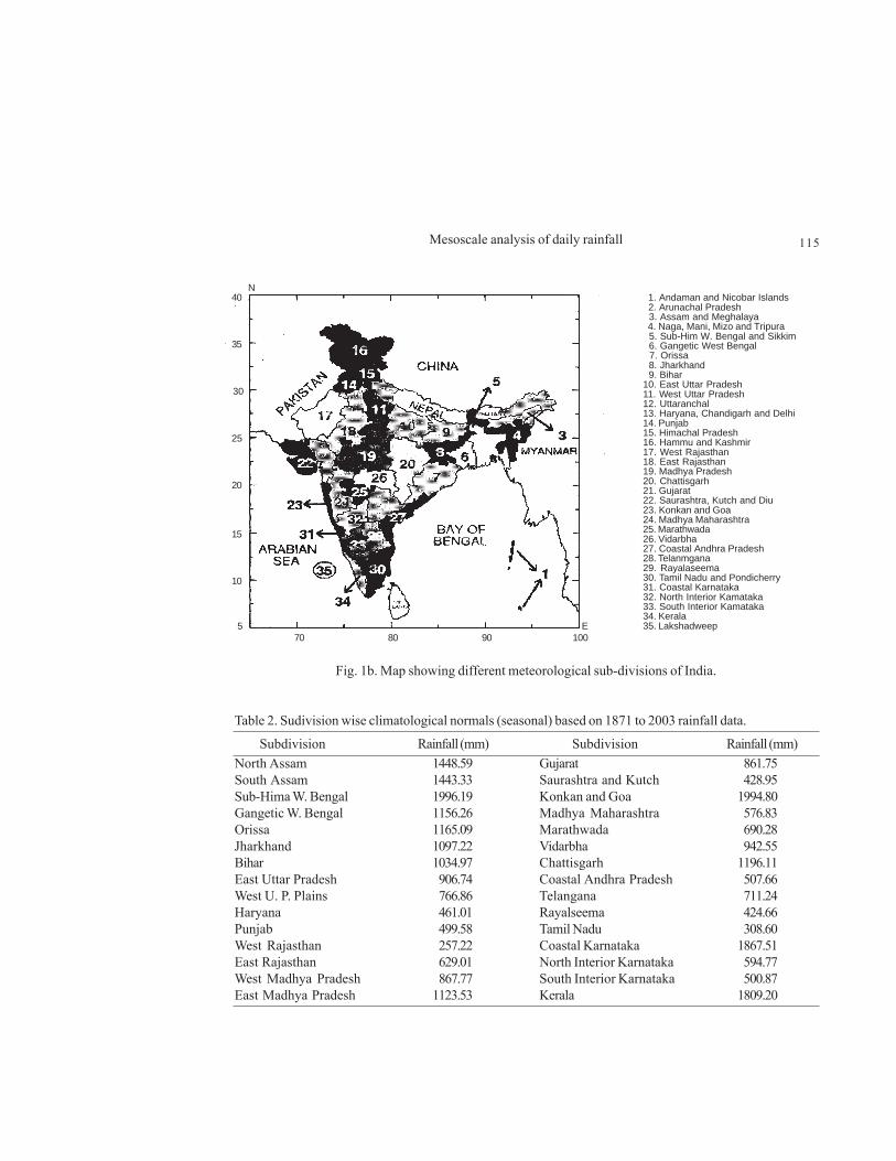
over Maharashtra are given in Table 1. Sub-division wise climatological normal rainfall valuesbased on 1871-2003 over India for the monsoon season (June-September) have been given in theTable 2 and the locations of different sub-division of India are shown in Figure 1b. This will help tounderstand the characteristics of rainfall over Indian region.

Fig. 1a. Locations of rainfallstations over Maharashtra.

22N

20N

18N

16N

72E 74E 76E 78E 80E

Maharashtra

Table 1. Latitude and longitude (degrees) for different observing stations over Maharashtra.

Station Lat. Long. Station Lat. Long. Station Lat. Long.

Achalapur 21.27 77.52 AheriTahs 19.40 80.00 AhmedpurT 18.70 76.93AiraTahsi 16.12 74.22 Akkalakot 17.53 76.20 Akkalkuwa 21.75 74.00AklujTahs 17.88 75.03 AkolaTahs 19.55 74.02 AkotTahsi 21.10 77.07AlibagTah 18.63 72.87 AmalnerTa 21.05 75.03 AmbadThas 19.62 75.80AmbegaonT 19.05 73.83 Ambejogai 18.73 76.38 AmravatiT 20.93 77.78Anjangaon 21.17 77.32 ArniTahsi 12.68 79.28 ArviTahsi 20.98 78.23AshitTahs 18.80 75.18 AshtiTahs 21.22 78.25 AsolaTahs 20.25 79.85Aurangaba 19.88 75.33 SataraTah 18.25 76.50 Babhulgao 20.38 78.13Badalkasa 21.37 80.05 BadneraTa 20.87 77.73 BalapurTa 20.67 76.78

Continues in the next page.


BaramatiI 18.15 74.58 Barshitak 20.50 77.10 BarshiTah 18.23 75.70BasmathTa 19.32 77.17 BeedIMDTa 19.00 75.77 BhadgaonT 20.67 75.23BhiraTahs 18.45 73.40 BhiwandiT 19.30 73.05 BhokarTah 19.22 77.68Bhokardan 20.25 75.77 BhorTahsi 18.13 73.85 Bramhapur 20.60 79.87BhusawalT 21.07 75.78 BiloliTah 18.77 77.73 BolthaneT 20.20 74.92BuldhanaT 20.53 76.18 Chalisgao 20.45 75.02 Chamorshi 19.95 79.90ChandagadT 15.93 74.18 ChandorTa 20.33 74.25 Chandrapu 19.95 79.95ChadurBa 21.25 77.73 ChandurRl 20.82 77.97 Chikaltha 19.85 75.40ChikhaliT 20.35 76.25 ChimurTah 20.50 79.38 ChiplunTa 17.53 73.52ChopdaTah 21.25 75.30 ChousalaT 18.72 75.70 DahanuTah 19.98 72.72DahiwadiT 17.70 74.55 DapoliTah 17.77 73.20 DaryapurT 20.93 77.33DeglurTah 18.55 77.58 DeogadTah 16.37 73.37 DeoliTahs 20.62 78.62DeoriTahs 21.07 80.37 DeorukhTa 17.05 73.62 DeolgaonR 20.03 76.03DhadgaonT 20.33 75.50 DharniTah 21.57 76.88 DharwhaTa 20.17 77.77DhondTahs 18.47 74.60 DhuleTahs 20.90 74.78 DigrasTah 20.12 77.72DindoriTa 20.20 73.83 EdlabadTa 21.07 76.07 ErandolTa 20.93 75.33Gadchirol 20.18 80.00 Gadhimgla 16.22 74.35 Gaganbava 16.55 73.83Gangakhed 18.92 76.75 GangapurT 19.68 75.02 GargoitBh 16.30 74.13GarmoshiT 19.95 79.90 GeoraiTah 19.25 75.75 Ghorazeri 20.53 79.63GuhagarTa 17.47 73.20 HadgaonTa 19.50 77.68 HarnaiIMD 17.82 73.10Hatkangal 16.75 74.43 Hingangha 20.55 78.83 HingoliTa 19.72 77.15IndapurTa 18.12 75.03 JalgaonJa 21.05 76.53 JalnaTahs 19.85 75.88JamkhedTa 18.73 75.32 JamnerTah 20.82 75.78 JawharTah 19.92 73.23JejuriTah 18.28 74.17 JinturTah 19.62 76.70 JunnerTah 19.22 73.88KagalTahs 16.58 74.32 nKalamKal 18.58 76.02 KalwanTah 20.50 74.03KalyanTah 19.25 73.12 KamteeTah 21.43 79.30 KandharTa 18.87 77.20Kanakavli 16.27 73.70 KannadTah 20.25 75.13 KaradTahs 17.28 74.18KaranjaTa 20.47 77.53 KarjatTah 18.55 75.00 KarmalaTa 18.40 75.20KarveerTa 16.70 74.23 KhamgaonT 20.72 76.57 KhandalaT 17.98 74.03KhariTahs 20.27 79.77 KhatavVad 17.60 73.40 KhedTahsi 17.72 73.40Khuldabad 20.00 78.20 Khyrband 21.48 80.07 KinwatTah 19.62 78.20KolegaonM 19.92 74.17 KolhapurI 16.70 74.23 Kopargaon 19.90 74.48KoregaonT 17.70 74.17 KotalTahs 21.27 78.58 KudalTahs 16.02 73.70KurkhedaT 19.58 79.83 LanjaTahs 16.87 73.55 LaturTahs 18.40 76.58LohaTahsi 19.08 77.33 LonarTahs 19.98 76.55 MadhaTahs 18.03 75.52MahadTahs 18.08 73.42 MalegaonT 20.55 74.53 MalsirasT 17.87 74.92MalwanMal 16.05 73.47 Mandangad 17.98 73.25 Mangalwed 17.50 75.45MangaonTa 18.23 73.28 Mangrulpi 20.32 77.35 Manjlegao 19.15 76.22MaregaonT 20.07 78.95 MatheranT 18.98 73.28 MavalTahs 18.73 73.65

Table 1. Latitude and longitude (degrees) for different observing stations over Maharashtra (continued).

Station Lat. Long. Station Lat. Long. Station Lat. Long.



MedhaTags 17.78 73.83 MehkarTah 20.17 76.55 MhasalaTa 18.13 73.12MhaswadTa 17.63 74.78 MohgaonTa 19.58 77.70 MoholTahs 17.82 75.65MokhadaTa 19.93 73.33 MorshiTah 21.33 78.02 MukhedTah 19.15 77.52MulTahsil 20.07 79.68 MurbadTah 19.40 73.40 Murtizapu 20.73 77.38MurudTahs 18.33 72.97 NagpurCit 21.15 79.12 NalesarTa 20.05 79.47NandedTah 19.13 77.33 NandgaonT 20.32 74.67 NanduraTa 20.83 76.47Nandurbar 21.33 74.25 NarkhedTa 21.45 78.53 NasikTahs 20.00 73.78NawapurTa 21.15 73.80 NerTahsil 20.48 77.87 NilangaTa 18.08 76.75NiphadTah 20.08 74.12 Osmanabad 18.17 76.05 PachoraTa 20.67 75.37PaithanTa 19.47 75.38 PalgharTa 19.65 72.72 Pandharka 20.02 78.55Pandharpu 17.65 75.33 PangriTah 21.42 80.10 PanhalaTa 16.80 74.12PanvelTah 18.98 73.12 PaoniTahs 20.78 79.65 ParandaTa 18.27 75.45ParbhaniI 19.27 76.77 ParnerTah 19.00 74.45 ParolaTah 20.88 75.12ParseoniT 21.37 79.15 ParturTah 19.58 76.22 PatanTahs 17.37 73.90PathardiT 19.17 75.17 PathriTah 19.25 76.43 PaturTahs 20.45 76.95PaudTahsi 18.53 73.62 PenTahsil 18.73 73.10 PhaltanTa 17.98 74.43Pimpalgao 20.17 73.98 Pimpalner 20.95 74.12 PoladpurT 17.92 73.42PotodaTah 18.80 75.48 PuneIMDTa 18.53 73.85 PusadTahs 19.92 77.58Radhanaga 16.33 73.98 RahuriTah 19.40 74.65 RajapurTa 16.65 73.52RajuraTah 19.77 79.37 RalegaonT 20.40 78.55 RamtekTah 21.40 79.33Ratnagiri 16.98 73.33 RaverTahs 21.25 75.03 RisodTahs 19.97 76.80RohaTahsi 18.43 73.12 RotiTahsi 18.80 75.12 SakoliTah 21.08 80.00SakriTahs 21.00 74.30 Sangamner 19.57 74.22 SangliIMD 16.87 74.57SangolaTa 17.43 75.20 SaonerTah 21.38 78.92 SaswadTah 18.35 74.03SatanaTah 20.60 74.20 SataraIMD 17.68 73.98 Sawantwad 15.90 73.82ShahadaTa 21.55 74.47 ShahapurT 19.45 73.33 Shahuwadi 16.88 74.00ShegaonTa 20.80 76.70 ShevgaonT 19.33 75.22 Shindkhed 21.28 74.75ShirolTah 16.74 74.60 ShirpurTa 21.35 74.88 Shrirampu 19.62 74.67Shriwardh 18.05 73.02 SillodTah 20.18 75.77 Sindewahi 20.28 79.68SinnerTah 19.85 74.00 SironchaT 18.83 79.97 SirurTahs 18.83 74.38SolapurTa 17.67 75.90 SomthaneT 19.93 74.23 SudhagadP 18.53 73.03SurganaTa 20.55 73.63 TalegaonT 18.65 74.15 TalodaTah 21.57 74.22TelharaTa 21.03 76.83 RisodTahs 19.97 76.80 ThaneTahs 19.20 72.98TiroraTir 21.43 79.93 TrimbakTa 19.95 73.53 TuljapurT 18.02 76.07TumsarTah 21.40 70.80 UdgirTahs 18.40 77.12 UmarkhedT 19.58 77.68UmrerTahs 20.85 79.33 UranTahsi 18.90 72.92 VadaTahsi 19.65 73.13VasaiTahs 19.35 72.80 VelheTahs 19.12 74.18 VengarlaT 15.87 73.63VaijapurT 19.93 74.73 Visarwadi 21.18 73.97 WaiTahsil 17.93 73.90WanawadiT 18.50 73.90 WaniTahsi 20.05 78.95 WardhaTah 20.75 78.60WaroraTah 20.22 79.02 WarudTahs 21.47 79.27 WashimTah 20.12 77.13YavalTahs 21.17 75.70 YeolaTahs 20.05 74.48 YeotmalTa 20.38 78.13

Table 1. Latitude and longitude (degrees) for different observing stations over Maharashtra (continued).Station Lat. Long. Station Lat. Long. Station Lat. Long.


1. Andaman and Nicobar Islands 2. Arunachal Pradesh 3. Assam and Meghalaya 4. Naga, Mani, Mizo and Tripura 5. Sub-Him W. Bengal and Sikkim 6. Gangetic West Bengal 7. Orissa 8. Jharkhand 9. Bihar10. East Uttar Pradesh11. West Uttar Pradesh12. Uttaranchal13. Haryana, Chandigarh and Delhi14. Punjab15. Himachal Pradesh16. Hammu and Kashmir17. West Rajasthan18. East Rajasthan19. Madhya Pradesh20. Chattisgarh21. Gujarat22. Saurashtra, Kutch and Diu23. Konkan and Goa24. Madhya Maharashtra25. Marathwada26. Vidarbha27. Coastal Andhra Pradesh28. Telanmgana29. Rayalaseema30. Tamil Nadu and Pondicherry31. Coastal Karnataka32. North Interior Kamataka33. South Interior Kamataka34. Kerala35. Lakshadweep

Fig. 1b. Map showing different meteorological sub-divisions of India.

40

35

30

N

25

20

15

10

70 80 90 1005 E

Table 2. Sudivision wise climatological normals (seasonal) based on 1871 to 2003 rainfall data.

Subdivision Rainfall (mm) Subdivision Rainfall (mm)North Assam 1448.59 Gujarat 861.75South Assam 1443.33 Saurashtra and Kutch 428.95Sub-Hima W. Bengal 1996.19 Konkan and Goa 1994.80Gangetic W. Bengal 1156.26 Madhya Maharashtra 576.83Orissa 1165.09 Marathwada 690.28Jharkhand 1097.22 Vidarbha 942.55Bihar 1034.97 Chattisgarh 1196.11East Uttar Pradesh 906.74 Coastal Andhra Pradesh 507.66West U. P. Plains 766.86 Telangana 711.24Haryana 461.01 Rayalseema 424.66Punjab 499.58 Tamil Nadu 308.60West Rajasthan 257.22 Coastal Karnataka 1867.51East Rajasthan 629.01 North Interior Karnataka 594.77West Madhya Pradesh 867.77 South Interior Karnataka 500.87East Madhya Pradesh 1123.53 Kerala 1809.20


3. MethodologyBarnes (1964, 1973) proposed an analysis scheme, which has probably replaced the Cressmananalysis scheme (1959). The Cressman scheme corrects the background grid point values by alinear combination of residuals between predicted and observed values. These residuals are thenweighted according to their distances from the grid point. The background field at each grid pointis successively adjusted on the basis of nearby observations in a series of scans (usually three tofour) through the data. The cutoff radius CR (the radius of the circle containing the observationswhich influence the correction) is reduced on successive scans in order to build smaller scaleinformation into the analyses where data density supports it. Cressman (1959) and Barnes (1973)objective analysis schemes are both weighted average techniques. One important difference isthe choice of cutoff radius CR. Cressman weights do not approach zero asymptotically withincreasing distance as they do in the Barnes technique, but instead abruptly become zero atdistance equal to CR. This aspect of the Cressman scheme causes a serious problem when thedata distribution is not uniform. The Barnes technique has gained wide importance in mesoscaleanalysis (e.g. Doswell, 1977; Maddox, 1980; Koch and McCarthy, 1982). This analysis producesa rainfall field on a regular grid from irregularly distributed observed rainfall stations. The rainfallestimated at a grid point ‘‘g’’ is a weighted average of surrounding observations, which areweighted according to the distance from the grid point. Achtemeier (1987) used a successivecorrection method so that an estimate of the rainfall fields is made on the first pass (iteration) andrefined on successive passes. Inner passes, which yield incremental changes to the initial rainfallfield, use shorter length scales so that relatively greater weight is assigned to observations closeto an analysis grid point.

The analysis is performed using Barnes two pass successive correction system (Barnes,1973; Koch et al., 1983). If a variable S(xm, ym) is observed at a location designated by m, then thefirst pass analysis at a grid point ‘‘g’’ is described by:

( )

∑

∑

=

== N

mm

mm

N

mm

g

w

yxSwS

1

11

,

(1)

⎟⎟⎠

⎞⎜⎜⎝

⎛ −= 2

2

expcdw m

m(2)

where the weight applied to the mth observation is given by:

The length scale c controls the rate of fall-off of the weighting function. Since the weightapproaches zero asymptotically, there is no need to specify a radius of influence. However, thenumber of observations N should be chosen large enough so that the observations far away from


the grid point receive a small weight. c exerts control over the filtering properties of the analysis.The analysis after the second pass is given by:

( ) ( )1

12 1

'

1

, ,N

m m m m mm

g g N

mm

'w s x y s x ys s

w

=

=

⎡ ⎤−⎣ ⎦= +

∑

∑(3)

⎟⎟⎠

⎞⎜⎜⎝

⎛ −= 2

2

expcdw m

m'

γ(4)

The analysis from the first pass provides a background field for the second pass. The weightsproduced by this function are in the range 0 to 1. γ is a numerical convergence parameter thatcontrols the difference between the weights on the first and second passes, and lies between 0 and1 (0 < γ < 1). Thus the weighting function has a steeper fall-off on the second pass in an attempt tobuild smaller scales into the analysis. Barnes (1964) objective analysis scheme without γ is convergent,but it requires several more passes to reach the same degree of convergence as compared toBarnes (1973) version with γ, which requires only two passes through the data.

A simple bilinear interpolation between the values of Sg1 at four surrounding grid points can be

used to obtain an estimate for s1(xm, ym) at each data location. If the average spacing of the dataand the grid points is small compared to some wavelength λ, then the representation of that wavelength(response function) after the second pass is given by (Barnes, 1973):

R = R0(1 + R0γ − 1 − Rγ

0)

where R0 = exp(− π 2 c2/λ2) is the response after the first pass. The response function R is themeasure of the degree of convergence after a second pass through the data. The shape of theresponse curve is illustrated in Figure 2.

4. Results and discussion4.1. Length scale and grid resolutionObjective determination of the analysis length scale (c) and grid resolution parameters (∆x) used inthe analysis scheme is made from the method of Koch et al. (1983). The choice of both parametersis based on the average station separation, ∆n and is given as:

∆n = √area/number of stations

where:

(5)


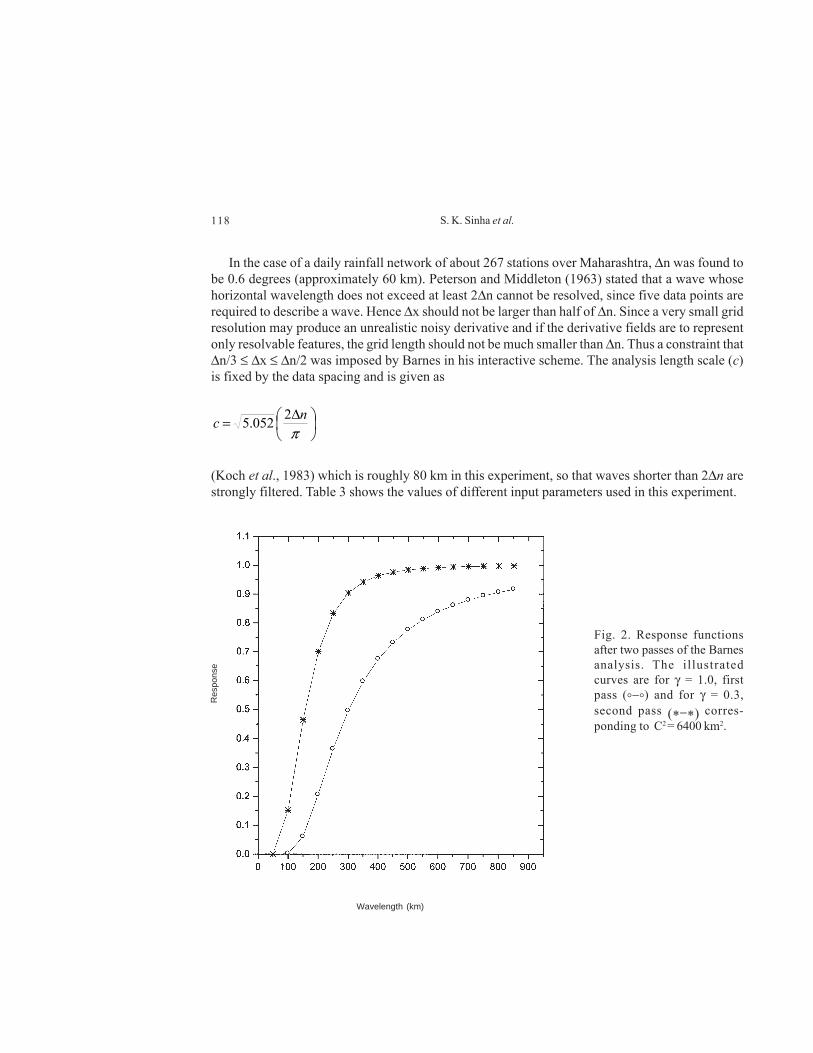
In the case of a daily rainfall network of about 267 stations over Maharashtra, ∆n was found tobe 0.6 degrees (approximately 60 km). Peterson and Middleton (1963) stated that a wave whosehorizontal wavelength does not exceed at least 2∆n cannot be resolved, since five data points arerequired to describe a wave. Hence ∆x should not be larger than half of ∆n. Since a very small gridresolution may produce an unrealistic noisy derivative and if the derivative fields are to representonly resolvable features, the grid length should not be much smaller than ∆n. Thus a constraint that∆n/3 ≤ ∆x ≤ ∆n/2 was imposed by Barnes in his interactive scheme. The analysis length scale (c)is fixed by the data spacing and is given as

Fig. 2. Response functionsafter two passes of the Barnesanalysis. The illustratedcurves are for γ = 1.0, firstpass (°−°) and for γ = 0.3,second pass (*−*) corres-ponding to C2 = 6400 km2.

⎟⎠⎞

⎜⎝⎛ ∆=

πnc 2052.5

Res

pons

e

Wavelength (km)

(Koch et al., 1983) which is roughly 80 km in this experiment, so that waves shorter than 2∆n arestrongly filtered. Table 3 shows the values of different input parameters used in this experiment.


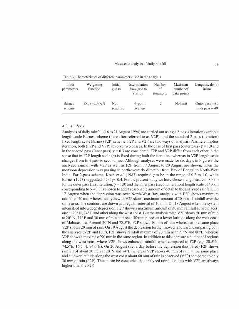
4.2. AnalysisAnalyses of daily rainfall (16 to 21 August 1994) are carried out using a 2-pass (iteration) variablelength scale Barnes scheme (here after referred to as V2P) and the standard 2-pass (iteration)fixed length scale Barnes (F2P) scheme. F2P and V2P are two ways of analysis. Pass here impliesiteration, both (F2P and V2P) involve two passes. In the case of first pass (outer pass) γ = 1.0 andin the second pass (inner pass) γ = 0.3 are considered. F2P and V2P differ from each other in thesense that in F2P length scale (c) is fixed during both the iterations whereas in V2P length scalechanges from first pass to second pass. Although analyses were made for six days, in Figure 3 theanalyzed rainfall with V2P as well as F2P from 17 August to 20 August are shown, when themonsoon depression was passing in north-westerly direction from Bay of Bengal to North-WestIndia. For 2-pass scheme, Koch et al. (1983) required γ to be in the range of 0.2 to 1.0, whileBarnes (1973) suggested 0.2 < γ < 0.4. For the present study we have chosen length scale of 80 kmfor the outer pass (first iteration, γ = 1.0) and the inner pass (second iteration) length scale of 40 kmcorresponding to γ = 0.3 is chosen to add a reasonable amount of detail to the analyzed rainfall. On17 August when the depression was over North-West Bay, analysis with F2P shows maximumrainfall of 40 mm whereas analysis with V2P shows maximum amount of 50 mm of rainfall over thesame area. The contours are drawn at a regular interval of 10 mm. On 18 August when the systemintensified into a deep depression, F2P shows a maximum amount of 30 mm rainfall at two places:one at 20° N, 74° E and other along the west coast. But the analysis with V2P shows 50 mm of rainat 20° N, 74° E and 30 mm of rain at three different places at a lower latitude along the west coastof Maharashtra. Around 20°N and 78.5°E, F2P shows 10 mm of rain whereas at the same placeV2P shows 20 mm of rain. On 19 August the depression further moved landward. Comparing boththe analyses (V2P and F2P), F2P shows rainfall maxima of 70 mm near 21°N and 80°E, whereasV2P shows a maxima of 90 mm in the same region. In addition to this there are a number of regionsalong the west coast where V2P shows enhanced rainfall when compared to F2P (e.g. 20.5°N,74.5°E; 16.5°N, 74.0°E). On 20 August (i.e. a day before the depression dissipated) F2P showsrainfall of about 20 mm at 20°N and 74°E, whereas V2P shows 40 mm of rain at the same placeand at lower latitude along the west coast about 60 mm of rain is observed (V2P) compared to only30 mm of rain (F2P). Thus it can be concluded that analyzed rainfall values with V2P are alwayshigher than the F2P.

Table 3. Characteristics of different parameters used in the analysis.

Input Weighting Initial Interpolation Number Maximum Length scale (c)parameters function guess from grid to of number of in km

station iterations data points

Barnes Exp (−dm2/γc2) Not 4−point 2 No limit Outer pass − 80

scheme required average Inner pass − 40


17.08.94

V2P F2P

Fig. 3. Objective analysis of August 17 and 18, 1994 with V2Pand F2P.


18.08.94


19.08.94

V2P F2P

Fig. 3. Objective analysis of August 19 and 20, 1994 with V2P and F2P (continued).

20.08.94


For the quantitative analysis of the rainfall root mean square (rms) errors for the six days arecomputed by comparing the analyzed rainfall against independent data not used in the analysis. Thisprocess is called cross validation approach and has been used widely dating back to Gandin (1963).That is, out of 267 observations 95% of data are used in the analysis and the verification is doneon the remaining 5%. In the verification the analyzed values have been interpolated to the observationlocations. The root mean squares (RMS) errors are generally between 8.15 to 16.58 mm for theV2P scheme, whereas for F2P they are in the range of 8.34 to 17.0 mm showing moderateimprovement of the V2P scheme over F2P. As the distribution of rainfall amounts is positivelyskewed (non-normal) and the rainfall is highly variable, the rms error can give a misleading pictureof rainfall analysis errors. This means a small number of large errors can unreasonably dominaterms statistics. Tapp et al. (1986) have shown that sometimes rms statistics on the cube root ofrainfall amounts (which are less skewed) can sometimes give a better picture of the analysis error.Often a mean absolute error is a more reasonable measure of rainfall analysis accuracy than rmserror. Table 4 shows the different types of errors and the standard deviations of rainfall on differentdays for the present study. It has been observed that when the standard deviation (SD) of theobserved rainfall values is high, on those days the rms errors of the analyzed rain are also high. Inmany cases, bias is a more important measure of analysis accuracy since the total rainfall over anarea, rather than the variation within the area, is often required from the analysis. Analyses basedon V2P have been found to be more accurate than analyses using F2P. The bias of the analysesbased on V2P is 2 % lower than that of analyses based on F2P.

Table 4. Analysis of errors for different days (mm) August 1994.

Scheme V2P F2P V2P F2P V2P F2P V2P F2P V2P F2P V2P F2P Date 16 17 18 19 20 21

RMS error 8.15 8.34 10.27 10.40 12.02 12.61 16.58 17.00 9.85 10.43 8.29 8.96RMS error of cubic 0.88 0.88 1.01 0.01 1.09 1.09 1.13 1.13 0.94 0.95 0.92 0.95root of rainfallMean absolute 4.43 4.62 6.52 6.80 8.69 9.23 12.31 13.04 7.10 7.62 6.10 6.65errorS D 9.70 12.25 13.24 19.97 12.44 9.63

In order to examine how the analysis changes with the variation of convergenceparameter (γ ), analysis with V1P (γ = 1.0, c = 80 km, Fig. 4a) and V2P (γ = 1.0, c =80 km; γ= 0.3, c = 40 km, Fig. 4b) are performed and displayed for 19 August. Figure 4b, which is forγ = 0.3, shows a rainfall maxima of 80 mm over northeast Maharashtra. But analysis with γ =1.0 (Fig.4a) shows maximum of 45 mm of rain over the same region. Also Figure 4a shows only 10 mmof rain over 20.5°N and 74.5°E whereas over the same region Figure 4b shows 40 mm of rain.At lower latitude along the west coast Figure 4a shows a maximum of 25 mm of rain but Figure 4bshows 40 to 60 mm of rain. Analysis of rainfall produced by V2P shows more number of maximawith lot of spatial variability, whereas analysis with V1P shows a very smooth distribution of rainfall.


Thus we find that analysis with V2P (γ = 0.3) produces superior. Figure 5a shows the analysis oftotal of six days (16 to 21 August) rainfall with V2P. Analyzed rain for the same period with F2P isshown in Figure 5b. Maximum rainfall of about 160 mm (F2P) is seen along the west coast (Fig.5b). But V2P (Fig. 5a) shows 150 to 200 mm of rain along the west coast. Contours are drawn atan interval of 20 mm. Average of daily rainfall (16 to 21 August 1994) at each grid point is computedfor both the analyses V2P as well as F2P and following Mills et al. (1997) analysis of the absolutedifference between the average daily rainfall fields in mm (V2P-F2P) is shown in Figure 6. Thus itcan be concluded that V2P produced a better analysis.

Fig. 4. Variation in the analysis with γ : (a) for γ = 1.0 and (b) for γ = 0.3 for 19 August 1994.(a) (b)

Fig. 5. Analysis of total rainfall (16-21 August 1994) with (a) V2P and (b) F2P.(a) (b)


Fig. 6. Analysis of absolutedifference between average dailystation rainfall (V2P-F2P).

5. ConclusionsNo worthwhile mesoscale research and modelling work can be carried out without good qualityof mesoscale data for the Indian region. The present study to analyze daily rainfall overMaharashtra is an effort in this direction. Daily rainfall analysis over Maharashtra has beenproduced using an interactive Barnes (1973) objective analysis scheme. Length scale and gridresolution are objectively determined from the average data spacing. Analyses with V2P as wellas F2P Barnes scheme have been performed to examine the performance of the two schemes.Length scale of 80 km corresponding to γ = 1.0 for the outer pass and length scale of 40 km forthe inner pass with γ = 0.3 are considered in this experiment.

It has been found that improvement in the analysis with V2P over F2P is moderate. Bias withV2P analysis is 2% less than F2P. Barnes (1994) has shown that analysis accuracy depends onthe regularity of observation spacing. He found that in an objective analysis based on 77 randomlydistributed observations mean absolute errors could be 40% higher than for an analysis based on23 uniformly distributed observations. Thus for producing better quality of rainfall analysis werequire more uniformly distributed rainfall observations. This scheme has the following advantages.

(i) There is no need to specify an influence radius.(ii) Two to three passes are required to reach convergence.(iii) Background field (first guess) is not required. Therefore analysis can be performed without

the use of a model.Objective analyses for the six-day period were made using two passes (γ = 1.0 and γ = 0.3).

Errors were computed by comparing the analyses with the observations using a cross validationtechnique. Mesoscale analysis involves assimilation of data from different sources and sensors.Plans are ahead to include satellite data to complement the existing raingauge data and the length


scale used in this study can then be adjusted accordingly. Satellite data will also extend the analysisarea over oceans and also over data sparse regions. Our main task is to combine optimally theraingauge data with data from other sources. Currently we are in the process of analyzing dailyrainfall for longer periods over a larger region (whole India) and with number of different synopticsituations.

AcknowledgementsThe authors are extremely grateful to Dr. G. B. Pant, Director, Indian Institute of Tropical Meteorology,Pune, for the necessary facilities. We are thankful to Shri P. Seetaramayya, Head, FRD for hisencouragement. We also express our gratitude to the anonymous referees for the constructivecomments and suggestions. Thanks are also due to India Meteorological Department and theAgriculture Department of Government of Maharashtra for providing us with the rainfall data. Lastbut not least we extend our thanks to Miss Anindita for her technical support.

ReferencesAchtemeier G. L., 1987. On the concept of varying influence radii for a successive corrections

objective analysis. Mon. Wea. Rev. 115, 1760-1771.Barnes S. L., 1964. A technique for maximizing details in a numerical weather map analysis. J.

Appl. Meteorol. 3, 396-409.Barnes S. L., 1973. Mesoscale objective map analysis using weighted time-series observations. NOAA Tech. Memo. ERL NSSL-62, National Severe Storms Laboratory, Norman, OK 73069,

60 pp. [NTIS COM-73-10781].Barnes S. L., 1994. Applications of the Barnes objective analysis scheme. Part I: Effects of

undersampling, wave position and station randomness. J. Atmos. Oceanic Tech. 11, 1433-1448.Bussieres N. and W. Hogg, 1989. The objective analysis of daily rainfall by distance weighting

schemes on a mesoscale grid. Atmosphere-Ocean. 27, 521-541.Cressman G. P., 1959. An operational objective analysis system. Mon. Wea. Rev. 87, 367-374.Das P. K., 1986. Monsoons. WMO monograph No. 613, WMO, Geneva, 155 pp.Doswell C. A., 1977. Obtaining meteorologically significant surface divergence fields through the filtering property of objective analysis. Mon. Wea. Rev. 105, 885-892.Gandin L. S., 1963. Objective analysis of meteorological fields (in Russian). Israel Program for

Scientific Translation. 242 pp.India Meteorological Department, 1981. Climatological atlas of India. Part I: Rainfall, New Delhi,

69 charts.Koch S. E. and J. McCarthy, 1982. The evolution of an Oklahoma dry line. Part II Boundary-layer

forcing of mesoconvective systems. Mon. Wea. Rev. 39, 237-257.Koch S. E., M. desJardins and P. J. Kocin, 1983. An interactive Barnes objective map analysis

scheme for use with satellite and conventional data. J. Clim. Appl. Meteorol. 22, 1487-1503.


Maddox R. A., 1980. An objective technique for separating macroscale and mesoscale features inmeteorological data. Mon. Wea. Rev. 108, 1108-1121.

Mills G. A., G. Weymouth, D. Jones, E. E. Ebert, M. Manton, J. Lorkin and J. Kelly, 1997. ANational objective daily rainfall analysis system. BMRC Techniques Development Report No.130 pp.

Mitra A. K., A. K. Bohra and D. Rajan, 1997. Daily rainfall analysis for Indian summer monsoon region. Int. J. Clim. 17, 1083-1092.Mooley D. A., 1973. Some aspects of Indian monsoon depressions and associated rainfall. Mon.

Wea. Rev. 101, 271-280.Peterson D. P. and D. Middleton, 1963. On representative observations. Tellus 15, 387-405.Raddatz R. L., 1987. Mesoscale representativeness of rainfall measurements for Winnipeg.

Atmosphere- Ocean, 25, 267-278.Rao K. N., C. J. George and V. P. Abhyankar, 1971. Nature of the frequency distribution of Indian rainfall (monsoon and annual). Rep. No. 168, India Meteorological Department, Pune, India.

on a mesoscale grid

Documents