Oil Price Elasticities and Oil Price Fluctuations ∗

Dario Caldara1, Michele Cavallo2, and Matteo Iacoviello†3

1Federal Reserve Board2Federal Reserve Board3Federal Reserve Board

July 16, 2018

Abstract

Studies identifying oil shocks using structural vector autoregressions (VARs) reach

different conclusions on the relative importance of supply and demand factors in explaining

oil market fluctuations. This disagreement is due to different assumptions on the oil supply

and demand elasticities that determine the identification of the oil shocks. We provide

new estimates of oil-market elasticities by combining a narrative analysis of episodes of

large drops in oil production with country-level instrumental variable regressions. When

the estimated elasticities are embedded into a structural VAR, supply and demand shocks

play an equally important role in explaining oil prices and oil quantities.

KEYWORDS: Oil Market; Oil Elasticity; Vector Autoregressions; Narrative Analysis; Instru-

mental Variables.

JEL CLASSIFICATION: Q43. C32. E32. F50.

∗The authors thank Soojin Jo and Martin Stuermer for their thoughtful discussions, seminar participantsat EIEF and the Federal Reserve Board, conference participants at the EIA, the Bank of Canada, the FederalReserve SCIEA and System Energy Meetings, the IAAE meetings in Thessaloniki and Milan, the LACEAmeeting in Santa Cruz, Bolivia, and the CEF meeting in Bordeaux for feedback. Michelle Bongard, KhalelaFrancis, Lucas Husted and J Seymour provided outstanding research assistance. The views expressed in thispaper are solely the responsibility of the authors and should not be interpreted as reflecting the views of theBoard of Governors of the Federal Reserve System or of anyone else associated with the Federal Reserve System.†Corresponding author: Division of International Finance, Federal Reserve Board, 20th and C St. NW,

20551, Washington, DC United States. E-mail:matteo.iacoviello@frb.gov.

1 Introduction

Academics, practitioners, and policymakers attribute swings in the price of oil to a variety of

forces, such as changes in global demand, disruptions in supply, and precautionary motives.

However, the relative importance of these forces remains highly debated. In their chapter in

the Handbook of Macroeconomics, Stock and Watson (2016) summarize the academic debate

by comparing an early literature that finds an important role for oil supply shocks in driving

oil market fluctuations to a more recent literature that finds that most movements in oil prices

are demand-driven.1

In this paper, we assess the relative importance of supply and demand factors in explaining

oil market fluctuations, and find that supply and demand shocks are equally important in

accounting for fluctuations in oil prices and oil quantities. We reach this conclusion in two

steps. First, we combine narrative analysis with a panel of observations on country-specific

oil production and consumption to estimate oil supply and demand elasticities. Second, we

embed these elasticities in a vector autoregression (VAR) to identify the oil supply and demand

equations and, consequently, the associated oil supply and oil demand shocks.

Our starting point is to show how the cross-equation restrictions that are inherent in stan-

dard VARs of the oil market impose an inverse, nonlinear relation between the short-run price

elasticities of oil supply and demand. This relation—as originally noted by Baumeister and

Hamilton (2017)— implies that seemingly plausible restrictions on the oil supply elasticity may

map onto implausible values of the oil demand elasticity, and vice versa. For instance, if one

imposes a short-run oil supply elasticity of zero, a common value in the literature, the resulting

oil demand elasticity is −1, a value which is in the high end of the empirical estimates.2 Simi-

1The early literature, initially used to study the 1970s oil shocks, assumes that oil prices are predetermined,and interprets innovations in prices as the outcome of oil supply shocks. Examples of papers adopting thisapproach are Shapiro and Watson (1988), Rotemberg and Woodford (1996), and Blanchard and Galı (2010).Blanchard and Galı (2010) identify an oil shock that explains about 80 percent of oil prices, and interpret theshock as being mostly driven by oil supply factors. The more recent literature, promoted by Kilian (2009),assumes that the short-run oil supply elasticity is zero, and explicitly allows for oil prices to contemporaneouslyrespond to movements in oil production and in global demand. This literature finds that oil-specific demandshocks are important drivers of oil prices.

2See Hamilton (2009) for a survey of the estimates of the short-run price elasticity of demand for crude oil:the average estimate of the demand elasticity is −0.06.

2

larly, if one imposes an oil demand elasticity of −0.05, a value in the ballpark of the empirical

estimates, the resulting supply elasticity is large, close to 0.5.

We next argue that the selection of the elasticities is essential for understanding sources and

consequences of oil market fluctuations, and that seemingly small changes in these elasticities

have large effects on the relative importance of demand and supply forces. In particular, with

a configuration of the oil market characterized by a zero supply elasticity, all movements in oil

prices are attributed to oil-specific demand shocks. By contrast, setting the supply elasticity

to 0.1 implies that oil supply and oil demand shocks are equally important drivers of oil price

fluctuations.

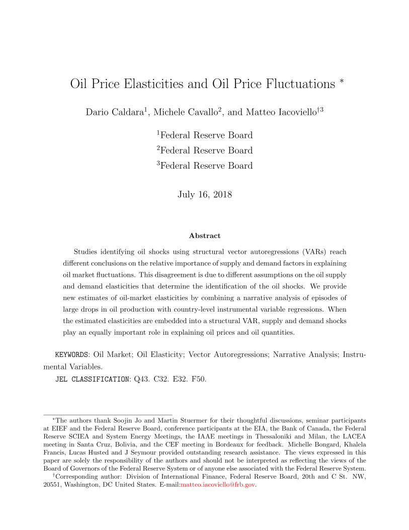
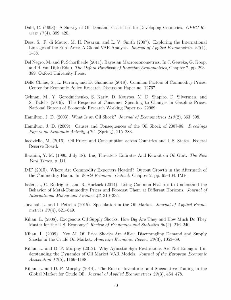
To understand the relationship between oil price elasticities and oil price fluctuations, Fig-

ure 1 shows a scatter plot between monthly surprises in oil prices and global oil production

implied by simple univariate AR(1) regressions.3 The dots show that oil prices and global oil

production are uncorrelated. This lack of correlation could be the outcome of very different

oil market configurations. On one hand, as shown by the dashed lines in Figure 1, the supply

curve could be inelastic, while the demand curve could be very elastic. As a result, fluctuations

in oil prices and oil production would be disconnected, with prices driven uniquely by demand

shocks, and production driven uniquely by supply shocks. On the other hand, a market char-

acterized by a very elastic oil supply curve and an inelastic demand curve—the dotted lines

in Figure 1—would also lead to a disconnect of movements in oil prices and oil production.

In between these two extremes lies an oil market with a downward-sloping demand curve and

an upward-sloping supply curve—the solid lines in Figure 1—which would imply that demand

and supply shocks jointly affect oil prices and production. These market configurations, picked

among many for illustrative purposes, are equally consistent with the data but have different

implications for the causes and the consequences of oil price fluctuations.

In order to estimate oil supply and demand elasticities, we combine narrative analysis with

instrumental-variable regressions for a large panel of countries. For each country, we instrument

3A similar figure would obtain by plotting the reduced-form residuals for oil prices and oil productionestimated using a VAR.

3

the price of oil with large, exogenous drops in oil production occurring in other countries.

This approach yields a supply elasticity of 0.08, and a demand elasticity of −0.08. These

estimated elasticities are used as external information to identify the structural shocks in our

VAR. In particular, we propose an identification scheme that minimizes the distance between

the elasticities consistent with the cross-equation restrictions of the VAR, and the elasticities

using external information. In doing so, we derive VAR-consistent elasticities of 0.10 for supply,

and of −0.14 for demand.

Even with this identification strategy in hand, an additional challenge is to disentangle

demand shocks that are specific to the oil market from demand shocks that originate from

changes in global economic activity. To this end, we use three indicators of global activity

that provide a broad characterization of the global demand for oil. We construct two separate

indicators based on industrial production, one for emerging economies, and another for advanced

economies, dating back to the mid 1980s. These indicators allow us to measure the distinct

consequences of oil shocks on advanced versus emerging economies in a parsimonious model.

Our third indicator is an index of industrial metal prices, which are often viewed by policymakers

and practitioners as leading indicators of swings in economic activity and global risk sentiment.4

Our analysis delivers the following results. First, oil supply shocks are the main driving

force of oil market movements, accounting for about 35 percent of the volatility of oil prices,

and about 45 percent of the volatility of oil production. Shocks to global economic conditions

also play an important role, explaining 35 percent of the volatility of oil prices, and about

20 percent of the volatility of oil production. Second, a drop in oil prices driven by either oil

demand or supply shocks depresses economic activity in emerging economies. A drop in oil

prices boosts economic activity in advanced economies only when driven by supply shocks.

4The use of IP indicators for advanced and emerging countries to measure global activity hews closely to thework of Baumeister and Hamilton (2017) and Aastveit et al. (2015). The use of metal prices follows the lead ofBarsky and Kilian (2001), who propose the use of an index of industrial commodity prices—excluding oil—toidentify broad-based shifts in global demand, as well as the more recent work of Arezki and Blanchard (2014),who exploit the idea that metal prices typically react to global activity even more than oil prices. Other studiesthat find a meaningful link between cyclical fluctuations in global economic activity and movements in metalprices include Pindyck and Rotemberg (1990), Labys et al. (1999), Cuddington and Jerrett (2008), Lombardiet al. (2012), Issler et al. (2014), Delle Chiaie et al. (2018), and Stuermer (2018).

4

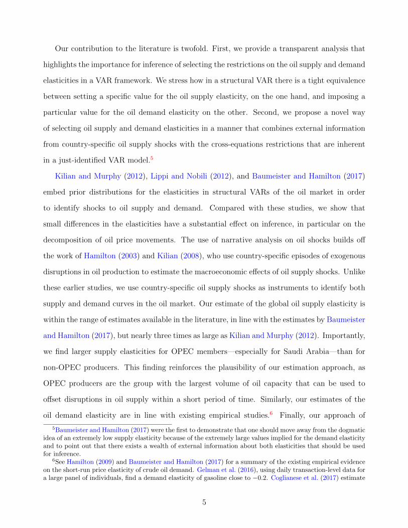
Our contribution to the literature is twofold. First, we provide a transparent analysis that

highlights the importance for inference of selecting the restrictions on the oil supply and demand

elasticities in a VAR framework. We stress how in a structural VAR there is a tight equivalence

between setting a specific value for the oil supply elasticity, on the one hand, and imposing a

particular value for the oil demand elasticity on the other. Second, we propose a novel way

of selecting oil supply and demand elasticities in a manner that combines external information

from country-specific oil supply shocks with the cross-equations restrictions that are inherent

in a just-identified VAR model.5

Kilian and Murphy (2012), Lippi and Nobili (2012), and Baumeister and Hamilton (2017)

embed prior distributions for the elasticities in structural VARs of the oil market in order

to identify shocks to oil supply and demand. Compared with these studies, we show that

small differences in the elasticities have a substantial effect on inference, in particular on the

decomposition of oil price movements. The use of narrative analysis on oil shocks builds off

the work of Hamilton (2003) and Kilian (2008), who use country-specific episodes of exogenous

disruptions in oil production to estimate the macroeconomic effects of oil supply shocks. Unlike

these earlier studies, we use country-specific oil supply shocks as instruments to identify both

supply and demand curves in the oil market. Our estimate of the global oil supply elasticity is

within the range of estimates available in the literature, in line with the estimates by Baumeister

and Hamilton (2017), but nearly three times as large as Kilian and Murphy (2012). Importantly,

we find larger supply elasticities for OPEC members—especially for Saudi Arabia—than for

non-OPEC producers. This finding reinforces the plausibility of our estimation approach, as

OPEC producers are the group with the largest volume of oil capacity that can be used to

offset disruptions in oil supply within a short period of time. Similarly, our estimates of the

oil demand elasticity are in line with existing empirical studies.6 Finally, our approach of

5Baumeister and Hamilton (2017) were the first to demonstrate that one should move away from the dogmaticidea of an extremely low supply elasticity because of the extremely large values implied for the demand elasticityand to point out that there exists a wealth of external information about both elasticities that should be usedfor inference.

6See Hamilton (2009) and Baumeister and Hamilton (2017) for a summary of the existing empirical evidenceon the short-run price elasticity of crude oil demand. Gelman et al. (2016), using daily transaction-level data fora large panel of individuals, find a demand elasticity of gasoline close to −0.2. Coglianese et al. (2017) estimate

5

combining country-specific data on oil production with an aggregate VAR echoes the approach

of the global VAR (GVAR) literature pioneered by Dees et al. (2007), and Mohaddes and

Pesaran (2016).

2 Identifying Oil Market and Global Activity Shocks

2.1 Model Overview

The structure describing the oil market and its relationship with the global economy is given

by the following structural VAR:

AXt =

p∑j=1

αjXt−j + ut, (1)

where X is a vector of oil–market and macroeconomic variables, ut is the vector of structural

shocks, p is the lag length, and A and αj for j = 1, ..., p are matrices of structural parame-

ters. The vector ut is assumed to have a Gaussian distribution with zero mean and variance–

covariance matrix E [utu′t] = Σu. Without loss of generality, we normalize one entry on each

row of A to 1 and we assume that Σu is a diagonal matrix. The reduced-form representation

for Xt is the following:

Xt =

p∑j=1

γjXt−j + εt, (2)

where the reduced-form residuals εt are related to the structural shocks ut as follows:

εt = But, (3)

Σε = BΣuB′, (4)

where B = A−1, so that ut can be alternatively expressed as ut = Aεt. Estimation of the

reduced-form VAR allows us to obtain a consistent estimate of the n (n+ 1) /2 distinct entries

an elasticity of gasoline demand of −0.37 that is not statistically significant. As discussed in Hamilton (2009),since crude oil represents about half of the retail cost of gasoline, the price elasticity of demand for crude oilshould be about half of that for retail gasoline.

6

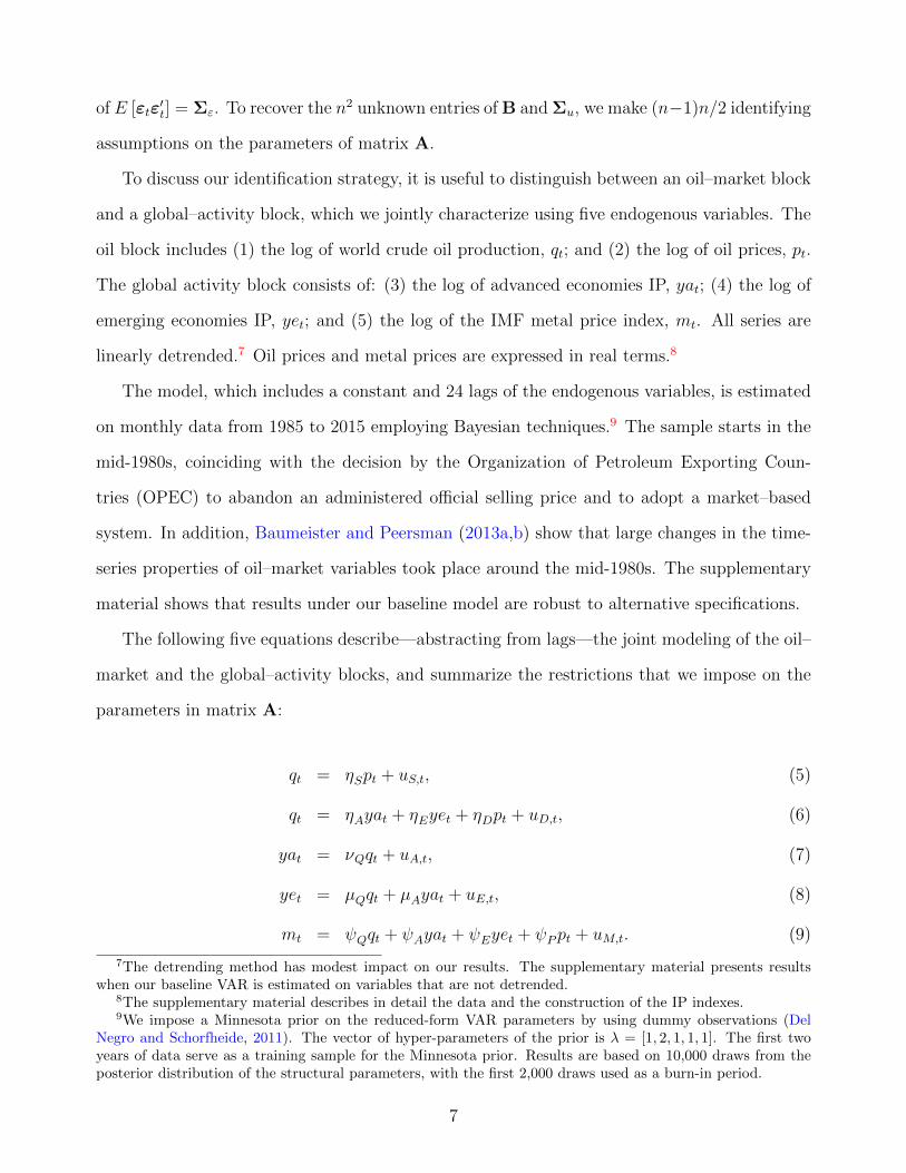
of E [εtε′t] = Σε. To recover the n2 unknown entries of B and Σu, we make (n−1)n/2 identifying

assumptions on the parameters of matrix A.

To discuss our identification strategy, it is useful to distinguish between an oil–market block

and a global–activity block, which we jointly characterize using five endogenous variables. The

oil block includes (1) the log of world crude oil production, qt; and (2) the log of oil prices, pt.

The global activity block consists of: (3) the log of advanced economies IP, yat; (4) the log of

emerging economies IP, yet; and (5) the log of the IMF metal price index, mt. All series are

linearly detrended.7 Oil prices and metal prices are expressed in real terms.8

The model, which includes a constant and 24 lags of the endogenous variables, is estimated

on monthly data from 1985 to 2015 employing Bayesian techniques.9 The sample starts in the

mid-1980s, coinciding with the decision by the Organization of Petroleum Exporting Coun-

tries (OPEC) to abandon an administered official selling price and to adopt a market–based

system. In addition, Baumeister and Peersman (2013a,b) show that large changes in the time-

series properties of oil–market variables took place around the mid-1980s. The supplementary

material shows that results under our baseline model are robust to alternative specifications.

The following five equations describe—abstracting from lags—the joint modeling of the oil–

market and the global–activity blocks, and summarize the restrictions that we impose on the

parameters in matrix A:

qt = ηSpt + uS,t, (5)

qt = ηAyat + ηEyet + ηDpt + uD,t, (6)

yat = νQqt + uA,t, (7)

yet = µQqt + µAyat + uE,t, (8)

mt = ψQqt + ψAyat + ψEyet + ψPpt + uM,t. (9)

7The detrending method has modest impact on our results. The supplementary material presents resultswhen our baseline VAR is estimated on variables that are not detrended.

8The supplementary material describes in detail the data and the construction of the IP indexes.9We impose a Minnesota prior on the reduced-form VAR parameters by using dummy observations (Del

Negro and Schorfheide, 2011). The vector of hyper-parameters of the prior is λ = [1, 2, 1, 1, 1]. The first twoyears of data serve as a training sample for the Minnesota prior. Results are based on 10,000 draws from theposterior distribution of the structural parameters, with the first 2,000 draws used as a burn-in period.

7

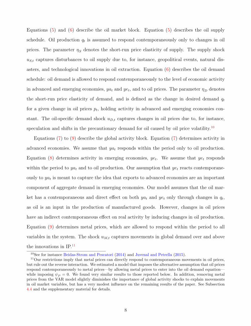
Equations (5) and (6) describe the oil market block. Equation (5) describes the oil supply

schedule. Oil production qt is assumed to respond contemporaneously only to changes in oil

prices. The parameter ηS denotes the short-run price elasticity of supply. The supply shock

uS,t captures disturbances to oil supply due to, for instance, geopolitical events, natural dis-

asters, and technological innovations in oil extraction. Equation (6) describes the oil demand

schedule: oil demand is allowed to respond contemporaneously to the level of economic activity

in advanced and emerging economies, yat and yet, and to oil prices. The parameter ηD denotes

the short-run price elasticity of demand, and is defined as the change in desired demand qt

for a given change in oil prices pt, holding activity in advanced and emerging economies con-

stant. The oil-specific demand shock uD,t captures changes in oil prices due to, for instance,

speculation and shifts in the precautionary demand for oil caused by oil price volatility.10

Equations (7) to (9) describe the global activity block. Equation (7) determines activity in

advanced economies. We assume that yat responds within the period only to oil production.

Equation (8) determines activity in emerging economies, yet. We assume that yet responds

within the period to yat and to oil production. Our assumption that yet reacts contemporane-

ously to yat is meant to capture the idea that exports to advanced economies are an important

component of aggregate demand in emerging economies. Our model assumes that the oil mar-

ket has a contemporaneous and direct effect on both yat and yet only through changes in qt,

as oil is an input in the production of manufactured goods. However, changes in oil prices

have an indirect contemporaneous effect on real activity by inducing changes in oil production.

Equation (9) determines metal prices, which are allowed to respond within the period to all

variables in the system. The shock uM,t captures movements in global demand over and above

the innovations in IP.11

10See for instance Beidas-Strom and Pescatori (2014) and Juvenal and Petrella (2015).11Our restrictions imply that metal prices can directly respond to contemporaneous movements in oil prices,

but rule out the reverse interaction. We estimated a model that imposes the alternative assumption that oil pricesrespond contemporaneously to metal prices—by allowing metal prices to enter into the oil demand equation—while imposing ψP = 0. We found very similar results to those reported below. In addition, removing metalprices from the VAR model slightly diminishes the importance of global activity shocks to explain movementsin oil market variables, but has a very modest influence on the remaining results of the paper. See Subsection4.4 and the supplementary material for details.

8

The use of zero restrictions to model the interaction between the oil market and global

activity is consistent with the assumptions in Kilian (2009), who also assumes that oil supply

does not respond to shocks to global activity, while oil demand does. The key difference between

Kilian’s (2009) identification strategy and ours lies in the choice of the oil supply and demand

elasticities ηS and ηD.

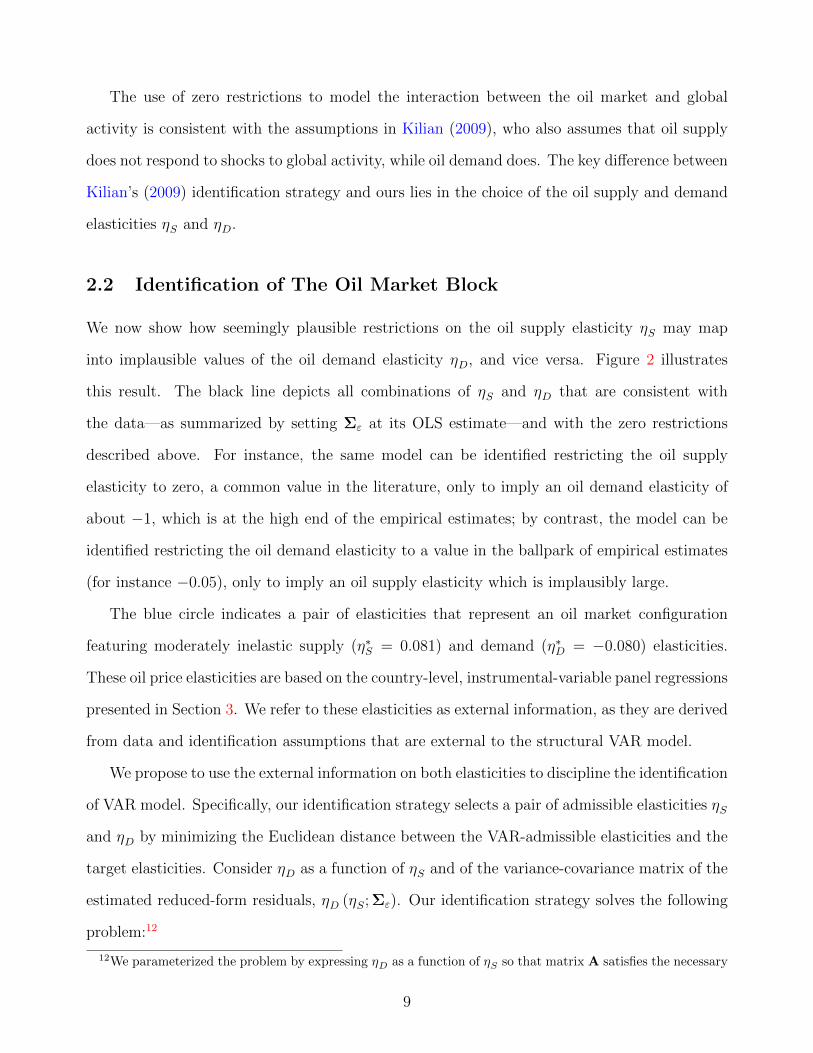
2.2 Identification of The Oil Market Block

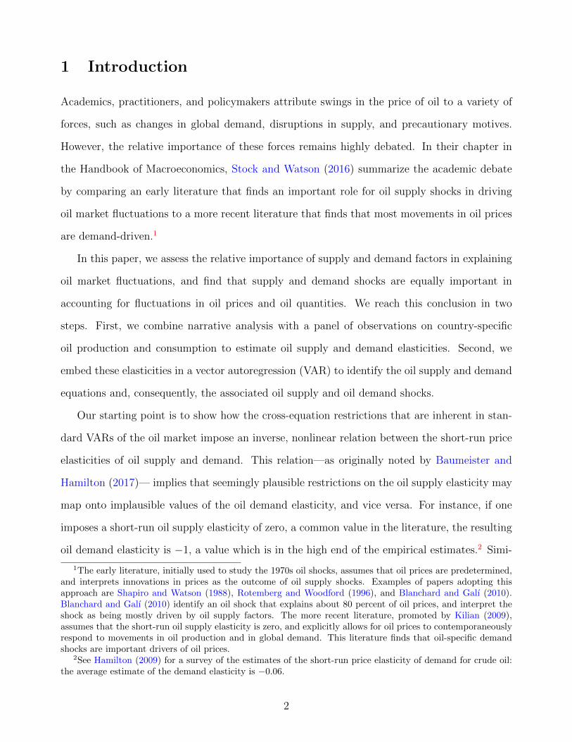
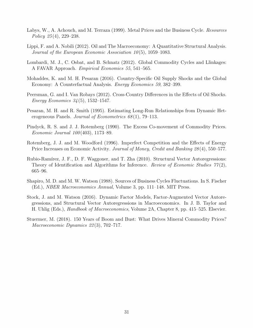
We now show how seemingly plausible restrictions on the oil supply elasticity ηS may map

into implausible values of the oil demand elasticity ηD, and vice versa. Figure 2 illustrates

this result. The black line depicts all combinations of ηS and ηD that are consistent with

the data—as summarized by setting Σε at its OLS estimate—and with the zero restrictions

described above. For instance, the same model can be identified restricting the oil supply

elasticity to zero, a common value in the literature, only to imply an oil demand elasticity of

about −1, which is at the high end of the empirical estimates; by contrast, the model can be

identified restricting the oil demand elasticity to a value in the ballpark of empirical estimates

(for instance −0.05), only to imply an oil supply elasticity which is implausibly large.

The blue circle indicates a pair of elasticities that represent an oil market configuration

featuring moderately inelastic supply (η∗S = 0.081) and demand (η∗D = −0.080) elasticities.

These oil price elasticities are based on the country-level, instrumental-variable panel regressions

presented in Section 3. We refer to these elasticities as external information, as they are derived

from data and identification assumptions that are external to the structural VAR model.

We propose to use the external information on both elasticities to discipline the identification

of VAR model. Specifically, our identification strategy selects a pair of admissible elasticities ηS

and ηD by minimizing the Euclidean distance between the VAR-admissible elasticities and the

target elasticities. Consider ηD as a function of ηS and of the variance-covariance matrix of the

estimated reduced-form residuals, ηD (ηS; Σε). Our identification strategy solves the following

problem:12

12We parameterized the problem by expressing ηD as a function of ηS so that matrix A satisfies the necessary

9

minηS

ηS − η∗S

ηD (ηS; Σε)− η∗D

V −1 ηS − η∗S

ηD (ηS; Σε)− η∗D

, (10)

where η∗S and η∗D are the target values for the supply and demand elasticities, respectively,

and V is a diagonal matrix of weights. We summarize the external information into a mean

component, the targets η∗S and η∗D, and into a variance component, which we use to calibrate

the weights V. If the external information is perfectly consistent with the VAR, η∗S and η∗D are

on the curve plotted in Figure 2 and the distance between the VAR-implied elasticities and the

targets is zero. By contrast, if the external information is not consistent with the VAR, η∗S and

η∗D are not on the curve and the identification selects the pair of elasticities on the curve that

are as close as possible to the targets, assigning a larger weight to the elasticity that is more

precisely estimated.

In our application, the identification selects ηS = 0.10 and ηD = −0.14, denoted by the

green square in Figure 2. Both values are close to their target.

In sum, standard VAR models of the oil market face a trade–off in the selection of the oil

supply and demand elasticities. For instance, the same model can be identified restricting the

oil supply elasticity to using a common value in the literature (for instance 0), only to imply an

oil demand elasticity which is at the high end of the empirical estimates; by contrast, the model

can be identified restricting the oil demand elasticity to a value in the ballpark of empirical

estimates (for instance −0.05), only to imply an oil supply elasticity which is implausibly

large. Our approach eases this potential tension by making use of external information on both

elasticities to select a model with oil elasticities that are as close as possible to empirically

plausible values.

and sufficient conditions for identification of Rubio-Ramırez et al. (2010). Thus, the structural parameters(νQ, µQ, µA, ηA, ηE , ηD, ψQ, ψA, ψE , ψP ,Σu

)are uniquely identified given information from Σε.

10

2.3 The Role of Oil Demand and Oil Supply Elasticities

One could argue that an oil supply elasticity of, say, 0.01 is not meaningfully different from an

elasticity of, say, 0.05. In this subsection, we show that this is not the case. Small changes in

the oil price elasticities have large and material implications for quantifying the determinants

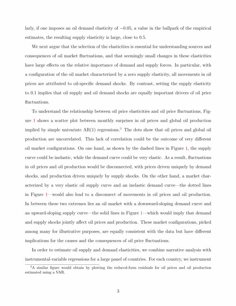
of fluctuations in oil prices and oil production. Figure 3 illustrates this result by plotting—for

our baseline model—the share of the forecast error variance at horizon zero for oil prices and

for oil production that is attributable to oil shocks, as a function of the oil supply elasticity ηS.

Consider the case in which the supply elasticity is assumed to be zero, the value used in

Kilian (2009). By assumption, setting a zero supply elasticity implies that oil production is

exogenous within the month, as the supply curve is perfectly inelastic. Accordingly, as shown

by the red line in the right panel of Figure 3, all of its forecast error variance is accounted for

by the oil supply shock. However, an additional implication of setting a zero supply elasticity

is that, as shown in the left panel, almost all of the forecast error variance of oil prices—about

95 percent—is explained by the oil-specific demand shock. This is due to the fact that the

demand curve implied by the VAR is highly elastic. Thus, setting ηS = 0 implies a disconnect

between the drivers of oil production and the drivers of oil prices: oil production moves in

response to shocks to oil supply, whereas oil prices move in response to shocks to oil demand.

Figure 3 also shows that small variations in the oil supply elasticity significantly alter the

relative importance of oil-specific supply and demand shocks in accounting for fluctuations in the

price of oil. In particular, a value of ηS close to 0.1, similar to that selected by our identification

strategy, implies that the two shocks are equal drivers of oil prices and oil production. Thus,

for sufficiently upward-sloping supply curves and sufficiently downward-sloping demand curves,

the two oil shocks jointly affect oil prices and production, and there is no disconnect between

drivers of oil production and drivers of oil prices.13

13The supplementary material places our identification strategy in the context of the old and new VARliterature—surveyed in Stock and Watson (2016)—studying the macroeconomic effects of oil shocks.

11

3 IV Estimates of Oil Supply and Demand Elasticities

This section provides empirical evidence about the price elasticity of global supply and demand

for crude oil by estimating instrumental variable (IV) panel regressions. This evidence provides

the basis for the target elasticities that we impose to identify the structural VAR.

3.1 A Stylized Model of the Global Oil Market

Our starting point is a small, stylized empirical model that provides the basis for estimating oil

supply and oil demand elasticities starting from individual countries’ oil production data. The

empirical model posits that the global oil market consists of N countries, and has the following

structure:

∆qS,i,t = ηS∆pt + uS,i,t, ∀i = 1, ..., n, (11)

∆qD,i,t = ηD∆pt + uD,i,t,∀i = 1, ..., n, (12)N∑i=1

ωS,i∆qS,i,t =N∑i=1

ωD,i∆qD,i,t. (13)

Equation (11) is the oil supply schedule in country i. According to this equation, the log change

in country i’s production of crude oil (∆qS,i,t) for month t depends on the log change in the

price of crude oil ∆pt and on a country-specific oil supply shock uS,i,t. Equation (12) is the

oil demand schedule in country i. According to this equation, the log change in country i’s

consumption of crude oil (∆qD,i,t) for month t depends on the log change in the price of crude oil

and on a country-specific oil demand shock uD,i,t. The coefficients ηS and ηD denote the price

elasticity of supply and demand, respectively. We assume, for simplicity, that there are common

demand and common supply elasticities across countries, but we relax these assumptions in the

robustness exercises presented below.

Finally, Equation (13) is the global market-clearing condition. According to this condition,

changes in global oil production (weighted by the country’s production share ωS) must be equal

to changes in global oil consumption (weighted by the country’s consumption share ωD). This

12

formulation of the global oil market allows for individual countries to run oil trade imbalances.

Through this formulation we implicitly assume that changes in global oil inventories play a

secondary role in shaping the ups and downs of oil supply and oil demand. This working

hypothesis is supported by the analysis in the supplementary material, in which we show that

augmenting the baseline VAR to include the change in global oil inventories has only a modest

effect on the results.

We can express the change in the equilibrium oil price as follows:

∆pt =N∑i=1

cS,iuS,i,t +N∑i=1

cD,iuD,i,t, (14)

where the reduced-form coefficients cS,i and cD,i depend on the elasticities ηS and ηD, and on the

country weights ωS,i and ωD,i.14 Equation (14) shows that the equilibrium oil price depends on

the supply and demand shocks realized in each country. The straightforward implication is that

running country–specific OLS regressions based on either Equation (11) or Equation (12) would

yield biased estimates of ηS and ηD, since, for each country i, the regressor ∆pt is correlated

with the shocks uS,i,t and uD,i,t. In order to circumvent this problem, we use large exogenous

drops in oil production in other countries as instrumental variables for oil prices in Equations

(11) and (12). Intuitively, if events leading to oil supply disruptions in other countries are truly

exogenous, they should affect oil supply and oil demand in a particular country only through

their effect on prices. This way, we obtain unbiased estimates of ηS and ηD by regressing

production and consumption in each country against the component of prices that is explained

by the exogenous shocks in other countries.15

Our approach yields unbiased estimates when the oil supply and oil demand shocks identified

14With two countries only, the equilibrium price can be written as follows (omitting the time subscripts forsimplicity): ∆p = −ωS,1uS,1+ωS,2uS,2

ηS−ηD+

ωD,1uD,1+ωD,2uD,2

ηS−ηD, so that cS,1 = −1

ηS−ηDωS,1, and cD,1 = 1

ηS−ηDωD,1,

for instance. Accordingly, a sufficient condition for supply shocks to reduce the price and demand shocks toincrease the price is that the supply elasticity ηS is positive and the demand elasticity ηD is negative.

15Mohaddes and Pesaran (2016) use a GVAR to analyze the international transmission of country-specificoil supply shocks. As in the GVAR approach, we study the global oil market by exploiting the informationcontained in country-level data on oil production and oil consumption. However, an upshot of our approach isthat we focus on episodes of large changes in a country’s oil production in order to derive estimates of both oildemand and oil supply elasticity.

13

in a specific country are orthogonal to oil shocks taking place in other countries within the

same month. In our application, this condition is violated during the Iraq invasion of Kuwait in

August 1990, which led to supply disruptions in multiple countries. For this reason, we classify

shocks that take place in multiple countries within the same month as one single episode,

and impose the orthogonality assumption at the episode-level aggregation. Additionally, our

stylized model rules out any interactions between the oil market and global economic activity,

unlike in our structural VAR model, in which industrial production affects, and responds to,

global oil production. We control for these channels by controlling for industrial production in

the estimation of the country-specific regressions.

3.2 Construction of the Instruments

We describe the construction of the instruments in three steps. First, we use the example of the

Gulf War to revisit the evidence on the oil supply elasticity presented in Kilian and Murphy

(2012), in which a single episode of a large drop in oil production in two countries is used

to infer the global oil supply elasticity. Second, we generalize this example using data on oil

production for 21 countries for the sample from 1985 to 2015, and compile a list of 29 episodes

of large, country-specific drops in oil production. Third, we use narrative records to classify

these episodes as either exogenous (e.g., the result of wars or natural disasters) or endogenous

(e.g., the response to falling oil prices). For each individual country we construct an instrument

that sums for, each month, all the exogenous drops in oil production occurring in the other

countries.

3.2.1 The Example of the Gulf War

Prima facie, the events of the Gulf War appear ideal candidates to derive estimates of the

oil supply elasticity. On August 2, 1990, Iraqi forces invaded Kuwait. Within one month, oil

production in Iraq and Kuwait fell by about 4 and 2.9 percent of global production, respectively.

Amidst such drop in production and the associated fears about a potential escalation of the

war, the real price of crude oil rose in August 1990 by 45.3 percent. Kilian and Murphy (2012)

14

argue that in August 1990 there was ample spare capacity in global oil production, as well as

unanimous willingness among oil producers to increase production to offset the adverse price

effects of market fears about a wider war. In August 1990, all oil producers excluding Iraq and

Kuwait increased production only by 1.17 percent. According to their analysis, the implied oil

supply elasticity could not exceed ηS = 1.17/45.3 ≡ 0.0258, a value that they take as an upper

bound. However, case studies can be deceptive, and the same event can easily lend itself to

multiple interpretations. In fact, our interpretation is that geopolitical events that unfolded in

August 1990 show how even this single episode can be used to rationalize an oil supply elasticity

that is larger than this upper bound.

In August 1990 oil production in the United Arab Emirates (U.A.E.) was disrupted by

geopolitical events that were clearly linked to the inception of the Gulf War. In other words,

there was a shock to uS,i for the U.A.E. that was also related to the same sequence of events

that ultimately led to the shocks uS,i in Iraq and Kuwait. On July 17, 1990, then-Iraq’s

President Saddam Hussein openly threatened to use force against Arab oil-exporting nations

if they did not curb their excess production. Even though President Hussein did not mention

countries by name, all commentators agreed that the threats were clearly aimed at the U.A.E

and Kuwait (Ibrahim, 1990). During the same week, Abu Dhabi National Oil Co. announced

that it intended to reduce crude production by up to 30 percent for an indefinite period. While

this action was officially taken to ensure that the U.A.E. complied with the OPEC production

agreement, the timing and the fact that the U.A.E. had been in violation of the agreement

for a prolonged period suggest that the move was taken in reaction to the pressure imposed

by the unprecedented barrage of strong political intimidation by Iraq’s top officials. All told,

the U.A.E. lowered oil production in August by 19.5 percent, about 0.66 percent of global

production. The implication for the analysis at hand is that oil production in the U.A.E.

should be excluded from global oil production for the calculation of the oil supply elasticity.

Consequently, since in August 1990 global oil production excluding Iraq, Kuwait, and the

U.A.E. increased by 1.97 percent, the estimate of ηS becomes 0.045, nearly twice as large as

the estimate in Kilian and Murphy (2012).

15

3.2.2 Identifying Large Drops in Oil Production

We generalize the analysis of the Gulf War by using quantitative criteria to detect similar

episodes of large drops in oil production.

Table 1 presents the candidate country–month pairs selected using our criteria. Our first

criterion—the narrow criterion—selects observations for which oil production in country i dur-

ing month t drops by more than 2 percent of global oil production, a threshold inspired by the

drop in oil production experienced by Iraq and Kuwait in August 1990. As shown in the table,

the narrow criterion selects only eight country–month pairs: Saudi Arabia in September 1986,

January 1987, and January 1989; Iraq and Kuwait in August 1990; Iraq in December 2000 and

June 2001, and Venezuela in 2002.

Our second criterion—the broad criterion—defines multiple thresholds calibrated to select

a larger set of drops in a country’s oil production. These drops are either large relative to

a country’s own past production, or relative to global production. In particular, the three

thresholds that comprise the broad criterion—described in the note to Table 1—are designed

to capture the drops in oil production of Iraq, Kuwait, and the U.A.E. in August 1990. All

told, as shown in Table 1, the broad criterion singles out 29 country–month pairs.

3.3 Narrative Analysis: Sources of Oil Shocks

After selecting candidate country–month pairs, we move to the construction of the instruments,

starting with the identification of the causes underlying each episode. Our goal is to classify

these episodes as either endogenous—cuts in production taken in response to oil price changes—

or as exogenous, cuts in production due, for instance, to geopolitical events or natural disasters.

The supplementary material describes our narrative classification in greater detail.

Two sources are the backbones of the narrative characterization and classification of the

episodes selected through our quantitative criteria. For the episodes before 1991, we rely ex-

clusively on the Oil Daily published by the Energy Intelligence Group. For the episodes from

1991 onward, we rely on information from the Oil Market Report (OMR) of the International

16

Energy Agency (IEA). To complement the information from the Oil Market Report, we also

use the Oil Daily.

In our sample, the quantitative criteria detect two instances of concurrent large production

drops in more than one country. In April 1986, large production drops occurred in Qatar and

Norway. We classify the drop in Qatar as endogenous, and the drop in Norway as exogenous.

In August 1990, large production drops occurred in Iraq, Kuwait, and the U.A.E., which we

classify as exogenous.

Based on our narrative analysis, we find that country-month pairs identified using the

narrow criterion exhibit, on average, larger drops than those selected with the broad criterion,

an outcome which had to be expected. Interestingly, we also find that endogenous episodes

were typically characterized by drops that were, on average, smaller than those associated with

exogenous episodes. More specifically, through the narrow criterion we select three endogenous

and five exogenous country–month pairs, with all five exogenous episodes related to wars and

geopolitical events. Among these eight episodes, the average production drop expressed as

percent of global oil production was 2.5 and 2.9 percent for endogenous and exogenous episodes,

respectively. Using the broad criterion, we select 12 endogenous and 17 exogenous country–

month pairs. Among these 29 episodes, the average production drop was 1.15 and 1.7 percent

for endogenous and exogenous episodes, respectively. Furthermore, when we aggregate the

August 1990 drops for Iraq, Kuwait, and the U.A.E. into a single episode, the average output

drop for the 15 exogenous episodes was 1.9 percent.

3.3.1 Endogenous Large Oil Production Drops

Out of the 29 episodes selected through the broad criterion, we classify 12 of them as endoge-

nous. Ten of these 12 episodes involved output cutbacks by oil producers aimed at curbing

conditions of oversupply glutting the global oil market and, therefore, at either stabilizing or

shoring up prices. Eight of these cutbacks emerged as outcomes of decisions taken by OPEC

countries, namely Saudi Arabia, Nigeria, and the U.A.E. These decisions to restrain production

were part of efforts by OPEC to bring its overall output in line with the agreed quota struc-

17

ture and to help support prices. As such, they represented the responses of cartel members to

developments in the global oil market that caused global production and benchmark prices to

deviate from their preferred targets. Two other episodes of deliberate output cutbacks involved

one non-OPEC producer, Egypt, and reflected its willingness to cooperate with the cartel’s

efforts to keep global production in check and help stabilize prices.

The remaining two country-month pairs classified among the endogenous episodes are related

to production drops in Qatar during April 1986 and in Russia during May 1992. For the former,

we were not able to find any information about a major event leading to an exogenous disruption

in oil production. Considering that Qatar is an OPEC member, we classify the April 1986 drop

as endogenous. As for the May 1992 episode involving Russia, it was largely anticipated by

market participants, being the continuation of a decline in crude oil output amidst the deep

economic and political crisis that followed the dissolution of the Soviet Union.

3.3.2 Exogenous Large Oil Production Drops

Wars and adverse geopolitical events account for nine of the 15 exogenous episodes. Among

these, the Gulf War in August 1990 represents the largest event encompassing the concurrent

cutbacks in production in Iraq, Kuwait and the United Arab Emirates. The set of large,

exogenous output drops caused by wars and geopolitical events also includes two episodes in

the course of the Iran–Iraq war that had started in 1980. In January 1985 and September 1987,

Iran experienced two drops in oil production following attacks by Iraqi warplanes on oil tankers

calling at Iranian ports and on Iranian oil installations. Moving down Table 2’s timeline of

wars and geopolitical events, between the late 1990s and the early 2000s, Iraq suffered four

large output drops prompted by developments relative to the United Nations’ “oil–for–food”

program. During April 2003 and March 2011, output drops in Iraq and Libya, respectively,

were caused by the disruptions following the military actions that marked the start of the Iraq

War and by the attacks of government forces on rebel-held oil fields and infrastructure in the

context of the Libyan civil war.

Large exogenous output drops were also triggered by other categories of events in oil pro-

18

ducing countries such as natural disasters and domestic political tensions. During March 1987,

two devastating earthquakes in Ecuador led to extensive damage of its oil production and trans-

portation equipment. Hurricane Roxanne in Mexico in October 1985, hurricanes Katrina and

Rita in September 2005 and hurricanes Gustav and Ike in September 2008 in the U.S. caused se-

vere damages to oil infrastructures, leading to substantial losses of crude output. As for output

drops caused by domestic political tensions, during April 1986 a sizable portion of Norwegian

crude production was shut off after a major strike by unionized caterers working on offshore

fields and the subsequent lockout of oil production workers of all affiliated offshore unions,

whereas during December 2002 a general national strike in Venezuela led to a substantial fall

in its oil output.

3.3.3 Comparison to Existing Narrative Shock Series

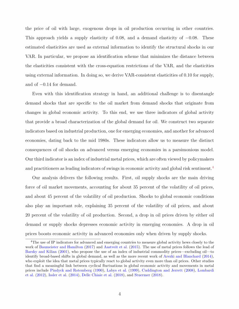
Figure 4 plots the time series of the exogenous production shortfalls. For comparison, our

time series is plotted alongside the measure of oil supply shocks constructed following Kilian

(2008). The latter is based on large drops in oil production in some OPEC countries relative

to a counterfactual based on the production of other OPEC countries which did not experience

such shocks and which were otherwise subject to the same global macroeconomic conditions

and economic incentives.16

When we compare our non-zero shocks with Kilian’s shocks in the same month—as shown

in the inset panel—the magnitudes are similar, and correlation between the two series is very

high (0.92). However, when the comparison is extended to the full set of observations in which

the two series overlay, the correlation drops to 0.68, as Kilian’s series, by construction, dis-

plays large swings also in periods without well-defined exogenous movements in oil production.

Importantly, our shocks series signals a larger exogenous oil supply drop in August 1990—

consistent with the inclusion of the United Arab Emirates along Iraq and Kuwait in the group

16We reconstruct Kilian’s monthly series following the methodology described in his paper, since Kilian’spublished oil shocks (downloaded from http://www-personal.umich.edu/~lkilian/oilshock.txt) are onlymade available at quarterly frequency. When the monthly shocks are converted to a quarterly frequency, theresulting series is virtually indistinguishable from the published series (their correlation is 0.9929).

19

of countries that were responsible for the shortfall in oil production—and includes shocks to

non-OPEC producers.

3.4 Estimation Results

We use monthly data from 1985 to 2015 on production and consumption of crude oil available

from the U.S. Department of Energy. Data on crude oil production are available for 21 countries,

while data on petroleum consumption are available for eight OECD countries. We estimate the

following instrumental variable specifications:

∆pi,τ = πi + γ∆vi,τ + εi,τ , (15)

∆qSi,τ = αS,i + ηS∆pi,τ + uSi,τ , (16)

∆qDi,τ = αD,i + ηD∆pi,τ + ΨXi,τ + uDi,τ , (17)

where πi, αS,i, and αD,i are country fixed effects, τ is the time-subscript identifying the episodes

of exogenous drops in oil production. Equation (15) is the first-stage regression, where ∆vi,τ is

the instrument, given by the percent change in global oil production directly accounted for by

the episodes listed in Table 2. Equations (16) and (17) are the IV regressions for supply and

demand. In line with the structural VAR presented in Section 2, Equation (17) controls for

contemporaneous and lagged country–specific, advanced economies, and emerging economies

log changes in IP, all denoted by the vector Xi,τ . For each country i, we construct country-

specific instruments by excluding exogenous episodes involving that country. For instance,

the instrument for the U.S. excludes the months of September 2005 and September 2008, the

two months during which hurricanes Katrina and Gustav disrupted crude oil and petroleum

products production in the U.S.

Panels (A) and (B) in Table 3 report results from the estimation of equations (16) and (17).

The OLS column presents the estimates when, trivially, ∆p = ∆p, while the last two columns

show the IV estimates using the narrow and broad instruments discussed in the previous sec-

20

tion.17

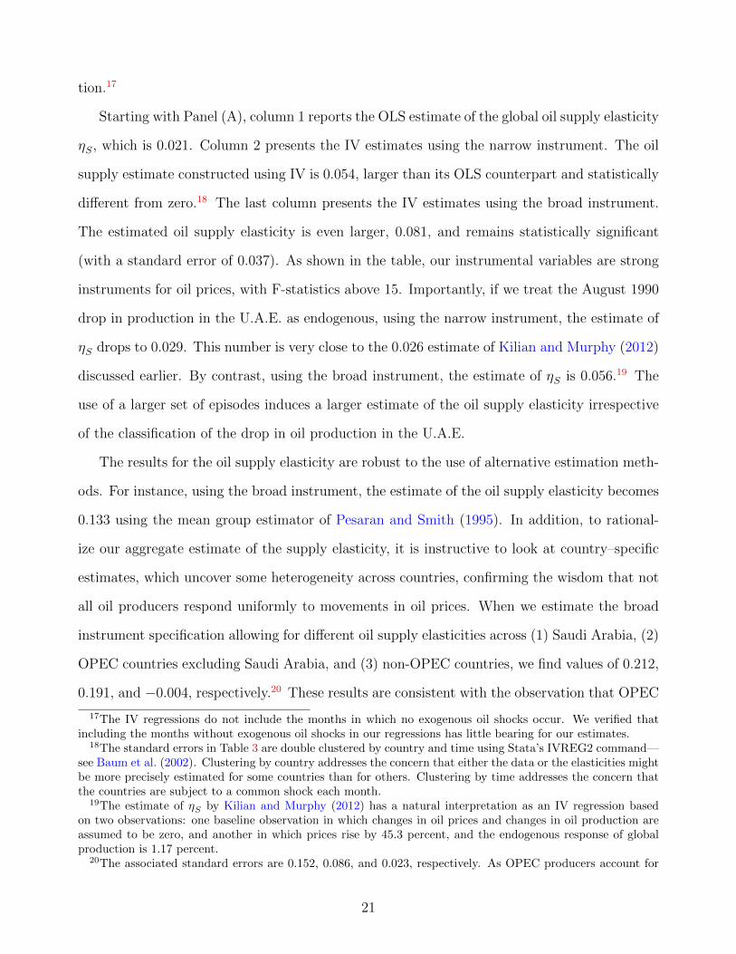
Starting with Panel (A), column 1 reports the OLS estimate of the global oil supply elasticity

ηS, which is 0.021. Column 2 presents the IV estimates using the narrow instrument. The oil

supply estimate constructed using IV is 0.054, larger than its OLS counterpart and statistically

different from zero.18 The last column presents the IV estimates using the broad instrument.

The estimated oil supply elasticity is even larger, 0.081, and remains statistically significant

(with a standard error of 0.037). As shown in the table, our instrumental variables are strong

instruments for oil prices, with F-statistics above 15. Importantly, if we treat the August 1990

drop in production in the U.A.E. as endogenous, using the narrow instrument, the estimate of

ηS drops to 0.029. This number is very close to the 0.026 estimate of Kilian and Murphy (2012)

discussed earlier. By contrast, using the broad instrument, the estimate of ηS is 0.056.19 The

use of a larger set of episodes induces a larger estimate of the oil supply elasticity irrespective

of the classification of the drop in oil production in the U.A.E.

The results for the oil supply elasticity are robust to the use of alternative estimation meth-

ods. For instance, using the broad instrument, the estimate of the oil supply elasticity becomes

0.133 using the mean group estimator of Pesaran and Smith (1995). In addition, to rational-

ize our aggregate estimate of the supply elasticity, it is instructive to look at country–specific

estimates, which uncover some heterogeneity across countries, confirming the wisdom that not

all oil producers respond uniformly to movements in oil prices. When we estimate the broad

instrument specification allowing for different oil supply elasticities across (1) Saudi Arabia, (2)

OPEC countries excluding Saudi Arabia, and (3) non-OPEC countries, we find values of 0.212,

0.191, and −0.004, respectively.20 These results are consistent with the observation that OPEC

17The IV regressions do not include the months in which no exogenous oil shocks occur. We verified thatincluding the months without exogenous oil shocks in our regressions has little bearing for our estimates.

18The standard errors in Table 3 are double clustered by country and time using Stata’s IVREG2 command—see Baum et al. (2002). Clustering by country addresses the concern that either the data or the elasticities mightbe more precisely estimated for some countries than for others. Clustering by time addresses the concern thatthe countries are subject to a common shock each month.

19The estimate of ηS by Kilian and Murphy (2012) has a natural interpretation as an IV regression basedon two observations: one baseline observation in which changes in oil prices and changes in oil production areassumed to be zero, and another in which prices rise by 45.3 percent, and the endogenous response of globalproduction is 1.17 percent.

20The associated standard errors are 0.152, 0.086, and 0.023, respectively. As OPEC producers account for

21

producers have the largest volume of spare capacity that can be used to offset disruptions in

oil supply within a short period of time.

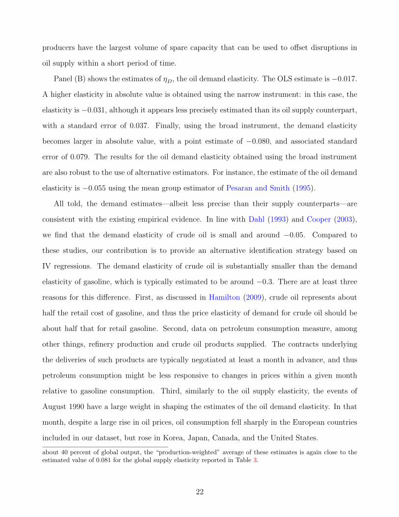
Panel (B) shows the estimates of ηD, the oil demand elasticity. The OLS estimate is −0.017.

A higher elasticity in absolute value is obtained using the narrow instrument: in this case, the

elasticity is −0.031, although it appears less precisely estimated than its oil supply counterpart,

with a standard error of 0.037. Finally, using the broad instrument, the demand elasticity

becomes larger in absolute value, with a point estimate of −0.080, and associated standard

error of 0.079. The results for the oil demand elasticity obtained using the broad instrument

are also robust to the use of alternative estimators. For instance, the estimate of the oil demand

elasticity is −0.055 using the mean group estimator of Pesaran and Smith (1995).

All told, the demand estimates—albeit less precise than their supply counterparts—are

consistent with the existing empirical evidence. In line with Dahl (1993) and Cooper (2003),

we find that the demand elasticity of crude oil is small and around −0.05. Compared to

these studies, our contribution is to provide an alternative identification strategy based on

IV regressions. The demand elasticity of crude oil is substantially smaller than the demand

elasticity of gasoline, which is typically estimated to be around −0.3. There are at least three

reasons for this difference. First, as discussed in Hamilton (2009), crude oil represents about

half the retail cost of gasoline, and thus the price elasticity of demand for crude oil should be

about half that for retail gasoline. Second, data on petroleum consumption measure, among

other things, refinery production and crude oil products supplied. The contracts underlying

the deliveries of such products are typically negotiated at least a month in advance, and thus

petroleum consumption might be less responsive to changes in prices within a given month

relative to gasoline consumption. Third, similarly to the oil supply elasticity, the events of

August 1990 have a large weight in shaping the estimates of the oil demand elasticity. In that

month, despite a large rise in oil prices, oil consumption fell sharply in the European countries

included in our dataset, but rose in Korea, Japan, Canada, and the United States.

about 40 percent of global output, the “production-weighted” average of these estimates is again close to theestimated value of 0.081 for the global supply elasticity reported in Table 3.

22

4 VAR Results

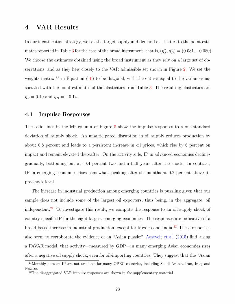
In our identification strategy, we set the target supply and demand elasticities to the point esti-

mates reported in Table 3 for the case of the broad instrument, that is, (η∗S, η∗D) = (0.081,−0.080).

We choose the estimates obtained using the broad instrument as they rely on a large set of ob-

servations, and as they hew closely to the VAR admissible set shown in Figure 2. We set the

weights matrix V in Equation (10) to be diagonal, with the entries equal to the variances as-

sociated with the point estimates of the elasticities from Table 3. The resulting elasticities are

ηS = 0.10 and ηD = −0.14.

4.1 Impulse Responses

The solid lines in the left column of Figure 5 show the impulse responses to a one-standard

deviation oil supply shock. An unanticipated disruption in oil supply reduces production by

about 0.8 percent and leads to a persistent increase in oil prices, which rise by 6 percent on

impact and remain elevated thereafter. On the activity side, IP in advanced economies declines

gradually, bottoming out at -0.4 percent two and a half years after the shock. In contrast,

IP in emerging economies rises somewhat, peaking after six months at 0.2 percent above its

pre-shock level.

The increase in industrial production among emerging countries is puzzling given that our

sample does not include some of the largest oil exporters, thus being, in the aggregate, oil

independent.21 To investigate this result, we compute the response to an oil supply shock of

country-specific IP for the eight largest emerging economies. The responses are indicative of a

broad-based increase in industrial production, except for Mexico and India.22 These responses

also seem to corroborate the evidence of an “Asian puzzle:” Aastveit et al. (2015) find, using

a FAVAR model, that activity—measured by GDP—in many emerging Asian economies rises

after a negative oil supply shock, even for oil-importing countries. They suggest that the “Asian

21Monthly data on IP are not available for many OPEC countries, including Saudi Arabia, Iran, Iraq, andNigeria.

22The disaggregated VAR impulse responses are shown in the supplementary material.

23

puzzle” can be explained by the low consumption and high investment shares in GDP, by their

high trade openness, and by the prevalence, in many countries, of price controls that attenuate

the pass-through of changes in oil prices.23

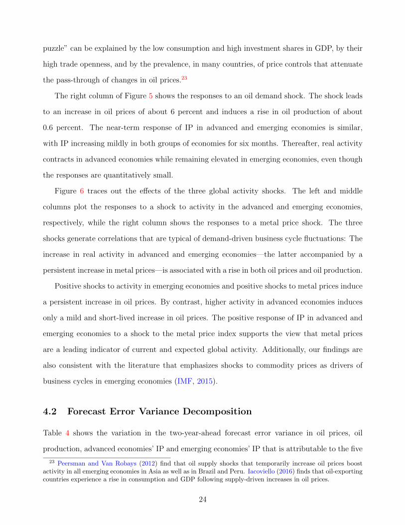
The right column of Figure 5 shows the responses to an oil demand shock. The shock leads

to an increase in oil prices of about 6 percent and induces a rise in oil production of about

0.6 percent. The near-term response of IP in advanced and emerging economies is similar,

with IP increasing mildly in both groups of economies for six months. Thereafter, real activity

contracts in advanced economies while remaining elevated in emerging economies, even though

the responses are quantitatively small.

Figure 6 traces out the effects of the three global activity shocks. The left and middle

columns plot the responses to a shock to activity in the advanced and emerging economies,

respectively, while the right column shows the responses to a metal price shock. The three

shocks generate correlations that are typical of demand-driven business cycle fluctuations: The

increase in real activity in advanced and emerging economies—the latter accompanied by a

persistent increase in metal prices—is associated with a rise in both oil prices and oil production.

Positive shocks to activity in emerging economies and positive shocks to metal prices induce

a persistent increase in oil prices. By contrast, higher activity in advanced economies induces

only a mild and short-lived increase in oil prices. The positive response of IP in advanced and

emerging economies to a shock to the metal price index supports the view that metal prices

are a leading indicator of current and expected global activity. Additionally, our findings are

also consistent with the literature that emphasizes shocks to commodity prices as drivers of

business cycles in emerging economies (IMF, 2015).

4.2 Forecast Error Variance Decomposition

Table 4 shows the variation in the two-year-ahead forecast error variance in oil prices, oil

production, advanced economies’ IP and emerging economies’ IP that is attributable to the five

23 Peersman and Van Robays (2012) find that oil supply shocks that temporarily increase oil prices boostactivity in all emerging economies in Asia as well as in Brazil and Peru. Iacoviello (2016) finds that oil-exportingcountries experience a rise in consumption and GDP following supply-driven increases in oil prices.

24

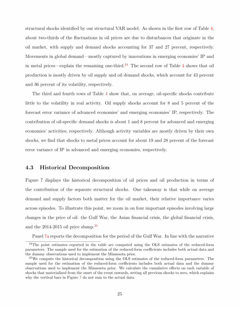
structural shocks identified by our structural VAR model. As shown in the first row of Table 4,

about two-thirds of the fluctuations in oil prices are due to disturbances that originate in the

oil market, with supply and demand shocks accounting for 37 and 27 percent, respectively.

Movements in global demand—mostly captured by innovations in emerging economies’ IP and

in metal prices—explain the remaining one-third.24 The second row of Table 4 shows that oil

production is mostly driven by oil supply and oil demand shocks, which account for 43 percent

and 36 percent of its volatility, respectively.

The third and fourth rows of Table 4 show that, on average, oil-specific shocks contribute

little to the volatility in real activity. Oil supply shocks account for 8 and 5 percent of the

forecast error variance of advanced economies’ and emerging economies’ IP, respectively. The

contribution of oil-specific demand shocks is about 1 and 8 percent for advanced and emerging

economies’ activities, respectively. Although activity variables are mostly driven by their own

shocks, we find that shocks to metal prices account for about 19 and 28 percent of the forecast

error variance of IP in advanced and emerging economies, respectively.

4.3 Historical Decomposition

Figure 7 displays the historical decomposition of oil prices and oil production in terms of

the contribution of the separate structural shocks. One takeaway is that while on average

demand and supply factors both matter for the oil market, their relative importance varies

across episodes. To illustrate this point, we zoom in on four important episodes involving large

changes in the price of oil: the Gulf War, the Asian financial crisis, the global financial crisis,

and the 2014-2015 oil price slump.25

Panel 7a reports the decomposition for the period of the Gulf War. In line with the narrative

24The point estimates reported in the table are computed using the OLS estimates of the reduced-formparameters. The sample used for the estimation of the reduced-form coefficients includes both actual data andthe dummy observations used to implement the Minnesota prior.

25We compute the historical decomposition using the OLS estimates of the reduced-form parameters. Thesample used for the estimation of the reduced-form coefficients includes both actual data and the dummyobservations used to implement the Minnesota prior. We calculate the cumulative effects on each variable ofshocks that materialized from the onset of the event onwards, setting all previous shocks to zero, which explainswhy the vertical bars in Figure 7 do not sum to the actual data.

25

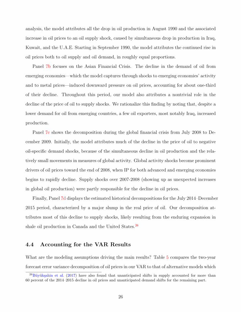
analysis, the model attributes all the drop in oil production in August 1990 and the associated

increase in oil prices to an oil supply shock, caused by simultaneous drop in production in Iraq,

Kuwait, and the U.A.E. Starting in September 1990, the model attributes the continued rise in

oil prices both to oil supply and oil demand, in roughly equal proportions.

Panel 7b focuses on the Asian Financial Crisis. The decline in the demand of oil from

emerging economies—which the model captures through shocks to emerging economies’ activity

and to metal prices—induced downward pressure on oil prices, accounting for about one-third

of their decline. Throughout this period, our model also attributes a nontrivial role in the

decline of the price of oil to supply shocks. We rationalize this finding by noting that, despite a

lower demand for oil from emerging countries, a few oil exporters, most notably Iraq, increased

production.

Panel 7c shows the decomposition during the global financial crisis from July 2008 to De-

cember 2009. Initially, the model attributes much of the decline in the price of oil to negative

oil-specific demand shocks, because of the simultaneous decline in oil production and the rela-

tively small movements in measures of global activity. Global activity shocks become prominent

drivers of oil prices toward the end of 2008, when IP for both advanced and emerging economies

begins to rapidly decline. Supply shocks over 2007-2008 (showing up as unexpected increases

in global oil production) were partly responsible for the decline in oil prices.

Finally, Panel 7d displays the estimated historical decompositions for the July 2014–December

2015 period, characterized by a major slump in the real price of oil. Our decomposition at-

tributes most of this decline to supply shocks, likely resulting from the enduring expansion in

shale oil production in Canada and the United States.26

4.4 Accounting for the VAR Results

What are the modeling assumptions driving the main results? Table 5 compares the two-year

forecast error variance decomposition of oil prices in our VAR to that of alternative models which

26Buyuksahin et al. (2017) have also found that unanticipated shifts in supply accounted for more than60 percent of the 2014–2015 decline in oil prices and unanticipated demand shifts for the remaining part.

26

differ for the choice of variables, sample period, and identification assumptions.27 The central

finding is that the short-run oil supply elasticity is the key determinant for the importance of

oil supply shocks in oil price fluctuations.

The top row summarizes our baseline VAR, estimated from 1985 through 2015, and featuring

a supply elasticity of 0.10 and a demand elasticity of −0.14. Under our baseline identification,

shocks to oil supply and shocks to global demand account for 36.5 and 37 percent of the

fluctuations in oil prices, respectively. By contrast, under an identification scheme in which

the oil supply elasticity is restricted to be zero (row 2), the volatility of oil prices that is

explained by oil supply shocks drops to 2 percent, while the contribution of global demand

shocks remains as high as in the baseline. Rows 3, 4 and 5 modify the baseline VAR with

a different set of variables, each time re-estimating supply and demand elasticities by using

the minimum distance approach described in Section 2. Rows 3 and 4 show that adding oil

inventories to our VAR, as done by Kilian and Murphy (2014) and Baumeister and Hamilton

(2017), does not materially change our results. Row 5 considers the role of the metal price

index. Dropping metal prices from our specification enhances the contribution of oil supply

shocks to fluctuations in oil prices, while reducing the contribution of global demand shocks.

Row 6 replaces our activity indicators with Kilian (2009)’s indicator of real activity based on

ocean freight rates (rea). Oil supply shocks remain important drivers of oil prices, while global

demand shocks contribute to 33.5 percent of the volatility of oil prices, somewhat less than in

our baseline VAR.

Rows 7 and 8 show that the elasticities play a crucial role in explaining the role of supply

shocks to oil price fluctuations using the variables and the sample period in Kilian (2009) (see

the supplementary material for details). The assumption of a zero short-run oil supply elasticity

results here in a VAR-consistent demand elasticity of −3.48, a very large number, and implies

that oil supply shocks play a negligible role in accounting for oil price fluctuations. By contrast,

when we minimize the distance between the elasticities derived in our panel and those that are

implied by Kilian’s VAR specification, we derive VAR-consistent elasticities of 0.18 for supply,

27The supplementary material contains details as well as a number of other robustness checks.

27

and of −0.36 for demand. These elasticities in turn imply that supply shocks account for about

one quarter of the two-year volatility in oil prices.

In sum, our findings show that the selection of the elasticities is the key reason why our

baseline VAR attributes an important role to oil supply shocks as drivers of oil prices.

5 Conclusion

Using external information from a large panel of countries, we impose restrictions on the short-

run price elasticities of oil supply and oil demand in order to identify a structural VAR model

of the global oil market. In the estimating framework, global demand for oil is jointly captured

by industrial production in advanced and emerging economies as well as by an index of metal

prices. Shocks to oil supply and shock to global demand each account for about one-third of

the fluctuations in oil prices at business cycle frequencies. An increase in oil prices driven by oil

supply shocks depresses industrial production in advanced economies, while it boosts industrial

production in emerging economies, thus helping explain the muted effects of changes in oil

prices on global economic activity.

28

References

Aastveit, K. A., H. C. Bjrnland, and L. A. Thorsrud (2015). What Drives Oil Prices? Emergingversus Developed Economies. Journal of Applied Econometrics 30 (7), 1013–1028.

Arezki, R. and O. J. Blanchard (2014). Seven Questions about the Recent Oil PriceSlump. IMFBlog, https://blogs.imf.org/2014/12/22/seven-questions-about-the-

recent-oil-price-slump/.

Barsky, R. B. and L. Kilian (2001). Do We Really Know That Oil Caused the Great Stagflation?A Monetary Alternative. In B. S. Bernanke and K. Rogoff (Eds.), NBER MacroeconomicsAnnual, Volume 16, pp. 137–183. MIT Press.

Baum, C. F., M. E. Schaffer, and S. Stillman (2002). IVREG2: Stata module for extendedinstrumental variables/2SLS and GMM estimation. Statistical Software Components, BostonCollege Department of Economics, https://ideas.repec.org/c/boc/bocode/s425401.

html.

Baumeister, C. and J. D. Hamilton (2017). Structural Interpretation of Vector Autoregres-sions with Incomplete Identification: Revisiting the Role of Oil Supply and Demand Shocks.National Bureau of Economic Research Working Paper no. 24167.

Baumeister, C. and G. Peersman (2013a). The Role of Time-Varying Price Elasticities inAccounting for Volatility Changes in the Crude Oil Market. Journal of Applied Economet-rics 28 (7), 1087–1109.

Baumeister, C. and G. Peersman (2013b). Time-Varying Effects of Oil Supply Shocks on theU.S. Economy. American Economic Journal: Macroeconomics 5 (4), 1–28.

Beidas-Strom, S. and A. Pescatori (2014). Oil Price Volatility and the Role of Speculation.Working Paper 14/218, IMF.

Blanchard, O. J. and J. Galı (2010). The Macroeconomic Effects of Oil Price Shocks: Whyare the 2000s so different from the 1970s? In J. Galı and M. Gertler (Eds.), InternationalDimensions of Monetary Policy, Chapter 7, pp. 373–421. University of Chicago Press. http://www.nber.org/chapters/c0517.

Buyuksahin, B., D. Bilgin, R. Ellwanger, K. Mo, and K. Zmitrowicz (2017). What Causedthe 2014-2015 Oil Price Drop? Evidence from Global Fuel Consumption. UnpublishedManuscript, Bank of Canada.

Coglianese, J., L. W. Davis, L. Kilian, and J. H. Stock (2017). Anticipation, Tax Avoidance,and the Price Elasticity of Gasoline Demand. Journal of Applied Econometrics 32 (1), 1–15.

Cooper, J. C. (2003). Price Elasticity of Demand for Crude Oil: Estimates for 23 Countries.OPEC Review 27 (1), 1–8.

Cuddington, J. T. and D. Jerrett (2008). Super Cycles in Real Metals Prices? IMF StaffPapers 55, 541–565.

29

Dahl, C. (1993). A Survey of Oil Demand Elasticities for Developing Countries. OPEC Re-view 17 (4), 399–420.

Dees, S., F. di Mauro, M. H. Pesaran, and L. V. Smith (2007). Exploring the InternationalLinkages of the Euro Area: A Global VAR Analysis. Journal of Applied Econometrics 22 (1),1–38.

Del Negro, M. and F. Schorfheide (2011). Bayesian Macroeconometrics. In J. Geweke, G. Koop,and H. van Dijk (Eds.), The Oxford Handbook of Bayesian Econometrics, Chapter 7, pp. 293–389. Oxford University Press.

Delle Chiaie, S., L. Ferrara, and D. Giannone (2018). Common Factors of Commodity Prices.Center for Economic Policy Research Discussion Paper no. 12767.

Gelman, M., Y. Gorodnichenko, S. Kariv, D. Koustas, M. D. Shapiro, D. Silverman, andS. Tadelis (2016). The Response of Consumer Spending to Changes in Gasoline Prices.National Bureau of Economic Research Working Paper no. 22969.

Hamilton, J. D. (2003). What Is an Oil Shock? Journal of Econometrics 113 (2), 363–398.

Hamilton, J. D. (2009). Causes and Consequences of the Oil Shock of 2007-08. BrookingsPapers on Economic Activity 40 (1 (Spring), 215–283.

Iacoviello, M. (2016). Oil Prices and Consumption across Countries and U.S. States. FederalReserve Board.

Ibrahim, Y. M. (1990, July 18). Iraq Threatens Emirates And Kuwait on Oil Glut. The NewYork Times , p. D1.

IMF (2015). Where Are Commodity Exporters Headed? Output Growth in the Aftermath ofthe Commodity Boom. In World Economic Outlook, Chapter 2, pp. 65–104. IMF.

Issler, J., C. Rodrigues, and R. Burkack (2014). Using Common Features to Understand theBehavior of Metal-Commodity Prices and Forecast Them at Different Horizons. Journal ofInternational Money and Finance 42, 310–335.

Juvenal, L. and I. Petrella (2015). Speculation in the Oil Market. Journal of Applied Econo-metrics 30 (4), 621–649.

Kilian, L. (2008). Exogenous Oil Supply Shocks: How Big Are They and How Much Do TheyMatter for the U.S. Economy? Review of Economics and Statistics 90 (2), 216–240.

Kilian, L. (2009). Not All Oil Price Shocks Are Alike: Disentangling Demand and SupplyShocks in the Crude Oil Market. American Economic Review 99 (3), 1053–69.

Kilian, L. and D. P. Murphy (2012). Why Agnostic Sign Restrictions Are Not Enough: Un-derstanding the Dynamics of Oil Market VAR Models. Journal of the European EconomicAssociation 10 (5), 1166–1188.

Kilian, L. and D. P. Murphy (2014). The Role of Inventories and Speculative Trading in theGlobal Market for Crude Oil. Journal of Applied Econometrics 29 (3), 454–478.

30

Labys, W., A. Achouch, and M. Terraza (1999). Metal Prices and the Business Cycle. ResourcesPolicy 25 (4), 229–238.

Lippi, F. and A. Nobili (2012). Oil and The Macroeconomy: A Quantitative Structural Analysis.Journal of the European Economic Association 10 (5), 1059–1083.

Lombardi, M. J., C. Osbat, and B. Schnatz (2012). Global Commodity Cycles and Llinkages:A FAVAR Approach. Empirical Economics 55, 541–565.

Mohaddes, K. and M. H. Pesaran (2016). Country-Specific Oil Supply Shocks and the GlobalEconomy: A Counterfactual Analysis. Energy Economics 59, 382–399.

Peersman, G. and I. Van Robays (2012). Cross-Country Differences in the Effects of Oil Shocks.Energy Economics 34 (5), 1532–1547.

Pesaran, M. H. and R. Smith (1995). Estimating Long-Run Relationships from Dynamic Het-erogeneous Panels. Journal of Econometrics 68 (1), 79–113.

Pindyck, R. S. and J. J. Rotemberg (1990). The Excess Co-movement of Commodity Prices.Economic Journal 100 (403), 1173–89.

Rotemberg, J. J. and M. Woodford (1996). Imperfect Competition and the Effects of EnergyPrice Increases on Economic Activity. Journal of Money, Credit and Banking 28 (4), 550–577.

Rubio-Ramırez, J. F., D. F. Waggoner, and T. Zha (2010). Structural Vector Autoregressions:Theory of Identification and Algorithms for Inference. Review of Economic Studies 77 (2),665–96.

Shapiro, M. D. and M. W. Watson (1988). Sources of Business Cycles Fluctuations. In S. Fischer(Ed.), NBER Macroeconomics Annual, Volume 3, pp. 111–148. MIT Press.

Stock, J. and M. Watson (2016). Dynamic Factor Models, Factor-Augmented Vector Autore-gressions, and Structural Vector Autoregressions in Macroeconomics. In J. B. Taylor andH. Uhlig (Eds.), Handbook of Macroeconomics, Volume 2A, Chapter 8, pp. 415–525. Elsevier.

Stuermer, M. (2018). 150 Years of Boom and Bust: What Drives Mineral Commodity Prices?Macroeconomic Dynamics 22 (3), 702–717.

31

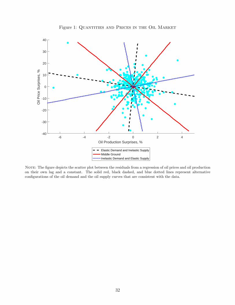
Figure 1: Quantities and Prices in the Oil Market

-6 -4 -2 0 2 4

Oil Production Surprises, %

-40

-30

-20

-10

0

10

20

30

40O

il P

rice

Sur

pris

es, %

Elastic Demand and Inelastic SupplyMiddle GroundInelastic Demand and Elastic Supply

Note: The figure depicts the scatter plot between the residuals from a regression of oil prices and oil productionon their own lag and a constant. The solid red, black dashed, and blue dotted lines represent alternativeconfigurations of the oil demand and the oil supply curves that are consistent with the data.

32

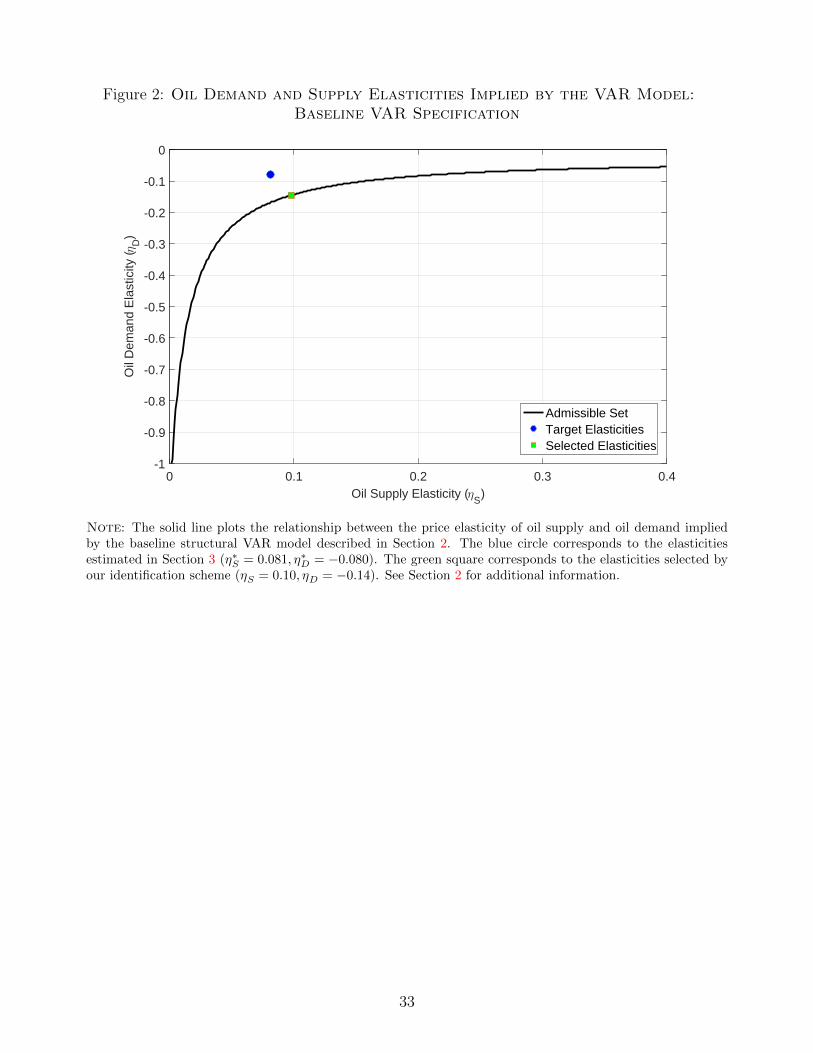
Figure 2: Oil Demand and Supply Elasticities Implied by the VAR Model:Baseline VAR Specification

0 0.1 0.2 0.3 0.4Oil Supply Elasticity (2

S)

-1

-0.9

-0.8

-0.7

-0.6

-0.5

-0.4

-0.3

-0.2

-0.1

0

Oil

Dem

and

Ela

stic

ity ( 2

D)

Admissible SetTarget ElasticitiesSelected Elasticities

Note: The solid line plots the relationship between the price elasticity of oil supply and oil demand impliedby the baseline structural VAR model described in Section 2. The blue circle corresponds to the elasticitiesestimated in Section 3 (η∗S = 0.081, η∗D = −0.080). The green square corresponds to the elasticities selected byour identification scheme (ηS = 0.10, ηD = −0.14). See Section 2 for additional information.

33

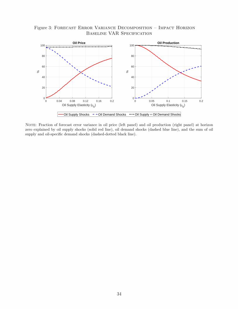
Figure 3: Forecast Error Variance Decomposition – Impact HorizonBaseline VAR Specification

0 0.04 0.08 0.12 0.16 0.2

Oil Supply Elasticity (2S

)

0

20

40

60

80

100

%

Oil Price

Oil Supply Shocks Oil Demand Shocks Oil Supply + Oil Demand Shocks

0 0.05 0.1 0.15 0.2

Oil Supply Elasticity (2S

)

0

20

40

60

80

100

%

Oil Production

Note: Fraction of forecast error variance in oil price (left panel) and oil production (right panel) at horizonzero explained by oil supply shocks (solid red line), oil demand shocks (dashed blue line), and the sum of oilsupply and oil-specific demand shocks (dashed-dotted black line).

34

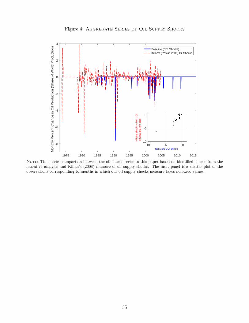
Figure 4: Aggregate Series of Oil Supply Shocks

1975 1980 1985 1990 1995 2000 2005 2010 2015

-8

-6

-4

-2

0

2

4

Mon

thly

Per

cent

Cha

nge

in O

il P

rodu

ctio

n (S

hare

of W

orld

Pro

duct

ion) Baseline (CCI Shocks)

Kilian's (Restat, 2008) Oil Shocks

-10 -5 0Non-zero CCI shocks

-10

-5

0

Kili

an's

sho

cks

whe

n C

CI

sho

cks

are

non-

zero

Note: Time-series comparison between the oil shocks series in this paper based on identified shocks from thenarrative analysis and Kilian’s (2008) measure of oil supply shocks. The inset panel is a scatter plot of theobservations corresponding to months in which our oil supply shocks measure takes non-zero values.

35

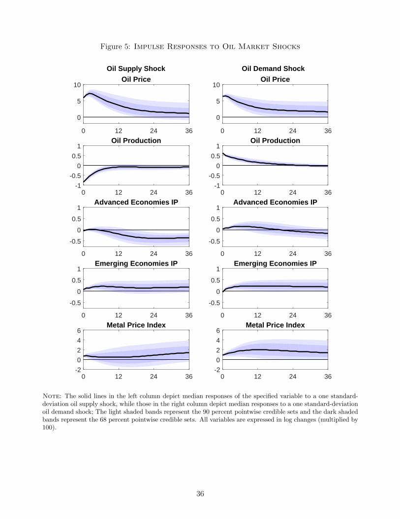
Figure 5: Impulse Responses to Oil Market Shocks

0 12 24 36

0

5

10Oil Price

0 12 24 36-1

-0.5

0

0.5

1Oil Production

0 12 24 36

-0.5

0

0.5

1Advanced Economies IP

0 12 24 36

-0.5

0

0.5

1Emerging Economies IP

0 12 24 36-2

0

2

4

6Metal Price Index

0 12 24 36

0

5

10Oil Price

0 12 24 36-1

-0.5

0

0.5

1Oil Production

0 12 24 36

-0.5

0

0.5

1Advanced Economies IP

0 12 24 36

-0.5

0

0.5

1Emerging Economies IP

0 12 24 36-2

0

2

4

6Metal Price Index

Oil Supply Shock Oil Demand Shock

Note: The solid lines in the left column depict median responses of the specified variable to a one standard-deviation oil supply shock, while those in the right column depict median responses to a one standard-deviationoil demand shock; The light shaded bands represent the 90 percent pointwise credible sets and the dark shadedbands represent the 68 percent pointwise credible sets. All variables are expressed in log changes (multiplied by100).

36

Figure 6: Impulse Responses to Global Activity Shocks

0 12 24 36

0

5

10Oil Price

0 12 24 36-0.25

0

0.25

0.5Oil Production

0 12 24 36

-0.5

0

0.5

1

Advanced Economies IP

0 12 24 36

0

0.5

1

Emerging Economies IP

0 12 24 36-4

0

4

8Metal Price Index

0 12 24 36

0

5

10Oil Price

0 12 24 36-0.25

0

0.25

0.5Oil Production

0 12 24 36

-0.5

0

0.5

1

Advanced Economies IP

0 12 24 36

0

0.5

1

Emerging Economies IP

0 12 24 36-4

0

4

8Metal Price Index

0 12 24 36

0

5

10Oil Price

0 12 24 36-0.25

0

0.25

0.5Oil Production

0 12 24 36

-0.5

0

0.5

1

Advanced Economies IP

0 12 24 36

0

0.5

1

Emerging Economies IP

0 12 24 36-4

0

4

8Metal Price Index

AE Activity Shock EE Activity Shock Metal Price ShockAE Activity Shock

Note: The solid lines in the left column depict median responses of the specified variable to a one standard-deviation shock to advanced economies’ activity, those in the middle column depict median responses to aone standard-deviation shock to emerging economies’ activity, and those in the right column depict medianresponses to a one standard-deviation metal price shock; The light shaded bands represent the 90 percentpointwise credible sets and the dark shaded bands represent the 68 percent pointwise credible sets. All variablesare expressed in log changes (multiplied by 100).

37

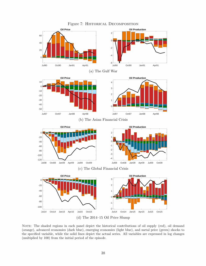
Figure 7: Historical Decomposition

Jul90 Oct90 Jan91 Apr91

0

20

40

60

Oil Price

Jul90 Oct90 Jan91 Apr91-6

-4

-2

0

2

Oil Production

(a) The Gulf War

Jul97 Oct97 Jan98 Apr98

-50

-40

-30

-20

-10

0

10

Oil Price

Jul97 Oct97 Jan98 Apr98

0

1

2

3

4

Oil Production

(b) The Asian Financial Crisis

Jul08 Oct08 Jan09 Apr09 Jul09 Oct09-120

-100

-80

-60

-40

-20

0

Oil Price

Jul08 Oct08 Jan09 Apr09 Jul09 Oct09

-4

-3

-2

-1

0

1

2

Oil Production

(c) The Global Financial Crisis

Jul14 Oct14 Jan15 Apr15 Jul15 Oct15

-100

-80

-60

-40

-20

0

Oil Price

Jul14 Oct14 Jan15 Apr15 Jul15 Oct15-2

-1

0

1

2

3

Oil Production

(d) The 2014–15 Oil Price Slump

Note: The shaded regions in each panel depict the historical contributions of oil supply (red), oil demand(orange), advanced economies (dark blue), emerging economies (light blue), and metal price (green) shocks tothe specified variable, while the solid lines depict the actual series. All variables are expressed in log changes(multiplied by 100) from the initial period of the episode.

38

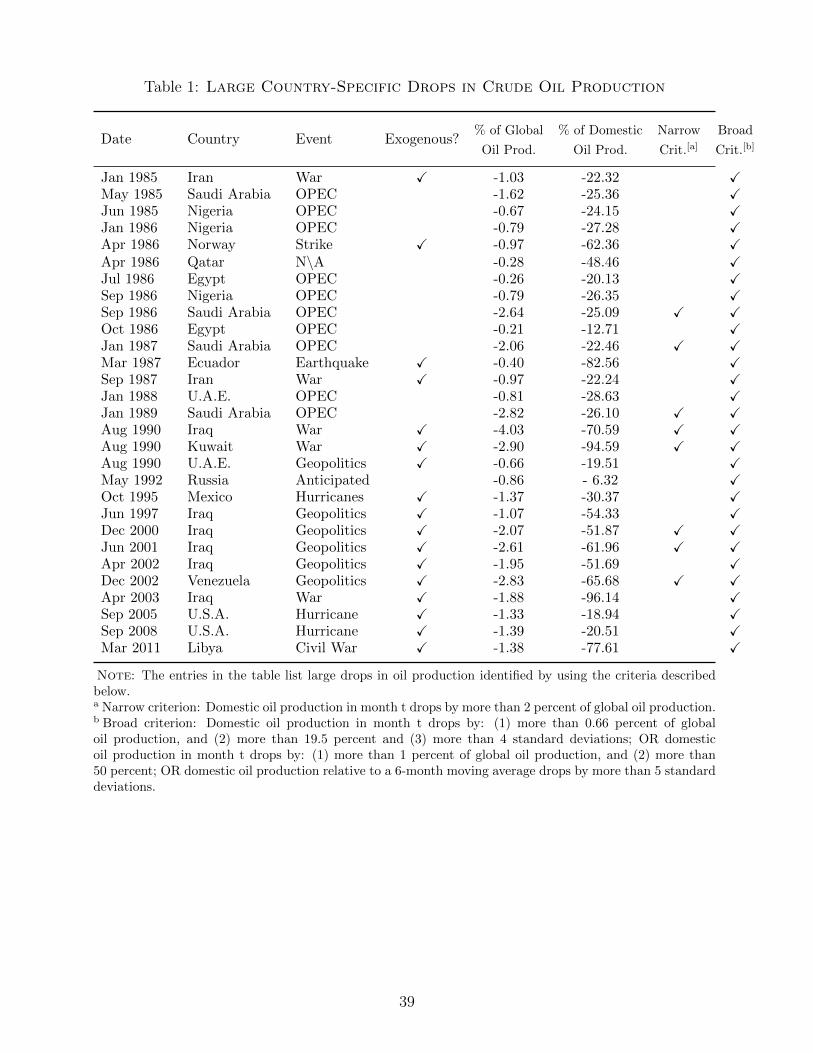
Table 1: Large Country-Specific Drops in Crude Oil Production

Date Country Event Exogenous?% of Global

Oil Prod.

% of Domestic

Oil Prod.

Narrow

Crit.[a]Broad

Crit.[b]

Jan 1985 Iran War X -1.03 -22.32 XMay 1985 Saudi Arabia OPEC -1.62 -25.36 XJun 1985 Nigeria OPEC -0.67 -24.15 XJan 1986 Nigeria OPEC -0.79 -27.28 XApr 1986 Norway Strike X -0.97 -62.36 XApr 1986 Qatar N\A -0.28 -48.46 XJul 1986 Egypt OPEC -0.26 -20.13 XSep 1986 Nigeria OPEC -0.79 -26.35 XSep 1986 Saudi Arabia OPEC -2.64 -25.09 X XOct 1986 Egypt OPEC -0.21 -12.71 XJan 1987 Saudi Arabia OPEC -2.06 -22.46 X XMar 1987 Ecuador Earthquake X -0.40 -82.56 XSep 1987 Iran War X -0.97 -22.24 XJan 1988 U.A.E. OPEC -0.81 -28.63 XJan 1989 Saudi Arabia OPEC -2.82 -26.10 X XAug 1990 Iraq War X -4.03 -70.59 X XAug 1990 Kuwait War X -2.90 -94.59 X XAug 1990 U.A.E. Geopolitics X -0.66 -19.51 XMay 1992 Russia Anticipated -0.86 - 6.32 XOct 1995 Mexico Hurricanes X -1.37 -30.37 XJun 1997 Iraq Geopolitics X -1.07 -54.33 XDec 2000 Iraq Geopolitics X -2.07 -51.87 X XJun 2001 Iraq Geopolitics X -2.61 -61.96 X XApr 2002 Iraq Geopolitics X -1.95 -51.69 XDec 2002 Venezuela Geopolitics X -2.83 -65.68 X XApr 2003 Iraq War X -1.88 -96.14 XSep 2005 U.S.A. Hurricane X -1.33 -18.94 XSep 2008 U.S.A. Hurricane X -1.39 -20.51 XMar 2011 Libya Civil War X -1.38 -77.61 X

Note: The entries in the table list large drops in oil production identified by using the criteria describedbelow.a Narrow criterion: Domestic oil production in month t drops by more than 2 percent of global oil production.b Broad criterion: Domestic oil production in month t drops by: (1) more than 0.66 percent of globaloil production, and (2) more than 19.5 percent and (3) more than 4 standard deviations; OR domesticoil production in month t drops by: (1) more than 1 percent of global oil production, and (2) more than50 percent; OR domestic oil production relative to a 6-month moving average drops by more than 5 standarddeviations.

39

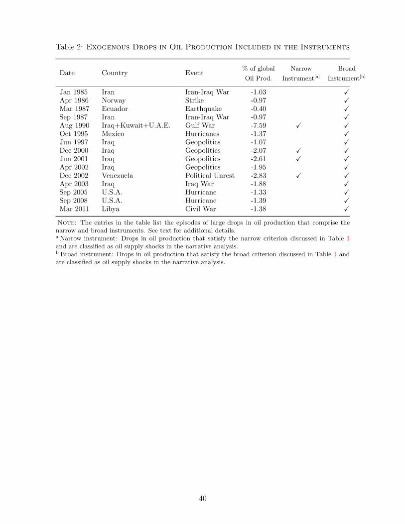
Table 2: Exogenous Drops in Oil Production Included in the Instruments

Date Country Event% of global

Oil Prod.

Narrow

Instrument[a]Broad

Instrument[b]

Jan 1985 Iran Iran-Iraq War -1.03 XApr 1986 Norway Strike -0.97 XMar 1987 Ecuador Earthquake -0.40 XSep 1987 Iran Iran-Iraq War -0.97 XAug 1990 Iraq+Kuwait+U.A.E. Gulf War -7.59 X XOct 1995 Mexico Hurricanes -1.37 XJun 1997 Iraq Geopolitics -1.07 XDec 2000 Iraq Geopolitics -2.07 X XJun 2001 Iraq Geopolitics -2.61 X XApr 2002 Iraq Geopolitics -1.95 XDec 2002 Venezuela Political Unrest -2.83 X XApr 2003 Iraq Iraq War -1.88 XSep 2005 U.S.A. Hurricane -1.33 XSep 2008 U.S.A. Hurricane -1.39 XMar 2011 Libya Civil War -1.38 X

Note: The entries in the table list the episodes of large drops in oil production that comprise thenarrow and broad instruments. See text for additional details.a Narrow instrument: Drops in oil production that satisfy the narrow criterion discussed in Table 1and are classified as oil supply shocks in the narrative analysis.b Broad instrument: Drops in oil production that satisfy the broad criterion discussed in Table 1 andare classified as oil supply shocks in the narrative analysis.

40

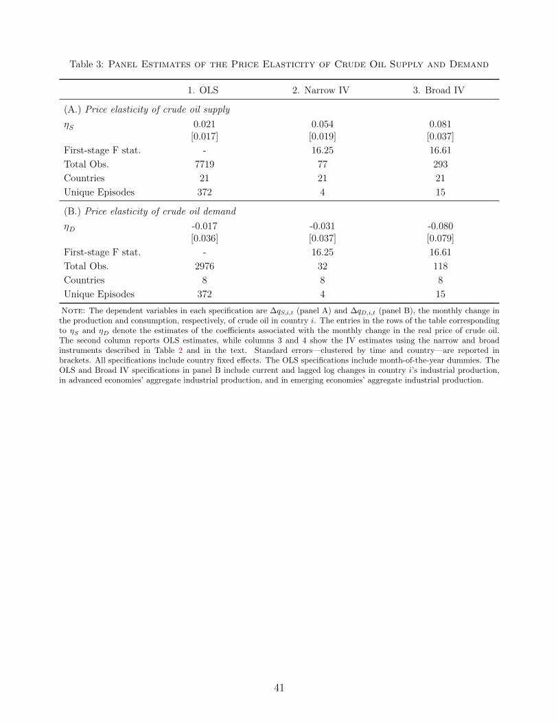
Table 3: Panel Estimates of the Price Elasticity of Crude Oil Supply and Demand

1. OLS 2. Narrow IV 3. Broad IV

(A.) Price elasticity of crude oil supply

ηS 0.021 0.054 0.081[0.017] [0.019] [0.037]

First-stage F stat. - 16.25 16.61

Total Obs. 7719 77 293

Countries 21 21 21

Unique Episodes 372 4 15

(B.) Price elasticity of crude oil demand

ηD -0.017 -0.031 -0.080[0.036] [0.037] [0.079]

First-stage F stat. - 16.25 16.61

Total Obs. 2976 32 118

Countries 8 8 8

Unique Episodes 372 4 15

Note: The dependent variables in each specification are ∆qS,i,t (panel A) and ∆qD,i,t (panel B), the monthly change inthe production and consumption, respectively, of crude oil in country i. The entries in the rows of the table correspondingto ηS and ηD denote the estimates of the coefficients associated with the monthly change in the real price of crude oil.The second column reports OLS estimates, while columns 3 and 4 show the IV estimates using the narrow and broadinstruments described in Table 2 and in the text. Standard errors—clustered by time and country—are reported inbrackets. All specifications include country fixed effects. The OLS specifications include month-of-the-year dummies. TheOLS and Broad IV specifications in panel B include current and lagged log changes in country i’s industrial production,in advanced economies’ aggregate industrial production, and in emerging economies’ aggregate industrial production.

41

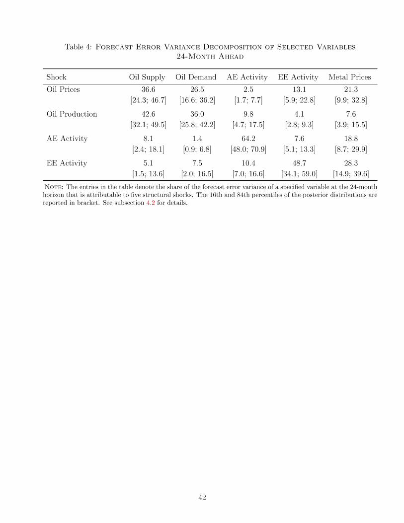
Table 4: Forecast Error Variance Decomposition of Selected Variables24-Month Ahead

Shock Oil Supply Oil Demand AE Activity EE Activity Metal Prices

Oil Prices 36.6 26.5 2.5 13.1 21.3

[24.3; 46.7] [16.6; 36.2] [1.7; 7.7] [5.9; 22.8] [9.9; 32.8]

Oil Production 42.6 36.0 9.8 4.1 7.6

[32.1; 49.5] [25.8; 42.2] [4.7; 17.5] [2.8; 9.3] [3.9; 15.5]

AE Activity 8.1 1.4 64.2 7.6 18.8

[2.4; 18.1] [0.9; 6.8] [48.0; 70.9] [5.1; 13.3] [8.7; 29.9]

EE Activity 5.1 7.5 10.4 48.7 28.3

[1.5; 13.6] [2.0; 16.5] [7.0; 16.6] [34.1; 59.0] [14.9; 39.6]

Note: The entries in the table denote the share of the forecast error variance of a specified variable at the 24-monthhorizon that is attributable to five structural shocks. The 16th and 84th percentiles of the posterior distributions arereported in bracket. See subsection 4.2 for details.

42

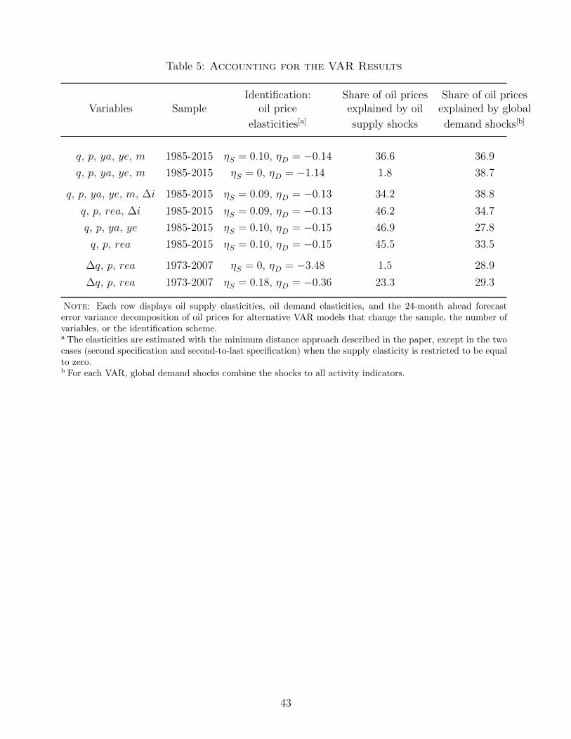
Table 5: Accounting for the VAR Results

Identification: Share of oil prices Share of oil pricesVariables Sample oil price explained by oil explained by global

elasticities[a] supply shocks demand shocks[b]

q, p, ya, ye, m 1985-2015 ηS = 0.10, ηD = −0.14 36.6 36.9

q, p, ya, ye, m 1985-2015 ηS = 0, ηD = −1.14 1.8 38.7

q, p, ya, ye, m, ∆i 1985-2015 ηS = 0.09, ηD = −0.13 34.2 38.8

q, p, rea, ∆i 1985-2015 ηS = 0.09, ηD = −0.13 46.2 34.7

q, p, ya, ye 1985-2015 ηS = 0.10, ηD = −0.15 46.9 27.8

q, p, rea 1985-2015 ηS = 0.10, ηD = −0.15 45.5 33.5

∆q, p, rea 1973-2007 ηS = 0, ηD = −3.48 1.5 28.9

∆q, p, rea 1973-2007 ηS = 0.18, ηD = −0.36 23.3 29.3

Note: Each row displays oil supply elasticities, oil demand elasticities, and the 24-month ahead forecasterror variance decomposition of oil prices for alternative VAR models that change the sample, the number ofvariables, or the identification scheme.a The elasticities are estimated with the minimum distance approach described in the paper, except in the twocases (second specification and second-to-last specification) when the supply elasticity is restricted to be equalto zero.b For each VAR, global demand shocks combine the shocks to all activity indicators.

43