May 1, 2013 The following white paper contains an examination of the price sensitivity of postal customers of three market dominant Postal Service products: First-Class Mail, Standard Mail, and Periodicals. The marketplace for traditional Postal Service products is increasingly competitive. In addition to the long term trend toward electronic media, Postal Service products face intense pressures brought about by the Great Recession. This paper explores an open question raised by these disruptive trends: Are Postal Service customers becoming more price sensitive? Though intuition may suggest that growing competition would have this effect, the answer to this question is best found by letting the data do the talking. Toward that end, this paper presents the results of an open-minded, rigorous empirical review of the demand for these postal products. Price sensitivity was analyzed with a battery of tests using both the Postal Service demand models and alternative models. The analysis was subjected to extensive peer review. We were surprised to find that, no matter how we stressed the models or which models we used, the data told the same story: Demand for postal products is not becoming more price sensitive. In fact, a case can be made that these products are becoming less price sensitive. This may be because customers most likely to leave the Postal Service for the Internet have already done so, leaving the remaining customers more loyal in the face of price increases. In the course of our analysis, we did uncover some technical problems with the Postal Service’s demand models. We recommend that the Postal Service make adjustments to its models as appropriate. These technical problems had no significant effect on our conclusions.

David C. Williams Inspector General

Analysis of Postal Price Elasticities

May 1, 2013

Report Number: RARC-WP-13-008

WHITE PAPER

U.S. Postal Service Office of Inspector General May 1, 2013 i

Analysis of Postal Price Elasticities

This paper analyzes the effect of postal price increases on revenue and volume. Opponents of price increases assert that higher prices will drive customers away, reducing revenue and exacerbating the loss of volume to electronic alternatives. Proponents of price increases cite the long history of price increases that led to revenue increases prior to the implementation of a price cap in 2007. The resolution of this dispute lies in the data. Analysis of the demand for postal products shows that price increases will increase revenues. Recent events such as the Great Recession and the growth of use of the Internet do not change this conclusion.

Economists use the concept of price elasticity to analyze the effect of price changes on revenue changes. When price increases lead to decreased revenue the demand for the product is said to be price elastic. When price increases cause revenues to increase demand is inelastic.

Price elasticity is estimated using econometric models of product demand. The Postal Service has produced its econometric demand models for more than 30 years with periodic refinements to reflect changes in the economy and postal industry. Some argue that the models provide evidence of an upward trend in price elasticity and that the price elasticity of postal customers is “in flux” due to the increase of electronic alternatives and the disruptive effects of the Great Recession.1 In order to test these propositions, this paper examines the demand for three classes of market dominant postal services: 1 United States Postal Service, Plan to Profitability: 5 Year Business Plan, February 16, 2012, http://about.usps.com/news/national-releases/2012/pr12_0217profitability.pdf, p. 4, and Five Year Business Plan, April 16, 2013, http://about.usps.com/strategic-planning/fiveyearplan-04162013-final.pdf, p. 6.

EXECUTIVE SUMMARY

Highlights

The OIG asked Christensen Associates to review the Postal Service’s demand models for First-Class Mail, Standard Mail, and Periodicals.

Christensen Associates found that these postal products are price inelastic: raising their prices will increase postal revenues. Lowering them will decrease revenues.

There was no evidence that either the long-term trend toward using electronic alternatives to mail or the Great Recession has caused postal customers to become more price sensitive.

There were some technical problems with the Postal Service models. Correcting these problems did not change the findings; the demand for these postal products is still price inelastic.

RARC-WP-13-008 Analysis of Postal Price Elasticities

U.S. Postal Service Office of Inspector General May 1, 2013 ii

First-Class Mail®, Standard Mail®, and Periodicals. These classes account for the majority of mail volume, mail revenue, and contribution to institutional costs.

The Office of Inspector General retained Lauritis R. Christensen Associates, an independent economic consulting firm, to conduct the analysis. Christensen Associates is well-known for its expertise in econometrics, productivity measurement, and regulatory industry policy analysis. The analysis is included as a technical appendix.

Christensen Associates reviewed the demand models that the Postal Service filed with the Postal Regulatory Commission in 2011 and 2012. The Postal Service uses these models in financial forecasting, pricing, marketing, and planning processes. Christensen Associates also reviewed other econometric formulations of the demand for postal services. This econometric evaluation of Postal Service price elasticities uses both the Postal Service’s models as well as an alternative set of models.

Results of Analysis The demand for the postal products studied is price inelastic. Price increases will

increase revenues. Decreases in postal prices, either through price cuts or widespread use of discounting, will reduce Postal Service revenues.

A case can be made that the demand for postal products (with the possible exception of Standard Enhanced Carrier Route (ECR) mail) has actually become more price inelastic over time. Moreover, even the most price sensitive product examined in this report, Standard Mail ECR, is price inelastic.

The Great Recession and the availability of electronic alternatives clearly decreased the demand for the postal services examined in this report, as evidenced by a drastic decline in volume over the past 7 years. However, neither the recession nor any other event since 2008 caused postal price elasticities to increase in any significant way. Postal price elasticities are not in flux. The demand for postal products remains price inelastic.

Price elasticities generally are higher when competitive alternatives are more readily available. Since electronic alternatives to mail have become increasingly widespread in recent years, one might think that price elasticity estimates that use data from an earlier, less competitive era would understate the price elasticities of mailers today. Christensen Associates found, however, that including historical data (from the 1990s, for example) in the econometric demand analysis does not materially affect the estimates of price elasticities.

Christensen Associates found technical shortcomings in the Postal Service models. Because of this, Christensen Associates ran its analysis with both the Postal Service’s models and its preferred alternatives, error correction models. Correcting these technical problems resulted in only small changes to the price elasticity estimates and had no bearing on the major results described above.

RARC-WP-13-008 Analysis of Postal Price Elasticities

U.S. Postal Service Office of Inspector General May 1, 2013 iii

Table of Contents

Introduction ..................................................................................................................... 1

What is a Demand Model? .............................................................................................. 2

Estimates of Price Elasticities over Time ......................................................................... 4

Econometric Analysis and Results .................................................................................. 5

Business Implications ...................................................................................................... 7

Appendix

Is Demand for Market Dominant Products of the U.S. Postal Service Becoming More Own Price Elastic? ................................................................................ 8

RARC-WP-13-008 Analysis of Postal Price Elasticities

U.S. Postal Service Office of Inspector General May 1, 2013 1

Analysis of Postal Price Elasticities

Introduction The adoption of Internet-based communications and the most severe economic downturn in eight decades have combined to reduce dramatically the demand for traditional postal services. Mail volume in the United States in 2012 was 160 billion pieces, 25 percent less than its peak of 213 billion pieces in 2006. The 2012 volume level is roughly the same as in the late 1980s despite a population increase of 80 million and an increase in delivery points of 37 million.2 To make matters even worse, the vast majority of the decline in volume came from the U.S. Postal Service’s most profitable products: First-Class Mail and Standard Mail.3

There have been many disruptive events for postal customers during the last 7 years. The Internet has caused a revolution in communications away from hard copy to digital. A severe economic contraction has crippled economic growth and reduced consumer demand. Postal prices have increased. Economists use econometric methods to provide a rigorous analytical framework to separate out these kinds of effects. These econometric tools are designed to provide an objective basis for understanding what happened in the past and what is likely to happen to mail volume when these factors change in the future. This paper relies on these accepted analytical tools.

Economists measure the degree to which consumers respond to price changes and alter their demand for products or services with the concept of elasticity. The measure of price elasticity is critical to making business and public policy decisions. A product is considered to be price inelastic if a 1-percent increase in price brings about a less than 1-percent decrease in volume. If a product is price inelastic, a price increase will increase gross revenue. If we can confidently conclude that the demand for a product is inelastic with respect to price, then price increases can be a powerful financial tool. When a product is price inelastic, cutting prices or discounting will be counterproductive, resulting in decreased revenue and profitability.

One way to offset the adverse financial effects of a volume decline is to raise prices. Prior to the passage of the Postal Accountability and Enhancement Act (PAEA) in 2006, the Postal Service regularly raised prices to improve its finances. Price increases were pursued because mailer demand was regarded as price inelastic. Since the passage of the PAEA, price increases have been capped at the rate of inflation except for exigent circumstances. The Postal Service has been reluctant to pursue an exigent price increase. This reluctance is based at least partially on the assumption that the Internet

2 For population data, see U.S. Census data as posted at http://www.multpl.com/united-states-population/table. For delivery points, see U.S. Postal Service figures as posed at http://about.usps.com/who-we-are/postal-history/delivery-points-since-1905.pdf. 3 Domestic First-Class Mail volume peaked at nearly 104 billion pieces in 2001. Today, there are only 69 billion pieces. Standard Mail volume peaked at nearly 104 billion pieces in 2007 and now stands at about 80 billion pieces.

RARC-WP-13-008 Analysis of Postal Price Elasticities

U.S. Postal Service Office of Inspector General May 1, 2013 2

has increased competition, thereby making mailers more sensitive to price increases. Ultimately, the question of mailer response to price increases is an empirical one.

The Postal Service maintains a set of econometric demand models that estimate, among other things, mailers’ price elasticity of demand. This paper examines these models for three market dominant classes of mail: First-Class Mail, Standard Mail, and Periodicals.4 Our examination focuses on several interrelated questions. Has the demand for these postal services experienced a structural change? In the presence of electronic alternatives and profound changes in the economy, are postal customers more price sensitive now than was previously thought? Are the Postal Service’s econometric demand models properly estimated and how, if at all, can they be improved? The U.S. Postal Service Office of Inspector General contracted with Lauritis R. Christensen Associates (Christensen Associates), an independent consulting firm with extensive postal and econometric expertise, to examine these questions. Their technical report is attached as an appendix.

What is a Demand Model? Consumers of goods and services purchase products in such a way as to maximize their satisfaction (called utility by economists) subject to a budget constraint (usually income). Businesses purchase resources to maximize profits. For most goods, this means that as prices increase, the quantity demanded decreases. This relationship gives rise to the familiar downward-sloping demand curve. There are many other factors that are important in determining the demand for goods and services. These factors include prices of substitutes and complements, consumer income, population-related factors, and changes in consumer taste and technology. These factors generally cause a demand curve to shift up or down or change shape depending on the direction of their influence on consumers.5

The actual behavioral processes that underlie the demand for a good or service are unobservable, but economists can use econometric tools to model and estimate them. These tools quantify the causal influence of each demand factor on the level of product demand. In general, when one estimates the demand for postal services, one applies some basic economic concepts of demand to specify mathematical models for estimation purposes. For postal services, these econometric models include the following demand factors:

The real price of the postal product. This is the price of the postal product itself adjusted for inflation.6 It is also called the own price.

4 According to the Postal Service’s 2012 Cost and Revenue Analysis Report, the products analyzed in this study constitute 97 percent of mail volume, 74 percent of revenue, and 81 percent of contribution to institutional costs. 5 See Figure 3 in the Christensen Associates report in the appendix for an illustration. 6 Prices are adjusted for inflation to account for the erosion of the value of the dollar over time. In this way, prior years can be compared to recent years on an even footing.

RARC-WP-13-008 Analysis of Postal Price Elasticities

U.S. Postal Service Office of Inspector General May 1, 2013 3

The real price of substitutes for the postal product. A substitute can be another postal product or a product offered by a competitor. Prices of substitutes are referred to as cross prices.

The real price of complements. A complement would be a good that is used hand-in-glove with postal products. Paper and printing are examples of complements of postal products. The prices of complements are also referred to as cross prices.

The real level of economic activity. The greater the level of economic activity, the greater is the demand for postal products. Real retail sales and employment are examples.

Population. Higher population means more consumers and more demand for postal products.

Changes in consumer tastes and technology. Examples include the availability of electronic alternatives to mail, such as electronic bill payment.

Seasonal effects, such as the pre-Christmas increase in catalogue mailing.

Other factors and events such as elections, the decennial census, changes to the definition of a product, the anthrax attacks, and the like.

The specific drivers of the demand for each postal product, of course, differ. Nevertheless, demand for all postal products follows these same basic economic principles.

Most postal demand factors have a known direction of influence on demand, but the effects of technology and taste can be either positive or negative, often in subtle and surprising ways. In the 1970s, the expansion of the use of computers was famously predicted to bring about the paperless office.7 Using similar reasoning, a 1977 commission on the future of the Postal Service predicted the decline of mail volume growth in the 1980s.8 Rather than become paperless, we experienced a boom in the use of paper in the office (and beyond). People were reluctant to give up paper, a medium that had been ubiquitous for hundreds of years. Laser printing made printing easy and convenient. Inexpensive computer technology made it easier to develop mailing lists that facilitated direct mail advertising campaigns. Instead of experiencing a

7 For the original article, see “The Office of the Future,” Business Week, June 30, 1975, http://www.businessweek.com/stories/1975-06-30/the-office-of-the-futurebusinessweek-business-news-stock-market-and-financial-advice. For an interesting discussion of why it turned out to be such a bad prediction, see Gordon Kelly, “The Paperless Office: Why It Never Happened,” Itproportal.com, March 9, 2012, http://www.itproportal.com/2012/03/09/paperless-office-why-it-never-happened. 8 Commission on Postal Service, Report on the Commission on Postal Service (Washington, DC: Government Printing Office, April 1977), p. 30.

RARC-WP-13-008 Analysis of Postal Price Elasticities

U.S. Postal Service Office of Inspector General May 1, 2013 4

decline in mail volume in the 1980s, the Postal Service saw a sharp increase aided by the very computer technology that was supposed to cause the decline.9

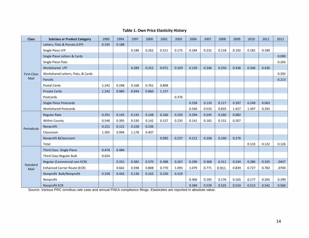
Estimates of Price Elasticities over Time The Postal Service has a long history of using econometric tools to estimate the demand for its products. Estimates of price elasticity for market dominant products are publically available. Table 1 in the Christensen Associates appendix lists these estimates over the last two-and-a-half decades.

An elasticity estimate less than 1.0 indicates that demand for a product is price inelastic. Of the 133 values listed, only nine (less than seven percent) are above 1.0, indicating elastic demand. Moreover, all of the price elasticities from 2011 or 2012, the most recent years listed, are less than 1.0. Another interesting fact is that year-to-year fluctuations in the Postal Service’s price elasticities are not a recent phenomenon. The estimated price elasticity for Within County Periodicals, for example, follows a saw tooth pattern, declining in one year and increasing the next. Finally, there does not seem to be any discernible trend toward higher elasticity values in recent years.

Somewhat ironically, the Postal Service’s econometrician takes issue with using this table to find evidence of trends in price elasticities. Each price elasticity listed comes from a demand model that estimates a single price elasticity applicable over the entire period included in the analysis, often more than 20 years in length. In the view of the Postal Service’s econometrician, the best estimates of today’s price elasticities are the most recent ones, because they include all currently available information.10

Additionally, changes in the elasticity from one set of models to the next generally reflect changes to the specification of the model, not changes in underlying mailer behavior. One such model change could be the use of a different economic activity measure, using retail sales instead of disposable income, for example. Using a different economic variable might be done because it allows the demand model to better fit historical data. Another reason for changing a demand driver is that the old driver may no longer be useful for forecasting purposes. Broadband adoption, for example, is an obvious choice to represent the expansion of the Internet, but broadband adoption stalled for several years at about two-thirds of American households. Basing a mail volume forecast on this data series would be nonsensical since we expect the Internet to have an increasing effect on mail demand for many years to come. Using different demand drivers in the models can change the estimates of all the elasticities, including its own price elasticity, even when the underlying mailer behavior has not changed.

With a few exceptions, Table 1 in the appendix shows that the Postal Service has consistently found that the demand for market dominant products is price inelastic,

9 Of course, to some extent, these pessimistic prognosticators were right; they just missed on the timing of these events by 20 years or so. 10 Thomas. E, Thress, “Response of Postal Service Witness Thress to Interrogatories of ABA-NAPM” in Postal Regulatory Commission, Transcript, Volume 6, Docket No. R2006-1, August 9, 2006, http://www.prc.gov/Docs/52/52241/Vol-6-R2006-1.pdf, pp. 1201-1203.

RARC-WP-13-008 Analysis of Postal Price Elasticities

U.S. Postal Service Office of Inspector General May 1, 2013 5

sometimes extremely so.11 Traditional economic theory states that one determinant of price elasticity is intensity of competition: The more competition, the higher the price elasticity. Low postal price elasticities in recent years seem at odds with the emerging intense competition from the Internet and other electronic alternatives to mail. There is an alternative school of thought, however, that supports low or even declining price elasticities. Suppose the market consists of two classes of customers: the Traditionals and the Digitals. The Traditionals stick with an old technology through thick and thin because it meets their business and personal needs. The Digitals look to new alternatives and once they switch to that alternative they do not switch back. If Traditionals are less price elastic than Digitals, the movement of the Digitals to the new alternatives would cause the price elasticity for the users of the old technology to decline over time.12 In the case of the Postal Service, there are some Traditionals who prefer to use hard-copy mail as opposed to electronic alternatives, and Digitals who have already switched to e-mail, electronic bill payment, and other forms of digital communication. The postal customer base may now be made of Traditionals who are unlikely to abandon their mail usage even in the face of a price increase.

The Great Recession could also affect price elasticities. It could be the case that the disruptive effects of the Great Recession have fundamentally changed the demand for postal products. For example, recession-induced pressure to reduce costs may intensify mailers’ desire to move customers to electronic bill payment, and electronic bill and statement presentment.

A formal analysis of these phenomena would answer the technical question: Has a structural change in demand caused price elasticities to increase significantly in recent times? This sort of change would reveal itself in the data and can be tested easily. The Christensen Associates analysis performs these tests.

Econometric Analysis and Results The econometric analysis followed two tracks. The first track used the Postal Service’s most recent demand models and subjected them to four separate analytical reviews. Because technical problems were discovered in the Postal Service’s models, an alternative set of models was developed. These alternative models were subjected to the same four analytical reviews.

11 The closer to zero, the more price inelastic a product is. 12 For a discussion of this phenomenon in the pharmaceutical industry, see U.S. Postal Service, Rebuttal Testimony of Thomas E. Thress, Transcript Volume 38, Docket R2006-1, pp.13023-24. Thress’s discussion, in turn, cites F.M. Scherer, Industrial Structure, Strategy and Public Policy (New York: Harper Collins, College Publishers, 1996), p. 377 and Richard G. Frank and David S. Salkever, “Pricing, Patent Loss, and the Market for Pharmaceuticals,” Southern Economic Journal, October 1992, pp. 165-79, http://www.people.vcu.edu/~lrazzolini/GR1993.pdf. A recent study that applies a remarkably similar approach to postal markets is Frederique Feve, Jean-Pierre Florens, Frank Rodriquez, Soterios Soteri, and Leticia Veruete-McKay, “Evaluating Demand for Letter Price Elasticities and Technology Impacts in an Evolving Communications Market is Higher than Econometricians Think?” 2012. http://idei.fr/doc/conf/pos/papers_2012/soteri.pdf (used with permission of the authors). This study does find an upward trend in price elasticity, but that the price elasticity remains “near the magnitude” of Lpeople, who we are calling Traditionals.

RARC-WP-13-008 Analysis of Postal Price Elasticities

U.S. Postal Service Office of Inspector General May 1, 2013 6

The first review estimated the demand models using a shortened version of the dataset, starting with the oldest data. The models were re-estimated adding the next most recent data point. For example, the first iteration would use the first 60 data points. The second would use 61 data points, the first 60 plus the next most recent. This exercise was repeated until all data points were included.13 The price elasticity estimate from each iteration was graphed over time. The resulting graphs shows whether the price elasticity estimates have trended up or down over time.

The second review essentially repeated the first analysis in reverse, starting with the most recent data, adding older data points one at a time.14 In this case, for example, the most recent 60 observations are used for the first estimation. The next estimation uses the most recent 61 observations, and so on. As before, the price elasticity from each iteration was graphed indicating whether the elasticities have exhibited a trend over time.

The third review sequentially estimated the demand equation over a subset of the available data, holding the size of the data subset constant. The first estimate was conducted with the oldest data. The equations were re-estimated by moving the dataset forward in time, one quarter at a time until only the most recent data were used.15 In this case, the first estimation would use the oldest 60 data points. The next estimation drops the oldest observation and adds the next most recent one, such that 60 data points are used in each iteration. The estimated price elasticity from each iteration was graphed over time. This analysis also depicts evidence of trends over time.

The fourth review involved a series of so-called dummy variable tests. These tests include a binary or dummy variable that allows the price elasticity to shift either up or down with recent events, like the Great Recession. If the estimated price elasticity increased or decreased, the dummy variable analysis measured the magnitude of the change and its statistical significance.

Both research tracks reached the following conclusions:

The demand for First-Class Mail, Standard Mail, and Periodicals is price inelastic, and Christensen Associates’ estimates are generally in the same range estimated by the Postal Service’s 2012 models. A case can be made for the proposition that Standard Enhanced Carrier Route (ECR) Mail has a price elasticity of one.16

With the possible exception of Standard ECR, Christensen Associates found no evidence that the demand for the market dominant products in this study has become more price elastic over time. In fact, one could reasonably conclude that some products have become less price elastic in recent years.

13 In the Christensen Associates report, this is called the recursive coefficient analysis. 14 The Christensen Associates report refers to this as the reverse recursive coefficient analysis. 15 This is called the rolling coefficient analysis in the Christensen Associates report. 16 A price elasticity equal to one, also called a unitary price elasticity, means that raising ECR’s price would leave gross revenue unchanged.

RARC-WP-13-008 Analysis of Postal Price Elasticities

U.S. Postal Service Office of Inspector General May 1, 2013 7

The Great Recession (or other recent events) does not seem to have had any discernible effect on price elasticities.

Use of historic data from a time with fewer electronic alternatives in the Postal Service’s demand analyses does not lead to underestimates of price elasticities.

As mentioned above, Christensen Associates found evidence of a technical problem often evident in time series analyses, in the Postal Service’s models. Christensen Associates used an alternative set of econometric models to remedy this problem. We recommend that the Postal Service review its regression diagnostics and consider using alternative modeling methods where appropriate. The use of alternative models did not change any of the above findings, but it did produce more defensible elasticity estimates and better measures of the variance of the estimates.

Business Implications One of the primary purposes of econometric demand models is to determine what factors cause (or do not cause) changes in mail volume. These models show that recent volume declines are the result of the effects of the Great Recession and the long-term trend away from printed communications. Price increases are not the cause of the Postal Service’s volume losses. Mailers are not more sensitive to price increases than in the past.

Based on the econometric evidence, raising the price level for First-Class Mail, Standard Mail, and Periodicals above the rate of inflation will increase the gross revenues of the Postal Service. However, it is important to note that each price elasticity estimate applies to an aggregate classification of mail. It may be the case that market segments within an aggregate classification examined in this report are price elastic. However, this implies that the remaining market segments within that classification are more inelastic than the overall econometric estimates.

Widespread discounting among these market dominant products that lowers price levels will reduce revenue. Such indiscriminant use of discounting, therefore, is a counterproductive pricing strategy. Mailers are unlikely to increase volume sufficiently to offset the reductions in price.

RARC-WP-13-008 Analysis of Postal Price Elasticities

U.S. Postal Service Office of Inspector General May 1, 2013 8

Appendix

Laurits R. Christensen Associates, Inc. 800 University Bay Drive, Suite 400 Madison, WI 53705-2299 Voice 608.231.2266 Fax 608.231.2108

Is Demand for Market Dominant Products of the U.S. Postal Service Becoming More Own Price Elastic? A. Thomas Bozzo Kristen L. Capogrossi B. Kelly Eakin Mithuna Srinivasan May 1, 2013

1

Table of Contents

I. INTRODUCTION AND EXECUTIVE SUMMARY ...................................................................................................... 4

I.B. SCOPE OF ANALYSIS .................................................................................................................................................. 6 II. PRICE ELASTICITY AND THE STRUCTURE OF POSTAL DEMANDS ......................................................................... 7

II.A. PRICE ELASTICITY .................................................................................................................................................... 7 II.B. HOUSEHOLD AND BUSINESS DEMAND FOR POSTAL SERVICES ........................................................................................... 9 II.C. DETERMINANTS OF THE PRICE ELASTICITY OF DEMAND ................................................................................................. 10 II.D. THE DISTINCTION BETWEEN A CHANGE IN DEMAND AND A CHANGE IN THE ELASTICITY OF DEMAND ..................................... 10

III. ECONOMETRIC ESTIMATION METHODS FOR POSTAL SERVICE DEMANDS ...................................................... 12 III.A. POSTAL SERVICE BASELINE MODELS ........................................................................................................................ 12 III.B. NONSTATIONARITY AND ERROR CORRECTION MODELS ................................................................................................ 15 III.C. MODIFIED USPS BASELINE DEMAND MODELS .......................................................................................................... 19 III.D. ERROR CORRECTION MODELS ................................................................................................................................ 22

IV. TESTING STABILITY OF OWN PRICE ELASTICIITES ............................................................................................ 23 IV.A. ROLLING AND RECURSIVE COEFFICIENT ANALYSIS ....................................................................................................... 23 IV.B. RESULTS OF ROLLING AND RECURSIVE PARAMETER ANALYSIS ....................................................................................... 25 IV.C. DUMMY VARIABLE INTERACTION MODELS ................................................................................................................ 39

V. CONCLUSIONS ................................................................................................................................................. 42 APPENDIX A: PRICE ELASTICITY AND THE ECONOMIC STRUCTURE OF POSTAL DEMANDS ................................... 43

A.1. PRICING AND THE IMPORTANCE OF THE ELASTICITY OF DEMAND .................................................................................... 43 A.2. DETERMINANTS OF THE PRICE ELASTICITIES OF HOUSEHOLD DEMAND ............................................................................. 44 A.3. DETERMINANTS OF THE PRICE ELASTICITIES OF BUSINESS DEMAND ................................................................................. 46 A.4. ALL OTHER THINGS AREN’T THE SAME: HOW THE DEMAND AND THE ELASTICITY OF DEMAND FOR POSTAL SERVICES MIGHT—OR MIGHT NOT—BE CHANGING ......................................................................................................................................... 49 A.5. CONCLUSION ....................................................................................................................................................... 50

APPENDIX B: SUMMARY OF CRRI CONFERENCE PAPERS REVIEWED .................................................................... 51 B.1. TIME SERIES MODELS ............................................................................................................................................ 51 DISCRETE CHOICE MODEL OF CIGNO, PEARSALL, AND PATEL ................................................................................................ 52

2

List of Tables Table 1. Own Price Elasticity History ............................................................................................ 14 Table 2. Results of Stationarity and Cointegtration Tests for Postal Service Demand Variables . 18 Table 3. Comparison of Long-Run Own Price Elasticities from USPS Demand Models and LRCA Modified Baseline Models, Full Sample Periods Ending Q4 FY2011 and Q4 FY2012 ................... 21 Table 4. Long-run Own Price Elasticities from Error Correction Models, Full Sample Periods Ending Q4 FY2011 and Q4 FY2012 ................................................................................................ 23 Table 5. Results from Dummy Variable Interaction Models ........................................................ 40

3

List of Figures Figure 1: Relative Elasticity ............................................................................................................. 8 Figure 2: Perfectly Elastic Demand and Perfectly Inelastic Demand .............................................. 9 Figure 3: Demand Decreases and Impacts on Elasticity of Demand ............................................ 11 Figure 4a. Rolling and Recursive Analysis for Standard Regular, Modified Baseline ................... 26 Figure 4b. Rolling and Recursive Analysis for Standard Mail Regular, ECM Version 1 ................. 26 Figure 5a. Rolling and Recursive Analysis for Standard ECR, Modified Baseline ......................... 27 Figure 5b. Rolling and Recursive Analysis for Standard ECR, ECM Version 1 ............................... 28 Figure 6a. Rolling and Recursive Analysis for Standard Nonprofit, Modified Baseline ................ 29 Figure 6b. Rolling and Recursive Analysis for Standard Nonprofit, ECM Version 1 ..................... 29 Figure 7a. Rolling and Recursive Analysis for Standard Nonprofit ECR, Modified Baseline ......... 30 Figure 7b. Rolling and Recursive Analysis for Standard Nonprofit ECR, ECM Version 1 .............. 31 Figure 8a. Rolling and Recursive Analysis for Periodicals, Modified Baseline .............................. 32 Figure 8b. Rolling and Recursive Analysis for Periodicals, ECM Version 1 ................................... 32 Figure 9a. Rolling and Recursive Analysis for Single Piece First-Class Mail, Modified Baseline ... 33 Figure 9b. Rolling and Recursive Analysis for Single Piece First-Class Mail, ECM Version 1 ........ 34 Figure 10a. Rolling and Recursive Analysis for Workshared First-Class, Modified Baseline ........ 35 Figure 10b. Rolling and Recursive Analysis for Workshared First-Class, ECM Version 1 ............. 35 Figure 11a. Rolling and Recursive Analysis for Single Piece First-Class Cards, Modified Baseline ......................................................................................................................................... 36 Figure 11b. Rolling and Recursive Analysis for Single Piece First-Class Cards, ECM Version 1 .... 37 Figure 12a. Rolling and Recursive Analysis for Workshared First-Class Cards, Modified Baseline ......................................................................................................................................... 38 Figure 12b. Rolling and Recursive Analysis for Workshared First-Class Cards, ECM Version 1 ... 38

4

I. INTRODUCTION AND EXECUTIVE SUMMARY

The price elasticity of demand is a concept that measures customers’ response to price changes for a product. From a seller’s point of view, the price elasticity of demand is important information for determining pricing strategies. The own price elasticity of demand specifically measures the degree of response of a product’s volume (demand) to changes in the product price. Since demand curves are generally downward sloping in the product price, own price elasticities are almost always assumed to be negative, so price increases reduce quantity demanded, other things equal. For example, if a product’s own price demand elasticity is -0.2, then a one percent increase in the (real) price of the product would result in a 0.2 percent decline in volume. Own price elasticities less than unity in absolute value are termed “inelastic;” if the volume response is larger in percentage terms than the price change, then the elasticity is greater than 1 in absolute value and demand is “elastic.”1 Among other considerations, raising the price of an own price inelastic product will increase a firm’s revenues, net of expected volume losses. The Postal Service has estimated demand models for many years, which have found inelastic demands for most market dominant postal products. However, in the wake of large and persistent volume declines for key market dominant products such as First-Class Mail letters and Standard Mail flats, the Postal Service and other parties have claimed that postal demand may have become more own price elastic over time, potentially due to factors such as increased competition from electronic substitutes or increased price sensitivity of mailers seeking cost savings as a result of the Great Recession. These claims bear on a number of important pricing issues, including the utility of exigent rate increases, and the effects of rate rebalancing in which certain products within mail classes may face systematic increases in real price to meet regulatory cost coverage requirements. While the Postal Service’s demand models incorporate features to account Internet diversion and cyclical economic effects, they do not directly provide for changes in own price elasticities of demand. The history of own price elasticities from the demand models provides some indication of the sensitivity of the results to the inclusion of data from more recent years. If adding data to the end of a demand model sample caused a large increase in the measured elasticity, it would be appropriate to conclude that demands were becoming more elastic over time. However, it is possible that the long sample periods and other model assumptions could attenuate changes in the elasticities, so the lack of longer-range trends in the elasticity histories is not dispositive of the question of whether own price elasticities are increasing or otherwise “in flux.” Our analysis addresses a primary question of interest, “Can the Postal Service’s demand models be used to test the proposition that the price elasticity of demand has changed as a result of the Internet or other recent events?” We review the theory of demand, including consumer demands for goods and services and firms’ demands for factors of production, to assess

1 In the discussion below, we mean “larger” own price elasticities to refer to elasticities that are larger in absolute value—that is, more own price elastic demands.

5

whether recent changes to postal and communications markets necessarily imply increasing own price elasticities for the Postal Service’s market dominant products. Section II summarizes our review of demand issues, which is presented in Appendix A. We also reviewed the Postal Service’s econometric models of market dominant product demands, filed with the Postal Regulatory Commission in January 2012,2 and compared Postal Service methodology with that of recent papers on postal demand estimation presented at recent conferences sponsored by the Rutgers University Center for Research in Regulated Industries (CRRI).3 Our econometric analysis, which covers the First-Class Mail, Periodicals, and Standard Mail product groups from the Postal Service’s demand analysis, is presented in Sections III and IV. A summary of our review of the CRRI conference papers is provided in Appendix B. Our main findings are:

• We find that the Postal Service’s demand models, as well as alternative models we developed, can be used to test whether postal price elasticities have changed as a result of recent events. Our primary finding is that the demand for postal products has remained own price inelastic. This implies that increases in the real prices of the market dominant postal products we studied will result in increased Postal Service revenue.

• As a theoretical matter, the total effect of all technological changes on the price

elasticity of postal services is ambiguous. Factors such as increased modal competition from electronic alternatives on the demand for postal services may be expected to increase the elasticity of postal demands, other things equal. However, these effects can be offset, in whole or in part, by other interrelated changes. In particular, more elastic postal volumes may tend to be diverted to other modes first, so that remaining demand may be smaller and less elastic.

• The Postal Service’s January 2012 demand equations are usable as a baseline for testing whether own price elasticities have changed over time. While the Postal Service’s models have lost some economic content over successive model revisions, particularly insofar as they have dropped terms that explicitly modeled postal cross-product and electronic substitution effects, we do not view the models’ limitations as disqualifying. The Postal Service’s demand models otherwise are conceptually similar to time series models advanced in recent CRRI conference papers using time-series analysis.

• Neither the Postal Service’s January, 2012 models nor the alternative models in the CRRI

conference papers explicitly allow for own price elasticities that change over time. However, the log-linear specifications used in the Postal Service models and in time series models from the CRRI conference papers can be augmented with interaction

2 The January 2012 filing incorporates data through the end of FY 2011. The Postal Service released an update incorporating FY 2012 data and other changes on January 22, 2013. Our analysis incorporates the FY 2012 data from the 2013 filing, but otherwise uses the January 2012 demand models as its baseline. 3 We refer to these below as “CRRI conference papers” for short.

6

terms between time variables and price to allow for time-varying elasticities. We specifically estimated dummy variable interaction models to allow for structural shifts in own price elasticities following the Great Recession.

• Rolling and recursive coefficient analysis, applied to appropriately specified models, also

provide an indication of underlying trends in demand elasticities. These analyses effectively relax the log-linear demand models’ assumption of constant elasticity over the full sample period. These methods are somewhat limited in that they require relatively long samples of quarterly data to obtain reasonable estimates of the own price elasticity, among other demand model parameters. As a result, it is not possible to run the demand models solely on data after the Great Recession or other recent events.

• We discovered errors in the Postal Service’s calculation of specification test statistics

needed to justify the functional form of its baseline econometric demand equations. The errors appear to have led the Postal Service’s analysts to believe that the demand data are stationary, when correct implementations of the tests indicate otherwise. We investigated both the USPS baseline models and alternative specifications, called error correction models (ECMs), to address the specification error. We found that own price elasticities from the ECMs were qualitatively, and to some extent quantitatively, similar to the USPS baseline results. We strongly recommend that the Postal Service develop appropriate revisions to its baseline models in line with corrected specification test results.

• Our analysis shows that own price elasticities for the Postal Service’s market dominant

products are relatively stable over longer sample periods, and that there is no evidence of significant recent structural breaks in own price elasticities. The baseline demand models and the alternative ECM specifications can produce unstable elasticity results over shorter sample periods, but most of the instability is in the direction of less elastic demand, with the notable exception of the Commercial Standard Mail Enhanced Carrier Route product.

I.B. Scope of Analysis

There are several potentially important issues in Postal Service demand measurement that are outside the scope of our analysis. First, our analysis does not address the level or stability of own price elasticities for product categories other than those reported in the Postal Services’ January 2012 filing, including product definitions used for regulatory reporting since the implementation of the Postal Accountability and Enhancement Act (PAEA). In particular, Postal Service’s January 2013 filing incorporated a number of changes to the First-Class Mail demand models to the end of improving alignment with PAEA product categories. Our analysis carries forward the older First-Class Mail product categories. The Postal Service reports that models for some PAEA product categories within Standard Mail are under study, but not yet sufficiently reliable for public

7

release; we did not conduct a detailed analysis of alternative Standard Mail product groups in the absence of a Postal Service baseline model.4 Second, we did not revisit a number of details of the demand model specifications. The Postal Service’s models incorporate a great deal of practical experience with “nuisance” variables in the analysis, such as seasonal control variables, as well as selection of explanatory variables such as macroeconomic activity indicators where economic theory is relatively silent as to the details of the variable choice. In these cases, our review standard was whether the choices of the Postal Service’s modelers are justifiable, and not whether they are ideal. We also did not attempt to conduct further fine-tuning of the Postal Service models’ choice of explanatory variables. Rather, we focused on major specification issues such as the non-stationary data problem that led us to examine alternate ECM specifications of the demand models. Finally, market dominant Package Services products—e.g., market dominant Parcel Post, Bound Printed Matter, and Media Mail—were excluded from the analysis, as were competitive shipping products. Demands for these market dominant products have a potentially complex relationship with competitive shipping products, and public data on competitive products are limited during the PAEA period. The analysis, then, focuses on products whose demands can be estimated using publicly available data.

II. PRICE ELASTICITY AND THE STRUCTURE OF POSTAL DEMANDS

II.A. Price Elasticity

The price elasticity of demand is a concept that measures purchasers’ responsiveness to a change in the price of a good. Price elasticity of demand is important to pricing strategy. It indicates a firm’s pricing power for a particular product and that product’s ability to generate profit or “contribution” to fixed cost recovery. Technically, the price elasticity of demand εd is defined as the percentage change in quantity demanded Qd resulting from a one percent change in price P. That is,

(1) εd = %∆Qd / %∆P = (∆Qd /∆P) (P/Qd) ≤ 0.

The demand elasticity εd measures consumer response to a change in the price of a good, all other factors the same. It is negative because consumers are willing to buy more of a good at lower prices than at higher prices (i.e., the law of demand). The demand elasticity reflects the shape of the demand curve, but differs from a simple slope measure. It is a scale-free number in the sense that the demand elasticity does not depend on the measurement units of Q or P. If the elasticity measure has a magnitude (absolute value) greater than unity (εd < -1), then demand is classified as elastic and an increase in price results in a decrease in total revenue. If

4 We carried out limited exploratory analysis to evaluate some Postal Service statements regarding its analysis, including its claim that alternative Standard Mail models are not yet sufficiently reliable for public release.

8

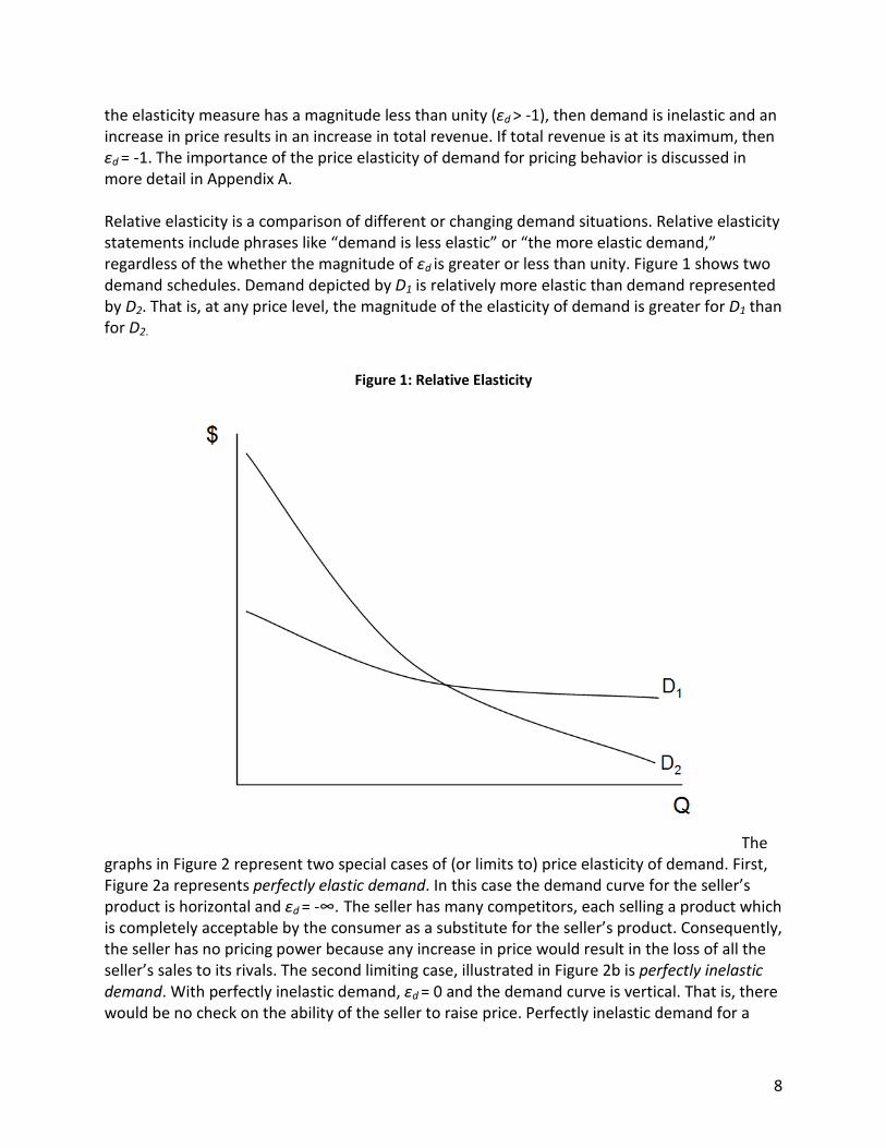
the elasticity measure has a magnitude less than unity (εd > -1), then demand is inelastic and an increase in price results in an increase in total revenue. If total revenue is at its maximum, then εd = -1. The importance of the price elasticity of demand for pricing behavior is discussed in more detail in Appendix A. Relative elasticity is a comparison of different or changing demand situations. Relative elasticity statements include phrases like “demand is less elastic” or “the more elastic demand,” regardless of the whether the magnitude of εd is greater or less than unity. Figure 1 shows two demand schedules. Demand depicted by D1 is relatively more elastic than demand represented by D2. That is, at any price level, the magnitude of the elasticity of demand is greater for D1 than for D2.

Figure 1: Relative Elasticity

The graphs in Figure 2 represent two special cases of (or limits to) price elasticity of demand. First, Figure 2a represents perfectly elastic demand. In this case the demand curve for the seller’s product is horizontal and εd = -∞. The seller has many competitors, each selling a product which is completely acceptable by the consumer as a substitute for the seller’s product. Consequently, the seller has no pricing power because any increase in price would result in the loss of all the seller’s sales to its rivals. The second limiting case, illustrated in Figure 2b is perfectly inelastic demand. With perfectly inelastic demand, εd = 0 and the demand curve is vertical. That is, there would be no check on the ability of the seller to raise price. Perfectly inelastic demand for a

9

seller’s good would require that the seller have no competitors and that the good be an absolute necessity at the observed quantities demanded.

Figure 2: Perfectly Elastic Demand and Perfectly Inelastic Demand

(a) (b) Perfectly Elastic Demand Curve Perfectly Inelastic Demand Curve

Both of these special cases are hypothetical cases that exist mainly in theory. Perfectly elastic demand may be approximately accurate when there are many sellers selling a commodity and there are low barriers to entry into and exit from the industry. Perfectly inelastic demand, on the other hand, is a more unrealistic extreme. Even a pure monopolist will face demand elasticity as consumers have ability to just consume less of the good as price rises.5

II.B. Household and Business Demand for Postal Services

Households use postal services for many reasons. These include personal correspondence, business purchases, bill payments, and the transfer of materials to other persons. The demands for these postal services by individuals are founded in the behavior of households as they choose how to save, or to spend incomes across the vast array of goods and services. Economists see the household’s objective as one of attaining the maximum satisfaction (also called utility) possible given an income or budget. Some household consumption of postal services, such as writing a personal letter, directly produces satisfaction. Other uses of postal services, such as paying a utility bill, do not produce satisfaction in and of themselves, but are intermediate goods used in the process of obtaining final consumption goods, such as air conditioning. To the extent that use of a postal service is an intermediate input, then the demand determinants and properties are derived from the

5 When we observe zero or positive own price elasticities empirically, as in the rolling coefficient analyses in Section IV, below, we would normally view those as examples of regression model “failure.” However, it is possible both that demands are highly inelastic over some ranges of prices and/or highly inelastic in the short run.

10

demand for the final product and are thus similar to the business demand for postal services discussed below.6 Businesses use postal services as inputs in the process of making and marketing their products. The business demands for postal services include direct mail (solicitation and advertising), merchandise transport, business and legal communications, and bill presentation. The demands for these postal services are founded in the behavior of businesses pursing their objectives. Consequently, the demand for an input of production is derived from the demand for the final product and also from the supply of other factors of production. This theory of derived demand, first developed by Alfred Marshall,7 typically assumes the business is an enterprise that produces and sells its product in an effort to achieve maximum profit. However, even if the firm is a not-for-profit enterprise pursuing some other objective, its demand for inputs is still derived from the final product market.8

II.C. Determinants of the Price Elasticity of Demand

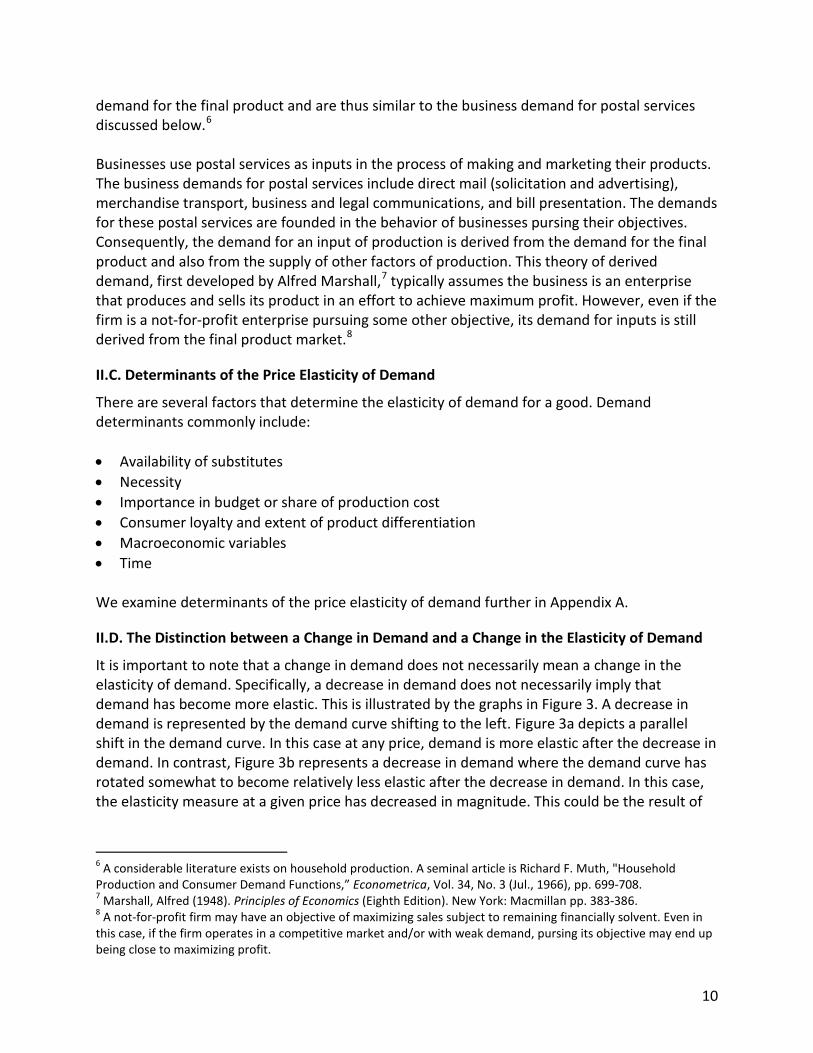
There are several factors that determine the elasticity of demand for a good. Demand determinants commonly include: • Availability of substitutes • Necessity • Importance in budget or share of production cost • Consumer loyalty and extent of product differentiation • Macroeconomic variables • Time We examine determinants of the price elasticity of demand further in Appendix A.

II.D. The Distinction between a Change in Demand and a Change in the Elasticity of Demand

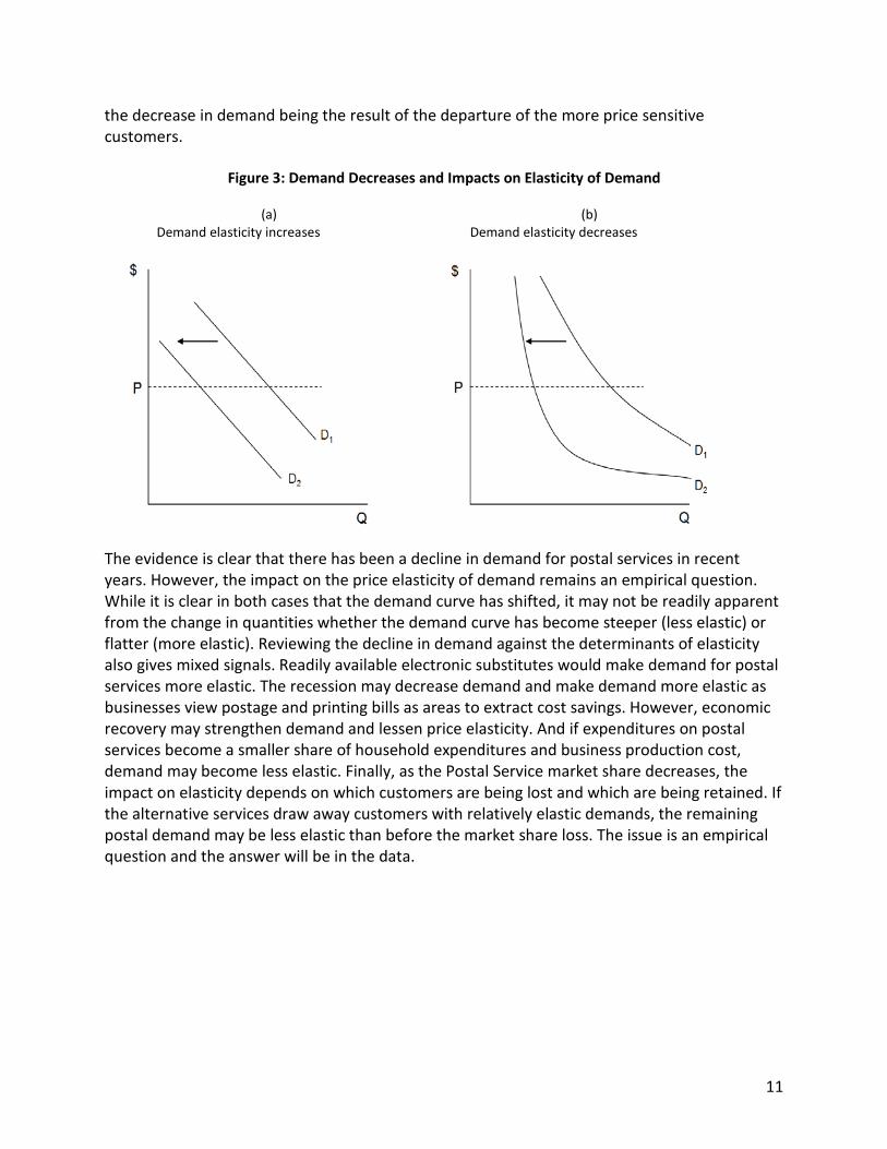
It is important to note that a change in demand does not necessarily mean a change in the elasticity of demand. Specifically, a decrease in demand does not necessarily imply that demand has become more elastic. This is illustrated by the graphs in Figure 3. A decrease in demand is represented by the demand curve shifting to the left. Figure 3a depicts a parallel shift in the demand curve. In this case at any price, demand is more elastic after the decrease in demand. In contrast, Figure 3b represents a decrease in demand where the demand curve has rotated somewhat to become relatively less elastic after the decrease in demand. In this case, the elasticity measure at a given price has decreased in magnitude. This could be the result of

6 A considerable literature exists on household production. A seminal article is Richard F. Muth, "Household Production and Consumer Demand Functions,” Econometrica, Vol. 34, No. 3 (Jul., 1966), pp. 699-708. 7 Marshall, Alfred (1948). Principles of Economics (Eighth Edition). New York: Macmillan pp. 383-386. 8 A not-for-profit firm may have an objective of maximizing sales subject to remaining financially solvent. Even in this case, if the firm operates in a competitive market and/or with weak demand, pursing its objective may end up being close to maximizing profit.

11

the decrease in demand being the result of the departure of the more price sensitive customers.

Figure 3: Demand Decreases and Impacts on Elasticity of Demand

(a) (b) Demand elasticity increases Demand elasticity decreases

The evidence is clear that there has been a decline in demand for postal services in recent years. However, the impact on the price elasticity of demand remains an empirical question. While it is clear in both cases that the demand curve has shifted, it may not be readily apparent from the change in quantities whether the demand curve has become steeper (less elastic) or flatter (more elastic). Reviewing the decline in demand against the determinants of elasticity also gives mixed signals. Readily available electronic substitutes would make demand for postal services more elastic. The recession may decrease demand and make demand more elastic as businesses view postage and printing bills as areas to extract cost savings. However, economic recovery may strengthen demand and lessen price elasticity. And if expenditures on postal services become a smaller share of household expenditures and business production cost, demand may become less elastic. Finally, as the Postal Service market share decreases, the impact on elasticity depends on which customers are being lost and which are being retained. If the alternative services draw away customers with relatively elastic demands, the remaining postal demand may be less elastic than before the market share loss. The issue is an empirical question and the answer will be in the data.

12

III. ECONOMETRIC ESTIMATION METHODS FOR POSTAL SERVICE DEMANDS

III.A. Postal Service Baseline Models

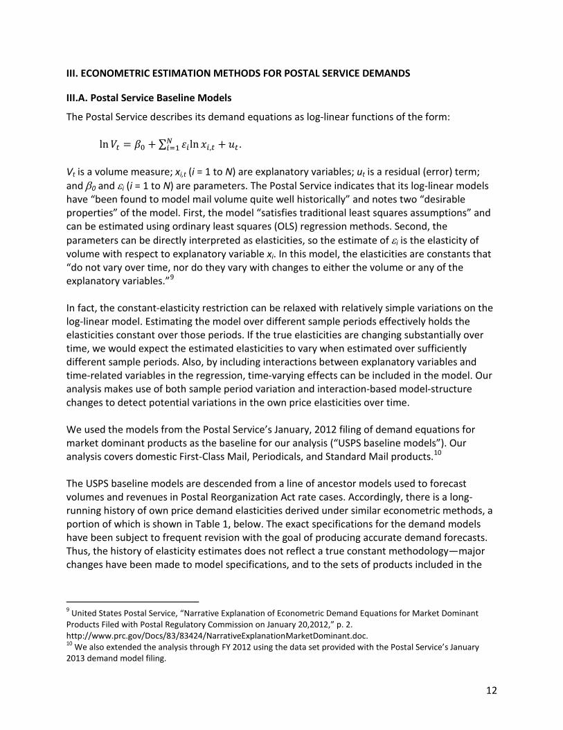
The Postal Service describes its demand equations as log-linear functions of the form: ln𝑉𝑡 = 𝛽0 + ∑ 𝜀𝑖ln 𝑥𝑖,𝑡𝑁

𝑖=1 + 𝑢𝑡. Vt is a volume measure; xi,t (i = 1 to N) are explanatory variables; ut is a residual (error) term; and β0 and εi (i = 1 to N) are parameters. The Postal Service indicates that its log-linear models have “been found to model mail volume quite well historically” and notes two “desirable properties” of the model. First, the model “satisfies traditional least squares assumptions” and can be estimated using ordinary least squares (OLS) regression methods. Second, the parameters can be directly interpreted as elasticities, so the estimate of εi is the elasticity of volume with respect to explanatory variable xi. In this model, the elasticities are constants that “do not vary over time, nor do they vary with changes to either the volume or any of the explanatory variables.”9 In fact, the constant-elasticity restriction can be relaxed with relatively simple variations on the log-linear model. Estimating the model over different sample periods effectively holds the elasticities constant over those periods. If the true elasticities are changing substantially over time, we would expect the estimated elasticities to vary when estimated over sufficiently different sample periods. Also, by including interactions between explanatory variables and time-related variables in the regression, time-varying effects can be included in the model. Our analysis makes use of both sample period variation and interaction-based model-structure changes to detect potential variations in the own price elasticities over time. We used the models from the Postal Service’s January, 2012 filing of demand equations for market dominant products as the baseline for our analysis (“USPS baseline models”). Our analysis covers domestic First-Class Mail, Periodicals, and Standard Mail products.10 The USPS baseline models are descended from a line of ancestor models used to forecast volumes and revenues in Postal Reorganization Act rate cases. Accordingly, there is a long-running history of own price demand elasticities derived under similar econometric methods, a portion of which is shown in Table 1, below. The exact specifications for the demand models have been subject to frequent revision with the goal of producing accurate demand forecasts. Thus, the history of elasticity estimates does not reflect a true constant methodology—major changes have been made to model specifications, and to the sets of products included in the

9 United States Postal Service, “Narrative Explanation of Econometric Demand Equations for Market Dominant Products Filed with Postal Regulatory Commission on January 20,2012,” p. 2. http://www.prc.gov/Docs/83/83424/NarrativeExplanationMarketDominant.doc. 10 We also extended the analysis through FY 2012 using the data set provided with the Postal Service’s January 2013 demand model filing.

13

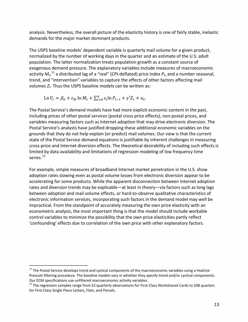
analysis. Nevertheless, the overall picture of the elasticity history is one of fairly stable, inelastic demands for the major market dominant products. The USPS baseline models’ dependent variable is quarterly mail volume for a given product, normalized by the number of working days in the quarter and an estimate of the U.S. adult population. The latter normalization treats population growth as a constant source of exogenous demand pressure. The explanatory variables include measures of macroeconomic activity Mt,11 a distributed lag of a “real” (CPI-deflated) price index Pt, and a number seasonal, trend, and “intervention” variables to capture the effects of other factors affecting mail volumes Zt. Thus the USPS baseline models can be written as: Ln𝑉𝑡 = 𝛽0 + 𝜀𝑀 ln𝑀𝑡 + ∑ 𝜀𝑖ln𝑃𝑡−𝑖4

𝑖=0 + 𝛾′𝑍𝑡 + 𝑢𝑡. The Postal Service’s demand models have had more explicit economic content in the past, including prices of other postal services (postal cross price effects), non-postal prices, and variables measuring factors such as Internet adoption that may drive electronic diversion. The Postal Service’s analysts have justified dropping these additional economic variables on the grounds that they do not help explain (or predict) mail volumes. Our view is that the current state of the Postal Service demand equations is justifiable by inherent challenges in measuring cross-price and Internet diversion effects. The theoretical desirability of including such effects is limited by data availability and limitations of regression modeling of low frequency time series.12 For example, simple measures of broadband Internet market penetration in the U.S. show adoption rates slowing even as postal volume losses from electronic diversion appear to be accelerating for some products. While the apparent disconnection between Internet adoption rates and diversion trends may be explicable—at least in theory—via factors such as long lags between adoption and mail volume effects, or hard-to-observe qualitative characteristics of electronic information services, incorporating such factors in the demand model may well be impractical. From the standpoint of accurately measuring the own price elasticity with an econometric analysis, the most important thing is that the model should include workable control variables to minimize the possibility that the own price elasticities partly reflect ‘confounding’ effects due to correlation of the own price with other explanatory factors.

11 The Postal Service develops trend and cyclical components of the macroeconomic variables using a Hodrick-Prescott filtering procedure. The baseline models vary in whether they specify trend and/or cyclical components. Our ECM specifications use unfiltered macroeconomic activity variables. 12 The regression samples range from 52 quarterly observations for First-Class Workshared Cards to 108 quarters for First-Class Single Piece Letters, Flats, and Parcels.

14

Table 1. Own Price Elasticity History

Class Subclass or Product Category 1990 1994 1997 2000 2001 2005 2006 2007 2008 2009 2010 2011 2012

First-Class Mail

Letters, Flats & Parcels (LFP) 0.245 0.188

Single Piece LFP 0.189 0.262 0.311 0.175 0.184 0.232 0.218 0.192 0.182 0.189

Single Piece Letters & Cards 0.090

Single Piece Flats 0.265

Workshared LFP 0.289 0.251 0.071 0.329 0.130 0.246 0.250 0.436 0.346 0.436

Workshared Letters, Flats, & Cards 0.392

Parcels 0.213

Postal Cards 1.242 0.248 0.168 0.761 0.808

Private Cards 1.242 0.985 0.944 0.860 1.157

Postcards 0.376

Single-Piece Postcards 0.258 0.110 0.117 0.397 0.249 0.063

Workshared Postcards 0.540 0.533 0.835 1.427 1.397 0.292

Periodicals

Regular Rate 0.291 0.145 0.143 0.148 0.166 0.193 0.294 0.245 0.260 0.082

Within County 0.546 0.395 0.530 0.142 0.157 0.235 0.141 0.165 0.152 0.207

Nonprofit 0.221 0.121 0.228 0.236

Classroom 1.305 0.994 1.178 0.407

Nonprofit &Classroom 0.092 0.237 0.212 0.258 0.330 0.276

Total 0.133 0.122 0.126

Standard Mail

Third Class Single Piece 0.476 0.484

Third Class Regular Bulk 0.624

Regular (Commercial non-ECR) 0.331 0.382 0.570 0.388 0.267 0.296 0.368 0.311 0.244 0.286 0.335 .0437

Enhanced Carrier Route (ECR) 0.662 0.598 0.808 0.770 1.093 1.079 0.771 0.911 0.839 0.727 0.782 .0704

Nonprofit Bulk/Nonprofit 0.258 0.442 0.136 0.162 0.230 0.319

Nonprofit 0.306 0.105 0.176 0.165 0.177 0.265 0.299

Nonprofit ECR 0.284 0.539 0.525 0.524 0.513 0.542 0.560 Source: Various PRC omnibus rate case and annual PAEA compliance filings. Elasticities are reported in absolute value.

15

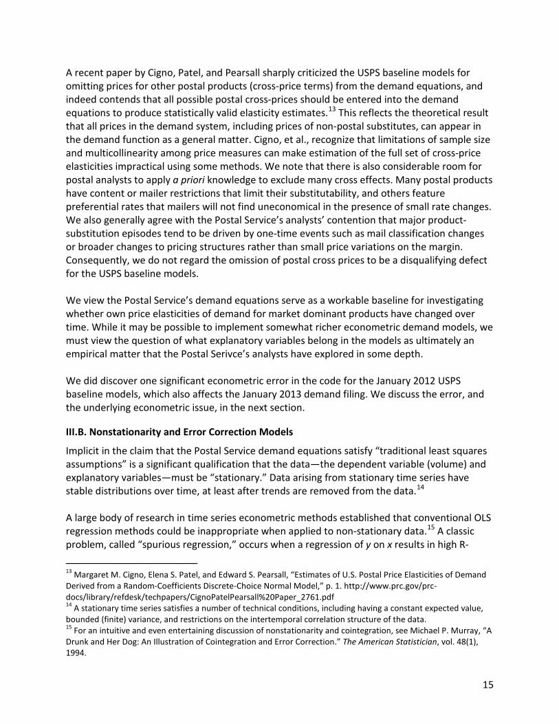
A recent paper by Cigno, Patel, and Pearsall sharply criticized the USPS baseline models for omitting prices for other postal products (cross-price terms) from the demand equations, and indeed contends that all possible postal cross-prices should be entered into the demand equations to produce statistically valid elasticity estimates.13 This reflects the theoretical result that all prices in the demand system, including prices of non-postal substitutes, can appear in the demand function as a general matter. Cigno, et al., recognize that limitations of sample size and multicollinearity among price measures can make estimation of the full set of cross-price elasticities impractical using some methods. We note that there is also considerable room for postal analysts to apply a priori knowledge to exclude many cross effects. Many postal products have content or mailer restrictions that limit their substitutability, and others feature preferential rates that mailers will not find uneconomical in the presence of small rate changes. We also generally agree with the Postal Service’s analysts’ contention that major product-substitution episodes tend to be driven by one-time events such as mail classification changes or broader changes to pricing structures rather than small price variations on the margin. Consequently, we do not regard the omission of postal cross prices to be a disqualifying defect for the USPS baseline models. We view the Postal Service’s demand equations serve as a workable baseline for investigating whether own price elasticities of demand for market dominant products have changed over time. While it may be possible to implement somewhat richer econometric demand models, we must view the question of what explanatory variables belong in the models as ultimately an empirical matter that the Postal Serivce’s analysts have explored in some depth. We did discover one significant econometric error in the code for the January 2012 USPS baseline models, which also affects the January 2013 demand filing. We discuss the error, and the underlying econometric issue, in the next section.

III.B. Nonstationarity and Error Correction Models

Implicit in the claim that the Postal Service demand equations satisfy “traditional least squares assumptions” is a significant qualification that the data—the dependent variable (volume) and explanatory variables—must be “stationary.” Data arising from stationary time series have stable distributions over time, at least after trends are removed from the data.14 A large body of research in time series econometric methods established that conventional OLS regression methods could be inappropriate when applied to non-stationary data.15 A classic problem, called “spurious regression,” occurs when a regression of y on x results in high R-

13 Margaret M. Cigno, Elena S. Patel, and Edward S. Pearsall, “Estimates of U.S. Postal Price Elasticities of Demand Derived from a Random-Coefficients Discrete-Choice Normal Model,” p. 1. http://www.prc.gov/prc-docs/library/refdesk/techpapers/CignoPatelPearsall%20Paper_2761.pdf 14 A stationary time series satisfies a number of technical conditions, including having a constant expected value, bounded (finite) variance, and restrictions on the intertemporal correlation structure of the data. 15 For an intuitive and even entertaining discussion of nonstationarity and cointegration, see Michael P. Murray, “A Drunk and Her Dog: An Illustration of Cointegration and Error Correction.” The American Statistician, vol. 48(1), 1994.

16

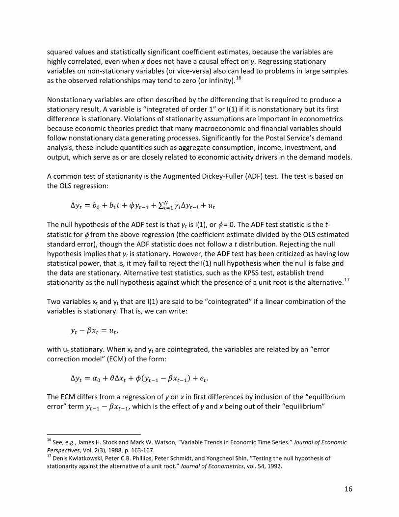
squared values and statistically significant coefficient estimates, because the variables are highly correlated, even when x does not have a causal effect on y. Regressing stationary variables on non-stationary variables (or vice-versa) also can lead to problems in large samples as the observed relationships may tend to zero (or infinity).16 Nonstationary variables are often described by the differencing that is required to produce a stationary result. A variable is “integrated of order 1” or I(1) if it is nonstationary but its first difference is stationary. Violations of stationarity assumptions are important in econometrics because economic theories predict that many macroeconomic and financial variables should follow nonstationary data generating processes. Significantly for the Postal Service’s demand analysis, these include quantities such as aggregate consumption, income, investment, and output, which serve as or are closely related to economic activity drivers in the demand models. A common test of stationarity is the Augmented Dickey-Fuller (ADF) test. The test is based on the OLS regression: Δ𝑦𝑡 = 𝑏0 + 𝑏1𝑡 + 𝜙𝑦𝑡−1 + ∑ 𝛾𝑖Δ𝑦𝑡−𝑖𝑁

𝑖=1 + 𝑢𝑡 The null hypothesis of the ADF test is that yt is I(1), or φ = 0. The ADF test statistic is the t-statistic for φ from the above regression (the coefficient estimate divided by the OLS estimated standard error), though the ADF statistic does not follow a t distribution. Rejecting the null hypothesis implies that yt is stationary. However, the ADF test has been criticized as having low statistical power, that is, it may fail to reject the I(1) null hypothesis when the null is false and the data are stationary. Alternative test statistics, such as the KPSS test, establish trend stationarity as the null hypothesis against which the presence of a unit root is the alternative.17 Two variables xt and yt that are I(1) are said to be “cointegrated” if a linear combination of the variables is stationary. That is, we can write:

𝑦𝑡 − 𝛽𝑥𝑡 = 𝑢𝑡, with ut stationary. When xt and yt are cointegrated, the variables are related by an “error correction model” (ECM) of the form:

∆𝑦𝑡 = 𝛼0 + 𝜃∆𝑥𝑡 + 𝜙(𝑦𝑡−1 − 𝛽𝑥𝑡−1) + 𝑒𝑡. The ECM differs from a regression of y on x in first differences by inclusion of the “equilibrium error” term 𝑦𝑡−1 − 𝛽𝑥𝑡−1, which is the effect of y and x being out of their “equilibrium”

16 See, e.g., James H. Stock and Mark W. Watson, “Variable Trends in Economic Time Series.” Journal of Economic Perspectives, Vol. 2(3), 1988, p. 163-167. 17 Denis Kwiatkowski, Peter C.B. Phillips, Peter Schmidt, and Yongcheol Shin, “Testing the null hypothesis of stationarity against the alternative of a unit root.” Journal of Econometrics, vol. 54, 1992.

17

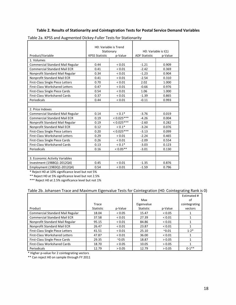
relationship. The differenced variables and the equilibrium error term are all stationary, so the ECM can be estimated via least squares regression methods.18 The Postal Service’s analysts clearly have been aware of the potential for nonstationarity of the demand data. The demand model filings report ADF test results for the volume variables employed in the demand models, and for the demand models’ residuals. The reported test results have rejected the null hypotheses of nonstationarity, and thus ostensibly justified the use of traditional regression methods for stationary time series. However, while reviewing the Postal Service’s estimation code, we found major errors in the implementation of the ADF tests. The econometric code filed in January 2012 had errors in both the implementation of the ADF regression and the calculation of the ADF t-statistic. The code in the January 2013 filing corrected the regression specification but not the t-statistic calculation. We computed the results of ADF tests for the volumes, unfiltered economic activity variables, and prices in the demand equations we studied, based on a corrected version of the ADF test implemented in the Postal Service’s demand model filing.19 We also conducted a set of parallel tests using the KPSS statistic. We used the Johansen trace statistic to test for the presence of cointegtration where the stationarity testing indicated the data to be I(1).20 Results are provided in Table 2, below. The ADF tests uniformly fail to reject the null hypothesis of nonstationarity for the volumes of market dominant products and for the economic activity variables. Results for prices are mixed. The ADF tests reject the I(1) null hypothesis in favor of stationarity at the 10 percent significance level (or better) for Standard Mail prices except for Nonprofit Standard Mail Regular (non-ECR). Additionally, the ADF statistics for Periodicals, First-Class Single Piece Letters, and First-Class Workshared Cards prices are very close to the 10 percent critical values. The KPSS test statistics also reject the null of trend stationarity for the volumes and economic activity variables; they also tend to reject trend stationarity for the price variables.

18 Variations on the ECM include seasonal differencing (sometimes applied to quarterly data, where the SPLY difference yt - yt-4 may be more economically significant than the first difference), and the inclusion of stationary regressors and additional lags of the I(1) variables. The ECM is a type of autoregressive model that also can be used to analyze stationary data. 19 The volumes and prices were transformed, and natural logarithms taken of the transformed variables, as in the econometric demand models. We tested the unfiltered economic activity variables in natural logarithms. 20 S. Johansen, Likelihood-Based Inference in Cointegrated Vector Autoregressive Models. Oxford University Press, 1995, chapters 11-12.

18

Table 2. Results of Stationarity and Cointegtration Tests for Postal Service Demand Variables

Table 2a. KPSS and Augmented Dickey-Fuller Tests for Stationarity

H0: Variable is Trend

Stationary H0: Variable is I(1) Product/Variable KPSS Statistic p-Value ADF Statistic p-Value 1. Volumes Commercial Standard Mail Regular 0.44 < 0.01 -1.21 0.909 Commercial Standard Mail ECR 0.41 < 0.01 -2.42 0.369 Nonprofit Standard Mail Regular 0.34 < 0.01 -1.23 0.904 Nonprofit Standard Mail ECR 0.41 < 0.01 -2.54 0.310 First-Class Single Piece Letters 0.70 < 0.01 2.02 1.000 First-Class Workshared Letters 0.47 < 0.01 -0.66 0.976 First-Class Single Piece Cards 0.54 < 0.01 1.06 1.000 First-Class Workshared Cards 0.37 < 0.01 -1.39 0.865 Periodicals 0.44 < 0.01 -0.11 0.993 2. Price Indexes Commercial Standard Mail Regular 0.14 < 0.1* -3.76 0.019 Commercial Standard Mail ECR 0.19 < 0.025*** -4.26 0.004 Nonprofit Standard Mail Regular 0.19 < 0.025*** -2.60 0.282 Nonprofit Standard Mail ECR 0.12 < 0.1* -3.24 0.076 First-Class Single Piece Letters 0.20 < 0.025*** -3.13 0.099 First-Class Workshared Letters 0.29 < 0.01 -2.24 0.465 First-Class Single Piece Cards 0.26 < 0.01 -2.09 0.554 First-Class Workshared Cards 0.13 < 0.1* -3.03 0.123 Periodicals 0.16 < 0.05** -3.01 0.130 3. Economic Activity Variables Investment (1988Q1-2012Q4) 0.45 < 0.01 -1.35 0.876 Employment (1983Q1-2012Q4) 0.54 < 0.01 -1.59 0.796 * Reject H0 at 10% significance level but not 5% ** Reject H0 at 5% significance level but not 2.5% *** Reject H0 at 2.5% significance level but not 1%

Table 2b. Johansen Trace and Maximum Eigenvalue Tests for Cointegration (H0: Cointegrating Rank is 0)

Product Trace

Statistic p-Value

Max Eigenvalue

Statistic p-Value

Estimated # of

cointegrating vectors

Commercial Standard Mail Regular 18.04 < 0.05 15.47 < 0.05 1 Commercial Standard Mail ECR 37.58 < 0.01 27.39 < 0.01 1 Nonprofit Standard Mail Regular 95.15 < 0.01 84.86 < 0.01 1 Nonprofit Standard Mail ECR 26.47 < 0.01 23.87 < 0.01 1 First-Class Single Piece Letters 41.51 < 0.01 25.10 ~0.01 1-2* First-Class Workshared Letters 47.87 < 0.01 36.00 < 0.01 1 First-Class Single Piece Cards 29.35 ~0.05 18.87 > 0.05 1 First-Class Workshared Cards 18.70 < 0.05 10.05 > 0.05 1 Periodicals 12.79 > 0.05 12.79 > 0.05 0-1**

* Higher p-value for 2 cointegrating vectors ** Can reject H0 on sample through FY 2011

19

The result that the price variables are not trend stationary is somewhat counterintuitive. Over the long run, indexes of U.S. postal prices have not tended to diverge significantly from the Consumer Price Index (CPI). To the extent the fixed-weight price indexes for the postal products are proportional to CPI, then their ratio—the “real” price—would be stationary. The CPI price caps under PAEA would be expected to impose such a relationship for the product aggregates where the caps apply; pre-PAEA pricing policies may have served to limit divergence between some Postal Service rates and CPI as well.21 On the other hand, pre-PAEA price adjustments led to occasional large changes in “real” prices, and the PAEA caps do not necessarily constrain prices at the product level (within classes) to CPI. The Johansen trace tests showed the volumes, prices, and economic activity variables to be cointegrated for the products under study, generally with a single cointegrating vector. The main exception was Periodicals, where the trace test could not reject the hypothesis of no cointegration for the full sample (1993 Q1-2012 Q4) at a p-value of 0.05, though other tests showed the presence of a cointegrating vector.22 Given the results in Table 2, we conducted our analysis using both a modified USPS baseline model and ECM implementations of the Postal Service demand equations. Because the USPS baseline models have been the source of official demand elasticities, the behavior of those models may still be of interest. Additionally, since there is much less experience with ECM specifications for USPS demand models than with the USPS baseline models, understanding the current models’ (mis)behavior under alternative samples and other specification changes may provide a useful yardstick for evaluating the performance of the ECMs.

III.C. Modified USPS Baseline Demand Models

While the Postal Service demand models are based on log-linear demand functions, the specific econometric implementation of the models introduce some nonlinearities and multi-step estimation procedures. To avoid some computational issues with the rolling and recursive parameter analyses, we employed one-step linear models that yield very similar results to the Postal Service’s filed models. One set of changes concerns the distributed lag of price variables on the right-hand side of the regression equation. Since the current and lagged prices are highly intercorrelated, unconstrained estimates of the coefficients for the distributed lag are often highly volatile;

21 The lower frequency of rate cases under the Postal Reorganization Act tended to result in larger nominal increases than the more frequent but smaller rate changes under the PAEA price cap system, but the effects of inflationary erosion of the real value of the increases leave relatively little long-run trend in the real fixed-weight price indexes for the products under study in either the PRA or PAEA periods. A recent study found that UK postal prices deflated by the Retail Price Index (RPI) were stationary or I(0). The study noted that UK postal prices have subject to an RPI-X price cap since 2003. See Leticia Veruete-McKay, Soterios Soteri, John Nankervis, and Frank Rodriguez, “Letter Traffic Demand in the UK: An Analysis by Product and Envelope Content Type,” Review of Network Economics, Vol. 10(3), September 2011. 22 These included the Johansen maximum eigenvalue test and the trace test performed on the subset of data through FY 2011.

20

anomalous results such as large positive elasticities are not uncommon. We used a polynomial distributed lag (PDL) model, which constrains the coefficients of the distributed lag to fall on a second-order (quadratic) polynomial. The PDL model can be implemented as a set of linear constraints on the demand model parameters. The Postal Service’s approach uses a method which does not require the coefficients to fall exactly on the lag polynomial (called the Shiller “smoothness prior” method), but which requires setting a parameter in advance of the model estimation. Postal Service analysts had previously reported that the Shiller method and the PDL model produce similar results.23 Additionally, we use four lags of the price index variable for all products. In some cases, the Postal Service’s baseline models constrain the elasticities to zero for certain lags. While the criteria for lag selection are not explained in the Postal Service’s recent filings, we expect that the primary motivation was to avoid cases where the elasticities for certain lags had the “wrong” sign. In a number of cases, we found that the estimated elasticities for lags that were set to zero in the Postal Service models were not anomalous. The other change concerns nonlinear “interventions” included in the demand models for some (but not all) products. The interventions are included in the models to reflect the effects of exogenous determinants of demand that are not otherwise measured, such as electronic diversion effects. The interventions generally take the form: 𝐼𝑡 = 𝜔0𝑃𝑡 + 𝜔1(𝑃𝑡−1 + 𝛿𝑃𝑡−2 + 𝛿2𝑃𝑡−3 + ⋯ ) + 𝜔2𝑆𝑡 + 𝜔3𝑇𝑡.24 It is linear in the variables Pt, St, and Tt, but nonlinear in the parameters due to the coefficient δ on the lagged pulse terms. We used the Postal Service’s estimates of δ to compute “decay” variables: 𝐷𝑡 = 𝑃𝑡−1 + 𝛿𝑃𝑡−2 + 𝛿2𝑃𝑡−3 + ⋯ and we estimated the other transfer function parameters using: 𝐼𝑡 = 𝜔0𝑃𝑡 + 𝜔1𝐷𝑡 + 𝜔2𝑆𝑡 + 𝜔3𝑇𝑡. In some models, notably for single piece and workshared First-Class Mail letters, flats, and parcels, the interventions in the Postal Service models assume (at least) 𝜔1 = 0, in which case our implementation is not restricted relative to the Postal Service baseline models. Finally, the Postal Service models incorporate a Cochrane-Orcutt transformation of the data to adjust for autocorrelation of the regression residuals. This involves obtaining an estimate of the residual autocorrelation coefficient from an OLS regression, transforming the data, and re-running the regression using the transformed data. Since the transformation is not required to obtain consistent coefficient estimates, we omitted it. However, standard variance formulas are

23 Postal Rate Commission, Docket No. R90-1, Direct Testimony of George S. Tolley (USPS-T-2), pages I-43 to I-46. 24 United States Postal Service, “Narrative Explanation of Econometric Demand Equations for Market Dominant Products Filed with Postal Regulatory Commission on January 20,2012,” p. 11.

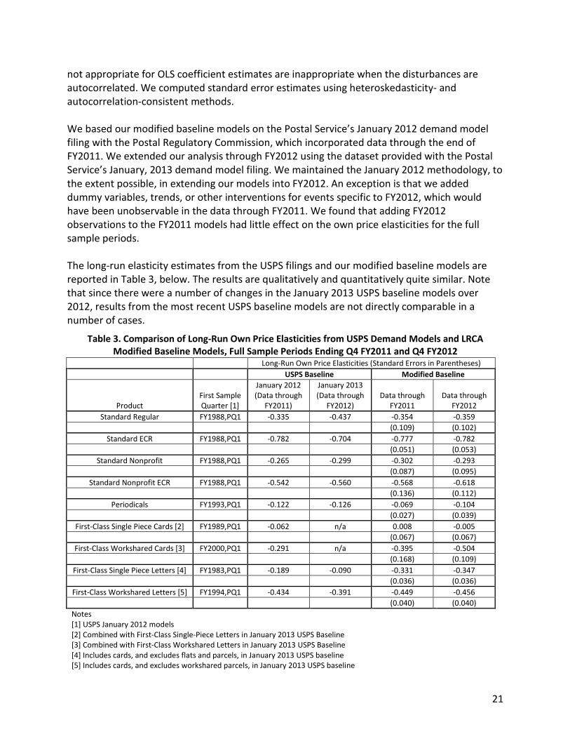
21

not appropriate for OLS coefficient estimates are inappropriate when the disturbances are autocorrelated. We computed standard error estimates using heteroskedasticity- and autocorrelation-consistent methods. We based our modified baseline models on the Postal Service’s January 2012 demand model filing with the Postal Regulatory Commission, which incorporated data through the end of FY2011. We extended our analysis through FY2012 using the dataset provided with the Postal Service’s January, 2013 demand model filing. We maintained the January 2012 methodology, to the extent possible, in extending our models into FY2012. An exception is that we added dummy variables, trends, or other interventions for events specific to FY2012, which would have been unobservable in the data through FY2011. We found that adding FY2012 observations to the FY2011 models had little effect on the own price elasticities for the full sample periods. The long-run elasticity estimates from the USPS filings and our modified baseline models are reported in Table 3, below. The results are qualitatively and quantitatively quite similar. Note that since there were a number of changes in the January 2013 USPS baseline models over 2012, results from the most recent USPS baseline models are not directly comparable in a number of cases.

Table 3. Comparison of Long-Run Own Price Elasticities from USPS Demand Models and LRCA Modified Baseline Models, Full Sample Periods Ending Q4 FY2011 and Q4 FY2012

Long-Run Own Price Elasticities (Standard Errors in Parentheses) USPS Baseline Modified Baseline

Product First Sample Quarter [1]

January 2012 (Data through

FY2011)

January 2013 (Data through

FY2012) Data through

FY2011 Data through

FY2012 Standard Regular FY1988,PQ1 -0.335 -0.437 -0.354 -0.359

(0.109) (0.102) Standard ECR FY1988,PQ1 -0.782 -0.704 -0.777 -0.782

(0.051) (0.053) Standard Nonprofit FY1988,PQ1 -0.265 -0.299 -0.302 -0.293

(0.087) (0.095) Standard Nonprofit ECR FY1988,PQ1 -0.542 -0.560 -0.568 -0.618

(0.136) (0.112) Periodicals FY1993,PQ1 -0.122 -0.126 -0.069 -0.104

(0.027) (0.039) First-Class Single Piece Cards [2] FY1989,PQ1 -0.062 n/a 0.008 -0.005

(0.067) (0.067) First-Class Workshared Cards [3] FY2000,PQ1 -0.291 n/a -0.395 -0.504

(0.168) (0.109) First-Class Single Piece Letters [4] FY1983,PQ1 -0.189 -0.090 -0.331 -0.347

(0.036) (0.036) First-Class Workshared Letters [5] FY1994,PQ1 -0.434 -0.391 -0.449 -0.456

(0.040) (0.040) Notes [1] USPS January 2012 models [2] Combined with First-Class Single-Piece Letters in January 2013 USPS Baseline [3] Combined with First-Class Workshared Letters in January 2013 USPS Baseline [4] Includes cards, and excludes flats and parcels, in January 2013 USPS baseline [5] Includes cards, and excludes workshared parcels, in January 2013 USPS baseline

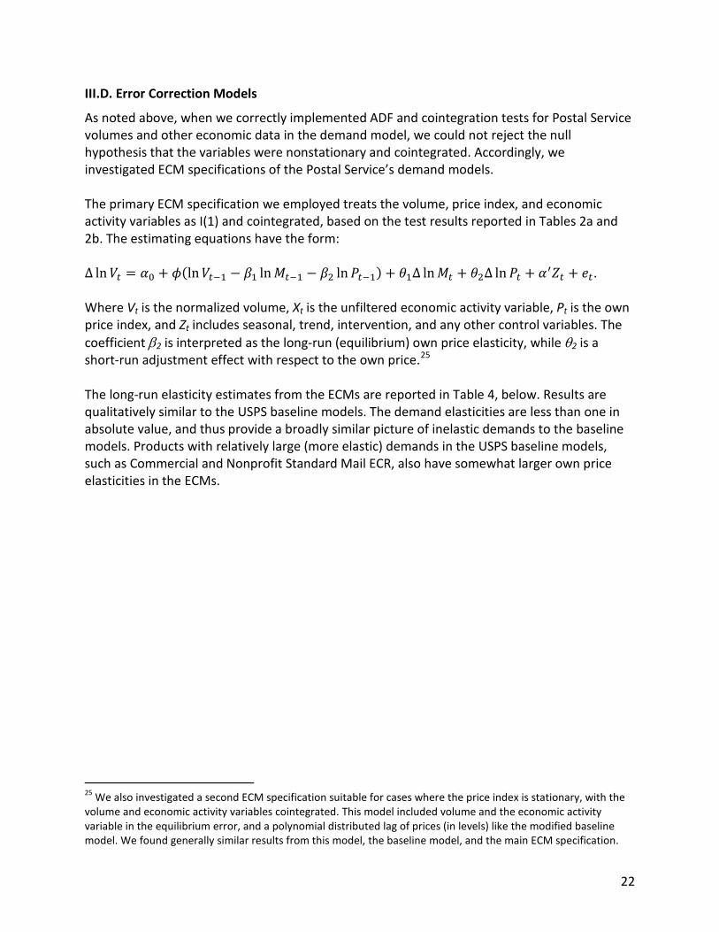
22

III.D. Error Correction Models

As noted above, when we correctly implemented ADF and cointegration tests for Postal Service volumes and other economic data in the demand model, we could not reject the null hypothesis that the variables were nonstationary and cointegrated. Accordingly, we investigated ECM specifications of the Postal Service’s demand models. The primary ECM specification we employed treats the volume, price index, and economic activity variables as I(1) and cointegrated, based on the test results reported in Tables 2a and 2b. The estimating equations have the form: Δ ln𝑉𝑡 = 𝛼0 + 𝜙(ln𝑉𝑡−1 − 𝛽1 ln𝑀𝑡−1 − 𝛽2 ln𝑃𝑡−1) + 𝜃1Δ ln𝑀𝑡 + 𝜃2Δ ln𝑃𝑡 + 𝛼′𝑍𝑡 + 𝑒𝑡. Where Vt is the normalized volume, Xt is the unfiltered economic activity variable, Pt is the own price index, and Zt includes seasonal, trend, intervention, and any other control variables. The coefficient β2 is interpreted as the long-run (equilibrium) own price elasticity, while θ2 is a short-run adjustment effect with respect to the own price.25 The long-run elasticity estimates from the ECMs are reported in Table 4, below. Results are qualitatively similar to the USPS baseline models. The demand elasticities are less than one in absolute value, and thus provide a broadly similar picture of inelastic demands to the baseline models. Products with relatively large (more elastic) demands in the USPS baseline models, such as Commercial and Nonprofit Standard Mail ECR, also have somewhat larger own price elasticities in the ECMs.

25 We also investigated a second ECM specification suitable for cases where the price index is stationary, with the volume and economic activity variables cointegrated. This model included volume and the economic activity variable in the equilibrium error, and a polynomial distributed lag of prices (in levels) like the modified baseline model. We found generally similar results from this model, the baseline model, and the main ECM specification.

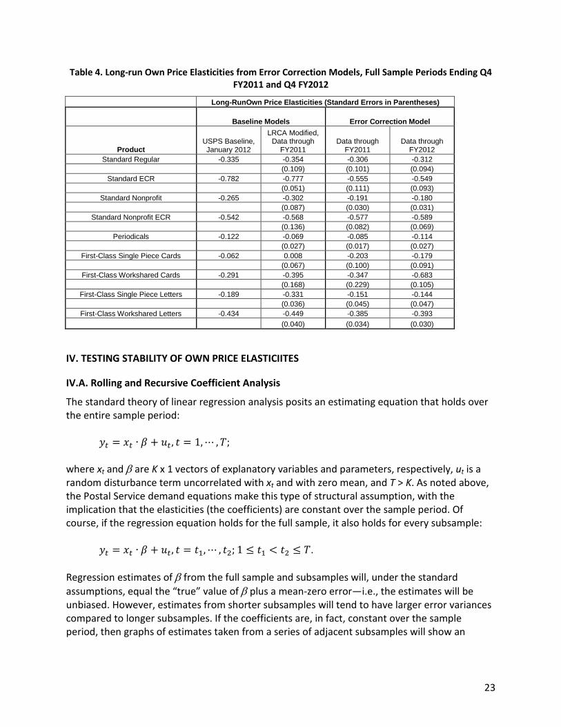
23

Table 4. Long-run Own Price Elasticities from Error Correction Models, Full Sample Periods Ending Q4 FY2011 and Q4 FY2012

Long-RunOwn Price Elasticities (Standard Errors in Parentheses)

Baseline Models Error Correction Model

Product USPS Baseline, January 2012

LRCA Modified, Data through

FY2011 Data through

FY2011 Data through

FY2012 Standard Regular -0.335 -0.354 -0.306 -0.312

(0.109) (0.101) (0.094) Standard ECR -0.782 -0.777 -0.555 -0.549

(0.051) (0.111) (0.093) Standard Nonprofit -0.265 -0.302 -0.191 -0.180

(0.087) (0.030) (0.031) Standard Nonprofit ECR -0.542 -0.568 -0.577 -0.589

(0.136) (0.082) (0.069) Periodicals -0.122 -0.069 -0.085 -0.114

(0.027) (0.017) (0.027) First-Class Single Piece Cards -0.062 0.008 -0.203 -0.179

(0.067) (0.100) (0.091) First-Class Workshared Cards -0.291 -0.395 -0.347 -0.683

(0.168) (0.229) (0.105) First-Class Single Piece Letters -0.189 -0.331 -0.151 -0.144

(0.036) (0.045) (0.047) First-Class Workshared Letters -0.434 -0.449 -0.385 -0.393

(0.040) (0.034) (0.030)

IV. TESTING STABILITY OF OWN PRICE ELASTICIITES

IV.A. Rolling and Recursive Coefficient Analysis

The standard theory of linear regression analysis posits an estimating equation that holds over the entire sample period: 𝑦𝑡 = 𝑥𝑡 ∙ 𝛽 + 𝑢𝑡, 𝑡 = 1,⋯ ,𝑇; where xt and β are K x 1 vectors of explanatory variables and parameters, respectively, ut is a random disturbance term uncorrelated with xt and with zero mean, and T > K. As noted above, the Postal Service demand equations make this type of structural assumption, with the implication that the elasticities (the coefficients) are constant over the sample period. Of course, if the regression equation holds for the full sample, it also holds for every subsample: 𝑦𝑡 = 𝑥𝑡 ∙ 𝛽 + 𝑢𝑡, 𝑡 = 𝑡1,⋯ , 𝑡2; 1 ≤ 𝑡1 < 𝑡2 ≤ 𝑇. Regression estimates of β from the full sample and subsamples will, under the standard assumptions, equal the “true” value of β plus a mean-zero error—i.e., the estimates will be unbiased. However, estimates from shorter subsamples will tend to have larger error variances compared to longer subsamples. If the coefficients are, in fact, constant over the sample period, then graphs of estimates taken from a series of adjacent subsamples will show an

24

absence of a trend, since the estimates will be a constant (the “true” parameter value) plus noise. The noise term will tend to have a larger standard error for shorter subsamples. “Rolling” and “recursive” coefficient analyses employ coefficient estimates from sequences of adjacent subsamples to investigate the stability of regression coefficients. The methods differ in the sequences of subsamples, and have advantages and disadvantages in identifying certain types of changes to the coefficients. In the “rolling” analysis, the first subsample begins at period 1 and ends at period T0, where K<T0<T. T0 is sometimes called the “window” length for the rolling analysis. The second subsample consists of the T0 observations from period 2 to period T0+1, and so on, until the final subsample of T0 observations ends in period T. The “recursive” analysis starts with the first T0 observations, like the rolling analysis, but subsequent subsamples do not drop the early observations. Thus the second subsample is from period 1 to period T0+1, and so on, until the last recursive subsample is the full sample from period 1 to period T. The recursive analysis shows the effect of adding observations to the end of subsequent samples, and ends with the full-sample estimate. Finally, a “reverse recursive” analysis shows the effects of dropping observations from the start of the full sample period. It starts with the full sample t=1,…,T, and drops early observations from subsequent subsamples, so that the second subsample is from period 2 to period T, and the last subsample is estimated over the final window of length T0 ending at T—i.e., the final subsample from the rolling analysis. Rolling and reverse recursive analysis will tend to be more sensitive to changes in the coefficients in later time periods, compared to the recursive analysis, since later rolling and reverse recursive subsamples drop observations from early in the sample that might reflect a different underlying model structure. However, the estimates from rolling subsamples will tend to be “noisier” than the longer subsamples for the recursive analysis as the shorter sample periods compared to the recursive analysis will tend to increase the sampling variance of the coefficient estimates. Conversely, retaining earlier data tends to reduce the variance of the coefficient errors in longer recursive subsamples (which approach the full sample period), but may attenuate the effects of structural changes. All three methods are limited in that the shortest subsample that can be estimated is K+1 periods, where K is the number of explanatory variables in the model. In practice, the shortest subsamples that produce reasonable results may be much longer. If a regression model using quarterly data has 19 explanatory variables, then the minimum sample window is 20 quarters, or five years’ worth of data. This may not be sufficient to draw out changes that may have occurred near the end of the full sample period. Indeed, the USPS baseline models typically have upwards of 20 explanatory variables, most of which are seasonal, trend, and intervention terms. We ran the rolling and recursive analysis using windows of 40 and 60 quarters. We found some elasticity estimates using 40-quarter sample windows to be highly volatile, though the recursive coefficient analyses showed relatively stable elasticities using both the modified USPS baseline models and ECM specifications.

25

IV.B. Results of Rolling and Recursive Parameter Analysis

The rolling and recursive analyses of the USPS baseline and ECM demand model specifications show some model instability over some rolling subsamples, while the recursive analysis shows relatively stable own price elasticities as the sample periods are lengthened. With a few exceptions, most of the instability of the elasticities in the rolling samples is in the direction of zero elasticity rather than larger elasticities.

IV.B.1. Commercial Standard Mail Regular

Figures 4a and 4b show long-run elasticities for Commercial Standard Mail Regular from rolling and recursive analysis using the modified USPS baseline and the ECM specification, respectively. In these graphs (and similar figures for other products), we show the end period for the rolling and recursive samples. This helps identify whether apparent trend breaks correspond with the inclusion of data from periods of interest such as the Great Recession.26 In both models, the own price elasticities from nearly all of the rolling samples are smaller than in the recursive samples. This indicates that including older observations does not necessarily result in less elastic measured demands; in this case, the older data appear to be keeping the measured elasticities larger than they would be with more recent samples. The 60-quarter rolling samples through the sample ending in FY2009 quarter 1 are mostly between about -0.15 and -0.25.27 Beginning with the sample including FY2009 quarter 2—i.e., quarter 1 of calendar 2009, the quarter following severe financial-market disruptions prior to the 2008 election—the rolling samples jump towards zero, and mostly stay in the vicinity of zero or produce “wrong sign” elasticities. However, the 40-quarter rolling samples show increased volatility prior to the onset of the recession. The recursive samples are much more stable over time in all models, though a shift to smaller elasticities at FY2009 quarter 2 is still visible in the graphs. Cumulative sum (CUSUM) test indicate a possible structural break in both the baseline and ECM models, though the results are not statistically significant. The timing of the shifts in the Commercial Standard Mail Regular elasticities could reflect uncontrolled effects of the Great Recession. The January 2012 USPS baseline model includes a nonlinear intervention variable to capture Great Recession effects on volume. However, the start period for the intervention is FY2008 quarter 2, so the intervention variable does not account for the worsening recession in FY2009.28 Another possible factor is that the included macroeconomic activity variable, investment, has diverged from Commercial Standard Mail Regular volumes in the recovery.

26 Note that the scales of the graphs are the same for each product, but owing to differences in the levels and variability of the results, not across products. 27 A reverse recursive analysis shows that starting the sample slightly later than the FY1988 Q1 start of the sample for the USPS baseline model would also result in a smaller elasticity for Commercial Standard Mail Regular. 28 The NBER calendar date for the start of the recession was December, 2007, which is in quarter 1 of the 2008 Postal Service fiscal year.

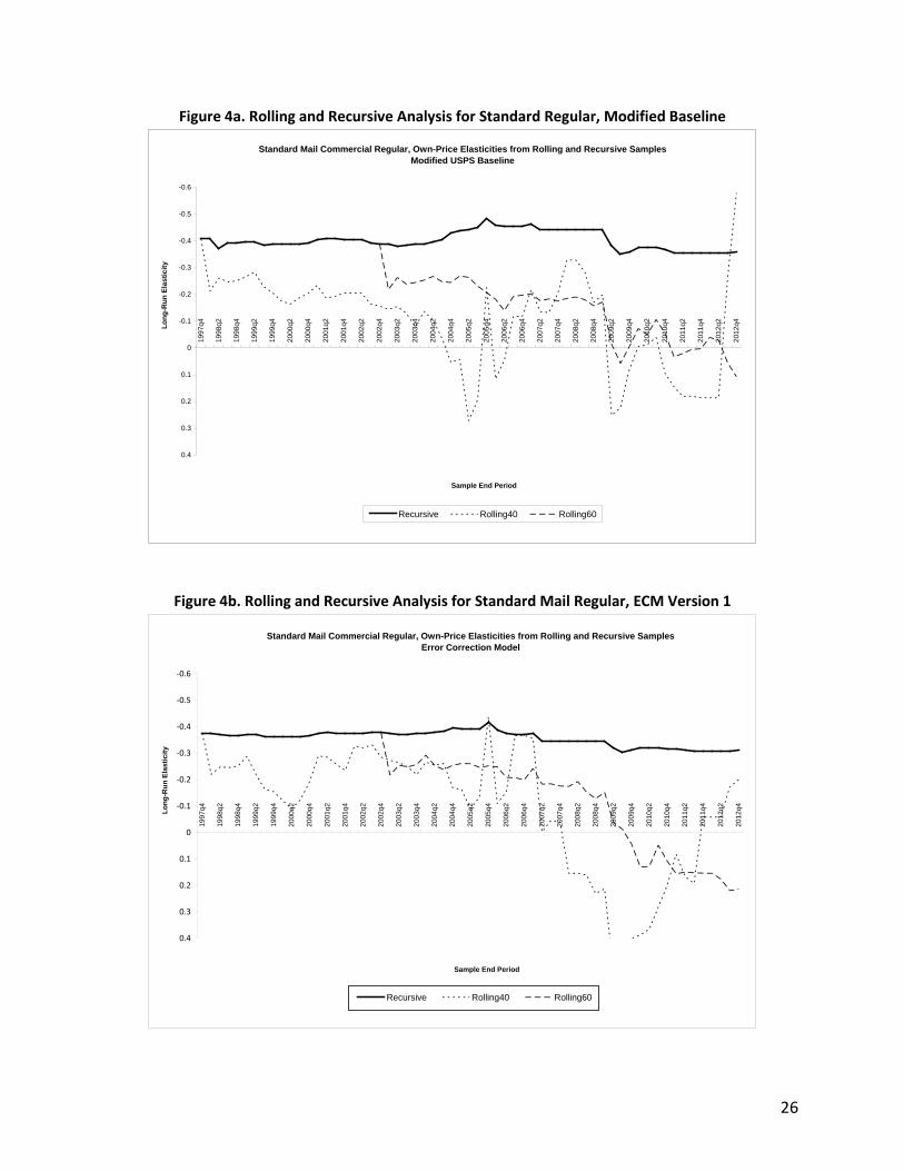
26

Figure 4a. Rolling and Recursive Analysis for Standard Regular, Modified Baseline

Figure 4b. Rolling and Recursive Analysis for Standard Mail Regular, ECM Version 1

Standard Mail Commercial Regular, Own-Price Elasticities from Rolling and Recursive SamplesModified USPS Baseline

-0.6

-0.5

-0.4

-0.3

-0.2

-0.1

0

0.1

0.2

0.3

0.4

1997

q4

1998

q2

1998

q4

1999

q2

1999

q4

2000

q2

2000

q4

2001

q2

2001

q4

2002

q2

2002

q4

2003

q2

2003

q4

2004

q2

2004

q4

2005

q2

2005

q4

2006

q2

2006

q4

2007

q2

2007

q4

2008

q2

2008

q4

2009

q2

2009

q4

2010

q2

2010

q4

2011

q2

2011

q4

2012

q2

2012

q4

Sample End Period

Long

-Run

Ela

stic

ity

Recursive Rolling40 Rolling60

Standard Mail Commercial Regular, Own-Price Elasticities from Rolling and Recursive SamplesError Correction Model

-0.6

-0.5

-0.4

-0.3

-0.2

-0.1

0

0.1

0.2

0.3

0.4

1997

q4

1998

q2

1998

q4

1999

q2

1999

q4

2000

q2

2000

q4

2001

q2

2001

q4

2002

q2

2002

q4

2003

q2

2003

q4

2004

q2

2004

q4

2005

q2

2005

q4

2006

q2

2006

q4

2007

q2

2007

q4

2008

q2

2008

q4

2009

q2

2009

q4

2010

q2

2010

q4

2011

q2

2011

q4

2012

q2

2012

q4

Sample End Period

Long

-Run

Ela

stic

ity

Recursive Rolling40 Rolling60

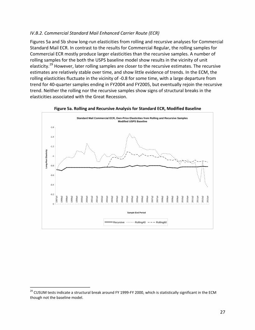
27

IV.B.2. Commercial Standard Mail Enhanced Carrier Route (ECR)

Figures 5a and 5b show long-run elasticities from rolling and recursive analyses for Commercial Standard Mail ECR. In contrast to the results for Commercial Regular, the rolling samples for Commercial ECR mostly produce larger elasticities than the recursive samples. A number of rolling samples for the both the USPS baseline model show results in the vicinity of unit elasticity.29 However, later rolling samples are closer to the recursive estimates. The recursive estimates are relatively stable over time, and show little evidence of trends. In the ECM, the rolling elasticities fluctuate in the vicinity of -0.8 for some time, with a large departure from trend for 40-quarter samples ending in FY2004 and FY2005, but eventually rejoin the recursive trend. Neither the rolling nor the recursive samples show signs of structural breaks in the elasticities associated with the Great Recession.

Figure 5a. Rolling and Recursive Analysis for Standard ECR, Modified Baseline

29 CUSUM tests indicate a structural break around FY 1999-FY 2000, which is statistically significant in the ECM though not the baseline model.

Standard Mail Commercial ECR, Own-Price Elasticities from Rolling and Recursive Samples Modified USPS Baseline

-1.6

-1.4

-1.2

-1

-0.8

-0.6

-0.4

-0.2

0

1997

q4

1998

q2

1998

q4

1999

q2

1999

q4

2000

q2

2000

q4

2001

q2

2001

q4

2002

q2

2002

q4

2003

q2

2003

q4

2004

q2

2004

q4

2005

q2

2005

q4

2006

q2

2006

q4

2007

q2

2007

q4

2008

q2

2008

q4

2009

q2

2009

q4

2010

q2

2010

q4

2011

q2

2011

q4

2012

q2

2012

q4

Sample End Period

Long

-Run

Ela

stic

ity

Recursive Rolling40 Rolling60

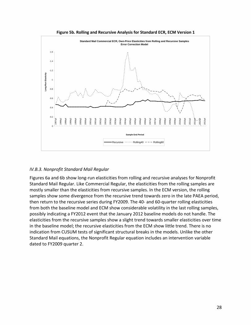
28

Figure 5b. Rolling and Recursive Analysis for Standard ECR, ECM Version 1

IV.B.3. Nonprofit Standard Mail Regular

Figures 6a and 6b show long-run elasticities from rolling and recursive analyses for Nonprofit Standard Mail Regular. Like Commercial Regular, the elasticities from the rolling samples are mostly smaller than the elasticities from recursive samples. In the ECM version, the rolling samples show some divergence from the recursive trend towards zero in the late PAEA period, then return to the recursive series during FY2009. The 40- and 60-quarter rolling elasticities from both the baseline model and ECM show considerable volatility in the last rolling samples, possibly indicating a FY2012 event that the January 2012 baseline models do not handle. The elasticities from the recursive samples show a slight trend towards smaller elasticities over time in the baseline model; the recursive elasticities from the ECM show little trend. There is no indication from CUSUM tests of significant structural breaks in the models. Unlike the other Standard Mail equations, the Nonprofit Regular equation includes an intervention variable dated to FY2009 quarter 2.

Standard Mail Commercial ECR, Own-Price Elasticities from Rolling and Recursive SamplesError Correction Model

-1.6

-1.4

-1.2

-1

-0.8

-0.6

-0.4

-0.2

0

1997

q4

1998

q2

1998

q4

1999

q2

1999

q4

2000

q2

2000

q4

2001

q2

2001

q4

2002

q2

2002

q4

2003

q2

2003

q4

2004

q2

2004

q4

2005

q2

2005

q4

2006

q2

2006

q4

2007

q2

2007

q4

2008

q2

2008

q4

2009

q2

2009

q4

2010

q2

2010

q4

2011

q2

2011

q4

2012

q2

2012

q4

Sample End Period

Long

-Run

Ela

stic

ity

Recursive Rolling40 Rolling60

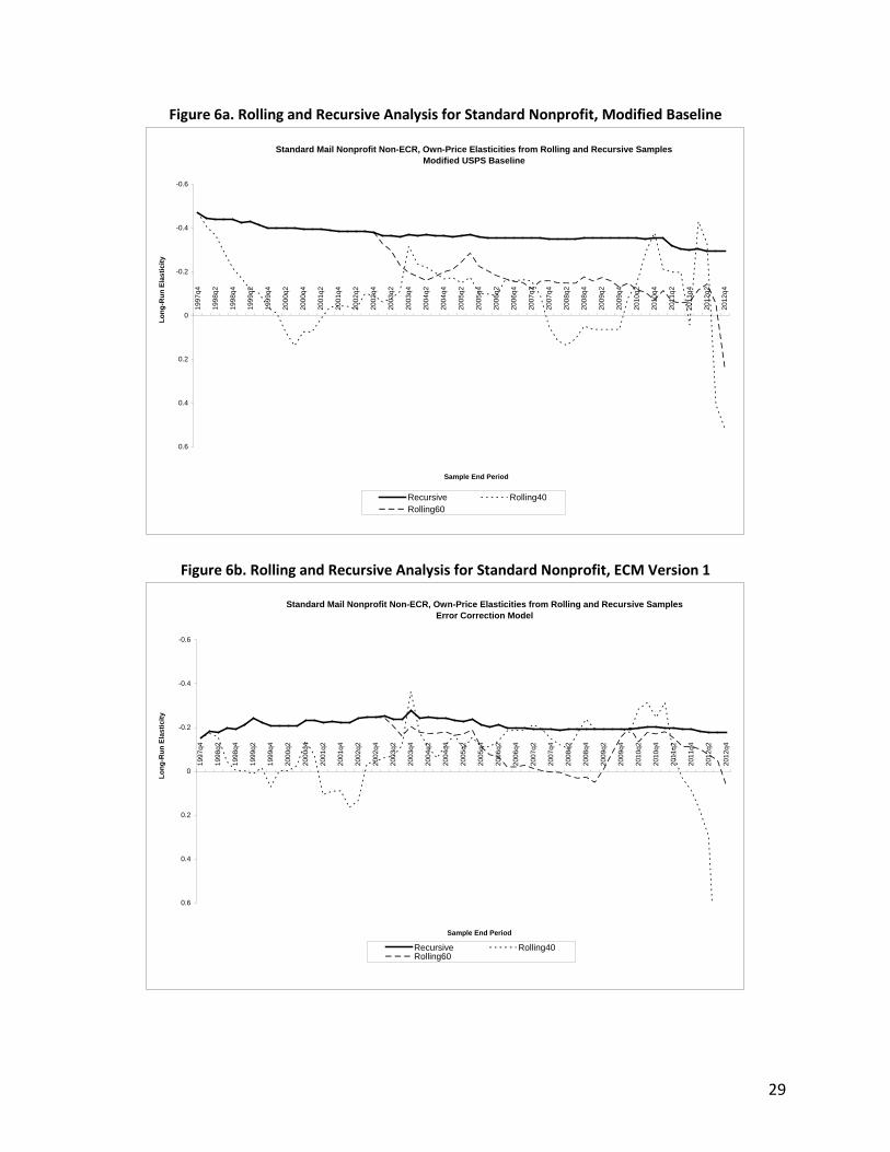
29

Figure 6a. Rolling and Recursive Analysis for Standard Nonprofit, Modified Baseline

Figure 6b. Rolling and Recursive Analysis for Standard Nonprofit, ECM Version 1

Standard Mail Nonprofit Non-ECR, Own-Price Elasticities from Rolling and Recursive SamplesModified USPS Baseline

-0.6

-0.4

-0.2

0

0.2

0.4

0.6

1997

q4

1998

q2

1998

q4

1999

q2

1999

q4

2000

q2

2000

q4

2001

q2

2001

q4

2002

q2

2002

q4

2003

q2

2003

q4

2004

q2

2004

q4

2005

q2

2005

q4

2006

q2

2006

q4

2007

q2

2007

q4

2008

q2

2008

q4

2009

q2

2009

q4

2010

q2

2010

q4

2011

q2

2011

q4

2012

q2

2012

q4

Sample End Period

Long

-Run

Ela

stic

ity

Recursive Rolling40Rolling60

Standard Mail Nonprofit Non-ECR, Own-Price Elasticities from Rolling and Recursive SamplesError Correction Model

-0.6

-0.4

-0.2

0

0.2

0.4

0.6

1997

q4

1998

q2

1998

q4

1999

q2

1999

q4

2000

q2

2000

q4

2001

q2

2001

q4

2002

q2

2002

q4

2003

q2

2003

q4

2004

q2

2004

q4

2005

q2

2005

q4

2006

q2

2006

q4

2007

q2

2007

q4

2008

q2

2008

q4

2009

q2

2009

q4

2010

q2

2010

q4

2011

q2

2011

q4

2012

q2

2012

q4

Sample End Period

Long

-Run

Ela

stic

ity

Recursive Rolling40Rolling60

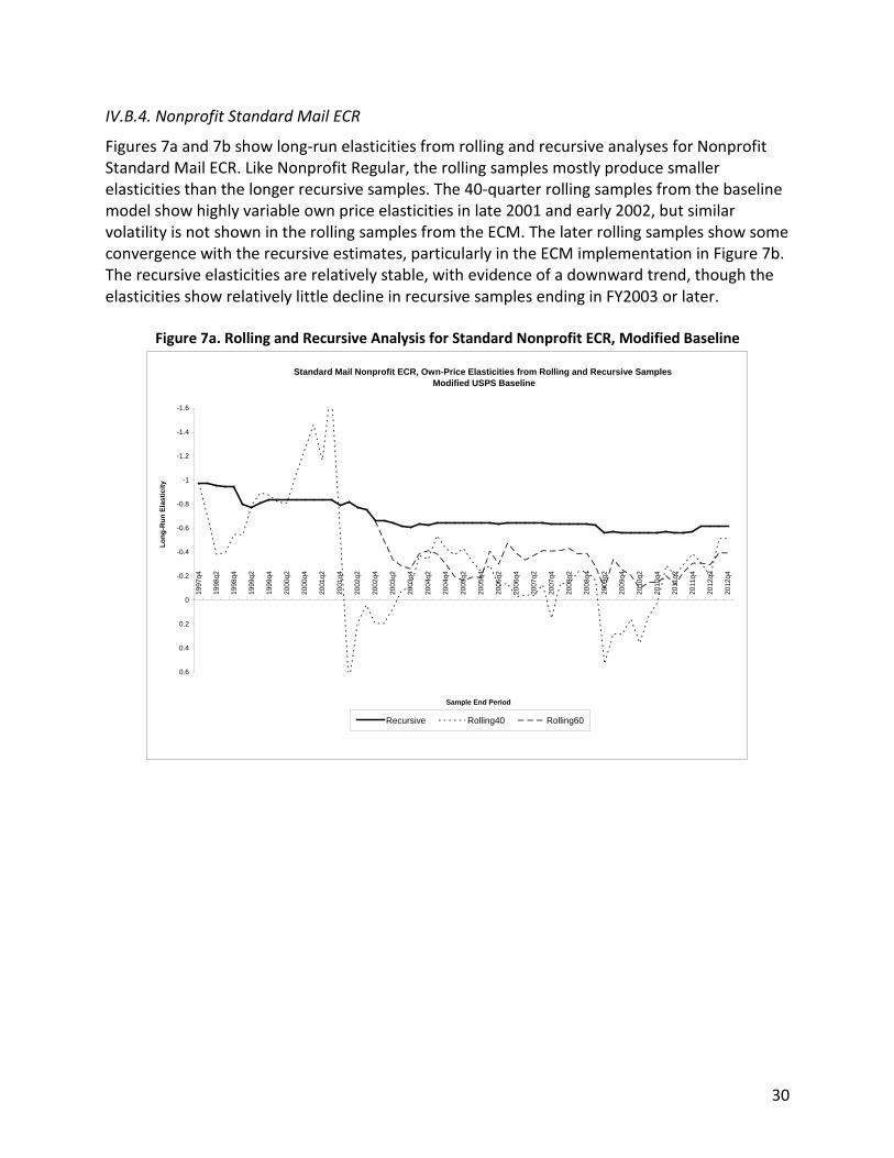
30

IV.B.4. Nonprofit Standard Mail ECR

Figures 7a and 7b show long-run elasticities from rolling and recursive analyses for Nonprofit Standard Mail ECR. Like Nonprofit Regular, the rolling samples mostly produce smaller elasticities than the longer recursive samples. The 40-quarter rolling samples from the baseline model show highly variable own price elasticities in late 2001 and early 2002, but similar volatility is not shown in the rolling samples from the ECM. The later rolling samples show some convergence with the recursive estimates, particularly in the ECM implementation in Figure 7b. The recursive elasticities are relatively stable, with evidence of a downward trend, though the elasticities show relatively little decline in recursive samples ending in FY2003 or later.

Figure 7a. Rolling and Recursive Analysis for Standard Nonprofit ECR, Modified Baseline

Standard Mail Nonprofit ECR, Own-Price Elasticities from Rolling and Recursive Samples Modified USPS Baseline

-1.6

-1.4

-1.2

-1

-0.8

-0.6

-0.4

-0.2

0

0.2

0.4

0.6

1997

q4

1998

q2

1998

q4

1999

q2

1999

q4

2000

q2

2000

q4

2001

q2

2001

q4

2002

q2

2002

q4

2003

q2

2003

q4

2004

q2

2004

q4

2005

q2

2005

q4

2006

q2

2006

q4

2007

q2

2007

q4

2008

q2

2008

q4

2009

q2

2009

q4

2010

q2

2010

q4

2011

q2

2011

q4

2012

q2

2012

q4

Sample End Period

Long

-Run

Ela

stic

ity

Recursive Rolling40 Rolling60

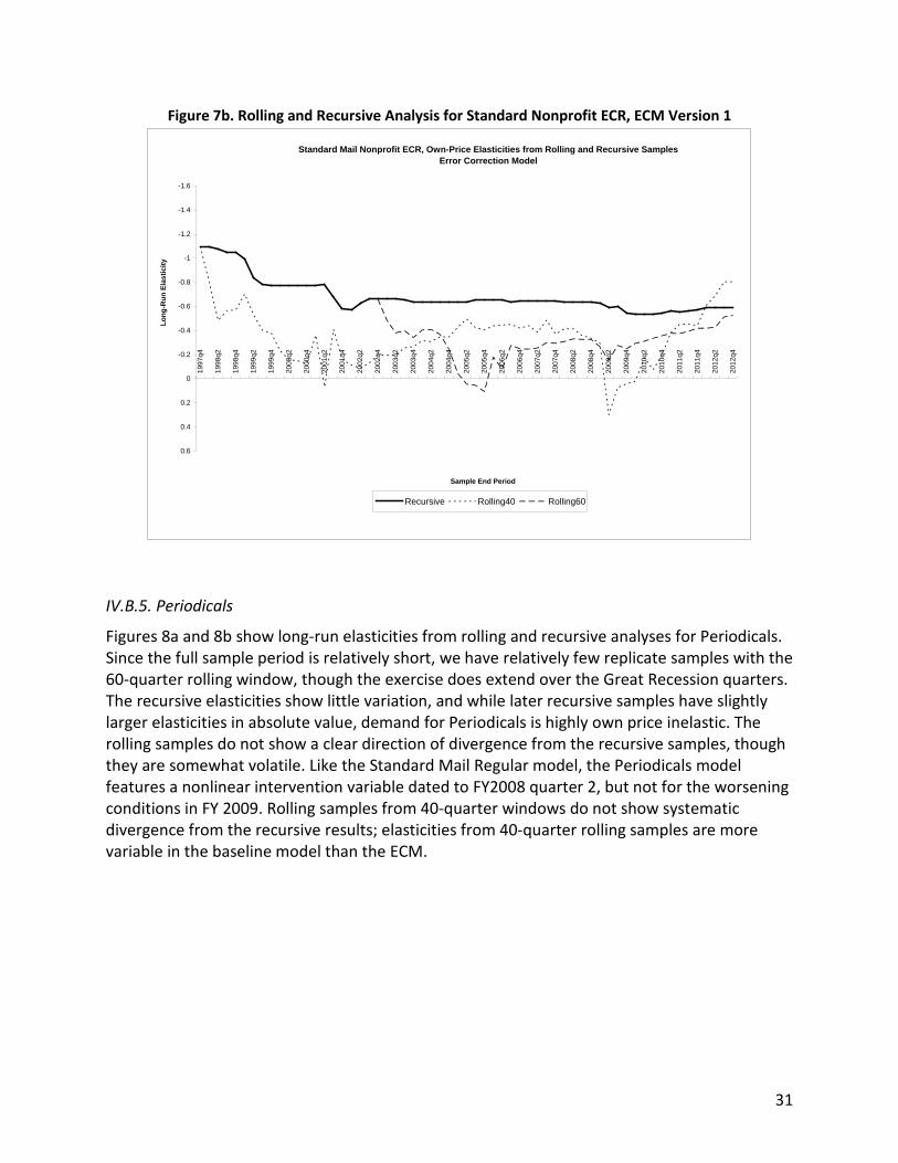
31

Figure 7b. Rolling and Recursive Analysis for Standard Nonprofit ECR, ECM Version 1

IV.B.5. Periodicals

Figures 8a and 8b show long-run elasticities from rolling and recursive analyses for Periodicals. Since the full sample period is relatively short, we have relatively few replicate samples with the 60-quarter rolling window, though the exercise does extend over the Great Recession quarters. The recursive elasticities show little variation, and while later recursive samples have slightly larger elasticities in absolute value, demand for Periodicals is highly own price inelastic. The rolling samples do not show a clear direction of divergence from the recursive samples, though they are somewhat volatile. Like the Standard Mail Regular model, the Periodicals model features a nonlinear intervention variable dated to FY2008 quarter 2, but not for the worsening conditions in FY 2009. Rolling samples from 40-quarter windows do not show systematic divergence from the recursive results; elasticities from 40-quarter rolling samples are more variable in the baseline model than the ECM.

Standard Mail Nonprofit ECR, Own-Price Elasticities from Rolling and Recursive SamplesError Correction Model

-1.6

-1.4

-1.2

-1

-0.8

-0.6

-0.4

-0.2

0

0.2

0.4

0.6

1997

q4

1998

q2

1998

q4

1999

q2

1999

q4

2000

q2

2000

q4

2001

q2

2001

q4

2002

q2

2002

q4

2003

q2

2003

q4

2004

q2

2004

q4

2005

q2

2005

q4

2006

q2

2006

q4

2007

q2

2007

q4

2008

q2

2008

q4

2009

q2

2009

q4

2010

q2

2010

q4

2011

q2

2011

q4

2012

q2

2012

q4

Sample End Period

Long

-Run

Ela

stic

ity

Recursive Rolling40 Rolling60

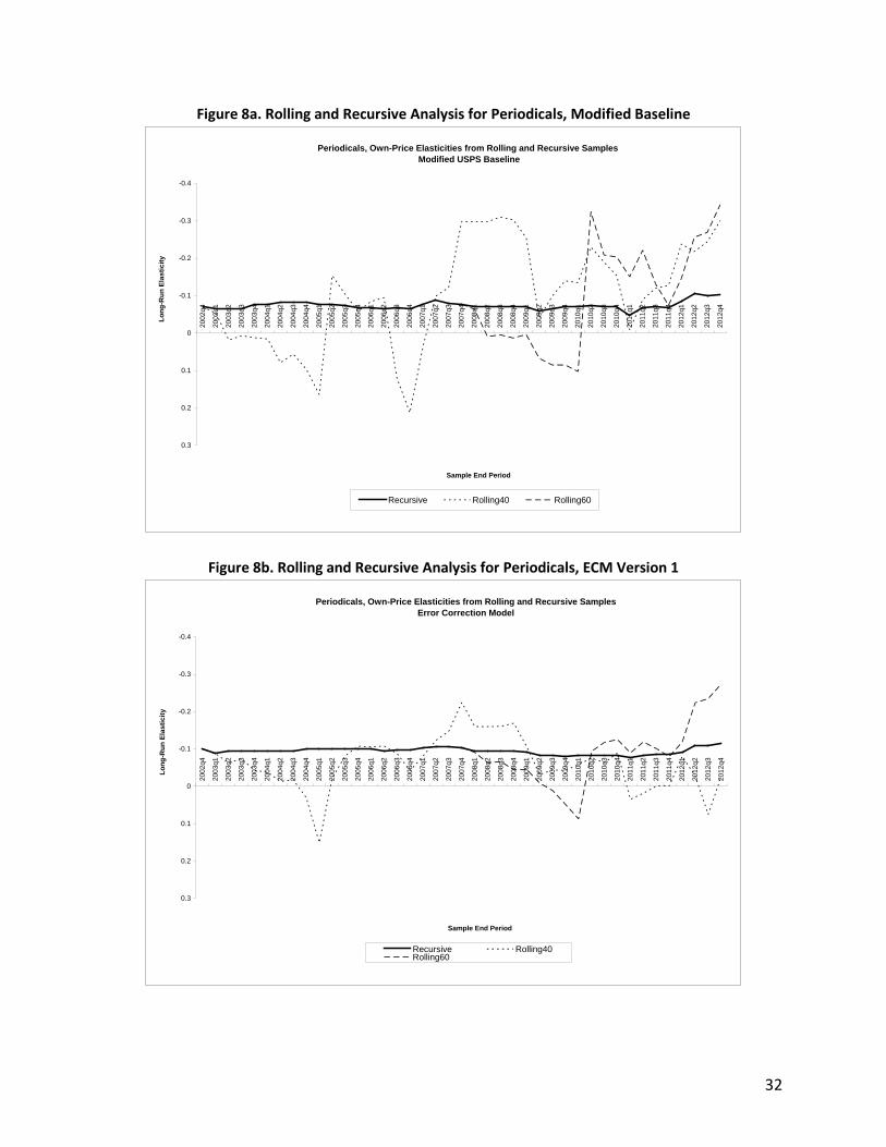
32

Figure 8a. Rolling and Recursive Analysis for Periodicals, Modified Baseline

Figure 8b. Rolling and Recursive Analysis for Periodicals, ECM Version 1

Periodicals, Own-Price Elasticities from Rolling and Recursive Samples Modified USPS Baseline

-0.4

-0.3

-0.2

-0.1

0

0.1

0.2

0.3

2002

q4

2003

q1

2003

q2

2003

q3

2003

q4

2004

q1

2004

q2

2004

q3

2004

q4

2005

q1

2005

q2

2005

q3

2005

q4

2006

q1

2006

q2

2006

q3

2006

q4

2007

q1

2007

q2

2007

q3

2007

q4

2008

q1

2008

q2

2008

q3

2008

q4

2009

q1

2009

q2

2009

q3

2009

q4

2010

q1

2010

q2

2010

q3

2010

q4

2011

q1

2011

q2

2011

q3

2011

q4

2012

q1

2012

q2

2012

q3

2012

q4

Sample End Period

Long

-Run

Ela

stic

ity

Recursive Rolling40 Rolling60

Periodicals, Own-Price Elasticities from Rolling and Recursive SamplesError Correction Model

-0.4

-0.3

-0.2

-0.1

0

0.1

0.2

0.3

2002

q4

2003

q1

2003

q2

2003

q3

2003

q4

2004

q1

2004

q2

2004

q3

2004

q4

2005

q1

2005

q2

2005

q3

2005

q4

2006

q1

2006

q2

2006

q3

2006

q4

2007

q1

2007

q2

2007

q3

2007

q4

2008

q1

2008

q2

2008

q3

2008

q4

2009

q1

2009

q2

2009

q3

2009

q4

2010

q1

2010

q2

2010

q3

2010

q4

2011

q1

2011

q2

2011

q3

2011

q4

2012

q1

2012

q2

2012

q3

2012

q4

Sample End Period

Long

-Run

Ela

stic

ity

Recursive Rolling40Rolling60

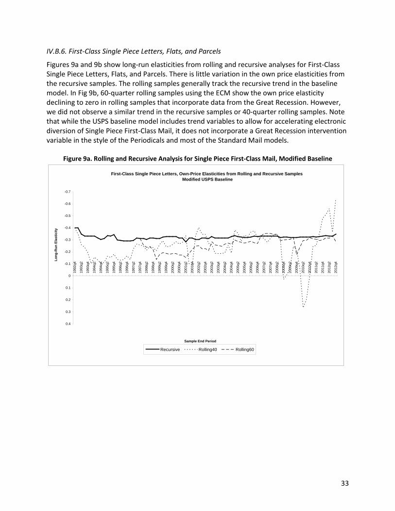
33

IV.B.6. First-Class Single Piece Letters, Flats, and Parcels

Figures 9a and 9b show long-run elasticities from rolling and recursive analyses for First-Class Single Piece Letters, Flats, and Parcels. There is little variation in the own price elasticities from the recursive samples. The rolling samples generally track the recursive trend in the baseline model. In Fig 9b, 60-quarter rolling samples using the ECM show the own price elasticity declining to zero in rolling samples that incorporate data from the Great Recession. However, we did not observe a similar trend in the recursive samples or 40-quarter rolling samples. Note that while the USPS baseline model includes trend variables to allow for accelerating electronic diversion of Single Piece First-Class Mail, it does not incorporate a Great Recession intervention variable in the style of the Periodicals and most of the Standard Mail models.

Figure 9a. Rolling and Recursive Analysis for Single Piece First-Class Mail, Modified Baseline

First-Class Single Piece Letters, Own-Price Elasticities from Rolling and Recursive Samples Modified USPS Baseline

-0.7

-0.6

-0.5

-0.4

-0.3

-0.2

-0.1

0

0.1

0.2

0.3

0.4

1992

q4

1993

q2

1993

q4

1994

q2

1994

q4

1995

q2

1995

q4

1996

q2

1996

q4

1997

q2

1997

q4

1998

q2

1998

q4

1999

q2

1999

q4

2000

q2

2000

q4

2001

q2

2001

q4

2002

q2

2002

q4

2003

q2

2003

q4

2004

q2

2004

q4

2005

q2

2005

q4

2006

q2

2006

q4

2007

q2

2007

q4

2008

q2

2008

q4

2009

q2

2009

q4

2010

q2

2010

q4

2011

q2

2011

q4

2012

q2

2012

q4

Sample End Period

Long

-Run

Ela

stic

ity

Recursive Rolling40 Rolling60

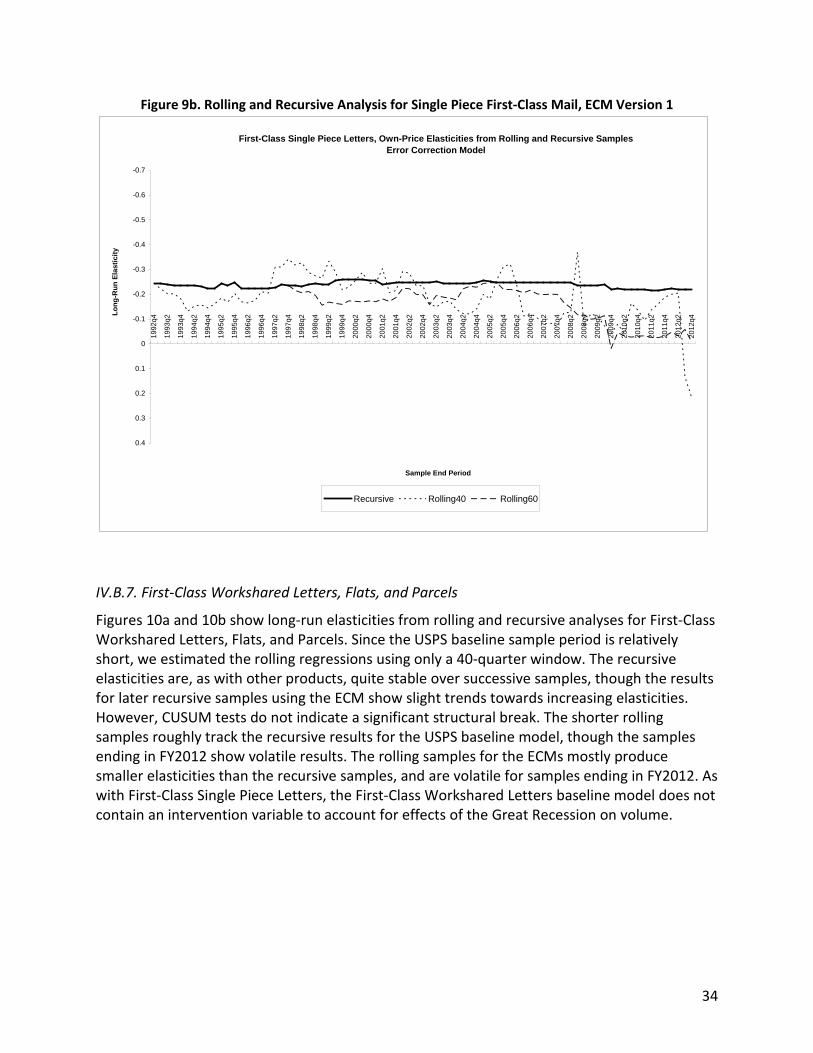
34

Figure 9b. Rolling and Recursive Analysis for Single Piece First-Class Mail, ECM Version 1

IV.B.7. First-Class Workshared Letters, Flats, and Parcels

Figures 10a and 10b show long-run elasticities from rolling and recursive analyses for First-Class Workshared Letters, Flats, and Parcels. Since the USPS baseline sample period is relatively short, we estimated the rolling regressions using only a 40-quarter window. The recursive elasticities are, as with other products, quite stable over successive samples, though the results for later recursive samples using the ECM show slight trends towards increasing elasticities. However, CUSUM tests do not indicate a significant structural break. The shorter rolling samples roughly track the recursive results for the USPS baseline model, though the samples ending in FY2012 show volatile results. The rolling samples for the ECMs mostly produce smaller elasticities than the recursive samples, and are volatile for samples ending in FY2012. As with First-Class Single Piece Letters, the First-Class Workshared Letters baseline model does not contain an intervention variable to account for effects of the Great Recession on volume.

First-Class Single Piece Letters, Own-Price Elasticities from Rolling and Recursive SamplesError Correction Model

-0.7

-0.6

-0.5

-0.4

-0.3

-0.2

-0.1

0

0.1

0.2

0.3

0.4

1992

q4

1993

q2

1993

q4

1994

q2

1994

q4

1995

q2

1995

q4

1996

q2

1996

q4

1997

q2

1997

q4

1998

q2

1998

q4

1999

q2

1999

q4

2000

q2

2000

q4

2001

q2

2001

q4

2002

q2

2002

q4

2003

q2

2003

q4

2004

q2

2004

q4

2005

q2

2005

q4

2006

q2

2006

q4

2007

q2

2007

q4

2008

q2

2008

q4

2009

q2

2009

q4

2010

q2

2010

q4

2011

q2

2011

q4

2012

q2

2012

q4

Sample End Period

Long

-Run

Ela

stic

ity

Recursive Rolling40 Rolling60

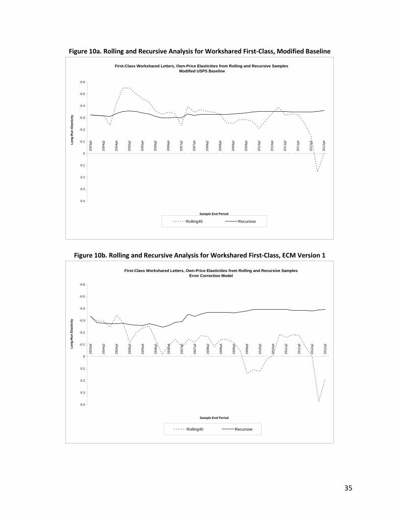
35

Figure 10a. Rolling and Recursive Analysis for Workshared First-Class, Modified Baseline

Figure 10b. Rolling and Recursive Analysis for Workshared First-Class, ECM Version 1

First-Class Workshared Letters, Own-Price Elasticities from Rolling and Recursive Samples Modified USPS Baseline

-0.6

-0.5

-0.4

-0.3

-0.2

-0.1

0

0.1

0.2

0.3

0.4

2003

q4

2004

q2

2004

q4

2005

q2

2005

q4

2006

q2

2006

q4

2007

q2

2007

q4

2008

q2

2008

q4

2009

q2

2009

q4

2010

q2

2010

q4

2011

q2

2011

q4

2012

q2

2012

q4

Sample End Period

Long

-Run

Ela

stic

ity

Rolling40 Recursive

First-Class Workshared Letters, Own-Price Elasticities from Rolling and Recursive SamplesError Correction Model

-0.6

-0.5

-0.4

-0.3

-0.2

-0.1

0

0.1

0.2

0.3

0.4

2003

q4

2004

q2

2004

q4

2005

q2

2005

q4

2006

q2

2006

q4

2007

q2

2007

q4

2008

q2

2008

q4

2009

q2

2009

q4

2010

q2

2010

q4

2011

q2

2011

q4

2012

q2

2012

q4

Sample End Period

Long

-Run

Ela

stic

ity

Rolling40 Recursive

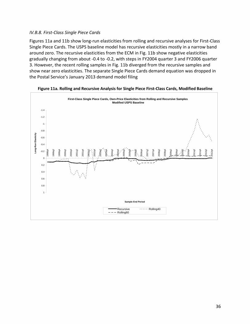
36

IV.B.8. First-Class Single Piece Cards

Figures 11a and 11b show long-run elasticities from rolling and recursive analyses for First-Class Single Piece Cards. The USPS baseline model has recursive elasticities mostly in a narrow band around zero. The recursive elasticities from the ECM in Fig. 11b show negative elasticities gradually changing from about -0.4 to -0.2, with steps in FY2004 quarter 3 and FY2006 quarter 3. However, the recent rolling samples in Fig. 11b diverged from the recursive samples and show near zero elasticities. The separate Single Piece Cards demand equation was dropped in the Postal Service’s January 2013 demand model filing

Figure 11a. Rolling and Recursive Analysis for Single Piece First-Class Cards, Modified Baseline

First-Class Single Piece Cards, Own-Price Elasticities from Rolling and Recursive Samples Modified USPS Baseline

-1.4

-1.2

-1

-0.8

-0.6

-0.4

-0.2

0

0.2

0.4

0.6

0.8

1

1998

q4

1999

q2

1999

q4

2000

q2

2000

q4

2001

q2

2001

q4

2002

q2

2002

q4

2003

q2

2003

q4

2004

q2

2004

q4

2005

q2

2005

q4

2006

q2

2006

q4

2007

q2

2007

q4

2008

q2

2008

q4

2009

q2

2009

q4

2010

q2

2010

q4

2011

q2

2011

q4

2012

q2

2012

q4

Sample End Period

Long

-Run

Ela

stic

ity

Recursive Rolling40Rolling60

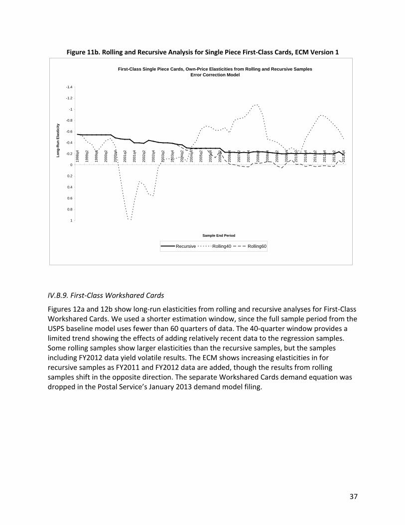
37

Figure 11b. Rolling and Recursive Analysis for Single Piece First-Class Cards, ECM Version 1

IV.B.9. First-Class Workshared Cards

Figures 12a and 12b show long-run elasticities from rolling and recursive analyses for First-Class Workshared Cards. We used a shorter estimation window, since the full sample period from the USPS baseline model uses fewer than 60 quarters of data. The 40-quarter window provides a limited trend showing the effects of adding relatively recent data to the regression samples. Some rolling samples show larger elasticities than the recursive samples, but the samples including FY2012 data yield volatile results. The ECM shows increasing elasticities in for recursive samples as FY2011 and FY2012 data are added, though the results from rolling samples shift in the opposite direction. The separate Workshared Cards demand equation was dropped in the Postal Service’s January 2013 demand model filing.

First-Class Single Piece Cards, Own-Price Elasticities from Rolling and Recursive SamplesError Correction Model

-1.4

-1.2

-1

-0.8

-0.6

-0.4

-0.2

0

0.2

0.4

0.6

0.8

1

1998

q4

1999

q2

1999

q4

2000

q2

2000

q4

2001

q2

2001

q4

2002

q2

2002

q4

2003

q2

2003

q4

2004

q2

2004

q4

2005

q2

2005

q4

2006

q2

2006

q4

2007

q2

2007

q4

2008

q2

2008

q4

2009

q2

2009

q4

2010

q2

2010

q4

2011

q2

2011

q4

2012

q2

2012

q4

Sample End Period

Long

-Run

Ela

stic

ity

Recursive Rolling40 Rolling60

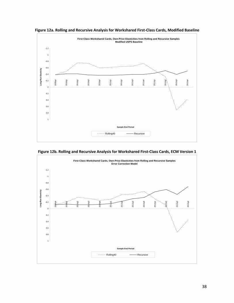
38

Figure 12a. Rolling and Recursive Analysis for Workshared First-Class Cards, Modified Baseline

Figure 12b. Rolling and Recursive Analysis for Workshared First-Class Cards, ECM Version 1

First-Class Workshared Cards, Own-Price Elasticities from Rolling and Recursive Samples Modified USPS Baseline

-1.2

-1

-0.8

-0.6

-0.4

-0.2

0

0.2

0.4

0.6

0.8

1

2009

q4

2010

q1

2010

q2

2010

q3

2010

q4

2011

q1

2011

q2

2011

q3

2011

q4

2012

q1

2012

q2

2012

q3

2012

q4

Sample End Period

Long

-Run

Ela

stic

ity

Rolling40 Recursive

First-Class Workshared Cards, Own-Price Elasticities from Rolling and Recursive SamplesError Correction Model

-1.2

-1

-0.8

-0.6

-0.4

-0.2

0

0.2

0.4

0.6

0.8

1

2009

q4

2010

q1

2010

q2

2010

q3

2010

q4

2011

q1

2011

q2

2011

q3

2011

q4

2012

q1

2012

q2

2012

q3

2012

q4

Sample End Period

Long

-Run

Ela

stic

ity

Rolling40 Recursive

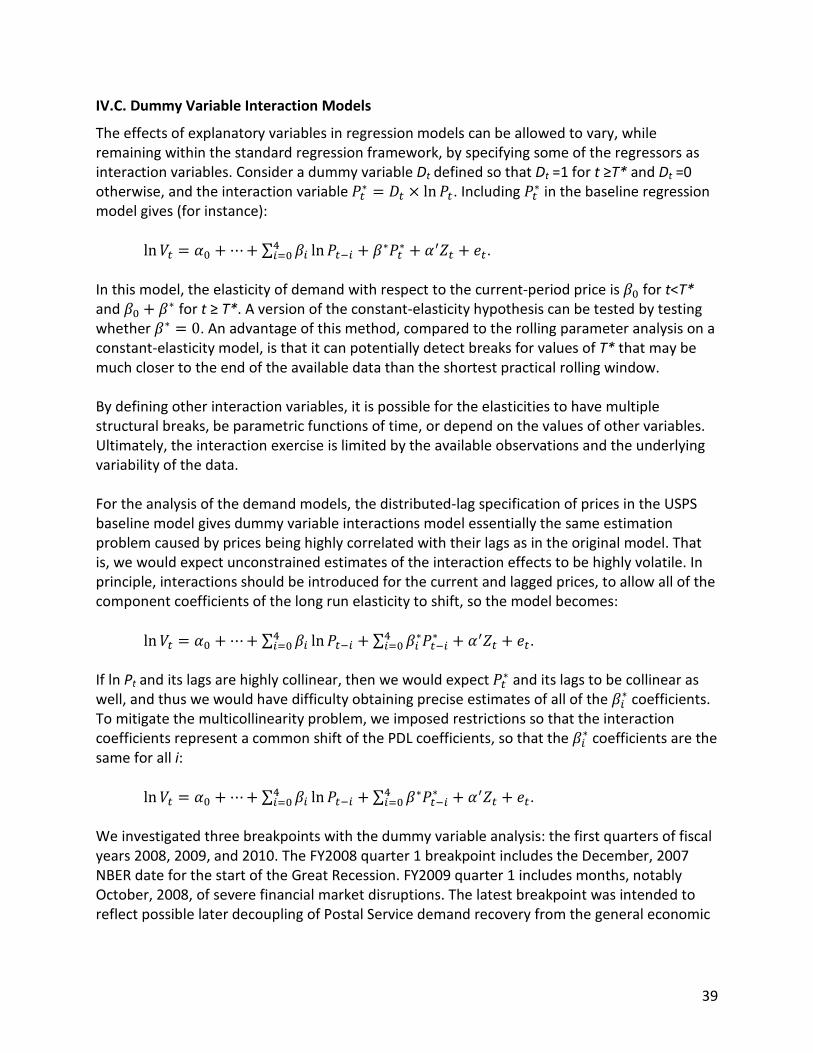
39

IV.C. Dummy Variable Interaction Models

The effects of explanatory variables in regression models can be allowed to vary, while remaining within the standard regression framework, by specifying some of the regressors as interaction variables. Consider a dummy variable Dt defined so that Dt =1 for t ≥T* and Dt =0 otherwise, and the interaction variable 𝑃𝑡∗ = 𝐷𝑡 × ln𝑃𝑡. Including 𝑃𝑡∗ in the baseline regression model gives (for instance): ln𝑉𝑡 = 𝛼0 + ⋯+ ∑ 𝛽𝑖 ln𝑃𝑡−𝑖4

𝑖=0 + 𝛽∗𝑃𝑡∗ + 𝛼′𝑍𝑡 + 𝑒𝑡. In this model, the elasticity of demand with respect to the current-period price is 𝛽0 for t<T* and 𝛽0 + 𝛽∗ for t ≥ T*. A version of the constant-elasticity hypothesis can be tested by testing whether 𝛽∗ = 0. An advantage of this method, compared to the rolling parameter analysis on a constant-elasticity model, is that it can potentially detect breaks for values of T* that may be much closer to the end of the available data than the shortest practical rolling window. By defining other interaction variables, it is possible for the elasticities to have multiple structural breaks, be parametric functions of time, or depend on the values of other variables. Ultimately, the interaction exercise is limited by the available observations and the underlying variability of the data. For the analysis of the demand models, the distributed-lag specification of prices in the USPS baseline model gives dummy variable interactions model essentially the same estimation problem caused by prices being highly correlated with their lags as in the original model. That is, we would expect unconstrained estimates of the interaction effects to be highly volatile. In principle, interactions should be introduced for the current and lagged prices, to allow all of the component coefficients of the long run elasticity to shift, so the model becomes: ln𝑉𝑡 = 𝛼0 + ⋯+ ∑ 𝛽𝑖 ln𝑃𝑡−𝑖4

𝑖=0 + ∑ 𝛽𝑖∗𝑃𝑡−𝑖∗4𝑖=0 + 𝛼′𝑍𝑡 + 𝑒𝑡.

If ln Pt and its lags are highly collinear, then we would expect 𝑃𝑡∗ and its lags to be collinear as well, and thus we would have difficulty obtaining precise estimates of all of the 𝛽𝑖∗ coefficients. To mitigate the multicollinearity problem, we imposed restrictions so that the interaction coefficients represent a common shift of the PDL coefficients, so that the 𝛽𝑖∗ coefficients are the same for all i: ln𝑉𝑡 = 𝛼0 + ⋯+ ∑ 𝛽𝑖 ln𝑃𝑡−𝑖4

𝑖=0 + ∑ 𝛽∗𝑃𝑡−𝑖∗4𝑖=0 + 𝛼′𝑍𝑡 + 𝑒𝑡.

We investigated three breakpoints with the dummy variable analysis: the first quarters of fiscal years 2008, 2009, and 2010. The FY2008 quarter 1 breakpoint includes the December, 2007 NBER date for the start of the Great Recession. FY2009 quarter 1 includes months, notably October, 2008, of severe financial market disruptions. The latest breakpoint was intended to reflect possible later decoupling of Postal Service demand recovery from the general economic

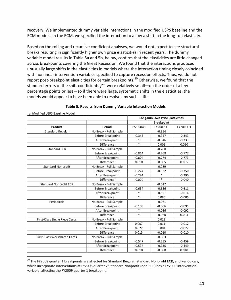
40

recovery. We implemented dummy variable interactions in the modified USPS baseline and the ECM models. In the ECM, we specified the interaction to allow a shift in the long-run elasticity. Based on the rolling and recursive coefficient analyses, we would not expect to see structural breaks resulting in significantly higher own price elasticities in recent years. The dummy variable model results in Table 5a and 5b, below, confirm that the elasticities are little changed across breakpoints covering the Great Recession. We found that the interactions produced unusually large shifts in the elasticities in models where the interaction timing closely coincided with nonlinear intervention variables specified to capture recession effects. Thus, we do not report post-breakpoint elasticities for certain breakpoints.30 Otherwise, we found that the standard errors of the shift coefficients 𝛽∗ were relatively small—on the order of a few percentage points or less—so if there were large, systematic shifts in the elasticities, the models would appear to have been able to resolve any such shifts.

Table 5. Results from Dummy Variable Interaction Models

a. Modified USPS Baseline Model Long-Run Own Price Elasticities Breakpoint

Product Period FY2008Q1 FY2009Q1 FY2010Q1 Standard Regular No Break - Full Sample -0.354

Before Breakpoint -0.343 -0.347 -0.343 After Breakpoint * -0.346 -0.333 Difference * 0.001 0.010

Standard ECR No Break - Full Sample -0.780 Before Breakpoint -0.814 -0.768 -0.777 After Breakpoint -0.804 -0.774 -0.773 Difference 0.010 -0.005 0.005

Standard Nonprofit No Break - Full Sample -0.289 Before Breakpoint -0.274 -0.322 -0.350 After Breakpoint -0.294 * -0.390 Difference -0.020 * -0.040

Standard Nonprofit ECR No Break - Full Sample -0.617 Before Breakpoint -0.634 -0.636 -0.611 After Breakpoint * -0.551 -0.616 Difference * 0.085 -0.005

Periodicals No Break - Full Sample -0.071 Before Breakpoint -0.103 -0.066 -0.095 After Breakpoint * -0.086 -0.092 Difference * -0.020 0.004

First-Class Single Piece Cards No Break - Full Sample 0.013 Before Breakpoint 0.007 0.011 -0.012 After Breakpoint 0.022 0.001 -0.022 Difference 0.015 -0.010 -0.010

First-Class Workshared Cards No Break - Full Sample -0.383 Before Breakpoint -0.547 -0.255 -0.459 After Breakpoint -0.537 -0.335 -0.449 Difference 0.010 -0.080 0.010

30 The FY2008 quarter 1 breakpoints are affected for Standard Regular, Standard Nonprofit ECR, and Periodicals, which incorporate interventions at FY2008 quarter 2; Standard Nonprofit (non-ECR) has a FY2009 intervention variable, affecting the FY2009 quarter 1 breakpoint.

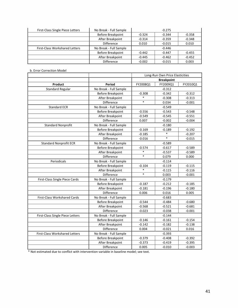
41

First-Class Single Piece Letters No Break - Full Sample -0.275 Before Breakpoint -0.324 -0.344 -0.358 After Breakpoint -0.314 -0.359 -0.348 Difference 0.010 -0.015 0.010

First-Class Workshared Letters No Break - Full Sample -0.446 Before Breakpoint -0.442 -0.447 -0.455 After Breakpoint -0.445 -0.462 -0.452

Difference -0.002 -0.015 0.003

b. Error Correction Model Long-Run Own Price Elasticities Breakpoint

Product Period FY2008Q1 FY2009Q1 FY2010Q1 Standard Regular No Break - Full Sample -0.312

Before Breakpoint -0.308 -0.342 -0.312 After Breakpoint * -0.308 -0.313 Difference * 0.034 -0.001

Standard ECR No Break - Full Sample -0.549 Before Breakpoint -0.556 -0.543 -0.548 After Breakpoint -0.549 -0.545 -0.551 Difference 0.007 -0.002 -0.004

Standard Nonprofit No Break - Full Sample -0.180 Before Breakpoint -0.169 -0.189 -0.192 After Breakpoint -0.185 * -0.207 Difference -0.016 * -0.015

Standard Nonprofit ECR No Break - Full Sample -0.589 Before Breakpoint -0.574 -0.617 -0.589 After Breakpoint * -0.537 -0.589 Difference * 0.079 0.000

Periodicals No Break - Full Sample -0.114 Before Breakpoint -0.104 -0.119 -0.115 After Breakpoint * -0.115 -0.116 Difference * 0.003 -0.001

First-Class Single Piece Cards No Break - Full Sample -0.179 Before Breakpoint -0.187 -0.212 -0.185 After Breakpoint -0.181 -0.196 -0.180 Difference 0.006 0.016 0.005

First-Class Workshared Cards No Break - Full Sample -0.683 Before Breakpoint -0.544 -0.484 -0.680 After Breakpoint -0.568 -0.521 -0.681 Difference -0.023 -0.038 -0.001

First-Class Single Piece Letters No Break - Full Sample -0.144 Before Breakpoint -0.146 -0.161 -0.154 After Breakpoint -0.142 -0.182 -0.138 Difference 0.004 -0.021 0.016

First-Class Workshared Letters No Break - Full Sample -0.393 Before Breakpoint -0.379 -0.408 -0.392 After Breakpoint -0.373 -0.419 -0.395

Difference 0.005 -0.010 -0.003 * Not estimated due to conflict with intervention variable in baseline model; see text.

42

V. CONCLUSIONS

The significant volume losses of recent years have, understandably, led observers to consider a broad range of potential factors that may account for the declines, including increasing price sensitivity of mailers. Real U.S. postal rates have shown very little variation in recent years, and cannot themselves be a major factor of volume losses, compared to modal competition and recessionary drops in economic activity drivers. Nevertheless, it is possible that U.S. demands for postal services could have become more own price elastic with significant implications for pricing policies. The relatively long time periods needed for the estimation samples of the demand models, combined with constant elasticity assumptions in the log-linear demand equations, could in theory have attenuated changes in the own price elasticities. We tested the stability of the Postal Service’s demand models for market dominant products both by varying the regression sample periods and by investigating whether there is evidence for recent structural breaks in the elasticity estimates. We found some technical deficiencies in the Postal Service’s baseline models related to time series properties of the volume and economic activity variables, and possibly also the price indexes. We recommend that the Postal Service’s analysts address these issues in future demand model updates. We find no evidence that the Postal Service’s demand models are systematically understating own price elasticities of demand for the market dominant products we studied. Indeed, to the extent the analysis shows own price elasticities to be “in flux,” the changes are predominantly in the direction of lower own price elasticities. Additionally, the data do not suggest that the inclusion of older observations in the demand regressions result in smaller elasticity estimates. The overall picture is that while demands for market dominant postal products have shifted substantially due to a combination of factors other than postal prices, they remain own price inelastic.

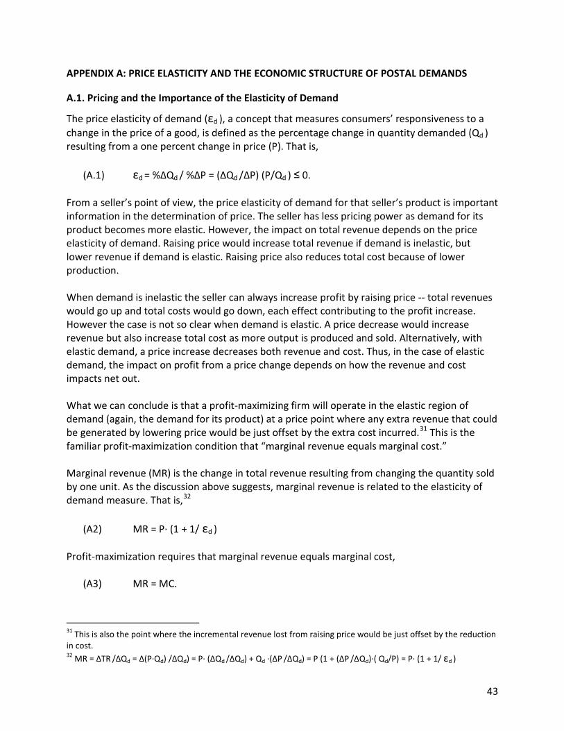
43

APPENDIX A: PRICE ELASTICITY AND THE ECONOMIC STRUCTURE OF POSTAL DEMANDS

A.1. Pricing and the Importance of the Elasticity of Demand

The price elasticity of demand (εd ), a concept that measures consumers’ responsiveness to a change in the price of a good, is defined as the percentage change in quantity demanded (Qd ) resulting from a one percent change in price (P). That is,

(A.1) εd = %∆Qd / %∆P = (∆Qd /∆P) (P/Qd ) ≤ 0.

From a seller’s point of view, the price elasticity of demand for that seller’s product is important information in the determination of price. The seller has less pricing power as demand for its product becomes more elastic. However, the impact on total revenue depends on the price elasticity of demand. Raising price would increase total revenue if demand is inelastic, but lower revenue if demand is elastic. Raising price also reduces total cost because of lower production. When demand is inelastic the seller can always increase profit by raising price -- total revenues would go up and total costs would go down, each effect contributing to the profit increase. However the case is not so clear when demand is elastic. A price decrease would increase revenue but also increase total cost as more output is produced and sold. Alternatively, with elastic demand, a price increase decreases both revenue and cost. Thus, in the case of elastic demand, the impact on profit from a price change depends on how the revenue and cost impacts net out. What we can conclude is that a profit-maximizing firm will operate in the elastic region of demand (again, the demand for its product) at a price point where any extra revenue that could be generated by lowering price would be just offset by the extra cost incurred.31 This is the familiar profit-maximization condition that “marginal revenue equals marginal cost.” Marginal revenue (MR) is the change in total revenue resulting from changing the quantity sold by one unit. As the discussion above suggests, marginal revenue is related to the elasticity of demand measure. That is,32

(A2) MR = P∙ (1 + 1/ εd ) Profit-maximization requires that marginal revenue equals marginal cost,

(A3) MR = MC.

31 This is also the point where the incremental revenue lost from raising price would be just offset by the reduction in cost. 32 MR = ∆TR /∆Qd = ∆(P∙Qd) /∆Qd) = P∙ (∆Qd /∆Qd) + Qd ∙(∆P /∆Qd) = P (1 + (∆P /∆Qd)∙( Qd/P) = P∙ (1 + 1/ εd )

44

Substituting (A3) into (A2) and rearranging gives the profit-maximizing markup equation

(A4) (P – MC) / P = -1/ εd which is also known as the Lerner Index of Market Power.33 This measure shows that a firm’s ability to price above cost is inversely related to the elasticity of demand for its product.34 In the case where marginal cost is a constant, marginal cost and average variable cost are the same and multiplying the left-hand side of (A4) by Q/Q (=1) gives

(A5) Contribution/Revenue ≡ (TR – TVC)/TR = -1/εd. That is, the inverse of the price elasticity of demand for the seller’s product indicates the seller’s ability to generate contribution as a share of revenue (or, equivalently, per unit margin as a share of price). If there is no fixed cost, then total variable cost is total cost and contribution is profit.

For a firm selling multiple products and/or in multiple markets, where the products have independent demands and independent marginal costs,35 (A5) shows that each product’s ability to contribute a share of its revenues toward fixed cost recovery is inversely related to the price elasticity of demand for that product.36 In summary, the price elasticity of demand indicates a firm’s pricing power for a particular product and that product’s ability to generate profit or contribute to fixed cost recovery.

A.2. Determinants of the Price Elasticities of Household Demand

A change in price of a household good or service has two distinct effects on consumer demand. The substitution effect involves using more of a good whose relative price has decreased and less of a good whose relative price has increased. The extent to which substitution is possible is determined by the ability of one good to replace another good in terms of generating consumer satisfaction. When the price of a good increases, other things the same, the relative price of all other goods decrease and the consumer will use less of the good whose price increased and

33 Lerner, A. P. (1934). "The Concept of Monopoly and the Measurement of Monopoly Power". The Review of Economic Studies 1 (3): 157–175. 34 This result has been derived for the single-product profit-maximizing firm. A similar result can be derived for a multi-product not-for-profit firm with fixed costs. Also, closely related is the derivation of Ramsey pricing rules in which second-best efficient fixed cost recovery is achieved through greater price markups in markets with less elastic demand. 35 Independent demands means that the products are neither substitutes nor complements in consumption – the cross-price elasticities of demand are all zero. Independent marginal costs means that the products are neither substitutes nor complements in production – the cross-price elasticities of supply are all zero. 36 The mathematics are more complicated when demands are not independent. In that case, pricing power is inversely related to a “superelasticity of demand” involving the own- and the cross-price elasticities of demand.

45

more of the other goods. Conversely, when the price of a good decreases, consumers will try to substitute it for other goods. The other effect of a price change is the income effect. As the price of a good goes up, the household has less purchasing power for the same budget. Consequently, to remain within its budget constraint a household has to reduce purchases overall. In most cases this means purchasing less of the good. When the price of a good decreases, the household has more purchasing power, and can increase the consumption of some or all goods while remaining on budget. Again, in most cases this means purchasing more of the good.37 We can now identify and discuss some basic determinants of the household’s elasticity of demand for a good.

A.2.a. Substitutes

Demand for a good is more elastic when it is feasible to substitute another good than when it is infeasible. Feasibility of substitution has two conditions. The first condition is technical substitution possibility. That is, can the same satisfaction be generated using the alternative good? The greater the degree of technical substitution of other goods, the more elastic the demand for the good in question. The second condition is availability of the substitute goods. Can the alternative readily be purchased? This condition relates to the price elasticity of supply of the alternative good. The more elastic the supply of a substitute good, the more elastic the demand for the good in question. The demand for a good broadly defined (such as transportation) is less elastic than the demand for a more specific market (such as a particular car make and model). That is because there are few, if any, substitutes for the broadly defined good and more substitutes for the specific good. In the example of transportation goods, the possible substitutes for transportation are limited (walk, bus, taxi, etc.) and imperfect, while there is plethora of close substitutes for a particular model of car from a particular car dealer.

A.2.b. Necessity

The more essential a good is, the less elastic the demand for the good. The necessity of a generic good is reinforced by the absence of feasible substitutes. Historically, postal services have been essential to long distance communication and transport of correspondence. Even though the demand for communication services seems to be always increasing, the development of telephones and subsequent methods of electronic

37 A good is a “normal good” if an increase in incomes results in the consumer purchasing more of that good. A good is an “inferior good” if an increase in income results in the consumer buying less of the good. The income effect reinforces the substitution effect for a normal good and opposes the substitution effect for an inferior good.

46

communications has made postal services per se less essential. Thus, the demand for postal services has been relatively inelastic, but may be becoming more elastic as the essentiality of the services decreases.

A.2.c. Importance in the Household Budget

The larger the share of the household budget allocated to purchase of a good, the more sensitive the consumer is to price. This is because it is worth the effort for the consumer to search out substitution alternatives for these big purchases while it might not be so for purchases that are a very small share of the budget. Also, when the purchases of the good comprise a larger share of the budget, the impact of the income effect from a price change can be substantial. Purchases of postal services have never been a large share of household expenses. Consequently, the demand for these services by households has been relatively inelastic.

A.3.d. Consumer Loyalty and Product Differentiation:

Brand recognition and consumer loyalty to the brand leads to less elastic demand for a good. Advertising by a firm attempts to increase the demand for its product as well as make that demand less elastic. In the postal service context, customer loyalty and product differentiation probably make the demand less elastic for final consumption goods (e.g., a personal letter) but not for intermediate goods which are perceived as commodity inputs.

A.3.e. Time:

Demand is more elastic in the longer run than in the short run. When the price of a good changes, consumers might not be able to immediately search for substitutes and necessity might require keeping purchases largely unchanged. However, with time, the consumer can identify some substitution possibilities that mitigate the impact of a price increase or find additional consumption opportunities in the case of a price decrease. Also, in the very long run, if the price change is viewed as permanent, new products and technologies might be developed.

A.3. Determinants of the Price Elasticities of Business Demand

A change in the price of an input has two distinct impacts on a business’ demand for that input. As with household demand, there is a substitution effect. However, the demand for production inputs by businesses differs from the demand for goods by households because there is no income constraint. Consequently, there is no corresponding income effect as the result of a change in the price of an input. The second effect of a price change on a business’ demand for an input is the scale effect.

47

The substitution effect reflects that the firm can change its mix of inputs to produce a given level of output. As the price of an input increases, the firm, in its effort to minimize cost,38 will substitute other inputs. Conversely, a price decrease for an input will cause the firm to use more of that input and less of other inputs for a given level of production. The extent to which substitution in production can occur is determined by technology. The second impact from a change in the price of an input is the scale effect. The scale effect (also called the expansion effect), takes into account that by changing the firm’s cost (particularly marginal cost), the change in an input price changes the optimal output of the firm. Typically, an increase in the price of an input will shift up (increase) the firm’s marginal cost.39 This results in the profit maximizing output (determined by the equation of marginal revenue and marginal cost) now being less. Conversely, an input price decrease leads to an expansion of output by the firm. If the input price change impacts all firms in the final product industry and the industry is competitive, then the scale effect is enhanced as the industry adjusts to a new equilibrium. That is, an input price increase would result in an initial contraction in output by each firm. However, the increased cost reduces profits and over time leads some firms to exit the industry, further decreasing employment of the input. Conversely, an input price decrease ultimately leads to competitive entry and increasing use of the input. Marshall, in his development of the theory of derived demand, examined the factors on which the elasticity of derived demand depends.40 Marshall identified four conditions, now known as “Marshall’s Rules,” affecting the elasticity of demand for labor. John Hicks undertook a more rigorous mathematical derivation of Marshall’s Rules. 41 Although Marshall and Hicks focused on demand for labor, with the interest being on the effects on the distribution of income among the factors of production in the economy, the analysis is applicable at a more microeconomic level and to any factor of production. Marshall’s Rules (in the order he presented them) are that the demand for an input will be more elastic (1) the greater the ease of technical substitution of other inputs in the production process; (2) the greater the elasticity of demand for final output; (3) the greater the factor’s share of the production cost; and (4) the greater the elasticity of supply of other inputs. Rules (1) and (4) go directly to the substitution effect and are the business demand parallel to the substitution determinant in the household demand discussion above. Because an input is an intermediate good rather than a final good, the input is not a “necessity” in and of itself. However, an input may be essential to the production of the final good. How essential an input is depends on the technical substitution possible. The greater the ease of substitution of other inputs, the less essential the input and therefore the greater the elasticity of demand for it.

38 Cost minimization is a necessary condition for profit maximization. Cost minimization is also consistent with several alternative objectives, such as sales maximization subject to breaking even. 39 There is the theoretical possibility of an “inferior input” whose usage goes down as production increases, and as a result, the marginal cost would decrease. Inferior inputs are atypical, if they exist at all. There is no reason to think that postal services are inferior inputs. 40 Marshall, Alfred (1948). Principles of Economics (Eighth Edition). New York: Macmillan pp. 383-386. 41 Hicks, John R. (1964). Theory of Wages (Second Edition). London: Macmillan pp. 241-47.

48

Rule (4) regarding the elasticity of supply of other inputs holds in aggregate; however, for a specific other input the conclusion presumes the other input is a production substitute rather than complement.42 Rule (2) goes to the scale effect. As discussed above, an increase in the price of an input will increase production cost and ultimately lead to an increase in the price of the final good as the industry adjusts to a new equilibrium. The amount of the price increase depends on the extent to which substitution can mitigate the cost increase. However, any cost increase will lead to an increase in the price of the final good. At the higher price, consumers will purchase less which means less will be produced and less of all inputs will employed. The extent of production and employment cutback depends on the consumers’ sensitivity to price for the final good, that is, the price elasticity of demand for final output. Rule (3) is similar to the household demand being influenced by the importance in the budget. However, Rule (3) is directly derived from the firm’s profit-maximizing (and also cost-minimizing) behavior. Hicks challenged the importance of this rule. He demonstrated that this condition depends on the balance between the ease of technical substitution and the elasticity of demand for the final good. As long as the demand for the final good is fairly elastic while factor substitution is relatively difficult, the rule holds. But, as Hicks showed mathematically, the rule is reversed if technical substitution is easy and final demand is inelastic. He deftly summarized the finding as “(I)t is ‘important to be unimportant’ only when the consumer can substitute more easily than the entrepreneur.”43 Rules (1) and (4) are the most relevant to possible changes in the price elasticity of demand for postal services as an input in production. The development of the email, the Internet and other means of electronic transmission of communication has resulted in the emergence of much stronger substitutes to mail. Besides being feasible substitutes, technological change has made the alternatives readily available (i.e., their supplies are elastic). Automatic electronic transfer of funds and online bill payment have wrested away a majority of the bill payments from the Postal Service. The Postal Service has, so far, managed to hold onto most of the bill presentation market, but nevertheless lost a substantial share to electronic diversion. 44 To the extent that the Internet has increased business and consumer purchases of merchandise, the demand for delivery of those purchases by U.S. mail may have increased. The Postal Service continues to face competition for providing the delivery of merchandise, but because of its extensive network, it appears to maintain a competitive advantage in last-mile delivery. 42 Not all inputs can be complements in production. In aggregate, other inputs have to be a substitute for the input in question, with the limiting case being a production function characterized by fixed proportions among inputs (i.e., no substitution possible). 43 Hicks, John R. (1964). Theory of Wages (Second Edition). London: Macmillan pp. 245-46. (emphasis in original). 44 See, e.g., 2011 USPS Household Diary Report. Table 4.10, p. 3.3; Table 4.13, p. 3.7.

49

A.4. All Other Things Aren’t the Same: How the Demand and the Elasticity of Demand for Postal Services Might—Or Might Not—Be Changing

The discussion of the price elasticity demand concerns the response of buyers to price changes and the general factors determining the degree of responsiveness. Most of the statements about elasticity have a key phrase included either explicitly or implicitly. That phrase, a favorite among economists, is “all other things the same.” But over long periods of time, all other things don’t stay the same. Consequently, quantitative and qualitative conclusions about price elasticities and the relative importance of their various determinants can change. What are the other things relevant to the demand for postal services that might have changed?

A.4.a. Consumer Tastes and Preferences:

Economists generally think that consumers are fairly stable in terms of what generates utility or satisfaction. However, consumers do like new products and the introduction of new products causes reallocation of expenditures. Expanded choices usually mean increased substitution possibilities.

A.4.b. Technology:

Technological improvements occur tend to occur regularly such that over time output is produced more and more efficiently. Some of this process technical change reflects steady continuous refinements in production and management methods. Breakthrough innovations, such as the printing press, the steam engine, and electrification, dramatically increase a society’s production possibilities. Technological progress might not impact all factors of production the same. Much of the technological change since the industrial revolution has been embodied in new capital and has resulted in less labor required per unit of output produced and production occurring at a greater ratio of capital to labor. At a more microeconomic level, a question can be asked as to the extent to which recent communication advances (e.g., the Internet) are “mail-saving” technological changes. How technological change alters the production function for a good directly impacts the input substitution possibilities and thereby impacts the price elasticities of demand for the inputs. Product innovation is another form of technological change. Product innovation is the development and introduction of completely new products. New products used to produce other goods feed into process technical change. New consumer goods present households with more goods over which to allocate their budgets and add more consumption substitution possibilities. Furthermore, the introduction of new final products may influence the evolution of consumer tastes and preferences.

A.4.c. Availability of other goods and inputs:

A society’s production possibilities depend upon technology and the stock of inputs. Product innovation can introduce goods and inputs that were not available before. Pure chance can lead to the discovery of additional raw material resources. Process technical change may make extraction of previously unavailable resources feasible. Changes in the amount of goods and

50

inputs available can change the relative scarcity of goods and inputs, impacting the consumption and production substitution feasibilities and thereby impacting the elasticities of demand.

A.4.d. Macroeconomic variables:

Changes in macroeconomic variables can impact the demands and demand elasticities for goods and inputs. These macroeconomic variables include population, consumer income, and overall economic activity.

A.5. Conclusion

The elasticity of demand is a measure of how customers respond to a change in the price of a good. Several factors affect the degree to which consumers respond. The price elasticity of demand is important in pricing strategy because it indicates a firm’s pricing power for a particular product and that product’s ability to generate profit or contribute to fixed cost recovery. The demand for postal services comes from households and from businesses. These sectors have multiple needs to be met by the variety of postal services. As a result, the price elasticity of demand differs, even within a firm or household, depending on the need underlying the demand for a specific postal service. It is apparent that the demand for postal services has decreased in recent years as more electronic alternatives have become available. However, it is not certain how the market downturn has changed the price elasticity of demand for the different postal services. Theory suggests several effects, not all the same direction. As a result, how price elasticities have changed is an empirical question. To let the data answer the question requires judicious modeling. Specifically, it is necessary to recognize the distinct demands for different postal services, to be able to distinguish between changes in demand and changes in price elasticity of demand, and to allow flexibility in the elasticity measures to be estimated (i.e., don’t overly restrict the elasticity prior to estimation).

51

APPENDIX B: SUMMARY OF CRRI CONFERENCE PAPERS REVIEWED

B.1. Time Series Models

The CRRI conference papers using time series methods employ demand models with similar economic content to the USPS baseline models, but differ notably in their use of time series econometric models more suitable for analyzing “cointegrated” data. These include studies by Veruete-McKay et al. (VM)45 and Jarosik, Nankervis, Pope, Soteri, and Veruete-McKay (JNPSV)46 of the UK; Martin, Paterson, Nikali, and Li (MPNL)47 employ data from Finland. The use of the ECM in both JNPSV and MPNL is motivated by cointegration of mail volumes and macroeconomic demand drivers. However, the VM paper reports that UK letter prices deflated by the retail price index (RPI) are stationary—the result is not unexpected in that a binding postal price cap based on RPI (CPI in the US) would yield relatively constant “real” postal prices. The MPNL paper uses annual data from 1990-2010. With relatively few observations in the annual time series, MPNL specify relatively rudimentary estimating equations with explanatory variables including own price, GDP per capita, an “electronification” measure, population growth (described as a measure of short-run demand pressure), and a global financial crisis dummy variable. They find that consumer-sent mail has highly inelastic demand, while business-to-consumer and business-to-business invoices are nearly unit elastic. However, the long-run own price elasticities for B2B and B2C invoice volumes are not very precisely estimated. JNPSV employ relatively long series of quarterly data and, similar to the USPS baseline models, include a number of seasonal and trend variables in addition to own price and macroeconomic activity measures. The JNPSV paper also includes some cross-price terms, allowing for postal and (for presort and access volumes) nonpostal substitution possibilities. Conceptually similar cross-price and price differential (discount) terms are not currently specified in the USPS baseline models, but have been incorporated in the past—e.g., a number of price differentials were included in the demand models presented in the R2006-1 rate case. Finally, the JNPSV paper includes annual relative price terms in the equations for Second Class and presort/access volumes, to allow for “increasing levels of competition” in the sense of increased sensitivity of volume to product price differentials. In principle, similar interaction terms could be employed to test the stability of own price effects.

45 Leticia Veruete-McKay, Soterios Soteri, John Nankervis, and Frank Rodriguez, “Letter Traffic Demand in the UK: An Analysis by Product and Envelope Content Type,” Review of Network Economics, Vol. 10(3), September 2011. 46 Marzena Jarosik, John Nankervis, Jonathan Pope, Soterios Soteri, and Leticia Veruete-McKay, “Letter Traffic Demand in the UK: Some New Evidence and Review of Econometric Analysis over the Past Decade.” Paper presented at the CRRI 20th Conference on Postal & Delivery Economics, Brighton, England, 2012. 47 Vance L. Martin, Chris J. Paterson, Heikki Nikali, and Qiubang Li, “Dynamic Letter Volume Models: How Does an Economic Downturn Affect Substitutuion Propensities.” Paper presented at the CRRI 20th Conference on Postal & Delivery Economics, Brighton, England, 2012.

52

In addition to the empirical papers, we reviewed a theoretical and simulation-based paper by Fève, Florens, Soteri, and Veruete-McKay48 examining a model of mail demand under changes in the composition of the postal customer base to include customers with access to electronic communication alternatives and hence more elastic demands for hardcopy mail. Fève et al. show that the average price elasticity during the demographic transition can remain low, as mail demand becomes relatively concentrated in customers with less elastic demands (due to lack of interest in or access to electronic alternatives). Using simulated data, they show that routine time series econometric techniques can produce reasonable own price elasticities, though measuring e-substitution can be difficult due to relatively poor proxy measures.

Discrete Choice Model of Cigno, Pearsall, and Patel

Cigno, Patel, and Pearsall (CPP)49 depart radically from the time series approaches of the USPS baseline models and the other CRRI time series models. The core of the CPP paper’s critique of the USPS models is a claim that the exclusion of cross-price terms is a fatal deficiency. However, they acknowledge that the large number of cross-price effects and the high degree of multicollinearity of postal price series make it difficult to reliably measure the effects using traditional time series methods. The CPP paper instead uses a discrete choice model based loosely on a model originally presented by Berry, Levinsohn, and Pakes (BLP).50 The BLP model is widely used in the empirical industrial organization literature. However, the CPP paper departs significantly from the BLP methodology, mainly in order to reduce the computational complexity of the method to a level that allows the estimator to be implemented in a Lotus 1-2-3 workbook. Additionally, the CPP model has a number of questionable features, which we feel make it a work in progress. First, the CPP model frames all mailing decisions in terms of consumers’ utility-maximizing consumption choices, whereas much postal demand arises more directly from a variety of business (production) decisions. While demands derived from consumption and production theories can be generically similar—for example, in both cases, all prices in the relevant choice set enter demand functions in theory—they are likely to result in distinct explanatory variables for different products or product categories. This makes it relatively likely that the limited non-price variables in the models omit important demand drivers.

48 Frédérique Feve, Jean-Pierre Florens, Soterios Soteri, and Leticia Veruete-McKay, “Are Letter Price Elasticities Higher than Econometricians Think?” Paper presented at the CRRI 20th Conference on Postal & Delivery Economics, Brighton, England, 2012. 49 Margaret M. Cigno, Elena S. Patel, and Edward S. Pearsall, “Estimates of U.S. Postal Price Elasticities of Demand Derived from a Random-Coefficients Discrete-Choice Normal Model.” Paper presented at the CRRI 31st Annual Eastern Conference. (Advanced Workshop in Regulation and Competition), Shawnee, Pennsylvania, May 17, 2012, and the 20th Conference on Postal & Delivery Economics, Brighton, England, June 1, 2012. http://www.prc.gov/prc-docs/library/refdesk/techpapers/CignoPatelPearsall%20Paper_2761.pdf 50 Steven Berry, James Levinsohn, and Ariel Pakes, “Automobile Prices in Market Equilibrium.” Econometrica, Vol. 63(4), July 1995. See also Aviv Nevo, “A Practitioner’s Guide to Estimation of Random-Coefficients Logit Models of Demand.” Journal of Economics & Management Strategy, Vol. 9(4), Winter 2000.

53

Second, the CPP results show some implausible cross-elasticities. We suspect these are artifacts of failing to apply reasonable a priori knowledge regarding market segmentation within the array of postal products under study. Likewise, findings of large (negative) own price elasticities for market dominant products that receive preferential rates are highly suspect. Third, the CPP paper makes a number of unjustified and implausible assumptions, particularly with respect to specification of the “outside good” in the model (representing choices of nonpostal products). The outside good is assumed to have static characteristics and prices (both normalized to zero for computational convenience, which is particularly troubling as electronic alternatives to postal services are marked by rapidly falling prices and improving quality. Since the CPP paper lacks needed quantity information for its outside good, it computes the outside good’s market share (needed to estimate model parameters) from the assumption that the total postal plus outside good market size is fixed over the sample period. This characterizes the Postal Service as enjoying a growing share of a fixed market until the volume peak in the 2000s rather than, as seems more likely, a declining share of a rapidly growing communications market. This could lead to inappropriate estimates of coefficients on price variables in the share equations, which subsequently feed into the CPP paper’s elasticity estimates. As a practical matter, the CPP model’s Lotus 1-2-3 implementation is extremely cumbersome and not well suited to exploratory analysis. It appears that basic model changes including adding or removing variables, and altering the model time period, would require considerable spreadsheet modification. We would strongly encourage researchers pursuing postal applications of the BLP methodology to employ more standard econometric analysis software.

RARC-WP-13-008 Analysis of Postal Price Elasticities

U.S. Postal Service Office of Inspector General May 1, 2013

U.S. Postal Service Office of Inspector General 1735 N. Lynn Street Arlington, VA 22209

Telephone: 703-248-2100

www.uspsoig.gov

For media inquiries, contact Agapi Doulaveris Telephone: 703-248-2286 adoulaveris@uspsoig.gov