ofdmnotes must read

8/3/2019 OFDMnotes Must Read

http://slidepdf.com/reader/full/ofdmnotes-must-read 1/16

An Introduction to Multicarrier ModulationNotes for ECE1520 Data Communications

Teng Joon Lim

Edwards S. Rogers Sr. Dept. of Elect. & Comp. Engineering

University of Toronto

Abstract

Multicarrier modulation helps to reduce the detrimental effects of multipath fading. Because of its

robustness to multipath, and the ease of implementating it in transmitters and receivers using thefast Fourier transform (FFT), the MCM concept is growing rapidly in practical importance. It canbe found today in IEEE standards 802.11a, 802.15.3 and 802.16a, as well as standards for digitalbroadcasting of television and radio. This document serves to derive the multicarrier modulationmethod from first principles.

1 Scope and Objectives

Multicarrier modulation is an idea which was introduced over three decades ago and is of increasinginterest today because it can now be implemented using powerful integrated circuits optimized forperforming discrete Fourier transforms. Because of its increasingly widespread acceptance as themodulation scheme of wireless networks of the future, it attracts a lot of research attention, inareas such as time-domain equalization, peak-to-average ratio reduction, phase noise mitigation

and pulse shaping.Despite the number of papers which have been written about multicarrier modulation in recent

years, a comprehensive review paper which covers the fundamentals of the topic for the beginninggraduate student is hard to find. This document hopes to set this anomaly right, and introduces thenewcomer to the fundamental operations of an OFDM system using little more than fundamentalconcepts of signal processing and linear algebra.

2 Fundamental Concepts

2.1 Motivation

Consider a system in which the required symbol or baud rate 1/T sym symbols/s is larger than thecoherence bandwidth of the channel 1/T m. T m is also known as the channel delay spread, and

can be visualized as the maximum time extent of the channel impulse response. The number of symbols of inter-symbol interference (ISI) in the channel is given by

L =

T m

T sym

, (1)

where x is the largest integer smaller than the real number x. Clearly, the higher the requiredsymbol rate, the larger the value of L and the more severe ISI becomes for a given channel.

1



Introduction to Multicarrier Modulation 2

Traditionally, ISI is removed using an equalizer, which may be implemented either in the timeor frequency domains, with symbol-by-symbol or sequence estimation algorithms. However, thecomplexity of an equalizer increases with the severity of the ISI introduced by the channel, and

in the modern context of wireless networks with broadband links providing several mega-bits persecond (e.g. 802.11a promises 54 Mbps), it may not be practical to implement an equalizer at allbecause of overwhelming complexity.

On the other hand, if we could somehow reduce the symbol rate so that ISI becomes negligible(ie. L = 0 or at least a very small integer) while still maintaining the required information bitrate, equalization becomes unnecesssary. One way to do this is simply to increase the level of modulation in an M -ary pulse modulation scheme but there is a limit on how large M can bebefore modulation and demodulation complexity becomes overwhelming. For instance, suppose wehave 100 symbols of ISI (L = 100) which is realistic for transmissions at mega-bps over wirelesschannels. Let each symbol carry only one bit. Then to increase the symbol interval to the extentthat L becomes close to nothing requires each symbol to carry 100 bits, or M = 2100, which wouldbe impossible to modulate or demodulate.

The other way to increase the symbol interval is through parallel transmission over many

orthogonal channels. Continuing with the previous example, if we choose 100 channels to transmitover, each one will transport only one bit, e.g. using BPSK, per T = 100·T sym seconds, and ISI willbe avoided on all channels. To create these 100 orthogonal channels requires us to design a set of 100 signals gn(t), n = 0, . . . , 99, that are mutually orthogonal. If we constrain bandwidth usage tobe the same in the serial and parallel transmission schemes, we can use gn(t) = exp( j2πf nt)w(t),where f n − f n−1 = 1/T and w(t) = u(t) − u(t − T ) is a rectangular window of length T seconds.The bandwidth occupied by these 100 pulses is approximately 100/T Hz, which is identical to the1/T sym Hz required by the serial transmission scheme.

So the lesson so far: To create N orthogonal channels for transporting N symbols at a symbolrate of 1/T sym, we can use N complex sinusoids with frequency separation 1/NT sym Hz that will intotal occupy 1/T sym Hz, or the same bandwidth as the serial transmission scheme... in an AWGN

channel .

Question: Are these channels still orthogonal and thus easy to demodulate (by processing eachone independently of the others) in the severe ISI channel we face in broadband transmission?

Answer: Yes, but at the cost of some decrease in spectral efficiency, through the insertion of a“cyclic prefix”. This will be explained shortly (with the aid of some mathematics).

Multicarrier modulation can be seen as a parallel transmission scheme developed to mitigate ISIthrough the lengthening of the symbol interval – this removes ISI in time, i.e. symbols transmittedin succession fusing together. However, ISI in frequency i.e. interference from other symbols beingtransmitted at the same time over different carriers, is non-negligible unless the cyclic prefix methodis used.

2.2 Signal Model for an AWGN Channel

From the description of the previous section, we can write the baseband-equivalent transmittedsignal over one symbol interval (T = N T sym where N is the number of orthogonal carriers used)as

s(t) =

N/2n=−N/2+1

an mod N gn(t) (2)




E ErrorEncode

E Modul-ation

EFreq.Inter-leave

ESerial

toParallel

E i× ce jω−N/2+1t

E

E i× ce jω−N/2+2t

E q q q

E i

×

c

e jωN/2t

E

ΣEAmp/

Filter

d

'' EE'E

Bit RateM/RT sym

Bit RateM/T sym

Symbol Rate1/T sym

Symbol Rate1/T

R = Code Rate

Fig. 1: Conceptual multicarrier transmitter. ωn is defined as n∆ω, ∆ω = 2π/T . n rangesfrom −N/2 + 1 to N/2 as described in the text.

where the N pulse shapes are

gn(t) =1√T

exp[ j2πf nt] w(t). (3)

The scale factor 1/√

T has been added to make the energy of each pulse unity. The notationn mod N is read “n modulo N ”, and is the unique number within the range [0, N ] given by n + iN ,where i is an integer (positive or negative). For instance, 4 mod 3 = 4 − 3 = 1; (2P + 3) mod P =(2P + 3) − 2P = 3; −10 mod 4 = −10 + 12 = 2. Therefore the pulse gn(t) is associated with anwhen n = 0, . . . , N /2; but gn(t) is associated with an+N when n = −N/2 + 1, . . . , −1. The reasonfor this convoluted notation arises from the use of the IDFT to generate the transmitted signal(see next section).

The frequencies satisfy f n − f n−1 = 1/T for orthogonality, so assuming that f 0 = 0 we havef n = n

T for n = −N/2 + 1, . . . , N /2. After up-conversion by the carrier frequency f c, the signal

spectrum ranges (approximately) from f c − N 2T to f c + N

2T .The conceptual transmitter block diagram is shown in Figure 1. The information bit stream

is first passed through an error correction encoder, and then a baseband pulse modulator, whichmaps M bits at a time onto a complex symbol according to some predefined signal constellation.If necessary, symbol streams from other users or services can be multiplexed at this point, and

the resulting sequence interleaved to randomize the allocation of carriers to symbols. This ensuresthat, on average, a faded carrier will affect all streams in the multiplex equally. Next, N successivesymbols are buffered before each is used to modulate a complex sinusoid. Finally, these sub-carriersignals are summed, amplified and filtered before being transmitted.

At the receiver, assuming s(t) was transmitted over an AWGN channel so that r(t) = s(t)+ n(t)where n(t) is a white Gaussian process with PSD N 0, the optimal projection receiver consists of a bank of filters matched to gn(t), since the set gn(t) forms an orthonormal basis for the signal




subspace. The output of the nth matched filter is

yn =1

√T T

0

r(t) exp(

− j2πf nt)dt

= an mod N + vn (4)

where vn ∼ CN (0, N 0). Due to the orthogonality of gn(t), vn and vm are independent wheneverm = n. Equation (4) show that the symbols a0, . . . , aN −1 are transmitted over orthogonalchannels, and that the performance in every sense (BEP, spectral efficiency, etc.) of the minimum-distance detector in an AWGN channel is unchanged by the use of MCM.

2.3 A Frequency Selective Channel

MCM or OFDM is only useful when dealing with frequency-selective channels, which cannot beused at all without equalizers using conventional single-carrier methods. If the channel impulseresponse is h(t), the received signal is

r(t) = ∞−∞

h(τ )s(t − τ )dτ + n(t). (5)

If h(t) is non-zero from t = 0 to t = T m only, r(t) may be simplified to

r(t) =

T m0

h(τ )s(t − τ )dτ + n(t). (6)

If r(t) is processed by a bank of filters matched to gn(t), the mth output will be

ym =N −1n=0

an

T m0

T 0

h(τ )gn(t − τ )g∗m(t)dt dτ. (7)

Since gn(t − τ ), gm(t) is not zero for all values of τ , it appears that ym is a linear combination of all N symbols a0, . . . , aN −1 or in other words, the MCM system has lost its orthogonality in atime-dispersive channel h(t).

There is no doubt that the last statement is true, but in the next section we will show thatthe DFT/IDFT implementation of OFDM reveals a simple solution to the problem.

2.4 Discrete-Time Implementation Using the DFT/IDFT

If OFDM were actually to require N very precise frequency generators in each transmitter andreceiver, it would be a prohibitively expensive system. Practical implementation relies on the factthat the transmitted signal can be generated using an inverse discrete Fourier transform (IDFT).

Referring to (2), we note that for a given set of symbols an, s(t) has a spectrum which

consists of the weighted sum of a number of sinc functions, each with main-lobe bandwidth 2/T and centered on f n. Clearly the bandwidth is approximately N/T , but a substantial fraction of the energy of s(t) lies outside f ∈ (−N/2T,N/2T ), and s(t) will not be correctly representedby sampling it at a rate of N/T . However, if a number of carriers at the edges of the band(−N/2T,N/2T ) are unused (i.e. an = 0 for n = N/2 − p + 1, . . . , N /2 + p for some integer p N ),then s(t) will approximately be given by its samples taken at the rate of N/T . This means thats(t) can be reconstructed from its samples s(kT/N ). Therefore, assume that s(t) is band-limited




E

E

E r r r r r

IDFT

E

E

E

P/S E i+ c E DAC

Rate N +P T

E

aN −1

a1

a0s0

s1

sN −1

sk s(t)

Insert CyclicPrefix

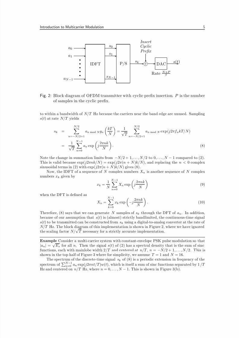
Fig. 2: Block diagram of OFDM transmitter with cyclic prefix insertion. P is the numberof samples in the cyclic prefix.

to within a bandwidth of N/T Hz because the carriers near the band edge are unused. Sampling

s(t) at rate N/T yields

sk =

N/2n=−N/2+1

an mod N gn

kT

N

=

1√T

N/2n=−N/2+1

an mod N exp( j2πf nkT/N )

=1√T

N −1n=0

an exp

j

2πnk

N

. (8)

Note the change in summation limits from −N/2 + 1, . . . , N /2 to 0, . . . , N − 1 compared to (2).This is valid because exp( j2πnk/N ) = exp( j2π(n + N )k/N ), and replacing the n < 0 complexsinusoidal terms in (2) with exp( j2π(n + N )k/N ) gives (8).

Now, the IDFT of a sequence of N complex numbers X n is another sequence of N complex

numbers xk given by

xk =1

N

N −1n=0

X n exp

j

2πnk

N

(9)

when the DFT is defined as

X n =N −1k=0

xk exp

− j

2πnk

N

. (10)

Therefore, (8) says that we can generate N samples of sk through the DFT of an. In addition,because of our assumption that s(t) is (almost) strictly bandlimited, the continuous-time signals(t) to be transmitted can be constructed from sk using a digital-to-analog converter at the rate of N/T Hz. The block diagram of this implementation is shown in Figure 2, where we have ignoredthe scaling factor N/

√T necessary for a strictly accurate implementation.

Example Consider a multi-carrier system with constant-envelope PSK pulse modulation so that|an| =

√E s for all n. Then the signal s(t) of (2) has a spectral density that is the sum of sinc

functions, each with mainlobe width 2/T and centered at n/T , n = −N/2 + 1, . . . , N /2. This isshown in the top half of Figure 3 where for simplicity, we assume T = 1 and N = 16.

The spectrum of the discrete-time signal sk of (8) is a periodic extension in frequency of the

spectrum of N −1

n=0 an exp( j2πnt/T )w(t), which is itself a sum of sinc functions separated by 1 /T Hz and centered on n/T Hz, where n = 0, . . . , N − 1. This is shown in Figure 3(b).




Next, the digital-to-analog converter (DAC) output is the lowpass filtered version of Figure 3(b)– the passband of the lowpass filter is the region between the two thick dashed lines. Clearly, if thecarriers near the edge of the passband, i.e. n = N/2 + 1, . . . , N /2 + p and n = N/2− p + 1, . . . , N /2,

are turned off, the spectra of the DAC output and s(t) will be nearly identical. This demonstratesthat the DFT/DAC combination is capable of producing an OFDM signal.

The receiver is designed to be implementable using the DFT – it is a bank of filters matchedto the nth carrier waveform gn(t) rather than to h(t) ∗ gn(t) as it should be in theory. Since gn(t)is associated with the (n mod N )th symbol, we label the matched filter outputs accordingly andfind

yn mod N =

r(t)g∗n(t)dt =

r(t)exp(− j2πf nt)dt, (11)

where again, we have left out the scaling term for simplicity. Note that in this expression, n runsfrom −N/2 + 1 through N/2. Next, since the signal component of r(t), which is h(t) ∗ s(t), isbandlimited by assumption to (−N/2T, N/2T ), we can sample r(t) at rate N/T (after lowpass

filtering) without loss of information, and express yn mod N as

yn mod N =N −1k=0

rk exp

− j

2πnk

N

(12)

to within a scale factor1.If we define n = n mod N , then n goes from 0 through N − 1, and substitution in (12) yields

yn =

N −1k=0

rk exp

− j

2πnk

N

(13)

where the right-hand side holds because of the periodicity of the complex exponential. Thereforey0 to yN −1 are obtained through the DFT of the samples r0 through rN −1, where rk = r(kT/N ).This results in the receiver structure shown in Figure 4.

2.5 The Cyclic Prefix

The question now is: how do we ensure that yn does not suffer from interference from symbolsam, m = n? The answer comes from a well-known result in digital signal processing which statesthat circular convolution in the discrete-time domain is equivalent to multiplication in the discrete-frequency domain.

To be precise, suppose xk is a length-N sequence. Its circular convolution with another se-quence hkk=0,...,N −1 is defined as

yk = xk hk =N −1

l=0

hlx(k−l) mod N =N −1

l=0

xlh(k−l) mod N . (14)

This is the same as periodically extending hl and xl to form the periodic sequences hl and xl, andthen summing hlxk−l over one period of N samples, as illustrated in Figure 5 for k = 0 and N = 3.

Then the DFT of yk, k = 0, . . . , N − 1, is Y n = H nX n where H n =N −1

k=0 hk exp(− j2πnk/N ).The proof of this result is straightforward and left as an exercise.

1 Calculating these scale factors is not important and is left to the interested reader.




−15 −10 −5 0 5 10 150

0.1

0.2

0.3

0.4

0.5

0.6

0.7

0.8

0.9

1

aN/2+1

Frequency (normalized so that T = 1)

aN/2

(a)

−25 −20 −15 −10 −5 0 5 10 15 20 250

0.1

0.2

0.3

0.4

0.5

0.6

0.7

0.8

0.9

1

a0 a

N−1

Frequency (normalized so that T = 1)

(b)

Fig. 3: (a) Spectrum of the desired OFDM baseband continuous-time signal s(t). (b)Spectrum of the DFT output before (an endless repetition of the fundamentalsegment shown in solid lines) and after (the part between the two dashed thicklines) the DAC.




s(t)E h(t) E i+ c

n(t)

Er(t)ADC

Rate (N +P )T

ERemoveCyclicPrefix

E S/P

E

E

E

DFT

E

E

E y0

y1

yN −1

r0

r1

rN −1

rk

Fig. 4: Block diagram of OFDM receiver based on the DFT.

d

d

d

hl

l 0 1 2

E

d

d

d

x−l

E

d

d

d

x−l d

d

d

d

d

d

d

d

dhl

d

d

d

d

d

d

0 1 2· · · · · ·

× × × E hk xk|k=0

Fig. 5: Circular convolution of xk and hk, both having three non-zero samples, so N =3. Note that the convolution window can be moved to span any three samplingintervals, and the result will remain the same.




In OFDM, the baseband received signal sampled at rate N/T is obtained by passing thesampled transmitted signal sk through a linear channel with discrete-time impulse response hk,and then adding receiver noise nk i.e.

rk = hk ∗ sk + nk =L−1l=0

hlsk−l + nk (15)

where ∗ denotes linear convolution. hk is obtained from the continuous-time channel response h(t)by setting t = kT/N . In fact, when L N which is the usual case, linear convolution is identicalto circular convolution, except at the beginning and end of the sequence.

To make the two operations exactly identical, we can periodically extend the input xk, asshown in Figure 6, by P samples where P ≥ L − 1. The input sequence will now have lengthN + P , so that the output sequence will have N + P + L − 1 samples. The N output samples attimes P + 1 through N + P can be shown to be the output of a circular convolution operation:

yk =

L−1

l=0

hlx(k−l) mod N = hk xk, k = P + 1, . . . , N + P. (16)

It is very important to note that the equivalence between linear and circular convolution existsonly under the following conditions:

1. The cyclic prefix is longer than the channel delay spread or P ≥ L − 1;

2. The observation window applied to the output spans the samples P + 1 through N + P –translating the window in either direction invalidates the result.

Assuming these conditions hold, we can now state the following theorem:

Theorem 1: For a discrete-time channel hk of length L, and a channel input sk that is periodicallyextended in its preamble by P

≥L

−1 samples where

s0, . . . , sN −1

= IDFT

a0, . . . , aN −1

, the

channel output rk = hk ∗ sk + nk has the property that

rk = hk sk + nk, k = P + 1, . . . , N + P, (17)

with representing circular convolution. The DFT of rP +1, . . . , rN +P is, by the duality betweencircular convolution in the time domain and multiplication in the discrete frequency domain,

y = Fr = hf a + n (18)

where all vectors have N complex elements, x y is the element-wise product of vectors x andy, Fn,k = exp( j2πnk/N ) is the DFT matrix, hf = Fh is the N th-order DFT of h and n is acircularly symmetric Gaussian vector with covariance matrix N 0I.

In scalar notation, the nth DFT output is yn = H n · an + noise, where H n is the nth DFT

coefficient of h0, . . . , hL−1,

N −L 0, . . . , 0. Since the nth “matched filter” output is independent of am,

m = n, the cyclic prefix together with the DFT/IDFT implementation of the transceiver createsN orthogonal flat-fading channels.




d

d

d

d d d d d d d d d

hl

× × × × × × × × × × × ×

xN +1−l

d d

d d

d d

d

d d

d d

d

E yN +1 = hk ∗ xk|k=N +1

(Linear convolution)

d

d

d

d d d d d d d d d

hl

× × × × × × × × × ×

xN +1−l

d d

d d d

d d

d d

d d

d

E yk = hk xk

k = 2, . . . , N + 1(Linear convolution, but theseN samples identical to outputof circular convolution.)

Fig. 6: Adding a cyclic prefix to the input signal makes linear convolution look like circularconvolution, and removes ISI in the OFDM signal. In this example, the input

sequence length is N = 10, the channel response length is L = 3. If the input hasa cyclic prefix of length L − 1 = 2, the N outputs y2, . . . , yN +1 are obtained bycircular convolution of xk and hk.




2.6 Single-Tap Equalization

Since yn = H nan + vn where E [vmv∗n] = N 0δm,n, to recover an one can estimate H n (usuallythrough the periodic transmission of known pilot symbols) and then form the statistic

an =yn

H n≈ an +

vn

H n(19)

where H n is the latest estimate of H n. A slicer is then applied to an to obtain hard decisions on an.This approach comes from minimum-distance detection applied independently to each yn, whichwill produce the minimum symbol error probability decision given that vm and vn are independent.

2.7 Loss in Spectral Efficiency

When a cyclic prefix of P samples is added to the block of N samples in time, the sampling rate (atthe DAC) needs to increase to (N + P )/T because the N + P samples still need to be transmittedover T seconds. The lowpass filter at the DAC will have a cutoff frequency of (N + P )/2T Hz.

So the spectrum of the transmitted signal with cyclic prefix inserted occupies about ( N + P )/2T ,whereas without the prefix, it occupies only N/2T Hz. In that sense, the prefix has “wasted” P/2T Hz of bandwidth since it does not carry any information and there is a fractional loss of P/(N + P )in spectral efficiency.

So it is clear that inserting the cyclic prefix to solve the ISI problem comes at a price, and inpractice we always strive to make P as small a fraction of N as possible to limit the wastage of bandwidth.

3 Advanced Topics

3.1 Frequency Offset in a Multi-User OFDMA Uplink

OFDM can be used to provide channel access to a number of users, much like FDMA (frequency

division multi-access) except that frequency bands used by different users need not be separated bya guard band. This gives OFDMA a potentially higher spectral efficiency than FDMA. However,OFDMA is very sensitive to frequency offsets, which may come from mismatches in the localoscillators at transmitter and receiver ends of the link, or Doppler shifts in the case of mobileapplications. We now quantify the effects of frequency offsets.

3.1.1 Signal Model

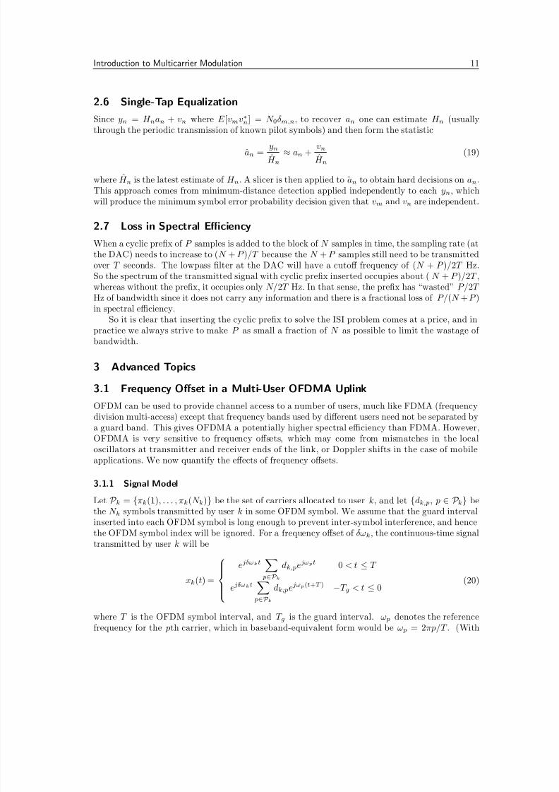
Let P k = πk(1), . . . , πk(N k) be the set of carriers allocated to user k, and let dk,p, p ∈ P k bethe N k symbols transmitted by user k in some OFDM symbol. We assume that the guard intervalinserted into each OFDM symbol is long enough to prevent inter-symbol interference, and hencethe OFDM symbol index will be ignored. For a frequency offset of δωk, the continuous-time signaltransmitted by user k will be

xk(t) =

ejδωkt p∈Pk

dk,pejωpt 0 < t ≤ T

ejδωkt p∈Pk

dk,pejωp(t+T ) −T g < t ≤ 0(20)

where T is the OFDM symbol interval, and T g is the guard interval. ω p denotes the referencefrequency for the pth carrier, which in baseband-equivalent form would be ω p = 2πp/T . (With




pulse shaping to limit the bandwidth of the transmitted signal, the actual transmitted signal willbe xk(t) ∗ p(t) where p(t) is the impulse response of the pulse-shaping filter. However, since p(t)can be absorbed into the channel, we lose no generality in treating xk(t) as the transmitted signal

and gain notational simplicity.)The signal received from user k will be the convolution of xk(t) with the kth channel impulseresponse hk(t), or

yk(t) = xk(t) ∗ hk(t). (21)

If we sample the received signal above its Nyquist rate and discard the cyclic prefix, we find thatthe linear convolution becomes equivalent to a circular or periodic convolution, or

yk[n] = xk[n] hk[n] (22)

with n = 0, . . . , N − 1 where N is the number of samples in T seconds, and xk[n] = xk(nT/N ).Note that the sampling rate is N/T – if the carriers near the band edges are not used, then the one-sided bandwidth of the OFDM signal is N c/2T , and hence N = N c will yield sufficient statisticsfor the detection of all transmitted symbols. We therefore assume that N = N c.

The discrete-time Fourier transform (DTFT) of yk[n] is simply the product of the DTFT’s of xk[n] and hk[n], or

Y k(Ω) = X k(Ω)H k(Ω). (23)

We can show from first principles that X k(F ) is a sum of frequency-shifted Dirichlet functions2:

X k(Ω) = p∈Pk

dk,pdrcl (Ω − (δωk + ω p)T /N c, N c) (24)

where

drcl(x, N )=

sin(N x/2)

N sin(x/2). (25)

To be more concise, we can write X k(Ω) =

p∈Pk

dk,pS k,p(Ω).The complete received signal in the frequency domain is therefore

Y (Ω) =

Kk=1

Y k(Ω) + W (Ω) =

Kk=1

H k(Ω)X k(Ω) + W (Ω) (26)

=Kk=1

H k(Ω) p∈Pk

dk,pS k,p(Ω) + W (Ω), (27)

where W (Ω) is complex AWGN. In vector notation, treating Y (Ω), −π < Ω ≤ π as a vector y andsimilarly converting all other frequency functions to vectors, we have

y =Kk=1

HkSkdk + w (28)

where Hk = diag(hk), hk is the vector representing H k(Ω), Sk = [sk,πk(1), . . . , sk,πk(N k)] anddk = [dk,πk(1), . . . , dk,πk(N k)]. Finally, we can also write

y = HSd + w (29)

with H = [H1, . . . , HK], S = diag[S1, . . . , SK ] and d = [dT 1 , . . . , dT

K ]T .

2 Complex scaling term ignored.




−4 −3 −2 −1 0 1 2 3 4−0.4

−0.2

0

0.2

0.4

0.6

0.8

1

Ω (rad/s)

Fig. 7: 15 instances of S k,p(Ω), with zero frequency offsets. N c = 16.

3.1.2 Interpretations

The Dirichlet function defined in (25) is central to our analysis so we should study it more closely.The following properties are important:

1. drcl(x, N ) has zero crossings at x = 2πp/N for integer p;

2. drcl(0, N ) = 1.

In this sense, the Dirichlet function is similar to the sinc function sinc(N x/2) where sinc(x) =sin x/x. In fact, a plot of the two functions would be virtually indistinguishable.

If all users transmit over AWGN channels with unit gain, i.e. hk = 1, then the frequency-domain received signal will be a linear combination of Dirichlet functions, plotted in Figure 7 wherewe assumed 16 carriers. This is the spectrum or discrete-time Fourier transform (DTFT) of thesequence y[n].

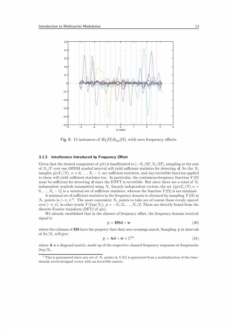
When the channels are frequency selective, the received signal will be a linear combinationof distorted versions of these Dirichlet functions, namely H k(Ω)S k,p(Ω), such as those plotted inFigure 8. In this figure, the vertical lines indicate the frequencies Ω = 2πp/N c – notice that at

these frequencies, all but one of the functions are zero. This is due to these frequencies being atthe zero crossings of the shifted Dirichlet functions of Figure 7.In the presence of frequency offsets, the received signal becomes a linear combination of shifted

Dirichlet functions, which no longer all have zero crossings at Ω = 2πp/N c. For instance, with fourusers each having its own frequency offset, S k,p(Ω) will look like the curves in Figure 9.




−4 −3 −2 −1 0 1 2 3 4−0.5

−0.4

−0.3

−0.2

−0.1

0

0.1

0.2

0.3

0.4

0.5

Ω (rad/s)

Fig. 8: 15 instances of H k(Ω)S k,p(Ω), with zero frequency offsets.

3.1.3 Interference Introduced by Frequency Offset

Given that the desired component of y(t) is bandlimited to [−N c/2T, N c/2T ], sampling at the rateof N c/T over one OFDM symbol interval will yield sufficient statistics for detecting d. So the N c

samples y(nT c/N ), n = 0, . . . , N c − 1, are sufficient statistics, and any invertible function appliedto them will yield sufficient statistics too. In particular, the continuous-frequency function Y (Ω)must be sufficient for detecting d since the DTFT is invertible. But since there are a total of N cindependent symbols transmitted using N c linearly independent vectors, the set y(nT c/N ), n =0, . . . , N c − 1 is a minimal set of sufficient statistics, whereas the function Y (Ω) is not minimal.

A minimal set of sufficient statistics in the frequency domain is obtained by sampling Y (Ω) atN c points in [−π, π]3. The most convenient N c points to take are of course those evenly spacedover [−π, π], in other words Y (2πp/N c), p = −N c/2, . . . , N c/2. These are directly found from thediscrete Fourier transform (DFT) of y[n].

We already established that in the absence of frequency offset, the frequency-domain receivedsignal is

y = HSd + w (30)

where the columns of HS have the property that their zero crossings match. Sampling y at intervalsof 2π/N c will givey = Ad + w ∈ CN c (31)

where A is a diagonal matrix, made up of the respective channel frequency responses at frequencies2πp/N c.

3 This is guaranteed since any set of N c points in Y (Ω) is generated from a multiplication of the time-domain received-signal vector with an invertible matrix.




−2 −1.5 −1 −0.5 0 0.5 1 1.5 2

−0.2

0

0.2

0.4

0.6

0.8

1

Ω (rad/s)

Fig. 9: Some of the frequency-domain basis functions for xk[n], with frequency offset. Ob-serve that at frequencies Ω = 2πp/N c, marked by the dashed vertical lines, severalof these functions will be non-zero, in contrast to the zero offset case.




Since A is diagonal, there is no interference in the minimal frequency-domain sufficient statisticsy, and optimal detection proceeds on a per-user basis.

When frequency offset is present, then the columns of HS do not have the same zero crossings

(except those belonging to the same user), as we can see from Figure 9. Uniform sampling of Y (Ω)will then give (31) but with a non-diagonal A, indicating non-zero multi-user interference.The most important point proven here is that frequency offset in an OFDMA system creates

multi-user interference. Whether the offsets can be estimated and then used in multi-user detection,or whether practical frequency offsets are small enough to avoid serious performance issues aretopics for future discussion.

ofdmnotes must read

Documents