ocean optics protocols for satellite ocean color … vi: special topics in ocean optics protocols,...

NASA/TM-2004-

Ocean Optics Protocols For Satellite Ocean Color Sensor Validation, Revision 5,

Volume VI: Special Topics in Ocean Optics Protocols, Part 2

James L. Mueller and Giulietta S. Fargion and Charles R. McClain, Editors J. L. Mueller, S. W. Brown, D. K. Clark, B. C. Johnson, H. Yoon, K. R. Lykke, S. J. Flora, M. E. Feinholz, N. Souaidia, C. Pietras, T. C. Stone, M. A. Yarbrough, Y. S. Kim, R. A. Barnes, Authors. National Aeronautics and Space administration Goddard Space Flight Space Center Greenbelt, Maryland 20771 February 2004

NASA/TM-2004- James L. Mueller1 and Giulietta S. Fargion2 Editors

Ocean Optics Protocols For Satellite Ocean Color Sensor Validation, Revision 5, Volume VI, Part 2:

Special Topics in Ocean Optics Protocols, Part 2 James L Mueller, CHORS, San Diego State University, San Diego, California Giulietta S. Fargion, Science Applications International Corporation, Beltsville, Maryland Charles R. McClain, NASA Goddard Space Flight Center, Greenbelt, Maryland B. Carol Johnson, Steven W. Brown, Howard Yoon, Keith Lykke, Nordine Souaidia, National Institute of

Standards and Technology, Gaithersburg Maryland Dennis K. Clark, National Oceanic and Atmospheric Administration, National Environmental Satellite

Data and Information Service, Camp Springs, Maryland Stephanie Flora, Michael E. Feinholz, Mark Yarbrough, Moss Landing Marine Laboratories, San Jose

State University, Moss Landing, California Yong Sung Kim, STG Inc., Rockville, Maryland Christophe Pietras, Robert A. Barnes, SAIC General Sciences Corporation, Beltsville, Maryland Thomas C. Stone, United States Geological Survey, Flagstaff, Arizona National Aeronautics and Space administration Goddard Space Flight Space Center Greenbelt, Maryland 20771 February 2004

Ocean Optics Protocols For Satellite Ocean Color Sensor Validation, Revision 5 Volume VI, Part 2: Special Topics in Ocean Optics Protocols

i

Preface To Revision 5

This document stipulates protocols for measuring bio-optical and radiometric data for the Sensor Intercomparison and Merger for Biological and Interdisciplinary Oceanic Studies (SIMBIOS) Project activities and algorithm development. The document is organized into 6 separate volumes, and in Revision 5, Volume VI is divided into 2 parts. Revision 5 consists of a new version of Volume V (Biogeochemical and Bio-Optical Properties) that supercedes and replaces Volume V (Revision 4), and new additions to Volume VI (Special Topics) are issued as Part 2 of that volume. The currently effective ocean optics protocol volumes, as of Revision 5, are:

Ocean Optics Protocols for Satellite Ocean Color Sensor Validation Volume I: Introduction, Background and Conventions (Rev. 4) Volume II: Instrument Specifications, Characterization and Calibration (Rev. 4) Volume III: Radiometric Measurements and Data Analysis Methods (Rev. 4) Volume IV: Inherent Optical Properties: Instruments, Characterization, Field Measurements and Data

Analysis Protocols (Rev. 4 and Erratum 1 dated 28 Aug. 2003) Volume V: Biogeochemical and Bio-Optical Measurements and Data Analysis Methods (Rev. 5) Volume VI: Special Topics in Ocean Optics Protocols and Appendices (Rev. 4) Volume VI, Part 2: Special Topics in Ocean Optics Protocols, Part 2 (Rev. 5)

Volume V (Revision 5): This volume is issued as a complete replacement for Volume V (Revision 4). The overview chapter (Chapter 1) briefly reviews biogeochemical and bio-optical measurements, and points to literature covering methods for measuring these variables. Detailed protocols for HPLC measurement of phytoplankton pigment concentrations are given in Chapter 2, and the Revision 5 version incorporates the Erratum issued in June 2003 to modify the HPLC protocols related to water retention by GF/F filters. Chapter 3 gives protocols for Fluorometric measurement of chlorophyll a concentration, and is carried over unchanged from Revision 4. Chapter 4 is a new addition which describes protocols for determining backscattering by Coccolithophorids and detached Coccoliths.

Volume VI, Part 2 (Revision 5): This volume supplements the 5 chapters of Volume VI (Rev. 4), adding two new “Special Topics” chapters:

• Chapter 6 briefly reviews recent progress in protocols for instrument self shading corrections to in-water upwelled radiance measurements;

• Chapter 7 reviews recent advances in radiometric characterization and measurement methods that are directly relevant to ocean color remote sensing and validation of satellite ocean color sensors.

This technical report is not meant as a substitute for scientific literature. Instead, it will provide a ready and responsive vehicle for the multitude of technical reports issued by an operational Project. The contributions are published as submitted, after only minor editing to correct obvious grammatical or clerical errors.


ii

Preface to Revision 4

This document stipulates protocols for measuring bio-optical and radiometric data for the Sensor Intercomparison and Merger for Biological and Interdisciplinary Oceanic Studies (SIMBIOS) Project activities and algorithm development. The document is organized into 7 separate volumes as:

Ocean Optics Protocols for Satellite Ocean Color Sensor Validation, Revision 4 Volume I: Introduction, Background and Conventions Volume II: Instrument Specifications, Characterization and Calibration Volume III: Radiometric Measurements and Data Analysis Methods Volume IV: Inherent Optical Properties: Instruments, Characterization, Field Measurements and Data

Analysis Protocols Volume V: Biogeochemical and Bio-Optical Measurements and Data Analysis Methods Volume VI: Special Topics in Ocean Optics Protocols Volume VII: Appendices

The earlier version of Ocean Optics Protocols for Satellite Ocean Color Sensor Validation, Revision 3 (Mueller and Fargion 2002, Volumes 1 and 2) is entirely superseded by the seven Volumes of Revision 4 listed above.

The new multi-volume format for publishing the ocean optics protocols is intended to allow timely future revisions to be made reflecting important evolution of instruments and methods in some areas, without reissuing the entire document. Over the years, as existing protocols were revised, or expanded for clarification, and new protocol topics were added, the ocean optics protocol document has grown from 45pp (Mueller and Austin 1992) to 308pp in Revision 3 (Mueller and Fargion 2002). This rate of growth continues in Revision 4. The writing and editorial tasks needed to publish each revised version of the protocol manual as a single document has become progressively more difficult as its size increases. Chapters that change but little, must nevertheless be rewritten for each revision to reflect relatively minor changes in, e.g., cross-referencing and to maintain self-contained consistency in the protocol manual. More critically, as it grows bigger, the book becomes more difficult to use by its intended audience. A massive new protocol manual is difficult for a reader to peruse thoroughly enough to stay current with and apply important new material and revisions it may contain. Many people simply find it too time consuming to keep up with changing protocols presented in this format - which may explain why some relatively recent technical reports and journal articles cite Mueller and Austin (1995), rather than the then current, more correct protocol document. It is hoped that the new format will improve community access to current protocols by stabilizing those volumes and chapters that do not change significantly over periods of several years, and introducing most new major revisions as new chapters to be added to an existing volume without revision of its previous contents.

The relationships between the Revision 4 chapters of each protocol volume and those of Revision 3 (Mueller and Fargion 2002), and the topics new chapters, are briefly summarized below:

Volume I: This volume covers perspectives on ocean color research and validation (Chapter 1), fundamental definitions, terminology, relationships and conventions used throughout the protocol document (Chapter 2), requirements for specific in situ observations (Chapter 3), and general protocols for field measurements, metadata, logbooks, sampling strategies, and data archival (Chapter 4). Chapters 1, 2 and 3 of Volume I correspond directly to Chapters 1, 2 and 3 of Revision 3 with no substantive changes. Two new variables, Particulate Organic Carbon (POC) and Particle Size Distribution (PSD) have been added to Tables 3.1 and 3.2 and the related discussion in Section 3.4; protocols covering these measurements will be added in a subsequent revision to Volume V (see below). Chapter 4 of Volume I combines material from Chapter 9 of Revision 3 with a brief summary of SeaBASS policy and archival requirements (detailed SeaBASS information in Chapter 18 and Appendix B of Revision 3 has been separated from the optics protocols).

Volume II: The chapters of this volume review instrument performance characteristics required for in situ observations to support validation (Chapter 1), detailed instrument specifications and underlying rationale (Chapter 2) and protocols for instrument calibration and characterization standards and methods (Chapters 3 through 5). Chapters 1 through 5 of Volume II correspond directly to Revision 3 chapters 4 through 8, respectively, with only minor modifications.


iii

Volume III: The chapters of this volume briefly review methods used in the field to make the in situ radiometric measurements for ocean color validation, together with methods of analyzing the data (Chapter 1), detailed measurement and data analysis protocols for in-water radiometric profiles (Chapter 2), above water measurements of remote sensing reflectance (Chapter III-3), determinations of exact normalized water-leaving radiance (Chapter 4), and atmospheric radiometric measurements to determine aerosol optical thickness and sky radiance distributions (Chapter 5). Chapter 1 is adapted from relevant portions of Chapter 9 in Revision 3. Chapter 2 of Volume III corresponds to Chapter 10 of Revision 3, and Chapters 3 through 5 to Revision 3 Chapters 12 through 14, respectively. Aside from reorganization, there are no changes in the protocols presented in this volume.

Volume IV: This volume includes a chapter reviewing the scope of inherent optical properties (IOP) measurements (Chapter 1), followed by 4 chapters giving detailed calibration, measurement and analysis protocols for the beam attenuation coefficient (Chapter 2), the volume absorption coefficient measured in situ (Chapter 3), laboratory measurements of the volume absorption coefficients from discrete filtered seawater samples (Chapter 4), and in situ measurements of the volume scattering function, including determinations of the backscattering coefficient (Chapter 5). Chapter 4 of Volume IV is a slightly revised version of Chapter 15 in Revision 3, while the remaining chapters of this volume are entirely new contributions to the ocean optics protocols. These new chapters may be significantly revised in the future, given the rapidly developing state-of-the-art in IOP measurement instruments and methods.

Volume V: The overview chapter (Chapter 1) briefly reviews biogeochemical and bio-optical measurements, and points to literature covering methods for measuring these variables; some of the material in this overview is drawn from Chapter 9 of Revision 3. Detailed protocols for HPLC measurement of phytoplankton pigment concentrations are given in Chapter 2, which differs from Chapter 16 of Revision 3 only by its specification of a new solvent program. Chapter 3 gives protocols for Fluorometric measurement of chlorophyll a concentration, and is not significantly changed from Chapter 17of Revision 3. New chapters covering protocols for measuring, Phycoerythrin concentrations, Particle Size Distribution (PSD) and Particulate Organic Carbon (POC) concentrations are likely future additions to this volume.

Volume VI: This volume gathers chapters covering more specialized topics in the ocean optics protocols. Chapter 1 introduces these special topics in the context of the overall protocols. Chapter 2 is a reformatted, but otherwise unchanged, version of Chapter 11 in Revision 3 describing specialized protocols used for radiometric measurements associated with the Marine Optical Buoy (MOBY) ocean color vicarious calibration observatory. The remaining chapters are new in Revision 4 and cover protocols for radiometric and bio-optical measurements from moored and drifting buoys (Chapter 3), ocean color measurements from aircraft (Chapter 4), and methods and results using LASER sources for stray-light characterization and correction of the MOBY spectrographs (Chapter 5). In the next few years, it is likely that most new additions to the protocols will appear as chapters added to this volume. This volume also collects appendices of useful information. Appendix A is an updated version of Appendix A in Revision 3 summarizing characteristics of past, present and future satellite ocean color missions. Appendix B is the List of Acronyms used in the report and is an updated version of Appenix C in Revision 3. Similarly, Appendix C, the list of Frequently Used Symbols, is an updated version of Appendix D from Rev. 3. The SeaBASS file format information given in Appendix B of Revision 3 has been removed from the protocols and is promulgated separately by the SIMBIOS Project.

In the Revision 4 multi-volume format of the ocean optics protocols, Volumes I, II and III are unlikely to require significant changes for several years. The chapters of Volume IV may require near term revisions to reflect the rapidly evolving state-of-the-art in measurements of inherent optical properties, particularly concerning instruments and methods for measuring the Volume Scattering Function of seawater. It is anticipated that new chapters will be also be added to Volumes V and VI in Revision 5 (2003).

This technical report is not meant as a substitute for scientific literature. Instead, it will provide a ready and responsive vehicle for the multitude of technical reports issued by an operational Project. The contributions are published as submitted, after only minor editing to correct obvious grammatical or clerical errors.


iv

Table of Contents

CHAPTER 6....................................................................................................................................................................1

SHADOW CORRECTIONS TO IN-WATER UPWELLED RADIANCE MEASUREMENTS: A STATUS REVIEW

6.1 INTRODUCTION ........................................................................................................................................... 1 6.2 PROGRESS TOWARD PLATFORM SHADING CORRECTIONS .................................................... 1 6.3 INSTRUMENT SELF -SHADING CORRECTIONS ............................................................................... 2

Protocols for Circularly Concentric Instrument Self-Shading Geometries...........................................2 Non-Concentric and Irregularly Shaped Instrument Geometries...........................................................3 A simple “effective radius” adaptation of the GD protocol for MOBY and MOS ...............................5

6.4 DISCUSSION AND FUTURE DIRECTIONS.......................................................................................... 6 REFERENCES........................................................................................................................................................ 6

CHAPTER 7....................................................................................................................................................................8

ADVANCES IN RADIOMETRY FOR OCEAN COLOR 7.1 INTRODUCTION ........................................................................................................................................... 8 7.2. ADVANCED CALIBRATION SOURCES ............................................................................................... 9

The 2000 NIST irradiance scale..................................................................................................................10 Solid-state, ocean color radiance calibration source..............................................................................12

7.3. NIST FACILITY FOR SPECTRAL IRRADIANCE AND RADIANCE RESPONSIVITY CALIBRATIONS USING UNIFORM SOURCES (SIRCUS) .................................................................... 12

Sun photometer and sky radiometer calibration comparisons between SIRCUS and NASA’s Goddard Space Flight Center...................................................................................................................................................14 Stray light characterization and correction of spectrographs...............................................................18 Least-squares matrix solutions for spectrograph stray light characterization...................................21 Stray light corrections to MOBY upwelled radiance measurements using different slit response function models..............................................................................................................................................................23 Stray light, ocean color and bio-optical algorithms................................................................................26

7.4 LUNAR RADIOMETRY............................................................................................................................. 29 7.5. SUMMARY................................................................................................................................................... 32 ACKNOWLEDGEMENTS ................................................................................................................................ 32 REFERENCES...................................................................................................................................................... 32


1

Chapter 6

Shadow Corrections to In-Water Upwelled Radiance Measurements: A Status Review

James L. Mueller Center for Hydro-Optics and Remote Sensing, San Diego State University, California

6.1 INTRODUCTION Shadows cast by ships, other platforms from which instruments are deployed, and instrument housings can

cause in-water measurements of ( )u ,L z λ to be systematically offset below the true values. These shadow induced

measurement errors propagate directly to in-water determinations of water-leaving radiance ( )WL λ and exact

normalized water-leaving radiance ( )exWNL λ , as well.

The current protocol concerning ship, or platform, shadowing of ( )u ,L z λ measurements is essentially to make

the radiometric profile measurement far enough away from the ship to avoid the phenomenon altogether (Mueller 2003, Sect. 2.2); the recommended distance is based on the ship shadow model of Gordon (1985). Current practice is to use tethered, free-falling radiometers drifted well away from the ship, but there are some circumstances when platform shadow effects cannot be completely avoided. Gordon (1985) presented his modeling results to illustrate the magnitude of ship shadow artifacts on downwelled irradiance and upwelled irradiance and radiance; he did not propose the use of this model as a basis for correcting the offsets. There has been significant recent progress in using backward Monte Carlo models (Gordon 1985; Mobley 1994) to develop shading corrections to radiometric profiles measured from a very large offshore tower (Zibordi et al. 1999; Doyle and Zibordi 2002; Doyle et al. 2003). These developments are briefly reviewed in Section 6.2, below.

It is impossible to avoid self-shading of in-water ( )u ,L z λ measurements by the instrument itself. Because the

magnitude of self-shading error depends directly on the diameter of a radiometer, however, manufacturers have significantly reduced the diameters of commercially available in-water radiance instruments over the past decade. Moreover, some instrument use fiber optics to place the upwelled irradiance and radiance sensor apertures on arms away from the main instrument housing, a design configuration that can significantly reduce self-shading artifacts (e.g. Piskozub et al. 2000; Clark et al. 2003). A provisional protocol for instrument self-shading corrections, described in Mueller (2003, Sect. 2.3), is based on the model of Gordon and Ding (1992) and the initial experimental verification of the model by Zibordi and Ferrari (1995). Other experiments (Aas and Korsbo 1997) also suggest that the present instrument self-shading protocol based on the Gordon and Ding (1992) model appears to work reasonably well for cylindrical instruments having radiance, or irradiance, apertures centered in the lower face. Leathers et al. (2001) developed an extension of the Gordon and Ding (1992) model for shading by a cylindrical instrument extending downward a certain distance beneath a buoy of larger diameter. On the other hand, there are many instrument and buoy radiance sensor configurations that do not closely approximate the circularly concentric geometry underlying the Gordon and Ding (1992) and Leathers et al. (2001) models. These aspects of the instrument self-shading protocols, and possible pathways to more general correction algorithms, are briefly reviewed below in Section 6.3.

6.2 PROGRESS TOWARD PLATFORM SHADING CORRECTIONS A large offshore tower, the Acqua Alta Oceanographic Tower located near Venice, Italy in the Adriatic Sea near

Venice, Italy, is used to support satellite ocean color sensor validation. As a critical part of this project, radiometric profiles are routinely measured close enough to the massive tower structure that downwelled spectral irradiance and upwelled spectral irradiance and radiance measurements are significantly perturbed by its shadow. To correct for these shadow perturbation, Dr. Giuseppe Zibordi – the project leader – and his colleagues developed sophisticated Monte Carlo radiative transfer model of the coupled atmosphere and ocean, and applied it to the task of generating


2

lookup-tables giving tower shading corrections to downwelled irradiance and upwelled irradiance and radiance (Zibordi et al. 1999; Doyle and Zibordi 2002). The 3-dimensional model includes a close geometric approximation to the tower structure, a reflecting bottom (at a depth of approximately 17 m), vertical profiles of inherent optical properties (IOP), and atmospheric total and aerosol optical thickness and sky-radiance distribution measured using a sun photometer. The water IOP and atmospheric variables are routinely measured, together with the radiometric profiles for which shading corrections must be generated. The model was run through an extremely large number of simulations to generate lookup tables of modeled corrections for varying solar azimuth and zenith angles, aerosol optical thickness and scattering phase function, IOP profiles, and varying horizontal distance of the profiler from the tower. The range and resolution of these governing variables, which are used as inputs to the resulting correction tables, were derived from the multi-year record of measurements on the tower. The correction tables generated by the model have been experimentally validated through comparisons with radiometric profiles measured at varying distances from the tower, including simultaneous measurements using multiple profiling packages (Doyle et al. 2003).

It is problematic whether the impressively successful platform shading correction scheme developed for the Acqua Alta Oceanographic Tower could be practically extended to derive ship shadow corrections. The much larger variability in possible geometric configurations for different ships oriented in varying azimuthal direction relative to the sun would seem to preclude this possibility (at least in the immediate future).

6.3 INSTRUMENT SELF-SHADING CORRECTIONS

Protocols for Circularly Concentric Instrument Self-Shading Geometries Gordon and Ding (1992), henceforth referred to as “GD”, represented an in-water radiometer’s housing as a flat

disc of radius r. They used backward Monte-Carlo simulations (Gordon 1985; Mobley 1994) to model the offsets that would be introduced by the disk’s shadow on upwelled irradiance and radiance measurements by sensors mounted concentrically under the disk. Separate sets of simulations were run for irradiance and radiance sensor apertures that fill the entire disk, and in each case for a point detector. Each set of simulations included varying specifications of solar zenith angles oθ , absorption coefficients ( )a λ , scattering coefficients ( )b λ , and scattering

phase functions ( );β λ ψ% , where ψ is the scattering angle. GD considered only vertically homogeneous IOP, and

since they limited their model to circularly concentric geometry, solar azimuth angle oφ and instrument azimuth directional orientation were not a factor. GD determined that, at least for Case 1 waters, the self-shading magnitude depends primarily on the product ( )a rλ , and is relatively insensitive to the detailed shape of ( );β λ ψ% . This finding

should be further investigated, however. Doyle and Zibordi (2002) found that platform corrections were sensitive at the 2 % level to variations in the scattering phase function models. Moreover, Mobley et al. (2002) found that good agreement between measured and modeled upwelled radiance required the use, in the radiative transfer model, of a phase function having a backscattering fraction consistent with that measured using a volume scattering function sensor.

For the case of direct sunlight and b a= , GD showed that the approximate relative shading effect for upwelled

radiance and a point sensor can be written analytically as o

2tan1

ar

e−

′θε = − , where o′θ is the refracted solar zenith

angle. They then assumed that for the more general case of b a∼ that they could substitute an unknown coefficient

suno

2 for

tan′κ

′θ and write sun1 are ′−κε = − . GD then fit the parameter sun otan′ ′κ θ to the values of ε determined using

the subset of backward Monte Carlo simulations at each oθ . The same form of ε was assumed for the other direct sun cases (point source irradiance, and full-disk radiance and irradiance, sensors), and for all 4 sensor types and coefficients sky

′κ assuming a uniform distribution of skylight.

Zibordi and Ferrari (1995) measured upwelled radiance and irradiance in a lake at several different solar zenith angles using a fiber optic probe placed just beneath the water surface. Disks of varying diameter were attached to the probe to simulate shading by larger instruments. Their comparisons between self-shading measurements and GD predictions agreed in all cases within < 5 %. Based on this anecdotal confirmation of GD for ( ) 0.1a rλ ≤ , the


3

model was adopted as the basis for a standard, but provisional, self-shading correction protocol (Mueller 2003). More recently, the results of radiance sensor self-shading experiments by Aas and Korsbo (1997) demonstrated < 5 % agreement between their measurements and the GD model over the extended range ( ) 0.5a rλ ≤ . To develop

the current instrument self-shading protocol (Mueller 2003), each set of tabulated GD values of sun′κ was fit as a

function of oθ (in degrees) using linear regression, and coefficients sun′κ and sky′κ were each interpolated between

the GD full-disk sensor and point-sensor values according to the ratio of actual sensor aperture radius to instrument

radius arr

. The resulting self-shading algorithms for upwelled radiance and irradiance, as reflected in the current

protocols, are described in detail in Vol. III, Chapter 2, of the current Ocean Optics Protocols (Mueller 2003).

Leathers et al. (2001) extended the GD type of model to develop self-shading corrections for a cylindrical instrument protruding downward into the water below a buoy of larger radius. The particular buoyed instrument they considered is circularly concentric, the instrument housing has a radius of 4.4 cm and extends to a water depth of 60 cm, and the buoy has a radius of 15 cm and extends 12 cm below the sea surface. Their model results include the vertical extents of the buoy and instrument, and include also the effects of a shallow, reflecting seafloor. For optically deep water masses, their modeled corrections fall between the GD corrections for disks of 15 cm and 5 cm, and approach the 5 cm GD correction in very turbid water. They provide tabulated values and a protocol for self-shading corrections that represent a significant improvement over the GD protocol for this specific buoyed radiance sensor configuration (i.e. instrument and buoy dimensions in water).

Non-Concentric and Irregularly Shaped Instrument Geometries

The GD instrument self-shading analysis, and the resulting model and protocol algorithm, were derived for a conceptual “instrument housing” consisting of an opaque, flat, circular disk having a radiance (or irradiance) sensor, also with a circular cross section, placed concentrically on the underside of the disc. They did not consider instrument housings with finite vertical size (e.g. a cylinder), horizontal cross sections of non-circular shapes, or radiance aperture locations that are not centered concentrically in the base of an instrument housing.

There are many in-water radiance instruments, including as “instruments” radiance sensors mounted on bio-optical buoys, that do not conform to the GD concentric shading geometry. Important exceptions to this concentric viewing geometry, include:

1. A nadir-viewing radiance sensor aperture located under a rectangular boom of typical length 1 m to 2 m and width of order 5 cm to 10 cm. Such a long, narrow, horizontally oriented boom is used, e.g. on MOBY (Figure 6.1), to place the radiometric sensors away from shadows and reflections from the flotation buoy. The sensor apertures are typically located within a few cm of the outer end of the boom. The shadow cast by the boom will vary with the azimuth angle between the boom direction and the sun, and the boom orientation direction must be measured if the shape of the boom shadow is to be considered.

2. A nadir-viewing detector located away from the center of a cylindrical instrument housing [e.g. the MOS profiling radiometer (Clark et al. 2003)] with diameters ranging from 10 cm to 50 cm (Fig. 6.2), or buoy hull (diameters between 0.5 m and 3 m). In many such cases, e.g. the MOS profiling radiometer (Clark et al. 2003) and several of the bio-optical buoys illustrated in Kuwahara et al. (2003), the motivation is to orient the platform so that the sensor aperture offset is generally in the direction of the solar azimuth, in the hope of thus reducing the influence of self-shading. This, of course, presupposes that the sensor-offset azimuth is known at the time of the measurement.

3. A radiance sensor viewing upwelled radiance at a nadir-angle away from zero, again located under, and towards one edge of, a buoy hull having a circular horizontal cross-section. This configuration has been employed in several moored and drifting buoy arrays, e.g. Fig. 3a in Kuwahara et al. (2003), with the intent of further reducing platform self-shading. This viewing geometry may indeed result in less shadowing than nadir viewing geometry, but it also introduces asymmetric bidirectionality associated with the ocean IOP (Morel and Mueller 2003).


4

To implement a self-shading correction algrorithm for any of the asymmetric instrument/aperture geometries described above, it is obviously necessary to use a compass to determine the azimuth angles of the radiance sensor offset, and for non-nadir views, the viewing direction.

Figure 6.1: Schematic diagram showing the dependence of relative azimuth angles of MOBY boom orientation and the sun on the effective “radius” for shading of the direct solar beam by the boom.

Figure 6.2: MOS offset aperture geometry, showing reff as the distance to the edge of the instrument housing in the direction of the solar azimuth. The positive x-axis is aligned pointing toward the sun, so that reff also points toward the sun and is parallel to the x-axis. The aperture-offset distance from

the center is denoted rs, while ri is the radius of the instrument housing.


5

A simple “effective radius” adaptation of the GD protocol for MOBY and MOS

To derive a simple, approximate means of accounting for MOBY and MOS shadowing cross-section geometries in cloud-free conditions and Case-1 waters, it is assumed that the shadowing effect is dominated by blocking the direct solar beam, an effect that can be easily calculated from the distance effr between the aperture center and the

edge of the instrument in the direction of the sun. We then assume that the shading of diffuse sky radiance by an

arbitrary shading cross section is not “much” different than that of a circular disk of radius effr . The coordinate

system is rotated with the positive x-axis aligned with the solar azimuth direction. Given azimuth angles of the sun

oφ and standoff arm direction aφ , measured with a compass in earth coordinates, the sun-relative azimuth

direction of the optical arm is determined as a a oϕ = φ − φ . With reference to Fig. 6.1, the angular intervals

between the extended centerline and the corners of the outer end of the boom are labeled c∆ϕ . The horizontal

width of the standoff arm is denoted or . The distance from the origin (aperture center) to the edge of the arm along

the positive x-axis (directly toward the sun) is shown as effr , the “effective distance” to the position on the edge of

the beam that casts the shadow of the direct solar beam into the optical path immediately below the radiance

aperture. When the arm direction aϕ is within c∆ϕ of the solar azimuth, the effective distance is assumed to be

approximately constant at 1r (although not shown in Fig. 1, the end of the standoff arm is slightly rounded).

Therefore, the “effective radius” for any arm direction may be determined as

1 a c

eff o

a

;

; otherwisesin

rrr

ϕ ≤ ∆ϕ ϕ

= . (6.1)

For the MOS (Fig. 6.2), or a buoy with a nadir-viewing radiance aperture near one edge, the origin of the coordinate system is located at the center of the circular base of the instrument housing, and the x-axis is pointed toward the sun so that o 0ϕ = . The location axv of the radiance aperture is shown offset from the origin by

distance sr in direction aϕ . The vector pointing from the aperture center toward the sun intersects the edge of the

instrument housing at distance effr in position pxv , or in polar coordinates ( )i pr ,ϕ . Given the great distance of the

sun, the parallax effect of the solar view between the origin and axv is entirely negligible so that the vector p a−x xv v

is parallel to the x-axis. With this choice of coordinates, a py y= and eff p ar x x= − . First, the coordinates of axv

are determined as

a s a a s ar cos , and r sin .x y= ϕ = ϕ (6.2)

Since a py y= we have that

1 1a s

p ai i

rsin sin sin

r ry− −

ϕ = = ϕ

. (6.3)

It follows that

p i pr cosx = ϕ , (6.4)

and finally the MOS effective radius is determined as

eff p a .r x x= − (6.5)


6

An alternative solution for eff p ar = −x xv v may be obtained directly in earth coordinates using the quadratic

equation, but the above solution in the rotated coordinate system is more easily visualized.

In either case, effr is substituted for the instrument radius in the standard GD protocol described in Mueller

(2003). This “quick and dirty” approximation is motivated entirely by the intuitive idea that its use will, as a minimum, adjust the GD model in the right direction for non-concentric geometry. It is certainly not a correct model construct, however, as it improperly represents the shadowing of the diffuse skylight component built in to the GD model fit. An investigation is currently ongoing to evaluate these geometric aspects of the self-shading problem via new backward Monte Carlo calculations (Gordon 1985; Mobley 1994), to compare the more exact solutions with the results of the effr adaptation of GD, and develop a validated, robust self-shading algorithm for

MOBY. The effr adaptation of GD is being used with MOBY ( )WL λ data, in the interim, to evaluate the possible

magnitude and variability of self-shading contributions to the MOBY uncertainty budget, and the associated sensitivity to azimuthal orientation of the buoy arms. Results of preliminary cases are summarized in Table 6.1.

Table 6.1. Apparent sensitivity of the magnitude of the MOBY self-shading effects to the “quick and dirty” adjustment using the “effective radius” approach.

θo 45 3°± ° 25 1° ± ° 10 3°± ° λ nm 100 ε 100 ε 100 ε

400 - 500 < 1% - 2% 1% - 5% 2% - 5% 520 1% - 4% 3% - 11% 3% - 9% 550 2% - 5% 3% - 15% 4% - 12% 600 3.5% - 20% 10% - 50% 13% to 50%

6.4 DISCUSSION AND FUTURE DIRECTIONS The success of the platform shading corrections developed for the Acqua Alta Oceanographic Tower (Doyle and

Zibordi 2002; Zibordi et al. 1999; Doyle et al. 2003) suggest that a similar approach could be used to determine platform shading corrections for upwelled radiance measured from large buoys, as well as tower structures. Corrections for radiance sensors mounted immediately under moored and drifting buoys are directly analogous to instrument self-shading, albeit with a very large “instrument radius”. Leathers et al. (2001) provide an extension to the circularly concentric, nadir-viewing GD protocol for a particular set of buoy and instrument dimensions. Off-center geometric configurations of radiance sensors, and non-nadir viewing sensor configurations, are important aspects of radiance measurements from bio-optical buoys that should be examined in future studies.

REFERENCES Aas, E. and B. Korsbo, 1997: Self-shading effect by radiance meters on upward radiance observed in coastal waters,

Limnol. Oceanogr., 42: 968-974.

Clark, D.K. and OTHERS, 2003: MOBY, a radiometric buoy for performance monitoring and vicarious calibration of satellite ocean color sensors: measurement and data analysis protocols., Chapter 2 in : Mueller, J.L., G.S. Fargion and C.R. McClain [Eds.], Ocean Optics Protocols for Satellite Ocean Color Sensor Validation, Revision 4, Volume VI., NASA/TM-2003-211621/Rev4-Vol.VI, NASA Goddard Space Flight Center, Greenbelt, Maryland, pp3-34.

Doyle, J.P. and G. Zibordi, 2002: Optical propagation within a three-dimensional shadowed atmosphere-ocean field: application to large deployment structures, Appl. Opt., 41: 4283-4306.

Doyle, J.P., S.B. Hooker, G. Zibordi, and D. van der Linde, 2003: Validation of an In-Water, Tower Shading Correction Scheme, Vol. 25 in Hooker, S.B. and E.R. Firestone [Eds.], SeaWiFS Postlaunch Technical Report Series, NASA/TM-2003-206892, Vol. 25, 33pp.


7

Gordon, H.R., 1985: Ship perturbation of irradiance measurements at sea. 1: Monte Carlo simulations, Appl. Opt., 24: 4172-4182.

Gordon, H.R. and K. Ding, 1992: Self-shading of in-water optical instruments, Limnol. Oceanogr., 37: 491-500.

Kuwahara, V.S. and OTHERS, 2003: Radiometric and bio-optical measurements from moored and drifting buoys: measurement and data analysis protocols, Chapter 3 in: Mueller, J.L., G.S. Fargion and C.R. McClain [Eds.], Ocean Optics Protocols for Satellite Ocean Color Sensor Validation, Revision 4, Volume VI., NASA/TM-2003-211621/Rev4-Vol.VI, NASA Goddard Space Flight Center, Greenbelt, Maryland, pp35-78.

Leathers, R.A., T.V. Downes and C.D. Mobley, 2001: Self-shading correction for upwelling sea-surface radiance measurements made with buoyed instruments. Optics Express, 8(10): 561-570.

Mobley, C.D. 1994. Light and Water: Radiative Transfer in Natural Waters, Academic Press, San Diego, 592pp.

Mobley, C.D., L.K. Sundman and E. Boss, 2002: Phase function effects on oceanic light fields. Appl. Opt., 41: 1035-1050.

Morel, A. and J.L. Mueller, 2003: Normalized water-leaving radiance and remote sensing reflectance: bidirectional reflectance and other factors, Chapter 4 in: Mueller, J.L., G.S. Fargion and C.R. McClain [Eds.], Ocean Optics Protocols for Satellite Ocean Color Sensor Validation, Revision 4, Volume III., NASA/TM-2003-211621/Rev4-Vol.III, NASA Goddard Space Flight Center, Greenbelt, Maryland, pp32-59.

Mueller, J.L., 2003: In-water radiometric profile measurements and data analysis protocols, Chapter 2 in: Mueller, J.L., G.S. Fargion and C.R. McClain [Eds.], Ocean Optics Protocols for Satellite Ocean Color Sensor Validation, Revision 4, Volume III., NASA/TM-2003-211621/Rev4-Vol.III, NASA Goddard Space Flight Center, Greenbelt, Maryland, pp7-20.

Piskozub, J., A.R. Weeks, J.N. Schwarz and I.S. Robinson, 2000: Self-shading of upwelling irradiance for an instrument with sensors on a sidearm, Appl. Opt., 39: 1872-1878.

Zibordi, G., J.P. Doyle and S.B. Hooker, 1999: Offshore tower shading effects on in-water optical measurements, J. Atmos. Oceanic Technol., 16: 1767-1779.

Zibordi, G., and G.M. Ferrari, 1995: Instrument self-shading in underwater optical measurements: experimental data. Appl. Opt. 34: 2750--2754.


8

Chapter 7

Advances in Radiometry for Ocean Color Steven W. Brown1, Dennis K. Clark2, B. Carol Johnson1, Howard Yoon1, Keith R. Lykke1,

Stephanie J. Flora5, Michael E. Feinholz5, Nordine Souaidia1, Christophe Pietras4, Thomas C. Stone3, Mark A. Yarbrough5, Yong Sung Kim6, Robert A. Barnes4,

James L. Mueller7

1 Optical Technology Division, National Institute of Standards and Technology, Gaithersburg, Maryland

2National Oceanic and Atmospheric Administration, National Environmental Satellite Data and Information Service, Camp Springs, Maryland

3United States Geological Survey, Flagstaff, Arizona 4SAIC General Sciences Corporation, Beltsville, Maryland

5San Jose State University, Moss Landing Marine Laboratories, Moss Landing, California 6 STG, Inc., Rockville, Maryland

7 Center for Hydro-Optics and Remote Sensing, San Diego State University, California

7.1 INTRODUCTION Under natural illumination from sunlight, the optical properties of seawater and dissolved and suspended

materials result in spectrally dependent absorption, scattering, and fluorescence. Phytoplankton absorb blue light strongly and reflect predominantly green light, whereas pure water reflects predominantly blue light. The ocean color can, therefore, be related to phytoplankton concentration, and global ocean color measurements by satellite sensors can give information regarding the concentration and distribution of microscopic marine plants.

Phytoplankton utilize carbon dioxide from the ocean/atmosphere system to conduct photosynthesis and understanding this interaction is important to climate research. Satellite observations are used to produce global assays of biomass and carbon production in the world's oceans; this information provides a more accurate understanding of the Earth's carbon balance and the relationship between the ocean’s productivity and the Earth's climate.

For quantitative studies of the ocean, the optical properties are related to physical and biogeochemical data products such as the concentration of phytoplankton chlorophyll a through bio-optical algorithms. Factors influencing the uncertainty in final data products, such as phytoplankton chlorophyll a concentrations, are roughly divided into environmental and radiometric components. Environmental factors include perturbations of the incident radiance field associated with clouds and the wind-roughened sea surface, undetermined variations in the water inherent optical properties (IOP) and bi-directional reflectance distribution function (BRDF), ambient temperature, solar zenith angle and instrument self-shadowing. Furthermore, the optical properties of the phytoplankton depend on species composition as well as such environmental factors as ocean temperature and salinity. Understanding the influence of environmental factors on ocean color data products is a very complicated problem that is beyond the scope of this work.

In this Chapter, we focus on the radiometric components of the total uncertainty in ocean color measurements and describe recent advances that help reduce those uncertainty components. Radiometric quantities of interest in ocean color include the water-leaving spectral radiance Lw(λ), the downwelling spectral irradiance incident at the sea surface, Es(λ), and remote sensing reflectance (Mueller, Fargion and McClain 2003). Measurements of Es(λ) and vertical profiles of Lu(z, λ), the upwelling radiance at depth z, are often extrapolated to the sea surface to derive Lw(λ) and additional parameters such as the diffuse attenuation coefficient (Mueller 2003; Clark et al. 2003).

Current bio-optical algorithms for pigment retrievals are based on radiance ratios at a few selected, narrow (10 nm) spectral intervals from about 440 nm to about 555 nm: for example, the ratio of water-leaving radiance at


9

443 nm and 555 nm (Lw(443 nm)/ Lw (555 nm)) is used to radiometrically determine chlorophyll concentrations in oligotrophic waters (O'Reilly et al. 1998). Other spectral bands are related to different products, such as observing chlorophyll a fluorescence near 683 nm, as induced by solar illumination, or evaluating the presence and concentration of Colored Dissolved Organic Material (CDOM), which absorbs strongly at ultraviolet and blue wavelengths. In addition to representing the spectral signature of the desired ocean color product, the wavelength bands selected for these algorithms must avoid regions of strong atmospheric absorption if they are to be used with data measured by satellite ocean color sensors.

The radiometric uncertainty goal for normalized water-leaving radiance, LWN(λ), determined from satellite ocean color data, as adopted by the National Aeronautics and Space Administration (NASA), is a relative combined standard uncertainty1 of 5 % for open ocean waters where the dominant interaction is absorption by phytoplankton pigments (Mueller, Austin et al. 2003; Hooker et al. 1993). A 5 % uncertainty in LWN(λ) results in an uncertainty of 35 % in the concentration of chlorophyll a derived from bio-optical algorithms (Gordon 1987). Because the Lw(λ) component is typically about 10 % of the at-satellite radiance, the satellite should be calibrated with an uncertainty of about 0.5 % to achieve an uncertainty of 5 % in Lw(λ). Calibration uncertainties in the visible for ocean color sensors are approximately 5 % (Guenther et al. 1996; Johnson et al. 1999). Consequently, to obtain the accuracies required to support the science data requirements, ocean color satellites are calibrated vicariously using accurate and continuous measurements of Lw(λ) with ocean-based instruments combined with methods to estimate the atmospheric contribution to the at-satellite radiance in the ocean color bands (Gordon 1998). The primary reference instrument for most ocean color satellites, including the Moderate Resolution Imaging Spectroradiometer (MODIS), is the Marine Optical Buoy (MOBY), a radiometric buoy stationed in the waters off Lanai, Hawaii (Clark et al. 2003).

The derivation of remote-sensing-based ocean-color data products, such as the concentration of chlorophyll a, involve the merging of measurements by a variety of different sensors, including: (1) the satellite sensor [e.g. the Sea-viewing Wide Field-of-view Sensor (SeaWiFS) or MODIS], (2) the vicarious calibration sensor (e.g. MOBY), and (3) the instruments used to develop the algorithms relating the bio-optical properties of the ocean to a radiometric measurement. Additionally, because approximately 90 % of the at-sensor signal arises from scattering in the atmosphere, sun photometry (irradiance) and sky radiance measurements must be used to accurately characterize the atmosphere as well. Measurement errors in any one of the four components of the measurement chain, illustrated in Fig. 7.1, will significantly affect the uncertainties of the final data products.

There have been a number of recent radiometric advances that directly impact the radiometric calibration uncertainties achievable in ocean-color research (Brown and Johnson 2003). Advances in radiometric sources include a new U.S. national irradiance scale; a novel tunable, solid-state source for calibration and bio-optical algorithm validation; and the use of the Moon as a stable radiometric target for measuring sensor calibration stability and degradation. Instrument characterization is integral to the radiometric calibration if the desired uncertainty goals are to be met. Developments in detector characterization and calibration described in this Chapter include a new LASER-based facility for irradiance and radiance responsivity calibrations and development of protocols for characterizing spectrographs and correcting their response for stray light. These advances, their relevance to measurements of ocean color, and their effects on radiometrically derived ocean-color data products are discussed.

7.2. ADVANCED CALIBRATION SOURCES As described in Volume II (Mueller and Austin 2003), radiometric calibration of ocean color sensors and

atmospheric radiometers is typically accomplished using source standards of spectral irradiance and radiance (e.g., for Es(λ), Ed(λ), Lu(z, λ), or Lsky(λ) sensors). Uncertainties in the spectral irradiance or radiance of a standard artifact used to calibrate field radiometers affect the uncertainty of ocean color or atmospheric measurements

1 In this document, the term “combined standard uncertainty” refers to the combination in quadrature of the Type A “standard uncertainty”, as determined from the standard deviation of the measured data itself, with any Type B uncertainties determined using models or other external information. If the combined uncertainty is given the symbol U, an “expanded combined uncertainty” is denoted kU. The National Institute of Standards and Technology typically reports uncertainties as “combined expanded uncertainties” with k = 2 (Taylor and Kuyatt 1994). Unless stated otherwise in this 6-volume protocol document, however, an unqualified statement of uncertainty refers to a combined standard uncertainty.


10

directly. Of course, only a portion of the combined uncertainty in the irradiance or radiance responsivity of a sensor arises from the radiometric standard, but it is important to make this component small compared to the overall uncertainty goal. This makes the target uncertainties practically achievable, facilitates identification of sources of systematic errors, and is helpful for some types of comparisons.

In this section, we describe the new NIST spectral irradiance scale and the impact on the uncertainties for spectral irradiance and radiance responsivity determinations. In addition, it is now possible to construct non-traditional sources that are based on solid-state emitters. The spectral distribution can be programmed to simulate a desired output such as the values of Lu(z, λ) in Case 1 waters. We briefly describe how solid-state sources can be used to reduce radiometric calibration uncertainties.

Figure 7.1: Components in the measurement chain for global remote sensing ocean color data products such as near-surface phytoplankton chlorophyll-a.

The 2000 NIST irradiance scale Lamp standards [in the U.S. these are typically 1000 W FEL-type (ANSI designation) quartz halogen lamps] are

used to disseminate the spectral irradiance scale from the National Institute of Standards and Technology (NIST) to the user community. Instruments are calibrated for spectral irradiance responsivity using NIST-issued lamps, or ones with irradiance values that are traceable to NIST lamps. Hence, the NIST uncertainties in the spectral irradiance of the NIST-issued lamps are an undeniable component in the uncertainty budget for any irradiance sensor calibrated using this approach. In addition, as described in Volume II (Mueller and Austin 2003), the uncertainty of radiance measurements is also a function of the uncertainty in the irradiance values for the standard lamps, because the majority of users utilize irradiance and reflectance standards to realize radiance (commonly termed the “lamp/plaque” method).

In 2000, NIST implemented a new method of realizing spectral irradiance that resulted in a reduction of uncertainties by a factor of 2 for the spectral interval from 250 nm to 900 nm and by up to a factor of 10 for the


11

spectral interval from 900 nm to 2400 nm (Yoon et al. 2002). The previous spectral irradiance scale was derived from the spectral radiance of a gold-point blackbody standard assigned to a lamp -illuminated integrating sphere source using a spectroradiometer. The spectral irradiance was determined from the spectral radiance knowing the spatial uniformity of the lamp -illuminated integrating sphere source and the exit aperture area (Walker et al. 1987b). The new method utilizes a high-temperature, large-area blackbody as the irradiance standard. The temperature of the blackbody is determined directly using filter radiometers with known spectral irradiance responsivities. To determine the spectral irradiance responsivity, each filter radiometer was calibrated by separate measurements of the spectral power responsivity and of the area of its limiting aperture.

The reduction in uncertainty is illustrated in Fig. 7.2 (from Yoon et al. 2002). For working lamps, the uncertainties are greater to allow for temporal drift in the issued standards, and this effect is most serious at the shortest wavelengths. Several factors contribute to the reduction in the uncertainty in the 2000 irradiance scale, including the fact that the new method requires fewer measurement steps. Also, the high-temperature blackbody (HTBB) is very stable compared to the lamp-illuminated integrating sphere source, and the spectral irradiances from the HTBB matches the FEL lamp irradiances within a factor of 2 for all wavelengths. The temperature of the high temperature blackbody (3000 K) is determined using detector standards having responsivities based on absolute measurements of geometric quantities (area and distance) and radiant flux (measured using electrical substitution radiometry at cryogenic temperatures). Each of these components has an extremely low uncertainty. For example, the geometric area of circular apertures of high optical quality (e.g, diamond turned) and moderate size (3 mm to 25 mm diameter) can be determined at NIST with a relative expanded uncertainty (k = 2) of about 0.005 % (Fowler and Litorja 2003). The spectral flux responsivity for each filter radiometer used in the 2000 irradiance scale realization was determined on the Visible Spectral Comparator Facility (Vis/SCF) (Larason et al. 1998) and was the primary uncertainty component in the determination of the temperature of the high temperature blackbody. In the future, the LASER-based calibration facility described in Section 7.3 will be used to directly determine the spectral irradiance responsivity of the filter radiometers, and further reduction in the uncertainty in the NIST spectral irradiance scale is anticipated.

In their paper, Yoon et al. (2002) compare spectral irradiance values assigned using the new detector-based method to the values assigned using the previous method of transferring the irradiance scale from a gold-point

Figure 7.2: Comparison of expanded uncertainties of the 1990 NIST irradiance scale realization along with the expanded uncertainties of the 2000 scale realization. The expanded uncertainties of the issued lamps are greater because of the additional component of the long-term temporal stability of the working standards (from Yoon et al. 2002).


12

blackbody. The gold-point blackbody method was used in 1990 and 1992 to assign spectral irradiances to a set of check standards (lamps that were used infrequently) as well as the primary working standards (used to calibrate issued lamps). Comparisons with the 2000 irradiance scale indicate that the 1992 irradiance scale resulted in values that were about 1 % too low in the visible and near infrared spectral regions (400 nm to 900 nm). The discrepancies are within (but about equal to) the expanded (k = 2) uncertainty of the previous scale.

A discrepancy of 1 % in spectral irradiance, which is the result of continued utilization of lamps calibrated based on the 1990/1992 scale, translates directly to a bias in spectral irradiance responsivity. Although there are many other components of uncertainty that may affect the final result (including, but not limited to, the accuracy of the lamp current, degree of adherence to the NIST protocols, the variation of the irradiance with distance, the determination of immersion coefficients and cosine response, etc.), a bias of this magnitude is significant compared to the overall uncertainty goals, which are 1 % (k = 1), for laboratory calibrations (Mueller and Austin 1995).

The effect on spectral radiance responsivity depends on the method used by the laboratory to realize spectral radiance. Use of the lamp/plaque method propagates the error that exists in the 1990 scale into the radiance responsivities, and lamps on the 2000 scale should be used. However, if the standards of spectral radiance are calibrated directly against blackbody standards [such as is done at NIST using the Facility for Automated Spectroradiometric Calibrations (FASCAL)], a bias will exist between the user’s irradiance and radiance responsivity assignments until the irradiance standards are recalibrated using the 2000 NIST scale. This effect has been observed using radiometers calibrated for spectral radiance responsivity in comparisons of the spectral radiance of lamp-illuminated plaques (Meister et al. 2002; Butler et al. 2002b).

In summary, standard irradiance lamps issued by NIST based on the 2000 irradiance scale will have uncertainties a factor of two or more lower than lamps based on the 1990/1992 irradiance scale. In addition, new lamps will not have a known 1 % bias that exists in the 1990/1992 irradiance scale.

Solid-state, ocean color radiance calibration source

Incandescent lamp -based sources are currently used to determine the radiometric response of MOBY and the majority of ocean color instruments. These sources have low radiant flux and higher calibration uncertainties than is desired in the ultraviolet (UV). MOBY, for example, has uncertainties (neglecting stray light) in its spectral responsivity calibration below 400 nm as large as 5 %. Remote sensing measurements at wavelengths less than 410 nm are gaining importance; the Global Imager (GLI) satellite sensor, for example, had a 380 nm channel. Reduction in the uncertainty in the MOBY responsivity in the UV will directly reduce the uncertainty in satellite sensor channels in this wavelength region.

As discussed in detail in Brown et al. (2003b), a tunable solid-state source has been developed that mimics the spectral distribution of water with varying chlorophyll concentrations. Its intended use is to characterize and correct ocean color instruments for stray light, wavelength error and other systematic effects. In a similar application, a fixed spectral distribution, solid-state source is under development for use as a MOBY calibration source. The source has higher output in the UV, and its spectral distribution approximates that associated with in-water measurements, thereby reducing the magnitude of the stray light correction (and its uncertainties). The expanded uncertainty (k = 2) in the radiance of the solid-state calibration source is expected to be 2 % or less from 360 m to 400 nm.

7.3. NIST FACILITY FOR SPECTRAL IRRADIANCE AND RADIANCE RESPONSIVITY CALIBRATIONS USING UNIFORM SOURCES (SIRCUS)

Detectors have historically been calibrated for spectral power responsivity at NIST using a lamp -monochromator system to tune the wavelength of the excitation source (Larason et al. 1998). Instruments can be calibrated for flux, or power, responsivity in the visible spectral region with uncertainties at the 0.1 % level. Because of the low flux and non-uniformity in the spatial profile of the output beam of the lamp -monochromator system, instruments cannot be directly calibrated for irradiance, or radiance, responsivity. More complicated approaches must be taken that increase the uncertainty in the measurements a factor of 5 to 10. In addition, the low flux associated with lamp -monochromator excitation sources (~ 1 µW) limits the effective dynamic range of the


13

system. In most cases, the out-of-band response of a filter radiometer can only be measured to approximately 0.001 % of the peak response, at best.

A LASER-based facility for Spectral Irradiance and Radiance responsivity Calibrations using Uniform Sources (SIRCUS) was developed to calibrate instruments directly in irradiance or radiance mode with uncertainties approaching those available for spectral power responsivity calibrations (Brown et al. 2000; Eppeldauer et al. 2000). In this facility, high-power, tunable LASER outputs are introduced into an integrating sphere using optical fibers, producing uniform, quasi-Lambertian, high radiant flux sources. By changing the integrating sphere, extended source and quasi-point source configurations are easily achieved. Reference standard irradiance detectors, calibrated directly against national primary standards for spectral power responsivity, are used to determine the irradiance at a reference plane (Eppeldauer and Lynch 2000). Knowing the measurement geometry, the source radiance can be readily determined as well (Eppeldauer et al. 2000). The narrow spectral width, negligible wavelength uncertainty, and high flux levels achievable with the SIRCUS sources, coupled with state-of-the-art transfer standard radiometers having responsivities traceable directly to primary national radiometric scales, result in combined standard uncertainties in irradiance and radiance responsivity calibrations of 0.1 % or less.

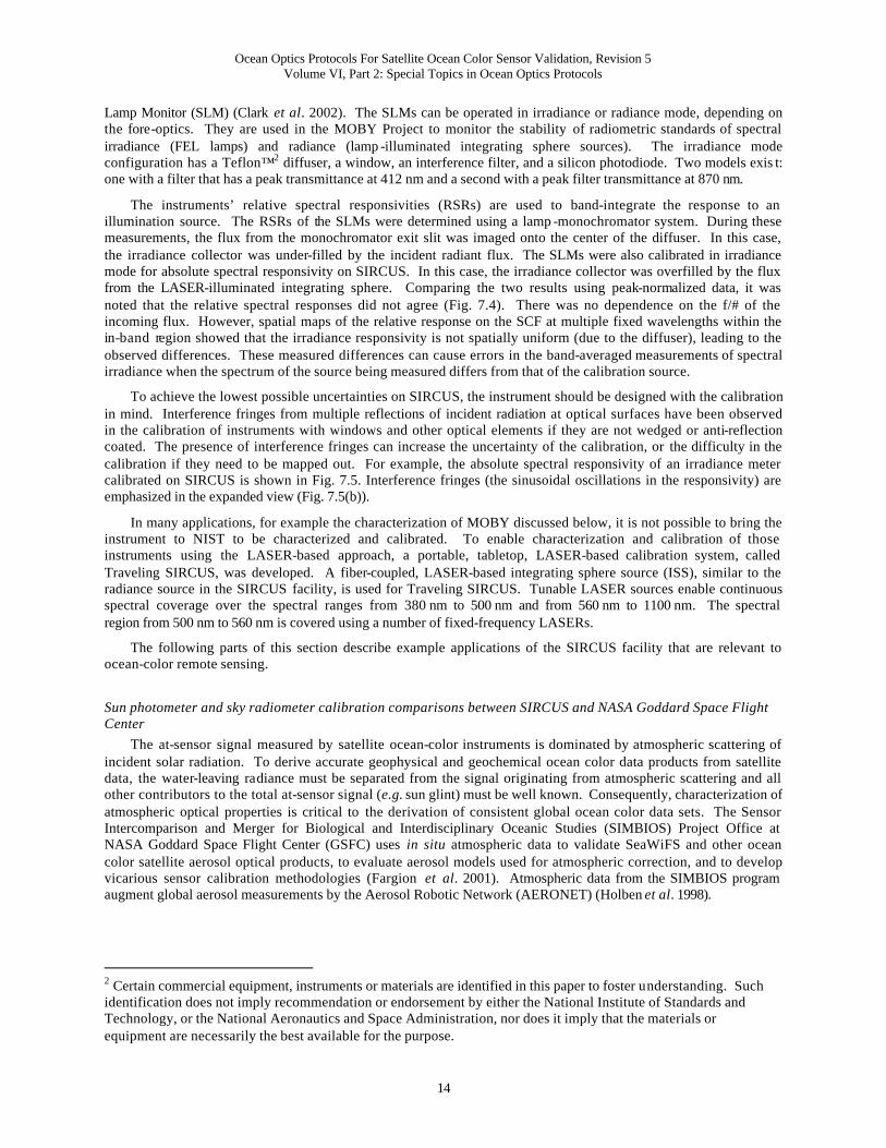
General characteristics of the NIST LASER-based and lamp -based facilities are listed in Table 7.1. Some of the advantages of the LASER-based calibration approach are illustrated by the calibration of the NIST Photo-Electric Pyrometer (PEP) used to radiometrically determine the temperature of a blackbody (Gibson et al. 1998). The instrument is equipped with a narrow bandpass filter (~ 1 nm) for spectral selectivity, making it difficult to study with lamp-illuminated monochromator systems because of their finite spectral bandpass. For accurate radiance temperature determinations, the instrument’s spectral out-of-band responsivity needs to be measured as well. Fig. 7.3 shows the relative spectral responsivity of the PEP determined on SIRCUS, compared with the relative spectral responsivity determined using a conventional lamp -monochromator system in the NIST Spectral Comparator Facility (SCF). As shown in Fig. 7.3(a), the spectral responsivity measured on the SCF is dominated by the spectral bandwidth of the source, and deconvolution of the spectrum using the source slit scatter function is required. In contrast, the fine detail in the spectral responsivity is easily measured on SIRCUS, because of the monochromatic nature of the source. Note that there are several overlying data points at each wavelength along both the rising and falling edges, demonstrating the extreme wavelength stability of the SIRCUS facility. Because of the low flux, the out-of-band responsivity is limited to approximately 10-6 with the lamp -monochromator system (Fig. 7.3(b)). In contrast, the out-of-band responsivity can be measured to the 10-9 level in the SIRCUS facility.

In SIRCUS, instruments are calibrated in their operational state: at the system level, with entrance pupils over-filled. This approach avoids unforeseen errors that can occur using other calibration approaches. For example, consider measurements of the relative spectral responsivity of a single channel filter radiometer known as a Standard

Table 7.1: Comparison of SIRCUS and SCF properties.

Parameter SIRCUS Facility Lamp/Monochromator

Optical Power 300 mW 1 µW

Bandwidth < 0.01 nm 1 nm to 5 nm

Wavelength uncertainty < 0.01 nm 0.1 nm

Power responsivity calibration yes yes

Uncertainty 0.1 % 0.1 %

Irradiance responsivity calibration

yes yes

Uncertainty 0.1 % 0.5 %

Radiance responsivity calibration

yes no

Uncertainty 0.1 %

Digital imaging systems yes no


14

Lamp Monitor (SLM) (Clark et al. 2002). The SLMs can be operated in irradiance or radiance mode, depending on the fore-optics. They are used in the MOBY Project to monitor the stability of radiometric standards of spectral irradiance (FEL lamps) and radiance (lamp -illuminated integrating sphere sources). The irradiance mode configuration has a Teflon™2 diffuser, a window, an interference filter, and a silicon photodiode. Two models exis t: one with a filter that has a peak transmittance at 412 nm and a second with a peak filter transmittance at 870 nm.

The instruments’ relative spectral responsivities (RSRs) are used to band-integrate the response to an illumination source. The RSRs of the SLMs were determined using a lamp -monochromator system. During these measurements, the flux from the monochromator exit slit was imaged onto the center of the diffuser. In this case, the irradiance collector was under-filled by the incident radiant flux. The SLMs were also calibrated in irradiance mode for absolute spectral responsivity on SIRCUS. In this case, the irradiance collector was overfilled by the flux from the LASER-illuminated integrating sphere. Comparing the two results using peak-normalized data, it was noted that the relative spectral responses did not agree (Fig. 7.4). There was no dependence on the f/# of the incoming flux. However, spatial maps of the relative response on the SCF at multiple fixed wavelengths within the in-band region showed that the irradiance responsivity is not spatially uniform (due to the diffuser), leading to the observed differences. These measured differences can cause errors in the band-averaged measurements of spectral irradiance when the spectrum of the source being measured differs from that of the calibration source.

To achieve the lowest possible uncertainties on SIRCUS, the instrument should be designed with the calibration in mind. Interference fringes from multiple reflections of incident radiation at optical surfaces have been observed in the calibration of instruments with windows and other optical elements if they are not wedged or anti-reflection coated. The presence of interference fringes can increase the uncertainty of the calibration, or the difficulty in the calibration if they need to be mapped out. For example, the absolute spectral responsivity of an irradiance meter calibrated on SIRCUS is shown in Fig. 7.5. Interference fringes (the sinusoidal oscillations in the responsivity) are emphasized in the expanded view (Fig. 7.5(b)).

In many applications, for example the characterization of MOBY discussed below, it is not possible to bring the instrument to NIST to be characterized and calibrated. To enable characterization and calibration of those instruments using the LASER-based approach, a portable, tabletop, LASER-based calibration system, called Traveling SIRCUS, was developed. A fiber-coupled, LASER-based integrating sphere source (ISS), similar to the radiance source in the SIRCUS facility, is used for Traveling SIRCUS. Tunable LASER sources enable continuous spectral coverage over the spectral ranges from 380 nm to 500 nm and from 560 nm to 1100 nm. The spectral region from 500 nm to 560 nm is covered using a number of fixed-frequency LASERs.

The following parts of this section describe example applications of the SIRCUS facility that are relevant to ocean-color remote sensing.

Sun photometer and sky radiometer calibration comparisons between SIRCUS and NASA Goddard Space Flight Center

The at-sensor signal measured by satellite ocean-color instruments is dominated by atmospheric scattering of incident solar radiation. To derive accurate geophysical and geochemical ocean color data products from satellite data, the water-leaving radiance must be separated from the signal originating from atmospheric scattering and all other contributors to the total at-sensor signal (e.g. sun glint) must be well known. Consequently, characterization of atmospheric optical properties is critical to the derivation of consistent global ocean color data sets. The Sensor Intercomparison and Merger for Biological and Interdisciplinary Oceanic Studies (SIMBIOS) Project Office at NASA Goddard Space Flight Center (GSFC) uses in situ atmospheric data to validate SeaWiFS and other ocean color satellite aerosol optical products, to evaluate aerosol models used for atmospheric correction, and to develop vicarious sensor calibration methodologies (Fargion et al. 2001). Atmospheric data from the SIMBIOS program augment global aerosol measurements by the Aerosol Robotic Network (AERONET) (Holben et al. 1998).

2 Certain commercial equipment, instruments or materials are identified in this paper to foster understanding. Such identification does not imply recommendation or endorsement by either the National Institute of Standards and Technology, or the National Aeronautics and Space Administration, nor does it imply that the materials or equipment are necessarily the best available for the purpose.


15

Figure 7.3: Comparison of the normalized relative spectral responsivity of the PEP measured on the SCF (top graph) and the SIRCUS (bottom graph); (a) linear and (b) log scale. (Brown and Johnson 2003c)


16

0

0.2

0.4

0.6

0.8

1

830 840 850 860 870 880 890

Wavelength [nm]

Nor

mal

ized

Res

pons

ivity

[a.u

.]SIRCUS

Lamp/Monochromator

Figure 7.4: SIRCUS and SCF (lamp/monochromator) measurements of the spectral responsivity of the 870 nm SLM in irradiance mode. The data have been normalized to the maximu m value.

Figure 7.5: SIRCUS calibration of an irradiance meter showing interference fringes. (a) absolute spectral responsivity of the irradiance meter (b) expanded view of the interference fringes. The solid line is a fit to the data. (Brown and Johnson 2003c)

Sun photometers and sky radiometers are used for atmospheric characterization. Sun photometers are used to determine the atmospheric optical depth while radiance determined from sky radiometers constrains the aerosol models input into radiative transfer codes that calculate the atmospheric contribution to the at-sensor signal. Instruments are calibrated for irradiance responsivity against reference sun photometers using the cross-calibration technique at NASA GSFC (Pietras et al. 2001, 2003). The cross-calibration technique consists of near simultaneous solar observations at GSFC with the uncalibrated instrument and a calibrated reference sun photometer. Reference sun photometers, which are part of the AERONET project, are calibrated using the Langley-Bouger technique at the Mauna Loa Observatory on regular intervals. The method assumes that the ratio of the output voltages for the same


17

channel (e.g., same spectral responsivity) for the reference and uncalibrated radiometers and a particular air mass is proportional to the ratio of the output voltage at zero air mass. If the spectral responsivities differ, a correction is made for spectral differences related to Rayleigh, ozone, and aerosol attenuation. The uncertainty in the calibration at GSFC is approximately 2 %.

Instruments are calibrated for radiance responsivity using a NIST-traceable lamp -illuminated integrating sphere source at NASA GSFC. The primary standard is an FEL standard irradiance lamp. A reference spectroradiometer equipped with an integrating sphere irradiance collector, the OL746/ISIC, is calibrated for irradiance responsivity against the standard irradiance lamp. The irradiance calibration is then transferred to NASA’s “Hardy” sphere using the OL746/ISIC. Knowing the irradiance responsivity of the OL746/ISIC, the distance between the sphere exit port and the entrance aperture to the 746/ISIC, and the sphere exit port area, it is straightforward to calculate the spectral radiance of the “Hardy” sphere. The uncertainty in the radiance responsivity calibration is estimated to be approximately 5 % (k = 2).

Two multi-channel filter radiometers used in the SIMBIOS program were calibrated for irradiance and radiance responsivity on SIRCUS and the results compared with standard calibrations (Souaidia et al. 2003). The Satellite Validation for Marine Biology and Aerosol Determination (SimbadA) radiometers are eleven-channel filter radiometers with bandpasses of approximately 10 nm and center wavelengths at 350 nm, 380 nm, 410 nm, 443 nm, 490 nm, 510 nm, 565 nm, 620 nm, 670 nm, 750 nm and 870 nm, respectively. For comparison to the GSFC sun-photometer cross-calibration results, the SIRCUS-derived irradiance responsivities s(λ) were used to predict a top-of-the-atmosphere (TOA) signal Vo(SIRCUS):

( ) ( ) ( )oV SIRCUS s E d= λ λ λ∫ (7.1)

where s(λ) is the spectral responsivity of one of the radiometer channels and E(λ) is an exo -atmospheric solar irradiance spectrum. Souaidia et al. (2003) used the exo -atmospheric solar irradiance spectra developed by Neckel and Labs (1984), Wehrli (1985), MODTRAN (Berk et al. 1989), and Thuillier et al. (2003). To perform the integration, the s(λ) and the E(λ) were interpolated to a uniform wavelength interval of 0.25 nm and integrated. Results for the 440 nm, 490 nm and 750 nm channels are shown in Table 7.2 (from Souaidia et al. 2003). Predicted results for the 750 nm channel and the 490 nm channel agreed with the cross-calibration to within 2 %; the agreement for the 440 nm channel was approximately 5 %.

Table 7.2: Relative differences [%] between a sun photometer’s TOA signal Vo based on SIRCUS characterization and cross-calibration at GSFC.

(Vo (measured)- Vo (predicted))/Vo(measured) [%]

Channel Center

Wavelength Vo

Measured Neckel and Labs

(1984)

Wehrli

(1986) MODTRAN

(Berk et al. 1989) Thuillier et al.

(2002)

1 443.74 2.3033E+06 5.29 5.44 4.83 4.79 2 493.77 2.9403E+06 1.31 1.46 1.60 0.22 7 752.55 3.3100E+06 1.17 1.33 0.57 0.76

The dominant source of uncertainty in the SIRCUS-based predicted TOA signal was the solar irradiance spectrum used. Changes of 1 % or so were observed, depending on the exo -atmospheric solar irradiance spectrum chosen. Given a cross-calibration uncertainty of ~ 2 %, we are able to validate the cross-calibration with a combined expanded uncertainty (k = 2) of ~ 4 %. The agreement for the 490 nm and 750 nm channels is within the combined uncertainties, but the 440 nm results are not and warrant further investigation.

To compare the two sets of radiance measurements, radiance responsivities, s(λ), were interpolated to a uniform wavelength interval, as were the sphere spectral radiance values, L(λ), for the lamp -illuminated integrating sphere source. The measured signal was then compared to the predicted signal using equation (7.1), but replacing E(λ) with L(λ) and using the instrument’s radiance responsivity instead of its irradiance responsivity. We obtained differences in the calibrations between 2 % and 4 %, depending on wavelength. The radiance responsivity results


18

were consistent with results of an intercomparison performed at NASA GSFC in 2001 (Butler et al. 2002a; Butler et al. 2002b).

As a cross-check, the SimbadA instruments were also calibrated against a NIST-maintained lamp -illuminated integrating sphere source that had been recently calibrated on FASCAL (Walker et al. 1987a). The preliminary results agree with the SIRCUS measurements within approximately 0.5 % with the exception of channel 8, where large interference fringes were observed in the SIRCUS measurements. The results are in agreement with previous comparisons of lamp -based and LASER-based radiance responsivity calibrations of filter radiometers (Johnson et al. 2003). The expanded uncertainty (k = 2) in the radiance responsivity determined on SIRCUS was approximately 0.25 %, a significant reduction from the 5 % uncertainty using the “Hardy” sphere.

Correct description and understanding of aerosols are critical because of their direct and indirect radiative interactions with the atmosphere and their role in atmospheric correction algorithms (http://www.climatescience.gov). Passive remote sensing at discrete wavelengths in networks, such as AERONET, yield values of aerosol optical depth (from down-welling solar irradiance) and information on the phase function, single-scattering albedo, complex index of refraction, and particle size distribution (from the angular distribution of sky radiance). The sensitivity of the derived parameters to the radiometric measurement uncertainty is complicated because of the non-linearity of the retrieval process and the existence of additional effects such as reflected flux from the surface, pointing error, cloud screening, aerosol distributions, model assumptions, etc. The sensitivity analysis of Dubovik et al. (2000) assumed a wavelength independent uncertainty in total optical depth of 0.01 and an uncertainty in the sky radiance values of 5 %, based on AERONET. They found these uncertainties to be inadequate for the case of low optical depths, a situation that can occur over oceans (Dubovik et al. 2000). In a separate study involving satellite measurements over the ocean, differences of only a few tenths of a percent in the radiometric calibration compromised the accuracy of the aerosol optical depth determinations (Mishchenko et al. 1999).

Laboratory calibration of sun photometers is important for independent assessment of their stability as well as to assess the uncertainties and validity of the exo -atmospheric solar irradiance measurements (Schmid et al. 1998). Detailed characterization and calibration of primary sun photometers using SIRCUS, and other primary standard calibration facilities, would produce additional comparison data and quantify other sources of error such as exact mapping of the field-of-view (important because of scattering within the baffle tube) and the temperature dependence of the radiometric responsivities (important because ambient temperature varies dramatically during field use).

Stray light characterization and correction of spectrographs Detector array-based spectral imaging systems, such as spectrographs, enable the simultaneous acquisition of an

entire spectrum over some finite spectral region of interest; they can acquire a spectral image in a matter of seconds. The ability to rapidly acquire a full spectrum has led to the use of array-based systems in a variety of ocean color applications where the source may not be stable over minutes. Spectrographs commonly consist of an entrance port, a dispersing element (such as a grating) to spatially resolve the spectral components of the incident radiation, and mirrors to image the entrance port (often a slit) onto a detector reference plane. Because of the dispersing element, the spatial image of the entrance port falls on different regions of the detector array, depending on its wavelength; broadband sources form an image across the entire array. The spectral coverage of a spectrograph is determined by the size of its detector array, the dispersion properties of its grating, and its optical layout.

Two CCD-spectrographs, one for the blue spectral region (360 nm to 640 nm), referred to as the BSG, and another for the red (560 nm to 940 nm), the RSG, form the basis of the Marine Optical System (MOS), the sensor used in MOBY (Clark et al. 2003). The same dual-spectrograph design is used for the MOS Profiler, a ship-board-deployable version of the MOBY sensor used in the development of bio-optical algorithms. The response of the two MOS spectrographs to monochromatic LASER excitation is shown in Fig. 7.6. The spectra are similar for both spectrographs. There are four components to the image: a strong sharp peak corresponding to the image of the spectrograph entrance slit on the CCD; a broad, peaked structure around the slit image; a non-zero constant component, and an additional peak. The first three components are similar to specular, haze, and diffuse components of reflectance, respectively. They remain approximately invariant as the excitation wavelength is changed and the image moves across the CCD array. From physical examination of the spectrographs, the fourth component (the additional peak) arises from a spurious reflection off a mirror coupled with higher-order diffraction from the grating. As the image moves across the array, the reflection peak changes size, shape and position with


19

respect to the primary peak. The specular component corresponds to the properly imaged radiation; the other components arise from light scattered in the spectrograph, principally from the grating. The ‘specular’ component in the spectrograph image is analogous to the ‘in-band’ component of a filter radiometer’s responsivity, while the sum of the other three components is analogous to the ‘out-of-band’ component.

Figure 7.6: MOS response to monochromatic excitation at (a) 550 nm (for the blue spectrograph) and (b) 700 nm (for the red spectrograph).

This unwanted background radiation, while small, is fairly typical for single grating spectrographs and can give rise to unforeseen errors, often much larger than anticipated, when the spectral distribution of a source being measured differs significantly from that the calibration source. Such a situation is routinely encountered in ocean color measurements, where instruments are calibrated against incandescent sources having peak radiances in the near infrared and subsequently measure the optical properties of the ocean, where the upwelled radiance peaks in the blue to green spectral region. Consequently, to fully understand the radiometric performance of a spectrograph used for ocean color measurements, it is important to characterize the stray light in the system.

Knowing the relationship between the excitation wavelength and the position of the image on the array enables us to determine the fraction of incident light at some wavelength that is scattered onto a particular element. For example, for the wavelength λex in Fig. 7.6(top), 0.01 % of the light imaged on element 190 (BSG) is scattered onto element 300. Assuming each element in the detector array has the same average spectral responsivity, the signal from element 300 to radiation at wavelength λex is 0.01 % of the signal from element 190.

A single image, however, does not give us the spectral resolution required to determine a pixel’s in-band relative spectral response. For this information, it is necessary to tune the monochromatic excitation source in fine steps, a situation SIRCUS is well equipped to address. Figure 7.7 shows the relative spectral responsivity of adjacent pixels of the MOS RSG detector array as the LASER excitation wavelength on SIRCUS is tuned over the range from 587 nm to 593 nm in 0.1 nm steps. At each excitation wavelength, the responsivity of each pixel is separately determined. By tuning the excitation wavelength over a broad spectral range, a single pixel’s absolute spectral responsivity (and slit scatter function (Kostkowski 1997)) can be determined. A pixel’s slit scatter function image is similar to but different from a single image. In Fig. 7.8, an image acquired at a pixel’s peak responsivity is plotted along with the slit scatter function. While the ‘haze’ and ‘diffuse’ components are similar, note the


20

reflection of the second peak about the primary image and the narrowing of its width in the slit scatter function compared with the single image.

Knowing the slit-scatter function, we have a set of coupled equations equal to the number of elements in the array:

( ) ( ) ( )i i i i iS r L d= λ σ λ − λ λ λ∫ . (7.2)

Si is the signal from pixel i; ( )i ir λ is that array element’s peak responsivity; ( )i iσ λ − λ is element i’s slit scatter

function; and ( )L λ is the spectral radiance of the source being measured. Equation (7.2) can be directly solved for

either ( )i ir λ or ( )L λ , provided the other variable is known. Utilizing the discrete nature of arrays, and relating

each array element to a band-center wavelength, an iterative approach has been used to correct MOS instruments located in MOBY and the MOS Profiler (Brown et al. 2003b). A matrix-based approach is currently being developed (see below) to determine each element’s responsivity and to subsequently determine the spectral radiance of an unknown source (e.g. upwelling radiance in the ocean).

Figure 7.7: Spectral responsivity of pixels 428 to 432 (from left to right).

Figure 7.8: A pixel’s slit scatter function (SSF) and an image acquired with an excitation wavelength tuned to the peak response of the pixel.


21

Least-squares matrix solutions for spectrograph stray light characterization

In this subsection we describe a generalized least-squares approach to deconvolution as an alternative to the iterative procedure currently used to correct spectrographs for stray light (Brown et al. 2003b). The method is simpler to apply than the iterative approach, faster to run, and does not require empirical separation of in-band and out-of-band regions of a channel’s spectral responsivity.

The signal iS at the ith spectrograph detector element, when viewing a source of spectral radiance ( )L λ , is

( ) ( ) ( ) ( ) ( )0 0

,i i i i i iS r L d r L d∞ ∞

= λ λ λ λ = λ σ λ − λ λ λ∫ ∫ , (7.3)

where ( )ir λ is the element’s spectral responsivity, ( )i ir λ is its peak responsivity at the characteristic wavelength

iλ of the detector element, and ( )i iσ λ − λ is the normalized spectral responsivity function. The normalized

spectral responsivity function may be expressed as the sum

( ) ( )0

N

i i in in=

σ λ − λ = σ λ −λ∑ , (7.4)

where ( )0i iσ λ −λ is the spectrograph’s in-band slit response function and ( ), 1, ,in i n Nσ λ −λ = … are (out-of-band) stray light response functions describing the wavelength dispersions associated with N distinct stray light processes.

Assuming that the discrete detector elements are spaced in the slit dispersion image at a uniform interval ∆λ , the discrete spectral radiance associated with each detector may be expressed

( )2

2

1 i

i

iL L dλ+∆λ

λ−∆λ

= λ λ∆λ ∫ (7.5)

and the composite normalized spectral responsivity function becomes

( ) ( )2

0 2

1, , 1, ,512

j

j

N

ij i j in in

d i jλ − ∆ λ

= λ − ∆ λ

σ λ − λ = σ λ − λ λ =∆λ ∑ ∫ … . (7.6)

Note that each element in the detector array is assumed to have the same spectral responsivity.

We may express (7.3) in discrete form as

( ) ( )512

1i j j i j j

j

S r L=

= λ σ λ − λ ∆λ∑ , (7.7)

introduce the integrated in-band responsivity

( ) ( ) ( )00

i i i i i iR r d∞

λ ≡ λ σ λ − λ λ∫ . (7.8)

and assume that the in-band slit function is constant for all detector elements.

Substituting from (7.8), (7.7) becomes in general form

( )( ) ( )

512

10

0

1i j j i j i j j

ji i

S R Ld

∞=

= λ σ λ − λ ∆λσ λ − λ λ

∑∫

. (7.9)

It is convenient to define


22

( )( )0

0

ˆ i j i ji j

i i d∞

σ λ − λσ =

σ λ − λ λ∫, (7.10)

and express equations (7.9) in matrix form as

( ) ( )S D R L D L Rv v v v v% % = Σ = Σ , (7.11)

where the elements of the matrix S% are ˆ ijσ and the elements of vectors Sv

, Rv

and Lv

are the radiances Si,

responsivities Rj and radiances Lj, respectively. The matrices ( ) D Lv

and ( ) D Rv

have the elements of the

vectors Lv

and Rv

, respectively, on the main diagonal, and are zero elsewhere. The first form of the right-hand-side of (7.11) is used to determine the radiance spectrum when the responsivity vector is known, and the second form of the right-hand-side of (7.11) is used with instrument calibration data to determine responsivity from known radiances.

To calibrate the spectrograph responsivities after viewing a calibration source with known radiances CLv

and

recording response signals CSv

, we form the product matrix

( )CD Lv% % Γ = Σ , (7.12)

substitute in (7.11) and multiply both sides by T%Γ to obtain

T TCS R

v v% % % Γ = Γ Γ , (7.13)

yielding the formal least-squares solution for responsivity

1-T T

CR Svv % % % = Γ Γ Γ . (7.14)

Given now the responsivity vector Rv

from that calibration, we form the product matrix

( )D Rv% % Λ = Σ , (7.15)

substitute in (7.11) and multiply both sides by T%Λ to write

T TS Lv v% % % Λ = Λ Λ . (7.16)

We define the system inverse responsivity matrix as

1T T% % %% −

Ζ = Λ Λ Λ , (7.17)

and write the solution to (7.16) as

L Svv %= Ζ . (7.18)

Equations (7.13) and (7.16) are the normal equations for the unconstrained least squares solutions (7.14) and (7.18) for R

v and L

v, respectively (Press et al. 1997). The pair of solutions requires determination of the inverses of

the two square, symmetric matrices T% % Γ Γ and T% % Λ Λ . Programs are available in most numerical analysis

packages, such as MATLAB, to determine the inverse of a square, symmetric matrix using a variety of direct inversion algorithms. Since the number of unknowns (N) equals the number of equations (N), this would seem the obvious method of solution. Unfortunately, with real data containing noise, the system of equations may become degenerate. In such cases, the direct inversion algorithms may either fail altogether, or yield unstable and unreasonable solutions. A better approach is to decompose each matrix T% % Γ Γ and T% % Λ Λ into its singular values

, 1,2, ,jw i N= … , and associated left and right singular vectors using Singular Value Decomposition (SVD), and

determine its approximate inverse (Press et al. 1997).

Any matrix with M rows and N columns can be written as the product

,= TA UWV% % % % (7.19)


23

where W% is the diagonal matrix of singular values 0jw ≥

1

2

0 0

0.

0

0 0 N

w

w

w

=

W

LO M%

M O OL

(7.20)

and U V% % are matrices containing left and right singular column vectors, respectively, each of which is associated with the corresponding singular value. These matrices are orthonormal in the sense that

,= =T TU U V V I% % % % % (7.21)

where I% is the identity matrix, i.e. the transpose of each matrix is its inverse.

If the matrix A% is square (as in the present case) and not degenerate (i.e. as might result from measurement noise – resulting in an underdetermined system of equations) then there will be N significant singular values. If M < N, or the matrix is degenerate, there will be less than N significant singular values. In any event, by arranging the singular values in decreasing order, when one becomes too small, we can truncate the matrix at some K N≤ and still proceed with an approximate solution. For a direct solution, it minimizes the length of the residual, and if the matrix equation is cast into least-squares context, the SVD solution is the approximate solution with the minimum squared residuals.

Finally for a square matrix A% , its inverse may be determined (or approximated in an optimal way if K N≤ ) from its SVD decomposition as

1 1 ,− −= TA VW U% % % % (7.22) where

11

121

1

0 0

0.

0

0 0 K

w

w

w

−

−

−

−

=

W

LO M%

M O OL

Stray light corrections to MOBY upwelled radiance measurements using different slit response function models

It is of interest to compare the matrix solution for MOBY stray light responsivities and stray light corrected, upwelled radiance measurements using the approximate in-band slit response function underlying the iterative recursion solution (Brown et al. 2003b), and the solution obtained using a more realistic approximation to the slit response function.

To obtain the recursion relationships in current use for MOBY data, it is necessary to use (7.4) to express (7.9) in the form

( ) ( )

( )

( ) ( )

( )

512 512

01 1 1

0 00 0

N

j j i j i j j j j ijn i j jj j n

i

i i i i

R L R LS

d d

= = =∞ ∞

λ σ λ − λ ∆λ λ σ λ − λ ∆λ= +

σ λ − λ λ σ λ − λ λ

∑ ∑ ∑

∫ ∫, (7.23)

which separates the in-band response from the net out-of-band response. We then assume

( ) ( ) constantj j j i i iR L R Lλ ≈ λ ≈ over the very narrow non-zero range of ( )0i iσ λ −λ , and since by definition

( ) ( )512

0 01 0

i j i j i ij

d∞

=

σ λ − λ ∆ λ = σ λ − λ λ∑ ∫ , equation (7.23) is reduced to


24

( )( ) ( )

( )

512

1 1

00

N

j j ijn i j jj n

i i i i

i i

R LS R L

d

= =∞

λ σ λ − λ ∆λ= λ +

σ λ − λ λ

∑ ∑

∫. (7.24)

In the approximation represented by (7.24), the contributions from all detector pixels in the in-band range are combined to form a delta function ˆ 1i iσ = , and the combined in-band and out of band spectral response

characteristics are expressed in the matrix %Σ as

( )

( )1

00

1,

ˆ 0, 9,

, 9

i j

N

ijn i jn

i i

j i

i j j i

i jd

=∞

=σ = − ≤ ≠ σ λ − λ ∆λ

− > σ λ − λ λ

∑

∫

. (7.25)

Alternatively we may assume a Gaussian model of the in-band slit response function, which for the BSG is

( )2

0

1 00.001+exp ,

2 0.395i i

Pix Pix − σ λ −λ ≅ − (7.26)

and add it to the out-of-band function ( )1

N

in in=

σ λ −λ∑ (the sum of the N stray light mechanisms), substitute the sum

in (7.6) and integrate it over the bandwidth of each pixel to determine the elements ˆ ijσ of the matrix %Σ . The in-

band segment of the continuous and discrete representations of ˆ ijσ are illustrated in Figure 7.9.

The stray-light corrected responsivities computed using the delta function and Gaussian function in-band models are compared, in Figure 7.10, to the responsivities that are not corrected for stray light (system output divided by source radiance) for one radiometric calibration of a MOBY BSG Lu configuration. The two stray-light responsivity solutions are identical except at the boundary where the second-order reflection “bump” in the out-of-band stray light function enters and leaves the extent of the in-band slit function (Brown et al. 2003b), and at the endpoints. These sharp discontinuities in the responsivity interact with the relatively coarse discrete representation of (7.26) (see Fig. 7.9) and result in overshoot signatures. An example of the uncorrected and stray-light corrected (delta-function in-band) responsivity calibrations of one MOBY upwelled radiance measurement are compared in Fig. 7.11 to illustrate the magnitude and spectral quality of the correction. The corresponding stray-light corrected calibration of this upwelled radiance spectrum (not shown) is equivalent in magnitude and structure to that shown in Fig. 7.11, but tends to overshoot in the sharp Fraunhofer line features of the measured spectrum. Essentially, this “more correct” representation is “trying too hard” to match this highly structured spectrum. The next step to obtain an optimal balance between the unconstrained solution using (7.26) and the relatively crude delta-function solution (7.25) is to constrain the least-squares solution using the method of Twomey (1977), which is described also by Schumaker (1979) and Press et al. (1997).


25

0.0

0.1

0.2

0.3

0.4

0.5

0.6

0.7

0.8

0.9

1.0

-10 -8 -6 -4 -2 0 2 4 6 8 10

Pixel Offset

Rel

ativ

e R

espo

nsiv

ity

Figure 7.9: Gauss in-band slit response function (thin gray line), and in-pixel-bandwidth averages obtained by integrating the function over each pixel bandwidth (thick black line).

0

10

20

30

40

50

60

70

80

90

100

0 100 200 300 400 500

Pixel Number

Rad

ianc

e R

espo

nsiv

ity

Figure 7.10: Radiance responsivities of a MOBY MOS. The top curve is the responsivity obtained by dividing the sensor output by the calibration source spectral radiance without stray light correction, and the bottom two dashed curves represent the stray light corrected responsivities using the delta-function in-band response model (darker dashes) and the Gaussian model of the in-band slit response function (gray dashes). The two stray light corrected responsivities are distinguishable only by the overshoot of the Gaussian model result near the end-points and near pixels 220 and 260.


26

0

0.2

0.4

0.6

0.8

1

1.2

1.4

0 100 200 300 400 500 600

Pixel

Upw

elle

d R

adia

nce

( µW

cm

-2 n

m-1

sr-1

)Uncorrected Lu

SLC Lu (delta fct slitresponse model)

Figure 7.11: An example comparison between a calibration not corrected for stray-light (solid line) and a stray-light corrected (SLC) calibration (dashed line) of a MOBY upwelled radiance measurement during a deployment. The stray light correction shown is based on the delta-function approximation of the MOS spectrograph in-band response function (see text).

Stray light, ocean color and bio-optical algorithms As discussed in detail by Brown et al. (2003b), MOBY’s system response has been corrected for stray light.

MOBY is used for the vicarious calibration of a number of ocean color satellites and any changes in MOBY-derived water-leaving radiances are directly reflected in satellite sensor calibration coefficients for the relevant channels. Consider the impact on MODIS as a representative example of the impact of the stray light correction of MOBY. MODIS bands 8 through 12 (412 nm to 551 nm) are vicariously calibrated against MOBY. The stray-light-correction factors for MOBY (the correction factors are simply the ratio of the stray-light-corrected to the uncorrected measurements) in terms of ( )WNL λ at the MODIS band-averaged wavelengths over 5 years of

deployments are given in Fig. 7.12. Each left-to-right grouping in the figure is a separate buoy deployment. Note that two different Marine Optical System (MOS) spectrograph systems are used: one for even numbered buoy deployments and another one for odd numbered buoy deployments. The correction factors range from + 8 % for Band 8 to –2.5 % for Bands 11 and 12. There are slight differences in the stray light corrections for the two different MOS systems. There was an increase in the magnitude of the stray light correction factor for Band 8 for 3 Buoy deployments around 1999. During these deployments, a different optical fiber was used. With the exception of these Buoys, the correction factors have been stable over the entire deployment sequence, implying that the MOBY imaging and the MOS slit-scatter functions, along with the ocean-color measurements, have remained stable over this time frame. The observed radiometric stability of the MOBY systems (Barnes et al. 2000;Clark et al. 2003; Brown et al. 2003b) enables us to correct previous deployments for stray light with confidence.


27

Figure 7.12: MOBY LWN stray light correction factors for MODIS bands.

The stray light corrections to the MODIS sensor channel calibrations are constant (systematic), and should they not be applied, significant errors will occur in relevant data products. For example, the Band 9 to Band 12 ratio is used to derive chlorophyll-a concentration. The effect of using stray light corrected MOBY LWN(λ) for vicarious calibration of MODIS, increases the MODIS Band 9 responsivity by 3 % and decreases the Band 12 responsivity by approximately 2.5 %. Correspondingly, the measured at-sensor radiance decreases by 3 % in Band 9 and increases by 2.5 % in Band 12, leading to a total decrease of ~ 5 % in the Band 9 to Band 12 ratio. The error arising in the chlorophyll a concentration as a function of the MODIS total-band Band 9 to Band 12 ratio is shown in Fig. 7.13 for systematic errors of 1 %, 5 %, and 10 %. Correcting the MODIS sensor calibration for stray light in MOBY eliminated a systematic error that ranged from 15 % for green water (low ratios of Band 9 to Band 12) to almost 50 % for bluest waters (high ratios of Band 9 to Band 12).


28

-100

-80

-60

-40

-20

0

20

40

60

80

100

-0.5 -0.3 -0.1 0.1 0.3 0.5 0.7 0.9 1.1

Log of MODIS Total Band Lwsn 09/12 Ratio

% D

iffe

renc

e in

Par

amet

er 1

3,

CZ

CS_

pigm

ent (

%)

-10 %

-5 %

5 %

10 %

-1 %

1 %

Figure 7.13: The relationship between MODIS band ratios and chlorophyll-a concentration.

Figure 7.14: a) The sensitivity of the bio-optical algorithm to changes in band ratio with SLC (black line), compared to without SLC (grey line). The arrow identifies a pair of SLC corrected (black diamond) and uncorrected (gray diamond) versions of a single data point (LWN ratio and chlorophyll a concentration). b) An expanded view of the fit to data from oligotrophic waters.

Of course, it is mis leading to only consider the effect of stray light on the vicarious calibration to derived data products. In general, all systems used in the development of remote sensing ocean color data products should be characterized and corrected for stray light, including systems used in the development of bio-optical algorithms. A shipboard deployable version of the MOBY sensor known as the MOS Profiler is used in the development of MODIS bio-optical algorithms. It has been characterized for stray light and a correction algorithm was developed


29

for it as well (Brown et al. 2003a). The effect of stray light correction of the MOS Profiler on MODIS “total band” chlorophyll a bio-optical algorithm is shown in Fig. 7.14. The solid gray line represents the chlorophyll a bio-optical algorithm without stray light correction, while the solid black line represents the algorithm with stray light correction of MOS. Note that the stray light correction increases the chlorophyll concentration as a function of band ratio – in particular for blue water. The arrow in the figure points to the effect of stray light on the measured ratio. The open triangle is uncorrected for stray-light, while the solid triangle to the right is the same data with the stray light correction applied.

Because similar MOS instruments are used in MOBY and in the MOS Profiler, the stray light correction is similar for both instruments. Consequently, the changes in band ratios as measured by MOBY, upon application of the stray light correction algorithm are compensated by the changes in the bio-optical algorithm derived from MOS Profiler measurements in MOBY waters. This is expected, because the measured chlorophyll concentration did not change. So the stray light correction to the bio-optical algorithm results in an increase in chlorophyll a concentration determined as a function of MODIS band ratios for low chlorophyll waters. Figure 7.15 shows chlorophyll a concentration in the Hawaiian islands before the stray light correction to the bio-optical algorithm (left) and after the stray light correction is applied (right). The darker regions in the right hand figure, with respect to the left hand figure, represents increases in derived chlorophyll-a concentrations.

As has been shown above for stray light, small systematic errors in radiometric measurements can add significant error to the resultant data products in ocean-color remote sensing. For reliable, long-time-series, global ocean color measurements, all instruments involved in radiometric measurements, including satellite sensors, vicarious calibration sensors, and sensors used in the development of bio-optical algorithms and atmospheric characterization need to be fully characterized (and usually corrected) for systematic errors, including not only stray light but other sources of systematic error such as temperature and wavelength.

Figure 7.15: Chlorophyll-a concentrations (log scale) in the Hawaiian islands before (a) and after (b) stray light correction of the bio-optical algorithm.

7.4 LUNAR RADIOMETRY A NASA-sponsored facility for radiometric characterization of the Moon has been developed to enable on-orbit

calibration of remote sensing imaging instruments (see www.moon-cal.org). The RObotic Lunar Observatory (ROLO), located at the Unites States Geological Survey (USGS) facility in Flagstaff, Arizona, has demonstrated the capability to assess post-launch instrument response trends with accuracies approaching 0.1 % (Kieffer et al. 2003). Using the Moon as an on-orbit radiometric source eliminates sources of uncertainty in ground-based vicarious calibrations arising from atmospheric scattering of incident and reflected solar radiation, but requires a spacecraft attitude maneuver for nadir-viewing instruments. Although the radiometric properties of the lunar surface are extremely stable [< 10-8 yr-1 (Kieffer 1997)], the radiance of the lunar disk depends in complex ways on the angles of illumination and viewing. Therefore, on-orbit calibrations based directly on comparisons between successive


30

observations of the Moon are not practical; instead on-orbit comparisons using the Moon are realized through use of a photometric model developed by the USGS lunar science team.

The ROLO project has developed a spectral radiometric model of the Moon capable of predicting the disk-integrated lunar irradiance at a specified time and location corresponding to a spacecraft instrument observation. Lunar irradiance varies significantly with absolute phase (a factor of 10 between quarter and full moon), and libration angles (~ 5 % over the range seen by a ground-based observer). Consequently, the model input data for fitting a photometric function requires a wide range of geometric coverage. ROLO has amassed a more than five-year collection of ground-based telescope observations of the Moon, covering phase angles up to 90o and the full range of libration angles seen from Flagstaff, Arizona. The Moon is imaged in 23 visible and near-infrared (VNIR) bands, seven of which coincide with MODIS wavelengths, and 9 short-wave infrared (SWIR) bands. The spatially-resolved lunar images are calibrated to exo -atmospheric radiance and integrated to disk-equivalent irradiance; these values constitute the input data for the ROLO irradiance model. The analytic form of the model has been developed empirically, based on reduction of residuals in the fitting process. The mean absolute residual of the fit is 0.96 %; however, this value is a measure of the internal consistency of the model, and does not reflect the accuracy of the absolute radiometric scale, which currently is being evaluated.

SeaWiFS has incorporated lunar calibration into their system radiometric response definition, and has used lunar irradiance comparisons to assess and correct sensor degradation trends (Barnes et al. 2001). SeaWiFS has made regular observations of the Moon since November 1997, consistently at a phase angle near 7 degrees. To view the Moon, the spacecraft executes a pitch maneuver as it enters the Earth's shadow after passing the South Pole. The normally nadir-locked pitch rate is reversed, and the instrument scans past the Moon as the spacecraft passes the sub-lunar point on the orbital ground track. At the end of the maneuver, when the instrument again points toward the Earth, the pitch rate is returned to normal. This maneuver is conducted once every month, approximately.

The SeaWiFS observations of the Moon have been compared with the ROLO lunar irradiance model using an established protocol for spacecraft instrument team interaction with ROLO (see www.moon-cal.org). In brief, the instrument team provides to ROLO their instrument’s relative spectral response and spatial resolution (one time only), and for each lunar observation: the UTC and spacecraft location in J2000 coordinates, the down-track size of the lunar image in the instrument field-of-view (FOV), and the measured lunar irradiance calculated using the usual instrument radiance calibration. The ROLO team generates the ephemeris for the Sun and Moon at the time of the observation, calculates all geometric angles and distance corrections, interrogates the lunar model for the specified geometry, and reports the discrepancy with the instrument team's measure of irradiance.

Comparisons of the first 50 SeaWiFS lunar observations to the ROLO model showed responsivity drifts of approximately 4 % in band 7 (766 nm) and 10 % in band 8 (866 nm), while bands 1 through 6 remained essentially stable. Based on these results, the SeaWiFS Project has developed asymptotic, time-dependent corrections for their ocean color radiances (Barnes et al. 2001). Figure 7.16(a) shows the direct comparisons of SeaWiFS with lunar irradiance for the first 70 observations. The band-correlated temporal jitter seen in these time series probably arises from uncertainty in the spatial sampling used for the irradiance computations, due to the small size of the lunar image on the SeaWiFS focal plane array - approximately 6 x 24 pixels. Figure 7.16(b) shows the result of removing the jitter (averaged over bands 1 through 6) and Fig. 7.17 shows the results of applying the time-dependent corrections now incorporated into SeaWiFS standard data products. The spectral distribution of the plots reflects the current uncertainty in the ROLO model absolute radiometric scale. However, the temporal behavior of these comparison data have established instrument response trending for SeaWiFS with a precision of about 0.1 % per year (Kieffer et al. 2003).

For the ocean, the water-leaving radiance is small in the near-infrared (NIR), allowing for the determination of atmospheric scattering contribution to the at-sensor signal (Siegel et al. 2000), which allows use of radiances in these channels to account for effects of aerosols in the atmospheric correction algorithms for visible wavelengths. Near-infrared channels of ocean color satellite sensors cannot be calibrated vicariously using radiometric buoys stationed in the ocean (e.g. MOBY): the Moon, or land reflectance targets, provide the only possibility for vicarious determination of drifts in a sensor’s responsivity at these wavelengths. Uncorrected, the large responsivity drifts in SeaWiFS Bands 7 and 8 (NIR bands), could compromise the atmospheric correction to ocean color measurements, leading to significant biases and errors in ocean color data products.


31

Figure 7.16: Lunar trending of SeaWiFS bands (a) not corrected for band-correlated jitter, and (b) with band-correlated jitter removed.

Figure 7.17: Corrected temporal relative responsivity of SeaWiFS derived from lunar observations.


32

7.5. SUMMARY We have presented a number of recent developments in radiometry that directly impact the uncertainties

achievable in ocean-color research. Specifically, a new (2000) U. S. national irradiance scale, a new LASER-based facility for irradiance and radiance responsivity calibrations, and applications of the LASER facility for the calibration of sun photometers and characterization of spectrographs were discussed. For meaningful long-time-series global chlorophyll-a measurements, all instruments involved in radiometric measurements, including satellite sensors, vicarious calibration sensors, sensors used in the development of bio-optical algorithms and atmospheric characterization need to be fully characterized and corrected for systematic errors, including, but not limited to, stray light. A unique, solid-state calibration source is under development to reduce the radiometric uncertainties in ocean color instruments, in particular below 400 nm. Lunar measurements for trending of on-orbit sensor channel degradation were described. Unprecedented assessments, within 0.1 %, of temporal stability and drift in a satellite sensor’s radiance responsivity are achievable with this approach. These developments advance the field of ocean color closer to the desired goal of reducing the uncertainty in the fundamental radiometry to a small component of the overall uncertainty in the derivation of remotely sensed ocean-color data products such as chlorophyll a.

ACKNOWLEDGEMENTS The authors gratefully acknowledge support for this work by the U.S. Air Force Metrology, NOAA, and

NASA’s SeaWiFS, MODIS, SIMBIOS, and EOS Calibration/Validation program offices.

REFERENCES Barnes, R. A., R. E. Eplee, Jr., W. D. Robinson, G. M. Schmidt, F. S. Patt, S. W. Bailey, M. Wang and C. R.

McClain, 2000: The calibration of SeaWiFS on orbit, Proceedings of the SPIE, 4135: 281-293.

Barnes, R. A., R. E. Eplee, G. M. Schmidt, F. S. Patt and C. R. McClain, 2001: The Calibration of SeaWiFS. Part I: Direct Techniques, Applied Optics, 40: 6682-6700.

Berk, A., L. S. Bernstein, D. C. Robertson, 1989: MODTRAN: A Moderate Resolution Model for LOWTRAN 7, GLTR-89-0122.

Brown, S. W., G. P. Eppeldauer and K. R. Lykke, 2000: NIST facility for Spectral Irradiance and Radiance Responsivity Calibrations with Uniform Sources, Metrologia, 37: 579-582.

Brown, S. W. and B. C. Johnson, 2003: Advances in radiometry for ocean color, Proceedings of the SPIE, 5151: 441-453.

Brown, S. W., B. C. Johnson, M. E. Feinholz, M. A. Yarbrough, S. J. Flora, K. R. Lykke and D. K. Clark, 2003a: Stray light correction algorithm for spectrographs, Metrologia, 40: S81-S84.

Brown, S. W., B. C. Johnson, S. J. Flora, M. E. Feinholz, M. A. Yarbrough, R. A. Barnes, Y. S. Kim, K. R. Lykke and D. K. Clark, 2003b: Stray light correction of the Marine Optical Buoy. Chapter 5 in: Mueller, J.L., G.S. Fargion and C.R. McClain [Eds.], Ocean Optics Protocols for Satellite Ocean Color Sensor Validation, Revision 4, Volume VI: Special Topics in Ocean Optics Protocols and Appendices. NASA/TM-2003-211621/Rev4-Vol.VI, NASA Goddard Space Flight Center, Greenbelt, MD, pp87-124.

Butler, J. J., B. C. Johnson and R. A. Barnes, 2002a: Radiometric measurement comparisons at NASA Goddard Space Flight Center: Part I. The GSFC sphere sources, The Earth Observer, 14(3): 3-8.

Butler, J. J., B. C. Johnson and R. A. Barnes, 2002b: Radiometric measurement comparisons at NASA Goddard Space Flight Center: Part II. Irradiance lamp comparisons and the NIST sphere source, The Earth Observer, 14(4): 25-29.

Clark, D. K., M. E. Feinholz, M. A. Yarbrough, B. C. Johnson, S. W. Brown, Y. S. Kim and R. A. Barnes, 2002a: An overview of the radiometric calibration of MOBY. Earth Observing Systems VI. W. L. Barnes [Ed.]. Bellingham, WA, Society of Photo-Optical Instrumentation Engineers. 4483: 64-76.


33

Clark, D. K., M. A. Yarbrough, M. E. Feinholz, S. Flora, W. Broenkow, Y. S. Kim, B. C. Johnson, S. W. Brown, M. Yuen and J. L. Mueller, 2003: MOBY, a radiometric buoy for performance monitoring and vicarious calibration of satellite ocean color sensors: measurement and data analysis protocols. Chapter 2 in: Mueller, J.L., G.S. Fargion and C.R. McClain [Eds.], Ocean Optics Protocols for Satellite Ocean Color Sensor Validation, Revision 4, Volume VI: Special Topics in Ocean Optics Protocols and Appendices. NASA/TM-2003-211621/Rev4-Vol.VI, NASA Goddard Space Flight Center, Greenbelt, MD, pp3-34.

Dubovik, O., A. Smirnov, B. N. Holben, M. D. King, Y. J. Kaufman, T. F. Eck and I. Slutsker, 2000: Accuracy assessments of aerosol optical properties retrieved from Aerosol Robotic Network (AERONET) sun and sky radiance measurements, J. Geophys. Res., 105: 9791-9806.

Eppeldauer, G. P., S. W. Brown, T. C. Larason, M. Racz and K. R. Lykke, 2000: Realization of a spectral radiance responsivity scale with a LASER-based source and Si radiance meters, Metrologia, 37: 531-534.

Eppeldauer, G. P. and D. C. Lynch, 2000: Opto-mechanical and electronic design of a tunnel-trap Si- radiometer, J. Res. NIST, 105(6): 813-828.

Fargion, G. S., R. A. Barnes and C. R. McClain, [Eds.], 2001: In Situ Aerosol Optical Thickness Collected by the SIMBIOS Program (1997-2000): Protocols and Data QC and Analysis, NASA/TM-2001-209982, NASA Goddard Space Flight Center, Greenbelt, MD, 103pp.

Fowler, J. and M. Litorja, 2003: Geometric area measurements of circular apertures for radiometry at NIST, Metrologia, 40: S9-S12.

Gibson, C. E., B. K. Tsai and A. C. Parr, 1998: Radiance Temperature Calibrations, NIST Special Publ. 250-43, U.S. Dept. of Commerce, Gaithersburg, MD, 56pp plus Appendices.

Gordon H. R., 1987: Calibration requirements and methodology for remote sensors viewing the ocean in the visible. Remote Sens. Environ., 22: 103-126

Gordon, H. R., 1998: In-orbit calibration strategy for ocean color sensors, Remote Sensing of Environment, 63: 265-278.

Guenther, B., W. Barnes, E. Knight, J. Barker, J. Harnden, R. Weber, M. Roberto, G. Godden, H. Montgomery and P. Abel, 1996: MODIS calibration: a brief review of the strategy for the at-launch calibration approach, J. Atmos. and Oceanic Tech., 13(2): 274-285.

Holben, B. N., T. F. Eck, I. Slutsker, D. Tanre, J. P. Buis, A. Setzer, E. Vermote, J. A. Reagan, Y. J. Kaufman, T. Nakajima, F. Leaven, I. Jankowiak and A. Smirnov, 1998: Aeronet - a federated instrument network and data archive for aerosol characterization, Remote Sens. Environ., 66: 1-16.

Hooker, S. B., C. R. McClain and A. Holmes, 1993: Ocean color imaging: CZCS to SeaWiFS, Marine Technology Society Journal, 27(1): 3-15.

Johnson, B. C., S. W. Brown, K. R. Lykke, C. E. Gibson, G. Fargion, G. Meister, S. B. Hooker, B. Markham and J. J. Butler, 2003: Comparison of cryogenic radiometry and thermal radiometry calibrations at NIST using multichannel filter radiometers, Metrologia, 40: S216-S218.

Johnson, B. C., E. A. Early, R. E. Eplee, R. A. Barnes and R. T. Caffrey, 1999: The 1997 Prelaunch Radiometric Calibration of SeaWiFS. NASA/TM-1999-206892, Vol. 4, E.R. Firestone and S.B. Hooker, [Eds.], NASA Goddard Space Flight Center, Greenbelt, MD, 51pp.

Kieffer, H. H., 1997: Photometric stability of the lunar surface, Icarus, 130: 323-327.

Kieffer, H. H., T. C. Stone, R. A. Barnes, S. C. Bender, R. E. Eplee, J. A. Mendenhall and L. Ong, 2003: On-orbit radiometric calibration over time and between spacecraft using the Moon, Proceedings of the SPIE, 4881: 287-298.

Kostkowski, H. J., 1997: Reliable Spectroradiometry. Spectroradiometry Consulting, La Plata, MD, 609pp.

Larason, T. C., S. S. Bruce and A. C. Parr, 1998: Spectroradiometric detector measurements: Part I--Ultraviolet detectors and Part II--Visible to near-infrared detectors. NIST Special Publ. 250-41, U.S. Department of Commerce, Gaithersburg, MD, 84pp plus Appendix.


34

Meister, G., P. Abel, R. Barnes, J. Cooper, C. Davis, M. Godin, D. Goebel, G. Fargion, R. Frouin, D. Korwan, R. Maffione, C. McClain, S. McLean, D. Menzies, A. Poteau, J. Robertson and J. Sherman, 2002: The First SIMBIOS Radiometric Intercomparison (SIMRIC-1), April--September 2001. NASA/TM-2002-210006, Vol 4, E.R. Firestone and S.B. Hooker, [Eds.], NASA Goddard Space Flight Center, Greenbelt, MD, 60pp.

Mishchenko, I. V. Geogdzhayev, B. Cairns, W. B. Rossow and A. A. Lacis, 1999: Aerosol retrievals over the ocean by use of channels 1 and 2 AVHRR data: sensitivity analysis and preliminary results, Applied Optics, 38: 7325-7341.

Mueller, J. L., 2003: In water radiometric profile measurements and data analysis protocols. Chapter 2 in: Mueller, J.L., G.S. Fargion and C.R. McClain [Eds.], Ocean Optics Protocols for Satellite Ocean Color Sensor Validation, Revision 4, Volume III: Radiometric Measurements and Data Analysis Protocols. NASA/TM-2003-211621/Rev4-Vol.III, NASA Goddard Space Flight Center, Greenbelt, MD, pp7-20.

Mueller, J. L. and R. W. Austin, 1995: Ocean Optics Protocols for SeaWiFS Validation, Revision 1, NASA/TM-104566, Vol. 25, S.B. Hooker and E.R. Firestone, [Eds.], NASA Goddard Space Flight Center Greenbelt, MD, 66pp.

Mueller, J. L. and R. W. Austin, 2003: Characterization of oceanographic and atmospheric radiometers, Chapter 3 in: Mueller, J. L., G. S. Fargion and C. R. McClain [Eds.], Ocean Optics Protocols for Satellite Ocean Color Sensor Validation, Revision 4, Volume II: Instrument Specifications, Characterizations, and Calibration. NASA/TM-2003-211621/Rev4-Vol.II, NASA Goddard Space Flight Center, Greenbelt, MD, pp17-33.

Mueller, J. L., R. W. Austin, G. S. Fargion and C. R. McClain, 2003: Ocean color radiometry and bio-optics, Chapter 1 in: Mueller, J. L., G. S. Fargion and C. R. McClain [Eds.], Ocean Optics Protocols for Satellite Ocean Color Sensor Validation, Revision 4, Volume I: Introduction, Background and Conventions. NASA/TM-2003-211621/Rev4-Vol.III, NASA Goddard Space Flight Center, Greenbelt, MD, pp1-10.

Mueller, J. L., G. S. Fargion and C. R. McClain, 2003: Data requirements for ocean color algorithms and validation, Chapter 3 in: Mueller, J. L., G. S. Fargion and C. R. McClain [Eds.], Ocean Optics Protocols for Satellite Ocean Color Sensor Validation, Revision 4, Volume I: Introduction, Background and Conventions. NASA/TM-2003-211621/Rev4-Vol.I, NASA Goddard Space Flight Center, Greenbelt, MD, pp31-40.

Neckel, H., and D. Labs, 1984: The solar radiation between 3,300 and 12,500 AA. Solar Phys., 90: 205-258.

O'Reilly, J. E., S. Maritorena, B. G. Mitchell, D. A. Siegel, K. L. Carder, S. A. Garver, M. Kahru and C. R. McClain, 1998: Ocean color chlorophyll algorithms for SeaWiFS, Journal of Geophysical Research, 103(C11): 24937-24953.

Pietras, C., M. Miller, R. Frouin, E. J. Welton and I. Slutsker, 2001: Calibration of sun photometers and sky radiance sensors. Chapter 3 in: Fargion, G. S., R. A. Barnes and C. R. McClain, [Eds.], 2001: In Situ Aerosol Optical Thickness Collected by the SIMBIOS Program (1997-2000): Protocols and Data QC and Analysis, NASA/TM-2001-209982, NASA Goddard Space Flight Center, Greenbelt, MD, 103pp.

Pietras, C., M. Miller, K. D. Knobelspiesse, R. Frouin, B. Holben and K. Voss, 2003: Calibration of sun photometers and sky radiance sensors, Chapter 4 in: Mueller, J. L., G. S. Fargion and C. R. McClain [Eds.], Ocean Optics Protocols for Satellite Ocean Color Sensor Validation, Revision 4, Volume II: Instrument Specifications, Characterization and Calibration. NASA/TM-2003-211621/Rev4-Vol.II, NASA Goddard Space Flight Center, Greenbelt, MD, pp34-48.

Press, W. H, S. A. Teukolsky, W. T. Vetterling and B. P. Flannery, 1997: Numerical Recipes in C, Cambridge Univ. Press, New York, 994pp.

Schmid, B., P. R. Spyak, S. F. Biggar, C. Wehrli, J. Sekler, T. Ingold, C. Maetzler and N. Kaempfer, 1998: Evaluation of the applicability of solar and lamp radiometric calibrations of a precision sun photometer operating between 300 and 1025 nm, Applied Optics, 37: 3923-3941.

Shumaker, J. B., 1979: Chapter 8: Deconvolution. In: F.E. Nicodemus [Ed.]. Self Study Manual on Optical Radiation Measurements: Part I – Concepts, Chapters 7, 8 and 9. NBS Tech. Note 910-4, U.S. Department of Commerce, Gaithersburg, MD, pp35-80.

Siegel, D. A., M. Wang, S. Maritorena and W. Robinson, 2000: Atmospheric correction of satellite ocean color imagery: the black pixel assumption, Applied Optics, 39: 3582-3591.


35

Souaidia, N., C. Pietras, G. Fargion, R. A. Barnes, R. Frouin, K. R. Lykke, B. C. Johnson and S. W. Brown, 2003: Comparison of LASER-based and conventional calibrations of sun photometers. SPIE Conference, San Diego, CA.

Taylor, B. N. and C. E. Kuyatt, 1994: Guidelines for Evaluating and Expressing the Uncertainty of NIST Measurement Results, NIST Tech. Note 1297, U.S. Dept. of Commerce, Gaithersburg, MD, 20pp.

Thuillier, G. et al., 2003: The solar spectral irradiance from 200 nm to 2400 nm as measured by the SOLSPEC spectrometer from the ATLAS and EURECA missions. Sol. Phys., 214: 1-22.

Twomey, S., 1977. Introduction to the Mathematics of Inversion in Remote Sensing and Indirect Measurements. Elsevier, New York. 243pp.

Walker, J. H., R. D. Saunders and A. T. Hattenburg, 1987a: Spectral Radiance Calibrations. NBS Special Publ. 250-1, US Department of Commerce, Gaithersburg, MD, 26pp plus appendices.

Walker, J. H., R. D. Saunders, J. K. Jackson and D. A. McSparron, 1987b: Spectral Irradiance Calibrations. NBS Special Publ. 250-20, U.S. Department of Commerce, Gaithersburg, MD, 37pp plus appendices.

Wehrli, C., 1985: Extraterrestrial solar spectrum, Publ. 615, Physikalisch-Meterologisches Observatorium Davos and World Radiation Center, Davos-Dorf, Switzerland.

Yoon, H. W., C. E. Gibson and P. Y. Barnes, 2002: The realization of the NIST detector-based spectral irradiance scale, Applied Optics, 41: 5879-5890.

ocean optics protocols for satellite ocean color … vi: special topics in ocean optics protocols,...

Documents