observer design for continuous-time nonlinear systems
TRANSCRIPT
HAL Id: hal-03337138https://hal-mines-paristech.archives-ouvertes.fr/hal-03337138v3
Submitted on 10 Dec 2021
HAL is a multi-disciplinary open accessarchive for the deposit and dissemination of sci-entific research documents, whether they are pub-lished or not. The documents may come fromteaching and research institutions in France orabroad, or from public or private research centers.
L’archive ouverte pluridisciplinaire HAL, estdestinée au dépôt et à la diffusion de documentsscientifiques de niveau recherche, publiés ou non,émanant des établissements d’enseignement et derecherche français ou étrangers, des laboratoirespublics ou privés.
Observer Design for Continuous-Time DynamicalSystems
Pauline Bernard, Vincent Andrieu, Daniele Astolfi
To cite this version:Pauline Bernard, Vincent Andrieu, Daniele Astolfi. Observer Design for Continuous-Time DynamicalSystems. Annual Reviews in Control, Elsevier, 2022. hal-03337138v3
Observer Design for Continuous-Time Dynamical Systems
Pauline Bernarda, Vincent Andrieub, Daniele Astolfib
aCentre Automatique et Systemes, MINES ParisTech, Universite PSL, Paris, FrancebLAGEPP CNRS, Universite Claude Bernard Lyon 1, Lyon, France
Abstract
We review the main design techniques of state observer design for continuous-time dynamical systems, namely algorithms whichreconstruct online the full information of a dynamical process on the basis of partially measured data. Starting from necessary condi-tions for the existence of such asymptotic observers, we classify the available methods depending on the detectability/observabilityassumptions they require. We show how each class of observer relies on transforming the system dynamics in a particular normalform which allows the design of an observer, and how each observability condition guarantees the invertibility of its associatedtransformation and the convergence of the observer. Finally, some implementation aspects and open problems are briefly discussed.
Keywords: observer design, observability, detectability, normal forms, Kalman observers, Kalman-like observers, observabilityGramian, extended Kalman filter, high-gain observers, homogeneous observers, triangular forms, KKL observers, nonlinearLuenberger observers
Contents
1 Introduction 1
2 Problem statement 22.1 Observation problem . . . . . . . . . . . . . . 22.2 Approaches for real-time state estimation . . . 22.3 Asymptotic observers . . . . . . . . . . . . . . 32.4 Desired observer properties . . . . . . . . . . . 32.5 Observers for linear autonomous systems . . . 4
3 Necessary conditions and a general sufficient condi-tion for observer design 53.1 Necessary conditions for asymptotic observers . 53.2 Sufficient condition for observer design . . . . 7
4 Observers from detectability conditions 84.1 Finsler-like relaxation of differential detectability 84.2 A local observer assuming strong differential
detectability . . . . . . . . . . . . . . . . . . . 84.3 Toward regional observer assuming convexity
of the output map . . . . . . . . . . . . . . . . 94.4 The case of an Euclidean metric describing de-
tectability . . . . . . . . . . . . . . . . . . . . 94.5 Finding an Euclidean metric to obtain a con-
traction . . . . . . . . . . . . . . . . . . . . . 9
5 Observers from observability Gramian 105.1 Observability Gramian . . . . . . . . . . . . . 105.2 Kalman or Kalman-like observers . . . . . . . 115.3 Extended Kalman Filter . . . . . . . . . . . . . 125.4 Linearization by output injection . . . . . . . . 12
6 Observers from differential observability 136.1 Differential observability and normal forms . . 136.2 High-gain observers . . . . . . . . . . . . . . . 146.3 Homogeneous correction terms . . . . . . . . . 166.4 Pure differentiators . . . . . . . . . . . . . . . 176.5 Use of interconnection . . . . . . . . . . . . . 18
7 Observers from backward distinguishability 197.1 Autonomous systems . . . . . . . . . . . . . . 197.2 Time-varying/controlled systems . . . . . . . . 207.3 Computation of the transformation . . . . . . . 21
8 About the implementation of an observer 218.1 The left-inversion problem . . . . . . . . . . . 218.2 Taking into account state constraints . . . . . . 228.3 Tuning and characterization of performances . . 228.4 Output sampling and continuous-discrete ob-
servers . . . . . . . . . . . . . . . . . . . . . . 238.5 Adaptive observers . . . . . . . . . . . . . . . 238.6 Disturbance observers and extended state ob-
servers . . . . . . . . . . . . . . . . . . . . . . 248.7 Use of observers in feedback control . . . . . . 24
9 Conclusions 24
1. Introduction
In many applications, knowing the current state of a dynami-cal system is crucial either to build a controller or to obtain realtime information on the system for decision-making or moni-toring, see, e.g., [193, 128, 186] and references therein. A com-mon way of addressing this problem is to place some sensors onthe physical system in order to have access to such information.
Preprint submitted to Annual Reviews in Control December 4, 2021
In practice, however, not all the state variables are directly mea-surable: either because we want to reduce the number of sensorsto reduce costs, due to physical constraints, or simply becausesuch a sensor does not exist. In this case, an estimation algo-rithm is thus needed to process the incomplete and imperfectinformation provided by the sensors and thereby reconstruct areliable estimate of the whole system state. The number andquality of sensors being often limited in practice due to costand physical constraints, such estimation algorithms play a de-cisive role in a lot of applications. See, as a few examples, theproblems of estimating the state of the charge of a battery [59],the position of sensorless permanent magnet synchronous ma-chines [161, 49] or the size of the crystals in a crystallizationprocess [68].
In this paper, we restrict our attention to systems modelledby finite-dimensional continuous-time dynamics and look foran estimation algorithm under the form of a dynamical system,denoted as asymptotic observer, that takes as input the sensormeasurements (and possible known control actions) and pro-duces an estimate which asymptotically converges to the plantstate. This framework is detailed in Section 2.
Of course, such an algorithm can exist only if the mea-surements somehow contain enough information to determineuniquely (asymptotically) the state of the system, namely ifthe system is detectable. Then, some additional requirements(finite-time convergence, stability of the estimation error, tun-ability, etc.) typically lead to a very wide range of detectabil-ity/observability properties, which all represent necessary con-ditions for the existence of certain classes of estimation algo-rithms. These are reviewed in Section 3.
Then, it comes the question of actually designing such analgorithm. As we shall see, this problem has been solved ina general and constructive way for systems modelled by lineardynamics, while only for particular classes of nonlinear dynam-ics. Therefore, observer design usually consists in looking for achange of coordinates that transforms the dynamics into one ofthese normal forms where an observer design is available. Exis-tence and invertibility of such a transformation typically involvethe observability conditions that characterize each “family” ofdesigns. The goal of this paper is therefore to gather a large partof the huge amount of contributions scattered throughout the lit-erature and classify them according to the “type” of observabil-ity properties they require. This is done throughout Sections 4to 7. A recapitulative table is given in Table 1 at the end of thepaper.
Finally, even when such a design has been achieved, someissues may need to be addressed before an actual implementa-tion can be carried out. These include inverting the change ofcoordinates, tuning the observer to ensure some desired perfor-mances, taking into account unknown parameters/disturbances,state constraints, or the sampling of the output, etc. Such is-sues and some of the corresponding solutions available in theliterature are briefly reviewed in Section 8.
Notation. R (resp. N) denotes the set of real numbers (resp.integers) and R≥0 := [0,+∞), N>0 := N \ 0. A map ρ :R≥0 → R≥0 is a K-map if ρ(0) = 0 and ρ is continuous and
increasing, and a K∞-map if it is also unbounded. A map β :R≥0 × R≥0 → R≥0 is a KL-map if for all t ∈ R≥0, r 7→ β(r, t)is a class-K map and for all r ∈ R≥0, t 7→ β(r, t) is decreasingwith limt→∞ β(r, t) = 0. For a matrix M, He(M) := M + M>,and for a positive definite matrix P ∈ Rn×n, ‖ · ‖P denotes thenorm associated to P, namely ‖x‖P :=
√x>Px for x ∈ Rn.
2. Problem statement
2.1. Observation problemWe consider a general plant described by finite-dimensional
continuous-time nonlinear dynamics of the form
x = f (x, t) , y = h(x, t) , (1)
with state x ∈ Rnx , output (or measurement) y ∈ Rny and mapsf : Rnx ×R→ Rnx , h : Rnx ×R→ Rny sufficiently regular, withnx, ny ∈ N>0. This paper aims at reviewing existing methodsavailable in the literature to estimate online the full state x(t) ofa solution to system (1) at time t, based on the knowledge of theplant model described by the functions f , h, and of the outputy up to time t. Generally in applications, we are interested inestimating only physically relevant solutions which are knownto remain in a certain set X, often taken compact and modellingknown physical bounds on the states. Hence, the following as-sumption holds throughout the paper.
Standing Assumption. We consider sets X0 ⊆ X ⊆ Rnx suchthat any solution of (1) initialized in X0 is defined on [0,+∞)and remains in X at all positive times.
The set X0 does not need to be known for design, but will beused in the theorem statements to refer to the plant solutions thatneed to be estimated. On the other hand, the knowledge of Xmay actively be used to design the estimation algorithms. Notethat we restrict our attention to solutions defined on [0,+∞)because we will mainly review asymptotic estimation methods.Otherwise, the estimate needs to converge in finite time, beforesolutions cease to exist.
The system (1) encompasses a large variety of systemsamong which autonomous systems
x = f (x) , y = h(x) , (2)
and systems with (known) input
x = f (x, u) , y = h(x, u) , (3)
with u : R→ Rnu , although the treatise of (3) may present sub-tle differences compared to (1) in terms of causality and unifor-mity with respect to inputs.
2.2. Approaches for real-time state estimationA first naive approach would be to simulate (1) simultane-
ously for a set of initial conditions and progressively removingfrom the set those producing an output trajectory “too far” fromthe witnessed y(t) (with the notion of “far” to be defined). Ifthe output y determines a unique possible solution asymptoti-cally, then the set of possible initial conditions shrinks to only
2
one possible asymptotically. Otherwise, a certain distributionof possible initial conditions remains. However, the trade off
between amount of computations and estimation precision istypically not reachable, and the open-loop numerical integra-tion of (1) is often not reliable in the presence of disturbancesand model uncertainties. This path has nevertheless aroused alot of research:
- either through stochastic approaches, considering randomprocesses in the plant model (1), and following the proba-bility distribution of the possible values of the state (see, e.g.,[123]);
- or in a deterministic way, considering the presence ofbounded disturbances in the dynamics (1), and producing a“set-valued observer” (see, e.g., [152]), “interval observer”(see, e.g., [107, 134, 167, 85]), or “norm observers” (see, e.g.,[222]), guaranteed to contain the plant state.
Another natural approach is to proceed by a minimizationapproach (see, e.g., [242]), namely to solve online at each time
x(t) = argminx f
∫ t
0
∣∣∣∣Y(x f , t; τ) − y(τ)∣∣∣∣2dτ
or rather with finite memory
x(t) = argminx f
∫ t
t−t
∣∣∣∣Y(x f , t; τ) − y(τ)∣∣∣∣2dτ ,
where Y(x f , t; τ) denotes the output at time τ of the solution to(1) going through x f at time t. Some methods have been devel-oped to solve this optimization problem online, in spite of itsnon-convexity and the presence of local minima (see, e.g., [7]for a survey of existing algorithms). Such algorithms are oftendenoted as finite-horizon observers and the theory is usually de-veloped in the discrete-time context.
In this paper, the path we choose to follow is rather to lookfor a dynamical system, called an observer, using the currentvalue of the output y(t) and whose state is guaranteed to provide(at least asymptotically) enough information to asymptoticallyreconstruct the state of (1).
2.3. Asymptotic observers
An asymptotic observer takes the form
˙z = F (z, y, t) , x = T (z, y, t) , (4)
with state z ∈ Rnz for nz ∈ N>0 and maps F : Rnz × Rny × R →Rnz , T : Rnz × Rny × R → Rnx chosen such that the followingholds.
Definition 2.1. The system (4) is an asymptotic observer for thesystem (1) if there exists Z0 ⊂ Rnz such that for any solutiont 7→ x(t) to (1) defined on [0,+∞) with x(0) ∈ X0, any1 solution
1We say “any solution” because F may only be continuous, or even set-valued, and may admit several solutions. This is not a problem as long as anysuch solution verifies the required convergence property.
t 7→ z(t) to (4) with z(0) ∈ Z0 and input y(t) = h(x, t), is definedon [0,+∞) and verifies
limt→+∞
∣∣∣x(t) − x(t)∣∣∣ = 0 (5)
with x(t) = T (z(t), y(t), t).
In other words, x(t) is an estimate of the current plant stateand the error made with this estimation asymptotically con-verges to 0 as time goes to infinity.
In the next paragraph and in the rest of the paper, we will seethat z typically estimates a certain function of the state T (x, t),which is injective with respect to x, and with T representingits left-inverse. In the favorable case where T is the identityor a mere projection from Rnz to Rnx , namely x can directly beread from nx components of z, we say that the observer is in thegiven coordinates.
The time-dependence in the mappings F (·, ·, t) and T (·, ·, t)allows to take into account the time dependence of the functionsf and h in (1). It may be removed for an autonomous system(2). In case of a system with input (3), we will see that this timedependency may appear through the value u(t) at time t, or acertain number of time derivatives of t 7→ u(t) at time t, or moregenerally model a dependence on the whole past trajectory ofu.
The output dependence in the mapping T (·, y, ·) enables tocover the case where the knowledge of the output is used (ex-plicitly or implicitly) to build the estimate x from the observerstate z. This sometimes allows to reduce the observer dimen-sion, thus obtaining a reduced-order observer, see, e.g., [73].An example is the so-called Immersion & Invariance approach(“I&I”) developed in [26, 129]. A drawback of those ap-proaches is that the estimate x then depends directly on y and istherefore more affected by measurement noise, while it is typi-cally filtered through F in z. We remark also that, under somemild conditions, the equivalence between the existence of a full-state observer and a reduced-order observer is well established,see, e.g., [217, 210]. In other words, when one obtains a full-state observer, then a reduced-order observer may be derived,and vice-versa.
Finally, we highlight that this article considers full-state ob-servers in which the whole state x needs to be reconstructedfrom z. When only a certain part/function of the state needsto be estimated, one may consider the so-called functional ob-servers, see, e.g., [125, 136].
2.4. Desired observer properties
Depending on the specifications, different additional proper-ties can be imposed on the observer.
Exponential observer: If system (4) is an asymptotic observerand equation (5) is replaced by∣∣∣x(t) − x(t)
∣∣∣ ≤ c(z(0), x(0)
)exp(−λt) (6)
where c is a continuous positive function which estimatesthe overshoot of the observer and λ is the convergence rate.
3
Note that c(z(0), x(0)
)may not always be written as a func-
tion of |x(0) − x(0)|, namely there is not necessarily stabil-ity/uniformity with respect to the initial estimation error.
Uniformly asymptotically stable observer: If system (4) isan asymptotic observer and equation (5) is replaced by∣∣∣x(t) − x(t)
∣∣∣ ≤ β(|x(0) − x(0)|, t)
(7)
where β is a KL-map. The observer is said to beuniformly exponentially stable if the class KL-map isβ(r, t) = cr exp(−λt) for some positive real numbers c andλ. Besides the attractivity described in (5), property (7) re-quires stability of the estimation error, namely the fact thatfor any ε > 0, there exists δ > 0 such that∣∣∣x(0) − x(0)
∣∣∣ ≤ δ =⇒∣∣∣x(t) − x(t)
∣∣∣ ≤ ε ∀t ≥ 0 ,
namely the estimation error remains arbitrarily small dur-ing the transient if the initial error is sufficiently small. Ac-tually, (7) also requires the attractivity and stability to beuniform for any initial condition in (x(0), z(0)) ∈ X0 ×Z0.This property is quite strong and may be relaxed in differ-ent ways depending on the context. In any case, remarkthat the stability imposes that the 0-error set x = x is in-variant by the dynamics. We will see that such stabilityproperties may sometimes hold in certain well-chosen co-ordinates, and not in the initial x-coordinates.
Finite time observer: If system (4) is an asymptotic observerand equation (5) is replaced by∣∣∣x(t) − x(t)
∣∣∣ = 0 , ∀t ≥ tc(z(0), x(0)) , (8)
where tc is the convergence time depending on the initial-ization of the system and observer in X0 ×Z0.
Uniform finite time observer: If system (4) is a finite timeobserver and tc is the convergence time uniform for all(x(0), z(0)) ∈ X0 ×Z0.
Tunable observers: If we know a family of observers able toprovide an arbitrarily small estimation error in an arbitrar-ily short time. More precisely, it implies that there existsa set of asymptotic observers such that for all ε > 0 andfor all td > 0, one of those observers (in this set) (F ,T )ensures that any solution t 7→ (x(t), z(t)) to (1), (4) definedon [0,+∞) with (x(0), z(0)) ∈ X0 ×Z0 verifies∣∣∣x(t) − x(t)
∣∣∣ ≤ ε , ∀t ≥ td , (9)
Robust observer: If system (4) is an asymptotic observer andadmits an asymptotic gain in presence of disturbances onthe plant dynamics (1). More precisely, there exist ν ∈R≥0 ∪ +∞ and a K-map ρ such that, for any measurabledisturbance ν = (νx, νy) : R→ Rnx×Rny such that |ν(t)| ≤ νfor almost all t ≥ 0, and for any solution t 7→ x(t) to
x = f (x, t) + νx , y = h(x, t) + νy ,
defined on [0,+∞) and with x(0) ∈ X0, the correspondingsolution t 7→ z(t) to (4), with z(0) ∈ Z0 and input y, isdefined on [0,+∞) and verifies
lim supt→+∞
∣∣∣x(t) − x(t)∣∣∣ ≤ ρ (
lim supt→+∞
|ν(t)|). (10)
Again, more or less restrictive robustness properties maybe stated depending on the context, such as non-uniformityof ρ with respect to initial conditions, or input-to-state-stability (ISS) conditions (see, e.g., [216, 221, 27]). Notethat a uniformly asymptotically stable observer is a robustobserver.
All in all, the role of an observer is to estimate in real timethe plant state based on the knowledge of its output. Thismeans that this signal somehow contains enough informationto determine uniquely the whole state of the system. Thisbrings us to the notions of observability or detectability, whichcharacterize the necessary conditions that the plant must ver-ify in order for an observer to exist. We will see in Section3 that the strength of those conditions depend on the conver-gence/stability/robustness properties that are required from theobserver.
2.5. Observers for linear autonomous systems
Before treating the observer problem for general nonlinearsystems, we start by recalling how the problem is solved forlinear autonomous systems
x = Ax + Bu , y = Cx (11)
as a way of introducing the challenges appearing with nonlin-earity and time dependence.
First, a necessary condition for the existence of an observeris that the output y should contain enough information to deter-mine uniquely the trajectory at least asymptotically. This meansthat any pair of solutions t 7→ xa(t) and t 7→ xb(t) giving thesame output y = Cxa = Cxb, i.e., indistinguishable from theoutput, should at least converge to each other asymptotically.This property is called detectability and its necessity extends tothe nonlinear context as will be detailed in Section 3. If theredoes not even exist such indistinguishable pairs of solutions, wespeak of observability.
A peculiarity of linearity is that for any indistinguishable pairof solutions, the difference δx = xa − xb is solution to
δx = Aδx , Cδx = 0 (12)
meaning that observability/detectability properties can be char-acterized considering only trajectories with output constantlyequal to 0 and independently from the input u. This is no longertrue for nonlinear systems where incremental properties need tobe considered and some inputs may destroy observability. Theclass of uniformly observable systems, i.e., observable for anyinput, will be studied in Section 6 with the triangular forms.
4
Detectability of (11) thus means that any solution to (12)asymptotically converges to 0. This is equivalent to the so-called Hautus test
rank([λ Id−A
C
])= nx ∀λ ∈ C : <(λ) ≥ 0 (13)
which means that any eigenvector of A corresponding to a non-negative eigenvalue cannot be in the kernel of C. This neces-sary condition is actually also sufficient to design an asymp-totic observer for (11). Indeed, one can show that there existsL ∈ Rnx×ny such that A − LC is Hurwitz and an asymptotic ob-server is therefore given by
˙x = Ax + Bu + L(y −Cx) , (14)
whose estimation error follows the Hurwitz dynamics
ddt
(x − x) = (A − LC)(x − x)
and asymptotically converges to 0 for any initial conditions x(0)and x(0). More precisely, the observer is uniformly exponen-tially stable, with a decreasing rate λ related to the eigenvaluesof A − LC. The fact that a global observer of dimension nx
can be designed under a mere detectability condition and in theform (14) actually relies on very stringent metric constraintsthat happen to be verified by linear systems as will be seen inSection 4. On the other hand, when such constraints are notverified, nonlinear observers typically require a prior changeof coordinates, transforming the dynamics into specific formspossibly of larger dimension nz ≥ nx where an observer can bewritten. Besides, the existence/invertibility of such a transfor-mation typically relies on stronger observability conditions andis not always globally valid.
Beyond detectability, system (11) is actually observable if itdoes not admit any indistinguishable pairs, i.e., if the only so-lution to (12) is the constant solution δx = 0. One can show inthis case that the eigenvalues of A − LC can be arbitrarily as-signed and the observer is thus tunable. Actually, for linearsystems, observability is equivalent to instantaneous observ-ability or even differential observability, namely the fact thatthe knowledge of the output and its derivatives at a single timeis enough to determine the state. Indeed, having Cδx(t) = 0 onan arbitrarily small interval [t0, t0 + ε) is equivalent to having itfor all times, and to having δx(t0) in the kernel of the observ-ability matrix
O := col[C,CA, . . . ,CAnx−1] . (15)
Hence observability for linear systems is equivalent to O beingfull rank, which is also equivalent to the Hautus test (13) beingvalid for any λ ∈ C (see [73, Theorem 6.O.1]). For nonlinearsystems, observability, instantaneous observability and differ-ential observability are no longer equivalent but we will see inSection 3 that the link between tunability of the observer andinstantaneous observability remains. Besides, the property ofdifferential observability can be extended and exploited in theso-called high-gain observer designs presented in Section 6.
By solving (12), another equivalent way of seeing observ-ability is to say that for any t0 and any ε > 0,
C exp(At)δx(t0) = 0 ∀t ∈ [t0, t0 + ε) =⇒ δx(t0) = 0 ,
and therefore, integrating ‖C exp(At)δx(t0)‖ in time,
δx(t0)>[∫ t0+ε
t0exp(At)>C>C exp(At)dt
]δx(t0) = 0
=⇒ δx(t0) = 0 .
Observability is thus equivalent to the invertibility of the so-called observability Gramian (see [73, Theorem 6.O.1]). Theadvantage of such a characterization is that it extends to time-varying linear systems, i.e., with A(t) and C(t), as long asexp(At) is replaced by the corresponding transition matrix. Thiswill be detailed in Section 5.
Finally, it is interesting to know that D. Luenberger initiallyobtained in [157] the observer (14) for observable autonomouslinear systems by linearly transforming (11) into an Hurwitzform with output injection and showing the invertibility of thistransformation thanks to observability. Unlike the direct de-sign of (14), this method can actually be extended to nonlin-ear systems leading to the so-called nonlinear Luenberger orKazantzis-Kravaris/Luenberger (KKL) observers presented inSection 7.
3. Necessary conditions and a general sufficient conditionfor observer design
3.1. Necessary conditions for asymptotic observers
3.1.1. Detectability notionsAs explained in Section 2.5, a detectability property is nec-
essary for the existence of an observer. See also [157, 73] forlinear systems. This property is defined for general systems asfollows.
Definition 3.1. The system (1) is asymptotically detectable ifany pair of solutions t 7→ xa(t) and t 7→ xb(t) to (1) initializedin X0 and defined on [0,+∞) such that
h(xa(t), t) = h(xb(t), t) , ∀t ≥ 0 , (16)
verifieslimt→∞
∣∣∣xa(t) − xb(t)∣∣∣ = 0 . (17)
The property of asymptotic detectability says that when twosolutions are not distinguishable from the output, they neces-sarily converge to each other asymptotically. This ensures oneobtains a “good” asymptotic estimate no matter which initialcondition we pick. The following result, which can be foundfor instance in [15], shows that asymptotic detectability is nec-essary for the existence of an asymptotic observer.
Lemma 3.1. If there exists an asymptotic observer for the sys-tem (1), then the system (1) is asymptotically detectable.
5
Proof. This result follows from the fact that a solution z of (4)with input h(xb, t) is also a solution with input h(xa, t), andx(t) = T (z(t), h(xa(t), t), t) = T (z(t), h(xb(t), t), t) must thusconverge both to xa and xb, which implies (17) by triangularinequality.
We could see in the same way that a finite time observer re-quires a finite time detectability, and that an asymptotically sta-ble observer requires an asymptotically stable detectability, inthe sense of the distance between two solutions with same out-put. On the other hand, a so-called differential detectability hasbeen introduced in [208] (see also [231] for a constant metriccase) and can be given (in its stronger version) as the following.
Definition 3.2. The system (1) is differentially detectable ifthere exists three positive real numbers 0 < p ≤ p and q and aC1 matrix function P : Rnx 7→ Rnx×nx such that
p I ≤ P(x) ≤ p I , ∀x ∈ Rnx , (18a)
and2
δ>x L f P(x, t)δx ≤ −qδ>x P(x)δx ,
∀(x, δx, t) ∈ X × Rnx × R≥0 such that∂h∂x
(x, t)δx = 0 . (18b)
As studied in [208], this property establishes that the vectorfield f is contracting for a Riemaniann distance (associated tothe quadratic form δx 7→ δxP(x)δx) in the direction tangent tothe level set of h. Picking δx 7→ δ>x P(x)δx as a Lyapunov func-tion, it establishes that complete solutions to
x = f (x, t) , δx =∂ f∂x
(x, t) δx , (19)
initialized in X0 × Rnx and verifying
∂h∂x
(x(t), t) δx(t) = 0 , ∀t ≥ 0 , (20)
satisfylim
t→+∞|δx(t)| = 0 . (21)
It is shown in [16, 15] that this property is linked to the exis-tence of an observer giving exponential stability of some errorset. Actually, for autonomous systems (2) with X = X0 = Rnx ,differential detectability is necessary for the existence of an ex-ponentially stable observer of the form
˙z = F (z, y, t) = f (z) + k(z, y) , x = T (z, y, t) = z , (22)
made of a copy of the dynamics and an extra correction term.
Lemma 3.2 ([16]). If there exists a uniformly exponentially sta-ble observer for the system (2) in the form (22) with Z0 = Rnx
and with ( f , h, k) having bounded first and second order deriva-tives then the system (1) is differentially detectable.
2Given a C1 matrix function P : Rnx 7→ Rnx×nx , and a C1 vector fieldf : Rnx × R → Rnx , L f P denotes the Lie derivative in the direction of f of thequadratic form P, i.e.
L f P(x, t) = limh→0
(I + h ∂ f∂x (x, t))>P(x + h f (x, t + h))(I + h ∂ f
∂x (x, t)) − P(x)h
,
with coordinates (L f P(x, t))i, j =∑
k
[2Pik
∂ fk∂x j
(x, t) +∂Pi j∂xk
(x) fk(x, t)].
3.1.2. Observability notionsAs recalled in Section 2.5 for linear systems, the ability to
design an observer with arbitrary pole placement imposes aninstantaneous observability property. Various notions of ob-servability can be defined for nonlinear systems. In its weak-est version, “observability” means that (16) must actually im-ply xa = xb rather than asymptotic convergence in (17), and“instantaneous observability” means that having (16) on an ar-bitrarily small interval is enough to imply the equality.
Definition 3.3. The system (1) is instantaneously observable iffor all td > 0, any pair of solutions t 7→ xa(t) and t 7→ xb(t) to(1) initialized in X0 and defined on [0,+∞) such that
h(xa(t), t) = h(xb(t), t) , ∀0 ≤ t < td , (23)
verifies xa(·) = xb(·).
The following result can be found in [15] for autonomoussystems but extends readily to time-varying systems.
Lemma 3.3. If there exists a tunable observer for the system(1), then the system (1) is instantaneously observable.
In the particular case where f and h are analytical, the outputy is an analytical function of time and the notions of observ-ability and instantaneous observability are actually equivalentbecause two analytical functions which are equal on some inter-val are necessarily equal on their maximal interval of definition.Besides, for any initial condition, there exists td such that
y(t) =
+∞∑k=0
y(k)(0)k!
tk , ∀t ∈ [0, td) ,
and observability is thus closely related to the notion of differ-ential observability defined in Section 6, which roughly saysthat the state is uniquely determined by the value of the outputand of its derivatives (up to a certain order).
Actually, in observer design, one is more interested in esti-mating the current state x(t), based on the past measurements,than estimating its initial condition. Therefore, notions of back-ward distinguishability (sometimes also called constructibilityor determinability) typically appear as in Section 7, requiringthat the current state be uniquely determined by the past out-puts. Both are equivalent of course when solutions are unique,but not generally.
3.1.3. Structural property on the observerTo summarize, the following implication can be obtained:
Observer ⇒ Detectability.Unif. exp. stable observer ⇒ Differential detectability.Tunable observer ⇒ Instantaneous observability
In this survey, we will thus classify the observer designs avail-able in the literature depending on the type of observabilityproperties they require of the plant.
In order to justify the common spirit in which they are devel-oped, it is interesting to recall another necessary condition from
6
[15]. Indeed, for an autonomous system (2), if there exists anasymptotic observer (4) (without time-dependence) for (2) anda compact subset of Rnx ×Rnz which is invariant by the dynam-ics ( f ,F ), then there exist compact subsets Cx of Rnx and Cz ofRnz , and a closed set-valued map T defined on Cx such that theset
E =(x, z) ∈ Cx × Cz : z ∈ T (x)
(24)
is invariant, attractive, and verifies
∀(x, z) ∈ E , T (z, h(x)) = x . (25)
In other words, the pair made of the plant state x (following thedynamics f ) and the observer state z (following the dynamicsF ) necessarily converges to the graph of some set-valued mapT , and T is a left-inverse of this mapping. Note that this injec-tivity is of a peculiar kind since it is conditional to the knowl-edge of the output, namely “x 7→ T (x) is injective knowingh(x)”. This result justifies the usual methodology of observerdesign for autonomous systems which consists in transforming,via a function T , the system into a form for which an observeris available, then designing the observer in those new coordi-nates z (i.e., find F ), and finally deducing an estimate in theoriginal coordinates via inversion of T (i.e., find T ). Actu-ally, it follows that some observer properties such as stabilityor exponential convergence are obtained in the z-coordinates,namely on the error z − T (x), but are not necessarily preservedin the x-coordinates through the left-inversion of T , unless Tsatisfies appropriate extra conditions (uniform injectivity, dif-feomorphism, etc). However, this is generally acceptable sincethe crucial properties such as attractivity and robust asymptoticgain are typically preserved in the x-coordinates.
Note that in most approaches, the observer is designed from a(maybe time-varying) single-valued map T because it is simplerto manipulate than a set-valued map. In the designs based onsome contraction property presented in Section 4, T is simplytaken as the identity. For the high-gain observers/differentiatorspresented in Section 6, T (x, t) is obtained from the successiveLie derivatives of the output map h. In the case of the KKLobservers presented in Section 7, T is selected to transform theplant dynamics (1) into a particular Hurwitz form, namely as asolution to a PDE
∂T∂x
(x, t) f (x, t) +∂T∂t
(x, t) = ΛT (x, t) + Γh(x, t)
where Λ is a Hurwitz matrix.
3.2. Sufficient condition for observer design
Inspired by the previous section, we introduce the followingsufficient condition on which all the designs presented in thispaper are based on. See [45, Theorem 1.1] for its proof.
Theorem 3.1. Assume there exist an integer nz, a C1 map T :Rnx ×R→ Rnz , and continuous maps F : Rnz ×Rny ×R→ Rnz ,H : Rnz × R→ Rny and F : Rnz × Rny × R→ Rnz such that
a) T transforms the plant dynamics (1) into3
z = F(z,H(z, t), t) , y = H(z, t) , (26)
i.e. for all x in X and all t ∈ [0,+∞),
∂T∂x
(x, t) f (x, t) +∂T∂t
(x, t) = F(T (x, t), h(x, t), t) ,
h(x, t) = H(T (x, t), t) .(27)
b) x 7→ T (x, t) becomes uniformly injective after a certain timet ≥ 0, namely there exists a concave K function ρ such thatfor all (xa, xb) in X × X and all t ≥ t,
|xa − xb| ≤ ρ(|T (xa, t) − T (xb, t)|
). (28)
c) The system˙z = F (z, y, t) (29)
is an asymptotic observer for (26).
Then, there exists a map T : Rnz × R → Rnx such that for allt ≥ t, z 7→ T (z, t) is uniformly continuous4 and such that
T (T (x, t), t) = x , ∀x ∈ X .
Besides, (4) defined with the maps (F ,T ) is an asymptotic ob-server for system (1).
This result formalizes the design methodology presented inthe previous section which consists in finding a (maybe timevarying) uniformly injective change of coordinates z = T (x, t)transforming (1) into a normal form (26), then designing anobserver (29) for (26), and finally find a left-inverse of x 7→T (x, t) to recover an estimate in the initial x-coordinates.
Remark 3.1. Without the assumption of concavity of ρ in (28),it is still possible to show that x 7→ T (x, t) admits a continuousleft-inverse T defined on Rnz . But, as shown in [216, Example4], continuity of T is not enough to deduce the convergence ofx from that of z : uniform continuity is necessary. Note thatif X is bounded, the concavity of ρ is no longer a constraint,since a concave upper-approximation can always be obtainedby saturation of ρ (see [168] for more details).
Remark 3.2. By imposing stronger constraints on the mappingT and on the observer (29) for (26), the properties that havebeen listed previously may be stated for the observer (4) ob-tained for system (1).
• If the observer (29) for (26) is uniformly asymptoticallystable then the observer (4) for (1) is robust.
3The expression of the dynamics under the form F(z,H(z, t), t) can appearstrange and abusive at this point because it is highly non unique and we shouldrather write F(z). However, we will see how specific structures of dynamicsF(z, y, t) allow the design of an observer (29).
4A function γ is uniformly continuous if and only if limn→+∞ |xn − x′n | = 0implies limn→+∞ |γ(xn) − γ(x′n)| = 0.
7
• If the injectivity property (28) is strengthened into
|xa − xb| ≤ c|T (xa, t) − T (xb, t)|
for some positive real number c and if (29) is an exponen-tial observer for (26) then the observer (4) is an exponen-tial observer for (1).
• If a uniform continuity condition on T is added to the in-jectivity property (28), namely
ρ (|T (xa, t) − T (xb, t)|) ≤ |xa − xb| ≤ ρ (|T (xa, t) − T (xb, t)|)
for some concaveK-maps (ρ, ρ) and (29) is a stable (resp.uniformly asymptotically stable) observer for (26) then theobserver (4) is a stable (resp. uniformly asymptoticallystable) observer for (1) when the observer initializationset verifiesZ0 ⊂ T (X).
In this review paper, we attempt to make a list of the nor-mal forms (26) available in the literature and their associatedobserver (29). We classify them depending of the kind of ob-servability properties they require and the corresponding classof systems (1) that can be transformed into each form. All thisis summed up in Table 1 at the end of the paper.
4. Observers from detectability conditions
In this section, observer designs based on the differential de-tectability condition are considered. Such observers are typi-cally asymptotically stable and written directly in the given co-ordinates in the form (22), where the correction term k is suchthat k(x, h(x, t), t) = 0. We thus rewrite it directly in a moreconventional way
˙x = f (x, t) + k(x, y, t) , (30)
or sometimes˙x = F(x, y, t) + k(x, y, t) , (31)
when F(x, h(x), t) = f (x, t) and we employ an output injectiondirectly in observer dynamics. The whole question is now tofind means of designing the correction term k to ensure the ob-server convergence. This is the purpose of this section.
4.1. Finsler-like relaxation of differential detectabilityTo understand how the differential detectability property may
be employed to design an observer, it is enlightening to considerthe case in which system (1) is linear, i.e., is in the form
x = Ax , y = Cx
with A and C of appropriate dimension. The differential de-tectability property (see Definition 3.2) implies (when consid-ering constant metric without loss of generality) the existenceof a positive definite matrix P in Rnx×nx and a positive real num-ber q such that for any positive definite R in Rny×ny ,
δ>x [PA + A>P]δx ≤ −q δ>x Pδx ,
∀δx ∈ Rnx such that δ>x C>RCδx = 0 . (32)
By Finsler’s lemma, given R, this implication is equivalent tothe existence of a positive real number k such that
PA + A>P − kC>RC < 0 . (33)
In other words, the matrix A − kP−1C>RC is stable and conse-quently
˙x = Ax + kP−1C>R(y −Cx)
defines an asymptotic observer. We recover the well-known Lu-enberger observer for detectable linear systems. In this section,our aim is to follow the same route to obtain converging ob-servers.
4.2. A local observer assuming strong differential detectability
For nonlinear systems, the differential detectability propertyalso implies the existence of an observer. However, without fur-ther assumptions, the obtained observer is local. Indeed, goingfrom the differential detectability property, i.e., the implication(18b), toward a property in the form of (33) is possible but witha state and time dependent parameter. More precisely, assum-ing (18b), it is possible to show the existence of a continuousfunction ρ : Rnx × R≥0 7→ R such that
L f P(x, t) ≤ −ρ(x, t)∂h∂x
(x, t)>∂h∂x
(x, t) − qP(x) ,
∀(x, t) ∈ X × R≥0 . (34)
When particularizing the result of [210] to the case in whichthere is only one output, the following result may be obtainedfor strongly differentially detectable autonomous system in theform (2).
Theorem 4.1. Consider an autonomous system in the form (2)with ny = 1. Assume that the couple ( f , h) is differentially de-tectable with X = X0 = Rnx and assume that the function ρin (34) is independent from time and there exists κ such thatκ ≥ ρ(x) for all x. Assume moreover that h has bounded firstand second order derivatives. Then, (30) with
k(x, y) = κP(x)−1 ∂h∂x
(x)>(y − h(x)) , (35)
is a local observer in the sense that there exists c0 such that forall solutions defined on [0,+∞), if |x(0) − x(0)| ≤ c0 then (5) issatisfied.
Differential detectability thus only provides a local observer,i.e., the initial error needs to be sufficiently small to ensure theobserver convergence. In other words, it is not an asymptoticobserver in the sense of Definition 2.1.
Remark 4.1. Note also that the result in [210] is more generalsince a multidimensional output is considered. Moreover, thecase in which X is only a subset of Rnx is considered, requiringa convexity property on X. Moreover, the upper bounds on Pand first and second derivatives of h are replaced by a bound-edness assumption on the Riemaniann hessian matrix of h.
8
4.3. Toward regional observer assuming convexity of the outputmap
In [208], a further assumption is made allowing to obtaina semi-global observer. In order to introduce this one, noticethat a C1 function P which satisfies (18a) defines a completeRiemannian metric on Rnx for which we can define geodesics5
(straight line for Euclidean metrics).
Definition 4.1. Given y in R, the set x ∈ Rnx : h(x) = y issaid to be totally geodesic if any geodesic γ satisfying
h(γ(0)) = y ,dh γ
ds(0) = 0 ,
satisfiesh(γ(s)) = y ,
for all s in the maximal time domain of definition of γ.
This assumption is related to a geodesic convexity propertyof these level sets (see [208]). It is satisfied if for instance theoutput map is linear and P is constant (see next subsection).With this assumption, the following result is obtained in [208].
Theorem 4.2. Consider an autonomous system in the form (2)with ny = 1. Assume that X is bounded. Assume moreover thatthe pair ( f , h) is differentially detectable and that the level setsof h are totally geodesic (4). Then, picking Z0 = X0, thereexists a positive real number κ such that (30) with (35) definesa uniformly asymptotically stable observer.
Remark 4.2. Again, the result in [208] is more general since amultidimensional output is considered and X is closed weaklygeodesically and not necessarily bounded. However the resultis semi-global in terms of the initial error: κ has to be takensufficiently large depending on the initial estimation error.
4.4. The case of an Euclidean metric describing detectability
A case which has been deeply studied in the literature is thecase in which the output map is linear
h(x) = Cx , (37)
for some matrix C of appropriate dimension. In that case, toapply the former results, it suffices to find a constant matrix Pin Rnx×nx such that the system is differentially detectable withrespect to this matrix P, i.e. such that
δ>x
[P∂ f∂x
(x, t) +∂ f∂x
(x, t)>P]δx ≤ −qδ>x Pδx ,
∀(x, δx) ∈ Rnx × Rnx such that δ>x C>Cδx = 0 . (38)
5When P is C2, geodesics are curves in Rnx γ defined on an open timedomain of R and solution to the geodesic equation which in coordinates reads
dds
(dγds
(s)>P(γ(s)))
=12∂
∂x
(dγds
(s)>P(x)dγds
(s))∣∣∣∣∣∣
x=γ(s). (36)
Indeed, in that case, since P is constant (Euclidean case), thelevel sets of y = Cx are totally geodesic. Consequently, theformer theorem applies and an observer may be obtained fora bounded X. This result was previously published in the au-tonomous case in [155]. Assuming furthermore a global Lips-chitz property (uniformly with respect to time) on f , it is possi-ble to show that there exists κ such that
P∂ f∂x
(x, t) +∂ f∂x
(x, t)>P − κC>C ≤ −qP , (39)
and an observer may be obtained forX = Rnx as shown in [231].The observer obtained is in the form (30) with
k(x, y, t) = κP−1C>(y −Cx) . (40)
Hence, one of the means of designing an observer for nonlinearsystems with linear measured output is to construct P such that(39) holds.
Note that in this case and as shown in [56], a reduced-orderobserver may be constructed (see also [210] for a Riemaniannversion of this result).
4.5. Finding an Euclidean metric to obtain a contractionWith (38), it can be noticed that (30) with (40) satisfies
He
P
[∂ f∂x
(x, t) +∂k∂x
(x, y, t)]≤ −qP , ∀(y, x, t) . (41)
We recognize here the Lohmiller-Slotine condition given for in-stance in [153]. It establishes that (30) defines an exponentialcontraction in the sense that any two trajectories of the observerare exponentially converging to each other. Actually, contrac-tion analysis is a common approach to design the correctionterm k as summarized in the following theorem in which a time-varying metric is allowed.
Theorem 4.3. Consider a (possibly time-varying or controlled)system in the form (1) which satisfies
f (x, t) = F(x, h(x), t) , (42a)
for some smooth function F. If there exist C1 functions P : R 7→Rnx×nx and k : Rnx ×Rny ×R 7→ Rnx , and positive real numbers(q, p, p) such that
k(x, h(x), t) = 0 , ∀(x, t) ∈ Rnx × R , (42b)
P(t) + He
P(t)
[∂F∂x
(x, y, t) +∂k∂x
(x, y, t)]≤ −qP(t) ,
∀(y, x, t) ∈ Rny × Rnx × R ,(42c)
p I ≤ P(t) ≤ p I , ∀t ∈ R . (42d)
Then (31) defines a uniformly exponentially stable observer.
Proof. Let V(t) = 12 (x(t)− x(t))>P(t)(x(t)− x(t)). Its time deriva-
tive is computed as
V(t) =12
(x − x)>P(t)(x − x)
+ (x − x)>P(t)[F(x, y, t) − F(x, y, t) − k(x, y, t)
],
9
where the time-dependence of the variables x, x and y has beenomitted for compactness. Furthermore, with (42b), we have forall (x, t) in Rnx × R
F(x, y, t) − F(x, y, t) − k(x, y, t)
=
(∫ 1
0
∂F∂x
(x + s(x − x), y, t) +∂k∂x
(x + s(x − x), y, t))ds)
× (x − x) ,
for y = h(x). This gives, with (42c),
V(t) ≤ −qV(t) ,
from which, using (42d), the conclusion holds.
Note that a similar proof of the former theorem can be foundin [162]. Theorem 4.3 is the core of most of the publicationsrelated to observers, as shown in the forthcoming examples.
4.5.1. Designs based on LMIIn [24], is considered the case in which the dynamical system
(1) is in the form
f (x) = Ax + Gφ(ζ, y, t) , h(x) = Cx , ζ = Mx, (43)
where (A,G,M,C) are matrices of appropriate dimensions andφ is a smooth function with ζ in Rdζ . The observers consideredin [24] take the form
˙x = Ax + K(y −Cx) + Gφ(ζ, y, t)
ζ = Mx + E(y −Cx) ,(44)
where E,K are matrices in Rnζ×ny and Rnx×ny respectively. Werecognize an observer in the form (31). A sufficient conditionto guarantee the convergence of the observer is to select thematrices E and K to ensure that the observer defines a uniform(with respect to (y, t)) contraction in the sense of Theorem 4.3.In other words, the goal is to find P, K, E and q satisfying
He
P
[A − KC + G
∂φ
∂ζ(ζ, y, t)(M − EC)
]≤ −qP ,
P > 0 , q > 0 , (45)
for all (ζ, y, t). This is an infinite dimensional matrix inequal-ity since it has to be satisfied for all (ζ, t, y). But imposing someconstraints on ϕ allows to rephrase this infinite dimensional ma-trix inequality into a finite dimensional LMI.
For instance, in [197], under the globally Lipschitz condition∣∣∣∣∣G∂φ
∂ζ(ζ, y, t)M
∣∣∣∣∣ ≤ b , ∀(ζ, y, t) ,
for some positive real number b, a sufficient condition to obtaininequality (45) is to find P > 0 and R such thatA
>P + PA − R>C −C>R + I P
P −1
bI
≤ 0
with the gain of the observer (44) selected as K = P−1R> andE = 0. In this case, the resulting observer is uniformly expo-nentially stable. Based on different generalized globally Lips-chitz conditions, other LMI-based designs can be obtained. Werefer, for instance, to [227, 196, 197, 239, 119, 118, 234]. Anearly formulation can also be found in [135].
Also, in [24] is considered the case in which each componentφi of the map φ satisfies
(ζa − ζb)[φi(ζa, y, t) − φi(ζb, y, t)
]≥ 0 , ∀(ζa, ζb, y, t) .
Then, as shown in [24] (see also [93]), the inequality (45) is ver-ified if there exist P > 0, E and q > 0 satisfying the followingLMI[
(A − KC)>P + P(A − KC) + qI PG + (M − EC)>WG>P + W(M − EC) 0
]≤ 0 ,
for some (fixed) diagonal matrix W > 0. In such a case, the ob-server (44) with K, E satisfying the previous inequality is uni-formly exponentially stable for system (1) with f , h of the form(43).
4.5.2. Structured nonlinearitiesFinally, the conditions of Theorem 4.3 can be satisfied by
imposing some structures on the nonlinearities. For instance,some approaches aim at finding coordinates in which ϕ dependsonly on the measured output. This is the so-called linearizationby output injection, see Section 5.4.
A different approach is based on assuming that the nonlin-earities satisfy an upper triangular structure, resulting in the so-called high-gain observer approach, see Section 6.
5. Observers from observability Gramian
In this section, we consider the class of state-affine normalforms
z = A(y, t) z + ϕ(y, t) , y = C(t) z , (46)
where A : Rny × R → Rnz×nz , ϕ : Rny × R → Rnz and C : R →Rny×nz . Note that (46) is not really affine in z, since y dependson z, but it is written so in order to highlight the dependency onthe known signal y that is available for observer design. That iswhy the process of transforming a system into (46) is called inthe literature linearization by output injection.
5.1. Observability Gramian
As observed in Section 2.5, when analysing the observabilityof a system of the form (46), one naturally comes across thenotion of observability Gramian. See, e.g., [73].
Definition 5.1. For a given signal t 7→ y(t), the observabilityGramian associated to (46) on an interval [t0, t1] ⊂ [0,+∞) isthe positive symmetric matrix defined by
Gy(t0, t1) =
∫ t1
t0Ψy(τ, t0)>C(τ)>C(τ)Ψy(τ, t0)dτ ,
10
where Ψy is the transition matrix associated to the linear dy-namics χ = A(y, t) χ, namely the unique solution to
∂Ψy
∂τ(τ, t) = A(y(τ), τ)Ψy(τ, t)
Ψy(t, t) = I .
Indeed, consider a pair of solutions za and zb to system (46)having same output y for all t ∈ [0, t] for some t > 0. Then,their difference δz = za − zb verifies
δz = A(y, t) δz , C(t) δz(t) = 0 , ∀t ∈ [0, t] ,
and thus
δz(t) = Ψy(t, 0) δz(0) = Ψy(t, 0) (za(0) − zb(0))
‖C(t) δz(t)‖2 = 0 ∀t ∈ [0, t] ,
It follows that
(za(0) − zb(0))> Gy(0, t) (za(0) − zb(0)) = 0 .
This implies that za(0) = zb(0) and thus za = zb, namely (46) isobservable in time t, if and only if Gy(0, t) is invertible. In otherwords, the invertibility of Gy(0, t) for each output trajectory t 7→y(t) characterizes the observability of (46) in time t.
When A is independent from y, so is the Gramian, and anyobservability property is valid for any initial condition. Other-wise, one must take care to require uniformity with respect toany possible output signal y.
Putting aside the dependency on y, several observabilityproperties can be defined depending on the “amplitude”, “uni-formity”, “persistence”, etc of the Gramian invertibility. Forinstance, Kalman’s well-known uniform complete observabil-ity [127] requires the existence of α1, α2 > 0 and t > 0 suchthat
α1I ≤ G(t − t, t) ≤ α2I ∀t . (47)
The existence of α2 being guaranteed as long as A and C arebounded, this property is mainly about α1, namely the unifor-mity of the Gramian invertibility over intervals of length t. SeeTheorem 5.1 below. If the time dependency of A and C comesthrough an input u, then such observability properties dependon this particular input. For instance, an input is said to be reg-ularly persistent if it guarantees the existence of α1 at least aftera certain time. See [64] for more details.
5.2. Kalman or Kalman-like observersThe most famous observer used for state-affine systems is
Kalman’s and Bucy’s observer presented in [127] in a stochas-tic context, for linear time-varying systems with independentwhite-noise disturbances impacting the initial condition, the dy-namics and the output. Their approach was to find an optimalestimate z(t) of z(t) minimizing at each time t the conditionalexpectation E
(|z(t) − z(t)|2 | y[0,t]
)assuming known the covari-
ance of each noise process.On the other hand, parallel to the Kalman school, Kalman-
like observers were introduced as an optimal solution to a de-terministic optimisation problem [65, 113]. More precisely, at
each time t, the estimate z(t) is chosen as z(t) = Ψy(t, 0)zO,where
zO = argmin e−λt‖z0 − zO‖Π−10
+
∫ t
0e−λ(t−τ)‖y(τ) −C(τ)Ψy(τ, 0)zO‖R−1 , (48)
for some positive matrices Π0 and R.In both cases, the miracle of linearity makes it possible to
produce the optimal trajectory z(t) as the solution to an observerof the form
˙z = A(y, t) z + ϕ(y, t) + ΠC(t)>R−1(t) (y −C(t)z) (49a)
Π = A(y, t)Π + ΠA(y, t)> − ΠC(t)>R−1(t)C(t)Π+ λΠ + D(t)Q(t)D(t)> (49b)
or, equivalently, with P−1 = Π,
˙z = A(y, t) z + ϕ(y, t) + P−1C(t)>R−1(t) (y −C(t)z) (50a)
P = −PA(y, t) − A(y, t)>P + C(t)>R−1(t)C(t)− λP − PD(t)Q(t)D(t)>P
(50b)
with
- in a Kalman design, λ ≥ 0, Π(0) = P−1(0) (resp. Q(t), resp.R(t)) the covariance matrix of the initial condition (resp. ofthe model noise, resp. of the output noise), and D(t) the ma-trix describing how the model noise enters the dynamics attime t;
- in a Kalman-like design, Q = 0, λ > 0 modelling a (stabi-lizing) forgetting factor, Π(0)−1 = P(0) (resp R−1) describingthe weight of the initial error and the output error in the op-timized cost (48), and thus the confidence in our initial guessand the output comparatively.
The main advantage of the Kalman-like design with Q = 0is that it makes the dynamics of P = Π−1 linear and explicitlysolvable, with the expression of P directly related to the ob-servability (or more precisely determinability/constructibility)Gramian. This allows to derive lower- and upper-bounds onP and to follow a Lyapunov analysis with Lyapunov functionV = (z − z)>P(z − z) under a regular persistence assumption.
Theorem 5.1 (Kalman-like design). Assume that there exista ≥ 0, α > 0, t > 0 and t0 ≥ t such that for any trajectoryt 7→ z(t) of (46) defined on [0,+∞) with output y, t 7→ A(y(t), t)is bounded by a and Gy(t − t, t) ≥ αI. Then, for any λ > 2a andany positive definite matrices Π(0) and R, (49) with Q = 0 is anasymptotic observer for (46), with exponential convergence ofthe estimation error z − z after time t0.
For a Kalman design, [127] similarly requires boundednessof A and uniform complete observability of the pair (A,C), butadditionally requires uniform complete controllability of thepair (A,D) and R,Q being positive definite with uniform upper-and lower bounds.
11
As discussed in Section 2.5, when the matrices A and C areconstant, the invertibility of the observability Gramian is equiv-alent to the observability of the pair (A,C), namely the fact thatthe matrix O := col[C,CA, . . . ,CAnx−1] is full-rank [73]. In thatcase, one can implement the observer dynamics (49a) with aconstant gain K = Π∞C>R−1, where Π∞ is the asymptotic equi-librium of (49b), which makes A − KC Hurwitz. Note that thislinear observer with constant gain is also often called “Luen-berger observer”, but we choose to keep this name for observersdesigned along Luenberger’s initial method [157] described inSection 7.
On the other hand, when the time-dependence in A and Ccomes from an input u, this input may be actively chosen to en-sure the Gramian condition and maximise observability, leadingto the literature of active sensing [117, 116, 102, 203], to namea few. The position of the sensors itself may also be optimized,as in the literature of sensor positioning [233].
5.3. Extended Kalman FilterThe appeal of the Kalman filter mainly lies in its robustness
and simplicity, since it is made of a copy of the dynamics anda correction gain obtained from a dynamic Riccati equation,whose parameters can be linked to physical quantities like noisecovariance. That is why a very popular method in the industry(especially in the discrete-time formulation) consists in apply-ing the Kalman filter also to nonlinear systems (1), by usingthe linearizations of f and h along the estimate x in the Riccatiequation. Such an approach is commonly denoted as ExtendedKalman Filter (EKF) and takes the form
˙x = f (x, t) + ΠC(x, t)R−1 (y − h(x, t)) (51a)
Π = A(x, t)Π + ΠA(x, t)> + Q + λΠ
− ΠC(x, t)>R−1(t)C(x, t)Π
(51b)
initialized at Π(0) = Π(0)> > 0, with A,C defined as
A(x, t) =∂ f∂x
(x, t), C(x, t) =∂h∂x
(x, t).
and Q some positive definite matrix.Unfortunately, apart from particular uniformly observable
triangular structures ([139, 105], see Theorem 6.3 below), onlylocal convergence of the estimation error x− x is ensured, underthe additional ad-hoc assumption that the solution Π of the Ric-cati equation (51b) is uniformly bounded in time, namely thereexist p, p > 0 such that
pI ≤ Π(t) ≤ pI ∀t ≥ 0 . (52)
See [199] for λ > 0 and [63] for λ = 0. However, the trajectoryof Π depends on that of x itself and the assumption (52) cannotbe in general checked “a priori”, introducing therefore a loopin the stability analysis (the same issue appears in the discrete-time context [67, 220, 198]). An exception is [114], where aninfinitesimal observability assumption is made on the plant, andnot along the estimate. But convergence is still only local.
Recent contributions though, suggest that for controlled sys-tems, the input could be actively chosen online to maximize
the Gramian associated to (A(x, t),C(x, t)), namely sufficientlyexcite the observability of the linearization along the known es-timate trajectory x, in order to guarantee (52) holds and obtainsemi-global convergence [206, 48].
5.4. Linearization by output injectionOnce the community knew how to build an observer for the
form (46), researchers attempted to characterize the class ofnonlinear systems that could be transformed into such a form.
5.4.1. Constant observable pair (A,C)The problem of (locally) transforming a nonlinear system
into a linear one of the form (46) with a constant observablepair (A,C) via a diffeomorphism (with nz = nx) was first in-vestigated in [141] for autonomous systems (2) and [138] forsystems with inputs (3). [66] then gave conditions for the ex-istence of a local (and global) immersion with nz ≥ nx in theparticular case of control affine systems. A vast literature fol-lowed on the subject, either developing algebraic algorithms tocheck the existence of a transformation or tools to explicitlyfind the transformation.
Actually, as noticed in [126], a system (1) can be transformedinto (46) with constant observable pair (A,C) if and only if itcan be transformed into
z1 = z2 + ϕ1(z1, t)...
zi = zi+1 + ϕi(z1, t)...
zm = ϕm(z1, t)
y = z1 ,
if ny = 1 or blocks of this form otherwise. This is thereforemore restrictive than the triangular forms of Section 6 whereeach ϕi is allowed to depend on z1, ..., zi. In particular, for au-tonomous systems, [126, 40] show that this is equivalent to find-ing for each output, a change of output ψ : R→ R and maps ϕi
solution to the characteristic equation
Lnzf hk = Lnz−1
f ϕ1 h + Lnz−2f ϕ2 h + . . . + L fϕnz−1 h + ϕnz h
with h = ψ h, which does not always admit solutions.Along the history of linearization, we may also mention some
generalizations such as [131], where the function ϕ is allowedto depend on the derivatives of the input and later on the deriva-tives of the output in [181], or [108, 200] where it is proposed touse an output-depending time-scale transformation. But gener-ally the existence of the transformation is difficult to check andinvolves tedious symbolic computations, which do not alwaysgive the transformation itself. Even when they do, its validity isoften local and its injectivity on X not guaranteed.
5.4.2. Time-varying pair (A,C)In parallel, [100] studied the linearization problem by allow-
ing A and C in (46) to depend on time/the input. This ledto the restrictive finiteness criterion of the observation space,which roughly says that the linear space containing the succes-sive derivatives of the output along any vector field of the type
12
f (·, u) is finite. Later, [112, 55] also allowed A to depend on theoutput y to broaden the class of concerned systems. But thosesystems remain difficult to characterize because there are oftenmany possible parametrizations via the output.
6. Observers from differential observability
6.1. Differential observability and normal formsConsider an autonomous single-output system of the form
(2), i.e.,x = f (x) , y = h(x) , (2)
x ∈ Rnx , y ∈ R, in which the maps f , h are supposed to besufficiently differentiable. We have the following definition ofdifferential observability, which is based on the analysis of yand its time-derivatives y, y, . . . , y(k), k ≥ n − 1,
Definition 6.1. The system (2) is said to be:
• weakly differentially observable if there exists nz ∈ N suchthat the mapping T : Rnx → Rnz ,
T (x) =
h(x)
L f h(x)...
Lnz−1f h(x)
(53)
is injective on X;
• strongly differentially observable if the previous conditionholds, and moreover the mapping T is full rank for all x ∈X.
Remark 6.1. For a linear system, the mapping T defined in(53) with nz = nx is given by T (x) = Ox where O is the ob-servability matrix defined in (15). Weak and strong differentialobservability therefore coincide with the standard rank test forthe matrix O.
Under weak differential observability, if T defined in (53) isuniformly injective on X in the sense of Theorem 3.1, for in-stance if X is compact, then T admits a uniformly continuousleft-inverse T defined on Rnz . Then, a direct consequence isthat system (2) can be transformed, using z = T (x), into a sys-tem of the form
z = Az + ϕ(z) , y = Cz , (54)
with z ∈ Rnz , ϕ(z) =(0, . . . , 0, ϕnz (z)
)>,
A =
0 1 0...
. . .
10 · · · 0
, C =(1 0 · · · 0
), (55)
and the continuous function ϕnz : Rnz → R is defined asLnz
f hT . The triplet (A, ϕ,C) is often said to be in prime form. Asystem of the form (54) is also said to be in canonical observ-ability form, or phase-variable form or simply normal form.
See, e.g., [105]. One of the peculiarities of such a normal formis its lower-triangular structure and in particular its chain of in-tegrators in which each i-th component of the state z representsthe (i − 1)-th time derivative of the measured output y. As weshall see in Section 6.2, the interest of such lower-triangularforms relies on the systematic design of differentiatiors able toreconstruct the state z with an arbitrarily fast exponential rateof convergence (in this case, we talk about high-gain observers,see Section 6.2) or finite-time convergence (following sliding-mode or homogeneous approaches, see Section 6.3).
While for autonomous systems, Definition 6.1 provides suf-ficient and necessary conditions to obtain a normal form, theextension to time-varying systems (1), resp. controlled systems(3), is more involved because the presence of time t, resp. in-puts u, may destroy the observability properties of the system.Indeed, starting from [103], a lot of work has been done in orderto establish the existence of state transformations, dependent orindependent from the input t, resp. u, to obtain generalizedlower-triangular forms for which high-gain theory may be ap-plied. See, e.g., [237, 99, 188, 204, 52] and references therein.For instance, one can allow the state transformation (53) to bet dependent (resp. u, u, u, . . . dependent), so that to obtain aninjective map Tt(x) (resp. Tu(x)), uniform in time (resp. in uand its derivatives) transforming the time varying system (1)(resp. controlled system (3)) into a system of the form (54) inwhich the function ϕ is now t (resp. u) dependent. See, e.g.,the phase-variable form in [237] or [105, Section 2.2]. A simi-lar equivalent notion is also the complete uniform observabilityintroduced in [225].
This paper being focused on the design of observers, we statethe following definition that generalizes the form (54) for time-varying systems (1).
Definition 6.2. The system (1) admits a triangular normal formif there exists a mapping T : Rnx ×R→ Rnz , (uniformly) injec-tive in X, transforming system (1) in the sense of Theorem 3.1into a system of the form (26) with an output map dependingonly on z1 and time, i.e., of the form
y = H(z1, t) (56a)
and where the dynamics F = (F1, . . . , Fnz ) have a lower tri-angular structure, with each Fi depending only on z1, . . . , zi+1,i.e., with
∂Fi
∂z j(z, y, t) = 0 , j > i + 1 , ∀(z, y, t) . (56b)
for all i = 1, . . . , nz.
Note that for controlled systems (3), it suffices to replace t in(56) with u (and possibly its time-derivatives u, u, . . .), see, e.g.,[105, Section 3.2].
For input-affine systems of the form
x = f (x) + g(x)u , y = h(x) , (57)
with scalar input u ∈ R and output y ∈ R, necessary and suf-ficient conditions to admit an autonomous transformation into
13
a triangular normal form (without output injection) have beengiven in [103, Section 4] or Theorem 4.1 in [105, Section 3.4].In particular, if (57) is observable for any input (uniform ob-servability) and the pair ( f , h) is strongly differentially observ-able of order nx, then T defined in (53) transforms (57) into atriangular form verifying (56) with H(z1, t) = z1 and with mapsFi that are input-affine and Lipschitz. The possibility of extend-ing this result to any uniformly observable system in the form(57) with higher order of differential observability and less reg-ularity of F has been studied in [52] but is still not fully char-acterized.
Another special case of (56) is when the system can be writ-ten in the form
F(z, y, t) = A(y, t)z + ϕ(y, z, t)y = C(t)z + D(t) (58)
where the functions A, ϕ have the structure
A(y, t) =
0 a1(y, t) 0...
. . .
anz−1(y, t)0 · · · 0
,
ϕ(z, t) =
ϕ1(y, t)ϕ2(y, z2, t)
...ϕnz (y, z2, . . . , znz , t)
.See, for instance, [57].
We finally remark that extensions to the multiple-output caseallow to obtain block-triangular forms in which each block hasa triangular form satisfying (56b). For compactness, we refer,for example, to [103, 237, 99, 204, 188, 57] and we limit theexposition of Section 6 to the single-output case.
6.2. High-gain observers6.2.1. General construction
The use of high-gain observers for state-estimation of non-linear systems first appeared at the end of the 80’s in a differentnumber of contemporary works [86, 228, 89, 82]. One of themain features of high-gain observers is their “tunability prop-erty” which is typically controlled by one single scalar parame-ter. Such a fundamental property allowed this class of observersto address the problem of output feedback stabilization (see alsoSection 8.7). We refer to [132] and references therein for an ex-tensive bibliography on the topic.
The high-gain observer construction is based on the fact thatfor the triangular normal form, it is possible to follow the strat-egy described in Section 4.5 and Theorem 4.3 to construct anobserver. More precisely, it is possible to construct a metricP : R 7→ Rnz×nz and a smooth correction term k such that
k(z,H(z), t) = 0 , ∀(z, t) ∈ Rnz × R , (59a)
P(t) + He
P(t)
[∂F∂z
(z, y, t) +∂k∂z
(z, y, t)]≤ −qI ,
∀(y, z, t) ∈ Rny × Rnz × R ,(59b)
p I ≤ P(t) ≤ p I , ∀t ∈ R . (59c)
With Theorem 4.3, it implies that
˙z = F(z, y, t) + k(z, y, t) , (60a)
is a uniformly exponentially stable observer in the z coordi-nates. Hence, with
x = T (z, t) (60b)
where T is a uniformly continuous left inverse of T , (60) de-fines an asymptotic observer for the given coordinates fromTheorem 3.1.
Various results have been obtained to construct P and k suchthat (59) holds. They are all based on the same two-step design.First of all, assuming F differentiable, let us denote
ai(z, y, t) =∂Fi
∂zi+1(z, y, t) , 1 ≤ i ≤ nz ,
bi j(z, y, t) =∂Fi
∂z j(z, y, t) , 1 ≤ j ≤ i ,
c1(z, t) =∂H∂z1
(z1, t) .
(61)
We have the decomposition
∂F∂z
(z, y, t) = A(z, y, t) + B(z, y, t) ,∂H∂z
(z1, t) = C(z1, t) (62)
where (forgetting the dependence in (z, y))
A(t) =
0 a1(t) 0...
. . .
anz−1(t)0 · · · 0
,
B(t) =
b11(t) 0 0b21(t) b22(t) 0 0...
. . .
bnz1(t) . . . bnznz (t)
,C(t) =
(c1(t) 0 . . . 0
).
(63)
The two design steps for high-gain observer construction canbe described as follows.
Step 1: Construct a preliminary correction term k0 only for A.The problem reduces to finding P and k0 such that (59a)and (59c) hold and also
P(t) + He
P(t)
[A(t) +
∂k0
∂z(z, y, t)
]≤ −qI ,
∀(y, z, t) . (64)
For instance, if A is constant (as in the prime form orthe uniformly observable context), this step can be sim-ply solved by selecting P constant and k0 linear via poleplacement.
Step 2: Increase the robustness via high-gain scaling. If onecompare (64) and (59b), the difference comes from the Bterm which is lower triangular according to (63). As it
14
will be shown in the following, a typical global Lipschitzproperty allows to modify k0 (and also P) to cope with thisextra term. Note that if X is bounded and if the systemadmits a locally Lipschitz triangular normal form, it maybe possible to extend it into a globally Lipschitz triangularnormal form outside of T (X). In practice, this extension isobtained by saturation.
Two main types of methods have been developed, both ofthem following this two-step design: the case in which themetric P is constant (also called Luenberger-like high-gainobservers) and the case in which P is time varying (alsocalled Kalman-like high-gain observer or Extended-Kalman-like high-gain observer).
6.2.2. With a constant metric PFor step 1: The case of a constant metric is the most popular
one (see [86, 228, 89, 104, 82]). When the A matrix in(63) is constant, namely takes the form (55), it suffices toselect K = (k1, . . . , knz )
>, with ki coefficients of a stablepolynomial, so that the matrix
A − KC =
−k1 1 0...
. . .
1−knz · · · 0
is Hurwitz, and P solution of the Lypaunov equationHeP(A − KC) ≤ −qI. In its most general form, namelyfor non-constant matrices A, the following lemma due toW. Dayawansa can be found in [105, Lemma 2.1 p. 96]and in [122, Section 7.4].
Lemma 6.1 ([105]). Consider A and C defined in (63).Suppose there exist 0 < a < a and 0 < c < c such that
a < |ai(t)| < a , c < |c1(t)| < c , ∀t . (65)
Then, there exists a vector K in Rnz and a positive definitematrix P in Rnz×nz , both depending only on (a, a, c, c), suchthat
He P [A(t) − KC(t)] ≤ −qI , ∀t . (66)
For step 2: Employing a high-gain scaling defined with
D` := diag(`, `2, . . . , `nz ) , (67)
where ` is the so-called high-gain parameter6, it is possibleto amplify the robustness of the correction terms to copewith Lipschitz nonlinearities. Based on this approach, thefollowing theorem is obtained, see, e.g., [105].
Theorem 6.1. Assume that the system (1) admits a trian-gular normal form in the sense of Definition 6.2, with the
6In the literature, the high-gain parameter is sometimes denoted ` = 1ε with
ε taken small enough, see, e.g., [132].
maps F and H satisfying for all (z, y, t) in Rnz × Rny × R
a <∣∣∣∣∣ ∂Fi
∂zi+1(z, y, t)
∣∣∣∣∣ < a , c <∣∣∣∣∣∂H∂z1
(z, y, t)∣∣∣∣∣ < c , (68a)∣∣∣∣∣∣∂Fi
∂z j(z, y, t)
∣∣∣∣∣∣ < b , j ≤ i , (68b)
for some positive real numbers (a, a, c, c, b). Then, withK in Rnz obtained from Lemma 6.1, there exists `∗ ≥ 1such that for all ` > `∗, the system (60) is a robust tunableasymptotic observer with
k(z, y, t) = D`K[y − H(z1, t)] (69)
andD` defined as in (67).
Equation (68b) implies that the mapping Fi is globally Lips-chitz with respect to the variable z. The main feature of ob-server (60a) with (69) is that the high-gain parameter ` ≥ 1is chosen large enough compared to the Lipschitz bound (68b)(see, e.g., [132, Section 3]). The following bound then holdsfor the estimation error in the z coordinates
|z(t) − z(t)| ≤ c`nz−1 exp(−`λt)|z(0) − z(0)| , ∀t , (70)
for some constants c, λ independent from `. From this inequal-ity, we obtain that the high-gain observer (60a) with (69) is uni-formly exponentially stable in the z coordinates. It is more-over robust and a tunable observer in the given coordinates (seeSection 2.4 and Remark 3.2) since its convergence rate can bearbitrarily increased by augmenting the high-gain parameter `.Note, however, that a typical drawback of such a construction isthe fact that the overshoot increases in `nz−1. This fact is usuallyreferred to as “peaking phenomenon”.
Combining Lipschitz conditions, an LMI-design mixing theaforementioned paradigm and the results in Section 4.5 can alsobe obtained in order to obtain less restrictive conditions by fol-lowing [240].
When the mapping F is no longer Lipschitz, the high-gainobserver no longer ensures asymptotic convergence, but practi-cal convergence may be guaranteed under some conditions onthe Holder powers or boundedness of each nonlinearity, see,e.g., [50]. Otherwise, more general homogeneous correctionterms can be used, as detailed in Section 6.3.
6.2.3. Kalman-like high-gain observersFor step 1: Another approach to design a correction term for A
is to follow the approach obtained from the observabilityGramian given in Section 5. In order to do so, one needsto consider the particular case in which A and C dependonly on known signals (i.e., y and t or u but not z) and canbe employed to update dynamically P. Moreover, the pair(A,C) needs to be observable in the sense that the observ-ability Gramian Gy of the system (see Definition 5.1)
χ = A(y, t)χ , y = C(t)χ ,
needs to be lower bounded in a particular manner. We havethe following result, see, e.g., [54].
15
Lemma 6.2. Assume that there exists a positive real num-ber a such that |A(y, t)| ≤ a for all y, t. Assume moreoverthat there exists `∗ that for all ` > `∗ and all t ≥ 1
`
Gy
(t −
1`, t)≥ c`D−2
` ,
with D` defined as in (67). Then, for any λ ≥ 2a, thereexist p and p such that for all ` > `∗ the solution to
P(t) = `(−λP(t) − A(y, t)>P(t) − P(t)A(y, t) + C(t)>C(t)
)(71)
initialized at P(0) = P(0)> > 0 satisfies (59c).
The Gramian condition may be referred to as instanta-neous uniform complete observability, since it requireslower boundedness of the Gramian in arbitrarily shorttime.
For step 2: Again, for the second step, assuming a global Lip-schitz property, it is possible to cope with the nonlineari-ties.
Theorem 6.2. Assume that the system (1) admits a trian-gular normal form with a vector field F such that A and Cgiven in (62), (63) are independent of z, (68b) holds andthe assumptions of Lemma 6.2 hold, then there exists `∗
such that for all ` > `∗, the system (60a), (60b), (71) is arobust tunable asymptotic observer with
k(z, y, t) = D`P(t)−1(y −C(t)z) (72)
andD` defined as in (67).
As highlighted in Theorem 6.2, the gain of the high-gain ob-server (60a), (60b), is obtained from the solution of a differen-tial Lyapunov matrix equation (71) similar to the one of (50).In the case in which A,C in (71) are constant, we recall also theworks [74, 120] and the early work [104] in which the asymp-totic solution to (71), P∞ = limt→∞ P(t) is employed.
In [105], another version of the Kalman-like high-gain ob-server is given in which the matrix function B is also employedin the update law of P and where A and C are assumed to beconstant. We briefly recall the main result.
Theorem 6.3. Assume that the system (1) admits a triangularnormal form with a vector field F such that A and C given in(62), (63) are constant and of the form (55) and (68b) holdsthen there exists `∗ such that for all ` > `∗, the system (60a),(60b) is a robust tunable asymptotic observer with
k(z, y, t) = P(t)−1(y −Cz) (73)
where
P(t) = −(A> + B(z, t)
)>P(t) − P(t)
(A> + B(z, t)
)+
C>C − P(t)D2`P(t) , (74)
initialized at P(0) = P(0)> > 0, andD` defined as in (67).
In that case, the design of the gain (73) of the high-gain ob-server (60a), (60b) is obtained from the solution of a differen-tial Riccati matrix equation (74) which is exactly the same asthe Extended Kalman Filter. For this reason, this observer isnamed the Extended Kalman like High-gain Observer.
6.2.4. Adapting the high-gain parameter and dynamics scalingThe idea of dynamically updating the high-gain parameter
has been investigated by many researchers. The motivation forthis is twofold: for qualitative purpose to reduce the size ofthe gain (see for instance [97]), or to allow unknown or time-dependant Lispchitz constants.
• For instance, Lipschitz bounds of the form∣∣∣∣∣∣∂Fi
∂z j(z, y, t)
∣∣∣∣∣∣ < b(y, t) , j ≤ i , (75)
where now b(y, t) is a continuous function have been con-sidered in [185] or [143]. In that case the prototypicalhigh-gain parameter updating law takes the form
˙ = `(c1(c2 − `) + c3b(y, t)) , `(0) > c2 ,
for some positive real numbers (c1, c2, c3). The idea behindsuch a design is that ` dynamically adapts to the Lipschitzbound (75) with a Riccati differential equation.
• In [69, 146, 8] the Lipschitz bound is unknown. The ideais then to employ a strictly increasing high-gain parameter.Note that in this case, the obtained observer may not berobust.
• Adaptation has also been employed in combination withthe Kalman-like high-gain observer given in Theorem 6.3,see, e.g. [60].
6.3. Homogeneous correction terms
6.3.1. Homogeneity to allow non locally Lipschitz normal formHigh-gain observers may also be designed to cope with non-
Lipschitz triangular forms. Indeed, it is possible to relax thisregularity condition if we employ homogeneous observers (alsoknown as sliding-mode observers in some cases). These type ofobservers already have an old history which can be traced backto the work of Arie Levant [147, 148] and has been followed bymany other researchers (see, e.g., [236, 149, 189, 191, 20, 178,19, 21, 50]).
The homogeneous correction terms of degree r in [−1, 1nz−1 )
denoted kHom = (kHom,1, . . . , kHom,nz ) take the form
kHom,i(s) = µi sign(s) |s|ri+1r1 , ri = 1 − r(nz − i) . (76)
where µi are gains to be tuned and sign is a set-valued mapdefined as
sign(s) =
1 if s > 0 ,[−1, 1] if s = 0 ,−1 if s < 0 ,
(77)
16
which is upper semi-continuous with nonempty, compact andconvex values. In (76), r = (r1, . . . , rnz+1) is a vector in Rnz+1,called weight vector. For instance, for r = −1 and nz = 2, weobtain
kHom,1(s) = µ1 sign(s)|s|12 , kHom,2(s) = µ2 sign(s), (78)
recovering the gains of the well-known two-order sliding-modeobserver, see, e.g., [147, 14] and references therein. For thecase r = −1, the observer dynamics with the correction term(76) must be understood as a differential inclusion. Whenr = 0, we recover a linear correction terms as the one givenin Lemma 6.1.
The construction strategy in the homogeneous case is thesame two steps design as the one previously given. However,since we may not have differentiable nonlinearities in the trian-gular form, we do not follow the differential framework. So inthe following, we simply assume the system (1) admits a con-tinuous triangular normal form in the form (58) with constantmatrices C and A.
Step 1 Homogeneous: When employing homogeneous cor-rection terms, the following result has been obtained fora constant matrix A and C in [80] and [50, Lemma 1] (seealso [147] for the case r = −1)
Lemma 6.3. Consider A and C defined in (63) and assumeA and C are constant and of the form (55). Then, thereexist real numbers (µ1, . . . , µnz ) in Rnz , such that the originof
e = Ae − kHom(Ce) , e ∈ Rnz (79)
is globally asymptotically stable.
The system (79) being homogeneous and its origin beingasymptotically stable, when r < 0, trajectories are con-verging to the origin in finite time.
Step 2 Homogeneous: Employing the robustness property ofhomogeneous systems, the following result have been ob-tained in [50].
Theorem 6.4. Assume that the system (1) admit a con-tinuous triangular normal form as in (58) with constantvectors A and C of the form (55) and with the mappingsϕ which satisfy for all i in 1, . . . , nz, for all (y, za, zb) inR × Rnz × Rnz and t > 0,
|ϕi(y, z2a, . . . , zia, t) − ϕi(y, z2b, . . . , zib, t)| ≤
bi∑
j=2
|z ja − z jb|αi j , (80)
with1 + (nz − i − 1)
1 + (nz − j)≤ αi j < 1 , j ≤ i ≤ nz . (81)
Then, there exists r < 0 and `∗ > 0 such that for all` > `∗, the system (60a), (60b), (76) is a robust finite-timeobserver with
k(z, y, t) = D`kHom(y −Cz) (82)
whereD` is defined in (67) and kHom in Lemma 6.3.
The homogeneous degree r is typically chosen depending onhow far the αi j are from their lower-bound in (81) (see [50]).In the limit case where the lower-bounds of (81) are actuallyequalities, we take r = −1 and no restriction is imposed on ϕnz
besides boundedness. We recognize the well-known robustnessproperty of the sliding mode observer.
Note also that the use of more involved correction terms maygive uniform finite time converging observer (see [22, 154]).
6.3.2. Homogeneity to allow non-globally Lipschitz normalform
Another result which has been obtained is to consider thecase in which the normal form is locally Lipschitz but not glob-ally Lipschitz. Employing homogeneous in the bi-limit correc-tion terms (see [19]) in combination with dynamics high-gainscaling, the following result have been obtained in [20]. Notethat in that case the observer provides a converging estimationonly for bounded trajectories.
Theorem 6.5. Assume that for all x(0) in X0 the solution t 7→x(t) is bounded for all positive time. Assume that the system (1)admit a triangular normal form as in (58) with C constant andwhen the matrix function A and the mappings ϕi which satisfyfor all (z, y, t) in Rnz × R × R and for all i in 1 . . . , nz
0 < a < ai(y, t) < a , (83)
|ϕi(y, . . . , zia, t) − ϕi(y, . . . , zib, t)|
≤ b0(y, za, t)i∑
j=2
|z ja − z jb| + b∞i∑
j=2
|z ja − z jb|αi j ,
(84)
with
b0(y, z, t) ≤ Γ(y, t)
1 +
nz∑j=2
∣∣∣z j
∣∣∣v j
, 0 ≤ v j ≤1
j − 1, (85)
1 ≤ αi j <i
j − 1, (86)
for some locally Lipschitz function Γ. Then there exists a cor-rection term kbiHomo and three positive real numbers (c1, c2, c3)such that for all ` > `∗, the system (60a) - (60b) is an asymptoticobserver with
k(z, y, t) = D`kbiHom(y −Cz1) (87)
withD` defined as in (67), and
˙ = `(c1(c2 − `) + c3b0(y, z, t)) , `(0) > c2 .
As shown in [20], this observer is robust.
6.4. Pure differentiatorsIn many works, researchers focused on the problem of esti-
mating the derivatives (up to a certain order) of a time-varyingoutput y. Such a problem can be recast as the problem ofstate-observation for dynamical systems (1) that can be put into
17
the form (54), (55), in which the function ϕnz is possibly t-dependent. Following the prescriptions of Section 6.2, one cansimply design a high-gain observer of the form
˙z = Az +D`K(y −Cz) (88)
in which the copy of the term ϕnz is ignored in the observerdynamics. The observer (88) is also often denoted as dirty-derivative observer, see, e.g., [225]. In this case, practical con-vergence can be obtained if the state z evolves in a compact set(but output feedback stabilization at the origin can be achievedfor controlled systems, see, e.g.,[187, 19]).
Similarly, one can also implement an observer following thehomogeneous approach in Section 6.3, that is of the form
˙z = Az +D`kHom(y −Cz) (89)
with kHom selected as in in (76), and still neglecting ϕnz . Inthis case, under the same boundedness assumption of the statez, exact finite-time convergence is obtained for ` large enoughand for r = −1 (see, e.g., [72]).
6.5. Use of interconnection
An interesting development in the context of observer designfor systems in triangular normal form (see Definition 6.2) is theuse of interconnection and cascades of low-order differentia-tors. The main motivations may be summarized as follows:
• to improve the performances of high-gain observers (e.g.,in terms of peaking phenomenon and sensitivity to mea-surement noise);
• to improve the limitations of homogeneous approacheswhen the homogeneity conditions (80) or (84) are not sat-isfied.
Concerning the performances of high-gain observers, recallthat when the measured output y is affected by some measure-ment noise, namely y = H(z1, t)+νy in place of (56a), the bound(70) is then modified into
|z(t) − z(t)| ≤ c`nz−1 exp(−`λt)|z(0) − z(0)| + ρ`nz−1 sups∈[0,t]
|νy(s)|
(90)for all t ≥ 0 and for some ρ > 0 independent of `. The in-equality (90) highlights, as previously discussed, the peakingphenomenon and the important effect of the measurement noiseνy on the asymptotic estimation. Furthermore, it can be provedthat for high-frequency measurement noise the asymptotic gainbehaves actually as `nz , see [30]. Such considerations motivatefor the use of more sophisticated designs, based on the use ofan interconnection of lower-dimensional observers in order toincrease the relative degree between the measurement noise νy
and the estimates z, and at the same time, to relax the homo-geneity conditions (80) or (84) in the context of homogeneoustheory. Different techniques that can be also employed in thecontext of performances improvements are also discussed inSection 8.3.
The main idea of a cascade structure for triangular nor-mal forms consists in employing a cascade of nz − 1 lower-dimensional differentiators of order 2, each of them feeding thesuccessive differentiator. The observer takes the form
˙zii = Fi(y, t, z12, z23, . . . , zi(i+1)
)− `iki,1
(zii − z(i−1)i
)˙zi(i+1) = Fi+1
(y, t, z12, z23, . . . , z(i+1)(i+2)
)− `2
i ki,2(zii − z(i−1)i
)i = 1, . . . , nz − 1,
(91)with the conventions z01 = y and znz(nz+1) = 0, and where the`i’s are positive real numbers that will be selected later on. Theoverall state dimension of the observer is 2nz−2. The indexes ofthe observer variables are selected with the convention that zii isthe first state-component of the i-th block providing an estimateof the variable zi, and zi(i+1) is the second state-component ofthe i-th block providing an estimate of the variable zi+1. As aconsequence, for each variable zi, with i = 2, . . . , nz − 1, wehave two different estimates.
Depending on the design employed for the functions ki,1, ki,2,we obtain two different classes of observers.
Linear gains: By selecting the gains ki, j in (91) linearly,namely
ki j(s) = µi, js , ∀i = 1, . . . , nz − 1, j = 1, 2 , (92)
we obtain the so-called low-power high-gain observerwhich provides an extension of Theorem 6.1, see, e.g.,[235, 29] with the following result.
Theorem 6.6. Assume that the system (1) admits a trian-gular normal form (see Definition 6.2) with the mappingsF and H satisfying (68) for all (z, y, t) in Rnz ×Rny ×R forsome positive real numbers (a, a, c, c, b). Then, there existpositive real numbers µi, j, i = 1, . . . , nz − 1, j = 1, 2, and`∗ ≥ 1 such that, for all ` > `∗, the system (91), (92) isa robust tunable asymptotic observer with `i = ` for alli = 1, . . . , nz − 1.
In particular, the observer (91) is able to recover the sametype of ISS bound as the one given in (90). However, sincethe relative degree between the output y and the estimate zi
is larger than one (in particular, when y in ϕi is substitutedwith z11), the sensitivity with respect to high-frequencymeasurement noise is improved, see, e.g., [31]. Further-more, by adding some saturation functions between theinterconnections of each block, the peaking phenomenoncan be removed when the state z of the plant evolves in aknown compact set, see [31].
Different versions of the low-power high-gain observer forsystems in the prime form (54), (55) are the one proposedin [226] in which each block is implemented as a reduced-order high-gain observer (thus recovering an observer oftotal dimension nz − 1), and the cascade high-gain ob-server proposed in [133], in which all but the first blockare reduced-order observers (thus obtaining an observer oftotal dimension nz).
18
Nonlinear gains: As proposed in [14] the gains ki, j in (91) canbe designed following a mixed linear/homogeneous ap-proach as
ki,1(s) = q(κs),ki,2(s) = sign(s) + q(κs), q(s) = sign(κs)|s|
12 + s.
(93)As explained at the beginning of the Section 6.3, the ob-server dynamics must be understood as a differential in-clusion. The following result can be stated.
Theorem 6.7. Assume that the system (1) admits a contin-uous triangular normal form as in (58) with constant vec-tors A and C as in (55) and with the mappings ϕ which sat-isfy for all i in 1, . . . , nz, for all (y, za, zb) in R×Rnz ×Rnz
and t > 0,
|ϕi(y, z2a, . . . , zia, t) − ϕi(y, z2b, . . . , zib, t)| ≤
b0 + b1
i∑j=2
|z ja − z jb|. (94)
Then, there exist positive real numbers (κ, `1, . . . , `nz−1)such that the system (91), (93), is a robust finite-time ob-server.
With respect to Theorem 6.4, we obtain much less restric-tive conditions on the functions ϕi. In particular, the homo-geneous inequality (80) is now replaced by (94) in whicheach function ϕi is bounded by a linear and a constantterm. To the best of the authors’ knowledge, a convergentobserver of the form (60a) under the condition (94) cannotbe obtained, thus motivating the interconnection structure(91) to be crucial for systems with such type of nonlinear-ities.
Note that an early version of the observer (91) in the puredifferentiator context (see Section 6.4) can be found in[101], where the gains ki, j in (91) are selected followingthe homogeneous conditions with degree r = −1, namelyas in (78). Therein, however, the interconnection termz(i+1)(i+1) in the zi(i+1) dynamics is not employed and eachblock is actually implemented as a pure sliding-mode dif-ferentiator of order 2. Another possibility is finally to se-lect the gains ki, j in (91) following standard homogeneoustheory, see [174]. In this case, the homogeneous versionof the low-power high-gain observer [29] is recovered anda result similar to Theorem 6.4 can be established.
Finally, note that if the system (1) has (uniformly) boundedtrajectories and admits a continuous triangular normal form asin (58) with constant vectors A and C as in (55) and withoutany further assumption of regularity on ϕ, it is proposed in [50]to build a finite-time observer by interconnecting n homoge-neous observers of degree r = −1 (see Section 6.3.1), with thei-th block of dimension i estimating (x1, . . . , xi). Indeed, thanksto triangularity, the estimate of (x1, . . . , xi) provided by the i-th block, which converges in finite-time, can be used to feed
(ϕ1, . . . , ϕi) in the (i + 1)th block and the homogeneous correc-tion terms with r = −1 allow to handle the bounded nonlinearityϕi+1 on the last line. This observer is also shown to be uniformlyasymptotically stable and robust.
7. Observers from backward distinguishability
When D. Luenberger published his first results concerningthe design of observers for linear systems in [157], his idea wasto look for an invertible change of coordinates transforming theplant dynamics
x = Ax , y = Cx ,
into a formz = Λz + Γy
with Λ Hurwitz, for which a trivial observer is simply made ofa copy of the dynamics
˙z = Λz + Γy .
Indeed, the estimation error in the z-coordinates then evolvessimply along the contracting dynamics
ddt
(z − z) = Λ(z − z)
and x is obtained from z by inverting the transformation. Heproved that when the pair (A,C) is observable with ny = 1, thisis always possible via a linear stationary transformation z =
T x with nz = nx, for any Hurwitz matrix Λ in Rnx×nx with nocommon eigenvalues with A, and Γ any vector in Rnx such thatthe pair (Λ,Γ) is controllable. This is based on the fact that theSylvester equation
T A = ΛT + ΓC (95)
admits in this case a solution that is unique and invertible.Some researchers have therefore tried to reproduce Luen-
berger’s original methodology on nonlinear systems, i.e., finda (uniformly injective) transformation into a Hurwitz form
z = Λz + Γ(y, t) , y = H(z, t) (96)
with Λ Hurwitz, and associated observer
˙z = Λz + Γ(y, t) . (97)
Unlike in Section 5, this procedure is not a linearization of theplant dynamics, since the output function H in (96) can be anynonlinear function (see [130, Remark 4]). This crucial differ-ence leads to far less restrictive conditions on the system, andbecause the corresponding observer (97) is a simple copy of thedynamics, it is not even necessary to have an explicit expressionfor H.
7.1. Autonomous systemsThe case of autonomous nonlinear systems was first pro-
posed and analyzed in a general context by [218]. It was re-discovered later by [130] who gave a local analysis close to anequilibrium point under conditions relaxed later on in [142].
19
The localness as well as most of the restrictive assumptionswere then by-passed in [18] leading to the so-called KKL-observers or nonlinear Luenberger observers, which is alsostrongly related to the observer proposed in [137]. More pre-cisely, in [18], the authors investigate the possibility of trans-forming an autonomous system (2) into a Hurwitz autonomousform (96) with Γ(y, t) = Γ(y). This raises the question of find-ing, for some integer nz, a C1 function T : Rnx → Rnz verifying
dTdx
(x) f (x) = ΛT (x) + Γ(h(x)) ∀x ∈ X (98)
with Λ some Hurwitz matrix of dimension nz and Γ : Rny → Rnz
some continuous function. The existence of such a transforma-tion is shown for any Hurwitz matrix Λ with sufficiently neg-ative eigenvalues and for some well-chosen functions Γ underthe only assumption that the system is backward-complete7 inX ([18, Theorem 2]). Of course, this is not enough since, as wesaw in Theorem 3.1, it is required that T be uniformly injectiveon X to deduce from the estimate z of T (x) an estimate of x. Itis shown in [18, Theorem 3] that injectivity of T is achieved foralmost any diagonal complex Hurwitz matrix Λ of dimension8
(nx +1)ny and for any Γ verifying some growth condition, undera backward-distinguishability assumption.
Definition 7.1. Given an open set O ⊃ X, the system (2) isbackward O-distinguishable on X if for any (xa,0, xb,0) ∈ X × Xsuch that xa,0 , xb,0, and for any solution (xa, xb) to (2) initial-ized at (xa,0, xb,0), there exists t < 0 such that both xa and xb aredefined in O on [t, 0] and
h(xa(t)) , h(xb(t)) .
In other words, two different states in X can be distinguishedin O from the past values of the output. In the case where X isbounded, the result of [18] can be simplified as follows.
Theorem 7.1 ([18]). Assume thatX is bounded and there existsan open bounded subset O of Rnx containing cl(X) such thatthe system (2) is backward O-distinguishable on X. Then, thereexists a strictly positive number ` and a set R of zero Lebesguemeasure in Cnx+1 such that denoting
Ω =λ ∈ C : <(λ) < −`
,
for any (λ1, . . . , λnx+1) in Ωnx+1 \ R, there exists a C1 map T :O → R(nx+1)×ny uniformly injective on X and verifying (98) with
Λ = Λ ⊗ Iny , Γ(y) = (Γ ⊗ Iny ) y ,
and
Λ =
λ1
. . .
λnx+1
, Γ =
1...1
. (99)
7Any solution exiting X in finite backward time must cross the boundary ofX. See [18, Definition 1].
8Separating the real/imaginary parts, the observer is thus of dimension2(nx + 1)ny on R.
It is therefore possible to design an observer for an au-tonomous nonlinear system (2) under the weak assumption ofbackward-distinguishability. Note that with a stronger assump-tion of strong differential observability of order m (see Defini-tion 6.1), and still in a bounded set, it is also proved in [18,Theorem 4] that the injectivity of T is ensured for any m eigen-values λi = `λi with ` sufficiently large and λi < 0.
Assuming differential observability, it is shown in [13] thatthe observer is exponential in the sense of (6). Moreover, it canbe shown that the observer obtained is robust since it satisfiesan asymptotic gain property as in equation (10).
Note that Theorem 7.1 recommends to filter each output withnx + 1 generic complex eigenvalues in Ω. Separating real andimaginary parts, this gives a real implementation of dimen-sion 2(nx + 1) for each output. Actually, ongoing works showthat the result extends to any controllable real pair (Λ, Γ) withΛ ∈ R2nx+1 diagonalizable and a generic choice of complexconjugate or real eigenvalues in Ω. Therefore, this allows a realimplementation of dimension 2nx + 1 (instead of 2(nx + 1)) foreach output and a more general choice of filters.
7.2. Time-varying/controlled systems
After first steps in [202, 230] for linear time-varying sys-tems, an extension of the Luenberger design to nonlinear con-trolled systems was considered in [87], following the ideas of[137]. In [87], injectivity of a time-varying transformation T isproved only under a so-called ”finite-complexity” assumption,originally introduced in [137] for autonomous systems. Un-fortunately, this property is very restrictive and hard to check.Besides, no indication about the needed dimension nz is given.Those problems were then overcome more recently in [46] withresults of existence and injectivity of a time-varying transfor-mation under more standard and constructive observability as-sumptions.
More precisely, consider nz ∈ N, a Hurwitz matrix Λ ∈ Rnz×nz
and a vector Γ ∈ Rnz×ny . In order to transform a general time-varying system (1) into the Hurwitz form (96) with9 Γ(y, t) =
Γy, we need to find a transformation T : Rnx × [0,+∞) → Rnz
such that for any x in X and any time t ∈ [0,+∞),
∂T∂x
(x, t) f (x, t) +∂T∂t
(x, t) = ΛT (x, t) + Γh(x, t) . (100)
According to Theorem 3.1, (97) then gives an observer for (1)if besides T becomes injective uniformly in time and in spaceat least after a certain time.
It is shown in [46, Lemma 1] that a solution to (100) alwaysexists if solutions to (1) initialized in X do not explode in finitebackward time. Note that this latter assumption can always bemade to hold if X is bounded by saturating f outside of X.Then, still under a backward-distinguishability condition, butthis time in finite time, “generic” injectivity is proved in [46,Theorem 3].
9We could have considered the more general Hurwitz form (96), but takingΓ linear and stationary is sufficient to obtain satisfactory results.
20
Theorem 7.2 ([46]). Assume that X is bounded and the sys-tem (1) is backward-distinguishable in time td on X, i-e forany t0 ≥ td and any pair of solutions (xa, xb) to (1) verify-ing (xa(t0), xb(t0)) ∈ X × X with xa(t0) , xb(t0), there existss ∈ [t0 − td, t0] such that
h(xa(s), s) , h(xb(s), s) .
Then there exists a set R of zero-Lebesgue measure in Cnx+1
such that for any (λ1, . . . , λnx+1) in Ωnx+1 \ R with Ω = λ ∈C , <(λ) < 0, there exists a C1 map T : X → R(nx+1)×ny verify-ing (100) with
Λ = Λ ⊗ Iny , Γ = Γ ⊗ Iny ,
and Λ, Γ defined in (99), such that T (·, t) is injective on X fort > td.
Note that the assumption of backward-distinguishability infinite time is in particular verified when the system is instanta-neously backward-distinguishable, and a fortiori when the mapmade of the output and its Lie derivatives up to a certain orderis injective with respect to x (weak differential observability).Actually, under a strong differential observability assumptionon (1), it is shown in [46, Theorem 2] that, with sufficiently fasteigenvalues, nz can be chosen according to the order of differ-ential observability of each output.
7.3. Computation of the transformationAll in all, the main difficulty of the KKL observers lies in the
computation of the map T , let alone its left-inverse T . Froma theoretical point of view, an injective solution T : O →R(nx+1)×ny to (98) shown to exist in Theorem 7.1, is written ex-plicitly as
T (x) =
∫ 0
−∞
e−ΛτΓ(h(X(x, τ))) dτ , (101)
where X(x, τ) is the solution at time τ and initialized at x tomodified dynamics x = f (x) with f = f on X. A similar ex-pression exists for the time-varying context (see [46, Lemma1]) Unfortunately, the use of those explicit expression (101) isnot easy since it necessitates to integrate backwards a differen-tial equation at each time step. Several examples in [45, Section6.3] show how the map T can sometimes be computed withoutrelying on the integral formulas. Otherwise, an approximationstrategy was proposed in [163] in the context of output regu-lation, and a learning-based strategy was presented in [81] inorder to learn offline the map T via neural networks.
Note that when the time dependence of (1) comes from an in-put u, namely we have (3), then the map T (·, t) depends implic-itly on the whole past trajectory of u and is thus not computableoffline. An alternative would be to keep the stationary transfor-mation obtained for some constant value of u (for instance thedrift system at u ≡ 0) and prove that the additional terms dueto the presence of u do not prevent convergence. In the contextof input-affine systems (57), this can be done under very strongassumptions of uniform observability and strong differential ob-servability of order nx of f , namely in the same context as [103]allowing to transform the dynamics in the triangular form (56b)(see [46, Theorem 4]).
8. About the implementation of an observer
8.1. The left-inversion problem
The previous sections have shown that it is possible, undercertain conditions, to build an observer by transforming theplant dynamics into a favorable form for which an observer isknown. It follows that the dynamics of the plant and of theobserver are not expressed in the same coordinates and oftenevolve in spaces of different dimensions. In order to obtain anestimate for the system state, i.e., compute T (or even some-times to write the observer dynamics), it is necessary to invertthe injective transformation T . But even if T is stationary, thisinversion is difficult in practice, when an analytical expressionfor a global inverse is not available. Indeed, the inversion thenusually relies on the resolution of a minimization problem ofthe type
x = minx∈X|T (x) − z|
with a heavy computational cost and the risk of local minima.In the case where T is a diffeomorphism on an open set O
containing X, one may hope to avoid this minimization by im-plementing the observer (4) directly in the x-coordinates with
˙x =
(dTdx
(x))−1
F (T (x), y, t) . (102)
This is done for instance in [238, 104, 77, 173, 158, 51, 34, 35].But even in this apparently simple case, the observer (102) mustbe treated carefully. Indeed, although x remains in O wherethe Jacobian of T is invertible, there is no guarantee that xwill, in particular during transient behaviors where the solu-tions t 7→ z(t) of (4) may leave the image set T (O). For instanceit is shown in [51] that the observer proposed in [104] admitssolutions that explode in finite-time. This can be solved eitherby modifying the observer dynamics F to constrain the statein T (O) as in [158, 34, 35], but some convexity properties areneeded to guarantee convergence is preserved ; or by keepingthe observer dynamics F unchanged but modifying T outsideof X so that T (O) = Rm, as proposed in [51]. But there is nosystematic method to perform this image extension in practice.
Now, when nz > nx, i.e. the Jacobian is rectangular and Tis at best an injective immersion, (102) cannot be implemented.It was proposed in [51] to extend T into a surjective diffeo-mophism Te, by adding nz − nx fictitious states w to x, suchthat
Te(x, 0) = T (x) ∀x ∈ X
and implement
·︷ ︷[xw
]=
(dTe
d(x,w)(x, w)
)−1
F (Te(x, w), y, t)
Another path is to implement Newton-like or gradient-likealgorithms in parallel to (4), namely add dynamics of the type
˙x = µK(x)(z − T (x))
21
where K(x) = dTdx (x)> or K(x) =
(dTdx (x)> dT
dx (x))−1 dT
dx (x)> asproposed in [169, 32] for high gain observers. But the conver-gence of the obtained observer is only local. Similarly, continu-ation algorithms which “follow” the minimum of x 7→ |T (x)−z|2
can be used under a convexity assumption like in [111], butagain the convergence is only local.
Finally, one may mention an alternative route followed in[47], which consists in implementing in parallel to (102), anindependent practical observer which is used to reset x when-ever it gets too close to the boundary of O. Here, only a finite-number a approximate left-inversions of T need to be carriedout and the convergence is global.
8.2. Taking into account state constraints
In many applications, the state of the plant is known to evolvein a given set or manifold X, describing the set of interest of thevariables for the considered set of initial conditions X0. Ex-amples include positive systems [94], quaternion or other Liegroups ( [207, 165, 110, 61]), general manifolds admitting sym-metries ( [2]). When the observer is implemented in other coor-dinates z = T (x), also z is thus known to remain in the manifoldZ = T (X). But unless the observer is designed in a way thatincorporates these constraints, x (resp. z) could in principleleave the set X (resp. Z) for some time, because of transientdynamics or disturbances. A typical example is the peakingphenomenon occurring in high-gain observers [132]. Duringthese excursions outside of X (resp. Z), the estimate is knownto be inaccurate and cannot be exploited. Worse, the observermaps F andT may not be defined or this may lead to instabilityin the context of output-feedback. Besides, it is advantageousfrom a numerical implementation point of view to specify be-forehand the range of each variable and to have this range assmall as possible to increase precision. This is not possible ifthe estimates are not guaranteed to remain in (or close to) X(resp. Z).
A simple idea to address some of these issues is to saturateor to project x into X, while preserving the observer’s inner dy-namics F , namely change only T . However, the inner observerstate z can still venture far from its “nominal” set Z. A nat-ural way to overcome these issues is to constrain z in a givenset Z ⊃ Z. This has nevertheless to be done with care to pre-serve the observer convergence and performance. In controlproblems, combining convergence with invariance constraintsis typically handled through control barrier functions [11], lead-ing to the so-called safety control. However, those methods donot transpose easily to the estimation field because the state, andthus the value of the Lyapunov function, are unknown. Instead,two different strategies may be followed :
• either the observer dynamics F are designed from the startto ensure simultaneously convergence of the estimation er-ror and invariance of Z ;
• or the observer dynamics F are first designed along gen-eral unconstrained methods, and then modified in a secondstep to ensure the estimate remains in a particular set Z.
Along the first path, we may mention invariant observers [2]in which the observer dynamics are designed so that to respectsome state space symmetries. Similar ideas have been devel-oped in the filtering context in [165, 61] or in [110] for state es-timation for rotation matrices and more generally for Lie groups[145, 180, 41, 160, 159]. This is also the path which is followedin [39, 62] for positive systems in which the positive orthant ismade invariant along the observer dynamics.
On the other hand, along the second path, projection-basedsolutions have been proposed for high-gain observers in [158]for Lur’e type systems in [224], for Kalman filters [219, 44],within the framework of projected dynamical systems in [115]for exponentially convergent observers with linear correctionterms, and in [28] for any type of observer with quadratic Lya-punov functions under general nonlinear convex constraints.Actually, instead of projecting z or F , [28] also proposes toconsider the constraint information as an additional pseudo-measurement and add a correction term in F in a way that doesnot increase the derivative of the Lyapunov function (to pre-serve convergence) but that ensure z remains in Z.
8.3. Tuning and characterization of performances
8.3.1. Analysis of the behaviour of observersFrom the practical point of view, it is in general important not
only to guarantee that an observer is asymptotic, but also thatits performances are satisfactory in terms of transient response(convergent speed) and steady-state behaviour in presence ofmeasurement noise and possibly model uncertainties [33]. Forlinear systems, a certain number of different linear tools areavailable for both synthesis and design, such as Laplace andFourier transform, H∞ or L2 gain designs (based on the mini-mization on an input-output gain and the bounded real lemma)or Kalman filtering stochastic approach, see, e.g. [127], just tocite a few. However, it is also very well known that certain lim-itations cannot be overcome with standard linear tools, see, e.g.[211].
For nonlinear observers, one may gain in flexibility in us-ing nonlinear/hybrid tools, but it has to be stressed that it isalso much harder, in general, to analyze the desired aforemen-tioned performances characteristics. As a matter of fact, the toolwhich is typically employed is the one of Lyapunov functions,allowing both synthesis and design, with the performances thatare characterized in terms of classical ISS bounds, see, e.g.,[216]. For the majority of the observer design techniques pre-sented in these survey, such a Lyapunov analysis can be easilydeveloped and it is not hard to verify that most of observersare indeed robust according to the definition given in the intro-duction, see inequality (10). However, it is also important toremind that such bounds are in general conservative, becauseLyapunov analysis reflects the (worst-case) asymptotic gain ofthe estimation error (10), failing to capture any frequency infor-mation. In this sense, the analysis of the behaviour in presenceof high-frequency measurement noise developed in the contextof high-gain observers [30, 31] is a remarkable attempt in sucha direction. On the other hand, Lyapunov analysis may also beused as a design tool to improve certain properties, as shown in
22
[23], where a hybrid scheme is employed to reduce the peakingphenomenon of high-gain observers.
8.3.2. Use of variable gains and multi-obserersA typical limitation in observer design is the requirement
of having fast convergence and a small influence of the mea-surement noise in steady-state. Intuitively, a “large-gain” (interms of magnitude) is needed to achieve fast convergence, buta “small-gain” is desired to minimize the effect of the mea-surement noise on the observer-dynamics. Variable gains cantherefore be employed to improve performance either in termsof sensitivity to measurement noise, or in increasing the speedof convergence of the observer. This can be achieved withcontinuous-time gain adaptation, for instance, by means of Ric-cati or Lyapunov based designs such as in Kalman filters [127],Kalman-like observers, see, e.g., [60, 74], and in high-gain ob-servers [209], or employing switching strategies between dif-ferent gains in a hybrid/switching context, see, e.g., [6, 78, 84].
In the same spirit of employing different gains, anothermethodology consists in using a bank of observers and to es-timate online the “best-one”, i.e. the one providing the moreaccurate estimate. Such an approach has been investigated, forinstance, in [140, 182, 76, 90, 33].
Finally, we recall also [88, 172, 151, 201] where different ob-servers with different gains are combined to obtain finite-timeestimation.
8.3.3. Use of filtersA different route that it is often used in observer design to
improve the performance in presence of measurement noise isbased on the use of filters in order to reduce its effect. Al-though filtering the sole measured output may introduce phase-lag in the estimates, the use of filters for the output-error esti-mation error may improve the sensitivity properties of the ob-server while preserving its asymptotic convergence in nomi-nal “noise-free” conditions (see [36]). A well-known exampleof such an approach is the so-called Proportional-Integral Ob-server (PI-observer) in which both the output estimation errorand its integral are typically employed in the observer design,enlightening remarkable improvements, see, e.g., [43, 176, 70].The so-called “low-power high-gain observer” approach inves-tigated in [29, 31] founds on the same principle of augmentingthe relative-degree between the measurement noise and the stateestimate, in order to increase the filtering properties at high-frequencies. In this case, the filters are directly inherited fromthe cascade structure, see Section 6.5. The use of more gen-eral low-pass filters have also been investigated in the contextof high-gain observers (see, e.g., [229, 36]) and homogeneousobservers (see, e.g., [124]) presented in Sections 6.2 and 6.3.
Based on similar ideas, we recall also the recent idea in whichthe observer is designed by using integrals of the output com-bined with a moving-horizon strategy, see [170, 171].
Finally, recent developments showed how the use of satu-ration (also denoted as Stubborn observer) or dead-zone withadapting thresholds may be employed to improve the sensitiv-ity with respect to sporadic impulsive noise and biased noise,see, e.g., [9, 79, 27].
8.4. Output sampling and continuous-discrete observers
In practice, the output y is sampled and only available inter-mittently at specific time instances. A first natural idea is to ap-proximately discretize the continuous-time observer designedfor the continuous-time plant model, or to design a discrete-time observer for an approximate discretized model of the plant.This typically leads to practical observers, and attention mustbe payed to the discretization method in order not to destroythe convergence properties of the observers, see, e.g., [25].
When the sampling time is not sufficiently small for such dis-cretizations, or when asymptotic convergence is seeked, spe-cific continuous-discrete observers need to be designed, con-sidering the time elapsed between successive sampling events.Generally, they consist either of a continuous-time predictormade of the copy of the plant dynamics with discrete updatesof the estimate at each sampling time, or of a continuous-timeobserver with a sample-and-hold innovation term.
In this second case, convergence of such observers was firstshown under the assumption that the sampling period is suffi-ciently small (this strategy is also known in literature as emu-lation approach), for linear observers in [223], high-gain ob-servers in [82, 95, 4], and contractive observers in [162]. Us-ing the hybrid formalism proposed in [106], general conditionsin the context of network communications have been proposedin [183] and [184] for robust nonlinear observers and reduced-order observers. More sophisticated designs have been devel-oped for arbitrary constant sampling period [194, 83], and moregenerally for sporadic measurements, using sample-and-holdstrategies [195, 3] or discrete updates of the estimate at the sam-pling times [166, 98, 92, 212, 53, 150, 5], among others.
Actually, when we know that the time elapsed between twosuccessive sampling events always belongs to a certain set,the observer can be modeled by an autonomous hybrid system[106]. Via this formalism, it is shown in [53] that the discreteupdates of the estimate at the sampling time, should be designedas for a discrete observer of an equivalent discrete-time system,made of the plant dynamics sampled at the sampling times. Forlinear systems, this allows to use the gains of a discrete Kalmanfilter [53], or recover the matrix inequalities obtained for in-stance in [194, 98]. For Lipschitz nonlinear systems, such toolsmay still be used when the dynamics are in the convex hull oflinear dynamics [83].
Last but not least, one should also mention the literature ofevent-triggered observers when the sampling times of the out-put can be triggered based on a policy defined by the observeror by a smart-sensor (i.e. a sensor equipped with computa-tional capacities) that decides when to transmit the information.We briefly recall [214, 213, 91] concerning the use of event-triggering strategies and [17, 192] for self-triggering strategies.See also [179] and references therein.
8.5. Adaptive observers
It may happen that some parameters of the plant dynamics(1) are unknown or not precisely known. That is why a lot ofresearchers devoted their attention to the design of observers for
23
systems of the form
x = f (x, t, θ) , y = h(x) ,
where θ ∈ Rnθ is a set of parameters characterizing the plant’sdynamics and which is unknown: we talk about adaptive ob-servers. Within this context, two main approaches may be pur-sued.
Joint estimation: The first one consists in considering the con-stant parameters θ as an additional state with a pure in-tegrator dynamics, i.e., θ = 0 (state augmentation). Insuch a case, one can recast the observation problem forthe extended state (x, θ) and re-apply, for instance, one ofthe technique reviewed in this survey. In doing so, joint-observation requires the appropriate observability assump-tion to hold for the full state (x, θ). See, for instance, [1]for the case of KKL observers.
Disjoint estimation: A second approach is to consider the esti-mation problem disjoint from the “identification” problemof the parameters and follow typical adaptive control tech-niques [121, 37, 144, 177]. In doing so, one is typicallyinterested in the convergence of the state estimation errorwithout any requirement/guarantee of the correct estima-tion of the parameter θ. Such an approach has been ex-tensively studied over the last decades with “ad-hoc” so-lutions based on the particular structure/properties of theplant’s dynamics. See, for instance, in the following (non-exhaustive) list of references: [42, 71, 75, 156, 96, 164,232, 241].
We remark that as discussed in [58], under some persistenceof excitation assumptions, the two approaches may be inter-changeable, namely when joint estimation can be employed,then a disjoint strategy can be pursued, and vice-versa.
8.6. Disturbance observers and extended state observers
In some applications such as disturbance estimation and out-put feedback stabilization, it is commonly assumed that the sys-tem (1) is transformed into a system of dimension nz of the form
z = Az + ϕ(t, z, νz), y = Cz
with (A, ϕ,C) being a triplet in prime form (see (55)), and νz
being an unknown input to be estimated. By considering νz
as a fictitious state (as often done in adaptive control, see Sec-tion 8.5), the dynamics of which is modelled as νz = 0, onecan then design a differentiator (following the prescriptions ofSection 6) of order nz + 1 in order to have an approximate es-timation of νz and at the same time increase the performancesof the observers in terms of asymptotic gain with respect to νz.Such an approach is often denoted as Extended State Observer(shortly ESO), see, e.g. [109] and references therein, or ex-tended high-gain observer, see, e.g., [175]. Design philosophyand convergence proofs follow the same principles presented inSections 6.2 and 6.3. Concerning other classes of disturbanceobservers, we refer to the survey [193] and references therein.
8.7. Use of observers in feedback control
One of the main motivations for the use of an observer inpractical problems is given by feedback control when only apart of the state can be measured. In practice, a common ap-proach consists in designing first a state-feedback design, andthen replace the state by its estimate provided by an observer.For linear systems, it is not difficult to show that the poles ofthe closed-loop dynamics coincide with the union of the polesgiven by the state-feedback design and those of the observer.Such a property is also known a “separation-principle” (see,e.g., [73]).
For nonlinear systems the use of observers in feedback con-trol is more involved due to possible nonlinear phenomena suchas finite-escape time (see [89]). Furthermore, the control it-self may destroy the convergence properties of the observers inlack of uniform observability properties, e.g., [205]. In such acontext, high-gain observers played a fundamental role in es-tablishing the first “nonlinear separation principle” in outputfeedback control, see, e.g., [225, 38, 215, 12]. For triangularnormal form, the use of homogeneous techniques is also wellinvestigated, see, e.g., [148, 149, 189, 190, 191, 236, 19].
In practice, most of the time, the combination of an asymp-totic observer and a stabilizing state-feedback design is not suf-ficient to guarantee the overall stability of an equilibrium of theclosed-loop system and stronger properties such as uniform ob-servability and ISS (or iISS) of the feedback/observer are usu-ally needed, see, e.g., [12]. Overall, at the time of the publi-cation of this article, the problem of output-feedback control isfar from being completely understood and is an open field ofresearch.
9. Conclusions
In this survey we have reviewed the main methods to designan asymptotic observer for finite dimensional nonlinear dynam-ical systems, that have been developed in the last six decades.They are summarized in Table 1. These methods have beenclassified based on the observability property available on thegiven dynamical system. Such an approach allows to obtain ageneral and unifying point of view on this topic. Although inits sixties, this research theme is still young and active. Thisis illustrated by the recent publications to which we have re-ferred in the course of this paper. However, some difficultiesremain unsolved and we do not yet have a complete solution tothe observation problem in the nonlinear context. For example,it remains difficult to characterize the existence of observers forsystems with inputs.
Also, even if the theory presented all along the paper mayguarantee the existence of an observer, its construction andpractical implementation for (possibly large-dimensional) sys-tems can be difficult. For instance, KKL observers provide avery general answer to the observation problem, but the explicitconstruction of the transformation T remains problematic apartfrom particular applications [161, 49]. Also, the inversion ofthe map T in most of the designs still remains a numerical ob-stacle and leads practitioners to prefer observers written in the
24
plant coordinates, such as the EKF, even at the price of localconvergence. Moreover, the optimal selection of the observer’sparameters (in order to guarantee some desired performances)remains generically an open problem.
This explains why state observers for nonlinear systems arenot systematically implemented in real-life applications. How-ever, many examples show their relevance (see for instance[10], see also the soft sensors industry) and we hope that thissurvey will participate in their dissemination. It is also impor-tant to highlight that in many practical applications, discrete-time observers, such as Extended Kalman Filters (and its mod-ifications, such as Unscented EKF, Extended EFK or Ensem-ble EKF), moving horizon observers or particle filters, are di-rectly designed and implemented. An exhaustive overview ofdiscrete-time approaches is out of the scope of this article butof great interest for applications.
Some theoretical problems were not addressed during thisstudy and may constitute future research themes. For instance,designing observers for more complex dynamical systems (suchas hybrid, of large/infinite dimension, or with delayed measure-ments) is not covered by this survey. The use of observers forfeedback control in the presence of observability singularitiesis also of great interest and a rich open research problem.
Finally, an approach that seems promising is the joint use ofthese methods in combination with techniques resulting fromdata analysis and supervised learning methods. Along theselines, some preliminary results can be found in [162, 81].
References
[1] C. Afri, V. Andrieu, L. Bako, and P. Dufour. State and parameter esti-mation: A nonlinear Luenberger observer approach. IEEE Transactionson Automatic Control, 62(2):973–980, 2016.
[2] N. Aghannan and P. Rouchon. An intrinsic observer for a class of La-grangian systems. IEEE Transactions on Automatic Control, 48(6):936–945, 2003.
[3] T. Ahmed-Ali, L. Burlion, F. Lamnabhi-Lagarrigue, and C. Hann. Asampled-data observer with time-varying gain for a class of nonlinearsystems with sampled-measurements. In IEEE Conference on Decisionand Control, pages 316–321, 2014.
[4] T. Ahmed-Ali and F. Lamnabhi-Lagarrigue. High gain observer designfor some networked control systems. IEEE Transactions on AutomaticControl, 57(4):995–1000, 2011.
[5] T. Ahmed-Ali, R. Postoyan, and F. Lamnabhi-Lagarrigue. Continuous–discrete adaptive observers for state affine systems. Automatica,45(12):2986–2990, 2009.
[6] J. H. Ahrens and H. K. Khalil. High-gain observers in the presence ofmeasurement noise: A switched-gain approach. Automatica, 45(4):936–943, 2009.
[7] M. Alamir. Nonlinear Observers and Applications, volume 363, chapterNonlinear Moving Horizon Observers : Theory and Real-Time Imple-mentation, pages 139–179. Lecture Notes in Control and InformationSciences, Springer, 2007.
[8] A. Alessandri and A. Rossi. Increasing-gain observers for nonlinearsystems: Stability and design. Automatica, 57:180–188, 2015.
[9] A. Alessandri and L. Zaccarian. Stubborn state observers for linear time-invariant systems. Automatica, 88:1–9, 2018.
[10] J.M. Ali, N.H. Hoang, M.A. Hussain, and D. Dochain. Review andclassification of recent observers applied in chemical process systems.Computers & Chemical Engineering, 76:27–41, 2015.
[11] A.D. Ames, X. Xu, J.W. Grizzle, and P. Tabuada. Control barrier func-tion based quadratic programs for safety critical systems. IEEE Trans-actions on Automatic Control, 62(8):3861–3876, 2016.
[12] L. Andrieu, V.and Praly. A unifying point of view on output feedbackdesigns for global asymptotic stabilization. Automatica, 45(8):1789–1798, 2009.
[13] V. Andrieu. Convergence speed of nonlinear Luenberger observers.SIAM Journal on Control and Optimization, 52(5):2831–2856, 2014.
[14] V. Andrieu, D. Astolfi, and P. Bernard. Observer design via intercon-nections of second-order mixed sliding-mode/linear differentiators. In-ternational Journal of Robust and Nonlinear Control, 31(9):3631–3657,2021.
[15] V. Andrieu, G. Besancon, and U. Serres. Observability necessary condi-tions for the existence of observers. IEEE Conference on Decision andControl, pages 4442–4447, 2013.
[16] V. Andrieu, B. Jayawardhana, and L. Praly. Transverse exponentialstability and applications. IEEE Transactions on Automatic Control,61(11):3396–3411, 2016.
[17] V. Andrieu, M. Nadri, U. Serres, and J-C. Vivalda. Self-triggeredcontinuous–discrete observer with updated sampling period. Automat-ica, 62:106–113, 2015.
[18] V. Andrieu and L. Praly. On the existence of a Kazantzis–Kravaris/ Luenberger observer. SIAM Journal on Control and Optimization,45(2):432–456, 2006.
[19] V. Andrieu, L. Praly, and A. Astolfi. Homogeneous approximation, re-cursive observer design, and output feedback. SIAM Journal on Controland Optimization, 47(4):1814–1850, 2008.
[20] V. Andrieu, L. Praly, and A. Astolfi. High gain observers with updatedgain and homogeneous correction terms. Automatica, 45(2):422–428,2009.
[21] V. Andrieu, L. Praly, and A. Astolfi. Homogeneity in the bi-limit as atool for observer and feedback design. IEEE Conference on Decisionand Control, 2009.
[22] V. Andrieu, L. Praly, and A. Astolfi. Homogeneity in the bi-limit as atool for observer and feedback design. In Proceedings of the 48h IEEEConference on Decision and Control (CDC) held jointly with 2009 28thChinese Control Conference, pages 1050–1055. IEEE, 2009.
[23] V. Andrieu, C. Prieur, S. Tarbouriech, and L. Zaccarian. A hybridscheme for reducing peaking in high-gain observers for a class of non-linear systems. Automatica, 72:138–146, 2016.
[24] M. Arcak and P. Kokotovic. Nonlinear observers: a circle criterion de-sign and robustness analysis. Automatica, 37(12):1923–1930, 2001.
[25] M. Arcak and D. Nesic. A framework for nonlinear sampled-data ob-server design via approximate discrete-time models and emulation. Au-tomatica, 40(11):1931–1938, 2004.
[26] A. Astolfi and R. Ortega. Immersion and Invariance : a new tool for sta-bilization and adaptive control of nonlinear systems. IEEE Transactionson Automatic Control, 48(4):590–606, 2003.
[27] D. Astolfi, A. Alessandri, and L. Zaccarian. Stubborn and dead-zoneredesign for nonlinear observers and filters. IEEE Transactions on Au-tomatic Control, 66(2):667–682, 2020.
[28] D. Astolfi, P. Bernard, R. Postoyan, and L. Marconi. Constrained stateestimation for nonlinear systems: a redesign approach based on convex-ity. IEEE Transactions on Automatic Control, pages 1–1, 2021.
[29] D. Astolfi and L. Marconi. A high-gain nonlinear observer with limitedgain power. IEEE Transactions on Automatic Control, 60(11):3059–3064, 2015.
[30] D. Astolfi, L. Marconi, L. Praly, and A. Teel. Sensitivity to high-frequency measurement noise of nonlinear high-gain observers. IFAC-PapersOnLine, 49(18):862–866, 2016.
[31] D. Astolfi, L. Marconi, L. Praly, and A.R. Teel. Low-power peaking-freehigh-gain observers. Automatica, 98:169–179, 2018.
[32] D. Astolfi and C. Possieri. Design of local observers for autonomousnonlinear systems not in observability canonical form. Automatica,103:443–449, 2019.
[33] D. Astolfi, R. Postoyan, and D. Nesic. Uniting observers. IEEE Trans-actions on Automatic Control, 65(7):2867–2882, 2020.
[34] D. Astolfi and L. Praly. Output feedback stabilization for SISO nonlinearsystems with an observer in the original coordinate. IEEE Conferenceon Decision and Control, pages 5927 – 5932, 2013.
[35] D. Astolfi and L. Praly. Integral action in output feedback for multi-input multi-output nonlinear systems. IEEE Transactions on AutomaticControl, 62(4):1559–1574, 2017.
[36] D. Astolfi, L. Zaccarian, and M. Jungers. On the use of low-pass filters
25
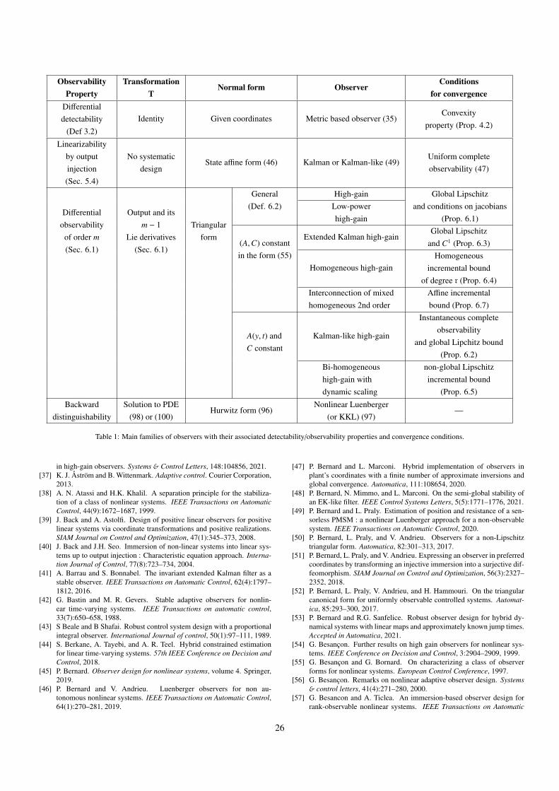
ObservabilityProperty
TransformationT
Normal form ObserverConditions
for convergenceDifferentialdetectability
(Def 3.2)Identity Given coordinates Metric based observer (35)
Convexityproperty (Prop. 4.2)
Linearizabilityby outputinjection(Sec. 5.4)
No systematicdesign
State affine form (46) Kalman or Kalman-like (49)Uniform completeobservability (47)
Differentialobservability
of order m(Sec. 6.1)
Output and itsm − 1
Lie derivatives(Sec. 6.1)
Triangularform
General(Def. 6.2)
High-gain Global Lipschitzand conditions on jacobians
(Prop. 6.1)Low-powerhigh-gain
(A,C) constantin the form (55)
Extended Kalman high-gainGlobal Lipschitz
and C1 (Prop. 6.3)
Homogeneous high-gainHomogeneous
incremental boundof degree r (Prop. 6.4)
Interconnection of mixedhomogeneous 2nd order
Affine incrementalbound (Prop. 6.7)
A(y, t) andC constant
Kalman-like high-gain
Instantaneous completeobservability
and global Lipchitz bound(Prop. 6.2)
Bi-homogeneoushigh-gain withdynamic scaling
non-global Lipschitzincremental bound
(Prop. 6.5)
Backwarddistinguishability
Solution to PDE(98) or (100)
Hurwitz form (96)Nonlinear Luenberger
(or KKL) (97)—
Table 1: Main families of observers with their associated detectability/observability properties and convergence conditions.
in high-gain observers. Systems & Control Letters, 148:104856, 2021.[37] K. J. Åstrom and B. Wittenmark. Adaptive control. Courier Corporation,
2013.[38] A. N. Atassi and H.K. Khalil. A separation principle for the stabiliza-
tion of a class of nonlinear systems. IEEE Transactions on AutomaticControl, 44(9):1672–1687, 1999.
[39] J. Back and A. Astolfi. Design of positive linear observers for positivelinear systems via coordinate transformations and positive realizations.SIAM Journal on Control and Optimization, 47(1):345–373, 2008.
[40] J. Back and J.H. Seo. Immersion of non-linear systems into linear sys-tems up to output injection : Characteristic equation approach. Interna-tion Journal of Control, 77(8):723–734, 2004.
[41] A. Barrau and S. Bonnabel. The invariant extended Kalman filter as astable observer. IEEE Transactions on Automatic Control, 62(4):1797–1812, 2016.
[42] G. Bastin and M. R. Gevers. Stable adaptive observers for nonlin-ear time-varying systems. IEEE Transactions on automatic control,33(7):650–658, 1988.
[43] S Beale and B Shafai. Robust control system design with a proportionalintegral observer. International Journal of control, 50(1):97–111, 1989.
[44] S. Berkane, A. Tayebi, and A. R. Teel. Hybrid constrained estimationfor linear time-varying systems. 57th IEEE Conference on Decision andControl, 2018.
[45] P. Bernard. Observer design for nonlinear systems, volume 4. Springer,2019.
[46] P. Bernard and V. Andrieu. Luenberger observers for non au-tonomous nonlinear systems. IEEE Transactions on Automatic Control,64(1):270–281, 2019.
[47] P. Bernard and L. Marconi. Hybrid implementation of observers inplant’s coordinates with a finite number of approximate inversions andglobal convergence. Automatica, 111:108654, 2020.
[48] P. Bernard, N. Mimmo, and L. Marconi. On the semi-global stability ofan EK-like filter. IEEE Control Systems Letters, 5(5):1771–1776, 2021.
[49] P. Bernard and L. Praly. Estimation of position and resistance of a sen-sorless PMSM : a nonlinear Luenberger approach for a non-observablesystem. IEEE Transactions on Automatic Control, 2020.
[50] P. Bernard, L. Praly, and V. Andrieu. Observers for a non-Lipschitztriangular form. Automatica, 82:301–313, 2017.
[51] P. Bernard, L. Praly, and V. Andrieu. Expressing an observer in preferredcoordinates by transforming an injective immersion into a surjective dif-feomorphism. SIAM Journal on Control and Optimization, 56(3):2327–2352, 2018.
[52] P. Bernard, L. Praly, V. Andrieu, and H. Hammouri. On the triangularcanonical form for uniformly observable controlled systems. Automat-ica, 85:293–300, 2017.
[53] P. Bernard and R.G. Sanfelice. Robust observer design for hybrid dy-namical systems with linear maps and approximately known jump times.Accepted in Automatica, 2021.
[54] G. Besancon. Further results on high gain observers for nonlinear sys-tems. IEEE Conference on Decision and Control, 3:2904–2909, 1999.
[55] G. Besancon and G. Bornard. On characterizing a class of observerforms for nonlinear systems. European Control Conference, 1997.
[56] G. Besancon. Remarks on nonlinear adaptive observer design. Systems& control letters, 41(4):271–280, 2000.
[57] G. Besancon and A. Ticlea. An immersion-based observer design forrank-observable nonlinear systems. IEEE Transactions on Automatic
26
Control, 52(1):83–88, 2007.[58] G. Besancon and A. Ticlea. On adaptive observers for systems with state
and parameter nonlinearities. IFAC-PapersOnLine, 50(1):15416–15421,2017.
[59] P. Blondel, R. Postoyan, S. Rael, S. Benjamin, and P. Desprez. Non-linear circle-criterion observer design for an electrochemical batterymodel. IEEE Transactions on Control Systems Technology, 27(2):889–897, 2018.
[60] N. Boizot, E. Busvelle, and J-P. Gauthier. An adaptive high-gain ob-server for nonlinear systems. Automatica, 46(9):1483–1488, 2010.
[61] S. Bonnabel. Left-invariant extended Kalman filter and attitude estima-tion. In 2007 46th IEEE Conference on Decision and Control, pages1027–1032. IEEE, 2007.
[62] S. Bonnabel, A. Astolfi, and R. Sepulchre. Contraction and observer de-sign on cones. In 2011 50th IEEE Conference on Decision and Controland European Control Conference, pages 7147–7151. IEEE, 2011.
[63] S. Bonnabel and J-J. Slotine. A contraction theory-based analysis of thestability of the deterministic extended Kalman filter. IEEE Transactionson Automatic Control, 60(2):565–569, 2015.
[64] G. Bornard, F. Celle-Couenne, and G. Gilles. Nonlinear systems, Mod-eling and Estimation 1, chapter Observability and observers, pages 173–216. Springer US, 1995.
[65] G. Bornard, N. Couenne, and F. Celle. Regularly persistent observers forbilinear systems. In J. Descusse, M. Fliess, A. Isidori, and D. Leborgne,editors, New Trends in Nonlinear Control Theory, pages 130–140,Berlin, Heidelberg, 1989. Springer Berlin Heidelberg.
[66] D. Bossane, D. Rakotopara, and J-P. Gauthier. Local and global im-mersion into linear systems up to output injection. IEEE Conference onDecision and Control, pages 2000–2004, 1989.
[67] M. Boutayeb, H. Rafaralahy, and M. Darouach. Convergence analysis ofthe extended Kalman filter used as an observer for nonlinear determin-istic discrete-time systems. IEEE Transactions on Automatic Control,42(4):581–586, 1997.
[68] L. Brivadis, V. Andrieu, E. Chabanon, E. Gagniere, N. Lebaz, andU. Serres. New dynamical observer for a batch crystallization processbased on solute concentration. Journal of Process Control, 87:17–26,2020.
[69] E. Bullinger and F. Allgower. An adaptive high-gain observer for non-linear systems. In Proceedings of the 36th IEEE Conference on Decisionand Control, volume 5, pages 4348–4353. IEEE, 1997.
[70] K. K. Busawon and P. Kabore. Disturbance attenuation using propor-tional integral observers. International Journal of control, 74(6):618–627, 2001.
[71] R. Carroll and D. Lindorff. An adaptive observer for single-inputsingle-output linear systems. IEEE Transactions on Automatic Control,18(5):428–435, 1973.
[72] A. Chalanga, S. Kamal, L. M. Fridman, B. Bandyopadhyay, and J. A.Moreno. Implementation of super-twisting control: Super-twisting andhigher order sliding-mode observer-based approaches. IEEE Transac-tions on Industrial Electronics, 63(6):3677–3685, 2016.
[73] C-T. Chen. Linear system theory and design. CBS College Publishing,1984.
[74] Y. Chitour. Time-varying high-gain observers for numerical differentia-tion. IEEE Transactions on Automatic Control, 47(9):1565–1569, 2002.
[75] Y. M. Cho and R. Rajamani. A systematic approach to adaptive ob-server synthesis for nonlinear systems. IEEE transactions on AutomaticControl, 42(4):534–537, 1997.
[76] M. S. Chong, D. Nesic, R. Postoyan, and L. Kuhlmann. Parameterand state estimation of nonlinear systems using a multi-observer underthe supervisory framework. IEEE Transactions on Automatic Control,60(9):2336–2349, 2015.
[77] G. Ciccarella, M. Dalla Mora, and A. Germani. A Luenberger-likeobserver for nonlinear systems. International Journal of Control,57(3):537–556, 1993.
[78] G. Clement, B.and Duc. An interpolation method for gain-scheduling.In Proceedings of the 40th IEEE Conference on Decision and Control(Cat. No. 01CH37228), volume 2, pages 1310–1315. IEEE, 2001.
[79] M. Cocetti, S. Tarbouriech, and L. Zaccarian. On dead-zone observersfor linear plants. In 2018 Annual American Control Conference (ACC),pages 5138–5143. IEEE, 2018.
[80] E. Cruz-Zavala and J. A. Moreno. Levant’s arbitrary-order exact dif-
ferentiator: A Lyapunov approach. IEEE Transactions on AutomaticControl, 64(7):3034–3039, 2019.
[81] L. da Costa Ramos, F. Di Meglio, V. Morgenthaler, L. F. Figueirada Silva, and P. Bernard. Numerical design of Luenberger observersfor nonlinear systems. In IEEE Conference on Decision and Control,pages 5435–5442, 2020.
[82] F. Deza, E. Busvelle, J-P. Gauthier, and D. Rakotopara. High gain esti-mation for nonlinear systems. Systems & control letters, 18(4):295–299,1992.
[83] T. N. Dinh, V. Andrieu, M. Nadri, and U. Serres. Continuous-discretetime observer design for Lipschitz systems with sampled measurements.IEEE Transactions on Automatic Control, 60(3):787–792, 2015.
[84] D. Efimov, A. Polyakov, A. Levant, and W. Perruquetti. Convergenceacceleration for observers by gain commutation. International Journalof Control, 91(9):2009–2018, 2018.
[85] D. Efimov, T. Raıssi, S. Chebotarev, and A. Zolghadri. Interval stateobserver for nonlinear time varying systems. Automatica, 49(1):200–205, 2013.
[86] S.V. Emelyanov, S.K. Korovin, S.V. Nikitin, and M.G. Nikitina. Ob-servers and output differentiators for nonlinear systems. DokladyAkademii Nauk, 306:556–560, 1989.
[87] R. Engel. Nonlinear observers for Lipschitz continuous systems withinputs. International Journal of Control, 80(4):495–508, 2007.
[88] R. Engel and G. Kreisselmeier. A continuous-time observer whichconverges in finite time. IEEE Transactions on Automatic Control,47(7):1202–1204, 2002.
[89] F. Esfandiari and H.K. Khalil. Observer-based design of uncertain sys-tems: recovering state feedback robustness under matching conditions.In Proceedings of Allerton Conference, Monticello, IL, pages 97––106,1987.
[90] K. Esfandiari and M. Shakarami. Bank of high-gain observers in outputfeedback control: Robustness analysis against measurement noise. IEEETransactions on Systems, Man, and Cybernetics: Systems, 2019.
[91] L. Etienne, S. Di Gennaro, and J-P. Barbot. Periodic event-triggeredobservation and control for nonlinear Lipschitz systems using impul-sive observers. International Journal of Robust and Nonlinear Control,27(18):4363–4380, 2017.
[92] L. Etienne, L. Hetel, D. Efimov, and M. Petreczky. Observer synthesisunder time-varying sampling for Lipschitz nonlinear systems. Automat-ica, 85:433 – 440, 2017.
[93] X. Fan and M. Arcak. Observer design for systems with multivariablemonotone nonlinearities. Systems & Control Letters, 50(4):319–330,2003.
[94] L. Farina and S. Rinaldi. Positive linear systems: theory and applica-tions, volume 50. John Wiley & Sons, 2011.
[95] M. Farza, M. M’Saad, M. L. Fall, E. Pigeon, O. Gehan, and K. Busawon.Continuous-discrete time observers for a class of MIMO nonlinear sys-tems. IEEE Transactions on Automatic Control, 59(4):1060–1065, 2014.
[96] M. Farza, M. M’Saad, T. Maatoug, and M. Kamoun. Adaptive observersfor nonlinearly parameterized class of nonlinear systems. Automatica,45(10):2292–2299, 2009.
[97] M. Farza, M. Oueder, R. B. Abdennour, and M. M’Saad. High gainobserver with updated gain for a class of MIMO nonlinear systems. In-ternational Journal of Control, 84(2):270–280, 2011.
[98] F. Ferrante, F. Gouaisbaut, R. G. Sanfelice, and S. Tarbouriech. Stateestimation of linear systems in the presence of sporadic measurements.Automatica, 73:101–109, 2016.
[99] M. Fliess. Generalized controller canonical form for linear and nonlineardynamics. IEEE Transactions on Automatic Control, 35(9):994–1001,1990.
[100] M. Fliess and I. Kupka. A finiteness criterion for nonlinear input-output differential systems. SIAM Journal of Control and Optimization,21(5):721–728, 1983.
[101] T. Floquet and J.P. Barbot. Super twisting algorithm-based step-by-stepsliding mode observers for nonlinear systems with unknown inputs. In-ternational journal of systems science, 38(10):803–815, 2007.
[102] F. J. Franquiz, J. D. Mu noz, B. Udrea, and M. J. Balas. Optimalrange observability maneuvers of a spacecraft formation using angles-only navigation. Acta Astronautica, 153:337 – 348, 2018.
[103] J. Gauthier and G. Bornard. Observability for any u(t) of a class of non-linear systems. IEEE Transactions on Automatic Control, 26(4):922–
27
926, 1981.[104] J-P. Gauthier, H. Hammouri, and S. Othman. A simple observer for
nonlinear systems applications to bioreactors. IEEE Transactions onAutomatic Control, 37(6):875–880, 1992.
[105] J.-P. Gauthier and I. Kupka. Deterministic observation theory and ap-plications. Cambridge university press, 2001.
[106] R. Goebel, R. G. Sanfelice, and A. R. Teel. Hybrid dynamical systems:modeling stability, and robustness, 2012.
[107] J.L. Gouze, A. Rapaport, and M.Z. Hady-Sadok. Interval observers foruncertain biological systems. Ecological Modelling, 133:45–56, 2000.
[108] M. Guay. Observer linearization by output-dependent time-scale trans-formations. IEEE Transactions on Automatic Control, 47(10):1730 –1735, 2002.
[109] B.-Z. Guo and Z.-L. Zhao. On the convergence of an extended stateobserver for nonlinear systems with uncertainty. Systems & Control Let-ters, 60(6):420–430, 2011.
[110] T. Hamel and R. Mahony. Attitude estimation on SO(3) based on directinertial measurements. In Proceedings 2006 IEEE International Confer-ence on Robotics and Automation, 2006. ICRA 2006., pages 2170–2175.IEEE, 2006.
[111] H. Hammouri, F.S. Ahmed, and S. Othman. Observer design basedon immersion technics and canonical form. Systems & Control Letters,114:19–26, 2018.
[112] H. Hammouri and M. Kinnaert. A new procedure for time-varying lin-earization up to output injection. Systems & Control Letters, 28:151–157, 1996.
[113] H. Hammouri and J. De Leon Morales. Observer synthesis for state-affine systems. IEEE Conference on Decision and Control, pages 784–785, 1990.
[114] H. Hammouri, H. G. Vu, and H. Yahoui. Local observer for infinitesi-mally observable nonlinear systems. International Journal of Control,86(4):579–590, 2013.
[115] W.P.M.H. Heemels, M.K. Camlibel, and M.F. Heertjes. Oblique pro-jected dynamical systems and incremental stability under state con-straints. IEEE Control Systems Letters, 4(4):1060–1065, 2020.
[116] B. T. Hinson, M. K. Binder, and K. A. Morgansen. Path planning tooptimize observability in a planar uniform flow field. In 2013 AmericanControl Conference, pages 1392–1399, 2013.
[117] B. T. Hinson and K. A. Morgansen. Observability optimization for thenonholonomic integrator. In 2013 American Control Conference, pages4257–4262, 2013.
[118] G-D. Hu. Observers for one-sided Lipschitz non-linear systems. IMAJournal of Mathematical Control and Information, 23(4):395–401,2006.
[119] S. Ibrir. LPV approach to continuous and discrete nonlinear observerdesign. In Proceedings of the 48h IEEE Conference on Decision andControl (CDC) held jointly with 2009 28th Chinese Control Conference,pages 8206–8211. IEEE, 2009.
[120] S. Ibrir and S. Diop. On continuous time differentiation observers. In1999 European Control Conference (ECC), pages 2402–2406. IEEE,1999.
[121] P. A. Ioannou and J. Sun. Robust Adaptive Control. Prentice Hall, Inc,1995.
[122] A. Isidori. Lectures in Feedback Design for Multivariable Systems.Springer, 2017.
[123] A. H. Jazwinski. Stochastic processes and filtering theory. AcademicPress, 1970.
[124] A. Jbara, A. Levant, and A. Hanan. Filtering homogeneous observers incontrol of integrator chains. International Journal of Robust and Non-linear Control, 31(9):3658–3685, 2021.
[125] L.S. Jennings, T.L. Fernando, and H. M. Trinh. Existence conditions forfunctional observability from an eigenspace perspective. IEEE Transac-tions on Automatic Control, 56(12):2957–2961, 2011.
[126] P. Jouan. Immersion of nonlinear systems into linear systems mod-ulo output injection. SIAM Journal on Control and Optimization,41(6):1756–1778, 2003.
[127] R. E. Kalman and R. S. Bucy. New results in linear filtering and predic-tion theory. Journal of Basic Engineering, 108:83–95, 1961.
[128] W. Kang, A. J. Krener, M. Xiao, and L. Xu. A survey of observers fornonlinear dynamical systems. In Data Assimilation for Atmospheric,Oceanic and Hydrologic Applications (Vol. II), pages 1–25. Springer,
2013.[129] D. Karagiannis and A. Astolfi. Nonlinear observer design using invariant
manifolds and applications. IEEE Conference on Decision and Controland European Control Conference, 2005.
[130] N. Kazantzis and C. Kravaris. Nonlinear observer design using Lya-punov’s auxiliary theorem. Systems and Control Letters, 34:241–247,1998.
[131] H. Keller. Nonlinear observer by transformation into a generalizedobserver canonical form. Internation Journal of Control, 46(6):1915–1930, 1987.
[132] H. K. Khalil and L. Praly. High-gain observers in nonlinear feedbackcontrol. Int. J. Robust. Nonlinear Control, 24, April 2013.
[133] H.K. Khalil. Cascade high-gain observers in output feedback control.Automatica, 80:110–118, 2017.
[134] A. Khan, W. Xie, Z. Bo, and L.-W. Liu. A survey of interval observersdesign methods and implementation for uncertain systems. Journal ofthe Franklin Institute, 2021.
[135] S. R. Kou, D. L. Elliott, and T. J. Tarn. Exponential observers for non-linear dynamic systems. Information and control, 29(3):204–216, 1975.
[136] C. Kravaris. Functional observers for nonlinear systems. IFAC Sympo-sium on Nonlinear Control Systems NOLCOS, 49(18):505–510, 2016.
[137] G. Kreisselmeier and R. Engel. Nonlinear observers for autonomouslipshitz continuous systems. IEEE Transactions on Automatic Control,48(3):451–464, 2003.
[138] A. J. Krener and W. Respondek. Nonlinear observers with linearizabledynamics. SIAM Journal of Control and Optimization, 23(2):197–216,1985.
[139] A.J. Krener. The convergence of the extended Kalman filter. In Direc-tions in mathematical systems theory and optimization, pages 173–182.Springer, 2003.
[140] A.J. Krener and A. Duarte. A hybrid computational approach to non-linear estimation. In Proceedings of 35th IEEE Conference on Decisionand Control, volume 2, pages 1815–1819. IEEE, 1996.
[141] A.J. Krener and A. Isidori. Linearization by output injection and non-linear observers. Systems & Control Letters, 3:47–52, 1983.
[142] A.J. Krener and M. Xiao. Nonlinear observer design in the Siegel do-main. SIAM Journal on Control and Optimization, 41(3):932–953, 2003.
[143] R. Krishnamurthy, F. Khorrami, and R.S. Chandra. Global high-gain-based observer and backstepping controller for generalized output-feedback canonical form. IEEE Transactions on Automatic Control,48(12):2277–2283, 2003.
[144] M. Krstic, P. V. Kokotovic, and I. Kanellakopoulos. Nonlinear and adap-tive control design. John Wiley & Sons, Inc., 1995.
[145] C. Lageman, J. Trumpf, and R. Mahony. Gradient-like observers forinvariant dynamics on a Lie group. IEEE Transactions on AutomaticControl, 55(2):367–377, 2009.
[146] H. Lei, J. Wei, and W. Lin. A global observer for observable autonomoussystems with bounded solution trajectories. In Proceedings of the 44thIEEE Conference on Decision and Control, pages 1911–1916. IEEE,2005.
[147] A. Levant. Higher-order sliding modes and arbitrary-order exact robustdifferentiation. Proceedings of the European Control Conference, pages996–1001, 2001 b.
[148] A. Levant. Higher-order sliding modes, differentiation and output-feedback control. International Journal of Control, 76(9-10):924–941,2003.
[149] A. Levant. Homogeneity approach to high-order sliding mode design.Automatica, 41(5):823–830, 2005.
[150] Y. Li, S. Phillips, and R.G. Sanfelice. Robust distributed estimation forlinear systems under intermittent information. IEEE Transactions onAutomatic Control, 63(4):973–988, 2017.
[151] Y. Li and R. G. Sanfelice. A finite-time convergent observer with robust-ness to piecewise-constant measurement noise. Automatica, 57:222–230, 2015.
[152] H. Lin, G. Zhai, and P. J. Antsaklis. Set-valued observer design for aclass of uncertain linear systems with persistent disturbance. AmericanControl Conference, 2003.
[153] Winfried Lohmiller and Jean-Jacques E Slotine. On contraction analysisfor non-linear systems. Automatica, 34(6):683–696, 1998.
[154] F. Lopez-Ramirez, A. Polyakov, D. Efimov, and W. Perruquetti. Finite-time and fixed-time observer design: Implicit lyapunov function ap-
28
proach. Automatica, 87:52–60, 2018.[155] L.Praly. On observers with state independent error lyapunov function.
IFAC Proceedings Volumes, 34(6):1349–1354, 2001.[156] G. Luders and K.S. Narendra. An adaptive observer and identifier for a
linear system. IEEE Transactions on Automatic Control, 18(5):496–499,1973.
[157] D. Luenberger. Observing the state of a linear system. IEEE Transac-tions on Military Electronics, 8:74–80, 1964.
[158] M. Maggiore and K. M. Passino. A separation principle for aclass of non-uco systems. IEEE Transactions on Automatic Control,48(7):1122–1133, 2003.
[159] R. Mahony, T. Hamel, and J.-M. Pflimlin. Nonlinear complementaryfilters on the special orthogonal group. IEEE Transactions on automaticcontrol, 53(5):1203–1218, 2008.
[160] R. Mahony, T. Hamel, and J. Trumpf. Equivariant systems theory andobserver design. arXiv preprint arXiv:2006.08276, 2020.
[161] J. Malaize, L. Praly, and N. Henwood. Globally convergent nonlinearobserver for the sensorless control of surface-mount permanent mag-net synchronous machines. IEEE Conference on Decision and Control,2012.
[162] I.R. Manchester. Contracting nonlinear observers: Convex optimizationand learning from data. In 2018 Annual American Control Conference(ACC), pages 1873–1880. IEEE, 2018.
[163] L. Marconi and L. Praly. Uniform practical nonlinear output regulation.IEEE Transactions on Automatic Control, 53:1184–1202, 2008.
[164] R. Marino. Adaptive observers for single output nonlinear systems.IEEE Transactions on Automatic Control, 35(9):1054–1058, 1990.
[165] Philippe Martin and Erwan Salaun. Generalized multiplicative extendedKalman filter for aided attitude and heading reference system. In AIAAGuidance, Navigation, and Control Conference, page 8300, 2010.
[166] F. Mazenc, V. Andrieu, and M. Malisoff. Design of continuous-discreteobservers for time-varying nonlinear systems. Automatica, 57:135 –144, 2015.
[167] F. Mazenc and O. Bernard. Interval observers for linear time-invariantsystems with disturbances. Automatica, 47(1):140–147, 2011.
[168] E. J. McShane. Extension of range of functions. Bull. Amer. Math. Soc.,40(12):837–842, 1934.
[169] L. Menini, C. Possieri, and A. Tornambe. A ”practical” observer fornonlinear systems. IEEE Conference on Decision and Control, pages3015–3020, 2017.
[170] L. Menini, C. Possieri, and A. Tornambe. Observers for linear systemsby the time integrals and moving average of the output. IEEE Transac-tions on Automatic Control, 64(12):4859–4874, 2019.
[171] L. Menini, C. Possieri, and A. Tornambe. On the use of the time-integrals of the output in observer design for non-linear autonomoussystem. IEEE Transactions on Automatic Control, 2021.
[172] P.H. Menold, R. Findeisen, and F. Allgower. Finite time convergentobservers for nonlinear systems. In 42nd IEEE International Conferenceon Decision and Control (IEEE Cat. No. 03CH37475), volume 6, pages5673–5678. IEEE, 2003.
[173] M. Dalla Mora, A. Germani, and C. Manes. Design of state observersfrom a drift-observability property. IEEE Transactions on AutomaticControl, 45(8):1536–1540, 2000.
[174] J. Moreno. Levant’s differentiator by interconnection of low orderblocks. In Third IFAC Conference on Modelling, Identification and Con-trol of Nonlinear Systems, 2021.
[175] S. Nazrulla and H.K. Khalil. Robust stabilization of non-minimum phasenonlinear systems using extended high-gain observers. IEEE Transac-tions on Automatic Control, 56(4):802–813, 2010.
[176] H. H. Niemann, J. Stoustrup, B. Shafai, and S. Beale. LTR design ofproportional-integral observers. International Journal of Robust andNonlinear Control, 5(7):671–693, 1995.
[177] R. Ortega, S. Aranovskiy, A. A. Pyrkin, A. Astolfi, and A. A. Bobtsov.New results on parameter estimation via dynamic regressor extensionand mixing: Continuous and discrete-time cases. IEEE Transactions onAutomatic Control, 66(5):2265–2272, 2020.
[178] W. Perruquetti, T. Floquet, and E. Moulay. Finite-time observers: ap-plication to secure communication. IEEE Transactions on AutomaticControl, 53(1):356–360, 2008.
[179] E. Petri, R. Postoyan, D. Astolfi, D. Nesic, and W.P.M.H. Heemels.Event-triggered observer design for linear systems. In 60th IEEE Con-
ference on Decision and Control, 2021.[180] K.S. Phogat and D.E. Chang. Invariant extended Kalman filter on matrix
Lie groups. Automatica, 114:108812, 2020.[181] F. Plestan and A. Glumineau. Linearization by generalized input-output
injection. Systems & Control Letters, 31:115–128, 1997.[182] R. Postoyan, M.H.A. Hamid, and J. Daafouz. A multi-observer approach
for the state estimation of nonlinear systems. In 2015 54th IEEE Con-ference on Decision and Control (CDC), pages 1793–1798. IEEE, 2015.
[183] R. Postoyan and D. Nesic. A framework for the observer design fornetworked control systems. IEEE Transactions on Automatic Control,57(5):1309–1314, 2011.
[184] R. Postoyan and D. Nesic. On emulated nonlinear reduced-order ob-servers for networked control systems. Automatica, 48(4):645–652,2012.
[185] L. Praly. Asymptotic stabilization via output feedback for lower triangu-lar systems with output dependent incremental rate. IEEE Transactionson Automatic Control, 48(6):1103–1108, 2003.
[186] L. Praly. Observers for nonlinear systems. In Baillieul J., Samad T. (eds)Encyclopedia of Systems and Control. Springer, 2015.
[187] L. Praly and Z.-P. Jiang. Stabilization by output feedback for systemswith ISS inverse dynamics. Systems & Control Letters, 21(1):19–33,1993.
[188] T.P. Proychev and R.L. Mishkov. Transformation of nonlinear systemsin observer canonical form with reduced dependency on derivatives ofthe input. Automatica, 29(2):495–498, 1993.
[189] C. Qian. A homogeneous domination approach for global output feed-back stabilization of a class of nonlinear systems. Proceedings of theAmerican Control Conference, 2005.
[190] C. Qian. A homogeneous domination approach for global output feed-back stabilization of a class of nonlinear systems. IEEE American Con-trol Conference, pages 4708–4715, 2005.
[191] C. Qian and W. Lin. Recursive observer design, homogeneous approx-imation, and nonsmooth output feedback stabilization of nonlinear sys-tems. IEEE Transactions on Automatic Control, 51(9), 2006.
[192] D. Rabehi, N. Meslem, and N. Ramdani. Finite-gain L1 event-triggeredinterval observers design for continuous-time linear systems. Inter-national Journal of Robust and Nonlinear Control, 31(9):4131–4153,2021.
[193] A. Radke and Z. Gao. A survey of state and disturbance observers forpractitioners. In American Control Conference, pages 6–11, 2006.
[194] T. Raff and F. Allgower. Observers with impulsive dynamical behaviorfor linear and nonlinear continuous-time systems. IEEE Conference onDecision and Control, pages 4287–4292, 2007.
[195] T. Raff, M. Kogel, and F. Allgower. Observer with sample-and-hold up-dating for Lipschitz nonlinear systems with nonuniformly sampled mea-surements. In 2008 American Control Conference, pages 5254–5257,2008.
[196] S. Raghavan and J. K. Hedrick. Observer design for a class of nonlinearsystems. International Journal of Control, 59(2):515–528, 1994.
[197] R. Rajamani. Observers for Lipschitz nonlinear systems. IEEE transac-tions on Automatic Control, 43(3):397–401, 1998.
[198] K. Rapp and P.-O. Nyman. Stability properties of the discrete-time ex-tended Kalman filter. IFAC Symposium on Nonlinear Control Systems,37(13):1377 – 1382, 2004.
[199] K. Reif, F. Sonnemann, and R. Unbehauen. An EKF-based nonlinearobserver with a prescribed degree of stability. Automatica, 34(9):1119–1123, 1998.
[200] W. Respondek, A. Pogromski, and H. Nijmeijer. Time scaling for ob-server design with linearizable error dynamics. Automatica, 40:277–285, 2004.
[201] H. Rıos and A. R. Teel. A hybrid observer for fixed-time state estima-tion of linear systems. In 2016 IEEE 55th Conference on Decision andControl (CDC), pages 5408–5413. IEEE, 2016.
[202] F. Rotella and I. Zambettakis. On functional observers for linear time-varying systems. IEEE Transactions on Automatic Control, 58(5):1354–1360, 2013.
[203] I. Rubio Scola, G. Besancon, and D. Georges. Optimizing Kalman op-timal observer for state affine systems by input selection. Automatica,93:224 – 230, 2018.
[204] J. Rudolph and M. Zeitz. A block triangular nonlinear observer normalform. Systems & Control Letters, 23(1):1–8, 1994.
29
[205] L. Sacchelli, L. Brivadis, V. Andrieu, U. Serres, and J.-P. Gauthier. Dy-namic output feedback stabilization of non-uniformly observable dissi-pative systems. IFAC-PapersOnLine, 53(2):4923–4928, 2020.
[206] P. Salaris, M. Cognetti, R. Spica, and P. R. Giordano. Online optimalperception-aware trajectory generation. IEEE Transactions on Robotics,35(6):1307–1322, 2019.
[207] S Salcudean. A globally convergent angular velocity observer for rigidbody motion. IEEE transactions on Automatic Control, 36(12):1493–1497, 1991.
[208] R. G. Sanfelice and L. Praly. Convergence of nonlinear observers onRn with a Riemannian metric (Part I). IEEE Transactions on AutomaticControl, 57(7):1709–1722, 2011.
[209] R. G. Sanfelice and L. Praly. On the performance of high-gain observerswith gain adaptation under measurement noise. Automatica, 47:2165–2176, 2011.
[210] R. G. Sanfelice and L. Praly. Convergence of nonlinear observers on Rn
with a Riemannian metric (Part II). IEEE Transactions on AutomaticControl, 61(10):2848–2860, 2015.
[211] M. M. Seron, J. H. Braslavsky, and G. C. Goodwin. Fundamental lim-itations in filtering and control. Springer Science & Business Media,2012.
[212] A. Sferlazza, S. Tarbouriech, and L. Zaccarian. Time-varying sampled-data observer with asynchronous measurements. IEEE Transactions onAutomatic Control, 64(2):869–876, 2019.
[213] D. Shi, T. Chen, and M. Darouach. Event-based state estimation of lineardynamic systems with unknown exogenous inputs. Automatica, 69:275–288, 2016.
[214] D. Shi, T. Chen, and L. Shi. Event-triggered maximum likelihood stateestimation. Automatica, 50(1):247–254, 2014.
[215] H. Shim and J.H. Jin Heon. Non-linear output feedback stabilizationon a bounded region of attraction. International Journal of Control,73(5):416–426, 2000.
[216] H. Shim and D. Liberzon. Nonlinear observers robust to measurementdisturbances in an ISS sense. IEEE Transactions on Automatic Control,61(1):48–61, 2016.
[217] H. Shim and L. Praly. Remarks on equivalence between full order andreduced order nonlinear observers. In 42nd IEEE International Con-ference on Decision and Control, volume 6, pages 5837–5840. IEEE,2003.
[218] A. Shoshitaishvili. On control branching systems with degenerate lin-earization. IFAC Symposium on Nonlinear Control Systems, pages 495–500, 1992.
[219] D. Simon. Kalman filtering with state constraints: a survey of linear andnonlinear algorithms. IET Control Theory & Applications, 4(8):1303–1318, 2010.
[220] Y. Song and J. W. Grizzle. The extended Kalman filter as a local asymp-totic observer for nonlinear discrete-time systems. American ControlConference, 29:3365 – 3369, 1992.
[221] E. D. Sontag. Input to state stability: Basic concepts and results. InNonlinear and optimal control theory, pages 163–220. Springer, 2008.
[222] E. D. Sontag and Y. Wang. Output-to-state stability and detectability ofnonlinear systems. Systems & Control Letters, 29(5):279–290, 1997.
[223] J. Sur and B. Paden. Observers for linear systems with quantized output.Annual American Control Conference, pages 3012–3016, 1997.
[224] A. Tanwani, B. Brogliato, and C. Prieur. Stability and observer designfor Lur’e systems with multivalued, nonmonotone, time-varying nonlin-earities and state jumps. SIAM Journal on Control and Optimization,52(6):3639–3672, 2014.
[225] A. Teel and L. Praly. Global stabilizability and observability imply semi-global stabilizability by output feedback. Systems & Control Letters,22(5):313–325, 1994.
[226] A.R. Teel. Further variants of the Astolfi/Marconi high-gain observer. In2016 american control conference (acc), pages 993–998. IEEE, 2016.
[227] F.E. Thau. Observing the state of non-linear dynamic systems. Interna-tional journal of control, 17(3):471–479, 1973.
[228] A. Tornambe. Use of asymptotic observers having high gains in the stateand parameter estimation. IEEE Conference on Decision and Control,2:1791–1794, 1989.
[229] C. Treangle, M. Farza, and M. M’Saad. Filtered high gain observer for aclass of uncertain nonlinear systems with sampled outputs. Automatica,101:197–206, 2019.
[230] J. Trumpf. Observers for linear time-varying systems. Linear Algebraand its Applications, 425:303–312, 2007.
[231] J. Tsinias. Observer design for nonlinear systems. Systems & ControlLetters, 13(2):135–142, 1989.
[232] I. Y. Tyukin, E. Steur, H. Nijmeijer, and C. Van Leeuwen. Adaptiveobservers and parameter estimation for a class of systems nonlinear inthe parameters. Automatica, 49(8):2409–2423, 2013.
[233] F.W.J. van den Berg, H.C.J. Hoefsloot, H.F.M. Boelens, and A.K.Smilde. Selection of optimal sensor position in a tubular reactor usingrobust degree of observability criteria. Chemical Engineering Science,55(4):827 – 837, 2000.
[234] K. Vijayaraghavan. Generalised observer design for dissipative Lips-chitz nonlinear systems in the presence of measurement noise. Interna-tional Journal of Control, 87(11):2273–2285, 2014.
[235] L. Wang, D. Astolfi, L. Marconi, and H. Su. High-gain observers withlimited gain power for systems with observability canonical form. Auto-matica, 75:16–23, 2017.
[236] B. Yang and W. Lin. Homogeneous observers, iterative design, andglobal stabilization of high-order nonlinear systems by smooth outputfeedback. IEEE Transactions on Automatic Control, 49(7):1069–1080,2004.
[237] M. Zeitz. Observability canonical (phase-variable) form for nonlin-ear time-variable systems. International Journal of Systems Science,15(9):949–958, 1984.
[238] M. Zeitz. The extended Luenberger observer for nonlinear systems. Sys-tems & Control Letters, 9(2):149–156, 1987.
[239] A. Zemouche, M. Boutayeb, and G.I. Bara. Observers for a class ofLipschitz systems with extension to h∞ performance analysis. Systems& Control Letters, 57(1):18–27, 2008.
[240] A. Zemouche, F. Zhang, F. Mazenc, and R. Rajamani. High-gain non-linear observer with lower tuning parameter. IEEE Transactions on Au-tomatic Control, 64(8):3194–3209, 2018.
[241] Q. Zhang. Adaptive observer for multiple-input-multiple-output(MIMO) linear time-varying systems. IEEE transactions on automaticcontrol, 47(3):525–529, 2002.
[242] G. Zimmer. State observation by on-line minimization. InternationalJournal of Control, 60(4):595–606, 1994.
30