robust adaptive dynamic programming for continuous -time ... · robust adaptive dynamic programming...
TRANSCRIPT
i
ROBUST ADAPTIVE DYNAMIC PROGRAMMING
FOR CONTINUOUS-TIME LINEAR AND
NONLINEAR SYSTEMS
DISSERTATION
Submitted in Partial Fulfillment of
The Requirements for
the Degree of
DOCTOR OF PHYLOSOPHY
(Electrical Engineering)
at the
NEW YORK UNIVERSITY
POLYTECHNIC SCHOOL OF ENGINEERING
by
Yu Jiang
May 2014
Approved:
__________________________ Department Head Signature
__________________________
Date
Copy No. #________
Students ID# N12872239
ii
Approved by the Guidance Committee
Major: Electrical Engineering
________________________________
Zhong-Ping Jiang
Professor of Electrical and Computer
Engineering
________________________________
Date
________________________________
Francisco de León
Associate Professor of Electrical and
Computer Engineering
________________________________
Date
________________________________
Peter Voltz
Associate Professor of Electrical and
Computer Engineering
________________________________
Date
Minor: Mathematics
________________________________
Gaoyong Zhang
Professor of Mathematics
________________________________
Date
iii
Microfilm or copies of this dissertation may be obtained from:
UMI Dissertation Publishing
ProQuest CSA
789 E. Eisenhower Parkway
P.O.Box 1346
Ann Arbor, MI 48106-1346
iv
Vita
Yu Jiang was born in Xi'an, China, in 1984. He obtained the B.Sc. degree in
Applied Mathematics from Sun Yat-sen University, Guangzhou, China, in
2006, and the M.Sc. degree in automation science and engineering
from South China University of Technology, Guangzhou, China, in 2009. He
won the National First Grade Award in the 2005 Chinese Undergraduate
Mathematical Contest in Modeling.
Currently, he is a fifth-year Ph.D. candidate working in the Control and
Networks (CAN) Lab at Polytechnic School of Engineering, New York
University, under the guidance of Professor Zhong-Ping Jiang. His research
interests include robust adaptive dynamic programming and its applications
in engineering and biological systems. In summer 2013, he interned
at Mitsubishi Electric Research Laboratories (MERL), Cambridge, MA. He
received the Shimemura Young Author Prize (with Zhong-Ping Jiang) at the
9th Asian Control Conference, Istanbul, Turkey, 2013.
v
List of publications
Book
1. Yu Jiang and Zhong-Ping Jiang, “Robust Adaptive Dynamic Programming”, in preparation.
Book Chapter
1. Yu Jiang and Zhong-Ping Jiang, "Robust adaptive dynamic programming", in Reinforcement
Learning and Approximate Dynamic Programming for Feedback Control, F. L. Lewis and D.
Liu, Eds, John Wiley and Sons, 2012.
Journal Papers (Under review)
1. Tao Bian, Yu Jiang and Zhong-Ping, “Adaptive dynamic programming for stochastic
systems with state and control dependent noise”, IEEE Transactions on Automatic Control,
submitted, April 2014.
2. Yu Jiang and Zhong-Ping Jiang, “Global adaptive dynamic programming for continuous-
time nonlinear systems,” IEEE Transactions on Automatic Control, submitted, Dec 2013.
3. Yu Jiang, Yebin Wang, Scott Bortoff, and Zhong-Ping Jiang, “Optimal Co-Design of
Nonlinear Control Systems Based on A Modified Policy Iteration Method,” IEEE
Transactions on Neural Networks and Learning Systems, major revision, Dec 2013.
4. Yu Jiang and Zhong-Ping Jiang, “A robust adaptive dynamic programming principle for
sensorimotor control with signal-dependent noise,” Journal of Systems Science and
Complexity, revised, Mar 2014.
5. Tao Bian, Yu Jiang, and Zhong-Ping Jiang, “Decentralized and adaptive optimal control of
large-scale systems with application to power systems”, IEEE Transactions on Industrial
Electronics, revised, Apr 2014.
6. Yu Jiang and Zhong-Ping Jiang, “Adaptive dynamic programming as a theory of
sensorimotor control,” Biological Cybernetics, revised Mar 2014.
Journal Papers (Published or accepted)
1. Yu Jiang, Yebin Wang, Scott Bortoff, and Zhong-Ping Jiang, “An Iterative Approach to the
Optimal Co-Design of Linear Control System,” Automatica, provisionally accepted.
2. Tao Bian, Yu Jiang, and Zhong-Ping Jiang, “Adaptive dynamic programming and optimal
control of nonlinear nonaffine systems,” Automatica, provisionally accepted.
vi
3. Yu Jiang and Zhong-Ping Jiang, “Robust adaptive dynamic programming and feedback
stabilization of Nonlinear Systems,” IEEE Transactions on Neural Networks and Learning
Systems, vol. 25, no. 5, pp. 882-893, May 2014.
4. Zhong-Ping Jiang and Yu Jiang, “Robust adaptive dynamic programming for linear and
nonlinear systems: An overview”, European Journal of Control, vol. 19, no. 5, pp. 417-425,
2013.
5. Yu Jiang and Zhong-Ping Jiang, "Robust adaptive dynamic programming with an application
to power systems", IEEE Transactions on Neural Networks and Learning Systems, vol. 24,
no.7, pp. 1150- 1156, 2013.
6. Yu Jiang and Zhong-Ping Jiang, "Robust adaptive dynamic programming for large-scale
systems with an application to multimachine power systems," IEEE Transactions on Circuits
and Systems, Part II, vol. 59, no. 10, pp. 693-697, 2012.
7. Ning Qian, Yu Jiang, Zhong-Ping Jiang, and Pietro Mazzoni, "Movement duration, Fitts's
law, and an infinite-horizon optimal feedback control model for biological motor systems",
Neural Computation, vol. 25, no. 3, pp. 697-724, 2012.
8. Yu Jiang and Zhong-Ping Jiang, "Computational adaptive optimal control for continuous-
time linear systems with completely unknown system dynamics", Automatica, vol. 48, no. 10,
pp. 2699-2704, Oct. 2012.
9. Yu Jiang and Zhong-Ping Jiang, "Approximate dynamic programming for optimal stationary
control with control-dependent noise," IEEE Transactions on Neural Networks, vol. 22, no.12,
2392-2398, 2011.
Conference Papers
1. Yu Jiang and Zhong-Ping Jiang, “Global adaptive dynamic programming and global optimal
control for a class of nonlinear systems”, accepted in the 2014 IFAC World Congress.
2. Yu Jiang, Zhong-Ping Jiang, “Robust adaptive dynamic programming for sensorimotor
control with signal-dependent noise,” in Proceedings of the 2013 IEEE Signal Processing in
Medicine and Biology Symposium, Brooklyn, NY, 2013.
3. Zhong-Ping Jiang and Yu Jiang, “Robust Adaptive Dynamic Programming: Recent results
and applications”, in Proceedings of the 32nd Chinese Control Conference, Xi'An, China, pp.
968-973, 2013.
4. Yu Jiang and Zhong-Ping Jiang, “Robust adaptive dynamic programming for optimal
nonlinear control,” in proceedings of the 9th Asian Control Conference. (Shimemura Young
Author Award).
vii
5. Zhong-Ping Jiang and Yu Jiang, “A new approach to robust and optimal nonlinear control
design,” the Third IASTED Asian Conference on Modeling, Identification and Control,
Phuket, Thailand, 2013.
6. Yu Jiang and Zhong-Ping Jiang, "Adaptive dynamic programming as a theory of motor
control", accepted in the 2012 IEEE Signal Processing in Medicine and Biology Symposium,
New York, NY, 2012.
7. Yu Jiang and Zhong-Ping Jiang, "Robust adaptive dynamic programming for nonlinear
control design," accepted in the51st IEEE Conference on Decision and Control, Dec. 2012,
Maui, Hawaii, USA.
8. Yu Jiang and Zhong-Ping Jiang, "Computational adaptive optimal control with an
application to blood glucose regulation in type 1 diabetics," in Proceedings of the 31th
Chinese Control Conference, Hefei, China, pp. 2938-2943, July, 2012.
9. Yu Jiang and Zhong-Ping Jiang, "Robust adaptive dynamic programming: An overview of
recent results", in Proceedings of the 20th International Symposium on Mathematical Theory
of Networks and Systems, Melbourne, Australia, 2012.
10. Yu Jiang and Zhong-Ping Jiang, "Robust approximate dynamic programming and global
stabilization with nonlinear dynamic uncertainties," in Proceedings of the Joint IEEE
Conference on Decision and Control and European Control Conference, Orlando, FL, USA,
pp. 115-120, 2011.
11. Yu Jiang, Srinivasa Chemudupati, Jan Morup Jorgensen, Zhong-Ping Jiang, and Charles S.
Peskin, "Optimal control mechanism involving the human kidney," in Proceedings of the
Joint IEEE Conference on Decision and Control and European Control Conference, Orlando,
FL, USA, pp. 3688-3693, 2011.
12. Yu Jiang and Zhong-Ping Jiang, "Approximate dynamic programming for stochastic systems
with additive and multiplicative noise," in Proceedings of the IEEE Multi-Conference on
Systems and Control, pp. 185-190, Denver, CO, 2011.
13. Yu Jiang, Zhong-Ping Jiang, and Ning Qian, "Optimal control mechanisms in human arm
reaching movements," in Proceedings of the 30th Chinese Control Conference, pp. 1377-
1382, Yantai, China, 2011.
14. Yu Jiang and Zhong-Ping Jiang, "Approximate dynamic programming for output feedback
control," in Proceedings of Chinese Control Conference, pp. 5815-5820, Beijing, China, 2010.
15. Yu Jiang and Jie Huang, "Output regulation for a class of weakly minimum phase systems
and its application to a nonlinear benchmark system," in Proceedings of American Control
Conference, pp. 5321-5326, St. Louis, USA, 2009.
viii
Acknowledgement
I would first and foremost like to thank Prof. Zhong-Ping Jiang. Without his
generous support and guidance, this dissertation would not have been
possible and it would remain incomplete if I did not thank him with utmost
sincerity. In the past five years, he not only introduced me to the exciting
topic of robust adaptive dynamic programming, but also set high goals for my
research and at the same time keeps helping and encouraging me to work
towards them. He gives me flexibility to work on any problem that interests
me, makes me question theories which I took for granted, and challenges me
to seek breakthroughs. Indeed, it was a great honor and pleasure working
under his guidance.
I would like to thank Prof. Charles Peskin at Courant Institute of
Mathematical Sciences (CIMS) and Prof. Ning Qian from Columbia
University for introducing me to the wonderful subjects of biological related
control problems.
I would like to thank Prof. Francisco de León for providing a lot of
constructive suggestions and professional advice when I was trying to apply
my theory to solve power systems related control problems.
I would also like to thank Dr. Yebin Wang at Mitsubishi Electric Research
Laboratories (MERL) for offering me a chance to intern at the prestigious
industrial research lab and to learn how to apply control theories to practical
engineering systems.
I would like to extend my heartfelt thanks to Prof. Peter Voltz, Prof. Gaoyong
Zhang, and Prof. Francisco de León for taking their valuable time reading
and reviewing my dissertation.
I would like to thank Srinivasa Chemudupati, Ritchy Laurent, Zhi Chen, Po-
Chen Chen, Xiyun Wang, Xinhe Chen, Qingcheng Zhu, Yang Xian, Xuesong
Lu, Siddhartha Srikantham, Tao Bian, Weinan Gao, Bei Sun, Jeffery Pawlick
and all my current and former fellow lab mates for creating a supportive,
productive, and fun environment.
Last but not least, I thank the National Science Foundation for supporting
my research work.

ix
To Misi – “a prudent wife is from the Lord”
x
Abstract
Robust Adaptive Dynamic Programming for Continuous-Time
Linear and Nonlinear Systems
By
Yu Jiang
Advisor: Zhong-Ping Jiang
Submitted in Partial Fulfillment of the Requirements for the Degree of
Doctor of Philosophy (Electrical Engineering)
May 2014
The field of adaptive dynamic programming and its applications to control
engineering problems has undergone rapid progress over the past few
years. Recently, a new theory called Robust Adaptive Dynamic Programming
(for short, RADP) has been developed for the design of robust optimal
controllers for linear and nonlinear systems subject to both parametric and
dynamic uncertainties. This dissertation integrates our recent contributions
to the development of the theory of RADP and illustrates its potential
applications in both engineering and biological systems.
In order to develop the RADP framework, our attention is first focused on the
development of an ADP-based online learning method for continuous-time
(CT) linear systems with completely unknown system. This problem is
challenging due to the different structures between CT and discrete-time (DT)
algebraic Riccati equations (AREs), and therefore methods developed for DT
ADP cannot be directly applied in the CT setting. This obstacle is overcome
in our work by taking advantages of exploration noise. The methodology is
xi
immediately extended to deal with CT affine nonlinear systems, via neural-
networks-based approximation of the Hamilton-Jacobi-Bellman (HJB)
equation, of which the solution is extremely difficult to be obtained
analytically. To achieve global stabilization, for the first time we propose an
idea of global ADP (or GADP), in which we relax the problem of solving the
Hamilton-Jacobi-Bellman (HJB) equation to an optimization problem, of
which a suboptimal solution is obtained via a sum-of-squares-program-based
policy iteration method. The resultant control policy is globally stabilizing,
instead of semi-globally or locally stabilizing.
Then, we develop RADP aimed at computing globally stabilizing and
suboptimal control policies in the presence of dynamic uncertainties. A key
strategy is to integrate ADP theory with techniques in modern nonlinear
control with a unique objective of filling a gap in the past literature of ADP
without taking into account dynamic uncertainties. The development of this
framework contains two major steps. First, we study an RADP method for
partially linear systems (i.e., linear systems with nonlinear dynamic
uncertainties) and weakly nonlinear large-scale systems. Global stabilization
of the systems can be achieved by selecting performance indices with
appropriate weights for the nominal system. Second, we extend the RADP
framework for affine nonlinear systems with nonlinear dynamic uncertainties.
To achieve robust stabilization, we resort to tools from nonlinear control
theory, such as gain assignment and the ISS nonlinear small-gain theorem.
From the perspective of RADP, we derive a novel computational mechanism
for sensorimotor control. Sharing some essential features of reinforcement
learning, which was originally observed from mammals, the RADP model for
sensorimotor control suggests that, instead of identifying the system
dynamics of both the motor system and the environment, the central nervous
system (CNS) computes iteratively a robust optimal control policy using the
real-time sensory data. By comparing our numerical results with
xii
experimentally observed data, we show that the proposed model can
reproduce movement trajectories which are consistent with experimental
observations. In addition, the RADP theory provides a unified framework
that connects optimality and robustness properties in the sensorimotor
system. Therefore, we argue that the CNS may use RADP-like learning
strategies to coordinate movements and to achieve successful adaptation in
the presence of static and/or dynamic uncertainties.
Contents
List of Figures xiv
List of Tables xvii
List of Symbols xviii
List of Abbreviations xix
1 Introduction 1
1.1 From RL to RADP . . . . . . . . . . . . . . . . . . . . . . . . . . . . 1
1.2 Contributions of this dissertation . . . . . . . . . . . . . . . . . . . . 7
2 ADP for linear systems with completely unknown dynamics 9
2.1 Problem formulation and preliminaries . . . . . . . . . . . . . . . . . 10
2.2 ADP-based online learning with completely unknown dynamics . . . 13
2.3 Application to a turbocharged diesel engine . . . . . . . . . . . . . . 20
2.4 Conclusions . . . . . . . . . . . . . . . . . . . . . . . . . . . . . . . . 24
3 RADP for uncertain partially linear systems 26
3.1 Problem formulation . . . . . . . . . . . . . . . . . . . . . . . . . . . 28
3.2 Optimality and robustness . . . . . . . . . . . . . . . . . . . . . . . . 28
3.3 RADP design . . . . . . . . . . . . . . . . . . . . . . . . . . . . . . . 32
3.4 Application to synchronous generators . . . . . . . . . . . . . . . . . 39
3.5 Conclusions . . . . . . . . . . . . . . . . . . . . . . . . . . . . . . . . 42
4 RADP for large-scale systems 43
4.1 Stability and optimality for large-scale systems . . . . . . . . . . . . . 44
4.2 The RADP design for large-scale systems . . . . . . . . . . . . . . . . 53
4.3 Application to a ten machine power system . . . . . . . . . . . . . . . 58
4.4 Conclusions . . . . . . . . . . . . . . . . . . . . . . . . . . . . . . . . 61
xiii
5 Neural-networks-based RADP for nonlinear systems 66
5.1 Problem formulation and preliminarlies . . . . . . . . . . . . . . . . . 67
5.2 Online Learning via RADP . . . . . . . . . . . . . . . . . . . . . . . 69
5.3 RADP with unmatched dynamic uncertainty . . . . . . . . . . . . . . 83
5.4 Numerical examples . . . . . . . . . . . . . . . . . . . . . . . . . . . . 90
5.5 Conclusions . . . . . . . . . . . . . . . . . . . . . . . . . . . . . . . . 98
6 Global robust adaptive dynamic programming via sum-of-squares-
programming 101
6.1 Problem formulation and preliminaries . . . . . . . . . . . . . . . . . 103
6.2 Suboptimal control with relaxed HJB equation . . . . . . . . . . . . . 109
6.3 SOS-based policy iteration for polynomial systems . . . . . . . . . . . 113
6.4 Online learning via global adaptive dynamic programming . . . . . . 120
6.5 Extension to nonpolynomial systems . . . . . . . . . . . . . . . . . . 124
6.6 Robust redesign . . . . . . . . . . . . . . . . . . . . . . . . . . . . . . 132
6.7 Numerical examples . . . . . . . . . . . . . . . . . . . . . . . . . . . . 137
6.8 Conclusions . . . . . . . . . . . . . . . . . . . . . . . . . . . . . . . . 144
7 RADP as a theory of sensorimotor control 147
7.1 ADP for continuous-time stochastic systems . . . . . . . . . . . . . . 150
7.2 RADP for continuous-time stochastic systems . . . . . . . . . . . . . 157
7.3 Numerical results: ADP-based sensorimotor control . . . . . . . . . . 176
7.4 Numerical results: RADP-based sensorimotor control . . . . . . . . . 192
7.5 Discussion . . . . . . . . . . . . . . . . . . . . . . . . . . . . . . . . . 199
7.6 Conclusions . . . . . . . . . . . . . . . . . . . . . . . . . . . . . . . . 205
8 Conclusions and future work 207
8.1 Conclusions . . . . . . . . . . . . . . . . . . . . . . . . . . . . . . . . 207
8.2 Future work . . . . . . . . . . . . . . . . . . . . . . . . . . . . . . . . 209
9 Appendices 211
9.1 Review of optimal control theory . . . . . . . . . . . . . . . . . . . . 211
9.2 Review of ISS and the nonlinear small-gain theorem . . . . . . . . . . 214
9.3 Matlab code for the simulation in Chapter 2 . . . . . . . . . . . . . . 217
Bibliography 222
xiv
List of Figures
1.1 Illustration of RL. . . . . . . . . . . . . . . . . . . . . . . . . . . . . . 2
1.2 Configuration of an ADP-based control system . . . . . . . . . . . . . 5
1.3 RADP with dynamic uncertainty. . . . . . . . . . . . . . . . . . . . . 6
2.1 Flowchart of Algorithm 2.2.1. . . . . . . . . . . . . . . . . . . . . . . 16
2.2 Trajectory of the Euclidean norm of the state variables during the
simulation. . . . . . . . . . . . . . . . . . . . . . . . . . . . . . . . . . 21
2.3 Trajectories of the output variables from t = 0s to t = 10s. . . . . . . 22
2.4 Convergence of Pk and Kk to their optimal values P ∗ and K∗ during
the learning process. . . . . . . . . . . . . . . . . . . . . . . . . . . . 23
3.1 Trajectories of the rotor angle. . . . . . . . . . . . . . . . . . . . . . . . 41
3.2 Trajectories of the angular velocity. . . . . . . . . . . . . . . . . . . . . 41
4.1 Power angle deviations of Generators 2-4. . . . . . . . . . . . . . . . . 62
4.2 Power angle deviations of Generators 5-7. . . . . . . . . . . . . . . . . 63
4.3 Power angle deviations of Generators 8-10. . . . . . . . . . . . . . . . 63
4.4 Power frequencies of Generators 2-4. . . . . . . . . . . . . . . . . . . 64
4.5 Power frequencies of Generators 5-7. . . . . . . . . . . . . . . . . . . 64
4.6 Power frequencies of Generators 8-10. . . . . . . . . . . . . . . . . . 65
5.1 Illustration of the nonlinear RADP algorithm . . . . . . . . . . . . . 82
5.2 Approximated cost function. . . . . . . . . . . . . . . . . . . . . . . . 93
5.3 Trajectory of the normalized rotating stall amplitude. . . . . . . . . . 94
5.4 Trajectory of the mass flow. . . . . . . . . . . . . . . . . . . . . . . . 95
5.5 Trajectory of the plenum pressure rise. . . . . . . . . . . . . . . . . . 96
5.6 One-machine infinite-bus synchronous generator with speed governor 97
5.7 Trajectory of the dynamic uncertainty. . . . . . . . . . . . . . . . . . 97
5.8 Trajectory of the deviation of the rotor angle. . . . . . . . . . . . . . 98
5.9 Trajectory of the relative frequency. . . . . . . . . . . . . . . . . . . . 99
xv
5.10 Trajectory of the deviation of the mechanical power. . . . . . . . . . . 99
5.11 Approximated cost function. . . . . . . . . . . . . . . . . . . . . . . . 100
6.1 Simulation of the scalar system: State trajectory . . . . . . . . . . . . 139
6.2 Simulation of the scalar system: Control input . . . . . . . . . . . . . 140
6.3 Simulation of the scalar system: Cost functions . . . . . . . . . . . . 140
6.4 Simulation of the scalar system: Control policies . . . . . . . . . . . . 141
6.5 Simulation of the inverted pendulum: State trajectories . . . . . . . . 143
6.6 Simulation of the inverted pendulum: Cost functions . . . . . . . . . 143
6.7 Simulation of the jet engine: Trajectories of r. . . . . . . . . . . . . . 145
6.8 Simulation of the jet engine: Trajectories of φ. . . . . . . . . . . . . . 145
6.9 Simulation of the jet engine: Value functions. . . . . . . . . . . . . . 146
7.1 RADP framework for sensorimotor control. . . . . . . . . . . . . . . . 159
7.2 Illustration of three weighting factors . . . . . . . . . . . . . . . . . . 179
7.3 Movement trajectories using the ADP-based learning scheme . . . . . 181
7.4 Simulated velocity and endpoint force curves . . . . . . . . . . . . . . 182
7.5 Illustration of the stiffness geometry to the VF . . . . . . . . . . . . . 183
7.6 Movement duration of the learning trials in the VF. . . . . . . . . . . 185
7.7 Illustration of stiffness geometry to the DF. . . . . . . . . . . . . . . 188
7.8 Simulated movement trajectories. . . . . . . . . . . . . . . . . . . . . 190
7.9 Simulated velocity and endpoint force curves . . . . . . . . . . . . . . 191
7.10 Log and power forms of Fitts’s law. . . . . . . . . . . . . . . . . . . . 193
7.11 Simulations of hand trajectories in the divergent force field . . . . . . 194
7.12 Adaptation of stiffness geometry to the force field. . . . . . . . . . . . 196
7.13 Simulation of hand trajectories in the velocity-dependent force field. . 198
7.14 Hand velocities before and after adaptation to the force field. . . . . . 200
xvi

List of Tables
4.1 Parameters for the generators . . . . . . . . . . . . . . . . . . . . . . 60
4.2 Imaginary parts of the admittance matrix . . . . . . . . . . . . . . . 60
4.3 Real parts of the admittance matrix . . . . . . . . . . . . . . . . . . . 61
7.1 Parameters of the linear model . . . . . . . . . . . . . . . . . . . . . 177
7.2 Data fitting for the log law and power law . . . . . . . . . . . . . . . 192
xvii
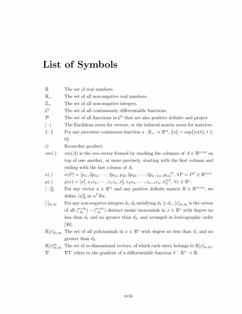
List of Symbols
R The set of real numbers.
R+ The set of all non-negative real numbers.
Z+ The set of all non-negative integers.
C1 The set of all continuously differentiable functions.
P The set of all functions in C1 that are also positive definite and proper.
| · | The Euclidean norm for vectors, or the induced matrix norm for matrices.
‖ · ‖ For any piecewise continuous function u : R+ → Rm, ‖u‖ = sup|u(t)|, t ≥0.
⊗ Kronecker product.
vec(·) vec(A) is the mn-vector formed by stacking the columns of A ∈ Rn×m on
top of one another, or more precisely, starting with the first column and
ending with the last column of A.
ν(·) ν(P ) = [p11, 2p12, · · · , 2p1n, p22, 2p23, · · · , 2pn−1,n, pnn]T , ∀P = P T ∈ Rn×n.
µ(·) µ(x) = [x21, x1x2, · · · , x1xn, x
22, x2x3, · · · , xn−1xn, x
2n]T , ∀x ∈ Rn.
| · |2R For any vector u ∈ Rm and any positive definite matrix R ∈ Rm×m, we
define |u|2R as uTRu.
[·]d1,d2 For any non-negative integers d1, d2 satisfying d2 ≥ d1, [x]d1,d2 is the vector
of all (n+d2d2
) − (n+d1d1
) distinct monic monomials in x ∈ Rn with degree no
less than d1 and no greater than d2, and arranged in lexicographic order
[30].
R[x]d1,d2 The set of all polynomials in x ∈ Rn with degree no less than d1 and no
greater than d2.
R[x]md1,d2The set of m-dimensional vectors, of which each entry belongs to R[x]d1,d2 .
∇ ∇V refers to the gradient of a differentiable function V : Rn → R.
xviii
List of Abbreviations
ADP Adaptive/approximate dynamic programming
ARE Algebraic Riccati equation
DF Divergent force field
DP Dynamic programming
GAS Global asymptotical stability
HJB Hamilton-Jacobi-Bellman (equation)
IOS Input-to-state stability
ISS Input-to-state stability
LQR Linear quadratic regulator
PE Persistent excitation
NF Null-field
PI Policy iteration
RADP Robust adaptive dynamic programming
RL Reinforcement learning
SDP Semidefinite programming
SOS Sum-of-squares
SUO Strong unboundedness observability
VF Velocity-dependent force field
VI Value iteration
xix
Chapter 1
Introduction
1.1 From RL to RADP
1.1.1 RL, DP, and ADP
Reinforcement learning (RL) [155] is originally observed from the learning behavior in
mammals. Generally speaking, RL concerns how an agent should modify its actions
to better interact with the unknown environment such that a long term goal can
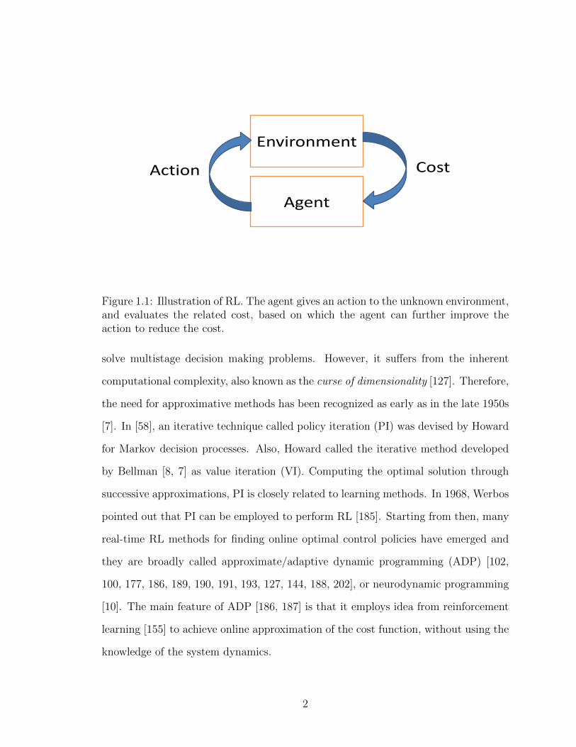
be achieved (see Figure 1.1). The definition of RL can be quite general. Indeed,
the well-known trial-and-error method can be considered as one simple scheme of
reinforcement learning, because trial-and-error, together with delayed reward [181],
are two important features of RL [155]. In the seminal book by Sutton and Barto
[155], the RL problem is referred to as how to map situations to actions so as to
minimize a numerical reward signal. As an important branch in machine learning
theory, RL has been brought to the computer science and control science literature as
a way to study artificial intelligence in the 1960s [115, 117, 176]. Since then, numerous
contributions to RL, from a control perspective, have been made (see, for example,
[5, 154, 181, 102, 103, 174, 88]).
On the other hand, Dynamic programming (DP) [8] offers a theoretical way to
1
Cost
Environment
Agent
Action
Figure 1.1: Illustration of RL. The agent gives an action to the unknown environment,and evaluates the related cost, based on which the agent can further improve theaction to reduce the cost.
solve multistage decision making problems. However, it suffers from the inherent
computational complexity, also known as the curse of dimensionality [127]. Therefore,
the need for approximative methods has been recognized as early as in the late 1950s
[7]. In [58], an iterative technique called policy iteration (PI) was devised by Howard
for Markov decision processes. Also, Howard called the iterative method developed
by Bellman [8, 7] as value iteration (VI). Computing the optimal solution through
successive approximations, PI is closely related to learning methods. In 1968, Werbos
pointed out that PI can be employed to perform RL [185]. Starting from then, many
real-time RL methods for finding online optimal control policies have emerged and
they are broadly called approximate/adaptive dynamic programming (ADP) [102,
100, 177, 186, 189, 190, 191, 193, 127, 144, 188, 202], or neurodynamic programming
[10]. The main feature of ADP [186, 187] is that it employs idea from reinforcement
learning [155] to achieve online approximation of the cost function, without using the
knowledge of the system dynamics.
2

1.1.2 The development of ADP
The development of ADP theory consists of three phases. In the first phase, ADP was
extensively investigated within the communities of computer science and operations
research. Two basic algorithms, policy iteration [58] and value iteration [8], are
usually employed. In [154], Sutton introduced the temporal difference method. In
1989, Watkins proposed the well-known Q-learning method in his PhD thesis [181].
Q-learning shares similar features with the action-dependent HDP scheme proposed
by Werbos in [189]. Other related research work under a discrete time and discrete
state-space Markov decision process framework can be found in [11, 10, 18, 23, 127,
130, 156, 155] and references therein. In the second phase, stability is brought into the
context of ADP while real-time control problems are studied for dynamic systems.
To the best of the author’s knowledge, Lewis is the first who contributes to the
integration of stability theory and ADP theory [102]. An essential advantage of ADP
theory is that an optimal control policy can be obtained via a recursive numerical
algorithm using online information without solving the HJB equation (for nonlinear
systems) and the algebraic Riccati equation (ARE) (for linear systems), even when
the system dynamics are not precisely known. Optimal feedback control designs for
linear and nonlinear dynamic systems have been proposed by several researchers over
the past few years; see, e.g., [12, 34, 118, 122, 167, 173, 196, 203]. While most of the
previous work on ADP theory was devoted to discrete-time (DT) systems (see [100]
and references therein), there has been relatively less research for the continuous-time
(CT) counterpart. This is mainly because ADP is considerably more difficult for CT
systems than for DT systems. Indeed, many results developed for DT systems [107]
cannot be extended straightforwardly to CT systems. Nonetheless, early attempts
were made to apply Q-learning for CT systems via discretization technique [4, 35].
However, convergence and stability analysis of these schemes are challenging. In [122],
Murray et. al proposed an implementation method which requires the measurements
3
of the derivatives of the state variables. As said previously, Lewis and his co-worker
proposed the first solution to stability analysis and convergence proofs for ADP-based
control systems by means of LQR theory [173]. A synchronous policy iteration scheme
was also presented in [166]. For CT linear systems, the partial knowledge of the system
dynamics (i.e., the input matrix) must be precisely known. This restriction has been
completely removed in [68]. A nonlinear variant of this method can be found in [75].
The third phase in the development of ADP theory is related to extensions of
previous ADP results to nonlinear uncertain systems. Neural networks and game
theory are utilized to address the presence of uncertainty and nonlinearity in control
systems. See, e.g. [51, 167, 168, 203, 100, 198, 204, 183]. An implicit assumption in
these papers is that the system order is known and that the uncertainty is static, not
dynamic. The presence of dynamic uncertainty has not been systematically addressed
in the literature of ADP. By dynamic uncertainty, we refer to the mismatch between
the nominal model and the real plant when the order of the nominal model is lower
than the order of the real system. A closely related topic of research is how to
account for the effect of unseen variables [188]. It is quite common that the full-state
information is often missing in many engineering applications and only the output
measurement or partial-state measurements are available. Adaptation of the existing
ADP theory to this practical scenario is important yet non-trivial. Neural networks
are sought for addressing the state estimation problem [37, 87]. However, the stability
analysis of the estimator/controller augmented system is by no means easy, because
the total system is highly interconnected. The configuration of a standard ADP-based
control system is shown in Figure 1.2.
Our recent work [67, 73, 70, 67, 69] on the development of robust ADP (for short,
RADP) theory is exactly targeted at addressing these challenges.
4
Control action
Environment
Critic
Actor
State/output
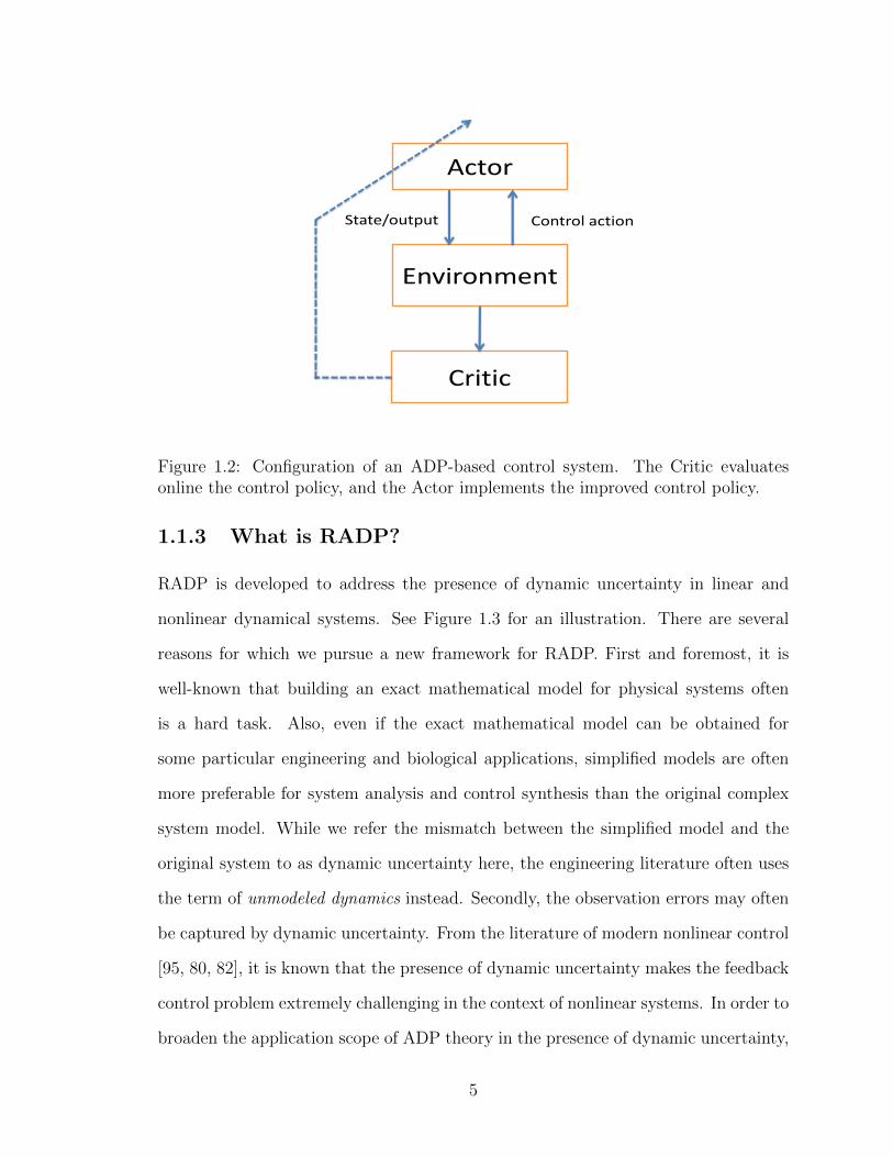
Figure 1.2: Configuration of an ADP-based control system. The Critic evaluatesonline the control policy, and the Actor implements the improved control policy.
1.1.3 What is RADP?
RADP is developed to address the presence of dynamic uncertainty in linear and
nonlinear dynamical systems. See Figure 1.3 for an illustration. There are several
reasons for which we pursue a new framework for RADP. First and foremost, it is
well-known that building an exact mathematical model for physical systems often
is a hard task. Also, even if the exact mathematical model can be obtained for
some particular engineering and biological applications, simplified models are often
more preferable for system analysis and control synthesis than the original complex
system model. While we refer the mismatch between the simplified model and the
original system to as dynamic uncertainty here, the engineering literature often uses
the term of unmodeled dynamics instead. Secondly, the observation errors may often
be captured by dynamic uncertainty. From the literature of modern nonlinear control
[95, 80, 82], it is known that the presence of dynamic uncertainty makes the feedback
control problem extremely challenging in the context of nonlinear systems. In order to
broaden the application scope of ADP theory in the presence of dynamic uncertainty,
5
Control action
Environment
Critic
Actor
State/output
Dynamic Uncertainties
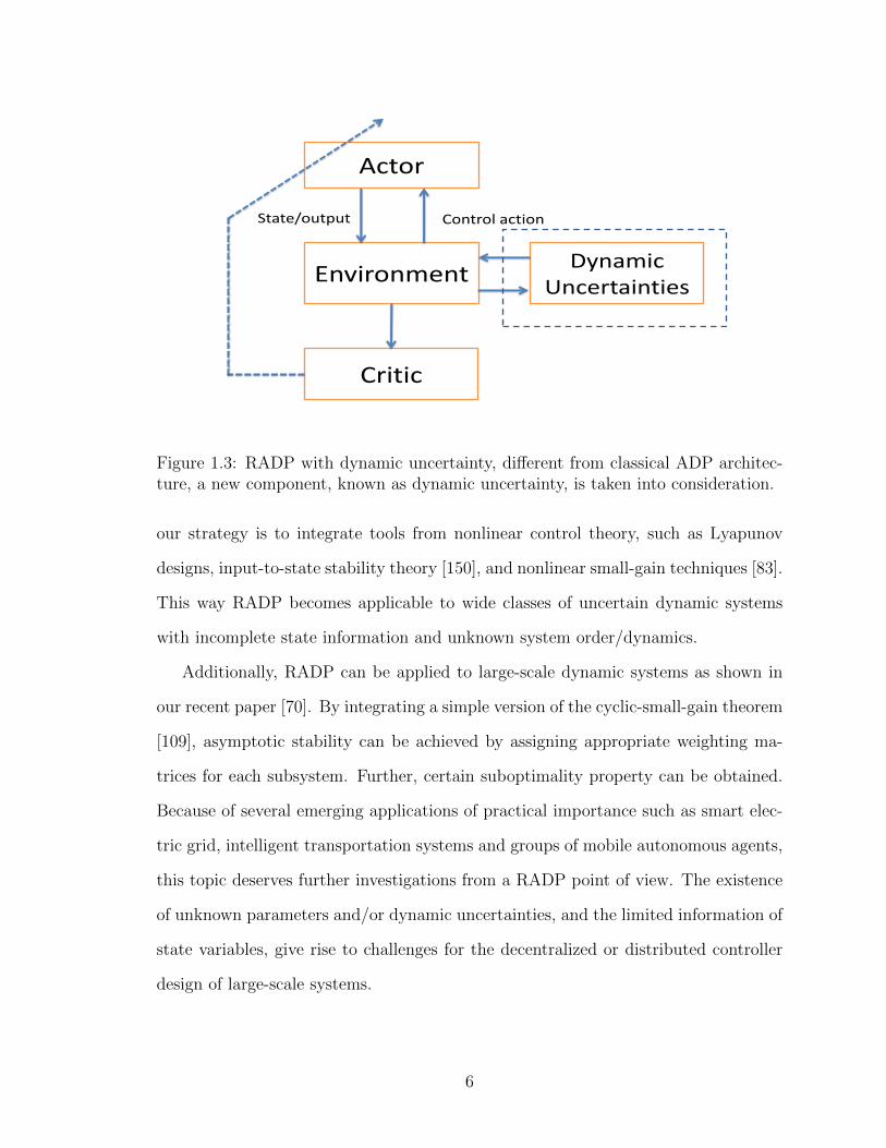
Figure 1.3: RADP with dynamic uncertainty, different from classical ADP architec-ture, a new component, known as dynamic uncertainty, is taken into consideration.
our strategy is to integrate tools from nonlinear control theory, such as Lyapunov
designs, input-to-state stability theory [150], and nonlinear small-gain techniques [83].
This way RADP becomes applicable to wide classes of uncertain dynamic systems
with incomplete state information and unknown system order/dynamics.
Additionally, RADP can be applied to large-scale dynamic systems as shown in
our recent paper [70]. By integrating a simple version of the cyclic-small-gain theorem
[109], asymptotic stability can be achieved by assigning appropriate weighting ma-
trices for each subsystem. Further, certain suboptimality property can be obtained.
Because of several emerging applications of practical importance such as smart elec-
tric grid, intelligent transportation systems and groups of mobile autonomous agents,
this topic deserves further investigations from a RADP point of view. The existence
of unknown parameters and/or dynamic uncertainties, and the limited information of
state variables, give rise to challenges for the decentralized or distributed controller
design of large-scale systems.
6
1.2 Contributions of this dissertation
Here we outline the key contributions of the dissertation as follows.
• We, for the first time, develop ADP methods for CT systems with completely
unknown dynamics.
– By taking advantages of the exploration noise, we remove the assumption in
the past literature of ADP where partial knowledge of the system dynamics
must be known [68].
– We extend the method to affine nonlinear systems and rigorously show its
stability and convergence properties [75].
– We introduce sum-of-squares-based relaxation method into ADP theory to
achieve global stabilization and suboptimal control of uncertain nonlinear
systems via online learning [71].
• We propose the new theory of RADP, which fills a gap of ADP in the past liter-
ature where dynamic uncertainties or unmodeled dynamics are not addressed.
– Inspired by the small-gain theorem [83], for partially linear systems, we
give conditions on the design of the performance index to achieve robust
stability [69].
– We extend this technique to a class of large-scale systems [70].
– By integration with tools from nonlinear control theory, e.g., gain-assignment
[129], and the Lyapunov-based small-gain condition [81], we redesign the
approximated optimal controller to achieve robust stabilization of nonlin-
ear system with dynamic uncertainties [75].
• We have applied the RADP theory to study both engineering and reverse-
engineering problems.
7
– The RADP theory is used to study the robust optimal control of multima-
chine power systems [70, 73].
– Observing good consistency between experimental data [22, 41, 142] and
our simulation results, we suggest that biological systems may use RADP-
like schemes to interact with uncertain environment [74, 76].
8
Chapter 2
ADP for linear systems with
completely unknown dynamics
The adaptive controller design for unknown linear systems has been intensively stud-
ied in the past literature [60], [113], [158]. A conventional way to design an adaptive
optimal control law can be pursued by identifying the system parameters first and
then solving the related algebraic Riccati equation. However, adaptive systems de-
signed this way are known to respond slowly to parameter variations from the plant.
On the other hand, approximate/adaptive dynamic programming (ADP) [186]
theories have been broadly applied for solving optimal control problems for uncertain
systems in recent years (see, for example, [102, 177, 38, 2, 12, 34, 196, 66, 101, 173,
203, 192]). Among all the different ADP approaches, for discrete-time (DT) systems,
the action-dependent heuristic dynamic programming (ADHDP) [189], or Q-learning
[181], is an online iterative scheme that does not depend on the model to be controlled,
and it has found applications in many engineering disciplines [1, 196, 101, 184].
Nevertheless, due to the different structures of the algebraic Riccati equations
between DT and continuous-time (CT) systems, results developed for the DT setting
cannot be directly applied for solving CT problems. Although some early attempts
9
have been made in [4, 122, 173], a common feature of all the existing ADP-based
results is that partial knowledge of the system dynamics is assumed to be exactly
known in the setting of CT systems.
The primary objective of this chapter is to remove this assumption on partial
knowledge of the system dynamics, and thus to develop a truly knowledge-free AD-
P algorithm. More specifically, we propose a novel computational adaptive optimal
control methodology that employs the approximate/adaptive dynamic programming
technique to iteratively solve the algebraic Riccati equation using the online infor-
mation of state and input, without requiring the a priori knowledge of the system
matrices. In addition, all iterations can be conducted by using repeatedly the same s-
tate and input information on some fixed time intervals. It should be noticed that our
approach serves as a fundamental computational tool to study ADP related problems
for CT systems in the remainder of this dissertation.
This Chapter is organized as follows: In Section 2.1, we briefly introduce a policy
iteration technique for solving standard CT linear systems. In Section 2.2, we de-
velop our computational adaptive optimal control method and show its convergence.
A practical online algorithm is provided. In Section 2.3, we apply the proposed ap-
proach to the optimal controller design problem of a turbocharged diesel engine with
exhaust gas recirculation. Concluding remarks as well as potential future extensions
are contained in Section 2.4.
2.1 Problem formulation and preliminaries
Consider a CT linear system described by
x = Ax+Bu (2.1)
10
where x ∈ Rn is the system state fully available for feedback control design; u ∈ Rm
is the control input; A ∈ Rn×n and B ∈ Rn×m are unknown constant matrices. In
addition, the system is assumed to be stabilizable.
Recall the LQR design mentioned in Section 9.1.1. The design objective is to find
a linear optimal control law in the form of
u = −Kx (2.2)
which minimizes the following performance index
J =
∫ ∞
0
(xTQx+ uTRu)dt (2.3)
where Q = QT ≥ 0, R = RT > 0, with (A,Q1/2) observable.
By [99], solution to this problem can be found by solving the following well-known
algebraic Riccati equation (ARE)
ATP + PA+Q− PBR−1BTP = 0, (2.4)
which has a unique symmetric positive definite solution P ∗. Then, the optimal feed-
back gain matrix K∗ in (2.2) is thus determined by
K∗ = R−1BTP ∗. (2.5)
Since (2.4) is nonlinear in P , it is usually difficult to directly solve P ∗ from (2.4),
especially for large-size matrices. Nevertheless, many efficient algorithms have been
developed to numerically approximate the solution of (2.4). One of such algorithms
was developed in [89], and is introduced in the following:
Theorem 2.1.1 ([89]). Let K0 ∈ Rm×n be any stabilizing feedback gain matrix, and
11
let Pk be the real symmetric positive definite solution of the Lyapunov equation
(A−BKk)T Pk + Pk (A−BKk) +Q+KT
k RKk = 0 (2.6)
where Kk, with k = 1, 2, · · · , are defined recursively by:
Kk = R−1BTPk−1. (2.7)
Then, the following properties hold:
1. A−BKk is Hurwitz,
2. P ∗ ≤ Pk+1 ≤ Pk,
3. limk→∞
Kk = K∗, limk→∞
Pk = P ∗.
In [89], by iteratively solving the Lyapunov equation (2.6), which is linear in Pk,
and updating Kk by (2.7), solution to the nonlinear equation (2.4) is numerically
approximated.
For the purpose of solving (2.6) without the knowledge of A, in [173], (2.6) was
implemented online by
xT (t)Pkx(t)− xT (t+ δt)Pkx(t+ δt) =
∫ t+δt
t
(xTQx+ uTkRuk
)dτ (2.8)
where uk = −Kkx is the control input of the system on the time interval [t, t+ δt].
Since both x and uk can be measured online, a real symmetric solution Pk can be
uniquely determined under certain persistent excitation (PE) condition [173]. Howev-
er, as we can see from (2.7), the exact knowledge of system matrix B is still required
for the iterations. Also, to guarantee the PE condition, the state may need to be reset
at each iteration step, but this may cause technical problems for stability analysis of
the closed loop system [173]. An alternative way is to add exploration noise [19],
12
[167], [1], [196] such that uk = −Kkx+ e, with e the exploration noise, is used as the
true control input in (2.8). As a result, Pk solved from (2.8) and the one solved from
(2.6) are not exactly the same. In addition, after each time the control policy is up-
dated, information of the state and input must be re-collected for the next iteration.
This may slow down the learning process, especially for high-dimensional systems.
2.2 ADP-based online learning with completely un-
known dynamics
In this section, we will present our new online learning strategy that does not rely on
A nor B.
To this end, we rewrite the original system (2.1) as
x = Akx+B(Kkx+ u) (2.9)
where Ak = A−BKk.
Then, along the solutions of (2.9), by (2.6) and (2.7) it follows that
x(t+ δt)TPkx(t+ δt)− x(t)TPkx(t)
=
∫ t+δt
t
[xT (ATkPk + PkAk)x+ 2(u+Kkx)TBTPkx
]dτ (2.10)
= −∫ t+δt
t
xTQkx dτ + 2
∫ t+δt
t
(u+Kkx)TRKk+1x dτ
where Qk = Q+KTk RKk.
Remark 2.2.1. Notice that in (2.10), the term xT (ATkPk + PkAk)x depending on
the unknown matrices A and B is replaced by −xTQkx, which can be obtained by
measuring the state online. Also, the term BTPk involving B is replaced by RKk+1,
in which Kk+1 is treated as another unknown matrix to be solved together with Pk.
13
Therefore, (2.10) plays an important role in separating the system dynamics from the
iterative process. As a result, the requirement of the system matrices in (2.6) and
(2.7) can be replaced by the state and input information measured online.
Remark 2.2.2. It is also noteworthy that in (2.10) we always have exact equality
if Pk, Kk+1 satisfy (2.6), (2.7), and x is the solution of system (2.9) with arbitrary
control input u. This fact enables us to employ u = −K0x+ e, with e the exploration
noise, as the input signal for learning, without affecting the convergence of the learning
process.
Next, we show that given a stabilizing Kk, a pair of matrices (Pk, Kk+1), with
Pk = P Tk > 0, satisfying (2.6) and (2.7) can be uniquely determined without knowing
A or B , under certain condition. To this end, we define the following two operators:
ν(P ) : Rn×n → R12n(n+1), and µ(x) : Rn → R
12n(n+1)
such that
ν(P ) = [p11, 2p12, · · · , 2p1n, p22, 2p23, · · · , 2pn−1,n, pnn]T ,
µ(x) = [x21, x1x2, · · · , x1xn, x
22, x2x3, · · · , xn−1xn, x
2n]T .
In addition, by Kronecker product representation, we have
xTQkx =(xT ⊗ xT
)vec(Qk),
and
(u+Kkx)TRKk+1x
=[(xT ⊗ xT )(In ⊗KT
k R) + (xT ⊗ uT ) (In ⊗R)]
vec(Kk+1).
14
Further, for positive integer l, we define matrices δxx ∈ Rl× 12n(n+1), Ixx ∈ Rl×n2
,
Ixu ∈ Rl×mn, such that
δxx =
[µ(x(t1))− µ(x(t0)), µ(x(t2))− µ(x(t1)), · · · , µ(x(tl))− µ(x(tl−1))
]T,
Ixx =
[ ∫ t1t0x⊗ x dτ,
∫ t2t1x⊗ x dτ, · · · ,
∫ tltl−1
x⊗ x dτ]T,
Ixu =
[ ∫ t1t0x⊗ u dτ,
∫ t2t1x⊗ u dτ, · · · ,
∫ tltl−1
x⊗ u dτ]T,
where 0 ≤ t0 < t1 < · · · < tl.
Then, for any given stabilizing gain matrix Kk, (2.10) implies the following matrix
form of linear equations
Θk
ν(Pk)
vec (Kk+1)
= Ξk (2.11)
where Θk ∈ Rl×[ 12n(n+1)+mn] and Ξk ∈ Rl are defined as:
Θk =[δxx,−2Ixx(In ⊗KT
k R)− 2Ixu(In ⊗R)],
Ξk = −Ixx vec(Qk).
Notice that if Θk has full column rank, (2.11) can be directly solved as follows:
ν(Pk)
vec (Kk+1)
= (ΘT
kΘk)−1ΘT
kΞk. (2.12)
Now, we are ready to give the following computational adaptive optimal control
algorithm for practical online implementation. A flowchart of Algorithm 2.2.1 is
shown in Figure 2.1.
Remark 2.2.3. Computing the matrices Ixx and Ixu carries the main burden in
15

Algorithm 2.2.1 ADP algorithm
1: Employ u = −K0x + e as the input on the time interval [t0, tl], where K0 isstabilizing and e is the exploration noise. Compute δxx, Ixx and Ixu until the rankcondition in (2.13) below is satisfied. Let k = 0.
2: Solve Pk and Kk+1 from (2.12).3: Let k ← k + 1, and repeat Step 2 until ‖Pk − Pk−1‖ ≤ ε for k ≥ 1, where the
constant ε > 0 is a predefined small threshold.4: Use u = −Kkx as the approximated optimal control policy.
StartInitialization: k = 0and K0 is stabilizing.
Let u = −K0x + e, t ∈[t0, tl], and computeδxx, Ixx, and Ixu.
Solve Pk and Kk+1 from[Pk
vec(Kk+1)
]=(ΘT
k Θk
)−1ΘT
k Ξk.
‖Pk−Pk−1‖ ≤ε for k ≥ 1
Use u = −Kkx asthe control input.
Stop
k ← k+ 1
Yes
No
1Figure 2.1: Flowchart of Algorithm 2.2.1.
performing Algorithm 2.2.1. The two matrices can be implemented using 12n(n+ 1) +
mn integrators in the learning system to collect information of the state and the input.
Remark 2.2.4. In practice, numerical error may occur when computing Ixx and Ixu.
As a result, the solution of (2.11) may not exist. In that case, the solution of (2.12)
can be viewed as the least squares solution of (2.11).
Next, we show that the convergence of Algorithm 2.2.1 can be guaranteed under
certain condition.
16

Lemma 2.2.1. If there exists an integer l0 > 0, such that, for all l ≥ l0,
rank
([Ixx, Ixu
])=n(n+ 1)
2+mn, (2.13)
then Θk has full column rank for all k ∈ Z+.
Proof: It amounts to show that the following linear equation
ΘkX = 0 (2.14)
has only the trivial solution X = 0.
To this end, we prove by contradiction. AssumeX =
[Y Tv ZT
v
]T∈ R 1
2n(n+1)+mn
is a nonzero solution of (2.14), where Yv ∈ R 12n(n+1) and Zv ∈ Rmn. Then, a symmetric
matrix Y ∈ Rn×n and a matrix Z ∈ Rm×n can be uniquely determined, such that
ν(Y ) = Yv and vec(Z) = Zv.
By (2.10), we have
ΘkX = Ixxvec(M) + 2Ixuvec(N) (2.15)
where
M = ATk Y + Y Ak +KTk (BTY −RZ) + (Y B − ZTR)Kk, (2.16)
N = BTY −RZ. (2.17)
Notice that since M is symmetric, we have
Ixxvec(M) = Ixν(M) (2.18)
17
where Ix ∈ Rl× 12n(n+1) is defined as:
Ix =
[ ∫ t1t0µ(x)dτ,
∫ t2t1µ(x)dτ, · · · ,
∫ tltl−1
µ(x)dτ
]T. (2.19)
Then, (2.14) and (2.15) imply the following matrix form of linear equations
[Ix, 2Ixu
]
ν(M)
vec(N)
= 0. (2.20)
Under the rank condition in (2.13), we know
[Ix, 2Ixu
]has full column rank.
Therefore, the only solution to (2.20) is ν(M) = 0 and vec(N) = 0. As a result, we
have M = 0 and N = 0.
Now, by (2.17) we know Z = R−1BTY , and (2.16) is reduced to the following
Lyapunov equation
ATk Y + Y Ak = 0. (2.21)
Since Ak is Hurwitz for all k ∈ Z+, the only solution to (2.21) is Y = 0. Finally, by
(2.17) we have Z = 0.
In summary, we have X = 0. But it contradicts with the assumption that X 6= 0.
Therefore, Θk must have full column rank for all k ∈ Z+. The proof is complete.
Theorem 2.2.1. Starting from a stabilizing K0 ∈ Rm×n, when the condition of Lem-
ma 2.2.1 is satisfied, the sequences Pi∞i=0 and Kj∞j=1 obtained from solving (2.12)
converge to the optimal values P ∗ and K∗, respectively.
Proof: Given a stabilizing feedback gain matrix Kk, if Pk = P Tk is the solution of
(2.6), Kk+1 is uniquely determined by Kk+1 = R−1BTPk. By (2.10), we know that
Pk and Kk+1 satisfy (2.12). On the other hand, let P = P T ∈ Rn×n and K ∈ Rm×n,
18
such that
Θk
ν(P )
vec(K)
= Ξk.
Then, we immediately have ν(P ) = ν(Pk) and vec(K) = vec(Kk+1). By Lemma
2.2.1, P = P T and K are unique. In addition, by the definitions of ν(P ) and vec(K),
Pk = P and Kk+1 = K are uniquely determined.
Therefore, the policy iteration (2.12) is equivalent to (2.6) and (2.7). By Theorem
2.1.1, the convergence is thus proved.
Remark 2.2.5. It can be seen that Algorithm 2.2.1 contains two separated phases:
First, an initial stabilizing control policy with exploration noise is applied and the
online information is recorded in matrices δxx, Ixx, and Ixu until the rank condition
in (2.13) is satisfied. Second, without requiring additional system information, the
matrices δxx, Ixx, and Ixu are repeatedly used to implement the iterative process. A
sequence of controllers, that converges to the optimal control policy, can be obtained.
Remark 2.2.6. The choice of exploration noise is not a trivial task for general rein-
forcement learning problems and other related machine learning problems, especially
for high dimensional systems. In solving practical problems, several types of explo-
ration noise have been adopted, such as random noise [1], [196], exponentially de-
creasing probing noise [167]. For the simulations in the next section, we will use the
sum of sinusoidal signals with different frequencies, as in [69].
Remark 2.2.7. In some sense, our approach is related to the ADHDP [189], or Q-
learning [181] method for DT systems. Indeed, it can be viewed that we solve the
following matrix Hk at each iteration step
Hk =
H11,k H12,k
H21,k H22,k
=
Pk PkB
BTPk R
. (2.22)
19

Once this matrix is obtained, the control policy can be updated by Kk+1 = H−122,kH21,k.
The DT version of the Hk matrix can be found in [19] and [102].
2.3 Application to a turbocharged diesel engine
In this section, we study the controller design for a turbocharged diesel engine with
exhaust gas recirculation [84]. The open loop model is a six-th order CT linear system.
The system matrices A and B are directly taken from [84] and shown as follows:
A =
−0.4125 −0.0248 0.0741 0.0089 0 0
101.5873 −7.2651 2.7608 2.8068 0 0
0.0704 0.0085 −0.0741 −0.0089 0 0.0200
0.0878 0.2672 0 −0.3674 0.0044 0.3962
−1.8414 0.0990 0 0 −0.0343 −0.0330
0 0 0 −359.0000 187.5364 −87.0316
,
B =
−0.0042 −1.0360 0.0042 0.1261 0 0
0.0064 1.5849 0 0 −0.0168 0
T
.
In order to illustrate the efficiency of the proposed computational adaptive optimal
control strategy, the precise knowledge of A and B is not used in the design of optimal
controllers. Since the physical system is already stable, the initial stabilizing feedback
gain can be set as K0 = 0.
The weighting matrices are selected to be
Q = diag
(1, 1, 0.1, 0.1, 0.1, 0.1
), R = I2.
In the simulation, the initial values for the state variables are randomly selected
around the origin. From t = 0s to t = 2s, the following exploration noise is used as
20

0 50 100 150 200−50
0
50
100
150
200
Time (sec)
||x||
Figure 2.2: Trajectory of the Euclidean norm of the state variables during the simu-lation.
the system input
e = 100100∑
i=1
sin(ωit) (2.23)
where ωi, with i = 1, · · · , 100, are randomly selected from [−500, 500].
State and input information is collected over each interval of 0.01s. The policy
iteration started at t = 2s, and convergence is attained after 16 iterations, when the
stopping criterion ‖Pk − Pk−1‖ ≤ 0.03 is satisfied. The formulated controller is used
as the actual control input to the system starting from t = 2s to the end of the
simulation. The trajectory of the Euclidean norm of all the state variables is shown
in Figure 2.2. The system output variables y1 = 3.6x6 and y2 = x4, denoting the mass
air flow (MAF) and the intake manifold absolute pressure (MAP) [84], are plotted in
Figure 2.3.
21
0 1 2 3 4 5 6 7 8 9 10−80
−60
−40
−20
0
20
40
Time (sec)
y
1 (MAF)
y2 (MAP)
Control policy updated
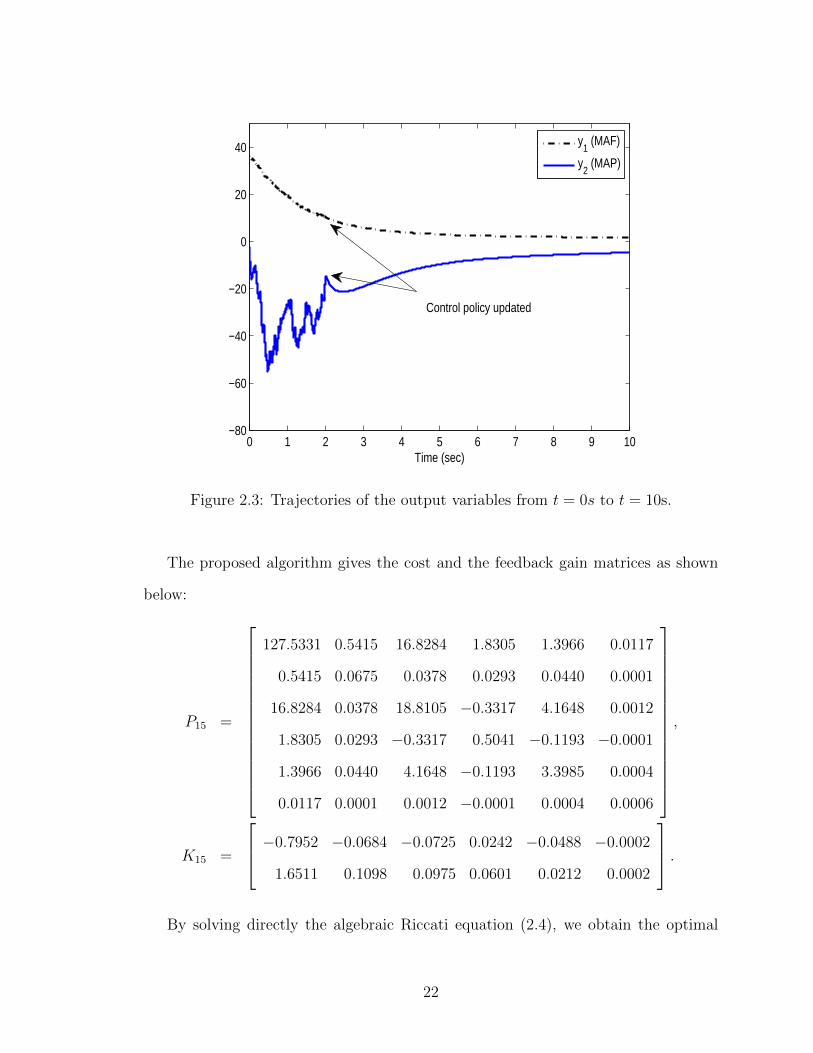
Figure 2.3: Trajectories of the output variables from t = 0s to t = 10s.
The proposed algorithm gives the cost and the feedback gain matrices as shown
below:
P15 =
127.5331 0.5415 16.8284 1.8305 1.3966 0.0117
0.5415 0.0675 0.0378 0.0293 0.0440 0.0001
16.8284 0.0378 18.8105 −0.3317 4.1648 0.0012
1.8305 0.0293 −0.3317 0.5041 −0.1193 −0.0001
1.3966 0.0440 4.1648 −0.1193 3.3985 0.0004
0.0117 0.0001 0.0012 −0.0001 0.0004 0.0006
,
K15 =
−0.7952 −0.0684 −0.0725 0.0242 −0.0488 −0.0002
1.6511 0.1098 0.0975 0.0601 0.0212 0.0002
.
By solving directly the algebraic Riccati equation (2.4), we obtain the optimal
22
0 5 10 15−5
0
5
10
15
Number of iterations
0 5 10 15−0.5
0
0.5
1
1.5
2
Number of iterations
||Pk−P*||
||Kk−K*||
Figure 2.4: Convergence of Pk and Kk to their optimal values P ∗ and K∗ during thelearning process.
23
solutions:
P ∗ =
127.5325 0.5416 16.8300 1.8307 1.4004 0.0117
0.5416 0.0675 0.0376 0.0292 0.0436 0.0001
16.8300 0.0376 18.8063 −0.3323 4.1558 0.0012
1.8307 0.0292 −0.3323 0.5039 −0.1209 −0.0001
1.4004 0.0436 4.1558 −0.1209 3.3764 0.0004
0.0117 0.0001 0.0012 −0.0001 0.0004 0.0006
,
K∗ =
−0.7952 −0.0684 −0.0726 0.0242 −0.0488 −0.0002
1.6511 0.1098 0.0975 0.0601 0.0213 0.0002
.
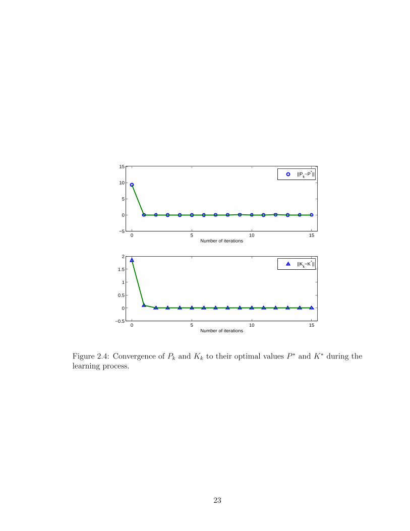
The convergence of Pk and Kk to their optimal values is illustrated in Figure
2.4. Notice that if B is accurately known, the problem can also be solved using the
method in [173]. However, that method requires a total learning time of 32s for 16
iterations, if the state and input information within 2s is collected for each iteration.
In addition, the method in [173] may need to reset the state at each iteration step,
in order to satisfy the PE condition.
2.4 Conclusions
A novel computational policy iteration approach for finding online adaptive optimal
controllers for CT linear systems with completely unknown system dynamics has
been presented in this chapter. This method solves the algebraic Riccati equation
iteratively using system state and input information collected online, without knowing
the system matrices. A practical online algorithm was proposed and has been applied
to the controller design for a turbocharged diesel engine with unknown parameters.
The methodology developed in this chapter serves as an important computational tool
to study the adaptive optimal control of CT systems. It is essential to the theories
24

developed in the remaining chapters of this dissertation.
25
Chapter 3
RADP for uncertain partially
linear systems
In the previous chapter, we have developed an ADP methodology for CT linear sys-
tems. Similar to the past literature of ADP, it is assumed that the system order is
known and the state variables are fully available. However, the system order may be
unknown due to the presence of dynamic uncertainties (or unmodeled dynamics) [82],
which are motivated by engineering applications in situations where the exact math-
ematical model of a physical system is not easy to be obtained. Of course, dynamic
uncertainties also make sense for the mathematical modeling in other branches of sci-
ence such as biology and economics. This problem, often formulated in the context of
robust control theory, cannot be viewed as a special case of output feedback control.
In addition, the ADP methods developed in the past literature may fail to guarantee
not only optimality, but also the stability of the closed-loop system when dynamic
uncertainty occurs. In the seminal paper [192], Werbos also pointed out the related
issue that the performance of learning may deteriorate when using incomplete data
in ADP.
In order to capture and model this feature from biological learning, in this chap-
26

ter we propose a new concept of robust adaptive dynamic programming, a natural
extension of ADP to uncertain dynamic systems. It is worth noting that we focus
on the presence of dynamic uncertainties of which the state variables and the system
order are not precisely known.
As the first distinctive feature of the proposed RADP framework, the controller
design issue is addressed from a point of view of robust control with disturbance
attenuation. Specifically, by means of the popular backstepping approach [95], we
will show that a robust control policy, or adaptive critic, can be synthesized to yield
an arbitrarily small L2-gain with respect to the disturbance input. In addition, by
studying the relationship between optimality and robustness, it is shown that in the
absence of disturbance input, the robust control policy also preserves optimality with
respect to some iteratively constructed cost function. It should be mentioned that in
[1] the theory of zero-sum games was employed in ADP design but the gain from the
disturbance input to the output cannot be made arbitrarily small.
Our study on the effects of dynamic uncertainties, or unmodeled dynamics, is
motivated by engineering applications in situations where the exact mathematical
model of a physical system is not easy to be obtained. The presence of dynamic
uncertainty gives rise to interconnected systems for which the controller design and
robustness analysis become technically challenging. With this observation in mind,
we will adopt notions of input-to-output stability and strong unboundedness observ-
ability introduced in the nonlinear control community; see, for instance, [61, 83], and
[150]. We achieve the robust stability and suboptimality properties for the overall
interconnected system, by means of Lyapunov and small-gain techniques [83].
This chapter is organized as follows. Section 3.1 formulates the problem. Section
3.2 investigates the relationship between optimality and robustness for a general class
of partially linear, uncertain composite systems [133]. Section 3.3 presents a RAD-
P scheme for partial-state feedback design. Section 3.4 demonstrates the proposed
27

RADP design methodology by means of an one-machine infinite-bus power system.
Concluding remarks are contained in Section 3.5.
3.1 Problem formulation
Consider the following partially linear composite system
w = f(w, y), (3.1)
x = Ax+B [z + ∆1(w, y)] , (3.2)
z = Ex+ Fz +G [u+ ∆2(w, y)] , (3.3)
y = Cx (3.4)
where [xT , zT ]T ∈ Rn × Rm is the system state vector; w ∈ Rnw is the state of the
dynamic uncertainty; y ∈ Rq is the output; u ∈ Rm is the control input; A ∈ Rn×n,
B ∈ Rn×m, C ∈ Rq×n, E ∈ Rm×n, F ∈ Rm×m, and G ∈ Rm×m are unknown constant
matrices with the pair (A,B) stabilizable and G nonsingular; ∆1(w, y) = D∆(w, y)
and ∆2(w, y) = H∆(w, y) are the outputs of the dynamic uncertainty with D,H ∈
Rm×p two unknown constant matrices; the unknown functions f : Rnw × Rq → Rnw
and ∆ : Rnw × Rq → Rp are locally Lipschitz satisfying f(0, 0) = 0, ∆(0, 0) = 0. In
addition, assume the upper bounds of the norms of B, D, H, and G−1 are known.
Our objective is to find online a robust optimal control policy that globally asymp-
totically stabilizes the system (3.1)-(3.4) at the origin.
3.2 Optimality and robustness
In this section, we show the existence of a robust optimal control policy that globally
asymptotically stabilizes the overall system (3.1)-(3.4). To this end, let us make a few
assumptions on (3.1), which are often required in the literature of nonlinear control
28
design [61, 82, 95].
Assumption 3.2.1. The w-subsystem (3.1) has strong unboundedness observability
(SUO) property with zero offset [83] and is input-to-output stable (IOS) with respect
to y as the input and ∆ as the output [83, 150].
Assumption 3.2.2. There exist a continuously differentiable, positive definite, radi-
ally unbounded function U : Rnw → R+, and a constant c ≥ 0 such that
U =∂U(w)
∂wf(w, y) ≤ −2|∆|2 + c|y|2 (3.5)
for all w ∈ Rnw and y ∈ Rq.
We now show that an arbitrarily small L2 gain can be obtained for the subsystem
(3.2)-(3.4). Given any arbitrarily small constant γ > 0, we can choose Q and R in
(3.15) such that Q ≥ γ−1CTC and R−1 ≥ DDT . Define K∗ = R−1BTP ∗, ξ = z+K∗x,
Ac = A−BK∗, and let S∗ > 0 be the symmetric solution of the ARE
F TS∗ + S∗F +W − S∗GR−11 GTS∗ = 0 (3.6)
where W > 0, R−11 ≥ DDT , F = F +K∗B, and D = H+G−1K∗BD. Further, define
E = E +K∗Ac − FK∗, M∗ = R−11 GTS∗, N∗ = S∗E.
The following theorem gives the small-gain condition for the robust asymptotic
stability of the overall system (3.1)-(3.4).
Theorem 3.2.1. Under Assumptions 3.2.1 and 3.2.2, the control policy
u∗ = −[(M∗TR1)−1(N∗ +RK∗) +M∗K∗
]x−M∗z (3.7)
globally asymptotically stabilizes the closed-loop system comprised of (3.1)-(3.4), if
29
the small-gain condition holds:
γc < 1. (3.8)
Proof. Define
V (x, z, w) = xTP ∗x+ ξTS∗ξ + U (w) . (3.9)
Then, along the solutions of the closed-loop system comprised of (3.1)-(3.4) and (3.7),
by completing squares, it follows that
V =d
dt(xTP ∗x) +
d
dt(ξTS∗ξ) + U
≤ −γ−1|y|2 + |∆|2 + 2xTP ∗Bξ + |∆|2
−2ξTBTP ∗x+(c|y|2 − 2|∆|2
)
≤ −γ−1(1− cγ)|y|2
Therefore, we know limt→∞
y(t) = 0. By Assumption 3.2.1, all solutions of the
closed-loop system are globally bounded. Moreover, a direct application of LaSalle’s
Invariance Principle [86] yields the GAS property of the trivial solution of the closed-
loop system.
The proof is thus complete.
Next, we show that the control policy (3.7) is suboptimal, i.e., it is optimal with
respect to some cost function in the absence of the dynamic uncertainty. Notice that,
with ∆ ≡ 0, the system (3.2)-(3.3) can be rewritten in a more compact matrix form:
X = A1X +G1v (3.10)
where X =
xT
ξT
, v = u+G−1
[E + (S∗)−1BTP ∗
]x, A1 =
Ac B
−(S∗)−1BTP ∗ F
,
30

and G1 =
0
G
.
Proposition 3.2.1. Under the conditions of Theorem 3.2.1, the performance index
J1 =
∫ ∞
0
[XTQ1X + vTR1v
]dτ (3.11)
for system (3.10) is minimized under the control policy
v∗ = u∗ +G−1[E + (S∗)−1BTP ∗
]x (3.12)
Proof. It is easy to check that P ∗ = block diag (P ∗, S∗) is the solution to the following
ARE
AT1 P∗ + P ∗A1 +Q1 − P ∗G1R
−11 GT
1 P∗ = 0 (3.13)
where Q1 = block diag(Q+K∗TRK∗,W
).
Therefore, by linear optimal control theory [99], we obtain the optimal control
policy
v∗ = −R−11 GT
1 P∗X = −M∗ξ. (3.14)
The proof is thus complete.
Remark 3.2.1. It is of interest to note that Theorem 3.2.1 can be generalized to
higher-dimensional systems with a lower-triangular structure, by a repeated applica-
tion of backstepping and small-gain techniques in nonlinear control.
Remark 3.2.2. The cost function introduced here is different from the ones used
in game theory [1, 171], where the policy iterations are developed based on the game
algebraic Riccati equation (GARE). The existence of a solution of the GARE cannot
31
be guaranteed when the input-output gain is arbitrarily small. Therefore, a significant
advantage of our method vs. the game-theoretic approach of [1, 171] is that we are
able to render the gain arbitrarily small.
3.3 RADP design
In this section, we develop a novel robust-ADP scheme to approximate the robust
optimal control policy (3.7). This scheme contains two learning phases. Phase-one
computes the matrices K∗ and P ∗. Then, based on the results derived from phase-
one, the second learning phase further computes the matrices S∗, M∗, and N∗. It is
worth noticing that the knowledge of A, B, E, and F is not required in our learning
algorithm. In addition, we will analyze the robust asymptotic stability of the overall
system under the approximated control policy obtained from our algorithm.
3.3.1 Phase-one learning
First, recall that, given K0 such that A− BK0 is Hurwitz, we can solve numerically
an ARE in the following form
P ∗A+ ATP ∗ +Q− P ∗BR−1BTP ∗ = 0 (3.15)
with Q = QT ≥ 0, R = RT > 0, and (A,Q1/2) observable, by iteratively finding Pk
and Kk from
0 = (A−BKk)TPk + Pk(A−BKk) +Q+KT
k RKk, (3.16)
Kk+1 = R−1BTPk. (3.17)
Now, assume all the conditions of Theorem 3.2.1 are satisfied. Along the trajec-
32
tories of (3.2), it follows that
xTPkx∣∣t+Tt
= 2
∫ t+T
t
(z + ∆1 +Kkx)TRKk+1xdτ
−∫ t+T
t
xT (Q+KTk RKk)xdτ. (3.18)
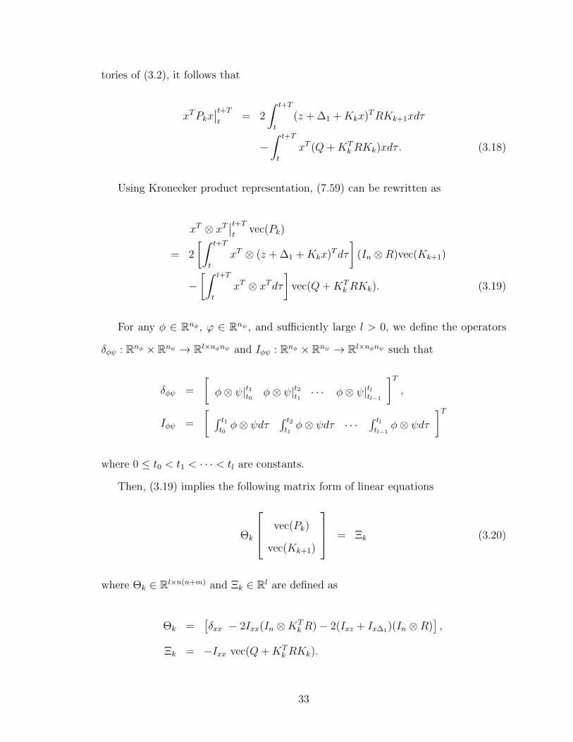
Using Kronecker product representation, (7.59) can be rewritten as
xT ⊗ xT∣∣t+Tt
vec(Pk)
= 2
[∫ t+T
t
xT ⊗ (z + ∆1 +Kkx)Tdτ
](In ⊗R)vec(Kk+1)
−[∫ t+T
t
xT ⊗ xTdτ]
vec(Q+KTk RKk). (3.19)
For any φ ∈ Rnφ , ϕ ∈ Rnψ , and sufficiently large l > 0, we define the operators
δφψ : Rnφ × Rnψ → Rl×nφnψ and Iφψ : Rnφ × Rnψ → Rl×nφnψ such that
δφψ =
[φ⊗ ψ|t1t0 φ⊗ ψ|t2t1 · · · φ⊗ ψ|tltl−1
]T,
Iφψ =
[ ∫ t1t0φ⊗ ψdτ
∫ t2t1φ⊗ ψdτ · · ·
∫ tltl−1
φ⊗ ψdτ]T
where 0 ≤ t0 < t1 < · · · < tl are constants.
Then, (3.19) implies the following matrix form of linear equations
Θk
vec(Pk)
vec(Kk+1)
= Ξk (3.20)
where Θk ∈ Rl×n(n+m) and Ξk ∈ Rl are defined as
Θk =[δxx − 2Ixx(In ⊗KT
k R)− 2(Ixz + Ix∆1)(In ⊗R)],
Ξk = −Ixx vec(Q+KTk RKk).
33
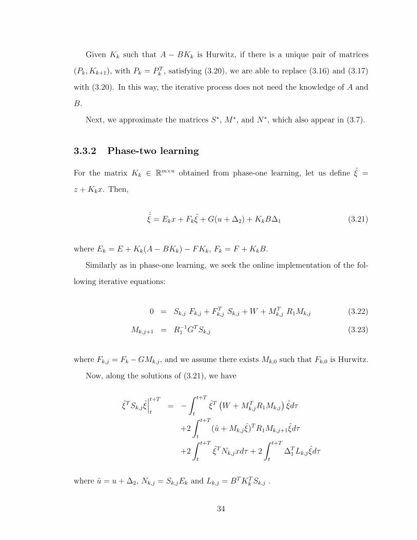
Given Kk such that A − BKk is Hurwitz, if there is a unique pair of matrices
(Pk, Kk+1), with Pk = P Tk , satisfying (3.20), we are able to replace (3.16) and (3.17)
with (3.20). In this way, the iterative process does not need the knowledge of A and
B.
Next, we approximate the matrices S∗, M∗, and N∗, which also appear in (3.7).
3.3.2 Phase-two learning
For the matrix Kk ∈ Rm×n obtained from phase-one learning, let us define ξ =
z +Kkx. Then,
˙ξ = Ekx+ Fkξ +G(u+ ∆2) +KkB∆1 (3.21)
where Ek = E +Kk(A−BKk)− FKk, Fk = F +KkB.
Similarly as in phase-one learning, we seek the online implementation of the fol-
lowing iterative equations:
0 = Sk,j Fk,j + F Tk,j Sk,j +W +MT
k,j R1Mk,j (3.22)
Mk,j+1 = R−11 GTSk,j (3.23)
where Fk,j = Fk −GMk,j, and we assume there exists Mk,0 such that Fk,0 is Hurwitz.
Now, along the solutions of (3.21), we have
ξTSk,j ξ∣∣∣t+T
t= −
∫ t+T
t
ξT(W +MT
k,jR1Mk,j
)ξdτ
+2
∫ t+T
t
(u+Mk,j ξ)TR1Mk,j+1ξdτ
+2
∫ t+T
t
ξTNk,jxdτ + 2
∫ t+T
t
∆T1Lk,j ξdτ
where u = u+ ∆2, Nk,j = Sk,jEk and Lk,j = BTKTk Sk,j .
34
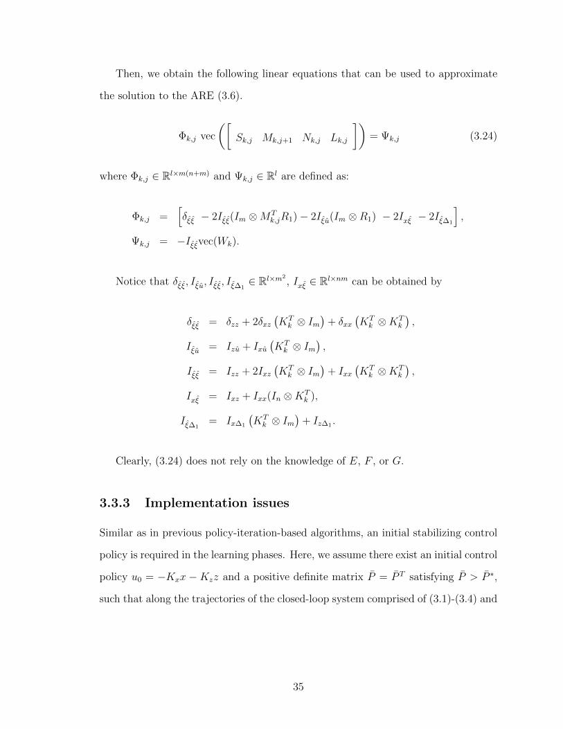
Then, we obtain the following linear equations that can be used to approximate
the solution to the ARE (3.6).
Φk,j vec
([Sk,j Mk,j+1 Nk,j Lk,j
])= Ψk,j (3.24)
where Φk,j ∈ Rl×m(n+m) and Ψk,j ∈ Rl are defined as:
Φk,j =[δξξ − 2Iξξ(Im ⊗MT
k,jR1)− 2Iξu(Im ⊗R1) − 2Ixξ − 2Iξ∆1
],
Ψk,j = −Iξξvec(Wk).
Notice that δξξ, Iξu, Iξξ, Iξ∆1∈ Rl×m2
, Ixξ ∈ Rl×nm can be obtained by
δξξ = δzz + 2δxz(KTk ⊗ Im
)+ δxx
(KTk ⊗KT
k
),
Iξu = Izu + Ixu(KTk ⊗ Im
),
Iξξ = Izz + 2Ixz(KTk ⊗ Im
)+ Ixx
(KTk ⊗KT
k
),
Ixξ = Ixz + Ixx(In ⊗KTk ),
Iξ∆1= Ix∆1
(KTk ⊗ Im
)+ Iz∆1 .
Clearly, (3.24) does not rely on the knowledge of E, F , or G.
3.3.3 Implementation issues
Similar as in previous policy-iteration-based algorithms, an initial stabilizing control
policy is required in the learning phases. Here, we assume there exist an initial control
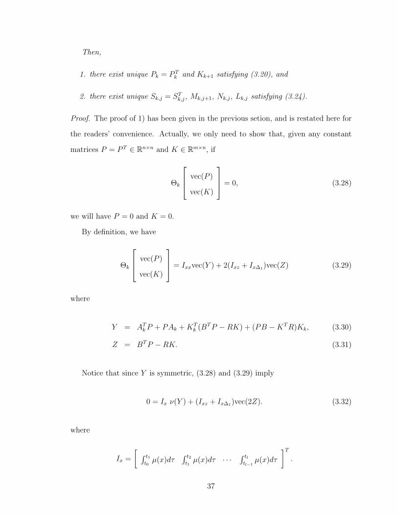
policy u0 = −Kxx −Kzz and a positive definite matrix P = P T satisfying P > P ∗,
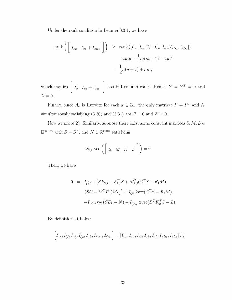
such that along the trajectories of the closed-loop system comprised of (3.1)-(3.4) and
35
u0, we have
d
dt
[XT PX + U(w)
]≤ −ε|X|2 (3.25)
where ε > 0 is a constant.
Notice that this initial stabilizing control policy u0 can be obtained using the idea
of gain assignment [83]. In addition, to satisfy the rank condition in Lemma 3.3.1
below, additional exploration noise may need to be added into the control signal.
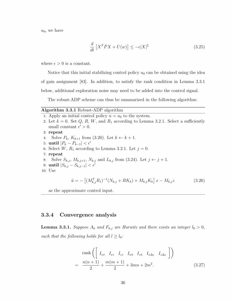
The robust-ADP scheme can thus be summarized in the following algorithm:
Algorithm 3.3.1 Robust-ADP algorithm
1: Apply an initial control policy u = u0 to the system.2: Let k = 0. Set Q, R, W , and R1 according to Lemma 3.2.1. Select a sufficiently
small constant ε′ > 0.3: repeat4: Solve Pk, Kk+1 from (3.20). Let k ← k + 1.5: until |Pk − Pk−1| < ε′
6: Select W , R1 according to Lemma 3.2.1. Let j = 0.7: repeat8: Solve Sk,j, Mk,j+1, Nk,j and Lk,j from (3.24). Let j ← j + 1.9: until |Sk,j − Sk,j−1| < ε′
10: Use
u = −[(MT
k,jR1)−1(Nk,j +RKk) +Mk,jKk
]x−Mk,jz (3.26)
as the approximate control input.
3.3.4 Convergence analysis
Lemma 3.3.1. Suppose Ak and Fk,j are Hurwitz and there exists an integer l0 > 0,
such that the following holds for all l ≥ l0:
rank
([Ixx Ixz Izz Ixu Izu Ix∆1 Iz∆1
])
=n(n+ 1)
2+m(m+ 1)
2+ 3mn+ 2m2. (3.27)
36
Then,
1. there exist unique Pk = P Tk and Kk+1 satisfying (3.20), and
2. there exist unique Sk,j = STk,j, Mk,j+1, Nk,j, Lk,j satisfying (3.24).
Proof. The proof of 1) has been given in the previous setion, and is restated here for
the readers’ convenience. Actually, we only need to show that, given any constant
matrices P = P T ∈ Rn×n and K ∈ Rm×n, if
Θk
vec(P )
vec(K)
= 0, (3.28)
we will have P = 0 and K = 0.
By definition, we have
Θk
vec(P )
vec(K)
= Ixxvec(Y ) + 2(Ixz + Ix∆1)vec(Z) (3.29)
where
Y = ATkP + PAk +KTk (BTP −RK) + (PB −KTR)Kk, (3.30)
Z = BTP −RK. (3.31)
Notice that since Y is symmetric, (3.28) and (3.29) imply
0 = Ix ν(Y ) + (Ixz + Ix∆1)vec(2Z). (3.32)
where
Ix =
[ ∫ t1t0µ(x)dτ
∫ t2t1µ(x)dτ · · ·
∫ tltl−1
µ(x)dτ
]T.
37
Under the rank condition in Lemma 3.3.1, we have
rank
([Ixx Ixz + Ix∆1
])≥ rank ([Ixx, Ixz, Izz, Ixu, Izu, Ix∆1 , Iz∆1 ])
−2mn− 1
2m(m+ 1)− 2m2
=1
2n(n+ 1) +mn,
which implies
[Ix Ixz + Ix∆1
]has full column rank. Hence, Y = Y T = 0 and
Z = 0.
Finally, since Ak is Hurwitz for each k ∈ Z+, the only matrices P = P T and K
simultaneously satisfying (3.30) and (3.31) are P = 0 and K = 0.
Now we prove 2). Similarly, suppose there exist some constant matrices S,M,L ∈
Rm×m with S = ST , and N ∈ Rm×n satisfying
Φk,j vec
([S M N L
])= 0.
Then, we have
0 = Iξξvec[SFk,j + F T
k,jS +MTk,j(G
TS −R1M)
(SG−MTR1)Mk,j
]+ Iξu 2vec(GTS −R1M)
+Ixξ 2vec(SEk −N) + Iξ∆12vec(BTKT
k S − L)
By definition, it holds:
[Ixx, Iξξ, Ixξ, Iξu, Ixu, Ix∆1 , Iξ∆1
]= [Ixx, Ixz, Izz, Ixu, Izu, Ix∆1 , Iz∆1 ]Tn
38
where Tn is a nonsingular matrix. Therefore,
1
2m(m+ 1) + 2m2 +mn
≥ rank
([Iξξ Iξu Ixξ Iξ∆1
])
≥ rank([Ixx, Iξξ, Ixξ, Iξu, Ixu, Ix∆1 , Iξ∆1
])− 1
2n(n+ 1)− 2mn
= rank ([Ixx, Ixz, Izz, Ixu, Izu, Ix∆1 , Iz∆1 ])− 1
2n(n+ 1)− 2mn
=1
2m(m+ 1) + 2m2 +mn.
Following the same reasoning from (3.29) to (3.32), we obtain
0 = SFk,j + F Tk,jS +MT
k,j(GTS −R1M) + (SG−MTR1)Mk,j (3.33)
0 = GTS −R1M, (3.34)
0 = SE −N, (3.35)
0 = BKkS − L (3.36)
where [S,E,M,L] = 0 is the only possible solution.
3.4 Application to synchronous generators
The power system considered in this chapter is an interconnection of two synchronous
generators described by [97]:
∆δi = ∆ωi, (3.37)
∆ωi = − D
2Hi
∆ω +ω0
2Hi
(∆Pmi + ∆Pei) , (3.38)
∆Pmi =1
Ti(−∆Pmi − ki∆ωi + ui) , i = 1, 2 (3.39)
39

where, for the i-th generator, ∆δi, ∆ωi, ∆Pmi, and ∆Pei are the deviations of rotor
angle, relative rotor speed, mechanical input power, and active power, respectively.
The control signal ui represents deviation of the valve opening. Hi, Di, ω0, ki, and
Ti are constant system parameters.
The active power ∆Pei is defined as
∆Pe1 = −E1E2
X[sin(δ1 − δ2)− sin(δ10 − δ20)] (3.40)
and ∆Pe2 = −∆Pe1, where δ10 and δ20 are the steady state angles of the first and
second generators. The second synchronous generator is treated as the dynamic
uncertainty, and it has a fixed controller u2 = −a1∆δ2 − a2∆ω2 − a3∆Pm2, with a1,
a2, and a3 its feedback gains.
Our goal is to design a robust optimal control policy u1 for the interconnected
power system. For simulation purpose, the parameters are specified as follows: D1 =
1, H1 = 3, ω0 = 314.159 rad/s, T1 = 5s, δ10 = 2 rad, D2 = 1, T2 = 5, X = 15,
k2 = 0, H2 = 3, a1 = 0.2236, a2 = −0.2487, a3 = −7.8992. Weighting matrices
are Q = block diag(5, 0.0001), R = 1, W = 0.01, and R1 = 100. The exploration
noise we employed for this simulation is the sum of sinusoidal functions with different
frequencies.
In the simulation, two generators were operated on their steady states from t = 0s
to t = 1s. An impulse disturbance on the load was simulated at t = 1s, and the overall
system started to oscillated. The RADP algorithm was applied to the first generator
from t = 2s to t = 3s. Convergence is attained after six iterations of phase-one
learning followed by ten iterations of phase-two learning, when the stopping criterions
|Pk − Pk−1| ≤ 10−6 and |Sk,j − Sk,j−1| ≤ 10−6 are both satisfied. The linear control
policy formulated after the RADP algorithm is as follows:
u1 = −256.9324∆δ1 − 44.4652∆ω1 − 153.1976∆Pm1.
40
0 1 2 3 4 5 6 7 8 9 100
20
40
60
80
100
120
time (sec)
Rot
or A
ngle
(de
gree
)
Generator 1
0 1 2 3 4 5 6 7 8 9 1060
65
70
75
80
time (sec)
Rot
or A
ngle
(de
gree
)
Generator 2
Robust ADPUnlearned
Robust ADPUnlearned
Oscillation started
Oscillation started
Controller updated
Controller updated
Figure 3.1: Trajectories of the rotor angle.
0 1 2 3 4 5 6 7 8 9 1049.8
49.9
50
50.1
50.2
time (sec)
Fre
quen
cy (
Hz)
Generator 1
0 1 2 3 4 5 6 7 8 9 1049.8
49.9
50
50.1
50.2
time (sec)
Fre
quen
cy (
Hz)
Generator 2
Robust ADPUnlearned
Robust ADPUnlearned
Oscillation started
Oscillation started
Controller updated
Controller updated
Figure 3.2: Trajectories of the angular velocity.
41
The ideal robust optimal control policy is given for comparison as follows
u∗1 = −259.9324∆δ1 − 44.1761∆ω1 − 153.1983∆Pm1.
Trajectories of the output variables and convergence of the feedback gain matrices
are shown in Figures 3.1-3.2.
The new control policy for Generator 1 is applied from t = 3s to the end of
the simulation. It can be seen that oscillation has been significantly reduced after
RADP-based online learning.
3.5 Conclusions
In this chapter, we have proposed a framework of RADP to compute globally asymp-
totically stabilizing control policies with suboptimality and robustness properties in
the presence of dynamic uncertainties. A learning algorithm is provided for the on-
line computation of partial-state feedback control laws. The novel control scheme
is developed by integration of ADP, and some tools developed within the nonlinear
control community. Different from previous ADP schemes in the past literature, the
RADP framework can handle systems with dynamic uncertainties of which the state
variables and the system order are not precisely known. As an illustrative example,
the proposed algorithm has been applied to the robust optimal control for a two-
machine power system. In Chapter 4, the results developed here will be extended to
study multi-machine power systems.
42
Chapter 4
RADP for large-scale systems
The development of intelligent online learning controller gains remarkable popularity
in the operation of large-scale complex systems, such as power systems. In recent
years, considerable attention has been paid to the stabilization of large-scale complex
systems [78], [116], [135], [145], [175], as well as the related consensus and synchro-
nization problems [24], [105], [146], [200]. Examples of large-scale systems arise from
ecosystems, transportation networks, and power systems, to name only a few, [49],
[104], [110], [132], [180], [206]. Often, in real-world applications, precise mathemati-
cal models are hard to build and the model mismatches, caused by parametric and
dynamic uncertainties, are thus unavoidable. This, together with the exchange of
only local system information, makes the design problem extremely challenging in
the context of complex networks.
In this chapter, we intend to extend the RADP theories in Chapters 2 and 3 for
decentralized optimal control of multimachine power systems, and a more generalized
a class of large-scale uncertain systems. The controller design for each subsystem
only needs to utilize local state variables without knowing the system dynamics. By
integrating a simple version of the cyclic-small-gain theorem [109], asymptotic stabil-
ity can be achieved by assigning appropriate weighting matrices for each subsystem.
43
As a by-product, certain suboptimality properties can be obtained.
This chapter is organized as follows. Section 4.1 studies the global and robust
optimal stabilization of a class of large-scale uncertain systems. Section 4.2 develops
the robust ADP scheme for large-scale systems. Section 4.3 presents a novel solution
to decentralized stabilization based on the proposed methodology. It is our belief that
the proposed design methodology will find wide applications in large-scale systems.
Finally, Section 4.4 gives some brief concluding remarks.
4.1 Stability and optimality for large-scale systems
In this section, we first describe the class of large-scale uncertain systems to be stud-
ied. Then, we present our novel decentralized optimal controller design scheme. It will
also be shown that the closed-loop interconnected system enjoys some suboptimality
properties.
4.1.1 Description of large-scale systems
Consider the complex large-scale system of which the i-subsystem (1 ≤ i ≤ N) is
described by
xi = Aixi +Bi [ui + Ψi(y)] , yi = Cixi, 1 ≤ i ≤ N (4.1)
where xi ∈ Rni , yi ∈ Rqi , and ui ∈ Rmi are the state, the output and the control
input for the i-th subsystem; y =[yT1 , y
T2 , · · · , yTN
]T; Ai ∈ Rni×ni , Bi ∈ Rni×mi
are unknown system matrices. Ψi(·) : Rq → Rmi are unknown interconnections
satisfying |Ψi(y)| ≤ di|y| for all y ∈ Rq, with di > 0,∑N
i=1 ni = n,∑N
i=1 qi = q, and∑N
i=1 mi = m. It is also assumed that (Ai, Bi) is a stabilizable pair, that is, there
exists a constant matrix Ki such that Ai −BiKi is a stable matrix.
44
Notice that the decoupled system can be written in a compact form:
x = ADx+BDu (4.2)
where x =[xT1 , x
T2 , · · · , xTN
]T ∈ Rn, u =[uT1 , u
T2 , · · · , uTN
]T ∈ Rm, AD =block
diag(A1, A2, · · · , AN) ∈ Rn×n, BD =block diag(B1, B2,· · · ,BN) ∈ Rn×m.
For system (4.2), we define the following quadratic cost
JD =
∞∫
0
(xTQDx+ uTRDu
)dτ (4.3)
where QD =block diag(Q1,Q2,· · · ,QN) ∈ Rn×n, RD =block diag(R1,R2,· · · , RN) ∈
Rm×m, Qi ∈ Rni×ni , and Ri ∈ Rmi×mi , with Qi = QTi ≥ 0, Ri = RT
i > 0, and
(Ai, Q1/2i ) observable, for all 1 ≤ i ≤ N .
By linear optimal control theory [99], a minimum cost JD in (4.3) can be obtained
by employing the following decentralized control policy
uD = −KDx (4.4)
where KD = block diag(K1, K2, · · · , KN) is given by
KD = R−1D BT
DPD (4.5)
and PD = block diag(P1, P2, · · · , PN) is the unique symmetric positive definite solu-
tion of the algebraic Riccati equation
ATDPD + PDAD − PDBDR−1D BT
DPD +QD = 0. (4.6)
45
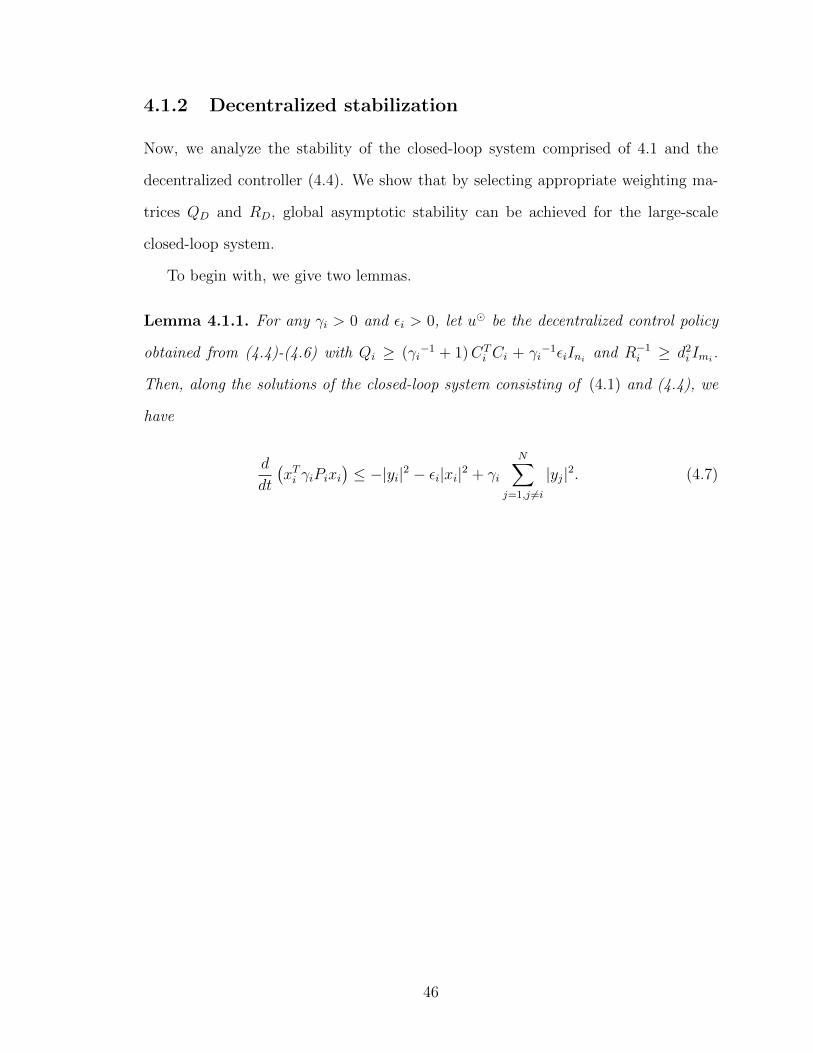
4.1.2 Decentralized stabilization
Now, we analyze the stability of the closed-loop system comprised of 4.1 and the
decentralized controller (4.4). We show that by selecting appropriate weighting ma-
trices QD and RD, global asymptotic stability can be achieved for the large-scale
closed-loop system.
To begin with, we give two lemmas.
Lemma 4.1.1. For any γi > 0 and εi > 0, let u be the decentralized control policy
obtained from (4.4)-(4.6) with Qi ≥ (γi−1 + 1)CT
i Ci + γi−1εiIni and R−1
i ≥ d2i Imi.
Then, along the solutions of the closed-loop system consisting of (4.1) and (4.4), we
have
d
dt
(xTi γiPixi
)≤ −|yi|2 − εi|xi|2 + γi
N∑
j=1,j 6=i
|yj|2. (4.7)
46
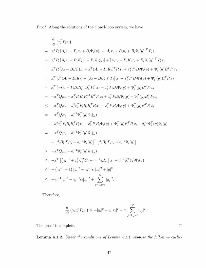
Proof. Along the solutions of the closed-loop system, we have
d
dt
(xTi Pixi
)
= xTi Pi [Aixi +Biui +BiΨi(y)] + [Aixi +Biui +BiΨi(y)]T Pixi
= xTi Pi [Aixi −BiKixi +BiΨi(y)] + [Aixi −BiKixi +BiΨi(y)]T Pixi
= xTi Pi(Ai −BiKi)xi + xTi (Ai −BiKi)TPixi + xTi PiBiΨi(y) + ΨT
i (y)BTi Pixi
= xTi[Pi(Ai −BiKi) + (Ai −BiKi)
TPi]xi + xTi PiBiΨi(y) + ΨT
i (y)BTi Pixi
= xTi[−Qi − PiBiR
−1i BT
i Pi]xi + xTi PiBiΨi(y) + ΨT
i (y)BTi Pixi
= −xTi Qixi − xTi PiBiR−1i BT
i Pixi + xTi PiBiΨi(y) + ΨTi (y)BT
i Pixi
≤ −xTi Qixi − d2ix
Ti PiBiB
Ti Pixi + xTi PiBiΨi(y) + ΨT
i (y)BTi Pixi
= −xTi Qixi + d−2i ΨT
i (y)Ψi(y)
−d2ix
Ti PiBiB
Ti Pixi + xTi PiBiΨi(y) + ΨT
i (y)BTi Pixi − d−2
i ΨTi (y)Ψi(y)
= −xTi Qixi + d−2i ΨT
i (y)Ψi(y)
−[diB
Ti Pixi − d−1
i Ψi(y)]T [
diBTi Pixi − d−1
i Ψi(y)]
≤ −xTi Qixi + d−2i ΨT
i (y)Ψi(y)
≤ −xTi[(γi−1 + 1
)CTi Ci + γi
−1εiIni]xi + d−2
i ΨTi (y)Ψi(y)
≤ −(γi−1 + 1
)|yi|2 − γi−1εi|xi|2 + |y|2
≤ −γi−1|yi|2 − γi−1εi|xi|2 +N∑
j=1,j 6=i
|yj|2.
Therefore,
d
dt
(γix
Ti Pixi
)≤ −|yi|2 − εi|xi|2 + γi
N∑
j=1,j 6=i
|yj|2.
The proof is complete.
Lemma 4.1.2. Under the conditions of Lemma 4.1.1, suppose the following cyclic-
47
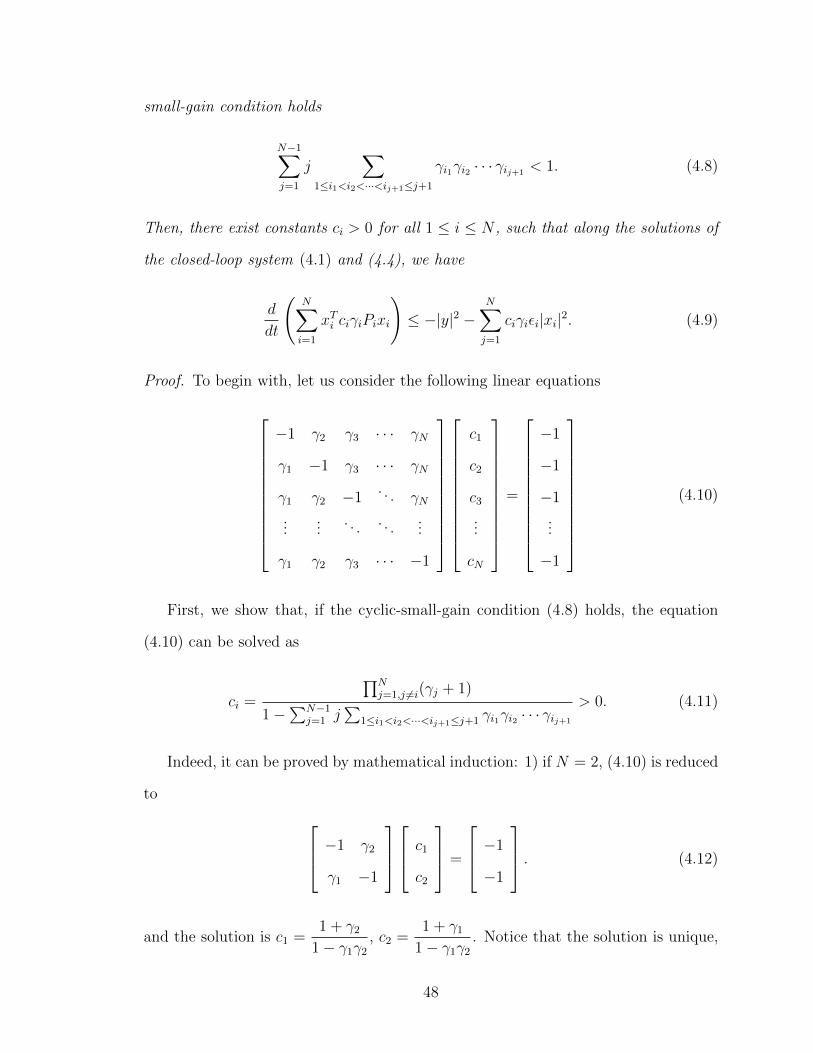
small-gain condition holds
N−1∑
j=1
j∑
1≤i1<i2<···<ij+1≤j+1
γi1γi2 · · · γij+1< 1. (4.8)
Then, there exist constants ci > 0 for all 1 ≤ i ≤ N , such that along the solutions of
the closed-loop system (4.1) and (4.4), we have
d
dt
(N∑
i=1
xTi ciγiPixi
)≤ −|y|2 −
N∑
j=1
ciγiεi|xi|2. (4.9)
Proof. To begin with, let us consider the following linear equations
−1 γ2 γ3 · · · γN
γ1 −1 γ3 · · · γN
γ1 γ2 −1. . . γN
......
. . . . . ....
γ1 γ2 γ3 · · · −1
c1
c2
c3
...
cN
=
−1
−1
−1
...
−1
(4.10)
First, we show that, if the cyclic-small-gain condition (4.8) holds, the equation
(4.10) can be solved as
ci =
∏Nj=1,j 6=i(γj + 1)
1−∑N−1j=1 j
∑1≤i1<i2<···<ij+1≤j+1 γi1γi2 · · · γij+1
> 0. (4.11)
Indeed, it can be proved by mathematical induction: 1) if N = 2, (4.10) is reduced
to
−1 γ2
γ1 −1
c1
c2
=
−1
−1
. (4.12)
and the solution is c1 =1 + γ2
1− γ1γ2
, c2 =1 + γ1
1− γ1γ2
. Notice that the solution is unique,
48

because the cyclic-small-gain condition (4.8) guarantees that the determinant of the
coefficient matrix is non-zero.
2) Suppose (4.11) is the solution of (4.10) with N = N ′ − 1, we show it is also valid
for N = N ′. Then, from the first row of (4.10), we have
−N ′−1∏
j=1,j 6=i
(γj + 1) +N ′−1∑
i=2
N ′−1∏
j=1,j 6=i
(γj + 1)γi
=N ′−2∑
j=1
j∑
1≤i1<i2<···<ij+1≤j+1
γi1γi2 · · · γij+1− 1 (4.13)
Now,
−N ′∏
j=1,j 6=i
(γj + 1) +N ′∑
i=2
N ′∏
j=1,j 6=i
(γj + 1)γi
= −N ′−1∏
j=1,j 6=i
(γj + 1)(γN ′ + 1) +N ′−1∑
i=2
N ′−1∏
j=1,j 6=i
(γj + 1)(γN ′ + 1)γi +N ′−1∏
j=1
(γj + 1)γN ′
=
[−
N ′−1∏
j=1,j 6=i
(γj + 1) +N ′−1∑
i=2
N ′−1∏
j=1,j 6=i
(γj + 1)γi
](γN ′ + 1) +
N ′−1∏
j=1
(γj + 1)γN ′
=
N ′−2∑
j=1
j∑
1≤i1<i2<···<ij+1≤j+1
γi1γi2 · · · γij+1− 1
(γN ′ + 1) +
N ′−1∏
j=1
(γj + 1)γN ′
=N ′−1∑
j=1
j∑
2≤i1<i2<···<ij+1≤j+1
γi1γi2 · · · γij+1+
N ′−2∑
j=1
j∑
1≤i1<i2<···<ij+1≤j+1
γi1γi2 · · · γij+1
+N ′−1∏
j=1
(γj + 1)γN ′ − γN ′ − 1
=N ′−1∑
j=1
j∑
1≤i1<i2<···<ij+1≤j+1
γi1γi2 · · · γij+1− 1.
This implies, with N = N ′, the first row of (4.10) is valid with the solution (4.11).
Same derivations can be applied to the rest rows.
49
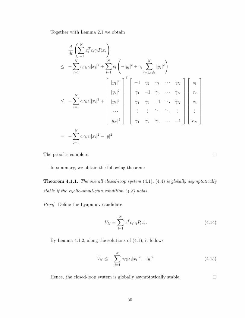
Together with Lemma 2.1 we obtain
d
dt
(N∑
i=1
xTi ciγiPixi
)
≤ −N∑
i=1
ciγiεi|xi|2 +N∑
i=1
ci
(−|yi|2 + γi
N∑
j=1,j 6=i
|yj|2)
≤ −N∑
i=1
ciγiεi|xi|2 +
|y1|2
|y2|2
|y3|2
· · ·
|yN |2
T
−1 γ2 γ3 · · · γN
γ1 −1 γ3 · · · γN
γ1 γ2 −1. . . γN
......
. . . . . ....
γ1 γ2 γ3 · · · −1
c1
c2
c3
...
cN
= −N∑
j=1
ciγiεi|xi|2 − |y|2.
The proof is complete.
In summary, we obtain the following theorem:
Theorem 4.1.1. The overall closed-loop system (4.1), (4.4) is globally asymptotically
stable if the cyclic-small-gain condition (4.8) holds.
Proof. Define the Lyapunov candidate
VN =N∑
i=1
xTi ciγiPixi. (4.14)
By Lemma 4.1.2, along the solutions of (4.1), it follows
VN ≤ −N∑
j=1
ciγiεi|xi|2 − |y|2. (4.15)
Hence, the closed-loop system is globally asymptotically stable.
50
Remark 4.1.1. It is of interest to note that a more generalized cyclic-small-gain
condition based on the notion of input-to-output stability [83], [150] can be found in
[109].
4.1.3 Suboptimality analysis
Suppose Ψi(·) is differentiable at the origin for all 1 ≤ i ≤ N , system (4.1) can be
linearized around the origin as
x = ADx+BDu+ ACx, y = CDx. (4.16)
Notice that under the decentralized control policy (4.4), the cost (4.3) yields a
minimum cost value J⊕D for the coupled system (4.16), which may differ from JD . In
order to study the relationship between J⊕D and JD , define
MD = blockdiag(σ1In1 , σ2In2 , · · · , σNInN ) ∈ Rn×n (4.17)
where σi > 0 with 1 ≤ i ≤ N .
To quantify the suboptimality of the closed-loop system composed of (4.16) and
(4.4), we recall the following concept and theorem from [175]:
Definition 4.1.1 ([175]). The decentralized control law (4.4) is said to be suboptimal
for system (4.1), if there exists a positive number σ such that
J⊕D ≤ σ−1JD . (4.18)
Theorem 4.1.2 ([175]). Suppose there exists a matrix MD as defined in (4.17) such
that the matrix
F (MD) = ATCM−1D PD +M−1
D PDAC + (I −M−1D )(QD +KT
DRDKD) (4.19)
51
satisfy F (MD) ≤ 0. Then, the control uD is suboptimal for (4.16) with degree
σ = min1≤i≤N
σi. (4.20)
The following theorem summarizes the suboptimality of the controller (4.4) under
the cyclic-small-gain condition 4.8.
Theorem 4.1.3. The decentralized controller uD is suboptimal for system (4.1) with
degree
σ = min1≤i≤N
1
ciγimin
1≤i≤N
(ciγi
γiε−1i λM + 1
, 1
)(4.21)
if the condition (4.8) holds.
Proof. Let σ−1i = αciγi with α >
1
min1≤i≤N
(ciγi)and α ≥ 1.
Then, by (4.19) we obtain
d
dt
(xTM−1
D PDx)
= xT(M−1
D PDAD + ADM−1D PD +M−1
D PDAC + ATCM−1D PD
)x
= xT(−M−1
D QD −M−1D KT
DRDKD +M−1D PDAC + ATCM
−1D PD
)x
= xT[F (MD)−QD −KT
DRDKD
]x
52

Therefore, by Lemma 4.1.2, it follows that
xTF (MD)x =d
dt
(xTM−1
D PDx)
+ xT(QD +KT
DRDKD
)x
≤N∑
i=1
xTi[−σ−1
i (Qi − CTi Ci)− α|yi|2 +Qi +KT
i RiKi
]xi
= −N∑
i=1
xTi[σ−1i (Qi − CT
i Ci) + αCTi Ci −Qi −KT
i RiKi
]xi
= −N∑
i=1
xTi[(σ−1i − 1
)(Qi − CT
i Ci)−KTi RiKi
]xi
≤ −N∑
i=1
[(αciγi − 1)
εiγi− λM
]|xi|2
where λM denotes the maximal eigenvalue of KTi RiKi.
Notice that F (MD) ≤ 0, if we set
α = max1≤i≤N
(γiε−1i λM + 1
ciγi, 1
)(4.22)
Therefore, we obtain
σ = min1≤i≤N
1
ciγimin
1≤i≤N
(ciγi
γiε−1i λM + 1
, 1
)(4.23)
The proof is complete by Theorem 4.1.2.
4.2 The RADP design for large-scale systems
Consider the following algebraic Riccati equation
ATi Pi + PiAi +Qi − PiBiR−1i BT
i Pi = 0, 1 ≤ i ≤ N. (4.24)
It has been shown in [89] that, given K(0)i such that Ai − BiK
(0)i is Hurwitz,
53
sequences P (k)i and K(k)
i uniquely determined by
0 = (A(k)i )TP
(k)i + PiA
(k)i +Q
(k)i , (4.25)
K(k+1)i = R−1
i BTi P
(k)i (4.26)
with A(k)i = Ai − BiK
(k)i , and Q
(k)i = Qi + (K
(k)i )TRiK
(k)i , have the properties that
limk→∞
P(k)i = Pi, lim
k→∞K
(k)i = Ki = R−1
i BTi Pi, and A
(k)i is Hurwitz for all k ∈ Z+.
For the i-th subsystem, along the solutions of (4.1), it follows that
xTi P(k)i xi
∣∣∣t+δt
t= 2
∫ t+δt
t
(ui +K(k)i xi)
TRiK(k+1)i xidτ
−∫ t+δt
t
xTi Q(k)i xi dτ (4.27)
where ui = ui + Ψi(y).
For sufficiently large integer li ≥ 0, define δixx ∈ Rli× 12ni(ni+1), I ixx ∈ Rli×n2
i , and
I ixu ∈ Rli×mini as follows
δixx =
[µ(xi)|t1,it0,i µ(xi)|t2,it1,i · · · µ(xi)|tli,itli−1,i
]T,
I ixx =
[ ∫ t1,it0,i
xi ⊗ xidτ∫ t2,it1,i
xi ⊗ xidτ · · ·∫ tli,itli−1,i
xi ⊗ xidτ]T,
I ixu =
[ ∫ t1,it0,i
xi ⊗ uidτ∫ t2,it1,i
xi ⊗ uidτ · · ·∫ tli,itli−1,i
xi ⊗ uidτ]T
where µ(xi) ∈ R 12ni(ni+1) is defined as
µ(xi) =[x2i,1, xi,1xi,2, · · · , xi,1xi,ni , x2
i,2, xi,2xi,3, · · · , xi,ni−1xi,ni , x2i,ni
]T
and 0 ≤ t0,i < t1,i < · · · < tli,i, for i = 1, 2, · · · , N . Also, for any symmetric matrix
54
P ∈ Rni×ni , we define ν(P ) ∈ R 12ni(ni+1) such that
ν(P ) = [p11, 2p12, · · · , 2p1ni , p22, 2p23, · · · , 2pni−1,ni , pni,ni ]T .
Then, (7.59) implies the following matrix form of linear equations
Θ(k)i
ν(P(k)i )
vec(K(k+1)i )
= Ξ
(k)i (4.28)
where the matrices Θ(k)i ∈ Rli× 1
2ni(ni+1)+nimi and Ξ
(k)i ∈ Rli are defined as
Θ(k)i =
[δixx −2I ixx(Ini ⊗ (K
(k)i )TRi)− 2I ixu(Ini ⊗Ri)
],
Ξ(k)i = −I ixx vec(Q
(k)i ).
Clearly, if (4.28) has a unique solution, we are able to replace (4.25) and (4.26)
by (4.28). In this way, the knowledge of both Ai and Bi is no longer needed.
Assumption 4.2.1. rank ([I ixx, Iixu]) =
ni(ni + 1)
2+ nimi.
Theorem 4.2.1. Under Assumption 5.2.1, the matrices P(k)i = (P
(k)i )T and K
(k+1)i
determined by (4.28) satisfy limk→∞
P(k)i = Pi and lim
k→∞K
(k)i = Ki.
Proof. Step 1): First of all, we show that, for each i = 1, 2, · · · , N , and k = 0, 1, · · · ,
equation (4.28) has a unique solution (P(k)i , K
(k+1)i ) with P
(k)i = (P
(k)i )T .
Notice that it amounts to show that the following linear equation
Θ(k)i Xi = 0 (4.29)
has only the trivial solution Xi = 0, for each i = 1, 2, · · · , N , and k = 0, 1, · · ·
To this end, we prove by contradiction: Assume Xi =
Y iv
Ziv
∈ R 1
2ni(ni+1)+mini
55
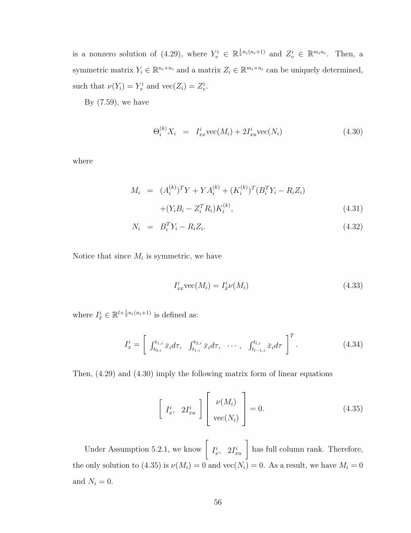
is a nonzero solution of (4.29), where Y iv ∈ R 1
2ni(ni+1) and Zi
v ∈ Rmini . Then, a
symmetric matrix Yi ∈ Rni×ni and a matrix Zi ∈ Rmi×ni can be uniquely determined,
such that ν(Yi) = Y iv and vec(Zi) = Zi
v.
By (7.59), we have
Θ(k)i Xi = I ixxvec(Mi) + 2I ixuvec(Ni) (4.30)
where
Mi = (A(k)i )TY + Y A
(k)i + (K
(k)i )T (BT
i Yi −RiZi)
+(YiBi − ZTi Ri)K
(k)i , (4.31)
Ni = BTi Yi −RiZi. (4.32)
Notice that since Mi is symmetric, we have
I ixxvec(Mi) = I ixν(Mi) (4.33)
where I ix ∈ Rl× 12ni(ni+1) is defined as:
I ix =
[ ∫ t1,it0,i
xidτ,∫ t2,it1,i
xidτ, · · · ,∫ tl,itl−1,i
xidτ
]T. (4.34)
Then, (4.29) and (4.30) imply the following matrix form of linear equations
[I ix, 2I ixu
]
ν(Mi)
vec(Ni)
= 0. (4.35)
Under Assumption 5.2.1, we know
[I ix, 2I ixu
]has full column rank. Therefore,
the only solution to (4.35) is ν(Mi) = 0 and vec(Ni) = 0. As a result, we have Mi = 0
and Ni = 0.
56
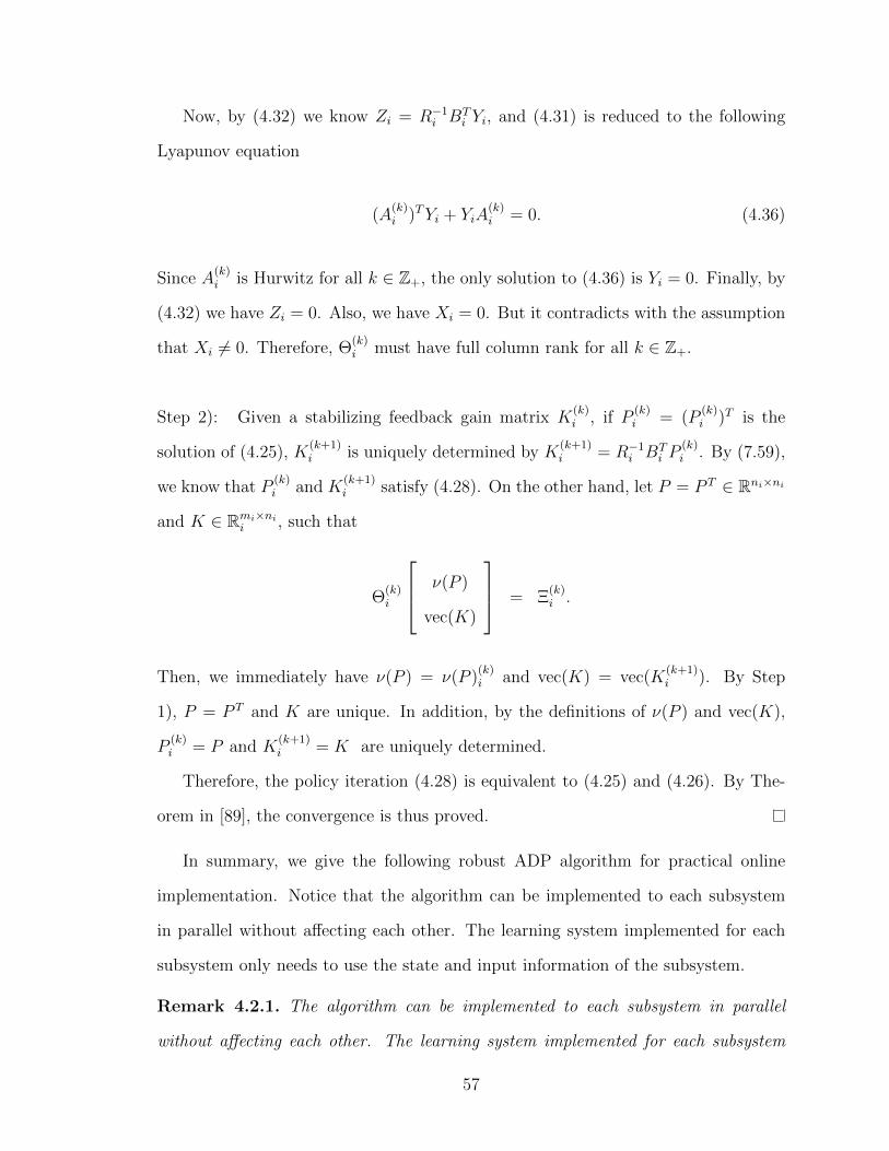
Now, by (4.32) we know Zi = R−1i BT
i Yi, and (4.31) is reduced to the following
Lyapunov equation
(A(k)i )TYi + YiA
(k)i = 0. (4.36)
Since A(k)i is Hurwitz for all k ∈ Z+, the only solution to (4.36) is Yi = 0. Finally, by
(4.32) we have Zi = 0. Also, we have Xi = 0. But it contradicts with the assumption
that Xi 6= 0. Therefore, Θ(k)i must have full column rank for all k ∈ Z+.
Step 2): Given a stabilizing feedback gain matrix K(k)i , if P
(k)i = (P
(k)i )T is the
solution of (4.25), K(k+1)i is uniquely determined by K
(k+1)i = R−1
i BTi P
(k)i . By (7.59),
we know that P(k)i and K
(k+1)i satisfy (4.28). On the other hand, let P = P T ∈ Rni×ni
and K ∈ Rmi×nii , such that
Θ(k)i
ν(P )
vec(K)
= Ξ
(k)i .
Then, we immediately have ν(P ) = ν(P )(k)i and vec(K) = vec(K
(k+1)i ). By Step
1), P = P T and K are unique. In addition, by the definitions of ν(P ) and vec(K),
P(k)i = P and K
(k+1)i = K are uniquely determined.
Therefore, the policy iteration (4.28) is equivalent to (4.25) and (4.26). By The-
orem in [89], the convergence is thus proved.
In summary, we give the following robust ADP algorithm for practical online
implementation. Notice that the algorithm can be implemented to each subsystem
in parallel without affecting each other. The learning system implemented for each
subsystem only needs to use the state and input information of the subsystem.
Remark 4.2.1. The algorithm can be implemented to each subsystem in parallel
without affecting each other. The learning system implemented for each subsystem
57
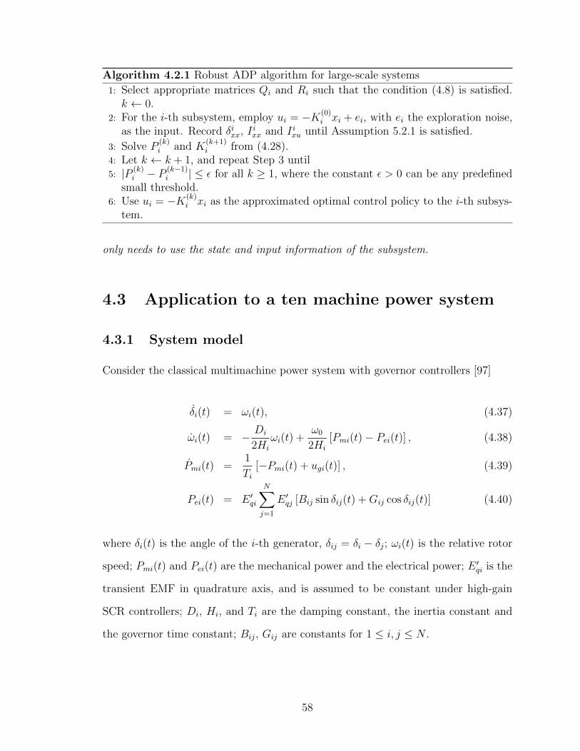
Algorithm 4.2.1 Robust ADP algorithm for large-scale systems
1: Select appropriate matrices Qi and Ri such that the condition (4.8) is satisfied.k ← 0.
2: For the i-th subsystem, employ ui = −K(0)i xi + ei, with ei the exploration noise,
as the input. Record δixx, Iixx and I ixu until Assumption 5.2.1 is satisfied.
3: Solve P(k)i and K
(k+1)i from (4.28).
4: Let k ← k + 1, and repeat Step 3 until5: |P (k)
i − P (k−1)i | ≤ ε for all k ≥ 1, where the constant ε > 0 can be any predefined
small threshold.6: Use ui = −K(k)
i xi as the approximated optimal control policy to the i-th subsys-tem.
only needs to use the state and input information of the subsystem.
4.3 Application to a ten machine power system
4.3.1 System model
Consider the classical multimachine power system with governor controllers [97]
δi(t) = ωi(t), (4.37)
ωi(t) = − Di
2Hi
ωi(t) +ω0
2Hi
[Pmi(t)− Pei(t)] , (4.38)
Pmi(t) =1
Ti[−Pmi(t) + ugi(t)] , (4.39)
Pei(t) = E ′qi
N∑
j=1
E ′qj [Bij sin δij(t) +Gij cos δij(t)] (4.40)
where δi(t) is the angle of the i-th generator, δij = δi − δj; ωi(t) is the relative rotor
speed; Pmi(t) and Pei(t) are the mechanical power and the electrical power; E ′qi is the
transient EMF in quadrature axis, and is assumed to be constant under high-gain
SCR controllers; Di, Hi, and Ti are the damping constant, the inertia constant and
the governor time constant; Bij, Gij are constants for 1 ≤ i, j ≤ N .
58
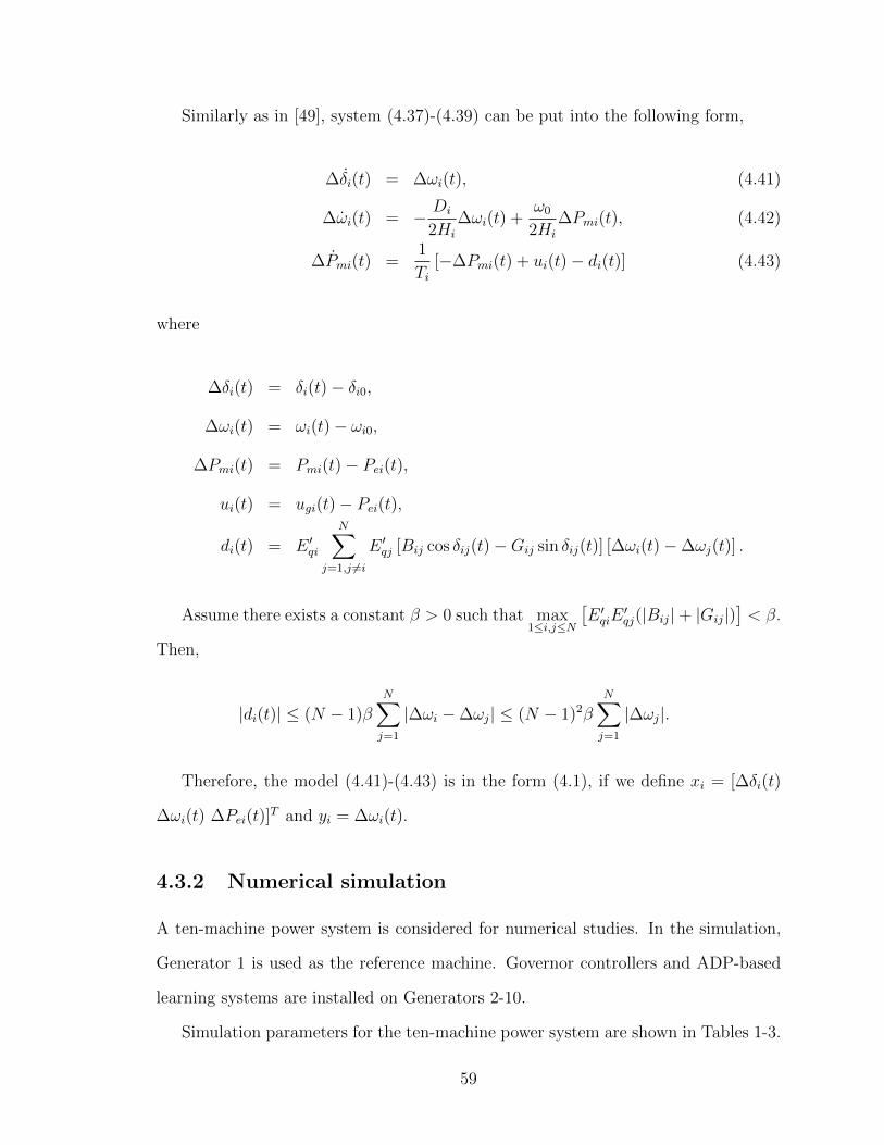
Similarly as in [49], system (4.37)-(4.39) can be put into the following form,
∆δi(t) = ∆ωi(t), (4.41)
∆ωi(t) = − Di
2Hi
∆ωi(t) +ω0
2Hi
∆Pmi(t), (4.42)
∆Pmi(t) =1
Ti[−∆Pmi(t) + ui(t)− di(t)] (4.43)
where
∆δi(t) = δi(t)− δi0,
∆ωi(t) = ωi(t)− ωi0,
∆Pmi(t) = Pmi(t)− Pei(t),
ui(t) = ugi(t)− Pei(t),
di(t) = E ′qi
N∑
j=1,j 6=i
E ′qj [Bij cos δij(t)−Gij sin δij(t)] [∆ωi(t)−∆ωj(t)] .
Assume there exists a constant β > 0 such that max1≤i,j≤N
[E ′qiE
′qj(|Bij|+ |Gij|)
]< β.
Then,
|di(t)| ≤ (N − 1)βN∑
j=1
|∆ωi −∆ωj| ≤ (N − 1)2βN∑
j=1
|∆ωj|.
Therefore, the model (4.41)-(4.43) is in the form (4.1), if we define xi = [∆δi(t)
∆ωi(t) ∆Pei(t)]T and yi = ∆ωi(t).
4.3.2 Numerical simulation
A ten-machine power system is considered for numerical studies. In the simulation,
Generator 1 is used as the reference machine. Governor controllers and ADP-based
learning systems are installed on Generators 2-10.
Simulation parameters for the ten-machine power system are shown in Tables 1-3.
59
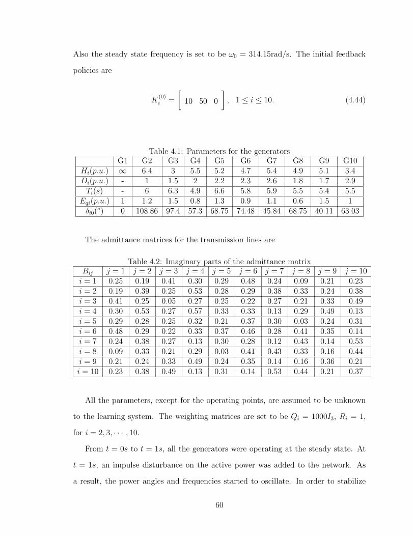
Also the steady state frequency is set to be ω0 = 314.15rad/s. The initial feedback
policies are
K(0)i =
[10 50 0
], 1 ≤ i ≤ 10. (4.44)
Table 4.1: Parameters for the generatorsG1 G2 G3 G4 G5 G6 G7 G8 G9 G10
Hi(p.u.) ∞ 6.4 3 5.5 5.2 4.7 5.4 4.9 5.1 3.4Di(p.u.) - 1 1.5 2 2.2 2.3 2.6 1.8 1.7 2.9Ti(s) - 6 6.3 4.9 6.6 5.8 5.9 5.5 5.4 5.5
Eqi(p.u.) 1 1.2 1.5 0.8 1.3 0.9 1.1 0.6 1.5 1δi0() 0 108.86 97.4 57.3 68.75 74.48 45.84 68.75 40.11 63.03
The admittance matrices for the transmission lines are
Table 4.2: Imaginary parts of the admittance matrixBij j = 1 j = 2 j = 3 j = 4 j = 5 j = 6 j = 7 j = 8 j = 9 j = 10i = 1 0.25 0.19 0.41 0.30 0.29 0.48 0.24 0.09 0.21 0.23i = 2 0.19 0.39 0.25 0.53 0.28 0.29 0.38 0.33 0.24 0.38i = 3 0.41 0.25 0.05 0.27 0.25 0.22 0.27 0.21 0.33 0.49i = 4 0.30 0.53 0.27 0.57 0.33 0.33 0.13 0.29 0.49 0.13i = 5 0.29 0.28 0.25 0.32 0.21 0.37 0.30 0.03 0.24 0.31i = 6 0.48 0.29 0.22 0.33 0.37 0.46 0.28 0.41 0.35 0.14i = 7 0.24 0.38 0.27 0.13 0.30 0.28 0.12 0.43 0.14 0.53i = 8 0.09 0.33 0.21 0.29 0.03 0.41 0.43 0.33 0.16 0.44i = 9 0.21 0.24 0.33 0.49 0.24 0.35 0.14 0.16 0.36 0.21i = 10 0.23 0.38 0.49 0.13 0.31 0.14 0.53 0.44 0.21 0.37
All the parameters, except for the operating points, are assumed to be unknown
to the learning system. The weighting matrices are set to be Qi = 1000I3, Ri = 1,
for i = 2, 3, · · · , 10.
From t = 0s to t = 1s, all the generators were operating at the steady state. At
t = 1s, an impulse disturbance on the active power was added to the network. As
a result, the power angles and frequencies started to oscillate. In order to stabilize
60
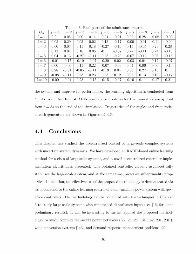
Table 4.3: Real parts of the admittance matrixGij j = 1 j = 2 j = 3 j = 4 j = 5 j = 6 j = 7 j = 8 j = 9 j = 10i = 1 0.21 0.05 0.00 0.14 0.04 -0.01 0.00 0.28 -0.08 -0.00i = 2 0.05 0.29 0.03 0.02 0.13 -0.17 -0.00 -0.01 -0.11 -0.04i = 3 0.00 0.03 0.15 0.18 -0.27 -0.10 0.15 -0.05 0.23 0.28i = 4 0.13 0.01 0.18 0.05 -0.11 -0.07 0.22 -0.11 0.24 -0.15i = 5 0.04 0.13 -0.27 -0.11 0.08 -0.20 -0.07 -0.19 0.03 -0.15i = 6 -0.01 -0.17 -0.10 -0.07 -0.20 0.02 -0.03 0.04 0.12 -0.07i = 7 0.00 -0.00 0.15 0.22 -0.07 -0.03 0.04 0.06 0.06 -0.10i = 8 0.28 -0.01 -0.05 -0.11 -0.19 0.04 0.06 0.27 0.13 0.11i = 9 -0.08 -0.11 0.23 0.23 0.03 0.12 0.06 0.13 0.19 -0.17i = 10 -0.00 -0.04 0.28 -0.15 -0.15 -0.07 -0.10 0.11 -0.17 0.21
the system and improve its performance, the learning algorithm is conducted from
t = 4s to t = 5s. Robust ADP-based control policies for the generators are applied
from t = 5s to the end of the simulation. Trajectories of the angles and frequencies
of each generators are shown in Figures 4.1-4.6.
4.4 Conclusions
This chapter has studied the decentralized control of large-scale complex systems
with uncertain system dynamics. We have developed an RADP-based online learning
method for a class of large-scale systems, and a novel decentralized controller imple-
mentation algorithm is presented. The obtained controller globally asymptotically
stabilizes the large-scale system, and at the same time, preserves suboptimality prop-
erties. In addition, the effectiveness of the proposed methodology is demonstrated via
its application to the online learning control of a tem-machine power system with gov-
ernor controllers. The methodology can be combined with the techniques in Chapter
3 to study large-scale systems with unmatched disturbance input (see [16] for some
preliminary results). It will be interesting to further applied the proposed method-
ology to study complex real-world power networks ([27, 25, 26, 134, 152, 201, 201]),
wind conversion systems [143], and demand response management problems [29].
61
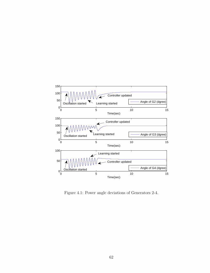
0 5 10 150
50
100
150
Time(sec)
Angle of G2 (dgree)
0 5 10 150
50
100
150
Time(sec)
Angle of G3 (dgree)
0 5 10 150
50
100
Time(sec)
Angle of G4 (dgree)
Oscillation started
Oscillation started
Oscillation started
Learning started
Learning started
Controller updated
Controller updated
Learning started
Controller updated
Figure 4.1: Power angle deviations of Generators 2-4.
62
0 5 10 150
100
200
300
Time(sec)
Angle of G5 (dgree)
0 5 10 150
50
100
150
Time(sec)
Angle of G6 (dgree)
0 5 10 15−50
0
50
100
Time(sec)
Angle of G7 (dgree)
Oscillation started
Oscillation started Learning started
Controller updated
Controller updated
Learning started
Oscillation started Learning started
Controller updated
Figure 4.2: Power angle deviations of Generators 5-7.
0 5 10 150
50
100
150
Time(sec)
Angle of G8 (dgree)
0 5 10 1520
40
60
80
Time(sec)
Angle of G9 (dgree)
0 5 10 1540
60
80
100
Time(sec)
Angle of G10 (dgree)Learning started
Oscillation started
Oscillation started
Oscillation started
Learning started
Controller updated
Learning started
Controller updated
Controller updated
Figure 4.3: Power angle deviations of Generators 8-10.
63
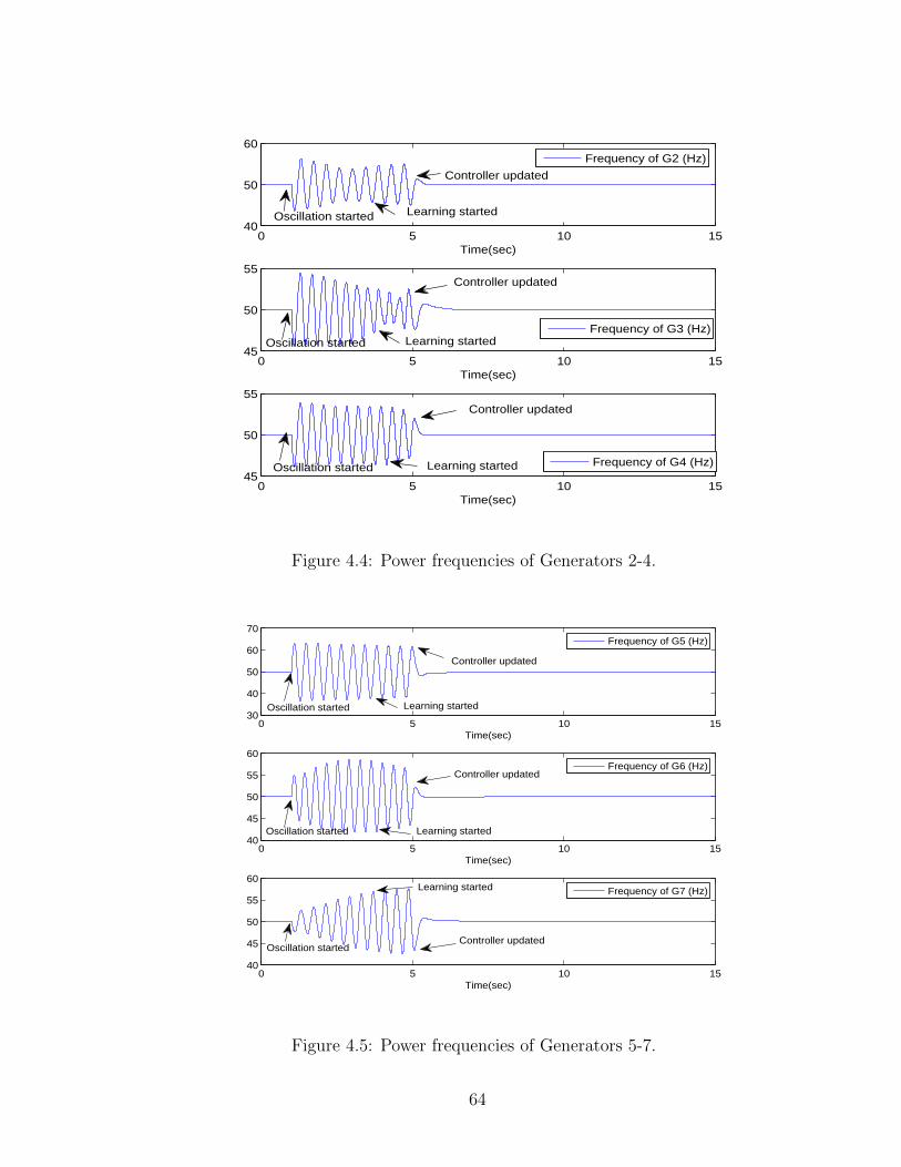
0 5 10 1540
50
60
Time(sec)
Frequency of G2 (Hz)
0 5 10 1545
50
55
Time(sec)
Frequency of G3 (Hz)
0 5 10 1545
50
55
Time(sec)
Frequency of G4 (Hz)Oscillation started
Controller updated
Oscillation started Learning started
Controller updated
Oscillation started Learning started
Controller updated
Learning started
Figure 4.4: Power frequencies of Generators 2-4.
0 5 10 1530
40
50
60
70
Time(sec)
Frequency of G5 (Hz)
0 5 10 1540
45
50
55
60
Time(sec)
Frequency of G6 (Hz)
0 5 10 1540
45
50
55
60
Time(sec)
Frequency of G7 (Hz)
Oscillation started
Oscillation started
Oscillation startedController updated
Controller updated
Controller updated
Learning started
Learning started
Learning started
Figure 4.5: Power frequencies of Generators 5-7.
64
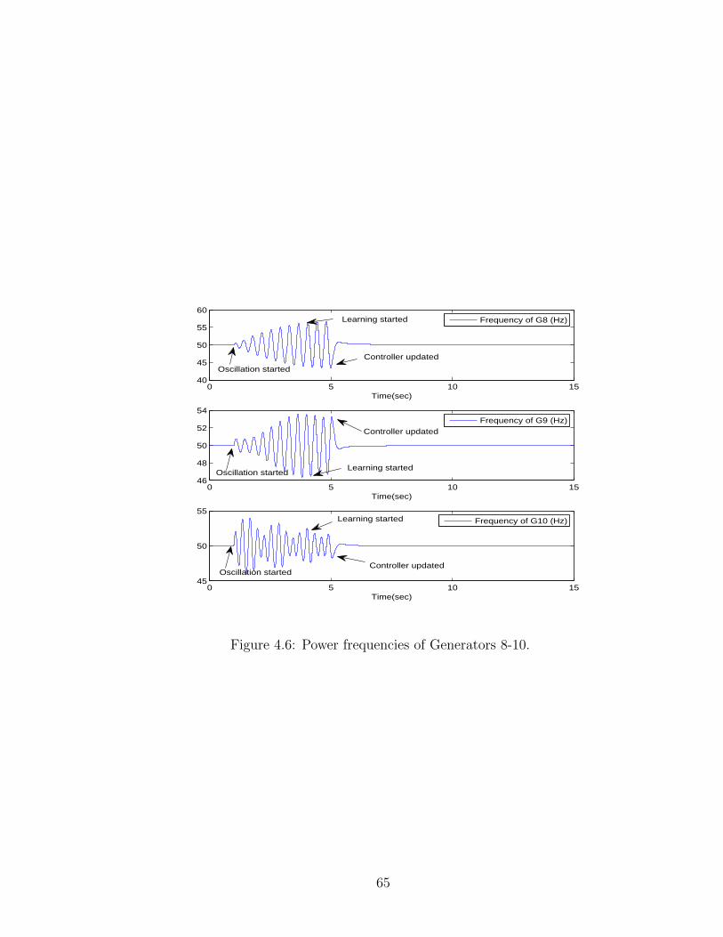
0 5 10 1540
45
50
55
60
Time(sec)
Frequency of G8 (Hz)
0 5 10 1546
48
50
52
54
Time(sec)
Frequency of G9 (Hz)
0 5 10 1545
50
55
Time(sec)
Frequency of G10 (Hz)Learning started
Oscillation started
Controller updated
Learning started
Oscillation startedLearning started
Controller updated
Controller updatedOscillation started
Figure 4.6: Power frequencies of Generators 8-10.
65
Chapter 5
Neural-networks-based RADP for
nonlinear systems
As mentioned in Chapter 3, a common assumption in the past literature of ADP
is that the system order is known and the state variables are either fully available
or reconstructible from the output [101]. This problem, often formulated in the
context of robust control theory, cannot be viewed as a special case of output feedback
control. In addition, the ADP methods developed in the past literature may fail to
guarantee not only optimality, but also the stability of the closed-loop system when
dynamic uncertainty occurs. The RADP framework is developed to bridge the above-
mentioned gap in the past literature of ADP, and it can be viewed as an extension of
ADP to linear and partially linear systems [161], [164] with dynamic uncertainties.
This chapter studies RADP designs for genuinely nonlinear systems in the pres-
ence of dynamic uncertainties. We first decompose the open-loop system into two
parts: The system model (ideal environment) with known system order and fully ac-
cessible state, and the dynamic uncertainty, with unknown system order, dynamics,
and unmeasured states, interacting with the ideal environment. In order to handle
the dynamic interaction between two systems, we resort to the gain assignment idea
66
[83], [129]. More specifically, we need to assign a suitable gain for the system model
with disturbance in the sense of Sontag’s input-to-state stability (ISS) [149], [151].
The backstepping, robust redesign, and small-gain techniques in modern nonlinear
control theory are incorporated into the RADP theory, such that the system mod-
el is made ISS with an arbitrarily small gain. To perform stability analysis for the
interconnected systems, we apply the nonlinear small-gain theorem [83], which has
been proved to be an efficient tool for nonlinear system analysis and synthesis. As a
consequence, the proposed RADP method can be seen as a nonlinear variant of [68].
Moreover, it solves the semi-global stabilization problem [161] in the sense that the
domain of attraction for the closed-loop system can be made as large as possible.
The remainder of the paper is organized as follows. Section 5.1 reviews the on-
line policy iteration technique for affine nonlinear systems. Section 5.2 studies the
methodology of robust optimal design and gives a practical algorithm. Section 5.3
extends the RADP theory to nonlinear systems with unmatched dynamic uncertain-
ties. Two numerical examples, including the controller designs for a jet engine and
for a synchronous power generator, are provided in Section 5.4. Finally, concluding
remarks are given in Section 5.5.
5.1 Problem formulation and preliminarlies
5.1.1 Nonlinear optimal control
Consider the system
x = f(x) + g(x)u (5.1)
where x ∈ Rn is the system state, u ∈ R is the control input, f, g : Rn → Rn are
locally Lipschitz functions. The to-be-minimized cost associated with (5.1) is defined
67

as
J(x0, u) =
∫ ∞
0
[Q(x) + ru2
]dt, x(0) = x0 (5.2)
where Q(·) is a positive definite function, and r > 0 is a constant. In addition,
assume there exists an admissible control policy u = u0(x) in the sense that, under
this policy, the system (5.1) is globally asymptotically stable and the cost (5.2) is
finite. By [99], the control policy that minimizes the cost (5.2) can be solved from
the following Hamilton-Jacobi-Bellman (HJB) equation:
0 = ∇V (x)Tf(x) +Q(x)− 1
4r
[∇V (x)Tg(x)
]2(5.3)
with the boundary condition V (0) = 0. Indeed, if the solution V ∗(x) of (5.3) exists,
the optimal control policy is given by
u∗(x) = − 1
2rg(x)T∇V ∗(x). (5.4)
In general, the analytical solution of (5.3) is difficult to be obtained. However, if
V ∗(x) exists, it can be approximated using the policy iteration technique [136]:
Algorithm 5.1.1 Nonlinear policy iteration algorithm
1: Find an admissible control policy u0(x).2: For any integer i ≥ 0, solve for Vi(x), with Vi(0) = 0, from
0 = ∇Vi(x)T [f(x) + g(x)ui(x)] +Q(x) + rui(x)2. (5.5)
3: Update the control policy by
ui+1(x) = − 1
2rg(x)T∇Vi(x). (5.6)
Convergence of the policy iteration (5.5) and (5.6) is concluded in the following
theorem, the proof of which follows the same lines of reasoning as in the proof of [136,
68

Theorem 4].
Theorem 5.1.1. Consider Vi(x) and ui+1(x) defined in (5.5) and (5.6). Then, for
all i = 0, 1, · · · ,
0 ≤ Vi+1(x) ≤ Vi(x), ∀x ∈ Rn (5.7)
and ui+1(x) is admissible. In addition, if the solution V ∗(x) of (5.3) exists, then
for each fixed x, Vi(x)∞i=0 and ui(x)∞i=0 converge pointwise to V ∗(x) and u∗(x),
respectively.
5.2 Online Learning via RADP
In this section, we develop the RADP methodology for nonlinear systems as follows:
w = ∆w(w, x) (5.8)
x = f(x) + g(x) [u+ ∆(w, x)] (5.9)
where x ∈ Rn is the measured component of the state available for feedback control,
w ∈ Rp is the unmeasurable part of the state with unknown order p, u ∈ R is the
control input, ∆w : Rp × Rn → Rp, ∆ : Rp × Rn → R are unknown locally Lipschitz
functions, f and g are defined the same as in (5.1) but are assumed to be unknown.
Our design objective is to find online the control policy which stabilizes the system
at the origin. Also, in the absence of the dynamic uncertainty (i.e., ∆ = 0 and the
w-subsystem is absent), the control policy becomes the optimal control policy that
minimizes (5.2).
69
5.2.1 Online policy iteration
The iterative technique introduced in Section 5.1 relies on the knowledge of both f(x)
and g(x). To remove this requirement, we develop a novel online policy iteration
technique, which can be viewed as the nonlinear extension of [68].
To begin with, notice that (5.9) can be rewritten as
x = f(x) + g(x)ui(x) + g(x)vi (5.10)
where vi = u+∆−ui. For each i ≥ 0, the time derivative of Vi(x) along the solutions
of (5.10) satisfies
Vi = ∇Vi(x)T [f(x) + g(x)ui(x) + g(x)vi]
= −Q(x)− ru2i (x) +∇Vi(x)Tg(x)vi
= −Q(x)− ru2i (x)− 2rui+1(x)vi. (5.11)
Integrating both sides of (5.11) on any time interval [t, t+ T ], it follows that
Vi(x(t+ T ))− Vi(x(t))
=
∫ t+T
t
[−Q(x)− ru2
i (x)− 2rui+1(x)vi]dτ. (5.12)
Notice that, if an admissible control policy ui(x) is given, the unknown functions
Vi(x) and ui+1(x) can be approximated using (5.12). To be more specific, for any given
compact set Ω ⊂ Rn containing the origin as an interior point, let φj(x)∞j=1 be an
infinite sequence of linearly independent smooth basis functions on Ω, where φj(0) = 0
for all j = 1, 2, · · · . Then, by approximation theory [126], for each i = 0, 1, · · · , the
70
cost function and the control policy can be approximated by:
Vi(x) =
N1∑
j=1
ci,jφj(x), (5.13)
ui+1(x) =
N2∑
j=1
wi,jφj(x). (5.14)
where N1 > 0, N2 > 0 are two sufficiently large integers, and ci,j, wi,j are constant
weights to be determined.
Replacing Vi(x), ui(x), and ui+1(x) in (5.12) with their approximations, we obtain
N1∑
j=1
ci,j [φj(x(tk+1))− φj(x(tk))]
= −∫ tk+1
tk
2r
N2∑
j=1
wi,jφj(x)vidt (5.15)
−∫ tk+1
tk
[Q(x) + ru2
i (x)]dt+ ei,k
where u0 = u0, vi = u + ∆ − ui, and tklk=0 is a strictly increasing sequence with
l > 0 a sufficiently large integer. Then, the weights ci,j and wi,j can be solved in the
sense of least-squares (i.e., by minimizing∑l
k=0 e2i,k).
Now, starting from u0(x), two sequences Vi(x)∞i=0, and ui+1(x)∞i=0 can be gen-
erated via the online policy iteration technique (5.15). Next, we show the convergence
of the sequences to Vi(x) and ui+1(x), respectively.
Assumption 5.2.1. There exist l0 > 0 and δ > 0, such that for all l ≥ l0, we have
1
l
l∑
k=0
θTi,kθi,k ≥ δIN1+N2 (5.16)
71
where
θTi,k =
φ1(x(tk+1))− φ1(x(tk))
φ2(x(tk+1))− φ2(x(tk))
...
φN1(x(tk+1))− φN1(x(tk))
2r∫ tk+1
tkφ1(x)vidt
2r∫ tk+1
tkφ2(x)vidt
...
2r∫ tk+1
tkφN2(x)vidt
∈ RN1+N2 .
Assumption 5.2.2. The closed-loop system composed of (5.8), (5.9), and
u = u0(x) + e (5.17)
is ISS when e, the exploration noise, is considered as the input.
Remark 5.2.1. The reason for imposing Assumption 5.2.2 is twofold. First, like in
many other policy-iteration-based ADP algorithms, an initial admissible control policy
is desired. Inspired by [205], we further assume the initial control policy is stabilizing
in the presence of dynamic uncertainties. Such an assumption is feasible and realistic
by means of the designs in [80], [129]. Second, by adding the exploration noise, we
are able to satisfy Assumption 5.2.1, and at the same time keep the system solutions
bounded.
Under Assumption 5.2.2, we can find a compact set Ω0 which is an invariant set
of the closed-loop system composed of (5.8), (5.9), and u = u0(x). In addition, we
can also let Ω0 contain Ωi∗ as its subset. Then, the compact set for approximation
can be selected as Ω = x : ∃w, s.t. (w, x) ∈ Ω0.
72
Theorem 5.2.1. Under Assumptions 5.2.1 and 5.2.2, for each i ≥ 0 and given ε > 0,
there exist N∗1 > and N∗2 > 0, such that
|N1∑
j=1
ci,jφj(x)− Vi(x)| < ε, (5.18)
|N2∑
j=1
wi,jφj(x)− ui+1(x)| < ε, (5.19)
for all x ∈ Ω., if N1 > N∗1 and N2 > N∗2 .
Proof. To begin with, given ui, let Vi(x) be the solution of the following equation
with Vi(0) = 0.
∇Vi(x)T (f(x) + g(x)ui(x)) +Q(x) + ru2i (x) = 0 (5.20)
and denote ui+1(x) = − 1
2rg(x)T∇Vi(x)T .
Lemma 5.2.1. For each i ≥ 0, we have limN1,N2→∞
Vi(x) = Vi(x), limN1,N2→∞
ui+1(x) =
ui+1(x), ∀x ∈ Ω.
Proof. By definition
Vi(x(tk+1))− Vi(x(tk))
= −∫ tk+1
tk
[Q(x) + ru2i (x) + 2rui+1(x)vi]dt (5.21)
Let ci,j and wi,j be the constant weights such that Vi(x) =∑∞
j=1 ci,jφj(x) and
ui+1(x) =∑∞
j=1 wi,jφj(x). Then, by (5.15) and (5.21), we have ei,k = θTi,kWi + ξi,k,
73
where
Wi =
[ci,1 ci,2 · · · ci,N1
wi,1 wi,2 · · · wi,N2
]T
−[ci,1 ci,2 · · · ci,N1
wi,1 wi,2 · · · wi,N2
]T,
ξi,k =∞∑
j=N1+1
ci,j [φj(x(tk+1))− φj(x(tk))]
+∞∑
j=N2+1
wi,j
∫ tk+1
tk
2rφj(x)vidt.
Since the weights are found using the least-squares method, we have
l∑
k=1
e2i,k ≤
l∑
k=1
ξ2i,k
Also, notice that,
l∑
k=1
W Ti θ
Ti,kθi,kWi =
l∑
k=1
(ei,k − ξi,k)2
Then, under Assumption 5.2.1, it follows that
¯|Wi|2 ≤4|Ξi,l|2lδ
=4
δmax1≤k≤l
ξ2i,k.
Therefore, given any arbitrary ε > 0, we can find N10 > 0 and N20 > 0, such that
when N1 > N10 and N2 > N20, we have
|Vi(x)− Vi(x)|
≤N1∑
j=1
|ci,j − ci,j||φj(x)|+∞∑
j=N1+1
|ci,jφj(x)|
≤ ε
2+ε
2= ε, ∀x ∈ Ω. (5.22)
74
Similarly, |ui+1(x)− ui+1(x)| ≤ ε. The proof is complete.
We now prove Theorem 5.2.1 by induction:
1) If i = 0 we have V0(x) = V0(x), and u1(x) = u1(x). Hence, the convergence can
directly be proved by Lemma A.1.
2) Suppose for some i > 0, we have limN1,N2→∞ Vi−1(x) = Vi−1(x), limN1,N2→∞ ui(x) =
ui(x), ∀x ∈ Ω. By definition, we have
|Vi(x(t))− Vi(x(t))|
= r|∫ ∞
t
[ui(x)2 − ui(x)2
]dt|
+ 2r|∫ ∞
t
ui+1(x) [ui(x)− ui(x)] dt|
+ 2r|∫ ∞
t
[ui+1(x)− ui+1(x)] vidt|, ∀x ∈ Ω.
By the induction assumptions, we know
limN1,N2→∞
∫ ∞
t
[ui(x)2 − ui(x)2
]dt = 0 (5.23)
limN1,N2→∞
∫ ∞
t
ui+1(x) [ui(x)− ui(x)] dt = 0 (5.24)
Also, by Assumption 5.2.1, we conclude
limN1,N2→∞
|ui+1(x)− ui+1(x)| = 0 (5.25)
and
limN1,N2→∞
|Vi(x)− Vi(x)| = 0. (5.26)
75
Finally, since
|Vi(x)− Vi(x)| ≤ |Vi(x)− Vi(x)|+ |Vi(x)− Vi(x)|
and by the induction assumption, we have
limN1,N2→∞
|Vi(x)− Vi(x)| = 0. (5.27)
Similarly, we can show
limN1,N2→∞
|ui+1(x)− ui(x)| = 0. (5.28)
The proof is thus complete.
Corollary 5.2.1. Assume V ∗(x) and u∗(x) exist. Then, under Assumptions 5.2.1
and 5.2.2, for any arbitrary ε > 0, there exist integers i∗ > 0, N∗∗1 > 0 and N∗∗2 > 0,
such that
|N1∑
j=1
ci∗,jφj(x)− V ∗(x)| ≤ ε, (5.29)
|N2∑
j=1
wi∗,jφj(x)− u∗(x)| ≤ ε, (5.30)
for all x ∈ Ω, if N1 > N∗∗1 , and N2 > N∗∗2 .
Proof. By Theorem 6.1.1, there exists i∗ > 0, such that
|Vi∗(x)− V ∗(x)| ≤ ε
2, (5.31)
|ui∗+1(x)− u∗(x)| ≤ ε
2, ∀x ∈ Ω. (5.32)
By Theorem 5.2.1, there exist N∗∗1 > 0 and N∗∗2 > 0, such that for all N1 > N∗∗1
76
and N2 > N∗∗2 ,
|N1∑
j=1
ci∗,jφj(x)− Vi∗(x)| ≤ ε
2, (5.33)
|N2∑
j=1
wi∗,jφj(x)− ui∗+1(x)| ≤ ε
2, ∀x ∈ Ω. (5.34)
The corollary is thus proved by using the triangle inequality.
5.2.2 Robust redesign
In the presence of the dynamic uncertainty, we redesign the approximated optimal
control policy so as to achieve robust stability. The proposed method is an integration
of optimal control theory [99] with the gain assignment technique [83], [129]. To begin
with, let us make the following assumptions.
Assumption 5.2.3. There exists a function α of class K∞, such that for i = 0, 1, · · · ,
α(|x|) ≤ Vi(x), ∀x ∈ Rn. (5.35)
In addition, assume there exists a constant ε > 0 such that Q(x)− ε2|x|2 is a positive
definite function.
Notice that, we can also find a class K∞ function α, such that for i = 0, 1, · · · ,
Vi(x) ≤ α(|x|), ∀x ∈ Rn. (5.36)
Assumption 5.2.4. Consider (5.8). There exist functions λ, λ ∈ K∞, κ1, κ2, κ3 ∈ K,
and positive definite functions W and κ4, such that for all w ∈ Rp and x ∈ Rn, we
77
have
λ(|w|) ≤ W (w) ≤ λ(|w|), (5.37)
|∆(w, x)| ≤ maxκ1(|w|), κ2(|x|), (5.38)
together with the following implication:
W (w) ≥ κ3(|x|)⇒ ∇W (w)∆w(w, x) ≤ −κ4(w). (5.39)
Assumption 6.6.1 implies that the w-system (5.8) is input-to-state stable (ISS)
[149], [151] when x is considered as the input.
Now, consider the following type of control policy
uro(x) =[1 +
r
2ρ2(|x|2)
]ui∗+1(x) (5.40)
where i∗ > 0 is a sufficiently large integer as defined in Corollary 5.2.1, ρ is a smooth,
non-decreasing function, with ρ(s) > 0 for all s ≥ 0. Notice that uro can be viewed
as a robust redesign of the approximated optimal control policy ui∗+1.
As in [80], let us define a class K∞ function γ by
γ(s) =1
2ερ(s2)s, ∀s ≥ 0. (5.41)
In addition, define
ero(x) =r
2ρ2(|x|2) [ui∗+1(x)− ui∗+1(x)]
+ui∗+1(x)− ui∗(x). (5.42)
78
Theorem 5.2.2. Under Assumptions 5.2.3 and 6.6.1, suppose
γ > maxκ2, κ1 λ−1 κ3 α−1 α, (5.43)
and the following implication holds for some constant d > 0:
0 < Vi∗(x) ≤ d⇒ |ero(x)| < γ(|x|). (5.44)
Then, the closed-loop system composed of (5.8), (5.9), and (5.40) is asymptotically
stable at the origin. In addition, there exists σ ∈ K∞, such that Ωi∗ = (w, x) :
max [σ(Vi∗(x)),W (w)] ≤ σ(d) is an estimate of the region of attraction of the closed-
loop system.
Proof. Define
ero(x) =
ero(x), Vi∗(x) ≤ d
0, Vi∗(x) > d(5.45)
and
u(x) = ui∗(x) +r
2ρ2(|x|2)ui∗+1(x) + ero(x). (5.46)
Then, along the solutions of (5.9), by completing the squares, we have
Vi∗ ≤ −Q(x) +1
ρ2(|x|2)(∆ + ero(x))2
= −(Q(x)− ε2|x|2)− 4γ2 − (∆ + ero(x))2
ρ2(|x|2)
≤ −Q0(x)− 4γ2 −maxκ2
1(|w|), κ22(|x|), e2
ro(|x|)ρ2(|x|2)
where Q0(x) = Q(x)− ε2|x|2 is a positive definite function of x.
79
Therefore, under Assumptions 5.2.3, 6.6.1 and the gain condition (5.43), we have
the following implication:
Vi∗(x) ≥ α γ−1 κ1 λ−1 (W (w))
⇒ |x| ≥ γ−1 κ1 λ−1 (W (w))
⇒ γ (|x|) ≥ κ1 (|w|) (5.47)
⇒ γ (|x|) ≥ maxκ1 (|w|) , κ2 (|x|) , ero (|x|)
⇒ Vi∗(x) ≤ −Q0(x).
Also, under Assumption 6.6.1, we have
W (w) ≥ κ3 α−1(Vi∗(x))
⇒ W (w) ≥ κ3(|x|)
⇒ ∇W (w)∆w(w, x) ≤ −κ4(|w|). (5.48)
Finally, under the gain condition (5.43), it follows that
γ(s) > κ1 λ−1 κ3 α−1 α(s)
⇒ γ α−1(s′) > κ1 λ−1 κ3 α−1(s′) (5.49)
⇒ s′ > α γ−1 κ1 λ−1 κ3 α−1(s′)
where s′ = α(s). Hence, the following small-gain condition holds:
[α γ−1 κ1 λ−1
][κ3 α−1(s)
]< s, ∀s > 0. (5.50)
Denoting χ1 = αγ−1 κ1 λ−1, and χ2 = κ3 α−1, by Theorem 9.2.1, the system
composed of (5.8), (5.9), (5.46) is globally asymptotically stable at the origin.
80
In addition, by Theorem 9.2.1, there exists a continuously differentiable class K∞function σ(s), such that the set
Ωi∗ = (w, x) : max [σ(Vi∗(x)),W (w)] ≤ σ(d) (5.51)
is an estimate of the region of attraction of the closed-loop system.
The proof is thus complete.
Remark 5.2.2. In the absence of the dynamic uncertainty (i.e., ∆ = 0 and the w-
system is absent), the control policy (5.40) can be replaced by ui∗+1(x), which is an
approximation of the optimal control policy u∗(x) that minimizes the following cost
J(x0, u) =
∫ ∞
0
[Q(x) + ru2
]dt, x(0) = x0. (5.52)
Remark 5.2.3. It is of interest to note that the constant d in (5.44) can be chosen
arbitrarily large. So, the proposed control scheme solves the semi-global stabilization
problem [161].
5.2.3 The RADP Algorithm
The RADP algorithm is given in Algorithm 5.2.1, and a graphical illustration is
provided in Figure 5.1.
81
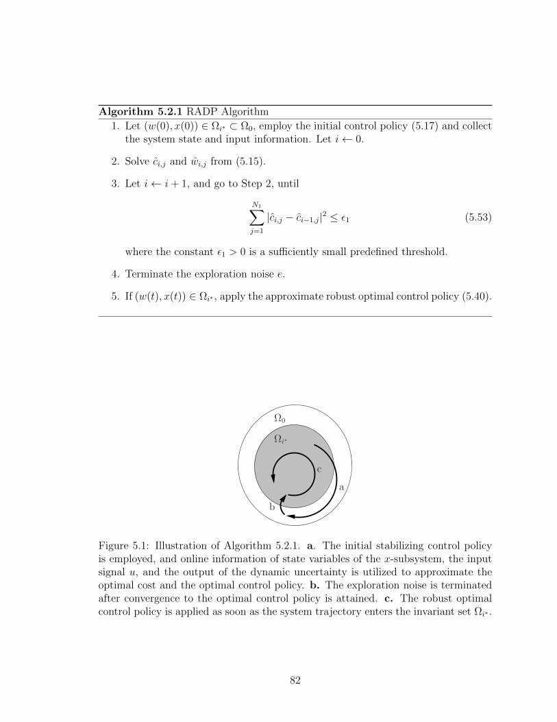
Algorithm 5.2.1 RADP Algorithm
1. Let (w(0), x(0)) ∈ Ωi∗ ⊂ Ω0, employ the initial control policy (5.17) and collectthe system state and input information. Let i← 0.
2. Solve ci,j and wi,j from (5.15).
3. Let i← i+ 1, and go to Step 2, until
N1∑
j=1
|ci,j − ci−1,j|2 ≤ ε1 (5.53)
where the constant ε1 > 0 is a sufficiently small predefined threshold.
4. Terminate the exploration noise e.
5. If (w(t), x(t)) ∈ Ωi∗ , apply the approximate robust optimal control policy (5.40).
Ω0
Ωi∗
a
b
c
Figure 5.1: Illustration of Algorithm 5.2.1. a. The initial stabilizing control policyis employed, and online information of state variables of the x-subsystem, the inputsignal u, and the output of the dynamic uncertainty is utilized to approximate theoptimal cost and the optimal control policy. b. The exploration noise is terminatedafter convergence to the optimal control policy is attained. c. The robust optimalcontrol policy is applied as soon as the system trajectory enters the invariant set Ωi∗ .
82

5.3 RADP with unmatched dynamic uncertainty
In this section, we extend the RADP methodology to nonlinear systems with un-
matched dynamic uncertainties. To begin with, consider the system:
w = ∆w(w, x) (5.54)
x = f(x) + g(x) [z + ∆(w, x)] (5.55)
z = f1(x, z) + u+ ∆1(w, x, z) (5.56)
where [xT , z]T ∈ Rn×R is the measured component of the state available for feedback
control; w, u, ∆w, f , g, and ∆ are defined in the same way as in (5.8)-(5.9); f1 :
Rn × R → R and ∆1 : Rp × Rn × R → R are locally Lipschitz functions and are
assumed to be unknown.
Assumption 5.3.1. There exist class K functions κ5, κ6, κ7, such that the following
inequality holds:
|∆1(w, x, z)| ≤ maxκ5 (|w|) , κ6 (|x|) , κ7 (|z|). (5.57)
5.3.1 Online learning
Let us define a virtual control policy ξ = uro, where uro is the same as in (5.40).
Then, a state transformation can be performed as ζ = z − ξ. Along the trajectories
of (5.55)-(5.56), it follows that
ζ = f1(x, z) + u+ ∆1 − g1(x)∆ (5.58)
83

where f1(x, z) = f1(x, z)− ∂ξ∂xf(x)− ∂ξ
∂xg(x)z, and g1(x) = ∂ξ
∂xg(x). By approximation
theory [126], f1(x, z) and g1(x) can be approximated by:
f1(x, z) =
N3∑
j=1
wf,jψj(x, z), (5.59)
g1(x) =
N4−1∑
j=0
wg,jφj(x) (5.60)
where ψj(x, z)∞j=1 is a sequence of linearly independent basis functions on some
compact set Ω1 ∈ Rn+1 containing the origin as its interior, φ0(x) ≡ 1, wf,j and wg,j
are constant weights to be trained. As in the matched case, a similar assumption on
the initial control policy is given as follows.
Assumption 5.3.2. The closed-loop system composed of (5.54)-(5.56), and
u = u0(x, z) + e (5.61)
is ISS when e, the exploration noise, is considered to be the input.
Under Assumption 5.3.2, we can find an invariant set Ω1,0 for the closed-loop
system composed of (5.54)-(5.56) and (5.61), and approximate the unknown functions
on the set
Ω1 = (x, z) : ∃w, s.t.(w, x, z) ∈ Ω1,0. (5.62)
Then, we give the following two-phase learning scheme.
84
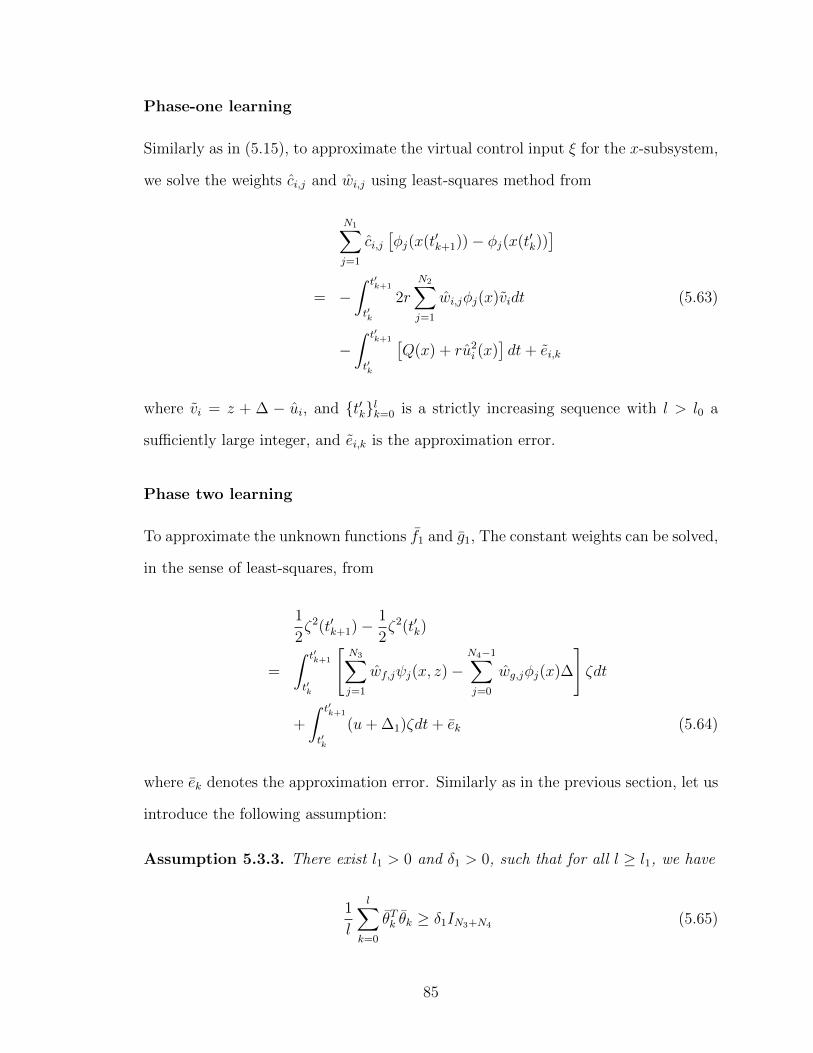
Phase-one learning
Similarly as in (5.15), to approximate the virtual control input ξ for the x-subsystem,
we solve the weights ci,j and wi,j using least-squares method from
N1∑
j=1
ci,j[φj(x(t′k+1))− φj(x(t′k))
]
= −∫ t′k+1
t′k
2r
N2∑
j=1
wi,jφj(x)vidt (5.63)
−∫ t′k+1
t′k
[Q(x) + ru2
i (x)]dt+ ei,k
where vi = z + ∆ − ui, and t′klk=0 is a strictly increasing sequence with l > l0 a
sufficiently large integer, and ei,k is the approximation error.
Phase two learning
To approximate the unknown functions f1 and g1, The constant weights can be solved,
in the sense of least-squares, from
1
2ζ2(t′k+1)− 1
2ζ2(t′k)
=
∫ t′k+1
t′k
[N3∑
j=1
wf,jψj(x, z)−N4−1∑
j=0
wg,jφj(x)∆
]ζdt
+
∫ t′k+1
t′k
(u+ ∆1)ζdt+ ek (5.64)
where ek denotes the approximation error. Similarly as in the previous section, let us
introduce the following assumption:
Assumption 5.3.3. There exist l1 > 0 and δ1 > 0, such that for all l ≥ l1, we have
1
l
l∑
k=0
θTk θk ≥ δ1IN3+N4 (5.65)
85
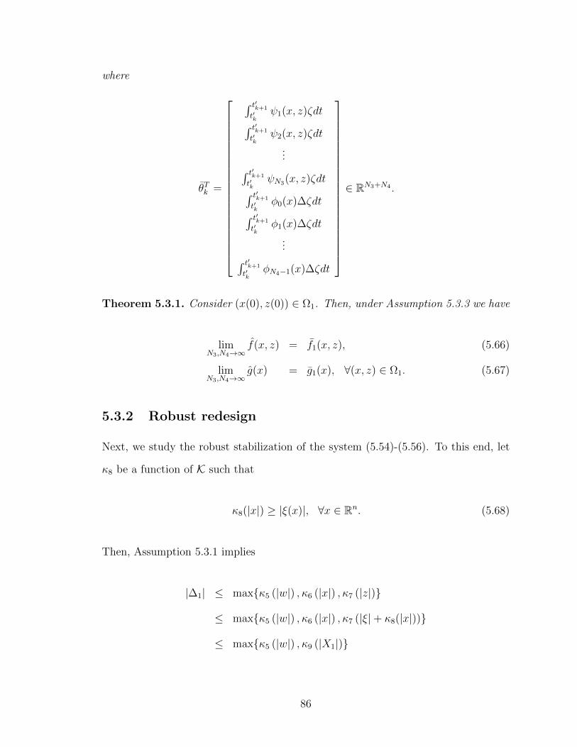
where
θTk =
∫ t′k+1
t′kψ1(x, z)ζdt
∫ t′k+1
t′kψ2(x, z)ζdt
...∫ t′k+1
t′kψN3(x, z)ζdt
∫ t′k+1
t′kφ0(x)∆ζdt
∫ t′k+1
t′kφ1(x)∆ζdt
...∫ t′k+1
t′kφN4−1(x)∆ζdt
∈ RN3+N4 .
Theorem 5.3.1. Consider (x(0), z(0)) ∈ Ω1. Then, under Assumption 5.3.3 we have
limN3,N4→∞
f(x, z) = f1(x, z), (5.66)
limN3,N4→∞
g(x) = g1(x), ∀(x, z) ∈ Ω1. (5.67)
5.3.2 Robust redesign
Next, we study the robust stabilization of the system (5.54)-(5.56). To this end, let
κ8 be a function of K such that
κ8(|x|) ≥ |ξ(x)|, ∀x ∈ Rn. (5.68)
Then, Assumption 5.3.1 implies
|∆1| ≤ maxκ5 (|w|) , κ6 (|x|) , κ7 (|z|)
≤ maxκ5 (|w|) , κ6 (|x|) , κ7 (|ξ|+ κ8(|x|))
≤ maxκ5 (|w|) , κ9 (|X1|)
86
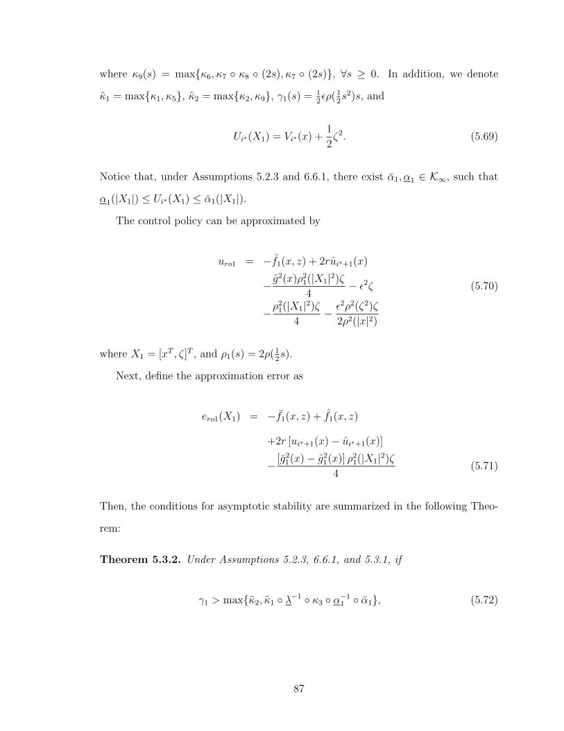
where κ9(s) = maxκ6, κ7 κ8 (2s), κ7 (2s), ∀s ≥ 0. In addition, we denote
κ1 = maxκ1, κ5, κ2 = maxκ2, κ9, γ1(s) = 12ερ(1
2s2)s, and
Ui∗(X1) = Vi∗(x) +1
2ζ2. (5.69)
Notice that, under Assumptions 5.2.3 and 6.6.1, there exist α1, α1 ∈ K∞, such that
α1(|X1|) ≤ Ui∗(X1) ≤ α1(|X1|).
The control policy can be approximated by
uro1 = −f1(x, z) + 2rui∗+1(x)
− g2(x)ρ2
1(|X1|2)ζ
4− ε2ζ (5.70)
−ρ21(|X1|2)ζ
4− ε2ρ2(ζ2)ζ
2ρ2(|x|2)
where X1 = [xT , ζ]T , and ρ1(s) = 2ρ(12s).
Next, define the approximation error as
ero1(X1) = −f1(x, z) + f1(x, z)
+2r [ui∗+1(x)− ui∗+1(x)]
− [g21(x)− g2
1(x)] ρ21(|X1|2)ζ
4(5.71)
Then, the conditions for asymptotic stability are summarized in the following Theo-
rem:
Theorem 5.3.2. Under Assumptions 5.2.3, 6.6.1, and 5.3.1, if
γ1 > maxκ2, κ1 λ−1 κ3 α−11 α1, (5.72)
87

and if the following implication holds for some constant d1 > 0:
0 < Ui∗(X1) ≤ d1 ⇒ max|ero1(X1)|, |ero(x)| < γ1(|X1|),
then the closed-loop system comprised of (5.54)-(5.56), and (5.70) is asymptotically
stable at the origin. In addition, there exists σ1 ∈ K∞, such that
Ω1,i∗ = (w,X1) : max [σ1(Ui∗(X1)),W (w)] ≤ σ1(d1)
is an estimate of the region of attraction.
Proof. Define
ero1(X1) =
ero1(X1), Ui∗(X1) ≤ d1,
0, Ui∗(X1) > d1,
¯ero(x) =
ero(x), Ui∗(X1) ≤ d1,
0, Ui∗(X1) > d1,
Along the solutions of (5.54)-(5.56) with the control policy
u = −f1(x, z) + 2rui∗+1(x)− g2(x)ρ21(|X1|2)ζ
4
−ρ21(|X1|2)ζ
4− ε2ρ2(ζ2)ζ
2ρ2(|x|2)− ε2ζ − ero1(X1),
88

it follows that
Ui∗ ≤ −Q0(x)− 1
2ε2ζ2
−γ21(|X1|)−maxκ2
1(|w|), κ22(|X1|), ¯e2
ro(x)14ρ2(|x|2)
−γ21(|X1|)−maxκ2
1(|w|), κ22(|X1|), ¯e2
ro(x)14ρ2
1(|X1|2)
−γ21(|X1|)−maxκ2
1(|w|), κ22(|X1|), e2
ro1(X1)14ρ2
1(|X1|2)
As a result,
Ui∗(X1) ≥ α1 γ−11 κ1 λ−1(W (w))
⇒ Ui∗ ≤ −Q0(x)− 12ε2|ζ|2.
The rest of the proof follows the same reasoning as in the proof of Theorem
5.2.2.
Remark 5.3.1. In the absence of the dynamic uncertainty (i.e., ∆ = 0, ∆1 = 0 and
the w-system is absent), the smooth functions ρ and ρ1 can all be replaced by 0, and
the system becomes
X1 = F1(X1) +G1uo1 (5.73)
where F1(X1) =
f(x) + g(x)ζ + g(x)ξ
−∇Vi∗(x)Tg(x)
, G1 =
0
1
, and uo1 = −ε2ζ2. As a
result, it can be concluded that the control policy u = uo1 is an approximate optimal
control policy with respect to the cost functional
J1(X1(0);u) =
∫ ∞
0
[Q1 (x, ζ) +
1
2ε2u2
]dt (5.74)
89
with X1(0) = [xT0 , z0 − ui∗(x0)]T and Q1 (x, ζ) = Q (x) + 14r
[∇Vi∗(x)Tg(x)
]2+ ε2
2ζ2.
Remark 5.3.2. Like in the matched case, by selecting large enough d1 in Theorem
5.3.2, semi-global stabilization is achieved.
5.3.3 The RADP algorithm with unmatched dynamic uncer-
tainty
The RADP algorithm with unmatched dynamic uncertainty is given in Algorithm
5.3.1.
Algorithm 5.3.1 RADP Algorithm
1. Let (w(0), x(0), z(0)) ∈ Ω1,i∗ ⊂ Ω1,0, employ the initial control policy (5.61) andcollect the system state and input information. Let i← 0.
2. Solve ci,j and wi,j from (5.63).
3. Let i← i+ 1, and go to Step 2, until
N1∑
j=1
|ci,j − ci−1,j|2 ≤ ε1 (5.75)
where the constant ε1 > 0 is a sufficiently small predefined threshold.
4. Solve wf,j and wg,j from (5.64).
5. Terminate the exploration noise e.
6. If (w(t), x(t), z(t)) ∈ Ω1,i∗ , apply the approximate robust optimal control policy(5.70).
5.4 Numerical examples
In this section, we apply the proposed online RADP schemes to the design of robust
optimal control policies for a jet engine and a one-machine power system.
90
5.4.1 Jet engine
Consider the following dynamic model for jet engine surge and stall [119], [95] de-
scribed by
Φ = −Ψ + ΨC(Φ)− 3ΦR (5.76)
Ψ =1
β2(Φ− ΦT (Ψ)) (5.77)
R = σR(1− Φ2 −R
)(5.78)
where Φ is the scaled annulus-averaged flow, Ψ is the plenum pressure rise, and
R > 0 is the normalized rotating stall amplitude. Functions ΦC(Φ) and ΦT (Ψ) are
the compressor and throttle characteristics, respectively. According to [119], ΦT is
assumed to take the form of
ΦT (Ψ) = γ√
Ψ− 1 (5.79)
and ΨC(Φ) is assumed to be satisfying ΨC(0) = 1+ΨC0 with ΨC0 a constant describing
the shut-off pressure rise. The equilibrium of the system is
Re = 0,Φe = 1,Ψe = ΨC(Φe) = ΨeC0 + 2.
Performing the following state and input transformations [95]
φ = Φ− Φe (5.80)
ψ = Ψ−Ψe (5.81)
u =1
β2
[φ− β2γ
√ψ + ΨC0 + 2 + 2
], (5.82)
91
system (5.76)-(5.78) can be converted to
R = −σR2 − σR(2φ+ φ2
), R(0) ≥ 0 (5.83)
φ = ΨC(φ+ 1)− 2−ΨC0
− (ψ + 3Rφ+ 3R) (5.84)
ψ = u (5.85)
Notice that this system is in the form of (5.54)-(5.56), if we choose w = R, x = φ,
and z = ψ. The function ΨC and the constant σ are assumed to be uncertain, but
satisfy
−1
2φ3 − 2φ2 ≤ ΨC(s+ 1)− 2−ΨC0 ≤ −
1
2φ3 (5.86)
and 0.1 < σ < 1. The initial stabilizing policy and the initial virtual control policies
are selected to be u = 6φ− 2ψ and ψ = 3φ, with V (R, φ, ψ) = R+ 12φ2 + 1
2(ψ − 3φ)2
a Lyapunov function of the closed-loop system.
For simulation purpose, we set σ = 0.3, β = 0.702, ΨC0 = 1.7, and ΨC(φ + 1) =
ΨC0 + 2 − 32φ2 − 1
2φ3 [119]. We set Q(φ) = 4(φ2 + φ3 + φ4), and r = 1. For robust
redesign, we set ρ(s) = 0.01s. The basis functions are selected to be polynomials
of φ and ψ with order less or equal to four. The exploration noise is set to be
e = 10 cos(0.1t).
The RADP learning started from the beginning of the simulation and finished at
t = 10s, when the control policy is updated after six iterations and the convergence
criterion (5.75) in Algorithm 1 with ε1 = 10−6 is satisfied. The approximated cost
functions before and after phase-one learning are shown in Figure 5.2. The plots of
state trajectories of the closed-loop system are shown in Figures 5.3-5.5.
92
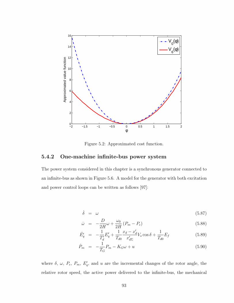
−2 −1.5 −1 −0.5 0 0.5 1 1.5 20
2
4
6
8
10
12
14
16
φ
Ap
pro
xim
ate
d v
alu
e f
un
ctio
n
V0(φ)
V6(φ)
Figure 5.2: Approximated cost function.
5.4.2 One-machine infinite-bus power system
The power system considered in this chapter is a synchronous generator connected to
an infinite-bus as shown in Figure 5.6. A model for the generator with both excitation
and power control loops can be written as follows [97]:
δ = ω (5.87)
ω = − D
2Hω +
ω0
2H(Pm − Pe) (5.88)
E ′q = − 1
T ′dE ′q +
1
Td0
xd − x′dx′dΣ
Vs cos δ +1
Td0
Ef (5.89)
Pm = − 1
TGPm −KGω + u (5.90)
where δ, ω, Pe, Pm, E ′q, and u are the incremental changes of the rotor angle, the
relative rotor speed, the active power delivered to the infinite-bus, the mechanical
93
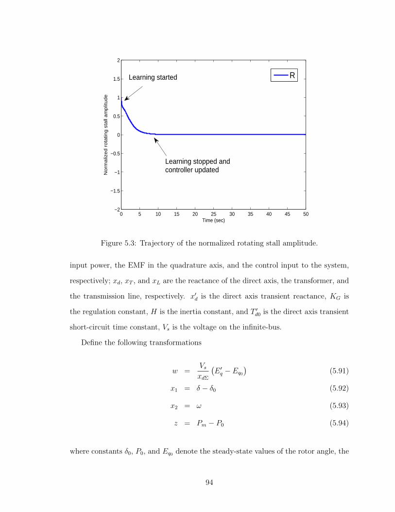
0 5 10 15 20 25 30 35 40 45 50−2
−1.5
−1
−0.5
0
0.5
1
1.5
2
Time (sec)
No
rma
lize
d r
ota
ting
sta
ll a
mp
litu
de
RLearning started
Learning stopped andcontroller updated
Figure 5.3: Trajectory of the normalized rotating stall amplitude.
input power, the EMF in the quadrature axis, and the control input to the system,
respectively; xd, xT , and xL are the reactance of the direct axis, the transformer, and
the transmission line, respectively. x′d is the direct axis transient reactance, KG is
the regulation constant, H is the inertia constant, and T ′d0 is the direct axis transient
short-circuit time constant, Vs is the voltage on the infinite-bus.
Define the following transformations
w =VsxdΣ
(E ′q − Eq0
)(5.91)
x1 = δ − δ0 (5.92)
x2 = ω (5.93)
z = Pm − P0 (5.94)
where constants δ0, P0, and Eq0 denote the steady-state values of the rotor angle, the
94
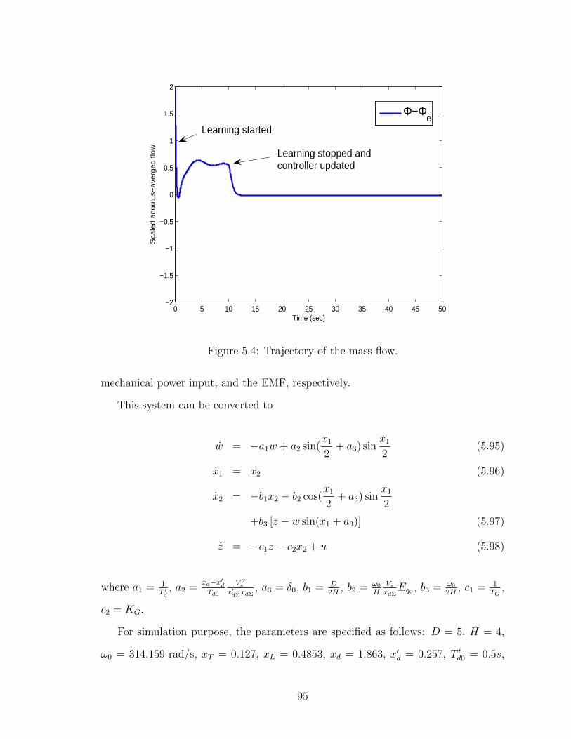
0 5 10 15 20 25 30 35 40 45 50−2
−1.5
−1
−0.5
0
0.5
1
1.5
2
Time (sec)
Sca
led
an
uu
lus−
ave
rge
d f
low
Φ−Φe
Learning stopped andcontroller updated
Learning started
Figure 5.4: Trajectory of the mass flow.
mechanical power input, and the EMF, respectively.
This system can be converted to
w = −a1w + a2 sin(x1
2+ a3) sin
x1
2(5.95)
x1 = x2 (5.96)
x2 = −b1x2 − b2 cos(x1
2+ a3) sin
x1
2
+b3 [z − w sin(x1 + a3)] (5.97)
z = −c1z − c2x2 + u (5.98)
where a1 = 1T ′d
, a2 =xd−x′dTd0
V 2s
x′dΣxdΣ, a3 = δ0, b1 = D
2H, b2 = ω0
HVsxdΣ
Eq0 , b3 = ω0
2H, c1 = 1
TG,
c2 = KG.
For simulation purpose, the parameters are specified as follows: D = 5, H = 4,
ω0 = 314.159 rad/s, xT = 0.127, xL = 0.4853, xd = 1.863, x′d = 0.257, T ′d0 = 0.5s,
95
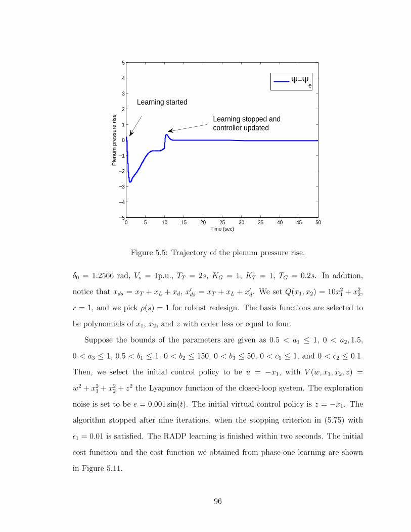
0 5 10 15 20 25 30 35 40 45 50−5
−4
−3
−2
−1
0
1
2
3
4
5
Time (sec)
Ple
nu
m p
ress
ure
ris
e
Ψ−Ψe
Learning started
Learning stopped andcontroller updated
Figure 5.5: Trajectory of the plenum pressure rise.
δ0 = 1.2566 rad, Vs = 1p.u., TT = 2s, KG = 1, KT = 1, TG = 0.2s. In addition,
notice that xds = xT + xL + xd, x′ds = xT + xL + x′d. We set Q(x1, x2) = 10x2
1 + x22,
r = 1, and we pick ρ(s) = 1 for robust redesign. The basis functions are selected to
be polynomials of x1, x2, and z with order less or equal to four.
Suppose the bounds of the parameters are given as 0.5 < a1 ≤ 1, 0 < a2, 1.5,
0 < a3 ≤ 1, 0.5 < b1 ≤ 1, 0 < b2 ≤ 150, 0 < b3 ≤ 50, 0 < c1 ≤ 1, and 0 < c2 ≤ 0.1.
Then, we select the initial control policy to be u = −x1, with V (w, x1, x2, z) =
w2 + x21 + x2
2 + z2 the Lyapunov function of the closed-loop system. The exploration
noise is set to be e = 0.001 sin(t). The initial virtual control policy is z = −x1. The
algorithm stopped after nine iterations, when the stopping criterion in (5.75) with
ε1 = 0.01 is satisfied. The RADP learning is finished within two seconds. The initial
cost function and the cost function we obtained from phase-one learning are shown
in Figure 5.11.
96
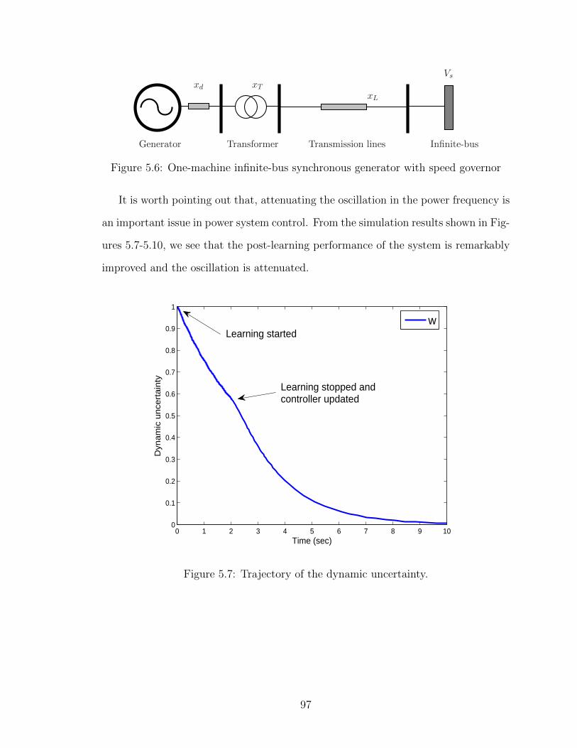
TransformerGenerator Transmission lines Infinite-bus
Vs
xL
xTxd
Figure 5.6: One-machine infinite-bus synchronous generator with speed governor
It is worth pointing out that, attenuating the oscillation in the power frequency is
an important issue in power system control. From the simulation results shown in Fig-
ures 5.7-5.10, we see that the post-learning performance of the system is remarkably
improved and the oscillation is attenuated.
0 1 2 3 4 5 6 7 8 9 100
0.1
0.2
0.3
0.4
0.5
0.6
0.7
0.8
0.9
1
Time (sec)
Dyn
am
ic u
nce
rta
inty
wLearning started
Learning stopped andcontroller updated
Figure 5.7: Trajectory of the dynamic uncertainty.
97
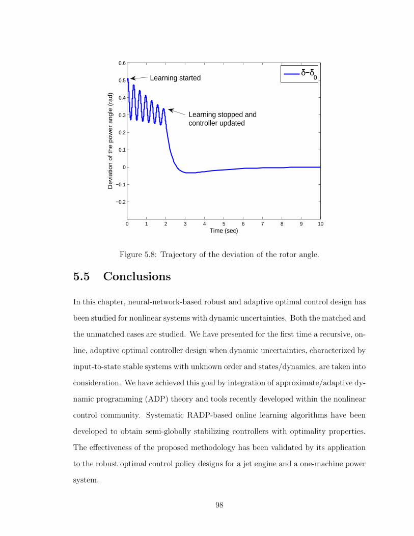
0 1 2 3 4 5 6 7 8 9 10
−0.2
−0.1
0
0.1
0.2
0.3
0.4
0.5
0.6
Time (sec)
De
via
tion
of
the
po
we
r a
ng
le (
rad
)
δ−δ0Learning started
Learning stopped andcontroller updated
Figure 5.8: Trajectory of the deviation of the rotor angle.
5.5 Conclusions
In this chapter, neural-network-based robust and adaptive optimal control design has
been studied for nonlinear systems with dynamic uncertainties. Both the matched and
the unmatched cases are studied. We have presented for the first time a recursive, on-
line, adaptive optimal controller design when dynamic uncertainties, characterized by
input-to-state stable systems with unknown order and states/dynamics, are taken into
consideration. We have achieved this goal by integration of approximate/adaptive dy-
namic programming (ADP) theory and tools recently developed within the nonlinear
control community. Systematic RADP-based online learning algorithms have been
developed to obtain semi-globally stabilizing controllers with optimality properties.
The effectiveness of the proposed methodology has been validated by its application
to the robust optimal control policy designs for a jet engine and a one-machine power
system.
98
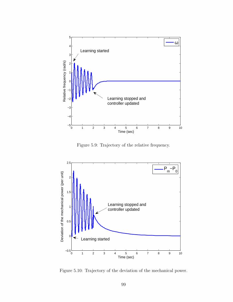
0 1 2 3 4 5 6 7 8 9 10−5
−4
−3
−2
−1
0
1
2
3
4
5
Time (sec)
Re
lativ
e f
req
ue
ncy
(ra
d/s
)
ω
Learning started
Learning stopped andcontroller updated
Figure 5.9: Trajectory of the relative frequency.
0 1 2 3 4 5 6 7 8 9 10−0.5
0
0.5
1
1.5
2
2.5
Time (sec)
De
via
tion
of
the
me
cha
nic
al p
ow
er
(pe
r u
nit)
Pm
−P0
Learning started
Learning stopped andcontroller updated
Figure 5.10: Trajectory of the deviation of the mechanical power.
99

−2
−1
0
1
2
−3−2
−10
12
3
0
50
100
150
200
250
300
350
400
δ−δ0
w
App
roxi
mat
ed v
alue
func
tion
V9V0
Figure 5.11: Approximated cost function.
100
Chapter 6
Global robust adaptive dynamic
programming via
sum-of-squares-programming
In the previous section, neural networks are employed to achieve online approximation
of the cost function and the control policy. Actually, neural networks are widely used
in the previous ADP architecture. However, although they can be used as universal
approximators [57], [124], there are at least two major limitations for ADP-based
online implementations. First, in order to approximate unknown functions with high
accuracy, a large number of basis functions comprising the neural network are usually
required. Hence, it may incur a huge computational burden for the learning system.
Besides, it is not trivial to specify the type of basis functions, when the target function
to be approximated is unknown. Second, neural network approximations generally
are effective only on some compact sets, but not in the entire state space. Therefore,
the resultant control policy may not provide global asymptotic stability for the closed-
loop system. In addition, the compact set, on which the uncertain functions of interest
are to be approximated, has to be carefully quantified before one applies the online
101
learning method, such that stability can be assured during the learning process [75].
The main purpose of this chapter is to develop a novel RADP methodology to
achieve global and adaptive suboptimal stabilization of uncertain continuous-time
nonlinear system via online learning. As the first contribution of this chapter, an op-
timization problem, of which the solutions can be easily parameterized, is proposed
to relax the problem of solving the Hamilton-Jacobi-Bellman (HJB) equation. This
approach is similar to the relaxation method used in approximate dynamic program-
ming for Markov decision processes (MDPs) with finite state space [32], and more
generalized discrete-time systems [106, 178, 179, 137, 139, 153]. However, methods
developed in these papers cannot be trivially extended to the continuous-time set-
ting, or achieve global asymptotic stability of general nonlinear systems. The idea of
relaxation was also used in nonlinear H∞ control, where Hamilton-Jacobi inequalities
are used for nonadaptive systems [52, 169].
The second contribution of the chapter is to propose a relaxed policy iteration
method. For polynomial systems, we formulate each iteration step of the proposed
policy iteration as a sum of squares (SOS) program [125, 17], and give its equivalent
semidefinite programming (SDP) problem [170]. For nonlinear functions that cannot
be parameterized using a basis of polynomials, a less conservative sufficient condition
is derived to decide their non-negativity by examining the coefficients. Thus, the
proposed policy iteration is formulated as a more general SDP problem. It is worth
pointing out that, different from the inverse optimal control design [96], the proposed
method finds directly a suboptimal solution to the original optimal control problem.
The third contribution is an online learning method that implements the proposed
iterative schemes using only the real-time online measurements, when the perfect sys-
tem knowledge is not available. This method can be regarded as a nonlinear variant
of our recent work for continuous-time linear systems with completely unknown sys-
tem dynamics [68]. This method distinguishes from previously known nonlinear ADP
102
methods in that the neural network approximation is avoided for computational bene-
fits and that the resultant control policy is globally stabilizing, instead of semiglobally
or locally stabilizing.
The fourth contribution of this chapter is the robust redesign of the approximate
suboptimal control policy, such that the overall system can be globally asymptotically
stable in the presence of dynamic uncertainties. As in the previous chapter, the key
strategy is to integrate the idea of gain assignment [83, 129] and the Lyapunov-based
small-gain theorem [80] in nonlinear control theory.
The remainder of this chapter is organized as follows. 6.1 formulates the problem
and introduces some basic results in nonlinear optimal control and nonlinear optimiza-
tion. Section 6.2 relaxes the problem of solving an HJB equation to an optimization
problem. Section 6.3 develops a relaxed policy iteration technique for polynomial
systems based on sum of squares (SOS) programming [17]. Section 6.4 develops an
online learning method for applying the proposed policy iteration, when the system
dynamics are not known exactly. Section 6.5 extends the proposed method to deal
with more generalized nonlinear systems. Section 6.6 develops a way to redesign the
suboptimal control policy. Section 6.7 examines three numerical examples to validate
the efficiency and effectiveness of the proposed method. Section 6.8 gives concluding
remarks.
6.1 Problem formulation and preliminaries
In this section, we first formulate the control problem to be studied in the chapter.
Then, we introduce some basic tools in nonlinear optimal control and optimization
theories, based on which our main results in this chapter will be developed.
103
6.1.1 Problem formulation
Consider the nonlinear system
x = f(x) + g(x)u (6.1)
where x ∈ Rn is the system state, u ∈ Rm is the control input, f(x) and g(x) are
locally Lipschitz functions with f(0) = 0.
In conventional optimal control theory [103], the common objective is to find a
control policy u that minimizes certain performance index. In this chapter, it is
specified as follows.
J(x0, u) =
∫ ∞
0
r(x(t), u(t))dt, x(0) = x0 (6.2)
where r(x, u) = Q(x) + uTRu, with Q(x) a positive definite function, and R is a
symmetric positive definite matrix. Notice that, the purpose of specifying r(x, u) in
this form is to guarantee that an optimal control policy can be explicitly determined,
if it exists.
Assumption 6.1.1. Consider system (6.1). There exist a function V0 ∈ P and a
feedback control policy u1, such that
L(V0(x), u1(x)) ≥ 0, ∀x ∈ Rn (6.3)
where, for any V ∈ C1 and u ∈ Rm,
L(V, u) = −∇V T (x)(f(x) + g(x)u)− r(x, u). (6.4)
Under Assumption 6.1.1, the closed-loop system composed of (6.1) and u = u1(x)
is globally asymptotically stable at the origin, with a well-defined Lyapunov function
104

V0. With this property, u1 is also known as an admissible control policy [6], implying
that the cost J(x0, u1) is finite, ∀x0 ∈ Rn. Indeed, integrating both sides of (6.3)
along the trajectories of the closed-loop system composed of (6.1) and u = u1(x) on
the interval [0,+∞), it is easy to show that
J(x0, u1) ≤ V0(x0), ∀x0 ∈ Rn. (6.5)
6.1.2 Optimality and stability
Here, we recall a basic result connecting optimality and global asymptotic stability
in nonlinear systems [141]. To begin with, let us give the following assumption.
Assumption 6.1.2. There exists V o ∈ P, such that the Hamilton-Jacobi-Bellman
(HJB) equation holds
H(V o) = 0 (6.6)
where
H(V ) = ∇V T (x)f(x) +Q(x)− 1
4∇V T (x)g(x)R−1gT (x)∇V (x).
Under Assumption 6.1.2, it is easy to see that V o is a well-defined Lyapunov
function for the closed-loop system comprised of (6.1) and
uo(x) = −1
2R−1gT (x)∇V o(x). (6.7)
Hence, this closed-loop system is globally asymptotically stable at x = 0 [86].
Then, according to [141, Theorem 3.19], uo is the optimal control policy, and the
105
value function V o(x0) gives the optimal cost at the initial condition x(0) = x0, i.e.,
V o(x0) = minuJ(x0, u) = J(x0, u
o), ∀x0 ∈ Rn. (6.8)
It can also be shown that V o is the unique solution to the HJB equation (9.8)
with V o ∈ P . Indeed, let V ∈ P be another solution to (9.8). Then, by Theorem
3.19 in [141], along the solutions of the closed-loop system composed of (6.1) and
u = u = −12R−1gT∇V , it follows that
V (x0) = V o(x0)−∫ ∞
0
|uo − u|2Rdt, ∀x0 ∈ Rn. (6.9)
Finally, comparing (6.8) and (6.9), we conclude that V o = V .
6.1.3 Conventional policy iteration
The above-mentioned result implies that, if there exists a class-P function which
solves the HJB equation (9.8), an optimal control policy can be obtained. However,
the nonlinear HJB equation (9.8) is almost impossible to be solved analytically in
general. As a result, numerical methods are developed to approximate the solution.
In particular, the following policy iteration method is widely used [136].
Algorithm 6.1.1 Conventional policy iteration
1: Policy evaluation: For i = 1, 2, · · · , solve for the cost function Vi(x) ∈ C1, withVi(0) = 0, from the following partial differential equation.
L(Vi(x), ui(x)) = 0. (6.10)
2: Policy improvement: Update the control policy by
ui+1(x) = −1
2R−1gT (x)∇Vi(x). (6.11)
The following result is a trivial extension of [136, Theorem 4], in which g(x) is a
constant matrix and only stabilization over compact set is considered.
106
Theorem 6.1.1. Suppose Assumptions 6.1.1 and 6.1.2 hold, and the solution Vi(x) ∈
C1 satisfying (6.10) exists, for i = 1, 2, · · · . Let Vi(x) and ui+1(x) be the functions
generated from (6.10) and (6.11). Then, the following properties hold, ∀i = 0, 1, · · · .
1) V o(x) ≤ Vi+1(x) ≤ Vi(x), ∀x ∈ Rn;
2) ui+1 is globally stabilizing;
3) J(x0, ui) is finite, ∀x0 ∈ Rn;
4) Vi(x)∞i=0 and ui(x)∞i=1 converge pointwise to V o(x) and uo(x), respectively.
Notice that finding the analytical solution to (6.10) is still non-trivial. Hence,
in practice, the solution is approximated using, for example, neural networks or
Galerkin’s method [6]. When the precise knowledge of f or g is not available, ADP-
based online approximation method can be applied to compute numerically the cost
functions via online data [172], [75].
In general, approximation methods can only give acceptable results on some com-
pact set in the state space, but cannot be used to achieve global stabilization. In
addition, in order to reduce the approximation error, huge computational complex-
ity is almost inevitable. These facts may affect the effectiveness of the previously
developed ADP-based online learning methods.
6.1.4 Semidefinite programming and sum-of-squares program-
ming
A standard semidefinite programming (SDP) problem can be formulated as the fol-
lowing problem of minimizing a linear function of a variable y ∈ Rn0 subject to a
linear matrix inequality.
107
Problem 6.1.1 (Semidefinite programming [170]).
miny
cTy (6.12)
F0 +
n0∑
i=1
yiFi ≥ 0 (6.13)
where c ∈ Rn0 is a constant column vector, and F0, F1, · · · , Fn0 ∈ Rm0×m0 are
n0 + 1 symmetric constant matrices.
SDPs can be solved using several commercial or non-commercial software pack-
ages, such as the Matlab-based solver CVX [48].
Definition 6.1.1 (Sum of squares [17]). A polynomial p(x) ∈ R[x]0,2d is a sum of
squares (SOS) if there exist q1, q2, · · · , qm0 ∈ R[x]0,d such that
p(x) =m∑
i=1
q2i (x). (6.14)
An SOS programming problem is a convex optimization problem of the following
form
Problem 6.1.2 (SOS programming [17]).
miny
bTy (6.15)
s.t. pi(x; y) are SOS, i = 1, 2, · · · , k0 (6.16)
where pi(x; y) = ai0(x) +∑n0
j=1 aij(x)yj, and aij(x) are given polynomials in R[x]0,2d.
In [17, p.74], it has been pointed out that SOS programs are in fact equivalent
to SDPs. Indeed, the constraints (6.16) are equivalent to the existence of symmetric
matrices Qi ≥ 0 satisfying
pi(x; y) = [x]T0,dQi [x]0,d , i = 1, 2, · · · , k0. (6.17)
108
Then, by extending and matching the coefficients of (6.17), the equations (6.17)
reduce to linear equations between y and the entries of Qi. As a result, Problem 6.1.1
is equivalent to an SDP problem in the variables of y and all the distinct entries of
Qi. This equivalence implies that SOS programs can be reformulated and solved as
SDPs. The conversion from an SOS to an SDP can be performed either manually,
or automatically using, for example, the Matlab toolbox SOSTOOLS [128], YALMIP
[112], and Gloptipoly [53].
6.2 Suboptimal control with relaxed HJB equa-
tion
In general, it is extremely difficult to obtain the analytical solution to the HJB equa-
tion (9.8). Therefore, in this section we consider an auxiliary optimization problem,
which allows us to obtain a suboptimal solution to the minimization problem (9.7)
subject to (6.1). For simplicity, we will omit the arguments of functions whenever
there is no confusion in the context.
Problem 6.2.1 (Relaxed optimal control problem).
minV
∫
Rns(x)V (x)dx (6.18)
s.t. H(V ) ≤ 0 (6.19)
V ∈ P (6.20)
where s(x) is a positive semidefinite function taking positive values only on some
predefined compact set Ω ⊂ Rn.
Remark 6.2.1. Notice that Problem 6.2.1 is called a relaxed problem of (9.8). Indeed,
if we restrict this problem by replacing the inequality constraint (6.19) with the equality
constraint (9.8), there will be only one feasible solution left and the objective function
109

can thus be neglected. As a result, Problem 6.2.1 reduces to the problem of solving
(9.8).
Remark 6.2.2. The function s(x) can also be recognized as the state-relevance weight-
ing function [32]. It is easy to see that better approximation to the optimal cost func-
tion V o in a particular region of state space can be achieved by assigning relatively
higher weights to the region.
Some useful facts about Problem 6.2.1 are given as follows.
Theorem 6.2.1. Under Assumptions 6.1.1 and 6.1.2, the following hold.
1) Problem 6.2.1 has a nonempty feasible set.
2) Let V be a feasible solution to Problem 6.2.1. Then, the control policy
u = −1
2R−1gT∇V (6.21)
is globally stabilizing.
3) For any x0 ∈ Rn, an upper bound of the cost of the closed-loop system comprised
of (6.1) and (6.21) is given by V (x0), i.e.,
J(x0, u) ≤ V (x0). (6.22)
4) Along the trajectories of the closed-loop system (6.1) and (6.21), the following
inequalities hold for any x0 ∈ Rn:
V (x0) +
∫ ∞
0
H(V (x(t)))dt ≤ V o(x0) ≤ V (x0). (6.23)
5) V o as defined in (6.8) is a global optimal solution to Problem 6.2.1.
110
Proof. 1) Define u0 = −1
2R−1gT∇V0. Then,
H(V0) = ∇V T0 (f + gu0) + r(x, u0)
= ∇V T0 (f + gu1) + r(x, u1)
+∇V T0 g(u0 − u1) + |u0|2R − |u1|2R
= ∇V T0 (f + gu1) + r(x, u1)− |u0 − u1|2R
≤ 0
Hence, V0 is a feasible solution to Problem 6.2.1.
2) To show global asymptotic stability, we only need to prove that V is a well-
defined Lyapunov function for the closed-loop system composed of (6.1) and (6.21).
Indeed, along the solutions of the closed-loop system, it follows that
V = ∇V T (f + gu) = H(V )− r(x, u) ≤ −Q(x)
Therefore, the system is globally asymptotically stable at the origin [86].
3) Along the solutions of the closed-loop system comprised of (6.1) and (6.21), we
have
V (x0) = −∫ T
0
∇V T (f + gu)dt+ V (x(T ))
=
∫ T
0
[r(x, u)−H(V )] dt+ V (x(T ))
≥∫ T
0
r(x, u)dt+ V (x(T )) (6.24)
By 2), limT→+∞
V (x(T )) = 0. Therefore, letting T → +∞, by (6.24) and (9.7), we
have
V (x0) ≥ J(x0, u). (6.25)
111
4) By 3), we have
V (x0) ≥ J(x0, u) ≥ minuJ(x0, u) = V o(x0). (6.26)
Hence, the second inequality in (6.23) is proved.
On the other hand,
H(V ) = H(V )−H(V o)
= (∇V −∇V o)T (f + gu) + r(x, u)− (∇V o)Tg(uo − u)− r(x, uo)
= (∇V −∇V o)T (f + gu) + |u− uo|2R
≥ (∇V −∇V o)T (f + gu)
Integrating the above equation along the solutions of the closed-loop system (6.1)
and (6.21) on the interval [0,+∞), we have
V (x0)− V o(x0) ≤ −∫ ∞
0
H(V (x))dt. (6.27)
5) By 3), for any feasible solution V to Problem 6.2.1, we have V o(x) ≤ V (x). So,
∫
Rns(x)V o(x)dx ≤
∫
Rns(x)V (x)dx (6.28)
which implies that V o is a global optimal solution.
The proof is therefore complete.
Remark 6.2.3. A feasible solution V to Problem 6.2.1 may not necessarily be the
true cost function associated with the control policy u defined in (6.21). However, by
Theorem 6.2.1, we see V can be viewed as an upper bound or an overestimate of the
actual cost, inspired by the concept of underestimator in [178]. Further, V serves as
a Lyapunov function for the closed-loop system and can be more easily parameterized
112
than the actual cost function. For simplicity, V is still called the cost function, in the
remainder of the chapter.
6.3 SOS-based policy iteration for polynomial sys-
tems
The inequality constraint (6.19) contained in Problem 6.2.1 provides us the freedom
of specifying desired analytical forms of the cost function. However, solving (6.19) is
non-trivial in general, even for polynomial systems (see, for example, [28], [44], [121],
[147], [197]). Indeed, for any polynomial with degree no less than four, deciding its
non-negativity is an NP-hard problem [125]. Fortunately, due to the developments in
sum of squares (SOS) programming [17, 125], the computational burden can be sig-
nificantly reduced, if inequality constraints can be restricted to SOS constraints. The
purpose of this section is to develop a novel policy iteration method for polynomial
systems using SOS-based methods [17, 125].
6.3.1 Polynomial parametrization
To study polynomial systems, let us first give the following Assumption.
Assumption 6.3.1. There exist integers d > 0, d1 ≥ 0, and r > 0, such that
1. all entries of f(x) belong to R[x]1,d and all entries of g(x) belong to R[x]0,d1;
2. in addition to being positive definite, the weighting function Q(x) satisfies Q(x) ∈
R[x]2,2d;
3. there exist a nonlinear mappings V0 : Rn → R and a feedback control policy
u1 : Rn → Rm, such that V0 ∈ R[x]2,2r ∩ P, u1 ∈ R[x]m1,d, and L(V0, u1) is SOS;
and
113
4. the inequality holds:
d ≥ (2r − 1) + d1. (6.29)
Remark 6.3.1. It is easy to see that, Assumption 6.3.1 holds only if Assumption
6.1.1 holds. In addition, under Assumption 6.3.1, we know that L(V0, u1) ∈ R[x]2,2d.
Indeed, by (6.29), it follows that L(V0, u1) ∈ R[x]2,max(2r−1)+d+(d1+d),2d = R[x]2,2d.
Remark 6.3.2. Notice that the inequality (6.29) can be assumed without loss of
generality. Indeed, if it does not hold, we can always find d > maxd, (2r − 1) + d1.
As a result, Assumption 6.3.1 holds with d replaced by d.
For notational simplicity, we denote the dimensions of [x]1,r, [x]1,d, [x]2,2r, and
[x]2,2d by nr, nd, n2r, and n2d, respectively. By [17], we know nr = (n+rr ) − 1, nd =
(n+dd )− 1, n2r = (n+2r
2r )− n− 1, and n2d = (n+2d2d )− d− 1.
6.3.2 SOS-programming-based policy iteration
Now, we are ready to propose a relaxed policy iteration scheme. Similar as in other
policy-iteration-based iterative schemes, an initial globally stabilizing (and admissi-
ble) control policy has been assumed in Assumption 6.3.1.
Remark 6.3.3. The optimization problem (6.30)-(6.33) is a well defined SOS program
[17]. Indeed, the objective function (6.30) is linear in p, since for any V = pT [x]2,2r,
we have∫Rn s(x)V (x)dx = cTp, with c =
∫Rn s(x)[x]2,2rdx. In addition, notice that
since the objective function is nonnegative, its optimal value must be finite.
Theorem 6.3.1. Under Assumptions 6.1.2 and 6.3.1, the following are true, for
i = 1, 2, · · · .
1) The SOS program (6.30)-(6.33) has a nonempty feasible set.
114
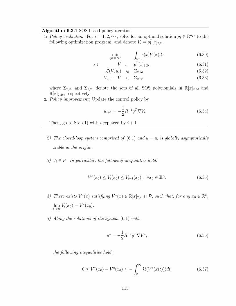
Algorithm 6.3.1 SOS-based policy iteration
1: Policy evaluation: For i = 1, 2, · · · , solve for an optimal solution pi ∈ Rn2r to thefollowing optimization program, and denote Vi = pTi [x]2,2r.
minp∈Rn2r
∫
Rns(x)V (x)dx (6.30)
s.t. V := pT [x]2,2r (6.31)
L(V, ui) ∈ Σ2,2d (6.32)
Vi−1 − V ∈ Σ2,2r (6.33)
where Σ2,2d and Σ2,2r denote the sets of all SOS polynomials in R[x]2,2d andR[x]2,2r, respectively.
2: Policy improvement: Update the control policy by
ui+1 = −1
2R−1gT∇Vi. (6.34)
Then, go to Step 1) with i replaced by i+ 1.
2) The closed-loop system comprised of (6.1) and u = ui is globally asymptotically
stable at the origin.
3) Vi ∈ P. In particular, the following inequalities hold:
V o(x0) ≤ Vi(x0) ≤ Vi−1(x0), ∀x0 ∈ Rn. (6.35)
4) There exists V ∗(x) satisfying V ∗(x) ∈ R[x]2,2r ∩ P, such that, for any x0 ∈ Rn,
limi→∞
Vi(x0) = V ∗(x0).
5) Along the solutions of the system (6.1) with
u∗ = −1
2R−1gT∇V ∗, (6.36)
the following inequalities hold:
0 ≤ V ∗(x0)− V o(x0) ≤ −∫ ∞
0
H(V ∗(x(t)))dt. (6.37)
115
Proof. 1) We prove by mathematical induction.
i) Suppose i = 1, under Assumption 6.3.1, we know L(V0, u1) ∈ Σ2,2d. Hence,
V = V0 is a feasible solution to the problem (6.30)-(6.33).
ii) Let uj−1 ∈ R[x]m1,d, and V = Vj−1 be an optimal solution to the problem (6.30)-
(6.33) with i = j − 1 > 1. We show that V = Vj−1 is a feasible solution to the same
problem with i = j.
Indeed, by definition,
uj = −1
2R−1gT∇Vj−1 ∈ R[x]m1,d,
and
L(Vj−1, uj) = −∇V Tj−1(f + guj)− r(x, uj)
= L(Vj−1, uj−1)−∇V Tj−1g(uj − uj−1) + uTj−1Ruj−1 − uTj Ruj
= L(Vj−1, uj−1) + |uj − uj−1|2R.
Under the induction assumption, we know Vj−1 ∈ R[x]2,2r, uj−1 ∈ R[x]m1,d, and
L(Vj−1, uj) ∈ Σ2,2d. Hence, L(Vj−1, uj) ∈ Σ2,2d. As a result, Vj−1 is a feasible solution
to the SOS program (6.30)-(6.33) with i = j.
2) Again, we prove by induction.
i) Suppose i = 1, under Assumption 6.3.1, u1 is globally stabilizing. Also, we can
show that V1 ∈ P . Indeed, for each x0 ∈ Rn with x0 6= 0, we have
V1(x0) ≥∫ ∞
0
r(x, u1)dt > 0. (6.38)
By (6.38) and the constraint (6.33), under Assumption 6.1.2 it follows that
V o ≤ V1 ≤ V0. (6.39)
116
Since both V o and V0 are assumed to belong to P , we conclude that V1 ∈ P .
ii) Suppose ui−1 is globally stabilizing, and Vi−1 ∈ P for i > 1. Let us show that
ui is globally stabilizing, and Vi ∈ P .
Indeed, along the solutions of the closed-loop system composed of (6.1) and u = ui,
it follows that
Vi−1 = ∇V Ti−1(f + gui) = −L(Vi−1, ui)− r(x, ui) ≤ −Q(x).
Therefore, ui is globally stabilizing, since Vi−1 is a well-defined Lyapunov function
for the system. In addition, we have
Vi(x0) ≥∫ ∞
0
r(x, ui)dt > 0, ∀x0 6= 0. (6.40)
Similarly as in (6.39), we can show
V o(x0) ≤ Vi(x0) ≤ Vi−1(x0), ∀x0 ∈ Rn, (6.41)
and conclude that Vi ∈ P .
3) The two inequalities have been proved in (6.41).
4) By 3), for each x ∈ Rn, the sequence Vi(x)∞i=0 is monotonically decreasing
with 0 as its lower bound. Therefore, the limit exists, i.e., there exists V ∗(x), such
that limi→∞
Vi(x) = V ∗(x). Let pi∞i=1 be the sequence such that Vi = pTi [x]2,2r. Then,
we know limi→∞
pi = p∗ ∈ Rn2r , and therefore V ∗ = p∗T [x]2,2r. Also, it is easy to show
V o ≤ V ∗ ≤ V0. Hence, V ∗ ∈ R[x]2,2r ∩ P .
5) By 4), we know
H(V ∗) = −L(V ∗, u∗) ≤ 0, (6.42)
117
which implies that V ∗ is a feasible solution to Problem 6.2.1. Then, the inequalities
in (5) can be obtained by the fourth property in Theorem 6.2.1.
The proof is thus complete.
6.3.3 An equivalent SDP implementation
According to the equivalence between SOS programs and SDPs, the SOS-based policy
iteration can be reformulated as SDPs. Notice that we can always find two linear
mappings ι : Rn2r × Rm×nr → Rn2d and κ : Rn2r → Rm×nr , such that given p ∈ Rn2r
and K ∈ Rm×nr ,
ι(p,K)T [x]2,2d = L(pT [x]2,2r, K[x]1,2r−1) (6.43)
κ(p)T [x]1,2r−1 = −1
2R−1gT∇(pT [x]2,2r) (6.44)
Then, by properties of SOS constraints [17], the polynomial ι(p,K)T [x]2,2d is SOS
if and only if there exists a symmetric and positive semidefinite matrix L ∈ Rnd×nd ,
such that
ι(p,K)T [x]2,2d = [x]T1,dL[x]1,d. (6.45)
Furthermore, there exist linear mappings MP : Rnr×nr → Rn2r and ML : Rnd×nd →
Rn2d , such that, for any vectors p ∈ Rn2r , l ∈ Rn2d , and symmetric matrices P ∈
Rnr×nr and L ∈ Rnd×nd , the following implications are true.
pT [x]2,2r = [x]T1,rP [x]1,r ⇐⇒ p = MP (P ) (6.46)
lT [x]2,2d = [x]T1,dL[x]1,d ⇐⇒ l = ML(L) (6.47)
Under Assumptions 6.1.2 and 6.3.1, the proposed policy iteration can be reformu-
lated as follows.
118
Algorithm 6.3.2 SDP-based policy iteration
1: Let i = 1. Let p0 ∈ Rn2r and K1 ∈ Rm×nd satisfy V0 = pT0 [x]2,2r and u1 = K1[x]1,d.2: Solve for an optimal solution (pi, Pi, Li) ∈ Rn2r×Rnr×nr×Rnd×nd to the following
problem.
minp,P,L
cTp (6.48)
s.t. ι(p,Ki) = ML(L) (6.49)
pi−1 − p = MP (P ) (6.50)
P = P T ≥ 0 (6.51)
L = LT ≥ 0 (6.52)
where c =∫Rn s(x)[x]2,2rdx.
3: Go to Step 2) with Ki+1 = κ(pi) and i replaced by i+ 1.
Remark 6.3.4. The optimization problem (6.48)-(6.52) is a well-defined semidefi-
nite programming (SDP) problem, since it has a linear objective function subject to
linear equality and inequality constraints. It can be directly solved using, for exam-
ple, Matlab-based solver CVX [48]. Also, it can be rewritten in the standard form
(6.12)-(6.13) by equivalently replacing each equality constraint with two inequalities
constraints, and by treating p and entries in P and L as the decision variables.
Corollary 6.3.1. Under Assumptions 6.1.2 and 6.3.1, the following are true.
1. The optimization problem (6.48)-(6.52) has at least one feasible solution, for
i = 1, 2, · · · .
2. Denote Vi = pTi [x]2,2r, ui+1 = Ki[x]1,d, for i = 0, 1, · · · . Then, the sequences
Vi∞i=0 and ui∞i=1 satisfy the properties 2)-5) in Theorem 6.3.1.
Proof. Given pi ∈ Rn2r , there exist Pi and Li such that (pi, Pi, Li) is a feasible solution
to the optimization problem (6.48)-(6.52) if and only if pi is a feasible solution to the
SOS program (6.30)-(6.33). Therefore, by Theorem 6.3.1, 1) holds. In addition, since
the two optimization problems share the identical objective function, we know that
if (pi, Pi, Li) is a feasible solution to the optimization problem (6.48)-(6.52), pi is also
119
an optimal solution to the SOS program (6.30)-(6.33). Hence, the corollary can be
obtained from Theorem 6.3.1.
6.4 Online learning via global adaptive dynamic
programming
The proposed policy iteration method requires the perfect knowledge of the mappings
ι and κ, which can be determined if f and g are known exactly. In practice, precise
system knowledge may be difficult to obtain. Hence, in this section, we develop an
online learning method based on the idea of ADP to implement the iterative scheme
with real-time data, instead of identifying the system dynamics.
To begin with, consider the system
x = f + g(ui + e) (6.53)
where ui is a feedback control policy and e is a bounded time-varying function, known
as the exploration noise, added for the learning purpose.
Lemma 6.4.1. Consider system (6.53). Suppose ui is a globally stabilizing control
policy and there exists Vi−1 ∈ P, such that ∇Vi−1(f + gui) + uTi Rui ≤ 0. Then, the
system (6.53) is forward complete.
Proof. Under Assumptions 6.1.2 and 6.3.1, by Theorem 6.3.1 we know Vi−1 ∈ P .
Then, by completing the squares, it follows that
∇V Ti−1(f + gui + ge) ≤ −uTi Rui − 2uTi Re
= −|ui + e|2R + |e|2R
≤ |e|2R
≤ |e|2R + Vi−1.
120
According to [3, Corollary 2.11], the system (6.53) is forward complete.
By Lemma 6.4.1 and Theorem 6.3.1, we immediately have the following Proposi-
tion.
Proposition 6.4.1. Under Assumptions 6.1.2 and 6.3.1, let ui be a feedback control
policy obtained at the i-th iteration step in the proposed policy iteration algorithm
(6.30)-(6.34) and e be a bounded time-varying function. Then, the closed-loop system
(6.1) with u = ui + e is forward complete.
Suppose there exist p ∈ Rn2r and Ki ∈ Rm×nk such that V = pT [x]2,2r and
ui = Ki[x]1,d. Then, along the solutions of the system (6.53), it follows that
V = ∇V T (f + gui) +∇V TBe
= −r(x, ui)− L(V, ui) +∇V Tge
= −r(x, ui)− L(V, ui) + 2(1
2R−1gT∇V )TRe
= −r(x, ui)− ι(p,Ki)T [x]2,2d − 2[x]T1,dκ(p)TRe (6.54)
where the last row is obtained by (6.43) and (6.44).
Now, integrating the terms in (6.99) over the interval [t, t+ δt], we have
pT ([x(t)]2,2r − [x(t+ δt)]2,2r)
=
∫ t+δt
t
[r(x, ui) + ι(p,Ki)
T [x]2,2d + 2[x]T1,dκ(p)TRe]dt (6.55)
Eq. (6.55) implies that, given p ∈ Rn2r , ι(p,Ki) and κ(p) can be directly calculated
by using real-time online data, without knowing the precise knowledge of f and g.
121
Indeed, define
σe = −[
[x]T2,2d 2[x]T1,d ⊗ eTR]T∈ Rn2d+mnd ,
Φi =
[ ∫ t1,it0,i
σedt∫ t2,it1,i
σedt · · ·∫ tqi,itqi−1,i
σedt
]T∈ Rqi×(n2d+mnd),
Ξi =
[ ∫ t1,it0,i
r(x, ui)dt∫ t2,it1,i
r(x, ui)dt · · ·∫ tqi,itqi−1,i
r(x, ui)dt
]T∈ Rqi ,
Θi =
[[x]2,2r|t1,it0,i [x]2,2r|t2,it1,i · · · [x]2,2r|tqi,itqi−1,i
]T∈ Rqi×n2r .
Then, (6.55) implies
Φi
ι(p,Ki)
vec(κ(p))
= Ξi + Θip. (6.56)
Assumption 6.4.1. For each i = 1, 2, · · · , there exists an integer qi0, such that when
qi ≥ qi0 the following rank condition holds.
rank(Φi) = n2d +mnd. (6.57)
Remark 6.4.1. Such a rank condition (6.57) is in the spirit of persistency of ex-
citation (PE) in adaptive control (e.g. [60, 158]) and is a necessary condition for
parameter convergence.
Given p ∈ Rn2r and Ki ∈ Rm×nd , suppose Assumption 6.4.1 is satisfied and qi ≥ qi0
for all i = 1, 2, · · · . Then, it is easy to see that the values of ι(p,Ki) and κ(p) can be
uniquely determined from
ι(p,Ki)
vec(κ(p))
=
(ΦTi Φi
)−1ΦTi (Ξi + Θip) (6.58)
Now, we are ready to develop the ADP-based online implementation algorithm
122
for the proposed policy iteration method.
Algorithm 6.4.1 Global adaptive dynamic programming algorithm
1: Initialization: Let p0 be the constant vector such that V0 = pT0 [x]2,2r, and leti = 1.
2: Collect online data: Apply u = ui+e to the system and compute the data matricesΦi, Ξi, and Θi, until the rank condition (6.57) in Assumption 6.4.1 is satisfied.
3: Policy evaluation and improvement: Find an optimal solution (pi, Ki+1, Pi, Li) tothe following optimization problem
minp,K,P,L
cTp (6.59)
s.t.
[ML(L)vec(K)
]=
(ΦTi Φi
)−1ΦTi (Ξi + Θip) (6.60)
pi−1 − p = MP (P ) (6.61)
P = P T ≥ 0 (6.62)
L = LT ≥ 0 (6.63)
Then, denote Vi = pTi [x]2,2r, ui+1 = Ki+1[x]1,d, and go to Step 2) with i← i+ 1.
Lemma 6.4.2. Under Assumption 6.4.1, (pi, Ki+1, Pi, Li) is an optimal solution to
the optimization problem (6.59)-(6.63) if and only if (pi, Pi, Li) is an optimal solution
to the optimization problem (6.48)-(6.52) and Ki+1 = κ(pi).
Proof. If (pi, Ki+1, Pi, Li) is an optimal solution to the optimization problem (6.59)-
(6.63), under Assumption 6.4.1, we must have Ki+1 = κ(pi). Then, it is easy to check
(pi, Pi, Li) is a feasible solution to the problem (6.48)-(6.52). On the other hand, if
(pi, Pi, Li) is a feasible solution to the problem (6.48)-(6.52), (pi, κ(pi), Pi, Li) must be
a feasible solution to the problem (6.59)-(6.63). Finally, since the two optimization
problems share the same objective function, their optimal values are the same.
By Lemma 6.4.2 and Theorem 6.3.1, we immediately have the following Theorem.
Theorem 6.4.1. Under Assumptions 6.1.1, 6.3.1 and 6.4.1, the following properties
hold.
1. The optimization problem (6.59)-(6.63) has a nonempty feasible set.
123
2. The sequences Vi∞i=1 and ui∞i=1 satisfy the properties 2)-5) in Theorem 6.3.1.
Remark 6.4.2. Notice that the above-mentioned algorithm assumes that both V0 and
u1 satisfying Assumption 6.3.1 are determined without knowing exactly f and g. In
practice, upper and lower bounds of the coefficients in f and g are often available,
i.e., there exist polynomial mappings f , f , g, g, such that f ≤ f ≤ f and g ≤ g ≤ g.
Thus, it is possible to find a globally stabilizing control policy for interval systems
using robust nonlinear control methods [95, 159]. Then, we can use this control policy
as a candidate of u1 to solve for V0 from the following robust feasibility problem in
SOS programming
−∇V T0 (f + gu1)−Q− uT1Ru1 ∈ Σ2,2d, (6.64)
for all f and g such that f ≤ f ≤ f and g ≤ g ≤ g. This problem, if solvable,
can be converted into a robust linear matrix inequality and efficiently solved using
MATLAB-based solvers, such as the LMI control toolbox [45] or CVX [48].
Remark 6.4.3. In practice, a stopping criterion can be set. For example, the explo-
ration noise can be terminated and ui can be applied as the actual control policy, if
|pi−pi+1| ≤ ε or i = imax, with ε > 0 is a pre-defined threshold and imax a pre-defined
maximum number of iterations.
6.5 Extension to nonpolynomial systems
In this section, we extend the proposed global ADP method to deal with an enlarged
class of nonlinear systems. First, we will give an illustrative example to show that the
SOS condition is conservative for general nonlinear functions. Second, a generalized
parametrization method is proposed. Third, a less conservative sufficient condition
will be derived to assure the non-negativity of a given nonlinear function. Fourth,
124
an SDP-based implementation for the proposed policy iteration technique will be
presented. Finally, an online learning method will be developed.
6.5.1 An illustrative example
The implementation method via SOS programs developed in the previous section
can efficiently handle nonlinear polynomial systems. The results can also be trivially
extended to real trigonometric polynomials [17]. However, the SOS-like constraint
may be conservative to be used as a sufficient condition for non-negativity of general
nonlinear functions. To see this, consider the following illustrative example:
f(x) = ax2 + bx sinx+ c sin2 x =
x
sinx
T
P
x
sinx
. (6.65)
Apparently, a symmetric matrix P can be uniquely determined from the constants a,
b, and c. Similar to the polynomial case, we know f(x) is positive semidefinite, if P
is positive semidefinite. Unfortunately, this condition is very conservative in general.
For example, for the cases of a = 1, b = 0, c = −0.5, or a = 0, b = 1, c = 0,
it is easy to check f(x) is positive semidefinite. But in both cases, we have either
P =
1 0
0 −0.5
or P =
0 0.5
0.5 0
, which are not positive semidefinite matrices.
This illustrative example shows that, instead of searching for a positive semidefi-
nite matrix P , a less conservative sufficient condition for the non-negativity of more
general nonlinear functions is desired. Deriving this condition and developing a glob-
al ADP method for more general nonlinear systems are the main objectives of this
section.
125
6.5.2 Generalized parametrization
Assumption 6.5.1. The function f considered in system (6.1) can be decomposed
as
f = Aσ (6.66)
where A ∈ Rn×l is an uncertain constant matrix, and σ = [σ1(x), σ2(x), · · · , σl(x)]T is
a vector of locally Lipschitz, piecewise-continuous, and linearly independent functions,
satisfying σi(0) = 0, ∀i = 1, 2, · · · , l.
Now, we restrict each feasible solution to Problem 6.2.1 to take the form of V (x) =
φT (x)Pφ(x), where P ∈ Rl×l is a constant matrix and φ = [φ1(x), φ2(x), · · · , φN(x)]T
is a vector of continuously differentiable, linearly independent, functions vanishing at
the origin.
Assumption 6.5.2. The following are true.
1. For each i = 1, 2, · · · , N , j = 1, 2, · · · , N , and k = 1, 2, · · · , n, we have
∂(φiφj)
∂xk∈ spanσ1, σ2, · · · , σl,
2. Let gi be the i-th column of g(x), with i = 1, 2, · · · ,m. Then,
gTi ∇(φiφj) ∈ spanσ1, σ2, · · · , σl.
3. The weighting function Q(x) defined in (9.7) is positive definite and satisfies
Q(x) ∈ spanσ21, σ1σ2, · · · , σiσj, · · · , σ2
l .
Notice that Assumption 6.5.2 is not restrictive, and can be satisfied by expand-
ing the basis functions. Indeed, if 1) and 2) in Assumption 6.5.2 are not satisfied,
126
we can always find locally Lipschitz functions σl+1(x), σl+2(x), · · · , σl+s(x), such
that σ1, σ2, · · · , σl+s are linearly independent and vanish at the origin, satisfying
∂(φiφj)
∂xk∈ spanσ1, σ2, · · · , σl+s and gTi ∇(φiφj) ∈ spanσ1, σ2, · · · , σl+s. Then,
the decomposition (6.66) can be rewritten as
f(x) = Aσ (6.67)
where A = [A 0n×s] and σ = [σ1, σ2, · · · , σl+s]T .
Also, if the intersection between spanσ21, σ1σ2, · · · , σiσj, · · · , σ2
l and the set of
all positive definite functions is empty, we can select Q(x) such that√Q(x) is locally
Lipschitz and positive definite. Define σ = [σ1, σ2, · · · , σl,√Q(x)]. Then, clearly,
all the elements in σ are linearly independent, and the decomposition (6.66) can be
rewritten as f = Aσ, where A =
[A 0n×1
].
6.5.3 A sufficient condition for non-negativity
Define σ1, σ2, · · · , σl1 as the largest linearly independent subset of σ21, σ1σ2, · · · ,
σiσj, · · · , σ2l , and φ1, φ2, · · · , φN1 as the largest linearly independent subset of
φ21, φ1φ2, · · · , φiφj, · · · , φ2
N.
Then, if W ∈ spanφ21, φ1φ2, · · · , φ2
N and δ ∈ spanφ21, σ1σ2, · · · , σ2
l , there exist
uniquely constant vectors p ∈ RN1 and h ∈ Rl1 , such that W = pT φ and δ = hT σ,
where φ = [φ1, φ2, · · · , φN1 ]T and σ = [σ1, σ2, · · · , σl1 ]T .
Using the above-mentioned parametrization method, we now show that it is possi-
ble to decide if W and δ are positive semidefinite functions, by studying the coefficient
vectors p and h.
Without loss of generality, we assume the following properties of φi:
1) For i = 1, 2, · · · , N2, we have φi ≥ 0, with N2 an integer satisfying 1 ≤ N2 ≤ N1.
2) There exist integers ir and jr with r = 1, 2, · · · , N3 , such that 1 ≤ ir, jr ≤ N2,
127
ir 6= jr and φir ≥ φjr .
Definition 6.5.1. For any p ∈ RN1, we say p ∈ S+φ if and only if there exist constants
γ1, γ2, · · · , γN2 ≥ 0, α1, α2, · · · , αN3 ≥ 0, β1, β2, · · · , βN3, and a symmetric positive
semidefinite matrix P ∈ RN×N , such that αi + βi ≥ 0, for i = 1, 2, · · · , N3, and
p = MTφ vec(P ) +
γ1
γ2
...
γN2
0N1−N2
+
N3∑
r=1
0ir−1
αr
0N1−ir
+
0jr−1
βr
0N1−jr
(6.68)
where Mφ ∈ RN2×N1 is a constant matrix satisfying Mφφ = φ⊗ φ.
In addition, W is said to belong to the set S+φ [x] if and only if there exists p ∈ S+
φ ,
such that W = pT φ.
Lemma 6.5.1. If p ∈ S+φ , then pT φ is positive semidefinite.
Proof. By definition, if p ∈ S+φ , it follows that
pT φ = φTPφ+
N2∑
i=1
γ2φi +
N3∑
r=1
(αrφir + βrφjr
)
≥N3∑
r=1
(αrφir − |βr|φjr
)=
N3∑
r=1
(αr − |βr|) φir
≥ 0.
The proof is complete.
In the same way, we can find two sets S+σ and S+
σ [x], such that the following
implications hold
h ∈ S+σ ⇔ hT φ ∈ S+
σ [x]⇒ hT φ ≥ 0. (6.69)
128
6.5.4 Generalized policy iteration
Assumption 6.5.3. There exist p0 ∈ RN1 and K1 ∈ Rm×l1, such that V0 = pT0 φ,
u1 = K1σ, and L(V0, u1) ∈ S+φ .
Remark 6.5.1. Under Assumptions 6.5.1, 6.5.2, and 6.5.3, Assumption 6.1.1 is
satisfied.
Now, let us show how the proposed policy iteration can be practically implement-
ed. First of all, given p ∈ RN1 , since ui = Kiσ, we can always find two linear mappings
ι : RN1 × Rml → Rl1 and κ : RN1 → Rl1×ml , such that
ι(p,K)T σ = L(pT φ,Kiσ) (6.70)
κ(p)T σ = −1
2R−1gT∇(pT φ) (6.71)
Then, under Assumptions 6.1.2, 6.5.1, 6.5.2, and 6.5.3, the proposed policy itera-
tion can be implemented as follows.
Algorithm 6.5.1 SDP-based policy iteration for nonpolynomial systems
1: Initialization:2: Find p0 ∈ RN1 and K1 ∈ Rm×l1 satisfying Assumption 6.5.3, and let i = 1.3: Policy evaluation and improvement:4: Solve for an optimal solution (pi, Ki+1) of the following problem.
minp,K
cTp (6.72)
s.t. ι(p,Ki) ∈ S+σ (6.73)
pi−1 − p ∈ S+φ (6.74)
K = κ(p) (6.75)
where c =∫Rn s(x)φ(x)dx. Then, denote Vi = pTi φ and ui+1 = Ki+1σ.
5: Go to Step 2) with i replaced by i+ 1.
Some useful facts about the above-mentioned policy iteration algorithm are sum-
marized in the following theorem, of which the proof is omitted, because it is nearly
identical to the proof of Theorem 6.3.1.
129
Theorem 6.5.1. Under Assumptions 6.1.2, 6.5.1, 6.5.2, and 6.5.3 the following are
true, for i = 1, 2, · · · .
1) The optimization problem (6.72)-(6.75) has a nonempty feasible set.
2) The closed-loop system comprised of (6.1) and u = ui(x) is globally asymptoti-
cally stable at the origin.
3) Vi ∈ P. In addition, V o(x0) ≤ Vi(x0) ≤ Vi−1(x0), ∀x0 ∈ Rn.
4) There exists p∗ ∈ RN1, such that limi→∞
Vi(x0) = p∗T φ(x0), ∀x0 ∈ Rn.
5) Along the solutions of the system (6.1) with u∗ = −12R−1gT∇(p∗T φ), it follows
that
0 ≤ p∗T φ(x0)− V o(x0) ≤ −∫ ∞
0
H(p∗T φ(x(t)))dt. (6.76)
6.5.5 Online implementation via global adaptive dynamic pro-
gramming
Let V = pT φ. Similar as in Section 6.4, over the interval [t, t+ δt], we have
pT[φ(x(t))− φ(x(t+ δt))
]
=
∫ t+δt
t
[r(x, ui) + ι(p,Ki)
T σ + 2σT κ(p)TRe]dt (6.77)
Therefore, (6.77) shows that, given p ∈ RN1 , ι(p,Ki) and κ(p) can be directly
obtained by using real-time online data, without knowing the precise knowledge of f
and g.
130
Indeed, define
σe = −[σT 2σT ⊗ eTR
]T∈ Rl1+ml,
Φi =
[ ∫ t1,it0,i
σedt∫ t2,it1,i
σedt · · ·∫ tqi,itqi−1,i
σedt
]T∈ Rqi×(l1+ml),
Ξi =
[ ∫ t1,it0,i
r(x, ui)dt∫ t2,it1,i
r(x, ui)dt · · ·∫ tqi,itqi−1,i
r(x, ui)dt
]T∈ Rqi ,
Θi =
[φ(x)|t1,it0,i φ(x)|t2,it1,i · · · φ(x)|tqi,itqi−1,i
]T∈ Rqi×N1 .
Then, (6.77) implies
Φi
ι(p,Ki)
vec(κ(p))
= Ξi + Θip. (6.78)
Assumption 6.5.4. For each i = 1, 2, · · · , there exists an integer qi0, such that, when
qi ≥ qi0, the following rank condition holds.
rank(Φi) = l1 +ml. (6.79)
Let p ∈ RN1 and Ki ∈ Rm×l. Suppose Assumption 6.5.4 holds and assume qi ≥ qi0,
for i = 1, 2, · · · . Then, ι(p,Ki) and κ(p) can be uniquely determined by
h
vec(K)
=
(ΦTi Φi
)−1ΦTi
(Ξi + Θip
). (6.80)
Now, we are ready to develop the ADP-based online implementation algorithm
for the proposed policy iteration method.
Properties of the above algorithm are summarized in the following corollary.
Corollary 6.5.1. Under Assumptions 6.1.2, 6.5.1, 6.5.2, 6.5.3, and 6.5.4, the algo-
rithm enjoys the following properties.
131
Algorithm 6.5.2 Global adaptive dynamic programming algorithm for nonpolyno-mial systems
1: Initialization: Let p0 and K1 satisfying Assumption 6.5.3, and let i = 1.2: Collect online data: Apply u = ui+e to the system and compute the data matrices
Φi, Ξi, and Θi, until the rank condition (6.79) is satisfied.3: Policy evaluation and improvement: Find an optimal solution (pi, hi, Ki+1) to the
following optimization problem
minp,h,K
cTp (6.81)
s.t.
[h
vec(K)
]=
(ΦTi Φi
)−1ΦTi
(Ξi + Θip
)(6.82)
h ∈ S+σ (6.83)
pi−1 − p ∈ S+φ (6.84)
Then, denote Vi = piφ and ui+1 = Ki+1σ.4: Go to Step 2) with i← i+ 1.
1. The optimization problem (6.100)-(6.103) has a feasible solution.
2. The sequences Vi∞i=1 and ui∞i=1 satisfy the properties 2)-5) in Theorem 6.5.1.
6.6 Robust redesign
Consider consider nonlinear system with dynamic uncertainties as follows
w = q(w, x) (6.85)
x = f(x) + g(x) [u+ ∆(w, x)] (6.86)
where x ∈ Rn is the system state, w ∈ Rnw is the state of the dynamic uncertainty,
u ∈ Rm is the control input, f : Rn → Rn and g : Rn → Rn×m are unknown
polynomial mappings with f(0) = 0.
Again, in the presence of the dynamic uncertainty, i.e., the w-subsystem, Algo-
rithm 6.5.2 may not lead to an optimal or suboptimal control policy, since ui obtained
in Algorithm 6.5.2 may not be stabilizing for the overall system (6.85)-(6.86). There-
132
fore, to balance the tradeoff between global robust stability and optimality, here we
develop a method to redesign the control policy. Similarly as in the previous chapter,
the idea is inspired from the work by [83, 129].
To begin with, we define the cost functional as
min J(x0, u) =
∫ ∞
0
[Q(x) + uTRu
]dt, (6.87)
where Q(x) = Q0(x) + ε|x|2, with Q0(x) is a positive definite function, ε > 0 is a
constant, R is a symmetric and positive definite matrix.
Our design objective is twofold. First, we intend to minimize the cost (6.87) for
the nominal system
x = f(x) + g(x)u, (6.88)
by finding online an optimal control policy uo. Second, we want to guarantee the
stability of the system comprised of (6.85) and (6.86) by redesigning the optimal
control policy.
To this end, let us introduce the following Assumption.
Assumption 6.6.1. Consider the system comprised of (6.85) and (6.86). There
exist functions λ, λ ∈ K∞, κ1, κ2, κ3 ∈ K, and positive definite functions W and κ4,
such that for all w ∈ Rp and x ∈ Rn, we have
λ(|w|) ≤ W (w) ≤ λ(|w|), (6.89)
|∆(w, x)| ≤ κ1(|w|) + κ2(|x|), (6.90)
together with the following implication:
W (w) ≥ κ3(|x|)⇒ ∇W (w)T q(w, x) ≤ −κ4(w). (6.91)
133
Assumption 6.6.1 implies that the w-system (6.85) is input-to-state stable (ISS)
[149, 151] when x is considered as the input.
Let Vi ∈ P and ui be the cost function and the control policy obtained from
Algorithm 6.5.2. Then, we know that L(Vi, ui) ≥ 0. Also, there exist α, α ∈ K∞,
such that the following inequalities hold:
α(|x|) ≤ V o(x) ≤ Vi(x) ≤ V0(x) ≤ α(|x|), ∀x0 ∈ Rn; (6.92)
The robustly redesigned control policy is given below:
ur,i = ρ2(|x|2)ui + e (6.93)
where ρ(·) is a smooth and nondecreasing function with ρ(s) ≥ 1, ∀s > 0, e denotes
the time varying exploration noise added for the purpose of online learning.
Theorem 6.6.1. Consider the closed-loop system comprised of (6.85), (6.86), and
(6.93). Let Vi ∈ P and ui be the cost function and the control policy obtained from
Algorithm 6.5.2 at the i-th iteration step. Then, the closed-loop system is ISS with
respect to e as the input, if the following gain condition holds:
γ > κ1 λ−1 κ3 α−1 α + κ2, (6.94)
where γ ∈ K∞ is defined by
γ(s) = εs
√14
+ 12ρ2(s2)
λmin(R). (6.95)
Proof. Let χ1 = κ3 α−1. Then, under Assumption 6.6.1, we immediately have the
134
following implications
W (w) ≥ χ1(Vi(x))
⇒ W (w) ≥ κ3
(α−1(Vi(x))
)≥ κ3 (|x|)
⇒ ∇W (w)T q(w, x) ≤ −κ4(w) (6.96)
Define ρ(x) =√
14
+ 12ρ2(|x|2)
λmin(R). Then, along solutions of the system comprised of
(6.86), it follows that
∇V Ti [f + g (ur,i + ∆)]
≤ −Q(x)− |ui|2R +∇V Ti g[(ρ2(|x|2)− 1
)ui + ∆ + e
]
≤ −Q(x)− ρ2∣∣gT∇Vi
∣∣2 +∇V Ti g (∆ + e)
≤ −Q(x)−∣∣∣∣ρgT∇Vi −
1
2ρ−1∆
∣∣∣∣2
+1
4ρ−2|∆ + e|2
≤ −Q0(x)− ε2|x|2 + ρ−2 max|∆|2, |e|2
≤ −Q0(x)− ρ−2(γ2 −max|∆|2, |e|2
)
Hence, by defining χ2 = α (γ − κ2)−1 κ1 λ−1, it follows that
Vi(x) ≥ maxχ2(W (w)), α (γ − κ2)−1 (|e|)
⇔ Vi(x) ≥ α (γ − κ2)−1 maxκ1 λ−1(W (w)), |e|
⇒ (γ − κ2) α−1 (Vi(x)) ≥ maxκ1 λ−1(W (w)), |e|
⇒ γ(|x|)− κ2(|x|) ≥ maxκ1 λ−1(W (w)), |e|
⇒ γ(|x|)− κ2(|x|) ≥ maxκ1(|w|), |e|
⇒ γ(|x|) ≥ max|∆(w, x)|, |e|
⇒ ∇V Ti [f + g (ur,i+1 + ∆)] ≤ −Q0(x) (6.97)
135
Finally, by the gain condition, we have
γ > κ1 λ−1 κ3 α−1 α + κ2
⇒ Id > (γ − κ2)−1 κ1 λ−1 κ3 α−1 α
⇒ Id > α (γ − κ2)−1 κ1 λ−1 κ3 α−1
⇒ Id > χ2 χ1. (6.98)
The proof is thus completed by the small-gain theorem [81].
Similarly as in the previous section, along the solution of the system (6.86) and
(6.93), it follows that
V = ∇V T (f + gur,i)
= ∇V T (f + gui) +∇V Tge
= −r(x, ui)− L(V, ui) +∇V Tge
= −r(x, ui)− L(V, ui) + 2(1
2R−1gT∇V )TRe
= −r(x, ui)− ι(p,Ki)T [x]2,2d − 2[x]T1,dκ(p)TRe (6.99)
where e = (ρ2(|x|2)− 1)ui + e.
Therefore, we can redefine the data matrices as follows. Indeed, define
σe = −[σT 2σT ⊗ eTR
]T∈ Rl1+ml,
Φi =
[ ∫ t1,it0,i
σedt∫ t2,it1,i
σedt · · ·∫ tqi,itqi−1,i
σedt
]T∈ Rqi×(l1+ml),
Ξi =
[ ∫ t1,it0,i
r(x, ui)dt∫ t2,it1,i
r(x, ui)dt · · ·∫ tqi,itqi−1,i
r(x, ui)dt
]T∈ Rqi ,
Θi =
[φ(x)|t1,it0,i φ(x)|t2,it1,i · · · φ(x)|tqi,itqi−1,i
]T∈ Rqi×N1 .
Then, the global robust adaptive dynamic programming algorithm is given below.
136
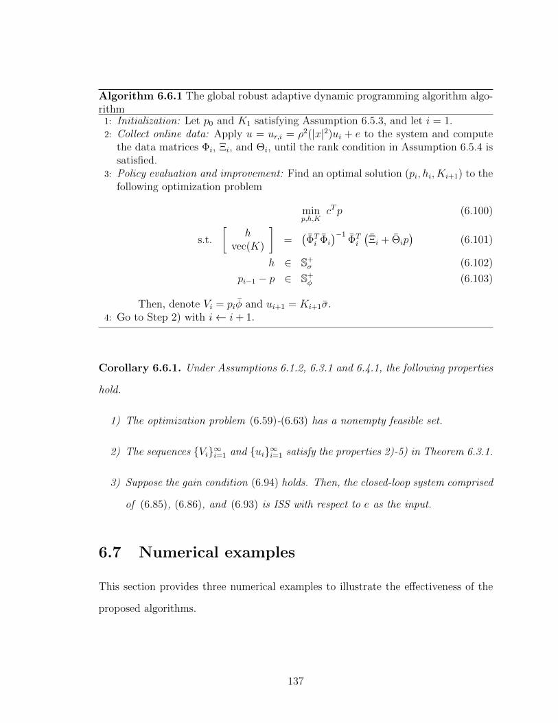
Algorithm 6.6.1 The global robust adaptive dynamic programming algorithm algo-rithm1: Initialization: Let p0 and K1 satisfying Assumption 6.5.3, and let i = 1.2: Collect online data: Apply u = ur,i = ρ2(|x|2)ui + e to the system and compute
the data matrices Φi, Ξi, and Θi, until the rank condition in Assumption 6.5.4 issatisfied.
3: Policy evaluation and improvement: Find an optimal solution (pi, hi, Ki+1) to thefollowing optimization problem
minp,h,K
cTp (6.100)
s.t.
[h
vec(K)
]=
(ΦTi Φi
)−1ΦTi
(Ξi + Θip
)(6.101)
h ∈ S+σ (6.102)
pi−1 − p ∈ S+φ (6.103)
Then, denote Vi = piφ and ui+1 = Ki+1σ.4: Go to Step 2) with i← i+ 1.
Corollary 6.6.1. Under Assumptions 6.1.2, 6.3.1 and 6.4.1, the following properties
hold.
1) The optimization problem (6.59)-(6.63) has a nonempty feasible set.
2) The sequences Vi∞i=1 and ui∞i=1 satisfy the properties 2)-5) in Theorem 6.3.1.
3) Suppose the gain condition (6.94) holds. Then, the closed-loop system comprised
of (6.85), (6.86), and (6.93) is ISS with respect to e as the input.
6.7 Numerical examples
This section provides three numerical examples to illustrate the effectiveness of the
proposed algorithms.
137
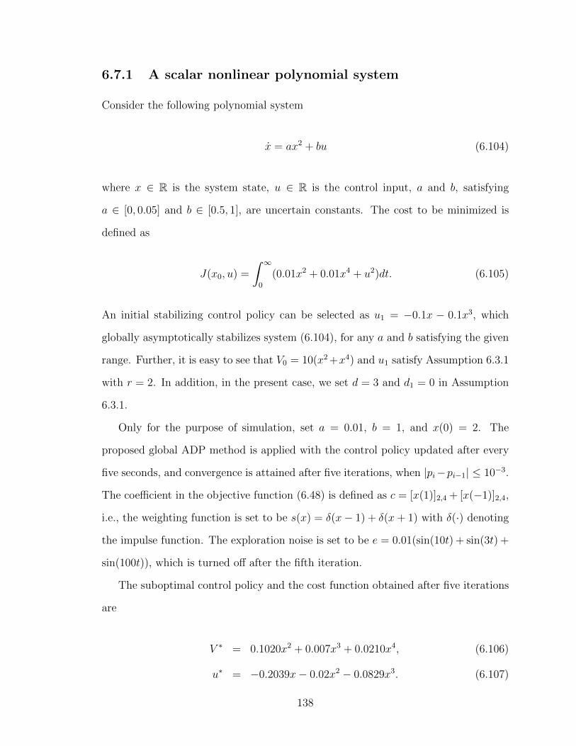
6.7.1 A scalar nonlinear polynomial system
Consider the following polynomial system
x = ax2 + bu (6.104)
where x ∈ R is the system state, u ∈ R is the control input, a and b, satisfying
a ∈ [0, 0.05] and b ∈ [0.5, 1], are uncertain constants. The cost to be minimized is
defined as
J(x0, u) =
∫ ∞
0
(0.01x2 + 0.01x4 + u2)dt. (6.105)
An initial stabilizing control policy can be selected as u1 = −0.1x − 0.1x3, which
globally asymptotically stabilizes system (6.104), for any a and b satisfying the given
range. Further, it is easy to see that V0 = 10(x2 +x4) and u1 satisfy Assumption 6.3.1
with r = 2. In addition, in the present case, we set d = 3 and d1 = 0 in Assumption
6.3.1.
Only for the purpose of simulation, set a = 0.01, b = 1, and x(0) = 2. The
proposed global ADP method is applied with the control policy updated after every
five seconds, and convergence is attained after five iterations, when |pi−pi−1| ≤ 10−3.
The coefficient in the objective function (6.48) is defined as c = [x(1)]2,4 + [x(−1)]2,4,
i.e., the weighting function is set to be s(x) = δ(x− 1) + δ(x+ 1) with δ(·) denoting
the impulse function. The exploration noise is set to be e = 0.01(sin(10t) + sin(3t) +
sin(100t)), which is turned off after the fifth iteration.
The suboptimal control policy and the cost function obtained after five iterations
are
V ∗ = 0.1020x2 + 0.007x3 + 0.0210x4, (6.106)
u∗ = −0.2039x− 0.02x2 − 0.0829x3. (6.107)
138
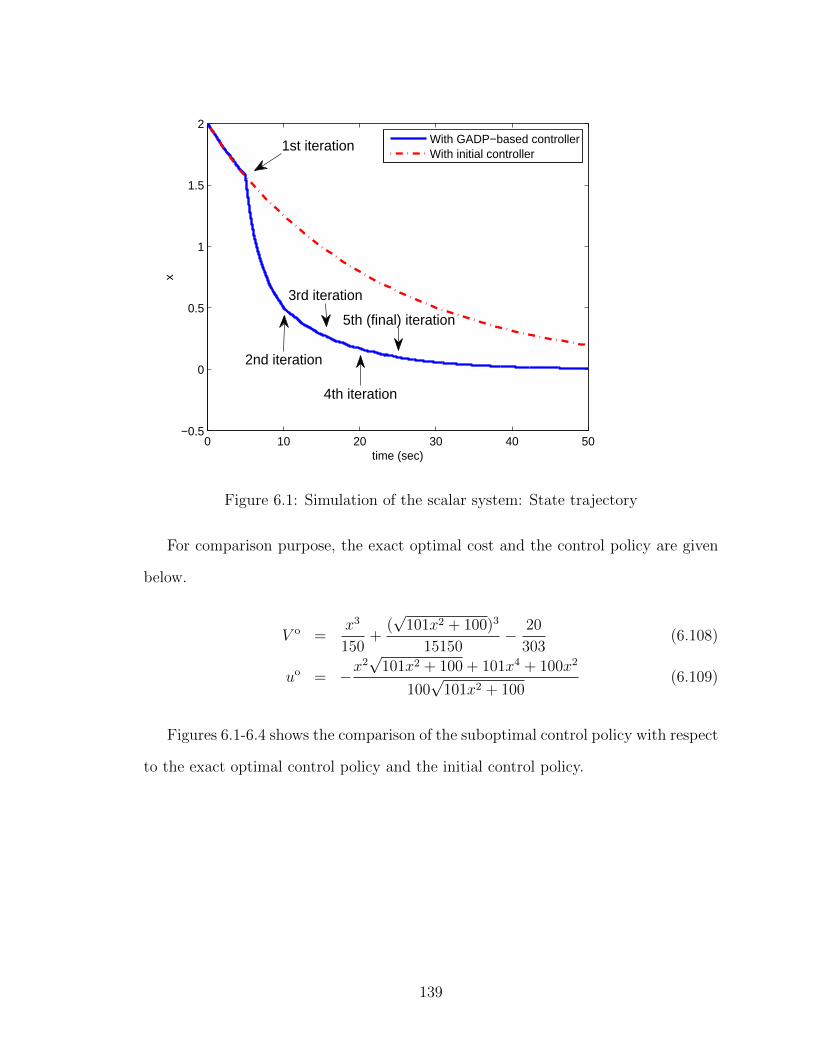
0 10 20 30 40 50−0.5
0
0.5
1
1.5
2
time (sec)
x
With GADP−based controllerWith initial controller
1st iteration
3rd iteration
2nd iteration
5th (final) iteration
4th iteration
Figure 6.1: Simulation of the scalar system: State trajectory
For comparison purpose, the exact optimal cost and the control policy are given
below.
V o =x3
150+
(√
101x2 + 100)3
15150− 20
303(6.108)
uo = −x2√
101x2 + 100 + 101x4 + 100x2
100√
101x2 + 100(6.109)
Figures 6.1-6.4 shows the comparison of the suboptimal control policy with respect
to the exact optimal control policy and the initial control policy.
139
0 10 20 30 40 50−0.5
0
0.5
1
1.5
2
time (sec)
u
1st iteration3rd iteration
2nd iteration
4th iteration 5th (final) iteration
Figure 6.2: Simulation of the scalar system: Control input
−2.5 −2 −1.5 −1 −0.5 0 0.5 1 1.5 2 2.50
0.5
1
1.5
2
2.5
3
3.5
x
V1 : Initial cost
V5: Improved cost
Vo: Optimal cost
Figure 6.3: Simulation of the scalar system: Cost functions
140
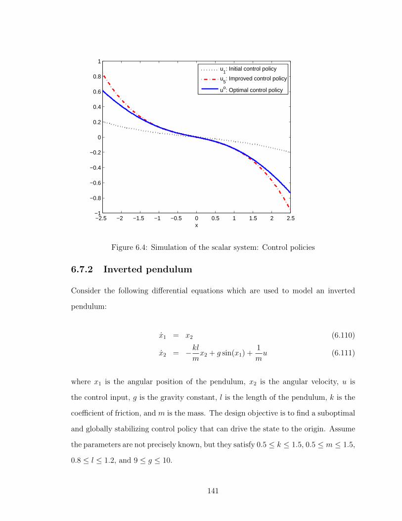
−2.5 −2 −1.5 −1 −0.5 0 0.5 1 1.5 2 2.5−1
−0.8
−0.6
−0.4
−0.2
0
0.2
0.4
0.6
0.8
1
x
u
1: Initial control policy
u5: Improved control policy
uo: Optimal control policy
Figure 6.4: Simulation of the scalar system: Control policies
6.7.2 Inverted pendulum
Consider the following differential equations which are used to model an inverted
pendulum:
x1 = x2 (6.110)
x2 = −klmx2 + g sin(x1) +
1
mu (6.111)
where x1 is the angular position of the pendulum, x2 is the angular velocity, u is
the control input, g is the gravity constant, l is the length of the pendulum, k is the
coefficient of friction, and m is the mass. The design objective is to find a suboptimal
and globally stabilizing control policy that can drive the state to the origin. Assume
the parameters are not precisely known, but they satisfy 0.5 ≤ k ≤ 1.5, 0.5 ≤ m ≤ 1.5,
0.8 ≤ l ≤ 1.2, and 9 ≤ g ≤ 10.
141

Notice that we can select φ = [x1, x2]T and σ = [x1, x2, sinx1]T . The cost is
selected as J(x0, u) =∫∞
0(10x2
1 + 10x2 + u2)dt.
Further, set φ = [x21, x1x2, x2
2]T and σ = [x21, x2
2, x1 sinx1, sin2 x1, x2 sinx1,
x1x2]T . Then, based on the range of the system parameters, a pair (V0, u1) sat-
isfying Assumption 6.5.3 can be obtained as u1 = −10x21 − x2 − 15 sinx1, and
V0 = 320.1297x21 + 46.3648x1x2 + 22.6132x2
2. The coefficient vector c is defined as
c = φ(1,−1) + φ(1, 1).
The initial condition for the system is set to be x1(0) = −1.5 and x2(0) = 1.
The control policy is updated after 0.5 seconds, until convergence is attained after 4
iterations. The exploration noise we use is the sum of sinusoidal waves with different
frequencies, and it is terminated once the convergence is attained.
The resultant control policy and the cost function are u∗ = −20.9844x1−7.5807x2
and V ∗ = 86.0463x21 + 41.9688x1x2 + 7.5807x2
2. Simulation results are provided in
Figures 6.5-6.6. It can be seen that the system performance is significantly improved
under the proposed ADP scheme.
6.7.3 Jet engine surge and stall dynamics
Consider the following system, which is inspired by the jet engine surge and stall
dynamics in [94, 119]
r = −σr2 − σr(2φ+ φ2
)(6.112)
φ = −aφ2 − bφ3 − (u+ 3rφ+ 3r) (6.113)
where r > 0 is the normalized rotating stall amplitude, φ is the deviation of the scaled
annulus-averaged flow, u is the deviation of the plenum pressure rise and is treated
as the control input, σ ∈ [0.2, 0.5], a ∈ [1.2, 1.6], b ∈ [0.3, 0.7] are uncertain constants.
In this example, we assume the variable r is not available for real-time feedback
142
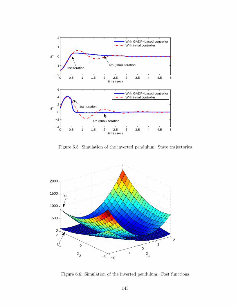
0 0.5 1 1.5 2 2.5 3 3.5 4 4.5 5−2
−1
0
1
2
x 1
time (sec)
0 0.5 1 1.5 2 2.5 3 3.5 4 4.5 5−4
−2
0
2
4
6
time (sec)
x 2
With GADP−based controllerWith initial controller
With GADP−based controllerWith initial controller
4th (final) iteration1st iteration
1st iteration
4th (final) iteration
Figure 6.5: Simulation of the inverted pendulum: State trajectories
−2−1
01
2
−5
0
50
500
1000
1500
2000
x1
x2
V4
V1
Figure 6.6: Simulation of the inverted pendulum: Cost functions
143
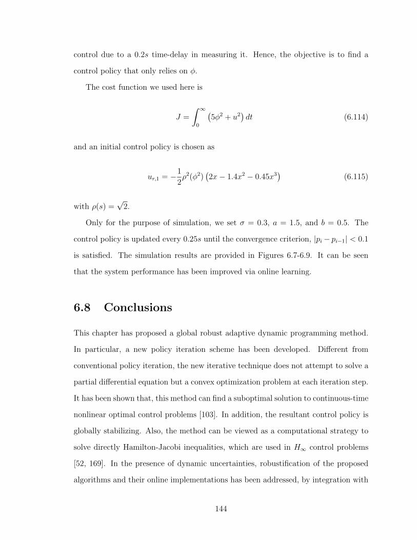
control due to a 0.2s time-delay in measuring it. Hence, the objective is to find a
control policy that only relies on φ.
The cost function we used here is
J =
∫ ∞
0
(5φ2 + u2
)dt (6.114)
and an initial control policy is chosen as
ur,1 = −1
2ρ2(φ2)
(2x− 1.4x2 − 0.45x3
)(6.115)
with ρ(s) =√
2.
Only for the purpose of simulation, we set σ = 0.3, a = 1.5, and b = 0.5. The
control policy is updated every 0.25s until the convergence criterion, |pi− pi−1| < 0.1
is satisfied. The simulation results are provided in Figures 6.7-6.9. It can be seen
that the system performance has been improved via online learning.
6.8 Conclusions
This chapter has proposed a global robust adaptive dynamic programming method.
In particular, a new policy iteration scheme has been developed. Different from
conventional policy iteration, the new iterative technique does not attempt to solve a
partial differential equation but a convex optimization problem at each iteration step.
It has been shown that, this method can find a suboptimal solution to continuous-time
nonlinear optimal control problems [103]. In addition, the resultant control policy is
globally stabilizing. Also, the method can be viewed as a computational strategy to
solve directly Hamilton-Jacobi inequalities, which are used in H∞ control problems
[52, 169]. In the presence of dynamic uncertainties, robustification of the proposed
algorithms and their online implementations has been addressed, by integration with
144
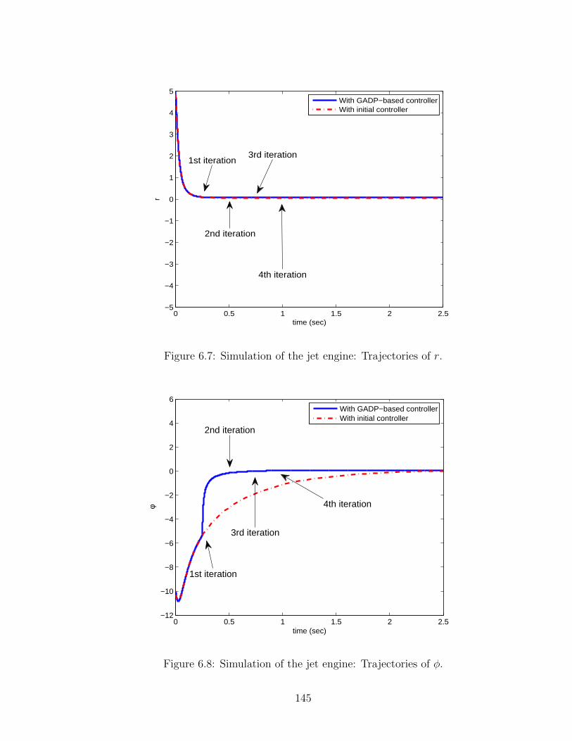
0 0.5 1 1.5 2 2.5−5
−4
−3
−2
−1
0
1
2
3
4
5
time (sec)
r
With GADP−based controllerWith initial controller
1st iteration
2nd iteration
3rd iteration
4th iteration
Figure 6.7: Simulation of the jet engine: Trajectories of r.
0 0.5 1 1.5 2 2.5−12
−10
−8
−6
−4
−2
0
2
4
6
time (sec)
φ
With GADP−based controllerWith initial controller
2nd iteration
1st iteration
4th iteration
3rd iteration
Figure 6.8: Simulation of the jet engine: Trajectories of φ.
145

−2.5 −2 −1.5 −1 −0.5 0 0.5 1 1.5 2 2.5−10
0
10
20
30
40
50
60
70
80
φ
V
1 : Initial cost
V5: Improved cost
Vo: Optimal cost
Figure 6.9: Simulation of the jet engine: Value functions.
the ISS property [149, 151] and the nonlinear small-gain theorem [83, 81].
When the system parameters are unknown, conventional ADP methods utilize
neural networks to approximate online the optimal solution, and a large number of
basis functions are required to assure high approximation accuracy on some compact
sets. Thus, neural-network-based ADP schemes may result in slow convergence and
loss of global asymptotic stability for the closed-loop system. Here, the proposed
GRADP method has overcome the two above-mentioned shortcomings, and it yields
computational benefits.
146

Chapter 7
RADP as a theory of sensorimotor
control
Many tasks that humans perform in our daily lives involve different sources of uncer-
tainties. However, it is interesting and surprising to notice how the central nervous
system can coordinate gracefully our movements to deal with these uncertainties. For
example, one may be clumsy in moving an object with uncertain mass and unknown
friction at the first time, but after several trials, the movements will gradually become
smooth. Although extensive research by many authors has been made, the underlying
computational mechanisms in sensorimotor control require further investigations.
From different aspects, many theories have been proposed to explain the computa-
tional nature of sensorimotor control; see the review article [43]. One widely accepted
view is that the central nervous system (CNS) prefers trajectories produced by min-
imizing some cost function. This perspective has inspired quite a few optimization-
based models for motor control (see [33, 40, 50, 55, 77, 131, 140, 163, 162, 165], and
references therein). These models can explain many characteristics of motor control,
such as approximately straight movement trajectories and the bell-shaped velocity
curves reported by [120]. However, these models assume the CNS knows and uses the
147
dynamics of both the motor system and the interactive environment. Consequently,
an indirect control scheme is assumed. Namely, the CNS first identifies all the system
dynamics, and then finds the optimal control policies based on the identified infor-
mation. This identification-based idea has also been used to study motor adaptation
under external perturbations [9, 13, 31, 92, 142, 195]. Nevertheless, this viewpoint
is difficult to be justified theoretically and has not been convincingly validated by
experiments. Using self-generated perturbation, [59] reported that disturbance may
not be identified by the CNS, and the control policy may not necessarily be optimal in
the presence of uncertainties. Indeed, when uncertainties, especially dynamic uncer-
tainties, occur, it becomes difficult to maintain not only optimality, but also stability.
Since the optimization-based model may not be suitable to study the behavior and
stability of motor systems, developing a new theoretical modeling framework is not
only necessary but also of great importance.
The primary objective of this chapter is to study sensorimotor control with static
and dynamic uncertainties under the framework of RADP [68, 69, 72, 73, 79]. In this
chapter, the linear version of RADP is extended for stochastic systems by taking into
account signal-dependent noise [50], and the proposed method is applied to study the
sensorimotor control problem with both static and dynamic uncertainties.
There are two main advantages of the proposed modeling strategy. First of all, as a
non-model-based approach, RADP shares some essential features with reinforcement
learning (RL) [155], which is originally inspired by learning mechanisms observed in
biological systems. RL concerns how an agent should modify its actions to interact
with the unknown environment and to achieve a long-term goal. In addition, certain
brain areas that can realize the steps of RL have been discussed by [36]. Like in many
other ADP-based methods, the proposed RADP theory solves the Bellman equation
[8] iteratively using real-time sensory information and can avoid the so-called “curse
of dimensionality” in conventional dynamic programming. Also, rigorous convergence
148
analysis can be performed. Second, instead of identifying the dynamics of the overall
dynamic system, we decompose the system into an interconnection of a simplified
model (nominal system) with measurable state variables and the dynamic uncertainty
(or, unmodeled dynamics) with unmeasurable state variables and unknown system
order (see Figure 7.1). Then, we design the robust optimal control policy for the
overall system using partial-state feedback. In this way, we can preserve optimality
for the nominal reduced model as well as guarantee robust stability for the overall
system. Compared with identification-based models, this modeling strategy is more
realistic for sensorimotor systems for at least two reasons. First, identifying the exact
model of both the motor system and the uncertain environment is not an easy task.
Second, it is time-consuming and would yield slow response if the sensorimotor system
first estimates all system variables before taking actions.
Detailed learning algorithms are presented in this chapter, and numerical studies
are also provided. Interestingly, our computational results match well with exper-
iments reported from the past literature [22, 41, 142]. The proposed theory also
provides a unified theoretical framework that connects optimality and robustness. In
addition, it links the stiffness geometry to the selection of the weighting matrices in
the cost function. Therefore, we argue that the CNS may use RADP-like learning s-
trategy to coordinate movements and to achieve successful adaptation in the presence
of static and/or dynamic uncertainties. In the absence of the dynamic uncertainties,
the learning strategy reduces to an ADP-like mechanism.
149
7.1 ADP for continuous-time stochastic systems
7.1.1 Problem formulation
To study sensorimotor control, we consider the following system governed by stochas-
tic differential equations:
dx = Axdt+Budt+BΣqi=1Ciudηi (7.1)
where A ∈ Rn×n and B ∈ Rn×m are constant matrices describing the system dynamics
with the pair (A,B) assumed to be stabilizable (i.e., there exists some constant matrix
K0 ∈ Rm×n such that A−BK0 is a Hurwitz matrix in the sense that all its eigenvalues
are in the open left-half plane), u ∈ Rm is the control signal, ηi are independent scalar
Brownian motions and Ci ∈ Rm×m are constant matrices, for i = 1, 2, · · · , q.
The control objective is to determine a linear control policy
u = −Kx (7.2)
which minimizes the following cost function
J =
∫ ∞
0
(xTQx+ uTRu)dt (7.3)
for the nominal system of (7.1) (i.e., system (7.1) with ηi = 0, ∀i = 1, 2, · · · ,m),
where Q = QT ≥ 0, R = RT > 0, with (A,Q1/2) observable. By observability, we
mean that the solution x(t) of the system dx = Axdt is identically zero when the
output y = Q1/2x is identically zero [99].
According to linear optimal control theory [99], when both A and B are accurately
known, solution to this problem can be found by solving the following well-known
150
algebraic Riccati equation (ARE)
ATP + PA+Q− PBR−1BTP = 0. (7.4)
By the assumptions mentioned above, (7.4) has a unique symmetric positive def-
inite solution P ∗ ∈ Rn×n. The optimal feedback gain matrix K∗ in (7.2) can thus be
determined by
K∗ = R−1BTP ∗. (7.5)
In the presence of the signal-dependent noise ηi, the closed-loop system is mean-
square stable [90], if
0 > (A−BK∗)⊗ In + In ⊗ (A−BK∗)
+Σqi=1 (BCiK
∗ ⊗BCiK∗) . (7.6)
If the constant matrices Ci, i = 1, 2, · · · , q, are so small that (7.6) holds, the
control policy u = −K∗x is called robust optimal, i.e., it is optimal in the absence of
the noise ηi, and is stabilizing in the presence of ηi.
7.1.2 Policy iteration
To solve (7.4) which is nonlinear in P , the policy iteration algorithm from reinforce-
ment learning can be applied [91], and in [91], it has been proved that the sequences
Pk and Kk iteratively determined from policy iteration (7.7) and (7.8) have the
following properties:
1) A−BKk is Hurwitz,
2) P ∗ ≤ Pk+1 ≤ Pk, and
151
3) limk→∞
Kk = K∗, limk→∞
Pk = P ∗.
Algorithm 7.1.1 Policy iteration with control-dependent noise
1: Find an initial stabilizing feedback gain matrix K0, such that A−BK0 is Hurwitz.2: Solve Pk from
0 = (A−BKk)TPk + Pk(A−BKk) +Q+KT
k RKk (7.7)
3: Improve the control policy by
Kk+1 = R−1BTPk (7.8)
4: Go to Step 2) and solve for Pk+1 with Kk replaced by Kk+1.
7.1.3 ADP for linear stochastic systems with signal-dependent
noise
The policy iteration algorithm relies on the perfect knowledge of the system dynamics,
because the system matrices A and B are involved in the equations (7.7) and (7.8).
In [68], it has been shown that in the deterministic case, when A and B are unknown,
equivalent iterations can be achieved using online measurements. Here we extend
the methodology by [68] to deal with stochastic linear systems with signal-dependent
noise, and to find online the optimal control policy without assuming the a priori
knowledge of A and B.
To begin with, let us rewrite the original system (7.1) as
dx = (A−BKk)xdt+B(dw +Kkxdt) (7.9)
where
dw = udt+ Σqi=1Ciudηi (7.10)
represents the combined signal received by the motor plant from the input channel.
152
Now, let us define Ak = A−BKk, Qk = Q+KTk RKk, and Mk = BTPkB. Then,
by Ito’s lemma [62], along the solutions of (7.53), it follows that
d(xTPkx)
= dxTPkx+ xTPkdx+ dxTPkdx
= xT (ATkPk + PkAk)xdt+ 2(Kkxdt+ dw)TBTPkx
+dwTBTPkBdw
= −xTQkxdt+ 2(Kkxdt+ dw)TBTPkx+ dwTMkdw (7.11)
Notice that dwTMkdw 6= 0 because
dwTMkdw
= (udt+ Σqi=1Ciudηi)
TMk(udt+ Σqi=1Ciudηi)
= uTMku(dt)2 + Σqi=1u
TCTi MkCiu(dηi)
2
+Σ1≤i 6=j≤quTCT
i MkCiudηidηj
= Σqi=1u
TCTi MkCiudt
Next, integrating both sides of (7.55) from t to t+ δt, we obtain
x(t+ δt)TPkx(t+ δt)− x(t)TPkx(t)
= −∫ t+δt
t
(xTQx+ uTkRuk
)dt+
∫ t+δt
t
dwTMkdw (7.12)
+2
∫ t+δt
t
(Kkx+ dw)TRKk+1x
where uk = −Kkx.
Notice that (7.59) plays an important role in separating accurately the system
dynamics from the iterative process. As a result, the requirement of the system
matrices in (7.7) and (7.8) can now be replaced by the state and input information
153
measured in real-time.
We now show that given a matrix Kk such that A − BKk is Hurwitz, a pair of
matrices (Pk, Kk+1), with Pk = P Tk > 0, satisfying (7.7) and (7.8) can be uniquely
determined without knowing A or B . To this end, recall that we have defined the
following two operators:
P ∈ Rn×n → P ∈ R12n(n+1)
x ∈ Rn → x ∈ R12n(n+1)
where
P = [p11, 2p12, · · · , 2p1n, p22, 2p23, · · · , 2pn−1,n, pnn]T ,
x = [x21, x1x2, · · · , x1xn, x
22, x2x3, · · · , xn−1xn, x
2n]T .
Therefore, by Kronecker product representation [56], we have
(Kkxdt+ dw)TRKk+1x = [x⊗R(Kkxdt+ dw)]T vec(Kk+1).
Further, for a sufficiently large positive integer lk > 0, we define matrices δx,k ∈
Rlk× 12n(n+1), Iq,k ∈ Rlk , Ixv,k ∈ Rlk×mn, and Iu,k ∈ Rlk× 1
2m(m+1), such that
δx,k =
xT (t1,k)− xT (t0,k)
xT (t2,k)− xT (t1,k)
...
xT (tlk,k)− xT (tlk−1,k)
,
154
Iq,k =
∫ t1,kt0,k
(xTQx+ uTkRuk
)dt
∫ t2,kt1,k
(xTQx+ uTkRuk
)dt
· · ·∫ tlk,ktlk−1,k
(xTQx+ uTkRuk
)dt
,
Ixv,k =
∫ t1,kt0,k
xT ⊗ (Kkxdt+ dw)TR∫ t2,kt1,k
xT ⊗ (Kkxdt+ dw)TR
...∫ tlk,ktlk−1,k
xT ⊗ (Kkxdt+ dw)TR
,
Iu,k =
∫ t1,kt0,k
wTdτ∫ t2,kt1,k
wTdτ
· · ·∫ tlk,ktlk−1,k
wTdτ
where 0 ≤ tlk−1,k−1 ≤ t0,k < t1,k < · · · < tlk,k < t0,k+1.
Therefore, (7.59) implies the following compact form of linear equations
Θk
Pk
Mk
vec (Kk+1)
= −Iq,k (7.13)
where Θk ∈ Rlk×[ 12n(n+1)+mn] is defined as:
Θk = [δx,k,−Iu,k,−2Ixv,k] ,
To guarantee the existence and uniqueness of solution to (7.62), we assume Θk has
155
full column rank for all k ∈ Z+. As a result, (7.62) can be directly solved as follows:
Pk
Mk
vec (Kk+1)
= −(ΘTkΘk)
−1ΘTk Iq,k. (7.14)
It is worth noticing that when the sensory noise is taken into account, numerical
errors may occur when computing the matrices Iq,k, Ixv,k, and Iu,k. Consequently, the
solution of (7.14) can be viewed as the least squares solution of (7.62). Alternatively,
an approximation of the unique solution of (7.62) can be obtained using a recursive
least-squares method [111].
7.1.4 The ADP algorithm
Now, we are ready to give the following ADP algorithm for practical online imple-
mentation.
Algorithm 7.1.2 Adaptive dynamic programming algorithm
1: Find an initial stabilizing control policy u0 = −K0x, and set k = 0.2: Apply uk = −Kkx as the control input on the time interval [t0,k, tlk,k]. Computeδx,k, Iq,k, Ixv,k, and Iu,k.
3: Solve Pk, Mk, and Kk+1 from (7.14).4: Let k ← k + 1, and go to Step 2.
Compared with most of the existing models for motor adaptation, the proposed
ADP algorithm can be used to study both the online learning during one single trial
and the learning among different trials. In the latter case, the interval [t0,k, tlk,k]
should be taken from the time duration of a single trial.
7.1.5 Convergence analysis
The convergence property of the proposed algorithm can be summarized in the fol-
lowing Theorem.
156
Theorem 7.1.1. Suppose Θk has full column rank for all k ∈ Z+ and A − BK0 is
Hurwitz. Then, the sequences Kk, Pk, and Mk obtained from (7.14) satisfy
limk→∞
Pk = P ∗, limk→∞
Kk = K∗, and limk→∞
Mk = BTP ∗B.
Proof. Given a stabilizing feedback gain matrix Kk, if Pk = P Tk is the solution of
(7.7), Kk+1 and Mk are uniquely determined by Kk+1 = R−1BTPk and Mk = BTPkB,
respectively. By (7.59), we know that Pk, Kk+1, and Mk satisfy (7.14).
On the other hand, let P = P T ∈ Rn×n, M ∈ Rm×m, and K ∈ Rm×n, such that
Θk
P
M
vec(K)
= Ξk. (7.15)
Then, we immediately have P = Pk, M = Mk , and vec(K) = vec(Kk+1). Since Θk
has full column rank, P = P T , M = MT , and K are unique. In addition, by the
definitions of P , M , and vec(K), Pk = P , Mk = M and Kk+1 = K are uniquely
determined. Therefore, the policy iteration (7.14) is equivalent to (7.7) and (7.8). By
[91], the convergence is thus proved.
7.2 RADP for continuous-time stochastic systems
7.2.1 Problem formulation
In this paper, we generalize the commonly used linear models for sensorimotor control
([50, 40, 63, 163]) by taking into account the dynamic uncertainty, or unmodeled
157
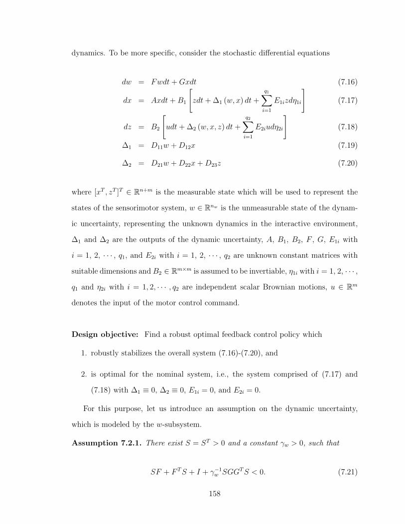
dynamics. To be more specific, consider the stochastic differential equations
dw = Fwdt+Gxdt (7.16)
dx = Axdt+B1
[zdt+ ∆1 (w, x) dt+
q1∑
i=1
E1izdη1i
](7.17)
dz = B2
[udt+ ∆2 (w, x, z) dt+
q2∑
i=1
E2iudη2i
](7.18)
∆1 = D11w +D12x (7.19)
∆2 = D21w +D22x+D23z (7.20)
where [xT , zT ]T ∈ Rn+m is the measurable state which will be used to represent the
states of the sensorimotor system, w ∈ Rnw is the unmeasurable state of the dynam-
ic uncertainty, representing the unknown dynamics in the interactive environment,
∆1 and ∆2 are the outputs of the dynamic uncertainty, A, B1, B2, F , G, E1i with
i = 1, 2, · · · , q1, and E2i with i = 1, 2, · · · , q2 are unknown constant matrices with
suitable dimensions andB2 ∈ Rm×m is assumed to be invertiable, η1i with i = 1, 2, · · · ,
q1 and η2i with i = 1, 2, · · · , q2 are independent scalar Brownian motions, u ∈ Rm
denotes the input of the motor control command.
Design objective: Find a robust optimal feedback control policy which
1. robustly stabilizes the overall system (7.16)-(7.20), and
2. is optimal for the nominal system, i.e., the system comprised of (7.17) and
(7.18) with ∆1 ≡ 0, ∆2 ≡ 0, E1i = 0, and E2i = 0.
For this purpose, let us introduce an assumption on the dynamic uncertainty,
which is modeled by the w-subsystem.
Assumption 7.2.1. There exist S = ST > 0 and a constant γw > 0, such that
SF + F TS + I + γ−1w SGGTS < 0. (7.21)
158
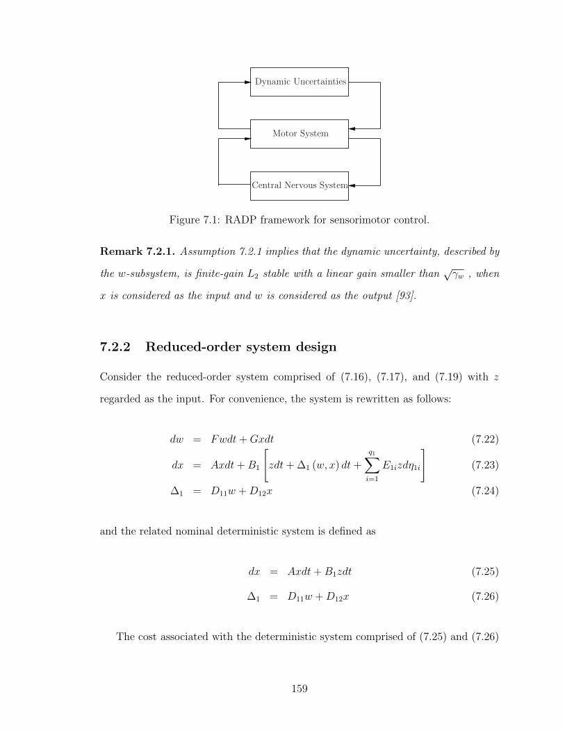
Dynamic Uncertainties
Motor System
Central Nervous System
Figure 7.1: RADP framework for sensorimotor control.
Remark 7.2.1. Assumption 7.2.1 implies that the dynamic uncertainty, described by
the w-subsystem, is finite-gain L2 stable with a linear gain smaller than√γw , when
x is considered as the input and w is considered as the output [93].
7.2.2 Reduced-order system design
Consider the reduced-order system comprised of (7.16), (7.17), and (7.19) with z
regarded as the input. For convenience, the system is rewritten as follows:
dw = Fwdt+Gxdt (7.22)
dx = Axdt+B1
[zdt+ ∆1 (w, x) dt+
q1∑
i=1
E1izdη1i
](7.23)
∆1 = D11w +D12x (7.24)
and the related nominal deterministic system is defined as
dx = Axdt+B1zdt (7.25)
∆1 = D11w +D12x (7.26)
The cost associated with the deterministic system comprised of (7.25) and (7.26)
159
is selected to be
J1 =
∫ ∞
0
(xTQ1x+ zTR1z
)dt (7.27)
where Q1 = QT1 ≥ 0, R1 = RT
1 > 0, and the pair (A,Q1/21 ) is observable.
By linear optimal control theory [99], the optimal control policy takes the following
form
z = −R−11 BT
1 P1x (7.28)
where P1 = P T1 > 0 is the solution of the following algebraic Riccati Equation (ARE):
ATP1 + P1A+Q1 − P1B1R−11 BT
1 P1 = 0. (7.29)
The following concept on mean-square stability [194] will be used in the remainder
of the paper.
Definition 7.2.1. Consider the system
dx = Axdt+
q∑
i=1
Bixdηi (7.30)
where ηi with i = 1, 2, · · · , q are standard scalar Brownian motions. Then, the system
is said to be stable in the mean-square sense if
limt→∞
E[x(t)x(t)T
]= 0. (7.31)
Now, the following theorem gives stability criteria of the closed-loop system com-
prised of (7.22), (7.23), (7.24), and (7.28).
Theorem 7.2.1. The closed-loop system comprised of (7.22), (7.23), (7.24), and
160
(7.28) is mean-square stable if
1. the weighting matrices Q1 and R1 are selected such that
Q1 > (κ12 + κ11γw) In and R1 < Im (7.32)
where κ11 = 2|D11|2 and κ12 = 2|D12|2.
2. the constant matrices E1i with i = 1, 2, · · · , q1 satisfy
q1∑
i=1
ET1iB
T1 P1B1E1i ≤ R1(Im −R1) (7.33)
Proof. First, we define L(·) as the infinitesimal generator [98]. Then, along the tra-
jectories of the x-subsystem, (7.23), we have
L(xTP1x) = −xT(Q1 + P1B1R
−1BT1 P1
)x+ 2xTP1B1∆1
+xTP1B1R−11
q1∑
i=1
ET1iB
T1 P1B1E1iR
−11 BT
1 P1x
= −xTQ1x− |∆1 −BT1 P
T1 x|2dt+ |∆1|2
−xTP1B1R−11
[R1 −R2
1 −q1∑
i=1
ET1iB
T1 P1B1E1i
]
×R−11 BT
1 P1x
≤ −xTQ1x+ |∆1|2
On the other hand, under Assumption 7.2.1, along the solutions of the w-subsystem
(7.22), we have
L(wTSw
)= wT (SF + F TS)w + wTSGx+ xTGTSw
< −|w|2 − γw−1wTSGGTSw + wTSGx+ xTGTSw
< −|w|2 + γw|x|2 (∀w 6= 0)
161
By definition, we know that
|∆1|2 = |D11w +D12x|2
≤ 2|D11|2|w|2 + 2|D12|2|x|2
≤ κ11|w|2 + κ12|x|2
Therefore, for all (x,w) 6= 0, the following holds
L(xTP1x+ κ11wTSw)
< −γx|x|2 + |∆1|2 − κ11|w|2 + κ11γw|x|2
< −γx|x|2 + κ11|w|2 + 2xTDT12D12x− κ11|w|2 + κ11γw|x|2
< −xT (Q1 − κ12In − κ11γwIn)x
< 0
Notice that V (w, x) = xTP1x+κ11wTSw can be regarded as a stochastic Lyapunov
function [98], and the proof is thus complete.
7.2.3 Optimal control design for the full system
Now we proceed ahead to study the full system. Define the transformation
ξ = z +K1x (7.34)
162
where K1 = R−11 BT
1 P1. Then, we have
dξ = dz +K1dx
= B2
[udt+ ∆2dt+
q2∑
i=1
E2iudη2i
]
+K1(Acxdt+B1∆1dt+B1ξdt+B1
q1∑
i=1
E1izdη1i)
= K1Acxdt+B2udt+B2∆2dt+K1B1ξdt
+
q2∑
i=1
B2E2iudη2i +K1
q1∑
i=1
B1E1i (ξ −K1x) dη1i
where ∆2 = B−12 K1B1∆1 + ∆2 and Ac = A−B1K1.
Consequently, the system (7.16)-(7.20) is converted to
dw = Fwdt+Gxdt (7.35)
dx = Acxdt+B1
[ξdt+ ∆1dt+
q1∑
i=1
E1i (ξ −K1x) dη1i
](7.36)
dξ = K1Acxdt+B2udt+B2∆2dt+K1B1ξdt
+
q2∑
i=1
B2E2iudη2i +K1
q1∑
i=1
B1E1i (ξ −K1x) dη1i (7.37)
Now, let us consider the control policy
u = −R−12 BT
2 P2ξ = −R−12 BT
2 P2
(z +R−1
1 B1P1x)
(7.38)
where P2 = P T2 > 0 is the solution of the following equation
Q2 − P2B2R−12 BT
2 P2 = 0 (7.39)
with Q2 and R2 two positive definite and symmetric matrices.
Remark 7.2.2. Notice that (7.39) is an ARE associated with the following optimal
163

control problem
minu
J2 =
∫ ∞
0
(zTQ2z + uTR2u
)dt, (7.40)
s.t. z = B2u, (7.41)
where (7.41) is the nominal system of (7.18).
The stability criteria are given in the following theorem.
Theorem 7.2.2. The closed-loop system comprised of (7.35)-(7.37) and (7.38) is
mean-square stable if
1. the weighting matrices Q1 and R1 as defined in (7.29), and Q2 and R2 as defined
in (7.39) are selected such that R1 < Im, R2 < Im and
(κ12 + κ22 + γwκ11 + γwκ21) In − ATcKT1 P2 − P1B1
−P2K1Ac −BT1 P1 (κ23 + κ3) Im
<
Q1 0
0 Q2
(7.42)
2. the constant matrices E1i and E2i satisfy the following inequalities
q1∑
i=1
ET1iB
T1
(P1 +KT
1 P2K1
)B1E1i ≤
1
2R1 (Im −R1) (7.43)
q2∑
i=1
ET2iB
T2 P2B2E2i ≤ R2 (Im −R2) (7.44)
164
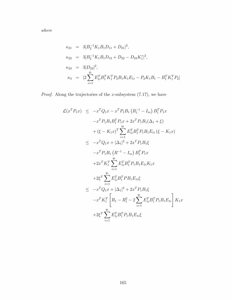
where
κ21 = 3|B−12 K1B1D11 +D21|2,
κ22 = 3|B−12 K1B1D12 +D22 −D23K
∗1 |2,
κ23 = 3|D23|2,
κ3 = |2q1∑
i=1
ET1iB
T1 K
T1 P2B1K1E1i − P2K1B1 −BT
1 KT1 P2|
Proof. Along the trajectories of the x-subsystem (7.17), we have
L(xTP1x) ≤ −xTQ1x− xTP1B1
(R−1
1 − Im)BT
1 P1x
−xTP1B1BT1 P1x+ 2xTP1B1(∆1 + ξ)
+ (ξ −K1x)Tq1∑
i=1
ET1iB
T1 P1B1E1i (ξ −K1x)
≤ −xTQ1x+ |∆1|2 + 2xTP1B1ξ
−xTP1B1
(R−1 − Im
)BT
1 P1x
+2xTKT1
q1∑
i=1
ET1iB
T1 P1B1E1iK1x
+2ξTq1∑
i=1
ET1iB
T1 PB1E1iξ
≤ −xTQ1x+ |∆1|2 + 2xTP1B1ξ
−xTKT1
[R1 −R2
1 − 2
q1∑
i=1
ET1iB
T1 P1B1E1i
]K1x
+2ξTq1∑
i=1
ET1iB
T1 P1B1E1iξ
165
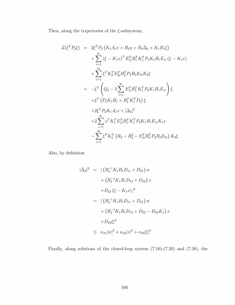
Then, along the trajectories of the ξ-subsystem,
L(ξTP2ξ) = 2ξTP2
(K1Acx+B2u+B2∆2 +K1B1ξ
)
+
q1∑
i=1
(ξ −K1x)T ET1iB
T1 K
T1 P2K1B1E1i (ξ −K1x)
+
q2∑
i=1
ξTKT2 E
T2iB
T2 P2B2E2iK2ξ
= −ξT(Q2 − 2
q1∑
i=1
ET1iB
T1 K
T1 P2K1B1E1i
)ξ
+ξT(P2K1B1 +BT
1 KT1 P2
)ξ
+2ξTP2K1Acx+ |∆2|2
+2
q1∑
i=1
xTKT1 E
T1iB
T1 K
T1 P2K1B1E1iK1x
−q2∑
i=1
ξTKT2
(R2 −R2
2 − ET2iB
T2 P2B2E2i
)K2ξ
Also, by definition
|∆2|2 = |(B−1
2 K1B1D11 +D21
)w
+(B−1
2 K1B1D12 +D22
)x
+D23 (ξ −K1x) |2
= |(B−1
2 K1B1D11 +D21
)w
+(B−1
2 K1B1D12 +D22 −D23K1
)x
+D23ξ|2
≤ κ21|w|2 + κ22|x|2 + κ23|ξ|2
Finally, along solutions of the closed-loop system (7.16)-(7.20) and (7.38), the
166

following holds for all [wT , xT , zT ] 6= 0
L[(κ11 + κ21)wTSw + xTP1x+ ξTP2ξ
])
≤ −
x
ξ
T Q1 − (κ12 + κ22 + κ11γ + κ21γ) In ATcK
T1 P2 + P1B1
P2K1Ac +BT1 P1 Q2 − (κ23 + κ3) Im
×
x
ξ
− xTKT
1
(R1 −R2
1
)K1x
+2xTKT1
q1∑
i=1
ET1iB
T1
(P1 +KT
1 P2K1
)B1E1iK1x
−ξTKT2
(R2 −R2
2 −q2∑
i=1
ET2iB
T2 P2B2E2i
)K2ξ
< 0
The proof is complete.
Remark 7.2.3. Consider the nominal system (7.35)-(7.37). In the absence of dy-
namic uncertainties (i.e., the w-subsystem is absent, ∆1 ≡ 0, ∆2 ≡ 0, E1i = 0 for
i = 1, 2, · · · , q1, and E2i = 0 for i = 1, 2, · · · , q2), the control policy (7.38) is optimal
in the sense that it minimizes the cost
J2 =
∫ ∞
0
x
ξ
T
Q2
x
ξ
+ uTR2u
dt (7.45)
where
Q2 =
Q1 +KT1 R1K1 ATcK
T1 P2 + P1B1
P2K1Ac +BT1 P1 Q2 − P2K1B1 −BT
1 KT1 P2
> 0
Notice that the design methodology is different from inverse optimal control [96].
Indeed, although the weighing matrix Q2 cannot be arbitrary specified, it can be indi-
167
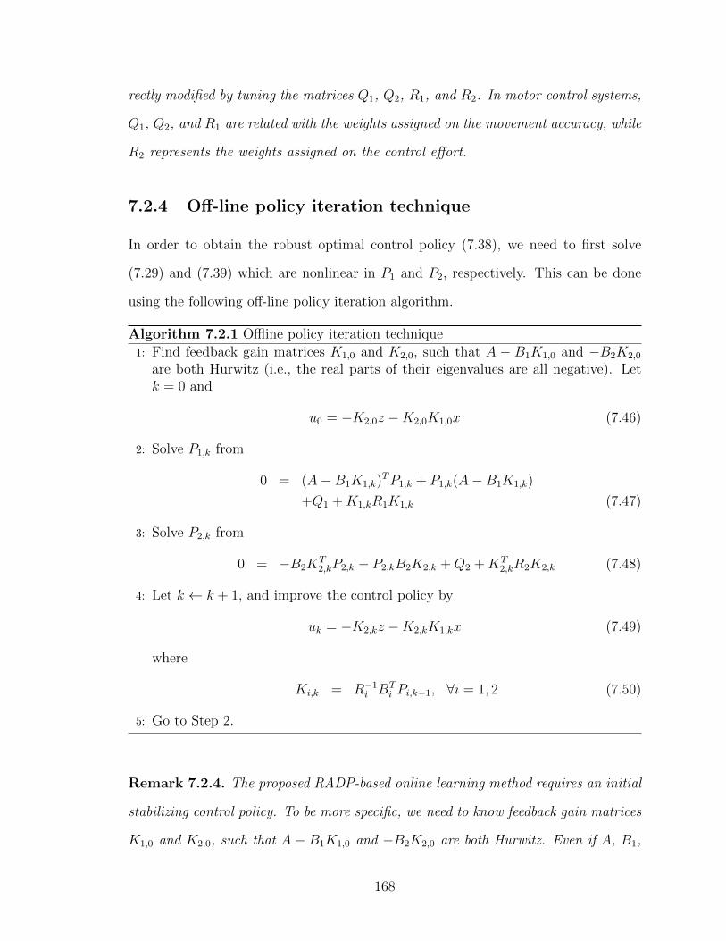
rectly modified by tuning the matrices Q1, Q2, R1, and R2. In motor control systems,
Q1, Q2, and R1 are related with the weights assigned on the movement accuracy, while
R2 represents the weights assigned on the control effort.
7.2.4 Off-line policy iteration technique
In order to obtain the robust optimal control policy (7.38), we need to first solve
(7.29) and (7.39) which are nonlinear in P1 and P2, respectively. This can be done
using the following off-line policy iteration algorithm.
Algorithm 7.2.1 Offline policy iteration technique
1: Find feedback gain matrices K1,0 and K2,0, such that A − B1K1,0 and −B2K2,0
are both Hurwitz (i.e., the real parts of their eigenvalues are all negative). Letk = 0 and
u0 = −K2,0z −K2,0K1,0x (7.46)
2: Solve P1,k from
0 = (A−B1K1,k)TP1,k + P1,k(A−B1K1,k)
+Q1 +K1,kR1K1,k (7.47)
3: Solve P2,k from
0 = −B2KT2,kP2,k − P2,kB2K2,k +Q2 +KT
2,kR2K2,k (7.48)
4: Let k ← k + 1, and improve the control policy by
uk = −K2,kz −K2,kK1,kx (7.49)
where
Ki,k = R−1i BT
i Pi,k−1, ∀i = 1, 2 (7.50)
5: Go to Step 2.
Remark 7.2.4. The proposed RADP-based online learning method requires an initial
stabilizing control policy. To be more specific, we need to know feedback gain matrices
K1,0 and K2,0, such that A− B1K1,0 and −B2K2,0 are both Hurwitz. Even if A, B1,
168
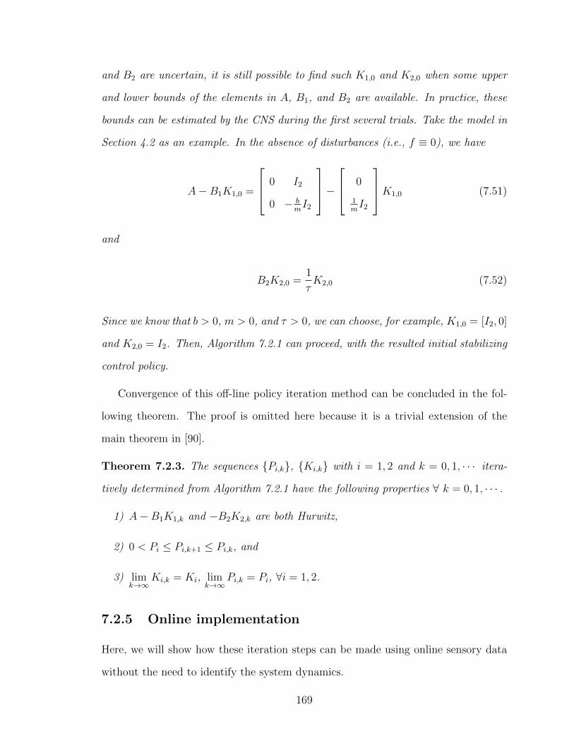
and B2 are uncertain, it is still possible to find such K1,0 and K2,0 when some upper
and lower bounds of the elements in A, B1, and B2 are available. In practice, these
bounds can be estimated by the CNS during the first several trials. Take the model in
Section 4.2 as an example. In the absence of disturbances (i.e., f ≡ 0), we have
A−B1K1,0 =
0 I2
0 − bmI2
−
0
1mI2
K1,0 (7.51)
and
B2K2,0 =1
τK2,0 (7.52)
Since we know that b > 0, m > 0, and τ > 0, we can choose, for example, K1,0 = [I2, 0]
and K2,0 = I2. Then, Algorithm 7.2.1 can proceed, with the resulted initial stabilizing
control policy.
Convergence of this off-line policy iteration method can be concluded in the fol-
lowing theorem. The proof is omitted here because it is a trivial extension of the
main theorem in [90].
Theorem 7.2.3. The sequences Pi,k, Ki,k with i = 1, 2 and k = 0, 1, · · · itera-
tively determined from Algorithm 7.2.1 have the following properties ∀ k = 0, 1, · · · .
1) A−B1K1,k and −B2K2,k are both Hurwitz,
2) 0 < Pi ≤ Pi,k+1 ≤ Pi,k, and
3) limk→∞
Ki,k = Ki, limk→∞
Pi,k = Pi, ∀i = 1, 2.
7.2.5 Online implementation
Here, we will show how these iteration steps can be made using online sensory data
without the need to identify the system dynamics.
169
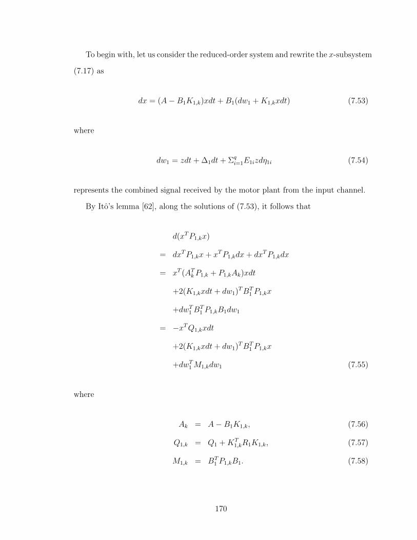
To begin with, let us consider the reduced-order system and rewrite the x-subsystem
(7.17) as
dx = (A−B1K1,k)xdt+B1(dw1 +K1,kxdt) (7.53)
where
dw1 = zdt+ ∆1dt+ Σqi=1E1izdη1i (7.54)
represents the combined signal received by the motor plant from the input channel.
By Ito’s lemma [62], along the solutions of (7.53), it follows that
d(xTP1,kx)
= dxTP1,kx+ xTP1,kdx+ dxTP1,kdx
= xT (ATkP1,k + P1,kAk)xdt
+2(K1,kxdt+ dw1)TBT1 P1,kx
+dwT1 BT1 P1,kB1dw1
= −xTQ1,kxdt
+2(K1,kxdt+ dw1)TBT1 P1,kx
+dwT1 M1,kdw1 (7.55)
where
Ak = A−B1K1,k, (7.56)
Q1,k = Q1 +KT1,kR1K1,k, (7.57)
M1,k = BT1 P1,kB1. (7.58)
170

Next, integrating both sides of (7.55) from t to t+ δt, we obtain
x(t+ δt)TP1,kx(t+ δt)− x(t)TP1,kx(t)
= −∫ t+δt
t
xTQ1,kxdt+
∫ t+δt
t
dwT1 M1,kdw1
+2
∫ t+δt
t
(K1,kxdt+ dw1)TR1K1,k+1x (7.59)
We now show that given a matrix K1,k such that A − B1K1,k is Hurwitz, a pair
of matrices (P1,k, K1,k+1), with P1,k = P T1,k > 0, satisfying (7.47) and (7.50) can be
uniquely determined without knowing A or B1 . To this end, we define the following
two operators:
P ∈ Rn×n → ν (P ) ∈ R12n(n+1)
x ∈ Rn → µ (x) ∈ R12n(n+1)
where
ν (P ) = [p11, 2p12, · · · , 2p1n, p22, 2p23, · · · , 2pn−1,n, pnn]T ,
µ (x) = [x21, x1x2, · · · , x1xn, x
22, x2x3, · · · , xn−1xn, x
2n]T .
In addition, by Kronecker product representation [56], we have
(K1,kxdt+ dw1)TR1K1,k+1x
= [x⊗R1(K1,kxdt+ dw1)]T vec(K1,k+1).
Further, for a sufficiently large positive integer lk > 0, we define the following two
171
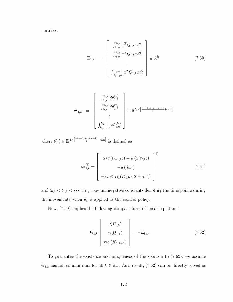
matrices.
Ξ1,k =
∫ t1,kt0,k
xTQ1,kxdt∫ t2,kt1,k
xTQ1,kxdt
...∫ tlk,ktlk−1,k
xTQ1,kxdt
∈ Rlk (7.60)
Θ1,k =
∫ t1,kt0,k
dθ(1)1,k
∫ t2,kt1,k
dθ(2)1,k
...∫ tlk,ktlk−1,k
dθ(lk)1,k
∈ Rlk×[n(n+1)+m(m+1)
2+mn]
where θ(i)1,k ∈ R1×[n(n+1)+m(m+1)
2+mn] is defined as
dθ(i)1,k =
µ (x(ti+1,k))− µ (x(ti,k))
−µ (dw1)
−2x⊗R1(K1,kxdt+ dw1)
T
(7.61)
and t0,k < t1,k < · · · < tlk,k are nonnegative constants denoting the time points during
the movements when uk is applied as the control policy.
Now, (7.59) implies the following compact form of linear equations
Θ1,k
ν(P1,k)
ν(M1,k)
vec (K1,k+1)
= −Ξ1,k. (7.62)
To guarantee the existence and uniqueness of the solution to (7.62), we assume
Θ1,k has full column rank for all k ∈ Z+. As a result, (7.62) can be directly solved as
172
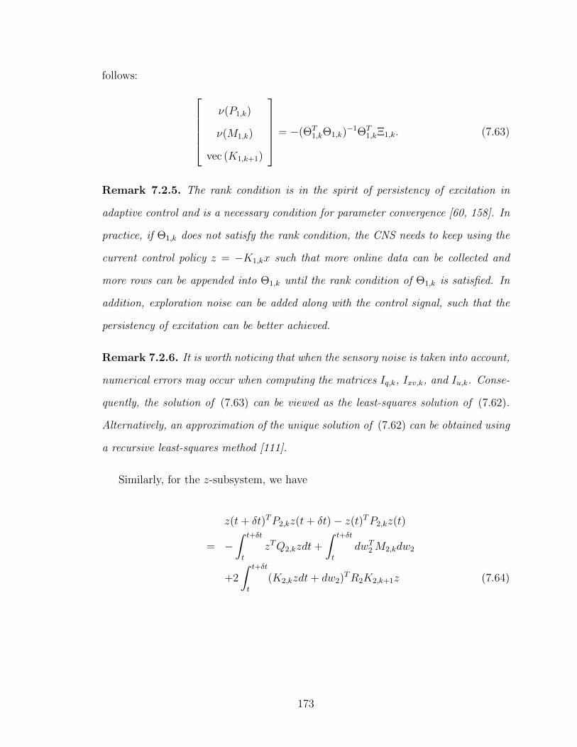
follows:
ν(P1,k)
ν(M1,k)
vec (K1,k+1)
= −(ΘT1,kΘ1,k)
−1ΘT1,kΞ1,k. (7.63)
Remark 7.2.5. The rank condition is in the spirit of persistency of excitation in
adaptive control and is a necessary condition for parameter convergence [60, 158]. In
practice, if Θ1,k does not satisfy the rank condition, the CNS needs to keep using the
current control policy z = −K1,kx such that more online data can be collected and
more rows can be appended into Θ1,k until the rank condition of Θ1,k is satisfied. In
addition, exploration noise can be added along with the control signal, such that the
persistency of excitation can be better achieved.
Remark 7.2.6. It is worth noticing that when the sensory noise is taken into account,
numerical errors may occur when computing the matrices Iq,k, Ixv,k, and Iu,k. Conse-
quently, the solution of (7.63) can be viewed as the least-squares solution of (7.62).
Alternatively, an approximation of the unique solution of (7.62) can be obtained using
a recursive least-squares method [111].
Similarly, for the z-subsystem, we have
z(t+ δt)TP2,kz(t+ δt)− z(t)TP2,kz(t)
= −∫ t+δt
t
zTQ2,kzdt+
∫ t+δt
t
dwT2 M2,kdw2
+2
∫ t+δt
t
(K2,kzdt+ dw2)TR2K2,k+1z (7.64)
173
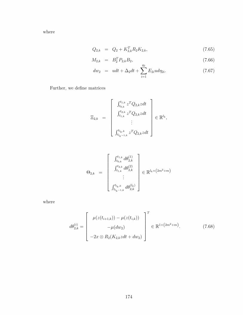
where
Q2,k = Q2 +KT2,kR2K2,k, (7.65)
M2,k = BT2 P2,kB2, (7.66)
dw2 = udt+ ∆2dt+
q2∑
i=1
E2iudη2i. (7.67)
Further, we define matrices
Ξ2,k =
∫ t1,kt0,k
zTQ2,kzdt∫ t2,kt1,k
zTQ2,kzdt
...∫ tlk,ktlk−1,k
zTQ2,kzdt
∈ Rlk ,
Θ2,k =
∫ t1,kt0,k
dθ(1)2,k
∫ t2,kt1,k
dθ(2)2,k
...∫ tlk,ktlk−1,k
dθ(lk)2,k
∈ Rlk×(2m2+m)
where
dθ(i)2,k =
µ(z(ti+1,k))− µ(z(ti,k))
−µ(dw2)
−2x⊗R2(K2,kzdt+ dw2)
T
∈ R1×(2m2+m). (7.68)
174
Then, the unknown matrices in each iteration step can be directly solved, that is,
ν(P2,k)
ν(M2,k)
vec (K2,k+1)
= −(ΘT2,kΘ2,k)
−1ΘT2,kΞ2,k. (7.69)
The motor learning algorithm based on the proposed RADP theory can thus be
summarized as follows:
Algorithm 7.2.2 RADP-based motor learning algorithm
1: Apply an initial control policy in the form of (7.46), and let k = 0.2: Collect online sensory data to compute the matrices Θi,k and Ξi,k with i = 1, 2.3: Let k ← k + 1, and update the control policy using (7.63) and (7.69). Then,
apply the new control policy (7.49) to the motor system.4: Go to Step 2.
Corollary 7.2.1. Suppose Θi,k is of full-column rank for all i = 1, 2 and k = 0, 1, · · · .
Then, the control policies obtained from Algorithm 7.2.2 converge to the robust optimal
control policy (7.38).
Proof. This corollary is a direct result from Theorem 7.2.3 by noticing that the ma-
trices Pi,k , Mi,k and Ki,k+1 obtained from Algorithm 7.2.1 and Algorithm 7.2.2 are
equivalent for i = 1, 2, and k = 0, 1, · · · .
Remark 7.2.7. It is worth noticing that the past measurements on dw1 and dw2 are
assumed available for online learning purpose. In the following sections, we will see
that they correspond to the combined control signals received by the muscles. These
signals can be measured by the muscle spindle and the Golgi tendon organs, and can
be transmitted to the brain via the peripheral nervous systems (PNS).
175
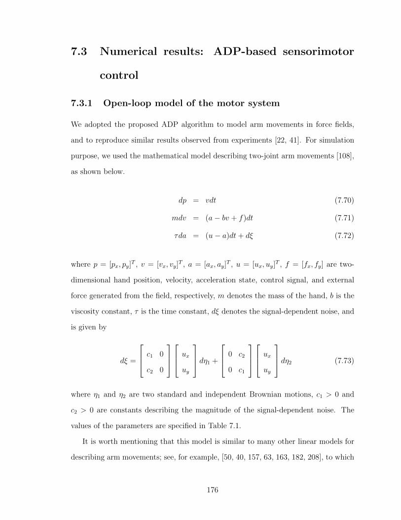
7.3 Numerical results: ADP-based sensorimotor
control
7.3.1 Open-loop model of the motor system
We adopted the proposed ADP algorithm to model arm movements in force fields,
and to reproduce similar results observed from experiments [22, 41]. For simulation
purpose, we used the mathematical model describing two-joint arm movements [108],
as shown below.
dp = vdt (7.70)
mdv = (a− bv + f)dt (7.71)
τda = (u− a)dt+ dξ (7.72)
where p = [px, py]T , v = [vx, vy]
T , a = [ax, ay]T , u = [ux, uy]
T , f = [fx, fy] are two-
dimensional hand position, velocity, acceleration state, control signal, and external
force generated from the field, respectively, m denotes the mass of the hand, b is the
viscosity constant, τ is the time constant, dξ denotes the signal-dependent noise, and
is given by
dξ =
c1 0
c2 0
ux
uy
dη1 +
0 c2
0 c1
ux
uy
dη2 (7.73)
where η1 and η2 are two standard and independent Brownian motions, c1 > 0 and
c2 > 0 are constants describing the magnitude of the signal-dependent noise. The
values of the parameters are specified in Table 7.1.
It is worth mentioning that this model is similar to many other linear models for
describing arm movements; see, for example, [50, 40, 157, 63, 163, 182, 208], to which
176

Table 7.1: Parameters of the linear modelParameters Description Value Dimension
m Hand mass 1.3 kgb Viscosity constant 10 N· s/mτ Time constant 0.05 sc1 Noise magnitude 0.075c2 Noise magnitude 0.025
our ADP theory is also applicable.
7.3.2 Determining the initial stabilizing control policy
The proposed ADP-based online learning methodology requires an initial stabilizing
control policy. To be more specific, we need to find an initial stabilizing feedback gain
matrix K0 ∈ R2×6, such that the closed-loop matrix A−BK0 is Hurwitz. By robust
control theory [207], it is possible to find such a matrix K0 if upper and lower bounds
of the elements in both A and B are available and the pair (A,B) is stabilizable.
Indeed, these bounds can be estimated by the CNS during the first several trials.
For example, in the absence of disturbances (i.e., f ≡ 0), we have
A−BK0 =
0 I2 0
0 − bmI2
1mI2
0 0 1τI2
−
0
0
1τI2
K0 (7.74)
Then, the first several trials in the NF can be interpreted as the exploration
of an initial stabilizing feedback gain matrix K0, by estimating the bounds on the
parameters b, m, and τ , and solving a robust control problem. Indeed, if the CNS
finds out that b ∈ [−8, 12], m ∈ [1, 1.5], and τ ∈ [0.03, 0.07] through the first several
177
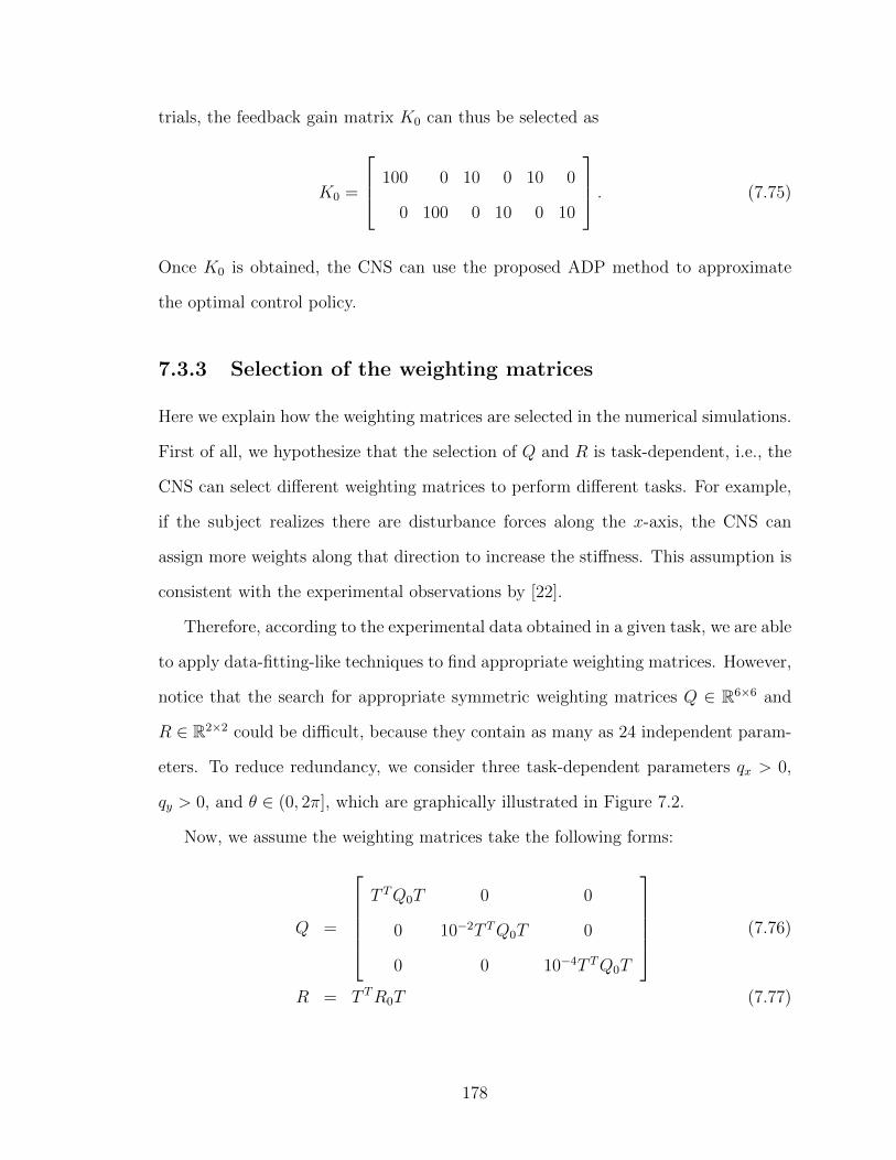
trials, the feedback gain matrix K0 can thus be selected as
K0 =
100 0 10 0 10 0
0 100 0 10 0 10
. (7.75)
Once K0 is obtained, the CNS can use the proposed ADP method to approximate
the optimal control policy.
7.3.3 Selection of the weighting matrices
Here we explain how the weighting matrices are selected in the numerical simulations.
First of all, we hypothesize that the selection of Q and R is task-dependent, i.e., the
CNS can select different weighting matrices to perform different tasks. For example,
if the subject realizes there are disturbance forces along the x-axis, the CNS can
assign more weights along that direction to increase the stiffness. This assumption is
consistent with the experimental observations by [22].
Therefore, according to the experimental data obtained in a given task, we are able
to apply data-fitting-like techniques to find appropriate weighting matrices. However,
notice that the search for appropriate symmetric weighting matrices Q ∈ R6×6 and
R ∈ R2×2 could be difficult, because they contain as many as 24 independent param-
eters. To reduce redundancy, we consider three task-dependent parameters qx > 0,
qy > 0, and θ ∈ (0, 2π], which are graphically illustrated in Figure 7.2.
Now, we assume the weighting matrices take the following forms:
Q =
T TQ0T 0 0
0 10−2T TQ0T 0
0 0 10−4T TQ0T
(7.76)
R = T TR0T (7.77)
178
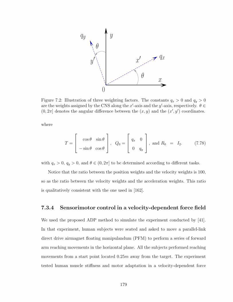
x
y
x′y′
0
θ
qx
qy
θ
Figure 7.2: Illustration of three weighting factors. The constants qx > 0 and qy > 0are the weights assigned by the CNS along the x′-axis and the y′-axis, respectively. θ ∈(0, 2π] denotes the angular difference between the (x, y) and the (x′, y′) coordinates.
where
T =
cos θ sin θ
− sin θ cos θ
, Q0 =
qx 0
0 qy
, and R0 = I2. (7.78)
with qx > 0, qy > 0, and θ ∈ (0, 2π] to be determined according to different tasks.
Notice that the ratio between the position weights and the velocity weights is 100,
so as the ratio between the velocity weights and the acceleration weights. This ratio
is qualitatively consistent with the one used in [162].
7.3.4 Sensorimotor control in a velocity-dependent force field
We used the proposed ADP method to simulate the experiment conducted by [41].
In that experiment, human subjects were seated and asked to move a parallel-link
direct drive airmagnet floating manipulandum (PFM) to perform a series of forward
arm reaching movements in the horizontal plane. All the subjects performed reaching
movements from a start point located 0.25m away from the target. The experiment
tested human muscle stiffness and motor adaptation in a velocity-dependent force
179
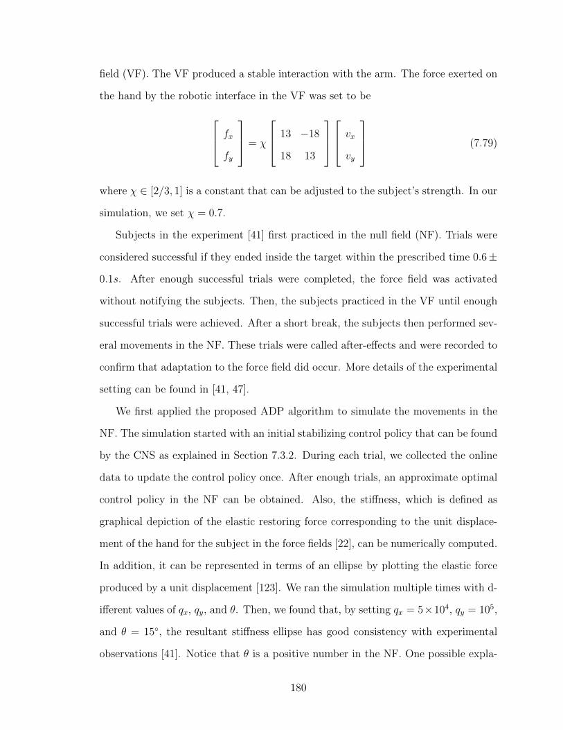
field (VF). The VF produced a stable interaction with the arm. The force exerted on
the hand by the robotic interface in the VF was set to be
fx
fy
= χ
13 −18
18 13
vx
vy
(7.79)
where χ ∈ [2/3, 1] is a constant that can be adjusted to the subject’s strength. In our
simulation, we set χ = 0.7.
Subjects in the experiment [41] first practiced in the null field (NF). Trials were
considered successful if they ended inside the target within the prescribed time 0.6±
0.1s. After enough successful trials were completed, the force field was activated
without notifying the subjects. Then, the subjects practiced in the VF until enough
successful trials were achieved. After a short break, the subjects then performed sev-
eral movements in the NF. These trials were called after-effects and were recorded to
confirm that adaptation to the force field did occur. More details of the experimental
setting can be found in [41, 47].
We first applied the proposed ADP algorithm to simulate the movements in the
NF. The simulation started with an initial stabilizing control policy that can be found
by the CNS as explained in Section 7.3.2. During each trial, we collected the online
data to update the control policy once. After enough trials, an approximate optimal
control policy in the NF can be obtained. Also, the stiffness, which is defined as
graphical depiction of the elastic restoring force corresponding to the unit displace-
ment of the hand for the subject in the force fields [22], can be numerically computed.
In addition, it can be represented in terms of an ellipse by plotting the elastic force
produced by a unit displacement [123]. We ran the simulation multiple times with d-
ifferent values of qx, qy, and θ. Then, we found that, by setting qx = 5×10⁴, qy = 105,
and θ = 15, the resultant stiffness ellipse has good consistency with experimental
observations [41]. Notice that θ is a positive number in the NF. One possible expla-
180
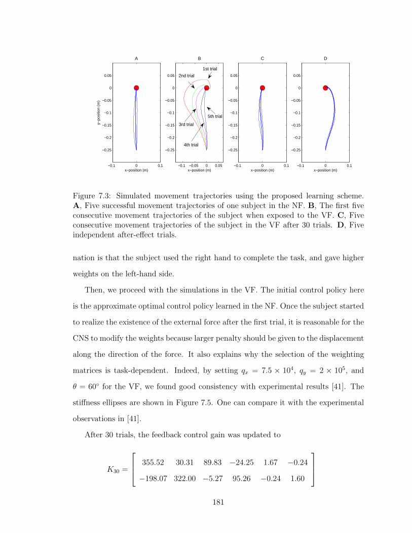
−0.1 −0.05 0 0.05
−0.25
−0.2
−0.15
−0.1
−0.05
0
0.05
B
x−position (m)−0.1 0 0.1
−0.25
−0.2
−0.15
−0.1
−0.05
0
0.05
x−position (m)
y−po
sitio
n (m
)
A
−0.1 0 0.1
−0.25
−0.2
−0.15
−0.1
−0.05
0
0.05
C
x−position (m)−0.1 0 0.1
−0.25
−0.2
−0.15
−0.1
−0.05
0
0.05
D
x−position (m)
4th trial
3rd trial
2nd trial
5th trial
1st trial
Figure 7.3: Simulated movement trajectories using the proposed learning scheme.A, Five successful movement trajectories of one subject in the NF. B, The first fiveconsecutive movement trajectories of the subject when exposed to the VF. C, Fiveconsecutive movement trajectories of the subject in the VF after 30 trials. D, Fiveindependent after-effect trials.
nation is that the subject used the right hand to complete the task, and gave higher
weights on the left-hand side.
Then, we proceed with the simulations in the VF. The initial control policy here
is the approximate optimal control policy learned in the NF. Once the subject started
to realize the existence of the external force after the first trial, it is reasonable for the
CNS to modify the weights because larger penalty should be given to the displacement
along the direction of the force. It also explains why the selection of the weighting
matrices is task-dependent. Indeed, by setting qx = 7.5 × 10⁴, qy = 2 × 10⁵, and
θ = 60 for the VF, we found good consistency with experimental results [41]. The
stiffness ellipses are shown in Figure 7.5. One can compare it with the experimental
observations in [41].
After 30 trials, the feedback control gain was updated to
K30 =
355.52 30.31 89.83 −24.25 1.67 −0.24
−198.07 322.00 −5.27 95.26 −0.24 1.60
181
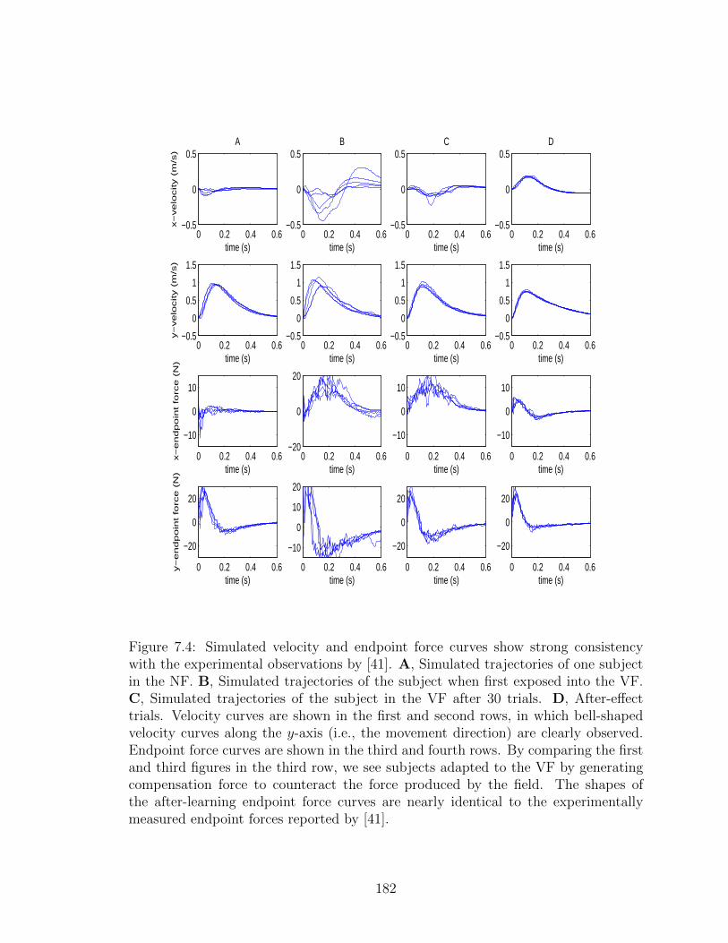
0 0.2 0.4 0.6−0.5
0
0.5
time (s)
B
0 0.2 0.4 0.6−0.5
0
0.5
1
1.5
time (s)
0 0.2 0.4 0.6−20
0
20
time (s)
0 0.2 0.4 0.6
−10
0
10
20
time (s)
0 0.2 0.4 0.6−0.5
0
0.5
time (s)
x−
ve
locity (
m/s
)
A
0 0.2 0.4 0.6−0.5
0
0.5
1
1.5
time (s)
y−
ve
locity (
m/s
)
0 0.2 0.4 0.6
−10
0
10
time (s)
x−
en
dp
oin
t fo
rce
(N
)
0 0.2 0.4 0.6
−20
0
20
time (s)
y−
en
dp
oin
t fo
rce
(N
)
0 0.2 0.4 0.6−0.5
0
0.5
time (s)
C
0 0.2 0.4 0.6−0.5
0
0.5
1
1.5
time (s)
0 0.2 0.4 0.6
−10
0
10
time (s)
0 0.2 0.4 0.6
−20
0
20
time (s)
0 0.2 0.4 0.6−0.5
0
0.5
time (s)
D
0 0.2 0.4 0.6−0.5
0
0.5
1
1.5
time (s)
0 0.2 0.4 0.6
−10
0
10
time (s)
0 0.2 0.4 0.6
−20
0
20
time (s)
Figure 7.4: Simulated velocity and endpoint force curves show strong consistencywith the experimental observations by [41]. A, Simulated trajectories of one subjectin the NF. B, Simulated trajectories of the subject when first exposed into the VF.C, Simulated trajectories of the subject in the VF after 30 trials. D, After-effecttrials. Velocity curves are shown in the first and second rows, in which bell-shapedvelocity curves along the y-axis (i.e., the movement direction) are clearly observed.Endpoint force curves are shown in the third and fourth rows. By comparing the firstand third figures in the third row, we see subjects adapted to the VF by generatingcompensation force to counteract the force produced by the field. The shapes ofthe after-learning endpoint force curves are nearly identical to the experimentallymeasured endpoint forces reported by [41].
182
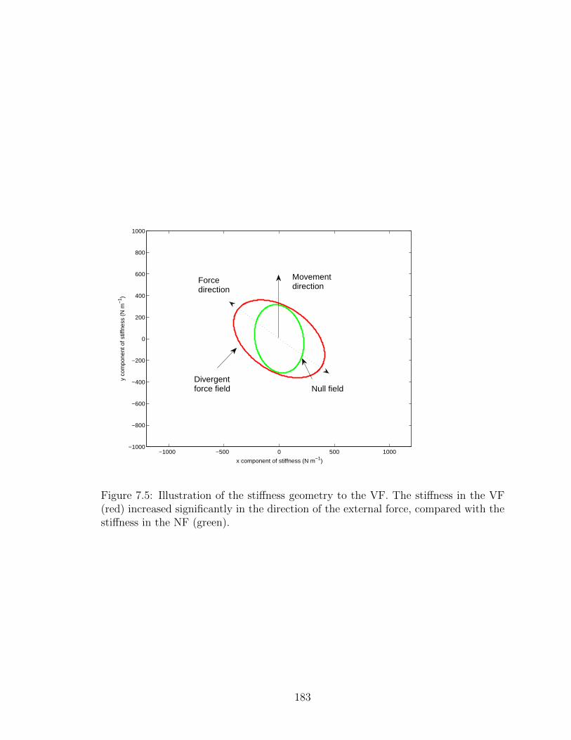
−1000 −500 0 500 1000−1000
−800
−600
−400
−200
0
200
400
600
800
1000
x component of stiffness (N m−1)
y co
mpo
nent
of s
tiffn
ess
(N m
−1)
Null field
Movementdirection
Forcedirection
Divergentforce field
Figure 7.5: Illustration of the stiffness geometry to the VF. The stiffness in the VF(red) increased significantly in the direction of the external force, compared with thestiffness in the NF (green).
183

For comparison, the optimal feedback gain matrix is provided as follows:
K∗ =
358.32 30.89 90.17 −24.15 1.67 −0.24
−200.92 324.49 −5.65 95.63 −0.24 1.60
.
The simulated movement trajectories, the velocity curves, and the endpoint force
curves are shown in Figures 7.3 and 7.4. It can be seen that the simulated move-
ment trajectories in the NF are approximately straight lines, and the velocity curves
along the y-axis are bell-shaped curves. These simulation results are consistent with
experimental observations as well as the curves produced by the previous models
[120, 40, 162]. After the subject was exposed to the VF, the first trial was simulated
with the same feedback control policy as in the NF. This is because subjects in the
experiment were not notified when the external force was activated. Apparently, this
control policy was not optimal because the system dynamics was changed and the
cost function was also different. Then, the ADP algorithm proceeded. In Figure 7.3,
we see the first trial gives a movement trajectory which deviated far away from the
straight path but eventually reached the target. Motor adaptation can be observed
by comparing the first five consecutive trials. After 30 trials, the movement trajec-
tories return to be straight lines, and the velocity curves become bell-shaped again.
It implies that after 30 trials in the VF, the CNS can learn well the optimal control
policy using real-time data, without knowing or using the precise system parameters.
Finally, our numerical study shows clearly the after-effects of the subject behavior
when the VF was suddenly de-activated.
To better illustrate the learning behavior in the VF, we define the movement time
tf of each trial as the time duration from the beginning of the trial until the hand-
path enters and remains in the target area. Then, the movement times and distance
were calculated and are shown in Figure 7.6.
184
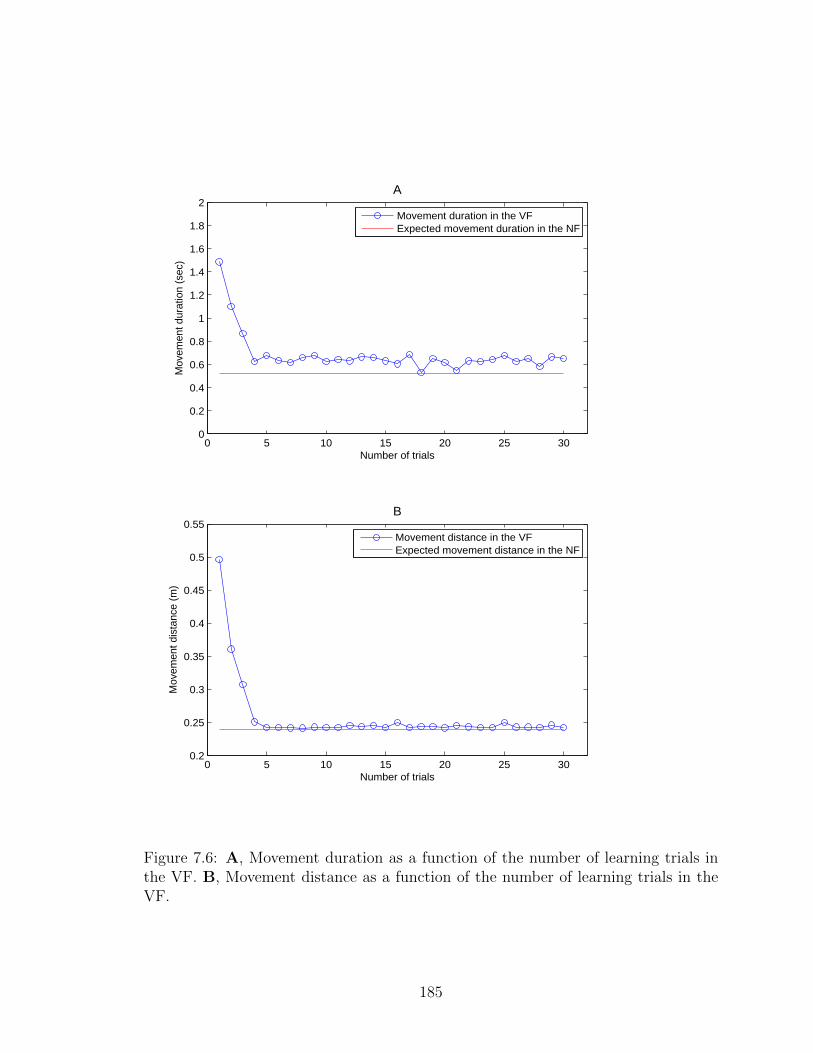
0 5 10 15 20 25 300
0.2
0.4
0.6
0.8
1
1.2
1.4
1.6
1.8
2
Number of trials
Mov
emen
t dur
atio
n (s
ec)
A
0 5 10 15 20 25 300.2
0.25
0.3
0.35
0.4
0.45
0.5
0.55
Number of trials
Mov
emen
t dis
tanc
e (m
)
B
Movement duration in the VFExpected movement duration in the NF
Movement distance in the VFExpected movement distance in the NF
Figure 7.6: A, Movement duration as a function of the number of learning trials inthe VF. B, Movement distance as a function of the number of learning trials in theVF.
185
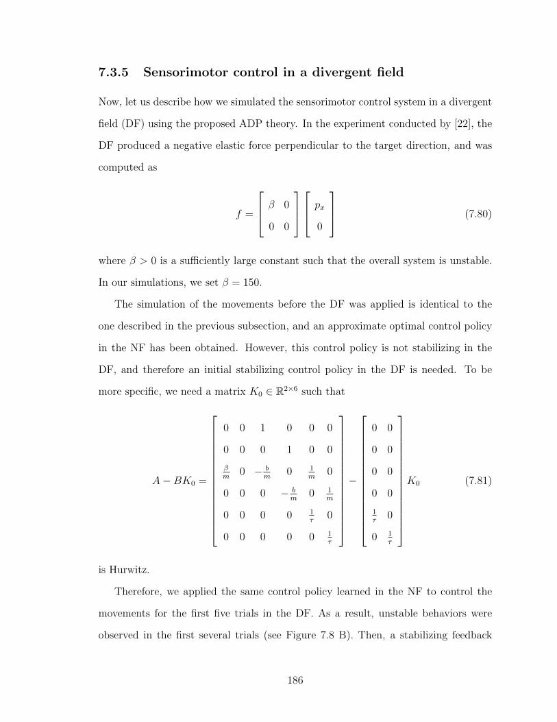
7.3.5 Sensorimotor control in a divergent field
Now, let us describe how we simulated the sensorimotor control system in a divergent
field (DF) using the proposed ADP theory. In the experiment conducted by [22], the
DF produced a negative elastic force perpendicular to the target direction, and was
computed as
f =
β 0
0 0
px
0
(7.80)
where β > 0 is a sufficiently large constant such that the overall system is unstable.
In our simulations, we set β = 150.
The simulation of the movements before the DF was applied is identical to the
one described in the previous subsection, and an approximate optimal control policy
in the NF has been obtained. However, this control policy is not stabilizing in the
DF, and therefore an initial stabilizing control policy in the DF is needed. To be
more specific, we need a matrix K0 ∈ R2×6 such that
A−BK0 =
0 0 1 0 0 0
0 0 0 1 0 0
βm
0 − bm
0 1m
0
0 0 0 − bm
0 1m
0 0 0 0 1τ
0
0 0 0 0 0 1τ
−
0 0
0 0
0 0
0 0
1τ
0
0 1τ
K0 (7.81)
is Hurwitz.
Therefore, we applied the same control policy learned in the NF to control the
movements for the first five trials in the DF. As a result, unstable behaviors were
observed in the first several trials (see Figure 7.8 B). Then, a stabilizing feedback
186
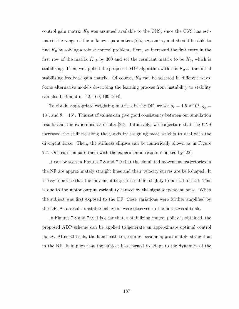
control gain matrix K0 was assumed available to the CNS, since the CNS has esti-
mated the range of the unknown parameters β, b, m, and τ , and should be able to
find K0 by solving a robust control problem. Here, we increased the first entry in the
first row of the matrix Knf by 300 and set the resultant matrix to be K0, which is
stabilizing. Then, we applied the proposed ADP algorithm with this K0 as the initial
stabilizing feedback gain matrix. Of course, K0 can be selected in different ways.
Some alternative models describing the learning process from instability to stability
can also be found in [42, 160, 199, 208].
To obtain appropriate weighting matrices in the DF, we set qx = 1.5× 10⁵, qy =
105, and θ = 15. This set of values can give good consistency between our simulation
results and the experimental results [22]. Intuitively, we conjecture that the CNS
increased the stiffness along the y-axis by assigning more weights to deal with the
divergent force. Then, the stiffness ellipses can be numerically shown as in Figure
7.7. One can compare them with the experimental results reported by [22].
It can be seen in Figures 7.8 and 7.9 that the simulated movement trajectories in
the NF are approximately straight lines and their velocity curves are bell-shaped. It
is easy to notice that the movement trajectories differ slightly from trial to trial. This
is due to the motor output variability caused by the signal-dependent noise. When
the subject was first exposed to the DF, these variations were further amplified by
the DF. As a result, unstable behaviors were observed in the first several trials.
In Figures 7.8 and 7.9, it is clear that, a stabilizing control policy is obtained, the
proposed ADP scheme can be applied to generate an approximate optimal control
policy. After 30 trials, the hand-path trajectories became approximately straight as
in the NF. It implies that the subject has learned to adapt to the dynamics of the
187
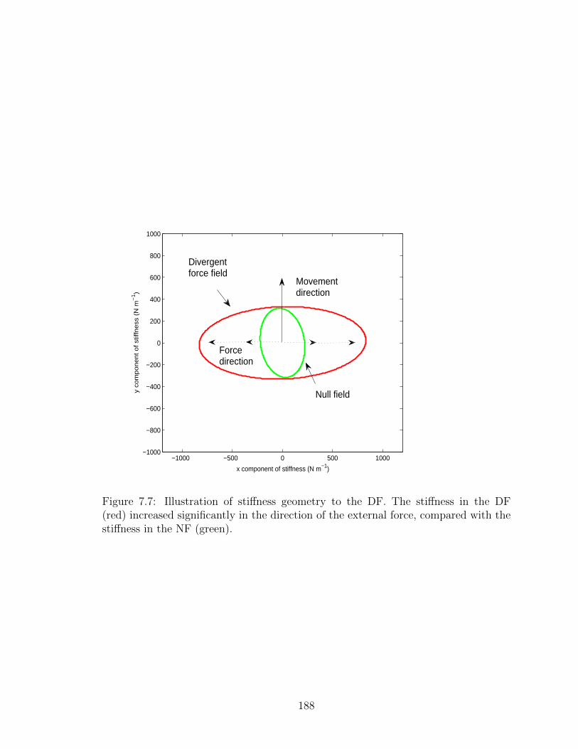
−1000 −500 0 500 1000−1000
−800
−600
−400
−200
0
200
400
600
800
1000
x component of stiffness (N m−1)
y co
mp
on
en
t o
f st
iffn
ess
(N
m−
1)
Divergentforce field
Null field
Movementdirection
Forcedirection
Figure 7.7: Illustration of stiffness geometry to the DF. The stiffness in the DF(red) increased significantly in the direction of the external force, compared with thestiffness in the NF (green).
188
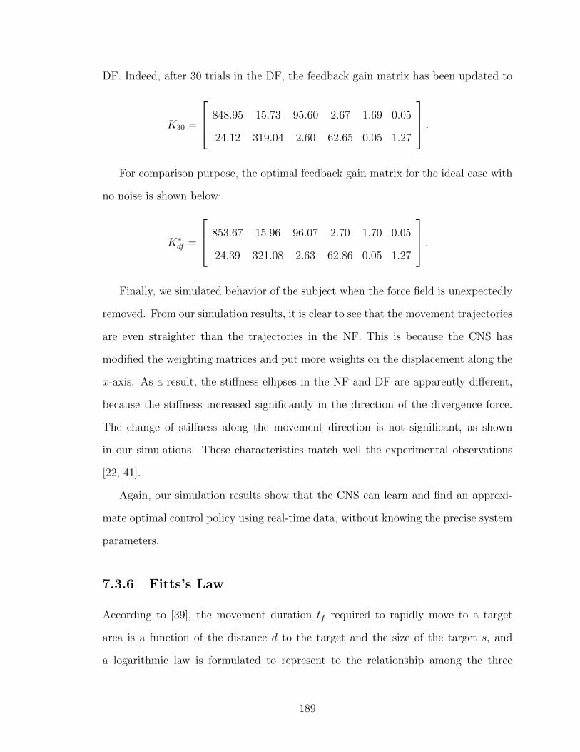
DF. Indeed, after 30 trials in the DF, the feedback gain matrix has been updated to
K30 =
848.95 15.73 95.60 2.67 1.69 0.05
24.12 319.04 2.60 62.65 0.05 1.27
.
For comparison purpose, the optimal feedback gain matrix for the ideal case with
no noise is shown below:
K∗df =
853.67 15.96 96.07 2.70 1.70 0.05
24.39 321.08 2.63 62.86 0.05 1.27
.
Finally, we simulated behavior of the subject when the force field is unexpectedly
removed. From our simulation results, it is clear to see that the movement trajectories
are even straighter than the trajectories in the NF. This is because the CNS has
modified the weighting matrices and put more weights on the displacement along the
x-axis. As a result, the stiffness ellipses in the NF and DF are apparently different,
because the stiffness increased significantly in the direction of the divergence force.
The change of stiffness along the movement direction is not significant, as shown
in our simulations. These characteristics match well the experimental observations
[22, 41].
Again, our simulation results show that the CNS can learn and find an approxi-
mate optimal control policy using real-time data, without knowing the precise system
parameters.
7.3.6 Fitts’s Law
According to [39], the movement duration tf required to rapidly move to a target
area is a function of the distance d to the target and the size of the target s, and
a logarithmic law is formulated to represent to the relationship among the three
189
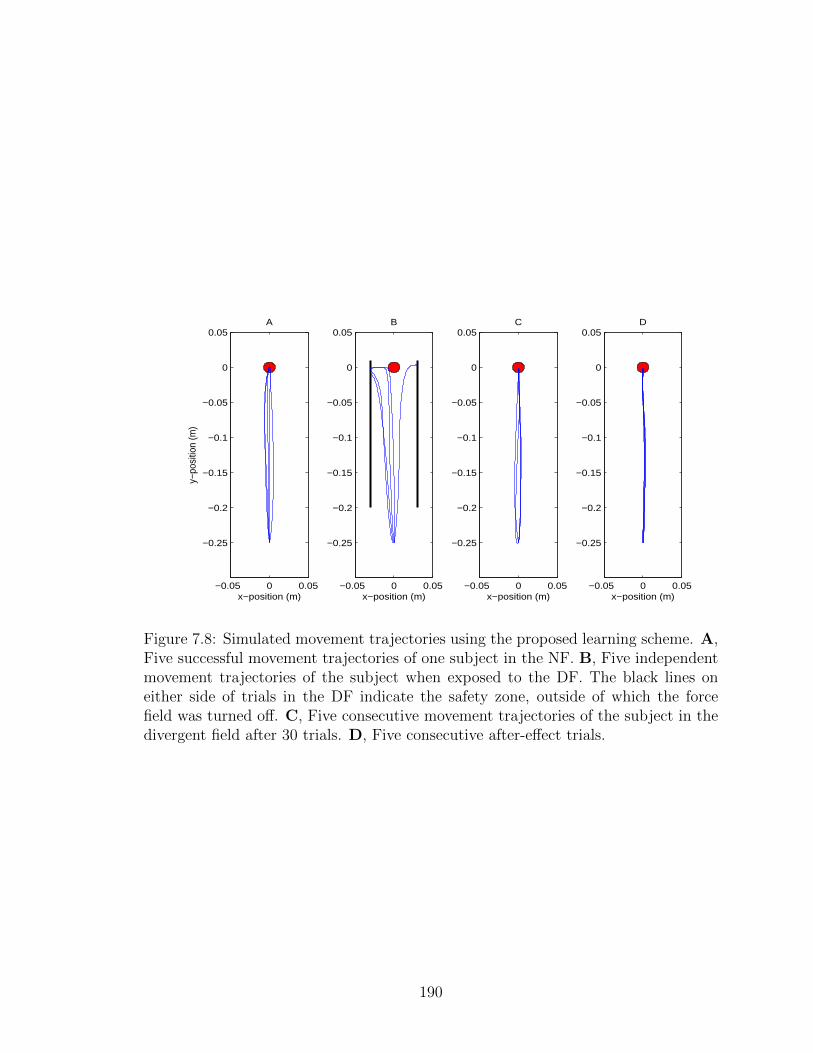
−0.05 0 0.05
−0.25
−0.2
−0.15
−0.1
−0.05
0
0.05
x−position (m)
y−po
sitio
n (m
)
A
−0.05 0 0.05
−0.25
−0.2
−0.15
−0.1
−0.05
0
0.05B
x−position (m)−0.05 0 0.05
−0.25
−0.2
−0.15
−0.1
−0.05
0
0.05C
x−position (m)−0.05 0 0.05
−0.25
−0.2
−0.15
−0.1
−0.05
0
0.05D
x−position (m)
Figure 7.8: Simulated movement trajectories using the proposed learning scheme. A,Five successful movement trajectories of one subject in the NF. B, Five independentmovement trajectories of the subject when exposed to the DF. The black lines oneither side of trials in the DF indicate the safety zone, outside of which the forcefield was turned off. C, Five consecutive movement trajectories of the subject in thedivergent field after 30 trials. D, Five consecutive after-effect trials.
190

0 0.2 0.4 0.6−0.5
0
0.5
time (s)
x−
ve
locity (
m/s
)
A
0 0.2 0.4 0.6−0.5
0
0.5
1
1.5
time (s)
y−
ve
locity (
m/s
)
0 0.2 0.4 0.6
−10
0
10
time (s)
x−
en
dp
oin
t fo
rce
(N
)
0 0.2 0.4 0.6
−20
0
20
time (s)
y−
en
dp
oin
t fo
rce
(N
)
0 0.2 0.4 0.6−0.5
0
0.5
time (s)
B
0 0.2 0.4 0.6−0.5
0
0.5
1
1.5
time (s)
0 0.2 0.4 0.6
−20
0
20
time (s)
0 0.2 0.4 0.6−50
0
50
time (s)
0 0.2 0.4 0.6−0.5
0
0.5
time (s)
C
0 0.2 0.4 0.6−0.5
0
0.5
1
1.5
time (s)
0 0.2 0.4 0.6
−10
0
10
time (s)
0 0.2 0.4 0.6
−20
0
20
time (s)
0 0.2 0.4 0.6−0.5
0
0.5
time (s)
D
0 0.2 0.4 0.6−0.5
0
0.5
1
1.5
time (s)
0 0.2 0.4 0.6
−10
0
10
time (s)
0 0.2 0.4 0.6
−20
0
20
time (s)
Figure 7.9: Simulated velocity and endpoint force curves using the proposed learningscheme. A, Simulated trajectories of one subject in the NF. B, Simulated trajectoriesof the subject when first exposed into the DF. Some trials were terminated earlierthan 0.6s because they went out of the save zone. C, Simulated trajectories of thesubject in the divergent force field after 30 trials. D, After-effect trials. Velocitycurves are shown in the first and second rows, in which bell-shaped velocity curvesalong the y-axis (i.e., the movement direction) are clearly observed. Endpoint forcecurves are shown in the third and fourth rows, in which we see subjects adapted tothe DF by generating compensation force in the x-direction to counteract the forceproduced by the DF. In addition, the endpoint force curves are nearly identical tothe experimentally measured data [22].
191
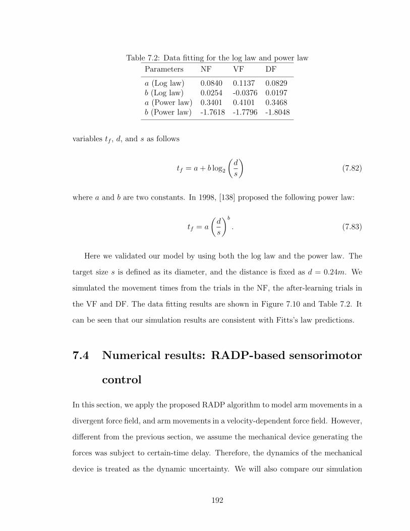
Table 7.2: Data fitting for the log law and power law
Parameters NF VF DF
a (Log law) 0.0840 0.1137 0.0829b (Log law) 0.0254 -0.0376 0.0197a (Power law) 0.3401 0.4101 0.3468b (Power law) -1.7618 -1.7796 -1.8048
variables tf , d, and s as follows
tf = a+ b log2
(d
s
)(7.82)
where a and b are two constants. In 1998, [138] proposed the following power law:
tf = a
(d
s
)b. (7.83)
Here we validated our model by using both the log law and the power law. The
target size s is defined as its diameter, and the distance is fixed as d = 0.24m. We
simulated the movement times from the trials in the NF, the after-learning trials in
the VF and DF. The data fitting results are shown in Figure 7.10 and Table 7.2. It
can be seen that our simulation results are consistent with Fitts’s law predictions.
7.4 Numerical results: RADP-based sensorimotor
control
In this section, we apply the proposed RADP algorithm to model arm movements in a
divergent force field, and arm movements in a velocity-dependent force field. However,
different from the previous section, we assume the mechanical device generating the
forces was subject to certain-time delay. Therefore, the dynamics of the mechanical
device is treated as the dynamic uncertainty. We will also compare our simulation
192

1 2 3 4 5 6 70
0.1
0.2
0.3
0.4
0.5
0.6
0.7
0.8
log2(2d/s)
Mo
vem
en
t tim
e t
f (se
c)
A
Movement duration of each trialLeast−squares fit using the log law
0 1 2 3 4−2
−1.8
−1.6
−1.4
−1.2
−1
−0.8
−0.6
−0.4
−0.2
0
ln(d/s)
ln(t
f)
B
Movement duration of each trialLeast−squares fit using the power law
1 2 3 4 5 6 70
0.1
0.2
0.3
0.4
0.5
0.6
0.7
0.8
0.9
log2(2d/s)
Mo
ve
me
nt tim
e t
f (se
c)
C
0 1 2 3 4−2
−1.8
−1.6
−1.4
−1.2
−1
−0.8
−0.6
−0.4
−0.2
0
ln(d/s)
ln(t
f)
D
Movement duration of each trialLeast−squares fit using the log law
Movement duration of each trialLeast−squares fit using the power law
1 2 3 4 5 6 70
0.1
0.2
0.3
0.4
0.5
0.6
0.7
0.8
log2(2d/s)
Mo
ve
me
nt tim
e t
f (se
c)
E
0 1 2 3 4−2
−1.8
−1.6
−1.4
−1.2
−1
−0.8
−0.6
−0.4
−0.2
0
ln(d/s)
ln(t
f)
F
Movement duration of each trialLeast−squares fit using the log law
Movement duration of each trialLeast−squares fit using the power law
Figure 7.10: Log and power forms of Fitts’s law. Crosses in the first row, the secondrow, and the third row represent movement times simulated in the NF, the VF, andthe DF, respectively. Solid lines in A, C, E are least-squares fits using the log Fitts’slaw, and solid lines in B, D, F are the least-squares fits using the power Fitts’s law.
193
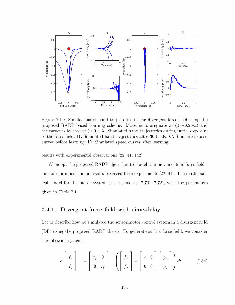
−0.05 0 0.05
−0.25
−0.2
−0.15
−0.1
−0.05
0
0.05
x−position (m)
y−po
sitio
n (m
)
A
−0.05 0 0.05
−0.25
−0.2
−0.15
−0.1
−0.05
0
0.05
x−position (m)
y−po
sitio
n (m
)
C
0 0.5 1 1.5−50
0
50
x−ve
loci
ty (
m/s
)
Time (sec)
B
0 0.5 1 1.5−50
0
50
y−ve
loci
ty (
m/s
)
Time (sec)
0 0.5 1−1
−0.5
0
0.5
1
x−ve
loci
ty (
m/s
)
Time (sec)
D
0 0.5 1−1
−0.5
0
0.5
1
y−ve
loci
ty (
m/s
)
Time (sec)
Figure 7.11: Simulations of hand trajectories in the divergent force field using theproposed RADP based learning scheme. Movements originate at (0,−0.25m) andthe target is located at (0, 0). A. Simulated hand trajectories during initial exposureto the force field. B. Simulated hand trajectories after 30 trials. C. Simulated speedcurves before learning. D. Simulated speed curves after learning.
results with experimental observations [22, 41, 142].
We adopt the proposed RADP algorithm to model arm movements in force fields,
and to reproduce similar results observed from experiments [22, 41]. The mathemat-
ical model for the motor system is the same as (7.70)-(7.72), with the parameters
given in Table 7.1.
7.4.1 Divergent force field with time-delay
Let us describe how we simulated the sensorimotor control system in a divergent field
(DF) using the proposed RADP theory. To generate such a force field, we consider
the following system.
d
fx
fy
= −
τf 0
0 τf
−1
fx
fy
−
β 0
0 0
px
py
dt (7.84)
194
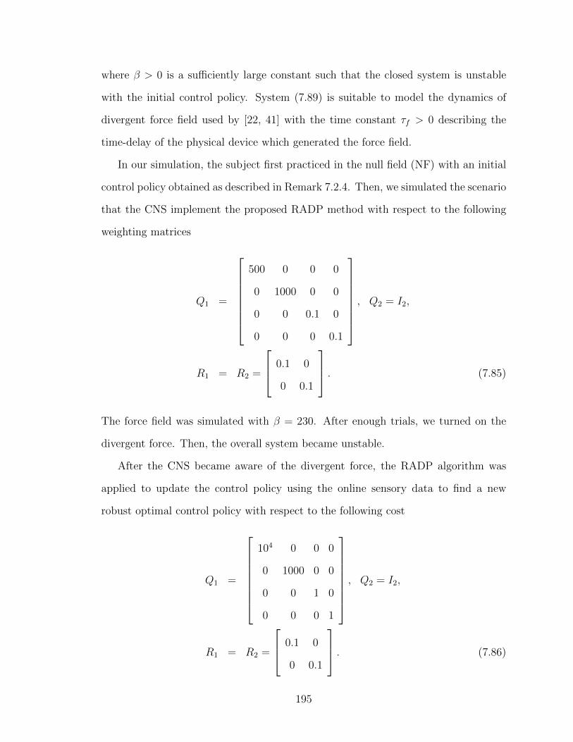
where β > 0 is a sufficiently large constant such that the closed system is unstable
with the initial control policy. System (7.89) is suitable to model the dynamics of
divergent force field used by [22, 41] with the time constant τf > 0 describing the
time-delay of the physical device which generated the force field.
In our simulation, the subject first practiced in the null field (NF) with an initial
control policy obtained as described in Remark 7.2.4. Then, we simulated the scenario
that the CNS implement the proposed RADP method with respect to the following
weighting matrices
Q1 =
500 0 0 0
0 1000 0 0
0 0 0.1 0
0 0 0 0.1
, Q2 = I2,
R1 = R2 =
0.1 0
0 0.1
. (7.85)
The force field was simulated with β = 230. After enough trials, we turned on the
divergent force. Then, the overall system became unstable.
After the CNS became aware of the divergent force, the RADP algorithm was
applied to update the control policy using the online sensory data to find a new
robust optimal control policy with respect to the following cost
Q1 =
104 0 0 0
0 1000 0 0
0 0 1 0
0 0 0 1
, Q2 = I2,
R1 = R2 =
0.1 0
0 0.1
. (7.86)
195
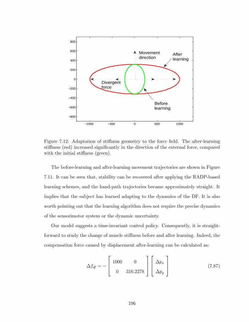
−1000 −500 0 500 1000
−800
−600
−400
−200
0
200
400
600
800
Movementdirection
Beforelearning
Divergentforce
Afterlearning
Figure 7.12: Adaptation of stiffness geometry to the force field. The after-learningstiffness (red) increased significantly in the direction of the external force, comparedwith the initial stiffness (green).
The before-learning and after-learning movement trajectories are shown in Figure
7.11. It can be seen that, stability can be recovered after applying the RADP-based
learning schemes, and the hand-path trajectories became approximately straight. It
implies that the subject has learned adapting to the dynamics of the DF. It is also
worth pointing out that the learning algorithm does not require the precise dynamics
of the sensorimotor system or the dynamic uncertainty.
Our model suggests a time-invariant control policy. Consequently, it is straight-
forward to study the change of muscle stiffness before and after learning. Indeed, the
compensation force caused by displacement after-learning can be calculated as:
∆fdf = −
1000 0
0 316.2278
∆px
∆py
(7.87)
196

In contrast, before the learning starts, the compensation force was
∆fnf = −
223.6068 0
0 316.2278
∆px
∆py
(7.88)
Now, the stiffness, defined as a graphical depiction of the elastic restoring force
corresponding to the unit displacement of the hand for the subject in the force fields
[22, 41], can be numerically computed. In addition, it can be presented in terms of an
ellipse by plotting the elastic force produced by a unit displacement [123]. In Figure
7.12, we plotted the stiffness ellipses. It can be seen that the difference between the
stiffness ellipses before and after learning is a direct result from the changes in both
the weighting matrices and the system dynamics.
7.4.2 Velocity-dependent force field with time delay
Now, we use the proposed RADP method to simulate the experiment conducted by
[142]. We model the velocity-dependent force field using the following dynamic system
d
fx
fy
= −
τf 0
0 τf
−1
×
fx
fy
−
−10.1 −11.2
−11.2 11.1
vx
vy
dt (7.89)
In the experiment [142], each subject was asked to move a cursor from the center of
a workspace to a target at an angle randomly chosen from the set 0, 45, · · · , 315,
and at a distance of 0.1m. After one target was reached, the next target, randomly
selected, was presented.
There were four different stages in the experiment. First, the subject made arm
movements without the force field. Second, the force field was applied without no-
tifying the subject. Third, the subject adapted to the force field. Finally, the force
field was suddenly removed and the after-learning effects were observed.
197
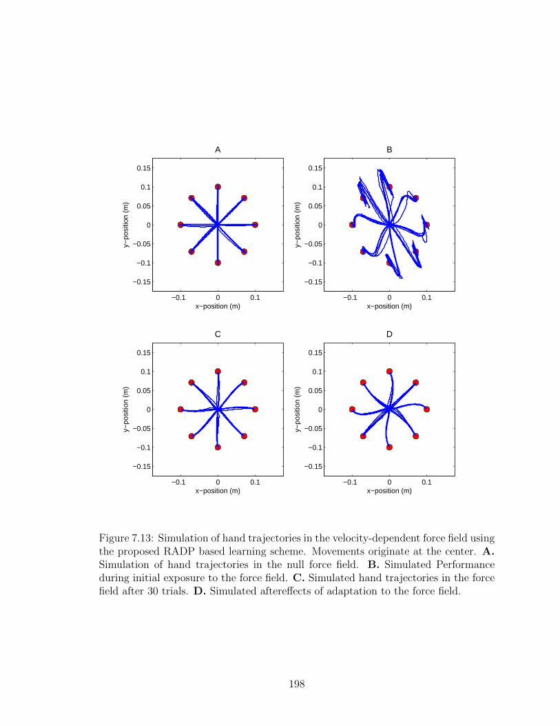
−0.1 0 0.1
−0.15
−0.1
−0.05
0
0.05
0.1
0.15
x−position (m)
y−po
sitio
n (m
)
A
−0.1 0 0.1
−0.15
−0.1
−0.05
0
0.05
0.1
0.15
x−position (m)y−
posi
tion
(m)
B
−0.1 0 0.1
−0.15
−0.1
−0.05
0
0.05
0.1
0.15
x−position (m)
y−po
sitio
n (m
)
C
−0.1 0 0.1
−0.15
−0.1
−0.05
0
0.05
0.1
0.15
x−position (m)
y−po
sitio
n (m
)
D
Figure 7.13: Simulation of hand trajectories in the velocity-dependent force field usingthe proposed RADP based learning scheme. Movements originate at the center. A.Simulation of hand trajectories in the null force field. B. Simulated Performanceduring initial exposure to the force field. C. Simulated hand trajectories in the forcefield after 30 trials. D. Simulated aftereffects of adaptation to the force field.
198
Before the force field was activated, the initial control policy we assumed was
the same as the one in the previous simulation. Once the CNS noticed the velocity-
dependent field, the new weighting matrices was replaced by
Q1 =
104 0 0 0
0 1000 0 0
0 0 1 0
0 0 0 1
, Q2 = I2,
R1 = R2 =
0.1 0
0 0.1
. (7.90)
The movement performance in the four different stages were simulated using the
proposed RADP algorithm and the results are given in Figure 7.13. In addition, we
plotted the velocity curves of the arm movement during the first three stages as shown
in Figure. Interestingly, consistency can be found by comparing Figure 7.14 in this
paper with Figure 10 in [142].
7.5 Discussion
7.5.1 Non-model-based learning
Most of the previous models for sensorimotor control have concluded that the CNS
knows precisely the knowledge of the motor system and its interacting environment
[33, 40, 50, 77, 131, 140, 163, 162, 165]. The computation of optimal control laws is
based on this assumption. By contrast, the proposed ADP methodology is a non-
model-based approach and informs that the optimal control policy is derived using
the real-time sensory data and is robust to dynamic uncertainties such as signal-
dependent noise. In the absence of external disturbances, our model can generate
199
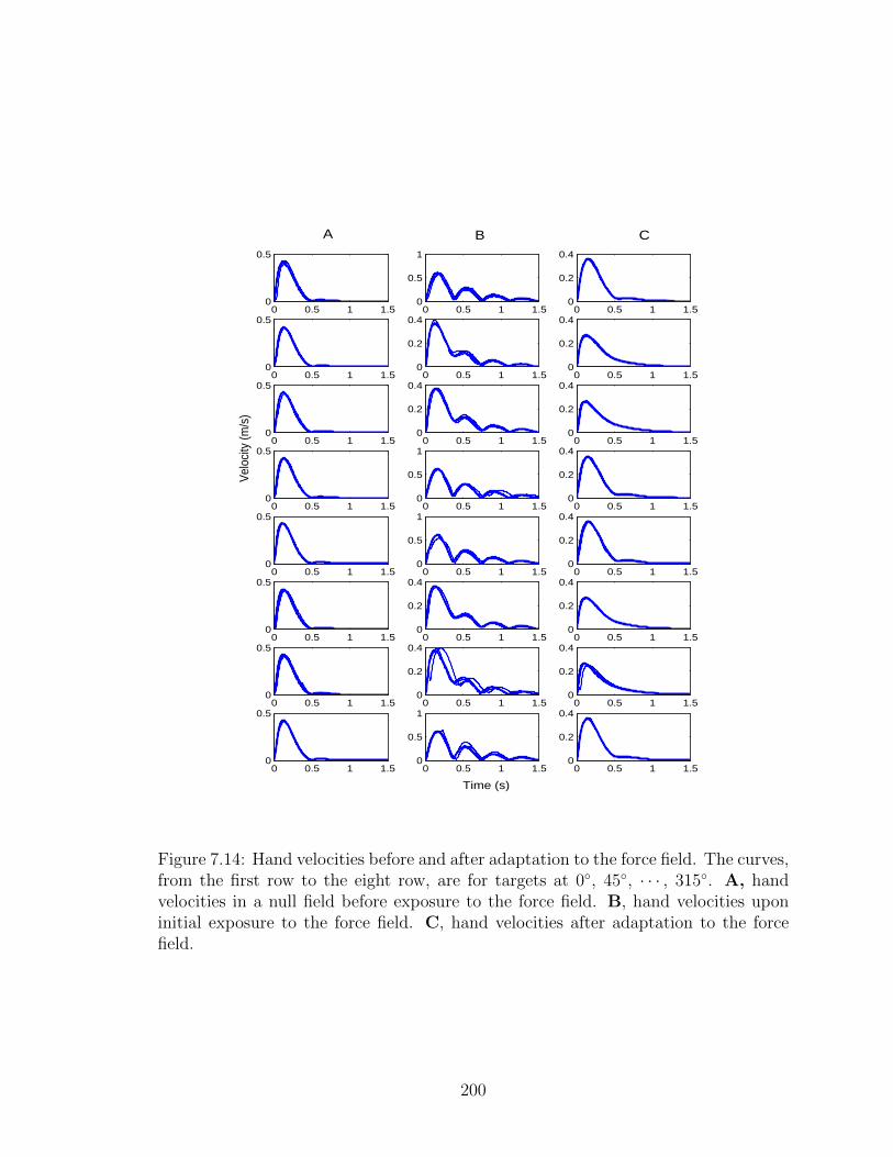
0 0.5 1 1.50
0.5
1
0 0.5 1 1.50
0.2
0.4
0 0.5 1 1.50
0.5V
eloc
ity (m
/s)
0 0.5 1 1.50
0.5
0 0.5 1 1.50
0.5
0 0.5 1 1.50
0.5
0 0.5 1 1.50
0.5
0 0.5 1 1.50
0.5
0 0.5 1 1.50
0.5
0 0.5 1 1.50
0.5
0 0.5 1 1.50
0.5
1
0 0.5 1 1.50
0.2
0.4
0 0.5 1 1.50
0.2
0.4
0 0.5 1 1.50
0.2
0.4
0 0.5 1 1.50
0.2
0.4
0 0.5 1 1.50
0.5
1
0 0.5 1 1.50
0.5
1
0 0.5 1 1.50
0.2
0.4
0 0.5 1 1.50
0.2
0.4
0 0.5 1 1.50
0.2
0.4
0 0.5 1 1.50
0.2
0.4
0 0.5 1 1.50
0.2
0.4
0 0.5 1 1.50
0.2
0.4
0 0.5 1 1.50
0.2
0.4
A B C
Time (s)
Figure 7.14: Hand velocities before and after adaptation to the force field. The curves,from the first row to the eight row, are for targets at 0, 45, · · · , 315. A, handvelocities in a null field before exposure to the force field. B, hand velocities uponinitial exposure to the force field. C, hand velocities after adaptation to the forcefield.
200
typically observed position, velocity, and endpoint force curves as produced by the
previous models. As one of the key differences with existing sensorimotor models, our
proposed computational mechanism suggests that, when confronted with unknown en-
vironments and imprecise dynamics, the CNS may update and improve its command
signals for movement through learning and repeated trials.
In the presence of perturbations, most of the previous models have relied on sen-
sory prediction errors to form an estimate of the perturbation [9, 92, 195]. However,
this viewpoint is difficult to be justified theoretically and has not been convincingly
validated by experiments. Indeed, evidence against this source-identified adaptation
is reported by [59], where a self-generated perturbation was created but it was not
identified or used in formulating the control policy. This is consistent with the learn-
ing scheme we proposed in this paper. Indeed, our ADP-based learning scheme does
not identify the dynamics of the force fields. Instead, optimal control policies in
the presence of force fields are directly obtained through successive approximations.
By simulating the experiments conducted by [22] and [41], we have found that our
computational results match well with the experimental results. In particular, our
simulation results show gradual adaptation to the unknown force fields, with nearly
identical movement trajectories in the first several consecutive trials reported in the
experiment [41]. The simulated post-learning velocity and endpoint force curves fit
well with the experimental observations [22, 41]. Our simulations clearly demonstrat-
ed the after-effects phenomenon.
7.5.2 Stability and convergence properties
Several reinforcement-learning-based models for motor adaptation have been devel-
oped in the past literature [35, 64]. However, it is not easy to analyze the convergence
and the stability properties of the learning schemes. In this paper, we have extended
the ADP theory to continuous-time linear systems with signal-dependent noise, and
201
applied this theory to model sensorimotor control. An added value of the proposed
ADP methodology is that rigorous convergence and stability analysis is given and is
surprisingly simple by means of linear optimal control theory.
7.5.3 Muscle stiffness
Several practical methods for experimentally measuring stiffness have been proposed
in the past literature [21, 47, 54], and the changes of stiffness in force fields were
reported by [22] and [41]. However, how the CNS modifies the stiffness geometry
and achieves optimal motor behavior remains a largely open question. [22] suggested
that the CNS minimizes the hand-path error relative to a straight line joining the
start position and the target center. This optimization problem does not involve any
system dynamics, and cannot link the modification of stiffness to optimal feedback
control theory. On the other hand, the stiffness may not be well analyzed using other
models based on finite-horizon optimal control theory (see, for example, [162, 50]).
This is because those models use time-varying control policies, leading to continuous
change of the stiffness during the movement.
In the ADP-based model, time-invariant control policies are computed, and it is
comparably easy to analyze the muscle stiffness by studying the position feedback
gains. Our modeling methodology implies that the change of stiffness results from
the modification of the weighing matrices by the CNS and the change of the system
dynamics. Indeed, our simulation results provide similar stiffness ellipses as those
measured in experiments [22, 41]. In addition, our model suggests that different stiff-
ness geometries of different individuals may be a consequence of different weighting
matrices they selected. Therefore, compared with other models of motor control and
motor adaptation, our modeling strategy can explain naturally the change of stiffness
observed in experiments from the viewpoint of optimal feedback control [99].
202
7.5.4 Data fitting for the weighting matrices
The weighting matrices we used in the numerical simulation are selected such that our
resultant computational results can have qualitative consistency with experimental
results [22, 41]. If accurate human motor data become available, better fits for the
weights can be obtained using a two-loop optimization approach [65]. The inner-loop
uses the proposed ADP method to approximate an optimal control policy and gen-
erate the stiffness ellipses. The outer-loop compares the error between the simulated
stiffness ellipses with experimental observations and adjusts the parameters qx, qy,
and θ to minimize the error.
7.5.5 Infinite-horizon optimal control
During each trial, a time-invariant control policy is suggested in our methodology.
The time-invariant control policy has a main advantage that movement duration does
not need to be pre-fixed by the CNS. This seems more realistic because the duration
of each movement is different from each other due to the signal-dependent noise and
is difficult to be pre-fixed. [163] suggested that if the target is not reached at the
predicted reaching time, the CNS can similarly plan an independent new trajectory
between the actual position of the hand and the final target, and the final trajectory
will be the superposition of all the trajectories. By contrast, our model matches the
intuitive notion that the motor system keeps moving the hand toward the target until
it is reached, and much less computational burden is required. Our simulation results
match well with Fitts’s law predictions. In addition, this type of control policies can
also be used to analytically derive the Fitts’s law as illustrated by [131].
203
7.5.6 Comparison with iterative learning control
Iterative learning control (ILC) is an open-loop control scheme that iteratively learns
a feedforward signal based on the tracking error of the previous trials [20]. It has
also been used to model motor learning [208]. Compared with ILC, the ADP-based
learning method has at least three advantages. First, conventional ILC method uses
open-loop control policy for each individual trial. Hence, it may not explain the feed-
back control mechanism involved in each individual movement, which is essential in
generating bell-shaped velocity-curves. Second, ILC assumes the external disturbance
is iteration invariant. However, motor uncertainties do not satisfy this assumption,
since no two movements are exactly the same. Third, in the ILC model, learning only
happens among different trials. Therefore, it cannot model the online learning during
a single trial. On the other hand, this online learning process can be modeled by our
ADP method, since the ADP scheme gives the flexibility to specify the amount of
time that is needed for collecting online data and updating the control policy. Indeed,
if the time duration is set to be less than the time needed for one trial, then online
learning during one movement can be simulated.
7.5.7 Connection between optimality and robustness
Although optimal control theory is the dominant paradigm for understanding motor
behavior, and optimization based models can explain many aspects of sensor motor
control, it is not clear if the CNS keeps using the optimal control policy when dynamic
uncertainty occurs. Experimental results obtained by [59] show that the control
scheme employed by the CNS in the presence of external disturbances may only be
sub-optimal because the control scheme they observed experimentally is not energy
efficient. Indeed, in the presence of dynamic uncertainties, guaranteeing optimality
and stability becomes a nontrivial task.
The RADP studies the stability of interconnected systems by analyzing the gain
204
conditions (7.32), (7.33), and (7.42)-(7.44), which are inspired by a simplified version
of the nonlinear small-gain theorem [83]. As shown previously, these conditions can
be satisfied by choosing suitable cost functions with appropriately designed weighting
matrices [69]. It should be mentioned that the control policy generated from our
RADP method is optimal for the nominal/reduced system, and remains stable and
retains suboptimality in the presence of dynamic uncertainty. The change of stiffness
in the divergent force field was reported by [22]. However, they assumed that the
stiffness was modified to minimize some cost function associated with the minimum-
jerk model [40] which does not involve optimal feedback control theory. Alternatively,
in the RADP theory, the change of stiffness can be interpreted as a direct result of
the change of weighting matrices.
Hence, the proposed RADP theory is compatible with the optimal control theory
and the experimental results observed in the past literature. More importantly, it
provides a unified framework that naturally connects optimality and robustness to
explain the motor behavior with/without uncertainties.
7.6 Conclusions
We have developed ADP and RADP methods for linear stochastic systems with signal-
dependent noise with an objective to model goal-oriented sensorimotor control sys-
tems. An appealing feature of this new computational mechanism of sensorimotor
control is that the CNS does not rely upon the a priori knowledge of systems dynamics
and the environment to generate a command signal for hand movement. Our theory
can explain the change of stiffness geometry from a perspective of adaptive optimal
feedback control versus nonadaptive optimal control theory [131, 163, 162]. In par-
ticular, the RADP theory not only gives computational results which are compatible
with experimental data [22, 41, 142], but also provides a unified framework to study
205

robustness and optimality simultaneously. We therefore argue that the human motor
system may use ADP and RADP-like mechanisms to control movements.
206
Chapter 8
Conclusions and future work
8.1 Conclusions
This dissertation has proposed our recent contributions to the new framework of
RADP and illustrated its potential applications. The major contributions of this
dissertation can be summarized from two aspects.
On one hand, developing ADP-based methodology for the continuous-time (CT)
setting with completely unknown dynamics is a challenging topic. Indeed, although
the action-dependent heuristic dynamic programming [189] (or Q-learning [181]) does
not depend on the discrete-time (DT) system, it cannot be directly applied for solving
CT problems, such as the problems addressed in this dissertation. One major reason is
that the structures of CT algebraic Riccati equations (AREs) or the Hamilton-Jacobi-
Bellman (HJB) equations are significantly different from their DT counterparts. This
dissertation has introduced a novel computational policy iteration approach we devel-
oped recently [68]. It finds online adaptive optimal controllers for CT linear systems
with completely unknown system dynamics, and solves the ARE iteratively using
system state and input information collected online, without knowing the system ma-
trices. This objective is achieved by taking advantages of the exploration noise. This
207

methodology has been further extended for affine nonlinear systems. An immediate
result has been obtained by using neural networks (NNs) to approximate online the
cost function and the new control policy [75]. We have provided rigorous proofs on
the convergence property of this method. However, NNs-based approximation can
only be effective on some compact set, and it is generally not trivial to determine the
type of basis functions to achieve good approximation performance. Therefore, we
have proposed for the first time the idea of global adaptive dynamic programming
(GADP), which finds a suboptimal control policy but provides global stability and
gives rise to computational efficiency.
On the other hand, in the past literature of ADP, it is commonly assumed that
both the system order is known and the state variables are perfectly measurable.
These two conditions are generally restrictive and are needed to be relaxed in further
research. In addition, it is widely recognized that, besides maximizing the reward
from the environment, biological systems learn to achieve enhanced robustness (or
greater chance of survival) through interacting with the unknown environment, and
they may only be able to make decisions based on partial-state information due to
the complexity of the real-world environment. This dissertation bridges the gap in
the past literature of ADP where dynamic uncertainties or unmodeled dynamics were
not addressed. In this dissertation, two strategies have been introduced to achieve
robust stabilization in the presence of dynamic uncertainties. First, for partially
linear systems [75] and weakly nonlinear large-scale systems [70], we have derived
conditions on the weighting matrices for the performance indices for each nominal
system. These conditions are in spirit of the small-gain theorem [83]. Second, for
affine nonlinear systems which interact with nonlinear dynamic uncertainties, we have
employed the robust redesign technique [83, 129] and the Lyapunov-based small-gain
theorem [81]. This methodology has been used to redesign the approximate optimal
control policy obtained using the NN-based approximation to achieve robust optimal
208
stabilization [75]. Also, it has been employed to redesign the suboptimal control
policy obtained using the SOS-based policy iteration, such that global robust and
suboptimal stabilization can be achieved [71].
We have applied the proposed online learning methodologies for engineering appli-
cations. In particular, the RADP method finds good applications in power systems
related control problems. Simulations for a two-machine and a ten-machine pow-
er systems have been been provided to show the efficiency and effectiveness of the
proposed algorithms. Further, since RADP shares many essential features with rein-
forcement learning, we found it is reasonable to use RADP as a reverse-engineering
approach to model human motor control and learning. To this end, we have developed
RADP-based learning methods to study stochastic systems with control-dependent
noise, and use these methods to numerically reproduce experimental results obtained
in [22, 41, 142]. Observing the strong consistency of numerical results with experi-
mental data, we argue that the central nervous system (CNS) may use RADP-like
mechanisms to coordinate movements in the presence of static and/or dynamic un-
certainties.
8.2 Future work
A gap has been bridged by the development of the RADP framework, in which dy-
namic uncertainty is taken into account. However, compared with a true brain-like
intelligent learning control system, results presented in this dissertation are only the
tips of an iceberg. Quite a few interesting and exciting related topics deserve further
research. For example, the following are some of the directions for continuation of
this work.
1. Extending the current results on GADP for more generalized nonlinear systems,
such as nonaffine nonlinear systems [14].
209
2. Gaining more insights into understanding the rank condition and its relations
with the exploration noise.
3. Developing output-feedback-based RADP theory (see [46] for some preliminary
results).
4. Extending the current ADP and RADP methodologies for nonlinear stochas-
tic systems, and apply them to more realistic models to study human motor
learning (see [14, 15] for some preliminary results ).
5. Enriching the features of ADP and RADP theories by incorporating more
biologically-inspired learning behaviors.
6. Developing RADP-based tracking methods to achieve online tracking with both
static and dynamic uncertainties.
7. Quantifying the sub-optimality in the presence of dynamic uncertainties.
Finally, the author believes that the RADP theory developed in this thesis has nu-
merous potential applications in practical engineering systems and reverse-engineering
problems. In addition to further developing and refining the theory of RADP, it is also
important to study the practical implementation issues for real-world applications.
210
Chapter 9
Appendices
9.1 Review of optimal control theory
9.1.1 Linear quadratic regulator (LQR) for CT linear sys-
tems
Consider a CT linear system described by
x = Ax+Bu (9.1)
where x ∈ Rn is the system state fully available for feedback control design; u ∈ Rm
is the control input; A ∈ Rn×n and B ∈ Rn×m are unknown constant matrices. In
addition, the system is assumed to be stabilizable.
The design objective is to find a linear optimal control law in the form of
u = −Kx (9.2)
211
which minimizes the following performance index
J =
∫ ∞
0
(xTQx+ uTRu)dt, x(0) = x0 ∈ Rn, (9.3)
where Q = QT ≥ 0, R = RT > 0, with (A,Q1/2) observable.
By linear optimal control theory [103], when both A and B are accurately known,
solution to this problem can be found by solving the following well-known algebraic
Riccati equation (ARE)
ATP + PA+Q− PBR−1BTP = 0. (9.4)
If the pair (A,B) is stabilizable and the pair (A,Q1/2) is observable, (9.4) has a
unique symmetric positive definite solution P ∗. The optimal feedback gain matrix
K∗ in (9.2) can thus be determined by
K∗ = R−1BTP ∗. (9.5)
Notice that the optimal feedback gain matrix K∗ does not depend on the initial
condition x0.
9.1.2 Nonlinear optimal control for CT affine nonlinear sys-
tems
Consider the nonlinear system
x = f(x) + g(x)u (9.6)
where x ∈ Rn is the system state, u ∈ Rm is the control input, f(x) and g(x) are
locally Lipschitz functions with f(0) = 0.
212
In classical nonlinear optimal control theory [103], the common objective is to find
a control policy u that minimizes certain performance, which takes, for example, the
following form.
J(x0, u) =
∫ ∞
0
r(x(t), u(t))dt, x(0) = x0 (9.7)
where r(x, u) = Q(x) + uTRu, with Q(x) a positive definite function, and R is a
symmetric positive definite matrix. Notice that, the purpose of specifying r(x, u) in
this form is to guarantee that an optimal control policy can be explicitly determined,
if it exists.
Now, suppose there exists V o ∈ P , such that the Hamilton-Jacobi-Bellman (HJB)
equation holds
H(V o) = 0 (9.8)
where
H(V ) = ∇V T (x)f(x) +Q(x)− 1
4∇V T (x)g(x)R−1gT (x)∇V (x).
Then, it is easy to see that V o is a well-defined Lyapunov function for the closed-
loop system comprised of (9.6) and
uo(x) = −1
2R−1gT (x)∇V o(x). (9.9)
Hence, this closed-loop system is globally asymptotically stable at x = 0 [86].
Then, according to [141, Theorem 3.19], uo is the optimal control policy, and the
value function V o(x0) gives the optimal cost at the initial condition x(0) = x0, i.e.,
V o(x0) = minuJ(x0, u) = J(x0, u
o), ∀x0 ∈ Rn. (9.10)
213
It can also be shown that V o is the unique solution to the HJB equation (9.8)
with V o ∈ P . Indeed, let V ∈ P be another solution to (9.8). Then, by Theorem
3.19 in [141], along the solutions of the closed-loop system composed of (9.6) and
u = u = −12R−1gT∇V , it follows that
V (x0) = V o(x0)−∫ ∞
0
|uo − u|2Rdt, ∀x0 ∈ Rn. (9.11)
Finally, comparing (9.10) and (9.11), we conclude that V o = V .
9.2 Review of ISS and the nonlinear small-gain
theorem
Here we review some important tools from modern nonlinear control; see, for instance,
[61, 83, 80, 86, 114, 150], and references therein for the details. See [85] for more recent
developments in nonlinear systems and control.
Consider the system
x = f(x, u) (9.12)
where x ∈ Rn is the state, u ∈ Rm is the input, and f : Rn × Rm → Rn is locally
Lipschitz.
Definition 9.2.1 ([148, 149]). The system (9.12) is said to be input-to-state stable
(ISS) with gain γ if, for any measurable essentially bounded input u and any initial
condition x(0), the solution x(t) exists for every t ≥ 0 and satisfies
|x(t)| ≤ β(|x(0)|, t) + γ(‖u‖) (9.13)
where β is of class KL and γ is of class K.
214
Definition 9.2.2 ([151]). A continuously differentiable function V is said to be an
ISS-Lyapunov function for the system (9.12) if V is positive definite and proper, and
satisfies the following implication:
|x| ≥ χ(|u|)⇒ ∇V (x)Tf(x, u) ≤ −κ(|x|) (9.14)
where κ is positive definite and χ is of class K.
Next, consider an interconnected system described by
x1 = f1(x1, x2, v), (9.15)
x2 = f2(x1, x2, v) (9.16)
where, for i = 1, 2, xi ∈ Rni , v ∈ Rnv , fi : Rn1 ×Rn2 ×Rnv → Rni is locally Lipschitz.
Assumption 9.2.1. For each i = 1, 2, there exists an ISS-Lyapunov function Vi for
the xi subsystem such that the following hold:
1. there exist functions αi, αi ∈ K∞, such that
αi(|xi|) ≤ Vi(xi) ≤ αi(|xi|), ∀xi ∈ Rni ; (9.17)
2. there exist class K functions χi, γi and a class K∞ function αi, such that
∇V1(x1)Tf1(x1, x2, v) ≤ −α1(V1(x1)), (9.18)
if V1(x1) ≥ maxχ1(V2(x2)), γ1(|v|), and
∇V2(x2)Tf2(x1, x2, v) ≤ −α2(V2(x2)), (9.19)
if V2(x2) ≥ maxχ2(V1(x1)), γ2(|v|).
215
Based on the ISS-Lyapunov functions, the following theorem gives the small-gain
condition, under which the ISS property of the interconnected system can be achieved.
Theorem 9.2.1 ([81]). Under Assumption 9.2.1, if the following small-gain condition
holds:
χ1 χ2(s) < s, ∀s > 0, (9.20)
then, the interconnected system (9.15), (9.16) is ISS with respect to v as the input.
Under Assumption 9.2.1 and the small-gain condition (9.20), Let χ1 be a function
of class K∞ such that
1. χ1(s) ≤ χ−11 (s), ∀s ∈ [0, lim
s→∞χ1(s)),
2. χ2(s) ≤ χ1(s), ∀s ≥ 0.
Then, as shown in [81], there exists a class K∞ function σ(s) which is continuously
differentiable over (0,∞) and satisfies dσds
(s) > 0 and χ2(s) < σ(s) < χ1(s), ∀s > 0.
In [81], it is also shown that the function
V12(x1, x2) = maxσ(V1(x1)), V2(x2) (9.21)
is positive definite and proper. In addition, we have
V12(x1, x2) < 0 (9.22)
holds almost everywhere in the state space, whenever
V12(x1, x2) ≥ η(|v|) > 0 (9.23)
for some class K∞ function η.
216
9.3 Matlab code for the simulation in Chapter 2
For the readers’ convenience, here I put the MATLAB code for the very first simu-
lation in the dissertation. All the other simulations can be made using the same
techniques. A few other available MATLAB programs can be found on the au-
thor’s personal website at http://files.nyu.edu/yj348/public/index.html. They are
also available upon request.
% Code for the paper "Computational adaptive optimal control with an
% application to a car engine control problem", Yu Jiang and Zhong-Ping
% Jiang,vol. 48, no. 10, pp. 2699-2704, Oct. 2012.
% \copyright Copyright 2011-2014 Yu Jiang, New York University.
function []=engine_main()
clc;
x_save=[];
t_save=[];
flag=1; % 1: learning is on. 0: learning is off.
% System matrices used for simulation purpose
A=[-0.4125 -0.0248 0.0741 0.0089 0 0;
101.5873 -7.2651 2.7608 2.8068 0 0;
0.0704 0.0085 -0.0741 -0.0089 0 0.0200;
0.0878 0.2672 0 -0.3674 0.0044 0.3962;
-1.8414 0.0990 0 0 -0.0343 -0.0330;
0 0 0 -359 187.5364 -87.0316];
B=[-0.0042 0.0064
-1.0360 1.5849
0.0042 0;
0.1261 0;
0 -0.0168;
0 0];
[xn,un]=size(B);%size of B. un-column #, xn row #
% Set the weighting matrices for the cost function
Q=diag([1 1 0.1 0.1 0.1 0.1]);
R=eye(2);
217
% Initialize the feedback gain matrix
K=zeros(un,xn); % Only if A is Hurwitz, K can be set as zero.
N=200; %Length of the window, should be at least greater than xn^2
NN=10; %Max iteration times
T=.01; %Duration of time for each integration
%x0=[10;2;100;2;-1;-2]; %Initial condition
x0=[10;2;10;2;-1;-2];
i1=(rand(1,100)-.5)*1000;
i2=(rand(1,100)-.5)*1000;
Dxx=[];XX=[];XU=[]; % Data matrices
X=[x0;kron(x0’,x0’)’;kron(x0,zeros(un,1))]’;
% Run the simulation and obtain the data matrices \delta_xx, I_xx,
% and I_xu
for i=1:N
% Simulation the system and at the same time collect online info.
[t,X]=ode45(@mysys, [(i-1)*T,i*T],X(end,:));
%Append new data to the data matrices
Dxx=[Dxx;kron(X(end,1:xn),X(end,1:xn))-kron(X(1,1:xn),X(1,1:xn))];
XX=[XX;X(end,xn+1:xn+xn^2)-X(1,xn+1:xn+xn^2)];
XU=[XU;X(end,xn+xn^2+1:end)-X(1,xn+xn^2+1:end)];
% Keep track of the system trajectories
x_save=[x_save;X];
t_save=[t_save;t];
end
Dxx=processing_Dxx(Dxx); % Only the distinct columns left
% K=zeros(un,xn); % Initial stabilizing feedback gain matrix
P_old=zeros(xn);P=eye(xn)*10; % Initialize the previous cost matrix
it=0; % Counter for iterations
p_save=[]; % Track the cost matrices in all the iterations
k_save=[]; % Track the feedback gain matrix in each iterations
[K0,P0]=lqr(A,B,Q,R) % Calculate the ideal solution for comparion purpose
k_save=[norm(K-K0)];
while norm(P-P_old)>1e-10 & it<16 % Stopping criterion for learning
it=it+1 % Update and display the # of iters
218
P_old=P; % Update the previous cost matrix
QK=Q+K’*R*K; % Update the Qk matrix
X2=XX*kron(eye(xn),K’); %
X1=[Dxx,-X2-XU]; % Left-hand side of the key equation
Y=-XX*QK(:); % Right-hand side of the key equation
pp=X1\Y; % Solve the equations in the LS sense
P=reshape_p(pp); % Reconstruct the symmetric matrix
p_save=[p_save,norm(P-P0)]; % Keep track of the cost matrix
BPv=pp(end-(xn*un-1):end);
K=inv(R)*reshape(BPv,un,xn)/2 % Get the improved gain matrix
k_save=[k_save,norm(K-K0)]; % Keep track of the control gains
end
% Plot the trajectories
figure(1)
plot([0:length(p_save)-1],p_save,’o’,[0:length(p_save)-1],p_save)
axis([-0.5,it-.5,-5,15])
legend(’||P_k-P^*||’)
xlabel(’Number of iterations’)
figure(2)
plot([0:length(k_save)-1],k_save,’^’,[0:length(k_save)-1],k_save)
axis([-0.5,it+0.5,-.5,2])
legend(’||K_k-K^*||’)
xlabel(’Number of iterations’)
% Post-learning simulation
[tt,xx]=ode23(@mysys,[t(end) 200],X(end,:)’);
% Keep track of the post-learning trajectories
t_final=[t_save;tt];
x_final=[x_save;xx];
figure(3)
plot(t_final,x_final(:,1:6),’Linewidth’,2)
axis([0,10,-100,200])
legend(’x_1’,’x_2’,’x_3’,’x_4’,’x_5’,’x_6’)
xlabel(’Time (sec)’)
figure(4)
plot(t_final,sqrt(sum(x_final(:,1:6).^2,2)),’Linewidth’,2)
axis([0,200,-50,200])
219

legend(’||x||’)
xlabel(’Time (sec)’)
figure(5)
plot(t_final,3.6*x_final(:,1),’k-.’, ...
t_final, x_final(:,6),’-’,’Linewidth’,2)
axis([0,10,-80,50])
legend(’y_1 (MAF)’,’y_2 (MAP)’)
xlabel(’Time (sec)’)
% The following nested function gives the dynamics of the sytem. Also,
% integraters are included for the purpose of data collection.
function dX=mysys(t,X)
%global A B xn un i1 i2 K flag
x=X(1:xn);
if t>=2; % See if learning is stopped
flag=0;
end
if flag==1
u=zeros(un,1);
for i=i1
u(1)=u(1)+sin(i*t)/length(i1); % constructing the
% exploration noise
end
for i=i2
u(2)=u(2)+sin(i*t)/length(i2);
end
u=10000*u;
else
u=-K*x;
end
dx=A*x+B*u;
dxx=kron(x’,x’)’;
dux=kron(x’,u’)’;
dX=[dx;dxx;dux];
end
% This nested function reconstruct the P matrix from its distinct elements
function P=reshape_p(p)
P=zeros(xn);
ij=0;
for i=1:xn
220
for j=1:i
ij=ij+1;
P(i,j)=p(ij);
P(j,i)=P(i,j);
end
end
end
% The following nested function removes the repeated columns from Dxx
function Dxx=processing_Dxx(Dxx)
ij=[]; ii=[];
for i=1:xn
ii=[ii (i-1)*xn+i];
end
for i=1:xn-1
for j=i+1:xn
ij=[ij (i-1)*xn+j];
end
end
Dxx(:,ii)=Dxx(:,ii)/2;
Dxx(:,ij)=[];
Dxx=Dxx*2;
end
end
221
Bibliography
[1] A. Al-Tamimi, F. L. Lewis, and M. Abu-Khalaf. Model-free Q-learning designsfor linear discrete-time zero-sum games with application to h-infinity control.Automatica, 43(3):473–481, 2007.
[2] A. Al-Tamimi, F. L. Lewis, and M. Abu-Khalaf. Discrete-time nonlinearHJB solution using approximate dynamic programming: convergence proof.IEEE Transactions on Systems, Man, and Cybernetics, Part B: Cybernetics,38(4):943–949, 2008.
[3] D. Angeli and E. D. Sontag. Forward completeness, unboundedness observabili-ty, and their Lyapunov characterizations. Systems & Control Letters, 38(4):209–217, 1999.
[4] L. C. Baird. Reinforcement learning in continuous time: Advantage updating.In Proceedings of the IEEE World Congress on Computational Intelligence, vol-ume 4, pages 2448–2453, 1994.
[5] A. G. Barto, R. S. Sutton, and C. W. Anderson. Neuronlike adaptive elementsthat can solve difficult learning control problems. IEEE Transactions on Sys-tems, Man and Cybernetics, 13(5):834–846, 1983.
[6] R. W. Beard, G. N. Saridis, and J. T. Wen. Galerkin approximations of thegeneralized Hamilton-Jacobi-Bellman equation. Automatica, 33(12):2159–2177,1997.
[7] R. Bellman and S. Dreyfus. Functional approximations and dynamic program-ming. Mathematical Tables and Other Aids to Computation, 13(68):247–251,1959.
[8] R. E. Bellman. Dynamic Programming. Princeton University Press, Princeton,NJ, 1957.
[9] M. Berniker and K. Kording. Estimating the sources of motor errors for adap-tation and generalization. Nature Neuroscience, 11(12):1454–1461, 2008.
[10] D. P. Bertsekas. Dynamic Programming and Optimal Control, 4th ed. AthenaScientific Belmont, Belmonth, MA, 2007.
222
[11] D. P. Bertsekas and J. N. Tsitsiklis. Neuro-Dynamic Programming. AthenaScientific, Nashua, NH, 1996.
[12] S. Bhasin, N. Sharma, P. Patre, and W. Dixon. Asymptotic tracking by a rein-forcement learning-based adaptive critic controller. Journal of Control Theoryand Applications, 9(3):400–409, 2011.
[13] N. Bhushan and R. Shadmehr. Computational nature of human adaptive controlduring learning of reaching movements in force fields. Biological Cybernetics,81(1):39–60, 1999.
[14] T. Bian, Y. Jiang, and Z. P. Jiang. Adaptive dynamic programming and optimalcontrol of nonlinear nonaffine systems. Automatica, provisionally accepted, 2014.
[15] T. Bian, Y. Jiang, and Z. P. Jiang. Adaptive dynamic programming for s-tochastic systems with state and control dependent noise. IEEE Transactionson Automatic Control, submitted, 2014.
[16] T. Bian, Y. Jiang, and Z. P. Jiang. Decentralized and adaptive optimal controlof large-scale systems with application to power systems. IEEE Transactionson Industrial Electronics, revised, Apr 2014.
[17] G. Blekherman, P. A. Parrilo, and R. R. Thomas, editors. Semidefinite Opti-mization and Convex Algebraic Geometry. SIAM, Philadelphia, PA, 2013.
[18] V. S. Borkar. Stochastic approximation: a dynamical systems viewpoint. Cam-bridge University Press Cambridge, 2008.
[19] S. J. Bradtke, B. E. Ydstie, and A. G. Barto. Adaptive linear quadratic controlusing policy iteration. In Proceedings of the American Control Conference,volume 3, pages 3475–3479. IEEE, 1994.
[20] D. A. Bristow, M. Tharayil, and A. G. Alleyne. A survey of iterative learningcontrol. IEEE Control Systems Magazine, 26(3):96–114, 2006.
[21] E. Burdet, R. Osu, D. Franklin, T. Yoshioka, T. Milner, and M. Kawato. Amethod for measuring endpoint stiffness during multi-joint arm movements.Journal of Biomechanics, 33(12):1705–1709, 2000.
[22] E. Burdet, R. Osu, D. W. Franklin, T. E. Milner, and M. Kawato. The centralnervous system stabilizes unstable dynamics by learning optimal impedance.Nature, 414(6862):446–449, 2001.
[23] L. Busoniu, R. Babuska, B. De Schutter, and D. Ernst. Reinforcement learningand dynamic programming using function approximators. CRC Press, 2010.
[24] M. Chen. Some simple synchronization criteria for complex dynamical networks.IEEE Transactions on Circuits and Systems II: Express Briefs, 53(11):1185–1189, 2006.
223
[25] P.-C. Chen and M. Kezunovic. Analysis of the impact of distributed generationplacement on voltage profile in distribution systems. In Proceedings of the 2013IEEE Power and Energy Society General Meeting (PES), pages 1–5, Vancouver,BC, Jul 2013.
[26] P.-C. Chen, V. Malbasa, and M. Kezunovic. Analysis of voltage stability issueswith distributed generation penetration in distribution networks. In Proceed-ings of the 2013 IEEE North American Power Symposium (NAPS), pages 1–6,Manhattan, KS, 2013.
[27] P.-C. Chen, R. Salcedo, Q. Zhu, F. de Leon, D. Czarkowski, Z. P. Jiang, V. Spit-sa, Z. Zabar, and R. E. Uosef. Analysis of voltage profile problems due to thepenetration of distributed generation in low-voltage secondary distribution net-works. IEEE Transactions on Power Delivery, 27(4):2020–2028, 2012.
[28] Z. Chen and J. Huang. Global robust stabilization of cascaded polynomialsystems. Systems & Control Letters, 47(5):445–453, 2002.
[29] Z. Chen, L. Wu, and Y. Fu. Real-time price-based demand response manage-ment for residential appliances via stochastic optimization and robust optimiza-tion. IEEE Transactions on Smart Grid, 3(4):1822–1831, 2012.
[30] D. A. Cox. Ideals, Varieties, and Algorithms: An Introduction to ComputationalAlgebraic Geometry and Commutative Algebra. Springer, 2007.
[31] P. R. Davidson and D. M. Wolpert. Motor learning and prediction in a variableenvironment. Current Opinion in Neurobiology, 13(2):232–237, 2003.
[32] D. P. de Farias and B. Van Roy. The linear programming approach to approx-imate dynamic programming. Operations Research, 51(6):850–865, 2003.
[33] J. Diedrichsen, R. Shadmehr, and R. B. Ivry. The coordination of movement:optimal feedback control and beyond. Trends in Cognitive Sciences, 14(1):31–39, 2010.
[34] T. Dierks and S. Jagannathan. Output feedback control of a quadrotor uavusing neural networks. IEEE Transactions on Neural Networks, 21(1):50–66,2010.
[35] K. Doya. Reinforcement learning in continuous time and space. Neural Com-putation, 12(1):219–245, 2000.
[36] K. Doya, H. Kimura, and M. Kawato. Neural mechanisms of learning andcontrol. IEEE Control Systems Magazine, 21(4):42–54, 2001.
[37] P. D. Feldkamp LA. Recurrent neural networks for state estimation. In Pro-ceedings of the Twelve Yale Workshop on Adaptive and Learning Systems, pages17–22, New Haven, CT, 2003.
224
[38] S. Ferrari, J. E. Steck, and R. Chandramohan. Adaptive feedback control byconstrained approximate dynamic programming. Systems, Man, and Cybernet-ics, Part B: Cybernetics, IEEE Transactions on, 38(4):982–987, 2008.
[39] P. M. Fitts. The information capacity of the human motor system in controllingthe amplitude of movement. Journal of Experimental Psychology, 47(6):381–391, 1954.
[40] T. Flash and N. Hogan. The coordination of arm movements: an experimentallyconfirmed mathematical model. The Journal of Neuroscience, 5(7):1688–1703,1985.
[41] D. W. Franklin, E. Burdet, R. Osu, M. Kawato, and T. E. Milner. Functionalsignificance of stiffness in adaptation of multijoint arm movements to stable andunstable dynamics. Experimental Brain Research, 151(2):145–157, 2003.
[42] D. W. Franklin, E. Burdet, K. P. Tee, R. Osu, C.-M. Chew, T. E. Milner, andM. Kawato. CNS learns stable, accurate, and efficient movements using a simplealgorithm. The Journal of Neuroscience, 28(44):11165–11173, 2008.
[43] D. W. Franklin and D. M. Wolpert. Computational mechanisms of sensorimotorcontrol. Neuron, 72(3):425–442, 2011.
[44] G. Franze, D. Famularo, and A. Casavola. Constrained nonlinear polynomi-al time-delay systems: A sum-of-squares approach to estimate the domain ofattraction. IEEE Trans. Auto. Contr., 57(10):2673–2679, 2012.
[45] P. Gahinet, A. Nemirovskii, A. J. Laub, and M. Chilali. The LMI controltoolbox. In Proceedings of the 33rd IEEE Conference on Decision and Control,volume 3, pages 2038–2041, 1994.
[46] W. Gao, Y. Jiang, Z. P. Jiang, and T. Chai. Adaptive and optimal output feed-back control of linear systems: an adaptive dynamic programming approach.In The 11th World Congress on Intelligent Control and Automation, accepted,Shenyang, China, June 2014.
[47] H. Gomi and M. Kawato. Equilibrium-point control hypothesis examined bymeasured arm stiffness during multijoint movement. Science, 272:117–120, 1996.
[48] M. Grant and S. Boyd. Cvx: Matlab software for disciplined convex program-ming, version 2.0 beta. http://cvxr.com/cvx, 2013.
[49] G. Guo, Y. Wang, and D. J. Hill. Nonlinear output stabilization control formultimachine power systems. IEEE Transactions on Circuits and Systems I:Fundamental Theory and Applications, 47(1):46–53, 2000.
[50] C. M. Harris and D. M. Wolpert. Signal-dependent noise determines motorplanning. Nature, 394:780–784, 1998.
225
[51] H. He, Z. Ni, and J. Fu. A three-network architecture for on-line learningand optimization based on adaptive dynamic programming. Neurocomputing,78(1):3–13, 2012.
[52] J. W. Helton and M. R. James. Extending H∞ Control to Nonlinear Systems:Control of Nonlinear Systems to Achieve Performance Objectives. SIAM, 1999.
[53] D. Henrion and J.-B. Lasserre. Gloptipoly: Global optimization over polyno-mials with Matlab and SeDuMi. ACM Transactions on Mathematical Software,29(2):165–194, 2003.
[54] N. Hogan. The mechanics of multi-joint posture and movement control. Bio-logical Cybernetics, 52(5):315–331, 1985.
[55] N. Hogan and T. Flash. Moving gracefully: quantitative theories of motorcoordination. Trends in Neurosciences, 10(4):170–174, 1987.
[56] R. A. Horn and C. R. Johnson. Matrix analysis. Cambridge University Press,1990.
[57] K. Hornik, M. Stinchcombe, and H. White. Multilayer feedforward networksare universal approximators. Neural Networks, 2(5):359–366, 1989.
[58] R. Howard. Dynamic Programming and Markov Processes. MIT Press, Cam-bridge, MA, 1960.
[59] T. E. Hudson and M. S. Landy. Adaptation to sensory–motor reflex perturba-tions is blind to the source of errors. Journal of Vision, 12(1):1–10, 2012.
[60] P. A. Ioannou and J. Sun. Robust Adaptive Control. Prentice-Hall, UpperSaddle River, NJ, 1996.
[61] A. Isidori. Nonlinear control systems Vol. 2. Springer, 1999.
[62] K. Ito. Stochastic integral. Proceedings of the Japan Academy, Series A, Math-ematical Sciences, 20(8):519–524, 1944.
[63] J. Izawa, T. Rane, O. Donchin, and R. Shadmehr. Motor adaptation as a processof reoptimization. The Journal of Neuroscience, 28(11):2883–2891, 2008.
[64] J. Izawa and R. Shadmehr. Learning from sensory and reward prediction errorsduring motor adaptation. PLoS Computational Biology, 7(3):e1002012, 2011.
[65] Y. Jiang, S. Chemudupati, J. M. Jorgensen, Z. P. Jiang, and C. S. Peskin. Opti-mal control mechanism involving the human kidney. In Proceedings of the 50thIEEE Conference on Decision and Control and European Control Conference(CDC-ECC), pages 3688–3693, Orlando, FL, 2011.
226
[66] Y. Jiang and Z. P. Jiang. Approximate dynamic programming for optimal sta-tionary control with control-dependent noise. Neural Networks, IEEE Transac-tions on, 22(12):2392–2398, 2011.
[67] Y. Jiang and Z. P. Jiang. Robust approximate dynamic programming andglobal stabilization with nonlinear dynamic uncertainties. In Proceedings ofthe Joint Decision and Control Conference and European Control Conference(CDC-ECC), pages 115–120. IEEE, 2011.
[68] Y. Jiang and Z. P. Jiang. Computational adaptive optimal control forcontinuous-time linear systems with completely unknown dynamics. Automat-ica, 48(10):2699–2704, 2012.
[69] Y. Jiang and Z. P. Jiang. Robust adaptive dynamic programming. In D. Liu andF. Lewis, editors, Reinforcement Learning and Adaptive Dynamic Programmingfor Feedback Control, chapter 13, pages 281–302. John Wiley & Sons, 2012.
[70] Y. Jiang and Z. P. Jiang. Robust adaptive dynamic programming for large-scale systems with an application to multimachine power systems. Circuits andSystems II: Express Briefs, IEEE Transactions on, 59(10):693–697, 2012.
[71] Y. Jiang and Z. P. Jiang. Global adaptive dynamic programming for continuous-time nonlinear systems. arXiv preprint arXiv:1401.0020, 2013.
[72] Y. Jiang and Z. P. Jiang. Robust adaptive dynamic programming for optimalnonlinear control design. arXiv preprint arXiv:1303.2247v1 [math.DS], 2013.
[73] Y. Jiang and Z. P. Jiang. Robust adaptive dynamic programming with anapplication to power systems. IEEE Transactions on Neural Networks andLearning Systems, 24(7):1150–1156, 2013.
[74] Y. Jiang and Z. P. Jiang. Adaptive dynamic programming as a theory of sen-sorimotor control. Biological Cybernetics, May 2014.
[75] Y. Jiang and Z. P. Jiang. Robust adaptive dynamic programming and feedbackstabilization of nonlinear systems. IEEE Transactions on Neural Netorks andLearning Systems, 25(5):882–893, 2014.
[76] Y. Jiang and Z. P. Jiang. A robust adaptive dynamic programming principle forsensorimotor control with signal-dependent noise. Journal of Systems Scienceand Complexity, Mar 2014.
[77] Y. Jiang, Z. P. Jiang, and N. Qian. Optimal control mechanisms in human armreaching movements. In Proceedings of the 30th Chinese Control Conference,pages 1377–1382, Yantai, China, 2011. IEEE.
[78] Z. P. Jiang. Decentralized control for large-scale nonlinear systems: a reviewof recent results. Dynamics of Continuous, Discrete and Impulsive Systems,11:537–552, 2004.
227
[79] Z. P. Jiang and Y. Jiang. Robust adaptive dynamic programming for linear andnonlinear systems: An overview. European Journal of Control, 19(5):417–425,2013.
[80] Z. P. Jiang and I. Mareels. A small-gain control method for nonlinear cascadedsystems with dynamic uncertainties. IEEE Transactions on Automatic Control,42(3):292–308, 1997.
[81] Z. P. Jiang, I. M. Mareels, and Y. Wang. A Lyapunov formulation of the nonlin-ear small-gain theorem for interconnected ISS systems. Automatica, 32(8):1211–1215, 1996.
[82] Z. P. Jiang and L. Praly. Design of robust adaptive controllers for nonlinearsystems with dynamic uncertainties. Automatica, 34(7):825–840, 1998.
[83] Z. P. Jiang, A. R. Teel, and L. Praly. Small-gain theorem for ISS systems andapplications. Mathematics of Control, Signals and Systems, 7(2):95–120, 1994.
[84] M. Jung, K. Glover, and U. Christen. Comparison of uncertainty parameterisa-tions for h∞ robust control of turbocharged diesel engines. Control EngineeringPractice, 13(1):15–25, 2005.
[85] I. Karafyllis and Z. P. Jiang. Stability and stabilization of nonlinear systems.Springer, 2011.
[86] H. K. Khalil. Nonlinear Systems, 3rd Edition. Prentice Hall, Upper SaddleRiver, NJ, 2002.
[87] Y. H. Kim and F. L. Lewis. High-level feedback control with neural networks.World Scientific, 1998.
[88] B. Kiumarsi, F. L. Lewis, H. Modares, A. Karimpour, and M.-B. Naghibi-Sistani. Reinforcement q-learning for optimal tracking control of linear discrete-time systems with unknown dynamics. Automatica, 50(4):1167–1175, 2014.
[89] D. Kleinman. On an iterative technique for riccati equation computations.IEEE Transactions on Automatic Control, 13(1):114–115, 1968.
[90] D. Kleinman. On the stability of linear stochastic systems. IEEE Transactionson Automatic Control, 14(4):429–430, 1969.
[91] D. Kleinman. Optimal stationary control of linear systems with control-dependent noise. IEEE Transactions on Automatic Control, 14(6):673–677,1969.
[92] K. P. Kording, J. B. Tenenbaum, and R. Shadmehr. The dynamics of memory asa consequence of optimal adaptation to a changing body. Nature Neuroscience,10(6):779–786, 2007.
228

[93] M. Krstic and H. Deng. Stabilization of Nonlinear Uncertain Systems. Springer,1998.
[94] M. Krstic, D. Fontaine, P. V. Kokotovic, and J. D. Paduano. Useful nonlinear-ities and global stabilization of bifurcations in a model of jet engine surge andstall. IEEE Transactions on Automatic Control, 43(12):1739–1745, 1998.
[95] M. Krstic, I. Kanellakopoulos, and P. V. Kokotovic. Nonlinear and AdaptiveControl Design. John Wiley & Sons, New York, 1995.
[96] M. Krstic and Z.-H. Li. Inverse optimal design of input-to-state stabilizingnonlinear controllers. IEEE Transactions on Automatic Control, 43(3):336–350,1998.
[97] P. Kundur, N. J. Balu, and M. G. Lauby. Power system stability and control,volume 7. McGraw-hill, New York, 1994.
[98] H. J. Kushner. Stochastic stability. Springer, Berlin Heidelberg, 1972.
[99] F. Lewis and V. Syrmos. Optimal Control. Wiley, 1995.
[100] F. L. Lewis and D. Liu. Reinforcement learning and approximate dynamicprogramming for feedback control. John Wiley & Sons, 2012.
[101] F. L. Lewis and K. G. Vamvoudakis. Reinforcement learning for partially ob-servable dynamic processes: Adaptive dynamic programming using measuredoutput data. IEEE Transactions on Systems, Man, and Cybernetics, Part B:Cybernetics, 41(1):14–25, 2011.
[102] F. L. Lewis and D. Vrabie. Reinforcement learning and adaptive dynamic pro-gramming for feedback control. IEEE Circuits and Systems Magazine, 9(3):32–50, 2009.
[103] F. L. Lewis, D. Vrabie, and V. L. Syrmos. Optimal Control, 3rd ed. Wiley, NewYork, 2012.
[104] Z. Li and G. Chen. Global synchronization and asymptotic stability of complexdynamical networks. IEEE Transactions on Circuits and Systems II: ExpressBriefs, 53(1):28–33, 2006.
[105] Z. Li, Z. Duan, G. Chen, and L. Huang. Consensus of multiagent systems andsynchronization of complex networks: a unified viewpoint. IEEE Transactionson Circuits and Systems I: Regular Papers, 57(1):213–224, 2010.
[106] B. Lincoln and A. Rantzer. Relaxing dynamic programming. IEEE Transactionson Automatic Control, 51(8):1249–1260, 2006.
229
[107] D. Liu and W. D. Optimal control of unknown nonlinear discrete-time systemsusing iterative globalized dual heuristic programming algorithm. In F. Lewisand L. D, editors, Reinforcement Learning and Approximate Dynamic Program-ming for Feedback Control, pages 52–77. John Wiley & Sons, 2012.
[108] D. Liu and E. Todorov. Evidence for the flexible sensorimotor strategies predict-ed by optimal feedback control. The Journal of Neuroscience, 27(35):9354–9368,2007.
[109] T. Liu, D. J. Hill, and Z. P. Jiang. Lyapunov formulation of ISS cyclic-small-gainin continuous-time dynamical networks. Automatica, 47(9):2088–2093, 2011.
[110] Y. Liu, T. Chen, C. Li, Y. Wang, and B. Chu. Energy-based disturbance L2
attenuation excitation control of differential algebraic power systems. IEEETransactions on Circuits and Systems II: Express Briefs, 55(10):1081–1085,2008.
[111] L. Ljung. System Identification. Wiley, 1999.
[112] J. Lofberg. Yalmip: A toolbox for modeling and optimization in Matlab. InProceedings of 2004 IEEE International Symposium on Computer Aided ControlSystems Design, pages 284–289, 2004.
[113] I. Mareels and J. W. Polderman. Adaptive systems. Springer, 1996.
[114] R. Marino and P. Tomei. Nonlinear control design: geometric, adaptive androbust. Prentice Hall International, Ltd., 1996.
[115] J. Mendel and R. McLaren. Reinforcement-learning control and pattern recog-nition systems. In A prelude to neural networks, pages 287–318. Prentice HallPress, 1994.
[116] A. N. Michel. On the status of stability of interconnected systems. IEEETransactions on Automatic Control, 28(6):639–653, 1983.
[117] M. Minsky. Steps toward artificial intelligence. Proceedings of the IRE, 49(1):8–30, 1961.
[118] H. Modares, F. L. Lewis, and M.-B. Naghibi-Sistani. Adaptive optimal con-trol of unknown constrained-input systems using policy iteration and neu-ral networks. IEEE Transactions on Neural Networks and Learning Systems,24(10):1513–1525, 2013.
[119] F. Moore and E. Greitzer. A theory of post-stall transients in axial compres-sion systems: Part idevelopment of equations. Journal of engineering for gasturbines and power, 108(1):68–76, 1986.
[120] P. Morasso. Spatial control of arm movements. Experimental Brain Research,42(2):223–227, 1981.
230
[121] E. Moulay and W. Perruquetti. Stabilization of nonaffine systems: A construc-tive method for polynomial systems. IEEE Transactions on Automatic Control,50(4):520–526, 2005.
[122] J. J. Murray, C. J. Cox, G. G. Lendaris, and R. Saeks. Adaptive dynamicprogramming. IEEE Transactions on Systems, Man, and Cybernetics, Part C:Applications and Reviews, 32(2):140–153, 2002.
[123] F. A. Mussa-Ivaldi, N. Hogan, and E. Bizzi. Neural, mechanical, and geomet-ric factors subserving arm posture in humans. The Journal of Neuroscience,5(10):2732–2743, 1985.
[124] J. Park and I. W. Sandberg. Universal approximation using radial-basis-function networks. Neural Computation, 3(2):246–257, 1991.
[125] P. A. Parrilo. Structured semidefinite programs and semialgebraic geometrymethods in robustness and optimization. PhD thesis, California Institute ofTechnology, Pasadena, California, 2000.
[126] M. J. D. Powell. Approximation theory and methods. Cambridge universitypress, 1981.
[127] W. B. Powell. Approximate Dynamic Programming: Solving the curses of di-mensionality. John Wiley & Sons, New York, 2007.
[128] S. Prajna, A. Papachristodoulou, and P. A. Parrilo. Introducing sostools: Ageneral purpose sum of squares programming solver. In Proceedings of the 41stIEEE Conference on Decision and Control, pages 741–746, 2002.
[129] L. Praly and Y. Wang. Stabilization in spite of matched unmodeled dynamicsand an equivalent definition of input-to-state stability. Mathematics of Control,Signals and Systems, 9(1):1–33, 1996.
[130] M. L. Puterman. Markov decision processes: discrete stochastic dynamic pro-gramming, volume 414. John Wiley & Sons, 2009.
[131] N. Qian, Y. Jiang, Z. P. Jiang, and P. Mazzoni. Movement duration, Fitts’slaw, and an infinite-horizon optimal feedback control model for biological motorsystems. Neural Computation, 25(3):697–724, 2013.
[132] G. Revel, A. E. Leon, D. M. Alonso, and J. L. Moiola. Bifurcation analysis ona multimachine power system model. IEEE Transactions on Robust nonlinearcoordinated control of power systemsCircuits and Systems I: Regular Papers,57(4):937–949, 2010.
[133] A. Saberi, P. Kokotovic, and S. Summers. Global stabilization of partially linearcomposite systems. SIAM, 2(6):1491–1503, 1990.
231

[134] R. Salcedo, X. Ran, F. de Leon, D. Czarkowski, and V. Spitsa. Long durationovervoltages due to current backfeeding in secondary networks. IEEE Transac-tions on Power Delivery, 28(4), Oct 2013.
[135] N. R. Sandell, P. Varaiya, M. Athans, and M. G. Safonov. Survey of decentral-ized control methods for large scale systems. IEEE Transactions on AutomaticControl, 23(2):108–128, 1978.
[136] G. N. Saridis and C.-S. G. Lee. An approximation theory of optimal control fortrainable manipulators. IEEE Transactions on Systems, Man and Cybernetics,9(3):152–159, 1979.
[137] C. Savorgnan, J. B. Lasserre, and M. Diehl. Discrete-time stochastic optimalcontrol via occupation measures and moment relaxations. In Proceedings ofthe Joint 48th IEEE Conference on Decison and Control and the 28th ChineseControl Conference, Shanghai, P. R. China, pages 519–524, 2009.
[138] R. A. Schmidt and T. D. Lee. Motor Control and Learning: A BehavioralEmphasis. Human Kinetics, 5 edition, 2011.
[139] P. J. Schweitzer and A. Seidmann. Generalized polynomial approximations inMarkovian decision processes. Journal of Mathematical Analysis and Applica-tions, 110(2):568–582, 1985.
[140] S. H. Scott. Optimal feedback control and the neural basis of volitional motorcontrol. Nature Reviews Neuroscience, 5(7):532–546, 2004.
[141] R. Sepulchre, M. Jankovic, and P. Kokotovic. Constructive Nonlinear Control.Springer Verlag, New York, 1997.
[142] R. Shadmehr and F. A. Mussa-Ivaldi. Adaptive representation of dynamicsduring learning of a motor task. The Journal of Neuroscience, 14(5):3208–3224,1994.
[143] Y. She, X. She, and M. E. Baran. Universal tracking control of wind conversionsystem for purpose of maximum power acquisition under hierarchical controlstructure. IEEE Transactions on Energy Conversion, 26(3):766–775, 2011.
[144] J. Si, A. G. Barto, W. B. Powell, D. C. Wunsch, et al., editors. Handbook oflearning and approximate dynamic programming. Wiley, Inc., Hoboken, NJ,2004.
[145] D. D. Siljak. Large-scale dynamic systems: stability and structure, volume 310.North-Holland New York, 1978.
[146] Q. Song and J. Cao. On pinning synchronization of directed and undirectedcomplex dynamical networks. IEEE Transactions on Circuits and Systems I:Regular Papers, 57(3):672–680, 2010.
232
[147] E. D. Sontag. On the observability of polynomial systems, I: Finite-time prob-lems. SIAM Journal on Control and Optimization, 17(1):139–151, 1979.
[148] E. D. Sontag. Smooth stabilization implies coprime factorization. IEEE Trans-actions on Automatic Control, 34(4):435–443, 1989.
[149] E. D. Sontag. Further facts about input to state stabilization. IEEE Transac-tions on Automatic Control, 35(4):473–476, 1990.
[150] E. D. Sontag. Input to state stability: Basic concepts and results. In Nonlinearand optimal control theory, pages 163–220. Springer, 2008.
[151] E. D. Sontag and Y. Wang. On characterizations of the input-to-state stabilityproperty. Systems & Control Letters, 24(5):351–359, 1995.
[152] V. Spitsa, X. Ran, R. Salcedo, J. F. Martinez, R. E. Uosef, F. de Leon,D. Czarkowski, and Z. Zabar. On the transient behavior of large-scale distribu-tion networks during automatic feeder reconfiguration. IEEE Transactions onSmart Grid, 3(2):887–896, 2012.
[153] T. H. Summers, K. Kunz, N. Kariotoglou, M. Kamgarpour, S. Summers, andJ. Lygeros. Approximate dynamic programming via sum of squares program-ming. arXiv preprint arXiv:1212.1269, 2012.
[154] R. S. Sutton. Learning to predict by the methods of temporal differences.Machine learning, 3(1):9–44, 1988.
[155] R. S. Sutton and A. G. Barto. Reinforcement Learning: An Introduction. Cam-bridge Univ Press, 1998.
[156] C. Szepesvari. Reinforcement learning algorithms for mdps. Technical ReportReport TR09-13, Department of Computing Science, University of Alberta,Edmonton, CA, 2009.
[157] H. Tanaka, J. W. Krakauer, and N. Qian. An optimization principle for de-termining movement duration. Journal of neurophysiology, 95(6):3875–3886,2006.
[158] G. Tao. Adaptive Control Design and Analysis. Wiley, 2003.
[159] A. Taware and G. Tao. Control of Sandwich Nonlinear Systems. Springer, 2003.
[160] K. P. Tee, D. W. Franklin, M. Kawato, T. E. Milner, and E. Burdet. Concurrentadaptation of force and impedance in the redundant muscle system. BiologicalCybernetics, 102(1):31–44, 2010.
[161] A. Teel and L. Praly. Tools for semiglobal stabilization by partial state andoutput feedback. SIAM Journal on Control and Optimization, 33(5):1443–1488,1995.
233
[162] E. Todorov. Stochastic optimal control and estimation methods adapted tothe noise characteristics of the sensorimotor system. Neural Computation,17(5):1084–1108, 2005.
[163] E. Todorov and M. I. Jordan. Optimal feedback control as a theory of motorcoordination. Nature Neuroscience, 5(11):1226–1235, 2002.
[164] J. Tsinias. Partial-state global stabilization for general triangular systems. Sys-tems & control letters, 24(2):139–145, 1995.
[165] Y. Uno, M. Kawato, and R. Suzuki. Formation and control of optimal trajectoryin human multijoint arm movement: Minimum torque-change model. Biologicalcybernetics, 61(2):89–101, 1989.
[166] K. G. Vamvoudakis and F. L. Lewis. Online actor–critic algorithm to solvethe continuous-time infinite horizon optimal control problem. Automatica,46(5):878–888, 2010.
[167] K. G. Vamvoudakis and F. L. Lewis. Multi-player non-zero-sum games: onlineadaptive learning solution of coupled hamilton–jacobi equations. Automatica,47(8):1556–1569, 2011.
[168] K. G. Vamvoudakis and F. L. Lewis. Online solution of nonlinear two-playerzero-sum games using synchronous policy iteration. International Journal ofRobust and Nonlinear Control, 22(13):1460–1483, 2012.
[169] A. J. van der Schaft. L2-Gain and Passivity in Nonlinear Control. Springer,Berlin, 1999.
[170] L. Vandenberghe and S. Boyd. Semidefinite programming. SIAM Review,38(1):49–95, 1996.
[171] D. Vrabie and F. Lewis. Adaptive dynamic programming algorithm for findingonline the equilibrium solution of the two-player zero-sum differential game.In Proceedings of the 2010 International Joint Conference on Neural Networks(IJCNN), pages 1–8. IEEE, 2010.
[172] D. Vrabie and F. L. Lewis. Neural network approach to continuous-time di-rect adaptive optimal control for partially unknown nonlinear systems. NeuralNetworks, 22(3):237–246, 2009.
[173] D. Vrabie, O. Pastravanu, M. Abu-Khalaf, and F. Lewis. Adaptive optimal con-trol for continuous-time linear systems based on policy iteration. Automatica,45(2):477–484, 2009.
[174] D. Vrabie, K. G. Vamvoudakis, and F. L. Lewis. Optimal Adaptive Control andDifferential Games by Reinforcement Learning Principles. IET, London, 2013.
[175] D. D. Siljak. Decentralized Control of Complex Systems. Academic Press, 1991.
234
[176] M. Waltz and K. Fu. A heuristic approach to reinforcement learning controlsystems. IEEE Transactions on Automatic Control, 10(4):390–398, 1965.
[177] F.-Y. Wang, H. Zhang, and D. Liu. Adaptive dynamic programming: an intro-duction. IEEE Computational Intelligence Magazine, 4(2):39–47, 2009.
[178] Y. Wang and S. Boyd. Approximate dynamic programming via iterated Bellmaninequalities. Manuscript preprint, 2010.
[179] Y. Wang and S. Boyd. Performance bounds and suboptimal policies for lin-ear stochastic control via lmis. International Journal of Robust and NonlinearControl, 21(14):1710–1728, 2011.
[180] Y. Wang and D. J. Hill. Robust nonlinear coordinated control of power systems.Automatica, 32(4):611–618, 1996.
[181] C. Watkins. Learning from Delayed Rewards. PhD thesis, University of Cam-bridge, 1989.
[182] K. Wei and K. Kording. Uncertainty of feedback and state estimation deter-mines the speed of motor adaptation. Frontiers in computational neuroscience,4, 2010.
[183] Q. Wei and D. Liu. Data-driven neuro-optimal temperature control of watergas shift reaction using stable iterative adaptive dynamic programming. IEEETransactions on Industrial Electronics, in press, 2014.
[184] Q. Wei, H. Zhang, and J. Dai. Model-free multiobjective approximate dynam-ic programming for discrete-time nonlinear systems with general performanceindex functions. Neurocomputing, 72(7):1839–1848, 2009.
[185] P. Werbos. The elements of intelligence. Cybernetica (Namur), (3), 1968.
[186] P. Werbos. Beyond Regression: New Tools for Prediction and Analysis in theBehavioral Sciences. PhD thesis, Harvard University, 1974.
[187] P. Werbos. Advanced forecasting methods for global crisis warning and modelsof intelligence. General Systems Yearbook, 22:25–38, 1977.
[188] P. Werbos. Reinforcement learning and approximate dynamic programming(RLADP) – Foundations, common misceonceptsions and the challenges ahead.In F. L. Lewis and D. Liu, editors, Reinforcement Learning and ApproximateDynamic Programming for Feedback Control, pages 3–30. Wiley, Hoboken, NJ,2013.
[189] P. J. Werbos. Neural networks for control and system identification. In Pro-ceedings of the 28th IEEE Conference on Decision and Control, pages 260–265,1989.
235
[190] P. J. Werbos. A menu of designs for reinforcement learning over time. InW. Miller, R. Sutton, and P. Werbos, editors, Neural Networks for Control,pages 67–95. MIT Press, Cambridge, MA, 1990.
[191] P. J. Werbos. Approximate dynamic programming for real-time control andneural modeling. In D. White and D. Sofge, editors, Handbook of intelligentcontrol: Neural, fuzzy, and adaptive approaches, pages 493–525. Van NostrandReinhold, New York, 1992.
[192] P. J. Werbos. Intelligence in the brain: A theory of how it works and how tobuild it. Neural Networks, 22(3):200–212, 2009.
[193] P. J. Werbos. From adp to the brain: Foundations, roadmap, challenges andresearch priorities. arXiv preprint arXiv:1404.0554, 2014.
[194] J. L. Willems and J. C. Willems. Feedback stabilizability for stochastic systemswith state and control dependent noise. Automatica, 12(3):277–283, 1976.
[195] D. M. Wolpert and Z. Ghahramani. Computational principles of movementneuroscience. Nature Neuroscience, 3:1212–1217, 2000.
[196] H. Xu, S. Jagannathan, and F. L. Lewis. Stochastic optimal control of unknownlinear networked control system in the presence of random delays and packetlosses. Automatica, 48(6):1017–1030, 2012.
[197] J. Xu, L. Xie, and Y. Wang. Simultaneous stabilization and robust controlof polynomial nonlinear systems using SOS techniques. IEEE Transactions onAutomatic Control, 54(8):1892–1897, 2009.
[198] X. Xu, C. Wang, and F. L. Lewis. Some recent advances in learning andadaptation for uncertain feedback control systems. International Journal ofAdaptive Control and Signal Processing, 28(3-5):201–204, 2014.
[199] C. Yang, G. Ganesh, S. Haddadin, S. Parusel, A. Albu-Schaeffer, and E. Bur-det. Human-like adaptation of force and impedance in stable and unstableinteractions. IEEE Transactions on Robotics, 27(5):918–930, 2011.
[200] X. Yang, J. Cao, and J. Lu. Stochastic synchronization of complex network-s with nonidentical nodes via hybrid adaptive and impulsive control. IEEETransactions on Circuits and Systems I: Regular Papers, 59(2):371–384, 2012.
[201] L. Yu, D. Czarkowski, and F. de Leon. Optimal distributed voltage regulationfor secondary networks with dgs. IEEE Transactions on Smart Grid, 3(2):959–967, 2012.
[202] H. Zhang, D. Liu, Y. Luo, and D. Wang. Adaptive Dynamic Programming forControl. Springer, London, 2013.
236
[203] H. Zhang, Q. Wei, and D. Liu. An iterative adaptive dynamic programmingmethod for solving a class of nonlinear zero-sum differential games. Automatica,47(1):207–214, 2011.
[204] X. Zhang, H. He, H. Zhang, and Z. Wang. Optimal control for unknown discrete-time nonlinear markov jump systems using adaptive dynamic programming.IEEE Transactions on Neural Networks and Learning Systems, in press, 2014.
[205] Y. Zhang, P.-Y. Peng, and Z. P. Jiang. Stable neural controller design forunknown nonlinear systems using backstepping. IEEE Transactions on NeuralNetworks, 11(6):1347–1360, 2000.
[206] J. Zhou and Y. Ohsawa. Improved swing equation and its properties in syn-chronous generators. IEEE Transactions on Circuits and Systems I: RegularPapers, 56(1):200–209, 2009.
[207] K. Zhou, J. C. Doyle, and K. Glover. Robust and Optimal Control. New Jersey,Prentice Hall, 1996.
[208] S.-H. Zhou, D. Oetomo, Y. Tan, E. Burdet, and I. Mareels. Modeling individualhuman motor behavior through model reference iterative learning control. IEEETransactions on Biomedical Engineering, 59(7):1892–1901, 2012.
237