nonlinear control of a planar magnetic … · list of figures list of figures 3.12 case 2 response...
TRANSCRIPT

NONLINEAR CONTROL OF A PLANAR
MAGNETIC LEVITATION SYSTEM
by
Michel Levis
A thesis submitted in conformity with the requirements
for the degree of Master of Applied Science,
Graduate Department of Electrical and Computer Engineering,
in the University of Toronto.
Copyright c© 2003 by Michel Levis.
All Rights Reserved.

Abstract
This thesis initiates a research aimed at developing tools that may have practical sig-
nificance in contactless position control applications such as, e.g., photolithography.
We describe a simple three-magnet planar positioning device, its mathematical model,
and design a nonlinear controller that stabilizes it about an equilibrium. Specifically,
we derive a feedback transformation mapping the nonlinear system with three posi-
tive inputs into a linear system in Brunovsky normal form with two inputs. Robust,
adaptive and robust adaptive controllers are then designed in the transformed input
domain and their effectiveness in handling uncertainties is compared through simu-
lations. An experimental testbed of the planar magnetic levitation device has been
constructed but due to hardware limitations it cannot yet be used as a benchmark
to test the controllers developed here. However, two simpler experiments give insight
into applied nonlinear control design.
ii

Acknowledgements
The author would first like to thank Manfredi Maggiore for the opportunity to work
on this interesting problem and for all the guidance given over the work period; J.T.
Spooner whom provided inspiration for some of the ideas contained in this document;
Jacob Apkarian for his many helpful remarks on the implementation of the exper-
imental testbed; V.M. Alexander and Al Shabia Engineering, Sharjah, U.A.E., for
supplying and designing the electromagnet cores; Peter Lehn for the help on noise is-
sues and for the practical advice on several implementation aspects; Marcel Levis for
building the platform and the various other objects needed for the implementation.
iii

Contents
Abstract ii
Acknowledgements iii
List of Figures ix
1 Introduction 1
1.1 Motivation . . . . . . . . . . . . . . . . . . . . . . . . . . . . . . . . . 1
1.2 Problem Formulation . . . . . . . . . . . . . . . . . . . . . . . . . . . 4
1.3 Contributions of the thesis . . . . . . . . . . . . . . . . . . . . . . . . 5
1.4 Organization of the thesis . . . . . . . . . . . . . . . . . . . . . . . . 6
2 Modelling of the Planar Magnetic Levitation Device 9
2.1 Force Dynamics of Disk from Single Electromagnet . . . . . . . . . . 11
2.2 Vector Analysis and System Dynamics . . . . . . . . . . . . . . . . . 15
2.3 State-Space Representation of Motion Equations . . . . . . . . . . . . 19
2.4 Uncertainties . . . . . . . . . . . . . . . . . . . . . . . . . . . . . . . 21
3 Nonlinear Control Design 26
3.1 Ideal Control Design . . . . . . . . . . . . . . . . . . . . . . . . . . . 27
3.1.1 Simulation Results . . . . . . . . . . . . . . . . . . . . . . . . 37
iv

CONTENTS CONTENTS
3.2 Robust Control Design . . . . . . . . . . . . . . . . . . . . . . . . . . 39
3.2.1 Simulation Results . . . . . . . . . . . . . . . . . . . . . . . . 41
3.3 Adaptive Control Design . . . . . . . . . . . . . . . . . . . . . . . . . 44
3.3.1 Backstepping Design . . . . . . . . . . . . . . . . . . . . . . . 44
3.3.2 Simulations Results . . . . . . . . . . . . . . . . . . . . . . . . 53
3.4 Robust Adaptive Control Design . . . . . . . . . . . . . . . . . . . . 57
3.4.1 Backstepping Design . . . . . . . . . . . . . . . . . . . . . . . 57
3.4.2 Simulation Results . . . . . . . . . . . . . . . . . . . . . . . . 71
4 Implementation 77
4.1 System Components . . . . . . . . . . . . . . . . . . . . . . . . . . . 80
4.1.1 Magnet . . . . . . . . . . . . . . . . . . . . . . . . . . . . . . 80
4.1.2 Power Amplifier . . . . . . . . . . . . . . . . . . . . . . . . . . 82
4.1.3 Current Controller . . . . . . . . . . . . . . . . . . . . . . . . 83
4.1.4 Disk and Linear Guides . . . . . . . . . . . . . . . . . . . . . 88
4.1.5 Sensor . . . . . . . . . . . . . . . . . . . . . . . . . . . . . . . 90
4.1.6 Real-time Controller Software and Interface . . . . . . . . . . 94
4.2 Finding Model Parameters . . . . . . . . . . . . . . . . . . . . . . . . 96
4.2.1 Inductance Models . . . . . . . . . . . . . . . . . . . . . . . . 98
4.2.2 Measuring Inductance . . . . . . . . . . . . . . . . . . . . . . 102
4.2.3 Modelling Procedure . . . . . . . . . . . . . . . . . . . . . . . 104
4.3 Analysis . . . . . . . . . . . . . . . . . . . . . . . . . . . . . . . . . . 109
4.3.1 Two-Magnet System . . . . . . . . . . . . . . . . . . . . . . . 110
4.3.2 Three-Magnet System using Equivalent Ideal Controller . . . . 117
4.3.3 Three-Magnet Configuration using 2 DOF Controller . . . . . 124
5 Conclusion 130
v

CONTENTS CONTENTS
A Model Configuration Analysis 132
A.1 Electromagnetics Background . . . . . . . . . . . . . . . . . . . . . . 132
A.2 Superposition Analysis . . . . . . . . . . . . . . . . . . . . . . . . . . 133
Appendix 132
Bibliography 139
vi

List of Figures
1.1 Canon high-precision wafer stage. . . . . . . . . . . . . . . . . . . . . 2
1.2 Magnetically levitated stage using linear motors. . . . . . . . . . . . . 3
1.3 Forces acting on disk when at origin. . . . . . . . . . . . . . . . . . . 5
1.4 Roadmap of this thesis. . . . . . . . . . . . . . . . . . . . . . . . . . . 8
2.1 Amperian path. . . . . . . . . . . . . . . . . . . . . . . . . . . . . . . 12
2.2 Distances from center of disk to each magnet. . . . . . . . . . . . . . 16
2.3 Flux leakage of an electromagnet. . . . . . . . . . . . . . . . . . . . . 23
3.1 Overview of control system. . . . . . . . . . . . . . . . . . . . . . . . 26
3.2 Domain of attraction estimate. . . . . . . . . . . . . . . . . . . . . . . 36
3.3 Position and speed trajectories when using the ideal controller in the nominal system. 37
3.4 Projection of the phase curves on the x1 − x3 plane when using the ideal and linear controllers
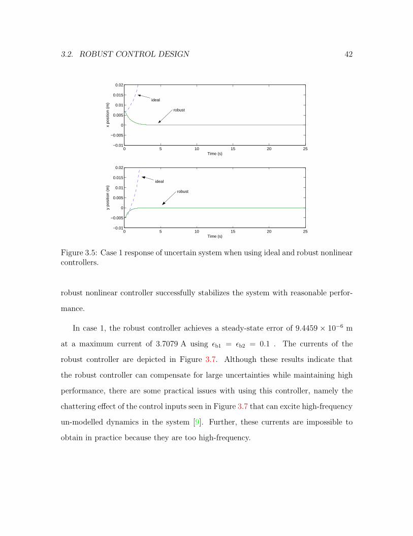
3.5 Case 1 response of uncertain system when using ideal and robust nonlinear controllers. 42
3.6 Case 1 response of uncertain system when using a linear controller and the robust nonlinear con
3.7 Currents of robust nonlinear controller in system subject to case 1. . 43
3.8 Case 1 response of uncertain system when using adaptive nonlinear controllers. 53
3.9 Case 2 response of uncertain system when using linear, robust and adaptive nonlinear controllers.
3.10 Control input of adaptive controller in case 2. . . . . . . . . . . . . . 55
3.11 Case 1 response of uncertain system when using the robust adaptive controller. 72
vii
LIST OF FIGURES LIST OF FIGURES
3.12 Case 2 response of uncertain system when using robust, adaptive and robust adaptive nonlinear
3.13 Currents from robust adaptive controller when in case 2. . . . . . . . 74
3.14 Case 3 response of uncertain system when using linear, robust, adaptive and robust adaptive
4.1 Top view of planar magnetic levitation device. . . . . . . . . . . . . . 77
4.2 Side view of planar magnetic levitation device. . . . . . . . . . . . . . 78
4.3 Overview of interfaces in magnetic levitation device. . . . . . . . . . . 79
4.4 Input/Output relationship between PWM and electromagnet. . . . . 82
4.5 Pulse-width modulator wiring. . . . . . . . . . . . . . . . . . . . . . . 83
4.6 Current controller structure. . . . . . . . . . . . . . . . . . . . . . . . 84
4.7 Current controller circuit. . . . . . . . . . . . . . . . . . . . . . . . . 85
4.8 Summer operational amplifier. . . . . . . . . . . . . . . . . . . . . . . 86
4.9 Proportional-integral operational amplifier. . . . . . . . . . . . . . . . 86
4.10 PI control tracking reference current. . . . . . . . . . . . . . . . . . . 87
4.11 Linear guides mounted in an X-Y fashion. . . . . . . . . . . . . . . . 89
4.12 Laser reflected off a curved surface. . . . . . . . . . . . . . . . . . . . 91
4.13 Linear guide and sensor setup. . . . . . . . . . . . . . . . . . . . . . . 93
4.14 Interface between position controller and magnetic levitation device. . 94
4.15 Model B inductance samples using method 1. . . . . . . . . . . . . . 105
4.16 Model B inductance samples using method 2. . . . . . . . . . . . . . 105
4.17 Model A inductance expressions using method 1 and 2. . . . . . . . . 108
4.18 Two-magnet system experimental setup. . . . . . . . . . . . . . . . . 110
4.19 Two-magnet system diagram. . . . . . . . . . . . . . . . . . . . . . . 111
4.20 Run 1: Disk position using the linear controller in the two-magnet system.114
4.21 Run 1: Currents of linear controller in the two-magnet system. . . . . 114
4.22 Run 2: Disk position using the linear controller in the two-magnet system.115
4.23 Run 3: Disk position using the ideal controller in the two-magnet system.116
viii
LIST OF FIGURES LIST OF FIGURES
4.24 Run 3: Currents of ideal controller in the two-magnet system. . . . . 116
4.25 Run 4: Disk position using the ideal controller in the two-magnet system.116
4.26 Run 5: Disk position using the equivalent ideal controller. . . . . . . 122
4.27 Run 5: Currents from the equivalent ideal controller. . . . . . . . . . 122
4.28 Run 6: Disk position using the equivalent ideal controller. . . . . . . 122
4.29 Run 6: Currents from the equivalent ideal controller. . . . . . . . . . 123
4.30 Run 7: Disk position using the 2 DOF ideal controller. . . . . . . . . 126
4.31 Run 7: Currents from the 2 DOF ideal controller. . . . . . . . . . . . 126
4.32 Run 8: Disk position using the 2 DOF ideal controller. . . . . . . . . 127
4.33 Run 8: Currents from the 2 DOF ideal controller. . . . . . . . . . . . 127
4.34 Response of disk from acceleration test. . . . . . . . . . . . . . . . . . 128
4.35 Currents from the acceleration test. . . . . . . . . . . . . . . . . . . . 128
A.1 Fringing between two magnets. . . . . . . . . . . . . . . . . . . . . . 132
A.2 Magnetic flux density plot for narrow magnets. . . . . . . . . . . . . . 134
A.3 Magnetic flux density plot for wide magnets. . . . . . . . . . . . . . . 135
A.4 Magnetic flux density plot for wider sized magnets. . . . . . . . . . . 136
ix

Chapter 1
Introduction
1.1 Motivation
The semiconductor industry is forced to refine the photolithography process to ac-
commodate the increasing need of denser integrated circuits. Photolithography is
a step in semiconductor production where patterns from a mask are drawn on a
photo-sensitive silicon wafer using an optical system. The linewidths of this pattern
are steadily decreasing and are created on silicon wafers of increasing diameter, e.g.
past generation requirements were linewidths of 0.13 µm and 300 mm diameter silicon
wafers [8]. High-precision positioning stages capable of actuating large movements are
used in this process to supply the necessary incremental movement on the wafer such
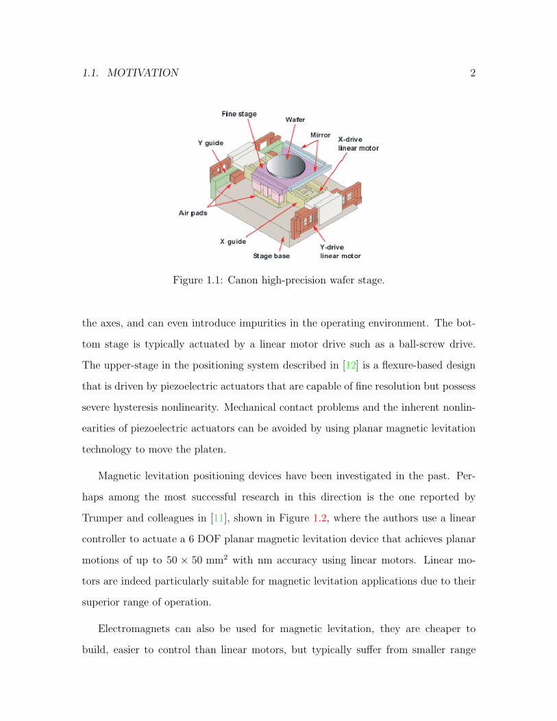
that the pattern is drawn on correctly. Figure 1.1 is a diagram of a stage developed
by Canon.
Typically, in industry, these positioning systems are comprised of a lower-stage
that actuates large high-speed movements and an upper-stage that delivers high-
precision movements in multiple degrees of freedom [12]. The mechanical contact
between the platen and the stage introduces friction, vibrations, coupling between
1
1.1. MOTIVATION 2
Figure 1.1: Canon high-precision wafer stage.
the axes, and can even introduce impurities in the operating environment. The bot-
tom stage is typically actuated by a linear motor drive such as a ball-screw drive.
The upper-stage in the positioning system described in [12] is a flexure-based design
that is driven by piezoelectric actuators that are capable of fine resolution but possess
severe hysteresis nonlinearity. Mechanical contact problems and the inherent nonlin-
earities of piezoelectric actuators can be avoided by using planar magnetic levitation
technology to move the platen.
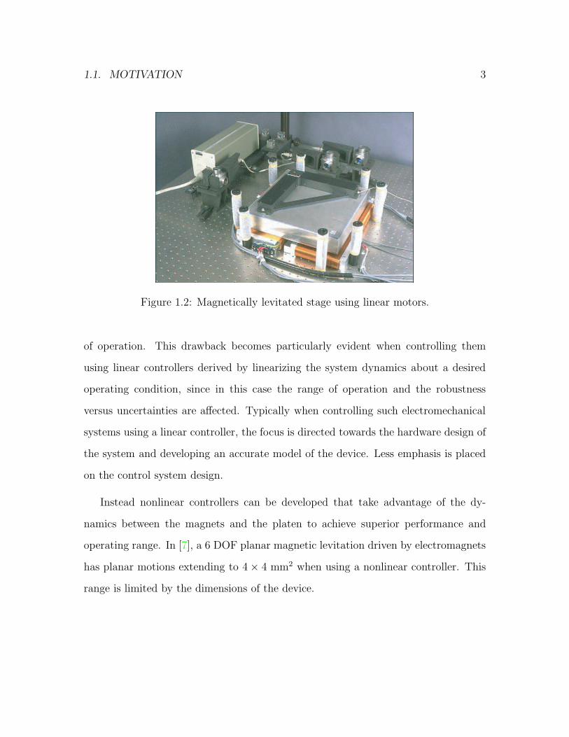
Magnetic levitation positioning devices have been investigated in the past. Per-
haps among the most successful research in this direction is the one reported by
Trumper and colleagues in [11], shown in Figure 1.2, where the authors use a linear
controller to actuate a 6 DOF planar magnetic levitation device that achieves planar
motions of up to 50 × 50 mm2 with nm accuracy using linear motors. Linear mo-
tors are indeed particularly suitable for magnetic levitation applications due to their
superior range of operation.
Electromagnets can also be used for magnetic levitation, they are cheaper to
build, easier to control than linear motors, but typically suffer from smaller range
1.1. MOTIVATION 3
Figure 1.2: Magnetically levitated stage using linear motors.
of operation. This drawback becomes particularly evident when controlling them
using linear controllers derived by linearizing the system dynamics about a desired
operating condition, since in this case the range of operation and the robustness
versus uncertainties are affected. Typically when controlling such electromechanical
systems using a linear controller, the focus is directed towards the hardware design of
the system and developing an accurate model of the device. Less emphasis is placed
on the control system design.
Instead nonlinear controllers can be developed that take advantage of the dy-
namics between the magnets and the platen to achieve superior performance and
operating range. In [7], a 6 DOF planar magnetic levitation driven by electromagnets
has planar motions extending to 4 × 4 mm2 when using a nonlinear controller. This
range is limited by the dimensions of the device.

1.2. PROBLEM FORMULATION 4
1.2 Problem Formulation
In this thesis, we focus on a planar magnetic levitation device which employs electro-
magnets to achieve 2 DOF, while keeping a relatively large operating range. To avoid
the limitations mentioned above, we develop a rigorous nonlinear control framework
to solve the stabilization problem over a guaranteed range, and apply various control
techniques to make the closed-loop system robust versus a class of uncertainties. The
electromechanical system considered includes the triangular arrangement shown in
Figure 1.3 which differs from most magnetic levitation positioning devices. Using the
minimum number of electromagnets required to actuate two degrees of freedom in a
triangular arrangement was explicitly chosen to create a challenging and interesting
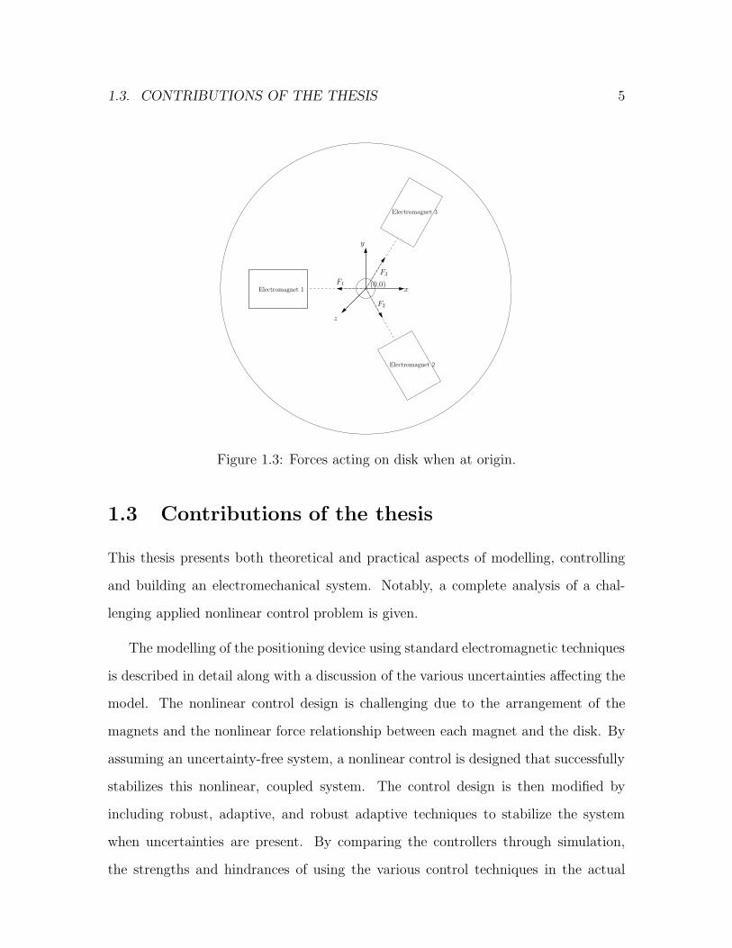
nonlinear control design problem. Figure 1.3 demonstrates a plan view of the system
and the forces exerted on the disk by each magnet. Each of the rectangles represents
an electromagnet with a ferromagnetic core with N coil windings. The circle in the
middle of the plane is a disk, also of ferromagnetic material, whose position we want
to control.
The full realization of the system would include a fourth magnet suspended above
the three magnets shown. The additional magnet producing a force in the z direction
is independent of the magnets in the xy plane (at least theoretically). That is, the
system is comprised of two decoupled subsystems - the base magnets formed in a
triangle and the suspended magnet above this plane. The focus of this research is on
the xy subsystem.
1.3. CONTRIBUTIONS OF THE THESIS 5
F1
F3
F2
Electromagnet 1
Electromagnet 2
Electromagnet 3
(0,0)
z
y
x
Figure 1.3: Forces acting on disk when at origin.
1.3 Contributions of the thesis
This thesis presents both theoretical and practical aspects of modelling, controlling
and building an electromechanical system. Notably, a complete analysis of a chal-
lenging applied nonlinear control problem is given.
The modelling of the positioning device using standard electromagnetic techniques
is described in detail along with a discussion of the various uncertainties affecting the
model. The nonlinear control design is challenging due to the arrangement of the
magnets and the nonlinear force relationship between each magnet and the disk. By
assuming an uncertainty-free system, a nonlinear control is designed that successfully
stabilizes this nonlinear, coupled system. The control design is then modified by
including robust, adaptive, and robust adaptive techniques to stabilize the system
when uncertainties are present. By comparing the controllers through simulation,
the strengths and hindrances of using the various control techniques in the actual

1.4. ORGANIZATION OF THE THESIS 6
positioning device are outlined.
On the practical side, a prototype of the magnetic levitation device is built and
can potentially be used to test nonlinear controllers and their ability to compensate
for uncertainties. The hardware design of the testbed is described and, although, due
to hardware limitations, the controllers could not be tested, significant modelling and
control results are given and discussed using simpler testbeds.
1.4 Organization of the thesis
The document is divided into three main parts: modelling, nonlinear control design,
and implementation. Chapter 2 develops a mathematical model describing the three-
magnet positioning system. The basic electromagnetic analysis needed to derive the
dynamics of the disk from a single magnet is first derived in Section 2.1. In Section
2.2 this one-dimensional result is expanded in the xy plane to find the equations of the
forces acting on the disk from all three magnets, which we then use to find the state-
space representation of the disk dynamics shown in Section 2.3. The chapter is closed
in Section 2.4 with a discussion of the uncertainties of the model due to some as-
sumptions made. Background information is available in Appendix A which includes
the analysis of the different configurations considered for the triangular arrangement.
The nonlinear control design of the system is presented in the third chapter. In
Section 3.1 we assume the model developed in Chapter 2 is not affected by uncertain-
ties and derive a feedback transformation yielding linear dynamics. In the transformed
domain, an LQR controller is designed to complete the feedback loop and stabilize
the system. In the next three sections, uncertainties in the model are considered and
various control schemes that handle these uncertainties are developed. Specifically,

1.4. ORGANIZATION OF THE THESIS 7
in Section 3.2 Lyapunov redesign is performed to robustify the ideal controller de-
veloped in Section 3.1. Alternatively, the uncertainties can be compensated using a
classic adaptive controller, developed in Section 3.3. Lastly, Section 3.4 describes a
robust adaptive control that combines the uncertainty handling notions of robust and
adaptive techniques. Simulations comparing the system response of the ideal, robust,
adaptive and robust adaptive controllers are given in each section.
The fourth chapter features the actual hardware implementation of the planar
magnetic device. In Section 4.1, the electromechanical positioning device is described
by explaining the individual components used to build the system and their mu-
tual interactions. Although, due to hardware difficulties, the testbed is not fully
operational, two smaller experiments were designed to reveal the problem in the
three-magnet system and experimentally verify some modelling and control aspects
discussed in the second and third chapters. The results achieved with these testbeds
are fairly encouraging and substantial.
The document is finalized with a summary of the main objectives achieved along
with some recommendations on the hardware design and possible future prospects of
the research.
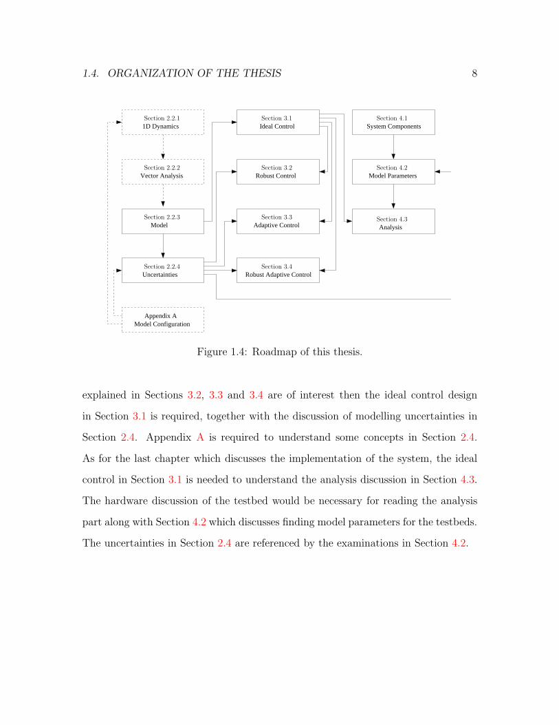
For readability purposes, a roadmap of this thesis explaining the relationships
between sections in this document is included in Figure 1.4. Sections 2.1 and 2.2
can be considered optional although they give insight into the modelling and some
parts are referenced when analyzing the testbed in Section 4.2. Similarly, Appendix
A gives reasons why this particular magnet configuration is being used and provides
some background on electromagnetic concepts. For the control design, the reader may
skip the uncertainty compensating controllers and focus on the ideal control design
detailed in Section 3.1. In that case, one just needs to read Section 2.3, where the
state-space model is given. If the robust, adaptive, or the robust adaptive controls
1.4. ORGANIZATION OF THE THESIS 8
Robust Control
Ideal Control
AnalysisAdaptive Control
Robust Adaptive Control
System Components
Model Parameters
1D Dynamics
Model ConfigurationAppendix A
Uncertainties
Model
Vector AnalysisSection 4.2
Section 4.1
Section 3.2
Section 3.1
Section 3.3
Section 3.4
Section 2.2.1
Section 2.2.4
Section 2.2.3
Section 2.2.2
Section 4.3
Figure 1.4: Roadmap of this thesis.
explained in Sections 3.2, 3.3 and 3.4 are of interest then the ideal control design
in Section 3.1 is required, together with the discussion of modelling uncertainties in
Section 2.4. Appendix A is required to understand some concepts in Section 2.4.
As for the last chapter which discusses the implementation of the system, the ideal
control in Section 3.1 is needed to understand the analysis discussion in Section 4.3.
The hardware discussion of the testbed would be necessary for reading the analysis
part along with Section 4.2 which discusses finding model parameters for the testbeds.
The uncertainties in Section 2.4 are referenced by the examinations in Section 4.2.

Chapter 2
Modelling of the Planar Magnetic
Levitation Device
In this chapter, a set of differential equations describing the motion of the disk in our
planar positioning device is developed.
The equations describing the motion of the disk are
x =Fx(x, y, I1, I2, I3)
m
y =Fy(x, y, I1, I2, I3)
m,
(2.0.1)
where m is the mass of the disk. The forces Fx and Fy are the forces generated by
the three electromagnets with currents I1, I2, I3 in the x and y direction, respectively.
In this section we develop a mathematical model of the system depicted in Figure 1.3
using superposition of the forces and neglecting the fringing effect of the magnetic
flux lines. The following assumptions are made throughout the modelling process and
in other parts of the thesis:
Assumption 2.0.1. Fringing of the magnetic flux lines is negligible.
9

CHAPTER 2. MODELLING OF THE PLANAR MAGNETIC LEVITATION DEVICE10
Assumption 2.0.2. Flux leakage through the coils of the electromagnets is negligible.
Assumption 2.0.3. The relationship between the magnetic flux density, ~B, and the
magnetic field intensity, ~H, is linear.
Assumption 2.0.4. Currents vary slowly so a constant-current method can be used.
Assumption 2.0.5. Magnetic flux is contained throughout the Amperian path.
Assumption 2.0.6. The disk remains within the region where superposition holds.
Assumption 2.0.7. The attractive forces acting on the disk point towards the center
of each magnet face.
Assumption 2.0.8. The length of each core is sufficiently larger than the width and
height of the core.
Assumption 2.0.9. The uncertainty term θ2 |x3| in the expression (2.4.2) in Section
2.4 is negligible for the adaptive and robust adaptive control designs.
These assumptions are described later in Section 2.4 in terms of the modelling un-
certainties they may introduce. The dynamics of the disk can be modelled in four
steps.
1. Derive the dynamics of the forces acting on the disk from a single electromagnet.
2. Using the result in step 1, perform vector analysis to construct the force dy-
namics of the disk from all three electromagnets.
3. Use the result from step 2 in motion equations (2.0.1).
4. Find state-space representation.

2.1. FORCE DYNAMICS OF DISK FROM SINGLE ELECTROMAGNET 11
2.1 Force Dynamics of Disk from Single Electro-
magnet
This analysis is standard and the result can be found in, e.g. in [13]. The forces are
calculated by taking the gradient of the system’s magnetic energy. Magnetic energy
can be calculated from the magnetic flux. Thus, the first step is to find the magnetic
flux through the core of the electromagnets. Magnetic flux is found using Ampere’s
Law [1]∮
C
~H · d~l = µoIenc. (2.1.1)
Ampere’s law states that the line integral of H around any closed path C equals
the product of the current Ienc enclosed by the path and the permeability of free space
µo [1]. It can be restated as follows
∮
C
~H · d~l = NI, (2.1.2)
where N is the number of coil windings and I is the current going through the coils.
Magnetic field lines, ~H , and magnetic flux density lines, ~B, have the same direction
in a ferromagnetic material when the core is not saturated [3]. Assuming the core
never enters saturation, the relationship between ~B and ~H is linear,
~H =1
µ~B. (2.1.3)
where µ is the core permeability. The magnetic flux can be calculated in terms of the
magnetic flux density and cross sectional area of the core
Φ =
∫
S
~B · d~s. (2.1.4)
2.1. FORCE DYNAMICS OF DISK FROM SINGLE ELECTROMAGNET 12
It is common to assume that the magnitude of the magnetic flux is constant, therefore
the expression becomes
Φ = BA, (2.1.5)
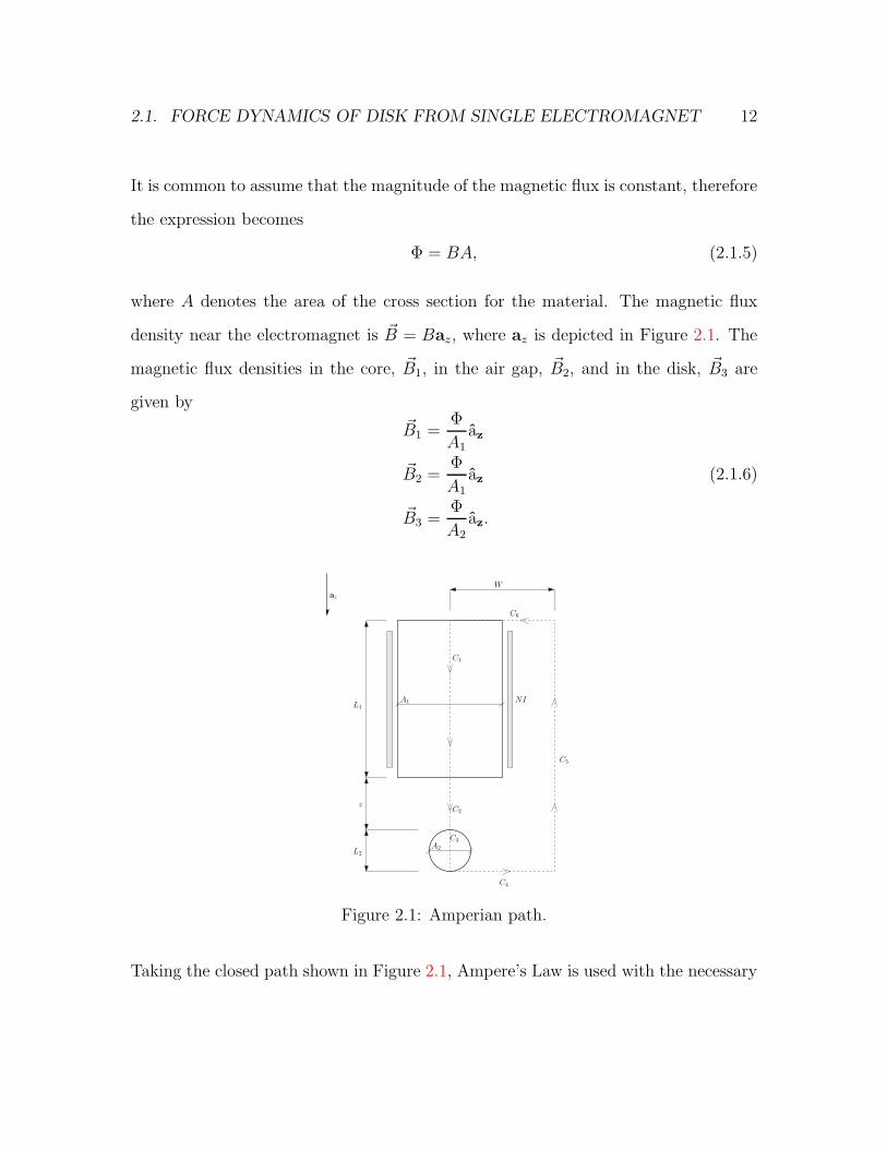
where A denotes the area of the cross section for the material. The magnetic flux
density near the electromagnet is ~B = Baz, where az is depicted in Figure 2.1. The
magnetic flux densities in the core, ~B1, in the air gap, ~B2, and in the disk, ~B3 are
given by
~B1 =Φ
A1
az
~B2 =Φ
A1
az
~B3 =Φ
A2
az.
(2.1.6)
C1
C4
C5
C6
W
L2
z
L1
C3
C2
NIA1
A2
az
Figure 2.1: Amperian path.
Taking the closed path shown in Figure 2.1, Ampere’s Law is used with the necessary

2.1. FORCE DYNAMICS OF DISK FROM SINGLE ELECTROMAGNET 13
substitutions from equations (2.1.3) and (2.1.6) to get magnetic flux. Thus
∮
C
~H · d~l =
∮
C
1
µ~B · d~l
=
∮
C1
1
µ1
~B1 · d~l +∮
C2
1
µo
~B2 · d~l +∮
C3
1
µ2
~B3 · d~l + 0 +
∮
C5
1
µo
~0 · d~l + 0
=L1
µ1
Φ
A1+
z
µo
Φ
A1+L2
µ2
Φ
A2
=
(
L1
µ1A1
+L2
µ2A2
+z
µoA1
)
Φ
= NI.
The line integrals corresponding to C4 and C6 are zero because ~B is perpendicular
to the lines C4 and C6. The line integral corresponding to C5 can be assumed zero by
assuming that the lengths of C4 and C6 stretch to infinity. Thus, the magnetic flux
reads as
Φ =NI
L1
µ1A1+ L2
µ2A2+ z
µoA1
. (2.1.7)
Remark 2.1.1. The last fraction in the denominator of (2.1.7), zµoA1
, is the reluctance
of the air gap between the core and the disk. Since fringing is neglected, it is assumed
that the cross-sectional area of the magnetic flux passing through the air gap is equal
to the cross-sectional area of the core. If fringing were not neglected, the cross-
sectional area of the air gap would be greater than that of the core, A1, and it would
vary in size depending on the length of the air gap, z. Thus the reluctance of the
air gap would instead read as zµoA3(z)
where A3(z) > A1. Fringing is illustrated in
Appendix A.1.
Magnetic energy is defined as
Wm =1
2
∫
V
~B · ~Hdv (2.1.8)
2.1. FORCE DYNAMICS OF DISK FROM SINGLE ELECTROMAGNET 14
where V is the volume of the object subject to ~B and ~H .
Using the equations (2.1.3) and (2.1.6), the magnetic flux expression (2.1.7) and
(2.1.8), the magnetic energy of the system can be expressed as
Wm =1
2
∫
V
~B · ~Hdv
=1
2
∫
V
1
µB2dv
=1
2
[∫
V1
1
µ1
(
Φ
A1
)2
dv +
∫
V2
1
µo
(
Φ
A1
)2
dv +
∫
V3
1
µ2
(
Φ
A2
)2
dv
]
=1
2
[
L1A1
µ1A21
Φ2 +zA1
µoA21
Φ2 +L2A2
µ2A22
Φ2
]
=Φ2
2
[
L1
µ1A1
+z
µoA1
+L2
µ2A2
]
=(NI)2
2
1L1
µ1A1+ L2
µ2A2+ z
µ0A1
,
where B denotes the magnitude of ~B, h is the height of the disk and A2 = L2h is the
cross-sectional area of the disk.
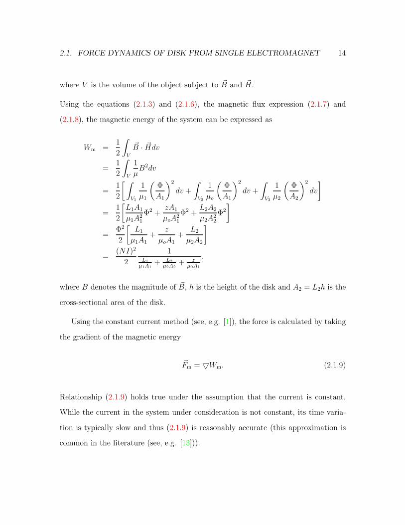
Using the constant current method (see, e.g. [1]), the force is calculated by taking
the gradient of the magnetic energy
~Fm = 5Wm. (2.1.9)
Relationship (2.1.9) holds true under the assumption that the current is constant.
While the current in the system under consideration is not constant, its time varia-
tion is typically slow and thus (2.1.9) is reasonably accurate (this approximation is
common in the literature (see, e.g. [13])).

2.2. VECTOR ANALYSIS AND SYSTEM DYNAMICS 15
Using equation (2.1.9) the force acting on the disk by one electromagnet is
~Fm = 5Wm
=∂Wm
∂zaz
= − (NI)2
2µ0A1
1(
L1
µ1A1+ L2
µ2A2+ z
µ0A1
)2az.
(2.1.10)
Similarly to the standard result, the one-dimensional force expression is proportional
to the current squared and to the reciprocal of the distance squared.
2.2 Vector Analysis and System Dynamics
Using superposition and the results from the previous section, we next derive the
forces acting on the disk from all three magnets. The force expression for a single
magnet is used in vector analysis to get the force equations of the entire system. The
force model of the system is as follows
~Fx = (F1 cos θ1 + F2 cos θ2 + F3 cos θ3) ax
~Fy = (F1 sin θ1 + F2 sin θ2 + F3 sin θ3) ay.
(2.2.1)
Figure 2.2 shows the angles θ1, θ2, θ3 and the forces acting on the disk when it is at a
location (x, y) inside the triangle 4P1P2P3, which is assumed to be equilateral. The
attractive force from electromagnet i, where i = 1, 2, 3, has the expression
~Fi = −(NIi)2
2µ0A1
1(
L1
µ1A1+ L2
µ2A2+ zi
µ0A1
)2azi. (2.2.2)
2.2. VECTOR ANALYSIS AND SYSTEM DYNAMICS 16
1
3
P1
P2
2
P3
w
l
z3
(0,0)
z1
y
x
az3
az2
az1
(x,y)
θ1
z2
θ3
θ2
d
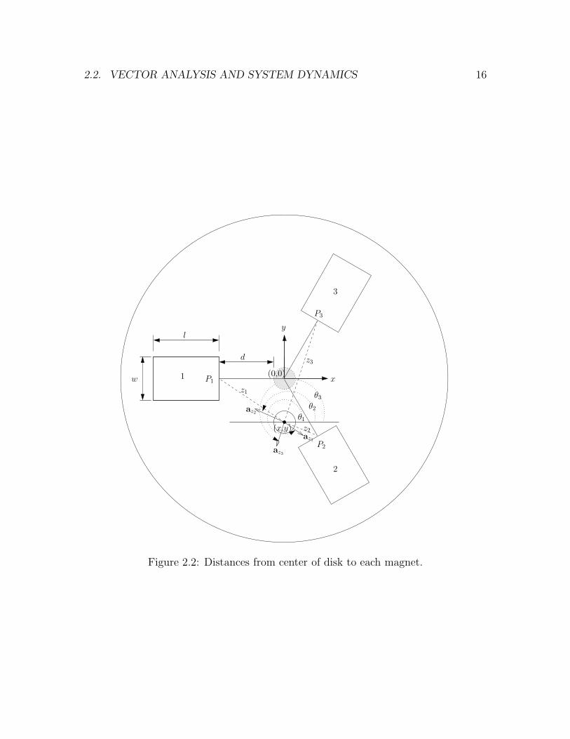
Figure 2.2: Distances from center of disk to each magnet.
2.2. VECTOR ANALYSIS AND SYSTEM DYNAMICS 17
The value zi, depicted in Figure 2.2, is the distance between the edge of the disk and
the middle point, denoted Pi, of the face of electromagnet i. The distance between
the disk’s edge when at the origin and the face of each magnet is d. The direction of
the force exerted by each ith electromagnet is the unit vector azi, depicted in Figure
2.2. This unit vector changes with the disk’s position and is defined as
azi=
−~Fi∣
∣
∣
~Fi
∣
∣
∣
.
Next, zi can be expressed as
z1 = ‖(x, y) − P1‖
= ‖(x, y) − (−d, 0)‖
=√
(x+ d)2 + y2
z2 = ‖(x, y) − P2‖
=
∥
∥
∥
∥
∥
(x, y) −(
d
2,−
√3
2d
)
∥
∥
∥
∥
∥
=
√
(
x− d
2
)2
+
(
y +
√3
2d
)2
z3 = ‖(x, y) − P3‖
=
√
(
x− d
2
)2
+
(
y −√
3
2d
)2
.
(2.2.3)
The next step is to express sin θi and cos θi in terms of x and y. From Figure 2.2, it
can be shown that
sin θ1 =−yz1
cos θ1 =x+ d
z1
2.2. VECTOR ANALYSIS AND SYSTEM DYNAMICS 18
sin θ2 =y +
√3
2d
z2
cos θ2 =x− d
2
z2
sin θ3 =y −
√3
2d
z3
cos θ3 =x− d
2
z3.
By substituting the variable distances zi and putting the trigonometric functions in
terms of x and y, the Fx equation in (2.2.1) becomes
Fx = F1 cos θ1 + F2 cos θ2 + F3 cos θ3
= − 1
2µoA1
[
(N1I1)2
(
L1
µ1A1+ L2
µ2A2+ z1
µ0A1
)2
x+ d
z1+
(N2I2)2
(
L1
µ1A1+ L2
µ2A2+ z2
µ0A1
)2
x− d2
z2+
(N3I3)2
(
L1
µ1A1+ L2
µ2A2+ z3
µ0A1
)2
x− d2
z3
]
= − 1
2µoA1
[
(N1I1)2
(
L1
µ1A1+ L2
µ2A2+
√(x+d)2+y2
µ0A1
)2
x+ d√
(x+ d)2 + y2+
(N2I2)2
L1
µ1A1+ L2
µ2A2+
s
(
x− d2
)2
+
(
y+√
3
2d
)2
µ0A1
2
x− d2
√
(
x− d2
)2
+(
y +√
32d)2
+
(N3I3)2
L1
µ1A1+ L2
µ2A2+
s
(
x− d2
)2
+
(
y−√
3
2d
)2
µ0A1
2
x− d2
√
(
x− d2
)2
+(
y −√
32d)2
]
,
where N1, N2, N3 are the number of windings of electromagnets 1,2 and 3 shown in
2.3. STATE-SPACE REPRESENTATION OF MOTION EQUATIONS 19
Figure 1.3. Similarly for the force exerted on the disk in the y direction
Fy = − 1
2µoA1
[
(N1I1)2
(
L1
µ1A1+ L2
µ2A2+
√(x+d)2+y2
µ0A1
)2
−y√
(x+ d)2 + y2+
(N2I2)2
L1
µ1A1+ L2
µ2A2+
s
(
x− d2
)2
+
(
y+√
3
2d
)2
µ0A1
2
y +√
32d
√
(
x− d2
)2
+(
y +√
32d)2
+
(N3I3)2
L1
µ1A1+ L2
µ2A2+
s
(
x− d2
)2
+
(
y−√
3
2d
)2
µ0A1
2
y −√
32d
√
(
x− d2
)2
+(
y −√
32d)2
]
.
All that remains is substituting these force expressions into the motion equations
(2.0.1) to find the state space representation.
2.3 State-Space Representation of Motion Equa-
tions
Define the state of the system as
x =
x1
x2
x3
x4
:=
x
x
y
y
. (2.3.1)
Using this definition and substituting the force expressions into motion equations
2.3. STATE-SPACE REPRESENTATION OF MOTION EQUATIONS 20
(2.0.1) gives the dynamics of the entire system
x1 = x2
x2 = − 1
2mµoA1
[
ϕ1(x1, x3)(x1 + d)I21 + ϕ2(x1, x3)
(
x1 −d
2
)
I22
+ ϕ3(x1, x3)
(
x1 −d
2
)
I23
]
x3 = x4
x4 = − 1
2mµoA1
[
ϕ1(x1, x3)(−x3)I21 + ϕ2(x1, x3)
(
x3 +
√3
2d
)
I22
+ ϕ3(x1, x3)
(
x3 −√
3
2d
)
I23
]
(2.3.2)
where
ϕ1(x1, x3) =N2
1(
L1
µ1A1+ L2
µ2A2+
√(x1+d)2+x2
3
µ0A1
)2√
(x1 + d)2 + x23
ϕ2(x1, x3) =N2
2
L1
µ1A1+ L2
µ2A2+
s
(
x1− d2
)2
+
(
x3+√
3
2d
)2
µ0A1
2√
(
x1 − d2
)2
+(
x3 +√
32d)2
ϕ3(x1, x3) =N2
3
L1
µ1A1+ L2
µ2A2+
s
(
x1− d2
)2
+
(
x3−√
3
2d
)2
µ0A1
2√
(
x1 − d2
)2
+(
x3 −√
32d)2
.
The state-space representation of the motion equations for the disk is complete. Table
2.1 lists values of various physical constants in the system used for simulations and
other analysis.

2.4. UNCERTAINTIES 21
Parameter Valueµ0 4π × 10−7
µr 700µ1 2.8π × 10−4
µ2 2.8π × 10−4
L1 0.1000 mL2 0.0167 md 0.0500 mm 0.5000 kgh 0.0083 mN 100A1 0.01 m2
A2 1.39 × 10⁻⁴ m2
Table 2.1: Values of physical parameters.
2.4 Uncertainties
The mathematical representation of the planar magnetic levitation device is subject
to uncertainties. Uncertainties are present in this model due to the assumptions made
during the modelling: friction that was not accounted for, force direction estimates
and neglected fringing effects. They are represented in the system as follows
x1 = x2
x2 =Fx(x1, x3, I1, I2, I3)
m+δ2(x)
m
x3 = x4
x4 =Fy(x1, x3, I1, I2, I3)
m+δ4(x)
m,
(2.4.1)
where δ2(x) and δ4(x) represent unknown forces that can be generated from various
electromagnetic modelling assumptions not holding, as well as friction. Such unknown

2.4. UNCERTAINTIES 22
forces are assumed to have structurally known upper bound as follows
δ2(x) = ∆2(x1, x3) − θ3x2, |∆2(x1, x3)| ≤ θ1 |x1| + θ2 |x3|
δ4(x) = ∆4(x1, x3) − θ6x4, |∆4(x1, x3)| ≤ θ4 |x1| + θ5 |x3|(2.4.2)
where θi ∈ <p, for i = 1, .., 6, are unknown parameters and the terms −θ3x2, −θ6x4
represent viscous friction. Notice that θi above is not to be confused with the force
angles shown in Figure 2.2. The terms ∆2(x1, x3) and ∆4(x1, x3) are upper bounds
to unknown forces that can be generated from one or a combination of Assumptions
2.0.1, 2.0.2, 2.0.3, 2.0.4, 2.0.5, 2.0.6, 2.0.7, and 2.0.8 not holding.
Our model was developed using various assumptions. Assumptions 2.0.1, 2.0.3,
2.0.4, and 2.0.5 were indicated when developing the dynamics of the one-dimensional
result. Although it is necessary to assume that fringing and flux leakage are negligible
to develop this model, assumptions 2.0.1 and 2.0.2, there is definitely fringing and
at least some flux leakage in the actual system. Thus these are regarded as possible
source of uncertainty. Fringing is described in Appendix A.1 and flux leakage is
described later in this section.
The B − H relationship is linear when the material used for the electromagnet
cores is homogeneous, linear and isotropic [1]. Although these properties hold for
soft ferromagnetic materials such as soft iron, Assumption 2.0.3 is still regarded as a
possible source of uncertainty.
Assumption 2.0.4 is realistic as well. The only time the currents vary considerably
is during the transient of the - when the currents begin changing to stabilize the disk
at a position. The current variations during this time could cause problems with the
accuracy of the model.
Magnetic flux is typically assumed constant in literature when, for instance, the

2.4. UNCERTAINTIES 23
flux lines travel within a high-permeability core through a small air-gap [1]. The cores
used in this case are ferromagnetic and have a large permeability. However, the air
gaps between the cores and the disk are not small and the resulting fringing from this
implies that the magnetic flux at the disk may be significantly less then the Φ going
through the electromagnet. Flux lines follow the path inside the material with least
reluctance and air has a large reluctance. Therefore intuitively speaking, the larger
the air gap the less flux lines will reach the disk. Further, regardless of air gap size
and core permeability, flux leakage between the coils of the magnets decreases the
amount of magnetic flux going through the air gap, as depicted in Figure 2.3. Even
though the coils are wound tightly and wound to the ends of the core, the magnetic
field between the coils may not be entirely cancelled. Fringing and flux leakage make
Assumption 2.0.5 a source of uncertainty.
I
flux leakage
Figure 2.3: Flux leakage of an electromagnet.
The model was built using Assumption 2.0.6, as discussed in Appendix A.2. It is
known that superposition holds when the disk is at the origin. If the disk is moved
at a position where superposition does not hold then the model derived does not
represent the system. Measures are taken in the control design to compensate for the
possibility of superposition not holding. If superposition, or any other uncertainty

2.4. UNCERTAINTIES 24
for that matter, was not taken into account in the control design then the controller
would output incorrect currents because its results would be based on an incorrect
model. It would therefore be difficult for a controller that assumes the disk never
goes outside the region where superposition holds to stabilize the disk.
The assumption that the forces are directed towards the center of each magnet,
Assumption 2.0.7, is depicted in Figure 1.3. However, as the disk approaches the
face of a magnet, the force exerted on the disk may point towards the part of the
magnet closest to the disk. Realistically, the disk must be confined in an area that is
sufficiently far from all the magnets for this assumption to hold. The mathematical
model we derived does not express the system correctly if the disk is outside of this
region and, thus, the controller must be able to compensate for the presence of this
uncertainty.
Furthermore, the areas where Assumptions 2.0.6 and 2.0.7 hold change in size as
the controller adjusts the currents to stabilize the disk.
Assumption 2.0.8 deals with length of the cores being greater than the both the
height and width of the cores, that is L1 >> A1. The reason is given when discussing
magnets in Section 4.1 of the implementation chapter. Assumption 2.0.9 concerns
the uncertainty term θ2 |x3| in equation (2.4.2). In the adaptive and robust adaptive
control designs it is necessary to impose the requirement that θ2 = 0. This assumption
is discussed further and tested via simulation in Section 3.3, the adaptive control
design, and in Section 3.4, the robust adaptive control design.
The two degrees of freedom of the planar magnetic levitation device are coupled
because of the three-magnet arrangement and hence ∆2 and ∆4 depend on x and y
position of the disk, i.e., ∆2 = ∆2(x1, x3), ∆4 = ∆4(x1, x3). To further illustrate this
point, for a positive small number ε, consider two scenarios: in first case the disk is
initially at (0, 0) and the desired final position is (0, ε); and in the second scenario the

2.4. UNCERTAINTIES 25
disk starts at (0, ε) and the desired final position is (ε, ε). In the second case, the disk
starts at a position where uncertainties are more significant: the disk may be out of
the region where superposition holds, or perhaps at this position the attractive forces
generated by electromagnet 1 and 3 are not directed towards their centers. In terms
of control, it will be more difficult to move the disk in the x direction from (0, ε) to
(ε, ε) than from (0, 0) to (ε, 0). Uncertainties ∆2 and ∆4 are therefore a function of
(x, y).
In the implementation, the disk is not being levitated by a magnet in the z di-
rection but instead is anchored onto a movable platform that rides on ball bearings.
Although ball bearings enable smooth movement, friction was not included in the
modelling and therefore the last term in the uncertainties δ2 and δ4 includes a viscous
friction expression with unknown coefficients θ3, θ6. However, the friction from the
mechanical contact between the ball bearings and the platform is more accurately
represented by Coulomb friction. This was not considered in the modelling or the
control design and the effect of this is discussed in Section 4.3.3.
Lastly, the platen being moved by the electromagnets was chosen to be a disk
instead of a square so the force acting on the disk from each magnet is equivalent.
Consider if the platen in Figure 1.3 was square shaped. The force exerted on the
platen from electromagnet 1 would differ from those by electromagnet 2 and 3 because
magnet 1 is dealing with a different cross-sectional area than magnets 2 and 3. The
square platform would complicate the model because different force dynamics would
have to be developed for each separate magnet. The disk platen simplifies the model
and avoids possible added uncertainty.

Chapter 3
Nonlinear Control Design
Focussing on the coupled nonlinear xy subsystem at the base, we initiate a research
that aims to develop a rigorous nonlinear control framework to solve the set point
regulation problem for such systems. The controller first converts the magnet-disk
dynamics into a linear system in Brunovsky normal form and then using either robust,
adaptive or robust adaptive techniques to compensate for model uncertainties, the
three-magnet planar magnetic levitation system is stabilized.
Position
Controller
Nonlinear
Transformation
x
xrefPlant
−+
I1, I2, I3u1, u2
Figure 3.1: Overview of control system.
The two major issues dealt with are
1. Constructing a control law that converts the nonlinear model into a simpler
system.
26

3.1. IDEAL CONTROL DESIGN 27
2. Designing a controller that compensates for the uncertainties present in the
system while achieving high performance with minimal control effort.
Figure 3.1 shows the basic structure of the position feedback loop for the planar levi-
ation device. The framework for solving issue 1 is demonstrated in Section 3.1. The
first part develops expressions for three currents needed to transform the nonlinear
system into a linear system. The feedback loop is completed by designing an LQR
controller. The stable response of this ideal control system is shown when used in the
nominal system. In Section 3.2, the ideal controller is robustified to handle uncertain-
ties in the system. Simulations comparing the robust controller with the ideal and
linear controllers are shown when used in the system with uncertainties present. In
Section 3.3, an adaptive controller is designed and simulation results are later shown
comparing it with the linear and robust controllers. In the last part of the chap-
ter, Section 3.4, a robust adaptive controller is developed. Simulations comparing
this controller with the linear, robust and adaptive controller are then shown. The
chapter concludes with a discussion on the most suitable controller to be used in the
actual system.
3.1 Ideal Control Design
In this section, the design of a nonlinear controller that provides asymptotic stabi-
lization to the origin is described. The ideal controller does not take uncertainties
into account, thus we are considering the nominal model when δ2 = 0 and δ4 = 0 in
(2.4.2).

3.1. IDEAL CONTROL DESIGN 28
Proposition 3.1.1. There exists a feedback transformation for system (2.3.2),
I21
I22
I23
= T (x,u),
where u = [u1, u2]> and T : <4 × <2 → <3 is well-defined over the set
C =
x ∈ <4,u ∈ <2 : |x1| ≤d
6, |x3| ≤
d
6
, (3.1.1)
such that the dynamics in the transformed input domain read as
x1 = x2
x2 = u1
x3 = x4
x4 = u2,
(3.1.2)
where u1 and u2 are the new control inputs after feedback transformation.
Remark 3.1.1. Note that the feedback transformation in Proposition 3.1.1 is not a
standard feedback linearizing one in that while the original system (2.3.2) has three
positive inputs, the transformed system (3.1.2) is linear with two inputs.
In other words we seek to find a feedback transformation converting (at least on
a suitable compact set) the dynamics (2.3.2) into a linear system where a well-known
linear control technique can be applied to stabilize the entire system. Because the
control enters the system squared, the main difficulty in the design is finding positive
functions for I2i whose combination results in (3.1.2).
Proof. The solution presented here is a generalization of an idea presented in [10],
3.1. IDEAL CONTROL DESIGN 29
Section 12.3. Attaining x2 = u1 and x4 = u2 can be more easily achieved by rewriting
x1 = x2
x2 − x4 = u1 − u2 (3.1.3)
x3 = x4
x2 = u1. (3.1.4)
The control design can be broken down into three steps
1. Finding smooth positive functions for I21 , I2
2 and I23 that satisfy equation (3.1.3).
2. Substitute I21 , I2
2 and I23 found in step 1 into (3.1.4) and use the available degrees
of freedom to satisfy equation (3.1.4).
3. Using LQR, design a gain matrix that renders the closed-loop system stable.
In the first part, smooth functions must be found to make x2 − x4 become u1 − u2.
The three currents must cooperate together to supply a function that satisfies (3.1.3).
Similarly to what is done in [10], Section 12.3, we use the following expressions for
the currents
I21 =
−2mµ0A1
ϕ1(x1, x3)(x1 + x3 + d)η1(x1, x3, u1, u2)
I22 =
−2mµ0A1
ϕ2(x1, x3)(
x1 − x3 −√
3+12d)η2(x1, x3, u1, u2)
I23 =
−2mµ0A1
ϕ3(x1, x3)(
x1 − x3 +√
3−12d)η3(x1, x3, u1, u2),
(3.1.5)
where η1, η2 and η3 are degrees of freedom to be defined later. Substituting the

3.1. IDEAL CONTROL DESIGN 30
currents (3.1.5) into x2 − x4 gives
x2 − x4 = − 1
2mµ0A1
[
ϕ1(x1, x3)(x1 + x3 + d)I21
ϕ2(x1, x3) +
(
x1 − x3 −√
3 + 1
2d
)
I22
+ϕ3(x1, x3)
(
x1 − x3 +
√3 − 1
2d
)
I23
]
= − 1
2mµ0A1
[
ϕ1(x1, x3)(x1 + x3 + d)−2mµ0A1
ϕ1(x1, x3)(x1 + x3 + d)η1(·)
+ϕ2(x1, x3)
(
x1 − x3 −√
3 + 1
2d
)
−2mµ0A1
ϕ2(x1, x3)(
x1 − x3 −√
3+12d)η2(·)
+ϕ3(x1, x3)
(
x1 − x3 +
√3 − 1
2d
)
−2mµ0A1
ϕ3(x1, x3)(
x1 − x3 +√
3−12d)η3(·)
]
= η1(x1, x3, u1, u2) + η2(x1, x3, u1, u2) + η3(x1, x3, u1, u2), (3.1.6)
The signs of the functions η1, η2 and η3 must be such that I21 , I2
2 and I23 are all
positive. The function ϕi appearing in Ii is positive, for i = 1, .., 3, while the constant
−2mµ0A1 is negative. The denominators x1 + x3 + d and x1 − x3 +√
3−12d in (3.1.5)
are positive over the set C defined in (3.1.1), while the expression x1 − x3 −√
3+12d
in the denominator of I2 is always negative on C. Thus, in order to guarantee that
I21 , I
22 , I
23 are always positive, the signs of η1, η2 and η3 must be as follows
η1 ≤ 0, η2 ≥ 0 and η3 ≤ 0. (3.1.7)
The actual functions are now to be defined. These function must be smooth, obey
the sign constraints given in (3.1.7) and, according to (3.1.6), the sum η1 + η2 + η3

3.1. IDEAL CONTROL DESIGN 31
must equal u1 − u2. The following functions satisfy the criteria
η1(x1, x3, u1, u2) =u1 − u2 −
√
(u1 − u2)2 + εb1
4− A(x1, x3, u1, u2)
η2(x1, x3, u1, u2) =u1 − u2 +
√
(u1 − u2)2 + εb1
2+ A(x1, x3, u1, u2) +B(x1, x3, u1, u2)
η3(x1, x3, u1, u2) =u1 − u2 −
√
(u1 − u2)2 + εb1
4− B(x1, x3, u1, u2),
(3.1.8)
where εb1 > 0 and A(x1, x3, u1, u2), B(x1, x3, u1, u2) are positive functions that can be
freely chosen and are used in the next part of the control design. The first step of
the design is now complete, in that equation (3.1.3) has been satisfied. The second
part of the control design involves substituting the expressions I21 , I
22 , I
23 in x2 and
choosing A and B such that the second equality (3.1.4) can be met,
x2 = − 1
2mµ0A1
[
ϕ1(x1, x3)(x1 + d)−2mµ0A1
ϕ1(x1, x3)(x1 + x3 + d)η1(x1, x3, u1, u2)
+ϕ2(x1, x3)
(
x1 −d
2
) −2mµ0A1
ϕ2(x1, x3)(
x1 − x3 −√
3+12d)η2(x1, x3, u1, u2)
+ϕ3(x1, x3)
(
x1 −d
2
) −2mµ0A1
ϕ3(x1, x3)(
x1 − x3 +√
3−12d)η3(x1, x3, u1, u2)
]
=x1 + d
x1 + x3 + d
(
u1 − u2 −√
(u1 − u2)2 + ε
4− A(x1, x3, u1, u2)
)
+x1 − d
2
x1 − x3 −√
3+12d
(
u1 − u2 +√
(u1 − u2)2 + ε
2
+A(x1, x3, u1, u2) +B(x1, x3, u1, u2)
)
+x1 − d
2
x1 − x3 +√
3−12d
(
u1 − u2 −√
(u1 − u2)2 + ε
4−B(x1, x3, u1, u2)
)
3.1. IDEAL CONTROL DESIGN 32
=u1 − u2 −
√
(u1 − u2)2 + ε
4
(
x1 + d
x1 + x3 + d
)
+u1 − u2 −
√
(u1 − u2)2 + ε
4
(
x1 − d2
x1 − x3 +√
3−12d
)
+u1 − u2 +
√
(u1 − u2)2 + ε
2
(
x1 − d2
x1 − x3 −√
3+12d
)
+
(
x1 − d2
x1 − x3 −√
3+12d− x1 + d
x1 + x3 + d
)
A(x1, x3, u1, u2)
+
(
x1 − d2
x1 − x3 −√
3+12d− x1 − d
2
x1 − x3 +√
3−12d
)
B(x1, x3, u1, u2).
(3.1.9)
Define
fneg(x1, x3, u1, u2) =u1 − u2 −
√
(u1 − u2)2 + εb1
4
(
x1 + d
x1 + x3 + d
)
fpos(x1, x3, u1, u2) =u1 − u2 −
√
(u1 − u2)2 + εb1
4
(
x1 − d2
x1 − x3 +√
3−12d
)
+u1 − u2 +
√
(u1 − u2)2 + εb1
2
(
x1 − d2
x1 − x3 −√
3+12d
)
fa(x1, x3) =x1 − d
2
x1 − x3 −√
3+12d− x1 + d
x1 + x3 + d
fb(x1, x3) =x1 − d
2
x1 − x3 −√
3+12d− x1 − d
2
x1 − x3 +√
3−12d.
For all (x,u) ∈ C (defined in 3.1.1), fneg, fpos, fa and fb enjoy the properties
fneg(x1, x3, u1, u2) < 0
fpos(x1, x3, u1, u2) > 0
fa(x1, x3) < 0
fb(x1, x3) > 0.
3.1. IDEAL CONTROL DESIGN 33
Rewrite (3.1.9) in terms of the defined functions
x2 = fneg + fpos + faA + fbB,
and notice that, since both A(x1, x3, u1, u2) and B(x1, x3, u1, u2) must be positive,
A(x1, x3, u1, u2) can only be used to cancel a positive term while B(x1, x3, u1, u2) can
only be used to cancel a negative term. The identity x2 = u1 is thus satisfied by
choosing A and B as
A(x1, x3, u1, u2) = − 1
fa(x1, x3)
(
fpos(x1, x3, u1, u2) +−u1 +
√
u21 + εb2
2
)
B(x1, x3, u1, u2) = − 1
fb(x1, x3)
(
fneg(x1, x3, u1, u2) +−u1 −
√
u21 + εb2
2
)
,
where εb2 > 0.
Remark 3.1.2. The positive constants εb1 and εb2 in I21 , I
22 , I
23 changes the bias currents
of the controller. When the disk is stabilized the controller still outputs a non-zero
current and this is called the bias current. Currents are reduced by using small values
of εb1, εb2.
The first two parts of the nonlinear control are complete: the original system
(2.3.2) has been transformed into the linear system (3.1.2) by means of the following
3.1. IDEAL CONTROL DESIGN 34
feedback transformation
I21
I22
I23
=
−2mµ0A1
ϕ1(x1,x3)(x1+x3+d)
(
u1−u2−
√(u1−u2)2+εb1
4 − A(x1, x3, u1, u2)
)
−2mµ0A1
ϕ2(x1,x3)
(
x1−x3−
√
3+1
2d
)
(
u1−u2+√
(u1−u2)2+εb1
2 + A(x1, x3, u1, u2) + B(x1, x3, u1, u2)
)
−2mµ0A1
ϕ3(x1,x3)
(
x1−x3+√
3−1
2d
)
(
u1−u2−
√(u1−u2)2+εb1
4 − B(x1, x3, u1, u2)
)
= T (x,u).
(3.1.10)
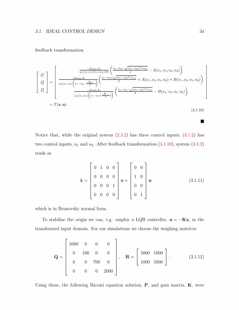
Notice that, while the original system (2.3.2) has three control inputs, (3.1.2) has
two control inputs, u1 and u2. After feedback transformation (3.1.10), system (3.1.2)
reads as
x =
0 1 0 0
0 0 0 0
0 0 0 1
0 0 0 0
x +
0 0
1 0
0 0
0 1
u (3.1.11)
which is in Brunovsky normal form.
To stabilize the origin we can, e.g. employ a LQR controller, u = −Kx, in the
transformed input domain. For our simulations we choose the weighing matrices
Q =
5000 0 0 0
0 100 0 0
0 0 700 0
0 0 0 2000
, R =
5000 1000
1000 5000
. (3.1.12)
Using these, the following Riccati equation solution, P, and gain matrix, K, were

3.1. IDEAL CONTROL DESIGN 35
generated
P =
7065.5 4955.6 137.7 340.1
4955.6 7051.7 248.6 847.8
137.7 248.6 2002.6 1866.5
340.1 847.8 1866.5 5349.2
,
K =
1.0183 1.4338 −0.0260 −0.0463
−0.1356 −0.1172 0.3785 1.0791
.
(3.1.13)
The design of a nonlinear stabilizer in the absence of uncertainties is now complete.
Notice that tracking can also be straightforwardly achieved for system (3.1.2). Con-
troller performance for this specific application is measured in two ways, namely the
amplitude of the control input (ie. currents) and the size of the domain of attraction.
The goal is to have small currents and a large domain of attraction. The motivation
of having low currents is to avoid the magnet windings from overheating and, more
importantly, to prevent the actuators from saturating. It is not known exactly at
what current the magnet wire will overheat, however after running some tests on the
actual system, the aim is to have the current peaks below 10 A and the continuous
currents not exceed 6 A. Thus no current should be above 10 A for more then 1
second. These currents are close to the limit of our actuator but if εb1 and εb2 are
made very small, the current can be kept below this limit in most cases.
As for the second performance criterion, an estimate of the domain of attraction
of the origin of the closed-loop system can be obtained by finding the largest level set
of V contained inside the set C defined in (3.1.1), where our controller is guaranteed
to be valid. In other words we want to find the largest value of c > 0 such that
ΩC :=
x ∈ <4∣
∣
∣V (x) = xTPx ≤ c
⊂ C. (3.1.14)
3.1. IDEAL CONTROL DESIGN 36
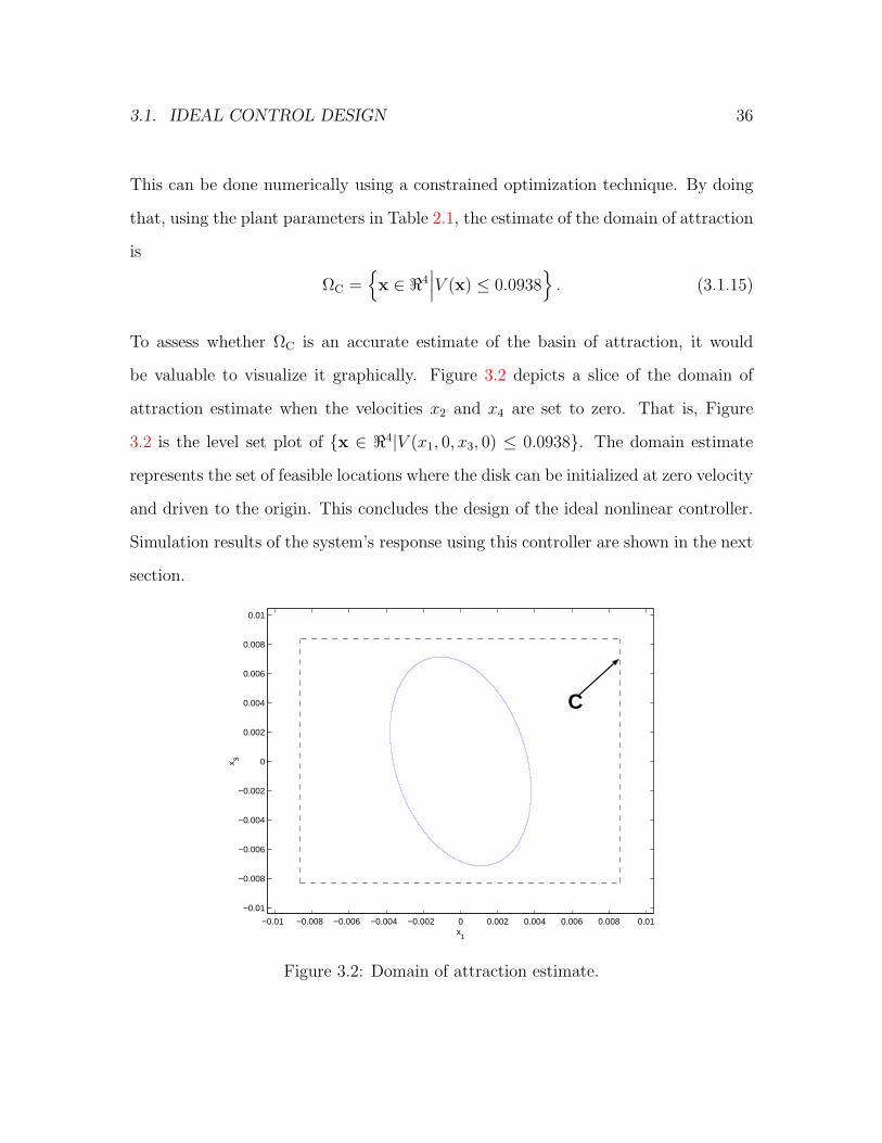
This can be done numerically using a constrained optimization technique. By doing
that, using the plant parameters in Table 2.1, the estimate of the domain of attraction
is
ΩC =
x ∈ <4∣
∣
∣V (x) ≤ 0.0938
. (3.1.15)
To assess whether ΩC is an accurate estimate of the basin of attraction, it would
be valuable to visualize it graphically. Figure 3.2 depicts a slice of the domain of
attraction estimate when the velocities x2 and x4 are set to zero. That is, Figure
3.2 is the level set plot of x ∈ <4|V (x1, 0, x3, 0) ≤ 0.0938. The domain estimate
represents the set of feasible locations where the disk can be initialized at zero velocity
and driven to the origin. This concludes the design of the ideal nonlinear controller.
Simulation results of the system’s response using this controller are shown in the next
section.
−0.01 −0.008 −0.006 −0.004 −0.002 0 0.002 0.004 0.006 0.008 0.01
−0.01
−0.008
−0.006
−0.004
−0.002
0
0.002
0.004
0.006
0.008
0.01
x1
x 3
C
Figure 3.2: Domain of attraction estimate.
3.1. IDEAL CONTROL DESIGN 37
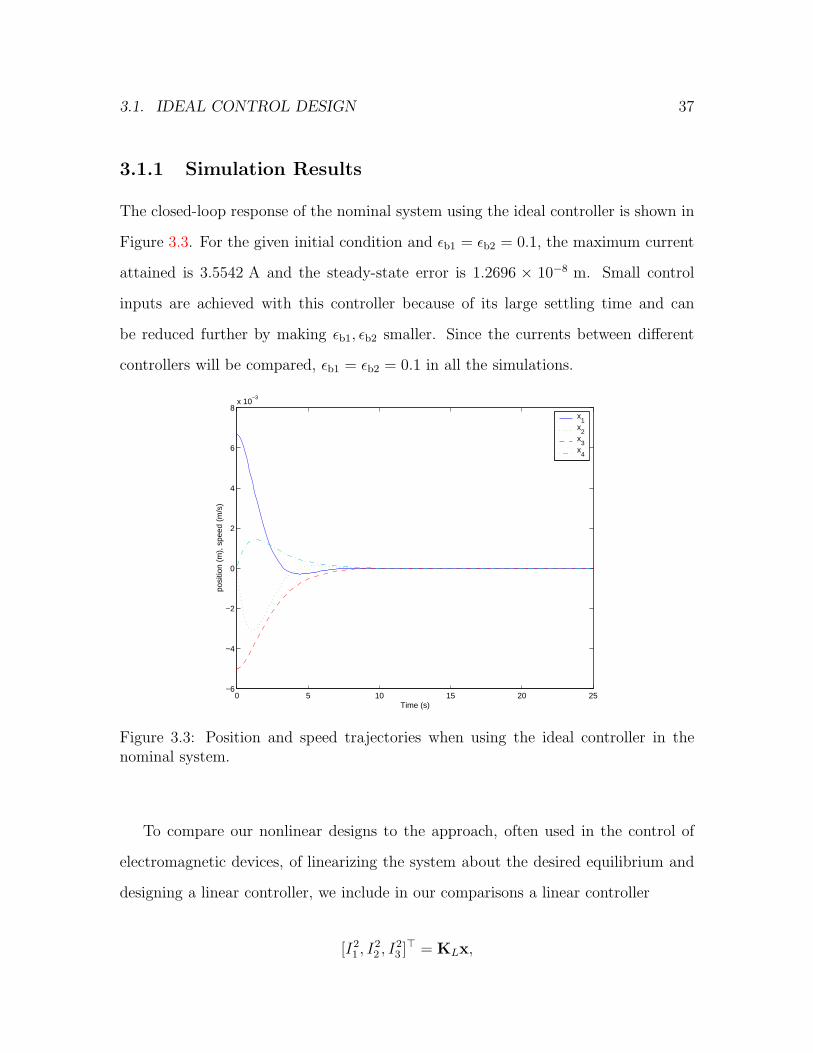
3.1.1 Simulation Results
The closed-loop response of the nominal system using the ideal controller is shown in
Figure 3.3. For the given initial condition and εb1 = εb2 = 0.1, the maximum current
attained is 3.5542 A and the steady-state error is 1.2696 × 10⁻⁸ m. Small control
inputs are achieved with this controller because of its large settling time and can
be reduced further by making εb1, εb2 smaller. Since the currents between different
controllers will be compared, εb1 = εb2 = 0.1 in all the simulations.
0 5 10 15 20 25−6
−4
−2
0
2
4
6
8x 10
−3
Time (s)
posi
tion
(m),
spe
ed (
m/s
)
x1
x2
x3
x4
Figure 3.3: Position and speed trajectories when using the ideal controller in thenominal system.
To compare our nonlinear designs to the approach, often used in the control of
electromagnetic devices, of linearizing the system about the desired equilibrium and
designing a linear controller, we include in our comparisons a linear controller
[I21 , I
22 , I
23 ]> = KLx,

3.1. IDEAL CONTROL DESIGN 38
where the matrix KL is obtained by applying LQR design to the linearization of the
system at the origin, with
Q =
5000 0 0 0
0 100 0 0
0 0 700 0
0 0 0 2000
, R =
1000 0 0
0 100 0
0 0 1000
. (3.1.16)
The projection on the (x1, x3) plane of the phase curves of the uncertainty-free
system using the linear controller and the ideal controller developed in Section 3.1 is
shown in Figure 3.4. It depicts trajectories of the controllers for five initial conditions.
The performance of the ideal and linear controllers in the uncertainty-free system is
comparable.
−0.01 −0.008 −0.006 −0.004 −0.002 0 0.002 0.004 0.006 0.008 0.01−0.01
−0.008
−0.006
−0.004
−0.002
0
0.002
0.004
0.006
0.008
0.01
x1
x 3
linear
ideal
Slice of DOA
Figure 3.4: Projection of the phase curves on the x1 − x3 plane when using the idealand linear controllers in the nominal system.
These are the only simulations on the nominal system. All other simulations
depict various controllers used in the system when uncertainties are present.

3.2. ROBUST CONTROL DESIGN 39
3.2 Robust Control Design
In this section we robustify the controller developed in the previous section to ac-
count for the uncertainties in (2.4.1). To this end, using the feedback transformation
(3.1.10), (2.4.1) is mapped to
x =
0 1 0 0
0 0 0 0
0 0 0 1
0 0 0 0
x +
0 0
1 0
0 0
0 1
(u + δ(x)) (3.2.1)
where δ(x) = [δ2(x1, x2, x3), δ4(x1, x3, x4)]>. Since the uncertainty δ(x) satisfies a
matching condition, Lyapunov redesign is a natural choice for robust stabilization.
Following the standard Lyapunov redesign technique (see, e.g., [2]), we replace the
linear controller (in the transformed input domain) developed in the previous section,
u = −Kx, by u = −Kx+v, where v is an additional control term designed to stabilize
the system subject to uncertainties. In order to do that, we use the inequalities in
(2.4.2) and assume that we know two positive scalars β1 and β2 satisfying
|θi| ≤ β1, i = 1, 2, 4, 5, |θj | ≤ β2, j = 3, 6.
Assume that with u = Ψ(x) + v an upper bound, ρ(x), to the uncertain terms exists
such that ||δ(x)|| ≤ ρ(x),
||δ(x)||2 =
√
|δ2|2 + |δ4|2
= (θ1 |x1| + θ2 |x3| − θ3x2)2 + (θ4 |x1| + θ5 |x3| − θ6x4)
2
= (θ1 |x1| + θ2 |x3|)2 − 2θ3x2 (θ1 |x1| + θ2 |x3|) − 2θ6x4 (θ4 |x1| + θ5 |x3|)
+ (θ4 |x1| + θ5 |x3|)2 + θ23x
22 + θ2
6x24
3.2. ROBUST CONTROL DESIGN 40
≤√
2β21(|x1| + |x3|)2 + 2β1β2(|x1| + |x3|)(|x2| + |x4|) + β2
2 (x22 + x2
4)
≤√
2β∗2(|x1| + |x3|)2 + 2β∗2(|x1| + |x3|)(|x2| + |x4|) + β∗2 (x22 + x2
4)
:= ρ(x)
where β∗ = max β1, β2. Next, apply u = Ψ(x) + v to (3.2.1) and perform Lyapunov
analysis
V = xT Px + xT Px
= −xTQx + 2xTPB(v + δ(x))
≤ −λmin(Q)||x||22 + ωT (v + δ(x))
≤ −λmin(Q)||x||22 + ωTv + ||ω||2||δ||2
≤ −λmin(Q)||x||22 + ωTv + ||ω||2ρ(x)
where ωT = 2xTPB, λmin(Q) denotes the minimum eigenvalue of matrix Q and
Q ∈ <2×2 is positive definite and symmetric. Choose v that renders V negative,
v = −η(x) ω||ω||2 , where η(x) ≥ ρ(x), so that
V = −λmin(Q)||x||22 −ωTω
||ω||2η(x) + ||ω||2ρ(x)
= −λmin(Q)||x||22 + ||ω||2(ρ(x) − η(x)) < 0 ∀ x ∈ <4 6= 0.
The redesign of v stabilizes the system with uncertainties. Since v is not smooth at
the origin, we replace v by the following smooth version (see [2]):
v =
−η(x) ω||ω||2 if η(x)||ω||2 ≥ γ
−η(x)2 ωγ
if η(x)||ω||2 < γ(3.2.2)
where γ > 0. The resulting closed-loop trajectories converge to a neighborhood of

3.2. ROBUST CONTROL DESIGN 41
order γ about the origin. Since γ can be made arbitrarily small, the asymptotic set-
point regulation error can be made negligible. This completes the robust nonlinear
control design. Simulation results of the robust controller are shown in the next
section.
3.2.1 Simulation Results
Introducing the first scenario for simulations:
Case 1:
δ1(x1, x2, x3) ≤ 1.1 |x1| + 0.5 |x3| − 0.01x2
δ2(x1, x3, x4) ≤ 0.5 |x1| + 1.1 |x3| − 0.01x4
x(0) =[
6.67 mm 0 −5 mm 0
]>.
All controllers are tested in this scenario. Figure 3.5 depict the x and y positions
of the ideal nonlinear controller and the robust nonlinear controller when subject to
uncertainties of case 1. The maximum upper bound of the robust controller is set to
β∗ = 1.5 and low steady-state errors are achieved by setting γ = 10−5. In this scenario,
the ideal controller fails to stabilize the system while the robust controller manages to
stabilize the system about the origin. Notice that although the robust redesign does
not guarantee performance improvement, simulations suggest that transient response
is improved with the robust controller.
Figure 3.6 show the x and y positions of the robust nonlinear controller and the LQR
controller designed from the linearized system. Figure 3.6 is the response when the
uncertainties defined in case 1 are present. The linear controller, although robust
about the point, is unable to stabilize the system in this first scenario. As before, the
3.2. ROBUST CONTROL DESIGN 42
0 5 10 15 20 25−0.01
−0.005
0
0.005
0.01
0.015
0.02
Time (s)
x po
sitio
n (m
)
0 5 10 15 20 25−0.01
−0.005
0
0.005
0.01
0.015
0.02
Time (s)
y po
sitio
n (m
)
ideal
robust
robust
ideal
Figure 3.5: Case 1 response of uncertain system when using ideal and robust nonlinearcontrollers.
robust nonlinear controller successfully stabilizes the system with reasonable perfor-
mance.
In case 1, the robust controller achieves a steady-state error of 9.4459 × 10⁻⁶ m
at a maximum current of 3.7079 A using εb1 = εb2 = 0.1 . The currents of the
robust controller are depicted in Figure 3.7. Although these results indicate that
the robust controller can compensate for large uncertainties while maintaining high
performance, there are some practical issues with using this controller, namely the
chattering effect of the control inputs seen in Figure 3.7 that can excite high-frequency
un-modelled dynamics in the system [9]. Further, these currents are impossible to
obtain in practice because they are too high-frequency.

3.2. ROBUST CONTROL DESIGN 43
0 5 10 15 20 25−5
0
5
10
15x 10
−3
Time (s)
x po
sitio
n (m
)
0 5 10 15 20 25−0.01
−0.005
0
0.005
0.01
Time (s)
y po
sitio
n (m
)linear
robust
linear
robust
Figure 3.6: Case 1 response of uncertain system when using a linear controller andthe robust nonlinear controller.
0 2 4 6 8 10 12 14 16 18 202.5
3
3.5
4
Time (s)
Cur
rent
(A
)
I3
I1
I2
Figure 3.7: Currents of robust nonlinear controller in system subject to case 1.

3.3. ADAPTIVE CONTROL DESIGN 44
3.3 Adaptive Control Design
Although the robust controller developed in the previous section guarantees stability
for the system subject to uncertainties δ2 and δ4 in (2.4.1), it does have practical
drawbacks. Specifically, as shown in Section 3.2.1, the currents have a high-frequency
component due to the fact that (3.2.2) is the smooth version of a sliding mode con-
troller. Further, a robust controller may require a large control effort which is not
desirable in the application under consideration because of the saturation limits of
the amplifiers. Both drawbacks above may, in principle, be overcome by designing an
adaptive controller. Thus, assuming that the structure of the uncertainties in (2.4.1)
is known exactly, which is not a realistic assumption, a nonlinear adaptive controller
is designed. The set-point adaptive regulation methodology we employ here is found
in [4] and, depending on the size of the uncertainties, can give an overall better re-
sponse with considerably less control effort. In what follows, we present the control
design procedure and simulation results comparing the performance of the adaptive
control to that of the robust controller.
3.3.1 Backstepping Design
The adaptive regulation presented in [4] globally stabilizes an equilibrium point and
regulates a set-point for a strict-parametric system. A strict-parametric system with
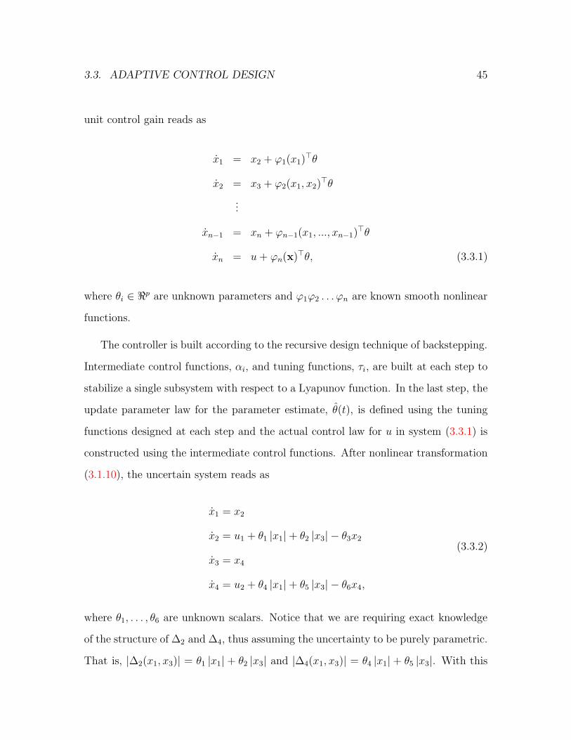
3.3. ADAPTIVE CONTROL DESIGN 45
unit control gain reads as
x1 = x2 + ϕ1(x1)>θ
x2 = x3 + ϕ2(x1, x2)>θ
...
xn−1 = xn + ϕn−1(x1, ..., xn−1)>θ
xn = u+ ϕn(x)>θ, (3.3.1)
where θi ∈ <p are unknown parameters and ϕ1ϕ2 . . . ϕn are known smooth nonlinear
functions.
The controller is built according to the recursive design technique of backstepping.
Intermediate control functions, αi, and tuning functions, τi, are built at each step to
stabilize a single subsystem with respect to a Lyapunov function. In the last step, the
update parameter law for the parameter estimate, θ(t), is defined using the tuning
functions designed at each step and the actual control law for u in system (3.3.1) is
constructed using the intermediate control functions. After nonlinear transformation
(3.1.10), the uncertain system reads as
x1 = x2
x2 = u1 + θ1 |x1| + θ2 |x3| − θ3x2
x3 = x4
x4 = u2 + θ4 |x1| + θ5 |x3| − θ6x4,
(3.3.2)
where θ1, . . . , θ6 are unknown scalars. Notice that we are requiring exact knowledge
of the structure of ∆2 and ∆4, thus assuming the uncertainty to be purely parametric.
That is, |∆2(x1, x3)| = θ1 |x1| + θ2 |x3| and |∆4(x1, x3)| = θ4 |x1| + θ5 |x3|. With this

3.3. ADAPTIVE CONTROL DESIGN 46
in mind, notice that (3.3.2) matches the strict-parametric system (3.3.1) by letting
u1 := x3
ϕ1 := 0
ϕ2 :=[
|x1| −x2 0 0 0]>
ϕ3 := 0
ϕ4 :=[
0 0 |x1| |x3| −x4
]>
θ :=[
θ1 θ3 θ4 θ5 θ6
]>. (3.3.3)
Remark 3.3.1. The transformed system (3.3.2) is not decoupled because the uncer-
tainty entering u1 and u2 depends on both positions, x1 and x3. Thus the adaptive
scheme cannot be applied to the (x1, x2) subsystem, and to the (x3, x4) subsystem
individually. To avoid this problem we set u1 = x3 and stabilize the entire system
using only u2.
Remark 3.3.2. The adaptive control is based on stabilizing an uncertain system in
strict-parametric form and therefore it cannot compensate for the θ2 |x3| term in
(3.3.2). As shown in the simulations later, the adaptive control is unable to stabilize
the system if this term is too large.
Step 1. In the first step, the error states are
z1 = x1
z2 = x2 − α1,
3.3. ADAPTIVE CONTROL DESIGN 47
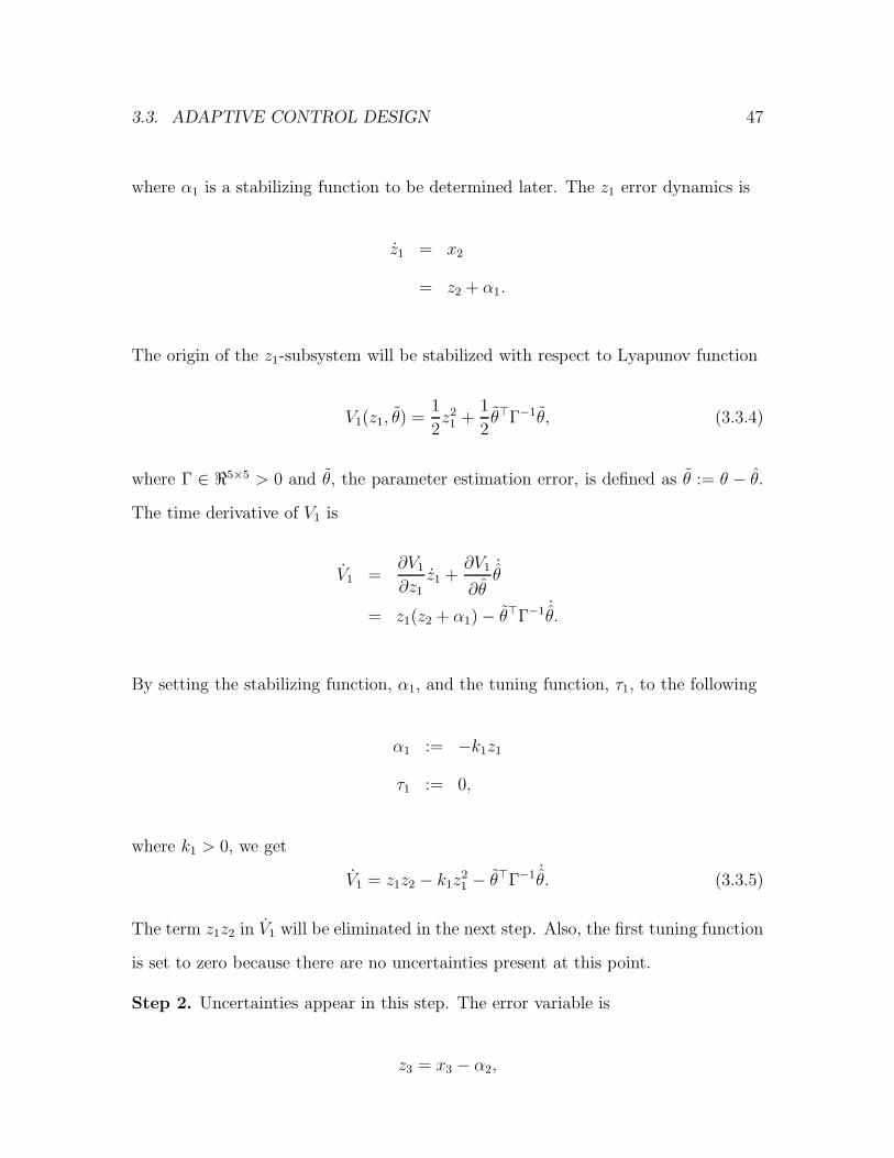
where α1 is a stabilizing function to be determined later. The z1 error dynamics is
z1 = x2
= z2 + α1.
The origin of the z1-subsystem will be stabilized with respect to Lyapunov function
V1(z1, θ) =1
2z21 +
1
2θ>Γ−1θ, (3.3.4)
where Γ ∈ <5×5 > 0 and θ, the parameter estimation error, is defined as θ := θ − θ.
The time derivative of V1 is
V1 =∂V1
∂z1z1 +
∂V1
∂θ
˙θ
= z1(z2 + α1) − θ>Γ−1 ˙θ.
By setting the stabilizing function, α1, and the tuning function, τ1, to the following
α1 := −k1z1
τ1 := 0,
where k1 > 0, we get
V1 = z1z2 − k1z21 − θ>Γ−1 ˙
θ. (3.3.5)
The term z1z2 in V1 will be eliminated in the next step. Also, the first tuning function
is set to zero because there are no uncertainties present at this point.
Step 2. Uncertainties appear in this step. The error variable is
z3 = x3 − α2,

3.3. ADAPTIVE CONTROL DESIGN 48
where α2 is a stabilizing function to be determined later. The (z1, z2)-dynamics are
then given by
z1 = z2 + α1
z2 =∂z2
∂x1
x1 +∂z2
∂x2
x2 +∂z2
∂θ
˙θ
= −∂α1
∂x1x2 + z3 + α2 + ϕ>
2 θ.
Define the Lyapunov function in the second step as,
V2(z1, z2, θ) = V1 +1
2z22 . (3.3.6)
Taking the derivative of V2 along solutions z1, z2 and˙θ gives
V2 = V1 + z2z2
= z1z2 − k1z21 − θ>Γ−1 ˙
θ + z2
(
−∂α1
∂x1x2 + z3 + α2 + ϕ>
2 θ
)
.
The stabilizing function, α2, and the tuning function, τ2, are chosen so that if z3 = 0
and Γ−1 ˆθ = τ2, V2 is negative semi-definite
α2 := −z1 − k2z2 +∂α1
∂x1x2 − ϕ>
2 θ
τ2 := ϕ2z2,
where k2 > 0. The Lyapunov derivative then becomes
V2 = z2z3 − k1z21 − k2z
22 + z2ϕ
>2 (θ − θ) − θ>Γ−1 ˙
θ
= z2z3 − k1z21 − k2z
22 + θ>(ϕ2z2 − Γ−1 ˙
θ)
= z2z3 − k1z21 − k2z
22 + θ>
(
τ2 − Γ−1 ˙θ)
.
3.3. ADAPTIVE CONTROL DESIGN 49
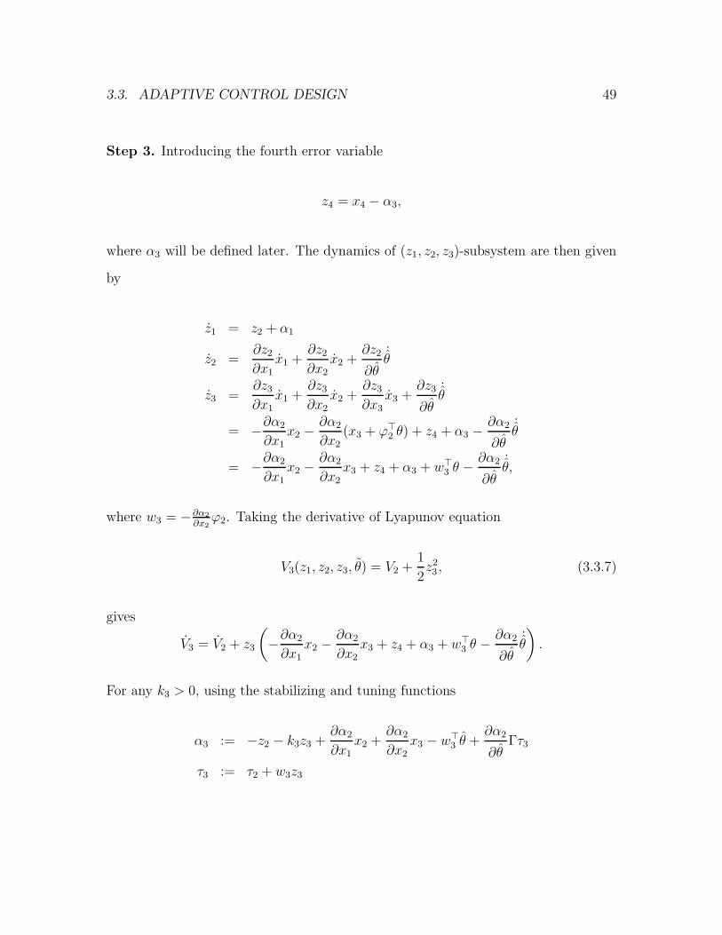
Step 3. Introducing the fourth error variable
z4 = x4 − α3,
where α3 will be defined later. The dynamics of (z1, z2, z3)-subsystem are then given
by
z1 = z2 + α1
z2 =∂z2
∂x1
x1 +∂z2
∂x2
x2 +∂z2
∂θ
˙θ
z3 =∂z3
∂x1x1 +
∂z3
∂x2x2 +
∂z3
∂x3x3 +
∂z3
∂θ
˙θ
= −∂α2
∂x1x2 −
∂α2
∂x2(x3 + ϕ>
2 θ) + z4 + α3 −∂α2
∂θ
˙θ
= −∂α2
∂x1
x2 −∂α2
∂x2
x3 + z4 + α3 + w>3 θ −
∂α2
∂θ
˙θ,
where w3 = −∂α2
∂x2ϕ2. Taking the derivative of Lyapunov equation
V3(z1, z2, z3, θ) = V2 +1
2z23 , (3.3.7)
gives
V3 = V2 + z3
(
−∂α2
∂x1x2 −
∂α2
∂x2x3 + z4 + α3 + w>
3 θ −∂α2
∂θ
˙θ
)
.
For any k3 > 0, using the stabilizing and tuning functions
α3 := −z2 − k3z3 +∂α2
∂x1x2 +
∂α2
∂x2x3 − w>
3 θ +∂α2
∂θΓτ3
τ3 := τ2 + w3z3

3.3. ADAPTIVE CONTROL DESIGN 50
gives the Lyapunov function derivative
V3 = z3z4 − k1z21 − k2z
22 − k3z
23 + θ>
(
τ2 − Γ−1 ˙θ)
+ z3w>3 θ + z3
∂α2
∂θΓ(
τ3 − Γ−1 ˙θ)
= z3z4 − k1z21 − k2z
22 − k3z
23 + θ>
(
τ2 + z3w3 − Γ−1 ˙θ)
+ z3∂α2
∂θΓ(
τ3 − Γ−1 ˙θ)
= z3z4 − k1z21 − k2z
22 − k3z
23 +
(
θ> + z3∂α2
∂θΓ
)
(
τ3 − Γ−1 ˙θ)
.
Step 4. In the final step, the parameter estimate update law is finalized and the
control law entering u2 in (3.3.2) is built using the previous stabilizing functions.
The final Lyapunov function is
V4 = V3 +1
2z24 ,
where z4 is the error variable defined in the step 3. The complete error dynamics are
z1 = z2 + α1
z2 =∂z2
∂x1
x1 +∂z2
∂x2
x2 +∂z2
∂θ
˙θ
z3 =∂z3
∂x1x1 +
∂z3
∂x2x2 +
∂z3
∂x3x3 +
∂z3
∂θ
˙θ
z4 =∂z4
∂x1x1 +
∂z4
∂x2x2 +
∂z4
∂x3x3 +
∂z4
∂x4x4 +
∂z4
∂θ
˙θ
= −∂α3
∂x1x2 −
∂α3
∂x2(x3 + ϕ>
2 θ) −∂α3
∂x3x4 + u2 + ϕ>
4 θ −∂α3
∂θ
˙θ
= −∂α3
∂x1
x2 −∂α3
∂x2
x3 −∂α3
∂x3
x4 + u2 +
[
ϕ>4 − ∂α3
∂x2
ϕ>2
]
θ − ∂α3
∂θ
˙θ
= −∂α3
∂x1x2 −
∂α3
∂x2x3 −
∂α3
∂x3x4 + u2 + w>
4 θ −∂α3
∂θ
˙θ,
where w4 = ϕ4 − ∂α3
∂x2ϕ2. Taking the derivative of V4 along solutions gives
V4 = V3 + z4
(
−∂α3
∂x1x2 −
∂α3
∂x2x3 −
∂α3
∂x3x4 + u2 + w>
4 θ −∂α3
∂θ
˙θ
)
.
3.3. ADAPTIVE CONTROL DESIGN 51
The final control law, u2, and the parameter update law,˙θ, can now be defined to
stabilize (z, θ), where z :=[
z1 z2 z3 z4
]>, with respect to V4
u2 := −z3 − k4z4 +∂α3
∂x1x2 +
∂α3
∂x2x3 +
∂α3
∂x3x4 +
∂α3
∂θ
˙θ − w>
4 θ
+z3∂α2
∂θΓw4
τ4 := τ3 + w4z4
˙θ := Γτ4 = Γ
[
ϕ2z2 −∂α2
∂x2z3 +
(
ϕ4 −∂α3
∂x2ϕ2
)
z4
]
.
Applying the control law, update law, and tuning function just defined to V4 gives
V4 = −k1z21 − k2z
22 − k2
3z23 − k4z
24 +
(
θ> + z3∂α2
∂θΓ
)
(
τ3 − Γ−1 ˙θ)
+z3∂α2
∂θΓw4z4 + z4w
>4 θ
= −k1z21 − k2z
22 − k2
3z23 − k4z
24 +
(
θ> + z3∂α2
∂θΓ
)
(
τ3 − Γ−1 ˙θ)
+
(
θ> + z3∂α2
∂θΓ
)
w4z4
= −k1z21 − k2z
22 − k2
3z23 − k4z
24 +
(
θ> + z3∂α2
∂θΓ
)
(
τ4 − Γ−1 ˙θ)
= −k1z21 − k2z
22 − k2
3z23 − k4z
24 . (3.3.8)
Thus V4 is negative semidefinite and, by LaSalle’s theorem, trajectories (z(t), θ(t))
converge to the largest invariant set, M, inside
E =
(z, θ) ∈ <9
∣
∣
∣
∣
z = 0
. (3.3.9)
This means that z(t) → 0 as t → ∞ and from this we can find the set M. By
substituting the stabilizing functions α1, α2, α3, and α4 into z1, z2, z3 and z4, the
3.3. ADAPTIVE CONTROL DESIGN 52
closed-loop error dynamics can be represented in matrix form
z =
−k1 1 0 0
−1 −k2 1 0
0 −1 −k3 1 + ϕ>2 Γw4
0 0 −1 −k4
z +
0 0 0 0
0 1 0 0
0 −∂α2
∂x20 0
0 ∂α3
∂x20 −1
ϕ>1
ϕ>2
ϕ>3
ϕ>4
θ.
Since z = 0 and therefore z = 0, the following system of equations arise
0 0 0 0
0 1 0 0
0 −∂α2
∂x20 0
0 ∂α3
∂x20 −1
ϕ>1
ϕ>2
ϕ>3
ϕ>4
θ = 0,
where it can be concluded that ϕ>2 θ = 0 and ϕ>
4 θ = 0. Using this result, the error
states become
x1 = 0
x2 = z2 + α1(z1, θ) = 0 + α1(0, θ) = 0
x3 = α2(0, 0, θ) = −ϕ>2 θ = 0
x4 = α3(0, 0, 0, θ) = −∂α2
∂x2ϕ2θ = 0.
The largest invariant set contained in (3.3.9) is
E =
(x, θ) ∈ <9
∣
∣
∣
∣
x = 0, ϕ>2 θ = ϕ>
2 θ, ϕ>4 θ = ϕ>
4 θ
. (3.3.10)
In conclusion, the closed-loop adaptive system is globally stable at equilibrium point
(x, θ) = (0, θ) and is set-point regulated, x(t) → 0 as t → ∞. Notice however that

3.3. ADAPTIVE CONTROL DESIGN 53
the equilibrium point is not globally asymptotically stable because the parameter
estimates do not converge to the actual parameters. The reader is referred to [4] for
more information on stability results.
3.3.2 Simulations Results
Figure 3.8 shows the closed-loop system response when using the adaptive controller
in the first scenario. The adaptive control design parameters are: k1 = 2, k2 = 3.5,
k3 = 2, k4 = 3.5, θ(0) =[
0 0 0 0 0
]>and Γ = diag
[
3, 3, 3, 3, 3
]
.
As shown in Figure 3.8, the adaptive control fails to handle the uncertainties in case
1. The adaptive controller is unable to stabilize the system under conditions of case
1 because the term 0.5 |x3| in δ2 is not handled by the adaptive scheme.
0 0.5 1 1.5 2 2.5 3 3.5 4 4.5 50
0.005
0.01
0.015
Time (s)
x po
sitio
n (m
)
0 0.5 1 1.5 2 2.5 3 3.5 4 4.5 5−0.01
−0.008
−0.006
−0.004
−0.002
0
Time (s)
y po
sitio
n (m
)
Figure 3.8: Case 1 response of uncertain system when using adaptive nonlinear con-trollers.
The adaptive will now be tested with uncertainties that it can fully compensate
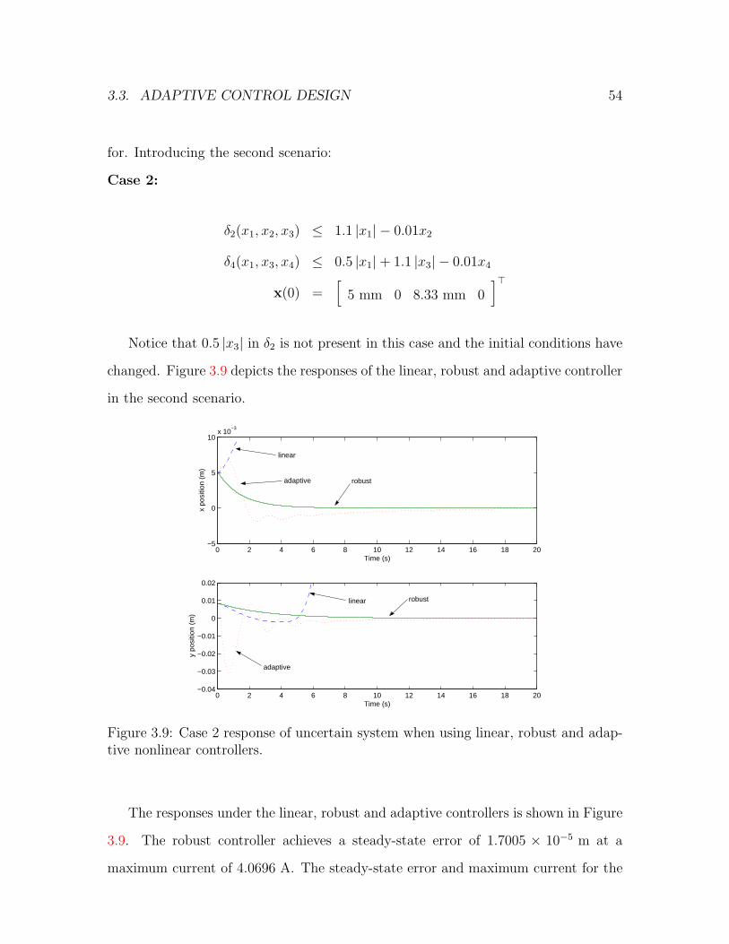
3.3. ADAPTIVE CONTROL DESIGN 54
for. Introducing the second scenario:
Case 2:
δ2(x1, x2, x3) ≤ 1.1 |x1| − 0.01x2
δ4(x1, x3, x4) ≤ 0.5 |x1| + 1.1 |x3| − 0.01x4
x(0) =[
5 mm 0 8.33 mm 0
]>
Notice that 0.5 |x3| in δ2 is not present in this case and the initial conditions have
changed. Figure 3.9 depicts the responses of the linear, robust and adaptive controller
in the second scenario.
0 2 4 6 8 10 12 14 16 18 20−5
0
5
10x 10
−3
Time (s)
x po
sitio
n (m
)
0 2 4 6 8 10 12 14 16 18 20−0.04
−0.03
−0.02
−0.01
0
0.01
0.02
Time (s)
y po
sitio
n (m
)
linear
adaptive robust
linear robust
adaptive
Figure 3.9: Case 2 response of uncertain system when using linear, robust and adap-tive nonlinear controllers.
The responses under the linear, robust and adaptive controllers is shown in Figure
3.9. The robust controller achieves a steady-state error of 1.7005 × 10⁻⁵ m at a
maximum current of 4.0696 A. The steady-state error and maximum current for the

3.3. ADAPTIVE CONTROL DESIGN 55
adaptive controller are 2.5163×10⁻⁴ m and 6.3447 A. Control inputs of the adaptive
controller are shown in Figure 3.10. The adaptive controller does not out-perform the
robust controller but, unlike the linear controller, manages to stabilize the system.
The adaptive controller does, however, calculate currents that do not chatter like
those from the robust control system. From a practical viewpoint, the hardware can
provide smooth currents from the adaptive controller but the high-frequency currents
from the robust controller cannot be realized.
0 2 4 6 8 10 12 14 16 18 201
2
3
4
5
6
7
Time (s)
Cur
rent
(A
)
I3
I2
I1
Figure 3.10: Control input of adaptive controller in case 2.
Remark 3.3.3. Note that the x3 trajectory using the adaptive controller in Figure 3.9
goes outside the domain C defined in (3.1.1) where our controller is valid. However, in
this particular response the signs of the denominators x1 +x3 +d and x1−x3 +√
3−12d
in (3.1.5) are still positive and the expression x1 − x3 −√
3+12d in the denominator
of I2 is still negative. In simulation it occurs that the trajectories go outside C but
rarely does the control become undefined. This shows that domain C is somewhat
conservative.

3.3. ADAPTIVE CONTROL DESIGN 56
It was found that the adaptive control system performs very well with low currents
when uncertainties ∆2 and ∆4 are in the lower range. It was also observed that the
adaptive controller performs even better when the frictions applied to the system
are high. Thus, the hypothesis of a better performance and control effort tradeoff is
confirmed through simulation for lighter uncertainties.
The adaptive control cannot be used in the actual system because in practice
the functional forms of the uncertainties are not known. Thus both the robust (be-
cause of the chattering) and the adaptive controllers cannot be used if the simulated
uncertainties in case 1 or 2 are large (and therefore realistic).

3.4. ROBUST ADAPTIVE CONTROL DESIGN 57
3.4 Robust Adaptive Control Design
The tradeoff between control effort and steady-state error is only improved with the
adaptive controller if the uncertainties present in the system are small. Further,
the adaptive control requires the uncertainties in (2.4.1) to be structured, i.e., to
exactly match the structure the adaptive control design calls for, and to be linear with
respect to unknown parameters. Uncertainties δ2 and δ4 in (2.4.2) cannot be assumed
to be structured and to be linear functions of unknown parameters (although, this
assumption is reasonable for the viscous friction terms). In the light of the above,
we choose to develop a robust adaptive control that handles friction in the classic
adaptive manner but compensates uncertainties ∆2 and ∆4 in (2.4.2) using adaptive
upper bounds. Thus, even if the uncertainty of the model assumptions outlined in
Chapter 2 do not match the strict-parametric structure in the adaptive controller,
the system can still be stabilized. To this end, we employ the methodology developed
in [6]. The robust adaptive controller enjoys better performance than the robust and
adaptive controllers at the expense of high peak currents. Simulations that compare
these controllers will be shown after the control design is illustrated.
3.4.1 Backstepping Design
We employ the technique developed by Polycarpou and Iannou in [6], which en-
sures that the trajectories of the closed-loop system are globally uniformly ultimately
bounded (GUUB) with a small ultimate bound. The methodology in [6] applies to
the class of nonlinear systems that satisfy the triangular bounds condition. Consider
the following n-dimensional single-input nonlinear system
xi = xi+1 + θ>ϕi(x1, ..., xi) + ∆i(x, t), 1 ≤ i ≤ n− 1
xn = u+ θ>ϕn(x) + ∆n(x, t),(3.4.1)
3.4. ROBUST ADAPTIVE CONTROL DESIGN 58
where θ1, . . . , θn are unknown scalar parameters, ϕ1, . . . , ϕn are known smooth func-
tions and ∆1, . . . ,∆n are unknown functions that satisfy Assumption 3.4.1.
Assumption 3.4.1. There exists, possibly unknown, parameters ψi ∈ < ≥ 0 and
known smooth functions pi : <i → <+\0 such that for all x ∈ <n and t ∈ <+
|∆i(x, t)| ≤ ψipi(x1, ..., xi), 1 ≤ i ≤ n. (3.4.2)
Recall that, after applying the nonlinear input transformation (3.1.10) to the uncer-
tain system (2.4.1), we get
x1 = x2
x2 = u1 +δ2(x1, x2, x3)
m
x3 = x4
x4 = u2 +δ4(x1, x3, x4)
m.
(3.4.3)
Recalling, from (2.4.2), that
δ2(x) = ∆2(x1, x3) − θ3x2,
δ4(x) = ∆4(x1, x3) − θ6x4,
where ∆2(x1, x3) ≤ θ1|x1| + θ2|x3| and ∆4(x1, x3) ≤ θ4|x1| + θ5|x3|, and letting
u1 := x3
ϕ1 :=[
0 0 0 0
]>
ϕ2 :=[
0 −x2 0 0]>

3.4. ROBUST ADAPTIVE CONTROL DESIGN 59
ϕ3 :=[
0 0 0 0
]>
ϕ4 :=[
0 0 0 −x4
]>,
we have that (3.4.3) fits the structure in (3.4.1). Next, in order for condition (3.4.1)
to be satisfied we need to impose the requirement that θ2 = 0, and we need to find
a smooth upper bound to |∆2(x1, x3)| (the function θ2|x3| is not smooth). Noticing
that for any c1, c2 > 0, there exist scalars ψ2, ψ4 > 0 such that
θ1|x1| ≤ ψ2(x21 + c1),
θ4|x1| + θ5|x3| ≤ ψ4(|x1| + |x3| + c2),
and setting
p2(x1) = x21 + c1 (3.4.4)
p4(x1, x3) = |x1| + |x3| + c2, (3.4.5)
we have that (3.4.1) is satisfied. The imposed requirement that θ2 = 0 (i.e. that ∆2
be independent of x3) poses a limitation to the generality of the solution presented
here. The impact of this requirement on the performance of the experimental testbed
under construction will be the subject of future investigation in other research.
Similarly to the adaptive control design, the robust adaptive controller is con-
structed using the backstepping technique. At each step we define an error variable
zi, an intermediate feedback control, αi, a tuning function, τi, and a update law,
˙Ψ, made to stabilize the (z1, . . . , zi) subsystem, for i = 1, . . . , n, with respect to a
Lyapunov function Vi. The intermediate feedback controls are used to define the final

3.4. ROBUST ADAPTIVE CONTROL DESIGN 60
control u2 in system (3.4.3), while the tuning functions are used to construct the pa-
rameter update law˙θ that estimates the coefficients of friction. The final control law,
u2, employs these parameter estimates to compensate for the effect of friction. The
robust adaptive controller includes an additional update law,˙Ψi, that compensates
the effects of ∆i. This law updates the parameter estimates, Ψi, that multiply the
upper bounds pi defined in (3.4.1). In effect, the control law uses the upper bound
estimates generated by this update law to handle the effects of uncertainties caused
by various electromagnetic modelling assumptions not holding.
Step 1. The error variables are
z1 = x1
z2 = x2 − α1,
and the z1-dynamics are
z1 = x2 = z2 + α1,
where α1 is a stabilizing function that is yet to be defined. The z1 system will be
stabilized with respect to V1, defined as
V1(z1, θ, ψ1) =1
2z21 +
1
2θ>Γ−1θ +
1
2γ1
ψ21 (3.4.6)
where θ = θ(t) − θ, ψ1 = ψ1(t) − ψ1, Γ ∈ <4×4 > 0 and γ1 > 0. The time derivative
of V1 is
V1 =∂V1
∂z1z1 +
∂V1
∂θ
˙θ +
∂V1
∂ψ
˙ψ
= z1(z2 + α1) + θ>Γ−1(˙θ − τ1) + θ>Γ−1τ1 +
1
γ1ψ1
˙ψ1(t).
3.4. ROBUST ADAPTIVE CONTROL DESIGN 61
For z1 and z2 to be stabilized with respect to V1, set α1, τ1 and˙ψ1 to
α1 := −k1z1
τ1 := −σθΓ(θ − θ0)
˙ψ1(t) := −σ1γ1(ψ1 − ψ0
1)
where k1, σθ, σ1, > 0 and θ0, ψ01 ≥ 0. Thus
V1 = z1z2 − k1z21 + θ>Γ−1(
˙θ − τ1) − σθθ
>(θ − θ0) − σ1ψ1(ψ1 − ψ01).
By completing the squares, the two last terms in the previous expression are written
as
−σθ θ>(θ − θ0) = −1
2σθθ
>θ − 1
2σθ
∣
∣
∣θ − θ0
∣
∣
∣
2
+1
2σθ
∣
∣θ − θ0∣
∣
2
−σ1ψ1(ψ1 − ψ01) = −1
2σ1ψ
21 −
1
2σ1(ψ1 − ψ0
1)2 +
1
2σ1(ψ
M1 − ψ0
1)2
where ψM1 = maxψ1, ψ
01. Using these equalities we obtain
V1 = z1z2 − k1z21 + θ>Γ−1(
˙θ − τ1) −
1
2σθ θ
>θ − 1
2σθ
∣
∣
∣θ − θ0
∣
∣
∣
2
+1
2σθ
∣
∣θ − θ0∣
∣
2
−1
2σ1ψ
21 −
1
2σ1(ψ1 − ψ0
1)2 +
1
2σ1(ψ
M1 − ψ0
1)2
≤ z1z2 − k1z21 −
1
2σθθ
>θ − 1
2σ1ψ
21 + θ>Γ−1(
˙θ − τ1) +
1
2σθ
∣
∣θ − θ0∣
∣
2
+1
2σ1(ψ
M1 − ψ0
1)2
≤ z1z2 − c1V1 + λ1 + θ>Γ−1(˙θ − τ1)
where
c1 := min
2k1, σ1γ1,σθ
λmin(Γ−1)
> 0
3.4. ROBUST ADAPTIVE CONTROL DESIGN 62
λ1 :=1
2σθ
∣
∣θ − θ0∣
∣
2+
1
2σ1(ψ
M1 − ψ0
1)2.
Step 2. The new error variable is
z3 = x3 − α2,
where α2 is a stabilizing function to be chosen later. The error dynamics of the
(z1, z2)-subsystem are
z1 = z2 + α1
z2 =∂z2
∂x1
x1 +∂z2
∂x2
x2 +∂z2
∂θ
˙θ +
∂z2
∂ψ2
˙ψ2
= −∂α1
∂x1x2 + x3 + δ2
= −∂α1
∂x1x2 + z3 + α2 + θ>ϕ2 + ∆2.
Using the function
V2(z1, z2, θ, ψ1, ψ2) = V1 +1
2z22 +
1
2γ2ψ2
2,
where γ2 > 0 and for ψM2 = max
ψ2, ψo2
, ψ2 := ψ2 − ψM2 , we can find an α2, τ2 and
˙ψ2 such that the (z1, z2) subsystem is stabilized. The derivative of V2 gives
V2 = V1 + z2z2 +1
γ2ψ2
˙ψ2
= V1 + z2
[
−∂α1
∂x1x2 + z3 + α2 + θ>ϕ2 + ∆2
]
+1
γ2ψ2
˙ψ2
≤ z1z2 − c1V1 + λ1 + θ>Γ−1(˙θ − τ1)
+z2
[
−∂α1
∂x1x2 + z3 + α2 + θ>ϕ2
]
+ z2ψM2 p2 +
1
γ2ψ2
˙ψ2.

3.4. ROBUST ADAPTIVE CONTROL DESIGN 63
For ε2, σ2 > 0 and ψ02 ≥ 0, set
α2 := −z1 − k2z2 +∂α1
∂x1
x2 − θ>ϕ2 − ψ2ω2
τ2 := τ1 + Γz2ϕ2
˙ψ2(t) := γ2
(
z2ω2 − σ2(ψ2 − ψ02))
ω2 := p2 tanh
[
z2p2
ε2
]
.
Applying intermediate control law α2, tuning function τ2 and parameter update law
˙ψ2(t) to V2 gives
V2 ≤ z2z3 − c1V1 − k2z22 + λ1 + θ>Γ−1(
˙θ − τ1) − z2θ
>ϕ2 + z2ψM2 p2 − z2ψ2ω2
+z2ψ2ω2 − σ2ψ2(ψ2 − ψ02)
= z2z3 − c1V1 − k2z22 + λ1 + θ>Γ−1(
˙θ − τ1) − z2θ
>ϕ2 + z2ψM2 p2 − z2ψ2ω2
+z2(ψ2 − ψM2 )ω2 − σ2ψ2(ψ2 − ψ0
2)
= z2z3 − c1V1 − k2z22 + λ1 + θ>Γ−1(
˙θ − τ1) − z2θ
>ϕ2 + z2ψM2 p2 − z2ψ
M2 ω2 −
σ2ψ2(ψ2 − ψ02)
≤ z2z3 − c1V1 − k2z22 + λ1 + θ>Γ−1(
˙θ − τ1) − z2θ
>ϕ2 + ψM2 (|z2|p2 − z2ω2) −
σ2ψ2(ψ2 − ψ02)
The Lyapunov analysis continues with some simplifications and various inequalities.
In this case term, −z2θ>φ2 is combined with θ>Γ−1(˙θ − τ1) to give θ>Γ−1(
˙θ − τ2).
Completing the squares, the last term becomes
−σ2ψ2(ψ2 − ψ02) = −1
2σ2ψ2
2 − 1
2σ2(ψ2 − ψ0
2)2 +
1
2σ2(ψ
M2 − ψ0
2)2,
3.4. ROBUST ADAPTIVE CONTROL DESIGN 64
yielding
V2 ≤ z2z3 − c1V1 − k2z22 −
1
2σ2ψ2
2+ λ1 + θ>Γ−1(
˙θ − τ2) + ψM
2 (z2p2 − z2ω2)
−1
2σ2(ψ2 − ψ0
2)2 +
1
2σ2(ψ
M2 − ψ0
2)2
≤ z2z3 − c1V1 − k2z22 −
1
2σ2ψ2
2+ λ1 + θ>Γ−1(
˙θ − τ2) + ψM
2 (z2p2 − z2ω2)
+1
2σ2(ψ
M2 − ψ0
2)2.
Using the following inequality introduced in [6]
0 ≤ |u| − u tanh(u
ε
)
≤ δε ≤ 1
2ε,
where δ = e−(δ+1) = 0.2785, ε > 0 and u ∈ <, we obtain
ψM2
(
|z2|p2 − z2p2 tanh
[
z2p2
ε2
])
≤ δψM2 ε2 ≤
1
2ψM
2 ε2.
The Lyapunov derivative then becomes
V2 ≤ z2z3 − c1V1 − k2z22 −
1
2σ2ψ2
2+ λ1 +
1
2ψM
2 ε2 +1
2σ2(ψ
M2 − ψ0
2)2 +
θ>Γ−1(˙θ − τ2)
≤ z2z3 + −c2V2 + λ2 + θ>Γ−1(˙θ − τ2)
where
c2 := min
2k1, 2k2, σ1γ1, σ2γ2,σθ
λmin(Γ−1)
> 0,
λ2 :=1
2ψM
2 ε2 +1
2σθ
∣
∣θ − θ0∣
∣
2+
1
2σ1(ψ
M1 − ψ0
1)2 +
1
2σ2(ψ
M2 − ψ0
2)2.

3.4. ROBUST ADAPTIVE CONTROL DESIGN 65
Step 3. Consider the error variable
z4 = x4 − α3,
and the error dynamics of the (z1, z2, z3)-subsystem given by
z1 = z2 + α1
z2 = −∂α1
∂x1x2 + z3 + α2 + θ>ϕ2 + ∆2
z3 =∂z3
∂x1x1 +
∂z3
∂x2x2 +
∂z3
∂x3x3 +
∂z3
∂θ
˙θ +
∂z3
∂ψ1
˙ψ1 +
∂z3
∂ψ2
˙ψ2
= −∂α2
∂x1x2 −
∂α2
∂x2(x3 + θ>ϕ2 + ∆2) + x4 −
∂α2
∂θ
˙θ − ∂α2
∂ψ1
˙ψ1 −
∂α2
∂ψ2
˙ψ2
= −∂α2
∂x1
x2 −∂α2
∂x2
x3 + z4 + α3 −∂α2
∂x2
θ>ϕ2 −∂α2
∂x2
∆2 −∂α2
∂θ
˙θ − ∂α2
∂ψ1
˙ψ1 −
∂α2
∂ψ2
˙ψ2
= −∂α2
∂x1x2 −
∂α2
∂x2x3 + z4 + α3 −
∂α2
∂x2θ>ϕ2 + Λ3 −
∂α2
∂θ
˙θ − ∂α2
∂ψ1
˙ψ1 −
∂α2
∂ψ2
˙ψ2,
where α3 is a stabilization function to be chosen later and Λ3 = −∂α2
∂x2∆2. A triangular
upper bound must be defined for Λ3 such that
|Λ3| ≤ ψ3p3 ≤ ψM3 p3 (3.4.7)
where ψM3 = max
ψ3, ψo3
. Besides satisfying the above inequality, the function p3
must also be strictly positive and smooth. Choose
p3 :=
[
∂α2
∂x2tanh
(
1
ε
∂α2
∂x2
)
+ ε
]
ψ2p2,
3.4. ROBUST ADAPTIVE CONTROL DESIGN 66
where ε > 0 and ψ2 is the smallest upper bound satisfying (3.4.7). For γ3 > 0 and
ψ3 = ψ3 − ψM3 , the (z1, z2, z3)-subsystem will be stabilized with respect to
V3(z1, z2, z3, θ, ψ1, ψ2, ψ3) = V2 +1
2z23 +
1
2γ3ψ2
3 .
Take the derivative of V3
V3 = V2 + z3z3 +1
γ3ψ3
˙ψ3
= V2 + z3
[
− ∂α2
∂x1
x2 −∂α2
∂x2
x3 + z4 + α3 −∂α2
∂x2
θ>ϕ2 + Λ3 −∂α2
∂θ
˙θ −
∂α2
∂ψ1
˙ψ1 −
∂α2
∂ψ2
˙ψ2
]
+1
γ3
ψ3˙ψ3
≤ z2z3 − c2V2 + λ2 + θ>Γ−1(˙θ − τ2) +
1
2ψM
2 ε2
+z3
[
−∂α2
∂x1x2 −
∂α2
∂x2x3 + z4 + α3 −
∂α2
∂x2θ>ϕ2 −
∂α2
∂θ
˙θ − ∂α2
∂ψ1
˙ψ1 −
∂α2
∂ψ2
˙ψ2
]
+|z3|ψ3p3 +1
γ3
ψ3˙ψ3.
Set the intermediate control law α3 and tuning functions to
α3 = −z2 − k3z3 +∂α2
∂x1
x2 +∂α2
∂x2
x3 +∂α2
∂x2
θ>ϕ2 − ψ3ω3 +∂α2
∂θτ3 +
∂α2
∂ψ1
˙ψ1
+∂α2
∂ψ2
˙ψ2
τ3 = τ2 − Γz3∂α2
∂x2ϕ2
˙ψ3(t) = γ3
(
z3ω3 − σ3(ψ3 − ψ03))
ω3 = p3 tanh
[
z3p3
ε3
]
,

3.4. ROBUST ADAPTIVE CONTROL DESIGN 67
where γ3, ε3 > 0, to obtain
V3 ≤ z3z4 − c2V2 − k3z3 + λ2 + θ>Γ−1(˙θ − τ2) + z3
∂α2
∂x2
θ>ϕ2 + z3∂α2
∂θ(τ3 − ˙
θ)
+z3(ψM3 p3 − ψ3ω3) + ψ3z3ω3 − σ3ψ3(ψ3 − ψ0
3)
= z3z4 − c2V2 − k3z3 + λ2 + θ>Γ−1
(
˙θ − τ2 + Γz3
∂α2
∂x2
ϕ2
)
+ z3∂α2
∂θ(τ3 − ˙
θ)
+z3
(
ψM3 p3 − ψ3ω3 + ψ3ω3
)
− σ3ψ3(ψ3 − ψ03)
= z3z4 − c2V2 − k3z3 + λ2 +
(
θ> − z3∂α2
∂θΓ
)
Γ−1(
˙θ − τ3
)
+z3(
ψM3 p3 + ψM
3 ω3
)
− σ3ψ3(ψ3 − ψ03)
≤ z3z4 − c2V2 − k3z3 + λ2 +
(
θ> − z3∂α2
∂θΓ
)
Γ−1(
˙θ − τ3
)
+ψM3 (|z3|p3 − z3ω3) − σ3ψ3(ψ3 − ψ0
3).
By completing the square for −σ3ψ3(ψ3 − ψ03) we get
−σ3ψ3(ψ3 − ψ03) = −1
2σ3ψ
23 −
1
2σ3(ψ3 − ψ0
3)2 +
1
2σ3(ψ
M3 − ψ0
3)2.
Since |Λ3| ≤ ψM3 p3, for all ε3 > 0 the term ψM
3 (|z3|p3 − z3ω3) is upper bounded as
follows
ψM3 (|z3|p3 − z3ω3) ≤ ψM
3
(
|z3| p3 − z3p3 tanh
[
z3p3
ε3
])
≤ 1
2ψM
3 ε3.
Thus
V3 ≤ z3z4 − c2V2 − k3z3 −1
2σ3ψ
23 + λ2 +
1
2ψM
3 ε3 +1
2σ3(ψ
M3 − ψ0
3)2
+
(
θ> − z3∂α2
∂θΓ
)
Γ−1(
˙θ − τ3
)
≤ z3z4 − c3V3 + λ3 +
(
θ> − z3∂α2
∂θΓ
)
Γ−1(
˙θ − τ3
)

3.4. ROBUST ADAPTIVE CONTROL DESIGN 68
where
c3 := min
2k1, 2k2, 2k3, σ1γ1, σ2γ2, σ3γ3,σθ
λmin(Γ−1)
> 0,
λ3 :=1
2ψM
2 ε2 +1
2ψM
3 ε3 +1
2σθ
∣
∣θ − θ0∣
∣
2+
1
2σ1(ψ
M1 − ψ0
1)2 +
1
2σ2(ψ
M2 − ψ0
2)2
+1
2σ3(ψ
M3 − ψ0
3)2.
Step 4. In the final step of the backstepping process, the parameter update laws
for θ and ψ4, and the control input, u2, are found. The complete error dynamics are
given by
z1 = z2 + α1
z2 = −∂α1
∂x1x2 + z3 + α2 + θ>ϕ2 + ∆2
z3 = −∂α2
∂x1x2 −
∂α2
∂x2x3 + z4 + α3 −
∂α2
∂x2θ>ϕ2 + Λ3 −
∂α2
∂θ
˙θ − ∂α2
∂ψ1
˙ψ1
−∂α2
∂ψ2
˙ψ2
z4 =∂z4
∂x1x1 +
∂z4
∂x2x2 +
∂z4
∂x3x3 +
∂z4
∂x4x4 +
∂z3
∂θ
˙θ +
∂z4
∂ψ1
˙ψ1 +
∂z4
∂ψ2
˙ψ2
+∂z4
∂ψ3
˙ψ3
= −∂α3
∂x1
x2 −∂α3
∂x2
(x3 + θ>ϕ2 + ∆2) −∂α3
∂x3
x4 + u2 + θ>ϕ4 + ∆4
−∂α3
∂θ
˙θ − ∂α3
∂ψ1
˙ψ1 −
∂α3
∂ψ2
˙ψ2 −
∂α3
∂ψ3
˙ψ3
= −∂α3
∂x1
x2 −∂α3
∂x2
x3 −∂α3
∂x3
x4 + u2 + θ>ϕ4 −∂α3
∂x2
θ>ϕ2 + ∆4 −∂α3
∂x2
∆2
−∂α3
∂θ
˙θ − ∂α3
∂ψ1
˙ψ1 −
∂α3
∂ψ2
˙ψ2 −
∂α3
∂ψ3
˙ψ3
= −∂α3
∂x1x2 −
∂α3
∂x2x3 −
∂α3
∂x3x4 + u2 + θ>
(
ϕ4 −∂α3
∂x2ϕ2
)
+ Λ4
−∂α3
∂θ
˙θ − ∂α3
∂ψ1
˙ψ1 −
∂α3
∂ψ2
˙ψ2 −
∂α3
∂ψ3
˙ψ3

3.4. ROBUST ADAPTIVE CONTROL DESIGN 69
where Λ4 := ∆4 − ∂α3
∂x2∆2. The triangular bound for Λ4 is
|Λ4| ≤ ψ4p4 ≤ ψM4 p4,
where ψM4 = max
ψ4, ψo4
and
p4 := |∆4| +∣
∣
∣
∣
∂α3
∂x2
∣
∣
∣
∣
|∆2| .
The z dynamics are stabilized with respect to the following Lyapunov equation
V4(z, θ, ψ1, ψ2, ψ3, ψ4) = V3 +1
2z24 +
1
2γ4
ψ4,
where γ4 > 0. The time derivative of V4 is bounded as follows
V4 = V3 + z4z4 +1
γ4
ψ4ψ4
= V3 + z4
[
− ∂α3
∂x1x2 −
∂α3
∂x2x3 −
∂α3
∂x3x4 + u2 + θ>
(
ϕ4 −∂α3
∂x2ϕ2
)
+ Λ4
−∂α3
∂θ
˙θ − ∂α3
∂ψ1
˙ψ1 −
∂α3
∂ψ2
˙ψ2 −
∂α3
∂ψ3
˙ψ3
]
+1
γ4ψ4
˙ψ4
≤ z3z4 − c3V3 + λ3 +
(
θ> − z3∂α2
∂θΓ
)
Γ−1(
˙θ − τ3
)
+ z4
[
− ∂α3
∂x1x2 −
∂α3
∂x2x3
−∂α3
∂x3x4 + u2 + θ>
(
ϕ4 −∂α3
∂x2ϕ2
)
− ∂α3
∂θ
˙θ − ∂α3
∂ψ1
˙ψ1 −
∂α3
∂ψ2
˙ψ2 −
∂α3
∂ψ3
˙ψ3
]
+z4ψM4 p4 +
1
γ4ψ4
˙ψ4.
Choosing k4, σ4 > 0 and setting
u2 := −z3 − k4z4 +∂α3
∂x1x2 +
∂α3
∂x2x3 +
∂α3
∂x3x4 − θ>
(
ϕ4 −∂α3
∂x2ϕ2
)
− ψ4ω4
+∂α3
∂θ
˙θ +
∂α3
∂ψ1
˙ψ1 +
∂α3
∂ψ2
˙ψ2 +
∂α3
∂ψ3
˙ψ3 + z3
∂α2
∂θΓ
(
ϕ4 −∂α3
∂x2ϕ2
)
3.4. ROBUST ADAPTIVE CONTROL DESIGN 70
˙θ := τ3 + Γz4
(
ϕ4 −∂α3
∂x2ϕ2
)
˙ψ4(t) = γ4
(
z4ω4 − σ4(ψ4 − ψ04))
ω4 := p4 tanh
[
z4p4
ε4
]
,
we obtain
V4 ≤ −c3V3 − k4z24 + λ3 +
(
θ> − z3∂α2
∂θΓ
)
Γ−1(
˙θ − τ3
)
+z4
[
θ>(
ϕ4 −∂α3
∂x2
ϕ2
)
− θ>(
ϕ4 −∂α3
∂x2
ϕ2
)
+ z3∂α2
∂θΓ
(
ϕ4 −∂α3
∂x2
ϕ2
)]
+z4
(
ψM4 p4 − ψ4ω4
)
+ ψ4ω4z4 − σ4ψ4(ψ4 − ψ04)
= −c3V3 − k4z24 + λ3 +
(
θ> − z3∂α2
∂θΓ
)
Γ−1(
˙θ − τ3
)
−z4(
θ> − z3∂α2
∂θΓ
)(
ϕ4 −∂α3
∂x2ϕ2
)
+ z4
(
ψM4 p4 − ψ4ω4 + ψ4ω4
)
−σ4ψ4(ψ4 − ψ04)
= −c3V3 − k4z24 + λ3 +
(
θ> − z3∂α2
∂θΓ
)
Γ−1
[
˙θ − τ3 − Γz4
(
ϕ4 −∂α3
∂x2ϕ2
)]
+ψM4 (z4p4 − z4ω4) − σ4ψ4(ψ4 − ψ0
4)
≤ −c3V3 − k4z24 + λ3 + ψM
4 (|z4|p4 − z4ω4) − σ4ψ4(ψ4 − ψ04).
Similarly to steps 2 and 3, completing the squares of −σ4ψ4(ψ4 − ψ01) gives
−σ4ψ4(ψ4 − ψ01) = −1
2σ4ψ
24 −
1
2σ4(ψ4 − ψ0
4)2 +
1
2σ4(ψ
M4 − ψ0
4)2
ψM4 (|z4|p4 − z4ω4) ≤ 1
2ψM
4 ε4
where ε4 > 0. Using these results, the Lyapunov function becomes
V4 ≤ −c3V3 − k4z24 −
1
2σ4ψ4
2+ λ3 +
1
2ψM
4 ε4 +1
2σ4(ψ
M4 − ψ0
4)2
≤ −c4V4 + λ4 (3.4.8)

3.4. ROBUST ADAPTIVE CONTROL DESIGN 71
where
c4 := min
2k1, 2k2, 2k3, 2k4, σ1γ1, σ2γ2, σ3γ3, σ4γ4,σθ
λmin(Γ−1)
> 0,
λ4 :=1
2ψM
2 ε2 +1
2ψM
3 ε3 +1
2ψM
4 ε4 +1
2σθ
∣
∣θ − θ0∣
∣
2+
1
2σ1(ψ
M1 − ψ0
1)2
+1
2σ2(ψ
M2 − ψ0
2)2 +
1
2σ3(ψ
M3 − ψ0
3)2 +
1
2σ4(ψ
M4 − ψ0
4)2.
Inequality (3.4.8) implies that trajectories z(t), θ(t), Ψ(t) and x(t) are globally uni-
formly ultimately bounded to a small region around the origin [6]. Specifically, there
exists a finite T > 0 such that for all t ≥ T , trajectory z(t) is contained within the
compact set
F :=
z ∈ <4 : |z(t)| ≤ µ
where µ >
√
2λ4
c4,
which can be made arbitrarily small by adjusting the design parameters found in the
definition of c4 and λ4.
3.4.2 Simulation Results
Figure 3.11 and 3.12 depict the position trajectories of the robust controller, the adap-
tive controller and the robust adaptive controller. The following design parameters
were used when simulating the robust adaptive control for case 1 and case 2:
θ(0) =[
0 0 0 0]>, ψ(0) =
[
0 0 0 0]>,
ε1 = 0.01, ε2 = 10−9, ε3 = 0.01, ε4 = 10−9,
k1 = 1.5, k2 = 1.75, k3 = 1.5, k4 = 1.75,
γ1 = γ2 = γ3 = γ4 = 3.5,
σ1 = σ2 = σ3 = σ4 = σθ = 1,

3.4. ROBUST ADAPTIVE CONTROL DESIGN 72
θo =[
0 0 0 0
]>, ψo
1 = ψo2 = ψo
3 = ψo4 = 0
p1(x1) = p1(x1) = 0, p2(x1) = p2(x1) = x21 + 1.65,
p3(x1, x2, x3) =
[
∂α2
∂x2tanh
(
10∂α2
∂x2
)
+ 0.1
]
(
x21 + x2
3 + 0.6)
,
p4(x) = (|x1| + |x3|)(
1 +
∣
∣
∣
∣
∂α3
∂x2
∣
∣
∣
∣
)
.
0 0.5 1 1.5 2 2.5 3 3.5 4 4.5 50
0.005
0.01
0.015
Time (s)
x po
sitio
n (m
)
0 0.5 1 1.5 2 2.5 3 3.5 4 4.5 5−0.01
−0.008
−0.006
−0.004
−0.002
0
Time (s)
y po
sitio
n (m
)
Figure 3.11: Case 1 response of uncertain system when using the robust adaptivecontroller.
In Figure 3.11, the robust adaptive closed-loop system cannot handle the uncer-
tainties of case 1 and becomes unstable. The robust adaptive controller was designed
under the assumption that δ2 depends only on states x1 and x2. It cannot stabilize the
system under case 1 conditions because its simulated uncertainties depend on state
x3. On the other hand, since the robust controller is not based on the triangularity
condition it does compensate for this term and as a result is the only controller that
stabilizes the system under the conditions of case 1.

3.4. ROBUST ADAPTIVE CONTROL DESIGN 73
0 2 4 6 8 10 12 14 16 18 20−0.01
−0.005
0
0.005
0.01
Time (s)
x po
sitio
n (m
)
0 2 4 6 8 10 12 14 16 18 20−0.04
−0.03
−0.02
−0.01
0
0.01
Time (s)
y po
sitio
n (m
)
robust adaptive
robust adaptive
robust adaptive
robust
adaptive
Figure 3.12: Case 2 response of uncertain system when using robust, adaptive androbust adaptive nonlinear controllers.
The robust adaptive controller stabilizes the system when case 2 is considered, as
shown in Figure 3.12, and achieves a steady-state error of 1.7184 × 10⁻⁶ m with a
peak current of 6.2250 A. The current plot is show in Figure 3.13. Comparatively
speaking, this controller has the best steady-state error but with the drawback that its
peak current is 2 A higher than the robust controller. The idea that adaptive upper
bounds would lower peaking currents is not confirmed when the system is subject to
case 2 uncertainties.
Another case is introduced for the controllers to be tested when the uncertainties
have smaller magnitude. Figure 3.14 is the closed-loop system response of the linear,
robust, adaptive, and robust adaptive controllers subject to uncertainties described
in the case defined below.
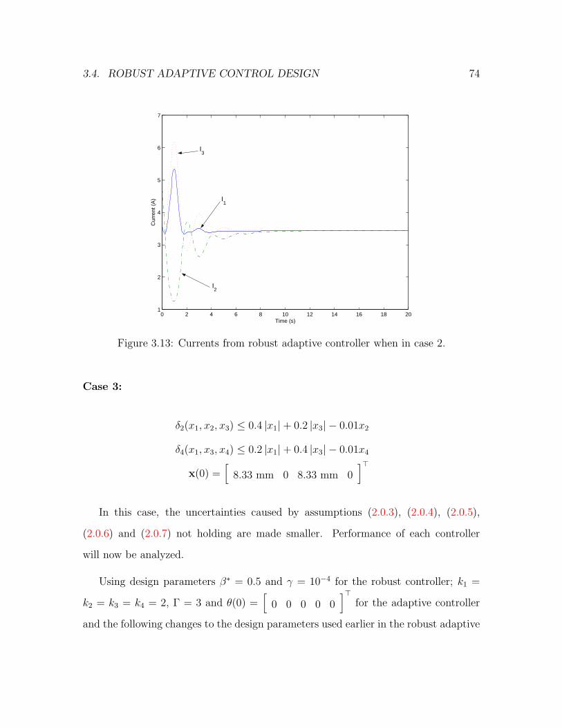
3.4. ROBUST ADAPTIVE CONTROL DESIGN 74
0 2 4 6 8 10 12 14 16 18 201
2
3
4
5
6
7
Time (s)
Cur
rent
(A
)I3
I1
I2
Figure 3.13: Currents from robust adaptive controller when in case 2.
Case 3:
δ2(x1, x2, x3) ≤ 0.4 |x1| + 0.2 |x3| − 0.01x2
δ4(x1, x3, x4) ≤ 0.2 |x1| + 0.4 |x3| − 0.01x4
x(0) =[
8.33 mm 0 8.33 mm 0
]>
In this case, the uncertainties caused by assumptions (2.0.3), (2.0.4), (2.0.5),
(2.0.6) and (2.0.7) not holding are made smaller. Performance of each controller
will now be analyzed.
Using design parameters β∗ = 0.5 and γ = 10−4 for the robust controller; k1 =
k2 = k3 = k4 = 2, Γ = 3 and θ(0) =[
0 0 0 0 0]>
for the adaptive controller
and the following changes to the design parameters used earlier in the robust adaptive

3.4. ROBUST ADAPTIVE CONTROL DESIGN 75
controller
ε2 = 10−4, ε4 = 10−4,
k1 = 1.5, k2 = 1.5, k3 = 1.5, k4 = 1.5,
γ1 = γ2 = γ3 = γ4 = 3,
ψo1 = 0, ψo
2 = 0.5.ψo3 = 0.5, ψo
4 = 0,
p2(x1) = p2(x1) = x21 + 0.02,
p3(x1, x2, x3) =
[
∂α2
∂x2tanh
(
10∂α2
∂x2
)
+ 0.1
]
(
x21 + x2
3 + 0.02)
,
we get the responses shown in Figure 3.14. The performance of each control system
is as follows
0 2 4 6 8 10 12 14 16 18 20−10
−5
0
5x 10
−3
Time (s)
x po
sitio
n (m
)
0 2 4 6 8 10 12 14 16 18 20−0.025
−0.02
−0.015
−0.01
−0.005
0
0.005
0.01
Time (s)
y po
sitio
n (m
)
linear robust adaptive
adaptive robust
robust adaptive
linear
adaptive
robust
Figure 3.14: Case 3 response of uncertain system when using linear, robust, adaptiveand robust adaptive nonlinear controllers.

3.4. ROBUST ADAPTIVE CONTROL DESIGN 76
Controller Steady-State Error (m) Max. Current (A)
Linear 2.4963 × 10⁻⁴ 1.4933
Robust 6.9753 × 10⁻⁵ 5.7069
Adaptive 3.1737 × 10⁻⁴ 6.5066
Robust Adaptive 2.6172 × 10⁻⁵ 6.1068
The disk’s final position should be at least within 0.1 mm. The linear and adaptive
controllers do not meet this performance requirement while both the robust and
robust adaptive controllers surpass it. The robust adaptive control system has a
better error but its maximum current is higher then that of the robust controller.
However, as already mentioned before, chattering of the robust controller currents
may cause practical difficulties. From a practical viewpoint, the robust adaptive
controller is the most desirable of the feedback systems as long as the actuators can
support the higher currents it tends to use.

Chapter 4
Implementation
The planar magnetic levitation device is built and shown in Figure 4.1 and Figure
4.2. Due to hardware limitations of the device, which are described in the following,
the nonlinear controllers developed in the previous chapter cannot be tested on the
system. However, some modelling and control principles of this system are experi-
mentally confirmed with two smaller testbeds.
Figure 4.1: Top view of planar magnetic levitation device.
77
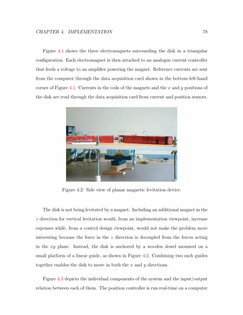
CHAPTER 4. IMPLEMENTATION 78
Figure 4.1 shows the three electromagnets surrounding the disk in a triangular
configuration. Each electromagnet is then attached to an analogue current controller
that feeds a voltage to an amplifier powering the magnet. Reference currents are sent
from the computer through the data acquisition card shown in the bottom left-hand
corner of Figure 4.1. Currents in the coils of the magnets and the x and y positions of
the disk are read through the data acquisition card from current and position sensors.
Figure 4.2: Side view of planar magnetic levitation device.
The disk is not being levitated by a magnet. Including an additional magnet in the
z direction for vertical levitation would, from an implementation viewpoint, increase
expenses while, from a control design viewpoint, would not make the problem more
interesting because the force in the z direction is decoupled from the forces acting
in the xy plane. Instead, the disk is anchored by a wooden dowel mounted on a
small platform of a linear guide, as shown in Figure 4.2. Combining two such guides
together enables the disk to move in both the x and y directions.
Figure 4.3 depicts the individual components of the system and the input/output
relation between each of them. The position controller is run real-time on a computer

CHAPTER 4. IMPLEMENTATION 79
ControllerPosition
ControllerCurrent
Amplififer Electromagnet Disk
CurrentSensor
SensorPosition
IrefVref Vm
(x, y)
Icoil
Figure 4.3: Overview of interfaces in magnetic levitation device.
using WinCon designed by Quanser Consulting. The controller calculates a current
based on the position of the disk measured by the position sensors, and the currents
running through the coils measured by the current sensor. The reference current is
an input to a current controller that computes a voltage based on the present current
in the coils of the magnet. The power amplifier outputs a high-voltage signal to the
magnet depending on the reference voltage from the current control system. Next are
the nonlinear dynamics between the magnet and the disk. The force acting on the
disk depends on the current in the magnet coils, the air gap, and various constants
such as the dimensions and permeabilities of the disk and the cores. As the disk
moves in the x and y directions along the two linear guides, the position sensors
continuously measure the position of disk. The position of the disk and the currents
in the magnets measured by the sensors are inputs to the controller in the next loop.
The individual components of the system are described in detail in Section 4.1.
Descriptions of how the components operate, reasons why a certain technology was
chosen, consideration taken and problems encountered are explained in each section.
The discussion begins with the electromagnets and steps back to the current con-
troller. The guides and position sensors are then explained, followed by the software
and interface used to implement the controller. This completes the description of the

4.1. SYSTEM COMPONENTS 80
system. In Section 4.2, different procedures considered for finding the model param-
eters are examined. The section concludes with a definitive modelling methodology
that is used later to achieve some fairly impressive control results on actual systems.
Section 4.3 describes two simpler testbeds that are primarily designed to verify ex-
perimentally the principles of the three-magnet system and isolate the problem that
is causing it to operate only partially. Individually, the setups also offer some sub-
stantial modelling and applied nonlinear motion control results as well. This section
closes with a discussion on the issues encountered in the full three-magnet system.
4.1 System Components
4.1.1 Magnet
The electromagnet cores, shown in Figure 4.1, have a cross sectional area of 5×5 cm2
and are 40 cm long. These dimensions were chosen to obtain substantial strength
from inefficient rectangular magnets (see e.g., [1]). In particular, the cross sectional
area of the cores should be considerably smaller than the length of the core. The cores
were originally 10 × 10 × 10 cm3 and the attractive magnetic force was only exerted
along the outer edge of the core’s face. In [1], the magnetic flux density inside an ideal
solenoid is compared with the magnetic flux density of two solenoids of finite length.
It is shown that the solenoid with a length to diameter ratio of 1, Ld
= 1, has half the
magnetic flux density of an ideal solenoid. On the other hand, a solenoid with Ld
= 10
is about the same strength as the ideal solenoid. This observation is consistent with
the numerical experiments done in FEMLAB for bar magnets and is briefly discussed
in Appendix A.2. Narrow magnets are needed to attain sufficient force to move the
disk but this increases fringing. Thus, to avoid the problems discussed above and
increase the strength of each electromagnet, the original magnets were each cut into

4.1. SYSTEM COMPONENTS 81
Magnet No. of Windings Resistance (Ω) Inductance (mH)1 490 5.3 40.52 482 5.0 42.43 503 5.8 50.4
Table 4.1: Measured resistance and inductance of electromagnets.
four 10 × 5 × 5 cm3 rectangles and stacked lengthwise to make a long bar magnet
with a length to diameter ratio of about
L
d=
40 cm
5 cm= 8. (4.1.1)
Magnet strength is further increased by using laminated cores made of low-copper
soft steel. Pure iron and permalloy 80 were considered first but no supplier was found
that could furnish pure iron of the dimensions needed and permalloy is too expensive.
The cores are wound with 22-Gauge magnet wire which can withstand current bursts
of 10 A and continuous currents of 6 A without the insulator coating melting. This
limit becomes a controller constraint - current must now be both positive and less
then 10 A.
The resistance and inductances measured for each magnet is shown in Table 4.1.
They are described by the following transfer functions
Icoil1 =1
0.041s+ 5.3Vm1
Icoil2 =1
0.042s+ 5.0Vm2
Icoil3 =1
0.050s+ 5.8Vm3
(4.1.2)
where for i = 1, 2, 3, Vmi is the voltage delivered by the amplifier connected to magnet
i.

4.1. SYSTEM COMPONENTS 82
4.1.2 Power Amplifier
The power amplifier is the component driving current in the electromagnet coils. The
12A8 Advance Motion Controllers Brush Type PWM Servo Amplifier is a compact
pulse-width modulator capable of outputting continuous currents of ±6 A and peak
currents of ±12 A. This output range is suitable for the currents required by the
position controller. The servo amplifier operates in open-loop mode, thus it amplifies
its input voltage by a fixed gain. Figure 4.4 shows the signal transition between the
PWM input and the magnet output. The power amplifier also features a current
monitor that measures the current in the coils of the electromagnet. This sensor is
used by the current controller and the position controller.
Vm 1Ls+R
IcoilKm
Vref
PWM Electromagnet
Figure 4.4: Input/Output relationship between PWM and electromagnet.
Grounding and sensor noise issues are avoided using the PWM wiring setup shown
in Figure 4.5. The internal signal grounds of the PWM are isolated from the power
ground terminals. The - ref terminal is connected to the shield of the signal wire
that is connected to the ground of the data acquisition card. Noise from an unused
input is prevented by attaching the - tach to the signal gnd connector. The power
wires and motor leads are twisted so the inductance formed between the wires is
cancelled in successive twists. Thus, the power ground and high-voltage terminals of
each PWM are twisted together and attached to the 0 V and 55 V terminal of the
power supply and the motor leads carrying the voltage supplied from the PWM to
the electromagnet are also twisted (not shown in diagram). Finally, the 0 V terminal
of the power supply is connected to the ground of the data acquisition card.

4.1. SYSTEM COMPONENTS 83
curr monitor out
- ref in
+ ref in
power gnd
high voltage
signal gnd
+ tach (gnd)
Data AcquisitionCard
PowerSupply
PWM- tach in
signal
return
shield
DAC gnd
0 V
55 V
Figure 4.5: Pulse-width modulator wiring.
According to the installation notes, the majority of the noise comes from the
high-voltage switching of the motor leads. As different voltages are sent though the
leads, a capacitive coupling is formed between the leads and the signal wires. This is
significantly attenuated by appropriately shielding the signal wires.
4.1.3 Current Controller
The current controller is a feedback loop that supplies a reference voltage to the am-
plifier to achieve a desired current. In this case, the desired current is given by the
position controller (see Figure 4.3) and the current control output is the PWM refer-
ence signal, Vref. The output voltage of the PI controller is amplified by the PWM to
achieve the desired current in the coils of the electromagnet. The PWM unit actually
features its own current control system. However, the amplifier current control gives
an unsuitable steady-state error because the inductances of the electromagnets are
too large and the capacitor in the current loop cannot be varied (the capacitor de-
termines the steady-state error). To overcome this problem, the current control was

4.1. SYSTEM COMPONENTS 84
designed separately and is a simple proportion-integral controller with the structure
D(s) = Kp +KI
s, (4.1.3)
where Kp, KI > 0. Figure 4.6 shows the PI compensator with the power amplifier,
the electromagnet and a sensor gain Ks.
KI
Kp
+++
−Iref 1
Ls+R
IcoilKm
Vref Vm
Ks
1s
PI Controller
PWM Electromagnet
Figure 4.6: Current controller structure.
The closed-loop system that successfully tracks a reference current is thus
Icoil =KmKs (Kps+KI)
Ls2 + (R +KmKsKp) s+KmKsKI
Iref. (4.1.4)
The proportional gain, Kp, and integral gain, KI , were tuned using the magnets
transfer functions (4.1.2) such that the best tracking could be achieved while keeping
overshoot low and ensuring the output voltage is confined within the ±15 V limit of
the + ref connector of the PWM. The current going through the coils is twice the
current monitor reading. Thus the sensor gain, Ks, from the PWM’s current monitor
is Ks = 2 A/V.
The PI current controller was implemented in both an analogue circuit and digi-
tally in WinCon. The original reason to design an analogue circuit, shown in Figure
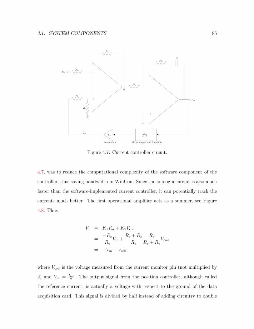
4.1. SYSTEM COMPONENTS 85
Re
Re
R1
Re
Re
Ci
V1
Rf
Ks
Sensor Gain
Icoil
−
+
+
−
Electromagnet and Amplififier
Km
Ls+R
Vref
Vin
Figure 4.7: Current controller circuit.
4.7, was to reduce the computational complexity of the software component of the
controller, thus saving bandwidth in WinCon. Since the analogue circuit is also much
faster than the software-implemented current controller, it can potentially track the
currents much better. The first operational amplifier acts as a summer, see Figure
4.8. Thus
V1 = K1Vin +K2Vcoil
=−Re
Re
Vin +Re +Re
Re
Re
Re +Re
Vcoil
= −Vin + Vcoil,
where Vcoil is the voltage measured from the current monitor pin (not multiplied by
2) and Vin = Iref2
. The output signal from the position controller, although called
the reference current, is actually a voltage with respect to the ground of the data
acquisition card. This signal is divided by half instead of adding circuitry to double

4.1. SYSTEM COMPONENTS 86
the current monitor output to get Icoil.
Re
Re
Re
Re
+
−
V1+
+V1
K1
K2
Vin
VcoilVcoil
Vin
Figure 4.8: Summer operational amplifier.
Vref
R1
CiRf
−
+
V1
V1 VrefK3(s)
Figure 4.9: Proportional-integral operational amplifier.
Figure 4.9 depicts the second operational amplifier that implements the gains of
the PI controller. The circuit analysis from the input, the reference signal Vin, to the
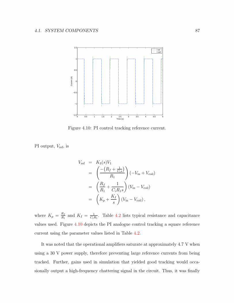
4.1. SYSTEM COMPONENTS 87
0 0.5 1 1.5 2 2.5 3 3.5 4 4.5 5−1.5
−1
−0.5
0
0.5
1
1.5
Time (s)
Cur
rent
(A
)
I refI coil
Figure 4.10: PI control tracking reference current.
PI output, Vref, is
Vref = K3(s)V1
=
(
−(
Rf + 1Cis
)
R1
)
(−Vin + Vcoil)
=
(
Rf
R1
+1
CiR1s
)
(Vin − Vcoil)
=
(
Kp +KI
s
)
(Vin − Vcoil) ,
where Kp =Rf
R1and KI = 1
CiR1. Table 4.2 lists typical resistance and capacitance
values used. Figure 4.10 depicts the PI analogue control tracking a square reference
current using the parameter values listed in Table 4.2.
It was noted that the operational amplifiers saturate at approximately 4.7 V when
using a 30 V power supply, therefore preventing large reference currents from being
tracked. Further, gains used in simulation that yielded good tracking would occa-
sionally output a high-frequency chattering signal in the circuit. Thus, it was finally

4.1. SYSTEM COMPONENTS 88
Parameter ValueRe 10kΩRf 20kΩR1 5kΩCi 50nF
Table 4.2: Typical resistance and capacitance values used for PI control.
decided to implement digitally in WinCon. This makes it convenient to test differ-
ent Kp and KI gains. In some cases, it was desired to minimize the PI voltage at
the expense of steady-state error. For instance, this is done when using controllers
with large current transients or high current biases and when testing with large step
inputs. The digital PI controller is used in all the results shown later in this chapter.
4.1.4 Disk and Linear Guides
Due to budget constraints and because of a sensing issue, discussed in the next section,
the disk is not being levitated by a fourth magnet or by an air bearing system. Instead,
linear guides are used to provide the disk with movements in the x and y directions.
A linear guide consists of a small platform that rides on one or more rails over ball
bearings for low-friction movement. Linear guides are often used in motion control
but usually in these applications the platform is actuated by a motor. In this case,
we require a guide that is unactuated since the magnets will be moving the disk. The
disk is constrained to move about a small region in the xy plane. Thus, linear guides
that are compact and that can be placed one on top of the other perpendicularly are
needed. Further, the guide must be as light as possible to minimize the current needed
to move the disk and the guide it is attached to. The Thomson Microstage linear
guide was chosen because it is constructed of a lightweight alloy, provides low-friction
precise motions and, as shown in Figure 4.11, can be mounted in an X-Y fashion.
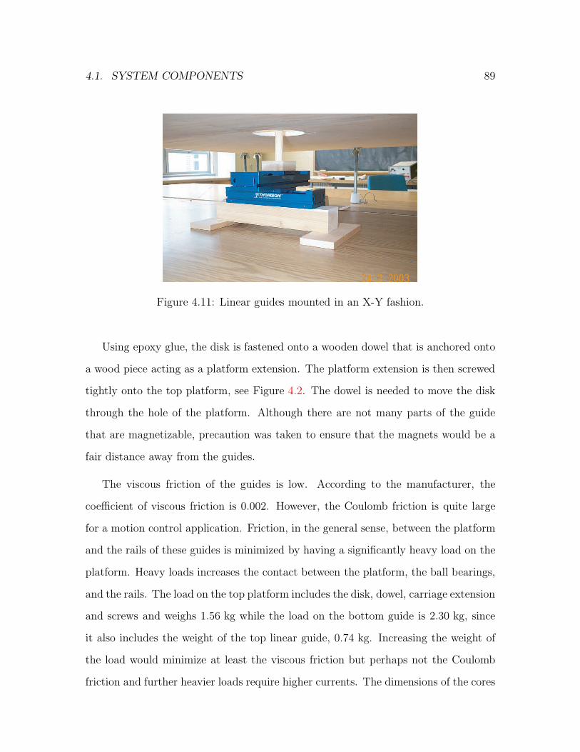
4.1. SYSTEM COMPONENTS 89
Figure 4.11: Linear guides mounted in an X-Y fashion.
Using epoxy glue, the disk is fastened onto a wooden dowel that is anchored onto
a wood piece acting as a platform extension. The platform extension is then screwed
tightly onto the top platform, see Figure 4.2. The dowel is needed to move the disk
through the hole of the platform. Although there are not many parts of the guide
that are magnetizable, precaution was taken to ensure that the magnets would be a
fair distance away from the guides.
The viscous friction of the guides is low. According to the manufacturer, the
coefficient of viscous friction is 0.002. However, the Coulomb friction is quite large
for a motion control application. Friction, in the general sense, between the platform
and the rails of these guides is minimized by having a significantly heavy load on the
platform. Heavy loads increases the contact between the platform, the ball bearings,
and the rails. The load on the top platform includes the disk, dowel, carriage extension
and screws and weighs 1.56 kg while the load on the bottom guide is 2.30 kg, since
it also includes the weight of the top linear guide, 0.74 kg. Increasing the weight of
the load would minimize at least the viscous friction but perhaps not the Coulomb
friction and further heavier loads require higher currents. The dimensions of the cores
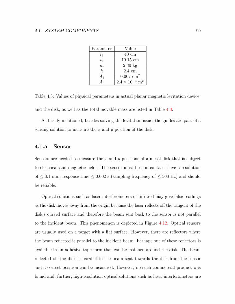
4.1. SYSTEM COMPONENTS 90
Parameter Valuel1 40 cml2 10.15 cmm 2.30 kgh 2.4 cmA1 0.0025 m2
Ar 2.4 × 10⁻³ m2
Table 4.3: Values of physical parameters in actual planar magnetic levitation device.
and the disk, as well as the total movable mass are listed in Table 4.3.
As briefly mentioned, besides solving the levitation issue, the guides are part of a
sensing solution to measure the x and y position of the disk.
4.1.5 Sensor
Sensors are needed to measure the x and y positions of a metal disk that is subject
to electrical and magnetic fields. The sensor must be non-contact, have a resolution
of ≤ 0.1 mm, response time ≤ 0.002 s (sampling frequency of ≤ 500 Hz) and should
be reliable.
Optical solutions such as laser interferometers or infrared may give false readings
as the disk moves away from the origin because the laser reflects off the tangent of the
disk’s curved surface and therefore the beam sent back to the sensor is not parallel
to the incident beam. This phenomenon is depicted in Figure 4.12. Optical sensors
are usually used on a target with a flat surface. However, there are reflectors where
the beam reflected is parallel to the incident beam. Perhaps one of these reflectors is
available in an adhesive tape form that can be fastened around the disk. The beam
reflected off the disk is parallel to the beam sent towards the disk from the sensor
and a correct position can be measured. However, no such commercial product was
found and, further, high-resolution optical solutions such as laser interferometers are
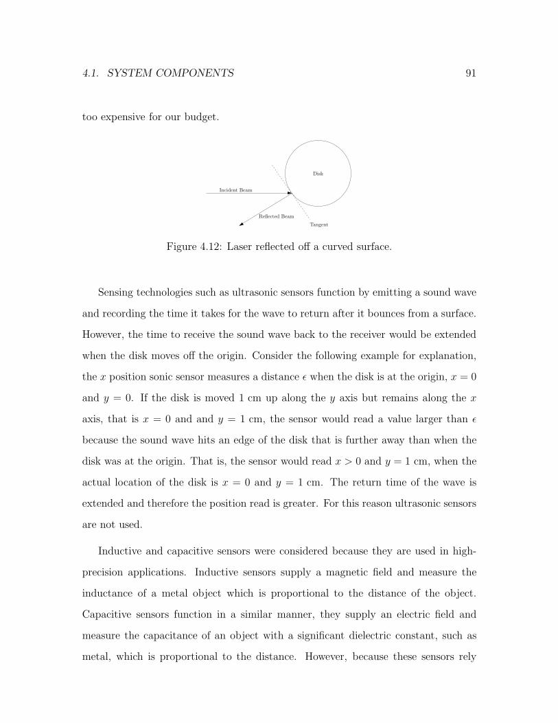
4.1. SYSTEM COMPONENTS 91
too expensive for our budget.
Incident Beam
Reflected Beam
Tangent
Disk
Figure 4.12: Laser reflected off a curved surface.
Sensing technologies such as ultrasonic sensors function by emitting a sound wave
and recording the time it takes for the wave to return after it bounces from a surface.
However, the time to receive the sound wave back to the receiver would be extended
when the disk moves off the origin. Consider the following example for explanation,
the x position sonic sensor measures a distance ε when the disk is at the origin, x = 0
and y = 0. If the disk is moved 1 cm up along the y axis but remains along the x
axis, that is x = 0 and and y = 1 cm, the sensor would read a value larger than ε
because the sound wave hits an edge of the disk that is further away than when the
disk was at the origin. That is, the sensor would read x > 0 and y = 1 cm, when the
actual location of the disk is x = 0 and y = 1 cm. The return time of the wave is
extended and therefore the position read is greater. For this reason ultrasonic sensors
are not used.
Inductive and capacitive sensors were considered because they are used in high-
precision applications. Inductive sensors supply a magnetic field and measure the
inductance of a metal object which is proportional to the distance of the object.
Capacitive sensors function in a similar manner, they supply an electric field and
measure the capacitance of an object with a significant dielectric constant, such as
metal, which is proportional to the distance. However, because these sensors rely
4.1. SYSTEM COMPONENTS 92
on magnetic or electric fields to get their measurements, the electromagnetic field
generated by the magnets moving the disk may interfere with those of the sensors
and cause false readings. As a result, they were discarded as a reliable source of
reading position.
Another option was tracking the position of the disk by mounting a CCD camera
looking down on the xy plane of the experiment. This sensing technology was used
in a magnetic suspension system in [5] with a resolution of 0.43 mm. The camera
alternative requires substantial effort in designing the signal processing to get the
positions. Further, its response time is too slow and the resolution is inadequate,
> 0.1 mm.
Fast high-resolution measurements of the disk’s (x, y) position can be obtained by
mounting optical encoders on the platform of each linear guide and attaching their
shafts with a fishing line that is fastened at each end of the guides. Figure 4.13 shows
how the encoder is anchored on the linear guide. As the disk moves about the xy
plane, the platform on each guide moves and the shafts on the encoders rotate. The
fishing line is fastened tightly to prevent slippage of the line. As the shaft rotates,
the encoder outputs a count that is translated in a linear distance using the sector
formula
x = r∆θn
=0.125 in
2× 1 m
39.37 m× 2π rad
4 · 1024 counts× n
= 4.8704 × 10⁻⁶n m (4.1.5)
where r is the radius of the optical encoder’s shaft, ∆θ is the change in angle of
the shaft and n is the number of counts the encoder is reading. The resolution is
four times the counts per revolution of the sensors because the data acquisition card

4.1. SYSTEM COMPONENTS 93
decodes in quadrature mode. Thus assuming ideal operation, the sensor achieves
about 5µm resolution instead of 20µm.
Figure 4.13: Linear guide and sensor setup.
Tests were made on each encoder by moving the linear guide platform at different
points and comparing the output of the encoder with a manual reading off a ruler
fastened on the side of the guide. It was found that there was a consistent error
of 0.5 mm for every 1 cm of distance. For instance, when the platform was moved
to 4 cm the encoder measured 3.80 cm and when moved to 1 cm it read 0.95 cm.
However, when the platform was moved at a certain distance and moved back to its
original position the encoder would correctly measure a distance of 0 at the platform’s
final position. For example, if the platform was moved 5 cm and moved back the same
distance, the encoder would measure 0 cm. Thus it appears from the second tests that
there is no slippage of the fishing line on the shaft. However, the 5% error in the first
test could not be rooted to any other problem. Since the error is consistent and the
resolution is still at least 0.1 mm, a 1.05 adjustment was made in the transformation
that calculates linear position from the optical encoder’s count.
Transducers in place of the optical encoders could also be used but concerns were
made on the amount of friction they would introduce.

4.1. SYSTEM COMPONENTS 94
4.1.6 Real-time Controller Software and Interface
All the nonlinear controllers designed are implemented in the Simulink environment
and are run using the Wincon software platform by Quanser Consulting. WinCon
is a realtime software that extends Simulink and offers a variety of Simulink blocks
to interact with the Quanser MultiQ PCI data acquisition card. Such blocks that
communicate externally are A/D input, encoder input and D/A output. WinCon
generates the code from a Simulink model and the code is run on the computer. The
controller can be started locally on the machine the code was built from or, since this
is a client-server program, can be run from a remote machine via the Internet. The
controller can be run at a sampling rate of at least 1 kHz and control parameters
can be adjusted in real-time, that is, the changes are applied immediately while the
controller is running.
Nss+N
x
x
y
y
Input
Encoderto Pos.Count
Input
Analogue2 A/V
Output
Analogue
Icoil 1
Icoil 2
Icoil 3
Iref 1
Iref 2
Iref 3
Nss+N
Position
Controller
Figure 4.14: Interface between position controller and magnetic levitation device.
Figure 4.14 shows the various interfaces between the position controller and sen-
sors. The three reference currents computed by the position controller are sent to the
analogue output box. These signals are outputted from the the D/A outputs on the
DAC’s terminal board, shown in Figure 4.1. The actual currents going through the
electromagnets coils are taken from the current monitor pins on the power amplifiers.
In the software, current measured in the coils of the electromagnets is received from

4.1. SYSTEM COMPONENTS 95
the analogue input block. The x and y positions of the disk are measured from the
optical encoders using the encoder inputs. The encoder input gives the count and
then the sector formula described in (4.1.5) calculates the positions from the count.
The disk velocity is attained using a high-gain observer on the x and y displacements,
as shown in Figure 4.14.

4.2. FINDING MODEL PARAMETERS 96
4.2 Finding Model Parameters
Consider again the system model (2.3.2), included here for convenience
x1 = x2
x2 = − 1
2mµoA1
[
ϕ1(x1, x3)(x1 + d)I21 + ϕ2(x1, x3)
(
x1 −d
2
)
I22
+ ϕ3(x1, x3)
(
x1 −d
2
)
I23
]
x3 = x4
x4 = − 1
2mµoA1
[
ϕ1(x1, x3)(−x3)I21 + ϕ2(x1, x3)
(
x3 +
√3
2d
)
I22
+ ϕ3(x1, x3)
(
x3 −√
3
2d
)
I23
]
(4.2.1)
where
ϕ1(x1, x3) =N2
1(
L1
µ1A1+ L2
µ2A2+
√(x1+d)2+x2
3
µ0A1
)2√
(x1 + d)2 + x23
ϕ2(x1, x3) =N2
2
L1
µ1A1+ L2
µ2A2+
s
(
x1− d2
)2
+
(
x3+√
3
2d
)2
µ0A1
2√
(
x1 − d2
)2
+(
x3 +√
32d)2
ϕ3(x1, x3) =N2
3
L1
µ1A1+ L2
µ2A2+
s
(
x1− d2
)2
+
(
x3−√
3
2d
)2
µ0A1
2√
(
x1 − d2
)2
+(
x3 −√
32d)2
,
and notice that the only unknown parameters in (4.2.1) is the permeability of the
cores, µ1, and of the disk, µ2. These permeabilities are found by measuring the
inductance of the electromagnet for a given position of the disk. Then, using an

4.2. FINDING MODEL PARAMETERS 97
inductance expression describing the inductance of the electromagnet with respect
to the air gap between the core and the disk, the permeabilities can be found. The
inductance expression is developed by using the flux linkage formula
λ = NΦ, (4.2.2)
where N is the number of windings and Φ is the magnetic flux, and the relationship
between inductance and flux linkage
λ = L(z)I. (4.2.3)
Combining equations (4.2.2) and (4.2.3) with the one-dimensional flux relationship
described in (2.1.7),
Φ =NI
l1µ1A1
+ l2µ2A1
+ zµoA1
, (4.2.4)
where l1 is the core’s length, l2 is the disk diameter, µ1 = µr1µ0, µ2 = µr2µ0 and
µ0 = 4π× 10−7 H/m is the permeability of free space, gives the relationship between
inductance, L, and the air gap z,
L(z) =1
l1µ1A1N2 + l2
µ2A1N2 + zµoA1N2
. (4.2.5)
Assuming the permeability of the core, µ1, and of the disk, µ2, are equal and measuring
the zero air gap inductance, L(0), the relative permeability µr1 = µr2 can be found.
Note that assumption µ1 = µ2 is realistic because the disk is constructed of the same
material as the cores. Using the resistance and inductance measurements in Table 4.1
and the various properties in Table 4.3, the relative permeability of electromagnet 1

4.2. FINDING MODEL PARAMETERS 98
is
µ1 = µ2 =L10
N21
(
l1
A1
+l2
A2
)
µr1 = µr2 =L10
µ0N21
(
l1
A1+
l2
A2
)
=40.2 × 10⁻³ H
(4π × 10−7 H/m)(490)2
(
0.4 m
(0.05m)2+
0.10 m
(0.10 m)(2.4 × 10⁻² m)
)
= 26.9.
Similarly, the relative permeabilities of magnets 2 and 3 are
µr2 = 29.4, µr3 = 31.9.
The model parameters of the three-magnet dynamics in (4.2.1) are completely known.
However, instead of measuring the inductance and finding the relative permeabilities,
the dynamics in (4.2.1) can be expressed directly in terms of the measured inductance.
This is discussed in the next section.
4.2.1 Inductance Models
Expressing the model in terms of inductance yields a model that is more intuitive
in a practical sense and results in dynamics that are presented in a more compact
form by grouping various parameters together. In the first part of this section, the
force between an electromagnet and a disk in the one-dimensional case is developed
using the new presentation of the inductance relationship in (4.2.5). The resulting
dynamics are expressed in terms of inductance and are entirely equivalent to the one-
dimensional result obtained earlier in Section 2.1. Due to the modelling uncertainty
concerns outlined in Chapter 2, an alternative expression of inductance is discussed
in the second part of this section that is developed experimentally. This, on the

4.2. FINDING MODEL PARAMETERS 99
other hand, is not equivalent to force expression in Section 2.1. The reasons why
another expression for inductance is considered along with the problems associated
with deriving it are discussed.
Model A
The magnetic force between a single electromagnet and a disk in the one-dimensional
case is now found using inductance as opposed to the analysis done in Section 2.1.
Change inductance relationship (4.2.5) into
L(z) =1
l1µ1A1N2 + l2
µ2A1N2 + zµoA1N2
=N2
(
l1µ1A1
+ l2µ2A1
)
(
1 + z
µoA1
“
l1µ1A1
+l2
µ2A1
”
)
=L0
1 + za
(4.2.6)
where
L0 =N2
l1µ1A1
+ l2µ2A1
a = µ0A1
(
l1
µ1A1+
l2
µ2A1
)
=µ0A1N
2
L0.
(4.2.7)
The inductance of the electromagnet when the disk is attached to the face of the core
is L0 = L(0), and the decay parameter, a, is based on the reluctance principle in [1].
Inductance expressed in this manner is called model A.
Alternatively to the relationship in (2.1.8), magnetic energy can be expressed in
terms of inductance as
E(z, I) =1
2L(z)I2, (4.2.8)
where z is the air gap distance between the magnet and the disk, L(z) is the mutual
inductance of the electromagnet and the disk as a function of the air gap, and I is
4.2. FINDING MODEL PARAMETERS 100
the current in the coils of the electromagnet. By taking the derivative with respect
to the air gap we obtain the force exerted by the electromagnet on the disk
F (z, I) =∂E(z, I)
∂z. (4.2.9)
Using relationships (4.2.8) and (4.2.9), the magnetic force between an electromagnet
and a disk is
F (z, I) =∂
∂z
(
1
2L(z)I2
)
=1
2I2∂L(z)
∂z
= −L0
2a
1(
1 + za
)2 I2
=−b
(
1 + za
)2 I2,
(4.2.10)
where b = L0
2a. We stress that the force expression in (4.2.10) is equivalent to that
in (2.1.10). The three-magnet dynamics (4.2.1) can be developed following the same
procedure illustrated in Section 2.2 and Section 2.3.
Model B
An alternative way of expressing inductance in terms of air gap, herein called model
B, is described in [13] for a 1 DOF magnetic levitation apparatus. Model B has a
similar hyperbolic expression as in (4.2.6) but one difference is that parameter a is
found experimentally rather than being calculated using the relationship in (4.2.7).
This model can therefore be entirely derived using experimental results.
The motivation for a purely experimental model is due to some concern on the
accuracy of the model developed in Chapter 2 (see Section 2.4). Namely the main
assumptions when modelling such an electromechanical system are that the air gaps
be small and the permeability of the cores be much larger then the permeability of air.

4.2. FINDING MODEL PARAMETERS 101
Under these conditions it is fair to assume that fringing can be neglected. Fringing
is illustrated in Appendix A.1. These assumptions are used in [1] and even in many
of the problems illustrated in [13], except when an actual magnetic levitation device
is being considered and the dynamics are instead found experimentally to take into
account fringing and other uncertainties. Various examples in [13] assume that the
air gap, z, is much smaller then the width of the core, w, and the height of the core,
h, thus z w and z h, and further consider the permeability of the cores to be
infinite, µ = ∞.
In our case, the core used has a width and height of 5 cm and the disk is usually
at least z > 1 cm, so at best the air gap is only smaller then the magnet width or
height, z < w or z < h, and not much smaller. The cores have a relative permeability
between 27 and 32, thus µ is far from being infinite. The material of our cores have a
low relative permeability compared to other materials often used in electromagnets.
Pure iron has a relative permeability of at least 700 and iron-steel has at least about
200. In conclusion, both major modelling assumptions do not hold. Physically, low
permeability and large air gaps promote excess fringing.
Another concern is the effect of mutual inductance. Mutual inductance between
electromagnets is present when the changing flux of one magnet induces a voltage
in the coils of another magnet. This cross-coupling behaviour could potentially be a
source of major uncertainty in the dynamics.
The inductance of the disk as it moves from the face of the electromagnet, z = 0,
to z = ∞, can be described by the following hyperbolic function
L(z) = L1 +L0
1 + za
, (4.2.11)
where L0 + L1 is the inductance of the magnet when the disk is at z = 0, L1 is the

4.2. FINDING MODEL PARAMETERS 102
electromagnet inductance when the disk is at z = ∞, or in practical terms is distant,
and a > 0 is the factor that affects the rate at which the inductance decreases as
the disk moves away from the magnet. By determining the parameters L0, L1, and
a experimentally, one obtains a model of the system that can be compared to model
A which is based on theoretical principles. To experimentally find L0, L1, and a,
we measure the inductance for different positions of the disk and fit the function in
(4.2.11) to the resulting data points.
In model A the inductance of the core decreases to 0 as the disk moves away,
that is L(∞) = 0, while in model B (and in practice) this is not the case. This is
the first difference between the models. The second difference is that in model A
the inductance of the magnet is measured once when the air gap is zero, L(0) = L0
and the decay function a is calculated using the expression in (4.2.7) rather than,
as in model B, being found on the basis of a best-fit curve mapped to a series of
experimental data points. So while model B is entirely experimental, model A is not.
4.2.2 Measuring Inductance
In model A, the inductance at z = 0 must be measured and in model B the inductance
must be measured for different disk locations. Inductance of the electromagnet for a
given air gap can be measured using two techniques: using reference step signals and
doing analysis in the time-domain, method 1, or using a sinusoidal reference and
doing analysis in the frequency-domain, method 2. Both measurements methods
are described followed by a discussion of the preferred method in Section 4.2.3.
Method 1
In method 1, a step input is given to the electromagnet and the response is saved on
a computer using WinCon and the DAC that reads the currents in the coils. Thus,

4.2. FINDING MODEL PARAMETERS 103
for a given disk location, a step input is given and the response is observed. The
response of the magnet to a step of amplitude A in the time-domain is
y(t) =KmA
R
(
1 − e
(
−RL
(t−to))
)
= c1(
1 − ec2(t−to))
, t ≥ to,
(4.2.12)
where Km is PWM’s amplification, R is the coil resistance, to is the time the reference
is given, L is the inductance, c1 = KmAR
and c2 = −RL. Using a curve fitting optimiza-
tion algorithm we find c1 = KmAR
and c2 = −RL
that best fit the experimental data.
Since Km, A, and R are known, the inductance L can be found. The inductance is
measured four times with step inputs V = 1 . . . 6 V. The mean of the four samples
is the inductance of the electromagnet for a certain current step amplitude when the
disk is at a certain position. Prior to taking the average, the variance of the four
samples is analyzed to omit any inaccurate results from being taken into account.
Method 2
In method 2, the voltage and current in the electromagnet are measured using a
multimeter when using a 60 Hz sinusoidal signal as the input. In the frequency-
domain, the electromagnet frequency response is
I(jω) =1
jωL+RV (jω), (4.2.13)
where I is the current response, V in the input voltage, ω is the frequency of the
input signal, L is the inductance, and R is the coil resistance. The current, voltage,
and resistance are measured and the angular frequency is ω = (2π rad/Hz)(60Hz) =
120π rad. For a certain disk location, the inductance of the electromagnet is then
4.2. FINDING MODEL PARAMETERS 104
found by taking the gain of (4.2.13) and solving for L
L =1
ω
√
( |V (ω)||I(ω)|
)2
− R2. (4.2.14)
4.2.3 Modelling Procedure
Four possible procedures are available to find the model parameters - measuring the
inductance using method 1 or 2 to build model A or model B. In this Section, it is
shown that model B cannot be practically developed because of the low permeability
of the cores and the disk. The model parameters can however be described accu-
rately by model A using either inductance measuring method. Even though both
methods yield accurate model A parameters, method 2 is chosen over method 1 and
the reasons are discussed. The results shown in this section were performed on the
magnets when they were positioned in the two-magnet setup shown in Figure 4.18. In
this configuration, the electromagnets are placed on opposite sides of the disk along
a straight line. This two-magnet testbed is a control experiment designed to test
modelling accuracy, discussed later in Section 4.3.1.
Model B Issues
Finding the parameters of model B, L0, L1, a, using method 1 and 2 will now be
discussed. For model B, the inductance of the electromagnets is measured at different
disk positions with respect to each core - beginning at zi = 0 and going towards zi = 2d
for magnet i = 1, 2. This model is entirely derived from a series of experimental runs.
For magnet 1, Figure 4.15 depicts the results using method 1 and Figure 4.16 shows
the results using method 2. Similar results were found using other magnets in the
two-magnet setup and when the magnets were used in the three-magnet configuration.

4.2. FINDING MODEL PARAMETERS 105
0 1 2 3 4 5 6 7 889.4
89.6
89.8
90
90.2
90.4
90.6
90.8
91
91.2
91.4Magnet 1
z (cm)
indu
ctan
ce (
mH
)
Figure 4.15: Model B inductance samples using method 1.
0 1 2 3 4 5 6 7 835.2
35.3
35.4
35.5
35.6
35.7
35.8
35.9
36Magnet 1
z (cm)
indu
ctan
ce (
mH
)
Figure 4.16: Model B inductance samples using method 2.
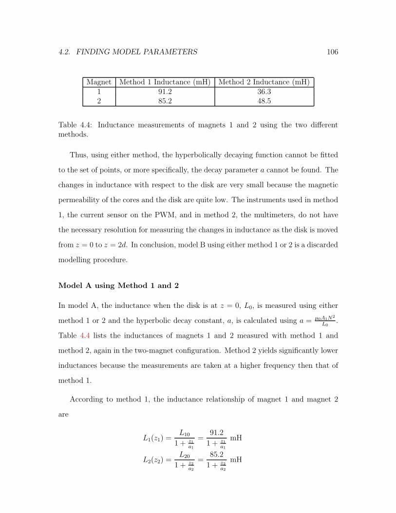
4.2. FINDING MODEL PARAMETERS 106
Magnet Method 1 Inductance (mH) Method 2 Inductance (mH)1 91.2 36.32 85.2 48.5
Table 4.4: Inductance measurements of magnets 1 and 2 using the two differentmethods.
Thus, using either method, the hyperbolically decaying function cannot be fitted
to the set of points, or more specifically, the decay parameter a cannot be found. The
changes in inductance with respect to the disk are very small because the magnetic
permeability of the cores and the disk are quite low. The instruments used in method
1, the current sensor on the PWM, and in method 2, the multimeters, do not have
the necessary resolution for measuring the changes in inductance as the disk is moved
from z = 0 to z = 2d. In conclusion, model B using either method 1 or 2 is a discarded
modelling procedure.
Model A using Method 1 and 2
In model A, the inductance when the disk is at z = 0, L0, is measured using either
method 1 or 2 and the hyperbolic decay constant, a, is calculated using a = µ0A1N2
L0.
Table 4.4 lists the inductances of magnets 1 and 2 measured with method 1 and
method 2, again in the two-magnet configuration. Method 2 yields significantly lower
inductances because the measurements are taken at a higher frequency then that of
method 1.
According to method 1, the inductance relationship of magnet 1 and magnet 2
are
L1(z1) =L10
1 + z1
a1
=91.2
1 + z1
a1
mH
L2(z2) =L20
1 + z2
a2
=85.2
1 + z2
a2
mH

4.2. FINDING MODEL PARAMETERS 107
where z1 is the air gap with respect to magnet 1, z2 is the air gap with respect to
magnet 2, L10 = L1(0) is the zero air gap inductance of magnet 1, L20 = L2(0) is the
zero air gap inductance of magnet 2, and the decay factors a1 and a2 are
a1 =µ0A1N
21
L10=
(4π × 10−7)(0.05 m)2(419)2
91.2 × 10−3= 6.05 × 10⁻³ m−1
a2 =µ0A1N
22
L20=
(4π × 10−7)(0.05 m)2(482)2
85.2 × 10−3= 8.57 × 10⁻³ m−1.
Alternatively, using method 2 the expressions become
L1 =36.3
1 + z1
a2
mH
L2 =48.5
1 + z2
a2
mH,
where
a1 =µ0A1N
21
L10=
(4π × 10−7)(0.05 m)2(419)2
36.3 × 10−3= 1.52 × 10⁻² m−1
a2 =µ0A1N
22
L20=
(4π × 10−7)(0.05 m)2(482)2
48.5 × 10−3= 1.50 × 10⁻² m−1.
Figure 4.17 compares the inductance expressions from method 1 and 2 for each mag-
net.
The model parameters developed using model A with either method 1 or 2 were
used in a controller designed for the two-magnet system and the disk was successfully
stabilized to the origin. This seems to indicate that model A accurately represents the
magnetic force of each electromagnet, at least when the disk travels within a certain
range. More specifically, using the hyperbolic decay based on the air gap reluctance
principle, a = µ0A1N2
L0, offers satisfactory control performance in two-magnet configu-
ration. Even though each method measures different values of inductance, the reason
why both methods yields successful control results is perhaps that the inductances of
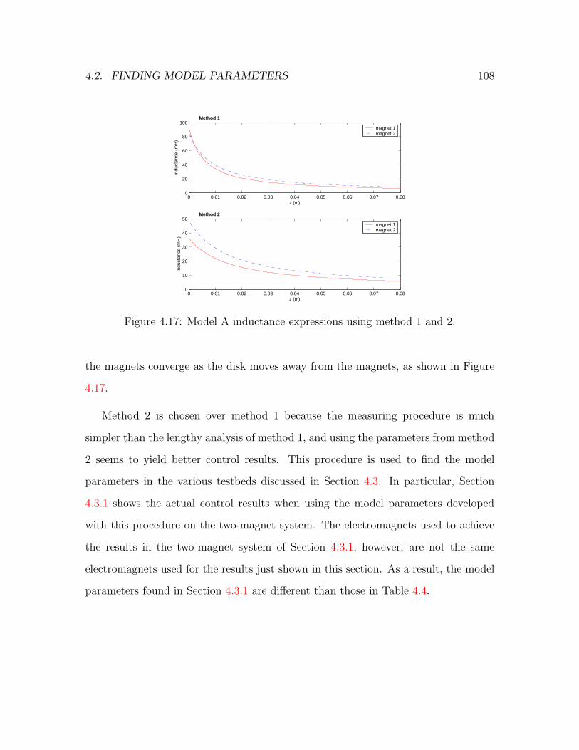
4.2. FINDING MODEL PARAMETERS 108
0 0.01 0.02 0.03 0.04 0.05 0.06 0.07 0.080
20
40
60
80
100Method 1
z (m)
indu
ctan
ce (
mH
)
magnet 1magnet 2
0 0.01 0.02 0.03 0.04 0.05 0.06 0.07 0.080
10
20
30
40
50Method 2
z (m)
indu
ctan
ce (
mH
)
magnet 1magnet 2
Figure 4.17: Model A inductance expressions using method 1 and 2.
the magnets converge as the disk moves away from the magnets, as shown in Figure
4.17.
Method 2 is chosen over method 1 because the measuring procedure is much
simpler than the lengthy analysis of method 1, and using the parameters from method
2 seems to yield better control results. This procedure is used to find the model
parameters in the various testbeds discussed in Section 4.3. In particular, Section
4.3.1 shows the actual control results when using the model parameters developed
with this procedure on the two-magnet system. The electromagnets used to achieve
the results in the two-magnet system of Section 4.3.1, however, are not the same
electromagnets used for the results just shown in this section. As a result, the model
parameters found in Section 4.3.1 are different than those in Table 4.4.

4.3. ANALYSIS 109
4.3 Analysis
The controllers designed for the planar magnetic levitation system could not be tested
due to hardware limitations that are discussed later. The exact problem in the 2 DOF
case was isolated using two smaller experiments. While these experiments were used
to troubleshoot the difficulties present in the planar magnetic levitation configuration,
the results obtained are significant and deserve close attention.
In Section 4.3.1, a two-magnet system that moves the disk along the x axis is
considered. The dynamics of this one-dimensional device are derived and the design
of a nonlinear control is summarized. Using the model parameters developed with
the modelling procedure discussed in Section 4.2, it is shown that the disk can be
stabilized with good performance. Thus, the nonlinear control result validates the
modelling procedure for this particular setup. Further, the control results using the
nonlinear controller are compared to that of a linear controller when using identical
model parameters.
The control results in Section 4.3.1 show that accurate model parameters can be
found for a one-dimensional system when the disk is aligned with the axes of the
magnets. In Section 4.3.2, a three-magnet testbed is used to show that the disk can
also be stabilized using a controller when the disk goes off the axes of the magnets.
The experiment is designed to test the two-dimensional model and, in particular, the
notion of air gaps when the disk is not aligned with a magnet. The disk however,
is still constrained to move only in the x direction so this is simpler than the full
three-magnet setup. The dynamics of this three-magnet system are given followed by
a nonlinear control design that enables the controller developed for the two-magnet
system to be used in the three-magnet system. The section ends with some results.
Lastly, Section 4.3.3 deals with the full three-magnet system using the controller

4.3. ANALYSIS 110
developed in Section 3.1. The dynamics of this system using the modelling procedure
in Section 4.2 and the 2 DOF ideal nonlinear controller are summarized. Then, the
problem encountered in the planar magnetic levitation device is discussed along with
results illustrating its behaviour.
4.3.1 Two-Magnet System
Figure 4.18: Two-magnet system experimental setup.
The experimental setup of the two-magnet system is shown in Figure 4.18. This
experimental testbed eliminates the asymmetry of the x and y guides and allows the
focus to be on the modelling of the magnetic forces. Thus the main motivation of
the two magnet system is to eliminate the y guide that had noticeably more friction
and focus on the one-dimensional problem of validating that the procedure discussed
in Section 4.2.3 obtains accurate model parameters. The dynamics of the system as
well as a nonlinear controller are given. Results comparing a linear controller and the
nonlinear controller designed using the model parameters conclude this section.

4.3. ANALYSIS 111
Dynamics
I2I1
O
MAGNET 1 MAGNET 2
Disk
d d
x
Figure 4.19: Two-magnet system diagram.
Figure 4.19 depicts the setup of the two-magnet 1 DOF system. The dynamics of
the system can be represented as
x1 = x2
x2 =−1
m
b1I21
(
1 + x1+da1
)2 − b2I22
(
1 + d−x1
a2
)2
,
(4.3.1)
where m is the mass of the system and d = 2.48 cm is the air gap between the magnets
and the disk when the disk is at the origin. Magnets 3 and 2 in Table 4.1 are magnets
1 and 2, respectively, in Figure 4.19 and the inductances of electromagnets 3 and 2
when the disk is at z1 = 0 and z2 = 0, respectively, are
L10 = 50.4 mH, L20 = 42.4 mH,
4.3. ANALYSIS 112
giving the model parameters
a1 =µ0A1N
23
L10=
(4π × 10−7)(0.05 m)2(503)2
50.4 × 10−3= 1.58 × 10⁻² m−1
a2 =µ0A1N
22
L20=
(4π × 10−7)(0.05 m)2(482)2
42.4 × 10−3= 1.72 × 10⁻² m−1
b1 =L10
2a1
= 1.59 H/m
b2 =L20
2a2
= 1.23 H/m.
(4.3.2)
This completes the model of the two-magnet system.
Controller
Recall that the three-magnet ideal nonlinear controller constructed in Section 3.1 is
based on the nonlinear controller developed in [10], Section 12.3. In fact, [10] considers
precisely the setup in Figure 4.19. This nonlinear controller is summarized as
I1 =
√
√
√
√
m(
1 + x1+da1
)2
b1ηa
I2 =
√
√
√
√
m(
1 + d−x1
a2
)2
b2ηb
(4.3.3)
where
ηa =−u+
√u2 + ε
2+ b
ηb =u+
√u2 + ε
2+ b,
b ≥ 0 is the bias current and u is a control variable to be defined later. Using the
control I1, I2 in the two-magnet system (4.3.1) yields the linear dynamics
x1 = x2
x2 = u.
4.3. ANALYSIS 113
The origin of the uncertainty-free system is stabilized by closing the feedback loop
using LQR with the weighing matrices
Q =
100 0
0 100
, R = 0.35,
that generates the gain matrix
K =[
16.9031 17.8751
]
. (4.3.4)
Results
Similarly to the simulations in the three-magnet system, the ideal nonlinear stabi-
lizer for the two-magnet system is compared with a linear controller. The system is
linearized about the origin and we obtain a gain
[I21 , I
22 ]> = KLx =
−336.5913 −165.8485
322.4925 158.9016
,
using LQR with the weighing matrices
Q =
500 0
0 500
, R =
1 0
0 1
. (4.3.5)
Figure 4.20 depicts the closed-loop response of the linear controller when the disk
is initialized at −0.51 cm. The steady-state position error in this particular case is
−0.12 cm. The currents from the linear controller in this response are shown in Figure
4.21 and the maximum current is 6.46 A. Another result when the linear controller
is used in the two-magnet system is shown in Figure 4.22. In this case, the disk
starts at 1.05 cm and ends up at 0.52 cm with a maximum peak current of 9.17 A
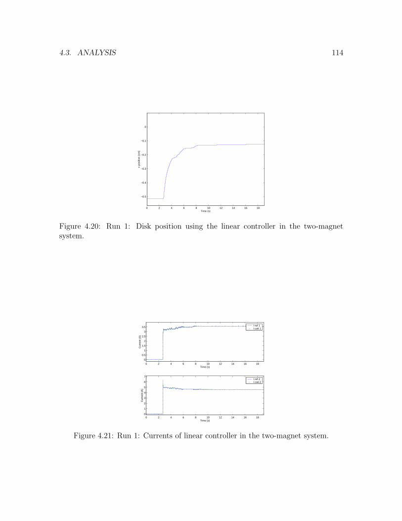
4.3. ANALYSIS 114
0 2 4 6 8 10 12 14 16 18
−0.5
−0.4
−0.3
−0.2
−0.1
0
Time (s)
x po
sitio
n (c
m)
Figure 4.20: Run 1: Disk position using the linear controller in the two-magnetsystem.
0 2 4 6 8 10 12 14 16 18
0
0.5
1
1.5
2
2.5
3
3.5
Time (s)
Cur
rent
(A
)
I ref 1I coil 1
0 2 4 6 8 10 12 14 16 180
1
2
3
4
5
6
7
Time (s)
Cur
rent
(A
)
I ref 2I coil 2
Figure 4.21: Run 1: Currents of linear controller in the two-magnet system.

4.3. ANALYSIS 115
(the currents are not shown). The steady-state error of the linear controller may be
improved using an integrator anti-windup. This shall be subject to future research.
0 2 4 6 8 10 12 14 16 18
0
0.2
0.4
0.6
0.8
1
Time (s)
x po
sitio
n (c
m)
Figure 4.22: Run 2: Disk position using the linear controller in the two-magnetsystem.
The ideal controller is now tested with the model parameters given in (4.3.2) and
the controller design parameters b = 0, ε = 1× 10⁻⁵ and the LQR gain stated earlier
in (4.3.4). Figure 4.23 is the position trajectory under the ideal controller and Figure
4.24 are the currents. The nonlinear control manages to stabilize the disk to −0.02 cm
when the disk begins at −0.81 cm with a maximum current of 8.70 A. In the another
run when the disk’s initial position is 1.99 cm, the ideal controller moves to disk at
0.06 cm from the origin with a peak current of 9.89 A. The currents are appropriately
tracked by the current controller ever though there is considerable chattering.
The ideal controller outperforms the linear controller in terms of steady-state error
even when the initial state is further away from the origin. Further, this experiment
shows that the procedure used to develop the model parameters is sufficient to sta-
bilize the disk with at least 1 mm precision. Many modelling assumptions discussed
earlier and in Chapter 2 (see Section 2.4) are now verified to be negligible with respect
to stabilizing the disk using the nonlinear controller. For instance, it has now been
shown that it is reasonable to ignore fringing and mutual inductance.

4.3. ANALYSIS 116
0 5 10 15
−0.8
−0.7
−0.6
−0.5
−0.4
−0.3
−0.2
−0.1
0
Time (s)
x po
sitio
n (c
m)
Figure 4.23: Run 3: Disk position using the ideal controller in the two-magnet system.
0 5 10 150
1
2
3
4
5
Time (s)
Cur
rent
(A
)
I ref 1I coil 1
0 5 10 150
2
4
6
8
10
12
Time (s)
Cur
rent
(A
)
I ref 2I coil 2
Figure 4.24: Run 3: Currents of ideal controller in the two-magnet system.
0 5 10 15 20 25
0
0.2
0.4
0.6
0.8
1
1.2
1.4
1.6
1.8
2
Time (s)
x po
sitio
n (c
m)
Figure 4.25: Run 4: Disk position using the ideal controller in the two-magnet system.

4.3. ANALYSIS 117
4.3.2 Three-Magnet System using Equivalent Ideal Controller
The previous experiment confirmed that the modelling procedure finalized in Section
4.2.3 is sufficiently accurate, at least when the disk travels along the magnets axes.
However, the two-magnet system is a one-dimensional setup and therefore we cannot
test the effects on the model when the disk does not travel along the axes of the
magnets. That is, the notion of air gaps in the 2 DOF case, described in the equations
(2.2.3), may not hold in the actual system. There is some concern that fringing
between magnets 2 and 3 (see Figure 1.3) would create some difficulties and also that
the disk may have been attracted to the corners of the magnets where the flux is
stronger, rather then being attracted towards their centers. Some of these concerns
were expressed in the modelling uncertainties outlined in Chapter 2 (see Section 2.4).
In this section we develop a control that enables the 1 DOF control system in
Section 4.3.1 to be used in the three-magnet system. Using the vector air gap ex-
pressions (2.2.3) in the two-dimensional case, we find a current that is used in both
magnets 2 and 3 so that they act as a single magnet. That is, by supplying this
current to magnets 2 and 3 they together supply a force that is equivalent to having
a single magnet aligned with magnet 1, as in the two-magnet system. If the control
is successful, then the force from an electromagnet on the disk when it is off the axes
of the magnet is represented correctly by our model.
The first part describes the dynamics of the three-magnet system along with some
simplifications since the disk is constrained in the x direction. In the second part, the
equivalent current control is developed, and the last part shows the results obtained
using this controller on the actual testbed.
4.3. ANALYSIS 118
Dynamics
The dynamics of the three-magnet system in terms of inductance is
x1 = x2
x2 = − 1
m
[
ϕ1(x1, x3)(x1 + d)I21 + ϕ2(x1, x3)
(
x1 −d
2
)
I22 + ϕ3(x1, x3)
(
x1 −d
2
)
I23
]
x3 = x4
x4 = − 1
m
[
ϕ1(x1, x3)(−x3)I21 + ϕ2(x1, x3)
(
x3 +
√3
2d
)
I22 + ϕ3(x1, x3)
(
x3 −√
3
2d
)
I23
]
(4.3.6)
where
ϕ1(x1, x3) =b1
(
1 +
√(x1+d)2+x2
3
a1
)2
1√
(x1 + d)2 + x23
ϕ2(x1, x3) =b2
1 +
s
(
x1− d2
)2
+
(
x3+√
3
2d
)2
a2
2
1√
(
x1 − d2
)2
+(
x3 +√
32d)2
ϕ3(x1, x3) =b3
1 +
s
(
x1− d2
)2
+
(
x3−√
3
2d
)2
a3
2
1√
(
x1 − d2
)2
+(
x3 −√
32d)2.
Note that under the modelling procedure of model B using method 2 detailed in
Section 4.2, the only difference between the dynamics of the three-magnet system
(4.2.1) developed in Chapter 2 are the expressions ϕ1, ϕ2 and ϕ3.
In this configuration, we assume magnets 2 and 3 to be identical, which is realistic
given that the force exerted from either electromagnet when the disk is at a certain
distance is quite close, as shown in Figure 4.17. Also since the disk is restricted to
4.3. ANALYSIS 119
move along the x axis, we consider only the x-subsystem dynamics of (4.3.6)
x1 = x2
x2 =−1
m
b1I21
(
1 + z1
a1
)2
x1 + d
z1+
b2I22
(
1 + z2
a2
)2
x1 − d2
z2+
b3I23
(
1 + z3
a3
)2
x1 − d2
z3
(4.3.7)
where the air gap expressions are
z1 =√
(x1 + d)2 + x23
z2 =
√
(
x1 −d
2
)2
+
(
x3 +
√3
2d
)2
z3 =
√
(
x1 −d
2
)2
+
(
x3 −√
3
2d
)2
,
and using the inductances
L10 = 50 mH, L20 = 40 mH, L30 = L20
we obtain the model parameters
a1 =µ0A1N
23
L10=
(4π × 10−7)(0.05 m)2(503)2
50 × 10−3= 1.59 × 10⁻² m−1
a2 =µ0A1N
22
L20=
(4π × 10−7)(0.05 m)2(482)2
40 × 10−3= 1.82 × 10⁻² m−1
a3 = a2
b1 =L10
2a1
= 1.57 H/m
b2 =L20
2a2
= 1.10 H/m
b3 = b2.
(4.3.8)

4.3. ANALYSIS 120
Controller
The equivalent current that is supplied to magnets 2 and 3 so they perform as a single
magnet is now derived. Since the disk is only allowed to move along the x axis, there
is no movement in the y direction and therefore x3 := 0. The air gap calculations
become
z1 = x1 + d
z2 = z3 =√
x21 − dx1 + d2,
and the x-subsystem simplifies to
x1 = x2
x2 =−1
m
b1I21
(
1 + z1
a1
)2 +
(
b2I22
(
1 + z2
a2
)2 +b3I
23
(
1 + z3
a3
)2
)
x1 − d2
z2
.
Under the assumption that the properties of magnets 2 and 3 are the same, we can
state that I2 = I3. The x-subsystem becomes
x1 = x2
x2 =−1
m
b1I21
(
1 + z1
a1
)2 +2b2I
22
(
1 + z2
a2
)2
x1 − d2
z2
,
(4.3.9)
and now an expression for I2 can be defined such that the x-subsystem is mapped to
the two-magnet system in (4.3.1), re-written as
x1 = x2
x2 =−1
m
b1I2v1
(
1 + x1+da1
)2 − b2I2v2
(
1 + d−x1
a2
)2
,
(4.3.10)

4.3. ANALYSIS 121
where Iv1, Iv2 are the currents supplied from the ideal nonlinear controller in (4.3.3).
Using the following currents
I1 = Iv1
I2 =1 + z
a2
1 + d−x1
a2
√
z2
2(
d2− x1
)Iv2
I3 = I2,
(4.3.11)
the three-magnet system when constrained in the x axis, described by (4.3.9), and
assuming magnets 2 and 3 are identical, we get the dynamics of the two-magnet
system (4.3.10) in terms of the currents being supplied. Thus, by using (4.3.11),
the same ideal nonlinear controller used in the two-magnet system can be utilized in
the three-magnet configuration. This controller is referred to as the equivalent ideal
nonlinear controller .
Results
The equivalent ideal controller uses the model parameters defined earlier in (4.3.8)
and the same controller parameters as in the 1 DOF case in the three-magnet system
when d = 2 cm. The disk is positioned at a point inside the range where the 2 DOF
controller is valid, defined by the set (3.1.1), in this case being |x| ≤ d6
= 0.33 cm.
Figure 4.26 depicts the response of the 1 DOF controller with the equivalent
current transformation when the disk begins at 0.25 cm off the origin in the positive
x direction. The steady-state error is 0.02 cm. The three currents from the equivalent
ideal controller reach a maximum peak of 8.27 A and are shown in Figure 4.27.
In another run, the disk is initially positioned at −0.26 cm. The controller man-
ages move the disk at a final position of −0.03 cm, shown in Figure 4.28, with a
maximum current of 8.04 A, depicted in Figure 4.29.

4.3. ANALYSIS 122
0 2 4 6 8 10 12 14 16 18 20
0
0.05
0.1
0.15
0.2
0.25
Time (s)
x po
sitio
n (c
m)
Figure 4.26: Run 5: Disk position using the equivalent ideal controller.
0 2 4 6 8 10 12 14 16 18 200
2
4
6
8
Time (s)
Cur
rent
(A
)
I ref 1I coil 1
0 2 4 6 8 10 12 14 16 18 200
2
4
6
8
10
Time (s)
Cur
rent
(A
)
I ref 2I coil 2I coil 3
Figure 4.27: Run 5: Currents from the equivalent ideal controller.
0 5 10 15 20 25
−0.25
−0.2
−0.15
−0.1
−0.05
0
Time (s)
x po
sitio
n (c
m)
Figure 4.28: Run 6: Disk position using the equivalent ideal controller.

4.3. ANALYSIS 123
These results verify that the disk can be stabilized with three-magnets even when
the disk goes off the axes of the magnets. The air gap expressions (2.2.3) hold in the
actual system and thus the concerns expressed earlier can be discarded, at least when
the disk remains inside set C defined in (3.1.1).
0 5 10 15 20 25
0
0.5
1
1.5
Time (s)
Cur
rent
(A
)
I ref 1I coil 1
0 5 10 15 20 250
2
4
6
8
Time (s)
Cur
rent
(A
)
I ref 2I coil 2I coil 3
Figure 4.29: Run 6: Currents from the equivalent ideal controller.
Although the controller performs well, it was found that the LQR gain used had
to be quite large. In earlier tests, a smaller gain K than (4.3.4) was used and the
disk remained motionless. This indicates that the Coulomb friction from the linear
guides becomes a significant factor when the magnets are on angles pulling the disk.
Further, the equivalent ideal controller performed much better when the magnets are
closer to the disk, as in the present case when d = 2 cm, rather than when the setup
was using d = 3 cm. These observations indicate the actuators are pushed to their
limit even when the disk is being moved in 1 DOF using two inputs. Regardless of
these problems however, the controller is robust enough to stabilize the disk.

4.3. ANALYSIS 124
4.3.3 Three-Magnet Configuration using 2 DOF Controller
It has been shown that model (4.3.6) represents the actual three-magnet testbed
dynamics with sufficient accuracy in terms of the control results achieved. This
has been shown when the disk is in the C range where the 2 DOF ideal nonlinear
controller is valid, defined in (3.1.1), and when the disk is constrained to move along
the x axis. In this section, we test the ideal nonlinear control in (3.1.10). Due to
hardware difficulties, the robust, adaptive, and robust adaptive controllers developed
in Section 3.2, 3.3 and 3.4 cannot be tested.
The model parameters derived and the control parameters used are first listed.
This section ends with a discussion of the results obtained when using the nonlinear
control in the three-magnet testbed along with the hardware issues encountered that
prevented full testing.
Dynamics
The dynamics for the three-magnet device is already shown in (4.3.6), except the
model parameters are derived from the inductance measurements in Table 4.1
L10 = 50.4 mH, L20 = 42.4 mH, L30 = 40.5 mH
giving
a1 =µ0A1N
23
L10
=(4π × 10−7)(0.05 m)2(503)2
50.4 × 10−3= 1.58 × 10⁻² m−1
a2 =µ0A1N
22
L20=
(4π × 10−7)(0.05 m)2(482)2
42.4 × 10−3= 1.72 × 10⁻² m−1
a3 =µ0A1N
21
L30=
(4π × 10−7)(0.05 m)2(490)2
40.5 × 10−3= 1.86 × 10⁻² m−1
4.3. ANALYSIS 125
b1 =L10
2a1= 1.59 H/m
b2 =L20
2a2= 1.23 H/m
b3 =L30
2a3= 1.09 H/m.
Control
Recall the ideal nonlinear control in (3.1.10),
I21
I22
I23
=
−2mµ0A1
ϕ1(x1,x3)(x1+x3+d)
(
u1−u2−
√(u1−u2)2+εb1
4 − A(x1, x3, u1, u2)
)
−2mµ0A1
ϕ2(x1,x3)
(
x1−x3−
√
3+1
2d
)
(
u1−u2+√
(u1−u2)2+εb1
2 + A(x1, x3, u1, u2) + B(x1, x3, u1, u2)
)
−2mµ0A1
ϕ3(x1,x3)
(
x1−x3+√
3−1
2d
)
(
u1−u2−
√(u1−u2)2+εb1
4 − B(x1, x3, u1, u2)
)
(4.3.12)
where
A(x1, x3, u1, u2) = − 1
fa(x1, x3)
(
fpos(x1, x3, u1, u2) +−u1 +
√
u21 + εb2
2
)
B(x1, x3, u1, u2) = − 1
fb(x1, x3)
(
fneg(x1, x3, u1, u2) +−u1 −
√
u21 + εb2
2
)
,
εb1 = 1 × 10⁻⁹, εb2 = 1 × 10⁻⁹ and using LQR with the weighing matrices
Q =
100 0
0 100
, R =
0.35 0
0 0.35
, (4.3.13)
we obtain the gain
K =
16.90 17.88 0 0
0 0 16.90 17.88
. (4.3.14)
This finalizes the model parameters and control parameters used in the nonlinear

4.3. ANALYSIS 126
controller on the testbed.
Results
When the disk is initialized in the negative region of the x axis, the controller has no
difficulty stabilizing the disk to the origin. Figure 4.30 shows the evolution of the disk
position when the disk is initialized at −0.28 cm. The steady-state error is −0.03 cm.
The currents for this response are depicted in Figure 4.31 and the maximum current
is 7.76 A.
0 5 10 15 20 25
−0.3
−0.25
−0.2
−0.15
−0.1
−0.05
0
Time (s)
x po
sitio
n (c
m)
Figure 4.30: Run 7: Disk position using the 2 DOF ideal controller.
0 5 10 15 20 250
2
4
6
Time (s)
Cur
rent
(A
)
I ref 1I coil 1
0 5 10 15 20 250
2
4
6
8
Time (s)
Cur
rent
(A
)
I ref 2I coil 2
0 5 10 15 20 250
2
4
6
8
Time (s)
Cur
rent
(A
)
I ref 3I coil 3
Figure 4.31: Run 7: Currents from the 2 DOF ideal controller.

4.3. ANALYSIS 127
When the disk is initialized anywhere in the positive x axis however, the controller
is unable to stabilize the disk. Figure 4.32 shows the response when the disk is
initialized at 0.05 cm and Figure 4.33 depicts the resulting currents.
0 5 10 15 20 25−0.01
0
0.01
0.02
0.03
0.04
0.05
Time (s)
x po
sitio
n (c
m)
Figure 4.32: Run 8: Disk position using the 2 DOF ideal controller.
0 5 10 15 20 250
1
2
3
4
Time (s)
Cur
rent
(A
)
I ref 1I coil 1
0 5 10 15 20 250
1
2
3
Time (s)
Cur
rent
(A
)
I ref 2I coil 2
0 5 10 15 20 250
1
2
3
Time (s)
Cur
rent
(A
)
I ref 3I coil 3
Figure 4.33: Run 8: Currents from the 2 DOF ideal controller.
The problem is the 2 DOF ideal nonlinear controller is unable to compensate
for the Coulomb friction of the guides without saturating the actuators. In more
practical terms, consider the 1 DOF controller. It could supply a relatively large
difference between the currents I1 and I2 to move the disk. However, this kind of
discrepancy is only attainable in the 2 DOF ideal nonlinear control by raising all the

4.3. ANALYSIS 128
three currents. That is, because the 2 DOF ideal controller is coupled, it cannot raise
a current without raising the overall bias of all the currents. For example, I1 cannot
be increased by 2 A without increasing currents I2 and I3 as well. As a result, the
control system cannot establish the necessary current discrepancy without increasing
the overall currents above the capability of the power amplifiers.
0 5 10 15 20 25
−2
0
2
4
6
8
10x 10
−3
Time (s)
x po
sitio
n (c
m)
Figure 4.34: Response of disk from acceleration test.
0 5 10 15 20 250
2
4
6
Time (s)
Cur
rent
(A
)
I ref 1I coil 1
0 5 10 15 20 250
2
4
Time (s)
Cur
rent
(A
)
I ref 2I coil 2
0 5 10 15 20 250
2
4
Time (s)
Cur
rent
(A
)
I ref 3I coil 3
Figure 4.35: Currents from the acceleration test.
For further clarification consider the following test. Instead of trying to stabilize
the disk to the origin, another method of testing whether the ideal nonlinear controller

4.3. ANALYSIS 129
operates is to manually assign an acceleration to the degrees of freedom left available
from the transformation (4.3.12), as shown in the linear dynamics yielded in (3.1.2)
x1 = x2
x2 = u1
x3 = x4
x4 = u2.
Thus the test is to observe the behaviour of the disk when assigning an acceleration
manually to u1, u2 in (4.3.12). In this case, an acceleration in the negative x direction
is set, u1 = −1.2 cm s−2 and u2 = 0, and the disk should at least move in that
direction. However, as shown in Figure 4.34 the disk remains motionless even when
this is almost the largest acceleration that can be assigned without exceeding the
limits of the power amplifiers. The pulse-width modulators can supply a maximum
continuous current of +/- 6 A and the currents supplied to attain this acceleration
in an uncertainty-free system are depicted in Figure 4.35. This type of behaviour is
not seen in either of the testbeds described earlier for an acceleration this large.

Chapter 5
Conclusion
We developed nonlinear controllers stabilizing the model of a planar magnetic levita-
tion device and discussed their implementation. The motivation for the construction
of an experimental testbed was to investigate the limitations of the controllers pre-
sented here. However, due to saturation in the actuators, the testing of the various
nonlinear controllers could not be realized. Thus future research will focus on improv-
ing the hardware of the device. Specifically, larger power amplifiers with individual
power supplies and better electromagnets are required. It is suggested that com-
mercial high-permeability bar magnets be used with a relatively large cross-sectional
area. Lower currents can then be used to actuate movements in the disk. These two
recommendations are probably sufficient for testing the nonlinear control system.
For greater performance, however, linear guides should not be used to suspend the
disk. The disk could be decoupled mechanically by using a magnet mounted vertically
that levitates the disk, effectively eliminating the Coulomb friction from the guides.
After all, one of the main motivations for these magnetic levitation systems is to
eliminate friction. In this setup however, another position sensing solution will have
to be developed. Once the device is rebuilt the nonlinear controllers designed can be
130
CHAPTER 5. CONCLUSION 131
tested.
Future directions in the control design would be enlarging the domain where the
control is well-defined, investigating constrained control techniques, and tracking. In
the simulations it is shown that the trajectories go outside set C, defined in (3.1.1),
and the control remains defined, implying that the domain where the control holds
is quite conservative. Research on ways to increase the size of this domain would be
an interesting direction. For instance, the region where the control holds could be
made dynamic and dependent on the current position of the disk. Once the range of
guaranteed operation is enlarged, constrained control should be adopted to restrict
the trajectories inside that set to prevent the possibility of the control becoming un-
defined. Tracking while still compensating for uncertainties would be another future
direction in the control design. Further, with a fully-operational testbed, all these
control notions can be used on the actual system.

Appendix A
Model Configuration Analysis
A.1 Electromagnetics Background
The forces in the x and y direction acting on the disk, Fx and Fy respectively, from
the electromagnets are difficult to model once fringing becomes a factor. As depicted
in Figure A.1, fringing happens when the magnetic flux density streamlines, ~B, bend
in an air gap between two relatively high permeability cores.
µ µ
µo
Figure A.1: Fringing between two magnets.
In order to derive a mathematical model, we need to verify whether superposition
holds, i.e., whether the sum of the forces produced by each individual electromagnet
equals the force generated when all three electromagnets are activated at the same
time. If superposition holds, the force equations of the disk for all three magnets
132
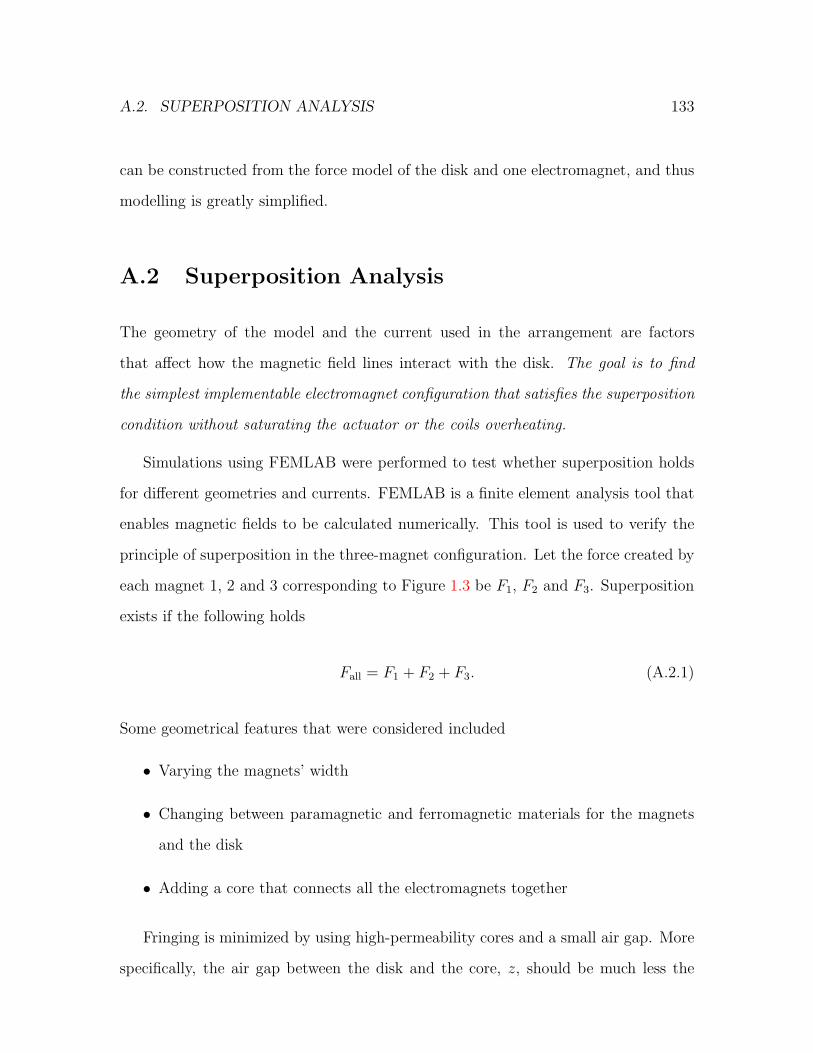
A.2. SUPERPOSITION ANALYSIS 133
can be constructed from the force model of the disk and one electromagnet, and thus
modelling is greatly simplified.
A.2 Superposition Analysis
The geometry of the model and the current used in the arrangement are factors
that affect how the magnetic field lines interact with the disk. The goal is to find
the simplest implementable electromagnet configuration that satisfies the superposition
condition without saturating the actuator or the coils overheating.
Simulations using FEMLAB were performed to test whether superposition holds
for different geometries and currents. FEMLAB is a finite element analysis tool that
enables magnetic fields to be calculated numerically. This tool is used to verify the
principle of superposition in the three-magnet configuration. Let the force created by
each magnet 1, 2 and 3 corresponding to Figure 1.3 be F1, F2 and F3. Superposition
exists if the following holds
Fall = F1 + F2 + F3. (A.2.1)
Some geometrical features that were considered included
• Varying the magnets’ width
• Changing between paramagnetic and ferromagnetic materials for the magnets
and the disk
• Adding a core that connects all the electromagnets together
Fringing is minimized by using high-permeability cores and a small air gap. More
specifically, the air gap between the disk and the core, z, should be much less the

A.2. SUPERPOSITION ANALYSIS 134
width of the core, w, and the height of the core, h [13]. Narrow magnets result in
a small width to air gap ratio, wz, and therefore allows for much fringing. Figure
A.2 demonstrates this model. The arrows on the plane represents the magnetic flux
density. Because of excess fringing, it was found through simulation that the condition
for superposition is not satisfied for narrow magnets.
Figure A.2: Magnetic flux density plot for narrow magnets.
Making the magnets wider to increase the wz
relationship minimizes fringing and
results in condition (A.2.1) being satisfied. See Figure A.3 for the magnetic flux
density line plot of the model.
The potential problem of the previous case is the area where superposition holds
may not be large. This would minimize the distance the disk can travel and would
therefore restrict testing of the controller. Although no simulations were ran to verify
this, increasing the width of the magnets should expand the region where super-
positon holds. Figure A.4 shows this arrangement. The results from each of these

A.2. SUPERPOSITION ANALYSIS 135
Figure A.3: Magnetic flux density plot for wide magnets.
configurations is shown later.
The material of the magnets and disk was chosen to be ferromagnetic because it
is the most widely used material for electromagnets. In particular, iron was chosen in
the simulations. Using a ferromagnetic material for the core of a magnet wrapped in
coils generates a magnetic field whose intensity is unmatched by other conventional
paramagnetic materials. Using a permanent magnet as the core strengthens the field
generated but complicates the model without improving superposition.
The final geometrical feature investigated entails adding a ferromagnetic core that
connected all the electromagnets together. This strengthens the magnetic fields pro-
duced by each magnet but complicates the model. Superposition with a reasonable
current can be achieved without the core.
Current, although not a geometrical feature, is another element of the model that
was considered. It is desired to keep current at a minimum to prevent the magnet’s
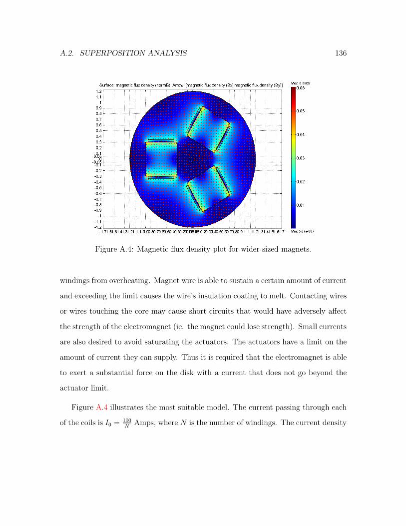
A.2. SUPERPOSITION ANALYSIS 136
Figure A.4: Magnetic flux density plot for wider sized magnets.
windings from overheating. Magnet wire is able to sustain a certain amount of current
and exceeding the limit causes the wire’s insulation coating to melt. Contacting wires
or wires touching the core may cause short circuits that would have adversely affect
the strength of the electromagnet (ie. the magnet could lose strength). Small currents
are also desired to avoid saturating the actuators. The actuators have a limit on the
amount of current they can supply. Thus it is required that the electromagnet is able
to exert a substantial force on the disk with a current that does not go beyond the
actuator limit.
Figure A.4 illustrates the most suitable model. The current passing through each
of the coils is I0 = 100N
Amps, where N is the number of windings. The current density
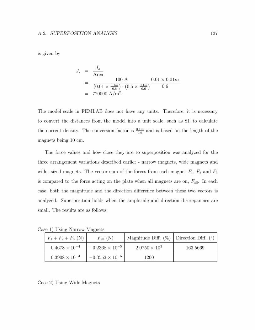
A.2. SUPERPOSITION ANALYSIS 137
is given by
Js =Io
Area
=100 A
(
0.01 × 0.1m0.6
)
·(
0.5 × 0.1m0.6
)
0.01 × 0.01m
0.6
= 720000 A/m2.
The model scale in FEMLAB does not have any units. Therefore, it is necessary
to convert the distances from the model into a unit scale, such as SI, to calculate
the current density. The conversion factor is 0.1m0.6
and is based on the length of the
magnets being 10 cm.
The force values and how close they are to superposition was analyzed for the
three arrangement variations described earlier - narrow magnets, wide magnets and
wider sized magnets. The vector sum of the forces from each magnet F1, F2 and F3
is compared to the force acting on the plate when all magnets are on, Fall. In each
case, both the magnitude and the direction difference between these two vectors is
analyzed. Superposition holds when the amplitude and direction discrepancies are
small. The results are as follows
Case 1) Using Narrow Magnets
F1 + F2 + F3 (N) Fall (N) Magnitude Diff. (%) Direction Diff. (o)
0.4678 × 10⁻⁴ −0.2368 × 10⁻⁵ 2.0750 × 10³ 163.5669
0.3908 × 10⁻⁴ −0.3553 × 10⁻⁵ 1200
Case 2) Using Wide Magnets

A.2. SUPERPOSITION ANALYSIS 138
F1 + F2 + F3 (N) Fall (N) Magnitude Diff. (%) Direction Diff. (o)
−0.9355 × 10⁻⁴ 0 0.0000 0.0000
−0.7283 × 10⁻⁴ 0 0.0000
Case 3) Using Wider Magnets
F1 + F2 + F3 (N) Fall (N) Magnitude Diff. (%) Direction Diff. (o)
0.4619 × 10⁻⁴ 0 0.0000 0.0000
−0.5684 × 10⁻⁴ 0 0.0000
In conclusion, superposition holds in case 2 and case 3. Although not tested, the
wider magnet model probably results in a larger region where superposition holds.
Therefore, case 3 is chosen as the best configuration for the implementation. However,
the force exerted on the disk by the magnets becomes smaller as the width of magnets
is increased. Thus, the size of the superposition region may have to be sacrificed so
that low currents can provide a sufficient force to move the disk without saturating
any of the cores or going over the magnet wire’s current threshold. The dimensions
of the cores chosen for implementation will be explained in Chapter 4.

Bibliography
[1] Kenneth D. Demarest. Engineering Electromagnetics. Prentice Hall, New Jersey,
1998. 2.1, 2.1, 2.1, 2.4, 4.1.1, 4.2.1, 4.2.1
[2] Hassan K. Khalil. Nonlinear Systems. Prentice Hall, Upper Saddle River, NJ
07458, second edition, 1995. 3.2
[3] John D. Kraus. Electromagnetics. McGraw-Hill, Inc., New York, 1992. 2.1
[4] Miroslav Krstic, Ioannis Kanellakopoulos, and Petar Kokotovic. Nonlinear and
Adaptive Control Design. John Wiley & Sons, Inc., 605 Third Avenue, New
York, NY, first edition, 1995. 3.3, 3.3.1, 3.3.1
[5] Chin E. Lin and Ann-San Hou. Real-time position and attitude sensing using
ccd cameras in magnetic suspension system applications. IEEE Transactions on
Instrumentation and Measurement, 44:8–13, February 1995. 4.1.5
[6] M. M. Polycarpou and P. A. Ioannou. A robust adaptive nonlinear control design.
Automatica, 32:423–427, 1996. 3.4, 3.4.1, 3.4.1, 3.4.1
[7] Ximin Shan, Shih-Kang Kuo, Jihua Zhang, , and Chia-Hsiang Menq. Ultra
precision motion control of a multiple degrees of freedom magnetic suspension
stage. IEEE/ASME Transactions on Mechatronics, 7:67–78, 2002. 1.1
139

BIBLIOGRAPHY 140
[8] Benyamin Grosman Sivan Lachman-Shalem and Daniel R. Lewin. Nonlinear
modeling and multivariable control of photolithography. IEEE Transactions on
Semiconductor Manufacturing, 15:310–322, 2002. 1.1
[9] Jean-Jackques E. Slotline and Weiping Li. Applied Nonlinear Control. Prentice
Hall, Englewood Cliffs, NJ 07632, first edition, 1991. 3.2.1
[10] J.T. Spooner, M. Maggiore, R. Ordonez, and K.M. Passino. Stable Adaptive
Control and Estimation for Nonlinear Systems: Neural and Fuzzy Approximator
Techniques. John Wiley & Sons, New York, 2002. 3.1, 3.1, 4.3.1
[11] David L. Trumper. Modeling and vector control of planar magnetic levitator.
IEEE Transactions on Industry Applications, 34:1254–1262, 1998. 1.1
[12] Kuen-Yu Tsai and Jia-Yush Yen. Servo system design of a high-resolution piezo-
driven fine stage for step-and-repeat microlithography systems. The 25th Annual
Conference of the IEEE Industrial Electonics Society, 1:11–16, 1999. 1.1
[13] Herbert H. Woodson and James R. Melcher. Electromechanical Dynamics. John
Wiley & Sons, Inc., New York, 1968. 2.1, 2.1, 4.2.1, A.2