nonlinear observer design for gnss and imu integration
TRANSCRIPT
Master of Science in Engineering CyberneticsJune 2011Thor Inge Fossen, ITK
Submission date:Supervisor:
Norwegian University of Science and TechnologyDepartment of Engineering Cybernetics
Nonlinear Observer Design for GNSSand IMU Integration
Harald Nøkland

Nonlinear Observer Design forGNSS and IMU Integration
Harald NøklandJune 2011
Master’s Thesis for the Degree ofMSc in Engineering Cybernetics
Department of Engineering CyberneticsFaculty of Information Technology,Mathematics and Electrical EngineeringNorwegian University of Science and Technology

ii
NTNU Faculty of Information Technology, Norwegian University of Mathematics and Electrical Engineering Science and Technology Department of Engineering Cybernetics
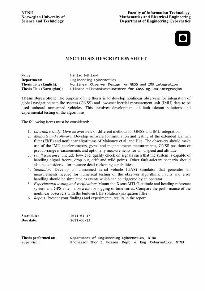
MSC THESIS DESCRIPTION SHEET
Name: Harlad Nøkland Department: Engineering Cybernetics Thesis Title (English): Nonlinear Observer Design for GNSS and IMU integration Thesis Title (Norwegian): Ulinære tilstandsestimatorer for GNSS og IMU integrasjon Thesis Description: The purpose of the thesis is to develop nonlinear observers for integration of global navigation satellite system (GNSS) and low-cost inertial measurement unit (IMU) data to be used onboard unmanned vehicles. This involves development of fault-tolerant solutions and experimental testing of the algorithms. The following items must be considered:
1. Literature study: Give an overview of different methods for GNSS and IMU integration. 2. Methods and software: Develop software for simulation and testing of the extended Kalman
filter (EKF) and nonlinear algorithms of Mahoney et al. and Hua. The observers should make use of the IMU accelerometers, gyros and magnetometer measurements, GNSS positions or pseudo-range measurements and optionally measurements for wind speed and altitude.
3. Fault tolerance: Include low-level quality check on signals such that the system is capable of handling signal freeze, drop out, drift and wild points. Other fault-tolerant scenario should also be considered, for instance dead-reckoning capabilities.
4. Simulator: Develop an unmanned aerial vehicle (UAS) simulator that generates all measurements needed for numerical testing of the observer algorithms. Faults and error handling should be simulated as events which can be triggered by an operator.
5. Experimental testing and verification: Mount the Xsens MTi-G attitude and heading reference system and GPS antenna on a car for logging of time-series. Compare the performance of the nonlinear observers with the build-in EKF solution (navigation filter).
6. Report: Present your findings and experimental results in the report.
Start date: 2011-‐01-‐17 Due date: 2011-‐06-‐13 Thesis performed at: Department of Engineering Cybernetics, NTNU Supervisor: Professor Thor I. Fossen, Dept. of Eng. Cybernetics, NTNU

iv
Abstract
In order to efficiently control an unmanned vehicle, knowledge about the position,velocity and attitude (orientation) is needed. This thesis address this problem,and designs a navigation system for local navigation using low-cost sensors. Twoloosely coupled GNSS/IMU integration filters are developed using a direct stateestimation approach.
The first is a quaternion based multiplicative extended Kalman filter (MEKF). Amultiplicative filter differs from the usual EKF in how the attitude is represented,which is done by a quaternion product. The filter avoids the singular covariancematrix caused by the constraint on the quaternion. Two versions of the filter aredeveloped: one using the q-method to get a measurement of the attitude; and oneusing vector measurements directly.
The second is a nonlinear observer, termed HuaMahony. It is derived by combiningtwo nonlinear algorithms proposed by Mahony et al. and Hua. The resultingnonlinear observer is able to estimate the linear acceleration as well as gyro bias.The nonlinear observer is written on an EKF-like discrete-time corrector-predictorformulation.
Both the multiplicative extended Kalman filter and the nonlinear observer aretested and verified through simulations and experimental data. Tests are carriedout to examine how different disturbances affects the estimates and to compare theperformance results.
Simulation results shows an average dynamic accuracy of <0.5 deg RMS for theattitude estimates, for both observers. The results from the experimental testsshows an average roll, pitch and yaw accuracy of (0.3 0.3 2.0) and (0.8 0.7 4.4)deg RMS for the MEKF and HuaMahony observer respectively, where it has beenassumed that the Xsens MTi-G built-in EKF estimates are the true values.
An advantage of the MEKF is quicker convergence from initial errors, while an ad-vantage of the HuaMahony observer is less computational load. Results show thatthe HuaMahony is three times faster than the MEKF when it comes to executiontime.
v

vi

Preface
This thesis is the final work of the Master of Science (MSc) program provided bythe Norwegian University of Science and Technology (NTNU). It has been carriedout at the Department of Engineering Cybernetics (ITK).
I would like to thank my supervisor professor Thor I. Fossen for his guidance. AlsoI would like to thank my brother Arild Nøkland for many valuable discussions.Finally, I would like to thank my fellow student Jakob Jakobsen for lending me theXsens MTi-G unit, which have been used to record experimental data.
Harald NøklandTrondheim, June 2011
vii

viii
Contents
1 Introduction 1
1.1 Motivation . . . . . . . . . . . . . . . . . . . . . . . . . . . . . . . . 1
1.2 State-of-the-Art Navigation Systems . . . . . . . . . . . . . . . . . . 2
1.2.1 Attitude Aiding . . . . . . . . . . . . . . . . . . . . . . . . . . 2
1.2.2 Position and Velocity Aiding . . . . . . . . . . . . . . . . . . 3
1.2.3 Direct and Indirect Integration . . . . . . . . . . . . . . . . . 3
1.2.4 Integration Filter . . . . . . . . . . . . . . . . . . . . . . . . . 4
1.3 This Thesis . . . . . . . . . . . . . . . . . . . . . . . . . . . . . . . . 4
1.4 Contributions . . . . . . . . . . . . . . . . . . . . . . . . . . . . . . . 5
2 Background 7
2.1 Reference Frames . . . . . . . . . . . . . . . . . . . . . . . . . . . . . 7
2.2 Notation . . . . . . . . . . . . . . . . . . . . . . . . . . . . . . . . . . 8
2.3 Transformation between BODY and NED . . . . . . . . . . . . . . . 9
2.3.1 Quaternion Differential Equation . . . . . . . . . . . . . . . . 10
2.4 Transformation between NED and ECEF . . . . . . . . . . . . . . . 10
2.4.1 Transformation from Cartesian to Ellipsoidal ECEF Coordi-nates . . . . . . . . . . . . . . . . . . . . . . . . . . . . . . . . 11
2.4.2 Transformation from Ellipsoidal to Cartesian ECEF Coordi-nates . . . . . . . . . . . . . . . . . . . . . . . . . . . . . . . . 12
2.5 Transformation between ECEF and ECI . . . . . . . . . . . . . . . . 12
ix
x CONTENTS
3 Sensor and Navigation Systems 13
3.1 Inertial Measurement Unit (IMU) . . . . . . . . . . . . . . . . . . . . 13
3.1.1 Gyro measurement . . . . . . . . . . . . . . . . . . . . . . . . 14
3.1.2 Gyro error model . . . . . . . . . . . . . . . . . . . . . . . . . 14
3.1.3 Accelerometer measurement . . . . . . . . . . . . . . . . . . . 14
3.1.4 Accelerometer error model . . . . . . . . . . . . . . . . . . . . 15
3.1.5 Magnetometer measurement . . . . . . . . . . . . . . . . . . . 15
3.1.6 Magnetometer error model . . . . . . . . . . . . . . . . . . . 16
3.2 Global Positioning System (GPS) . . . . . . . . . . . . . . . . . . . . 16
3.2.1 NED Coordinates from Longitude and Latitude . . . . . . . 16
3.2.2 GPS error model . . . . . . . . . . . . . . . . . . . . . . . . . 17
3.3 Xsens MTi-G . . . . . . . . . . . . . . . . . . . . . . . . . . . . . . . 17
3.3.1 Configuration . . . . . . . . . . . . . . . . . . . . . . . . . . . 18
3.3.2 Exporting Data . . . . . . . . . . . . . . . . . . . . . . . . . . 18
4 The q-method 21
4.1 Derivation of the q-method algorithm . . . . . . . . . . . . . . . . . 21
4.2 Using the q-method . . . . . . . . . . . . . . . . . . . . . . . . . . . 24
5 Extended Kalman Filter Design 27
5.1 Discrete Multiplicative Extended Kalman Filter . . . . . . . . . . . . 28
5.2 Attitude Estimation . . . . . . . . . . . . . . . . . . . . . . . . . . . 28
5.2.1 Assumptions . . . . . . . . . . . . . . . . . . . . . . . . . . . 30
5.2.2 Attitude Model . . . . . . . . . . . . . . . . . . . . . . . . . . 30
5.2.3 Measurement Equation . . . . . . . . . . . . . . . . . . . . . 32
5.2.4 Discrete-Time Matrices . . . . . . . . . . . . . . . . . . . . . 32
5.2.5 Alternative Measurement Equation . . . . . . . . . . . . . . . 33
5.3 Position, Velocity and Attitude Estimation . . . . . . . . . . . . . . 34
5.3.1 Assumptions . . . . . . . . . . . . . . . . . . . . . . . . . . . 34
5.3.2 Position, Velocity and Attitude Models . . . . . . . . . . . . 34
5.3.3 Measurement Equation . . . . . . . . . . . . . . . . . . . . . 34
5.3.4 Discrete-Time Matrices . . . . . . . . . . . . . . . . . . . . . 35
5.3.5 Alternative Measurement Equation . . . . . . . . . . . . . . . 36
CONTENTS xi
6 Nonlinear Observer Design 396.1 Attitude Observer . . . . . . . . . . . . . . . . . . . . . . . . . . . . 39
6.1.1 Discrete-Time Corrector-Predictor Formulation . . . . . . . . 406.2 Position, Velocity and Attitude Observer . . . . . . . . . . . . . . . . 41
6.2.1 Discrete-Time Corrector-Predictor Formulation . . . . . . . . 42
7 Simulator 457.1 Simulator Model . . . . . . . . . . . . . . . . . . . . . . . . . . . . . 457.2 Simulator Parameters and Measurement Noise . . . . . . . . . . . . 46
8 Implementation 498.1 Numerical Properties of Different Attitude Representations . . . . . 498.2 Using the q-method . . . . . . . . . . . . . . . . . . . . . . . . . . . 508.3 Saturation for δε . . . . . . . . . . . . . . . . . . . . . . . . . . . . . 508.4 Dead-reckoning . . . . . . . . . . . . . . . . . . . . . . . . . . . . . . 518.5 Low-Level Signal Check . . . . . . . . . . . . . . . . . . . . . . . . . 518.6 Magnetic Distortion Compensation . . . . . . . . . . . . . . . . . . . 53
9 Simulation Results 559.1 Description of Case Studies . . . . . . . . . . . . . . . . . . . . . . . 569.2 Case 1: Perfect Data . . . . . . . . . . . . . . . . . . . . . . . . . . 609.3 Case 2: Noise Only . . . . . . . . . . . . . . . . . . . . . . . . . . . . 609.4 Case 3: Gyro Bias . . . . . . . . . . . . . . . . . . . . . . . . . . . . 609.5 Case 4: Local Magnetic Disturbance . . . . . . . . . . . . . . . . . . 619.6 Case 5: Accelerometer Bias . . . . . . . . . . . . . . . . . . . . . . . 629.7 Case 6: Variable Force . . . . . . . . . . . . . . . . . . . . . . . . . . 62
10 Experimental Results 6510.1 Main Results . . . . . . . . . . . . . . . . . . . . . . . . . . . . . . . 6810.2 Lever Arm Compensation . . . . . . . . . . . . . . . . . . . . . . . . 6910.3 Initial error . . . . . . . . . . . . . . . . . . . . . . . . . . . . . . . . 7010.4 Linear Accelerations . . . . . . . . . . . . . . . . . . . . . . . . . . . 7110.5 Measurement Equation . . . . . . . . . . . . . . . . . . . . . . . . . . 7210.6 Execution Time . . . . . . . . . . . . . . . . . . . . . . . . . . . . . . 7210.7 GPS Outage . . . . . . . . . . . . . . . . . . . . . . . . . . . . . . . . 73

xii CONTENTS
11 Conclusions 75
12 Further Work 77
Bibliography 79
A Matlab Code 83
A.1 Multiplicative Extended Kalman Filter . . . . . . . . . . . . . . . . . 83
A.2 Multiplicative Extended Kalman Filter (q-method) . . . . . . . . . . 86
A.3 Nonlinear Observer HuaMahony . . . . . . . . . . . . . . . . . . . . 88
A.4 q-method . . . . . . . . . . . . . . . . . . . . . . . . . . . . . . . . . 90
B Simulink Diagrams 91
C CD Content 95
Chapter 1
Introduction
Today all sorts of unmanned vehicles are becoming increasingly popular. Applica-tions include data acquisition, surveillance or hazardous missions without the riskof human lives. Currently it is widely used for military purposes, however a greatpotential also exist for civilian or research purposes.
In order to efficiently control an unmanned vehicle, knowledge about the posi-tion, velocity and attitude (orientation) is needed. This is generally provided by anavigation system, however commercial high-quality navigation systems are ratherexpensive. This motivates the development of a navigation system using low-costsensors. Typical inertial sensors that are used for navigation purposes are ac-celerometers, gyros and magnetometers. Together they form an inertial measure-ment unit (IMU). In addition, global navigation satellite systems (GNSS) are oftenused, such as GPS.
1.1 Motivation
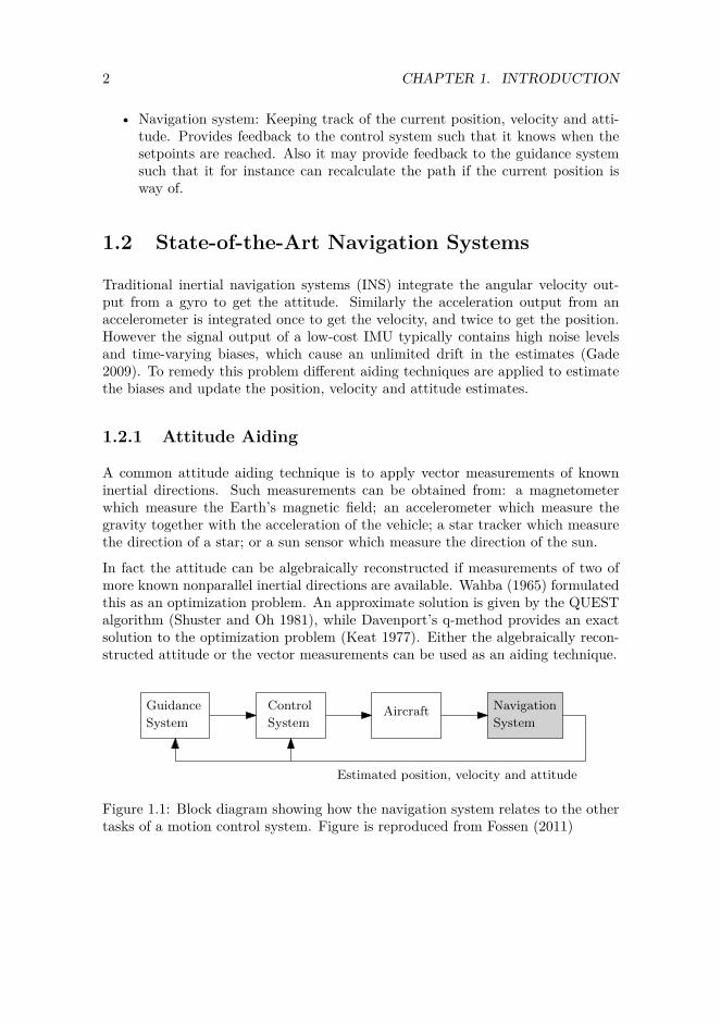
The purpose of this thesis is to develop a GNSS/IMU integrated navigation system,using a low-cost IMU. It is to be used onboard an unmanned aerial vehicle (UAV)in order to provide estimates of position, velocity and attitude. It is an importantpart of a motion control system, which usually is divided into the following tasks(see Figure 1.1):
• Guidance system: Path planning and trajectory generation, providing set-points to the control system.
• Control system: Manipulating the actuators such that the setpoints arereached.
1
2 CHAPTER 1. INTRODUCTION
• Navigation system: Keeping track of the current position, velocity and atti-tude. Provides feedback to the control system such that it knows when thesetpoints are reached. Also it may provide feedback to the guidance systemsuch that it for instance can recalculate the path if the current position isway of.
1.2 State-of-the-Art Navigation Systems
Traditional inertial navigation systems (INS) integrate the angular velocity out-put from a gyro to get the attitude. Similarly the acceleration output from anaccelerometer is integrated once to get the velocity, and twice to get the position.However the signal output of a low-cost IMU typically contains high noise levelsand time-varying biases, which cause an unlimited drift in the estimates (Gade2009). To remedy this problem different aiding techniques are applied to estimatethe biases and update the position, velocity and attitude estimates.
1.2.1 Attitude Aiding
A common attitude aiding technique is to apply vector measurements of knowninertial directions. Such measurements can be obtained from: a magnetometerwhich measure the Earth’s magnetic field; an accelerometer which measure thegravity together with the acceleration of the vehicle; a star tracker which measurethe direction of a star; or a sun sensor which measure the direction of the sun.
In fact the attitude can be algebraically reconstructed if measurements of two ofmore known nonparallel inertial directions are available. Wahba (1965) formulatedthis as an optimization problem. An approximate solution is given by the QUESTalgorithm (Shuster and Oh 1981), while Davenport’s q-method provides an exactsolution to the optimization problem (Keat 1977). Either the algebraically recon-structed attitude or the vector measurements can be used as an aiding technique.
AircraftControlGuidance Navigation
System System System
Estimated position, velocity and attitude
Figure 1.1: Block diagram showing how the navigation system relates to the othertasks of a motion control system. Figure is reproduced from Fossen (2011)
1.2. STATE-OF-THE-ART NAVIGATION SYSTEMS 3
1.2.2 Position and Velocity Aiding
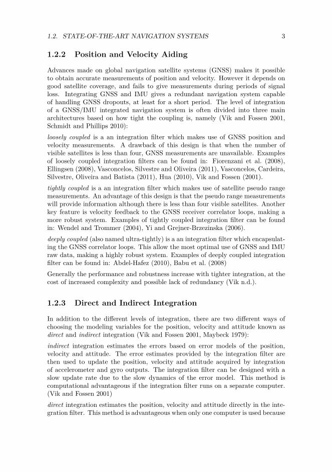
Advances made on global navigation satellite systems (GNSS) makes it possibleto obtain accurate measurements of position and velocity. However it depends ongood satellite coverage, and fails to give measurements during periods of signalloss. Integrating GNSS and IMU gives a redundant navigation system capableof handling GNSS dropouts, at least for a short period. The level of integrationof a GNSS/IMU integrated navigation system is often divided into three mainarchitectures based on how tight the coupling is, namely (Vik and Fossen 2001,Schmidt and Phillips 2010):loosely coupled is a an integration filter which makes use of GNSS position andvelocity measurements. A drawback of this design is that when the number ofvisible satellites is less than four, GNSS measurements are unavailable. Examplesof loosely coupled integration filters can be found in: Fiorenzani et al. (2008),Ellingsen (2008), Vasconcelos, Silvestre and Oliveira (2011), Vasconcelos, Cardeira,Silvestre, Oliveira and Batista (2011), Hua (2010), Vik and Fossen (2001).tightly coupled is a an integration filter which makes use of satellite pseudo rangemeasurements. An advantage of this design is that the pseudo range measurementswill provide information although there is less than four visible satellites. Anotherkey feature is velocity feedback to the GNSS receiver correlator loops, making amore robust system. Examples of tightly coupled integration filter can be foundin: Wendel and Trommer (2004), Yi and Grejner-Brzezinska (2006).deeply coupled (also named ultra-tightly) is a an integration filter which encapsulat-ing the GNSS correlator loops. This allow the most optimal use of GNSS and IMUraw data, making a highly robust system. Examples of deeply coupled integrationfilter can be found in: Abdel-Hafez (2010), Babu et al. (2008)Generally the performance and robustness increase with tighter integration, at thecost of increased complexity and possible lack of redundancy (Vik n.d.).
1.2.3 Direct and Indirect Integration
In addition to the different levels of integration, there are two different ways ofchoosing the modeling variables for the position, velocity and attitude known asdirect and indirect integration (Vik and Fossen 2001, Maybeck 1979):indirect integration estimates the errors based on error models of the position,velocity and attitude. The error estimates provided by the integration filter arethen used to update the position, velocity and attitude acquired by integrationof accelerometer and gyro outputs. The integration filter can be designed with aslow update rate due to the slow dynamics of the error model. This method iscomputational advantageous if the integration filter runs on a separate computer.(Vik and Fossen 2001)direct integration estimates the position, velocity and attitude directly in the inte-gration filter. This method is advantageous when only one computer is used because
4 CHAPTER 1. INTRODUCTION
it avoids the additional propagation of an error model. However, if a Kalman filteris used for integration, the indirect method may still be more efficient, as a highupdate rate of the covariance matrix is computational intensive. (Vik and Fossen2001)
1.2.4 Integration Filter
The the body-fixed measurements of angular velocity and acceleration is relatedto the position, velocity and attitude through differential equations, known as thestrapdown inertial navigation equations (Vik n.d.). The equations are nonlinear,thus nonlinear algorithms are most suitable for integration of GNSS and IMU.Usually an extended Kalman filter (EKF) is used, but other methods are alsoused.
A survey of modern nonlinear attitude estimation methods is presented in Cras-sidis et al. (2007). There has recently been an increasingly interest for nonlinearobservers (Vik and Fossen 2001, Mahony et al. 2008, Martin and Salaün 2008, Hua2010, Fossen 2011, Vasconcelos, Cardeira, Silvestre, Oliveira and Batista 2011).Nonlinear observers offer an easier to tune and less computational alternative tothe EKF. In addition stronger proofs of stability and convergence can be achieved.
1.3 This Thesis
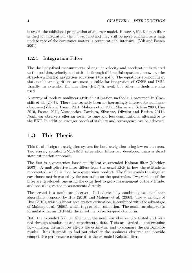
This thesis designs a navigation system for local navigation using low-cost sensors.Two loosely coupled GNSS/IMU integration filters are developed using a directstate estimation approach.
The first is a quaternion based multiplicative extended Kalman filter (Markley2003). A multiplicative filter differs from the usual EKF in how the attitude isrepresented, which is done by a quaternion product. The filter avoids the singularcovariance matrix caused by the constraint on the quaternion. Two versions of thefilter are developed: one using the q-method to get a measurement of the attitude;and one using vector measurements directly.
The second is a nonlinear observer. It is derived by combining two nonlinearalgorithms proposed by Hua (2010) and Mahony et al. (2008). The advantage ofHua (2010), which is linear acceleration estimation, is combined with the advantageof Mahony et al. (2008), which is gyro bias estimation. The nonlinear observer isformulated on an EKF-like discrete-time corrector-predictor form.
Both the extended Kalman filter and the nonlinear observer are tested and veri-fied through simulations and experimental data. Tests are carried out to examinehow different disturbances affects the estimates. and to compare the performanceresults. It is desirable to find out whether the nonlinear observer can providecompetitive performance compared to the extended Kalman filter.
1.4. CONTRIBUTIONS 5
1.4 Contributions
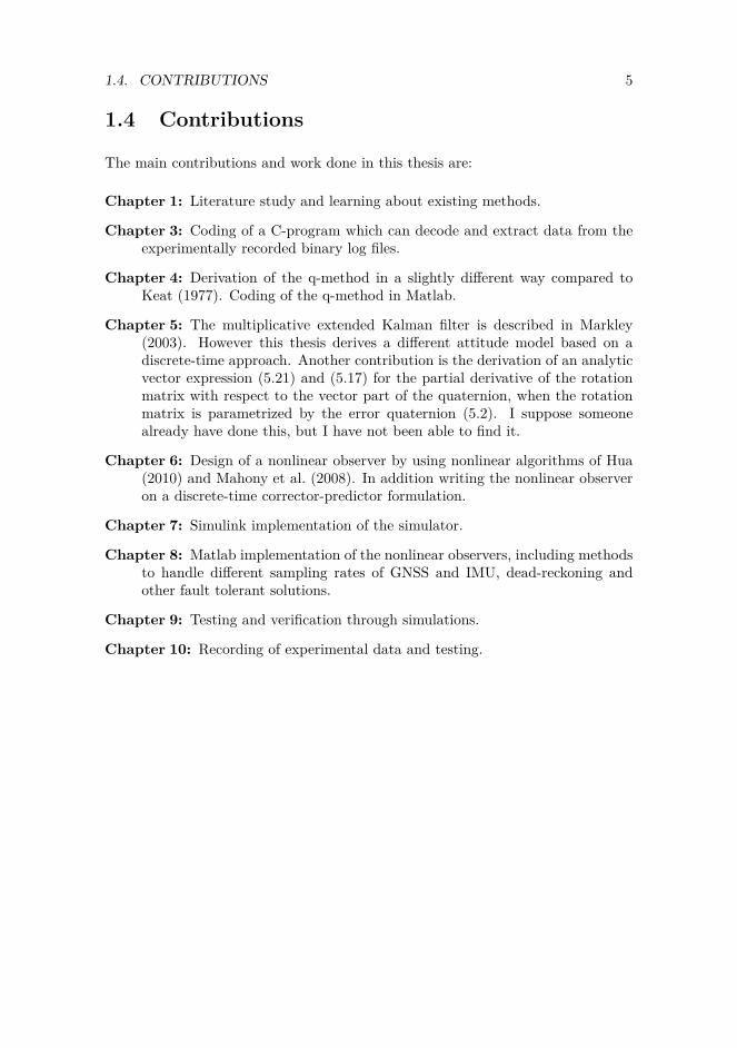
The main contributions and work done in this thesis are:
Chapter 1: Literature study and learning about existing methods.
Chapter 3: Coding of a C-program which can decode and extract data from theexperimentally recorded binary log files.
Chapter 4: Derivation of the q-method in a slightly different way compared toKeat (1977). Coding of the q-method in Matlab.
Chapter 5: The multiplicative extended Kalman filter is described in Markley(2003). However this thesis derives a different attitude model based on adiscrete-time approach. Another contribution is the derivation of an analyticvector expression (5.21) and (5.17) for the partial derivative of the rotationmatrix with respect to the vector part of the quaternion, when the rotationmatrix is parametrized by the error quaternion (5.2). I suppose someonealready have done this, but I have not been able to find it.
Chapter 6: Design of a nonlinear observer by using nonlinear algorithms of Hua(2010) and Mahony et al. (2008). In addition writing the nonlinear observeron a discrete-time corrector-predictor formulation.
Chapter 7: Simulink implementation of the simulator.
Chapter 8: Matlab implementation of the nonlinear observers, including methodsto handle different sampling rates of GNSS and IMU, dead-reckoning andother fault tolerant solutions.
Chapter 9: Testing and verification through simulations.
Chapter 10: Recording of experimental data and testing.

6 CHAPTER 1. INTRODUCTION
Chapter 2
Background
This chapter contains a brief summary of navigation fundamentals. This is basedon Fossen (2011) and Vik (n.d.).
2.1 Reference Frames
The different reference frames used here are described as follows:
ECI
The Earth-Centered Inertial (ECI) frame i = (xi, yi, zi) is an inertial frame fixedin space. The origin of i is located at the center of the Earth. It is defined withthe x-axis pointing towards the vernal equinox, and the z-axis pointing along theEarth’s rotation axis. The y-axis completes the right handed orthogonal coordinatesystem.
ECEF
The Earth-Centered Earth-Fixed (ECEF) frame e = (xe, ye, ze) has its originfixed to the center of the Earth. It is defined with the x-axis pointing towardsthe intersection of 0 longitude (Greenwich meridian) and 0 latitude (Equator).The z-axis points along the Earth’s rotation axis, and the y-axis complete the righthanded orthogonal coordinate system. The ECEF frame rotates relative to the ECIframe with the Earth rotation rate ωe = 7.2921 · 10−5 rad/s. Both Cartesian andellipsoidal coordinates (longitude, latitude, height) are used to represent positionin the ECEF frame.
7
8 CHAPTER 2. BACKGROUND
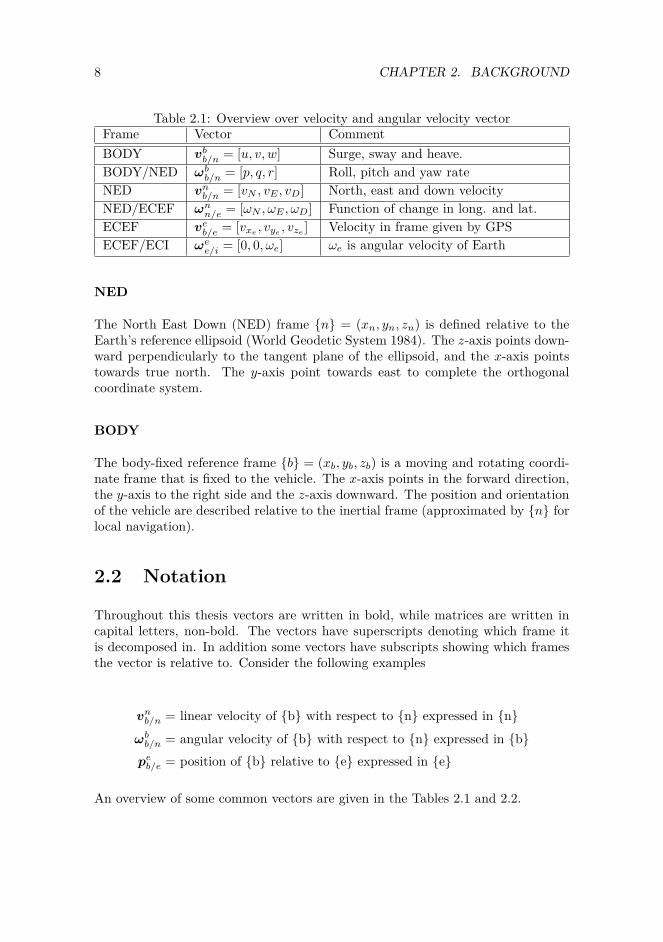
Table 2.1: Overview over velocity and angular velocity vectorFrame Vector CommentBODY vbb/n = [u, v, w] Surge, sway and heave.BODY/NED ωbb/n = [p, q, r] Roll, pitch and yaw rateNED vnb/n = [vN , vE , vD] North, east and down velocityNED/ECEF ωnn/e = [ωN , ωE , ωD] Function of change in long. and lat.ECEF veb/e = [vxe
, vye, vze
] Velocity in frame given by GPSECEF/ECI ωee/i = [0, 0, ωe] ωe is angular velocity of Earth
NED
The North East Down (NED) frame n = (xn, yn, zn) is defined relative to theEarth’s reference ellipsoid (World Geodetic System 1984). The z-axis points down-ward perpendicularly to the tangent plane of the ellipsoid, and the x-axis pointstowards true north. The y-axis point towards east to complete the orthogonalcoordinate system.
BODY
The body-fixed reference frame b = (xb, yb, zb) is a moving and rotating coordi-nate frame that is fixed to the vehicle. The x-axis points in the forward direction,the y-axis to the right side and the z-axis downward. The position and orientationof the vehicle are described relative to the inertial frame (approximated by n forlocal navigation).
2.2 Notation
Throughout this thesis vectors are written in bold, while matrices are written incapital letters, non-bold. The vectors have superscripts denoting which frame itis decomposed in. In addition some vectors have subscripts showing which framesthe vector is relative to. Consider the following examples
vnb/n = linear velocity of b with respect to n expressed in n
ωbb/n = angular velocity of b with respect to n expressed in bpeb/e = position of b relative to e expressed in e
An overview of some common vectors are given in the Tables 2.1 and 2.2.
2.3. TRANSFORMATION BETWEEN BODY AND NED 9
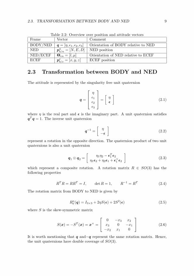
Table 2.2: Overview over position and attitude vectorsFrame Vector CommentBODY/NED q = [η, ε1, ε2, ε3] Orientation of BODY relative to NEDNED pnb/n = [N,E,D] NED positionNED/ECEF Θen = [l, µ] Orientation of NED relative to ECEFECEF peb/e = [x, y, z] ECEF position
2.3 Transformation between BODY and NED
The attitude is represented by the singularity free unit quaternion
q =
ηε1ε2ε3
=[ηε
](2.1)
where η is the real part and ε is the imaginary part. A unit quaternion satisfiesqTq = 1. The inverse unit quaternion
q−1 =[
η−ε
](2.2)
represent a rotation in the opposite direction. The quaternion product of two unitquaternions is also a unit quaternion
q1 ⊗ q2 =[
η1η2 − εT1 ε2η1ε2 + η2ε1 + ε×1 ε2
](2.3)
which represent a composite rotation. A rotation matrix R ∈ SO(3) has thefollowing properties
RTR = RRT = I, detR = 1, R−1 = RT (2.4)
The rotation matrix from BODY to NED is given by
Rnb (q) = I3×3 + 2ηS(ε) + 2S2(ε) (2.5)
where S is the skew-symmetric matrix
S(x) = −ST (x) = x× =
0 −x3 x2x3 0 −x1−x2 x1 0
(2.6)
It is worth mentioning that q and−q represent the same rotation matrix. Hence,the unit quaternions have double coverage of SO(3).
10 CHAPTER 2. BACKGROUND
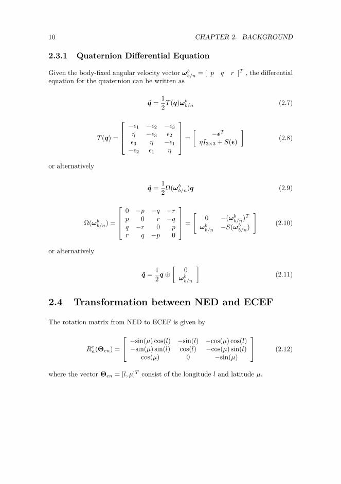
2.3.1 Quaternion Differential Equation
Given the body-fixed angular velocity vector ωbb/n = [ p q r ]T , the differentialequation for the quaternion can be written as
q = 12T (q)ωbb/n (2.7)
T (q) =
−ε1 −ε2 −ε3η −ε3 ε2ε3 η −ε1−ε2 ε1 η
=[
−εTηI3×3 + S(ε)
](2.8)
or alternatively
q = 12Ω(ωbb/n)q (2.9)
Ω(ωbb/n) =
0 −p −q −rp 0 r −qq −r 0 pr q −p 0
=[
0 −(ωbb/n)Tωbb/n −S(ωbb/n)
](2.10)
or alternatively
q = 12q ⊕
[0
ωbb/n
](2.11)
2.4 Transformation between NED and ECEF
The rotation matrix from NED to ECEF is given by
Ren(Θen) =
−sin(µ) cos(l) −sin(l) −cos(µ) cos(l)−sin(µ) sin(l) cos(l) −cos(µ) sin(l)
cos(µ) 0 −sin(µ)
(2.12)
where the vector Θen = [l, µ]T consist of the longitude l and latitude µ.
2.4. TRANSFORMATION BETWEEN NED AND ECEF 11
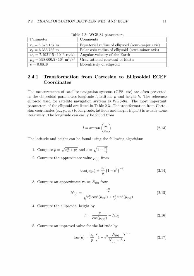
Table 2.3: WGS-84 parametersParameter Commentsre = 6 378 137 m Equatorial radius of ellipsoid (semi-major axis)rp = 6 356 752 m Polar axis radius of ellipsoid (semi-minor axis)ωe = 7.292115 · 10−5 rad/s Angular velocity of the Earthµg = 398 600.5 · 109 m3/s2 Gravitational constant of Earthe = 0.0818 Eccentricity of ellipsoid
2.4.1 Transformation from Cartesian to Ellipsoidal ECEFCoordinates
The measurements of satellite navigation systems (GPS, etc) are often presentedas the ellipsoidal parameters longitude l, latitude µ and height h. The referenceellipsoid used for satellite navigation systems is WGS-84. The most importantparameters of the ellipsoid are listed in Table 2.3. The transformation from Carte-sian coordinates (xe, ye, ze) to longitude, latitude and height (l, µ, h) is usually doneiteratively. The longitude can easily be found from
l = arctan(yexe
)(2.13)
The latitude and height can be found using the following algorithm:
1. Compute p =√x2e + y2
e and e =√
1− r2p
r2e
2. Compute the approximate value µ(0) from
tan(µ(0)) = zep
(1− e2)−1 (2.14)
3. Compute an approximate value N(0) from
N(0) = r2e√
r2e cos2(µ(0)) + r2
p sin2(µ(0))(2.15)
4. Compute the ellipsoidal height by
h = p
cos(µ(0))−N(0) (2.16)
5. Compute an improved value for the latitude by
tan(µ) = zep
(1− e2 N(0)
N(0) + h
)−1(2.17)
12 CHAPTER 2. BACKGROUND
6. Check for another iteration step: if µ = µ(0) then the iteration is completed.Otherwise set µ(0) = µ and continue with step 3.
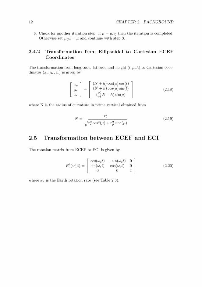
2.4.2 Transformation from Ellipsoidal to Cartesian ECEFCoordinates
The transformation from longitude, latitude and height (l, µ, h) to Cartesian coor-dinates (xe, ye, ze) is given by
xeyeze
=
(N + h) cos(µ) cos(l)(N + h) cos(µ) sin(l)
( r2p
r2eN + h) sin(µ)
(2.18)
where N is the radius of curvature in prime vertical obtained from
N = r2e√
r2e cos2(µ) + r2
p sin2(µ)(2.19)
2.5 Transformation between ECEF and ECI
The rotation matrix from ECEF to ECI is given by
Rie(ωeiet) =
cos(ωet) −sin(ωet) 0sin(ωet) cos(ωet) 0
0 0 1
(2.20)
where ωe is the Earth rotation rate (see Table 2.3).
Chapter 3
Sensor and NavigationSystems
Typical inertial sensors that are used for navigation purposes are accelerome-ters, gyros and magnetometers. Together they form an inertial measurement unit(IMU). In addition, global navigation satellite systems (GNSS) are often used.Several GNSS systems exists, such as GPS (American), GLONASS (Russian) andGALILEO (European). This chapter describes what the IMU and GPS measuresand the mathematical modeling of those measurements. The device used in thisthesis is the Xsens MTi-G unit (Xsens 2009d).
3.1 Inertial Measurement Unit (IMU)
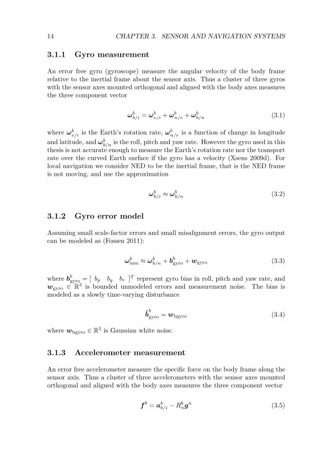
The IMU contains a cluster of three gyros, three accelerometers and three mag-netometers that measures angular velocity, acceleration and magnetic field respec-tively (see Figure 3.1).
abimu = [ax, ay, az]
TIMUAccelerometer
Gyro
Magnetometer
ωbimu = [ωx, ωy, ωz]
T
mbimu = [mx,my,mz]
T
Figure 3.1: Block diagram showing the IMU assembly and its signals.
13
14 CHAPTER 3. SENSOR AND NAVIGATION SYSTEMS
3.1.1 Gyro measurement
An error free gyro (gyroscope) measure the angular velocity of the body framerelative to the inertial frame about the sensor axis. Thus a cluster of three gyroswith the sensor axes mounted orthogonal and aligned with the body axes measuresthe three component vector
ωbb/i = ωbe/i + ωbn/e + ωbb/n (3.1)
where ωbe/i is the Earth’s rotation rate, ωbn/e is a function of change in longitudeand latitude, and ωbb/n is the roll, pitch and yaw rate. However the gyro used in thisthesis is not accurate enough to measure the Earth’s rotation rate nor the transportrate over the curved Earth surface if the gyro has a velocity (Xsens 2009d). Forlocal navigation we consider NED to be the inertial frame, that is the NED frameis not moving, and use the approximation
ωbb/i ≈ ωbb/n (3.2)
3.1.2 Gyro error model
Assuming small scale-factor errors and small misalignment errors, the gyro outputcan be modeled as (Fossen 2011):
ωbimu ≈ ωbb/n + bbgyro +wgyro (3.3)
where bbgyro = [ bp bq br ]T represent gyro bias in roll, pitch and yaw rate, andwgyro ∈ R3 is bounded unmodeled errors and measurement noise. The bias ismodeled as a slowly time-varying disturbance
bb
gyro = wbgyro (3.4)
where wbgyro ∈ R3 is Gaussian white noise.
3.1.3 Accelerometer measurement
An error free accelerometer measure the specific force on the body frame along thesensor axis. Thus a cluster of three accelerometers with the sensor axes mountedorthogonal and aligned with the body axes measures the three component vector
f b = abb/i −Rbng
n (3.5)
3.1. INERTIAL MEASUREMENT UNIT (IMU) 15
where abb/i is the linear acceleration of the moving body with respect to i ex-pressed in b, and gn ≈ [ 0 0 9, 81 ]T m/s2 is known as plumb bob gravity.For local navigation we consider NED to be the inertial frame, that is the NEDframe is not moving, and use the approximation
abb/i ≈ abb/n (3.6)
3.1.4 Accelerometer error model
Assuming small scale-factor errors and small misalignment errors, the accelerometeroutput can be modeled as (Fossen 2011):
f bimu ≈ abb/n −Rbng
n + bbacc +wacc (3.7)
or alternatively
f bimu ≈ Rbn[vnb/n − gn] + bbacc +wacc (3.8)
where bbacc = [ bu bv bw ]T represent accelerometer bias in x, y and z direction,and wacc ∈ R3 is bounded unmodeled errors and measurement noise. The bias ismodeled as a slowly time-varying disturbance
bb
acc = wbacc (3.9)
where wbacc ∈ R3 is Gaussian white noise.
3.1.5 Magnetometer measurement
An error free magnetometer measure the strength of the magnetic field along thesensor axis. Thus a cluster of three magnetometers with the sensor axes mountedorthogonal and aligned with the body axes measures the three component vector
mb = Rbnmn (3.10)
where mn = [ mN mE mD ]T represent the magnitude and direction of theEarth’s magnetic field. The magnetic field is different around the globe and infact time-varying as well. In our area (Trondheim, Norway) it is approximatelymn ≈ [ 13 605 439 49 864 ]T nT, which is found from an online calculator1.
1http://ngdc.noaa.gov/geomagmodels/IGRFWMM.jsp
16 CHAPTER 3. SENSOR AND NAVIGATION SYSTEMS
GPS
l, µ, h
vngps = [vN , vE , vD]T
pngps = [N,E,D]TTransform l, µ, h
to N,E,D
l0, µ0, h0
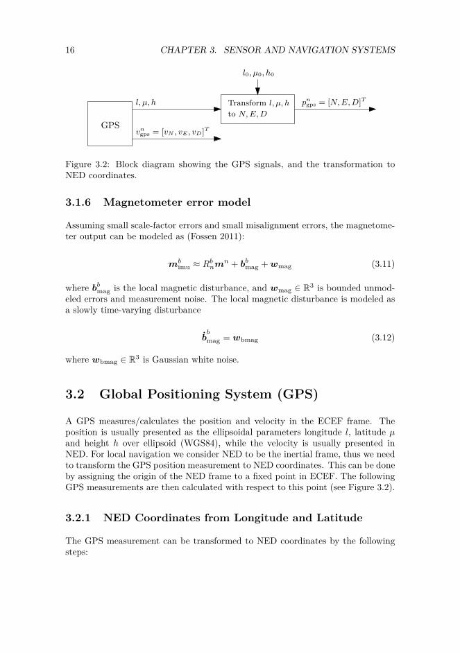
Figure 3.2: Block diagram showing the GPS signals, and the transformation toNED coordinates.
3.1.6 Magnetometer error model
Assuming small scale-factor errors and small misalignment errors, the magnetome-ter output can be modeled as (Fossen 2011):
mbimu ≈ Rbnmn + bbmag +wmag (3.11)
where bbmag is the local magnetic disturbance, and wmag ∈ R3 is bounded unmod-eled errors and measurement noise. The local magnetic disturbance is modeled asa slowly time-varying disturbance
bb
mag = wbmag (3.12)
where wbmag ∈ R3 is Gaussian white noise.
3.2 Global Positioning System (GPS)
A GPS measures/calculates the position and velocity in the ECEF frame. Theposition is usually presented as the ellipsoidal parameters longitude l, latitude µand height h over ellipsoid (WGS84), while the velocity is usually presented inNED. For local navigation we consider NED to be the inertial frame, thus we needto transform the GPS position measurement to NED coordinates. This can be doneby assigning the origin of the NED frame to a fixed point in ECEF. The followingGPS measurements are then calculated with respect to this point (see Figure 3.2).
3.2.1 NED Coordinates from Longitude and Latitude
The GPS measurement can be transformed to NED coordinates by the followingsteps:
3.3. XSENS MTI-G 17
1. Determine longitude, latitude and height of reference point (l0, µ0, h0) andcalculate the corresponding ECEF coordinates pe0 := pen/e by using (2.18).This will be the origin of the NED frame.
2. Transform the GPS measurement to ECEF coordinates peb/n by using (2.18)and calculate the displacement in NED by
pnb/n = Ren(l0, µ0)T [peb/e − pe0] (3.13)
3.2.2 GPS error model
Assuming that the GPS position measurement has been transformed to NED co-ordinates, the GPS output can be modeled as (Fossen 2011):
pngps = pnb/n +Rnb rbant +wpos (3.14)
vngps = vnb/n +Rnb S(ωbb/n)rbant +wvel (3.15)
where rbant is the location of the antenna andwpos,wvel ∈ R3 is bounded unmodelederrors and measurement noise.
3.3 Xsens MTi-G
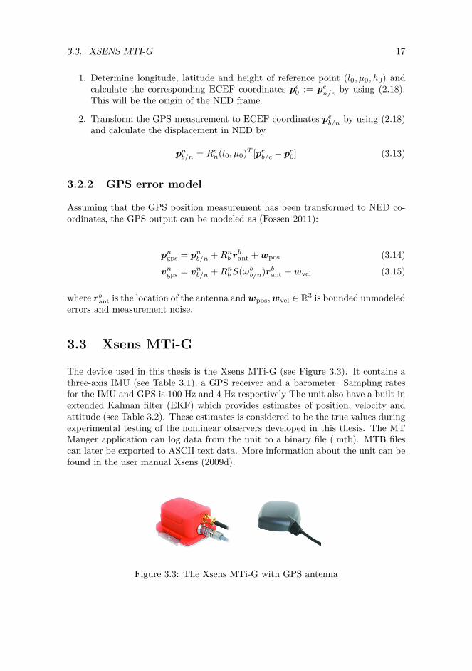
The device used in this thesis is the Xsens MTi-G (see Figure 3.3). It contains athree-axis IMU (see Table 3.1), a GPS receiver and a barometer. Sampling ratesfor the IMU and GPS is 100 Hz and 4 Hz respectively The unit also have a built-inextended Kalman filter (EKF) which provides estimates of position, velocity andattitude (see Table 3.2). These estimates is considered to be the true values duringexperimental testing of the nonlinear observers developed in this thesis. The MTManger application can log data from the unit to a binary file (.mtb). MTB filescan later be exported to ASCII text data. More information about the unit can befound in the user manual Xsens (2009d).
Figure 3.3: The Xsens MTi-G with GPS antenna
18 CHAPTER 3. SENSOR AND NAVIGATION SYSTEMS
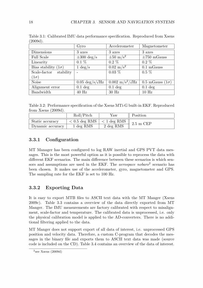
Table 3.1: Calibrated IMU data performance specification. Reproduced from Xsens(2009d).
Gyro Accelerometer MagnetometerDimensions 3 axes 3 axes 3 axesFull Scale ±300 deg/s ±50 m/s2 ±750 mGaussLinearity 0.1 % 0.2 % 0.2 %Bias stability (1σ) 1 deg/s 0.02 m/s2 0.1 mGaussScale-factor stability(1σ)
- 0.03 % 0.5 %
Noise 0.05 deg/s/√Hz 0.002 m/s2/√Hz 0.5 mGauss (1σ)Alignment error 0.1 deg 0.1 deg 0.1 degBandwidth 40 Hz 30 Hz 10 Hz
Table 3.2: Performance specification of the Xsens MTi-G built-in EKF. Reproducedfrom Xsens (2009d).
Roll/Pitch Yaw PositionStatic accuracy < 0.5 deg RMS < 1 deg RMS 2.5 m CEPDynamic accuracy 1 deg RMS 2 deg RMS
3.3.1 Configuration
MT Manager has been configured to log RAW inertial and GPS PVT data mes-sages. This is the most powerful option as it is possible to reprocess the data withdifferent EKF scenarios. The main difference between these scenarios is which sen-sors and assumptions are used in the EKF. The aerospace nobaro2 scenario hasbeen chosen. It makes use of the accelerometer, gyro, magnetometer and GPS.The sampling rate for the EKF is set to 100 Hz.
3.3.2 Exporting Data
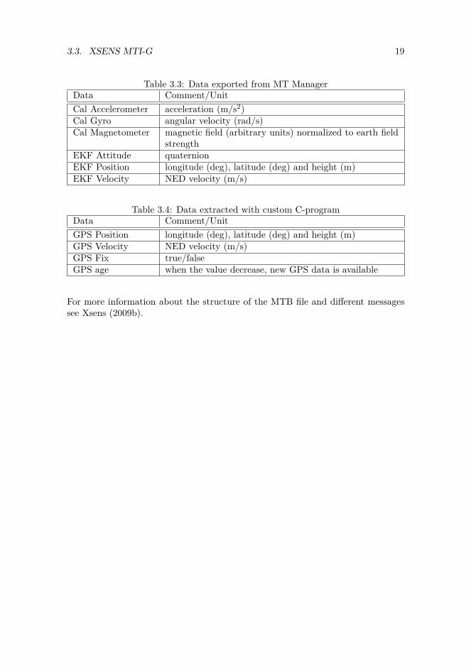
It is easy to export MTB files to ASCII text data with the MT Manger (Xsens2009c). Table 3.3 contains a overview of the data directly exported from MTManger. The IMU measurements are factory calibrated with respect to misalign-ment, scale-factor and temperature. The calibrated data is unprocessed, i.e. onlythe physical calibration model is applied to the AD-converters. There is no addi-tional filtering applied to the data.
MT Manger does not support export of all data of interest, i.e. unprocessed GPSposition and velocity data. Therefore, a custom C-program that decodes the mes-sages in the binary file and exports them to ASCII text data was made (sourcecode is included on the CD). Table 3.4 contains an overview of the data of interest.
2see Xsens (2009d)
3.3. XSENS MTI-G 19
Table 3.3: Data exported from MT ManagerData Comment/UnitCal Accelerometer acceleration (m/s2)Cal Gyro angular velocity (rad/s)Cal Magnetometer magnetic field (arbitrary units) normalized to earth field
strengthEKF Attitude quaternionEKF Position longitude (deg), latitude (deg) and height (m)EKF Velocity NED velocity (m/s)
Table 3.4: Data extracted with custom C-programData Comment/UnitGPS Position longitude (deg), latitude (deg) and height (m)GPS Velocity NED velocity (m/s)GPS Fix true/falseGPS age when the value decrease, new GPS data is available
For more information about the structure of the MTB file and different messagessee Xsens (2009b).

20 CHAPTER 3. SENSOR AND NAVIGATION SYSTEMS
Chapter 4
The q-method
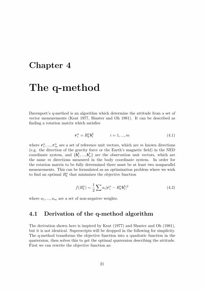
Davenport’s q-method is an algorithm which determine the attitude from a set ofvector measurements (Keat 1977, Shuster and Oh 1981). It can be described asfinding a rotation matrix which satisfies
rni = Rnb bbi i = 1, ...,m (4.1)
where rn1 , ..., rnm are a set of reference unit vectors, which are m known directions(e.g. the direction of the gravity force or the Earth’s magnetic field) in the NEDcoordinate system, and bb1, ..., b
bn are the observation unit vectors, which are
the same m directions measured in the body coordinate system. In order forthe rotation matrix to be fully determined there must be at least two nonparallelmeasurements. This can be formulated as an optimization problem where we wishto find an optimal Rnb that minimizes the objective function
f(Rnb ) = 12∑
ai|rni −Rnb bbi |2 (4.2)
where a1, ..., am are a set of non-negative weights.
4.1 Derivation of the q-method algorithm
The derivation shown here is inspired by Keat (1977) and Shuster and Oh (1981),but it is not identical. Superscripts will be dropped in the following for simplicity.The q-method transforms the objective function into a quadratic function in thequaternion, then solves this to get the optimal quaternion describing the attitude.First we can rewrite the objective function as:
21
22 CHAPTER 4. THE Q-METHOD
f(R) = 12∑
ai|ri −Rbi|2
= 12∑
ai[ri −Rbi]T [ri −Rbi]
= 12∑
ai(rTi ri − rTi Rbi − bTi R
Tri − biRTRbi)
= 12∑
ai(−2rTi Rbi)
= −∑
airTi Rbi (4.3)
where it is used that RRT = I. Terms independent of R has been canceled sincethey don’t affect the optimal R. The rotation matrix R can be expressed as afunction of the quaternions (2.5):
R(q) = I3×3 + 2ηε× + 2ε×ε×
= I3×3 + 2ηε× + 2εεT − 2εT εI3×3
= η2I3×3 + 2ηε× + 2εεT − εT εI3×3 (4.4)
where it is used that ε×ε× = εεT − εT εI3×3 and η2 + εT ε = 1. By inserting(4.4) into (4.3) the objective function can now be written as a function of thequaternions:
f(q) = −∑
airTi [η2I3×3 + 2ηε× + 2εεT − εT εI3×3]bi
= −∑
ai(η2rTi bi + 2ηrTi ε×bi + 2rTi εεT bi − εT εrTi bi)
= −∑
ai(η2rTi bi − η(r×i bi)T ε− ηεT (r×i bi) + ...
εTribTi ε+ εT birTi ε− εT εrTi bi)
= −η2σ + ηzT ε+ ηεTz − εTSε+ εT εσI3×3
=[η εT
] [ −σ zT
z −S + σI3×3
] [ηε
]= qTKq (4.5)
where the introduced variables are
4.1. DERIVATION OF THE Q-METHOD ALGORITHM 23
B =∑
airibTi (4.6)
σ = tr(B) =∑
airTi bi (4.7)
S = B +BT =∑
ai(ribTi + birTi ) (4.8)
z =∑
ai(r×i bi) (4.9)
K = KT =[−σ zT
z −S + σI3×3
](4.10)
The optimization problem has been reduced to
minq∈R4
f(q) = qTKq (4.11)
s.t.
qTq − 1 = 0 (4.12)
The Lagrangian function and it’s gradient for the problem is
L(q, λ) = qTKq − λ(qTq − 1) (4.13)OqL(q∗, λ∗) = 2Kq∗ − 2λ∗q∗ (4.14)
where the superscript ∗ denotes the optimal value and λ is the Lagrange multiplier.The first order optimality conditions often known as the KKT-conditions becomes(Nocedal and Wright 2006)
Kq∗ = λ∗q∗ (4.15)(q∗)Tq∗ = 1 (4.16)
Thus, the optimal point q∗ must be an eigenvector of K with λ∗ as the corre-sponding eigenvalue. Equation (4.15) is independent of the normalization of q∗and, therefore, (4.16) does not determine λ∗. However, by examining the objectivefunction in the optimal point
f(q∗) = (q∗)TKq∗ = λ∗(q∗)Tq∗ = λ∗ (4.17)
it’s seen that f will be minimized when λ∗ is the smallest eigenvalue of K. Hencethe optimal point q∗ is the eigenvector of K belonging to the smallest eigenvalueof K.
Kq∗ = λminq∗ (4.18)
The q-method algorithm can be summarized as follows:
24 CHAPTER 4. THE Q-METHOD
• Compute the symmetric 4×4 matrix K
• Compute the normalized eigenvector belonging to the smallest eigenvalue ofK
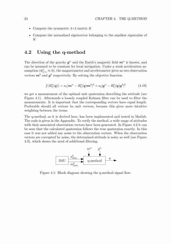
4.2 Using the q-method
The direction of the gravity gn and the Earth’s magnetic field mn is known, andcan be assumed to be constant for local navigation. Under a weak acceleration as-sumption (vnb/n ≈ 0), the magnetometer and accelerometer gives us two observationvectors mb and gb respectively. By solving the objective function
f(Rnb (q)) = a1|mn −Rnb (q)mb|2 + a2|gn −Rnb (q)gb|2 (4.19)
we get a measurement of the optimal unit quaternion describing the attitude (seeFigure 4.1). Afterwards a loosely coupled Kalman filter can be used to filter themeasurements. It is important that the corresponding vectors have equal length.Preferable should all vectors be unit vectors, because this gives more intuitiveweighting between the terms.
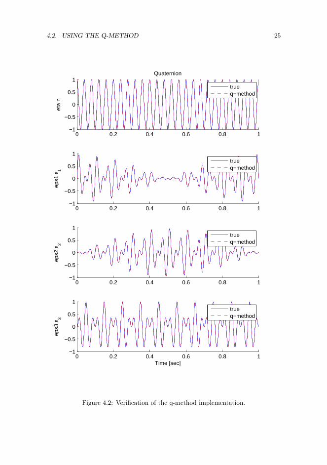
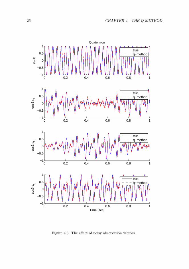
The q-method, as it is derived here, has been implemented and tested in Matlab.The code is given in the Appendix. To verify the method, a wide range of attitudeswith their associated observation vectors have been generated. In Figure 4.2 it canbe seen that the calculated quaternion follows the true quaternion exactly. In thiscase it was not added any noise to the observation vectors. When the observationvectors are corrupted by noise, the determined attitude is noisy as well (see Figure4.3), which shows the need of additional filtering.
abimu
IMU q-methodmb
imu
mn gn
q
Figure 4.1: Block diagram showing the q-method signal flow.
4.2. USING THE Q-METHOD 25
0 0.2 0.4 0.6 0.8 1−1
−0.5
0
0.5
1Quaternion
eta
η
trueq−method
0 0.2 0.4 0.6 0.8 1−1
−0.5
0
0.5
1
eps1
ε1
trueq−method
0 0.2 0.4 0.6 0.8 1−1
−0.5
0
0.5
1
eps2
ε2
trueq−method
0 0.2 0.4 0.6 0.8 1−1
−0.5
0
0.5
1
Time [sec]
eps3
ε3
trueq−method
Figure 4.2: Verification of the q-method implementation.
26 CHAPTER 4. THE Q-METHOD
0 0.2 0.4 0.6 0.8 1−1
−0.5
0
0.5
1Quaternion
eta
η
0 0.2 0.4 0.6 0.8 1−1
−0.5
0
0.5
1
eps1
ε1
0 0.2 0.4 0.6 0.8 1−1
−0.5
0
0.5
1
eps2
ε2
0 0.2 0.4 0.6 0.8 1−1
−0.5
0
0.5
1
Time [sec]
eps3
ε3
trueq−method
trueq−method
trueq−method
trueq−method
Figure 4.3: The effect of noisy observation vectors.
Chapter 5
Extended Kalman FilterDesign
The linear Kalman filter (KF) is simply an algorithm which produce optimal min-imum variance estimates, under the assumptions of Gaussian white noise and alinear observable system. However, as the inertial navigation equations are nonlin-ear the extended Kalman filter (EKF) will be used, which is the nonlinear variantof the usual KF. In the EKF the nonlinear system is linearized about the currentlybest estimate. It is commonly used in inertial navigation and many other fields.Stability and convergence of the EKF has been proven in Jouffroy and Fossen(2010), under the assumption of a lower and upper bounded covariance matrix.
In this chapter an extended Kalman filter for integration of GPS and IMU isderived. The goal is to estimate the position, velocity and attitude. The attitudewill be represented by the singularity free unit quaternion. Special care mustbe taken when designing a quaternion based extended Kalman filter (Vik n.d.).Because of the constraint on the quaternions, the covariance matrix P will besingular, and hence has an eigenvalue equal to zero. To maintain this singularity isvery difficult due to the accumulation of round-off errors in a numerical filter. Infact, this zero eigenvalue can even become negative and the filter becomes unstable.There exist several methods to deal with this singular covariance matrix. Most ofthem tries to reduce the dimension so that three parameters are used instead offour to describe the covariance of the four quaternions. The multiplicative extendedKalman filter (MEKF) handles this in an elegant way.
27
28 CHAPTER 5. EXTENDED KALMAN FILTER DESIGN
5.1 Discrete Multiplicative Extended Kalman Fil-ter
This section contains a brief introduction to the multiplicative extended Kalmanfilter (MEKF), a more in depth explanation can be found in Markley (2003). Theattitude is represented as the quaternion product
q = q ⊗ δq(δε) ⇔ Rnb (q) = Rnb(q)Rbb(δq) (5.1)
where q is some unit reference quaternion, representing the rotation from the ref-erence frame b to the NED frame n. Moreover
δq(δε) =[ √
1− δεT δεδε
](5.2)
is the attitude error, representing the rotation from the body frame b to thereference frame b. The MEKF computes an unconstrained estimate of the three-component δε, while using the four-component q to provide a globally non-singularattitude representation.
The filter proceeds in three steps: time propagation, measurement update, andreset. The discrete measurement update assigns a finite post-update value to δεk.In order to avoid the need to propagate two representations of the attitude, thereset operation moves the attitude information from δεk to qk, then δεk is reset tozero. Since true quaternion is not changed by this operation, (5.1) requires
qk−1 ⊗ δq(δεk) = qk ⊗ δq(0) = qk (5.3)
Given the discrete nonlinear system on the form
xk+1 = fk(xk,uk) + Γkwk (5.4)yk = hk(xk) + vk (5.5)
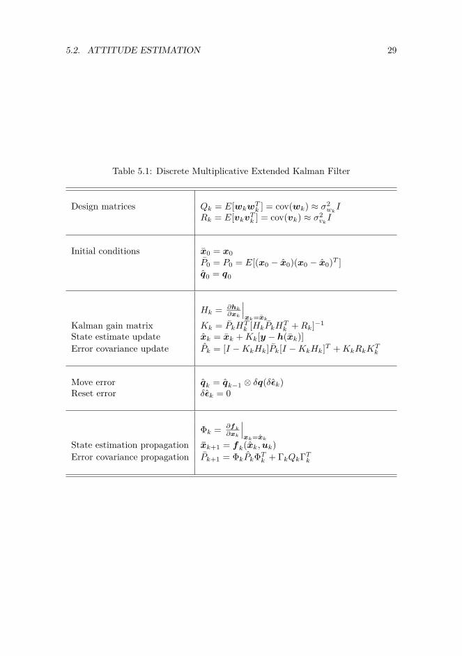
the discrete multiplicative extended Kalman filter algorithm can be summarized inTable 5.1.
5.2 Attitude Estimation
In this section we want to design a discrete multiplicative extended Kalman filterfor attitude estimation. By integrating attitude measurements and gyro measure-ments, we achieve two things:
5.2. ATTITUDE ESTIMATION 29
Table 5.1: Discrete Multiplicative Extended Kalman Filter
Design matrices Qk = E[wkwTk ] = cov(wk) ≈ σ2
wkI
Rk = E[vkvTk ] = cov(vk) ≈ σ2vkI
Initial conditions x0 = x0P0 = P0 = E[(x0 − x0)(x0 − x0)T ]q0 = q0
Hk = ∂hk
∂xk
∣∣∣xk=xk
Kalman gain matrix Kk = PkHTk [HkPkH
Tk +Rk]−1
State estimate update xk = xk +Kk[y − h(xk)]Error covariance update Pk = [I −KkHk]Pk[I −KkHk]T +KkRkK
Tk
Move error qk = qk−1 ⊗ δq(δεk)Reset error δεk = 0
Φk = ∂fk
∂xk
∣∣∣xk=xk
State estimation propagation xk+1 = fk(xk,uk)Error covariance propagation Pk+1 = ΦkPkΦTk + ΓkQkΓTk
30 CHAPTER 5. EXTENDED KALMAN FILTER DESIGN
• Low-pass filtering of the attitude measurements
• High-pass filtering of the gyro measurements
5.2.1 Assumptions
For this section we make the following assumptions:
• The vehicle has constant speed vnb/n = 0 and the accelerometer bias is zerobbacc = 0. These states are not observable without an additional position orvelocity measurement. Later these assumptions will be relaxed.
• The local magnetic disturbance is zero bbmag = 0. For a well calibrated mag-netometer, this is a reasonable assumption.
Consequently, we can write the accelerometer (3.8) and magnetometer (3.11) modelas
f bimu = −gb +wacc (5.6)mb
imu = mb +wmag (5.7)
5.2.2 Attitude Model
The time-derivative of δq is found by differentiating
δq = q−1 ⊗ q (5.8)
which is from the definition in (5.1). Considering that the resulting model will beused in a discrete-time filter, one can argue that because there is no time propaga-tion of q in the discrete filter, q will be constant between each sample. Hence wecan treat q as a constant when differentiating. This means that the change in theerror quaternion equals the change in the true quaternion. The following show thederivation of the time-derivative of δq:
5.2. ATTITUDE ESTIMATION 31
δq =[δηδε
]= q−1 ⊗ q
= 12 q−1 ⊗ q ⊗
[0
ωbb/n
]= 1
2δq ⊗[
0ωbb/n
]= 1
2Ω(ωbb/n)δq
= 12
[0 −(ωbb/n)T
ωbb/n −S(ωbb/n)
] [ √1− δεT δεδε
](5.9)
which gives the following vector part
δε = 12[ωbb/n
√1− δεT δε− S(ωbb/n)δε]
= 12 [I3×3
√1− δεT δε+ S(δε)]ωbb/n (5.10)
Because of the unit constraint on the error quaternion, it can be constructed fromthe vector part an any time. Thus it is sufficient to only estimate the vector partin the filter. In fact, this kind of model reduction is the goal in order to avoid thesingular covariance matrix.
For each iteration in the filter, the attitude information in the error quaternion willbe moved to q, in the reset operation. This ensures that the real part of the errorquaternion will be small. Consequently, the possible problems of a model reductiondiscussed in Vik (n.d.), Lefferts and Schuster (1982) are efficiently avoided.
Finally, the state variables in the filter are chosen to be x = [δε1, δε2, δε3, bp, bq, br]= [δε, bbgyro] and the input is u = ωbimu. Substituting (3.3) into (5.10), togetherwith (3.4) the attitude model can be written as
[δε
bb
gyro
]︸ ︷︷ ︸
x
=[ 1
2 [I3×3√
1− δεT δε+ S(δε)][ωbimu − bbgyro]
03×1
]︸ ︷︷ ︸
f(x,u)
+ I6×6︸︷︷︸Γ
[wgyrowbgyro
]︸ ︷︷ ︸
w
(5.11)
where w ∈ R6 is Gaussian white noise with zero mean and variance σ2w.
32 CHAPTER 5. EXTENDED KALMAN FILTER DESIGN
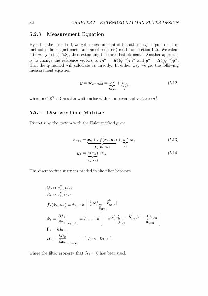
5.2.3 Measurement Equation
By using the q-method, we get a measurement of the attitude q. Input to the q-method is the magnetometer and accelerometer (recall from section 4.2). We calcu-late δε by using (5.8), then extracting the three last elements. Another approachis to change the reference vectors to mb = Rbn(q−1)mn and gb = Rbn(q−1)gn,then the q-method will calculate δε directly. In either way we get the followingmeasurement equation
y = δεqmetod = δε︸︷︷︸h(x)
+ wε︸︷︷︸v
(5.12)
where v ∈ R3 is Gaussian white noise with zero mean and variance σ2v .
5.2.4 Discrete-Time Matrices
Discretizing the system with the Euler method gives
xk+1 = xk + hf(xk,uk)︸ ︷︷ ︸fk(xk,uk)
+ hΓ︸︷︷︸Γk
wk (5.13)
yk = h(xk)︸ ︷︷ ︸hk(xk)
+vk (5.14)
The discrete-time matrices needed in the filter becomes
Qk ≈ σ2wkI6×6
Rk ≈ σ2vkI3×3
fk(xk,uk) = xk + h
[12 [ωbimu − b
b
gyro]03×1
]
Φk = ∂fk∂xk
∣∣∣∣xk=xk
= I6×6 + h
[− 1
2S(ωbimu − bb
gyro) − 12I3×3
03×3 03×3
]Γk = hI6×6
Hk = ∂hk∂xk
∣∣∣∣xk=xk
=[I3×3 03×3
]where the filter property that δεk = 0 has been used.
5.2. ATTITUDE ESTIMATION 33
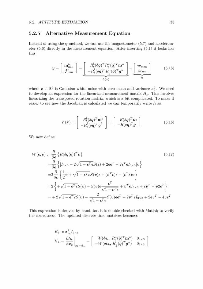
5.2.5 Alternative Measurement Equation
Instead of using the q-method, we can use the magnetometer (5.7) and accelerom-eter (5.6) directly in the measurement equation. After inserting (5.1) it looks likethis
y =[
mbimu
f bimu
]=[
Rbb(δq)TRnb(q)Tmn
−Rbb(δq)TRnb(q)Tgn
]︸ ︷︷ ︸
h(x)
+[wmagwacc
]︸ ︷︷ ︸
v
(5.15)
where v ∈ R6 is Gaussian white noise with zero mean and variance σ2v . We need
to develop an expression for the linearized measurement matrix Hk. This involveslinearizing the transposed rotation matrix, which is a bit complicated. To make iteasier to see how the Jacobian is calculated we can temporarily write h as
h(x) =[
Rbb(δq)Tmb
−Rbb(δq)Tgb
]=[
R(δq)Tm−R(δq)Tg
](5.16)
We now define
W (ε,v) := ∂
∂ε
R(δq(ε))Tv
(5.17)
= ∂
∂ε
[I3×3 − 2
√1− εT εS(ε) + 2εεT − 2εT εI3×3]v
=2 ∂
∂ε
12v +
√1− εT εS(v)ε+ (vT ε)ε− (εT ε)v
=2
+√
1− εT εS(v)− S(v)ε εT√1− εT ε
+ vT εI3×3 + εvT − v2εT
= + 2√
1− εT εS(v)− 2√1− εT ε
S(v)εεT + 2vT εI3×3 + 2εvT − 4vεT
This expression is derived by hand, but it is double checked with Matlab to verifythe correctness. The updated discrete-time matrices becomes
Rk ≈ σ2vkI6×6
Hk = ∂hk∂xk
∣∣∣∣xk=xk
=[
W (δεk, Rnb (q)Tmn) 03×3−W (δεk, Rnb (q)Tgn) 03×3
]
34 CHAPTER 5. EXTENDED KALMAN FILTER DESIGN
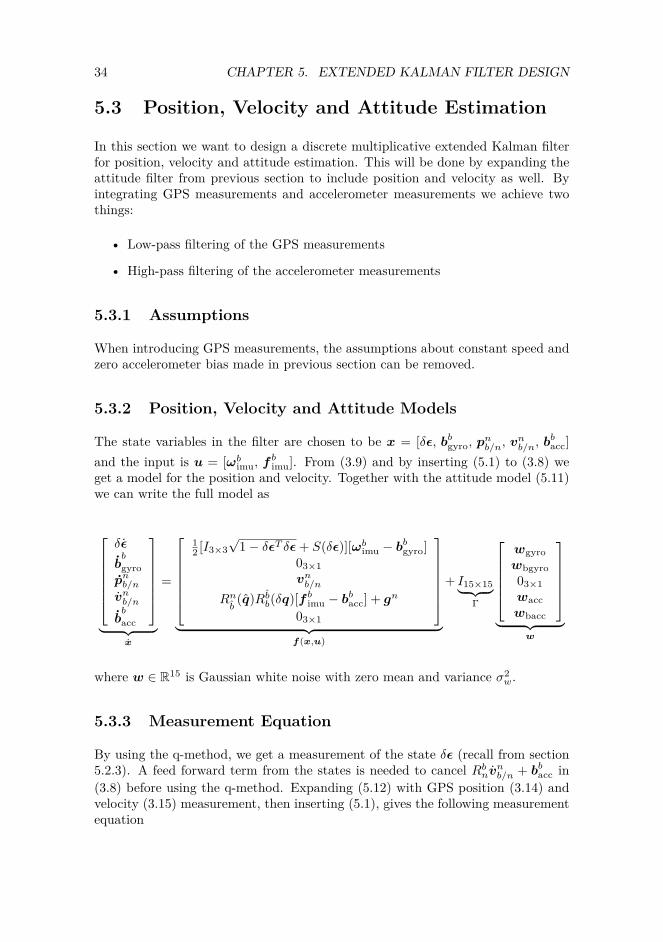
5.3 Position, Velocity and Attitude Estimation
In this section we want to design a discrete multiplicative extended Kalman filterfor position, velocity and attitude estimation. This will be done by expanding theattitude filter from previous section to include position and velocity as well. Byintegrating GPS measurements and accelerometer measurements we achieve twothings:
• Low-pass filtering of the GPS measurements
• High-pass filtering of the accelerometer measurements
5.3.1 Assumptions
When introducing GPS measurements, the assumptions about constant speed andzero accelerometer bias made in previous section can be removed.
5.3.2 Position, Velocity and Attitude Models
The state variables in the filter are chosen to be x = [δε, bbgyro, pnb/n, v
nb/n, b
bacc]
and the input is u = [ωbimu, fbimu]. From (3.9) and by inserting (5.1) to (3.8) we
get a model for the position and velocity. Together with the attitude model (5.11)we can write the full model as
δε
bb
gyropnb/nvnb/n
bb
acc
︸ ︷︷ ︸
x
=
12 [I3×3
√1− δεT δε+ S(δε)][ωbimu − b
bgyro]
03×1vnb/n
Rnb(q)Rbb(δq)[f bimu − b
bacc] + gn
03×1
︸ ︷︷ ︸
f(x,u)
+ I15×15︸ ︷︷ ︸Γ
wgyrowbgyro03×1waccwbacc
︸ ︷︷ ︸
w
where w ∈ R15 is Gaussian white noise with zero mean and variance σ2w.
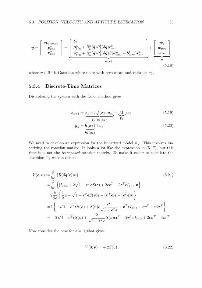
5.3.3 Measurement Equation
By using the q-method, we get a measurement of the state δε (recall from section5.2.3). A feed forward term from the states is needed to cancel Rbnvnb/n + bbacc in(3.8) before using the q-method. Expanding (5.12) with GPS position (3.14) andvelocity (3.15) measurement, then inserting (5.1), gives the following measurementequation
5.3. POSITION, VELOCITY AND ATTITUDE ESTIMATION 35
y =
δεqmetodpngpsvngps
=
δε
pnb/n +Rnb(q)Rbb(δq)rbant
vnb/n +Rnb(q)Rbb(δq)S(ωbimu − b
bgyro)rbant
︸ ︷︷ ︸
h(x)
+
wε
wposwvel
︸ ︷︷ ︸
v
(5.18)
where v ∈ R9 is Gaussian white noise with zero mean and variance σ2v .
5.3.4 Discrete-Time Matrices
Discretizing the system with the Euler method gives
xk+1 = xk + hf(xk,uk)︸ ︷︷ ︸fk(xk,uk)
+ hΓ︸︷︷︸Γk
wk (5.19)
yk = h(xk)︸ ︷︷ ︸hk(xk)
+vk (5.20)
We need to develop an expression for the linearized model Φk. This involves lin-earizing the rotation matrix. It looks a lot like the expression in (5.17), but thistime it is not the transposed rotation matrix. To make it easier to calculate theJacobian Φk we can define
V (ε,v) := ∂
∂εR(δq(ε))v (5.21)
= ∂
∂ε
[I3×3 + 2
√1− εT εS(ε) + 2εεT − 2εT εI3×3]v
=2 ∂
∂ε
12v −
√1− εT εS(v)ε+ (vT ε)ε− (εT ε)v
=2−√
1− εT εS(v) + S(v)ε εT√1− εT ε
+ vT εI3×3 + εvT − v2εT
=− 2√
1− εT εS(v) + 2√1− εT ε
S(v)εεT + 2vT εI3×3 + 2εvT − 4vεT
Now consider the case for ε = 0, that gives
V (0,v) =− 2S(v) (5.22)
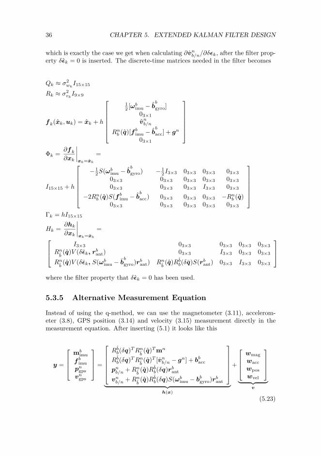
36 CHAPTER 5. EXTENDED KALMAN FILTER DESIGN
which is exactly the case we get when calculating ∂vnb/n/∂δεk, after the filter prop-erty δεk = 0 is inserted. The discrete-time matrices needed in the filter becomes
Qk ≈ σ2wkI15×15
Rk ≈ σ2vkI9×9
fk(xk,uk) = xk + h
12 [ωbimu − b
b
gyro]03×1vnb/n
Rnb (q)[f bimu − bb
acc] + gn03×1
Φk = ∂fk
∂xk
∣∣∣∣xk=xk
=
I15×15 + h
− 1
2S(ωbimu − bb
gyro) − 12I3×3 03×3 03×3 03×3
03×3 03×3 03×3 03×3 03×303×3 03×3 03×3 I3×3 03×3
−2Rnb (q)S(f bimu − bb
acc) 03×3 03×3 03×3 −Rnb (q)03×3 03×3 03×3 03×3 03×3
Γk = hI15×15
Hk = ∂hk∂xk
∣∣∣∣xk=xk
= I3×3 03×3 03×3 03×3 03×3Rnb(q)V (δεk, rbant) 03×3 I3×3 03×3 03×3
Rnb(q)V (δεk, S(ωbimu − b
b
gyro)rbant) Rnb(q)Rbb(δq)S(rbant) 03×3 I3×3 03×3
where the filter property that δεk = 0 has been used.
5.3.5 Alternative Measurement Equation
Instead of using the q-method, we can use the magnetometer (3.11), accelerom-eter (3.8), GPS position (3.14) and velocity (3.15) measurement directly in themeasurement equation. After inserting (5.1) it looks like this
y =
mb
imuf bimupngpsvngps
=
Rbb(δq)TRn
b(q)Tmn
Rbb(δq)TRnb(q)T [vnb/n − gn] + bbacc
pnb/n +Rnb(q)Rbb(δq)rbant
vnb/n +Rnb(q)Rbb(δq)S(ωbimu − b
bgyro)rbant
︸ ︷︷ ︸
h(x)
+
wmagwaccwposwvel
︸ ︷︷ ︸
v
(5.23)

5.3. POSITION, VELOCITY AND ATTITUDE ESTIMATION 37
where v ∈ R12 is Gaussian white noise with zero mean and variance σ2v . The
updated discrete-time matrices becomes
Rk ≈ σ2vkI12×12
Hk = ∂hk∂xk
∣∣∣∣xk=xk
=W (δεk, Rnb (q)Tmn) 03×3 03×3 03×3 03×3−W (δεk, Rnb (q)Tgn) 03×3 03×3 03×3 I3×3Rnb(q)V (δεk, rbant) 03×3 I3×3 03×3 03×3
Rnb(q)V (δεk, S(ωbimu − b
b
gyro)rbant) Rnb(q)Rbb(δq)S(rbant) 03×3 I3×3 03×3

38 CHAPTER 5. EXTENDED KALMAN FILTER DESIGN
Chapter 6
Nonlinear Observer Design
Tuning of the Kalman filter is a difficult and time consuming task. The elementsin the measurement covariance matrix R can often be found in the data sheet forthe sensors, but the elements in the process covariance matrix Q is often difficult torelate to physical quantities. Also the Riccati equation is computational extensive.This is some of the reasons why there has been an increasing interest for nonlinearobserver design the last decades (Fossen 2011).
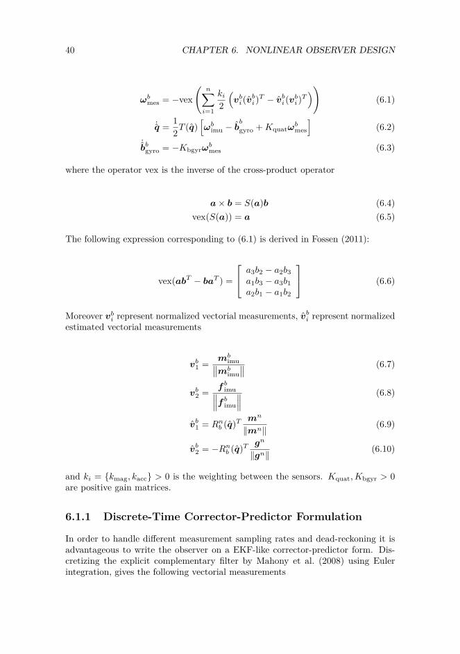
In this chapter a nonlinear observer for integration of IMU and GPS is derived. Theobserver is made of a combination of two nonlinear algorithms recently proposedby Hua (2010) and Mahony et al. (2008). Later the performance of the nonlinearobserver will be compared with the extended Kalman filter to see whether it hascompetitive results.
6.1 Attitude Observer
Mahony et al. (2008) has proposed an observer, termed the explicit complementaryfilter, that provides attitude estimates as well as gyro bias estimates. Vectorialmeasurements, such as gravitational and magnetic field directions, are used di-rectly without algebraic reconstruction of the attitude. It remains well conditionedin the case where only a single vector direction is measured. The observer is wellsuited for implementation on embedded hardware platforms. Local exponentialand almost global stability of the observer error dynamics have been shown withLyapunov analysis, for 2 or more independent inertial directions. The accelerom-eter measurement is approximated to be a gravity measurement (vnb/n ≈ 0). Thequaternion representation of the explicit complementary filter by Mahony et al.(2008) is:
39
40 CHAPTER 6. NONLINEAR OBSERVER DESIGN
ωbmes = −vex(
n∑i=1
ki2
(vbi (v
bi )T − v
bi (vbi )T
))(6.1)
˙q = 12T (q)
[ωbimu − b
b
gyro +Kquatωbmes
](6.2)
˙bbgyro = −Kbgyrω
bmes (6.3)
where the operator vex is the inverse of the cross-product operator
a× b = S(a)b (6.4)vex(S(a)) = a (6.5)
The following expression corresponding to (6.1) is derived in Fossen (2011):
vex(abT − baT ) =
a3b2 − a2b3a1b3 − a3b1a2b1 − a1b2
(6.6)
Moreover vbi represent normalized vectorial measurements, vbi represent normalizedestimated vectorial measurements
vb1 = mbimu∥∥mbimu∥∥ (6.7)
vb2 = f bimu∥∥∥f bimu
∥∥∥ (6.8)
vb1 = Rnb (q)T mn
‖mn‖(6.9)
vb2 = −Rnb (q)T gn
‖gn‖(6.10)
and ki = kmag, kacc > 0 is the weighting between the sensors. Kquat,Kbgyr > 0are positive gain matrices.
6.1.1 Discrete-Time Corrector-Predictor Formulation
In order to handle different measurement sampling rates and dead-reckoning it isadvantageous to write the observer on a EKF-like corrector-predictor form. Dis-cretizing the explicit complementary filter by Mahony et al. (2008) using Eulerintegration, gives the following vectorial measurements
6.2. POSITION, VELOCITY AND ATTITUDE OBSERVER 41
vb1 = mbimu(k)∥∥mbimu(k)
∥∥ (6.11)
vb2 = f bimu(k)∥∥∥f bimu(k)∥∥∥ (6.12)
vb1 = Rnb (q(k))T mn
‖mn‖(6.13)
vb2 = −Rnb (q(k))T gn
‖gn‖(6.14)
and the corrector becomes
ωbmes = −vex(
n∑i=1
ki2(vbi (vbi )T − vbi (vbi )T
))(6.15)
q(k) = q(k) + h · 12T (q(k))Kquatω
bmes (6.16)
bb
gyro(k) = bb
gyro(k)− h ·Kbgyrωbmes (6.17)
and the predictor becomes
q(k + 1) = q(k) + h · 12T (q(k))
[ωbimu(k)− b
b
gyro(k)]
(6.18)
bb
gyro(k + 1) = bb
gyro(k) (6.19)
6.2 Position, Velocity and Attitude Observer
Hua (2010) has recently proposed an advanced observer, that provides estimatesof attitude and velocity. The observer makes use of accelerometer, magnetometerand linear velocity measurements, which makes it better adapted for vehicles sub-jected to important linear accelerations. Stability analysis results state semi-globalconvergence. The observer proposed by Hua (2010) is
42 CHAPTER 6. NONLINEAR OBSERVER DESIGN
˙vnb/n = Qf bimu + gn + kvel(vngps − vnb/n) (6.20)
Q = QS(ωbimu)− ρQ+ kQ(vngps − vnb/n)(f bimu)T (6.21)
ρ = knormmax(0, ‖Q‖ −√
3) (6.22)˙Rnb = Rnb S(ωbimu + σ) (6.23)σ = kmagm
bimu × (Rnb )Tmn + kaccf
bimu × (Rnb )T (Qf bimu + kvel(vngps − v
nb/n))(6.24)
where kvel, kmag, kacc, kQ, knorm is some positive constant gains, and Q ∈ R3×3
is a virtual matrix that allows an estimation of the specific acceleration in theinertial frame n. It is not a rotation matrix but still such that Qf bimu −Rnb f
bimu
tends to zero. ‖Q‖ is the Frobenius norm, i.e. ‖Q‖ =√
tr(QTQ). One can viewQf bimu + kvel(vngps − v
nb/n) as an estimate of fn.
The observer of Hua (2010) does not provide estimates of the gyro bias. But as theobserver of Mahony et al. (2008) has gyro bias estimation, the attitude part, (6.23)and (6.24), can be removed and replaced with the attitude observer of Mahonyet al. (2008). This will be a combination of the advantage of the linear accelerationestimation from Hua together with gyro bias estimation from Mahony. It is straightforward to modify the observer to include position as well by adding
˙pnb/n = vnb/n + kpos(pngps − pnb/n) (6.25)
where kpos is a positive gain.
6.2.1 Discrete-Time Corrector-Predictor Formulation
In the following the discrete-time corrector-predictor formulation for the combinedHua (2010) and Mahony et al. (2008) observer will be derived using Euler inte-gration. As the specific acceleration is estimated the vectorial measurements willbe
6.2. POSITION, VELOCITY AND ATTITUDE OBSERVER 43
vb1 = mbimu(k)∥∥mbimu(k)
∥∥ (6.26)
vb2 = f bimu(k)∥∥∥f bimu(k)∥∥∥ (6.27)
vb1 = Rnb (q(k))T mn
‖mn‖(6.28)
vb2 = Rnb (q(k))TQ(k)f bimu(k) + kvel(vngps(k)− vnb/n(k))∥∥∥Q(k)f bimu(k) + kvel(vngps(k)− vnb/n(k))
∥∥∥ (6.29)
and the corrector becomes
pnb/n(k) = pnb/n(k) + h · kpos(pngps(k)− pnb/n(k)) (6.30)vnb/n(k) = vnb/n(k) + h · kvel(vngps(k)− vnb/n(k)) (6.31)
Q(k) = Q(k) + h · kQ(vngps(k)− vnb/n(k))(f bimu(k))T (6.32)
together with (6.15), (6.16) and (6.17). The predictor becomes
pnb/n(k + 1) = pnb/n(k) + h · vnb/n(k) (6.33)
vnb/n(k + 1) = vnb/n(k) + h · (Q(k)f bimu(k) + gn) (6.34)
Q(k + 1) = Q(k) + h · Q(k)S(ωbimu(k)) (6.35)
together with (6.18) and (6.19). The “normalization” term ρQ has been removed.It should be replaced by the discrete variant
Q(k) = Q(k)‖Q(k)‖
√3 (6.36)
and used after any calculations on Q.

44 CHAPTER 6. NONLINEAR OBSERVER DESIGN
Chapter 7
Simulator
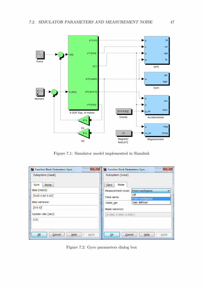
It is convenient to have a simulator that can generate IMU and GPS measure-ments during development, testing and verification of the nonlinear observers. Forinstance faults can be simulated to test the observer error handling. This chaptercontains a unmanned aerial vehicle (UAV) model as well as sensor and navigationsystem models. The simulator has been implemented in Simulink.
7.1 Simulator Model
This section contains the equations needed to implement the simulator that gener-ates IMU and GPS measurements. The 6 DOF kinematic equations are given byFossen (2011):
pnb/n = Rnb (q)vbb/n (7.1)
q = 12T (q)ωbb/n + γ
2 (1− qTq)q (7.2)
where a feedback term has been added to (7.2). The feedback term drives thequaternion to a unit quaternion in order to compensate for numerical round oferrors. The normalization gain can be set to γ = 100. The 6 DOF equations ofmotion are given by Fossen (2011):
m[vbb/n + S(ωbb/n)vbb/n] +D1vbb/n = f b (7.3)
Ibωbb/n + S(ωbb/n)Ibωbb/n +D2ω
bb/n = mb (7.4)
45
46 CHAPTER 7. SIMULATOR
where f b and mb is forces and moments respectively, D1, D2 are linear dampingmatrices and Ib is the inertia matrix. The center of origin (CO) for the body framehas been chosen such that it coincides with the center of gravity (CG) . The gyromeasurement is modeled according to (3.3) and (3.4)
ygyro = ωbb/n + bbgyro +wgyro (7.5)
bb
gyro = wbgyro (7.6)
The accelerometer model is given by (3.7) and (3.9)
yacc = abb/n −Rnb (q)Tgn + bbacc +wacc, abb/n = vbb/n + S(ωbb/n)vbb/n (7.7)
bb
acc = wbacc (7.8)
The magnetometer model is given by (3.11)
ymag = Rnb (q)T mn
‖mn‖+ bbmag +wmag (7.9)
The GPS model is given by (3.14) and (3.15)
ypos = pnb/n +Rnb (q)rbant +wpos (7.10)
yvel = vnb/n +Rnb (q)S(ωbb/n)rbant +wvel (7.11)
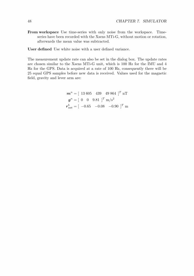
7.2 Simulator Parameters and Measurement Noise
The simulator parameters can be set in the various parameter dialog boxes. SeeFigure 7.2 for an example of the gyro parameters dialog box. For simplicity thefollowing parameters are used for the vehicle model
m = 1, Ib = I3×3, D1 = I3×3, D2 = I3×3 (7.12)
The simulator has three different options for the measurement noise wgyro, wacc,wmag, wpos and wvel (see Figure 7.2):
Off The measurement noise is off, i.e. w = 0
7.2. SIMULATOR PARAMETERS AND MEASUREMENT NOISE 47
Moment
Magnetometer
q
m_ref
mag
bmag
Magneticfield [nT]
-C-
Gyro
w
gyr
bgyr
Gravity
[0 0 9.81]'
GPS
p
v
q
w
llh
vel
age
fixForce
D2
K*u
D1
K*uAccelerometer
a
q
g_ref
acc
bacc6 DOF Eqs. of motion
f [N]
m [Nm]
p^n [m]
v^n [m/s]
q [-]
w^b [rad/s]
a^b [m/s^2]
v^b [m/s]
Figure 7.1: Simulator model implemented in Simulink
Figure 7.2: Gyro parameters dialog box
48 CHAPTER 7. SIMULATOR
From workspace Use time-series with only noise from the workspace. Time-series have been recorded with the Xsens MTi-G, without motion or rotation,afterwards the mean value was subtracted.
User defined Use white noise with a user defined variance.
The measurement update rate can also be set in the dialog box. The update ratesare chosen similar to the Xsens MTi-G unit, which is 100 Hz for the IMU and 4Hz for the GPS. Data is acquired at a rate of 100 Hz, consequently there will be25 equal GPS samples before new data is received. Values used for the magneticfield, gravity and lever arm are:
mn = [ 13 605 439 49 864 ]T nTgn = [ 0 0 9.81 ]T m/s2
rbant = [ −0.65 −0.08 −0.90 ]T m
Chapter 8
Implementation
The nonlinear observers developed in this thesis have been implemented in Matlab.The Workspace in Matlab have been used to interface the measurement time-series.This makes it easy to switch between simulated data and experimental data withoutdoing any changes. When it comes to implementation, there are some things thatneed to be addressed. This chapter highlights some implementation considerationsas well as error handling for the nonlinear observers in this thesis.
8.1 Numerical Properties of Different Attitude Rep-resentations
The attitude can be represented in several ways, i.e. quaternion or rotation matrix.They have different numerical properties when dicretized. Discretizing the differ-ential equation for the quaternion and the rotation matrix using the Euler methodgives
q(k + 1) = q(k) + h · 12T (q(k))ωbb/n(k) (8.1)
Rnb (k + 1) = Rnb (k) + h · Rnb (k)S(ωbb/n(k)) (8.2)
Numerical round-off errors will cause a violation of the unit constraint on thequaternion. To ensure that the constraint is satisfied the following normalizationprocedure can be used
q(k + 1) = q(k + 1)‖q(k + 1)‖ (8.3)
49
50 CHAPTER 8. IMPLEMENTATION
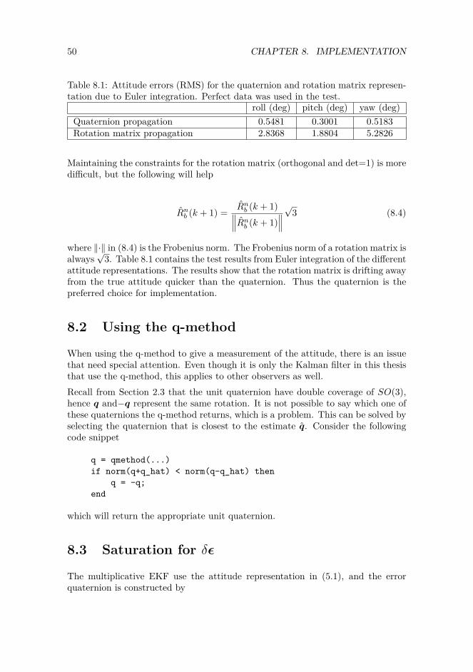
Table 8.1: Attitude errors (RMS) for the quaternion and rotation matrix represen-tation due to Euler integration. Perfect data was used in the test.
roll (deg) pitch (deg) yaw (deg)Quaternion propagation 0.5481 0.3001 0.5183Rotation matrix propagation 2.8368 1.8804 5.2826
Maintaining the constraints for the rotation matrix (orthogonal and det=1) is moredifficult, but the following will help
Rnb (k + 1) = Rnb (k + 1)∥∥∥Rnb (k + 1)∥∥∥√
3 (8.4)
where ‖·‖ in (8.4) is the Frobenius norm. The Frobenius norm of a rotation matrix isalways
√3. Table 8.1 contains the test results from Euler integration of the different
attitude representations. The results show that the rotation matrix is drifting awayfrom the true attitude quicker than the quaternion. Thus the quaternion is thepreferred choice for implementation.
8.2 Using the q-method
When using the q-method to give a measurement of the attitude, there is an issuethat need special attention. Even though it is only the Kalman filter in this thesisthat use the q-method, this applies to other observers as well.Recall from Section 2.3 that the unit quaternion have double coverage of SO(3),hence q and−q represent the same rotation. It is not possible to say which one ofthese quaternions the q-method returns, which is a problem. This can be solved byselecting the quaternion that is closest to the estimate q. Consider the followingcode snippet
q = qmethod(...)if norm(q+q_hat) < norm(q-q_hat) then
q = -q;end
which will return the appropriate unit quaternion.
8.3 Saturation for δε
The multiplicative EKF use the attitude representation in (5.1), and the errorquaternion is constructed by
8.4. DEAD-RECKONING 51
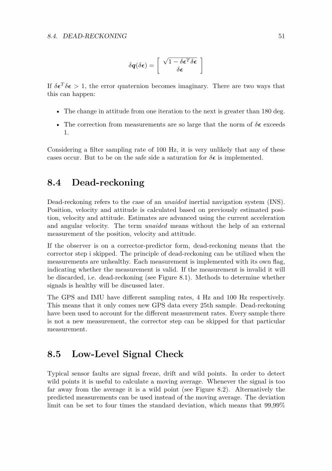
δq(δε) =[ √
1− δεT δεδε
]If δεT δε > 1, the error quaternion becomes imaginary. There are two ways thatthis can happen:
• The change in attitude from one iteration to the next is greater than 180 deg.
• The correction from measurements are so large that the norm of δε exceeds1.
Considering a filter sampling rate of 100 Hz, it is very unlikely that any of thesecases occur. But to be on the safe side a saturation for δε is implemented.
8.4 Dead-reckoning
Dead-reckoning refers to the case of an unaided inertial navigation system (INS).Position, velocity and attitude is calculated based on previously estimated posi-tion, velocity and attitude. Estimates are advanced using the current accelerationand angular velocity. The term unaided means without the help of an externalmeasurement of the position, velocity and attitude.
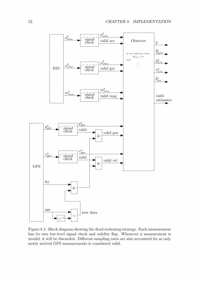
If the observer is on a corrector-predictor form, dead-reckoning means that thecorrector step i skipped. The principle of dead-reckoning can be utilized when themeasurements are unhealthy. Each measurement is implemented with its own flag,indicating whether the measurement is valid. If the measurement is invalid it willbe discarded, i.e. dead-reckoning (see Figure 8.1). Methods to determine whethersignals is healthy will be discussed later.
The GPS and IMU have different sampling rates, 4 Hz and 100 Hz respectively.This means that it only comes new GPS data every 25th sample. Dead-reckoninghave been used to account for the different measurement rates. Every sample thereis not a new measurement, the corrector step can be skipped for that particularmeasurement.
8.5 Low-Level Signal Check
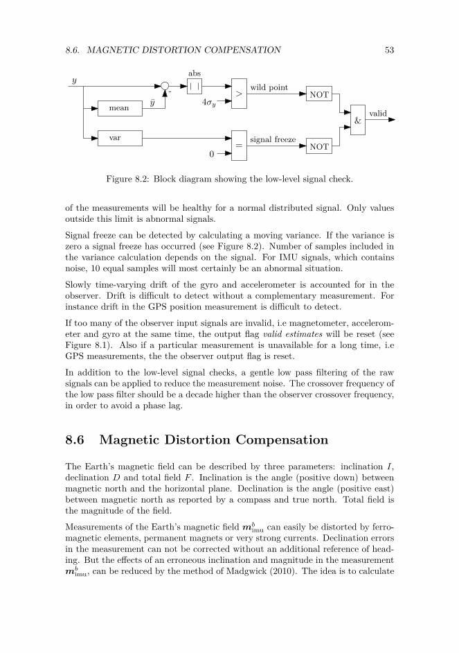
Typical sensor faults are signal freeze, drift and wild points. In order to detectwild points it is useful to calculate a moving average. Whenever the signal is toofar away from the average it is a wild point (see Figure 8.2). Alternatively thepredicted measurements can be used instead of the moving average. The deviationlimit can be set to four times the standard deviation, which means that 99,99%
52 CHAPTER 8. IMPLEMENTATION
<z−1
vngps
fix
agenew data
validvalid vel
&
pngpsvalid
valid pos
GPS
valid acc
abimu
valid gyr
ωbimu
valid mag
mbimu
abimu
ωbimu
mbimu
IMU
vngps
pngps
if not valid acc then
Kacc = 0
Observer
...
end
q
bbgyro
pnb/n
vnb/n
bbacc
&
&
signalcheck
signalcheck
signalcheck
signalcheck
signalcheck
validestimates
Figure 8.1: Block diagram showing the dead-reckoning strategy. Each measurementhas its own low-level signal check and validity flag. Whenever a measurement isinvalid, it will be discarded. Different sampling rates are also accounted for as onlynewly arrived GPS measurements is considered valid.
8.6. MAGNETIC DISTORTION COMPENSATION 53
mean
var
-y
yabs
>4σy
=0
wild point
signal freeze
NOT
NOT
&valid
Figure 8.2: Block diagram showing the low-level signal check.
of the measurements will be healthy for a normal distributed signal. Only valuesoutside this limit is abnormal signals.
Signal freeze can be detected by calculating a moving variance. If the variance iszero a signal freeze has occurred (see Figure 8.2). Number of samples included inthe variance calculation depends on the signal. For IMU signals, which containsnoise, 10 equal samples will most certainly be an abnormal situation.
Slowly time-varying drift of the gyro and accelerometer is accounted for in theobserver. Drift is difficult to detect without a complementary measurement. Forinstance drift in the GPS position measurement is difficult to detect.
If too many of the observer input signals are invalid, i.e magnetometer, accelerom-eter and gyro at the same time, the output flag valid estimates will be reset (seeFigure 8.1). Also if a particular measurement is unavailable for a long time, i.eGPS measurements, the the observer output flag is reset.
In addition to the low-level signal checks, a gentle low pass filtering of the rawsignals can be applied to reduce the measurement noise. The crossover frequency ofthe low pass filter should be a decade higher than the observer crossover frequency,in order to avoid a phase lag.
8.6 Magnetic Distortion Compensation
The Earth’s magnetic field can be described by three parameters: inclination I,declination D and total field F . Inclination is the angle (positive down) betweenmagnetic north and the horizontal plane. Declination is the angle (positive east)between magnetic north as reported by a compass and true north. Total field isthe magnitude of the field.
Measurements of the Earth’s magnetic field mbimu can easily be distorted by ferro-
magnetic elements, permanent magnets or very strong currents. Declination errorsin the measurement can not be corrected without an additional reference of head-ing. But the effects of an erroneous inclination and magnitude in the measurementmb
imu, can be reduced by the method of Madgwick (2010). The idea is to calculate
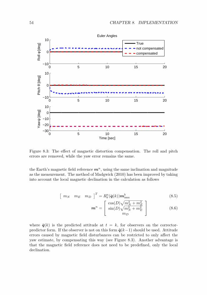
54 CHAPTER 8. IMPLEMENTATION
0 5 10 15 20−10
0
10Euler Angles
Rol
l φ [d
eg]
0 5 10 15 20−10
0
10
Pitc
h θ
[deg
]
Truenot compensatedcompensated
0 5 10 15 20−30
−20
−10
0
10
Yaw
ψ [d
eg]
Time [sec]
Figure 8.3: The effect of magnetic distortion compensation. The roll and pitcherrors are removed, while the yaw error remains the same.
the Earth’s magnetic field referencemn, using the same inclination and magnitudeas the measurement. The method of Madgwick (2010) has been improved by takinginto account the local magnetic declination in the calculation as follows
[mN mE mD
]T = Rnb (q(k))mbimu (8.5)
mn =
cos(D)√m2N +m2
E
sin(D)√m2N +m2
E
mD
(8.6)
where q(k) is the predicted attitude at t = k, for observers on the corrector-predictor form. If the observer is not on this form q(k−1) should be used. Attitudeerrors caused by magnetic field disturbances can be restricted to only affect theyaw estimate, by compensating this way (see Figure 8.3). Another advantage isthat the magnetic field reference does not need to be predefined, only the localdeclination.
Chapter 9
Simulation Results
This chapter contains a case study of the nonlinear observers developed in this the-sis, demonstrating how different disturbances affects the estimates. The simulatordeveloped in Chapter 7 have been used to generate IMU and GPS measurements.Test results of the performance are given as Root Mean Square (RMS) errors, whichis calculated by the following formula
RMS =
√√√√ 1N
N∑i=1
(x(i)− xtrue(i))2
where N is the number of samples in the time-serie, and x represent roll, pitch andso on. The first 40 seconds have been omitted in the RMS calculation to removemost of the transient part. Tests have been carried out for the following observers:MEKF is the multiplicative extended Kalman filter including attitude, positionand velocity estimates. The filter was derived with two different measurementequations; one using the q-method and the other using vectorial measurements.The vectorial measurement equation is used. The following Kalman filter tuningmatrices have been used
Qk = diag( 5e-71×2 5e-6 5e-81×2 1e-7 1e-41×3 1e-41×3 1e-71×3 )Rk = diag( 2e-51×3 2e-31×3 101×3 1e-41×3 )P0 = diag( 1e-51×3 1e-91×3 01×3 1e-41×3 1e-81×3 )
HuaMahony is the nonlinear observer combination of Hua (2010) and Mahonyet al. (2008) including attitude, position and velocity estimates. The discrete-time corrector-predictor formulation of HuaMahony has been implemented. Thefollowing observer gains have been used
55
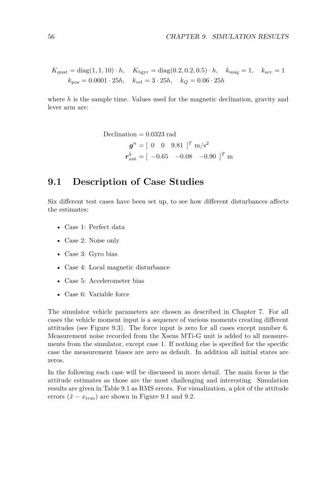
56 CHAPTER 9. SIMULATION RESULTS
Kquat = diag(1, 1, 10) · h, Kbgyr = diag(0.2, 0.2, 0.5) · h, kmag = 1, kacc = 1kpos = 0.0001 · 25h, kvel = 3 · 25h, kQ = 0.06 · 25h
where h is the sample time. Values used for the magnetic declination, gravity andlever arm are:
Declination = 0.0323 radgn = [ 0 0 9.81 ]T m/s2
rbant = [ −0.65 −0.08 −0.90 ]T m
9.1 Description of Case Studies
Six different test cases have been set up, to see how different disturbances affectsthe estimates:
• Case 1: Perfect data
• Case 2: Noise only
• Case 3: Gyro bias
• Case 4: Local magnetic disturbance
• Case 5: Accelerometer bias
• Case 6: Variable force
The simulator vehicle parameters are chosen as described in Chapter 7. For allcases the vehicle moment input is a sequence of various moments creating differentattitudes (see Figure 9.3). The force input is zero for all cases except number 6.Measurement noise recorded from the Xsens MTi-G unit is added to all measure-ments from the simulator, except case 1. If nothing else is specified for the specificcase the measurement biases are zero as default. In addition all initial states arezeros.
In the following each case will be discussed in more detail. The main focus is theattitude estimates as those are the most challenging and interesting. Simulationresults are given in Table 9.1 as RMS errors. For visualization, a plot of the attitudeerrors (x− xtrue) are shown in Figure 9.1 and 9.2.

9.1. DESCRIPTION OF CASE STUDIES 57
Table9.1:
Simulationresults
givenas
RMSerrors
MEK
FAttitu
de(deg
RMS)
Posit
ion(m
RMS)
Velocity
(m/s
RMS)
Roll
Pitch
Yaw
North
East
Dow
nNorth
East
Dow
n1Pe
rfectda
ta0.2316
0.1261
0.2392
0.1669
0.0134
0.2477
0.0110
0.0139
0.0036
2Noise
only
0.2407
0.1547
0.2786
0.2274
0.0377
0.2029
0.0267
0.0165
0.0104
3Gyrobias
0.2467
0.1769
0.4499
0.3915
0.0496
0.1769
0.0288
0.0224
0.0130
4Mag
bias
0.4452
0.4514
11.9439
0.2151
0.1001
0.3596
0.1022
0.0658
0.0136
5Acc
bias
0.5922
0.6353
1.3616
0.2298
0.0100
0.3033
0.0388
0.0405
0.1437
6Va
riableforce
0.2493
0.1632
0.3683
0.2079
0.0630
0.1847
0.0346
0.0265
0.0146
Average
0.3342
0.2846
2.4402
0.2397
0.0456
0.2458
0.0403
0.0309
0.0331
Hua
Mah
ony
Attitu
de(deg
RMS)
Posit
ion(m
RMS)
Velocity
(m/s
RMS)
Roll
Pitch
Yaw
North
East
Dow
nNorth
East
Dow
n1Pe
rfectda
ta0.2408
0.1374
0.2594
0.1704
0.0129
0.3111
0.0101
0.0088
0.0105
2Noise
only
0.2485
0.1578
0.2962
0.1986
0.0270
0.2427
0.0123
0.0110
0.0178
3Gyrobias
0.2481
0.1500
0.4396
0.1300
0.2112
0.2178
0.0142
0.0111
0.0176
4Mag
bias
0.8895
1.0532
11.5743
0.2817
0.1993
0.8993
0.1739
0.1123
0.0314
5Acc
bias
0.6179
0.6948
1.1278
0.1720
0.0147
0.2609
0.0258
0.0177
0.0256
6Va
riableforce
0.2778
0.2178
0.4208
0.2125
0.0247
0.1956
0.0155
0.0149
0.0200
Average
0.4204
0.4018
2.3530
0.1942
0.0816
0.3545
0.0419
0.0293
0.0204
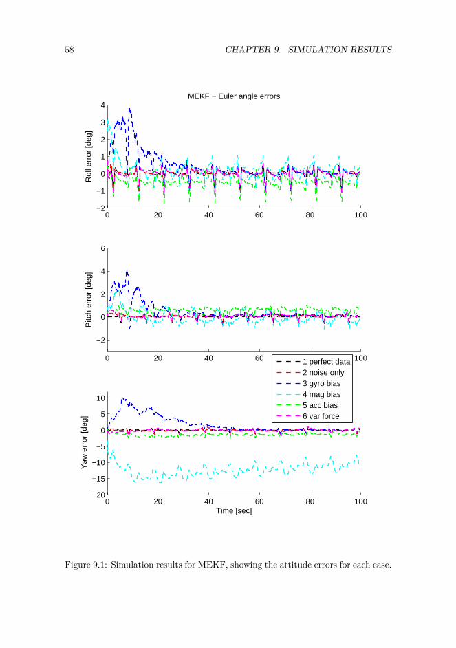
58 CHAPTER 9. SIMULATION RESULTS
0 20 40 60 80 100−2
−1
0
1
2
3
4MEKF − Euler angle errors
Rol
l err
or [d
eg]
0 20 40 60 80 100
−2
0
2
4
6
Pitc
h er
ror
[deg
]
0 20 40 60 80 100−20
−15
−10
−5
0
5
10
Time [sec]
Yaw
err
or [d
eg]
1 perfect data2 noise only3 gyro bias4 mag bias5 acc bias6 var force
Figure 9.1: Simulation results for MEKF, showing the attitude errors for each case.
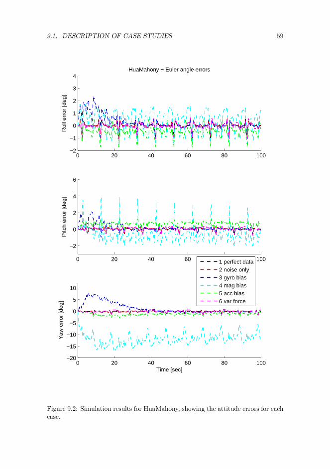
9.1. DESCRIPTION OF CASE STUDIES 59
0 20 40 60 80 100−2
−1
0
1
2
3
4HuaMahony − Euler angle errors
Rol
l err
or [d
eg]
0 20 40 60 80 100
−2
0
2
4
6
Pitc
h er
ror
[deg
]
0 20 40 60 80 100−20
−15
−10
−5
0
5
10
Time [sec]
Yaw
err
or [d
eg]
1 perfect data2 noise only3 gyro bias4 mag bias5 acc bias6 var force
Figure 9.2: Simulation results for HuaMahony, showing the attitude errors for eachcase.
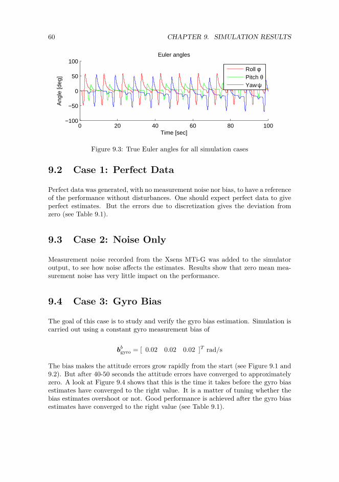
60 CHAPTER 9. SIMULATION RESULTS
0 20 40 60 80 100−100
−50
0
50
100Euler angles
Time [sec]
Ang
le [d
eg]
Roll φPitch θYaw ψ
Figure 9.3: True Euler angles for all simulation cases
9.2 Case 1: Perfect Data
Perfect data was generated, with no measurement noise nor bias, to have a referenceof the performance without disturbances. One should expect perfect data to giveperfect estimates. But the errors due to discretization gives the deviation fromzero (see Table 9.1).
9.3 Case 2: Noise Only
Measurement noise recorded from the Xsens MTi-G was added to the simulatoroutput, to see how noise affects the estimates. Results show that zero mean mea-surement noise has very little impact on the performance.
9.4 Case 3: Gyro Bias
The goal of this case is to study and verify the gyro bias estimation. Simulation iscarried out using a constant gyro measurement bias of
bbgyro = [ 0.02 0.02 0.02 ]T rad/s
The bias makes the attitude errors grow rapidly from the start (see Figure 9.1 and9.2). But after 40-50 seconds the attitude errors have converged to approximatelyzero. A look at Figure 9.4 shows that this is the time it takes before the gyro biasestimates have converged to the right value. It is a matter of tuning whether thebias estimates overshoot or not. Good performance is achieved after the gyro biasestimates have converged to the right value (see Table 9.1).
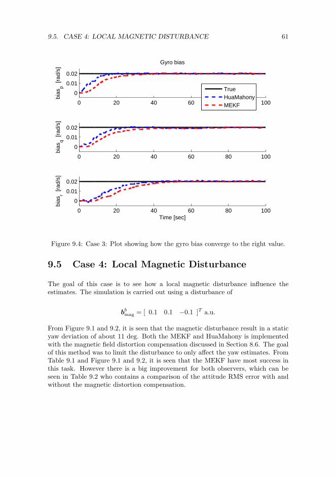
9.5. CASE 4: LOCAL MAGNETIC DISTURBANCE 61
0 20 40 60 80 100
0
0.01
0.02
Gyro biasbi
asp [
rad/
s]
TrueHuaMahonyMEKF
0 20 40 60 80 100
0
0.01
0.02
bias
q [ra
d/s]
0 20 40 60 80 100
0
0.01
0.02
bias
r [ra
d/s]
Time [sec]
Figure 9.4: Case 3: Plot showing how the gyro bias converge to the right value.
9.5 Case 4: Local Magnetic Disturbance
The goal of this case is to see how a local magnetic disturbance influence theestimates. The simulation is carried out using a disturbance of
bbmag = [ 0.1 0.1 −0.1 ]T a.u.
From Figure 9.1 and 9.2, it is seen that the magnetic disturbance result in a staticyaw deviation of about 11 deg. Both the MEKF and HuaMahony is implementedwith the magnetic field distortion compensation discussed in Section 8.6. The goalof this method was to limit the disturbance to only affect the yaw estimates. FromTable 9.1 and Figure 9.1 and 9.2, it is seen that the MEKF have most success inthis task. However there is a big improvement for both observers, which can beseen in Table 9.2 who contains a comparison of the attitude RMS error with andwithout the magnetic distortion compensation.
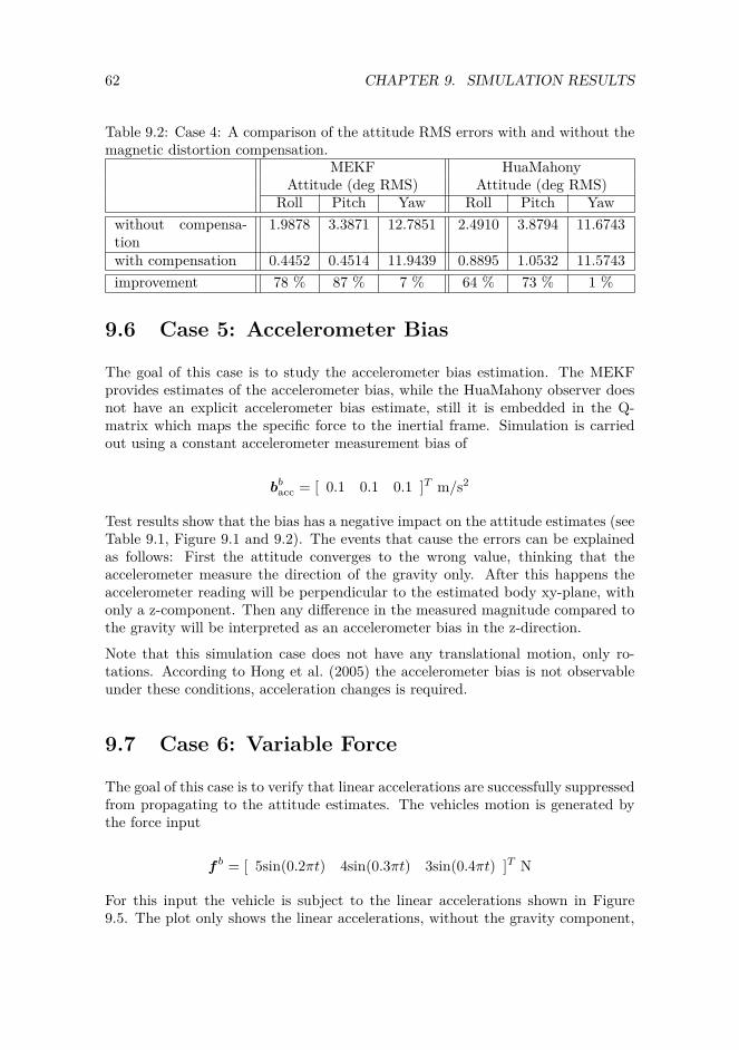
62 CHAPTER 9. SIMULATION RESULTS
Table 9.2: Case 4: A comparison of the attitude RMS errors with and without themagnetic distortion compensation.
MEKF HuaMahonyAttitude (deg RMS) Attitude (deg RMS)
Roll Pitch Yaw Roll Pitch Yawwithout compensa-tion
1.9878 3.3871 12.7851 2.4910 3.8794 11.6743
with compensation 0.4452 0.4514 11.9439 0.8895 1.0532 11.5743improvement 78 % 87 % 7 % 64 % 73 % 1 %
9.6 Case 5: Accelerometer Bias
The goal of this case is to study the accelerometer bias estimation. The MEKFprovides estimates of the accelerometer bias, while the HuaMahony observer doesnot have an explicit accelerometer bias estimate, still it is embedded in the Q-matrix which maps the specific force to the inertial frame. Simulation is carriedout using a constant accelerometer measurement bias of
bbacc = [ 0.1 0.1 0.1 ]T m/s2
Test results show that the bias has a negative impact on the attitude estimates (seeTable 9.1, Figure 9.1 and 9.2). The events that cause the errors can be explainedas follows: First the attitude converges to the wrong value, thinking that theaccelerometer measure the direction of the gravity only. After this happens theaccelerometer reading will be perpendicular to the estimated body xy-plane, withonly a z-component. Then any difference in the measured magnitude compared tothe gravity will be interpreted as an accelerometer bias in the z-direction.
Note that this simulation case does not have any translational motion, only ro-tations. According to Hong et al. (2005) the accelerometer bias is not observableunder these conditions, acceleration changes is required.
9.7 Case 6: Variable Force
The goal of this case is to verify that linear accelerations are successfully suppressedfrom propagating to the attitude estimates. The vehicles motion is generated bythe force input
f b = [ 5sin(0.2πt) 4sin(0.3πt) 3sin(0.4πt) ]T N
For this input the vehicle is subject to the linear accelerations shown in Figure9.5. The plot only shows the linear accelerations, without the gravity component,
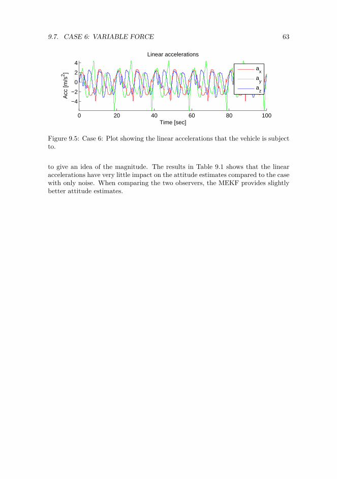
9.7. CASE 6: VARIABLE FORCE 63
0 20 40 60 80 100
−4
−2
0
2
4
Linear accelerations
Time [sec]
Acc
[m/s
2 ]
a
x
ay
az
Figure 9.5: Case 6: Plot showing the linear accelerations that the vehicle is subjectto.
to give an idea of the magnitude. The results in Table 9.1 shows that the linearaccelerations have very little impact on the attitude estimates compared to the casewith only noise. When comparing the two observers, the MEKF provides slightlybetter attitude estimates.

64 CHAPTER 9. SIMULATION RESULTS
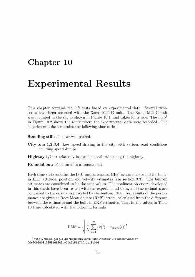
Chapter 10
Experimental Results
This chapter contains real life tests based on experimental data. Several time-series have been recorded with the Xsens MTi-G unit. The Xsens MTi-G unitwas mounted in the car as shown in Figure 10.1, and taken for a ride. The map1
in Figure 10.2 shows the route where the experimental data were recorded. Theexperimental data contains the following time-series:
Standing still: The car was parked.
City tour 1,2,3,4: Low speed driving in the city with various road conditionsincluding speed dumps
Highway 1,2: A relatively fast and smooth ride along the highway.
Roundabout: Four turns in a roundabout.
Each time-serie contains the IMU measurements, GPS measurements and the built-in EKF attitude, position and velocity estimates (see section 3.3). The built-inestimates are considered to be the true values. The nonlinear observers developedin this thesis have been tested with the experimental data, and the estimates arecompared to the estimates provided by the built-in EKF. Test results of the perfor-mance are given as Root Mean Square (RMS) errors, calculated from the differencebetween the estimates and the built-in EKF estimates. That is, the values in Table10.1 are calculated with the following formula
RMS =
√√√√ 1N
N∑i=1
(x(i)− xxsens(i))2
1http://maps.google.no/maps/ms?ie=UTF8&hl=no&oe=UTF8&msa=0&msid=206709540317555168643.00049c56274f1dc13c01d
65
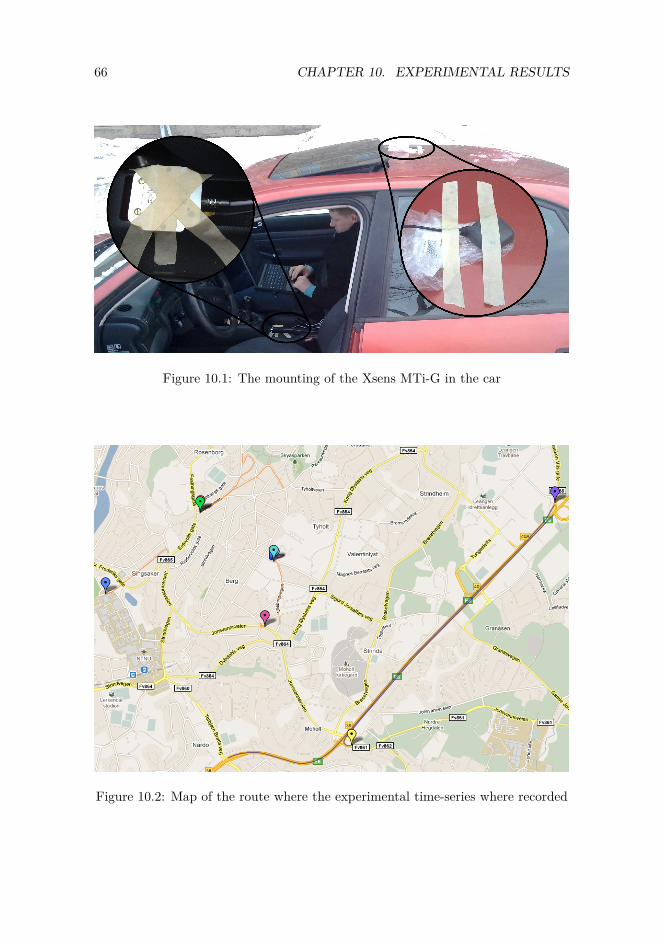
66 CHAPTER 10. EXPERIMENTAL RESULTS
Figure 10.1: The mounting of the Xsens MTi-G in the car
Figure 10.2: Map of the route where the experimental time-series where recorded
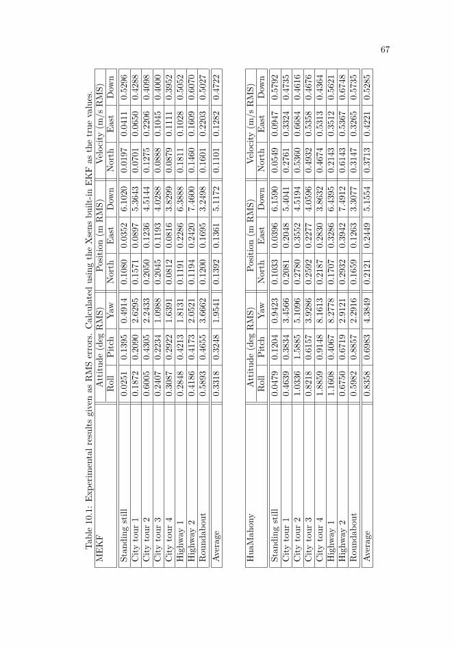
67
Table10.1:Ex
perim
entalr
esults
givenas
RMSerrors.CalculatedusingtheXsens
built-in
EKFas
thetrue
values.
MEK
FAttitu
de(deg
RMS)
Posit
ion(m
RMS)
Velocity
(m/s
RMS)
Roll
Pitch
Yaw
North
East
Dow
nNorth
East
Dow
nStan
ding
still
0.0251
0.1395
0.4914
0.1080
0.0352
6.1020
0.0197
0.0411
0.5296
City
tour
10.1872
0.2090
2.6295
0.1571
0.0897
5.3643
0.0701
0.0650
0.4288
City
tour
20.6005
0.4305
2.2433
0.2050
0.1236
4.5144
0.1275
0.2206
0.4098
City
tour
30.2407
0.2234
1.0988
0.2045
0.1193
4.0288
0.0888
0.1045
0.4000
City
tour
40.3087
0.2922
1.6391
0.0812
0.0816
3.8299
0.0879
0.1111
0.3952
Highw
ay1
0.2848
0.4213
1.8131
0.1191
0.2286
6.3888
0.1811
0.1028
0.5052
Highw
ay2
0.4186
0.4173
2.0521
0.1194
0.2420
7.4600
0.1460
0.1609
0.6070
Rou
ndab
out
0.5893
0.4655
3.6662
0.1200
0.1695
3.2498
0.1601
0.2203
0.5027
Average
0.3318
0.3248
1.9541
0.1392
0.1361
5.1172
0.1101
0.1282
0.4722
Hua
Mah
ony
Attitu
de(deg
RMS)
Posit
ion(m
RMS)
Velocity
(m/s
RMS)
Roll
Pitch
Yaw
North
East
Dow
nNorth
East
Dow
nStan
ding
still
0.0479
0.1204
0.9423
0.1033
0.0396
6.1590
0.0549
0.0947
0.5792
City
tour
10.4639
0.3834
3.4566
0.2081
0.2048
5.4041
0.2761
0.3324
0.4735
City
tour
21.0336
1.5885
5.1096
0.2780
0.3552
4.5194
0.5360
0.6684
0.4616
City
tour
30.8218
0.6157
3.9286
0.2592
0.2277
4.0596
0.4932
0.5358
0.4676
City
tour
41.8859
0.9148
8.1613
0.2187
0.2830
3.8632
0.4674
0.5313
0.4364
Highw
ay1
1.1608
0.4067
8.2778
0.1707
0.3286
6.4395
0.2143
0.3512
0.5621
Highw
ay2
0.6750
0.6719
2.9121
0.2932
0.3942
7.4912
0.6143
0.5367
0.6748
Rou
ndab
out
0.5982
0.8857
2.2916
0.1659
0.1263
3.3077
0.3147
0.3265
0.5735
Average
0.8358
0.6983
4.3849
0.2121
0.2449
5.1554
0.3713
0.4221
0.5285
68 CHAPTER 10. EXPERIMENTAL RESULTS
where N is the number of samples in the time-serie, and x represent roll, pitch andso on. The first 10 seconds have been omitted in the RMS calculation to removemost of the transient part. Tests have been carried out for the following observers:
MEKF is the multiplicative extended Kalman filter including attitude, positionand velocity estimates. The filter was derived with two different measurementequations; one using the q-method and the other using vectorial measurements. Ifnothing else is specified, the vectorial measurement equation is used. The followingKalman filter tuning matrices have been used
Qk = diag( 5e-71×3 1e-91×3 1e-01×3 7e-41×3 1e-71×3 )Rk = diag( 1e-41×3 7e-21×3 1e-11×3 5e-41×3 )P0 = diag( 1e-51×3 1e-91×3 1e-01×3 1e-31×3 1e-81×3 )
HuaMahony is the nonlinear observer combination of Hua (2010) and Mahonyet al. (2008) including attitude, position and velocity estimates. The discrete-time corrector-predictor formulation of HuaMahony has been implemented. Thefollowing observer gains have been used
Kquat = 0.5 · h, Kbgyr = 0.002 · h, kmag = 0.26, kacc = 1kpos = 1 · 25h, kvel = 1 · 25h, kQ = 0.12 · 25h
where h is the sample time. Values used for the magnetic declination, gravity andlever arm are:
Declination = 0.0323 radgn = [ 0 0 9.81 ]T m/s2
rbant = [ −0.65 −0.08 −0.90 ]T m
10.1 Main Results
The experimental results for each time-serie are given in Table 10.1. Results showthat the MEKF has an average better performance compared to the HuaMahonyobserver.
The MEKF has an average error in roll, pitch and yaw of 0.3, 0.3 and 1.9 degrespectively. Considering the accuracy of the “true” value (see Table 3.2), this is avery good result. The HuaMahony observer has an average error in roll, pitch andyaw of 0.8, 0.6 and 4.3 deg respectively. Roll an pitch estimates must be said to have
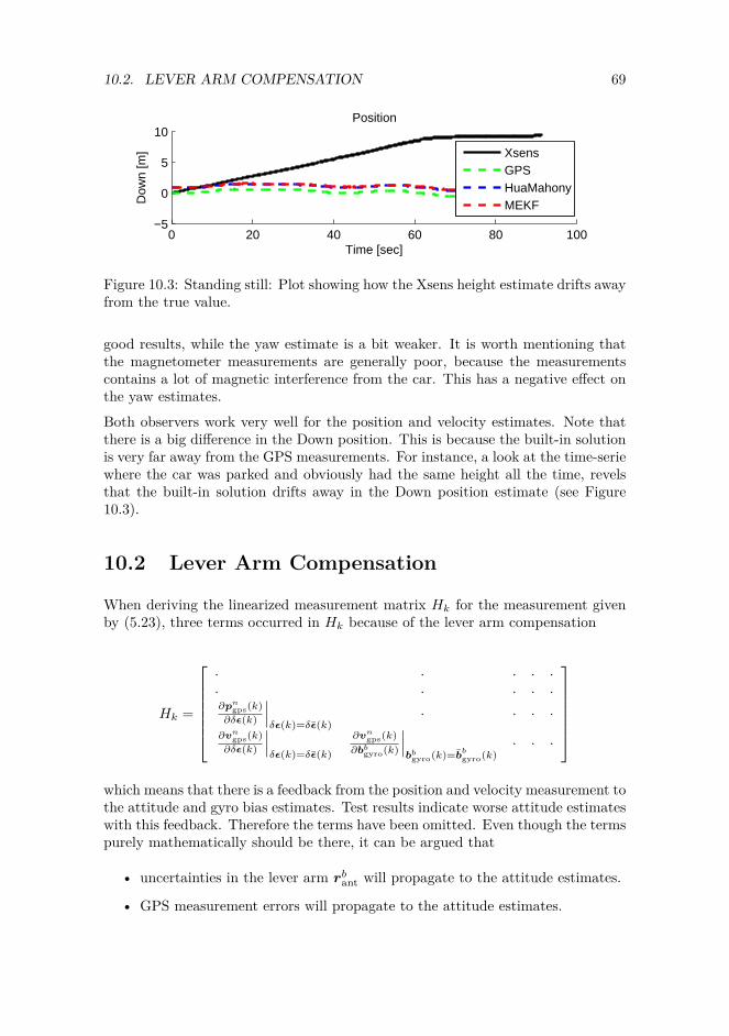
10.2. LEVER ARM COMPENSATION 69
0 20 40 60 80 100−5
0
5
10Position
Time [sec]
Dow
n [m
]
XsensGPSHuaMahonyMEKF
Figure 10.3: Standing still: Plot showing how the Xsens height estimate drifts awayfrom the true value.
good results, while the yaw estimate is a bit weaker. It is worth mentioning thatthe magnetometer measurements are generally poor, because the measurementscontains a lot of magnetic interference from the car. This has a negative effect onthe yaw estimates.
Both observers work very well for the position and velocity estimates. Note thatthere is a big difference in the Down position. This is because the built-in solutionis very far away from the GPS measurements. For instance, a look at the time-seriewhere the car was parked and obviously had the same height all the time, revelsthat the built-in solution drifts away in the Down position estimate (see Figure10.3).
10.2 Lever Arm Compensation
When deriving the linearized measurement matrix Hk for the measurement givenby (5.23), three terms occurred in Hk because of the lever arm compensation
Hk =
· · · · ·· · · · ·∂pn
gps(k)∂δε(k)
∣∣∣δε(k)=δε(k)
· · · ·∂vn
gps(k)∂δε(k)
∣∣∣δε(k)=δε(k)
∂vngps(k)
∂bbgyro(k)
∣∣∣bb
gyro(k)=bbgyro(k)
· · ·
which means that there is a feedback from the position and velocity measurement tothe attitude and gyro bias estimates. Test results indicate worse attitude estimateswith this feedback. Therefore the terms have been omitted. Even though the termspurely mathematically should be there, it can be argued that
• uncertainties in the lever arm rbant will propagate to the attitude estimates.
• GPS measurement errors will propagate to the attitude estimates.
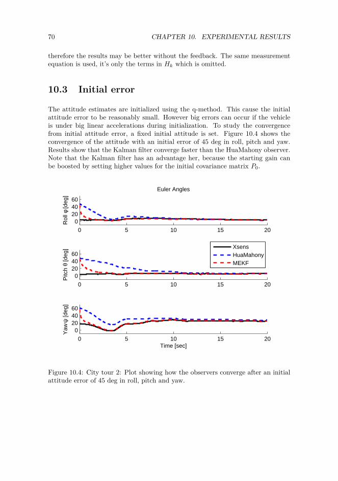
70 CHAPTER 10. EXPERIMENTAL RESULTS
therefore the results may be better without the feedback. The same measurementequation is used, it’s only the terms in Hk which is omitted.
10.3 Initial error
The attitude estimates are initialized using the q-method. This cause the initialattitude error to be reasonably small. However big errors can occur if the vehicleis under big linear accelerations during initialization. To study the convergencefrom initial attitude error, a fixed initial attitude is set. Figure 10.4 shows theconvergence of the attitude with an initial error of 45 deg in roll, pitch and yaw.Results show that the Kalman filter converge faster than the HuaMahony observer.Note that the Kalman filter has an advantage her, because the starting gain canbe boosted by setting higher values for the initial covariance matrix P0.
0 5 10 15 20
0204060
Euler Angles
Rol
l φ [d
eg]
0 5 10 15 20
0204060
Pitc
h θ
[deg
]
XsensHuaMahonyMEKF
0 5 10 15 20
0204060
Yaw
ψ [d
eg]
Time [sec]
Figure 10.4: City tour 2: Plot showing how the observers converge after an initialattitude error of 45 deg in roll, pitch and yaw.
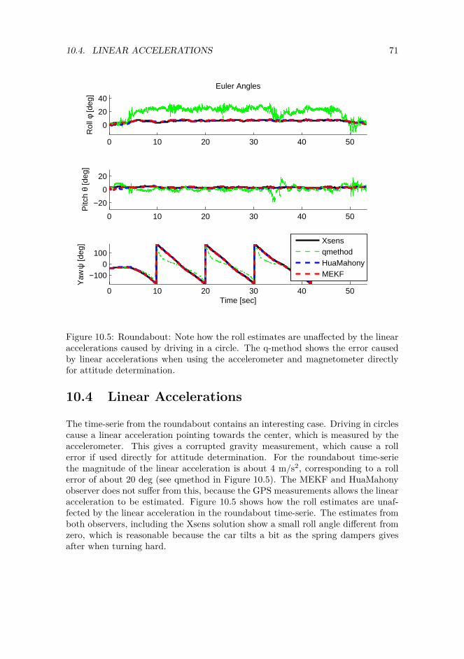
10.4. LINEAR ACCELERATIONS 71
0 10 20 30 40 50
0
20
40
Euler AnglesR
oll φ
[deg
]
0 10 20 30 40 50
−20
0
20
Pitc
h θ
[deg
]
0 10 20 30 40 50
−1000
100
Time [sec]
Yaw
ψ [d
eg]
XsensqmethodHuaMahonyMEKF
Figure 10.5: Roundabout: Note how the roll estimates are unaffected by the linearaccelerations caused by driving in a circle. The q-method shows the error causedby linear accelerations when using the accelerometer and magnetometer directlyfor attitude determination.
10.4 Linear Accelerations
The time-serie from the roundabout contains an interesting case. Driving in circlescause a linear acceleration pointing towards the center, which is measured by theaccelerometer. This gives a corrupted gravity measurement, which cause a rollerror if used directly for attitude determination. For the roundabout time-seriethe magnitude of the linear acceleration is about 4 m/s2, corresponding to a rollerror of about 20 deg (see qmethod in Figure 10.5). The MEKF and HuaMahonyobserver does not suffer from this, because the GPS measurements allows the linearacceleration to be estimated. Figure 10.5 shows how the roll estimates are unaf-fected by the linear acceleration in the roundabout time-serie. The estimates fromboth observers, including the Xsens solution show a small roll angle different fromzero, which is reasonable because the car tilts a bit as the spring dampers givesafter when turning hard.
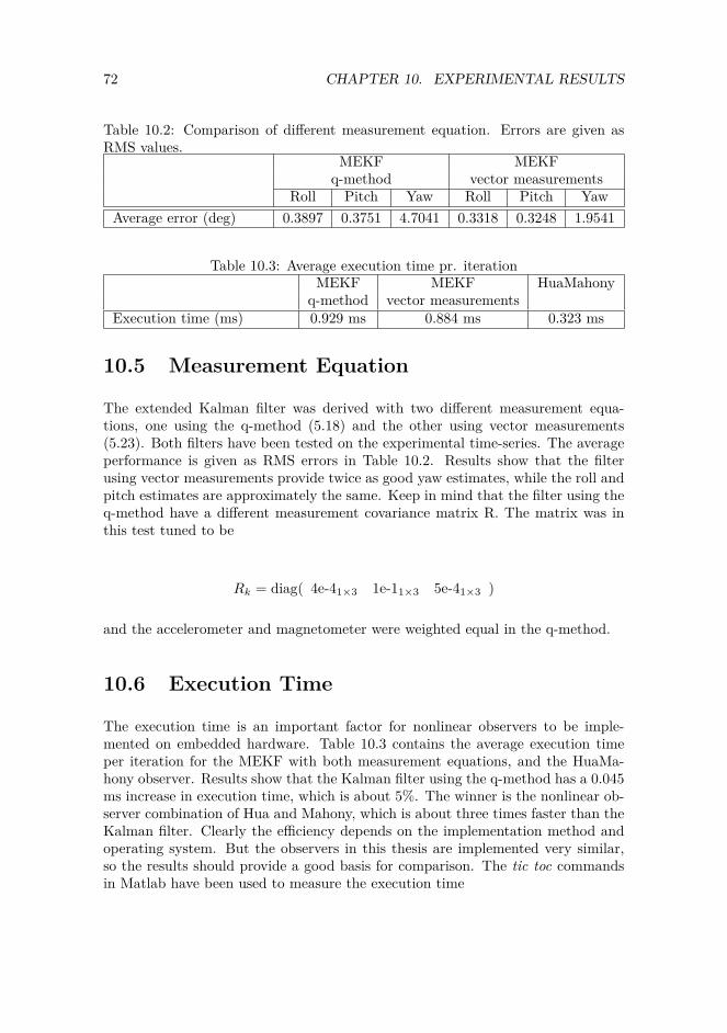
72 CHAPTER 10. EXPERIMENTAL RESULTS
Table 10.2: Comparison of different measurement equation. Errors are given asRMS values.
MEKF MEKFq-method vector measurements
Roll Pitch Yaw Roll Pitch YawAverage error (deg) 0.3897 0.3751 4.7041 0.3318 0.3248 1.9541
Table 10.3: Average execution time pr. iterationMEKF MEKF HuaMahony
q-method vector measurementsExecution time (ms) 0.929 ms 0.884 ms 0.323 ms
10.5 Measurement Equation
The extended Kalman filter was derived with two different measurement equa-tions, one using the q-method (5.18) and the other using vector measurements(5.23). Both filters have been tested on the experimental time-series. The averageperformance is given as RMS errors in Table 10.2. Results show that the filterusing vector measurements provide twice as good yaw estimates, while the roll andpitch estimates are approximately the same. Keep in mind that the filter using theq-method have a different measurement covariance matrix R. The matrix was inthis test tuned to be
Rk = diag( 4e-41×3 1e-11×3 5e-41×3 )
and the accelerometer and magnetometer were weighted equal in the q-method.
10.6 Execution Time
The execution time is an important factor for nonlinear observers to be imple-mented on embedded hardware. Table 10.3 contains the average execution timeper iteration for the MEKF with both measurement equations, and the HuaMa-hony observer. Results show that the Kalman filter using the q-method has a 0.045ms increase in execution time, which is about 5%. The winner is the nonlinear ob-server combination of Hua and Mahony, which is about three times faster than theKalman filter. Clearly the efficiency depends on the implementation method andoperating system. But the observers in this thesis are implemented very similar,so the results should provide a good basis for comparison. The tic toc commandsin Matlab have been used to measure the execution time
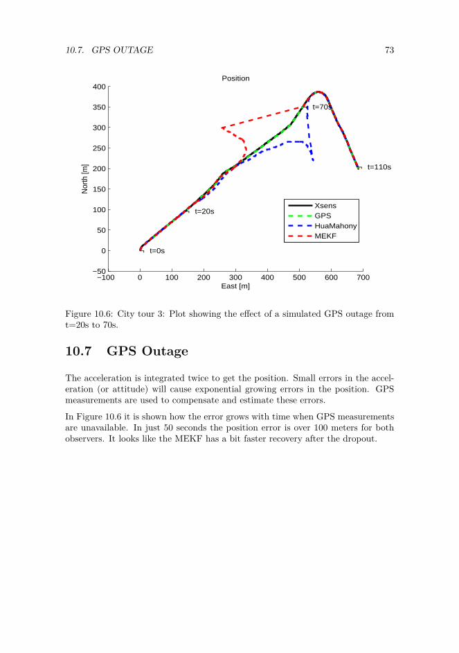
10.7. GPS OUTAGE 73
−100 0 100 200 300 400 500 600 700−50
0
50
100
150
200
250
300
350
400Position
East [m]
Nor
th [m
]
¬ t=0s
¬ t=20s
¬ t=70s
¬ t=110s
XsensGPSHuaMahonyMEKF
Figure 10.6: City tour 3: Plot showing the effect of a simulated GPS outage fromt=20s to 70s.
10.7 GPS Outage
The acceleration is integrated twice to get the position. Small errors in the accel-eration (or attitude) will cause exponential growing errors in the position. GPSmeasurements are used to compensate and estimate these errors.
In Figure 10.6 it is shown how the error grows with time when GPS measurementsare unavailable. In just 50 seconds the position error is over 100 meters for bothobservers. It looks like the MEKF has a bit faster recovery after the dropout.

74 CHAPTER 10. EXPERIMENTAL RESULTS
Chapter 11
Conclusions
Two different nonlinear observers for integration of GNSS and IMU have beenimplemented and tested:
• A quaternion based multiplicative extended Kalman filter, named MEKF
• A nonlinear observer, named HuaMahony.
Simulations have been carried out as a case study to see how different disturbancesaffect the estimates of position, velocity and attitude. The most dominating errorcomes from the local magnetic disturbance, however it has little effect on the rolland pitch estimates thanks to the magnetic distortion compensation. Simulationsresults reveals that the accelerometer bias is unobservable without accelerationchanges. If case 4 is excluded, the average performance is good, showing a dynamicaccuracy of < 0.5 deg RMS for the attitude estimates. Both observers have a verysimilar performance and it is not possible to say anything about which one is better.
Experimental data have been recorded with the Xsens MTi-G unit. Assumingthat the Xsens built-in EKF gives the true values, the average performance for theexperimental test shows an attitude accuracy of (0.3 0.3 2.0) and (0.8 0.7 4.4) degRMS for the MEKF and HuaMahony observer respectively. The results indicatethat the MEKF has the best performance, but it is difficult to be very conclusiveas there is several uncertainties: (i) the performance is depending on the tuning,but an exact equal tuning is difficult to achieve; (ii) there is some uncertainties inthe “true” values provided by the Xsens unit.
However some differences between the MEKF and HuaMahony observer can beemphasized:
• The MEKF has a quicker convergence from initial errors, because of the initialcovariance matrix which is used in the Riccati equation.
75

76 CHAPTER 11. CONCLUSIONS
• The HuaMahony observer is three times faster when it comes to executiontime. The test was performed in Matlab, which is known to efficiently han-dle matrix calculations, therefore one may expect an even bigger ratio forimplementation on embedded hardware.
Chapter 12
Further Work
Estimation of the yaw angle is the most challenging part. The accuracy of the yawestimate may be improved by making a no-sideslip assumption. This means that anassumption is made about zero velocity along the body-fixed y-axis. Consequently,the measured velocity will contain information about the yaw angle. However thisassumption is most suited for vehicles subject to none or short term sidewardsslipping, such as automotive vehicles (Xsens 2009d).
For aerial vehicles there are several actions that might be done to improve re-dundancy and accuracy. For instance integrating a barometer which measure thealtitude, or a dynamic pressure sensor to measure airspeed. Also an applicationspecific dynamic model of the vehicle can be integrated, which can limit the dy-namics of the movement (Koifman and Bar-Itzhack 1999). The drawback is theloss of generality.
Adaptive tuning of the observer gains may also be considered for increased per-formance. For the multiplicative extended Kalman filter this may be achieved bymanipulating the measurement covariance matrix R (Cheng et al. 2008).
77

78 CHAPTER 12. FURTHER WORK
Bibliography
Abdel-Hafez, M. F. (2010). The autocovariance least-squares technique for gpsmeasurement noise estimation, IEEE Transactions on Vehicular Technology59(2): 574–588.
Babu, R., Wang, J. and Rao, G. (2008). Analysis of ultra-tight gps/ins integratedsystem for navigation performance, IEEE-ICSCN pp. 234–237.
Bar-Itzhack, I. Y. (1996). Request: A recursive quest algorithm for sequential atti-tude determination, Journal of Guidance, Control, and Dynamics 19(5): 1034–1038.
Cheng, L., Zhaoying, Z. and Xu, F. (2008). Attitude determination for mavs usinga kalman filter, Tsinghua Science and Technology 13(5): 593–597.
Crassidis, J. L., Markley, F. L. and Cheng, Y. (2007). A survey of nonlinear at-titude estimation methods, AIAA Journal of Guidance, Control, and Dynamics30(1): 11–28.
Egeland, O. and Gravdahl, J. T. (2003). Modeling and Simulation for AutomaticControl, 2nd edn, Marine Cybernetics AS.
Ellingsen, H. (2008). Development of a low-cost integrated navigation system forusvs, Master’s thesis, Norwegian University of Science and Technology.
Fiorenzani, T., Manes, C., Oriolo, G. and Peliti, P. (2008). Comparative study ofunscented kalman filter and extended kalman filter for position/attitude estima-tion in unmanned aerial vehicles.
Fossen, T. I. (2011). Handbook of Marine Craft Hydrodynamics and Motion Control,John Wiley & Sons Ltd.
Gade, K. (2009). Introduction to inertial navigation and kalman filtering, Tutorialfor: IAIN World Congress, Stockholm .
Hong, S., Lee, M. H., Chun, H.-H., Kwon, S.-H. and Speyer, J. L. (2005). Observ-ability of error states in gps/ins integration, IEEE Transactions on VehicularTechnology 54(2): 731–743.
79
80 BIBLIOGRAPHY
Hua, M.-D. (2010). Attitude estimation for accelerated vehicles using gps/ins mea-surements, Control Engineering Practice 18: 723–732.
Jouffroy, J. and Fossen, T. (2010). A tutorial on incremental stability analysisusing contraction theory, Modeling, Identication and Control 31(3): 93–106.
Keat, J. E. (1977). Analysis of least-squares attitude determination routine doaop,Computer Sciences Corp. Report CSC/TM-77/6034.
Koifman, M. and Bar-Itzhack, I. (1999). Inertial navigation system aided by aircraftdynamics, IEEE Transactions on Control System Technology 7(4): 487–493.
Lefferts, E. J. and Schuster, M. D. (1982). Kalman filtering for spacecraft attitudeestimation, Journal of Navigation, Control and Dynamics JGCD-5(5): 417–428.
Lerner, G. (1978). Three-axis attitude determination, Spacecraft Attitude Deter-mination and Control pp. 420–428.
Madgwick, S. O. (2010). An efficient orientation filter for inertial and inertial/-magnetic sensor arrays.
Mahony, R., Hamel, T. and Pflimlin, J.-M. (2008). Nonlinear complementary filterson the special orthogonal group ., IEEE Transactions on Automatic Control53(5): 1203–1218.
Markley, F. L. (2003). Attitude error representations for kalman filtering, Journalof Guidance, Control, and Dynamics 26(2): 311–317.
Martin, P. and Salaün, E. (2008). An invariant observer for earth-velocity-aidedattitude heading reference systems, In IFAC World Congress 17: 9857–9864.
Maybeck, P. S. (1979). Stochastic Models, Estimation and Control Vol. 1, AcademicPress.
Nocedal, J. and Wright, S. J. (2006). Numerical Optimization, 2nd edn, Springer.
Schmidt, G. and Phillips, R. (2010). Ins/gps integration architectures, NATO RTOLecture Series RTO-EN-SET-116.
Shuster, M. D. and Oh, S. (1981). Three-axis attitude determination from vectorobservations, Journal of Guidance and Control 4(1): 70–77.
Vasconcelos, J. F., Cardeira, B., Silvestre, C., Oliveira, P. and Batista, P. (2011).Discrete-time complementary filters for attitude and position estimation: De-sign, analysis and experimental validation, IEEE Transactions on Control Sys-tem Technology 19(1): 181–198.
Vasconcelos, J., Silvestre, C. and Oliveira, P. (2011). Ins/gps aided by frequencycontents of vector observations with application to autonomous surface crafts,IEEE Journal of Oceanic Engineering 36(2): 347–363.
BIBLIOGRAPHY 81
Vik, B. (n.d.). Integrated satellite and inertial navigation systems. Lecture notes,Department of Engineering Cybernetics, Norwegian University of Science andTechnology.
Vik, B. and Fossen, T. I. (2001). A nonlinear observer for gps and ins integra-tion, Proceedings of the Conference on Decision and Control, Orlando, Floridapp. 2956–2961.
Wahba, G. (1965). A least squares estimate of satellite attitude, SIAM Review7(3): 409.
Wendel, J. and Trommer, G. F. (2004). Tightly coupled gps/ins integration formissile applications, Aerospace Science and Technology 8: 627–634.
Wenstad, P. (2010). Gps guided r/c car, Master’s thesis, Norwegian University ofScience and Technology.
Xsens (2009a). Magnetic Field Mapper Documentation. Revision E.
Xsens (2009b). MT Low-Level Communication Protocol Documentation. RevisionK.
Xsens (2009c). MT Manager User Manual. Revision F.
Xsens (2009d). MTi-G User Manual and Technical Documentation. Revision G.
Yi, Y. and Grejner-Brzezinska, D. (2006). Tightly-coupled gps/ins integration usingunscented kalman filter and particle filter, Proceedings of the 19th InternationalTechnical Meeting of the Satellite Division of The Institute of Navigation (IONGNSS 2006) pp. 2182–2191.

82 BIBLIOGRAPHY
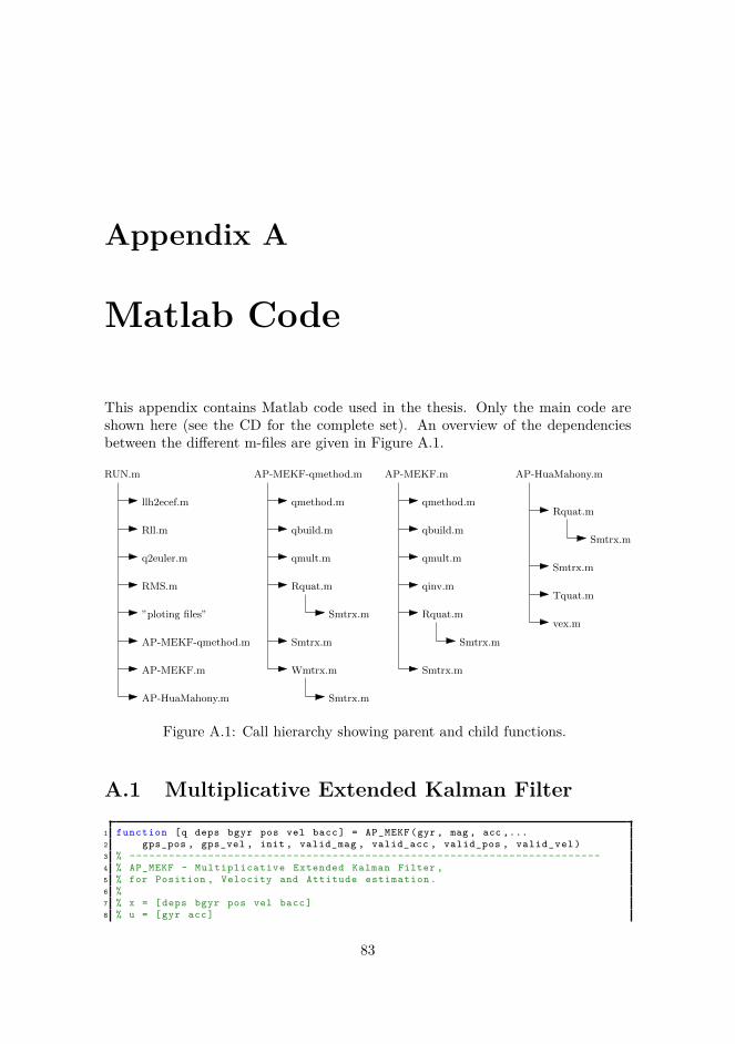
Appendix A
Matlab Code
This appendix contains Matlab code used in the thesis. Only the main code areshown here (see the CD for the complete set). An overview of the dependenciesbetween the different m-files are given in Figure A.1.
AP-MEKF.m
qmethod.m
qbuild.m
qmult.m
Rquat.m
Smtrx.m
Smtrx.m
qinv.m
AP-HuaMahony.m
Rquat.m
Smtrx.m
Smtrx.m
Tquat.m
vex.m
AP-MEKF-qmethod.m
qmethod.m
qbuild.m
qmult.m
Rquat.m
Smtrx.m
Wmtrx.m
Smtrx.m
Smtrx.m
RUN.m
llh2ecef.m
Rll.m
q2euler.m
RMS.m
”ploting files”
AP-MEKF-qmethod.m
AP-MEKF.m
AP-HuaMahony.m
Figure A.1: Call hierarchy showing parent and child functions.
A.1 Multiplicative Extended Kalman Filter
1 function [q deps bgyr pos vel bacc] = AP_MEKF (gyr , mag , acc ,...2 gps_pos , gps_vel , init , valid_mag , valid_acc , valid_pos , valid_vel )3 % ------------------------------------------------------------------------4 % AP_MEKF - Multiplicative Extended Kalman Filter ,5 % for Position , Velocity and Attitude estimation .6 %7 % x = [deps bgyr pos vel bacc]8 % u = [gyr acc]
83
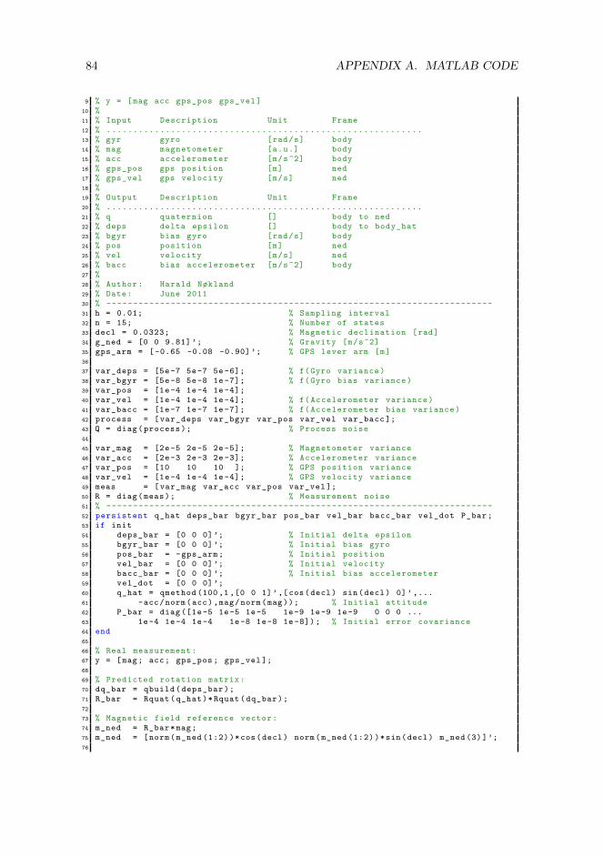
84 APPENDIX A. MATLAB CODE
9 % y = [mag acc gps_pos gps_vel ]10 %11 % Input Description Unit Frame12 % ...........................................................13 % gyr gyro [rad/s] body14 % mag magnetometer [a.u.] body15 % acc accelerometer [m/s^2] body16 % gps_pos gps position [m] ned17 % gps_vel gps velocity [m/s] ned18 %19 % Output Description Unit Frame20 % ...........................................................21 % q quaternion [] body to ned22 % deps delta epsilon [] body to body_hat23 % bgyr bias gyro [rad/s] body24 % pos position [m] ned25 % vel velocity [m/s] ned26 % bacc bias accelerometer [m/s^2] body27 %28 % Author : Harald Nøkland29 % Date: June 201130 % ------------------------------------------------------------------------31 h = 0.01; % Sampling interval32 n = 15; % Number of states33 decl = 0.0323; % Magnetic declination [rad]34 g_ned = [0 0 9.81] ’; % Gravity [m/s^2]35 gps_arm = [ -0.65 -0.08 -0.90] ’; % GPS lever arm [m]36
37 var_deps = [5e -7 5e -7 5e -6]; % f(Gyro variance )38 var_bgyr = [5e -8 5e -8 1e -7]; % f(Gyro bias variance )39 var_pos = [1e -4 1e -4 1e -4];40 var_vel = [1e -4 1e -4 1e -4]; % f( Accelerometer variance )41 var_bacc = [1e -7 1e -7 1e -7]; % f( Accelerometer bias variance )42 process = [ var_deps var_bgyr var_pos var_vel var_bacc ];43 Q = diag( process ); % Process noise44
45 var_mag = [2e -5 2e -5 2e -5]; % Magnetometer variance46 var_acc = [2e -3 2e -3 2e -3]; % Accelerometer variance47 var_pos = [10 10 10 ]; % GPS position variance48 var_vel = [1e -4 1e -4 1e -4]; % GPS velocity variance49 meas = [ var_mag var_acc var_pos var_vel ];50 R = diag(meas); % Measurement noise51 % ------------------------------------------------------------------------52 persistent q_hat deps_bar bgyr_bar pos_bar vel_bar bacc_bar vel_dot P_bar ;53 if init54 deps_bar = [0 0 0] ’; % Initial delta epsilon55 bgyr_bar = [0 0 0] ’; % Initial bias gyro56 pos_bar = -gps_arm ; % Initial position57 vel_bar = [0 0 0] ’; % Initial velocity58 bacc_bar = [0 0 0] ’; % Initial bias accelerometer59 vel_dot = [0 0 0] ’;60 q_hat = qmethod (100 ,1 ,[0 0 1]’,[ cos(decl) sin(decl) 0] ’ ,...61 -acc/norm(acc),mag/norm(mag)); % Initial attitude62 P_bar = diag ([1e -5 1e -5 1e -5 1e -9 1e -9 1e -9 0 0 0 ...63 1e -4 1e -4 1e -4 1e -8 1e -8 1e -8]); % Initial error covariance64 end65
66 % Real measurement :67 y = [mag; acc; gps_pos ; gps_vel ];68
69 % Predicted rotation matrix :70 dq_bar = qbuild ( deps_bar );71 R_bar = Rquat ( q_hat )* Rquat ( dq_bar );72
73 % Magnetic field reference vector :74 m_ned = R_bar *mag;75 m_ned = [norm( m_ned (1:2) )*cos(decl) norm( m_ned (1:2) )*sin(decl) m_ned (3) ]’;76
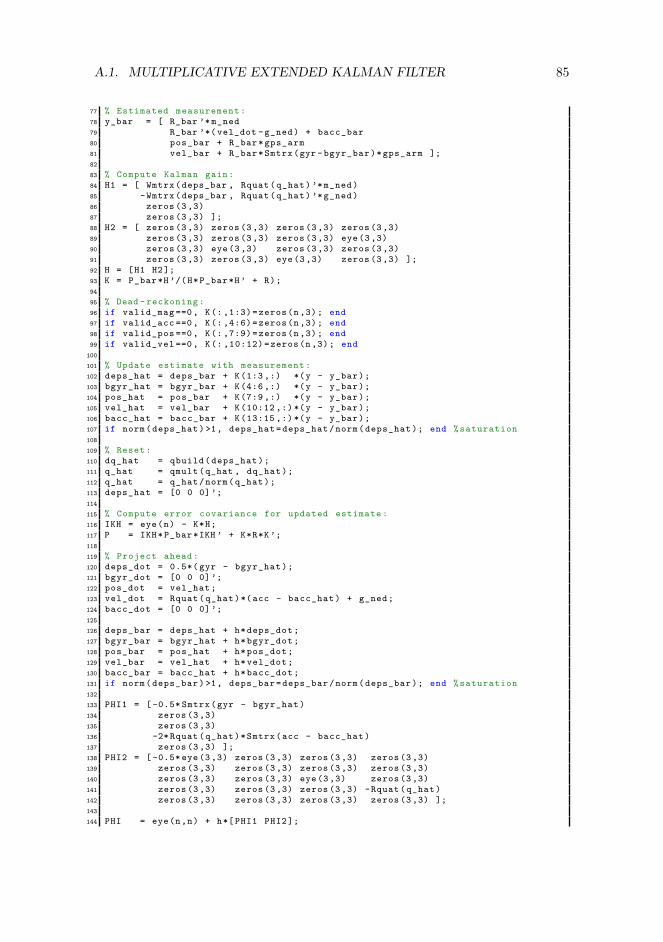
A.1. MULTIPLICATIVE EXTENDED KALMAN FILTER 85
77 % Estimated measurement :78 y_bar = [ R_bar ’* m_ned79 R_bar ’*( vel_dot - g_ned ) + bacc_bar80 pos_bar + R_bar * gps_arm81 vel_bar + R_bar * Smtrx (gyr - bgyr_bar )* gps_arm ];82
83 % Compute Kalman gain:84 H1 = [ Wmtrx (deps_bar , Rquat ( q_hat ) ’* m_ned )85 -Wmtrx (deps_bar , Rquat ( q_hat ) ’* g_ned )86 zeros (3 ,3)87 zeros (3 ,3) ];88 H2 = [ zeros (3 ,3) zeros (3 ,3) zeros (3 ,3) zeros (3 ,3)89 zeros (3 ,3) zeros (3 ,3) zeros (3 ,3) eye (3 ,3)90 zeros (3 ,3) eye (3 ,3) zeros (3 ,3) zeros (3 ,3)91 zeros (3 ,3) zeros (3 ,3) eye (3 ,3) zeros (3 ,3) ];92 H = [H1 H2 ];93 K = P_bar *H ’/(H* P_bar *H’ + R);94
95 % Dead - reckoning :96 if valid_mag ==0 , K(: ,1:3)= zeros (n ,3); end97 if valid_acc ==0 , K(: ,4:6)= zeros (n ,3); end98 if valid_pos ==0 , K(: ,7:9)= zeros (n ,3); end99 if valid_vel ==0 , K(: ,10:12)= zeros (n ,3); end
100
101 % Update estimate with measurement :102 deps_hat = deps_bar + K(1:3 ,:) *(y - y_bar );103 bgyr_hat = bgyr_bar + K(4:6 ,:) *(y - y_bar );104 pos_hat = pos_bar + K(7:9 ,:) *(y - y_bar );105 vel_hat = vel_bar + K(10:12 ,:) *(y - y_bar );106 bacc_hat = bacc_bar + K(13:15 ,:) *(y - y_bar );107 if norm( deps_hat ) >1, deps_hat = deps_hat /norm( deps_hat ); end % saturation108
109 % Reset :110 dq_hat = qbuild ( deps_hat );111 q_hat = qmult (q_hat , dq_hat );112 q_hat = q_hat /norm( q_hat );113 deps_hat = [0 0 0] ’;114
115 % Compute error covariance for updated estimate :116 IKH = eye(n) - K*H;117 P = IKH* P_bar *IKH ’ + K*R*K ’;118
119 % Project ahead :120 deps_dot = 0.5*( gyr - bgyr_hat );121 bgyr_dot = [0 0 0] ’;122 pos_dot = vel_hat ;123 vel_dot = Rquat ( q_hat )*( acc - bacc_hat ) + g_ned ;124 bacc_dot = [0 0 0] ’;125
126 deps_bar = deps_hat + h* deps_dot ;127 bgyr_bar = bgyr_hat + h* bgyr_dot ;128 pos_bar = pos_hat + h* pos_dot ;129 vel_bar = vel_hat + h* vel_dot ;130 bacc_bar = bacc_hat + h* bacc_dot ;131 if norm( deps_bar ) >1, deps_bar = deps_bar /norm( deps_bar ); end % saturation132
133 PHI1 = [ -0.5* Smtrx (gyr - bgyr_hat )134 zeros (3 ,3)135 zeros (3 ,3)136 -2* Rquat ( q_hat )* Smtrx (acc - bacc_hat )137 zeros (3 ,3) ];138 PHI2 = [ -0.5* eye (3 ,3) zeros (3 ,3) zeros (3 ,3) zeros (3 ,3)139 zeros (3 ,3) zeros (3 ,3) zeros (3 ,3) zeros (3 ,3)140 zeros (3 ,3) zeros (3 ,3) eye (3 ,3) zeros (3 ,3)141 zeros (3 ,3) zeros (3 ,3) zeros (3 ,3) -Rquat ( q_hat )142 zeros (3 ,3) zeros (3 ,3) zeros (3 ,3) zeros (3 ,3) ];143
144 PHI = eye(n,n) + h*[ PHI1 PHI2 ];
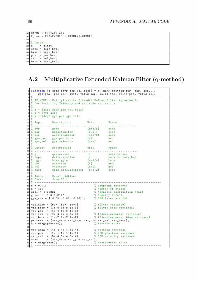
86 APPENDIX A. MATLAB CODE
145 GAMMA = h*eye(n,n);146 P_bar = PHI*P*PHI ’ + GAMMA *Q*GAMMA ’;147
148 % Output :149 q = q_hat ;150 deps = deps_hat ;151 bgyr = bgyr_hat ;152 pos = pos_hat ;153 vel = vel_hat ;154 bacc = bacc_hat ;
A.2 Multiplicative Extended Kalman Filter (q-method)
1 function [q deps bgyr pos vel bacc] = AP_MEKF_qmethod (gyr , mag , acc ,...2 gps_pos , gps_vel , init , valid_mag , valid_acc , valid_pos , valid_vel )3 % ------------------------------------------------------------------------4 % AP_MEKF - Multiplicative Extended Kalman Filter (q- method ),5 % for Position , Velocity and Attitude estimation .6 %7 % x = [deps bgyr pos vel bacc]8 % u = [gyr acc]9 % y = [deps gps_pos gps_vel ]
10 %11 % Input Description Unit Frame12 % ...........................................................13 % gyr gyro [rad/s] body14 % mag magnetometer [a.u.] body15 % acc accelerometer [m/s^2] body16 % gps_pos gps position [m] ned17 % gps_vel gps velocity [m/s] ned18 %19 % Output Description Unit Frame20 % ...........................................................21 % q quaternion [] body to ned22 % deps delta epsilon [] body to body_hat23 % bgyr bias gyro [rad/s] body24 % pos position [m] ned25 % vel velocity [m/s] ned26 % bacc bias accelerometer [m/s^2] body27 %28 % Author : Harald Nøkland29 % Date: June 201130 % ------------------------------------------------------------------------31 h = 0.01; % Sampling interval32 n = 15; % Number of states33 decl = 0.0323; % Magnetic declination [rad]34 g_ned = [0 0 9.81] ’; % Gravity [m/s^2]35 gps_arm = [ -0.65 -0.08 -0.90] ’; % GPS lever arm [m]36
37 var_deps = [5e -7 5e -7 5e -7]; % f(Gyro variance )38 var_bgyr = [1e -9 1e -9 1e -9]; % f(Gyro bias variance )39 var_pos = [1e -0 1e -0 1e -0];40 var_vel = [7e -4 7e -4 7e -4]; % f( Accelerometer variance )41 var_bacc = [1e -7 1e -7 1e -7]; % f( Accelerometer bias variance )42 process = [ var_deps var_bgyr var_pos var_vel var_bacc ];43 Q = diag( process ); % Process noise44
45 var_deps = [4e -4 4e -4 4e -4]; % qmethod variance46 var_pos = [1e -1 1e -1 1e -1]; % GPS position variance47 var_vel = [5e -4 5e -4 5e -4]; % GPS velocity variance48 meas = [ var_deps var_pos var_vel ];49 R = diag(meas); % Measurement noise50 % ------------------------------------------------------------------------
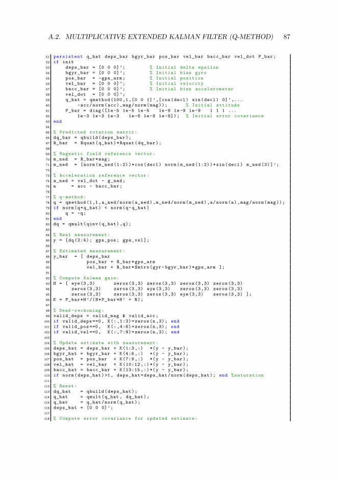
A.2. MULTIPLICATIVE EXTENDED KALMAN FILTER (Q-METHOD) 87
51 persistent q_hat deps_bar bgyr_bar pos_bar vel_bar bacc_bar vel_dot P_bar ;52 if init53 deps_bar = [0 0 0] ’; % Initial delta epsilon54 bgyr_bar = [0 0 0] ’; % Initial bias gyro55 pos_bar = -gps_arm ; % Initial position56 vel_bar = [0 0 0] ’; % Initial velocity57 bacc_bar = [0 0 0] ’; % Initial bias accelerometer58 vel_dot = [0 0 0] ’;59 q_hat = qmethod (100 ,1 ,[0 0 1]’,[ cos(decl) sin(decl) 0] ’ ,...60 -acc/norm(acc),mag/norm(mag)); % Initial attitude61 P_bar = diag ([1e -5 1e -5 1e -5 1e -9 1e -9 1e -9 1 1 1 ...62 1e -3 1e -3 1e -3 1e -8 1e -8 1e -8]); % Initial error covariance63 end64
65 % Predicted rotation matrix :66 dq_bar = qbuild ( deps_bar );67 R_bar = Rquat ( q_hat )* Rquat ( dq_bar );68
69 % Magnetic field reference vector :70 m_ned = R_bar *mag;71 m_ned = [norm( m_ned (1:2) )*cos(decl) norm( m_ned (1:2) )*sin(decl) m_ned (3) ]’;72
73 % Acceleration reference vector :74 a_ned = vel_dot - g_ned ;75 a = acc - bacc_bar ;76
77 % q- method :78 q = qmethod (1,1, a_ned /norm( a_ned ),m_ned /norm( m_ned ),a/norm(a),mag/norm(mag));79 if norm(q+ q_hat ) < norm(q- q_hat )80 q = -q;81 end82 dq = qmult (qinv( q_hat ),q);83
84 % Real measurement :85 y = [dq (2:4) ; gps_pos ; gps_vel ];86
87 % Estimated measurement :88 y_bar = [ deps_bar89 pos_bar + R_bar * gps_arm90 vel_bar + R_bar * Smtrx (gyr - bgyr_bar )* gps_arm ];91
92 % Compute Kalman gain:93 H = [ eye (3 ,3) zeros (3 ,3) zeros (3 ,3) zeros (3 ,3) zeros (3 ,3)94 zeros (3 ,3) zeros (3 ,3) eye (3 ,3) zeros (3 ,3) zeros (3 ,3)95 zeros (3 ,3) zeros (3 ,3) zeros (3 ,3) eye (3 ,3) zeros (3 ,3) ];96 K = P_bar *H ’/(H* P_bar *H’ + R);97
98 % Dead - reckoning :99 valid_deps = valid_mag & valid_acc ;
100 if valid_deps ==0 , K(: ,1:3)= zeros (n ,3); end101 if valid_pos ==0 , K(: ,4:6)= zeros (n ,3); end102 if valid_vel ==0 , K(: ,7:9)= zeros (n ,3); end103
104 % Update estimate with measurement :105 deps_hat = deps_bar + K(1:3 ,:) *(y - y_bar );106 bgyr_hat = bgyr_bar + K(4:6 ,:) *(y - y_bar );107 pos_hat = pos_bar + K(7:9 ,:) *(y - y_bar );108 vel_hat = vel_bar + K(10:12 ,:) *(y - y_bar );109 bacc_hat = bacc_bar + K(13:15 ,:) *(y - y_bar );110 if norm( deps_hat ) >1, deps_hat = deps_hat /norm( deps_hat ); end % saturation111
112 % Reset :113 dq_hat = qbuild ( deps_hat );114 q_hat = qmult (q_hat , dq_hat );115 q_hat = q_hat /norm( q_hat );116 deps_hat = [0 0 0] ’;117
118 % Compute error covariance for updated estimate :
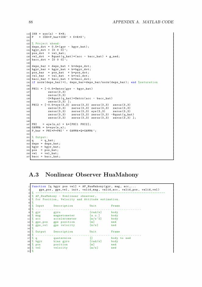
88 APPENDIX A. MATLAB CODE
119 IKH = eye(n) - K*H;120 P = IKH* P_bar *IKH ’ + K*R*K ’;121
122 % Project ahead :123 deps_dot = 0.5*( gyr - bgyr_hat );124 bgyr_dot = [0 0 0] ’;125 pos_dot = vel_hat ;126 vel_dot = Rquat ( q_hat )*( acc - bacc_hat ) + g_ned ;127 bacc_dot = [0 0 0] ’;128
129 deps_bar = deps_hat + h* deps_dot ;130 bgyr_bar = bgyr_hat + h* bgyr_dot ;131 pos_bar = pos_hat + h* pos_dot ;132 vel_bar = vel_hat + h* vel_dot ;133 bacc_bar = bacc_hat + h* bacc_dot ;134 if norm( deps_bar ) >1, deps_bar = deps_bar /norm( deps_bar ); end % saturation135
136 PHI1 = [ -0.5* Smtrx (gyr - bgyr_hat )137 zeros (3 ,3)138 zeros (3 ,3)139 -2* Rquat ( q_hat )* Smtrx (acc - bacc_hat )140 zeros (3 ,3) ];141 PHI2 = [ -0.5* eye (3 ,3) zeros (3 ,3) zeros (3 ,3) zeros (3 ,3)142 zeros (3 ,3) zeros (3 ,3) zeros (3 ,3) zeros (3 ,3)143 zeros (3 ,3) zeros (3 ,3) eye (3 ,3) zeros (3 ,3)144 zeros (3 ,3) zeros (3 ,3) zeros (3 ,3) -Rquat ( q_hat )145 zeros (3 ,3) zeros (3 ,3) zeros (3 ,3) zeros (3 ,3) ];146
147 PHI = eye(n,n) + h*[ PHI1 PHI2 ];148 GAMMA = h*eye(n,n);149 P_bar = PHI*P*PHI ’ + GAMMA *Q*GAMMA ’;150
151 % Output :152 q = q_hat ;153 deps = deps_hat ;154 bgyr = bgyr_hat ;155 pos = pos_hat ;156 vel = vel_hat ;157 bacc = bacc_hat ;
A.3 Nonlinear Observer HuaMahony
1 function [q bgyr pos vel] = AP_HuaMahony (gyr , mag , acc ,...2 gps_pos , gps_vel , init , valid_mag , valid_acc , valid_pos , valid_vel )3 % ------------------------------------------------------------------------4 % AP_HuaMahony - Nonlinear observer ,5 % for Position , Velocity and Attitude estimation .6 %7 % Input Description Unit Frame8 % ...........................................................9 % gyr gyro [rad/s] body
10 % mag magnetometer [a.u.] body11 % acc accelerometer [m/s^2] body12 % gps_pos gps position [m] ned13 % gps_vel gps velocity [m/s] ned14 %15 % Output Description Unit Frame16 % ...........................................................17 % q quaternion [] body to ned18 % bgyr bias gyro [rad/s] body19 % pos position [m] ned20 % vel velocity [m/s] ned21 %
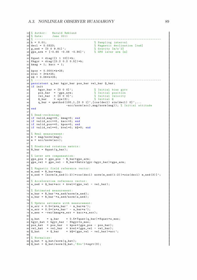
A.3. NONLINEAR OBSERVER HUAMAHONY 89
22 % Author : Harald Nøkland23 % Date: June 201124 % ------------------------------------------------------------------------25 h = 0.01; % Sampling interval26 decl = 0.0323; % Magnetic declination [rad]27 g_ned = [0 0 9.81] ’; % Gravity [m/s^2]28 gps_arm = [ -0.65 -0.08 -0.90] ’; % GPS lever arm [m]29
30 Kquat = diag ([1 1 10])*h;31 Kbgyr = diag ([0.2 0.2 0.5]) *h;32 kmag = 1; kacc = 1;33
34 kpos = 0.0001* h*25;35 kvel = 3*h*25;36 kQ = 0.06* h*25;37 % ------------------------------------------------------------------------38 persistent q_bar bgyr_bar pos_bar vel_bar Q_bar ;39 if init40 bgyr_bar = [0 0 0] ’; % Initial bias gyro41 pos_bar = -gps_arm ; % Initial position42 vel_bar = [0 0 0] ’; % Initial velocity43 Q_bar = eye (3); % Initial Q44 q_bar = qmethod (100 ,1 ,[0 0 1]’,[ cos(decl) sin(decl) 0] ’ ,...45 -acc/norm(acc),mag/norm(mag)); % Initial attitude46 end47
48 % Dead - reckoning :49 if valid_mag ==0 , kmag =0; end50 if valid_acc ==0 , kacc =0; end51 if valid_pos ==0 , kpos =0; end52 if valid_vel ==0 , kvel =0; kQ =0; end53
54 % Real measurement :55 m = mag/norm(mag);56 a = acc/norm(acc);57
58 % Predicted rotation matrix :59 R_bar = Rquat ( q_bar );60
61 % Lever arm compensation :62 gps_pos = gps_pos - R_bar * gps_arm ;63 gps_vel = gps_vel - R_bar * Smtrx (gyr - bgyr_bar )* gps_arm ;64
65 % Magnetic field reference vector :66 m_ned = R_bar *mag;67 m_ned = [norm( m_ned (1:2) )*cos(decl) norm( m_ned (1:2) )*sin(decl) m_ned (3) ]’;68
69 % Acceleration reference vector :70 a_ned = Q_bar *acc + kvel *( gps_vel - vel_bar );71
72 % Estimated measurement :73 m_bar = R_bar ’* m_ned /norm( m_ned );74 a_bar = R_bar ’* a_ned /norm( a_ned );75
76 % Update estimate with measurement :77 m_err = 0.5*( m*m_bar ’ - m_bar *m ’);78 a_err = 0.5*( a*a_bar ’ - a_bar *a ’);79 w_mes = -vex(kmag* m_err + kacc* a_err );80
81 q_hat = q_bar + 0.5* Tquat ( q_bar )* Kquat * w_mes ;82 bgyr_hat = bgyr_bar - Kbgyr * w_mes ;83 pos_hat = pos_bar + kpos *( gps_pos - pos_bar );84 vel_hat = vel_bar + kvel *( gps_vel - vel_bar );85 Q_hat = Q_bar + kQ *( gps_vel - vel_bar )*acc ’;86
87 % Normalize :88 q_hat = q_hat /norm( q_hat );89 Q_hat = Q_hat /norm(Q_hat ,’fro ’)*sqrt (3);
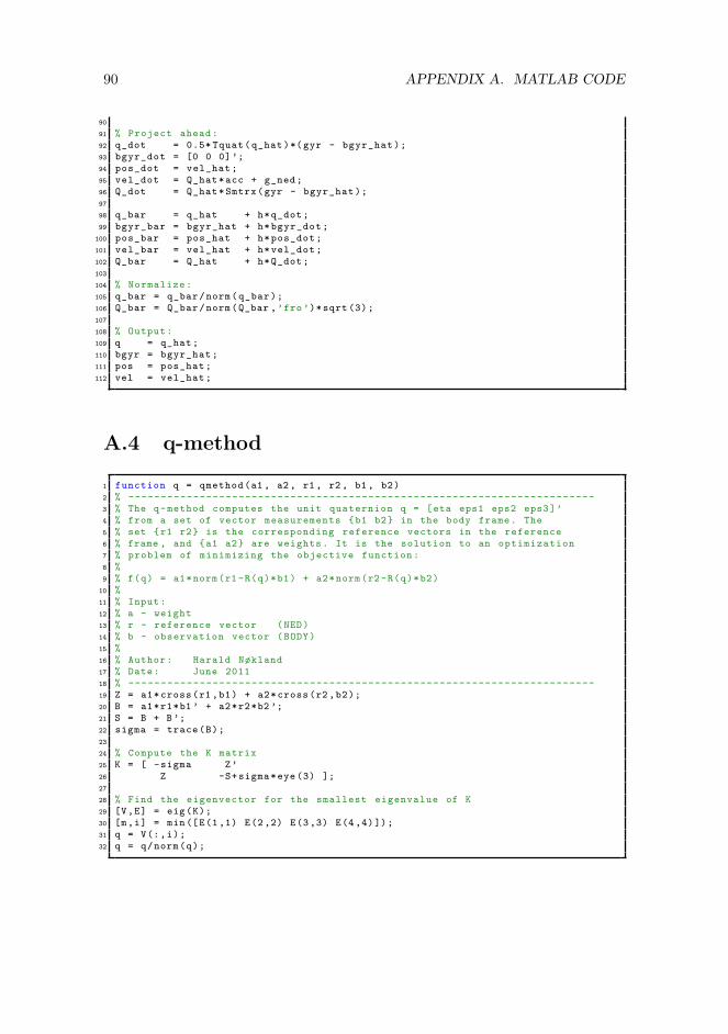
90 APPENDIX A. MATLAB CODE
90
91 % Project ahead :92 q_dot = 0.5* Tquat ( q_hat )*( gyr - bgyr_hat );93 bgyr_dot = [0 0 0] ’;94 pos_dot = vel_hat ;95 vel_dot = Q_hat *acc + g_ned ;96 Q_dot = Q_hat * Smtrx (gyr - bgyr_hat );97
98 q_bar = q_hat + h* q_dot ;99 bgyr_bar = bgyr_hat + h* bgyr_dot ;
100 pos_bar = pos_hat + h* pos_dot ;101 vel_bar = vel_hat + h* vel_dot ;102 Q_bar = Q_hat + h* Q_dot ;103
104 % Normalize :105 q_bar = q_bar /norm( q_bar );106 Q_bar = Q_bar /norm(Q_bar ,’fro ’)*sqrt (3);107
108 % Output :109 q = q_hat ;110 bgyr = bgyr_hat ;111 pos = pos_hat ;112 vel = vel_hat ;
A.4 q-method
1 function q = qmethod (a1 , a2 , r1 , r2 , b1 , b2)2 % ------------------------------------------------------------------------3 % The q- method computes the unit quaternion q = [eta eps1 eps2 eps3]’4 % from a set of vector measurements b1 b2 in the body frame . The5 % set r1 r2 is the corresponding reference vectors in the reference6 % frame , and a1 a2 are weights . It is the solution to an optimization7 % problem of minimizing the objective function :8 %9 % f(q) = a1*norm(r1 -R(q)*b1) + a2*norm(r2 -R(q)*b2)
10 %11 % Input :12 % a - weight13 % r - reference vector (NED)14 % b - observation vector (BODY)15 %16 % Author : Harald Nøkland17 % Date: June 201118 % ------------------------------------------------------------------------19 Z = a1* cross (r1 ,b1) + a2* cross (r2 ,b2);20 B = a1*r1*b1 ’ + a2*r2*b2 ’;21 S = B + B ’;22 sigma = trace (B);23
24 % Compute the K matrix25 K = [ -sigma Z’26 Z -S+ sigma *eye (3) ];27
28 % Find the eigenvector for the smallest eigenvalue of K29 [V,E] = eig(K);30 [m,i] = min ([E(1 ,1) E(2 ,2) E(3 ,3) E(4 ,4) ]);31 q = V(:,i);32 q = q/norm(q);
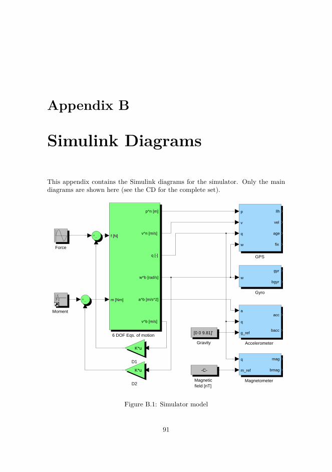
Appendix B
Simulink Diagrams
This appendix contains the Simulink diagrams for the simulator. Only the maindiagrams are shown here (see the CD for the complete set).
Moment
Magnetometer
q
m_ref
mag
bmag
Magneticfield [nT]
-C-
Gyro
w
gyr
bgyr
Gravity
[0 0 9.81]'
GPS
p
v
q
w
llh
vel
age
fixForce
D2
K*u
D1
K*uAccelerometer
a
q
g_ref
acc
bacc6 DOF Eqs. of motion
f [N]
m [Nm]
p^n [m]
v^n [m/s]
q [-]
w^b [rad/s]
a^b [m/s^2]
v^b [m/s]
Figure B.1: Simulator model
91
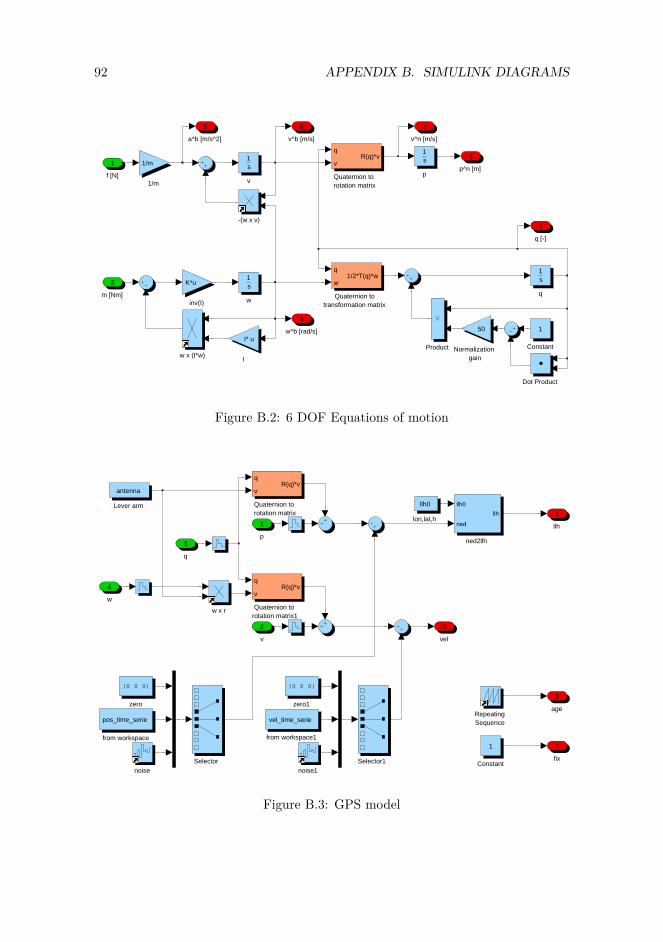
92 APPENDIX B. SIMULINK DIAGRAMS
v^b [m/s]
6
a^b [m/s^2]
5
w^b [rad/s]
4
q [-]
3
v^n [m/s]
2
p^n [m]
1
w x (I*w)
w
1s
v
1s
q
1s
p
1s
inv(I)
K*u
Quaternion to rotation matrix
q
vR(q)*v
Quaternion totransformation matrix
q
w1/2*T(q)*w
Product Normalizationgain
50
I
I* u
Dot Product
Constant
1
1/m
1/m
-(w x v)
m [Nm]
2
f [N]
1
Figure B.2: 6 DOF Equations of motion
fix
4
age
3
vel
2
llh
1
zero1
(0 0 0)
zero
(0 0 0)
w x r
noise1noise
ned2llh
llh0
ned
llhlon,lat,h
llh0
from workspace1
vel_time_serie
from workspace
pos_time_serie
Selector1Selector
RepeatingSequence
Quaternion to rotation matrix1
q
vR(q)*v
Quaternion to rotation matrix
q
vR(q)*v
Lever arm
antenna
Constant
1
w
4
q
3
v
2
p
1
Figure B.3: GPS model
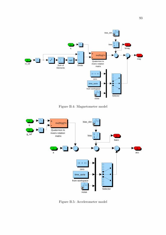
93
bmag
2
mag
1
zero
(0 0 0)
noise
from workspace
time_serie
bias_dot
bias1s
Sum ofElements
Selector
Quaternion toinvers rotation
matrix
q
vinv(R(q))*v
sqrtu2
Dividem_ref
2
q
1
Figure B.4: Magnetometer model
bacc
2
acc
1
zero
(0 0 0)
noise
from workspace
time_serie
bias_dot
bias1s
Selector
Quaternion toinvers rotation
matrix
q
vinv(R(q))*v
g_ref
3
q
2
a
1
Figure B.5: Accelerometer model
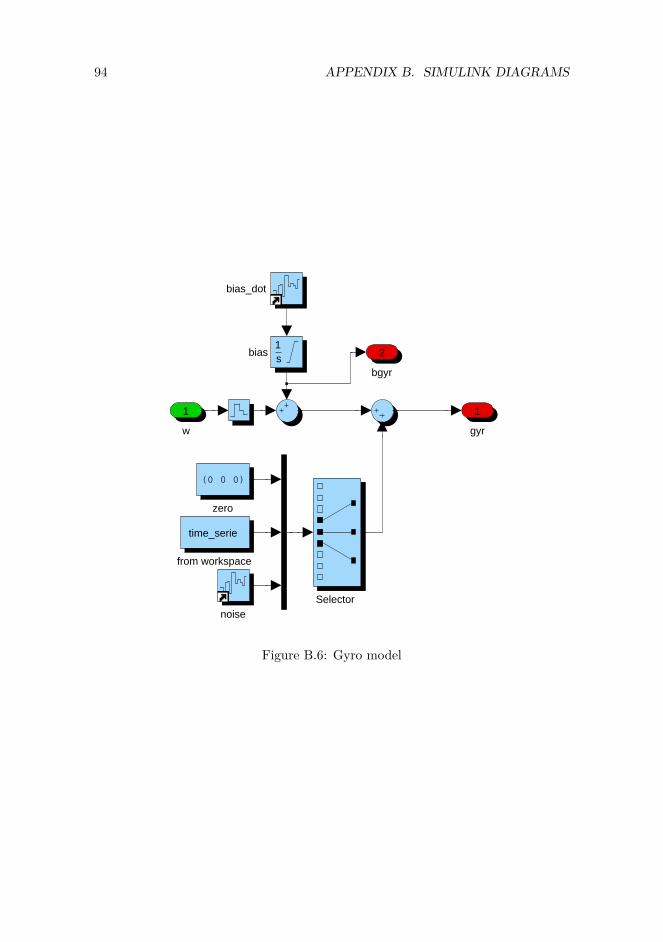
94 APPENDIX B. SIMULINK DIAGRAMS
bgyr
2
gyr
1
zero
(0 0 0)
noise
from workspace
time_serie
bias_dot
bias1s
Selector
w
1
Figure B.6: Gyro model

Appendix C
CD Content
All files needed to run the nonlinear observers developed in this thesis are includedon the CD. Some of the m-files are from the MSS GNC toolbox1, which is markedin the column named “T” for toolbox.
Table C.1: Matlab files included on CDFile T DescriptionA_EKF.m Attitude estimation, extended Kalman filterA_MEKF.m Attitude estimation, multiplicative extended
Kalman filterAP_HuaMahony.m Attitude, position and velocity estimation, non-
linear observer HuaMahonyAP_MEKF.m Attitude, position and velocity estimation, mul-
tiplicative extended Kalman filterAP_MEKF_qmethod.m Attitude, position and velocity estimation, mul-
tiplicative extended Kalman filter using q-method
dllh2dned.m Transformation from longitude, latitude andheight to NED coordinates
ecef2llh.m x Transformation from Cartesian to ellipsoidalECEF coordinates
euler2q.m x Transformation for Euler angles to quaternionllh2ecef.m x Transformation form ellipsoidal to Cartesian
ECEF coordinatesOmega.m Matrix in the quaternion differential equation
1MSS GNC is a Matlab toolbox for guidance, navigation and control. The toolbox is part ofthe Marine Systems Simulator (MSS). URL: <http://www.marinecontrol.org>
95
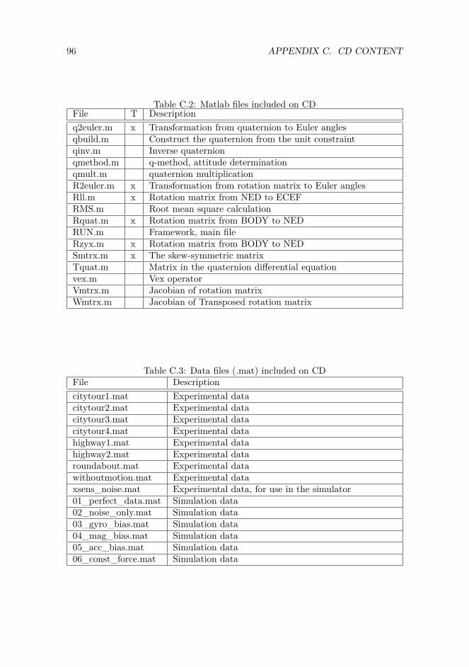
96 APPENDIX C. CD CONTENT
Table C.2: Matlab files included on CDFile T Descriptionq2euler.m x Transformation from quaternion to Euler anglesqbuild.m Construct the quaternion from the unit constraintqinv.m Inverse quaternionqmethod.m q-method, attitude determinationqmult.m quaternion multiplicationR2euler.m x Transformation from rotation matrix to Euler anglesRll.m x Rotation matrix from NED to ECEFRMS.m Root mean square calculationRquat.m x Rotation matrix from BODY to NEDRUN.m Framework, main fileRzyx.m x Rotation matrix from BODY to NEDSmtrx.m x The skew-symmetric matrixTquat.m Matrix in the quaternion differential equationvex.m Vex operatorVmtrx.m Jacobian of rotation matrixWmtrx.m Jacobian of Transposed rotation matrix
Table C.3: Data files (.mat) included on CDFile Descriptioncitytour1.mat Experimental datacitytour2.mat Experimental datacitytour3.mat Experimental datacitytour4.mat Experimental datahighway1.mat Experimental datahighway2.mat Experimental dataroundabout.mat Experimental datawithoutmotion.mat Experimental dataxsens_noise.mat Experimental data, for use in the simulator01_perfect_data.mat Simulation data02_noise_only.mat Simulation data03_gyro_bias.mat Simulation data04_mag_bias.mat Simulation data05_acc_bias.mat Simulation data06_const_force.mat Simulation data

97
Table C.4: Other files included on CDFile DescriptionextractPVT.c Decodes the MTB log files from Xsens
unitInstrument_Simulation_thesis.mdl Simulink simulatorMSc_Thesis_Nøkland(2011).pdf This Report