applied sciences

Article

Numerical–Experimental Correlation ofImpact-Induced Damages in CFRP Laminates

Andrea Sellitto 1,* , Salvatore Saputo 1, Francesco Di Caprio 2, Aniello Riccio 1 , Angela Russo 1

and Valerio Acanfora 1

1 Department of Engineering, University of Campania Luigi Vanvitelli, via Roma 29, 81031 Aversa, Italy;salvatore.saputo@unicampania.it (S.S.); aniello.riccio@unicampania.it (A.R.);angela.russo@unicampania.it (A.R.); valerio.acanfora@unicampania.it (V.A.)

2 C.I.R.A.—Italian Aerospace Research Centre, via Maiorise snc, 81043 Capua, Italy; f.dicaprio@cira.it* Correspondence: andrea.sellitto@unicampania.it; Tel.: +39-081-5010-407

Received: 8 April 2019; Accepted: 5 June 2019; Published: 11 June 2019�����������������

Featured Application: Numerical investigation on the damage behavior of CFRP laminatessubjected to low velocity impacts.

Abstract: Composite laminates are characterized by high mechanical in-plane properties and poorout-of-plane characteristics. This issue becomes even more relevant when dealing with impactphenomena occurring in the transverse direction. In aeronautics, Low Velocity Impacts (LVIs) mayoccur during the service life of the aircraft. LVI may produce damage inside the laminate, which arenot easily detectable and can seriously degrade the mechanical properties of the structure. In thispaper, a numerical-experimental investigation is carried out, in order to study the mechanical behaviorof rectangular laminated specimens subjected to low velocity impacts. The numerical model that bestrepresents the impact phenomenon has been chosen by numerical–analytical investigations. A userdefined material model (VUMAT) has been developed in Abaqus/Explicit environment to simulatethe composite intra-laminar damage behavior in solid elements. The analyses results were comparedto experimental test data on a laminated specimen, performed according to ASTM D7136 standard,in order to verify the robustness of the adopted numerical model and the influence of modelingparameters on the accuracy of numerical results.

Keywords: CFRP; Low Velocity Impacts; Cohesive Zone Model (CZM); Finite Element Analysis(FEA); VUMAT; inter-laminar damage; intra-laminar damage

1. Introduction

Composite materials are characterized by high mechanical properties values if compared to classicmetallic materials. However, their damage behavior is difficult to predict and control. As a matter offact, impact events on a composite structure are still a “hot topic” for research, nowadays. The differentimpact phenomena can be divided into three main groups, based on the velocity of the impactor:low velocity impacts, ballistic impacts, and hyper-velocity impacts. In particular, Low Velocity Impacts(LVIs) often result in Barely Visible Impact Damages (BVIDs), which can be hardly detected by the nakedeye, but may relevantly decrease the material strength [1–3]. Damages occurring as a consequenceof low velocity impacts include both intra-laminar (fiber and/or matrix failure) and inter-laminardamages (delaminations). Among the others, delaminations, which can growth under service loads,can seriously reduce the load carrying capability of the overall structure [4,5]. For this reason, a largenumber of studies, focused on the prediction of the damages (especially delaminations) induced by LVI,can be found in the literature. In these studies, different approaches, both analytical–numerical and

Appl. Sci. 2019, 9, 2372; doi:10.3390/app9112372 www.mdpi.com/journal/applsci

Appl. Sci. 2019, 9, 2372 2 of 21

experimental, were considered [6–9]. Different techniques are available and presented in the literature,able to predict and evaluate the damage and the residual strength during LVI phenomena. In [10],an acousto–ultrasonic approach was used to characterize the material impact strength. Low velocityanalytical impact prediction models available in the literature are often characterized by a large degreeof simplification. However, despite the simplifications in the models, good results can be achieved.In particular, the study in Reference [11] describes a numerical model for predicting the onset and thepropagation of damages arising from low velocity impacts induced by large and small impact masses.A further evolution of the analytical model for predicting the behavior of a thin-walled compositestructure during a low velocity-high mass impact phenomenon was presented in [12]. An additionalanalytical methodology based on the energy balance for the development of damage during a LVIphenomenon with the help of a localized strain field was introduced in [13]. However, analyticalapproaches, which can only be adopted for few particular conditions [1,6,7], cannot be generallyconsidered for a complete and detailed study of the impact event, due to inherent complexity of theimpact phenomenon itself [9,14–16]. A more comprehensive study of the impact phenomenon canbe surely obtained by means of numerical methods. Indeed, FEM (Finite Element Method) codescan be adopted to model a low velocity impact event on a composite specimen, taking into accountboth intra-laminar and inter-laminar damages [9,17–19]. In order to evaluate the intra-laminar andinter-laminar damage onset and propagation during an impact phenomenon, progressive damagemethods have been presented by several authors, showing good results compared to the experimentaldata. In [20], LVI tests were performed and the Puck criteria were adopted to analyze the compositestructure mechanical response. In the same work, an inter-laminar matrix crack density parameterwas introduced, in order to mitigate the computational cost, while decreasing, on the other side,the analysis accuracy. In [21–23], a model capable of predicting the inter-laminar damage in aunidirectional composite laminate was introduced. In particular, the proposed model took intoaccount a matrix non-linear shear behavior, focusing on the element characteristic length in order toalleviate the mesh dependency. Actually, fracture mechanic is widely used to model inter-laminardamage evolution through FE-based procedures such as Virtual Crack Closure Technique (VCCT) andCohesive Zone Model theory (CZM) [17,24–29]. In [29–31], the influence of intra-laminar damageson the inter-laminar ones is assessed adopting CZM, while, in [26,31–33], the mesh-dependencyissue of both inter-laminar and intra-laminar prediction models, which may lead to an unrealisticinter-laminar damage prediction, is emphasized. Low velocity impact events on composite specimens,with different stacking sequences, were studied in several works, which implement the intra-laminarand inter-laminar damages, respectively, by means of Continuum Damage Mechanics (CDM) andCZM approaches [9,18,19]. In these works, good results, in terms of correlation between numericaloutputs and experimental data, were obtained for various impact energy levels.

In this work, we propose an analytical model to preliminary evaluate the response of aunidirectional composite plate subjected to a low velocity impact. The analytical model has beendeveloped in accordance with [1,2,33]. Then, the results of the analytical model were compared withthose from a numerical model, which uses the analytical boundary conditions. Indeed, in the frame ofthis first step, the introduced analytical model, based on Classical Laminated Plate Theory (CLPT),was adopted as a benchmark for appropriately selecting the main numerical modeling parameters tobe used for the numerical procedure (element type, mesh density, element size, etc.). Subsequently, thenumerical model was improved, introducing the boundary conditions of the experimental test. Finally,a further numerical model, which takes into account inter-laminar and intra-laminar damages, wasimplemented and the results were compared with the experimental test ones. This final numerical testwas performed by adopting the numerical model, from the previous step, which best represents theimpact event. The low velocity impact phenomenon was numerically simulated by considering theboundary conditions and the specimen size according to the ASTM (American Society for Testing andMaterials) D7136 standard [34]. The composite specimens were subjected to a 10 J low velocity impact.A reduction of the computational time has been achieved by introducing global/local techniques [35]

Appl. Sci. 2019, 9, 2372 3 of 21

between the impacted area and the rest of the specimen. The results, in terms of intra-laminar andinter-laminar damages, have been compared with the experimental ones, obtained by means ofUltrasonic C-Scan tests. Further numerical–experimental correlations on the impactor displacementand velocity, the internal energy, and the force exerted during the impact have been performed as well.

Numerical results, obtained considering different Abaqus element types, were compared to eachother. The Finite Element Model has been discretized by means of SC8R Continuum shell elements andC3D8R Solid elements [36]. Inter-laminar damages were modeled by a Cohesive Zone Model basedapproach, while intra-laminar damage was modeled by means of Hashin’s failure criteria and gradualmaterial properties degradation rules. However, the intra-laminar damage model was only providedfor Continuum shell elements in Abaqus. Since no intra-laminar damage model was provided forSolid elements, a user-defined material model, able to take into account the intra-laminar damage,was implemented in a user subroutine VUMAT.

In Section 2, the theoretical background on the analytical model and on the intra-laminar damagemodel implemented in the VUMAT are presented. In Section 3, the test cases are introduced, while inSection 4 the results are presented and discussed.

2. Theoretical background

2.1. Classical Laminated Plate Theory

A multi-degree of freedom analytical model [1,2,37] was introduced in order to study the impactevent. A simply supported plate was analytically solved by using the Classical Laminated PlateTheory. The solutions for the analytical approach were obtained in terms of contact force, maximumdisplacement, impactor velocity, and kinetic energy. Then, a system of ordinary differential equations(ODE), representing the simply supported plate, coupled with a differential equation representing theimpactor motion, was obtained.

A laminated composite plate, with in-plane dimensions a and b, respectively, along the x- andy-directions, was considered. The plate was considered simply supported along the four edges,and a concentrated force was applied at the center (x0 = a/2, y0 = b/2). Under these assumptions,the equation of motion along the transverse direction can be expressed as the following system ofordinary differential equations [1]:

..αmn +ω2

mnαmn =4F

abI1sin

(mπx0

a

)sin

(nπy0

b

), (1)

In Equation (1), F is a concentrated applied force, while ωmn, which is the natural frequency of thesystem for the strain modes m,n, is given by:

ωmn =

√π4

a4I1(D11m4 + 2(D12 + 2D66)m2n2r2 − 4D16m3nr− 4D26mn3r3 + D22n4r4), (2)

where Dij are the terms of the bending stiffness matrix, I1 is the mass per unit length, and r = a/b.As reported in [1], when both values of m and n are negative, the effects of deflection in the plate

become negligible. The choice of high positive values for both values is related to the phenomenonbeing analyzed: as the values of m and n increase, the rotary inertia and shear deformation effectsbecomes significant.

Moreover, the following Equation (3), governing the impactor dynamic, has been considered:

M..z(t) + Fc(t) = 0, (3)

where M and..z(t) are, respectively, the impactor mass and acceleration, Fc(t) is the contact force, and t

is the time variable.

Appl. Sci. 2019, 9, 2372 4 of 21

A proper contact law has been chosen to couple Equations (3) and (1). In particular, the contactforce Fc(t) has been related to the indentation α = z(t) − w0(x0,y0,t), expressed as the difference betweenthe impactor displacement z(t) and the laminate central point displacement w0(x0,y0,t). In this work,a linearized form of the Hertz Contact Law was adopted [37], therefore the contact force history, exertedduring the impact phenomenon, can be expressed as:

Fc(t) = kyα, (4)

where ky represents the linearized contact stiffness.The boundary conditions of the system of ODEs are:

αmn(0) =.αmn(0) = 0, (5)

z(0) = 0.z(0) = V

(6)

where V is the initial velocity of the impactor.

2.2. Composites Damage Criteria

In order to account for the damage behavior of the laminate, a User Material was developed in theABAQUS FEM environment capable to consider the fiber and matrix damage mechanisms in tensionand compression [4,19,29]. Each failure mode consisted of two different phases. Initially, a linearmechanical behavior is considered up to the damage initiation threshold. Then, the damage evolutionup to the complete damage is evaluated.

The criteria used for evaluate the damage initiation are based on Hashin’s (fiber and matrix tensionand fiber compression) and Puck–Shurmann [38] (matrix compression) failure criteria, as reported inEquations (7)–(10).

F f t =(σ1

XT

)≥ 1 i f σ1 ≥ 0, (7)

F f c =

(σ1

XC

)≥ 1 i f σ1 < 0, (8)

Fmt =(σ2

YT

)2+

(τ12

S12

)2

+

(τ23

S23

)2

≥ 1 i f σ2 ≥ 0, (9)

Fmc =

τnt

SA23 − µntσnn

2

+

(τnl

S12 − µnlσn

)2

≥ 1 i f σ2 < 0, (10)

where XT and XC are the fiber tensile and compressive strengths, YT is the matrix tensile strength, andS12 and S23 are respectively the longitudinal and transverse shear strengths. Moreover, the parametersintroduced in Equation (10) have been defined with respect to the potential fracture plane; in particular,SA

23 is the transverse shear strength in the potential fracture plane, µnt and µnl are respectively thefriction coefficients in the transverse and longitudinal directions, σnn is the normal stress, and τnt andτnl are respectively the shear stresses in the transverse and longitudinal directions. Indeed, experimentshave demonstrated that unidirectional laminates experience shear fail [39] when subjected to transversecompressive loads, with a fracture plane oriented with an angle θf = 53◦ ± 2◦ [21]. Hence, to correctlyevaluate the damage status of the laminate, the stress/strain components in the θf oriented fractureplane have been considered, instead of the nominal 0◦ oriented nominal plane.

Appl. Sci. 2019, 9, 2372 5 of 21

Therefore, the stress components in the general fracture plane L-N-T oriented with a fractureangle θf, as in Figure 1, can be obtained as a function of the stress components defined in the laminacoordinate system 1-2-3:

σn = σ2 cos2 θ f + σ3 sin2 θ f + 2τ23 cosθ f sinθ fτnl = τ23 cosθ f + τ31 cosθ f

τnt = (σ3 − σ2) cosθ f sinθ f + τ23(cos2 θ f − sin2 θ f

) . (11)

Appl. Sci. 2019, 9, x 5 of 22

( ) ( )

σ σ θ σ θ τ θ θτ τ θ τ θ

τ σ σ θ θ τ θ θ

= + + = +

= − + −

2 22 3 23

23 31

2 23 2 23

cos sin 2 cos sincos cos

cos sin cos sin

n f f f f

nl f f

nt f f f f

. (11)

Figure 1. Compressive matrix failure and fracture plane.

Hence, the parameters related to the fracture angle introduced in Equation (10) can be defined [40]:

φ θ= ⋅ − °2 90f , (12)

μ φ= tannt , (13)

( )φφ

−=23

1 sin2 cos

CA YS , (14)

μ μ= ⋅ 12

23nl nt A

SS

, (15)

where YT is the matrix compressive strength. Each mode is characterized by the failure behavior reported in Figure 2. In particular, a linear

elastic behavior with an initial stiffness K can be observed up to location A, which identifies the damage onset. Then, each location B on the segment AC identifies a partial damage condition characterized by a degraded stiffness Kd, up to location C, where the complete failure can be observed.

1

3

2

L

T

NσTNσNN

σLN

θf

Figure 1. Compressive matrix failure and fracture plane.

Hence, the parameters related to the fracture angle introduced in Equation (10) can be defined [40]:

φ = 2 · θ f − 90◦, (12)

µnt = tanφ, (13)

SA23 =

YC(1− sinφ)2 cosφ

, (14)

µnl = µnt ·S12

SA23

, (15)

where YT is the matrix compressive strength.Each mode is characterized by the failure behavior reported in Figure 2. In particular, a linear

elastic behavior with an initial stiffness K can be observed up to location A, which identifies the damageonset. Then, each location B on the segment AC identifies a partial damage condition characterized bya degraded stiffness Kd, up to location C, where the complete failure can be observed.

Appl. Sci. 2019, 9, 2372 6 of 21Appl. Sci. 2019, 9, x 6 of 22

Figure 2. Constitutive relation adopted for fiber and matrix failure modes in tension and

compression.

To take into account the material stiffness degradations in locations B, the damage coefficients di [36] are introduced for each failure mode:

( )( ) ( )

δ δ δδ δ δ

δ δ δ

−= ≤ ≤ ∈

−

0, , , 0

, , ,0, , ,

; ; , , ,ti eq i eq i eq t

i i eq i eq i eqti eq i eq i eq

d i fc ft mc mt . (16)

Indeed, the damaged stiffness matrix CD can be expressed as a function of the damage coefficients as:

( ) ( )( )( )( ) ( )

( )

ν

ν

− − − = − − − −

1 21 1

12 2 2

12

1 1 1 01 1 1 1 0

0 0 1

f f m

f m m

s

d E d d E

d d E d ED

D d GDC , (17)

where D = 1 – (1 – df)(1 – dm)ν12ν21, and df, dm, and ds are respectively the fiber, matrix, and shear damage coefficients:

( )( )( )( )

σσ

σσ

≥= < ≥= <

= − − − − −

11

11

22

22

ˆif 0ˆif 0

ˆif 0ˆif 0

1 1 1 1 1

ftf

fc

mtm

mc

s ft fc mt mc

dd

d

dd

d

d d d d d

. (18)

However, this methodology has been found strongly dependent on the domain discretization. Hence, to reduce mesh dependencies, the element characteristic length LC has been introduced. In this work, the solution proposed by Bazant and Oh [39] and reported in Equation (19) has been adopted:

θ=

cosip

C

AL , (19)

where Aip is the Area of the element corresponding to the ip-th integration point and θ is the fracture angle. Then, the equivalent displacements was computed as a function of the element characteristic length LC:

( ) ( ) ( )ε γ γδ

⋅ + ⋅ + ⋅=

2 2 2

2 12 230,

C C Cmt eq

mt

L L L

F, (20)

δeq

σeq

O

A

B

C

KKd

Gc

δteqδ0eq

σ0eq

Figure 2. Constitutive relation adopted for fiber and matrix failure modes in tension and compression.

To take into account the material stiffness degradations in locations B, the damage coefficientsdi [36] are introduced for each failure mode:

di =δt

i,eq

(δi,eq − δ

0i,eq

)δi,eq

(δt

i,eq − δ0i,eq

) ; δ0i,eq ≤ δi,eq ≤ δ

ti,eq; i ∈ ( f c, f t, mc, mt). (16)

Indeed, the damaged stiffness matrix CD can be expressed as a function of the damagecoefficients as:

CD =1D

(1− d f

)E1

(1− d f

)(1− dm)ν21E1 0(

1− d f)(1− dm)ν12E2 (1− dm)E2 0

0 0 D(1− ds)G12

, (17)

where D = 1 − (1 − df)(1 − dm)ν12ν21, and df, dm, and ds are respectively the fiber, matrix, and sheardamage coefficients:

d f =

{d f t if σ̂11 ≥ 0d f c if σ̂11 < 0

dm =

{dmt if σ̂22 ≥ 0dmc if σ̂22 < 0

ds = 1−(1− d f t

)(1− d f c

)(1− dmt)(1− dmc)

(18)

However, this methodology has been found strongly dependent on the domain discretization.Hence, to reduce mesh dependencies, the element characteristic length LC has been introduced. In thiswork, the solution proposed by Bazant and Oh [39] and reported in Equation (19) has been adopted:

LC =

√Aip

cosθ, (19)

where Aip is the Area of the element corresponding to the ip-th integration point and θ is the fractureangle. Then, the equivalent displacements was computed as a function of the element characteristiclength LC:

δ0mt,eq =

√(ε2 · LC)

2 + (γ12 · LC)2 + (γ23 · LC)

2

√Fmt

, (20)

δ0mc,eq =

√(γln · LC)

2 + (γtn · LC)2

√Fmc

, (21)

δ0i,eq =

√(ε1 · LC)

2

√Fi

; i ∈ ( f c, f t), (22)

Appl. Sci. 2019, 9, 2372 7 of 21

δtf t,eq =

2GTIC

σ0f t,eq

, (23)

δtf c,eq =

2GCIC

σ0f c,eq

, (24)

δtmt,eq =

2GTIIC

σ0mt,eq

, (25)

δtmc,eq =

2GCIIC

σ0mc,eq

, (26)

where GTIC and GC

IC are the tensile and compressive Mode I fracture toughness, GTIIC and GC

IIC arethe tensile and compressive Mode II fracture toughness, and:

γnt = γ12 cosθ f + γ13 sinθ f , (27)

γnl = −ε2 cosθ f sinθ f + ε3 cosθ f sinθ f + γ23(2 cos2 θ f − 1

). (28)

3. Test Cases Descriptions

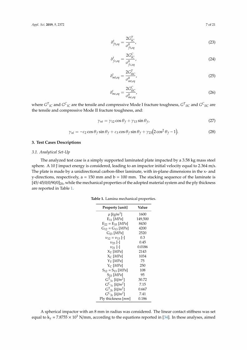
3.1. Analytical Set-Up

The analyzed test case is a simply supported laminated plate impacted by a 3.58 kg mass steelsphere. A 10 J impact energy is considered, leading to an impactor initial velocity equal to 2.364 m/s.The plate is made by a unidirectional carbon-fiber laminate, with in-plane dimensions in the x- andy-directions, respectively, a = 150 mm and b = 100 mm. The stacking sequence of the laminate is[45/-45/0/0/90/0]2S, while the mechanical properties of the adopted material system and the ply thicknessare reported in Table 1.

Table 1. Lamina mechanical properties.

Property [unit] Value

ρ [kg/m3] 1600E11 [MPa] 149,500

E22 = E33 [MPa] 8430G12 = G13 [MPa] 4200

G23 [MPa] 2520υ12 = υ13 [-] 0.3

υ23 [-] 0.45υ21 [-] 0.0186

XT [MPa] 2143XC [MPa] 1034YT [MPa] 75YC [MPa] 250

S12 = S13 [MPa] 108S23 [MPa] 95

GT1c [kJ/m2] 30.72

GC1c [kJ/m2] 7.15

GT2c [kJ/m2] 0.667

GC2c [kJ/m2] 7.41

Ply thickness [mm] 0.186

A spherical impactor with an 8 mm in radius was considered. The linear contact stiffness was setequal to ky = 7.8755 × 103 N/mm, according to the equations reported in [34]. In these analyses, aimed

Appl. Sci. 2019, 9, 2372 8 of 21

to preliminary assess the elastic behavior of the structure under impact loading conditions, only theelastic behavior has been taken into account. Therefore, no damage has been considered.

3.2. Experimental Set-Up

The experimental impact test was performed according to the ASTM D7136 standard [34], as shownin Figure 3.

Appl. Sci. 2019, 9, x 8 of 22

YC [MPa] 250 S12 = S13 [MPa] 108

S23 [MPa] 95 GT1c [kJ/m2] 30.72 GC1c [kJ/m2] 7.15 GT2c [kJ/m2] 0.667 GC2c [kJ/m2] 7.41

Ply thickness [mm] 0.186

A spherical impactor with an 8 mm in radius was considered. The linear contact stiffness was set equal to ky = 7.8755 ×∙103 N/mm, according to the equations reported in [34]. In these analyses, aimed to preliminary assess the elastic behavior of the structure under impact loading conditions, only the elastic behavior has been taken into account. Therefore, no damage has been considered.

3.2. Experimental Set-Up

The experimental impact test was performed according to the ASTM D7136 standard [34], as shown in Figure 3.

Figure 3. Experimental set-up.

The three tested specimens were cut from a single CFRP plate by using the waterjet technique. The CFRP plate is composed of prepreg high modulus carbon fiber and thermoset epoxy resin, cured in autoclave. The test was performed with the CEAST Fractovis plus drop tower test machine. The plates were normally impacted at the center. The impactor was a 16 mm diameter hemisphere made of hardened steel, with a mass of 3.58 kg. A 10 J impact energy was considered. Ultrasonic inspections were performed on the specimen prior to the impact test to assure the lack of manufacturing defects, and after the experimental test to evaluate the damaged area.

4. Results and Discussion

4.1. Preliminary Analyses

The analytical approach results expressed in terms of impactor displacement, contact force, impactor velocity, and kinetic energy versus time are shown respectively in Figures 4–7. The results were obtained by considering an increasing number of modes.

Figure 3. Experimental set-up.

The three tested specimens were cut from a single CFRP plate by using the waterjet technique.The CFRP plate is composed of prepreg high modulus carbon fiber and thermoset epoxy resin, cured inautoclave. The test was performed with the CEAST Fractovis plus drop tower test machine. The plateswere normally impacted at the center. The impactor was a 16 mm diameter hemisphere made ofhardened steel, with a mass of 3.58 kg. A 10 J impact energy was considered. Ultrasonic inspectionswere performed on the specimen prior to the impact test to assure the lack of manufacturing defects,and after the experimental test to evaluate the damaged area.

4. Results and Discussion

4.1. Preliminary Analyses

The analytical approach results expressed in terms of impactor displacement, contact force,impactor velocity, and kinetic energy versus time are shown respectively in Figures 4–7. The resultswere obtained by considering an increasing number of modes.Appl. Sci. 2019, 9, x 9 of 22

Figure 4. Analytical solution—impactor displacement.

Figure 5. Analytical solution—contact force history.

Figure 6. Analytical solution—impactor velocity.

-4-3-2-101234

0 1 2 3 4 5

Impa

ctor

Disp

lace

men

t [m

m]

Time [ms]

Impactor Displacement

m,n =2 m,n =3 m,n =5 m,n =6 m,n =10

010002000300040005000600070008000

0 1 2 3 4 5

Forc

e [N

]

Time [ms]

Contact Force History

m,n =2m,n =3m,n =5m,n =6m,n =10

-3

-2

-1

0

1

2

3

0 1 2 3 4 5

Velo

city

[m/s

]

Time [ms]

Impactor Velocity

m,n =2 m,n =3 m,n =5 m,n =6 m,n =10

Figure 4. Analytical solution—impactor displacement.

Appl. Sci. 2019, 9, 2372 9 of 21

Appl. Sci. 2019, 9, x 9 of 22

Figure 4. Analytical solution—impactor displacement.

Figure 5. Analytical solution—contact force history.

Figure 6. Analytical solution—impactor velocity.

-4-3-2-101234

0 1 2 3 4 5

Impa

ctor

Disp

lace

men

t [m

m]

Time [ms]

Impactor Displacement

m,n =2 m,n =3 m,n =5 m,n =6 m,n =10

010002000300040005000600070008000

0 1 2 3 4 5

Forc

e [N

]

Time [ms]

Contact Force History

m,n =2m,n =3m,n =5m,n =6m,n =10

-3

-2

-1

0

1

2

3

0 1 2 3 4 5

Velo

city

[m/s

]

Time [ms]

Impactor Velocity

m,n =2 m,n =3 m,n =5 m,n =6 m,n =10

Figure 5. Analytical solution—contact force history.

Appl. Sci. 2019, 9, x 9 of 22

Figure 4. Analytical solution—impactor displacement.

Figure 5. Analytical solution—contact force history.

Figure 6. Analytical solution—impactor velocity.

-4-3-2-101234

0 1 2 3 4 5

Impa

ctor

Disp

lace

men

t [m

m]

Time [ms]

Impactor Displacement

m,n =2 m,n =3 m,n =5 m,n =6 m,n =10

010002000300040005000600070008000

0 1 2 3 4 5

Forc

e [N

]

Time [ms]

Contact Force History

m,n =2m,n =3m,n =5m,n =6m,n =10

-3

-2

-1

0

1

2

3

0 1 2 3 4 5

Velo

city

[m/s

]

Time [ms]

Impactor Velocity

m,n =2 m,n =3 m,n =5 m,n =6 m,n =10

Figure 6. Analytical solution—impactor velocity.Appl. Sci. 2019, 9, x 10 of 22

Figure 7. Analytical solution—kinetic energy.

Figures 4 and 5 highlight that lower values of m and n results in higher values of stiffness. Indeed, increasing the m and n values led to a decrease of the peak force and to an increase in the maximum deflection of the plate central point. Additionally, according to Figures 4 and 5, the panel response in terms of impact force and maximum deflection tended to converge as the values of m and n increased. Figure 6 shows the trends of the impact velocity considering different m and n values. Although the velocity had the same initial and final values, different m and n led to different velocity trends. Moreover, as a direct consequence of the variation of the impact velocity, the kinetic energy, shown in Figure 7, showed different behavior when low values of m and n were considered. However, as m and n increase, the graphs shown in Figures 4–7 appear to be perfectly overlapped.

Then, the numerical results were compared with the analytical ones. The m,n = 10 analytical results were chosen as the reference analytical solution.

In order to define the numerical model which best-fit the analytical results, several parameters were investigated, such as the element type (reduced integration continuum shell elements SC8R and reduced integration solid elements C3D8R), the in-plane element size (1 mm, 2 mm, and 4 mm), and the number of elements along the thickness direction. In particular, Continuum Shell elements were discretized with 1, 12, and 24 elements in the thickness direction, while Solid elements were discretized with 24 elements in the thickness direction (one element per ply). Hence, more than one orientation is associated to the continuum shell elements belonging to the models characterized by less than 24 elements in the thickness direction.

In the numerical analyses, the plate was considered simply supported on the edges, as reported in Figure 8. In the framework of preliminary analyses, aimed to compare the analytical model with the numerical ones to determine the numerical parameters which best represent the mechanical behavior of the plate subjected to low velocity impact, both the inter-laminar and intra-laminar damages were neglected.

Figure 8. Shell model boundary conditions.

0

2

4

6

8

10

12

0 1 2 3 4 5

Ener

gy [J

]

Time [ms]

Kinetic Energy

m,n =2m,n =3m,n =5m,n =6m,n =10

Figure 7. Analytical solution—kinetic energy.

Figures 4 and 5 highlight that lower values of m and n results in higher values of stiffness. Indeed,increasing the m and n values led to a decrease of the peak force and to an increase in the maximumdeflection of the plate central point. Additionally, according to Figures 4 and 5, the panel response interms of impact force and maximum deflection tended to converge as the values of m and n increased.Figure 6 shows the trends of the impact velocity considering different m and n values. Althoughthe velocity had the same initial and final values, different m and n led to different velocity trends.Moreover, as a direct consequence of the variation of the impact velocity, the kinetic energy, shown inFigure 7, showed different behavior when low values of m and n were considered. However, as m andn increase, the graphs shown in Figures 4–7 appear to be perfectly overlapped.

Appl. Sci. 2019, 9, 2372 10 of 21

Then, the numerical results were compared with the analytical ones. The m,n = 10 analyticalresults were chosen as the reference analytical solution.

In order to define the numerical model which best-fit the analytical results, several parameterswere investigated, such as the element type (reduced integration continuum shell elements SC8Rand reduced integration solid elements C3D8R), the in-plane element size (1 mm, 2 mm, and 4 mm),and the number of elements along the thickness direction. In particular, Continuum Shell elementswere discretized with 1, 12, and 24 elements in the thickness direction, while Solid elements werediscretized with 24 elements in the thickness direction (one element per ply). Hence, more than oneorientation is associated to the continuum shell elements belonging to the models characterized by lessthan 24 elements in the thickness direction.

In the numerical analyses, the plate was considered simply supported on the edges, as reported inFigure 8. In the framework of preliminary analyses, aimed to compare the analytical model with thenumerical ones to determine the numerical parameters which best represent the mechanical behaviorof the plate subjected to low velocity impact, both the inter-laminar and intra-laminar damageswere neglected.

Appl. Sci. 2019, 9, x 10 of 22

Figure 7. Analytical solution—kinetic energy.

Figures 4 and 5 highlight that lower values of m and n results in higher values of stiffness. Indeed, increasing the m and n values led to a decrease of the peak force and to an increase in the maximum deflection of the plate central point. Additionally, according to Figures 4 and 5, the panel response in terms of impact force and maximum deflection tended to converge as the values of m and n increased. Figure 6 shows the trends of the impact velocity considering different m and n values. Although the velocity had the same initial and final values, different m and n led to different velocity trends. Moreover, as a direct consequence of the variation of the impact velocity, the kinetic energy, shown in Figure 7, showed different behavior when low values of m and n were considered. However, as m and n increase, the graphs shown in Figures 4–7 appear to be perfectly overlapped.

Then, the numerical results were compared with the analytical ones. The m,n = 10 analytical results were chosen as the reference analytical solution.

In order to define the numerical model which best-fit the analytical results, several parameters were investigated, such as the element type (reduced integration continuum shell elements SC8R and reduced integration solid elements C3D8R), the in-plane element size (1 mm, 2 mm, and 4 mm), and the number of elements along the thickness direction. In particular, Continuum Shell elements were discretized with 1, 12, and 24 elements in the thickness direction, while Solid elements were discretized with 24 elements in the thickness direction (one element per ply). Hence, more than one orientation is associated to the continuum shell elements belonging to the models characterized by less than 24 elements in the thickness direction.

In the numerical analyses, the plate was considered simply supported on the edges, as reported in Figure 8. In the framework of preliminary analyses, aimed to compare the analytical model with the numerical ones to determine the numerical parameters which best represent the mechanical behavior of the plate subjected to low velocity impact, both the inter-laminar and intra-laminar damages were neglected.

Figure 8. Shell model boundary conditions.

0

2

4

6

8

10

12

0 1 2 3 4 5

Ener

gy [J

]

Time [ms]

Kinetic Energy

m,n =2m,n =3m,n =5m,n =6m,n =10

Figure 8. Shell model boundary conditions.

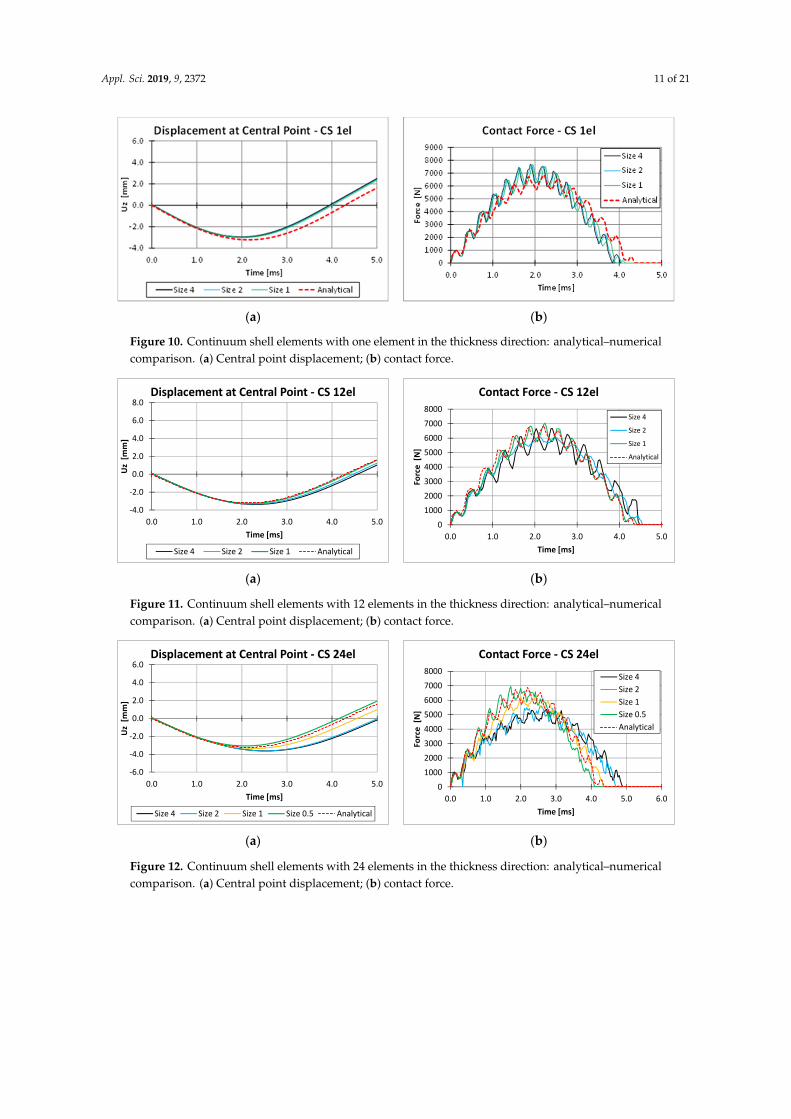
In Figures 9–13, the numerical and analytical results, in terms of displacement of the impactorand contact force, are compared. In particular, the results shown in Figure 9 were obtained by usinga shell element formulation, while the results in Figures 10–12 were obtained by using a continuumshell formulation considering, respectively, 1, 12, and 24 elements in the thickness direction. Finally,in Figure 13, the results obtained by using a solid element formulation, with 24 elements in the thicknessdirection, are introduced.

Appl. Sci. 2019, 9, x 11 of 22

In Figures 9–13, the numerical and analytical results, in terms of displacement of the impactor and contact force, are compared. In particular, the results shown in Figure 9 were obtained by using a shell element formulation, while the results in Figures 10–12 were obtained by using a continuum shell formulation considering, respectively, 1, 12, and 24 elements in the thickness direction. Finally, in Figure 13, the results obtained by using a solid element formulation, with 24 elements in the thickness direction, are introduced.

(a) (b)

Figure 9. Shell elements: analytical–numerical comparison. (a) Central point displacement; (b) contact force.

(a) (b)

Figure 10. Continuum shell elements with one element in the thickness direction: analytical–numerical comparison. (a) Central point displacement; (b) contact force.

(a) (b)

Figure 11. Continuum shell elements with 12 elements in the thickness direction: analytical–numerical comparison. (a) Central point displacement; (b) contact force.

-4.0

-2.0

0.0

2.0

4.0

6.0

0.0 1.0 2.0 3.0 4.0 5.0

Uz [

mm

]

Time [ms]

Displacement at Central Point - Shell

Size 4 Size 2 Size 1 Analytical

0100020003000400050006000700080009000

0.0 1.0 2.0 3.0 4.0 5.0

Forc

e [N

]

Time [ms]

Contact Force - ShellSize 4Size 2Size 1Analytical

-4.0

-2.0

0.0

2.0

4.0

6.0

8.0

0.0 1.0 2.0 3.0 4.0 5.0

Uz [

mm

]

Time [ms]

Displacement at Central Point - CS 12el

Size 4 Size 2 Size 1 Analytical

010002000300040005000600070008000

0.0 1.0 2.0 3.0 4.0 5.0

Forc

e [N

]

Time [ms]

Contact Force - CS 12el

Size 4

Size 2

Size 1

Analytical

Figure 9. Shell elements: analytical–numerical comparison. (a) Central point displacement;(b) contact force.

Appl. Sci. 2019, 9, 2372 11 of 21

Appl. Sci. 2019, 9, x 11 of 22

In Figures 9–13, the numerical and analytical results, in terms of displacement of the impactor and contact force, are compared. In particular, the results shown in Figure 9 were obtained by using a shell element formulation, while the results in Figures 10–12 were obtained by using a continuum shell formulation considering, respectively, 1, 12, and 24 elements in the thickness direction. Finally, in Figure 13, the results obtained by using a solid element formulation, with 24 elements in the thickness direction, are introduced.

(a) (b)

Figure 9. Shell elements: analytical–numerical comparison. (a) Central point displacement; (b) contact force.

(a) (b)

Figure 10. Continuum shell elements with one element in the thickness direction: analytical–numerical comparison. (a) Central point displacement; (b) contact force.

(a) (b)

Figure 11. Continuum shell elements with 12 elements in the thickness direction: analytical–numerical comparison. (a) Central point displacement; (b) contact force.

-4.0

-2.0

0.0

2.0

4.0

6.0

0.0 1.0 2.0 3.0 4.0 5.0

Uz [

mm

]

Time [ms]

Displacement at Central Point - Shell

Size 4 Size 2 Size 1 Analytical

0100020003000400050006000700080009000

0.0 1.0 2.0 3.0 4.0 5.0

Forc

e [N

]

Time [ms]

Contact Force - ShellSize 4Size 2Size 1Analytical

-4.0

-2.0

0.0

2.0

4.0

6.0

8.0

0.0 1.0 2.0 3.0 4.0 5.0

Uz [

mm

]

Time [ms]

Displacement at Central Point - CS 12el

Size 4 Size 2 Size 1 Analytical

010002000300040005000600070008000

0.0 1.0 2.0 3.0 4.0 5.0

Forc

e [N

]

Time [ms]

Contact Force - CS 12el

Size 4

Size 2

Size 1

Analytical

Figure 10. Continuum shell elements with one element in the thickness direction: analytical–numericalcomparison. (a) Central point displacement; (b) contact force.

Appl. Sci. 2019, 9, x 11 of 22

In Figures 9–13, the numerical and analytical results, in terms of displacement of the impactor and contact force, are compared. In particular, the results shown in Figure 9 were obtained by using a shell element formulation, while the results in Figures 10–12 were obtained by using a continuum shell formulation considering, respectively, 1, 12, and 24 elements in the thickness direction. Finally, in Figure 13, the results obtained by using a solid element formulation, with 24 elements in the thickness direction, are introduced.

(a) (b)

Figure 9. Shell elements: analytical–numerical comparison. (a) Central point displacement; (b) contact force.

(a) (b)

Figure 10. Continuum shell elements with one element in the thickness direction: analytical–numerical comparison. (a) Central point displacement; (b) contact force.

(a) (b)

Figure 11. Continuum shell elements with 12 elements in the thickness direction: analytical–numerical comparison. (a) Central point displacement; (b) contact force.

-4.0

-2.0

0.0

2.0

4.0

6.0

0.0 1.0 2.0 3.0 4.0 5.0

Uz [

mm

]

Time [ms]

Displacement at Central Point - Shell

Size 4 Size 2 Size 1 Analytical

0100020003000400050006000700080009000

0.0 1.0 2.0 3.0 4.0 5.0

Forc

e [N

]

Time [ms]

Contact Force - ShellSize 4Size 2Size 1Analytical

-4.0

-2.0

0.0

2.0

4.0

6.0

8.0

0.0 1.0 2.0 3.0 4.0 5.0

Uz [

mm

]

Time [ms]

Displacement at Central Point - CS 12el

Size 4 Size 2 Size 1 Analytical

010002000300040005000600070008000

0.0 1.0 2.0 3.0 4.0 5.0

Forc

e [N

]

Time [ms]

Contact Force - CS 12el

Size 4

Size 2

Size 1

Analytical

Figure 11. Continuum shell elements with 12 elements in the thickness direction: analytical–numericalcomparison. (a) Central point displacement; (b) contact force.

Appl. Sci. 2019, 9, x 12 of 22

(a) (b)

Figure 12. Continuum shell elements with 24 elements in the thickness direction: analytical–numerical comparison. (a) Central point displacement; (b) contact force.

(a) (b)

Figure 13. Solid elements with 24 elements in the thickness direction: analytical–numerical comparison. (a) Central point displacement; (b) contact force.

According to the Figures 9–13, Shell and Solid elements’ models were not particularly influenced by the in-plane element size. On the other hand, Continuum shell elements’ models were more sensitive to the in-plane element size as the number of elements in the thickness direction increased. In particular, the numerical results of the Continuum shell model with 12 and 24 elements in the thickness direction associated to coarser mesh (size 2 mm or 4 mm) differed noticeably from the analytical results. This is mainly due to hourglass problems, which can be relevant for the reduced integration scheme elements. Unfortunately, the reduced integration scheme is mandatory in Abaqus/Explicit when Continuum shell elements were adopted. To alleviate hourglass deformation problems that could arise in the numerical models, the default hourglass controls available in Abaqus /Explicit [36] was adopted.

In general, the results highlight that the best results were obtained by the Solid element model discretized with one element per ply and an in-plane element size equal to 1 mm; however, a good numerical–analytical correlation was obtained also by the Continuum shell mode, discretized by 12 elements in the thickness direction and an in-plane element size equal to 1 mm. Indeed, this last configuration was chosen for the analysis presented hereafter due to its excellent compromise between low computational cost and agreement with the analytical solution.

Despite their simplifications, the analytical models available in the literature well describe the behavior of a CFRP plate subjected to impact loading conditions. Hence, the numerical model was validated by comparisons with the analytical one, and the used modeling approach, neglecting in this preliminary phase the damages, has been assessed. Once the accuracy of the impact numerical model is verified, some considerations should be made about the relevant difference between the

-6.0

-4.0

-2.0

0.0

2.0

4.0

6.0

0.0 1.0 2.0 3.0 4.0 5.0

Uz [

mm

]

Time [ms]

Displacement at Central Point - CS 24el

Size 4 Size 2 Size 1 Size 0.5 Analytical

010002000300040005000600070008000

0.0 1.0 2.0 3.0 4.0 5.0 6.0

Forc

e [N

]

Time [ms]

Contact Force - CS 24elSize 4Size 2Size 1Size 0.5Analytical

-4.0

-2.0

0.0

2.0

4.0

6.0

0.0 1.0 2.0 3.0 4.0 5.0

Uz [

mm

]

Time [ms]

Displacement at Central Point - SD 24el

Size 4 Size 2 Size 1 Analytical

010002000300040005000600070008000

0.0 1.0 2.0 3.0 4.0 5.0

Forc

e [N

]

Time [ms]

Contact Force - SD 24elSize 4Size 2Size 1Analytical

Figure 12. Continuum shell elements with 24 elements in the thickness direction: analytical–numericalcomparison. (a) Central point displacement; (b) contact force.

Appl. Sci. 2019, 9, 2372 12 of 21

Appl. Sci. 2019, 9, x 12 of 22

(a) (b)

Figure 12. Continuum shell elements with 24 elements in the thickness direction: analytical–numerical comparison. (a) Central point displacement; (b) contact force.

(a) (b)

Figure 13. Solid elements with 24 elements in the thickness direction: analytical–numerical comparison. (a) Central point displacement; (b) contact force.

According to the Figures 9–13, Shell and Solid elements’ models were not particularly influenced by the in-plane element size. On the other hand, Continuum shell elements’ models were more sensitive to the in-plane element size as the number of elements in the thickness direction increased. In particular, the numerical results of the Continuum shell model with 12 and 24 elements in the thickness direction associated to coarser mesh (size 2 mm or 4 mm) differed noticeably from the analytical results. This is mainly due to hourglass problems, which can be relevant for the reduced integration scheme elements. Unfortunately, the reduced integration scheme is mandatory in Abaqus/Explicit when Continuum shell elements were adopted. To alleviate hourglass deformation problems that could arise in the numerical models, the default hourglass controls available in Abaqus /Explicit [36] was adopted.

In general, the results highlight that the best results were obtained by the Solid element model discretized with one element per ply and an in-plane element size equal to 1 mm; however, a good numerical–analytical correlation was obtained also by the Continuum shell mode, discretized by 12 elements in the thickness direction and an in-plane element size equal to 1 mm. Indeed, this last configuration was chosen for the analysis presented hereafter due to its excellent compromise between low computational cost and agreement with the analytical solution.

Despite their simplifications, the analytical models available in the literature well describe the behavior of a CFRP plate subjected to impact loading conditions. Hence, the numerical model was validated by comparisons with the analytical one, and the used modeling approach, neglecting in this preliminary phase the damages, has been assessed. Once the accuracy of the impact numerical model is verified, some considerations should be made about the relevant difference between the

-6.0

-4.0

-2.0

0.0

2.0

4.0

6.0

0.0 1.0 2.0 3.0 4.0 5.0

Uz [

mm

]

Time [ms]

Displacement at Central Point - CS 24el

Size 4 Size 2 Size 1 Size 0.5 Analytical

010002000300040005000600070008000

0.0 1.0 2.0 3.0 4.0 5.0 6.0

Forc

e [N

]

Time [ms]

Contact Force - CS 24elSize 4Size 2Size 1Size 0.5Analytical

-4.0

-2.0

0.0

2.0

4.0

6.0

0.0 1.0 2.0 3.0 4.0 5.0

Uz [

mm

]

Time [ms]

Displacement at Central Point - SD 24el

Size 4 Size 2 Size 1 Analytical

010002000300040005000600070008000

0.0 1.0 2.0 3.0 4.0 5.0

Forc

e [N

]

Time [ms]

Contact Force - SD 24elSize 4Size 2Size 1Analytical

Figure 13. Solid elements with 24 elements in the thickness direction: analytical–numerical comparison.(a) Central point displacement; (b) contact force.

According to the Figures 9–13, Shell and Solid elements’ models were not particularly influencedby the in-plane element size. On the other hand, Continuum shell elements’ models were more sensitiveto the in-plane element size as the number of elements in the thickness direction increased. In particular,the numerical results of the Continuum shell model with 12 and 24 elements in the thickness directionassociated to coarser mesh (size 2 mm or 4 mm) differed noticeably from the analytical results. This ismainly due to hourglass problems, which can be relevant for the reduced integration scheme elements.Unfortunately, the reduced integration scheme is mandatory in Abaqus/Explicit when Continuumshell elements were adopted. To alleviate hourglass deformation problems that could arise in thenumerical models, the default hourglass controls available in Abaqus/Explicit [36] was adopted.

In general, the results highlight that the best results were obtained by the Solid element modeldiscretized with one element per ply and an in-plane element size equal to 1 mm; however, a goodnumerical–analytical correlation was obtained also by the Continuum shell mode, discretized by12 elements in the thickness direction and an in-plane element size equal to 1 mm. Indeed, this lastconfiguration was chosen for the analysis presented hereafter due to its excellent compromise betweenlow computational cost and agreement with the analytical solution.

Despite their simplifications, the analytical models available in the literature well describe thebehavior of a CFRP plate subjected to impact loading conditions. Hence, the numerical model wasvalidated by comparisons with the analytical one, and the used modeling approach, neglecting in thispreliminary phase the damages, has been assessed. Once the accuracy of the impact numerical modelis verified, some considerations should be made about the relevant difference between the boundaryconditions implemented in the analytical model and the ones implemented in the experimentaltest. Actually, simply supported conditions have been considered in the analytical and preliminarynumerical models; however, the boundary conditions of the experimental test, suggested by the ASTMstandards and reported in Figure 14, are substantially different. These boundary conditions are aconsequence of a support fixture whose degrees of freedom are restrained and four rigid clamps,also modeled as rigid bodies, which hold the specimen still during impact and avoid any rebound.

Appl. Sci. 2019, 9, x 13 of 22

boundary conditions implemented in the analytical model and the ones implemented in the experimental test. Actually, simply supported conditions have been considered in the analytical and preliminary numerical models; however, the boundary conditions of the experimental test, suggested by the ASTM standards and reported in Figure 14, are substantially different. These boundary conditions are a consequence of a support fixture whose degrees of freedom are restrained and four rigid clamps, also modeled as rigid bodies, which hold the specimen still during impact and avoid any rebound.

(a) (b)

Figure 14. Boundary conditions. (a) Analytical; (b) experimental.

A further numerical model obtained with the implementation of the Experimental boundary condition (BC-E) was introduced to understand the effects of boundary conditions on the numerical results. In Figure 15, the analytical, experimental and numerical results of the shell model obtained by considering both analytical (BC-A) and experimental (BC-E) boundary conditions were compared.

Figure 15. Contact force comparison between analytical and numerical boundary conditions.

In Figure 15, a comparison between experimental, analytical, and numerical results, in terms of force as a function of the time, is reported. The comparison shows that in the first part of the curve both numerical and analytical models were in agreement with the experimental results. However, after a first phase, the analytical model and the FEM BC-A numerical model greatly differed from the experimental result. On the other hand, the FEM BC-E numerical model was characterized by the same mechanical response in terms of stiffness of the laminate, up to the maximum force peak. Indeed, neglecting the damages in the numerical model resulted in grater force peak, if compared with the experiment. Once the accuracy of the numerical model, in terms of elastic response, was established, the numerical models which provided the best results compared to the analytical solution was considered for the final impact test: final Continuum shell model and Final 3D solid model. Since Abaqus does not provide any intra-laminar damage models for Solid elements, a VUMAT was introduced. On the other side, Abaqus built-in Hashin’s criteria were used for model discretized by means of Continuum shell elements. For both the final continuum shell model and the final solid FEM model, gradual material properties degradation rules have been adopted for intra-laminar damage progression and inter-laminar damage were implemented through cohesive elements layers placed at plies interfaces.

0

1000

2000

3000

4000

5000

6000

7000

8000

9000

10000

0 1 2 3 4 5 6

Forc

e [N

]

Time [ms]

Contact Force

Experimental

Analytical

FEM BC-E

FEM BC-A

Figure 14. Boundary conditions. (a) Analytical; (b) experimental.

Appl. Sci. 2019, 9, 2372 13 of 21

A further numerical model obtained with the implementation of the Experimental boundarycondition (BC-E) was introduced to understand the effects of boundary conditions on the numericalresults. In Figure 15, the analytical, experimental and numerical results of the shell model obtained byconsidering both analytical (BC-A) and experimental (BC-E) boundary conditions were compared.

Appl. Sci. 2019, 9, x 13 of 22

boundary conditions implemented in the analytical model and the ones implemented in the experimental test. Actually, simply supported conditions have been considered in the analytical and preliminary numerical models; however, the boundary conditions of the experimental test, suggested by the ASTM standards and reported in Figure 14, are substantially different. These boundary conditions are a consequence of a support fixture whose degrees of freedom are restrained and four rigid clamps, also modeled as rigid bodies, which hold the specimen still during impact and avoid any rebound.

(a) (b)

Figure 14. Boundary conditions. (a) Analytical; (b) experimental.

A further numerical model obtained with the implementation of the Experimental boundary condition (BC-E) was introduced to understand the effects of boundary conditions on the numerical results. In Figure 15, the analytical, experimental and numerical results of the shell model obtained by considering both analytical (BC-A) and experimental (BC-E) boundary conditions were compared.

Figure 15. Contact force comparison between analytical and numerical boundary conditions.

In Figure 15, a comparison between experimental, analytical, and numerical results, in terms of force as a function of the time, is reported. The comparison shows that in the first part of the curve both numerical and analytical models were in agreement with the experimental results. However, after a first phase, the analytical model and the FEM BC-A numerical model greatly differed from the experimental result. On the other hand, the FEM BC-E numerical model was characterized by the same mechanical response in terms of stiffness of the laminate, up to the maximum force peak. Indeed, neglecting the damages in the numerical model resulted in grater force peak, if compared with the experiment. Once the accuracy of the numerical model, in terms of elastic response, was established, the numerical models which provided the best results compared to the analytical solution was considered for the final impact test: final Continuum shell model and Final 3D solid model. Since Abaqus does not provide any intra-laminar damage models for Solid elements, a VUMAT was introduced. On the other side, Abaqus built-in Hashin’s criteria were used for model discretized by means of Continuum shell elements. For both the final continuum shell model and the final solid FEM model, gradual material properties degradation rules have been adopted for intra-laminar damage progression and inter-laminar damage were implemented through cohesive elements layers placed at plies interfaces.

0

1000

2000

3000

4000

5000

6000

7000

8000

9000

10000

0 1 2 3 4 5 6

Forc

e [N

]

Time [ms]

Contact Force

Experimental

Analytical

FEM BC-E

FEM BC-A

Figure 15. Contact force comparison between analytical and numerical boundary conditions.

In Figure 15, a comparison between experimental, analytical, and numerical results, in terms offorce as a function of the time, is reported. The comparison shows that in the first part of the curveboth numerical and analytical models were in agreement with the experimental results. However,after a first phase, the analytical model and the FEM BC-A numerical model greatly differed fromthe experimental result. On the other hand, the FEM BC-E numerical model was characterized bythe same mechanical response in terms of stiffness of the laminate, up to the maximum force peak.Indeed, neglecting the damages in the numerical model resulted in grater force peak, if comparedwith the experiment. Once the accuracy of the numerical model, in terms of elastic response, wasestablished, the numerical models which provided the best results compared to the analytical solutionwas considered for the final impact test: final Continuum shell model and Final 3D solid model.Since Abaqus does not provide any intra-laminar damage models for Solid elements, a VUMAT wasintroduced. On the other side, Abaqus built-in Hashin’s criteria were used for model discretized bymeans of Continuum shell elements. For both the final continuum shell model and the final solid FEMmodel, gradual material properties degradation rules have been adopted for intra-laminar damageprogression and inter-laminar damage were implemented through cohesive elements layers placed atplies interfaces.

4.2. Final Solid Model

This Final Solid model was created by introducing two different meshed areas connect by aglobal–local conditions. Indeed, in the specimen impacted area, where most of the damage is supposedto develop (Figure 16) a ply-by-ply refined discretization was considered with each ply represented by asingle layer of 3D solid elements C3D8R with a reduced integration scheme. On the contrary, the externalglobal domain has been modeled with a coarser continuum shell mesh. With this discretization scheme,an accurate study can be performed by reducing, at the same time, the computational effort [40].

Appl. Sci. 2019, 9, 2372 14 of 21

Appl. Sci. 2019, 9, x 14 of 22

4.2. Final Solid Model

This Final Solid model was created by introducing two different meshed areas connect by a global–local conditions. Indeed, in the specimen impacted area, where most of the damage is supposed to develop (Figure 16) a ply-by-ply refined discretization was considered with each ply represented by a single layer of 3D solid elements C3D8R with a reduced integration scheme. On the contrary, the external global domain has been modeled with a coarser continuum shell mesh. With this discretization scheme, an accurate study can be performed by reducing, at the same time, the computational effort [40].

Figure 16. Domain and boundary conditions.

For 3D solid elements, the intra-laminar damage model introduced in Section 2.2 was applied by means of a VUMAT. Moreover, since the inter-laminar damages are likely to occur only between plies with different fiber orientation, zero-thickness cohesive layers were placed only in these locations. As highlighted in Figure 17, cohesive layers were connected to the adjacent layer by means of tie-constraint. Table 2 reports the mechanical properties of the cohesive material system, which were experimentally evaluated by means of three-point bending (En, Et, Es), double cantilever beam (Nmax, GIc), and end notched flexure tests (Tmax and Smax, GIIc and GIIIc).

Figure 17. Exploded model (detail).

Table 2. Cohesive mechanical properties.

Property [unit] Value En [MPa/mm] 1.155∙× 106 Et [MPa/mm] 6∙× 105 Es [MPa/mm] 6∙× 105 Nmax [MPa] 62.3 Tmax [MPa] 92.3 Smax [MPa] 92.3

Figure 16. Domain and boundary conditions.

For 3D solid elements, the intra-laminar damage model introduced in Section 2.2 was appliedby means of a VUMAT. Moreover, since the inter-laminar damages are likely to occur only betweenplies with different fiber orientation, zero-thickness cohesive layers were placed only in these locations.As highlighted in Figure 17, cohesive layers were connected to the adjacent layer by means oftie-constraint. Table 2 reports the mechanical properties of the cohesive material system, which wereexperimentally evaluated by means of three-point bending (En, Et, Es), double cantilever beam (Nmax,GIc), and end notched flexure tests (Tmax and Smax, GIIc and GIIIc).

Appl. Sci. 2019, 9, x 14 of 22

4.2. Final Solid Model

This Final Solid model was created by introducing two different meshed areas connect by a global–local conditions. Indeed, in the specimen impacted area, where most of the damage is supposed to develop (Figure 16) a ply-by-ply refined discretization was considered with each ply represented by a single layer of 3D solid elements C3D8R with a reduced integration scheme. On the contrary, the external global domain has been modeled with a coarser continuum shell mesh. With this discretization scheme, an accurate study can be performed by reducing, at the same time, the computational effort [40].

Figure 16. Domain and boundary conditions.

For 3D solid elements, the intra-laminar damage model introduced in Section 2.2 was applied by means of a VUMAT. Moreover, since the inter-laminar damages are likely to occur only between plies with different fiber orientation, zero-thickness cohesive layers were placed only in these locations. As highlighted in Figure 17, cohesive layers were connected to the adjacent layer by means of tie-constraint. Table 2 reports the mechanical properties of the cohesive material system, which were experimentally evaluated by means of three-point bending (En, Et, Es), double cantilever beam (Nmax, GIc), and end notched flexure tests (Tmax and Smax, GIIc and GIIIc).

Figure 17. Exploded model (detail).

Table 2. Cohesive mechanical properties.

Property [unit] Value En [MPa/mm] 1.155∙× 106 Et [MPa/mm] 6∙× 105 Es [MPa/mm] 6∙× 105 Nmax [MPa] 62.3 Tmax [MPa] 92.3 Smax [MPa] 92.3

Figure 17. Exploded model (detail).

Table 2. Cohesive mechanical properties.

Property [unit] Value

En [MPa/mm] 1.155 × 106

Et [MPa/mm] 6 × 105

Es [MPa/mm] 6 × 105

Nmax [MPa] 62.3Tmax [MPa] 92.3Smax [MPa] 92.3GIc [kJ/m2] 0.18GIIc [kJ/m2] 0.5GIIIc [kJ/m2] 0.5

Both solid and cohesive elements have been discretized by 1× 1 mm2 elements. The external globaldomain, which has been modeled by one layer of Continuum shell SC8R elements along thicknessdirection, has been discretized with an element in-plane size of 4 mm. The specimen is constrainedby a fixture and four clamps, modeled with R3D4 rigid elements. The impactor was modeled as asphere of 16 mm diameter modeled with 3D Solid C3D8R elements. A surface-to-surface contact wasused between the impactor and the specimen. During the analysis, the completely damaged elementswere removed from the model to increase the computational efficiency. In particular, when cohesive

Appl. Sci. 2019, 9, 2372 15 of 21

elements were removed, plies can touch each other at the interfaces. Hence, a general contact on thewhole model was defined (except for the already defined impact surfaces) to take into account thisbehavior. A friction coefficient with a value of 0.5 was introduced for both impactor-to-ply contact andply-to-ply contact. Enhanced hourglass control was set to decrease hourglass problems related to thereduced integrated elements.

4.3. Final Continuum Shell Model

In the Final Continuum shell model, 12 continuum shell elements along thickness direction wereused to model the specimen (Figure 18). For each element, a composite layup composed of two plieswas defined.

Appl. Sci. 2019, 9, x 15 of 22

GIc [kJ/m2] 0.18 GIIc [kJ/m2] 0.5 GIIIc [kJ/m2] 0.5

Both solid and cohesive elements have been discretized by 1 × 1 mm2 elements. The external global domain, which has been modeled by one layer of Continuum shell SC8R elements along thickness direction, has been discretized with an element in-plane size of 4 mm. The specimen is constrained by a fixture and four clamps, modeled with R3D4 rigid elements. The impactor was modeled as a sphere of 16 mm diameter modeled with 3D Solid C3D8R elements. A surface-to-surface contact was used between the impactor and the specimen. During the analysis, the completely damaged elements were removed from the model to increase the computational efficiency. In particular, when cohesive elements were removed, plies can touch each other at the interfaces. Hence, a general contact on the whole model was defined (except for the already defined impact surfaces) to take into account this behavior. A friction coefficient with a value of 0.5 was introduced for both impactor-to-ply contact and ply-to-ply contact. Enhanced hourglass control was set to decrease hourglass problems related to the reduced integrated elements.

4.3. Final Continuum Shell Model

In the Final Continuum shell model, 12 continuum shell elements along thickness direction were used to model the specimen (Figure 18). For each element, a composite layup composed of two plies was defined.

Figure 18. Continuum shell elements domain.

The intra-laminar damages have been accounted by means of Hashin’s failure criteria, while cohesive layers placed at plies interfaces and introduced in Table 2 were used to model inter-laminar damage. The contact laws introduced in Section 4.2 were adopted.

4.4. Numerical–Experimental Correlation

In this section, a comparison between the experimental results and the numerical ones for the both investigated configurations (continuum shell element and solid elements) is performed considering both intra-laminar and inter-laminar damages. Three 10 J impact experimental tests were performed. The damaged area was acquired by means of the ultrasonic C-Scan. Figure 19 shows the C-scan of one representative specimen.

Figure 18. Continuum shell elements domain.

The intra-laminar damages have been accounted by means of Hashin’s failure criteria, whilecohesive layers placed at plies interfaces and introduced in Table 2 were used to model inter-laminardamage. The contact laws introduced in Section 4.2 were adopted.

4.4. Numerical–Experimental Correlation

In this section, a comparison between the experimental results and the numerical ones for the bothinvestigated configurations (continuum shell element and solid elements) is performed consideringboth intra-laminar and inter-laminar damages. Three 10 J impact experimental tests were performed.The damaged area was acquired by means of the ultrasonic C-Scan. Figure 19 shows the C-scan of onerepresentative specimen.Appl. Sci. 2019, 9, x 16 of 22

Figure 19. C-scan of the damaged area.

A linear pattern obtained by means of Abaqus/Viewer was used to evaluate the experimental damaged area. The tested specimens were comparable in terms of force, displacement, and kinetic energy as a function of the time, and inter-laminar damages. In particular, the experimental damaged area was about 250 mm2, while the numerical damaged area, evaluated by using different numerical models, was in the range 166–609 mm2.

The continuum shell model uses a lower number of interfaces between the plies, if compared with the solid element discretization model, and two plies with different orientations are discretized with only one element through the thickness. This assumption could influence the plate mechanical response, leading to different results in terms of delaminated area.

In Figures 20 and 21, the numerical results of the final Continuum shell model in terms of inter-laminar and intra-laminar damages are respectively reported.

Figure 20. Shell element model: delamination.

Figure 21. Shell element model: intra-laminar damages (envelope).

According to Figure 20, the simulation over predicts the size of the delamination. This over-prediction can be related to the shell formulation, which is not able to correctly predict the forces acting in the out-of-plane direction, and to the discretization in the thickness direction. Indeed,

Figure 19. C-scan of the damaged area.

A linear pattern obtained by means of Abaqus/Viewer was used to evaluate the experimentaldamaged area. The tested specimens were comparable in terms of force, displacement, and kineticenergy as a function of the time, and inter-laminar damages. In particular, the experimental damagedarea was about 250 mm2, while the numerical damaged area, evaluated by using different numericalmodels, was in the range 166–609 mm2.

Appl. Sci. 2019, 9, 2372 16 of 21

The continuum shell model uses a lower number of interfaces between the plies, if comparedwith the solid element discretization model, and two plies with different orientations are discretizedwith only one element through the thickness. This assumption could influence the plate mechanicalresponse, leading to different results in terms of delaminated area.

In Figures 20 and 21, the numerical results of the final Continuum shell model in terms ofinter-laminar and intra-laminar damages are respectively reported.

Appl. Sci. 2019, 9, x 16 of 22

Figure 19. C-scan of the damaged area.

A linear pattern obtained by means of Abaqus/Viewer was used to evaluate the experimental damaged area. The tested specimens were comparable in terms of force, displacement, and kinetic energy as a function of the time, and inter-laminar damages. In particular, the experimental damaged area was about 250 mm2, while the numerical damaged area, evaluated by using different numerical models, was in the range 166–609 mm2.

The continuum shell model uses a lower number of interfaces between the plies, if compared with the solid element discretization model, and two plies with different orientations are discretized with only one element through the thickness. This assumption could influence the plate mechanical response, leading to different results in terms of delaminated area.

In Figures 20 and 21, the numerical results of the final Continuum shell model in terms of inter-laminar and intra-laminar damages are respectively reported.

Figure 20. Shell element model: delamination.

Figure 21. Shell element model: intra-laminar damages (envelope).

According to Figure 20, the simulation over predicts the size of the delamination. This over-prediction can be related to the shell formulation, which is not able to correctly predict the forces acting in the out-of-plane direction, and to the discretization in the thickness direction. Indeed,

Figure 20. Shell element model: delamination.

Appl. Sci. 2019, 9, x 16 of 22

Figure 19. C-scan of the damaged area.

A linear pattern obtained by means of Abaqus/Viewer was used to evaluate the experimental damaged area. The tested specimens were comparable in terms of force, displacement, and kinetic energy as a function of the time, and inter-laminar damages. In particular, the experimental damaged area was about 250 mm2, while the numerical damaged area, evaluated by using different numerical models, was in the range 166–609 mm2.

The continuum shell model uses a lower number of interfaces between the plies, if compared with the solid element discretization model, and two plies with different orientations are discretized with only one element through the thickness. This assumption could influence the plate mechanical response, leading to different results in terms of delaminated area.

In Figures 20 and 21, the numerical results of the final Continuum shell model in terms of inter-laminar and intra-laminar damages are respectively reported.

Figure 20. Shell element model: delamination.

Figure 21. Shell element model: intra-laminar damages (envelope).

According to Figure 20, the simulation over predicts the size of the delamination. This over-prediction can be related to the shell formulation, which is not able to correctly predict the forces acting in the out-of-plane direction, and to the discretization in the thickness direction. Indeed,

Figure 21. Shell element model: intra-laminar damages (envelope).

According to Figure 20, the simulation over predicts the size of the delamination.This over-prediction can be related to the shell formulation, which is not able to correctly predictthe forces acting in the out-of-plane direction, and to the discretization in the thickness direction.Indeed, assuming 12 elements in the thickness direction reduces the number of interfaces where thedelamination can occur, leading to larger inter-laminar damages in the remaining interfaces.

Figures 22 and 23 show the predicted and measured contact force, impactor displacement,internal energy, and impactor velocity as a function of the time.

Appl. Sci. 2019, 9, x 17 of 22

assuming 12 elements in the thickness direction reduces the number of interfaces where the delamination can occur, leading to larger inter-laminar damages in the remaining interfaces.

Figures 22 and 23 show the predicted and measured contact force, impactor displacement, internal energy, and impactor velocity as a function of the time.

(a) (b)

Figure 22. Shell element model. (a) Contact force history; (b) impactor displacement.

(a) (b)

Figure 23. Shell element model. (a) Internal energy; (b) impactor velocity.

According to Figure 22a, the numerical curve deviates from the experimental one at about 0.3 ms due to anticipated numerical prediction of the onset of delaminations, resulting in a longer contact duration. This effect can be due to the lower number of interfaces. Moreover, the numerically overestimated impactor displacement (6.77% as reported in Figure 22b) and the underestimated residual internal energy of the numerical model (−28.52% as reported in Figure 23a), confirm the over-prediction of damages observed in the simulation. Hence, in the adopted numerical model, significant differences can be observed between the numerical and experimental inter-laminar and intra-laminar damages, as shown in Figures 20 and 21. In particular, the stiffness of the continuum shell element is underestimated if compared with experimental results. Indeed, the maximum displacement of the numerical result is lower than the experimental result in conjunction with a lower peak force.

The numerical results of the solid element model in terms of inter-laminar and intra-laminar damages are reported in Figures 24–27.

0

1000

2000

3000

4000

5000

6000

7000

8000

0 0.5 1 1.5 2 2.5 3 3.5 4 4.5

Forc

e [N

]

Time [ms]

Force History

Experimental

FEM 12el CS BC-E

-4

-3

-2

-1

0

1

2

0 0.5 1 1.5 2 2.5 3 3.5 4 4.5

Impa

ctor

Disp

lace

men

t [m

m]

Time [ms]

Impactor Displacement

Experimental

FEM 12el CS BC-E

0

2

4

6

8

10

12

0 0.5 1 1.5 2 2.5 3 3.5 4 4.5

Inte

rnal

Ene

rgy

[J]

Time [ms]

Internal Energy

Experimental

FEM 12el CS BC-E

-3

-2.5

-2

-1.5

-1

-0.5

0

0.5

1

1.5

2

2.5

0 0.5 1 1.5 2 2.5 3 3.5 4 4.5

Velo

city

[m/s

]

Time [ms]

Impactor Velocity

Experimental

FEM 12el CS BC-E

Figure 22. Shell element model. (a) Contact force history; (b) impactor displacement.

Appl. Sci. 2019, 9, 2372 17 of 21

Appl. Sci. 2019, 9, x 17 of 22

assuming 12 elements in the thickness direction reduces the number of interfaces where the delamination can occur, leading to larger inter-laminar damages in the remaining interfaces.

Figures 22 and 23 show the predicted and measured contact force, impactor displacement, internal energy, and impactor velocity as a function of the time.

(a) (b)

Figure 22. Shell element model. (a) Contact force history; (b) impactor displacement.

(a) (b)

Figure 23. Shell element model. (a) Internal energy; (b) impactor velocity.

According to Figure 22a, the numerical curve deviates from the experimental one at about 0.3 ms due to anticipated numerical prediction of the onset of delaminations, resulting in a longer contact duration. This effect can be due to the lower number of interfaces. Moreover, the numerically overestimated impactor displacement (6.77% as reported in Figure 22b) and the underestimated residual internal energy of the numerical model (−28.52% as reported in Figure 23a), confirm the over-prediction of damages observed in the simulation. Hence, in the adopted numerical model, significant differences can be observed between the numerical and experimental inter-laminar and intra-laminar damages, as shown in Figures 20 and 21. In particular, the stiffness of the continuum shell element is underestimated if compared with experimental results. Indeed, the maximum displacement of the numerical result is lower than the experimental result in conjunction with a lower peak force.

The numerical results of the solid element model in terms of inter-laminar and intra-laminar damages are reported in Figures 24–27.

0

1000

2000

3000

4000

5000

6000

7000

8000

0 0.5 1 1.5 2 2.5 3 3.5 4 4.5

Forc

e [N

]

Time [ms]

Force History

Experimental

FEM 12el CS BC-E

-4

-3

-2

-1

0

1

2

0 0.5 1 1.5 2 2.5 3 3.5 4 4.5

Impa

ctor

Disp

lace

men

t [m

m]

Time [ms]

Impactor Displacement

Experimental

FEM 12el CS BC-E

0

2

4

6

8

10

12

0 0.5 1 1.5 2 2.5 3 3.5 4 4.5

Inte

rnal

Ene

rgy

[J]

Time [ms]

Internal Energy

Experimental

FEM 12el CS BC-E

-3

-2.5

-2

-1.5

-1

-0.5

0

0.5

1

1.5

2

2.5

0 0.5 1 1.5 2 2.5 3 3.5 4 4.5

Velo

city

[m/s

]

Time [ms]

Impactor Velocity

Experimental

FEM 12el CS BC-E

Figure 23. Shell element model. (a) Internal energy; (b) impactor velocity.

According to Figure 22a, the numerical curve deviates from the experimental one at about 0.3 msdue to anticipated numerical prediction of the onset of delaminations, resulting in a longer contactduration. This effect can be due to the lower number of interfaces. Moreover, the numericallyoverestimated impactor displacement (6.77% as reported in Figure 22b) and the underestimatedresidual internal energy of the numerical model (−28.52% as reported in Figure 23a), confirm theover-prediction of damages observed in the simulation. Hence, in the adopted numerical model,significant differences can be observed between the numerical and experimental inter-laminar andintra-laminar damages, as shown in Figures 20 and 21. In particular, the stiffness of the continuum shellelement is underestimated if compared with experimental results. Indeed, the maximum displacementof the numerical result is lower than the experimental result in conjunction with a lower peak force.

The numerical results of the solid element model in terms of inter-laminar and intra-laminardamages are reported in Figures 24–27.

Appl. Sci. 2019, 9, x 18 of 22

Figure 24. Solid element model: delamination.

(a) (b)

Figure 25. (a) Fiber compressive damage; (b) matrix tensile damage.

(a) (b)

Figure 26. (a) Matrix compressive damage; (b) longitudinal shear damage.

(a) (b)

Figure 27. (a) Transversal Shear damage; (b) specimen section detail.

Figure 24 shows a good agreement between the predicted numerical delaminated area (267 mm2) and the experimental one. Moreover, the delaminations through the specimen sections are reported in Figure 27b. A good agreement between numerical and experimental results has been reached in terms of displacement-time, energy-time, and impact velocity-time as highlighted in Figure 28a,b and Figure 29b. The numerical model with solid element approach is able to predict with good

Figure 24. Solid element model: delamination.

Appl. Sci. 2019, 9, x 18 of 22

Figure 24. Solid element model: delamination.

(a) (b)

Figure 25. (a) Fiber compressive damage; (b) matrix tensile damage.

(a) (b)

Figure 26. (a) Matrix compressive damage; (b) longitudinal shear damage.

(a) (b)

Figure 27. (a) Transversal Shear damage; (b) specimen section detail.

Figure 24 shows a good agreement between the predicted numerical delaminated area (267 mm2) and the experimental one. Moreover, the delaminations through the specimen sections are reported in Figure 27b. A good agreement between numerical and experimental results has been reached in terms of displacement-time, energy-time, and impact velocity-time as highlighted in Figure 28a,b and Figure 29b. The numerical model with solid element approach is able to predict with good

Figure 25. (a) Fiber compressive damage; (b) matrix tensile damage.

Appl. Sci. 2019, 9, 2372 18 of 21

Appl. Sci. 2019, 9, x 18 of 22

Figure 24. Solid element model: delamination.

(a) (b)

Figure 25. (a) Fiber compressive damage; (b) matrix tensile damage.

(a) (b)

Figure 26. (a) Matrix compressive damage; (b) longitudinal shear damage.

(a) (b)

Figure 27. (a) Transversal Shear damage; (b) specimen section detail.

Figure 24 shows a good agreement between the predicted numerical delaminated area (267 mm2) and the experimental one. Moreover, the delaminations through the specimen sections are reported in Figure 27b. A good agreement between numerical and experimental results has been reached in terms of displacement-time, energy-time, and impact velocity-time as highlighted in Figure 28a,b and Figure 29b. The numerical model with solid element approach is able to predict with good

Figure 26. (a) Matrix compressive damage; (b) longitudinal shear damage.

Appl. Sci. 2019, 9, x 18 of 22

Figure 24. Solid element model: delamination.

(a) (b)

Figure 25. (a) Fiber compressive damage; (b) matrix tensile damage.

(a) (b)

Figure 26. (a) Matrix compressive damage; (b) longitudinal shear damage.

(a) (b)

Figure 27. (a) Transversal Shear damage; (b) specimen section detail.

Figure 24 shows a good agreement between the predicted numerical delaminated area (267 mm2) and the experimental one. Moreover, the delaminations through the specimen sections are reported in Figure 27b. A good agreement between numerical and experimental results has been reached in terms of displacement-time, energy-time, and impact velocity-time as highlighted in Figure 28a,b and Figure 29b. The numerical model with solid element approach is able to predict with good

Figure 27. (a) Transversal Shear damage; (b) specimen section detail.

Figure 24 shows a good agreement between the predicted numerical delaminated area (267 mm2)and the experimental one. Moreover, the delaminations through the specimen sections are reportedin Figure 27b. A good agreement between numerical and experimental results has been reached interms of displacement-time, energy-time, and impact velocity-time as highlighted in Figure 28a,band Figure 29b. The numerical model with solid element approach is able to predict with goodapproximation the maximum peak force, with a deviation of −8.90% with respect to the experiment,although it is not able to accurately predict the entire load history. Moreover, the proposed numericalmodel better predicts the maximum displacement (deviation of 0.37%) and reproduces the overallstiffness of the whole plate. According with Figure 29a, a good correlation in terms of internal energyvs time has been reported. In particular, the solid model compared to the shell one reproduces, in agood way, the amount of energy dissipated in the form of friction, viscosity, and especially due tobreakages, is better computed by the solid model (−15.41%) respect to the shell one (−28.52%).

Appl. Sci. 2019, 9, x 19 of 22

approximation the maximum peak force, with a deviation of −8.90% with respect to the experiment, although it is not able to accurately predict the entire load history. Moreover, the proposed numerical model better predicts the maximum displacement (deviation of 0.37%) and reproduces the overall stiffness of the whole plate. According with Figure 29a, a good correlation in terms of internal energy vs time has been reported. In particular, the solid model compared to the shell one reproduces, in a good way, the amount of energy dissipated in the form of friction, viscosity, and especially due to breakages, is better computed by the solid model (−15.41%) respect to the shell one (−28.52%).

(a) (b)

Figure 28. (a) Contact force history; (b) impactor displacement.

(a) (b)

Figure 29. (a) Internal energy; (b) impactor velocity.

5. Conclusions

In this work, the influence of modeling parameters on the accuracy of results in simulating the impact response of a composites plate subjected to low velocity impact was investigated. Indeed, a numerical procedure has been introduced, able to assess the relevance of modeling parameters for the simulation of intra-laminar and inter-laminar damage onset and progression. In the first stage, an analytical procedure for the prediction of the impact event has been introduced. The results have been used to calibrate the numerical models in terms of element types, element size, and element discretization along the thickness. Continuum shell and solid elements formulations have been analyzed. After this first screening based on analytical–numerical comparisons, continuum shell element model (12 elements through the thickness) and a solid element model (24 elements through the thickness, therefore one element for ply) were selected as the most suitable combination to represent the impact behavior of the specimen. The built-in Abaqus intra-laminar damage model has been used for Continuum Shell elements, while a user defined material model has been developed to simulate the intra-laminar damages in Solid elements, by means of Hashin’s failure criteria and gradual material properties degradation rules. Cohesive zone model elements were adopted to simulate the inter-laminar damage for both the FEM models. The results obtained highlight some

0

1000

2000

3000

4000

5000

6000

7000

8000

0 0.5 1 1.5 2 2.5 3 3.5 4

Forc

e [N

]

Time [ms]

Force History

Experimental

FEM SD GLocal BC-E

-3

-2.5

-2

-1.5

-1

-0.5

0

0.5

1

1.5

2

0 0.5 1 1.5 2 2.5 3 3.5 4

Impa

ctor

Disp

lace

men

t [m

m]

Time [ms]

Impactor Displacement

Experimental

FEM SD GLocal BC-E

0

2

4

6

8

10

12

0 0.5 1 1.5 2 2.5 3 3.5 4

Inte

rnal

Ene

rgy

[J]

Time [ms]

Internal Energy

Experimental

FEM SD Glocal BC-E

-3

-2.5

-2

-1.5

-1

-0.5

0

0.5

1

1.5

2

0 0.5 1 1.5 2 2.5 3 3.5 4

Velo

city

[m/s

]

Time [ms]

Impactor Velocity

Experimental

FEM SD GLocal BC-E

Figure 28. (a) Contact force history; (b) impactor displacement.

Appl. Sci. 2019, 9, 2372 19 of 21

Appl. Sci. 2019, 9, x 19 of 22

approximation the maximum peak force, with a deviation of −8.90% with respect to the experiment, although it is not able to accurately predict the entire load history. Moreover, the proposed numerical model better predicts the maximum displacement (deviation of 0.37%) and reproduces the overall stiffness of the whole plate. According with Figure 29a, a good correlation in terms of internal energy vs time has been reported. In particular, the solid model compared to the shell one reproduces, in a good way, the amount of energy dissipated in the form of friction, viscosity, and especially due to breakages, is better computed by the solid model (−15.41%) respect to the shell one (−28.52%).

(a) (b)

Figure 28. (a) Contact force history; (b) impactor displacement.

(a) (b)

Figure 29. (a) Internal energy; (b) impactor velocity.

5. Conclusions

In this work, the influence of modeling parameters on the accuracy of results in simulating the impact response of a composites plate subjected to low velocity impact was investigated. Indeed, a numerical procedure has been introduced, able to assess the relevance of modeling parameters for the simulation of intra-laminar and inter-laminar damage onset and progression. In the first stage, an analytical procedure for the prediction of the impact event has been introduced. The results have been used to calibrate the numerical models in terms of element types, element size, and element discretization along the thickness. Continuum shell and solid elements formulations have been analyzed. After this first screening based on analytical–numerical comparisons, continuum shell element model (12 elements through the thickness) and a solid element model (24 elements through the thickness, therefore one element for ply) were selected as the most suitable combination to represent the impact behavior of the specimen. The built-in Abaqus intra-laminar damage model has been used for Continuum Shell elements, while a user defined material model has been developed to simulate the intra-laminar damages in Solid elements, by means of Hashin’s failure criteria and gradual material properties degradation rules. Cohesive zone model elements were adopted to simulate the inter-laminar damage for both the FEM models. The results obtained highlight some

0

1000

2000

3000

4000

5000

6000

7000

8000

0 0.5 1 1.5 2 2.5 3 3.5 4

Forc

e [N

]

Time [ms]

Force History

Experimental

FEM SD GLocal BC-E

-3

-2.5

-2

-1.5

-1

-0.5

0

0.5

1

1.5

2

0 0.5 1 1.5 2 2.5 3 3.5 4

Impa

ctor

Disp

lace

men

t [m

m]

Time [ms]

Impactor Displacement

Experimental

FEM SD GLocal BC-E

0

2

4

6

8

10

12

0 0.5 1 1.5 2 2.5 3 3.5 4

Inte

rnal

Ene

rgy

[J]

Time [ms]

Internal Energy

Experimental

FEM SD Glocal BC-E

-3

-2.5

-2

-1.5

-1

-0.5

0

0.5

1

1.5

2

0 0.5 1 1.5 2 2.5 3 3.5 4

Velo

city

[m/s

]

Time [ms]

Impactor Velocity

Experimental

FEM SD GLocal BC-E

Figure 29. (a) Internal energy; (b) impactor velocity.

5. Conclusions

In this work, the influence of modeling parameters on the accuracy of results in simulating theimpact response of a composites plate subjected to low velocity impact was investigated. Indeed,a numerical procedure has been introduced, able to assess the relevance of modeling parameters forthe simulation of intra-laminar and inter-laminar damage onset and progression. In the first stage,an analytical procedure for the prediction of the impact event has been introduced. The results havebeen used to calibrate the numerical models in terms of element types, element size, and elementdiscretization along the thickness. Continuum shell and solid elements formulations have beenanalyzed. After this first screening based on analytical–numerical comparisons, continuum shellelement model (12 elements through the thickness) and a solid element model (24 elements through thethickness, therefore one element for ply) were selected as the most suitable combination to representthe impact behavior of the specimen. The built-in Abaqus intra-laminar damage model has beenused for Continuum Shell elements, while a user defined material model has been developed tosimulate the intra-laminar damages in Solid elements, by means of Hashin’s failure criteria and gradualmaterial properties degradation rules. Cohesive zone model elements were adopted to simulate theinter-laminar damage for both the FEM models. The results obtained highlight some important aspects.The firstly introduced analytical method provides a very fast approach in terms of computational coststo preliminary assess the impact behavior of the composite plate. In the secondly introduced numericalmodel, which neglects the damages and uses a plain strain formulation, the best ratio between accuracyof the results and computational costs is represented by a reduced number of elements in the thicknessdirection. Then, Abaqus built-in failure criteria for intra-laminar and inter-laminar damage onset andpropagation have been used to preliminary assess the damage behavior of the impacted panel. Finally,the solid element formulation, considering both intra-laminar and inter-laminar damages, has beenintroduced. In particular, user-defined intra-laminar failure criteria (Hashin’s for fiber and tensilematrix, Puck–Shurmann for compressive matrix, and a non-linear behavior of the matrix shear) havebeen considered, allowing a more accurate prediction of the impact response of the plate. All thepresented models provide an increasing degree of accuracy, starting from the analytical to the numericalsolid model, being characterized, however, by increasing computational cost.

The results demonstrate the superior capabilities of the solid element model in conjunctionwith the user material model to simulate the low velocity impact phenomenon on the compositeplate, with respect to the shell element model which substantially anticipate the damage onset andoverestimates the damages. In conclusion, the solid elements model gives a more realistic representationof the impact behavior of the panel. Indeed, the shell elements formulation does not allow to accuratelyevaluate the stresses in the normal direction of the plane (which is the predominant direction ofdeformation during an impact phenomenon) and neglects the effects of the shear.

Appl. Sci. 2019, 9, 2372 20 of 21

Author Contributions: All authors contributed equally to this work.

Funding: This research received no external funding.

Conflicts of Interest: The authors declare no conflict of interest.

References

1. Abrate, S. Impact on Composite Structures; Cambridge University Press: Cambridge, UK, 1998.2. Abrate, S. Impact Engineering of Composites Structures; Springer: Wien, Austria; Udine, Italy, 2011.3. Zhang, X. Low Velocity Impact and Damage Tolerance of Composite Aircraft Structures; Cranfield University:

Cranfield, UK, 2003.4. Soutis, C.; Curtis, P. Prediction of the post-impact compressive strength of CFRP laminated composites.

Compos. Sci. Technol. 1996, 56, 677–684. [CrossRef]5. Wisnom, M. The role of delamination in failure of fibre-reinforced composites. Philos. Trans. R. Soc. 2012,

370, 1850–1870. [CrossRef] [PubMed]6. Abrate, S. Modeling of impacts on composite structures. Compos. Struct. 2001, 51, 129–138. [CrossRef]7. Christoforou, A.; Swanson, S. Analysis of impact response in composite plates. Int. J. Solid Struct. 1991, 27,

161–170. [CrossRef]8. Carvalho, A.; Guedes Soares, C. Dynamic response of rectangular plates of composite materials subjected to

impact loads. Compos. Struct. 1996, 34, 55–63. [CrossRef]9. Gonzàlez, E.; Maimì, P.; Camanho, P.; Turon, A.; Mayugo, J. Simulation of drop-weight impact and

compression after impact tests on composite laminates. Compos. Struct. 2012, 94, 3364–3378. [CrossRef]10. Barile, C.; Casavola, C.; Pappalettera, G.; Vimalathithan, P.K. Acousto-ultrasonic evaluation of interlaminar

strength on CFRP laminates. Compos. Struct. 2019, 208, 796–805. [CrossRef]11. Olsson, R. Analytical prediction of large mass impact damage in composite laminates. Compos.-Part A Appl.

Sci. Manuf. 2001, 32, 1207–1215. [CrossRef]12. Olsson, R. Closed form prediction of peak load and delamination onset under small mass impact.

Compos. Struct. 2003, 59, 341–349. [CrossRef]13. Olsson, R. Analytical prediction of damage due to large mass impact on thin ply composites. Compos.-Part A

Appl. Sci. Manuf. 2015, 72, 184–191. [CrossRef]14. Huang, K.Y.; De Boer, A.; Akkerman, R. Analytical modeling of impact resistance and damage tolerance of

laminated composite plates. AIAA J. 2008, 46, 2760–2772. [CrossRef]15. Tita, V.; deCarvalho, J.; Vandepitte, D. Failure analysis of low velocity impact on thin composite laminates:

Experimental and numerical approaches. Compos. Struct. 2008, 83, 413–428. [CrossRef]16. Li, C.; Hu, N.; Yin, Y.; Sekine, H.; Fukunaga, H. Low-velocity impact-induced damage of continuous

fiber-reinforced composite laminates. Part I: An FEM numerical model. Composites 2002, 33, 1055–1062.[CrossRef]

17. Elder, D.; Thomson, R.; Nguyen, M.; Scott, M. Review of delamination predictive methods for low speedimpact of composite laminates. Compos. Struct. 2004, 66, 677–683. [CrossRef]

18. Riccio, A.; Caputo, F.; Di Felice, G.; Saputo, S.; Toscano, C.; Lopresto, V. A Joint Numerical-ExperimentalStudy on Impact Induced Intra-laminar and Inter-laminar Damage in Laminated Composites. Appl. Compos.Mater. 2016, 23, 219–237. [CrossRef]

19. Riccio, A.; Raimondo, A.; Saputo, S.; Sellitto, A.; Battaglia, M.; Petrone, G. A numerical study on the impactbehavior of natural fibres made honeycomb cores. Compos. Struct. 2018, 202, 909–916. [CrossRef]

20. Li, N.; Chen, P.H. Micro–macro FE modeling of damage evolution in laminated composite plates subjectedto low velocity impact. Compos. Struct. 2016, 147, 111–121. [CrossRef]

21. Faggiani, A.; Falzon, B.G. Predicting low-velocity impact damage on a stiffened composite panel. Compos.-PartA Appl. Sci. Manuf. 2010, 41, 737–749. [CrossRef]

22. Falzon, B.G.; Apruzzese, P. Numerical analysis of intralaminar failure mechanisms in composite structures.Part I: FE implementation. Compos. Struct. 2011, 93, 1039–1046. [CrossRef]

23. Falzon, B.G.; Apruzzese, P. Numerical analysis of intralaminar failure mechanisms in composite structures.Part II: Applications. Compos. Struct. 2011, 93, 1047–1053. [CrossRef]

24. Tay, T. Characterization and analysis of delamination fracture in composites: An overview of developmentsfrom 1990 to 2001. Appl. Mech. Rev. 2003, 56, 1–32. [CrossRef]

Appl. Sci. 2019, 9, 2372 21 of 21

25. Wisnom, M. Modeling discrete failures in composites with interface elements. Compos. Part A 2010, 41,795–805. [CrossRef]

26. Camanho, P.; Davila, C. Mixed-Mode Decohesion Finite Elements for the Simulation of Delamination in CompositeMaterials; NASA/TM-2002-211737; National Aeronautics and Space Administration, Langley Research Center:Hampton, VA, USA, 2002; pp. 1–37.

27. Riccio, A.; Russo, A.; Sellitto, A.; Raimondo, A. Development and application of a numerical procedure forthe simulation of the “Fibre Bridging” phenomenon in composite structures. Compos. Struct. 2017, 168,104–119. [CrossRef]

28. Riccio, A.; Ricchiuto, R.; Di Caprio, F.; Sellitto, A.; Raimondo, A. Numerical investigation of constitutivematerial models on bonded joints in scarf repaired composite laminates. Eng. Fract. Mech. 2017, 173, 91–106.[CrossRef]

29. Aymerich, F.; Dore, F.; Priolo, P. Simulation of multiple delaminations in impacted cross-ply laminates usinga finite element model based on cohesive interface elements. Compos. Sci. Technol. 2009, 69, 1699–1709.[CrossRef]

30. DeMoura, M.; Gonçalves, J. Modeling the interaction between matrix cracking and delamination incarbon–epoxy laminates under low velocity impact. Compos. Sci. Technol. 2004, 64, 1021–1027. [CrossRef]

31. Zhang, Y.; Zhu, P.; Lai, X. Finite element analysis of low-velocity impact damage in composite laminatedplates. Mater. Des. 2006, 27, 513–519. [CrossRef]

32. deBorst, R.; Remmers, J.J.; Needleman, A. Mesh-independent discrete numerical representations ofcohesive-zone models. Eng. Fract. Mech. 2006, 73, 160–177.

33. Maimì, P.; Camanho, P.; Mayugo, J.; Davila, C. A continuum damage model for composite laminates:Part I—Constitutive model. Mech. Mater. 2007, 39, 897–908. [CrossRef]

34. ASTM D7136/D-Standard Test Method for Measuring the Damage Resistance of a Fiber-Reinforced Polymer MatrixComposite to a Drop-Weight Impact Event; ASTM International: West Conshohocken, PA, USA, 2005.

35. Sellitto, A.; Borrelli, R.; Caputo, F.; Riccio, A.; Scaramuzzino, F. Application to plate components of akinematic global-local approach for non-matching finite element meshes. Int. J. Struct. Integr. 2012, 3,260–273. [CrossRef]

36. Dassault System Abaqus 2016 User’s Manual; Dassault Systèmes Simulia Corp.: Providence, RI, USA, 2016.37. Christoforou, A.; Yigit, A. Effect of flexibility on low velocity impact response. J. Sound Vib. 1998, 217,

563–578. [CrossRef]38. Puck, A.; Schurmann, H. Failure analysis of FRP laminates by means of physically based phenomenological

models. Compos. Sci. Technol. 1998, 58, 1045–1067. [CrossRef]39. Bazant, Z.P.; Oh, B.H. Crack band theory for fracture of concrete. Mater. Struct. 1983, 16, 155–177.40. Davies, G.A.O.; Olsson, R. Impact on composite structures. Aeronaut. J. 2004, 108, 541–563. [CrossRef]

© 2019 by the authors. Licensee MDPI, Basel, Switzerland. This article is an open accessarticle distributed under the terms and conditions of the Creative Commons Attribution(CC BY) license (http://creativecommons.org/licenses/by/4.0/).