Teknillinen KorkeakouluLaivalaboratorioEspoo 2007

Helsinki University of TechnologyShip Laboratory

M-301

Numerical Simulation of Vessel’s ManoeuvringPerformance in Uniform Ice

Jussi Martio

0

200

400

600

800

−200 −150 −100 −50 0 50 100

x [m

]

y [m]

Experiment 30 degSimulated 30 deg

AB TEKNILLINEN KORKEAKOULU

HELSINKI UNIVERSITY OF TECHNOLOGY

M-301

NUMERICAL SIMULATION OF VESSEL’ S MANOEUVRING PERFORMANCE INUNIFORM

ICE

Jussi Martio

Helsinki University of TechnologyShip Laboratory

Teknillinen KorkeakouluLaivalaboratorio

Espoo 2007

Distribution:Helsinki University of TechnologyShip LaboratoryP.O.Box 5300FI-02015 TKK, FinlandTel. +358 9 451 3501Fax +358 9 451 4173Email: leila.silonsaari@tkk.fi

ISBN 978-951-22-9067-3ISSN 1456-3045

YliopistopainoHelsinki 2007

Preface

This report describes a novel method to determine the ice breaking forces and the ice sub-mersion forces of a manoeuvring vessel. The theoretical background of the method is firstshortly explained. The technique is tested using two vessels as the validation cases, that is,USCGC Mobile Bay and MT Uikku. The simulated results are compared to the publishedresults available and to the ice model tests conducted with MT Uikku.

The research work was carried out as a part of MS GOF-project. The MS GOF-project hasinvolved different aspects of the winter navigation - the development of sea rescue systemsas well as the improvements of educational routines. The project was divided to three workpackages.

The MS GOF-project was partly funded by EU and it was administered by Kotka MaritimeResearch Centre Merikotka ry.

Contents

1 Introduction 11.1 General . . . . . . . . . . . . . . . . . . . . . . . . . . . . . . . . . . . . 11.2 A Short Overview of Previous Work . . . . . . . . . . . . . . . . . . . . . 2

2 Hydrodynamics 32.1 General . . . . . . . . . . . . . . . . . . . . . . . . . . . . . . . . . . . . 32.2 Hull Forces . . . . . . . . . . . . . . . . . . . . . . . . . . . . . . . . . . 42.3 Abkowitz Model . . . . . . . . . . . . . . . . . . . . . . . . . . . . . . . 5

3 Ice Forces 53.1 Some Definitions of Concepts and Variables . . . . . . . . . . . . . . . . . 53.2 Crushing of Ice . . . . . . . . . . . . . . . . . . . . . . . . . . . . . . . . 73.3 Bending of Ice . . . . . . . . . . . . . . . . . . . . . . . . . . . . . . . . . 83.4 Submersion of Ice . . . . . . . . . . . . . . . . . . . . . . . . . . . . . . . 9

4 Numerical Method 10

5 Calculated Cases 115.1 USCGC Mobile Bay . . . . . . . . . . . . . . . . . . . . . . . . . . . . . 115.2 MT Uikku . . . . . . . . . . . . . . . . . . . . . . . . . . . . . . . . . . . 12

5.2.1 Ice Model Tests of MT Uikku . . . . . . . . . . . . . . . . . . . . 13

6 Results 136.1 Ice Resistance . . . . . . . . . . . . . . . . . . . . . . . . . . . . . . . . . 136.2 Turning Circle . . . . . . . . . . . . . . . . . . . . . . . . . . . . . . . . . 15

7 Conclusion and Future Work 20

8 Appendix A: JavaIce-Java applet 23

1

1 Introduction

1.1 General

As the traffic volumes in the Baltic sea area have risen dramatically, the winter navigationhas become one of the key issues in the maritime safety. Consequently, Merikotka MaritimeResearch Centre’s MS GOF-project was initated to promote the competence of the winternavigation and the arctic maritime research. The project was divided to three separatesubtasks, which concentrated on the safety of winter navigation, on the improvement ofthe educational routines and on the development of the sea rescue systems during the icyconditions. The MS GOF-project was partly funded by the EU.

Proper training is a essential part of any educational process, and the winter navigationmakes no exception. Traditionally shiphandling simulators have been utilized as trainingtools in the maritime education, since the simulators offer flexible platforms for instance toorganize emergancy situation exercises.

One goal of the MS GOF-project was to launch the development of a new ice model-package. Since the ice breaking process is a complex phenomenon, it is essential to outlinethe research work. At the first stage, the objective of work was focused to compose amodular theoretical model able to simulate successfully vessel’s behaviour in uniform iceconditions. The proposed method is based on the published ice resistance techniques. Assuch, the semiempirical resistance methods are traditionally 2D-models. Consequently, theexisting 2D theories have to be extended to 3D in order apply them for the three degree offreedom manoeuvring simulations.

The shiphandling simulators are not utilized only as educational tools but also as designand analysis tools by researchers and naval architects. The manoeuvring characteristics ofa vessel can be predicted by conducting the standard manoeuvring test procedures with thesame mathematical models as used in the integrated bridge simulators. It is also possibleto navigate through the intended routes in advance in the desired environmental conditions.Normally environmental data as well as a autopilot model for the manoeuvring of vessel arerequired. The same concepts can be applied to the winter navigation studies as well. Thebottleneckles of these approaches are generally related to the determination of coefficientsdescribing the hydrodynamic forces acting on the hull.

As the proposed method is developed for the uniform ice conditions, there is no require-ment for a specific enviromental database at this stage. If the model is completed to includeice packs and channels, this kind of feature would be essential. On the other hand, the short-age of environmental data means also that there is no knowledge of the route history - forexample the locations of already broken ice channels are unknown.

2

1.2 A Short Overview of Previous Work

During the past decades the main efforts in the arctic maritime research have been concen-trated on the development of semiempirical formulas for the ice resistance. An extensiveliterature review can be found in [4], which includes also several validation cases. The iceresistance components are mainly same in all discussed methods, as the ice resistance isdivided into breaking and submersion components. Furthermore, the effect of velocity isusually modelled using semiempirical formulas.

Lindstrom [1] evaluated the ice stresses utilizing a model based on the 3D elastic theory.The normal force caused by the ice cusps consisted of three components: the buoyancycomponent of submerged ice floes, the normal force due the ventilation and the drag of therotating floes. The geometry of broken cusps was not evaluated accurately, but the averagesize was estimated in the time domain. The technique evaluated also the forces causedby the submerged ice floes. Besides the hydrodynamic coefficients, the method requiredgeometry of the waterplane as well as the flare and the frame angles of the hull as the inputdata.

The theory was tested as a part of manoeuvring simulation program. The simulationswere conducted using two vessels, that is, USCGC Mobile Bay and Coast Guard shipTursas. The quantaties obtained from the computed turning circles were compared withthe experimental results. The method was able predict ship’s behaviour in uniform icereasonable well, still the bottleneck of theory was the determination of the size of ice floes.

The classical 2D theory was applied by Lindqvist [2]. The ice breaking process was splitto the crushing and the bending components. As in [1], the geometry of ice cusps was notdetermined accurately. Since the method was applied for resistance predictions only, theinformation related to the hull shape was simplified. That is, the waterline entrance, theflare and the frame angles were integrated over the hull to obtain average values.

The method of Lindqvist was applied to seven different type of ships [2]. Basicly themethod was successful to predict the ice resistance properly for the large vessels, whereasthe calculated resistance for the smaller ships was occasionally overestimated. Still, the iceresistance in zero speed was predicted well [4].

3

2 Hydrodynamics

2.1 General

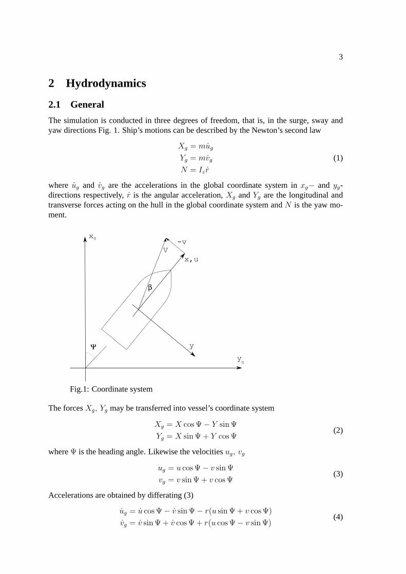
The simulation is conducted in three degrees of freedom, that is, in the surge, sway andyaw directions Fig. 1. Ship’s motions can be described by the Newton’s second law

Xg = mug

Yg = mvg

N = Iz r

(1)

where ug and vg are the accelerations in the global coordinate system inxg− and yg-directions respectively,r is the angular acceleration,Xg andYg are the longitudinal andtransverse forces acting on the hull in the global coordinate system andN is the yaw mo-ment.

Fig.1: Coordinate system

The forcesXg, Yg may be transferred into vessel’s coordinate system

Xg = X cos Ψ− Y sin Ψ

Yg = X sin Ψ + Y cos Ψ(2)

whereΨ is the heading angle. Likewise the velocitiesug, vg

ug = u cos Ψ− v sin Ψ

vg = v sin Ψ + v cos Ψ(3)

Accelerations are obtained by differating (3)

ug = u cos Ψ− v sin Ψ− r(u sin Ψ + v cos Ψ)

vg = v sin Ψ + v cos Ψ + r(u cos Ψ− v sin Ψ)(4)

4

Finally the forcesX, Y andN can be evaluated by substituting (2), (3) and (4) into (1)

X = m(u− vr)

Y = m(v − ur)

N = Iz r

(5)

Depending on the mathematical model, the total forcesX, Y andN are divided to severalcomponents,

X = Xh + Xr + Xpr + Xi

Y = Yh + Yr + Ypr + Yi

N = Nh + Nr + Npr + Ni

(6)

whereXh, Yh andNh are the hull forces,Xr, Yr, Nr are the rudder forces,Xpr, Ypr, Npr

the propulsion forces andXi, Yi, Nh are the ice forces.

Finally, the drift angle can be calculated as follows

β = tan(−v

u

)(7)

2.2 Hull Forces

The forces acting on the hull (6) are assumed to be functions of the ship’s state of motion

Xh = Xh(u, u, v, v, r, r)

Yh = Yh(u, u, v, v, r, r)

Nh = Nh(u, u, v, v, r, r)

(8)

(8) can be approximated using Taylor series (onlyX-component given as an example)

Xh = X0+[Xuu + Xvv + Xrr + Xuu + Xvv + Xrr

]+

1

2!

[Xuuu|u|+ Xvvv|v|+ Xrrr|r|+ ... + 2Xurur + ... + 2Xvrvr

]+

1

3!

[Xuuuu

3 + Xvvvv3|+ Xrrrr

3 + ... + 6Xuvruvr + ... + 6Xuvruvr]

+ ...

(9)

It should be reminded, that the terms in (9) include all physics in open water environment,that is, also the free surface effects. In ice conditions vessel’s own wave system should beexcluded from the hull forces.

2.3 Abkowitz Model

Abkowitz model is based on Taylor series (9) so that the Taylor expansion contains alsothe propulsion forces and the rudder forces. The Taylor series are expanded up to the third

5

degree terms as follows [5]

Xh =X0 + Xu∆u + Xuu∆u2 + Xuuu∆u3 + Xvvv2 + (Xrr + mxg)r

2+

Xδδδ2 + (Xvr + m)vr + Xrδrδ + Xvδvδ

Yh =Y0 + Yvv + Yvvvv3 + Yvδδvδ2 + (Yr −mu)r + Yrvvrv

2+

Yδδ + Yδδδδ3 + Yδvvδv

2

Nh =N0 + Nvv + Nvvvv3 + Nvδδvδ2 + (Nr −mxgu0)r + Nrvvrv

2+

Nδδ + Nδδδδ3 + Nδvvδv

2

(10)

wherexg is the longitudinal location of centre of gravity andXδ, Yδ, ... terms represent therudder forces.∆u is utilized to simulate different velocities, that is

∆u = u− u0 (11)

whereu0 is the desired velocity for the simulation.

3 Ice Forces

3.1 Some Definitions of Concepts and Variables

The ice forces are divided to breaking, crushing and submersion components followingthe ideas presented by Lindqvist [2]. As the original theory is a 2D-theory, the methodis extended to 3D in order to match the demands of manoeuvring simulation models. Thephysics of crushing was also adjusted, since the proposed method allows the crushing of iceto occur anywhere along the waterline. The original method [2] assumed that the crushingtakes primaly place in the bow area.

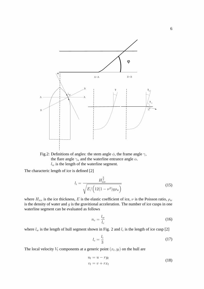
The required parameters to describe the hull shape are presented in Fig. 2. The anglesφ,γ, γn andα are related to each other as follows

cot γn = tan γ cos α (12)

and

tan γn =tan φ

sin α(13)

For the proposed method the trigonometric functions are replaced by the vector notations,expect for the submersion formulas. The hull normal pointing outwards from the hullsurface is normalized as follows √

n2x + n2

y = 1 (14)

6

Fig.2: Definitions of angles: the stem angleφ, the frame angleγ,the flare angleγn and the waterline entrance angleα.lw is the length of the waterline segment.

The characteric length of ice is defined [2]

li =H

32ice√

E/(12(1− ν2)gρw

) (15)

whereHice is the ice thickness,E is the elastic coefficient of ice,ν is the Poisson ratio,ρw

is the density of water andg is the gravitional acceleration. The number of ice cusps in onewaterline segment can be evaluated as follows

nc =lwlc

(16)

wherelw is the length of hull segment shown in Fig. 2 andlc is the length of ice cusp [2]

lc =li3

(17)

The local velocityVl components at a generic point(xl, yl) on the hull are

ul = u− ryl

vl = v + rxl

(18)

7

so that the normalized local velocityVn components can be written as follows

un =ul

|~Vl

|

vn =vl

|~Vl|

(19)

The hull is assumed to have a contact to ice, if the scalar product of the local velocity andthe hull normal is positive

~Vl · ~n > 0 (20)

3.2 Crushing of Ice

In [2] the average vertical force acting on the stem area is estimated as follows

Fchz =1

2σbH

2ice (21)

whereσb is the bending strength of ice. The resistance force due the crushing of ice can bewritten as follows

Rc = Fchz ·tan φ + µ cos φ

cos γn

1− µ sin φcosΘ

(22)

For the proposed method, the vertical force is determined using both the ice thickness andthe length of the crushing zone

Fcz =1

2σbHicelr (23)

The crushing zone is limited by the projection of ice cusp’s length

lr = 0.045nclw

(~n · ~Vn

)(24)

so that the crushing force can be written as follows

~Fcr = Fcz

( 1

|nz|+ µ

)~n (25)

whereµ is the friction coeffient between ice and hull surface and~Fcr = (Xcr~i Ycr

~j)T . Theaffect of friction is still evaluated in 2D, as the the ice cusps are assummed to move alongthe x-axis.

The velocity dependency is evaluated according [2] reminding that at the state of rest thereexists no crushing forces

Xcr(u) = Xcr

( |ul|√gHice

)1.3

Ycr(v) = Ycr

( |vl|√gHice

)0.5(26)

8

For the time being, the crushing force rises from zero gradually as the velocity increases.That is, there is no step in the crushing force at zero speed in order to get vessel movingfrom the state of rest.

Finally, the crushing force components inx- andy-directions and the yaw moment can bedetermined as follows

Xc =∑

waterline

Xcr(u)

Yc =∑

waterline

Ycr(v)

Nc =∑

waterline

[−Xcr(u)yl + Ycr(v)xl

] (27)

3.3 Bending of Ice

The starting point is the icebreaking resistance [2]

Rb =(27

64

)σbB

H32ice√

E/(12(1− ν2)gρw

)(tan γn +

µ cos φ

cos γn sin α

)(1 +

1

cos γn

)(28)

whereB is the beam of a ship.The average force along the hull required to break one ice cusp is

Fn =(27

64

)σblw

(H32ice

lc

)(1 +

√1 + n2

z

)(29)

The bending force components are obtained as follows

~Fbe = ncFn

( 1

|nz|+ µ

)~n (30)

where~Fbe = (Xbe~i Ybe

~j)T . The z-component of the normalnz is limited as follows

γn ≤ 89◦ (31)

The effect of velocity is evaluated by the same manner as with the crushing components

Xbe(u) = Xbe

( |ul|√gHice

)1.3

Ybe(v) = Ybe

( |vl|√gHice

)0.5(32)

9

Once the distribution of the bending force is determined, the global forces can be calculatedby summing the bending componentsXbe, Ybe over the waterline as follows

Xb =∑

waterline

Xbe(u)

Yb =∑

waterline

Ybe(v)

Nb =∑

waterline

[−Xbe(u)yl + Ybe(v)xl

] (33)

3.4 Submersion of Ice

In [2] the submersion component is determined by evaluating the loss of potential energy.The resistance is

Rs = ∂ρgHice

(T (B + T )

B + 2T+ µ(Au + cos φ cos γnAf )

)(34)

where the approximated area of flat bottom is approximated

Au = B(0.7L− T

tan φ− 0.25

B

tan α

)(35)

and the total bow area is calculated as follows

Af = BT

√1

sin2 φ+

1

tan2 α(36)

Unlike the crushing and breaking forces, the submersion force is evaluated directly as aglobal force utilizing (34) as follows

Xs = −Rs cos β

Ys = −Rs sin β

Ns = 0.25 · LwlRs sin β

(37)

The submersion components are also functions of velocity, that is

Xs(u) = Xs

[(25.0

|u|√g lwl

)0.7

+(100.0

( |ur|g

+|vr|g

))0.7]Ys(u) = Ys

(25.0

|v|√g lwl

)0.7

Ns(r) = Ns

(100.0

|r|l wl

√g lwl

)0.7

(38)

4 Numerical Method

The total forces are obtained by adding the ice forces to the hydrodynamic forces (10)

X = Xh + Xice

Y = Yh + Yice

N = Nh + Nice

(39)

10

The state of motion at the new time level can be determined by utilizing the Euler explicitFinite Difference Scheme

un+1 = un + ∆tun

vn+1 = vn + ∆tvn

rn+1 = rn + ∆trn

(40)

wheren denotes the time level and∆t is the time step used in simulation. The systemof equations (10) forY andN - that is , for thev andr-velocities - is connected. Theinstantious acceleration components are solved simultanously

du

dt=

X

m−Xu

dv

dt=

(Izz −Nr)Y + YrN

(m− Yv)(Izz −Nr)−NvYr

dr

dt=

(m− Yv)N + NvY

(m− Yv)(Izz −Nr)−NvYr

(41)

Finally, the location of vessel in the global coordinate system is evaluated as follows

xn+1g = xn + ∆t

(un cos Ψn − vn sin Ψn

)yn+1

g = yn + ∆t(un sin Ψn + vn cos Ψn

)Ψn+1 = Ψn + ∆trn

(42)

5 Calculated Cases

5.1 USCGC Mobile Bay

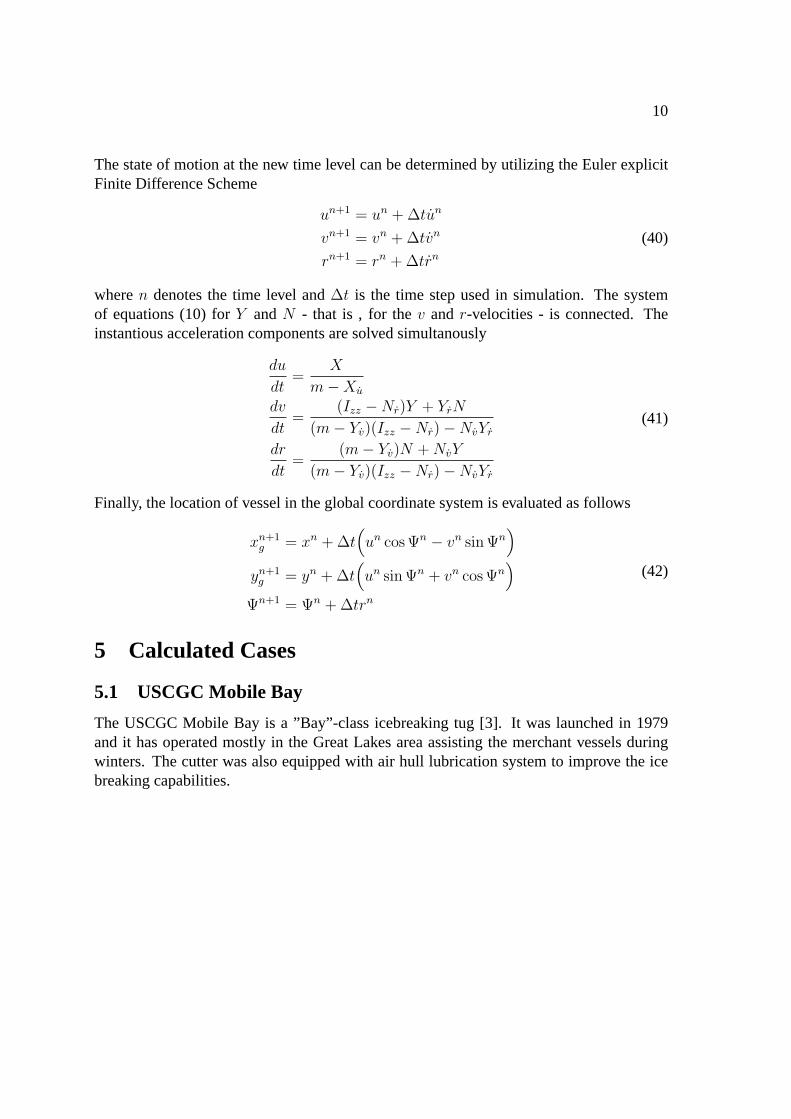
The USCGC Mobile Bay is a ”Bay”-class icebreaking tug [3]. It was launched in 1979and it has operated mostly in the Great Lakes area assisting the merchant vessels duringwinters. The cutter was also equipped with air hull lubrication system to improve the icebreaking capabilities.

11

In 1992 Mobile Bay was transformed from icebreaking tug to a multi-mission tug. Themain particulars are given in Table 1 [1], and the waterplane is shown in Fig 3.

Lwl 39.6 mBwl 10.4 mT 3.7 m4 660 t

Table 1: Main particulars ofUSCGC Mobile Bay.

-30

-20

-10

0

10

20

30

-30 -20 -10 0 10 20 30

x [m

]

y [m]

Fig.3: Mobile Bay’s waterplane.

5.2 MT Uikku

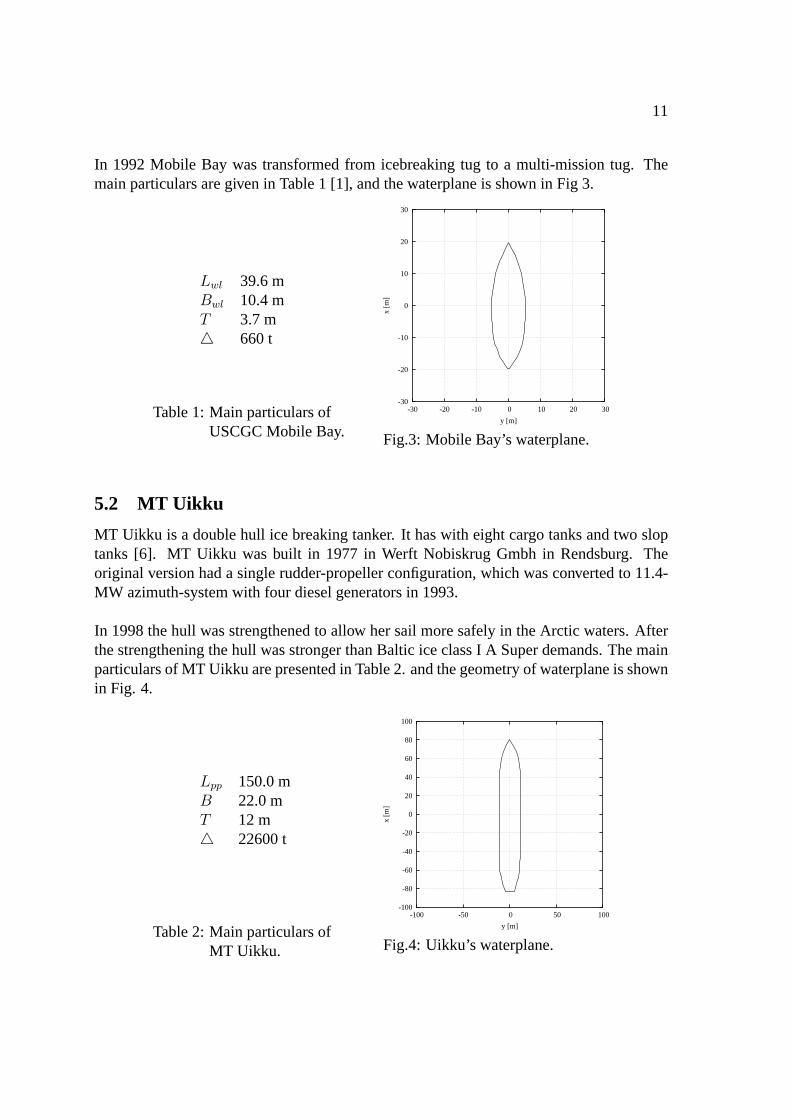
MT Uikku is a double hull ice breaking tanker. It has with eight cargo tanks and two sloptanks [6]. MT Uikku was built in 1977 in Werft Nobiskrug Gmbh in Rendsburg. Theoriginal version had a single rudder-propeller configuration, which was converted to 11.4-MW azimuth-system with four diesel generators in 1993.

In 1998 the hull was strengthened to allow her sail more safely in the Arctic waters. Afterthe strengthening the hull was stronger than Baltic ice class I A Super demands. The mainparticulars of MT Uikku are presented in Table 2. and the geometry of waterplane is shownin Fig. 4.

Lpp 150.0 mB 22.0 mT 12 m4 22600 t

Table 2: Main particulars ofMT Uikku.

-100

-80

-60

-40

-20

0

20

40

60

80

100

-100 -50 0 50 100

x [m

]

y [m]

Fig.4: Uikku’s waterplane.

12

5.2.1 Ice Model Tests of MT Uikku

The model tests were conducted in TKK Ship Laboratory’s ice model basin. The modelscale was 1:31.56, and the model was equipped with a propulsion unit featuring a singlepropeller. During tests the model was manoeuvred by the turnable rudder. The ice sheetwas ensured to have uniform quality during the test procedure.

The summary of tests is presented in Table 3. The first two tests were executed in iceconditions and the last two tests in open water conditions. Eight channels were recorded,that is, the position of the model, the revolutions of propeller, the thrust and the momentof the propeller and finally the rudder angle the and heading angle. The test procedure wasarranged so that the propeller revolutions were kept as constant in all tests.

Test 1 Turning circle

Hice 0.6mσB 550kPAn 120RPMRudder angle 30◦

Test 2 Turning circle

Hice 0.6 mσB 550kPAn 120RPMRudder angle 20◦

Test 3 Turning circle

Hice - mσB - kPAn 120RPMRudder angle 30◦

Test 4 Turning circle

Hice - mσB - kPAn 120RPMRudder angle 20◦

Table 3: Summary of MT Uikku’s tests. The data isgiven in full scale.

6 Results

6.1 Ice Resistance

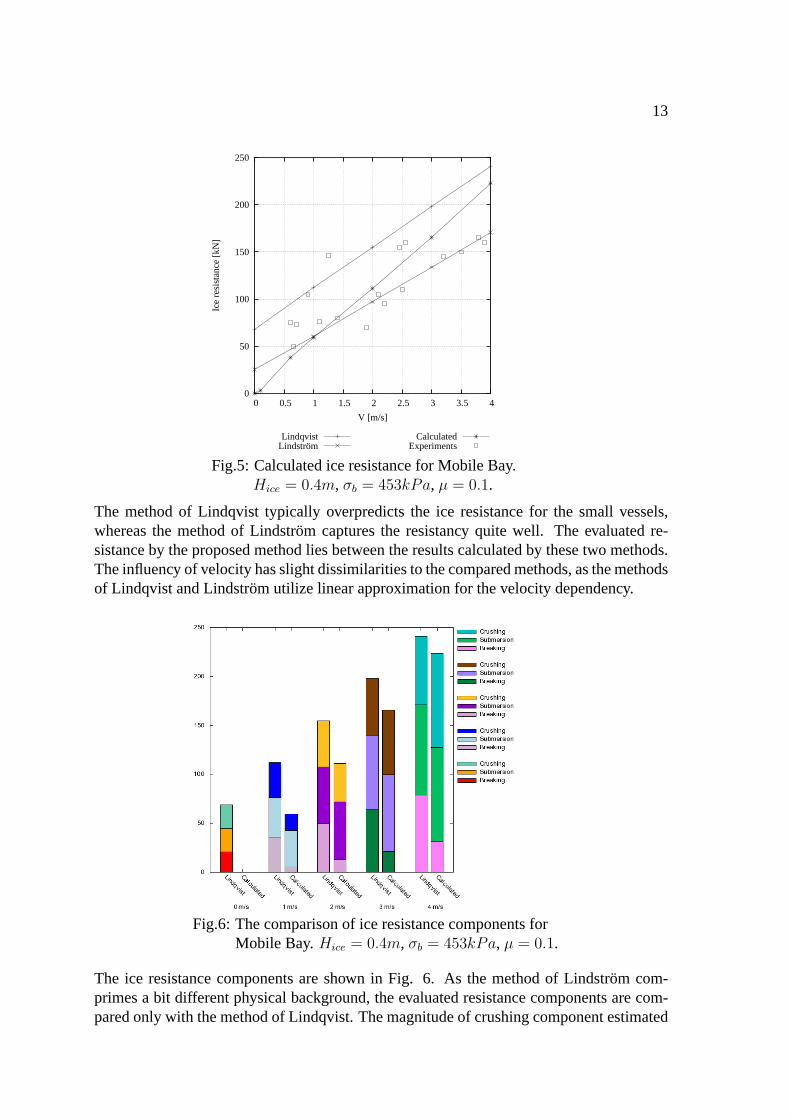
The ice resistance is evaluated using USCGC Mobile Bay as the validation case. The cal-culated ice resistance is compared with the results published in [4]. The total ice resistancecomputed by the proposed method and by two semiempirical methods [2], [1] as well asthe experimental results are presented in Fig. 5.

13

0

50

100

150

200

250

0 0.5 1 1.5 2 2.5 3 3.5 4

Ice

resi

stan

ce [k

N]

V [m/s]

LindqvistLindström

CalculatedExperiments

Fig.5: Calculated ice resistance for Mobile Bay.Hice = 0.4m, σb = 453kPa, µ = 0.1.

The method of Lindqvist typically overpredicts the ice resistance for the small vessels,whereas the method of Lindstrom captures the resistancy quite well. The evaluated re-sistance by the proposed method lies between the results calculated by these two methods.The influency of velocity has slight dissimilarities to the compared methods, as the methodsof Lindqvist and Lindstrom utilize linear approximation for the velocity dependency.

Fig.6: The comparison of ice resistance components forMobile Bay.Hice = 0.4m, σb = 453kPa, µ = 0.1.

The ice resistance components are shown in Fig. 6. As the method of Lindstrom com-primes a bit different physical background, the evaluated resistance components are com-pared only with the method of Lindqvist. The magnitude of crushing component estimated

14

by the method of Lindqvist seems to be relatively larger in small velocities, whereas themagnitude of submersion and breaking components remain almost same for all velocities.The formulas adapted for the submersion force are almost identical in both models, sincethe submersion force is evaluated also as a global force in the proposed method.

It should be still reminded, that the proposed method predicts the ice resistance to be zeroat the state of rest. This could be also changed so, that there would be certain limit forthe vessel’s trust to get the vessel moving. Since the current model was validated usingAbkowitz-simulation model, this kind of limitation was not implemented.

6.2 Turning Circle

The turning circle test with USCGC Mobile Bay were simulated using three different rud-der angles. The ice thickness varied between0.3...0.6 m.

-80

-60

-40

-20

0

20

40

60

80

100

120

-180 -160 -140 -120 -100 -80 -60 -40 -20 0 20

x [m

]

y [m]

Steady turning radius

Fig.7: Turning circle, steady turning radius.

In Fig. 7. is shown a typical turning circle simulation and the steady turning circle radius.The steady turning radiuses are compared in Fig. 8. both with the measured data andsimulated results [1].

15

40

60

80

100

120

140

160

180

200

220

240

0.3 0.35 0.4 0.45 0.5 0.55 0.6

R [m

]

Ice thickness [m]

Lindström 30Lindström 20Lindström 10

Experiment 10Experiment 20

Experiment 30Calculated 30Calculated 20Calculated 10

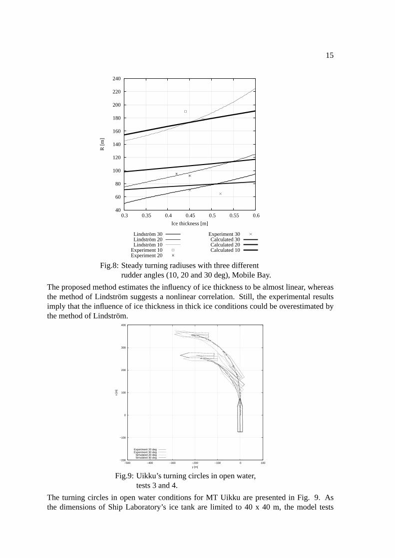
Fig.8: Steady turning radiuses with three differentrudder angles (10, 20 and 30 deg), Mobile Bay.

The proposed method estimates the influency of ice thickness to be almost linear, whereasthe method of Lindstrom suggests a nonlinear correlation. Still, the experimental resultsimply that the influence of ice thickness in thick ice conditions could be overestimated bythe method of Lindstrom.

−200

−100

0

100

200

300

400

−500 −400 −300 −200 −100 0 100

x [m

]

y [m]

Experiment 20 degExperiment 30 deg

Simulated 20 degSimulated 30 deg

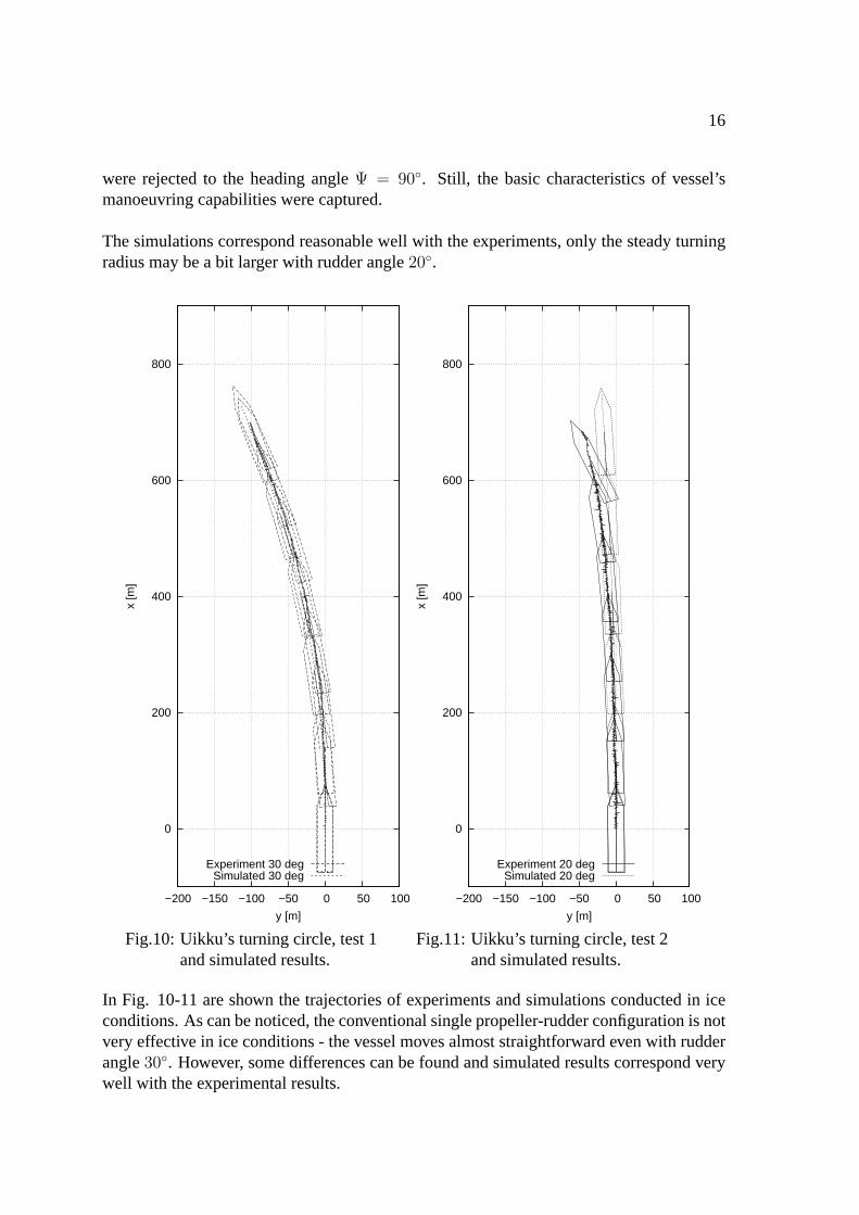
Fig.9: Uikku’s turning circles in open water,tests 3 and 4.

The turning circles in open water conditions for MT Uikku are presented in Fig. 9. Asthe dimensions of Ship Laboratory’s ice tank are limited to 40 x 40 m, the model tests

16

were rejected to the heading angleΨ = 90◦. Still, the basic characteristics of vessel’smanoeuvring capabilities were captured.

The simulations correspond reasonable well with the experiments, only the steady turningradius may be a bit larger with rudder angle20◦.

0

200

400

600

800

−200 −150 −100 −50 0 50 100

x [m

]

y [m]

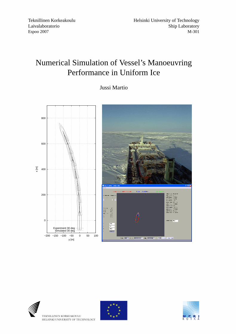
Experiment 30 degSimulated 30 deg

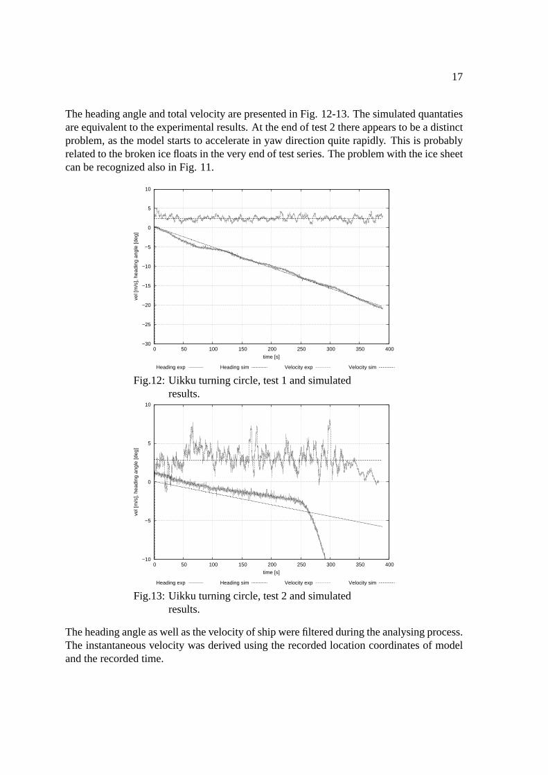
Fig.10: Uikku’s turning circle, test 1and simulated results.

0

200

400

600

800

−200 −150 −100 −50 0 50 100

x [m

]

y [m]

Experiment 20 degSimulated 20 deg

Fig.11: Uikku’s turning circle, test 2and simulated results.

In Fig. 10-11 are shown the trajectories of experiments and simulations conducted in iceconditions. As can be noticed, the conventional single propeller-rudder configuration is notvery effective in ice conditions - the vessel moves almost straightforward even with rudderangle30◦. However, some differences can be found and simulated results correspond verywell with the experimental results.

17

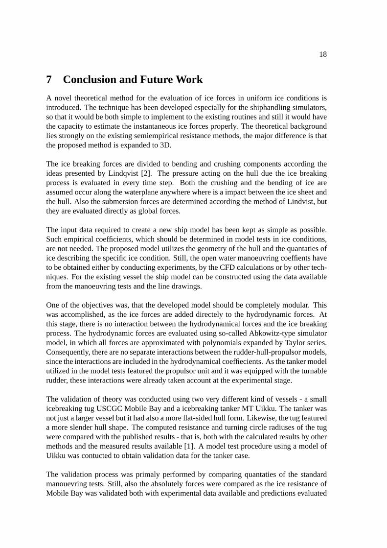
The heading angle and total velocity are presented in Fig. 12-13. The simulated quantatiesare equivalent to the experimental results. At the end of test 2 there appears to be a distinctproblem, as the model starts to accelerate in yaw direction quite rapidly. This is probablyrelated to the broken ice floats in the very end of test series. The problem with the ice sheetcan be recognized also in Fig. 11.

−30

−25

−20

−15

−10

−5

0

5

10

0 50 100 150 200 250 300 350 400

vel [

m/s

], he

adin

g an

gle

[deg

]

time [s]

Heading exp Heading sim Velocity exp Velocity sim

Fig.12: Uikku turning circle, test 1 and simulatedresults.

−10

−5

0

5

10

0 50 100 150 200 250 300 350 400

vel [

m/s

], he

adin

g an

gle

[deg

]

time [s]

Heading exp Heading sim Velocity exp Velocity sim

Fig.13: Uikku turning circle, test 2 and simulatedresults.

The heading angle as well as the velocity of ship were filtered during the analysing process.The instantaneous velocity was derived using the recorded location coordinates of modeland the recorded time.

18

7 Conclusion and Future Work

A novel theoretical method for the evaluation of ice forces in uniform ice conditions isintroduced. The technique has been developed especially for the shiphandling simulators,so that it would be both simple to implement to the existing routines and still it would havethe capacity to estimate the instantaneous ice forces properly. The theoretical backgroundlies strongly on the existing semiempirical resistance methods, the major difference is thatthe proposed method is expanded to 3D.

The ice breaking forces are divided to bending and crushing components according theideas presented by Lindqvist [2]. The pressure acting on the hull due the ice breakingprocess is evaluated in every time step. Both the crushing and the bending of ice areassumed occur along the waterplane anywhere where is a impact between the ice sheet andthe hull. Also the submersion forces are determined according the method of Lindvist, butthey are evaluated directly as global forces.

The input data required to create a new ship model has been kept as simple as possible.Such empirical coefficients, which should be determined in model tests in ice conditions,are not needed. The proposed model utilizes the geometry of the hull and the quantaties ofice describing the specific ice condition. Still, the open water manoeuvring coeffients haveto be obtained either by conducting experiments, by the CFD calculations or by other tech-niques. For the existing vessel the ship model can be constructed using the data availablefrom the manoeuvring tests and the line drawings.

One of the objectives was, that the developed model should be completely modular. Thiswas accomplished, as the ice forces are added directely to the hydrodynamic forces. Atthis stage, there is no interaction between the hydrodynamical forces and the ice breakingprocess. The hydrodynamic forces are evaluated using so-called Abkowitz-type simulatormodel, in which all forces are approximated with polynomials expanded by Taylor series.Consequently, there are no separate interactions between the rudder-hull-propulsor models,since the interactions are included in the hydrodynamical coeffiecients. As the tanker modelutilized in the model tests featured the propulsor unit and it was equipped with the turnablerudder, these interactions were already taken account at the experimental stage.

The validation of theory was conducted using two very different kind of vessels - a smallicebreaking tug USCGC Mobile Bay and a icebreaking tanker MT Uikku. The tanker wasnot just a larger vessel but it had also a more flat-sided hull form. Likewise, the tug featureda more slender hull shape. The computed resistance and turning circle radiuses of the tugwere compared with the published results - that is, both with the calculated results by othermethods and the measured results available [1]. A model test procedure using a model ofUikku was contucted to obtain validation data for the tanker case.

The validation process was primaly performed by comparing quantaties of the standardmanouevring tests. Still, also the absolutely forces were compared as the ice resistance ofMobile Bay was validated both with experimental data available and predictions evaluated

19

by two calculation methods. The influency of ice thickness was validated by comparing thesimulated static turning radiuses using different rudder angles and various ice thicknesses.Also the effect of velocity was tested, as the ice resistance was evaluated with severalvelocities. The sway force and yaw moment were not analyzed in this study.

The model tests of MT Uikku were conducted both in open water and ice conditions.The open water experiments were utilized for the determination of the hydrodynamic co-effiecients, and the ice tests were applied for the validation of the ice model. The manoeu-vring capabilities in ice conditions were very limited, since the vessel featured a conven-tional single rudder-propeller configuration and a flat-sided hull form.

The simulated results of both vessels correspond reasonable well with the validation data.The calculated resistance of proposed method is between the two methods compared. Also,the magnitudes of ice force components are similar to components determined by themethod with same physical background. The velocity dependencity is formulated so, thatthe ice force grows gradually as the the ship starts to move from the state of rest. Still, theproposed method was able to capture the main characteristics of very different type of turn-ing circles - Mobile Bay had reasonable desent manoeuvring behaviour in ice conditionswhereas the MT Uikku with conventional single propeller-rudder configuration producedvery large turning circle radiuses.

In the future the sway force and yaw moment could be also validated and compared toexperimental results. This requires that the global forces in forced static and dynamicmotions are measured. Furthermore, as the proposed model evaluates the crushing andbending forces acting on the hull, it would be interesting to compare directly the forcesacting on the waterplane segments. This could be accomplished also by the full scale mea-surements. The yaw and sway forces due the submersion of ice cusps were not validated.The validation process for these components is far more complicated than the comparisonof the crushing and bending forces.

There are several possibilities to improve the evaluation of ice breaking process. Oneoption is to determine the geometry of the ice cusps accurately in time domain. This canbe unfortunately quite time consuming, since the theoretical foundation of such methodwould probably lie on the Partial Differential Equations. Furthermore, the proposed methoddoes not contain the history of ice crushing process, ie. the model does not contain anyenvironmental information. The interaction between ice and water could be modelled moreproperly. The simplest way to accomplish this could be utilizing semiempirical formulas,which coefficients should be determined in model tests.

As the model is limited to uniform ice conditions, the next step could be to expand themodel to include ice-packs and ice channels. Unfortunately these would require informa-tion from the environment around the vessel, so a simple mathematical simulation modelaimed primaly for hydrodynamic studies can be a inconvinient platform to start the de-velopment of such packages. Also the existence of mixed ice-water substance around thevessel could be taken into account.

20

It should be also mentioned, that the proposed method can be utilized in the developmentof visualizing tools for the integrated bridge simulators. The theory determines the averagesize of broken ice cusps and the number of cusps along the waterline segments. Since theactual breaking is not simulated in the time domain, the actual geometry of the ice floes isnot available.

21

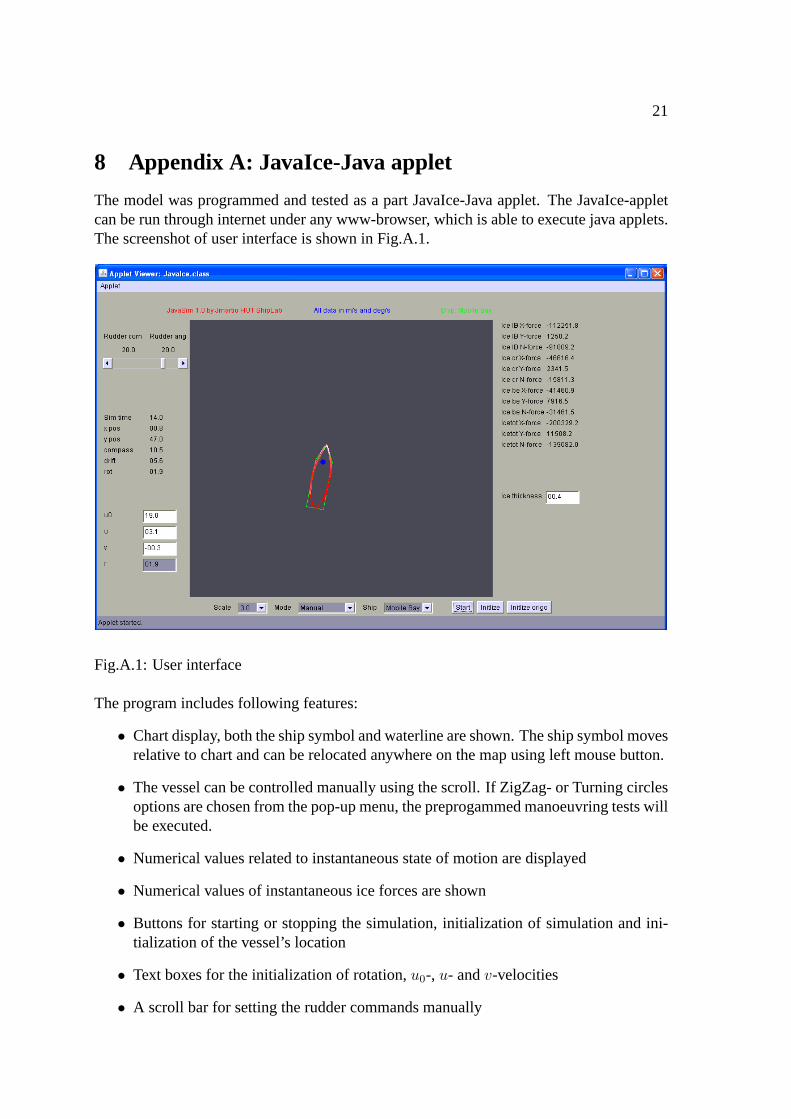
8 Appendix A: JavaIce-Java applet

The model was programmed and tested as a part JavaIce-Java applet. The JavaIce-appletcan be run through internet under any www-browser, which is able to execute java applets.The screenshot of user interface is shown in Fig.A.1.

Fig.A.1: User interface

The program includes following features:

• Chart display, both the ship symbol and waterline are shown. The ship symbol movesrelative to chart and can be relocated anywhere on the map using left mouse button.

• The vessel can be controlled manually using the scroll. If ZigZag- or Turning circlesoptions are chosen from the pop-up menu, the preprogammed manoeuvring tests willbe executed.

• Numerical values related to instantaneous state of motion are displayed

• Numerical values of instantaneous ice forces are shown

• Buttons for starting or stopping the simulation, initialization of simulation and ini-tialization of the vessel’s location

• Text boxes for the initialization of rotation,u0-, u- andv-velocities

• A scroll bar for setting the rudder commands manually

22

• A pop-up menu for setting the scale of chart and ship symbol

• A pop-up menu to choice the vessel, ie. MT Uikku or USCGC Mobile Bay

• A text box to set the ice thickness

• The pressure caused by ice breaking - crushing and bending components - are visual-ized in the chart display. The vessel’s waterline changes color according the pressure- the white color denotes high pressure, red means no contact with the ice

23

References

[1] Lindstrom C-A. Prediktering av fartygs manoverformaga i jamn is genom simuleringav planrorelserna.Master Thesis, HUT Ship Laboratory, 1989.

[2] Lindqvist G. A straightforward method for calculation of ice resistance of ships.POAC, pages 722–735, 1989.

[3] URL: http://www.uscg.mil/d9/grumil/unit/sturgeonbay/cgcmobilebay/cgcmobilebay1.html.

[4] Kamarainen J. Evaluation of ship ice resistance calculation methods.Licenciate Thesis,HUT Ship Laboratory, 1993.

[5] HUT Ship Laboratory.Lecture notes: Marine Hydrodynamics, advanced course.

[6] Hanninen S. Ship based observations onboard mt uikku during the winter 2003.IRIS-project, EVK3-CT-2002-00083, 2003.

SHIP LABORATORYPublished M-series reports:

M-287 T. Leiviska; LAIVAN PROPULSIOKERTOIMET JAISSA JA AVOVEDESSA. OSA 1: KE-VAAN 2002 MALLIKOESARJAN MITTAUSRAPORTTI. OSA 2: MITTAUSTULOSTENANALYYSI JA PROPULSIOKERTOIMIEN TARKASTELU. Otaniemi 2004.

M-288 J. Romanoff, A. Klanac; DESIGN FORMULATIONS FOR FILLED STRUCTURALSANDWICH PANES. Otaniemi 2005.

M-289 J. Matusiak; LAIVAN KULKUVASTUS. Otaniemi 2005.

M-290 J. Kajaste-Rudnitski, P. Varsta, J. Matusiak; SOME FE ESTIMATES OF SHIPCOLLISION EVENT. Otaniemi 2005.

M-291 J. Romanoff, H. Remes, G. Socha, M. Jutila; STIFFNESS AND STRENGTH TESTINGOF LASER STAKE WELDS IN STEEL SANDWICH PANELS. Otaniemi 2006.

M-292 P. Ruponen; MODEL TESTS FOR THE PROGRESSIVE FLOODING OF A BOX-SHAPEDBARGE. Otaniemi 2006.

M-293 T. Mikkola; UNSTRUCTURED PRESSURE-CORRECTION METHOD BASED ONTRIANGLE MESHES. Otaniemi 2006.

M-294 T. Arola, R. Jalonen, P. Kujala; MERILIIKENTEEN PAIKKATIEDON TILASTOINTI JAHYODYNTAMINEN SUOMENLAHDEN MERITURVALLISUUDESSA. Otaniemi 2007.

M-295 J. Kajaste-Rudnitski, P. Varsta, K. Tabri; COLLISION RESISTANCE OF CERTAIN SIDESTRUCTURES OF RO-RO PASSENGER SHIP. Otaniemi 2007.

M-296 A. Munir; MARINE DIESEL ENGINE EXHAUST GAS SYSTEM, FOULING ANDCORROSION PROBLEMS. Otaniemi 2007.

M-297 J. Ranta, K. Tabri; STUDY ON THE PROPERTIES OF POLYURETHANE FOAM FORMODEL-SCALE SHIP COLLISION EXPERIMENTS. Otaniemi 2007.

M-298 M. Jutila, J. Romanoff; LASERHITSATUN TERAKSISEN KERROSLEVYPALKINKOLMIPISTETAIVUTUSKOKEET. Otaniemi 2007.

M-299 M. Hanninen, P. Kujala; MERILIIKENTEEN YHTEENTORMAYS- JA KARILLEAJO-RISKIEN MALLINNUS. KIRJALLISUUSKATSAUS. Otaniemi 2007.

M-300 T. Arola; PAIKKATIETOTYOKALUT SUOMENLAHDEN MERENKULUN RISKIARVIOINNISSA.Otaniemi 2007.

ISBN 978-951-22-9067-3ISSN 1456-3045