numerical investigation of the performance and flow
TRANSCRIPT
Numerical Investigation of the
Performance and Flow Behaviour of
Centrifugal Compressors
A Thesis Submitted to the University of Manchester for the
Degree of Master of Philosophy in the Faculty of Engineering
and Physical Sciences
2014
Yu Ang Wu
School of Mechanical, Aerospace and Civil Engineering

i | P a g e
Contents
Abstract ............................................................................................... iv
Acknowledgements ......................................................................... vi
Declaration ....................................................................................... vii
Restriction ....................................................................................... viii
Nomenclature .................................................................................... ix
List of Figures .................................................................................. xii
List of Tables .................................................................................. xvii
Chapter 1 Introduction .................................................................... 1
1.1. Background............................................................................................................................................ 1
1.2. Motivation and Objectives ............................................................................................................... 4
1.3. Outline of Thesis .................................................................................................................................. 5
Chapter 2 Literature Review ......................................................... 7
2.1. Introduction .......................................................................................................................................... 7
2.2. Centrifugal Compressor Fundamentals ..................................................................................... 7
2.2.1. Compressor Performance ...................................................................................................... 7
2.2.2. Impeller ...................................................................................................................................... 13
2.2.3. Diffuser ....................................................................................................................................... 14
2.2.4. Compressor Flow Phenomenon ....................................................................................... 15
2.2.5. Losses in Compressor ........................................................................................................... 20
2.3. Existing Works on Centrifugal Compressor .......................................................................... 26
2.4. Existing Works on Riblets............................................................................................................. 34
2.4.1. Turbulent Skin Friction Drag Reduction ....................................................................... 34
2.4.2. Delay of Laminar-Turbulent Transition ........................................................................ 41
2.5. Discussion ........................................................................................................................................... 42
Chapter 3 Turbulence Modelling .............................................. 44
3.1. Introduction ....................................................................................................................................... 44
ii | P a g e
3.2. Reynolds Averaged Navier-Stokes Equations ...................................................................... 47
3.3. Eddy Viscosity Model ..................................................................................................................... 48
3.3.1. Zero Equation Model ............................................................................................................. 49
3.3.2. One Equation Model .............................................................................................................. 49
3.3.3. Two Equation Model ............................................................................................................. 50
3.4. Reynolds Stress Model ................................................................................................................... 53
3.5. Summary .............................................................................................................................................. 55
Chapter 4 Methods of Investigation ......................................... 56
4.1. Introduction ....................................................................................................................................... 56
4.2. Assumptions ....................................................................................................................................... 56
4.3. Turbomachinery Modelling Techniques ................................................................................ 57
4.4. Grid Generation................................................................................................................................. 58
4.4.1. Block-Structured Mesh......................................................................................................... 58
4.4.2. Polyhedral Unstructured Mesh ......................................................................................... 60
4.5. Numerical Conditions ..................................................................................................................... 60
4.5.1. Turbulence Parameters Estimation ................................................................................ 61
4.5.2. Boundary Conditions ............................................................................................................ 62
4.5.3. Wall treatments ....................................................................................................................... 63
4.5.4. Convergence Criteria ............................................................................................................ 63
4.6. Loss Localization Method ............................................................................................................. 64
4.7. Summary .............................................................................................................................................. 64
Chapter 5 Validation of Star CCM+ Solver .............................. 66
5.1. Introduction ....................................................................................................................................... 66
5.2. CD-adapco Star CCM+ Solver....................................................................................................... 66
5.3. Validation with Performance Evaluation ............................................................................... 68
5.3.1. Dyson V2 Centrifugal Compressor .................................................................................. 68
5.3.2. Numerical Conditions ........................................................................................................... 70
5.3.3. Results ......................................................................................................................................... 72
5.4. Validation with Flow Field Analysis ......................................................................................... 75
5.4.1. ERCOFTAC Centrifugal Compressor ............................................................................... 75
5.4.2. Numerical Conditions ........................................................................................................... 77
5.4.3. Results ......................................................................................................................................... 78
5.5. Summary .............................................................................................................................................. 83
Chapter 6 Flow Field Analysis .................................................... 85

iii | P a g e
6.1. Introduction ....................................................................................................................................... 85
6.2. Results .................................................................................................................................................. 85
6.3. Summary .............................................................................................................................................. 99
Chapter 7 Effects of Unsteadiness ........................................... 101
7.1. Introduction ..................................................................................................................................... 101
7.2. Results ................................................................................................................................................ 101
7.3. Summary ............................................................................................................................................ 110
Chapter 8 Application of Riblets ............................................. 111
8.1. Introduction ..................................................................................................................................... 111
8.2. Further Discussions on Riblets ................................................................................................. 111
8.3. Riblets on Dyson V2 Impeller.................................................................................................... 118
8.4. Effects of Unsteadiness ................................................................................................................ 123
8.5. Summary ............................................................................................................................................ 125
Chapter 9 Conclusions and Future Work ............................. 126
9.1. Conclusions ....................................................................................................................................... 126
9.2. Future Work ..................................................................................................................................... 127
Reference ........................................................................................ 129
Appendix A Comparisons Between Turbulence Models . 137
Appendix B Grid Independence Study .................................. 139

iv | P a g e
Abstract
Centrifugal compressor is of great importance in industries. High efficiency, high
stage pressure ratio, wide operation range, easy to manufacture and easy to
maintain make it prevalent in aerospace, automobile and power generation
industries. The possibility in improving its efficiency has been pursued all the way
along its path of development. Nowadays, energy-saving has been a key
competitiveness for any power-consuming product. Dyson V2 centrifugal
compressor is powered by a high speed electric motor, and provides suction power
to the upstream cyclone separator to separate the dust particles from the air. It is
highly desirable that the efficiency can be improved such that less electricity would
be consumed. As the first step to improve its efficiency, it is essential to gain some
knowledge on the flow phenomena involved, in essence, efficiency is the direct
reflection of the quality of the flow field. The flow is viscous, highly unsteady,
swirling and transitional inside Dyson V2 centrifugal compressor, strong
interaction exists between different flow features, the compound effects of strong
curvature, centrifugal force and Coriolis force make it very difficult to obtain an
acceptable prediction. Theoretical approach is usually too ideal to take into account
different flow features, experimental approach is too costly and generally time-
consuming. With the rapid development of CFD techniques and the availability of
high performance computers, computational approach is becoming one of the most
popular tools during design and development phases.
In this work, computational approach has been employed to investigate the
performance and the flow behaviour inside the Dyson V2 centrifugal compressor.
Validation studies are first conducted to examine the capability of Star CCM+ solver,
good agreements are obtained with the experimental data. After that, the flow field
inside the Dyson V2 centrifugal compressor is analysed using steady simulation,
which is relatively easy to conduct and feasible during the design phase. Different
flow phenomena, including tip leakage flow, separation bubble, “jet-wake
v | P a g e
structure" and corner separation are observed. Vortex roll-up process is identified,
it is initialized near the impeller blade leading edge due to tip leakage flow, and
grows in the axial part of the impeller, finally, it decays in the radial part of the
impeller due to centrifugal force. A loss localization method is employed to identify
the sources of significant loss generation, it is found that tip leakage flow is the
most significant source of loss, it is initialized near the blade leading edge through
vortex roll-up, and very difficult to control. The endwall loss and blade surface loss
associated with boundary layer are significant near the impeller outlet and blade
suction-side due to the high flow speed, corner separation induced loss in diffuser
is also significant. Later, the effects of unsteadiness are investigated through
unsteady simulation, it is shown that unsteadiness can help weaken or suppress
flow separation and lead to reduced blockage and local loss generation. The
impeller-diffuser interaction tends to slow down the high speed flow near the
impeller blade suction-side and migrate the high speed flow from suction-side to
pressure-side.
In literature, riblets have been extensively tested, although the physical
mechanisms are not fully understood, it is definitely sure that riblets with proper
size can help reduce the turbulent skin friction drag. In this work, riblets have been
proposed to reduce the impeller hub endwall loss. However, riblets are of very
small size, fully resolved simulation is extremely time-consuming and costly. Curve
fitting is applied to correlate the available experimental data on riblets, an
expression has been obtained to relate the wall shear stress reduction to non-
dimensional spacing and yaw-angle. The riblets are designed and optimized based
on the wall shear stress computed from steady simulation, the design value for wall
shear stress reduction is around 4%. At the end, the riblets performance is assessed
with unsteady simulation, it is confirmed that the riblets design based on steady
simulation could perform very well, even under the effects of unsteadiness, a wall
shear stress reduction around 4% could be achieved.

vi | P a g e
Acknowledgements
First and foremost, I would like to thank my supervisor Dr. Shan Zhong for her
patient supervision and fruitful discussion, and my co-supervisor Prof Lin Li for his
useful comments on my work.
I am also indebt to Dr. Alistair Revell, who has been my tutor and friend since my
undergraduate course, without the discussion with him, the work would not have
been possible.
I also would like to thank my colleagues, Yuan Ye Zhou, Tian Long See, Omonigho
Otanocha, Fernando Valenzuela Calva and Jesus Garcia Gonzalez for their help and
friendship during the year at Manchester.
This work is supported by Dyson Ltd., discussions with Dr. Mark Johnson, Dr.
Andrew Bower, Mr. Owen Nicholson and Dr. Adair Williams during the regular
meetings are greatly appreciated.
At last, I would like to express my sincere thanks to my parents, without their
continuous love and support, I would not have been here.

vii | P a g e
Declaration
No portion of the work referred to in this thesis has been submitted in support of
an application for another degree or qualification of this or any other university or
other institute of learning.

viii | P a g e
Restriction
This project is funded by Dyson Ltd., the Dyson V2 centrifugal compressor
geometry and experimental results are supplied by Dyson, these materials are
subjected to the confidential restrictions, and should not be distributed to public
without the permission of Dyson Ltd.

ix | P a g e
Nomenclature
A Area C� Blade surface length C� Dissipation coefficient C� Pressure coefficient/Specific heat at constant pressure C�� Base pressure coefficient
D Diameter D� Hydraulic diameter
div Divergence
grad Gradient
h Height
I Turbulence intensity
i Internal energy
k Thermal conduction coefficient/Turbulent kinetic energy
L Length
l Turbulence length scale l� Mixing length
M Mach number m Mass flow rate
N Rotational speed (rpm)
P Power/Perimeter
p Pressure
Q Volume flow rate
Re Reynolds number Reθ Momentum thickness Reynolds number
r Radius S � Total rate of entropy generation per unit area
s Entropy/Spacing
T Temperature
t Thickness/Time
U Rotational speed (m/s) uτ Friction velocity
V Absolute velocity V� Blade surface velocity
W Relative velocity
β Clauser pressure gradient parameter
β� Backsweep angle � Specific heat constant
δ Boundary layer thickness
ε Turbulent dissipation rate � Efficiency/Kolmogorov length scale
θ Momentum boundary thickness

x | P a g e
κ Karman constant
μ Dynamic viscosity
ν Kinematic viscosity
ν� Eddy diffusivity
ξ Entropy loss coefficient
ω Rotational speed (rad/s)/Specific dissipation coefficient
ρ Density
τ Shear stress
τη Kolmogorov time scale
Abbreviations
AW Air Watt
CFD Computational Fluid Dynamics
DNS Direct Numerical Simulation
ERCOFTAC European Research Community On Flow Turbulence and
Combustion
FVM Finite Volume Method
L2F Laser-2-Focus
LA Laser Anemometry
LES Large Eddy Simulation
LSCC Low Speed Centrifugal Compressor
MACE Mechanical, Aerospace and Civil Engineering
PS Pressure-Side
PIV Particle Image Velocimetry
PJSW Pressure-side Jet and Suction-side Wake
PWSJ Pressure-side Wake and Suction-side Jet
RANS Reynolds Averaged Navier-Stokes equations
RSM Reynolds Stress Model
SA Spalart Allmaras
SGS Sub-Grid Scale
SS Suction-Side
SST Shear Stress Transport
TS Tollmien-Schlichting
Superscripts and Subscripts
c Cross-stream/Compressor
m Main stream
r Radial component
s Static condition
t Stagnation condition
w Wake
θ Tangential component
0 Stagnation condition
1 Impeller inlet
2 Impeller outlet/Diffuser inlet

xi | P a g e
3 Diffuser outlet
+ Non-dimensional quantity
* Relative stagnation condition
xii | P a g e
List of Figures
Chapter 1
Figure 1- 1: Heron's steam rotor (Fransson, Hillon and Klein, 2000). 2
Figure 1- 2: Rolls-Royce Trent 1000 onboard a Boeing 787 dreamliner
during flight.1
2
Figure 1- 3: Dyson V2 digital motor.2 3
Figure 1- 4: Different types of compressors (Dixon, 2010). 3
Figure 1- 5: Schematic of Dyson Vacuum Cleaner System. 4
Chapter 2
Figure 2- 1: Performance characteristic of a compressor (Dixon, 2010). 9
Figure 2- 2: General compressor flow streamline with velocity triangle. 11
Figure 2- 3: Different types of impeller blading. 14
Figure 2- 4: Pressure-side and suction-side legs of horseshoe vortex (Chen,
Papailiou and Huang, 1999).
16
Figure 2- 5: Laminar separation bubble formation process. 17
Figure 2- 6: Tip leakage flow for an unshrouded impeller (Denton, 1993). 18
Figure 2- 7: Two types of jet-wake structures at impeller outlet. 19
Figure 2- 8: Secondary flow in cross section normal to streamwise direction. 20
Figure 2- 9: Mixing of injected flow with main stream (Denton, 1993). 23
Figure 2- 10: Different types of riblets. 35
Figure 2- 11: Drag reduction performance of various rib geometries
(Bechert et al., 1997a).
36
Figure 2- 12: Comparison of drag reduction ratio reproduced from El-Samni,
Chun and Yoon (2007).
38
xiii | P a g e
Figure 2- 13: Schematic of streamwise vortex interaction with riblets
surface via viscous effects (Bacher and Smith, 1985).
41
Chapter 3
Figure 3- 1: Laminar and turbulent flow patterns (Reynolds, 1901). 45
Chapter 4
Figure 4- 1: Blunt trailing edge impeller blocking strategy. 59
Figure 4- 2: Curved leading and trailing edge diffuser blocking strategy. 59
Chapter 5
Figure 5- 1: NASA X-34 re-entry simulation with Star CCM+ (Courtesy of TLG
Aerospace).
67
Figure 5- 2: Polyhedral mesh on a UAV (Courtesy of CD-adapco). 67
Figure 5- 3: Dyson V2 impeller configuration (including impeller and
diffuser).
68
Figure 5- 4: Dyson V2 steady simulation configuration. 71
Figure 5- 5: Dyson V2 impeller block-structured mesh. 71
Figure 5- 6: Dyson V2 vaned diffuser block-structured mesh. 72
Figure 5- 7: Streamwise cross section mesh for Dyson V2 impeller. 72
Figure 5- 8: Dyson V2 centrifugal compressor stage performance airwatt
curve.
73
Figure 5- 9: Dyson V2 centrifugal compressor stage performance efficiency
curves.
74
Figure 5- 10: Dyson V2 centrifugal compressor performance pressure ratio
curves.
75
Figure 5- 11: ERCOFTAC centrifugal pump 2D blade impeller. 76
Figure 5- 12: ERCOFTAC centrifugal pump 2D blade diffuser. 76
Figure 5- 13: Non-dimensioanl radial velocity at time instant T=0.126. 79

xiv | P a g e
Figure 5- 14: Non-dimensional radial velocity at time instant T=0.226. 79
Figure 5- 15: Non-dimensional radial velocity at time isntant T=0.326. 80
Figure 5- 16: Non-dimensional radial velocity at time instant T=0.426. 80
Figure 5- 17: Non-dimensional tangential velocity at time instant 0.126 81
Figure 5- 18: Non-dimensional tangential velocity at time instant 0.226. 82
Figure 5- 19: Non-dimensional tangential velocity at time instant 0.326. 82
Figure 5- 20: Non-dimensional tangential velocity at time instant 0.426. 83
Chapter 6
Figure 6- 1: Dyson V2 centrifugal compressor sub-regions. 86
Figure 6- 2: Circumferential-averaged Relative Mach number contour for
impeller meridional plane.
87
Figure 6- 3: Relative Mach number contour for impeller S plane at 90%
blade span.
88
Figure 6- 4: Relative Mach number contour for impeller S planes at a) 10%,
b) 50% blade span.
89
Figure 6- 5: Relative velocity contour on four streamwise stations with
streamlines.
89
Figure 6- 6: Relative Mach number contour for impeller outlet. 89
Figure 6- 7: Relative velocity contour on stations 1 to 4. 90
Figure 6- 8: Skin friction lines on impeller casing. 91
Figure 6- 9: Circumferential-averaged static pressure (Pa) contour in the
impeller meridional plane.
92
Figure 6- 10: Velocity vector for impeller S plane at 60% blade span. 92
Figure 6- 11: Total entropy generation rate per unit volume �W/�m�K�� on
stations 1 to 4.
93
Figure 6- 12: Wall shear stress (Pa) contour with skin friction lines on
impeller blade and hub (a) suction-side, (b) pressure-side.
94
Figure 6- 13: Mach number contour for radial and axial diffusers S planes at
(a) 10% span, (b) 50% span, (c) 90% span.
95
xv | P a g e
Figure 6- 14: Incidence angle (deg) contour for radial diffuser at (a) 10%,
(b) 50%, (c) 90% blade span.
96
Figure 6- 15: Total entropy generation rate per unit volume �W/�m�K�� on
stations 5 to 9.
97
Figure 6- 16: Circumferential-averaged static pressure (Pa) contour for
radial and axial diffusers at meridional plane.
98
Figure 6- 17: Cross-section-averaged static pressure in streamwise
direction.
98
Chapter 7
Figure 7- 1: Performance comparison between steady and unsteady
simulations.
102
Figure 7- 2: Relative Mach number contour for steady and unsteady
simulations on stations 1 to 4 (top to bottom) in impeller region.
103
Figure 7- 3: Mach number contour for steady and unsteady simulations on
stations 5 to 9 (top to bottom) in diffuser region.
104
Figure 7- 4: Local entropy generation rate per unit volume �W/�m�K��
contour from steady and unsteady simulations on station 4 (left column)
and station 6 (right column) for different time instant.
106
Figure 7- 5: Relative Mach number contour at impeller outlet from unsteady
simulation. (The leading edge of radial diffuser blade is marked as black bar,
the impeller blade trailing edge is marked as black trapezoid).
107
Figure 7- 7: Wall shear stress (Pa) contour with skin friction lines on
impeller hub, predicted from steady and unsteady simulations (top view).
109
Chapter 8
Figure 8- 1: General structure of a wall shear stress reduction curve with
riblets (Bechert et al., 1997a).
112
Figure 8- 2: Sawtooth riblets dimensions. 113
Figure 8- 3: Wall shear stress reduction for sawtooth riblets obtained from
Walsh and Lindemann (1984) with curve fitting.
114
Figure 8- 4: Yaw-angle effect on riblets performance with data cited from
Walsh and Lindemann (1984).
115

xvi | P a g e
Figure 8- 5: Top view of the scallop shell. (Anderson, Macgillivray and
Demont, 1997)
116
Figure 8- 6: Magnified view of scallop shell. (Anderson, Macgillivray and
Demont, 1997)
116
Figure 8- 7: Wall shear stress distribution on test plate. (Bechert et al., 1997) 118
Figure 8- 8: Top view of Dyson V2 impeller with the application of riblets. 120
Figure 8- 9: Circumferential stations on hub to apply riblets. 120
Figure 8- 10: Wall shear stress distribution on 7 stations. 121
Figure 8- 11: Optimum riblets spacing on different stations. 121
Figure 8- 12: Maximum wall shear stress reduction on different stations. 122
Figure 8- 13: Wall shear stress distribution on station 7. 123
Figure 8- 14: Yaw-angle distribution on station 7. 124
Figure 8- 15: Wall shear stress reduction on different stations under the
effects of unsteadiness.
124
Appendix A
Figure A- 1: AirWatt Plot for different turbulence models. 137
Figure A- 2: Total-to static isentropic efficiency for different turbulence
models.
138
Figure A- 3: Static pressure ratio for different turbulence models. 138
Appendix B
Figure B- 1: Static pressure plot at impeller hub mid-pitch for different grid
resolutions.
140
Figure B- 2: Wall shear stress plot at impeller hub mid-pitch for different
grid resolutions.
140
Figure B- 3: Static pressure plot at impeller blade mid-span for different grid
resolutions.
141
Figure B- 4: Wall shear stress plot at impeller blade mid-span for different
grid resolutions.
141

xvii | P a g e
List of Tables
Chapter 2
Table 2- 1: Comparison of optimum geometry of different riblets (Dean,
2011).
36
Table 2- 2: Different riblets surface configurations (Wang et al., 2008). 37
Table 2- 3: Drag reduction efficiency of different riblets configurations
(Wang et al., 2008).
37
Chapter 5
Table 5- 1: Dyson V2 centrifugal compressor geometry parameters. 69
Table 5- 2: Dyson V2 centrifugal compressor performance evaluation cases. 70
Table 5- 3: ERCOFTAC centrifugal pump geometry and operation
parameters (Ubaldi et al., 1996).
77
Chapter 8
Table 8- 1: A summary of the curve fitting for sawtooth riblets. 116
Appendix B
Table B- 1: Summary of block-structured mesh. 139

1 | P a g e
Chapter 1 Introduction
Introduction
1.1. Background
Turbomachine is a rotary device that exchanges energy with the working fluid
through blade rotation. According to either extracting or adding energy,
turbomachine can be broadly classified into two categories, turbine and
compressor (air) or pump(water) respectively.
Turbomachine has gone through a slow and long process of development. The
steam engine designed by the Heron of Alexandria is probably one of the first
turbomachines, as shown in Figure 1- 1, the steam goes out from the ball as two
opposite oriented jets, thus propelling force is produced from the conservation of
momentum. Other forms of early turbomachinery application are windmills and
waterwheels, which extract energy from wind and moving water respectively, then
the retrieved energy can be applied to grind grain and pump water. Nowadays,
some of them are still in operation and mainly for tourism purpose.
Human beings technologies develop rapidly, and most of them are power
demanding, nowadays, more energy is required than ever before. Some of the most
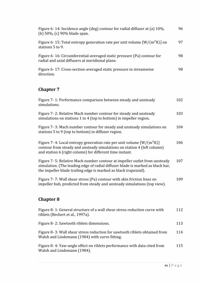
common turbomachines are gas turbine engine onboard aircraft (Figure 1- 2),
hydraulic turbine in the dam, Dyson V2 centrifugal compressor in a Dyson handheld
vacuum cleaner (Figure 1- 3), turbocharger inside a car, and even the heart pumps
implanted in human body. Extensive research has been conducted on
turbomachinery efficiency improvement, nowadays, the efficiency of large
2 | P a g e
turbomachine can reach as high as 97% (hydraulic pump), while that of small
turbomachine is still relatively low, about 70%. The problem encountered by the
small turbomachine is that the flow is subject to strong curvature, centrifugal force
and Coriolis force, and the small cross-sectional area constrains the flow, as a result,
the flow behaviour is very complicated, strong interactions exist between different
flow features, what's worse, the small size makes the application of flow control
devices prohibited. Flow features such as viscous, unsteady, three-dimensional,
transitional and strong interaction make it difficult to obtain a reliable prediction,
some of the physical mechanisms are still poor understood.
Figure 1- 1: Heron's steam rotor (Fransson, Hillon and Klein, 2000).
Figure 1- 2: Rolls-Royce Trent 1000 onboard a Boeing 787 dreamliner during
flight.1
1: Retrieved from http://www.rolls-royce.com/civil/products/largeaircraft/trent_1000/

3 | P a g e
Figure 1- 3: Dyson V2 digital motor.2
Being used to efficiently transfer energy to the working fluid in the form of raised
pressure level, compressor has been widely employed in aerospace, power
generation and process industries. Various types of compressor exist, each suitable
for a specific application. Axial flow compressor is capable of working with large
amount of working fluid at one time with relatively small frontal area, which is very
critical in aerospace application (drag consideration), although the stage pressure
ratio is low, multi-stage arrangement could achieve overall pressure ratio as high
as 40:1. In contrary, centrifugal flow compressor can only handle a limited amount
of working fluid, while it can achieve stage pressure ratio as high as 8:1, majorly
due to the contribution from the centrifugal force. A compromise between flow
capacity and pressure ratio brings us to the mixed flow compressor. Figure 1- 4
presents a sketch of different types of compressors.
Figure 1- 4: Different types of compressors (Dixon, 2010).
Turbomachine has been an integral part of our life, wide application and power-
consuming make it stringent to improve its efficiency. Tremendous amount of
2: Retrieved from http://www.dyson.co.uk/vacuumcleaners/ddm.aspx
4 | P a g e
efforts have been expended to improve the turbomachinery efficiency, and it will
continue in the foreseeable future. Centrifugal compressor, as a kind of
turbomachine, has evolved from low efficiency, poor designed to high efficiency, 3D
well designed machine, however, small centrifugal compressor is still of relatively
low efficiency due to its inherent complex flow interaction. So it is essential to
understand the flow behaviour involved. Recently, Computational Fluid Dynamics
(CFD) gains its popularity in both research and engineering design due to its
relatively low cost, short return cycle and the capability in revealing more flow
features compared to theoretical and experimental approaches. The development
of CFD techniques enables the designer to have a more comprehensive view on the
flow behaviour involved and the general performance.
1.2. Motivation and Objectives
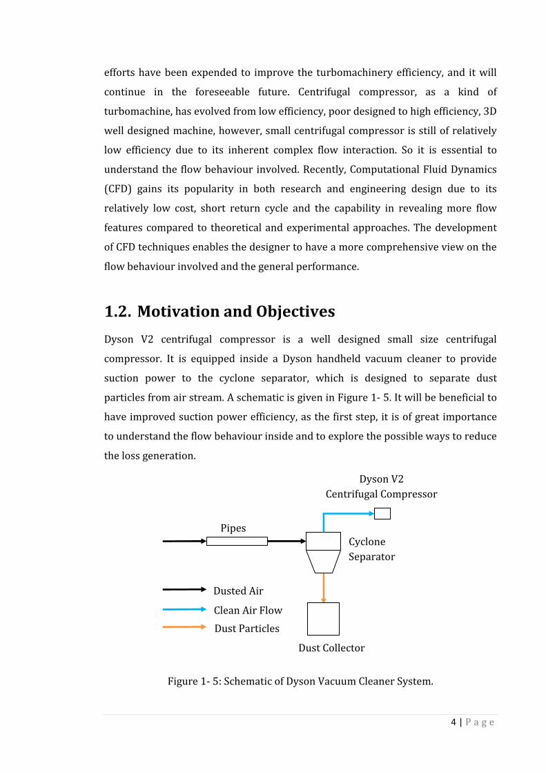
Dyson V2 centrifugal compressor is a well designed small size centrifugal
compressor. It is equipped inside a Dyson handheld vacuum cleaner to provide
suction power to the cyclone separator, which is designed to separate dust
particles from air stream. A schematic is given in Figure 1- 5. It will be beneficial to
have improved suction power efficiency, as the first step, it is of great importance
to understand the flow behaviour inside and to explore the possible ways to reduce
the loss generation.
Figure 1- 5: Schematic of Dyson Vacuum Cleaner System.
Cyclone
Separator
Pipes
Dyson V2
Centrifugal Compressor
Dust Collector
Dusted Air
Clean Air Flow
Dust Particles
5 | P a g e
The objectives of this work is to analyse the performance and flow behaviour of
Dyson V2 centrifugal compressor, find regions of high loss and investigate the
effect of unsteadiness, at the end, it is thus possible to provide methods for
improving the Dyson V2 centrifugal compressor performance.
1.3. Outline of Thesis
The whole thesis is subdivided into several chapters.
Chapter 2 intends to introduce the basic compressor theory, including the
performance characteristics, commonly observed flow phenomena and sources of
loss generation, after that, the existing experimental and numerical works on
centrifugal compressor are reviewed. At the end, riblets, as a kind of passive flow
control devices, have been surveyed and reviewed in details.
Chapter 3 introduces the turbulence modelling materials, at the beginning, the
Navier-Stokes equations and RANS are described, then different RANS models are
discussed and compared as well as the corresponding formulations.
Chapter 4 describes the method of investigation for this work, first of all, the
assumptions made in this work are given as the basis for the following studies.
Then a brief introduction to the turbomachinery modelling techniques is provided,
followed by the discussion on grid generation and numerical conditions. At the end,
the loss localization method is introduced, with the explicit expressions, it is
possible to identify regions of high local loss generation.
The solver validation is given in Chapter 5, experimental data are available for
Dyson V2 centrifugal compressor and ERCOFTAC centrifugal compressor with
regard to performance and flow field respectively. Single passage steady simulation
is conducted for performance validation with Dyson V2 centrifugal compressor,
while full annulus unsteady simulation is performed for flow field validation with
ERCOFTAC centrifugal compressor.
Detailed flow field analysis on Dyson V2 centrifugal compressor is conducted in
Chapter 6 using steady simulation. The general flow behaviour with regard to the
performance is presented, distinct flow features are identified. Loss localization

6 | P a g e
method has been applied to spot regions of high local loss generation, the
important sources of loss generation are identified. Wall shear stress distribution
and hub skin friction lines are obtained and will be used for riblets design in
chapter 8.
In chapter 7, full annulus unsteady simulation is performed, the effect of
unsteadiness on Dyson V2 centrifugal compressor performance and flow field is
discussed. Particular attention has been paid to the variation in wall shear stress on
hub, this information will be used in chapter 8 to assess the riblets performance
under the effects of unsteadiness.
Chapter 8 presents some further discussions on the application of riblets, including
operation regimes, optimization and yaw-angle effect. An explicit expression has
been obtained by conducting curve fitting on experimental data to relate the wall
shear stress reduction to the non-dimensional spacing. Later, riblets are proposed
to be applied to the Dyson V2 impeller hub to reduce the hub endwall loss, steady
simulation results are used to design the riblets, at the end, the riblets performance
is assessed using unsteady simulation.
Finally, conclusions are drawn in chapter 9, discussions on future work are also
made to shed light on possible further developments in the future.
7 | P a g e
Chapter 2 Literature Review
Literature Review
2.1. Introduction
In this chapter, a brief introduction to the compressor theory will be given at first,
including the general performance characteristics and centrifugal compressor
components, the typical flow phenomena occurred in centrifugal compressor and
loss generation, with emphasis on centrifugal compressor with unshrouded
impeller and vaned diffuser. After that, existing works on centrifugal compressor
are discussed to shed light on the current status of research on centrifugal
compressor, including both experimental and numerical approaches. At the end,
riblets surface is introduced as a passive flow control method, existing works on
riblets performance in case of flat plates, pipes and compressors are also reviewed.
2.2. Centrifugal Compressor Fundamentals
2.2.1. Compressor Performance
Compressor is an equipment to increase the energy of the working fluid, its
performance has to be assessed according to several general performance
parameters, such as isentropic efficiency, pressure ratio, operation range, pressure
coefficient and etc, details are given as follows.

8 | P a g e
Isentropic Efficiency
Isentropic efficiency is a parameter relating the real process to the ideal isentropic
process, which is free from heat transfer and loss, it characterizes how much
entropy has been generated due to the loss(irreversibility) for the real process.
Depending on whether the exhaust has been utilized or not, the isentropic
efficiency can be classified into two subcategories, total-to-total isentropic
efficiency(Eqn 2-1) and total-to-static isentropic efficiency(Eqn 2-2) respectively.
The former is applied if the exhaust is used to produce further work, such as that
for aircraft gas turbine engines, conversely, in the case of gas turbine in power
generation station, the exhaust discharges into the atmosphere(in some cases, the
exhaust is used for heating in houses) directly, the latter should be applied.
η�,� = "#$%&,'%&,()*+(*"#,&,',&,( Eqn 2- 1
η�,- = "#$%.,'%&,()*+(*"#,&,',&,( Eqn 2- 2
Pressure Ratio
Compressor works to increase the static and total pressure of the working fluid,
therefore, static and total pressure ratios are important performance parameters,
however, higher static or total pressure ratio does not necessarily mean higher
work output, which depends on the specific performance parameter for certain
application. In the case of a reasonably well designed impeller, both static and total
pressure of the working fluid at the outlet should be increased compared to those
at inlet, the static pressure would also increase for diffuser due to the diffusion
process, however, the total pressure would reduce for diffuser due to losses and
lack of work input.

9 | P a g e
Operation Range
In most cases, compressor would not work at a fixed operation condition, instead, it
will operate at different mass flow rates and speeds according to the loading
condition and application, these make the compressor a rather dynamic machine,
generally, it should possess high efficiency at a variety of operation conditions.
More importantly, it has to be able to withstand sudden unstable inflow conditions
and restore the original state as soon as possible.
Figure 2- 1: Performance characteristic of a compressor (Dixon, 2010).
The whole operation could be summarised in a performance map(as shown in
Figure 2- 1), with which some of the operation conditions could be described easily,
the lines of constant efficiency are in the form of closed curves, which could be
called the efficiency islands. Referring to Figure 2- 1, the compressor should work
at the maximum efficiency point at the design operation condition, ideally, the
operation path should pass through the peak efficiency point, as denoted by the red

10 | P a g e
line. At the design operation condition, the inlet flow should be well matched to the
blade leading edge and go smoothly along the blade, as shown in part (a) Figure 2-
2, the streamlines are shown in the rotating reference frame. Referring to part (b)
Figure 2- 2, if the mass flow rate at the inlet is increased, while the rotation speed is
kept constant, the blade incidence angle would reduce considerably, and the inlet
and outlet velocity will be increased, thus lead to reduced static pressure,
continuous increase in mass flow rate at inlet would bring the impeller to choke
condition, for which the flow will reach the speed of sound at the throat, as a result,
further increase in mass flow rate inside the impeller is not achievable. In contrary,
a decrease in inlet mass flow rate at constant speed would reduce the inlet velocity,
near leading edge separation may happen and cause stall (part (c), Figure 2- 2), the
loss increases dramatically, more seriously, the compressor surge would occur and
bring significant impact on the performance, stability and the blade life.
Pressure Coefficient
The pressure recovery coefficient is generally applied to assess the diffuser
performance, it describes to what extent the diffuser inlet dynamic pressure could
be converted into static pressure. Therefore, it is formally defined as the ratio of
static pressure rise to diffuser inlet dynamic pressure, as given in Eqn 2-3.
C�/ = �0#�'�&,'#�' Eqn 2- 3
Similarly, the pressure loss coefficient can be defined as:
C�1 = �&,'#�&,0�&,'#�' Eqn 2- 4
Suction Power
The general performance parameters has been introduced, there is one more
application specific performance parameter has to be introduced. The Dyson V2
centrifugal compressor is equipped inside a Dyson handheld vacuum cleaner, for

Figure 2- 2: General compressor flow streamline
Free Stream
Free Stream
Free Stream
Blade Rotation
Blade Rotation
Blade Rotation
W
W
: General compressor flow streamline with velocity triangle
Blade Rotation
Blade Rotation
Blade Rotation
W1
W2
U
V2
V2
U2
V1
U1
U1
V1
U1
V1
W1
W1
W2
W2
V2, θ
V2, r
V2, θ
V2, θ
V2, r
V2
V2, r
11 | P a g e
with velocity triangle.
U2
U2
12 | P a g e
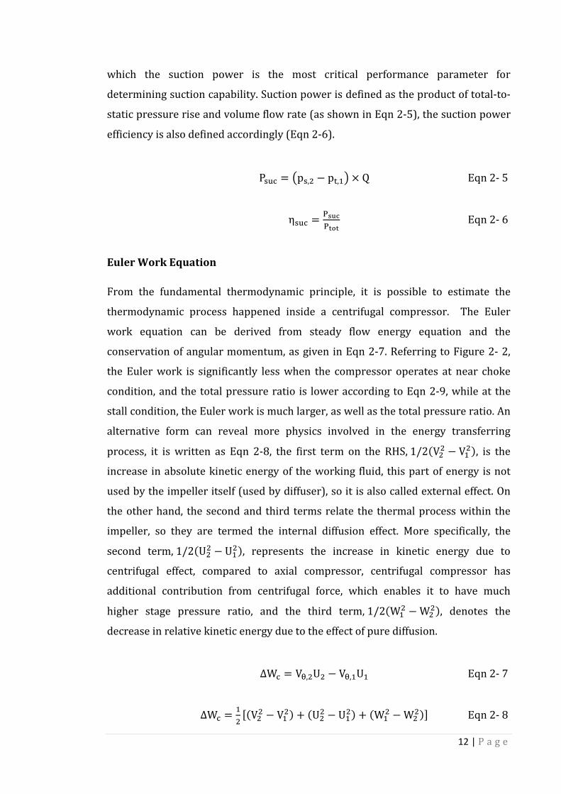
which the suction power is the most critical performance parameter for
determining suction capability. Suction power is defined as the product of total-to-
static pressure rise and volume flow rate (as shown in Eqn 2-5), the suction power
efficiency is also defined accordingly (Eqn 2-6).
P-34 = 5p-,� − p�,"8 × Q Eqn 2- 5
η-34 = ;.<=;&>& Eqn 2- 6
Euler Work Equation
From the fundamental thermodynamic principle, it is possible to estimate the
thermodynamic process happened inside a centrifugal compressor. The Euler
work equation can be derived from steady flow energy equation and the
conservation of angular momentum, as given in Eqn 2-7. Referring to Figure 2- 2,
the Euler work is significantly less when the compressor operates at near choke
condition, and the total pressure ratio is lower according to Eqn 2-9, while at the
stall condition, the Euler work is much larger, as well as the total pressure ratio. An
alternative form can reveal more physics involved in the energy transferring
process, it is written as Eqn 2-8, the first term on the RHS, 1/2�V�� − V"��, is the
increase in absolute kinetic energy of the working fluid, this part of energy is not
used by the impeller itself (used by diffuser), so it is also called external effect. On
the other hand, the second and third terms relate the thermal process within the
impeller, so they are termed the internal diffusion effect. More specifically, the
second term, 1/2�U�� − U"��, represents the increase in kinetic energy due to
centrifugal effect, compared to axial compressor, centrifugal compressor has
additional contribution from centrifugal force, which enables it to have much
higher stage pressure ratio, and the third term, 1/2�W"� − W���, denotes the
decrease in relative kinetic energy due to the effect of pure diffusion.
∆W4 = VC,�U� − VC,"U" Eqn 2- 7
∆W4 = "� ��V�� − V"�� + �U�� − U"�� + �W"� − W���� Eqn 2- 8

13 | P a g e
If there is no heat transfer and irreversibility (isentropic process), the isentropic
total pressure rise could be related to stagnation temperature change. For a
centrifugal compressor impeller with no-swirl inlet flow, the isentropic total-to-
total pressure ratio can be expressed as Eqn 2-9.
�&,'�&,( = $E&,'E&,() **+( = $1 + FG,'H'I%E&,( ) **+(
Eqn 2- 9
Similarly, with the assumption of isentropic process, the total pressure should be
constant throughout the diffuser. So the stage isentropic total pressure ratio is
exactly the same as that of impeller, as given by Eqn 2-9.
2.2.2. Impeller
The impeller is the rotating component inside a centrifugal compressor, sometimes,
it is also called the compressor wheel. Generally, it consists of a number of blades
with complex profile and curvature, and mounted to the hub. The working fluid is
accelerated to extremely high speed in the impeller, and flung outward with
centrifugal force and Coriolis force produced due to rotation. The impeller design is
critical, it determines whether or not the energy could be efficiently transported to
the working fluid. Impeller can be further divided into two seamlessly merged
sections, inducer and exducer respectively. Inducer is the axial section of the
impeller, for which it largely determine the maximum flow capability. Exducer, on
the other hand, is the radial section of the impeller, it limits the ability to accelerate
the air at a given shaft speed.
Impeller could be categorized according to the types of blading, namely
forwardswept, radial and backswept blade impeller, they are illustrated in Figure
2- 3 with outlet velocity triangles. The backswept impeller produces less Euler
work at given shaft speed, but it has wider operation range and better stability, and
it is usually required to operate at high speed. In contrast, the forwardswept
impeller produces much higher Euler work, however, its operation range is limited
due to the high outlet air speed and small flow angle, it is usually applied where
high pressure ratio is required.

14 | P a g e
Figure 2- 3: Different types of impeller blading.
The impeller blade can be also categorized into shrouded and unshrouded types,
shrouded impeller tends to have higher stress on the blade, thus requires stronger
blade structure, which would undoubtedly increase the weight and limit the shaft
speed to low level. Severe back flow can be observed in the clearance between the
shroud and casing due to the pressure gradient between outlet and inlet. While
unshrouded impeller is more common in recent designs, 3D blade can be relatively
easier to incorporate, thus could improve the efficiency considerably. However,
unshrouded impeller is prone to tip leakage flow, the interaction is much more
complex, thus impact the efficiency. A trade-off study has to be conducted by the
designer to determine the appropriate design for the specific application.
2.2.3. Diffuser
The air flow is of very high speed at the outlet of impeller, generally, almost half of
the shaft power has been expended to raise the speed of the air. So it is of practical
importance to use this part of energy, to serve this purpose, diffuser can be
arranged downstream of the impeller to recover the otherwise wasted energy. The
recovery is in fact a diffusion process, for which the flow has to be slowed done
appropriately, otherwise, severe separation may present and cause deterioration in
performance. The diffusion process can be completed with either vaneless diffuser
or vaned diffuser, the former diffuses the flow by increasing the radius solely, while
the latter employs the double effect of increasing radius and flow turning by vane
curvature. Vaneless diffuser is subject to high skin friction loss and generally of low
efficiency, while the operation range is very wide. Vaned diffuser, as a means to
Forwardswept
U2 U2 U2
V2, θ
V2, θ V2, θ
Radial Backswept
W2
W2 W2 V2, r
V2, r V2, r V2 V2 V2
15 | P a g e
improve the efficiency, is very sensitive to flow condition, the operation range is
rather limited due to possible stall inception at the diffuser blade. On the other
hand, the presence of vaned diffuser will cause impeller-diffuser interaction, which
tends to distort the flow field significantly, the optimum spacing between the
impeller blade and diffuser blade is a critical design parameter, which need to be
determined carefully, otherwise severe loss can occur, and the compressor
performance will be severely impacted.
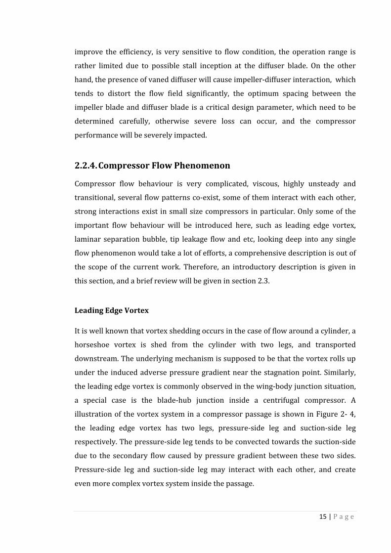
2.2.4. Compressor Flow Phenomenon
Compressor flow behaviour is very complicated, viscous, highly unsteady and
transitional, several flow patterns co-exist, some of them interact with each other,
strong interactions exist in small size compressors in particular. Only some of the
important flow behaviour will be introduced here, such as leading edge vortex,
laminar separation bubble, tip leakage flow and etc, looking deep into any single
flow phenomenon would take a lot of efforts, a comprehensive description is out of
the scope of the current work. Therefore, an introductory description is given in
this section, and a brief review will be given in section 2.3.
Leading Edge Vortex
It is well known that vortex shedding occurs in the case of flow around a cylinder, a
horseshoe vortex is shed from the cylinder with two legs, and transported
downstream. The underlying mechanism is supposed to be that the vortex rolls up
under the induced adverse pressure gradient near the stagnation point. Similarly,
the leading edge vortex is commonly observed in the wing-body junction situation,
a special case is the blade-hub junction inside a centrifugal compressor. A
illustration of the vortex system in a compressor passage is shown in Figure 2- 4,
the leading edge vortex has two legs, pressure-side leg and suction-side leg
respectively. The pressure-side leg tends to be convected towards the suction-side
due to the secondary flow caused by pressure gradient between these two sides.
Pressure-side leg and suction-side leg may interact with each other, and create
even more complex vortex system inside the passage.

16 | P a g e
Figure 2- 4: Pressure-side and suction-side legs of horseshoe vortex (Chen,
Papailiou and Huang, 1999).
Laminar Separation Bubble
In case of low Reynolds number flow, the flow may be laminar at the beginning,
laminar-turbulent transition will occur at some point before the flow becoming
fully turbulent. Transition is a very difficult and broad research topic, although a
vast amount of efforts have been expended on it, the physical mechanism is still not
fully understood at this moment, three different types of transition exist in
literature, natural transition, bypass transition and separation induced transition
respectively. Natural transition seldom happens inside a compressor, instead,
bypass transition is common due to the high turbulence level at the inlet, and
laminar separation bubble would appear in the case of low Reynolds number flow.
Laminar separation bubble is usually caused by the strong adverse pressure
gradient, which could happen due to large local curvature near the blade leading
edge. The initial laminar boundary layer cannot sustain the adverse pressure
gradient, hence separates from the wall. The separated laminar flow is very
sensitive to disturbances, and goes through transition to turbulent flow, if the
transition point is close enough to the wall, the relatively high momentum

17 | P a g e
turbulent flow may reattach to the wall and forms a laminar separation bubble,
otherwise the turbulent flow may not be able to reattach the wall, and thus causes
complete separation of the flow. Figure 2- 5 illustrates the formation of laminar
separation bubble, as indicated by the circulation zone.
Figure 2- 5: Laminar separation bubble formation process.
Tip Leakage Flow
Tip leakage flow exists in both unshrouded and shrouded impeller due to the
existence of unavoidable tip clearance between the blade tip/shroud and the casing.
For the unshrouded impeller, the tip leakage flow is induced by the pressure
difference between the suction-side and pressure-side of the blade, the flow leaks
from the pressure-side to the suction-side under the pressure gradient, while in the
case of shrouded impeller, tip leakage flow occurs due to the pressure difference
between the blade trailing edge and leading edge, and exists inside the clearance
between the shroud and casing. In centrifugal compressor, centrifugal force and
Coriolis force also contribute to the tip leakage flow, however, the resultant effect is
very complicated and varies for different impeller blading (forwardswept, radial or
backswept). The leakage flow rate can be estimated with the pressure difference
and contraction ratio, which is defined to take into account the contraction of the
flow area due to blockage inside the clearance.
Tip leakage flow is always described as a source of disadvantage to the compressor
performance, it can affect the compressor in different ways, first of all, the tip
leakage flow produces significant loss regions near the blade tip, secondly, blockage
can be created in the passage core region due to the separation and vortex roll-up.
turbulent flow
laminar flow
18 | P a g e
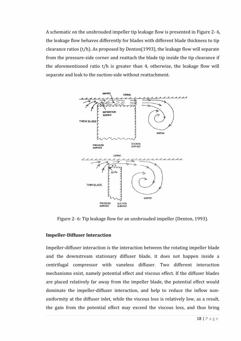
A schematic on the unshrouded impeller tip leakage flow is presented in Figure 2- 6,
the leakage flow behaves differently for blades with different blade thickness to tip
clearance ratios (t/h). As proposed by Denton(1993), the leakage flow will separate
from the pressure-side corner and reattach the blade tip inside the tip clearance if
the aforementioned ratio t/h is greater than 4, otherwise, the leakage flow will
separate and leak to the suction-side without reattachment.
Figure 2- 6: Tip leakage flow for an unshrouded impeller (Denton, 1993).
Impeller-Diffuser Interaction
Impeller-diffuser interaction is the interaction between the rotating impeller blade
and the downstream stationary diffuser blade, it does not happen inside a
centrifugal compressor with vaneless diffuser. Two different interaction
mechanisms exist, namely potential effect and viscous effect. If the diffuser blades
are placed relatively far away from the impeller blade, the potential effect would
dominate the impeller-diffuser interaction, and help to reduce the inflow non-
uniformity at the diffuser inlet, while the viscous loss is relatively low, as a result,
the gain from the potential effect may exceed the viscous loss, and thus bring

positive effect on the
between the diffuser blade and the impelle
loss would increase
effect, thus deteriorate
effects on diffuser, impeller
the upstream impeller in the form
the stall inception. A careful investigation into the
to be done by the designer to achieve better performance and higher operat
stability for the compressor.
Jet-Wake Structure
Jet-wake structure is commonly observed at the impeller outlet, very similar to the
mixing of parallel flows. It
impeller outlet due to the boundary layer development, tip leakage flow,
force, Coriolis force
blade induced adverse
characteristics of the jet
structure" at the impeller
Pressure-side Wake & Suction
variants were also observed
Figure 2- 7
positive effect on the diffuser performance. On the other hand
between the diffuser blade and the impeller blade is reduced too muc
to a very high level and overweighs the gain from the potential
effect, thus deteriorates the diffuser performance. Except for
impeller-diffuser interaction can also affect the perf
the upstream impeller in the form of unsteady loading, or even
A careful investigation into the impeller-diffuser
to be done by the designer to achieve better performance and higher operat
stability for the compressor.
Wake Structure
is commonly observed at the impeller outlet, very similar to the
mixing of parallel flows. It usually represents the non-uniform
impeller outlet due to the boundary layer development, tip leakage flow,
and strong curvature. In the case of vaned diffuser, the diffuser
adverse pressure gradient will also affect the formation
characteristics of the jet-wake structure. Figure 2- 7 shows two types of "jet
the impeller outlet, Pressure-side Jet & Suction
side Wake & Suction-side Jet(PW&SJ), respectively,
observed and only differed slightly.
7: Two types of jet-wake structures at impeller outl
19 | P a g e
On the other hand, if the spacing
r blade is reduced too much, the viscous
gain from the potential
for the aforementioned
interaction can also affect the performance of
of unsteady loading, or even possibly initialize
diffuser interaction has
to be done by the designer to achieve better performance and higher operation
is commonly observed at the impeller outlet, very similar to the
uniform discharge flow at the
impeller outlet due to the boundary layer development, tip leakage flow, centrifugal
n the case of vaned diffuser, the diffuser
pressure gradient will also affect the formation and
shows two types of "jet-wake
Suction-side Wake(PJ&SW),
, respectively, in literature, other
wake structures at impeller outlet.
Secondary Flow
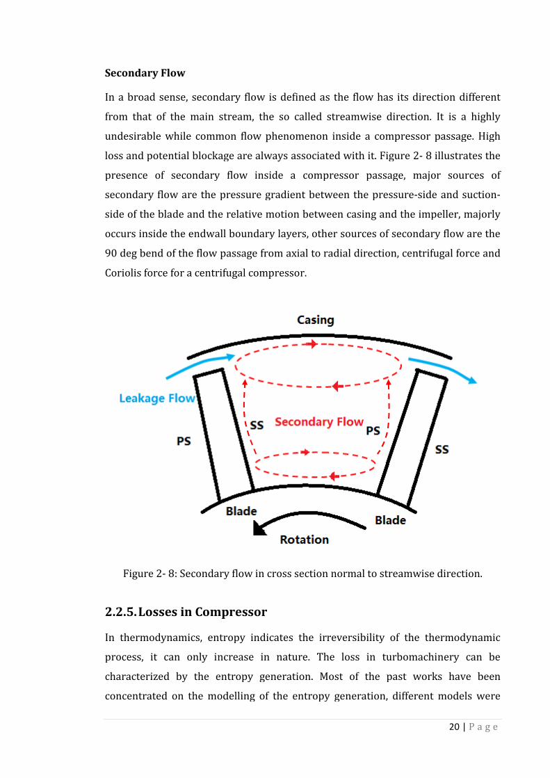
In a broad sense, secondary flow is defined as the flow has its direction different
from that of the main stream,
undesirable while common
loss and potential blockage are
presence of secondary flow in
secondary flow are
side of the blade and the relative motion between
occurs inside the endwall boundary layer
90 deg bend of the flow passage from axial to radial direction
Coriolis force for a centrifugal compressor
Figure 2- 8: Secondary flow in cross section normal to
2.2.5. Losses in Compressor
In thermodynamics, entropy indicates the irreversibility of the thermodynamic
process, it can only increase in nature.
characterized by the entropy generation.
concentrated on the modelling of the entropy generation, different models were
In a broad sense, secondary flow is defined as the flow has its direction different
at of the main stream, the so called streamwise direction.
undesirable while common flow phenomenon inside a compressor passage. Hig
loss and potential blockage are always associated with it. Figure 2
presence of secondary flow inside a compressor passage
the pressure gradient between the pressure
and the relative motion between casing and the impeller
occurs inside the endwall boundary layers, other sources of secondary flow
deg bend of the flow passage from axial to radial direction, centrifugal
for a centrifugal compressor.
: Secondary flow in cross section normal to streamwise direction
Losses in Compressor
In thermodynamics, entropy indicates the irreversibility of the thermodynamic
process, it can only increase in nature. The loss in turbomachinery can be
characterized by the entropy generation. Most of the past wo
concentrated on the modelling of the entropy generation, different models were
20 | P a g e
In a broad sense, secondary flow is defined as the flow has its direction different
so called streamwise direction. It is a highly
inside a compressor passage. High
Figure 2- 8 illustrates the
pressor passage, major sources of
pressure gradient between the pressure-side and suction-
and the impeller, majorly
sources of secondary flow are the
, centrifugal force and
streamwise direction.
In thermodynamics, entropy indicates the irreversibility of the thermodynamic
The loss in turbomachinery can be
Most of the past works have been
concentrated on the modelling of the entropy generation, different models were

21 | P a g e
proposed to evaluate the entropy generation for different situations, such as two-
dimensional boundary layer, fluid mixing, heat transfer and shock wave. A brief
introduction on the major sources of losses is given as follows, some of the
theoretical models are also described to help understanding the physical aspects.
Please refer to Denton (1993) for a comprehensive review.
Entropy Generation
Entropy has been described by Denton (1993) as "smoke", which would be created
where the flow undergoes an irreversible process. It cannot be destroyed and can
only be convected downstream. Entropy can be generated due to different physical
mechanisms, such as viscous effect, heat transfer and nonequilibrium process. In
the case of compressor, the entropy generation due to heat transfer is generally of
negligible level, however, strong coolant flow involved in turbines makes heat
transfer a very significant mechanism of entropy generation and need to be
considered with care. Nonequilibrium process, such as sudden expansion and
shock wave, is very important, but it is not that relevant in the context of current
work. Therefore, only entropy generation due to viscous effect will be discussed
below.
Compressor flow is in fact a wall bounded flow, under the effect of diffusion, the
boundary layer is very thick, thus imply high viscous dissipation involved. An
expression has been derived by Denton (1993) to calculate the total rate of entropy
generation for a two-dimensional boundary layer, as given in Eqn 2-10, the total
rate of entropy generation per unit surface area is directly proportional to the
shear stress, and can be obtained by integration through the boundary layer. From
the calculation with boundary code developed by Cebeci and Carr (1978), Denton
found that much of the entropy was created within the laminar sublayer and the
logarithmic region. For practical use, it is usually more convenient to turn the
entropy generation to a dimensionless dissipation coefficient, as defined in Eqn 2-
11, where Vδ denotes the velocity at the edge of the boundary layer.
S � = ��J K 5ρVJ�s − sN�8dy = K "E τRJdVJN�N� Eqn 2- 10

22 | P a g e
C� = ES TUFV0 Eqn 2- 11
Schlichting (1966) correlated the experimental results and concluded that the
dissipation coefficient for turbulent boundary layers is relatively insensitive to the
state of the boundary layer. Denton (1993) compared the dissipation coefficient
from Schlichting with that from Cebeci and Carr, and drew similar conclusions as
Schlichting, further investigations on the dissipation coefficient for laminar
boundary layer were conducted, it was found that the dissipation coefficient is
sensitive to the state of the boundary layer, and the dissipation coefficient for
laminar boundary layer is much less than that for turbulent boundary layer with Reθ ranging from 300 to 500, which represents the transition region, thus pointed
out the importance of transition prediction in loss estimation.
Another significant source of entropy generation due to viscous effect is the shear
flow, the most common shear flows in turbomachinery are tip leakage flow and
wake. Since there flows are generally turbulent and of high effective viscosity,
what's worse, they are usually highly complex, thus make it very difficult to
quantify the local entropy generation. However, the global entropy generation can
be obtained relatively easily, as described by Denton (1993), a control volume
method can be applied to predict the entropy generation, thus the mixing loss can
be estimated without losing much accuracy, the upstream conditions are assumed
to be known, and the downstream conditions are set to those of far downstream,
for which the flow parameters restore to uniform conditions. A representative
example of such mixing process is given by Denton, it is the mixing of two streams.
With the assumption that one of the two streams is small, a simplified version is
demonstrated by Denton, while the relevant theory was first proposed by Shapiro
(1953). A schematic is shown in Figure 2- 9, where V4 is the cross-stream velocity,
and α denotes the cross-stream angle. The entropy generated in this process can be
expressed as Eqn 2-12 (for main stream), where the subscript c, m and t denote the
cross-stream, main stream and stagnation condition respectively. C� denotes the
specific heat at constant pressure, M denotes the Mach number. A simplified
expression can be obtained if the two streams have the same stagnation
temperature, as Eqn 2-13. Eqn 2-12 and Eqn 2-13 are valid for both constant
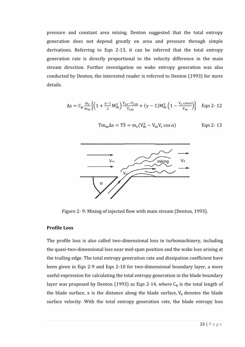
23 | P a g e
pressure and constant area mixing. Denton suggested that the total entropy
generation does not depend greatly on area and pressure through simple
derivations. Referring to Eqn 2-13, it can be inferred that the total entropy
generation rate is directly proportional to the velocity difference in the main
stream direction. Further investigation on wake entropy generation was also
conducted by Denton, the interested reader is referred to Denton (1993) for more
details.
∆s = C� �=�W XY1 + Z#"� M�� \ E&,=#E&,WE&,W + �γ − 1�M�� Y1 − F= 4^- _FW \` Eqn 2- 12
Tm�∆s = TS = m4�V�� − V�V4 cos α� Eqn 2- 13
Figure 2- 9: Mixing of injected flow with main stream (Denton, 1993).
Profile Loss
The profile loss is also called two-dimensional loss in turbomachinery, including
the quasi-two-dimensional loss near mid-span position and the wake loss arising at
the trailing edge. The total entropy generation rate and dissipation coefficient have
been given in Eqn 2-9 and Eqn 2-10 for two-dimensional boundary layer, a more
useful expression for calculating the total entropy generation in the blade boundary
layer was proposed by Denton (1993) as Eqn 2-14, where C� is the total length of
the blade surface, x is the distance along the blade surface, V� denotes the blade
surface velocity. With the total entropy generation rate, the blade entropy loss
24 | P a g e
coefficient can be defined as Eqn 2-15, the inlet velocity is selected as the reference
velocity.
S = ∑ C� K IfUFg0E d�x C�⁄ �"� Eqn 2- 14
ξ� = �ES� Flmn' Eqn 2- 15
Combining Eqn 2-14 and Eqn 2-15, the entropy loss coefficient can be related to the
surface velocity distribution and dissipation coefficient as Eqn 2-16, where p
denotes the pitch. With the knowledge of surface velocity distribution and
dissipation coefficient, it is possible to estimate the blade entropy loss.
ξ- = 2 ∑ Io� 4^- _lmn K C� Y FgFlmn\� d�x C�⁄ �"� Eqn 2- 16
Referring to Eqn 2-16, it is noted that the entropy loss is directly proportional to
the surface velocity distribution and the dissipation coefficient, thus more severe
entropy loss seems to happen at the blade suction side due to relatively higher
surface velocity distribution and much larger extent of turbulent boundary layer.
The effect of Reynolds number and surface roughness on the two-dimensional
boundary layer loss is very complicated, in the laminar regime, the loss increases
significantly with the decrease in Reynolds number due to the high dissipation
coefficient (ReC < 300�, in the transition regime, the loss is mostly dependent on
the surface velocity distribution, even the general trend is difficult to determine. In
turbulent regime, the loss decreases with the increase in Reynolds number for very
smooth blade, the effect of surface roughness is very significant in terms of
increasing the loss. Koch and Smith (1976) conducted a detailed calculation on the
loss in an axial compressor, and concluded that the loss increases significantly with
the increase in surface roughness under high Reynolds number condition.
Wake loss accounts for a significant part of total profile loss. An expression for
wake entropy loss coefficient is derived by Denton as Eqn 2-17, where C�� is the

25 | P a g e
base pressure coefficient. The first term on the RHS denotes the loss due to base
pressure acting on the trailing edge and is greatly affected by the trailing edge
thickness, in the case of impeller with blunt trailing edge, it is obvious that the base
pressure contributes significantly to the wake loss. The second term represents the
mixing loss of the boundary layer before the trailing edge, and the last term
represents the loss due to the boundary layer blockage effect at the trailing edge.
ξs = I%o�s + �Cs + YN∗u�s \� Eqn 2- 17
Tip Leakage Loss
As described previously, the tip leakage loss is the product of tip leakage flow,
which is induced due to the presence of pressure gradient at pressure-side and
suction-side. Referring to Figure 2- 6, in the case of thick blade, the tip leakage flow
mixes out inside the tip clearance, and consequently, the static pressure is
increased as well as the entropy, on the other hand, if the blade is thin, the static
pressure recovery is unlikely to happen inside the tip clearance, mixing occurs near
the suction side corner. The difference in mixing process may give rise to different
entropy generation, Storer (1991) found that most of the entropy generation
occurs just near the point of leakage. Denton (1993) derived an expression for
calculating tip leakage entropy loss coefficient for unshrouded blades with the
assumption of incompressible flow, as given in Eqn 2-18, where Cv is the discharge
coefficient, g is the tip clearance height, C is the chord length, h is the blade span, V-
and V- denotes the suction-side and pressure-side velocity respectively. Referring
to Eqn 2-18, the tip leakage entropy loss coefficient is directly proportional to the
ratio of tip leakage area to inlet flow area, and greatly affected by the ratio of
suction-side velocity to inlet velocity. Both increased tip leakage area and high
suction-side velocity would result in higher tip leakage loss.
ξ1 = �IwxIy� 4^- _lmn K Y F.Flmn\� Y1 − F%F.\ z$1 − YF%F.\�) �{I"� Eqn 2- 18

26 | P a g e
In fact, the effects of centrifugal force and Coriolis force have not been explicitly
considered in Denton's derivation, however, they can be taken into account
through correction on discharge coefficient Cv, which can be measured either from
experimental or numerical simulation.
Endwall Loss
The endwall loss is the loss arising from the hub and casing boundary layer, and
primarily occurs due to the endwall boundary layer separation, as well as very high
speed flow. As described previously, secondary flow is common inside the
compressor, and it tends to convect the low momentum fluid towards the corner
and thus prompt potential separation. High speed flow commonly exists just before
the diffuser, thus cause high endwall loss, Denton (1993) discussed that the
endwall loss is high at the radial part of the casing near the impeller outlet and
inside the diffuser for a centrifugal compressor with unshrouded impeller, while
for the shrouded impeller centrifugal compressor, the endwall loss is relatively
high at the axial part of the casing. In a small size centrifugal compressor, strong
interaction exists between the aforementioned tip leakage flow and the endwall
boundary layer flow, in general, high loss is generated from the interaction,
however, as stated by Storer (1991), tip leakage flow can be beneficial, he showed
that tip leakage flow could help re-energizing the near separation boundary layer at
the suction-side casing corner, and thus prevent the corner separation and reduce
the potential loss. The endwall loss is strongly affected by the incoming boundary
layer and the geometry, as a result, it is very difficult to predict the endwall loss
reliably with any theoretical model.
2.3. Existing Works on Centrifugal Compressor
Generally, there are three different approaches for investigating the centrifugal
compressor, theoretical approach, experimental approach and numerical approach
respectively. Theoretical approach is the most fundamental method, starting with
the basic thermodynamic and fluid dynamic principles to construct a model, which
could represent the real physics as much as possible, general assumptions are
usually made according to the specific problem. Once the model has been

27 | P a g e
constructed, the prediction can be made in very short time, however, for most of
the time, it is heuristic and empirical, rather than mathematical, the models are
mostly based on 1D and 2D assumptions, it is too ideal to take into account the flow
features such as vortex interaction, unsteadiness and etc, the whole picture of
physical mechanism inside a centrifugal compressor is still far from complete.
Experimental approach, as one of the basic tools, is essential to the development of
centrifugal compressor, it has been applied historically and widely to investigating
the performance, flow behaviour and understanding the physics involved, however,
it has been used as a evaluation tool rather than a design tool for most of the time.
Theoretical and experimental approaches for compressor performance evaluation
are acceptable and essential, however, computational modelling is becoming more
critical in the turbomachinery design phase, in certain cases, theoretical approach
cannot provide accurate enough prediction, experiments are expensive and time-
consuming, conversely, computational modelling could be done in relatively short
time and provides more details about the flow field, thus reduces the design cycle,
cost and helps improving the design. It is well known that the computational
modelling is not valid without the support from related experiments, so it is always
applied to complement experimental and theoretical approaches.
Early experiment on centrifugal compressor flow field was very difficult due to the
unavailability of proper instruments, it was not until the end of 1950s that a
representative experiment was conducted by Acosta and Bowerman (1957) thanks
to the development of instruments, rotating pressure probe was employed to
measure the flow field inside four low backsweep(β2=23.5o) 2D impeller and one
low backsweep(β2=17o) 3D impeller. Static pressure distribution, relative velocity
and relative total pressure loss have been obtained, a high loss region was
observed to exist at the suction side shroud corner. The 3D impeller was noted to
have better inflow condition, this may due to design of inducer section on 3D
impeller, the flow can match the blade smoothly.
Experimental investigations led Dean and Senoo (1960) to the well known "jet-
wake structure" model, the flow discharge from the impeller outlet was observed
to be unsteady and axially asymmetric. A theory was proposed based on the
simplified model, the theoretical result was shown to be consistent with the

28 | P a g e
measurements. They believed that the "jet-wake structure" generally mixed out
rather quickly and restore the uniform flow condition. Further investigation has
been conducted by Eckardt (1975), who employed the Laser Anemometer (LA) to
take measurements of flow field inside the Eckardt impeller, it was found that
separation occurred at the suction-side shroud corner 50% chord position, and the
separated region grew towards the impeller outlet, occupied about 20% of the
passage cross-section at 70% chord position, and continued growing to 35% of the
passage cross-section at 90% chord position, however, the separated flow only
account for 15% of the total mass flow rate. Highly non-uniform flow with regions
of low momentum and high momentum fluids were observed at the impeller outlet,
thus confirmed the existence of "jet-wake structure". Later, Johnson and Moore
(1980) investigated the effect of secondary flow on the convection of low rotary
stagnation pressure (p∗ = p + 1 2⁄ ρW� − 1 2⁄ ω�r�) fluid and the formation of
wake at the suction-side shroud corner, measurements on relative velocities and
rotary stagnation pressures were taken on five cross-sectional planes between the
inlet and outlet of the impeller, it was concluded that the convection of low rotary
stagnation pressure fluid is critical to the formation of "jet-wake structure" at the
impeller outlet.
Krain (1988) studied the flow field inside a newly design backswept impeller using
Laser-2-Focus (L2F) technique, the distortion of through-flow pattern and the
formation of secondary flow were attributed to the presence swirling flow inside
the impeller. Separation was observed at the pressure-side near 50% chord
position, and grew towards downstream, then the separated fluid moved to the
middle of the passage at 70% chord position and occupied half of the passage cross
section, and then the flow smoothed near the impeller outlet, "jet-wake structure"
was clearly identified, however, it was different from the widely accepted classical
"jet-wake structure" observed by Dean and Senoo (1960). A Low Speed Centrifugal
Compressor (LSCC) was designed at NASA to duplicate the important features of
high speed subsonic centrifugal compressor in a large low speed substitute, thus
enables the flow field measurements with LA. Hathaway et al. (1993) conducted
detailed experiments and numerical simulation on LSCC, it was found that the low
momentum fluid near the blade surface migrated towards to blade tip, and

29 | P a g e
entrained in the tip clearance flow, and then this fluid is transported towards the
pressure-side/shroud corner, finally, contributed to the formation of through-flow
wake, which mixed out slowly, as a result, two different wakes were observed in
the vaneless space, through-flow wake and viscous blade wake respectively.
Tip leakage flow plays an important role in the performance and stability of the
centrifugal compressor, Pampreen (1973) discussed the design consideration for
small centrifugal compressors, performance data were collected for 6 different
centrifugal compressors to investigate the effect of tip clearance and Reynolds
number, it was found that the correlation between the compressor performance
and the tip clearance was rather irregular, however, on average, the compressor
performance deteriorated by 3% with the increase in tip clearance by 10%, and tip
clearance effect is more prominent for small centrifugal compressor compared to
Reynolds number effect. Later, Klassen, Wood and Schumann (1977a; 1977b)
confirmed the detrimental effect of tip clearance on the centrifugal compressor
performance through experiments on two different high pressure ratio centrifugal
compressor, it was concluded that the efficiency drops as the increase in tip
clearance for all tested rotational speed and mass flow rate. Syed, Ma and Yang
(2006) conducted numerical simulation on a unshrouded impeller centrifugal
compressor to investigate the effect of tip clearance, which was varied from 0mm
to 1mm. The efficiency was found to be the highest if there was not tip clearance,
and worst with the largest tip clearance, and it was also found that the impeller and
diffuser were affected differently by the tip clearance, the impeller efficiency
peaked at smaller tip clearance, while diffuser efficiency peaked at larger tip
clearance.
Mashimo, Watanabe and Ariga (1979) conducted detailed experiments on the tip
leakage flow induced loss in a centrifugal compressor. Tip clearance, Reynolds
number and operation conditions were varied independently, it was found that
centrifugal compressor operating at large mass flow rate tends to have more
efficiency drop due to the increase in tip clearance, and tip leakage loss is higher if
the Reynolds number is increased, however, the effect was found to be minor. The
underlying reason may be that the impeller operating at higher mass flow rate will
experience higher blade loading, thus cause higher pressure gradient between the

30 | P a g e
blade pressure-side and suction-side. Similar conclusion has also been made by
Senoo and Ishida (1987), who modified their original theory on the tip clearance
loss of centrifugal impellers to include the variation of slip angle due to tip leakage
flow, and validated with the experimental results in literature, good agreement was
achieved. The efficiency was found to be less sensitive to the tip leakage flow for
small flow rate centrifugal impeller, so was the high pressure ratio compressor at
reduced shaft speed. Plamer and Waterman (1995) designed a two-stage high
pressure ratio centrifugal compressor. Two different impellers were tested, one
with 16 main and 16 splitter blades, and the other with 19 main and 19 splitter
blade. The former tends to have relatively uniform meridional blade loading, while
the latter has reduced loading near the blade trailing edge. It was found that the
efficiency was relatively less sensitive to the tip clearance for the reduced loading
impeller.
Ishida and Senoo (1981) measured the pressure distribution along the shroud for
three types of centrifugal impeller at seven different tip clearances each, tip
clearance ratio and static pressure rise due to the reduction in relative velocity are
directly related to the tip clearance loss, it was inferred that the compressor
performance could be improved by reducing the tip clearance at the leading edge,
where the reduction in relative velocity is significant. To investigate the effect of tip
clearance ratio on the input power, velocity distribution, relative flow angle, further
experiments have been conducted by Ishida, Senoo and Ueki (1990) on two types
of unshrouded centrifugal impellers at four different tip clearance each, one is
radial impeller and the other is backward-leaning impeller, it was found that, for
radial impeller, the input work, velocity distribution and relative flow angle were
hardly changed at different tip clearances, while for the backward-leaning impeller,
the input power and relative flow angle were reduced if the tip clearance was
increased, the velocity distribution was not affected noticeably.
Farge, Johnson and Maksound (1989) studied the tip leakage flow inside an
shrouded impeller with an internal tip clearance between the shroud and the blade
tips. They found that the static pressure distribution is almost unaltered with the
presence of tip clearance. The low momentum fluid from the suction side surface
and tip leakage flow accumulated at the suction-side/shroud corner and

31 | P a g e
contributed to the formation of wake, which mitigated to the middle of the shroud
at the impeller outlet due to the effect of tip leakage flow. While Liu, Ping and
Zangeneh (2013) conducted numerical simulation on the Eckardt impeller to
investigate the effect of tip leakage flow, three different tip clearance size
configurations were examined, 0%, 2.9% and 4.96% of exit width respectively. It
was found that there is clear correlation between the blade loading and tip leakage
flow distribution, the magnitude of the blade loading was reduced with the increase
of tip clearance size, while the shape of the blade loading curve did not change
greatly. A small amount of loss occurred inside the tip clearance, instead, much of
the loss happened due to the formation of tip leakage vortex.
Schleer, Song and Abhari (2008) investigated the effect of large tip clearance on the
onset of instability inside a highly-loaded centrifugal compressor, time-resolved
static pressure measurements were taken along the shroud surface for two
different tip clearance configurations, tip leakage vortex was identified as a region
of high pressure deviation originating from the leading edge, they found that the
trajectory of this vortex was strongly affected by the mass flow rate and the tip
clearance size. The tip leakage vortex tended to move upstream when the mass
flow rate was reduced, and touched the blade pressure-side at sufficiently low mass
flow rate, further reducing the mass flow rate caused the tip leakage vortex
trajectory to be perpendicular to the rotation axis, and initialized the inlet tip
recirculation, and ultimately led to the disappearance of tip leakage vortex and
rotating stall inside the diffuser. It seems that there is a relation between the tip
leakage flow and the rotating stall inception, Tomita et al. (2013) studied two
centrifugal compressor with different operation range widths using both
experimental and computational methods. It was found that, in the case of narrow
operation range compressor, the amplitude of blade passing pressure fluctuation
decreased rapidly as the inlet mass flow rate was reduced, while for the
counterpart, the amplitude of blade passing pressure fluctuation decreased
gradually. Blockage due to tip leakage vortex breakdown was observed for the
latter only, it was concluded that the blockage was actually beneficial, it worked to
stabilize the flow field, and delayed the occurrence of rotating stall.
32 | P a g e
Another very important phenomenon inside a centrifugal compressor with vaned
diffuser is the impeller-diffuser interaction. The unsteadiness induced due to the
diffuser vanes would distort the certain potion of the impeller flow field, and cause
fluctuating forces on the impeller blade; at the same time, the wake shedding from
the impeller blade would affect the diffuser flow field. Early work on the potential
effect of diffuser vane on the impeller flow field was conducted by lino and Kasai
(1985). The most critical parameter determining the impeller-diffuser interaction
is the radial spacing, as pointed out by Rodgers (1982), Clements and Artt (1989),
Gottfreid and Fleeter (2002), the existence of an optimum radial spacing for peak
performance is also identified.
More detailed flow measurements and numerical simulation would help to reveal
the flow features of the impeller-diffuser interaction. Arndt et al. (1990)
investigated the impeller-diffuser interaction by conducting experiment on a
centrifugal compressor, with two-dimensional impeller and vaned diffuser. The
flow coefficient and number of diffuser blade were varied, as well as the gap
between the impeller blade trailing edge and the diffuser blade leading edge. It was
observed that large pressure fluctuations occurred in both diffuser and impeller
and were the same order of magnitude as the total pressure across the compressor.
For diffuser, the largest pressure fluctuation occurred on the suction-side near the
blade leading edge, while the largest pressure fluctuation occurred at the blade
trailing edge for impeller. The flow coefficient was found to have opposite effects
for impeller and diffuser, the increase in flow coefficient tends to cause increase in
impeller pressure fluctuation and reduction in diffuser pressure fluctuation. It was
also found that the increase in diffuser blade would reduce the impeller pressure
fluctuation significantly.
Ubaldi et al. (1996) made detailed flow measurements in the so called ERCOFTAC
centrifugal compressor to investigate the influence of diffuser vanes induced
unsteadiness on the impeller flow. Local defects of radial velocity and pressure
fluctuations were observed due to the presence of diffuser vanes. The periodic
interaction between the diffuser vane induced unsteadiness and the
nonuniformities of impeller relative flow gives rise to the unsteady work transfer
(implied from Euler work equation) and local reverse flow. The diffuser vane

33 | P a g e
induced pressure fluctuations actually affect the pressure level in the whole
impeller. Recently, numerical simulation was conducted on the ERCOFTAC
centrifugal compressor by Petit and Nilsson (2013), comparison was made
between the computed results and experimental data, good agreement was
achieved.
Shum, Tan and Cumpsty (2000) found that larger viscous loss is associated with tip
leakage flow with the presence of impeller-diffuser interaction using numerical
simulation, the effects of impeller-diffuser interaction on the flow field at impeller
outlet can be summarized as reduced blockage, reduced slip and increased loss.
The reduction in radial spacing could help to reduce the blockage and slip, however,
too small the radial spacing would bring large viscous loss and overweigh the
benefits. It is thus proved the existence of an optimum radial spacing for peak
performance. They also found that the effect of impeller-diffuser interaction on
impeller is much more significant than that on diffuser. They concluded that the
beneficial effects of impeller-diffuser interaction are mainly attributed to the
reduced blockage and reduced slip associated with tip leakage flow.
Ziegler, Gallus and Niehuis (2003) investigated the effect of impeller-diffuser
interaction on the diffuser performance, the radial spacing was varied between 4
and 18%. They found that the reduction in radial spacing results in slightly increase
in the impeller work input, while the diffuser performance is improved in terms of
pressure recovery coefficient and total pressure loss coefficient. They attributed
the improved diffuser performance to the unloading of the highly loaded vane
pressure-side, which tends to bring more homogeneous flow field. Further study
has been conducted by Boncinelli et al. (2007) numerically, two centrifugal
compressors with different radial spacing was simulated with both steady and
unsteady simulation. The computed results were validated against the
experimental data from Ziegler, Gallus and Niehuis. They found that the
unsteadiness from the impeller-diffuser interaction could actually bring the high
energy fluid at the vane suction-side to the pressure-side, thus unloads the highly
loaded pressure-side and suppresses the pressure-side separation, as a result, the
total pressure loss is reduced.
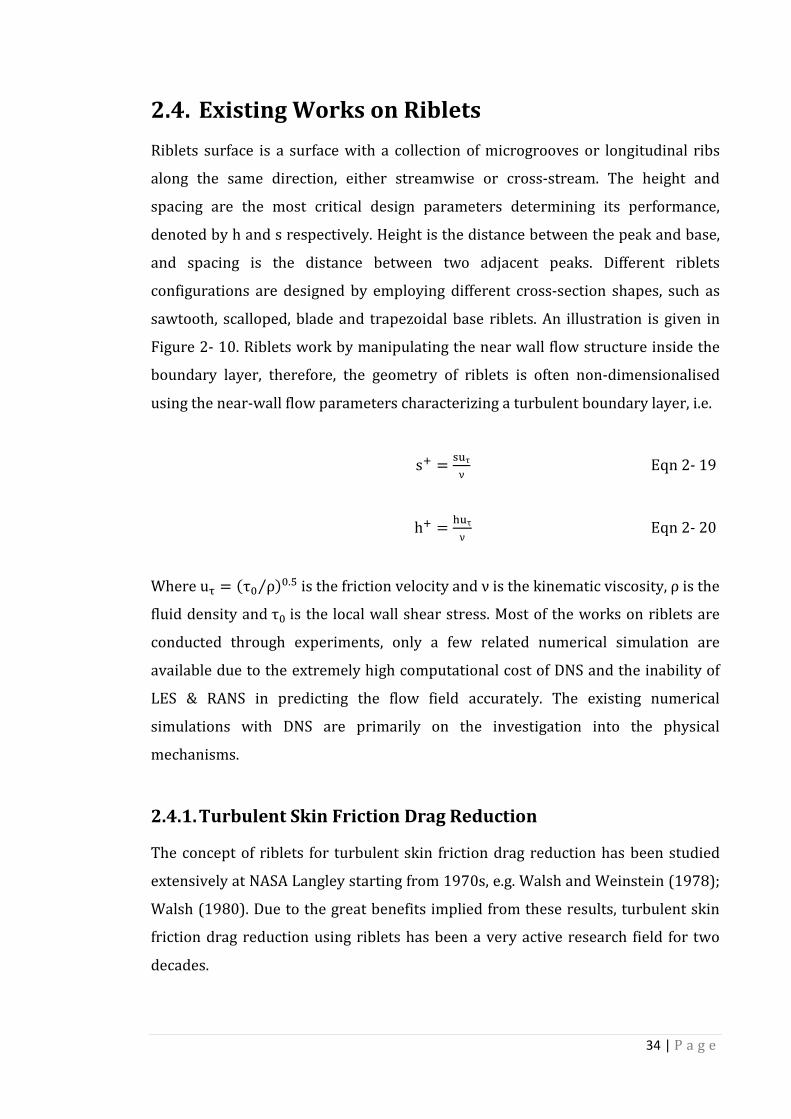
34 | P a g e
2.4. Existing Works on Riblets
Riblets surface is a surface with a collection of microgrooves or longitudinal ribs
along the same direction, either streamwise or cross-stream. The height and
spacing are the most critical design parameters determining its performance,
denoted by h and s respectively. Height is the distance between the peak and base,
and spacing is the distance between two adjacent peaks. Different riblets
configurations are designed by employing different cross-section shapes, such as
sawtooth, scalloped, blade and trapezoidal base riblets. An illustration is given in
Figure 2- 10. Riblets work by manipulating the near wall flow structure inside the
boundary layer, therefore, the geometry of riblets is often non-dimensionalised
using the near-wall flow parameters characterizing a turbulent boundary layer, i.e.
su = -3τ
ν Eqn 2- 19
hu = y3τ
ν Eqn 2- 20
Where u� = �τ� ρ⁄ ��.� is the friction velocity and ν is the kinematic viscosity, ρ is the
fluid density and τ� is the local wall shear stress. Most of the works on riblets are
conducted through experiments, only a few related numerical simulation are
available due to the extremely high computational cost of DNS and the inability of
LES & RANS in predicting the flow field accurately. The existing numerical
simulations with DNS are primarily on the investigation into the physical
mechanisms.
2.4.1. Turbulent Skin Friction Drag Reduction
The concept of riblets for turbulent skin friction drag reduction has been studied
extensively at NASA Langley starting from 1970s, e.g. Walsh and Weinstein (1978);
Walsh (1980). Due to the great benefits implied from these results, turbulent skin
friction drag reduction using riblets has been a very active research field for two
decades.
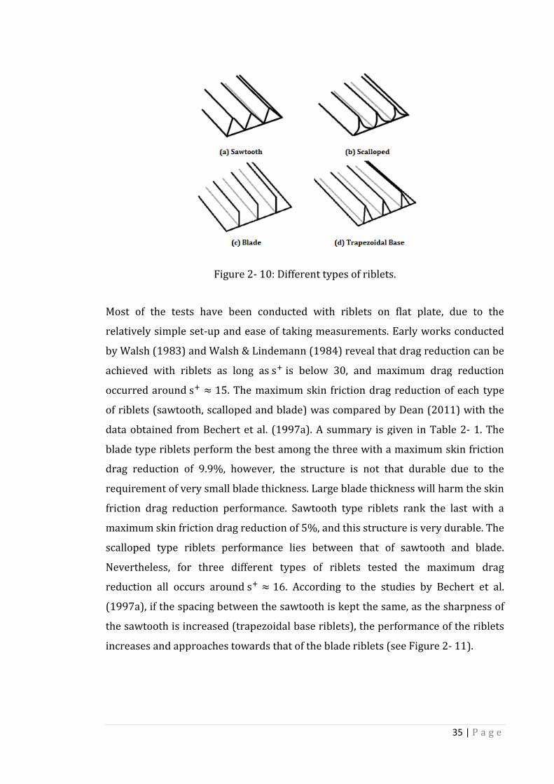
Most of the tests have been conducted with riblets on flat plate, due to the
relatively simple set
by Walsh (1983) and Walsh & Linde
achieved with riblet
occurred around su
of riblets (sawtooth, scalloped and blade)
data obtained from Bechert et al
blade type riblets perform the best among the three with a maximum skin friction
drag reduction of 9.9%, however
requirement of very small blade thickness. Large blade thickness will harm the skin
friction drag reduction performance. Sawtooth type riblets rank the last with a
maximum skin friction
scalloped type riblets performance lies between that of sawtooth and blade.
Nevertheless, for three different types of riblets tested the maximum drag
reduction all occurs around
(1997a), if the spacing between the sawtooth is kept the same, as the sharpness of
the sawtooth is increased
increases and approaches towards that of the blade riblets
Figure 2- 10: Different types of riblets.
Most of the tests have been conducted with riblets on flat plate, due to the
relatively simple set-up and ease of taking measurements. Early
1983) and Walsh & Lindemann (1984) reveal that drag reduction can be
achieved with riblets as long as su is below 30, and maximum drag reduction
� 15. The maximum skin friction drag reduction of
sawtooth, scalloped and blade) was compared by Dean (2011)
data obtained from Bechert et al. (1997a). A summary is given in
blade type riblets perform the best among the three with a maximum skin friction
reduction of 9.9%, however, the structure is not that durable due to the
requirement of very small blade thickness. Large blade thickness will harm the skin
reduction performance. Sawtooth type riblets rank the last with a
maximum skin friction drag reduction of 5%, and this structure is very durable.
ped type riblets performance lies between that of sawtooth and blade.
Nevertheless, for three different types of riblets tested the maximum drag
reduction all occurs around su � 16. According to the studies by
), if the spacing between the sawtooth is kept the same, as the sharpness of
the sawtooth is increased (trapezoidal base riblets), the performance of the riblets
increases and approaches towards that of the blade riblets (see
35 | P a g e
Most of the tests have been conducted with riblets on flat plate, due to the
Early works conducted
(1984) reveal that drag reduction can be
is below 30, and maximum drag reduction
reduction of each type
compared by Dean (2011) with the
given in Table 2- 1. The
blade type riblets perform the best among the three with a maximum skin friction
, the structure is not that durable due to the
requirement of very small blade thickness. Large blade thickness will harm the skin
reduction performance. Sawtooth type riblets rank the last with a
nd this structure is very durable. The
ped type riblets performance lies between that of sawtooth and blade.
Nevertheless, for three different types of riblets tested the maximum drag
e studies by Bechert et al.
), if the spacing between the sawtooth is kept the same, as the sharpness of
, the performance of the riblets
(see Figure 2- 11).

Table 2- 1: Comparison of optimum geometry of different riblets
Wang et al. (2008) also studied the performance of sawtooth riblets and
trapezoidal tip riblets with slight variations in their geometry
water flow at a speed of 1.54 m/s. Particle Image Velocimetry
take measurements of the near wall velocity distribution of both grooved surface
and smooth surface. The
empirical formula were used to calculate the local skin friction coefficient. The
results are shown in
could achieve total drag reduction, it is also noted that with a smaller spacing s, the
drag reduction performance is improved. They concluded that the peak geometry
has a great effect on the dra
riblets, the total drag increased due to a larger wetted area. It is obvious that the
non-dimensional spacing
Figure 2- 11: Drag reduction performance of various rib
1997a).
: Comparison of optimum geometry of different riblets
(2008) also studied the performance of sawtooth riblets and
riblets with slight variations in their geometry
water flow at a speed of 1.54 m/s. Particle Image Velocimetry
take measurements of the near wall velocity distribution of both grooved surface
and smooth surface. The loss of momentum method and Ludwieg & Tillman
empirical formula were used to calculate the local skin friction coefficient. The
in Table 2- 3. It is observed that the first three configurations
could achieve total drag reduction, it is also noted that with a smaller spacing s, the
drag reduction performance is improved. They concluded that the peak geometry
has a great effect on the drag reduction performance. In the case of trapezoidal tip
, the total drag increased due to a larger wetted area. It is obvious that the
dimensional spacing su and the effectiveness of riblets are closely correlated.
: Drag reduction performance of various rib geometries (Bechert et al.,
36 | P a g e
: Comparison of optimum geometry of different riblets (Dean, 2011).
(2008) also studied the performance of sawtooth riblets and
riblets with slight variations in their geometry (see Table 2- 2) in a
water flow at a speed of 1.54 m/s. Particle Image Velocimetry (PIV) was used to
take measurements of the near wall velocity distribution of both grooved surface
loss of momentum method and Ludwieg & Tillman
empirical formula were used to calculate the local skin friction coefficient. The
. It is observed that the first three configurations
could achieve total drag reduction, it is also noted that with a smaller spacing s, the
drag reduction performance is improved. They concluded that the peak geometry
the case of trapezoidal tip
, the total drag increased due to a larger wetted area. It is obvious that the
and the effectiveness of riblets are closely correlated.
geometries (Bechert et al.,
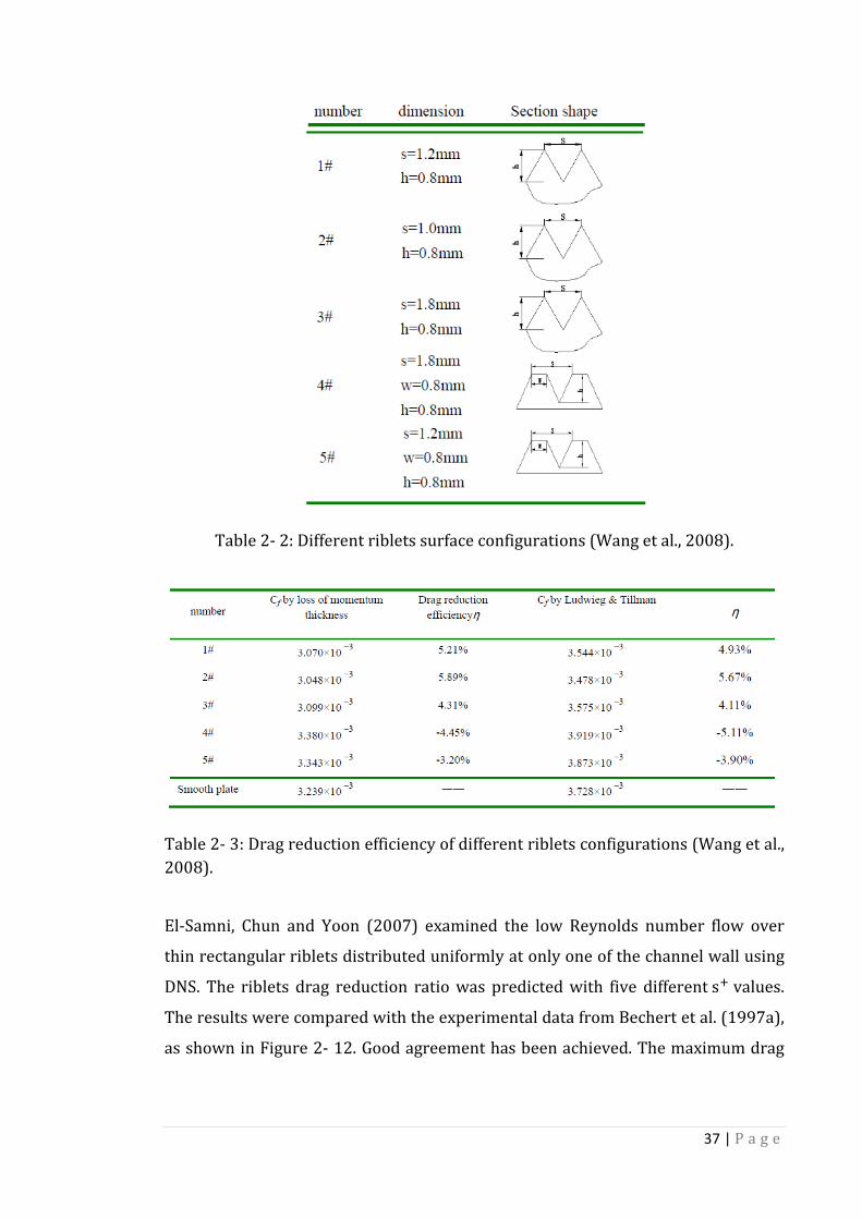
37 | P a g e
Table 2- 2: Different riblets surface configurations (Wang et al., 2008).
Table 2- 3: Drag reduction efficiency of different riblets configurations (Wang et al.,
2008).
El-Samni, Chun and Yoon (2007) examined the low Reynolds number flow over
thin rectangular riblets distributed uniformly at only one of the channel wall using
DNS. The riblets drag reduction ratio was predicted with five different su values.
The results were compared with the experimental data from Bechert et al. (1997a),
as shown in Figure 2- 12. Good agreement has been achieved. The maximum drag
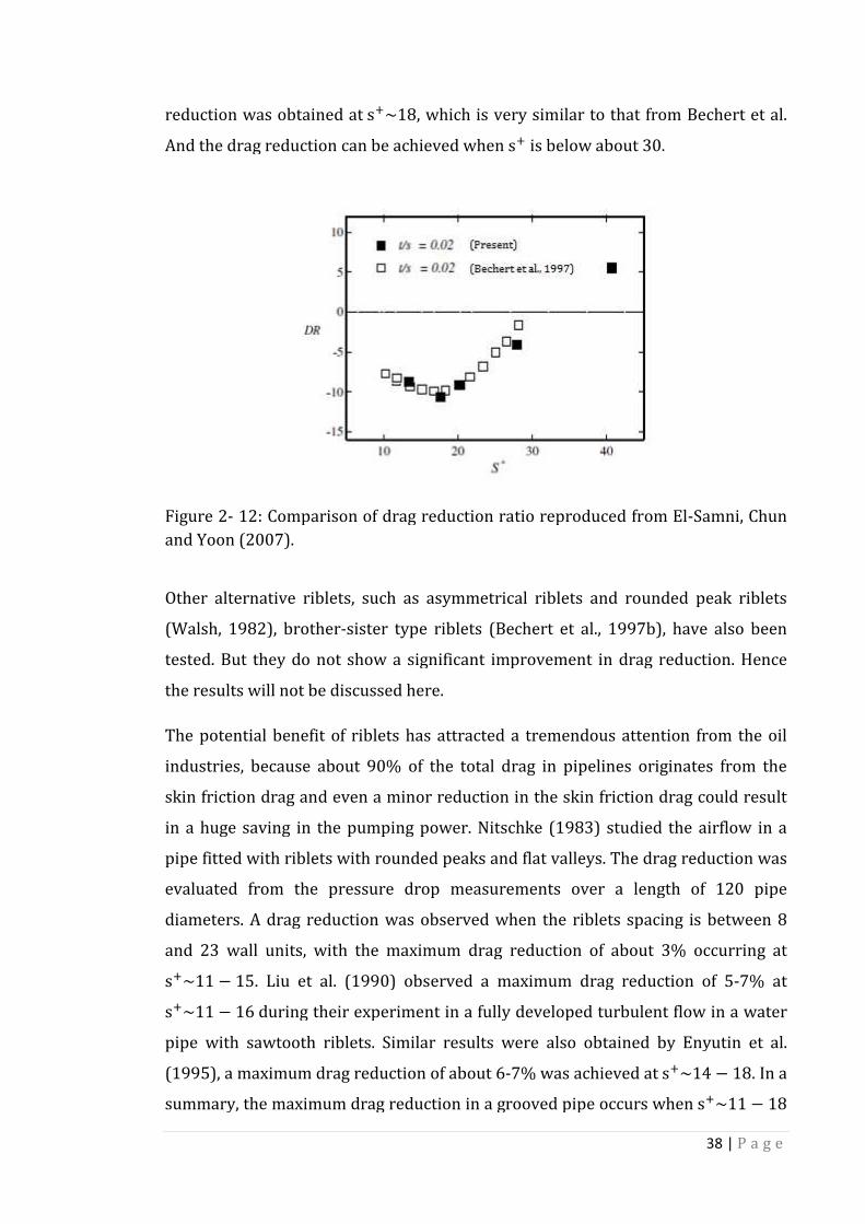
reduction was obtained at
And the drag reduction can be achieved when
Figure 2- 12: Comparison of drag reduction ratio reproduced from El
and Yoon (2007).
Other alternative riblets, such as asymmetrical riblets and rounded peak riblets
(Walsh, 1982), brothe
tested. But they do not show a significant improvement in drag reduction. Hence
the results will not be discussed here.
The potential benefit of riblets has attracted a tremendous attention from the oil
industries, because about 90%
skin friction drag and even a minor reduction in the skin friction
in a huge saving in the pumping power. Nitschke (1983) studied the airflow in a
pipe fitted with riblets with rounded
evaluated from the pressure drop measurements over a length of 120 pipe
diameters. A drag reduction was observed when the riblets spacing is between 8
and 23 wall units, with the maximum drag reduction of abou
su~11 7 15. Liu et al. (1990) observed a maximum drag reduction of 5
su~11 7 16 during their experiment in a fully developed turbulent flow in a water
pipe with sawtooth
(1995), a maximum drag reduction of about 6
summary, the maximum drag reduction in a grooved pipe occurs when
reduction was obtained at su~18, which is very similar to that from Bechert et al
And the drag reduction can be achieved when su is below about 30.
: Comparison of drag reduction ratio reproduced from El
Other alternative riblets, such as asymmetrical riblets and rounded peak riblets
(Walsh, 1982), brother-sister type riblets (Bechert et al., 1997
tested. But they do not show a significant improvement in drag reduction. Hence
the results will not be discussed here.
The potential benefit of riblets has attracted a tremendous attention from the oil
industries, because about 90% of the total drag in pipelines originates from the
and even a minor reduction in the skin friction
in a huge saving in the pumping power. Nitschke (1983) studied the airflow in a
pipe fitted with riblets with rounded peaks and flat valleys. The drag reduction
evaluated from the pressure drop measurements over a length of 120 pipe
diameters. A drag reduction was observed when the riblets spacing is between 8
and 23 wall units, with the maximum drag reduction of abou
. Liu et al. (1990) observed a maximum drag reduction of 5
during their experiment in a fully developed turbulent flow in a water
sawtooth riblets. Similar results were also obtained by Enyutin et al.
5), a maximum drag reduction of about 6-7% was achieved at
summary, the maximum drag reduction in a grooved pipe occurs when
38 | P a g e
ilar to that from Bechert et al.
is below about 30.
: Comparison of drag reduction ratio reproduced from El-Samni, Chun
Other alternative riblets, such as asymmetrical riblets and rounded peak riblets
1997b), have also been
tested. But they do not show a significant improvement in drag reduction. Hence
The potential benefit of riblets has attracted a tremendous attention from the oil
of the total drag in pipelines originates from the
and even a minor reduction in the skin friction drag could result
in a huge saving in the pumping power. Nitschke (1983) studied the airflow in a
peaks and flat valleys. The drag reduction was
evaluated from the pressure drop measurements over a length of 120 pipe
diameters. A drag reduction was observed when the riblets spacing is between 8
and 23 wall units, with the maximum drag reduction of about 3% occurring at
. Liu et al. (1990) observed a maximum drag reduction of 5-7% at
during their experiment in a fully developed turbulent flow in a water
Similar results were also obtained by Enyutin et al.
7% was achieved at su~14 7 18. In a
summary, the maximum drag reduction in a grooved pipe occurs when su~11 7 18
39 | P a g e
and the variation in the optimal su may be attributed to the measurement
uncertainties.
The effects of riblets on the performance of compressor have also been investigated
by only a few researchers. Boese and Fottner (2002) conducted an experimental
investigation of the loss behaviour of a highly loaded compressor cascade under
the effects of riblets. Three riblets configurations with different sizes were first
tested, a optimum size for riblets was obtained with the pressure measurements.
Then a detailed flow visualization was conducted on the optimized riblets
(su = 2hu), which are actually trapezoidal base riblets. The results show that the
riblets mainly affect the suction-side boundary layer behaviour, a reduction in loss
coefficient of 6-8% was achieved when hu ≈ 9, and loss increases when hu is above
20. Later, Oehlert and Seume (2006) tested the machined trapezoidal base riblets
fabricated by grinding and laser machining on NACA compressor blades, they found
it was difficult to achieve the required accuracy by machining. A loss reduction
about 3% was achieved by riblets on flat plate, while for compressor blade, only 1.5%
reduction in loss was obtained. Lietmeyer, Oehlert and Seume (2013) conducted
further tests on a NACA 6510 compressor blade with trapezoidal base riblets on
pressure-side or suction-side or both sides. A profile loss reduction of 4% was
obtained with the riblets on the suction-side, while a reduction of 1.01% was
achieved with the riblets on the pressure-side, if riblets are applied on both sides, a
loss reduction of 4.9% was obtained. Investigation of compressor blade under high
pressure-side incidence showed that a loss reduction up to 7.2% was achieved with
riblets on suction-side, this higher reduction was attributed to the elimination of
suction-side separation bubble with riblets. It is noted that the application of riblets
is the most effective when applied to suction-side. However, it should also be noted
that all the riblets applications in compressor as given above are all applied to
cascade only, for which the blades are completely stationary.
The effects of pressure gradient and yaw angle are very important in practical
application, they have been investigated by many researchers. Sundaram et al.
(1996; 1999) tested the effectiveness of riblets in drag reduction on two different
airfoils up to moderate incidence angles in wind tunnels. The Clauser pressure
gradient parameter, β = N∗�� ���J, was used to characterize the level of adverse

40 | P a g e
pressure gradient at various incidence angles. It was concluded that the
effectiveness of riblets increases with the adverse pressure gradient up a certain
value of β, beyond which the effectiveness is reduced, presumably due to the flow
separation on the airfoil upper surface. The yaw angle has a significant effect on the
magnitude of drag reduction. Walsh and Lindemann (1984) showed that at a yaw
angle of 15 deg the maximum drag reduction is only reduced slightly, however,
when the yaw angle increases to 30 deg, no drag reduction was observed. Coustols
(1989) studied the yaw-angle effects with 3M riblets, he observed that the drag
reduction was significantly reduced from 10 to 3% at a yaw angle of 20 deg. He also
found that the drag reduction dropped from 7 to 3% for an axisymmetric body
when the yaw angle increased from 0 deg to 20 deg. Similar conclusions on the
effect of yaw angle have also been drawn by Sundaram et al. (1999).
A lot of work has been undertaken to understand the physical mechanism of riblets
in turbulent skin friction drag reduction. Some hypotheses have been proposed.
However, the physical mechanism is still an open question under extensive
research. It is also possible that different physical mechanisms work together to
make the riblets effective in reducing the turbulent skin friction drag.
Bacher and Smith (1985) pointed out that the flow field above the riblets surface
will look like what is illustrated in Figure 2- 13. Due to the presence of riblets, a
pair of counter rotating secondary vortex was generated between the peaks of
riblets, just above the riblets. This pair of secondary vortices increased the skin
friction drag at the peak of the riblets, but within a limited region. They weaken the
primary streamwise vortex formed during the bursting process, as a result the fluid
flow at the bottom of the riblets is at lower speed, and the skin friction drag
reduction outweighs the increased drag due to the increased wetted area. Choi,
Moin and Kim (1993) studied the turbulent flow over riblets (v-groove) with DNS
to investigate the physical mechanism. They announced that their results are in
good agreement with experimental results. The mean velocity profile shows
upward and downward shifts in the log-law for drag decreasing and drag
increasing cases respectively. They found that the differences in mean velocity and
turbulence quantities are limited to the inner region of the turbulent boundary
layer. In the case of drag reduction configuration, the velocity, vorticity fluctuations

41 | P a g e
and the Reynolds shear stresses above the riblets were reduced. They concluded
that the viscous drag reduction happened to the riblets with small spacing is caused
by the restricted streamwise vortices above the riblets such that only a limited
wetted area is exposed to the high speed fluid. On the contrary, the streamwise
vortices will be located in the riblets valleys for riblets with larger spacing. Similar
physical mechanism has also been proposed by El-Samni, Chun and Yoon (2007).
With reference to Walsh (1982), Walsh (1983) postulated that the riblets act to
reduce the intensity of the near-wall turbulence eruptions rather than reduce the
frequency of eruptions. Choi (1989), on the other hand, proposed that the presence
of riblets will impede the spanwise motion of streamwise vortices, hence disrupt
and weaken the bursting process and result in a skin friction drag reduction. In
contrary, in the case of laminar flow, the skin friction drag will increase due to the
presence of riblets, which increases the wetted area considerably.
Figure 2- 13: Schematic of streamwise vortex interaction with riblets surface via
viscous effects (Bacher and Smith, 1985).
2.4.2. Delay of Laminar-Turbulent Transition
As mentioned previously laminar-turbulent transition is a very important and
extensively studied topic, nonetheless, the physical mechanism involved is still not
fully understood. If the laminar-turbulent transition can be delayed, the direct
benefit is the reduction in skin friction drag. The research into the effect of riblets
42 | P a g e
on laminar-turbulent transition is only conducted by a few researchers. Early
works were done by Kozlov et al. (1990), Neumann & Dinkelacker (1991), the
beneficial effects of riblets on delaying transition were found. A representative
work was conducted by Grek, Kozlov and Titarenko (1996), the effect of riblets on
the three-dimensional nonlinear structure occurring during laminar-turbulent
transition was studied. This nonlinear structure is also called the Λ-structure. They
found that the application of riblets would delay the transformation of Λ-structure
into turbulent spot, thus shifts the transition point downstream. This finding is
quite opposite to the effect of riblets on two-dimensional Tollmien-Schlichting (TS)
waves, for which the disturbance is excited, thus induce early transition. In total,
the riblets would help to stabilize the Λ-structure (nonlinear stage of transition)
and destabilize the TS waves (linear stage of transition). Therefore, special
attention has to be paid to the location of riblets. Further development can be
found in Litvinenko et al. (2006) on the physical mechanism of delaying the
transformation of Λ-structure.
2.5. Discussion
In this chapter, the general performance parameters and different flow phenomena
of centrifugal compressor were introduced, the flow involved is complicated,
distinct features like viscous, highly unsteady, swirling and transitional make it
very difficult to obtain a reliable prediction. The effect of strong curvature,
centrifugal force, Coriolis force and strong interaction further complicate the
situation. The loss mechanisms in compressors were discussed with the help of
theoretical models, it was shown that tip leakage loss is mainly related to the ratio
of tip leakage area to inlet area and the ratio of suction-side velocity to inlet
velocity, in other words, if the inlet condition is fixed, the tip leakage loss will be
higher with larger tip clearance size and higher suction-side velocity. Two-
dimensional profile loss and endwall loss are very similar, they are dependent on
the state of the boundary layer and surface velocity. Wake loss is another kind of
profile loss, it is closely related to the shape of the trailing edge and the state of the
boundary layer. In the case of centrifugal compressor, two-dimensional profile loss
seldom occurs, the blade surface loss is very similar to the endwall loss. In

43 | P a g e
literature, large amount of works have been done on centrifugal compressor, the
flow behaviour varies for different geometries, therefore, it is essential to analyse
the flow field for a different centrifugal compressor. Riblets surface is effective in
reducing the turbulent skin friction drag and delaying laminar-turbulent transition.
The concept of applying riblets to turbulent skin friction drag reduction has been
pursued extensively, trapezoidal base riblets have been found to be the best
considering the drag reduction performance and ease-of-manufacture. The
discussion on riblets will be elaborated in chapter 8, where riblets have been
proposed to reduce the hub endwall loss in Dyson V2 centrifugal compressor.
44 | P a g e
Chapter 3 Turbulence Modelling
Turbulence Modelling
3.1. Introduction
In most cases, it is not generally possible to depict the complete picture of natural
and engineering flow without referring to turbulence theory. A turbulent flow is
characterized by its chaos in both space and time. Osborne Reynolds is probably
most famous for his findings on the difference of laminar and turbulent flows. In
1883, a series of experiments were conducted at the University of Manchester,
coloured dye was steadily injected on the centreline of a pipe in which water was
flowing (the interested reader is referred to the MACE website for a picture of the
experimental apparatus). Reynolds found that the flow pattern was quite stable
and the dye can be clearly identified even far downstream when the flow is at low
speed, as the flow speed was increased, at certain point, the flow pattern
underwent significant changes, the injected dye began to oscillate and mixed out.
Figure 3- 1 presents a sketch of the distinct flow patterns, with which Reynolds
classified the flow into two categories, laminar and turbulent flow respectively. The
onset of the oscillating flow pattern was found to be related to the inertial and
viscous forces, a non-dimensional number called Reynolds number was proposed
to include the inertial and viscous forces, as defined in Eqn 3-1, where ρ denotes
the fluid density, U denotes the fluid velocity, L denotes a length scale (denotes the
pipe diameter here) and μ is the dynamic viscosity.

45 | P a g e
Re = UH�� Eqn 3- 1
For pipe flow, the transition from laminar to turbulent flow could occur in a range
of Reynolds numbers from approximately 2300 to 4000. For the flow to keep the
state of laminar, the Reynolds number should be less than 2300, on the other hand,
if the Reynolds number exceeds 4000, then the flow is turbulent.
Figure 3- 1: Laminar and turbulent flow patterns (Reynolds, 1901).
The nature of turbulence is generally described through the energy cascade
proposed by Richardson (1922), who hypothesized that turbulent flow contains
lots of eddies with different sizes, eddies receive energy from the mean flow
through the vortex stretch and other nonlinear processes and grow up to reach the
integral length scale, which is of the same order of magnitude as the flow geometry.
Then the large eddies break up into small eddies with the energy transfer taking
place from large eddies to small eddies, this process continues until the smallest
eddies reach the dissipative length scale, the energy is dissipated as heat, marking
the completion of the turbulent energy transfer process. For a statistically steady
flow, the energy dissipated at the smallest eddies has to be equal to the kinetic
energy supplied by large eddies, and thus the dissipation rate should be
independent of the viscosity. Kolmogorov (1942) proposed a length and time scale
based only on the dissipation rate and viscosity, as given in Eqn 3-2 and Eqn 3-3
respectively, they are usually termed Kolmogorov scales.

46 | P a g e
η = Y�0� \"/� Eqn 3- 2
τ� = Y��\"/� Eqn 3- 3
Where ν denotes the kinematic viscosity, and ε denotes the dissipation rate of the
smallest eddies.
With the drastically increased computational power nowadays, Computational
Fluid Dynamics (CFD) is becoming an increasingly important technique for either
fundamental research or engineering design. Compared to experimental method,
the time cycle is much shorter and the cost is much lower for applying CFD method,
not to mention the ability to simulate extreme condition which would not
otherwise be able to deal with. Three different approaches exist, Direct Numerical
Simulation (DNS), Large Eddy Simulation (LES) and Reynolds Averaged Navier
Stokes (RANS) respectively. The selection of the appropriate approach would
largely depend on the problem to be investigated and the availability of
computational resources. DNS resolves all the scales, thus it is extremely
computational expensive and time-consuming, but could accurately predict the
motion of the smallest eddies, it is generally employed to investigate the underlying
physical mechanism of the flow, but the application is limited to simple geometry
and low Reynolds number flow, mostly in academic research, while RANS is the
most popular approach for engineering application at this moment due to its low
computational cost, it embodies Reynolds averaging and turbulence modelling
techniques to simplify the original Navier-Stokes equations and solves for the mean
flow parameters, thus all information about the eddies are lost, nonetheless, it is
mean parameter that is important for most engineering designs. A compromise
between DNS and RANS was made and bring about the LES, which simply filters out
small eddies with certain filter size, only large eddies are directly computed, Sub-
Grid Scale (SGS) model is used to compute the effects of small eddies. Compared to
DNS, the computational cost of LES is significantly lower, however, it is still
computational expensive and not generally affordable in engineering applications.
In the current work, only RANS would be applied, so only the related topics would
be introduced and discussed. The RANS equation will be first introduced, followed
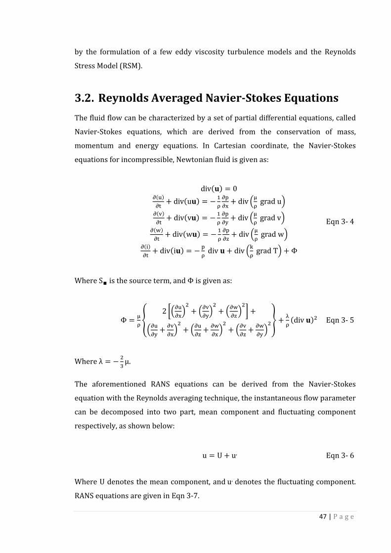
47 | P a g e
by the formulation of a few eddy viscosity turbulence models and the Reynolds
Stress Model (RSM).
3.2. Reynolds Averaged Navier-Stokes Equations
The fluid flow can be characterized by a set of partial differential equations, called
Navier-Stokes equations, which are derived from the conservation of mass,
momentum and energy equations. In Cartesian coordinate, the Navier-Stokes
equations for incompressible, Newtonian fluid is given as:
div��� = 0��3��� + div�u�� = − "U ���J + div Y�U gradu\������ + div�v�� = − "U ���R + div Y�U gradv\��s��� + div�w�� = − "U ���{ + div Y�U gradw\������ + div�i�� = − �U div� + div Y�U gradT\ + Φ Eqn 3- 4
Where S∎ is the source term, and Φ is given as:
Φ = �U � 2 �Y�3�J\� + Y���R\� + Y�s�{ \�� +Y�3�R + ���J\� + Y�3�{ + �s�J \� + Y���{ + �s�R \� + ¡U �div��� Eqn 3- 5
Where λ = − �� μ.
The aforementioned RANS equations can be derived from the Navier-Stokes
equation with the Reynolds averaging technique, the instantaneous flow parameter
can be decomposed into two part, mean component and fluctuating component
respectively, as shown below:
u = U + u, Eqn 3- 6
Where U denotes the mean component, and u, denotes the fluctuating component.
RANS equations are given in Eqn 3-7.
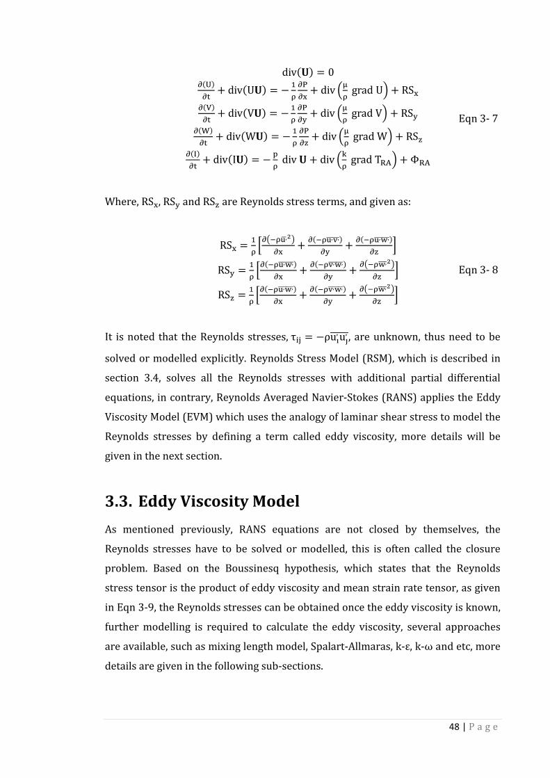
48 | P a g e
div�¢� = 0��H��� + div�U¢� = − "U �;�J + div Y�U gradU\ + RSJ��F��� + div�V¢� = − "U �;�R + div Y�U gradV\ + RSR��£��� + div�W¢� = − "U �;�{ + div Y�U gradW\ + RS{��¤��� + div�I¢� = − �U div¢ + div Y�U gradT¦§\ + Φ¦§
Eqn 3- 7
Where, RSJ, RSR and RS{ are Reynolds stress terms, and given as:
RSJ = "U ¨�5#U3,© '8�J + ��#U3,�,ªªªªª��R + ��#U3,s,ªªªªªª��{ «RSR = "U ¨��#U3,s,ªªªªªª��J + ��#U�,s,ªªªªªª��R + �5#Us,ªªª'8�{ «RS{ = "U ¨��#U3,s,ªªªªªª��J + ��#U�,s,ªªªªªª��R + �5#Us,ªªª'8�{ «
Eqn 3- 8
It is noted that the Reynolds stresses, τ�¬ = −ρu, u®,ªªªªª, are unknown, thus need to be
solved or modelled explicitly. Reynolds Stress Model (RSM), which is described in
section 3.4, solves all the Reynolds stresses with additional partial differential
equations, in contrary, Reynolds Averaged Navier-Stokes (RANS) applies the Eddy
Viscosity Model (EVM) which uses the analogy of laminar shear stress to model the
Reynolds stresses by defining a term called eddy viscosity, more details will be
given in the next section.
3.3. Eddy Viscosity Model
As mentioned previously, RANS equations are not closed by themselves, the
Reynolds stresses have to be solved or modelled, this is often called the closure
problem. Based on the Boussinesq hypothesis, which states that the Reynolds
stress tensor is the product of eddy viscosity and mean strain rate tensor, as given
in Eqn 3-9, the Reynolds stresses can be obtained once the eddy viscosity is known,
further modelling is required to calculate the eddy viscosity, several approaches
are available, such as mixing length model, Spalart-Allmaras, k-ε, k-ω and etc, more
details are given in the following sub-sections.
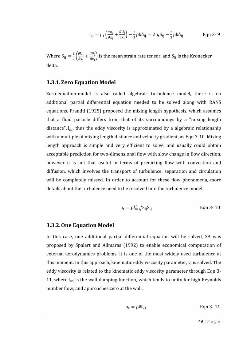
49 | P a g e
τ�¬ = μ� $�H°�J± + �H±�J° ) − �� ρkδ�¬ = 2μ�S�¬ − �� ρkδ�¬ Eqn 3- 9
Where S�¬ = "� $�H°�J± + �H±�J° ) is the mean strain rate tensor, and δ�¬ is the Kronecker
delta.
3.3.1. Zero Equation Model
Zero-equation-model is also called algebraic turbulence model, there is no
additional partial differential equation needed to be solved along with RANS
equations. Prandtl (1925) proposed the mixing length hypothesis, which assumes
that a fluid particle differs from that of its surroundings by a "mixing length
distance", l�, thus the eddy viscosity is approximated by a algebraic relationship
with a multiple of mixing length distance and velocity gradient, as Eqn 3-10. Mixing
length approach is simple and very efficient to solve, and usually could obtain
acceptable prediction for two-dimensional flow with slow change in flow direction,
however it is not that useful in terms of predicting flow with convection and
diffusion, which involves the transport of turbulence, separation and circulation
will be completely missed. In order to account for these flow phenomena, more
details about the turbulence need to be resolved into the turbulence model.
μ� = ρ´µ� ¶S�¬S�¬ Eqn 3- 10
3.3.2. One Equation Model
In this case, one additional partial differential equation will be solved, SA was
proposed by Spalart and Allmaras (1992) to enable economical computation of
external aerodynamics problems, it is one of the most widely used turbulence at
this moment. In this approach, kinematic eddy viscosity parameter, ν�, is solved. The
eddy viscosity is related to the kinematic eddy viscosity parameter through Eqn 3-
11, where f�" is the wall-damping function, which tends to unity for high Reynolds
number flow, and approaches zero at the wall.
μ� = ρν�f�" Eqn 3- 11

50 | P a g e
The transport equation to be solved is given as Eqn 3-12.
��U����� + div�ρν�¢� = "¹º div ¨�μ + ρν��grad�ν�� + C��ρ ����J»����J»«
+C�"ρν�Ω½ − Cs"ρ Y ��¾R\� fs Eqn 3- 12
Where Ω½ = Ω + ¿��ÀÁ� f�� , Ω is the mean vorticity, and Ω = ¶2Ω�¬Ω�¬ with
Ω�¬ = "� $�H°�J± − �H±�J° ), which is the mean vorticity tensor, σ�, C��, C�", Cs" and κ are
model constants, and given as follows:
σ� = �� C�� = 0.622C�" = 0.1355Cs" = C�" + κ� "uIo'¹º κ = 0.4187 Eqn 3- 13
Spalart-Allmaras (SA) model is specially designed for aerospace applications, and
recently, it becomes popular in turbomachinery applications. One kinematic eddy
viscosity parameter differential equation is solved along with RANS equations, thus
the computational cost is slightly higher than the mixing length model. It is capable
of predicting boundary layer flow very well even with adverse pressure gradient,
and it works well in the wall bounded flow with mild flow separation. It is
originally formulated as a low Reynolds turbulence model as stated by Spalart and
Allmaras, so the first grid point should be placed close to the wall, with small y+
value, in theory, it is not that suitable for flow with complex geometries due to the
difficulty in defining a proper length scale, moreover, it lacks sensitivity to
transport process in rapidly changing flows.
3.3.3. Two Equation Model
For two equation models, two additional differential equations are solved, common
two equation models are k-ε model, k-ω model and corresponding variants. Two
equation model is generally most accurate than zero and one equation models,
more information about the turbulence is taken into account, while they are more
computational expensive.

51 | P a g e
k-ε Model
k-ε model is the most widely used turbulence model in engineering application, it
can produce reasonably good results for free shear layer flows with small pressure
gradients, and wall bounded flow with zero or mild pressure gradients, however, it
has poor performance in the case of large adverse pressure gradients. The
predictions of the model are insensitive to the free stream turbulence parameters.
The standard k-ε model proposed by Launder and Spalding (1974) has two model
equation, for k and ε respectively. The formulation is given below:
��U���� + div�ρk¢� = div Y�&¹» gradk\ + 2μ�S�¬ ∙ S�¬ − ρε Eqn 3- 14
��UÈ��� + div�ρε¢� = div Y�&¹É gradε\ + C"È È� 2μ�S�¬ ∙ S�¬ − C�Èρ È'� Eqn 3- 15
and the eddy viscosity is modelled as:
μ� = ρC� �'È Eqn 3- 16
Where σ�, σÈ, C"È, C�È and C� are model constants and needed to be estimated from
experimental data. The general values are given as:
σ� = 1.00σÈ = 1.30C"È = 1.44C�È = 1.92C� = 0.09 Eqn 3- 17
k-ω Model
k-ω model (Wilcox, 1988) was developed in parallel with the k-ε model, it uses
specific dissipation rate ω as the second variable, the eddy viscosity can be
expressed as Eqn 3-18. k-ω model has superior performance in terms of numerical
stability in the viscous sublayer of wall bounded flow, this model does not require
explicit wall damping function, it gives good agreement with experimental results
for mild adverse pressure gradient flows. However, it is very sensitive to the free
stream turbulence parameters, thus is unsuitable for certain complex applications.
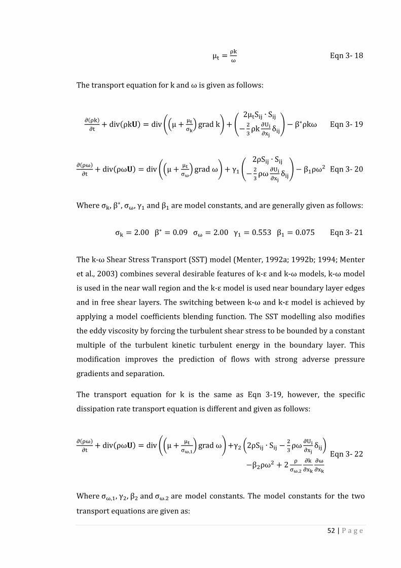
52 | P a g e
μ� = U�Ê Eqn 3- 18
The transport equation for k and ω is given as follows:
��U���� + div�ρk¢� = div ËYμ + �&¹»\ gradkÌ + Í 2μ�S�¬ ∙ S�¬− �� ρk �H°�J± δ�¬Î − β∗ρkω Eqn 3- 19
��UÊ��� + div�ρω¢� = div ËYμ + �&¹Ï\ gradωÌ + γ" Í 2ρS�¬ ∙ S�¬− �� ρω �H°�J± δ�¬Î − β"ρω� Eqn 3- 20
Where σ�, β∗, σÊ, γ" and β" are model constants, and are generally given as follows:
σ� = 2.00β∗ = 0.09σÊ = 2.00γ" = 0.553β" = 0.075 Eqn 3- 21
The k-ω Shear Stress Transport (SST) model (Menter, 1992a; 1992b; 1994; Menter
et al., 2003) combines several desirable features of k-ε and k-ω models, k-ω model
is used in the near wall region and the k-ε model is used near boundary layer edges
and in free shear layers. The switching between k-ω and k-ε model is achieved by
applying a model coefficients blending function. The SST modelling also modifies
the eddy viscosity by forcing the turbulent shear stress to be bounded by a constant
multiple of the turbulent kinetic turbulent energy in the boundary layer. This
modification improves the prediction of flows with strong adverse pressure
gradients and separation.
The transport equation for k is the same as Eqn 3-19, however, the specific
dissipation rate transport equation is different and given as follows:
��UÊ��� + div�ρω¢� = div Ë$μ + �&¹Ï,() gradωÌ +γ� $2ρS�¬ ∙ S�¬ − �� ρω �H°�J± δ�¬)−β�ρω� + 2 U¹Ï,' ���J»
�Ê�J» Eqn 3- 22
Where σÊ,", γ�, β� and σÊ.� are model constants. The model constants for the two
transport equations are given as:
53 | P a g e
σ� = 1.00β∗ = 0.09σÊ," = 2.00γ� = 0.44β� = 0.083σÊ,� = 1.17 Eqn 3- 23
Menter (1994) proposed a better expression for eddy viscosity with limiters, as
given below:
μ� = U�(���J��(Ê;SÑ'� Eqn 3- 24
Where a" is a model constant, and a" = 0.31, S is the mean strain rate, and S = ¶2S�¬S�¬. F� is a blending function.
3.4. Reynolds Stress Model
Second moment closure is also called Reynolds Stress Model (RSM), all the
Reynolds stresses are solved by the corresponding partial differential equations.
One-equation and two-equation turbulence models are all based on the
Boussinesq’s hypothesis. The Reynolds stresses cannot be correctly predicted in
the case of highly swirling anisotropic flow. Only RSM can predict the flow with
acceptable accuracy. In total, seven additional partial differential equations
(including ε partial differential equation) are solved along with the RANS equations.
The computational cost is much higher compared to other low order closures.
Linear and nonlinear pressure strain relations are available and works with wall
function. Early simulations on a selection of flows with RSM are reported in
Launder et al. (1975), the RSM transport equation can be written as:
v¦°±v� = �¦°±�� + C�¬ = P�¬ + D�¬ − ε�¬ + Π�¬ + Ω�¬ Eqn 3- 25
Where R�¬ = −τ�¬ ρ = u, u®,ªªªªª⁄ , C�¬ is the convection term, and the terms on the RHS
denotes production, diffusion, dissipation, pressure strain and rotation,
respectively. The convection, production and rotation terms can be derived and
expressed in their exact form, given as follows:
54 | P a g e
C�¬ = �YUH»3Ô, 3Õ,ªªªªªª\�J» = div5ρu, u®,ªªªªª¢8 Eqn 3- 26
P�¬ = − YR�� �H±�JW + R¬� �H°�JW\ Eqn 3- 27
Ω�¬ = −2ω�5u®, u�,ªªªªªªe��� + u, u�,ªªªªªªe¬��8 Eqn 3- 28
Where ω� is the rotation vector, and e�¬� is given as:
Öe�¬� = 1 ifi ≠ j ≠ kandcyclice�¬� = −1 ifi ≠ j ≠ kandanti − cyclice�¬� = 0 ifi = jorj = kori = k Û Eqn 3- 29
While the diffusion, dissipation and pressure strain terms are needed to be
modelled. Launder et al. (1975) and Rodi (1980) reported the details for the most
general models. Here, these terms are simply given as follows:
D�¬ = div Y ν&σ» gradR�¬\ Eqn 3- 30
ε�¬ = �� εδ�¬ Eqn 3- 31
Π�¬ = −C" ε� YR�¬ − �� kδ�¬\ − C� YP�¬ − �� Pδ�¬\ Eqn 3- 32
Where the kinematic eddy viscosity is calculated with:
ν� = �&U = C� �'È Eqn 3- 33
And C�, σ�, C" and C� are model constants, as given as:
C� = 0.09σ� = 1.0C" = 1.8C� = 0.6 Eqn 3- 34
55 | P a g e
The turbulent kinetic energy k is involved in Eqn 3-32, and can be calculated by
summation of diagonal Reynolds stresses.
Finally, the last transport equation for dissipation rate is given as:
vÈv� = div Y�&¹É gradε\ + C"È È� 2ν�S�¬ ∙ S�¬ − C�È È'� Eqn 3- 35
Where C"È and C�È are model constants, and given as:
C"ε = 1.44C�ε = 1.92 Eqn 3- 36
3.5. Summary
In this chapter, a brief introduction to the turbulence modelling was given, with
discussions on the capability of different turbulence models. Zero-equation model
is too simple to include flow details, such that it is not suitable for applications
involving transport of turbulence. SA model is a relatively new one-equation model,
it can be applied to flow with mild separation, however, it is not able to deal with
complex geometries due to the difficult in defining a length scale. Two-equation
model is more computational expensive, more details about the turbulence can be
taken into account, k-ε and k-ω models are among the most popular turbulence
models, the variant k-ω SST model incorporates k-ω and k-ε models, k-ω model is
used in the near wall region, and k-ε model is applied to regions far from the wall,
the prediction in large adverse pressure gradient is improved with k-ω SST model.
Zero-equation, one-equation and two-equation models are all based on the
Boussinesq hypothesis, which states that the Reynolds stresses can be expressed
with mean strain rates, while RSM is a second moment closure model, the Reynolds
stresses are solved explicitly with 6 transport equations. Highly anisotropic flow
with strong curvature and rotation can be predicted with very good accuracy.
However, the computational cost of RSM model is extremely high, thus it is not
always appropriate for certain applications. The most appropriate turbulence
model should be selected according the specific application.

56 | P a g e
Chapter 4 Methods of Investigation
Methods of Investigation
4.1. Introduction
This chapter presents the methods utilized in the investigation. First of all, the
assumptions made for this work are given, followed by the introduction to the
turbomachinery modelling methods, and then the grid generation process is
described, it is critical to have a good quality mesh to obtain acceptable prediction
results. After that, the general numerical conditions are described, including the
turbulence parameter estimation, boundary condition and interface selection, at
the end, the loss localization method is also discussed, and it will employed in the
following chapters to identify the regions of high loss generation.
4.2. Assumptions
General assumptions are usually essential before starting an investigation, where
simplification is generally required.
1. The centrifugal compressor flow field is assumed to be turbulent, in fact, the
flow should be transitional, with regions of laminar and turbulent flows.
However, it is generally difficult to predict the transitional flow reliably even
with the in-house LES. Commercial solver will be employed in this work,
considering the available computational resource and time, only simulation
with RANS approach is feasible, full annulus LES would be extremely time-
consuming and costly, or even not possible currently.

57 | P a g e
2. The inflow condition is assumed to be uniform without lose of generality.
3. No heat transfer is assumed to occur between the centrifugal compressor and
the environment, the wall is assumed to smooth and adiabatic.
4.3. Turbomachinery Modelling Techniques
The simulation of centrifugal compressor would include the rotating impeller and
stationary diffuser at the same time. In Star CCM+, two different approaches are
available, Multiple Reference Frame (MRF) and sliding mesh. MRF is useful for
steady simulation, while in order to capture the unsteadiness, a unsteady
simulation with sliding mesh is essential.
Another problem usually involved in turbomachinery modelling is the impeller-
diffuser pitch mismatch, different methods were proposed in literature, such as
domain scaling, mixing-plane, phase-lag boundary and harmonic balance method,
compared to the ordinary full annulus method, the application of these methods
can reduce the computational cost dramatically, only one passage is used during
the simulation, domain scaling and mixing-plane methods are relatively easy to
implement, while phase-lag boundary and harmonic balance method are very
difficult to program. Domain scaling method would scale either the impeller or the
diffuser or even both to obtain equivalent pitch angles, and the solidity should be
kept constant. One of the representative works is that of Rai and Madavan (1988).
Domain scaling method can be applied to both steady and unsteady simulations,
however, the scaling would inevitably cause certain level of inaccuracies. Mixing-
plane method works to take the circumferential average of the flow parameters,
and then passes the information to the next stage according to the interface area. It
is only suitable for steady simulation due to the mixing out of unsteadiness at the
interface. Phase-lag boundary was first proposed by Erdos and Alzner (1977), it is
based on the basic assumption that relative position of impeller and diffuser
determines the flow field inside the passage, in other words, the same relative
position would give rise to the same flow field. The adjacent passages are
approximated with a cyclic procedure, which asymptotically achieves the correct
phase between all passage. Harmonic balance method utilizes the Fourier series to
transform the unsteady time-periodic problem into steady state problem. It is only

58 | P a g e
applicable to flows with a regularly repeating flow pattern, Hall, Thomas and Clark
(2002) present a detailed description of harmonic balance method.
In star CCM+, mixing-plane and harmonic balance method are available, however,
to the author's knowledge, harmonic balance method is not fully developed in Star
CCM+ Version 8.04, and the parallelization is not fully implemented. So in this work,
steady simulation is conducted with mixing-plane interface and MRF, only one
passage is simulated. And unsteadiness is predicted through full annulus unsteady
simulation with sliding mesh.
4.4. Grid Generation
To obtain acceptable computational result, a good quality mesh is as important as
the solver. Low quality mesh will generally cause convergence problem, while
improperly clustered mesh would also produce unacceptable result. In principle,
fine mesh should be clustered in the high gradient regions, relatively coarse mesh
can be applied in far field regions or even be used artificially to damped out
vortices, which otherwise may cause reverse flow at outlet. In this thesis, two types
of grids are applied, multi-block structured mesh and polyhedral unstructured
mesh respectively.
4.4.1. Block-Structured Mesh
It is well known that structured mesh has many advantages over others, especially,
in turbomachinery applications. The cell can be aligned much better with the flow
direction, thus reduce the numerical diffusion and aiding convergence. Therefore,
block-structured mesh is used for the current work. The impeller blade is very
similar to the airfoil, except for the blunt trailing edge, so C-mesh is applied to
resolve the near wall boundary layer around the blade. H-mesh is applied in the
upstream, downstream and inside the passage. In this unshrouded impeller
simulation, the very small tip clearance has to be considered, CH-mesh is employed
with several layers of cells to resolve the flow inside the tip clearance. A schematic
is given in Figure 4- 1, the blocking strategy is very clearly demonstrated. During
the mesh generation process, caution has to be taken to ensure that the first layer

of mesh is located with
generated inside the boundary layer to resolve the near wall flow properly.
Globally, the cell aspect ratio should be less than 10, except for the near wall cells,
to resolve the boundary layer, the asp
growing ratio has to be less than 1.2 to achieve more stable and accurate result,
although 1.3 is a acceptable value for certain cases. Similarly, the block structured
mesh for the diffuser can be created with the
the only difference is that there is no tip clearance, and the diffuser blade has
curved leading and trailing
resolve the near wall boundary layer.
Figure 4
Figure 4- 2: Curved leading and trailing edge
of mesh is located with appropriate y+, and several layers of mesh has to be
generated inside the boundary layer to resolve the near wall flow properly.
Globally, the cell aspect ratio should be less than 10, except for the near wall cells,
to resolve the boundary layer, the aspect ratio will be very large, and the cell
growing ratio has to be less than 1.2 to achieve more stable and accurate result,
although 1.3 is a acceptable value for certain cases. Similarly, the block structured
mesh for the diffuser can be created with the blocking strategy shown
the only difference is that there is no tip clearance, and the diffuser blade has
curved leading and trailing edge, in the case, the O-mesh has to be applied to
resolve the near wall boundary layer.
Figure 4- 1: Blunt trailing edge impeller blocking strategy
: Curved leading and trailing edge diffuser blocking strategy
59 | P a g e
, and several layers of mesh has to be
generated inside the boundary layer to resolve the near wall flow properly.
Globally, the cell aspect ratio should be less than 10, except for the near wall cells,
ect ratio will be very large, and the cell
growing ratio has to be less than 1.2 to achieve more stable and accurate result,
although 1.3 is a acceptable value for certain cases. Similarly, the block structured
ing strategy shown in Figure 4- 2,
the only difference is that there is no tip clearance, and the diffuser blade has
mesh has to be applied to
: Blunt trailing edge impeller blocking strategy.
diffuser blocking strategy.
60 | P a g e
Ansys ICEM is a commercial grid generation package, which is available in the
School of MACE, the University of Manchester. The meshing procedure is that, first
of all, the fluid domain is split into a number of blocks, within which the mesh is
structured; then the edge parameter is set for each edge of the blocks, and thus the
block-structured mesh can be generated easily.
4.4.2. Polyhedral Unstructured Mesh
Polyhedral unstructured mesh is a relatively new concept, although general
commercial unstructured solver can deal with it appropriately, the mesh
generation itself is a difficult task. CD-adapco Star CCM+ has an embedded mesh
generator, which is capable of generating structured, tetrahedral and polyhedral
mesh automatically, with certain level of mesh optimization capability. According
to CD-Adapco (Peric, 2004), polyhedral mesh can be more promising compared to
tetrahedral mesh in terms of total number of cells and dealing with transport
property gradient, therefore, polyhedral mesh is adopted in this work for
comparison.
In Star CCM+, the polyhedral mesh can be generated together with surface
remesher and prism layer. The mesh generation procedure in Star CCM+ is that, the
surface mesh is generated at first, and is used as the basis for volume mesh
generation. Prism layer mesh is generally employed to resolve the near wall
boundary layer region, the prism layers will behave similarly to the structured
mesh near the wall. Certain criteria have to be fulfilled to gain some certainty about
the generated mesh, according to CD-adapco, the following three criteria should
applied to polyhedral mesh, the volume change should be greater than 1E-3, the
cell quality should be greater than 1E-6, and the skewness angle should be less than
85 deg. In the near wall region, the criteria for structured should be equally applied
to the polyhedral prism layer.
4.5. Numerical Conditions
Numerical simulation is also called numerical experiment, very similar to the
physical experiment, the numerical conditions have to be set up properly, such as

61 | P a g e
the turbulence parameters, boundary conditions, wall treatments and convergence
criteria.
4.5.1. Turbulence Parameters Estimation
In order to obtain acceptable computational result, it is critical to have a good
estimation of the turbulence parameters at the boundary. The general procedure is
given as follows:
Turbulence Intensity Estimation
1. Calculating the hydraulic diameter
D� = �§; Eqn 4- 1
2. Calculating the hydraulic diameter based inlet Reynolds number
Rev = ρH°ÜÝm&vÞμ
Eqn 4- 2
Where U�ß1à� is the inlet average velocity.
3. Estimation of the turbulence intensity
I ≈ 0.16�Rev�#" á⁄ Eqn 4- 3
Turbulence Length Scale Estimation
´ = 0.07D� Eqn 4- 4
Then the turbulence parameters for different turbulence models can be estimated
as follows:
62 | P a g e
Turbulent Kinetic Energy
k = �� �U�ß1à�I�� Eqn 4- 5
Turbulent Dissipation Rate
ε = Cμ� �⁄ �0 '⁄â Eqn 4- 6
Where C� is a model constant and equals to 0.09.
Specific Dissipation Rate
ω = �( '⁄Iμ( ã⁄ â Eqn 4- 7
Eddy Viscosity Parameter
ν� = z�� U�ß1à�I´ Eqn 4- 8
4.5.2. Boundary Conditions
For a typical turbomachinery simulation, stagnation inlet and mass flow inlet
boundary conditions could be applied, in this case, the mass flow inlet was selected
in consideration of the available experimental conditions. The inflow direction was
set to normal to the inlet surface, additionally, uniform velocity was used with the
estimated turbulence parameters. In order to save the computational time, only a
single passage was simulated for steady simulation, thus requires the use of
periodic boundary condition at each side of the passage. In the case of full annulus
unsteady simulation, there is no need for periodic boundary conditions. Static
pressure is specified at the outlet, as well as the temperature.
63 | P a g e
4.5.3. Wall treatments
Wall treatment is an essential part of the simulation, and it can help predict the
near wall flow field, which is usually very important due to the highly viscous and
dissipative nature. In Star CCM+, three different wall treatments are available, high-yu wall treatment, low-yu wall treatment and all-yu wall treatment. High-yu wall
treatment employs the wall function to account for the boundary layer, the near-
wall cell should lie within the logarithmic region of the boundary layer. Low-yu
wall treatment is suitable for low-Reynolds number turbulence model only, the
viscous sublayer is assumed to be resolved with near-wall cells. All-yu wall
treatment is recommended in Star CCM+ User Guide Version 8.04 (CD-adapco,
2013) and is a hybrid treatment, it behaves like high-yu wall treatment if the mesh
is coarse, and like low-yu wall treatment if the mesh is fine enough, it is also
capable of dealing with meshes of intermediate resolution. All-yu wall treatment is
available for SA, k-ε and k-ω models, thus it is used for all simulations in this work.
4.5.4. Convergence Criteria
Numerical simulation is actually a process of solving partial differential equations
with numerical method, which produces the approximated rather than exact
solution, thus convergence criteria are required to assess whether the
approximated solution has been close enough to the exact solution or not. In
practice, the exact solution is always unknown, as a result, the difference between
successive solutions is used as the convergence criterion, called residual. In CFD,
convergence criteria are applied to ensure that the flow field is converged enough,
thus produce meaningful flow field prediction. The continuity, momentum and
energy residuals are usually monitored, when turbulence models are involved, the
turbulence parameter residuals are also need to be taken into account. In this
specific application, additional convergence criteria are selected as the torque
produced by the rotating impeller and the airwatt. The residuals are generally
required to be dropped below 1E-4 for convergence in this work, however, for
steady simulation at off design condition, the criteria are relaxed to 1E-3,
additionally, the torque and airwatt should flatten out for convergence.
64 | P a g e
4.6. Loss Localization Method
Although entropy generation has been introduced to quantify the loss occurred
inside the turbomachinery, the local loss is more difficult to obtain, while it is the
local loss that really affect the design. The knowledge on the position and
magnitude of local losses can help the designer to improve the performance
through local geometry modification, thus reduce the extent and magnitude of high
loss regions.
There are two mechanisms that could be responsible for local entropy generation,
e.g. shear strain and thermal gradient. Sciubba (1994) proposed to use these local
flow quantities to express the entropy generation and split the entropy generation
to two parts, viscous entropy generation and thermal entropy generation
respectively, as shown in Eqn 4-9, where μà and kà is the effective eddy viscosity
and effective thermal conductivity respectively, and the entropy generation rate is
calculated per unit volume, with unit W �m�K�⁄ . The entropy generations due to
viscous effect and thermal effect can be written more explicitly, as given in Eqn 4-
10 and Eqn 4-11 respectively, where they are expressed as strain rate and thermal
gradient in Cartesian coordinate system.
�-�� = s = sF + sE = μà äE + kà ∇'EE' Eqn 4- 9
sF = �mE �2 �Y�3�J\� + Y���R\� + Y�s�{ \�� + Y�3�{ + �s�J \�+ Y�3�R + ���J\� + Y���{ + �s�R \� Eqn 4- 10
sE = �mE' �Y�E�J\� + Y�E�R\� + Y�E�{\�� Eqn 4- 11
4.7. Summary
The methods of investigation related to numerical simulation were discussed in
this chapter. At the beginning, the turbomachinery modelling methods were
introduced. Single passage steady simulation and full annulus unsteady simulation

65 | P a g e
were employed to investigate the flow behaviour inside centrifugal compressor.
Then the numerical conditions on the simulation set-up were described, the
boundary conditions would be set to mass flow inlet (or velocity inlet for
incompressible flow) and static pressure outlet. As recommended by Star CCM+
User Guide Version 8.04 (CD-adapco, 2013), the all-yu wall treatment would be
employed throughout this work, the convergence criteria were also determined,
the residuals should all drop below 1E-3, the torque and airwatt should flatten out
for convergence. At the end, the loss localization method was also discussed, and
could be used to identify the regions of high local loss generation.

66 | P a g e
Chapter 5 Validation of Star CCM+ Solver
Validation of Star CCM+ Solver
5.1. Introduction
Centrifugal compressors are generally of complex geometry, strong curvature,
effect of centrifugal force and Coriolis force complicate the flow field, as well as the
interactions between different flow features. The flow is viscous, highly unsteady,
swirling and transitional. Consequently, it is very difficult to obtain an acceptable
prediction.
Star CCM+ is a commercial CFD solver available in the market, and becomes very
popular recently, and it is selected as the solver for the current work. This chapter
intends to give a brief introduction to Star CCM+ at first, and then solver validation
is conducted to verify its capability in predicting the performance and flow field
inside centrifugal compressors with the available experimental data.
5.2. CD-adapco Star CCM+ Solver
A number of commercial CFD packages are available on the shelf, Ansys CFX, Ansys
Fluent, Numeca Fine, CD-adapco Star CCM+ and etc, they are generally of high cost
and very powerful, it is not feasible to buy anyone of them personally. The School of
MACE (the University of Manchester) has some of them installed on the
Computational Shared Facility (CSF), such as CFX, Fluent and Star CCM+. CSF is a
high performance computing cluster built for research groups in the university, it
has about 5,000 processors at this moment. Considering the limitation on license,
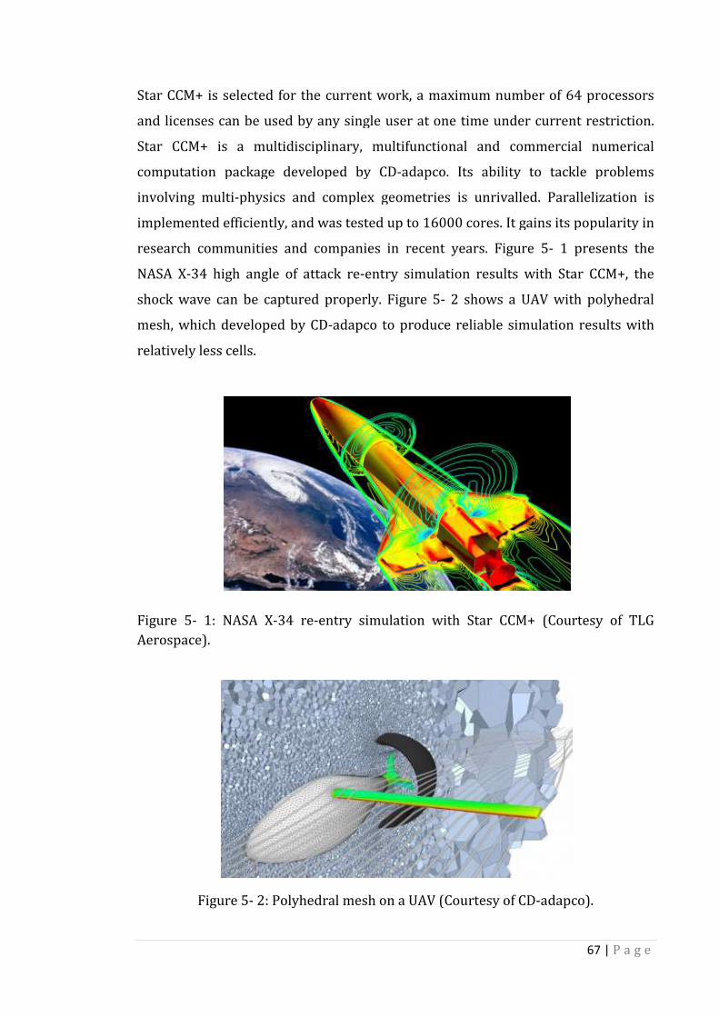
Star CCM+ is selected for t
and licenses can be used by any single user at one time under current restriction.
Star CCM+ is a multidisciplinary
computation package developed by CD
involving multi-physics and complex geometries is unrivalled. Parallelization is
implemented efficiently, and was tested up to 16000 cores.
research communities and companies in recent years.
NASA X-34 high angle of attack re
shock wave can be captured properly.
mesh, which developed by CD
relatively less cells.
Figure 5- 1: NASA X
Aerospace).
Figure 5- 2
Star CCM+ is selected for the current work, a maximum number of 64 processors
and licenses can be used by any single user at one time under current restriction.
multidisciplinary, multifunctional and commercial numerical
computation package developed by CD-adapco. Its ability to tackle problems
physics and complex geometries is unrivalled. Parallelization is
implemented efficiently, and was tested up to 16000 cores. It gains its popularity in
research communities and companies in recent years. Figure 5
34 high angle of attack re-entry simulation results with Star CCM+, the
an be captured properly. Figure 5- 2 shows a UAV with polyhedral
mesh, which developed by CD-adapco to produce reliable simulation results with
: NASA X-34 re-entry simulation with Star CCM+ (Courtesy of TLG
2: Polyhedral mesh on a UAV (Courtesy of CD
67 | P a g e
he current work, a maximum number of 64 processors
and licenses can be used by any single user at one time under current restriction.
, multifunctional and commercial numerical
s ability to tackle problems
physics and complex geometries is unrivalled. Parallelization is
It gains its popularity in
Figure 5- 1 presents the
entry simulation results with Star CCM+, the
shows a UAV with polyhedral
adapco to produce reliable simulation results with
simulation with Star CCM+ (Courtesy of TLG
: Polyhedral mesh on a UAV (Courtesy of CD-adapco).
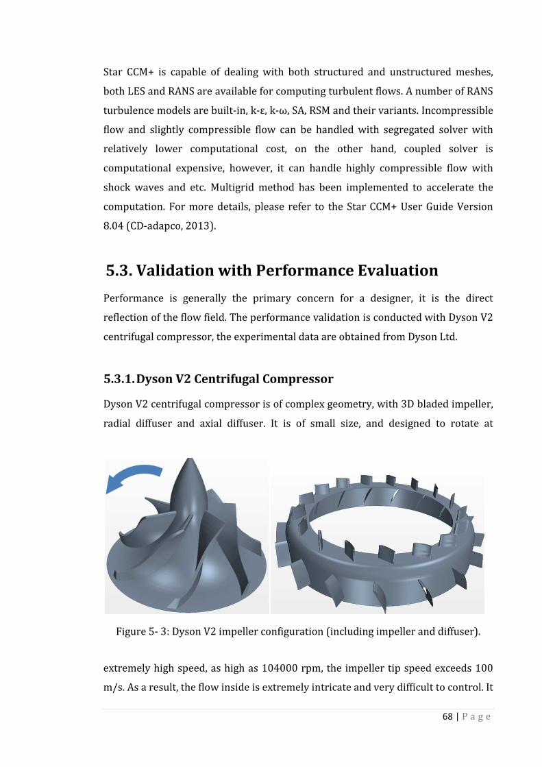
68 | P a g e
Star CCM+ is capable of dealing with both structured and unstructured meshes,
both LES and RANS are available for computing turbulent flows. A number of RANS
turbulence models are built-in, k-ε, k-ω, SA, RSM and their variants. Incompressible
flow and slightly compressible flow can be handled with segregated solver with
relatively lower computational cost, on the other hand, coupled solver is
computational expensive, however, it can handle highly compressible flow with
shock waves and etc. Multigrid method has been implemented to accelerate the
computation. For more details, please refer to the Star CCM+ User Guide Version
8.04 (CD-adapco, 2013).
5.3. Validation with Performance Evaluation
Performance is generally the primary concern for a designer, it is the direct
reflection of the flow field. The performance validation is conducted with Dyson V2
centrifugal compressor, the experimental data are obtained from Dyson Ltd.
5.3.1. Dyson V2 Centrifugal Compressor
Dyson V2 centrifugal compressor is of complex geometry, with 3D bladed impeller,
radial diffuser and axial diffuser. It is of small size, and designed to rotate at
Figure 5- 3: Dyson V2 impeller configuration (including impeller and diffuser).
extremely high speed, as high as 104000 rpm, the impeller tip speed exceeds 100
m/s. As a result, the flow inside is extremely intricate and very difficult to control. It

69 | P a g e
is located just downstream of the cyclone separator, for which the suction power is
provided to separate dust particle from the air. The discharge from the Dyson V2
centrifugal compressor is further used to cool the electric motor which supplies
shaft work to the impeller. Figure 5- 3 presents the key components of Dyson V2
centrifugal compressor. The impeller design operation condition is given in Table
5- 1 (according to Dyson Ltd.), as well as the detailed geometric parameters for
impeller and diffuser stages.
Operating Conditions
Rotational speed (design) 85907 rpm
Mass flow rate 0.015252 kg/s
Reynolds number (inlet) 54000
Impeller
Inlet inner diameter 0.76 mm
Inlet outer diameter 19.84 mm
Outlet diameter 33.10 mm
Blade leading edge span 6.10 mm
Blade trailing edge span 2.51 mm
Number of blades 7
Tip clearance height* 0.25-0.26 mm
Backsweep angle 47 deg
Diffuser
Inlet diameter 36.41 mm
Outlet inner diameter 45.87 mm
Outlet outer diameter 51.80 mm
Number of diffusers 2
Number of blades 17
Radial diffuser blade span 2.76 mm
Axial diffuser blade span* 2.49-2.98 mm
Table 5- 1: Dyson V2 centrifugal compressor geometry parameters.
A number of simulation cases have been run at different operation conditions,
which are constant power operation conditions according to Dyson Ltd., details are
given in Table 5- 2. It is noted that Case 1 corresponds to the impeller design
operation condition as presented in Table 5- 1.

70 | P a g e
Rotational Speed (rpm) Mass Flow Rate (kg/s)
Case 1 85907 1.5254E-2
Case 2 89146 1.3087E-2
Case 3 92818 1.0655E-2
Case 4 95084 9.3804E-3
Case 5 97945 8.0837E-3
Case 6 101729 6.8508E-3
Table 5- 2: Dyson V2 centrifugal compressor performance evaluation cases.
5.3.2. Numerical Conditions
Steady simulation is conducted for performance evaluation and flow field analysis,
instead of simulating the full annulus configuration, a single passage is simulated
for the sake of time and computational cost. Moving Reference Frame (MRF) is
employed to account for the relative motion between the impeller and diffuser, k-ω
SST turbulence model is applied to deal with the turbulence involved, SA and
realisable k-ε turbulence models are also used, the results are compared with that
of k-ω SST, more details are given in Appendix A. Figure 5- 4 shows the
configuration for the steady simulation, two passages are presented for clarity. In
order to enable the single passage steady simulation, rotational periodicity is
specified to reduce the full annulus to a single passage, and mixing plane interface
is employed to solve the impeller-diffuser blade pitch mismatch problem, thus pass
the flow information properly from rotating impeller to downstream stationary
diffuser. The block-structured mesh is generated with the aforementioned mesh
generation method. Figure 5- 5 and Figure 5- 6 show the block-structured mesh for
impeller and diffuser respectively. The mesh at one streamwise location for
impeller is presented in Figure 5- 7, the tip clearance is well resolved with several
layers of mesh. The inlet boundary is set to mass flow inlet, and static pressure is
specified for the outlet, other boundaries are set to no-slip, adiabatic wall.

71 | P a g e
Figure 5- 4: Dyson V2 steady simulation configuration.
Figure 5- 5: Dyson V2 impeller block-structured mesh.
Impeller Blade
Near Wall Fine Mesh

Figure 5
Figure 5- 7: Streamwise cross section mesh for Dyson V2 impeller
5.3.3. Results
The overall performance curves are plotted in
regard to airwatt, efficiency and pressure ratio respectively,
are compared with the experimental results when av
8, despite the airwatt is over
Figure 5- 6: Dyson V2 vaned diffuser block-structured mesh
: Streamwise cross section mesh for Dyson V2 impeller
The overall performance curves are plotted in Figure 5- 8 to
airwatt, efficiency and pressure ratio respectively,
are compared with the experimental results when available. Referring to
, despite the airwatt is over-predicted by the numerical simulation, the computed
72 | P a g e
structured mesh.
: Streamwise cross section mesh for Dyson V2 impeller.
to Figure 5- 10, with
airwatt, efficiency and pressure ratio respectively, the numerical results
ailable. Referring to Figure 5-
numerical simulation, the computed
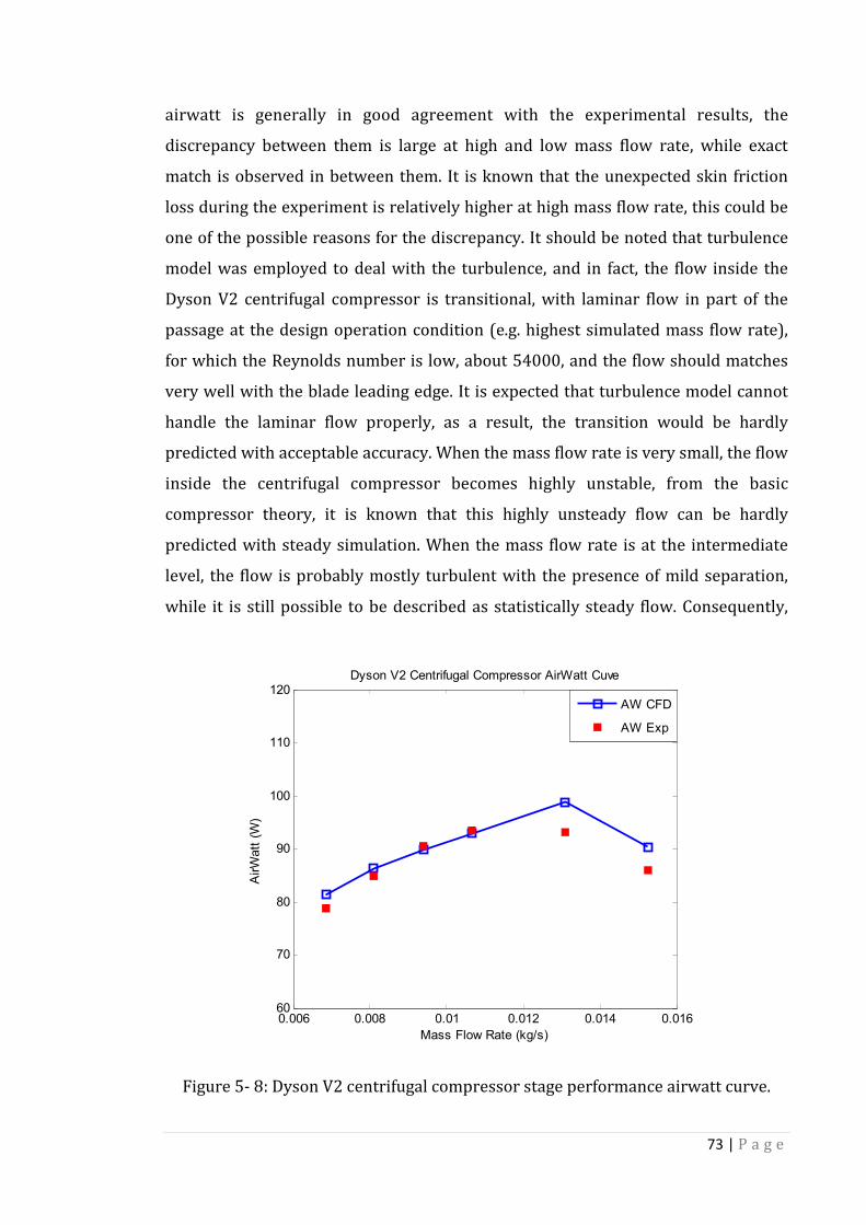
73 | P a g e
airwatt is generally in good agreement with the experimental results, the
discrepancy between them is large at high and low mass flow rate, while exact
match is observed in between them. It is known that the unexpected skin friction
loss during the experiment is relatively higher at high mass flow rate, this could be
one of the possible reasons for the discrepancy. It should be noted that turbulence
model was employed to deal with the turbulence, and in fact, the flow inside the
Dyson V2 centrifugal compressor is transitional, with laminar flow in part of the
passage at the design operation condition (e.g. highest simulated mass flow rate),
for which the Reynolds number is low, about 54000, and the flow should matches
very well with the blade leading edge. It is expected that turbulence model cannot
handle the laminar flow properly, as a result, the transition would be hardly
predicted with acceptable accuracy. When the mass flow rate is very small, the flow
inside the centrifugal compressor becomes highly unstable, from the basic
compressor theory, it is known that this highly unsteady flow can be hardly
predicted with steady simulation. When the mass flow rate is at the intermediate
level, the flow is probably mostly turbulent with the presence of mild separation,
while it is still possible to be described as statistically steady flow. Consequently,
Figure 5- 8: Dyson V2 centrifugal compressor stage performance airwatt curve.
0.006 0.008 0.01 0.012 0.014 0.01660
70
80
90
100
110
120
Mass Flow Rate (kg/s)
AirW
att
(W
)
Dyson V2 Centrifugal Compressor AirWatt Cuve
AW CFD
AW Exp
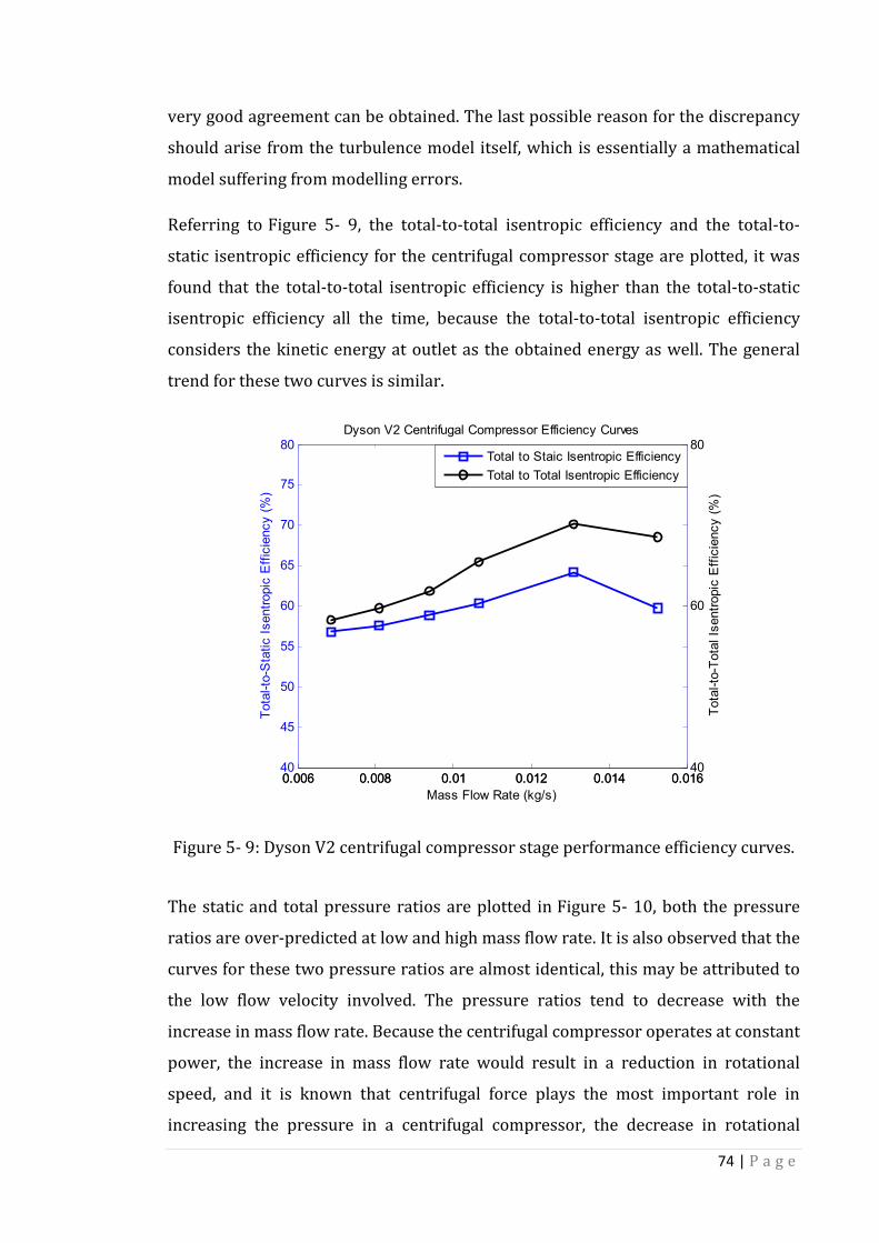
74 | P a g e
very good agreement can be obtained. The last possible reason for the discrepancy
should arise from the turbulence model itself, which is essentially a mathematical
model suffering from modelling errors.
Referring to Figure 5- 9, the total-to-total isentropic efficiency and the total-to-
static isentropic efficiency for the centrifugal compressor stage are plotted, it was
found that the total-to-total isentropic efficiency is higher than the total-to-static
isentropic efficiency all the time, because the total-to-total isentropic efficiency
considers the kinetic energy at outlet as the obtained energy as well. The general
trend for these two curves is similar.
Figure 5- 9: Dyson V2 centrifugal compressor stage performance efficiency curves.
The static and total pressure ratios are plotted in Figure 5- 10, both the pressure
ratios are over-predicted at low and high mass flow rate. It is also observed that the
curves for these two pressure ratios are almost identical, this may be attributed to
the low flow velocity involved. The pressure ratios tend to decrease with the
increase in mass flow rate. Because the centrifugal compressor operates at constant
power, the increase in mass flow rate would result in a reduction in rotational
speed, and it is known that centrifugal force plays the most important role in
increasing the pressure in a centrifugal compressor, the decrease in rotational
0.006 0.008 0.01 0.012 0.014 0.01640
45
50
55
60
65
70
75
80
Mass Flow Rate (kg/s)
Tota
l-to
-Sta
tic I
sentr
opic
Eff
icie
ncy (
%)
Dyson V2 Centrifugal Compressor Efficiency Curves
0.006 0.008 0.01 0.012 0.014 0.01640
60
80
Tota
l-to
-Tota
l Is
entr
opic
Eff
icie
ncy (
%)
Total to Staic Isentropic Efficiency
Total to Total Isentropic Efficiency
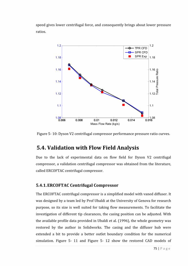
75 | P a g e
speed gives lower centrifugal force, and consequently brings about lower pressure
ratios.
Figure 5- 10: Dyson V2 centrifugal compressor performance pressure ratio curves.
5.4. Validation with Flow Field Analysis
Due to the lack of experimental data on flow field for Dyson V2 centrifugal
compressor, a validation centrifugal compressor was obtained from the literature,
called ERCOFTAC centrifugal compressor.
5.4.1. ERCOFTAC Centrifugal Compressor
The ERCOFTAC centrifugal compressor is a simplified model with vaned diffuser. It
was designed by a team led by Prof Ubaldi at the University of Genova for research
purpose, so its size is well suited for taking flow measurements. To facilitate the
investigation of different tip clearances, the casing position can be adjusted. With
the available profile data provided in Ubaldi et al. (1996), the whole geometry was
restored by the author in Solidworks. The casing and the diffuser hub were
extended a bit to provide a better outlet boundary condition for the numerical
simulation. Figure 5- 11 and Figure 5- 12 show the restored CAD models of
0.006 0.008 0.01 0.012 0.014 0.0161.08
1.1
1.12
1.14
1.16
1.18
1.2
Mass Flow Rate (kg/s)
0.006 0.008 0.01 0.012 0.014 0.0161.08
1.1
1.12
1.14
1.16
1.18
1.2
Tota
l P
ressure
Ratio
TPR CFD
SPR CFD
SPR Exp

76 | P a g e
impeller hub & blades and diffuser hub & blades respectively. The basic geometric
data and operating conditions are given in Table 5- 3. According to Ubaldi et al., the
tip clearance was set to the minimum value of 0.4 mm during their experiment to
reduce the tip leakage flow effect. A constant-temperature hot-wire anemometer
with single sensor probes was used by Ubaldi et al. to measure the three
dimensional unsteady flow field at the impeller outlet, and the static pressure
distribution on the impeller casing was measured with fast response pressure
transducers along the radial direction. Certain flow field measurements are
available and extracted with Matlab, such as the radial and tangential velocities at
the impeller outlet, the pressure coefficient on the casing. For more details, please
refer to Ubaldi et al. (1996).
Figure 5- 11: ERCOFTAC centrifugal pump 2D blade impeller.
Figure 5- 12: ERCOFTAC centrifugal pump 2D blade diffuser.
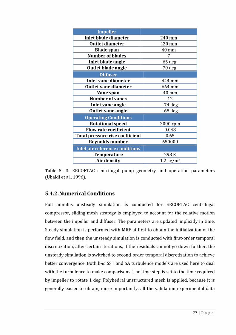
77 | P a g e
Impeller
Inlet blade diameter 240 mm
Outlet diameter 420 mm
Blade span 40 mm
Number of blades 7
Inlet blade angle -65 deg
Outlet blade angle -70 deg
Diffuser
Inlet vane diameter 444 mm
Outlet vane diameter 664 mm
Vane span 40 mm
Number of vanes 12
Inlet vane angle -74 deg
Outlet vane angle -68 deg
Operating Conditions
Rotational speed 2000 rpm
Flow rate coefficient 0.048
Total pressure rise coefficient 0.65
Reynolds number 650000
Inlet air reference conditions
Temperature 298 K
Air density 1.2 kg/m3
Table 5- 3: ERCOFTAC centrifugal pump geometry and operation parameters
(Ubaldi et al., 1996).
5.4.2. Numerical Conditions
Full annulus unsteady simulation is conducted for ERCOFTAC centrifugal
compressor, sliding mesh strategy is employed to account for the relative motion
between the impeller and diffuser. The parameters are updated implicitly in time.
Steady simulation is performed with MRF at first to obtain the initialization of the
flow field, and then the unsteady simulation is conducted with first-order temporal
discretization, after certain iterations, if the residuals cannot go down further, the
unsteady simulation is switched to second-order temporal discretization to achieve
better convergence. Both k-ω SST and SA turbulence models are used here to deal
with the turbulence to make comparisons. The time step is set to the time required
by impeller to rotate 1 deg. Polyhedral unstructured mesh is applied, because it is
generally easier to obtain, more importantly, all the validation experimental data

78 | P a g e
were collected by Ubaldi et al. (1996) at the narrow vaneless space between the
impeller and diffuser, the resolution of the flow structure is not of interest.
5.4.3. Results
The instantaneous results were measured at different instants with reference to
one specific time instant T and at specific radial and circumferential positions,
which was chosen by Ubaldi et al. (1996) during their experiment. A non-
dimensional time instant is defined as:
æ = çèé Eqn 5- 1
Where Ti is the rotor blade passing period, as defined as:
æê = �ëìíé Eqn 5- 2
Where ω is the rotor angular speed, and zi is the impeller blade number.
The instantaneous radial and tangential velocities were extracted from simulation
results at the impeller outlet (at 2d/Di=1.02, where d is the distance from the
centre, and Di is the impeller diameter) for non-dimensional time instant 0.126,
0.226, 0.326 and 0.426. For example, T=0.426 would mean that the blade has
moved a distance about half of the blade pitch.
The instantaneous non-dimensional radial velocities are plotted against non-
dimensional circumferential distance and shown in Figure 5- 13 to Figure 5- 16 for
different non-dimensional time instants, the corresponding experimental data are
included for comparison. The non-dimensional circumferential distance is the
circumferential distance normalized by the impeller blade pitch. The black tiangles
denote the impeller blade positions, and the black squares denote the diffuser
blade positions. It is observed that the computed instantaneous non-dimensioanl
radial velocities are generally consistent with the experimental results, however,
the peak values are under-estimated with numerical simulations, this could be

79 | P a g e
Figure 5- 13: Non-dimensioanl radial velocity at time instant T=0.126.
Figure 5- 14: Non-dimensional radial velocity at time instant T=0.226.
0 0.5 1 1.5 20
0.1
0.2
0.3
0.4
0.5
Nondimensional Circumferential Distance
Nondim
ensio
nal R
adia
l V
elo
city
Radial Velocity at Time Instant T=0.126
Exp
CFD SA
CFD k-w SST
0 0.5 1 1.5 20
0.1
0.2
0.3
0.4
0.5
Nondimensional Circumferential Distance
Nondim
ensio
nal R
adia
l V
elo
city
Radial Velocity at Time Instant T=0.226
Exp
CFD SA
CFD k-w SST

80 | P a g e
Figure 5- 15: Non-dimensional radial velocity at time isntant T=0.326.
Figure 5- 16: Non-dimensional radial velocity at time instant T=0.426.
0 0.5 1 1.5 20
0.1
0.2
0.3
0.4
0.5
Nondimensional Circumferential Distance
Nondim
ensio
nal R
adia
l V
elo
city
Radial Velocity at Time Instant T=0.326
Exp
CFD SA
CFD k-w SST
0 0.5 1 1.5 20
0.1
0.2
0.3
0.4
0.5
Nondimensional Circumferential Distance
Nondim
ensio
nal R
adia
l V
elo
city
Radial Velocity at Time Instant T=0.426
Exp
CFD SA
CFD k-w SST

81 | P a g e
caused by the presence of diffuser blades, which generate disturbances (back
propagation pressure) and cannot be modelled properly by both turbulence models.
Another possible reason could be that the employed polyhedral mesh is not fine
enough, the disturbances are subject to numerical diffusion, as a result, the
magnitude is attenuated. The computed results from both turbulence models are
extremely consistent, the flow details are almost eactly the same. It must be also
noted that ensemble averaging was used for the experimental data, however, the
computed results are instantaneous values due to the computational burden in
conducting long physical time simulation, so it should be reasonable to expect
certain degree of discrepancy. Well defined wake could also be observed just
downstream of the impeller blades. The velocity mimima is generally located at the
pressure side of the wake. And tiny troughs are observed to locate just upstream of
the diffuser blades due to the deceleration of the air stream caused by the presence
of diffuser blades, the "jet-wake structure" is clearly identified as well.
Figure 5- 17: Non-dimensional tangential velocity at time instant 0.126.
0 0.5 1 1.5 2-0.9
-0.8
-0.7
-0.6
-0.5
-0.4-0.4
Nondimensional Circumferential Distance
Nondim
ensio
nal T
angential V
elo
city
Tangential Velocity at Time Instant T=0.126
Exp
CFD SA
CFD k-w SST

82 | P a g e
Figure 5- 18: Non-dimensional tangential velocity at time instant 0.226.
Figure 5- 19: Non-dimensional tangential velocity at time instant 0.326.
0 0.5 1 1.5 2-0.9
-0.8
-0.7
-0.6
-0.5
-0.4-0.4
Nondimensional Circumferential Distance
Nondim
ensio
nal T
angential V
elo
city
Tangential Velocity at Time Instant T=0.226
Exp
CFD SA
CFD k-w SST
0 0.5 1 1.5 2-0.9
-0.8
-0.7
-0.6
-0.5
-0.4-0.4
Nondimensional Circumferential Distance
Nondim
ensio
nal T
angential V
elo
city
Tangential Velocity at Time Instant T=0.326
Exp
CFD SA
CFD k-w SST
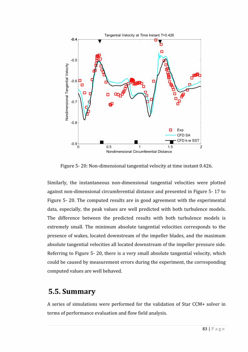
83 | P a g e
Figure 5- 20: Non-dimensional tangential velocity at time instant 0.426.
Similarly, the instantaneous non-dimensional tangential velocities were plotted
against non-dimensional circumferential distance and presented in Figure 5- 17 to
Figure 5- 20. The computed results are in good agreement with the experimental
data, especially, the peak values are well predicted with both turbulence models.
The difference between the predicted results with both turbulence models is
extremely small. The minimum absolute tangential velocities corresponds to the
presence of wakes, located downstream of the impeller blades, and the maximum
absolute tangential velocities all located downstream of the impeller pressure side.
Referring to Figure 5- 20, there is a very small absolute tangential velocity, which
could be caused by measurement errors during the experiment, the corresponding
computed values are well behaved.
5.5. Summary
A series of simulations were performed for the validation of Star CCM+ solver in
terms of performance evaluation and flow field analysis.
0 0.5 1 1.5 2-0.9
-0.8
-0.7
-0.6
-0.5
-0.4-0.4
Nondimensional Circumferential Distance
Nondim
ensio
nal T
angential V
elo
city
Tangential Velocity at Time Instant T=0.426
Exp
CFD SA
CFD k-w SST

84 | P a g e
The validation simulation on performance evaluation was conducted for Dyson V2
centrifugal compressor, with the experimental results provided by Dyson Ltd.
Single passage steady simulation with mixing-plane interface and MRF was
employed here. Performance curves were plotted, including airwatt, isentropic
efficiencies and pressure ratios. The computed results show good agreements with
the experimental data, although discrepancies were found due to possible
turbulence modelling error, physical modelling error and experimental
measurement uncertainties. The results with different turbulence models were
presented in Appendix A, k-ω SST turbulence model gives slightly better results
compared to SA and realizable k-ε turbulence models.
Due to the lack of flow field measurements on Dyson V2 centrifugal compressor, a
validation case was obtained from literature, called the ERCOFTAC centrifugal
compressor. Flow field measurements at the vaneless space between the impeller
and diffuser are available, the results from the full annulus unsteady simulation
were plotted against the experimental results, good agreements were found,
although the peak values of radial velocity were generally under-predicted, the
trend and flow patterns were similar. k-ω SST and SA turbulence models were
compared, exact match between their predicted results were almost obtained,
there is no conclusion on the superiority of either k-ω SST or SA turbulence models.
However, k-ω SST turbulence model is supposed to have better performance in
predicting flow with separation, and it is able to handle flow with complex
geometry.
In total, the validation cases on performance evaluation and flow field analysis
show that Star CCM+ is suitable for the current application, and can produce
acceptable results. k-ω SST turbulence model will be employed in following chapter
for further analysis.

85 | P a g e
Chapter 6 Flow Field Analysis
Flow Field Analysis
6.1. Introduction
In this chapter, the flow field analysis is conducted for Dyson V2 centrifugal
compressor at Case 1 through single passage steady simulation with k-ω SST
turbulence model, with emphasis on the impeller. Steady simulation is good for
presenting a general picture of the flow field and much easier to obtain in terms of
computational cost, thus it is generally useful during the design process. Different
flow features are illustrated and discussed with reference to the performance, so
are the primary losses. The predicted wall shear stress and skin friction lines on
impeller hub will be used to determine the riblets size in chapter 8. The simulation
set-up was given in section 5.1, and will not be described here again. The grid
independence study is conducted, three different grid resolutions are examined,
and the corresponding results are given in Appendix B.
6.2. Results
Some results are discussed with regard to different regions of the compressor, so
Dyson V2 centrifugal compressor has been split into four different regions, impeller,
radial diffuser, 90 deg bend and axial diffuser, respectively, as illustrated in Figure
6- 1, different streamwise stations are also shown, stations 1 to 4 are in the
impeller region, stations 5 and 6 are in the radial diffuser region, station 7 is in the
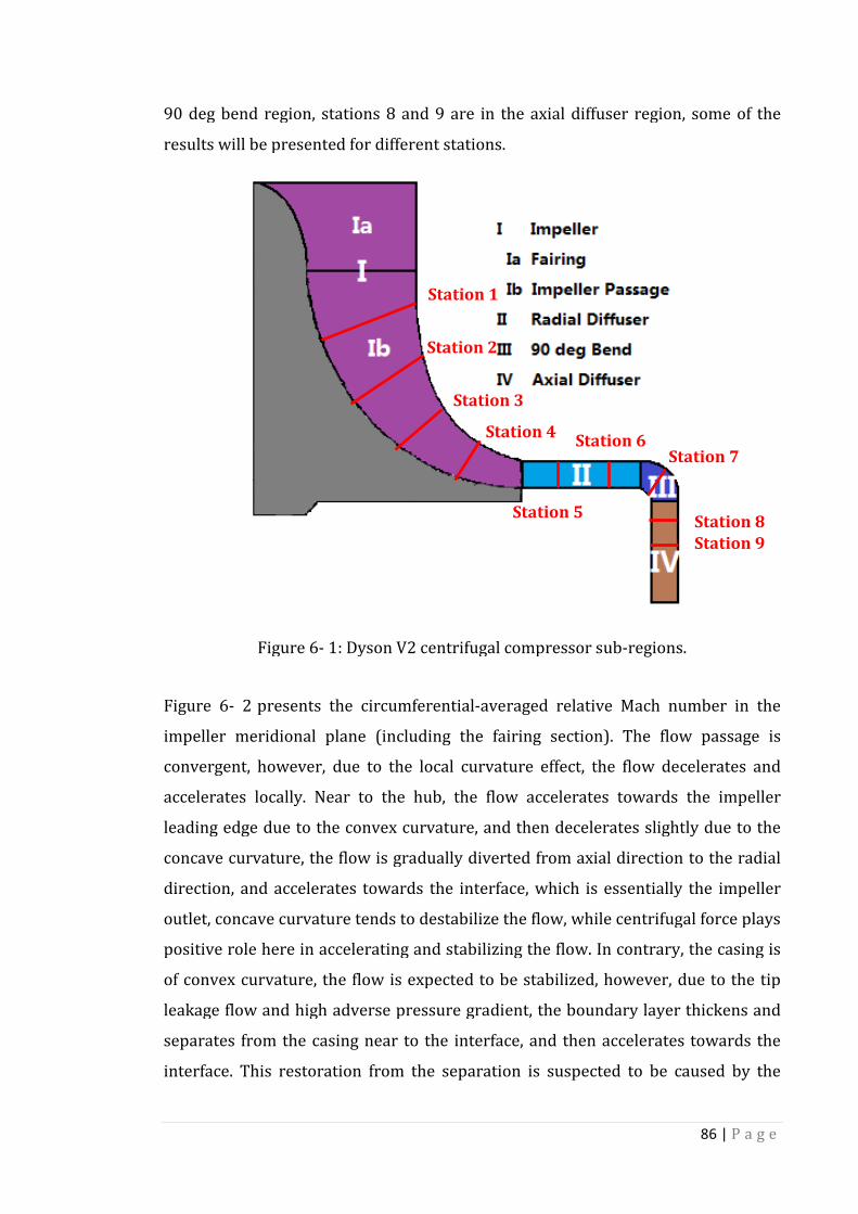
90 deg bend region, stations
results will be presented for different stations.
Figure 6
Figure 6- 2 presents the circumferential
impeller meridional plane (including the fairing section). The flow passage is
convergent, however, due to the local curvatur
accelerates locally. Near to the hub, the flow accelerates towards the impeller
leading edge due to the
concave curvature, the flow is gradually diverted from axi
direction, and accelerates towards the interface, which is essentially the impeller
outlet, concave curvature tends to destabilize the flow, while centrifugal force plays
positive role here in accelerating and stabilizing the flo
of convex curvature, the flow is expected to be stabilized, however, due to the tip
leakage flow and high adverse pressure gradient, the boundary layer thickens and
separates from the casing near to the interface, and then acc
interface. This restoration from the separation is suspected to be caused by the
90 deg bend region, stations 8 and 9 are in the axial diffuser region,
results will be presented for different stations.
Figure 6- 1: Dyson V2 centrifugal compressor sub
presents the circumferential-averaged relative Mach number in the
impeller meridional plane (including the fairing section). The flow passage is
convergent, however, due to the local curvature effect, the flow decelerates and
accelerates locally. Near to the hub, the flow accelerates towards the impeller
leading edge due to the convex curvature, and then decelerates slightly due to the
concave curvature, the flow is gradually diverted from axial direction to the radial
direction, and accelerates towards the interface, which is essentially the impeller
outlet, concave curvature tends to destabilize the flow, while centrifugal force plays
positive role here in accelerating and stabilizing the flow. In contrary, the casing is
of convex curvature, the flow is expected to be stabilized, however, due to the tip
leakage flow and high adverse pressure gradient, the boundary layer thickens and
separates from the casing near to the interface, and then acc
interface. This restoration from the separation is suspected to be caused by the
Station 1
Station 2
Station 3
Station 4
Station 5
Station
86 | P a g e
8 and 9 are in the axial diffuser region, some of the
: Dyson V2 centrifugal compressor sub-regions.
averaged relative Mach number in the
impeller meridional plane (including the fairing section). The flow passage is
e effect, the flow decelerates and
accelerates locally. Near to the hub, the flow accelerates towards the impeller
convex curvature, and then decelerates slightly due to the
al direction to the radial
direction, and accelerates towards the interface, which is essentially the impeller
outlet, concave curvature tends to destabilize the flow, while centrifugal force plays
w. In contrary, the casing is
of convex curvature, the flow is expected to be stabilized, however, due to the tip
leakage flow and high adverse pressure gradient, the boundary layer thickens and
separates from the casing near to the interface, and then accelerates towards the
interface. This restoration from the separation is suspected to be caused by the
Station 6 Station 7
Station 8
Station 9
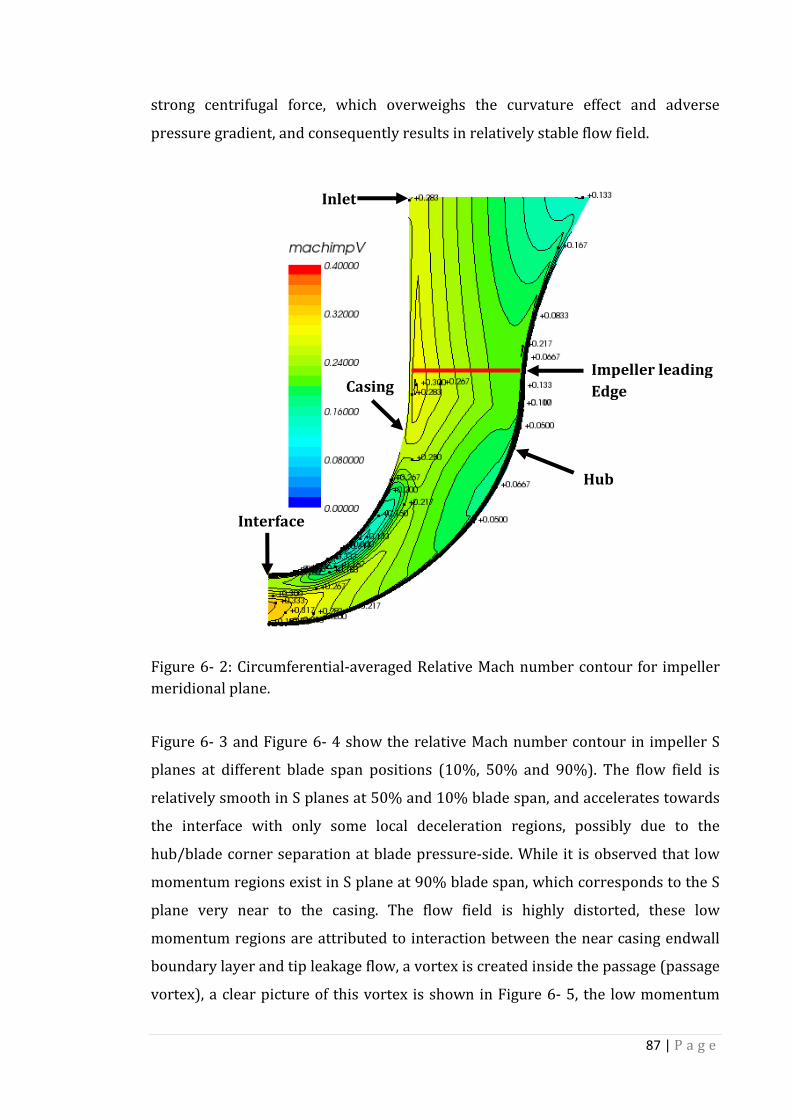
87 | P a g e
strong centrifugal force, which overweighs the curvature effect and adverse
pressure gradient, and consequently results in relatively stable flow field.
Figure 6- 2: Circumferential-averaged Relative Mach number contour for impeller
meridional plane.
Figure 6- 3 and Figure 6- 4 show the relative Mach number contour in impeller S
planes at different blade span positions (10%, 50% and 90%). The flow field is
relatively smooth in S planes at 50% and 10% blade span, and accelerates towards
the interface with only some local deceleration regions, possibly due to the
hub/blade corner separation at blade pressure-side. While it is observed that low
momentum regions exist in S plane at 90% blade span, which corresponds to the S
plane very near to the casing. The flow field is highly distorted, these low
momentum regions are attributed to interaction between the near casing endwall
boundary layer and tip leakage flow, a vortex is created inside the passage (passage
vortex), a clear picture of this vortex is shown in Figure 6- 5, the low momentum
Inlet
Interface
Casing
Hub
Impeller leading
Edge
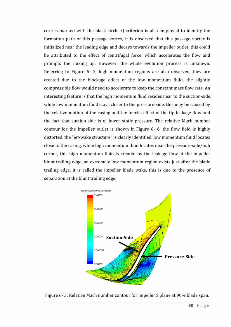
88 | P a g e
core is marked with the black circle. Q-criterion is also employed to identify the
formation path of this passage vortex, it is observed that this passage vortex is
initialized near the leading edge and decays towards the impeller outlet, this could
be attributed to the effect of centrifugal force, which accelerates the flow and
prompts the mixing up. However, the whole evolution process is unknown.
Referring to Figure 6- 3, high momentum regions are also observed, they are
created due to the blockage effect of the low momentum fluid, the slightly
compressible flow would need to accelerate to keep the constant mass flow rate. An
interesting feature is that the high momentum fluid resides near to the suction-side,
while low momentum fluid stays closer to the pressure-side, this may be caused by
the relative motion of the casing and the inertia effect of the tip leakage flow and
the fact that suction-side is of lower static pressure. The relative Mach number
contour for the impeller outlet is shown in Figure 6- 6, the flow field is highly
distorted, the "jet-wake structure" is clearly identified, low momentum fluid locates
close to the casing, while high momentum fluid locates near the pressure-side/hub
corner, this high momentum fluid is created by the leakage flow at the impeller
blunt trailing edge, an extremely low momentum region exists just after the blade
trailing edge, it is called the impeller blade wake, this is due to the presence of
separation at the blunt trailing edge,
Figure 6- 3: Relative Mach number contour for impeller S plane at 90% blade span.
Suction-Side
Pressure-Side

89 | P a g e
Figure 6- 4: Relative Mach number contour for impeller S planes at a) 10%, b) 50%
blade span.
Figure 6- 5: Relative velocity contour on four streamwise stations with streamlines.
Figure 6- 6: Relative Mach number contour for impeller outlet.
(a) (b)
Casing
Hub Blade Suction-Side Pressure-Side

90 | P a g e
Low momentum regions are observed to exist inside the passage, in order to have
more information about these regions, relative velocity contour on stations 1 to 4
are shown in Figure 6- 7, low momentum and high momentum regions are
observed and corresponding to those in Figure 6- 3. The premature "jet-wake
structure" is very different from that in Figure 6- 6 and similar to that in Figure 6- 3
and Figure 6- 4. The huge difference may be caused by the impeller trailing edge
leakage flow and impeller-diffuser interaction. The tip leakage flow is observed to
separate from the blade pressure-side and leak to the suction-side without
reattachment, possibly due to the very thin blade tip. It is also noted that, although
the vortex decays towards the impeller outlet, the low momentum region actually
increases in extent, possibly due to the roll-up effect of the vortex. Another distinct
feature is that the extent of the tip leakage flow increases towards the impeller
outlet, this is attributed to the increase in relative tip clearance size, which is
defined as the ratio of local tip clearance to the local blade span, the increase in
pressure difference between pressure-side and suction-side also plays a role here.
Figure 6- 7: Relative velocity contour on stations 1 to 4.
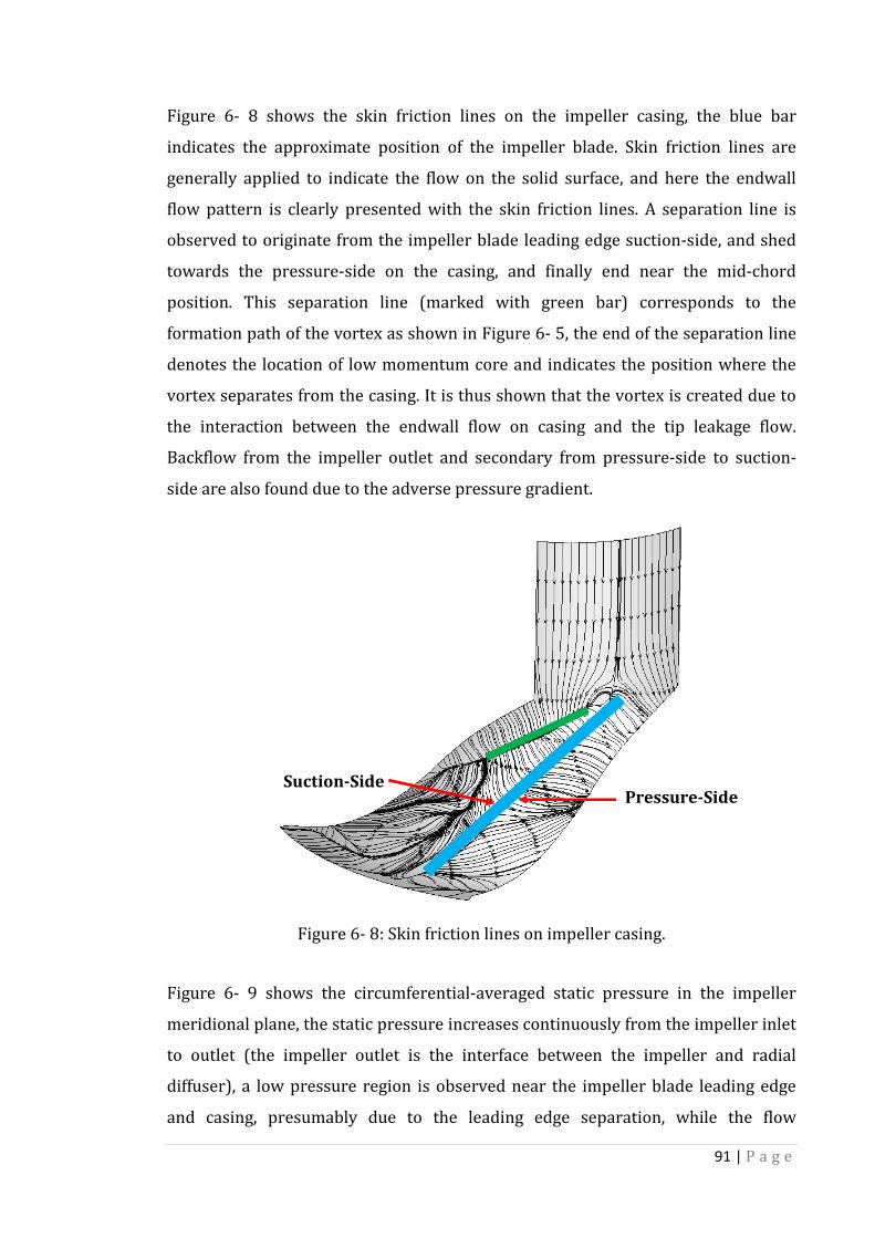
91 | P a g e
Figure 6- 8 shows the skin friction lines on the impeller casing, the blue bar
indicates the approximate position of the impeller blade. Skin friction lines are
generally applied to indicate the flow on the solid surface, and here the endwall
flow pattern is clearly presented with the skin friction lines. A separation line is
observed to originate from the impeller blade leading edge suction-side, and shed
towards the pressure-side on the casing, and finally end near the mid-chord
position. This separation line (marked with green bar) corresponds to the
formation path of the vortex as shown in Figure 6- 5, the end of the separation line
denotes the location of low momentum core and indicates the position where the
vortex separates from the casing. It is thus shown that the vortex is created due to
the interaction between the endwall flow on casing and the tip leakage flow.
Backflow from the impeller outlet and secondary from pressure-side to suction-
side are also found due to the adverse pressure gradient.
Figure 6- 8: Skin friction lines on impeller casing.
Figure 6- 9 shows the circumferential-averaged static pressure in the impeller
meridional plane, the static pressure increases continuously from the impeller inlet
to outlet (the impeller outlet is the interface between the impeller and radial
diffuser), a low pressure region is observed near the impeller blade leading edge
and casing, presumably due to the leading edge separation, while the flow
Suction-Side Pressure-Side
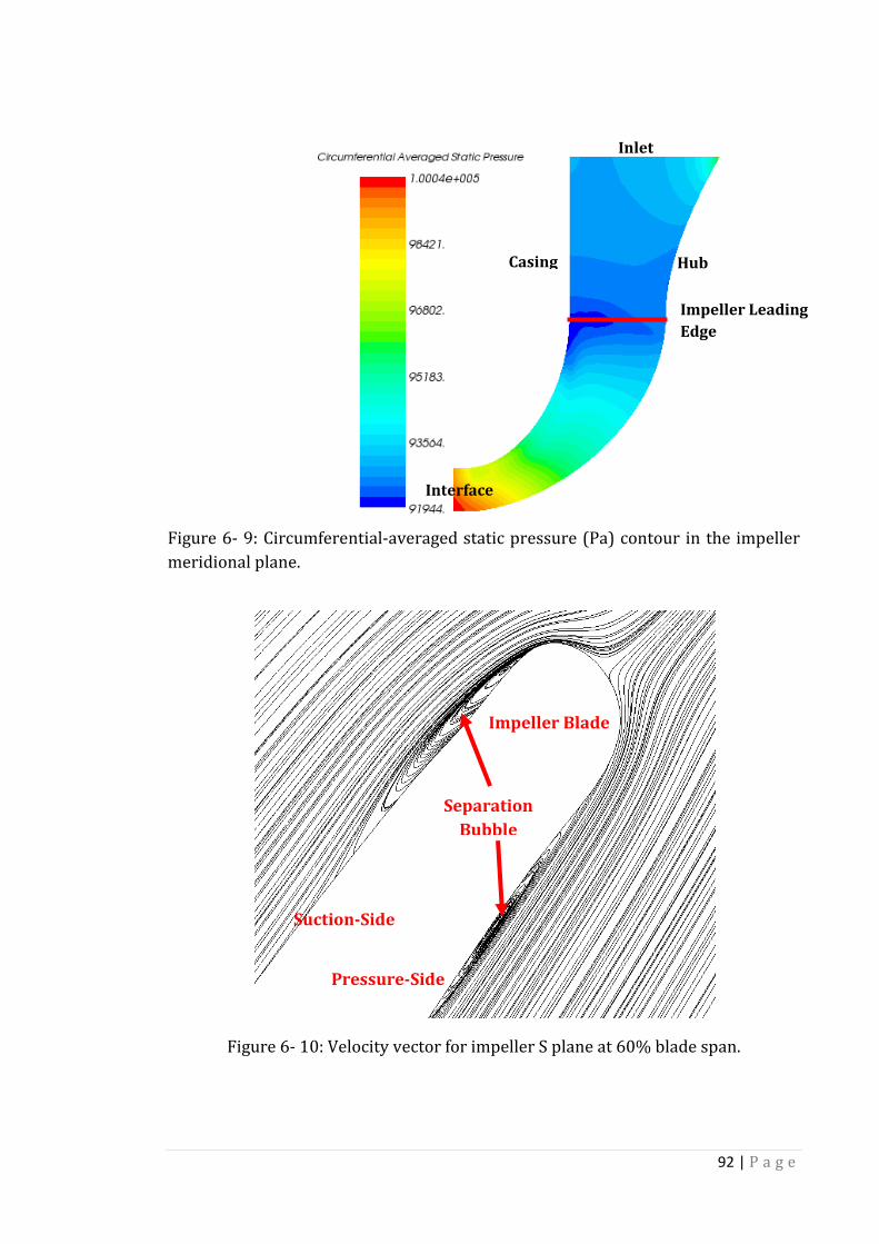
92 | P a g e
Figure 6- 9: Circumferential-averaged static pressure (Pa) contour in the impeller
meridional plane.
Figure 6- 10: Velocity vector for impeller S plane at 60% blade span.
Inlet
Hub Casing
Impeller Leading
Edge
Interface
Impeller Blade
Separation
Bubble
Pressure-Side
Suction-Side
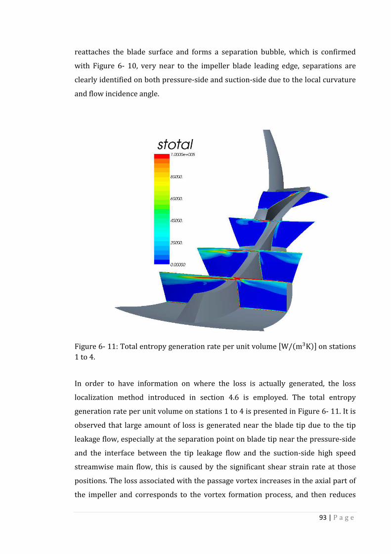
93 | P a g e
reattaches the blade surface and forms a separation bubble, which is confirmed
with Figure 6- 10, very near to the impeller blade leading edge, separations are
clearly identified on both pressure-side and suction-side due to the local curvature
and flow incidence angle.
Figure 6- 11: Total entropy generation rate per unit volume �W/�m�K�� on stations
1 to 4.
In order to have information on where the loss is actually generated, the loss
localization method introduced in section 4.6 is employed. The total entropy
generation rate per unit volume on stations 1 to 4 is presented in Figure 6- 11. It is
observed that large amount of loss is generated near the blade tip due to the tip
leakage flow, especially at the separation point on blade tip near the pressure-side
and the interface between the tip leakage flow and the suction-side high speed
streamwise main flow, this is caused by the significant shear strain rate at those
positions. The loss associated with the passage vortex increases in the axial part of
the impeller and corresponds to the vortex formation process, and then reduces

towards the impeller outlet
previously. The endwall loss and
impeller outlet due to the high flow velocity
Figure 6- 12 illustrates the hub endwall flow and the im
with the help of skin friction lines. It is observed that the hub endwall flow is in the
streamwise direction before the blade leading edge and
The blade surface flo
flows are caused by the pressure gradient and centrifugal force. However, the
centrifugal force also helps to overcome the
impeller outlet. Wall shear stress increases towards the impeller outle
increase in flow velocity. The high wall shear
entropy generation as giv
Figure 6- 12: Wall shear stress
blade and hub (a) suction
The outflow from the impeller goes into the radial diffuser as the inlet condition,
radial diffuser is very critical to the stage performance, the highly distorted flow
field may impact the radial diffuser performance significantly due to blockage at
the throat and stall inception. The radial diffuser blade sections
(a)
towards the impeller outlet possibly due to the decay of the vortex as described
he endwall loss and blade surface loss become significant
due to the high flow velocity.
illustrates the hub endwall flow and the impeller blade surface flow
with the help of skin friction lines. It is observed that the hub endwall flow is in the
streamwise direction before the blade leading edge and near to
he blade surface flow almost goes radially towards the blade tip.
flows are caused by the pressure gradient and centrifugal force. However, the
centrifugal force also helps to overcome the adverse pressure gradient near the
impeller outlet. Wall shear stress increases towards the impeller outle
increase in flow velocity. The high wall shear stress regions correspond
entropy generation as given in Figure 6- 11.
Wall shear stress (Pa) contour with skin friction lines on impeller
blade and hub (a) suction-side, (b) pressure-side.
outflow from the impeller goes into the radial diffuser as the inlet condition,
al diffuser is very critical to the stage performance, the highly distorted flow
field may impact the radial diffuser performance significantly due to blockage at
and stall inception. The radial diffuser blade sections
(b)
94 | P a g e
due to the decay of the vortex as described
become significant near the
peller blade surface flow
with the help of skin friction lines. It is observed that the hub endwall flow is in the
near to the impeller outlet.
blade tip. These secondary
flows are caused by the pressure gradient and centrifugal force. However, the
pressure gradient near the
impeller outlet. Wall shear stress increases towards the impeller outlet due to the
stress regions correspond to high
kin friction lines on impeller
outflow from the impeller goes into the radial diffuser as the inlet condition,
al diffuser is very critical to the stage performance, the highly distorted flow
field may impact the radial diffuser performance significantly due to blockage at
and stall inception. The radial diffuser blade sections in spanwise

95 | P a g e
direction would experience different inflow incidence angles, as a result, local
separation may occur. Figure 6- 13 shows the Mach number contour for diffuser S
planes at three spanwise positions, 10%, 50% and 90% respectively. Referring to
part (a), flow separation is observed at both pressure-side and suction-side in
radial diffuser, large regions of low momentum exist particularly inside the 90 deg
bend and axial diffuser. Part (b) shows large region of separation only in the axial
diffuser. In part (c), early flow separation is observed at suction-side of radial
diffuser blade, trailing edge separation is found inside the axial diffuser. The flow
separation can be attributed to boundary layer interaction at corner, adverse
pressure gradient due to large curvature, and more importantly, the highly
distorted inflow condition.
Figure 6- 13: Mach number contour for radial and axial diffusers S planes at (a) 10%
span, (b) 50% span, (c) 90% span.
Figure 6- 14 shows the incidence angle for the radial diffuser blade section at
different span locations, 10%, 50% and 90% respectively. The dashed box shows
the region of interest, because the incidence angle is generally defined for the
upstream. It is found that the incidence angle is negative for the blade section at 10%
span, and this blade section is subject to pressure-side separation, the situation is
very similar to the case of high mass flow rate operation, while for the blade section
at 90% span, the incidence angle is positive, suction-side separation occurs at mid-
(a) (b) (c)
Pressure-Side
Suction-Side

96 | P a g e
Figure 6- 14: Incidence angle (deg) contour for radial diffuser at (a) 10%, (b) 50%,
(c) 90% blade span.
Interface
Interface
Interface
Pressure-Side
Suction-Side
Pressure-Side
Pressure-Side
Suction-Side
Suction-Side
(a)
(b)
(c)

97 | P a g e
chord position, resembles the low mass flow rate operation. Only the blade section
at 50% span works relatively efficiently. As a whole, it can be imaged that the radial
diffuser is actually not very efficient, and perform badly even at near design
operation condition (stage).
Figure 6- 15: Total entropy generation rate per unit volume �W/�m�K�� on stations
5 to 9.
Figure 6- 15 shows the total entropy generation rate per unit volume on stations 5
to 9. Relatively high local loss generation is observed at both blade suction-side and
pressure-side in radial diffuser due to the flow separation, similar high local loss
generation is also observed at the axial diffuser suction-side. Hub endwall loss is
significant near the radial diffuser inlet, while it is difficult to distinguish the blade
surface loss from the separation induced loss.
The circumferential-averaged static pressure contour for the radial diffuser and
axial diffuser is shown in Figure 6- 16, very low pressure region is observed near
the interface due to the "jet-wake structure" from the impeller and previously
mentioned severe separation at the radial diffuser blade. High pressure region is
observed at the outer side the 90 deg bend, while low pressure region is observed
at the inner side the 90 deg bend, this is due to the presence of centrifugal force
induced pressure gradient.
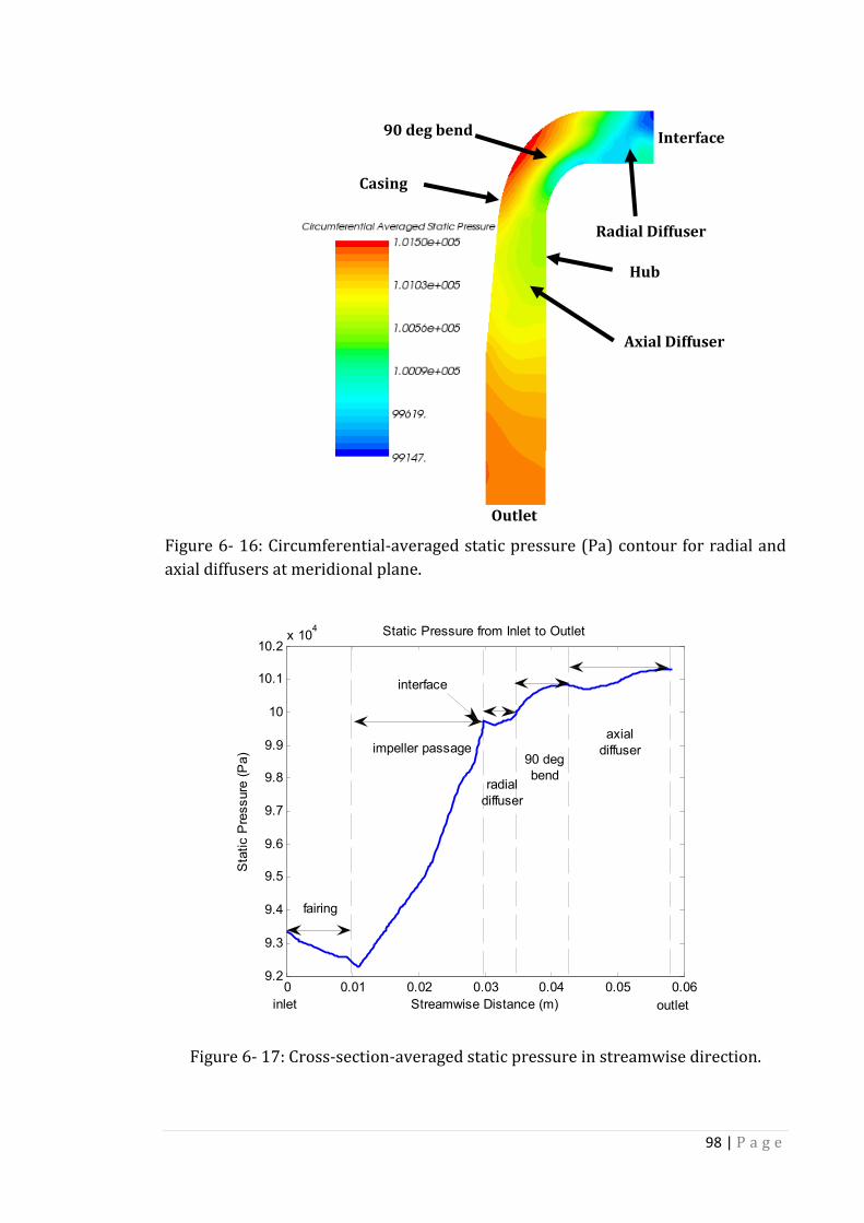
98 | P a g e
Figure 6- 16: Circumferential-averaged static pressure (Pa) contour for radial and
axial diffusers at meridional plane.
Figure 6- 17: Cross-section-averaged static pressure in streamwise direction.
0 0.01 0.02 0.03 0.04 0.05 0.069.2
9.3
9.4
9.5
9.6
9.7
9.8
9.9
10
10.1
10.2x 10
4
Streamwise Distance (m)
Sta
tic P
ressure
(P
a)
Static Pressure from Inlet to Outlet
inlet
interface
radial
diffuser
90 deg
bend
axial
diffuser
outlet
fairing
impeller passage
Interface
Hub
Casing
Radial Diffuser
Axial Diffuser
Outlet
90 deg bend

99 | P a g e
Figure 6- 17 shows the cross-section-averaged static pressure plotted in the
streamwise direction from compressor inlet to outlet, including fairing, impeller
passage, radial diffuser, 90 deg bend and axial diffuser. It is observed that the static
pressure drops in the fairing region, which is essentially a convergent section, the
flow field is only slightly affected by the rotating hub via the skin frication, and it
dips slightly after the impeller leading edge due to the previous mentioned leading
edge separation bubble. After that, the static pressure rises continuously towards
the impeller outlet, a striking feature is that almost 80% of the static pressure
arises from the impeller. The static pressure only increases slightly in the radial
diffuser due to the highly distorted inflow condition, the diffuser blade cannot
recover the static pressure efficiently, very similar situation is observed for axial
diffuser, except the impeller, the 90 deg bend contributes the greatest to the static
pressure rise. In total, this plot shows that the diffusers are actually not designed to
work efficiently under the highly distorted inflow condition.
6.3. Summary
The flow field inside the Dyson V2 centrifugal compressor was analysed in this
chapter using steady simulation, with the impeller operating at design condition
(Case 1), while the whole stage operated at near design operation condition.
Distinct flow features were observed, such as tip leakage flow, separation bubble,
the so called "jet-wake structure" and corner separation. The vortex roll-up process
was identified, the tip leakage flow from the impeller leading edge plays the role of
initializing the vortex roll-up, tip leakage flow from the first half of the impeller
blade chord contributes to the formation of the vortex, while that from the rest of
the blade chord plays an important role in the decay of the vortex, severe blockage
and loss are associated with the vortex inside the passage. Towards the impeller
outlet, the vortex decays presumably due to the accelerating effect of centrifugal
force. The main mechanisms for loss generation were identified, tip leakage flow is
the most significant source of loss generation in impeller, it induces losses from
both vortex roll-up and blade tip high shear flow, in general, tip leakage flow is
difficult to control and cannot be avoided. Endwall loss and blade surface loss also
contribute to the loss generation in impeller, especially in the regions near the

100 | P a g e
impeller outlet. The losses in both radial diffuser and axial diffuser can be
summarised as endwall loss, blade surface loss and separation induced loss. In this
work, riblets is proposed to reduce the endwall loss on the impeller hub, the wall
shear stress predicted with steady simulation will be used to design the riblets in
chapter 8. The diffuser inflow condition is primarily characterized by the highly
distorted flow, which makes the diffuser work very inefficiently, as a result, only
about 8% of the static pressure rise is obtained through the diffuser. while the
impeller accounts for about 80% of the static pressure rise due to the effect of
centrifugal force. The current results suggest that the inflow condition into the
diffuser may be improved to increase the diffuser performance.

101 | P a g e
Chapter 7 Effects of Unsteadiness
Effects of Unsteadiness
7.1. Introduction
Flow analysis has been conducted in the last chapter through single passage steady
simulation. The general flow features have been discussed. However, it is well
known that the flow inside a centrifugal compressor is highly unsteady, steady
simulation would not be able to take into account the unsteadiness, thus the results
may be not that accurate. Therefore, it is essential to examine to what extent this
unsteadiness would affect the centrifugal compressor flow field. This chapter
intends to analyse the effect of unsteadiness on the performance and flow field of
Dyson V2 centrifugal compressor. The simulation conditions are very similar to
those of ERCOFTAC centrifugal compressor as presented in section 5.4, and the
unsteady flow field analysis is limited to the impeller design operation condition
Case 1.
7.2. Results
It is generally useful to compare the performance prediction results between
steady simulation and unsteady simulation, performance is the direct reflection of
the flow field, so the difference in performance would imply the existence of
different predicted flow behaviours. Figure 7- 1 presents the performance
predictions from steady and unsteady simulations, it is found that unsteady
simulation tends to predict the performance with higher values. It is known that
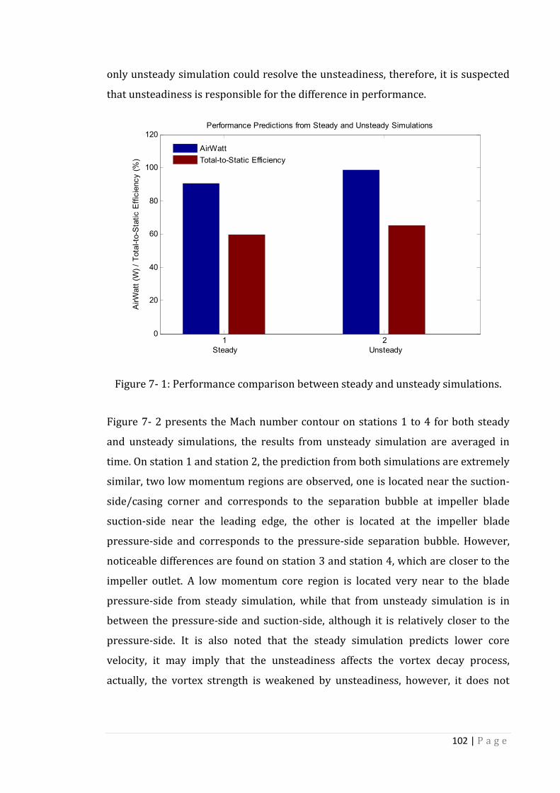
102 | P a g e
only unsteady simulation could resolve the unsteadiness, therefore, it is suspected
that unsteadiness is responsible for the difference in performance.
Figure 7- 1: Performance comparison between steady and unsteady simulations.
Figure 7- 2 presents the Mach number contour on stations 1 to 4 for both steady
and unsteady simulations, the results from unsteady simulation are averaged in
time. On station 1 and station 2, the prediction from both simulations are extremely
similar, two low momentum regions are observed, one is located near the suction-
side/casing corner and corresponds to the separation bubble at impeller blade
suction-side near the leading edge, the other is located at the impeller blade
pressure-side and corresponds to the pressure-side separation bubble. However,
noticeable differences are found on station 3 and station 4, which are closer to the
impeller outlet. A low momentum core region is located very near to the blade
pressure-side from steady simulation, while that from unsteady simulation is in
between the pressure-side and suction-side, although it is relatively closer to the
pressure-side. It is also noted that the steady simulation predicts lower core
velocity, it may imply that the unsteadiness affects the vortex decay process,
actually, the vortex strength is weakened by unsteadiness, however, it does not
1 20
20
40
60
80
100
120A
irW
att
(W
) /
Tota
l-to
-Sta
tic E
ffic
iency (
%)
Performance Predictions from Steady and Unsteady Simulations
AirWatt
Total-to-Static Efficiency
Steady Unsteady

103 | P a g e
Figure 7- 2: Relative Mach number contour for steady and unsteady simulations on
stations 1 to 4 (top to bottom) in impeller region.
Time-Averaged Unsteady Simulation Steady Simulation

104 | P a g e
Figure 7- 3: Mach number contour for steady and unsteady simulations on stations
5 to 9 (top to bottom) in diffuser region.
Steady Simulation Time-Averaged Unsteady Simulation
105 | P a g e
have noticeable effects on the vortex formation process, and the unsteadiness may
be primarily resulted from the impeller-diffuser interaction.
The diffuser Mach number contours predicted from both steady and unsteady
simulations are compared in Figure 7- 3 on stations 5 to 9, Low momentum regions
are observed across all stations. The low momentum regions should correspond to
separations as discussed before. Steady simulation predicts relatively large regions
of low momentum fluid compared to prediction from unsteady simulation, the
difference between them increases towards the diffuser outlet. The difference may
imply that unsteadiness could essentially prompt momentum exchange and help
weaken or suppress the flow separation, it may be concluded that the blockage is
reduced inside the diffuser passage due to the unsteadiness.
Referring to Figure 7- 4, the local entropy generation rate contours are presented
on station 4 (impeller) and station 6 (diffuser) for different time instant (non-
dimensionalised according to Eqn 5-1), comparison is also made between steady
and unsteady simulations. On station 4, steady and unsteady simulations give
different predictions on tip leakage flow induced local loss generation. It is obvious
that steady simulation over-predicts the local loss generation, unsteadiness seems
to weaken the tip leakage flow induced vortex. Similarly, steady simulation over-
predicts the local loss generation on station 6, unsteadiness seems to weaken or
suppress the flow separation in diffuser. At different time instants, the local loss
contour only varies slightly, the effect of unsteadiness is very limited on station 4
and station 6.
As mentioned before, the unsteadiness generated by impeller-diffuser interaction is
significant at positions near the impeller outlet. To understand the effects of
impeller-diffuser interaction, Relative Mach number contours at different time
instants are presented in Figure 7- 5, the black bar indicates the position of radial
diffuser leading edge, the black trapezoid represents the position of the impeller
blade trailing edge. The impeller blade moves to the right, while the diffuser blade
is stationary. Two distinct features are observed, the first one is that the presence
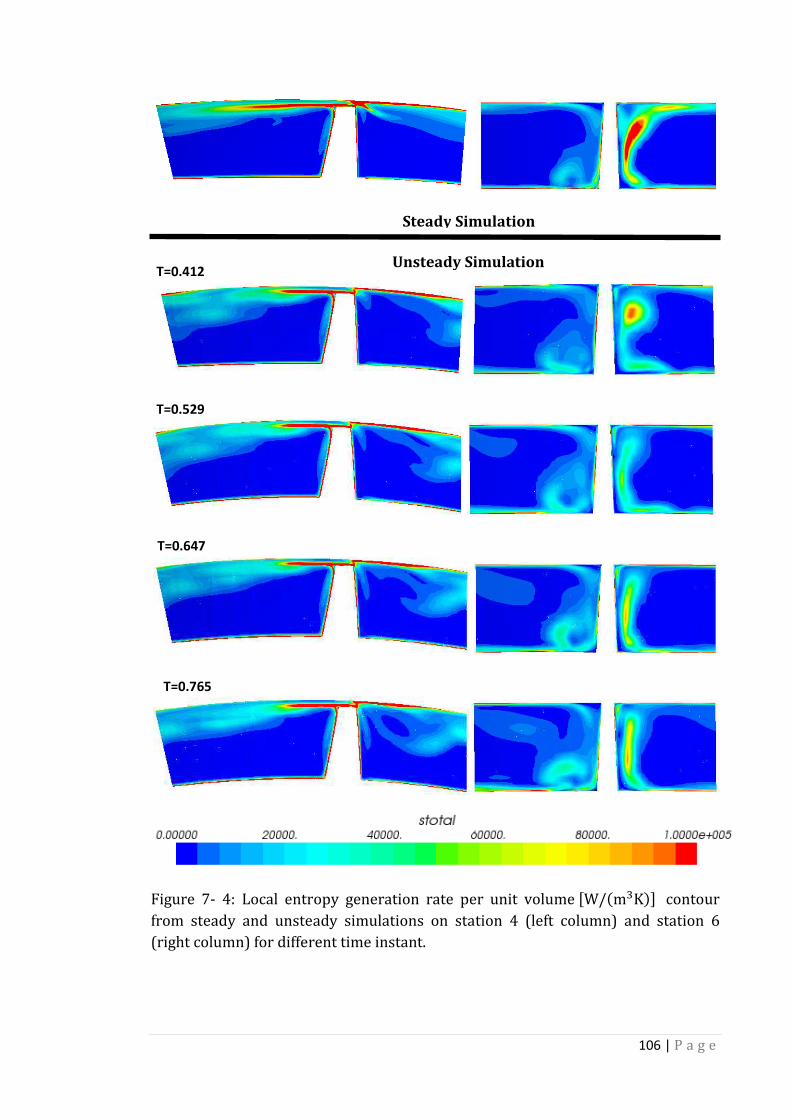
106 | P a g e
Figure 7- 4: Local entropy generation rate per unit volume �W/�m�K�� contour
from steady and unsteady simulations on station 4 (left column) and station 6
(right column) for different time instant.
Steady Simulation
Unsteady Simulation T=0.412
T=0.529
T=0.647
T=0.765
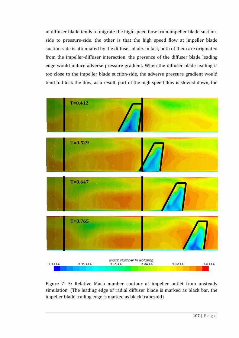
107 | P a g e
of diffuser blade tends to migrate the high speed flow from impeller blade suction-
side to pressure-side, the other is that the high speed flow at impeller blade
suction-side is attenuated by the diffuser blade. In fact, both of them are originated
from the impeller-diffuser interaction, the presence of the diffuser blade leading
edge would induce adverse pressure gradient. When the diffuser blade leading is
too close to the impeller blade suction-side, the adverse pressure gradient would
tend to block the flow, as a result, part of the high speed flow is slowed down, the
Figure 7- 5: Relative Mach number contour at impeller outlet from unsteady
simulation. (The leading edge of radial diffuser blade is marked as black bar, the
impeller blade trailing edge is marked as black trapezoid)
T=0.412
T=0.529
T=0.647
T=0.765
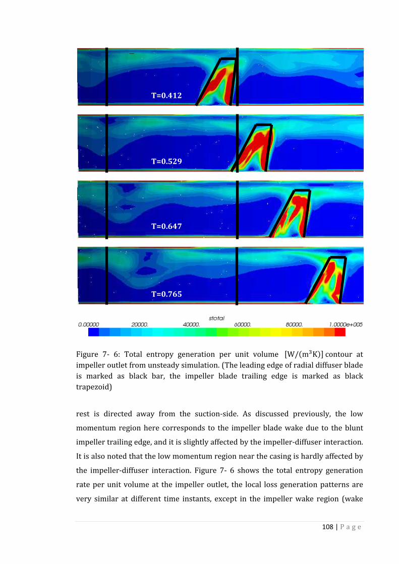
108 | P a g e
Figure 7- 6: Total entropy generation per unit volume �W/�m�K�� contour at
impeller outlet from unsteady simulation. (The leading edge of radial diffuser blade
is marked as black bar, the impeller blade trailing edge is marked as black
trapezoid)
rest is directed away from the suction-side. As discussed previously, the low
momentum region here corresponds to the impeller blade wake due to the blunt
impeller trailing edge, and it is slightly affected by the impeller-diffuser interaction.
It is also noted that the low momentum region near the casing is hardly affected by
the impeller-diffuser interaction. Figure 7- 6 shows the total entropy generation
rate per unit volume at the impeller outlet, the local loss generation patterns are
very similar at different time instants, except in the impeller wake region (wake
T=0.412
T=0.529
T=0.647
T=0.765
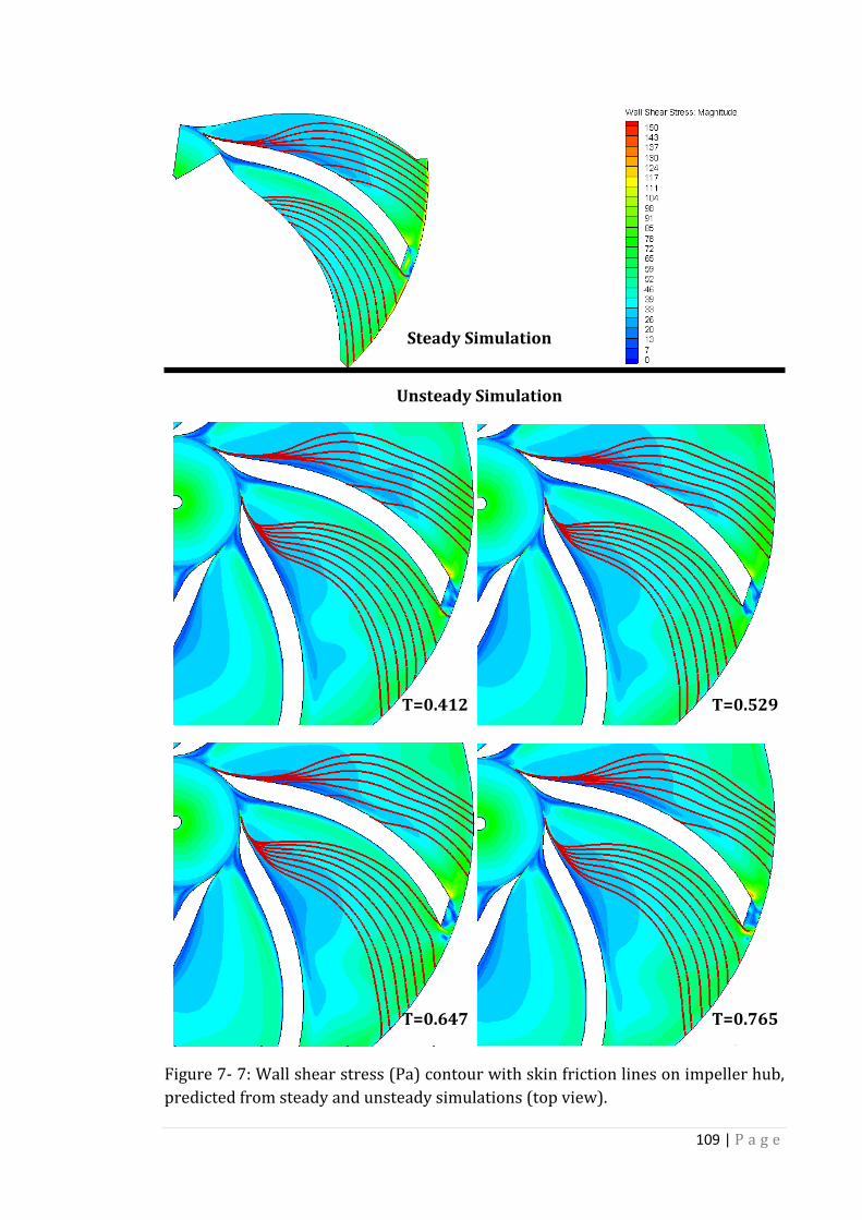
109 | P a g e
Figure 7- 7: Wall shear stress (Pa) contour with skin friction lines on impeller hub,
predicted from steady and unsteady simulations (top view).
Steady Simulation
Unsteady Simulation
T=0.529 T=0.412
T=0.647 T=0.765

110 | P a g e
loss), it is thus concluded that the impeller-diffuser interaction only slightly affect
the loss behaviour inside the impeller.
The wall shear stress contour with skin friction lines is presented in Figure 7- 7
from both steady and unsteady simulations. It is observed that the predicted wall
shear stresses and skin friction lines only differ slightly between steady and
unsteady simulations, perceivable variations are only found near the blade
pressure-side and could be attributed to the presence of a very weak vortex, which
may occur at the blade/hub junction due to boundary layer interaction.
7.3. Summary
Some of the important aspects of unsteadiness were discussed in this chapter,
unsteadiness was found to help improve performance. The underlying reason is
that unsteadiness would help weaken flow separation and associated vortex, as a
result, both blockage and local loss generation were reduced considerably.
Impeller-diffuser interaction had significant effects on the high speed flow at the
impeller blade suction-side, the radial diffuser leading edge migrated high speed
flow from impeller blade suction-side to pressure-side and slowed down the high
speed flow at impeller blade suction-side. However, it has limited effects on the tip
leakage flow induced passage vortex, the local loss generation was hardly affected.
The effects of unsteadiness on the hub wall shear stress distribution were
examined, both the magnitude and direction are changed slightly due to
unsteadiness. To assess whether riblets designed based on steady simulation
would perform acceptably in real operation, the effects of unsteadiness have to be
investigated.

111 | P a g e
Chapter 8 Application of Riblets
Application of Riblets
8.1. Introduction
This chapter presents the application of riblets. First of all, further topics on riblets
are discussed, including the riblets operation regimes, yaw-angle effect,
optimization of riblets and etc, only sawtooth riblets are considered due to the
availability of experimental data, an explicit expression is obtained to relate the
wall shear stress reduction to the riblets non-dimensional spacing. Then riblets are
proposed to be applied to the hub of Dyson V2 centrifugal compressor to help
reduce the hub endwall loss, steady simulation results have been used to design the
riblets. At the end, the effects of unsteadiness on riblets performance are discussed
to check whether the designed riblets could achieve acceptable performance in real
operation, for which the flow is essentially unsteady. And it should be noted that
this preliminary work is limited to the impeller design operation condition Case 1.
8.2. Further Discussions on Riblets
Riblets surface is extensively studied in literature, and it is generally referred to as
a kind of passive flow control method, which can manipulate the flow intentionally.
Riblets can be applied in two ways, either delaying the laminar-turbulent transition,
or reducing the skin friction drag in turbulent flow. Because the laminar-turbulent
transition itself is still an open question, and flow is almost all turbulent in nature,
most of the works on riblets have been focused on the turbulent skin friction drag

112 | P a g e
reduction. Here, attention has been paid to the turbulent skin friction drag
reduction with riblets.
Generally, wall shear stress reduction is used to assess the effectiveness of riblets,
wall shear stress reduction can be plotted against non-dimension spacing su to
obtain the riblets performance curve. In literature, it is found that the riblets
performance curve can be split into segments corresponding to different features,
as shown in Figure 8- 1, according to Bechert et al. (1997a), if su is small enough,
the viscous interaction is expected to be linear, as a result, the wall shear stress
reduction is nearly linearly proportional to su, however, when su increases, the
interaction becomes nonlinear, if su is large enough, the riblets will behave like a
rough surface. In practice, the 'viscous regime' is likely to be valid for su < 10~15
(Garcia-Mayoral and Jimenez, 2011), in the current work, a value of 10 is used to
separate the linear 'viscous regime' and the nonlinear interaction counterpart. The
expressions for wall shear stress reduction and su are given as Eqn 8-1.
Ö∆τ
τ�%� = Asu Ifsu ≤ 10∆τ
τ�%� = f�su� Ifsu > 10Û Eqn 8- 1
Where A is a constant and represents the slope, f�∎� is a nonlinear function and
obtained using nonlinear curve fitting.
Figure 8- 1: General structure of a wall shear stress reduction curve with riblets
(Bechert et al., 1997a).

As mentioned previously, sawtooth ribl
of experimental data in literature.
in this work is shown in
obtained from Walsh and Lindemann (1984) and plo
geometric parameter is required to define the riblets size, spacing is used in this
work. Curve fitting is employed to obtain the explicit
shear stress reduction and
The fitted curve is plotted in
fitting is good.
ò Af�
Curve fitting has been
stress reduction and riblets non
wall shear stress such that the riblets spacing can be calculated using Eqn 2
generally difficult to obta
Demont (1997) proposed to estimate the wall shear stress from the simple case of
turbulent flow over a flat plate, it is of general practice to apply momentum integral
equation to a 1/7 power velocity pr
As mentioned previously, sawtooth riblets will be employed due to the availability
of experimental data in literature. The specific sawtooth riblets configuration used
shown in Figure 8- 2, the corresponding experimental data are
obtained from Walsh and Lindemann (1984) and plotted in Figure 8
geometric parameter is required to define the riblets size, spacing is used in this
urve fitting is employed to obtain the explicit expression
shear stress reduction and non-dimensional spacing su, as given in Eqn 8
curve is plotted in Figure 8- 3, it is noted that the
A ! 73.7778E 7 1�su� ! �3.8959E 7 6��su�� 7 �5.9223E 7 4
7�6.7087E 7 1��su� D �1.6160
Figure 8- 2: Sawtooth riblets dimensions.
Curve fitting has been conducted to obtain the relationship between wall shear
stress reduction and riblets non-dimensional spacing, the next step is to obtain the
wall shear stress such that the riblets spacing can be calculated using Eqn 2
generally difficult to obtain the wall shear stress. Anderson, Macgillivray and
Demont (1997) proposed to estimate the wall shear stress from the simple case of
turbulent flow over a flat plate, it is of general practice to apply momentum integral
equation to a 1/7 power velocity profile, and obtain:
113 | P a g e
ets will be employed due to the availability
The specific sawtooth riblets configuration used
the corresponding experimental data are
Figure 8- 3. Only one
geometric parameter is required to define the riblets size, spacing is used in this
expression between the wall
given in Eqn 8-2 below.
, it is noted that the quality of the curve
4��su��
6160E 7 2�
Û Eqn 8- 2
.
conducted to obtain the relationship between wall shear
dimensional spacing, the next step is to obtain the
wall shear stress such that the riblets spacing can be calculated using Eqn 2-19. It is
in the wall shear stress. Anderson, Macgillivray and
Demont (1997) proposed to estimate the wall shear stress from the simple case of
turbulent flow over a flat plate, it is of general practice to apply momentum integral

114 | P a g e
Figure 8- 3: Wall shear stress reduction for sawtooth riblets obtained from Walsh
and Lindemann (1984) with curve fitting.
τs = "� ρU� �.��ô�¦àõ(/ö Eqn 8- 3
Where ReJ = HJ� , x is the distance measured from the leading edge, U is the flow
velocity over the surface.
However, in the case of compressor, due to the complex geometry and flow
behaviour involved, Eqn 8-3 is unlikely to give acceptable prediction on wall shear
stress. Therefore, wall shear stress is obtained from numerical simulation in this
work.
As already discussed in 2.4.1, riblets is subject to performance deterioration under
yaw-angle effect, and the flow in practical application is seldom aligned with one
fixed direction, instead, the flow direction varies. As a result, yaw-angle effect is
needed to be considered carefully to ensure that the riblets performance is not
severe impacted. In literature, only a few experimental data on yaw-angle effect are
available. Those of Walsh and Lindemann (1984) are plotted in Figure 8- 4, wall
0 10 20 30 40 50 60-10
-8
-6
-4
-2
0
2
4
6
8
10
s+
△τ/
τ (%
)
Wall Shear Stress Reduction for Sawtooth Riblets
Walsh & Lindemann, 1984
Curve Fitting

115 | P a g e
shear stress reduction data are available for three different yaw angles, 0 deg, 15
deg and 30 deg respectively, curve fitting is performed for each set of data, the
corresponding fitted curve is plotted as well, a summary of the nonlinear curve
fitting is given in Table 8- 1, polynomials of different orders are applied to obtain
the most appropriate curve fitting. Although the explicit expressions for three yaw
angles are available, the intermediate values cannot be obtained directly. A
nonlinear interpolation (quadratic) is applied to relate the wall shear stress
reduction to the yaw-angle at constant non-dimensional spacing. As a result, the
Figure 8- 4: Yaw-angle effect on riblets performance with data cited from Walsh
and Lindemann (1984).
wall shear stress reduction can be expressed in terms of non-dimensional spacing
and yaw-angle, and given as:
∆τ
τ�%� = f"�su�ψ� + f��su�ψ + f��su� Eqn 8- 4
Where f" , f� and f� are functions of non-dimensional spacing and depend on
whether the riblets operate in the linear regime or nonlinear regime.
0 10 20 30 40 50 60-10
-5
0
5
10
15
20
25
30
35
40
s+
△τ/
τ (%
)
Yaw Angle Effect on Sawtooth Riblets Performance
0 Deg (Walsh & Lindemann, 1984)
0 Deg Curve Fitting
15 Deg (Walsh & Lindemann, 1984)
15 Deg Curve Fitting
30 Deg (Walsh & Lindemann, 1984)
30 Deg Curve Fitting

116 | P a g e
Riblets
Config.
Yaw
Angle
(deg)
Order Expression
Sawtooth
0 Quartic A"�su�� + B"�su�� + C"�su�� + D"su + ES"
15 Quartic AS��su�� + BS��su�� + CS��su�� + DS�su+ ES�
30 Quadratic AS��su�� + BS�su + CS�
Table 8- 1: A summary of the curve fitting for sawtooth riblets.
Figure 8- 5: Top view of the scallop shell. (Anderson, Macgillivray and Demont,
1997)
Figure 8- 6: Magnified view of scallop shell. (Anderson, Macgillivray and Demont,
1997)

117 | P a g e
In practical application, the surface to apply riblets may be convergent or divergent.
For instance, the impeller hub is actually divergent, the length in circumferential
direction increases towards the impeller outlet. If constant number of riblets are
applied, the riblets spacing will inevitably increase towards the divergent direction,
as a result, the riblets performance may be impacted. In nature, there are ways to
resolving this problem. Anderson, Macgillivray and Demont (1997) found that
scallop shells are covered with riblets to help reduce the turbulent skin friction
drag, as shown in Figure 8- 5, they estimated the wall shear stress with Eqn 8-3,
and concluded that riblets spacing should be smaller at the leading edge and
increases in the downstream direction. However, referring to Figure 8- 5, the
situation for scallop shells seem to be completely different. A magnified view
reveals the magic feature, as shown in Figure 8- 6, the black circles indicate the
newly added riblets. This feature is called intercalation, the newly added riblets
effectively reduce the riblets spacing towards the leading edge and maintain the
effectiveness of riblets at certain high level.
In literature, most of the experimental data on riblets are obtained with regard to
the average wall shear stress for the whole testing plate or tube and measured with
shear stress balance. The local wall shear is seldom measured due to the difficulty
in taking measurements locally, in this case, only indirect method can be applied,
for instance, Bechert et al. (1997a) applied Preston tube, which actually makes use
of a Pitot tube, to measure the wall shear stress distribution, Figure 8- 7 presents
the wall shear stress distribution on test plate (with riblets) and reference plate
(smooth) at two different Reynolds numbers as measured by Bechert et al., the wall
shear stress distributions for both plates are not uniform, compared to the
reference plate, the wall shear stress distribution for test plate shifts horizontally to
the left, indicating the existence of wall shear stress reduction, and it is found that
the wall shear stress reduction is nearly constant across the plate at both Reynolds
numbers, except at the upper corner of the test plate, this may be caused by the
presence of pressure gradient control. The experimental data used in this work are
the average wall shear stress as measured by Walsh and Lindemann (1984) in a
wind tunnel, in this preliminary study, it is assumed that the local wall shear stress
reduction distribution and local wall shear stress distribution are uniform for their

experiment, and thus the measured averaged wall shear stress reduction
treated as local quantity and corresponds to local wall shear stress in the following
studies.
Figure 8- 7: Wall shear stress distribution on test plate. (Bechert et al., 1997)
8.3. Riblets on Dyson V2 Impeller
Tremendous amount of effort
compressor performance, improvements have been achieved, however, most of
them are on operation range and operation stability, the reduction in loss
generation is seldom achieved, possibly due to the complex
involved. Dyson V2 centrifugal compressor is of small size, as a result, the flow
behaviour is even more complicated. As discussed previously, the tip leakage flow
in Dyson V2 impeller is the primary source of loss generation, the flow sepa
from the blade tip at the pressure
without reattachment due to the nature of the very thin blade tip, it is thus difficult
experiment, and thus the measured averaged wall shear stress reduction
as local quantity and corresponds to local wall shear stress in the following
: Wall shear stress distribution on test plate. (Bechert et al., 1997)
Riblets on Dyson V2 Impeller
Tremendous amount of efforts have been devoted to improving the centrifugal
compressor performance, improvements have been achieved, however, most of
them are on operation range and operation stability, the reduction in loss
generation is seldom achieved, possibly due to the complex
involved. Dyson V2 centrifugal compressor is of small size, as a result, the flow
behaviour is even more complicated. As discussed previously, the tip leakage flow
in Dyson V2 impeller is the primary source of loss generation, the flow sepa
from the blade tip at the pressure-side and generally leaks to the suction
without reattachment due to the nature of the very thin blade tip, it is thus difficult
118 | P a g e
experiment, and thus the measured averaged wall shear stress reduction can be
as local quantity and corresponds to local wall shear stress in the following
: Wall shear stress distribution on test plate. (Bechert et al., 1997)
s have been devoted to improving the centrifugal
compressor performance, improvements have been achieved, however, most of
them are on operation range and operation stability, the reduction in loss
generation is seldom achieved, possibly due to the complex flow behaviour
involved. Dyson V2 centrifugal compressor is of small size, as a result, the flow
behaviour is even more complicated. As discussed previously, the tip leakage flow
in Dyson V2 impeller is the primary source of loss generation, the flow separates
side and generally leaks to the suction-side
without reattachment due to the nature of the very thin blade tip, it is thus difficult
119 | P a g e
to control the tip leakage flow. Despite tip structures may help reduce the amount
of tip leakage flow slightly, the additional loss due to friction of these structures
usually overweighs the benefits. Endwall loss and blade surface loss are another
two sources of losses and affected by the skin friction drag, which is usually
characterized with the wall shear stress. In other words, the loss generation will be
less if the wall shear stress is reduced. Referring to Figure 6- 11, the hub endwall
loss near the impeller outlet is significant, the reduction in wall shear stress here
would result in significantly less loss generation. Riblets surface is proposed to
attack the problem in this work, due to the extremely high computational cost
involved in computing the flow field around riblets, curve fitting approach is
employed as introduced previously.
It is known that riblets should be designed properly, otherwise, they may work the
other way around and give rise to increase in wall shear stress. The flow field
prediction from steady simulation will be used to design the riblets. As mentioned
before, sawtooth riblets are employed here, so only three design aspects have to be
considered, i.e. riblets location, riblets orientation and riblets size. The application
of riblets should not prompt flow separation, so riblets should be applied to the
region where skin friction lines are directed towards and ended at the impeller
outlet. Referring to Figure 6- 12, it is noted that there is a region on the hub where
skin friction lines are properly directed, the flow in this region is expected to be
turbulent and free from separation. So it is determined that riblets will be applied
to this region on hub, as shown in Figure 8- 8 and marked with the circular band,
and the riblets are aligned with the skin friction lines such that the yaw-angle effect
is avoided in the context of steady simulation, however, due to the effect of
unsteadiness, yaw-angle effect cannot be avoided in the real operation, it will be
discussed in section 8.4. As shown in Figure 8- 2, the ratio of riblets height to
spacing is already known, so only riblets spacing has to be determined such that
the largest wall shear stress reduction can be achieved, in fact, it is an optimization
process. First of all, the wall shear stress distribution is extracted at discrete
circumferential stations, as shown in Figure 8- 9, here, only 15 stations are selected,
the stations are named from the pressure-side (station 1) to the suction-side
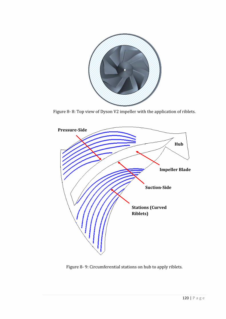
Figure 8- 8: Top view of Dyson V2 impeller
Figure 8
Pressure-Side
: Top view of Dyson V2 impeller with the application of riblets
Figure 8- 9: Circumferential stations on hub to apply riblets.
Impeller Blade
Side
Suction-Side
Stations (Curved
Riblets)
120 | P a g e
with the application of riblets.
: Circumferential stations on hub to apply riblets.
Impeller Blade
Side
Hub
Stations (Curved

121 | P a g e
Figure 8- 10: Wall shear stress distribution on 7 stations.
Figure 8- 11: Optimum riblets spacing on different stations.
0.004 0.006 0.008 0.01 0.012 0.014 0.016 0.0180
10
20
30
40
50
60
70
80
Distance from Rotation Axis (m)
Wall
Shear
Str
ess (
Pa)
Wall Shear Stress Distribution on 7 Stations
Station 2
Station 4
Station 6
Station 8
Station 10
Station 12
Station 14
Pressure-Side
Suction-Side
1 2 3 4 5 6 7 8 9 10 11 12 13 14 150
5
10
15
20
25
30
35
40
45
50
Station Number
Optim
um
Rib
lets
Spacin
g (
um
)
Optimum Riblets Spacing on Different Stations

122 | P a g e
Figure 8- 12: Maximum wall shear stress reduction on different stations.
(station 15). Optimization is conducted on each station with enumeration method.
In the future, more stations can be selected to represent the hub endwall more
accurately. The wall shear stress distributions for 7 stations are plotted in Figure 8-
10. The general trend for wall shear stress is observed that it increases from
pressure-side to suction-side due to the higher velocity at the suction side.
The riblets size has been optimized on each station, the optimum riblets spacing is
given in Figure 8- 11 for each station, it is found that the optimum spacings are all
around 35μm. The corresponding maximum wall shear stress reduction on each
station is plotted in Figure 8- 12, almost 4% wall shear stress reduction can be
achieved across all stations. In total, the spacing for the designed riblets is around
35μm, a wall shear stress reduction about 4% could be achieved. Because the
explicit relation between the wall shear stress reduction and the endwall loss is
unknown, the exact percentage of endwall loss reduction cannot be determined,
however, it is known that endwall loss would be reduced if wall shear stress is
reduced (Eqn 2-10).
1 2 3 4 5 6 7 8 9 10 11 12 13 14 150
1
2
3
4
5
6
Station Number
Maxim
um
Wall S
hear
Str
ess R
eduction�
(%
)
Maximum Wall Shear Stress Reduction on Different Stations

123 | P a g e
8.4. Effects of Unsteadiness
The effects of unsteadiness on flow field have been investigated in chapter 7, it was
found that both the wall shear stress magnitude and direction are affected by the
unsteadiness. As mentioned previously, in this work, riblets are designed based on
steady simulation results, because steady simulation is of lower computational cost
and feasible during the engineering design process. In real application, the flow is
highly unsteady, therefore, the effects of unsteadiness have to be examined to
determine whether riblets designed based on steady simulation could perform
acceptably. The effects of unsteadiness should be considered in two aspects,
variation in wall shear stress magnitude and yaw-angle respectively. The wall shear
stress distribution and direction are extracted on 15 stations at 4 time instants. The
wall shear stress distribution and yaw-angle distribution on station 7 are shown in
Figure 8- 13 and Figure 8- 14, respectively. Variations are found in both wall shear
stress magnitude and yaw-angle magnitude at different time instants. Figure 8- 15
presents the wall shear stress reduction under the effects of unsteadiness, almost 4%
wall shear stress reduction can be achieved across all stations, it is thus concluded
that the riblets designed based on steady simulation could perform very well under
the effects of unsteadiness.
Figure 8- 13: Wall shear stress distribution on station 7.
0.009 0.01 0.011 0.012 0.013 0.014 0.015 0.016 0.01725
30
35
40
45
50
55
60
65
70
Distance from Rotation Axis (m)
Wall
Shear
Str
ess M
agnitude (
Pa)
Wall Shear Stress Distribution on Station 7
T=0.412
T=0.529
T=0.647
T=0.765
Designed
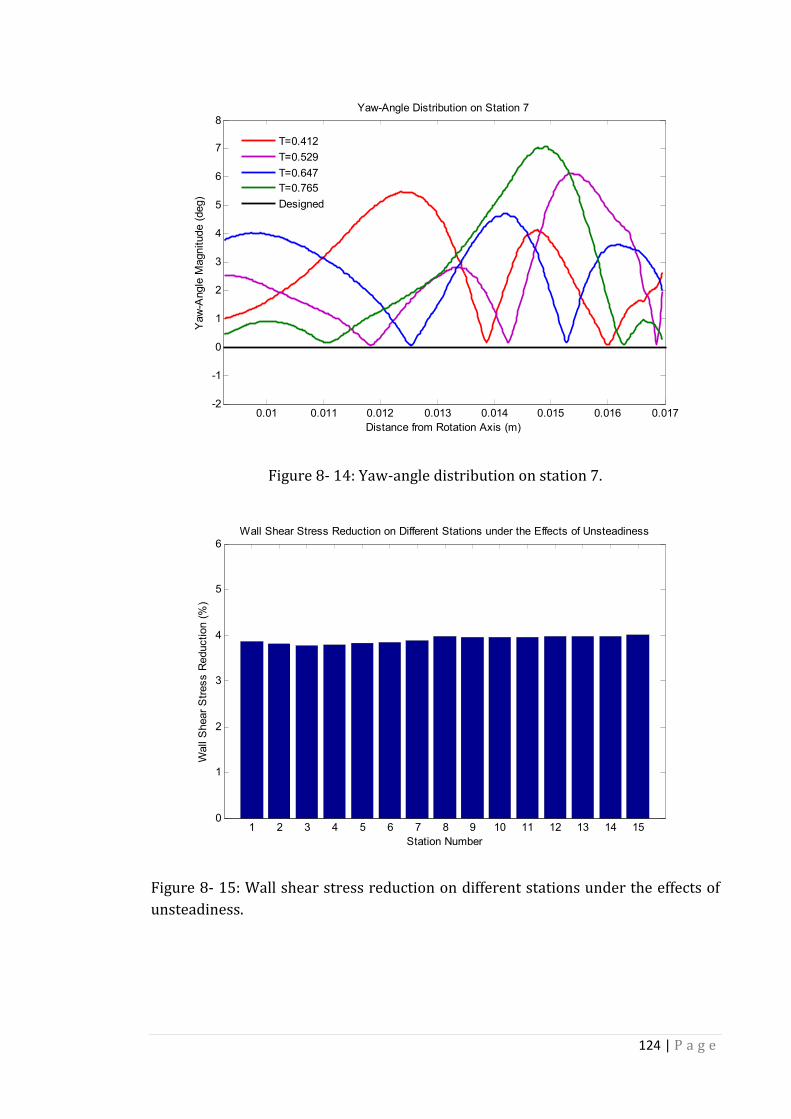
124 | P a g e
Figure 8- 14: Yaw-angle distribution on station 7.
Figure 8- 15: Wall shear stress reduction on different stations under the effects of
unsteadiness.
0.01 0.011 0.012 0.013 0.014 0.015 0.016 0.017-2
-1
0
1
2
3
4
5
6
7
8
Distance from Rotation Axis (m)
Yaw
-Angle
Magnitude (
deg)
Yaw-Angle Distribution on Station 7
T=0.412
T=0.529
T=0.647
T=0.765
Designed
1 2 3 4 5 6 7 8 9 10 11 12 13 14 150
1
2
3
4
5
6
Station Number
Wall
Shear
Str
ess R
eduction (
%)
Wall Shear Stress Reduction on Different Stations under the Effects of Unsteadiness

125 | P a g e
8.5. Summary
In this chapter, further discussions on riblets have been made, an explicit
expression has been obtained for sawtooth riblets through curving fitting on
available experimental data in literature, yaw-angle effect has also been taken into
account. Then riblets was proposed to be applied to help reduce the impeller
endwall loss for Dyson V2 centrifugal compressor. With the explicit expression and
the wall shear stress predicted from steady simulation, the riblets have been
designed, the spacing is around 35μm, a wall shear stress reduction about 4% could
be achieved. Later, the performance of the designed riblets was assessed using
unsteady simulation, thus the effects of unsteadiness could be considered. It was
confirmed that the designed riblets could perform very well, even under the effects
of unsteadiness (similar to real operation), a wall shear stress reduction around 4%
could be achieved. However, it should be noted that the current design is not
optimized for operation conditions other than Case 1.
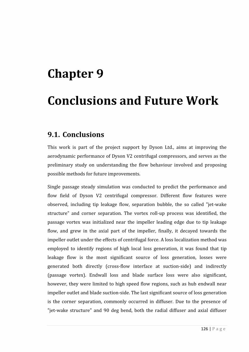
126 | P a g e
Chapter 9 Conclusions and Future Work
Conclusions and Future Work
9.1. Conclusions
This work is part of the project support by Dyson Ltd., aims at improving the
aerodynamic performance of Dyson V2 centrifugal compressors, and serves as the
preliminary study on understanding the flow behaviour involved and proposing
possible methods for future improvements.
Single passage steady simulation was conducted to predict the performance and
flow field of Dyson V2 centrifugal compressor. Different flow features were
observed, including tip leakage flow, separation bubble, the so called "jet-wake
structure" and corner separation. The vortex roll-up process was identified, the
passage vortex was initialized near the impeller leading edge due to tip leakage
flow, and grew in the axial part of the impeller, finally, it decayed towards the
impeller outlet under the effects of centrifugal force. A loss localization method was
employed to identify regions of high local loss generation, it was found that tip
leakage flow is the most significant source of loss generation, losses were
generated both directly (cross-flow interface at suction-side) and indirectly
(passage vortex). Endwall loss and blade surface loss were also significant,
however, they were limited to high speed flow regions, such as hub endwall near
impeller outlet and blade suction-side. The last significant source of loss generation
is the corner separation, commonly occurred in diffuser. Due to the presence of
"jet-wake structure" and 90 deg bend, both the radial diffuser and axial diffuser

127 | P a g e
inflow conditions were severely impacted, as a result, the diffuser stage was not
that effective in terms of pressure rise, almost 80% of the pressure rise occurred in
impeller due to strong centrifugal force. The effects of unsteadiness were also
examined using full annulus unsteady simulation, it was concluded that
unsteadiness could help reduce blockage and loss generation, and thus leads to
performance improvement.
Riblets were proposed to help reduce the impeller hub endwall loss. Although the
explicit relation between wall shear stress reduction and endwall loss is unknown,
it is sure that endwall loss will be reduced if wall shear stress is lowered. The
design was done based on flow field predicted from steady simulation, a wall shear
stress reduction about 4% could be achieved, with the optimum spacing around
35μm. Later, the effectiveness of riblets was confirmed using unsteady simulation,
even under the effects of unsteadiness, it was still possible to achieve a wall shear
stress reduction about 4%.
9.2. Future Work
Centrifugal compressor has been a very important and widely studied topic,
tremendous efforts have been expended, and the trend will continue. Only a
preliminary study has been done in this work due to the limited time (1 year).
Further studies are required to devise more methods for improving the centrifugal
compressor performance, such as:
� It has been shown that the tip leakage flow induces large amount of losses, in
small turbomachinery, it is of particular importance, although it is not possible
to be avoided, measures could be taken to weaken it. For example, the
application of vortex generator at some specific position could generate
possibly beneficial vortex, that may affect the formation path.
� In this preliminary study, the concept of applying riblets on the impeller hub
has been exploited to reduce the hub skin friction drag, and thus reduce the
associated loss generation. The explicit expression relating maximum wall
shear stress reduction to non-dimensional spacing was obtained from a single
128 | P a g e
set of data, in the future, more data can be collected to have more confidence in
the expression, different riblets configurations can also be considered.
� Tiny suction holes may be distributed at/near the leading edge of impeller
blade, and connect to slots at the base of impeller blunt trailing edge with a
plenum in between. The suction effects may help avoid the appearance of
separation bubble near the leading edge, thus reduce the loss generation (a
concept very similar to the hybrid laminar flow control technology onboard
B787). On the other hand, the jets coming out of these slots may help energize
the low momentum fluid at the base of impeller blunt trailing edge, and prompt
wake mixing, thus may help reduce the deleterious effects of wake on diffuser
performance.

129 | P a g e
Reference
Acosta, A. J. and Bowerman, R. D., 1957, "A Experimental Study of Centrifugal Pump
Impeller", Trans. of ASME, Vol. 79, pp.1821-1839.
Anderson, E. J., Macgillivray, P. S. and Demont, M. E., 1997, "Scallop Shells Exhibit
Optimization of Riblet Dimensions for Drag Reduction", Biol. Bull., Vol. 192, pp.
341-344.
Arndt, N., Acosta, A. J., Brennen, C. E. and Caughey, T. K., 1990, "Experimental
Investigation of Rotor-Stator Interactions in a Centrifugal Pump with Several Vaned
Diffusers", ASME J. Turbomach., Vol. 112, No. 1, pp. 98-108.
Bacher, E. V. and Smith, C. R., 1985, "A Combined Visualization-Anemometry Study
of Turbulent Drag Reducing Mechanisms of Triangular Micro-Groove Surface
Modification", AIAA Paper, No. 85-0548.
Bechert, D. W., Bruse, M., Hage, W., Van Der Hoeven, J. G. T. and Hoppe, G., 1997a,
"Experiments on Drag-Reducing Surfaces and Their Optimization with an
Adjustable Geometry", J. Fluid Mech., Vol. 338, pp. 59-87.
Bechert, D. W., Bruse, M., Hage, W. and Meyer, R., 1997b, "Biological Surfaces and
Their Technological Application-Laboratory and Flight Experiments on Drag
Reduction and Separation Control", AIAA Paper, No. 1997-1960.
Boese, M. and Fottner, L., 2002, "Effects of Riblets on the Loss Behavior of a Highly
Loaded Compressor Cascade", ASME Paper, No. GT-2002-30438.
Boncinelli, P., Ermini, M., Bartolacci, S. and Arnone, A., 2007, "Impeller-Diffuser
Interaction in Centrifugal Compressors: Numerical Analysis of Radiver Test Case",
AIAA J. propulsion Power, Vol. 23, No. 6, pp. 1304-1312.
CD-adapco, 2013, Star CCM+ User Guide Version 8.04.

130 | P a g e
Cebeci, T. and Carr, L. W., 1978, "A Computer Program for Calculating Laminar and
Turbulent Boundary-Layers for Two-Dimensional Time Dependent Flows", NASA
Report, No. TM 78470.
Chen, N. X., Papailiou, K. and Huang, W. G., 1999, "Numerical Study on the 3-D
Viscous Flow in a Centrifugal Compressor Impeller With and Without
Consideration of Tip Clearances", ISABE Paper, No. 99-7223.
Choi, K. S., 1989, "Near Wall Structure of Turbulent Boundary Layer with Riblets", J.
Fluid Mech., Vol. 128, No. 11, pp. 417-458.
Choi, H., Moin, P. and Kim, J., 1993, "Direct Numerical Simulation of Turbulent Flow
over Riblets", J. Fluid Mech., Vol. 255, pp. 503-539.
Clements, W. and Artt, D., 1989, "The Influence of Diffuser Vane Leading Edge
Geometry on the Performance of a Centrifugal Compressor", ASME Paper, No. 89-
GT-163.
Coustols, E., 1989, "Behaviour of Internal Manipulators: 'Riblet' Models in Subsonic
and Transonic Flows", AIAA Paper, No. 89-0963.
Dean, B. D., 2011, "The Effect of Shark Skin Inspired Riblet Geometries on Drag in
Rectangular Duct Flow", Master Thesis, The Ohio State University.
Dean, Jr., R. C. and Senoo, Y., 1960, "Rotating Wakes in Vaneless Diffusers", ASME J.
Basic Eng., Vol. 82, No. 3, pp. 563-570.
Denton, J. D., 1993, "Loss Mechanisms in Turbomachines", ASME J. Turbomach., Vol.
115, No. 4, pp. 621-656.
Dixon, S. L. and Hall, C. A., 2010, Fluid Mechanics and Thermodynamics of
Turbomachinery, 6th ed., Butterworth-Heinemann, Elsevier, USA.
Eckardt, D., 1975, "Instantaneous Measurements in the Jet-Wake Discharge Flow of
a Centrifugal Compressor Impeller", ASME J. Eng. Gas Turbines Power, Vol. 97, No. 3,
pp. 337-345.
El-Samni, O. A., Chun, H. H. and Yoon, H. S., 2007, "Drag Reduction of Turbulent
Flow over Thin Rectangular Riblets", Int. J. Eng. Sci., Vol. 45, pp. 436-454.

131 | P a g e
Enyuntin, G. V., Lashkov, Y. A. and Samoilova, N. V., 1995, "Drag Reduction in Riblet-
Lined Pipes", Fluid Dynamics, Vol. 30, No. 1, pp. 45-48.
Erdos, J. I. and Alzner, E., 1977, "Computation of Unsteady Transonic Flows
Through Rotating and Stationary Cascades", NASA Report, No. CR-2900.
Farge, T. Z., Johnson, M. W. and Maksoud, T. M. A., 1989, "Tip Leakage in a
Centrifugal Impeller", ASME J. Turbomach., Vol. 111, No. 3, pp. 244-249.
Fransson, T. H., Hillon, F. and Klein, E., 2000, "An International Electronic and
Interactive Teaching and Life-Long Learning Platform for Gas Turbine Technology
in the 21st Century", ASME Paper, No. 2000-GT-0581.
Garcia-Mayoral, R. and Jimenez, J., 2011, "Drag Reduction by Riblets", Phil. Trans. R.
Soci., Vol. 369, pp. 1412-1427.
Gottfried, D. and Fleeter, S., 2002, "Impeller Blade Unsteady Aerodynamic Response
to Vaned Diffuser Potential Fields", AIAA J. Propulsion Power, Vol. 18, No. 2, pp.
472-480.
Grek, G. R., Kozlov, V. V. and Titarenko, S. V., 1996, "An Experimental Study of the
Influence of Riblets on Transition", J. Fluid Mech., Vol. 315, pp. 31-49.
Hall, K. C., Thomas, J. P. and Clark, W. S., 2002, "Computation of Unsteady Nonlinear
Flows in Cascades Using a Harmonic Balance Technique", AIAA J., Vol. 40, No. 5, pp.
879-886.
Hathaway, M. D., Chriss, R. M., Wood, J. R. and Strazisar, A. J., 1993, "Experimental
and Computational Investigation of the NASA Low-Speed Centrifugal Compressor
Flow Field", NASA Tech. Memo., No. 4481.
Ishida, M. and Senoo, Y., 1981, "On the Pressure Losses due to the Tip Clearance of
Centrifugal Blowers", ASME J. Eng. Gas Turbines Power, Vol. 103, No. 2, pp. 271-278.
Ishida, M., Senoo, Y. and Ueki, H., 1990, "Effect of Blade Tip Configuration on Tip
Clearance Loss of a Centrifugal Impeller", ASME J. Turbomach., Vol. 112, No. 1, pp.
14-18.

132 | P a g e
Johnson, M. W. and Moore, J., 1980, "Development of Wake Flow in a Centrifugal
Impeller", ASME J. Eng. Gas Turbines Power, Vol. 102, No. 2, pp. 382-390.
Klassen, H. A., Wood, J. R. and Schumann, L. F., 1977a, "Experimental Performance
of a 16.10-Centimeter-Tip-Diameter Sweptback Centrifugal Compressor Designed
for a 6:1 Pressure Ratio", NASA Tech. , No. X-3552.
Klassen, H. A., Wood, J. R. and Schumann, L. F., 1977b, "Experimental Performance
of a 13.65-Centimeter-Tip-Diameter Tandem-Bladed Sweptback Centrifugal
Compressor Designed for a Pressure Ratio of 6", NASA Tech., No. 1091.
Koch, C. C. and Smith, L. H., 1976, "Loss Sources and Magnitudes in Axial Flow
Compressors", ASME J. Eng Gas Turbines Power, Vol. 98, No. 3, pp. 411-424.
Kolmogorov, A. N., 1942, "Equations of Turbulent Motion of an Incompressible
Fluid", Izvestia Acad. of Sci., USSR Phys., Vol. 6, No. 1, pp. 56-58.
Kozlov, V. F., Kuznetsov, V. R., Mineev, B. I. and Secundov, A. N, 1990, "The Influence
of Free Stream Turbulence and Surface Ribbing on the Characteristics of a
Transitional Boundary Layer", Proc. 1988 Zorian Zaric Mem., Near Wall Turbulence,
Hemisphere.
Krain, H., 1988, "Swirling Impeller Flow", ASEM J. Turbomach., Vol. 110, No. 1, pp.
122-128.
Launder, B. E., Reece, G. J. and Rodi, W., 1975, "Progress in the Development of a
Reynolds Stress Turbulence Closure", J. Fluid Mech., Vol. 3, pp. 269-289.
Launder, B. E. and Spalding, D. B., 1974, "The Numerical Computation of Turbulent
Flows", Comput. Methods Appl. Mech. Eng., Vol. 3, pp. 269-289.
Lietmeyer, C., Oehlert, K. and Seume, J. R., 2013, "Optimal Application of Riblets on
Compressor Blades and Their Contamination Behaviour", ASME J. Turbomach., Vol.
135, No. 1, 011036.
Lino, T. and Kasai, K., 1985, "An Analysis of Unsteady Flow Induced by Interaction
Between a Centrifugal Impeller and a Vaned Diffuser", Trans. of JSME, Vol. 51, No.
471, pp. 154-159.

133 | P a g e
Litvinenko, Y. A., Chernoray, V. G., Kozlov, V. V., Loefdahl, L., Grek, G. R. and Chun, H.
H., 2006, "The Influence of Riblets on the Development of a Λ Structure and Its
Transformation into a Turbulent Spot", Doklady Phys., Vol. 51, No. 3, pp. 144-147.
Liu, K. N., Christodoulou, C., Riccius, O. and Joseph, D. D., 1990, "Drag Reduction in
Pipes Lined with Riblets", AIAA J., Vol. 28, No. 10, pp. 1697-1698.
Liu, Z. X., Ping, Y. and Zangenen, M., 2013, "On the Nature of Tip Clearance Flow in
Subsonic Centrifugal Impellers", Sci. China Tech., Vol. 56, No. 9, pp. 2170-2177.
Mashimo, T., Watanabe, I. and Ariga, I., 1979, "Effects of Fluid Leakage on
Performance of a Centrifugal Compressor", ASME J. Eng. Gas Turbines Power, Vol.
101, No. 3, pp. 337-342.
Menter, F. R., 1992a, "Performance of Popular Turbulence Models for Attached and
Separated Adverse Pressure Gradient Flow", AIAA J., Vol. 30, No. 8, pp. 2066-2072.
Menter, F. R., 1992b, "Improved Two-Equation k-ω Turbulence Models for
Aerodynamic Flows", NASA Tech. Memo., No. TM-103975.
Menter, F. R., 1994, "Two-Equation Eddy Viscosity Turbulence Model for
Engineering Applications", AIAA J., Vol. 32, No. 8, pp. 1598-1605.
Menter, F. R., Kuntz, M. and Langtry, R., 2003, "Ten Years of Industrial Experience
with the SST Turbulence Model", Proc. 4th Int. Symp. Turbulence, Heat and Mass
Transfer, Begell House, Redding, CT.
Neumann, D. and Dinkelacker, A., 1991, "Drag Measurements on V-Grooved
Surfaces on a Body of Revolution in Axial Flow", J. Appl. Sci. Res., Vol. 48, pp. 105-
114.
Nitschke, P., 1983, "Experimental Investigation of the Turbulent Flow in Smooth
and Longitudinal Grooved Pipes", Max-Planck Ins. fur Stromungsforschung,
Gottingen.
Oehlert, K. and Seume, J. R., 2006, "Exploratory Experiments on Machined Riblets
on Compressor Blades", FEDSM Paper, No. 2006-98093.

134 | P a g e
Pampreen, R. C., 1973, "Small Turbomachinery Compressor and Fan Aerodynamics",
ASME J. Eng. Gas Turbines Power, Vol. 95, No. 3, pp. 251-256.
Peric, M., 2004, "Flow Simulation using Control Volumes of Arbitrary Polyhedral
Shape", ERCOFTAC Bulletin, No. 62.
Petit, O. and Nilsson, H., 2013, "Numerical Investigations of Unsteady Flow in a
Centrifugal Pump with a Vaned Diffuser", Int. J. Rotating Mach., Vol. 2013, ID
961580.
Plamer, D. L. and Waterman, W. F., 1995, "Design and Development of an Advanced
Two-Stage Centrifugal Compressor", ASME J. Turbomach., Vol. 117, No. 2, pp. 205-
212.
Prandtl, L., 1925, "Bericht Liber Untersungen Zur Ausgebideten Turbulenz", ZAMM,
Vol. 5, pp. 136-139.
Rai, M. M. and Madavan, N. K., 1988, "Multi-Airfoil Navier-Stokes Simulations of
Turbine Rotor-Stator Interaction", AIAA Paper, No. 88-0361.
Reynolds, O., 1901, Papers on Mechanical and Physical Subjects, Vol. 2, Forgotten
Books.
Richardson, L., 1922, Weather Prediction by Numerical Process, Cambridge
University Press, Cambridge.
Rodgers, C., 1982, "The Performance of Centrifugal Compressor Channel Diffusers",
ASME 27th Int. Gas Turbine Conf. Ex., London, England.
Rodi, W., 1980, Turbulence Models and Their Application in Hydraulics-A State of the
Art Review, IAHR, Delft, The Netherlands.
Schlichting, H., 1966, Boundary Layer Theory, 6th ed., McGraw-Hill, New York.
Schleer, M., Song, S. J. and Abhari, R. S., 2008, "Clearance Effects on the Onset of
Instability in a Centrifugal Compressor", ASME J. Turbomach., Vol. 130, No. 3,
031002.
135 | P a g e
Sciubba, E., 1994, "Entropy Production Rates as a True Measure of Viscous and
Thermal Losses in Thermodynamical Components", NATO Heat & Mass Transfer,
Bucharest.
Senoo, Y. and Ishida, M, 1987, "Deterioration of Compressor Performance due to
Tip Clearance of Centrifugal Impellers", ASME J. Turbomach., Vol. 109, No. 1, pp. 55-
61.
Shapiro, A. H., 1953, The Dynamics and Thermodynamics of Compressible Fluid Flow,
Wiley, New York.
Shum, Y. K. P., Tan, C. S. and Cumpsty, N. A., 2000, "Impeller-Diffuser Interaction in a
Centrifugal Compressor", ASME J. Turbomach., Vol. 122, No. 4, pp. 777-786.
Spalart, P. R. and Allmaras, S. R., 1992, "A One-Equation Turbulence Model for
Aerodynamic Flows", AIAA Paper, No. 92-0439.
Storer, J. A., 1991, "Tip Clearance Flow in Axial Compressors", PhD Thesis,
Cambridge University, United Kingdom.
Sundaram, S., Viswanath, P. R. and Rudrakumar, S., 1996, "Viscous Drag Reduction
Using Riblets on NACA 0012 Airfoil to Moderate Incidence", AIAA J., Vol. 34, No. 4,
pp. 676-682.
Sundaram, S., Viswanath, P. R. and Subaschandar, N., 1999, "Viscous Drag Reduction
Using Riblets on a Swept Wing", AIAA J., Vol. 37, No. 7, pp. 851-856.
Syed, D. N., Ma, C. C. and Yang, C., 2006, "Numerical Investigation of Tip Clearance
Effect on the Stage of a Tamdem-Bladed Centrifugal Compressor for Turbocharger
Application", WSEAS Trans. Fluid Mech., Vol.1, No. 6, pp. 720-725.
Tomita, I., Ibaraki, S., Furukawa, M. and Yamada, K., 2013, "The Effect of Tip
Leakage Vortex for Operating Range Enhancement of Centrifugal Compressor",
ASME J. Turbomach., Vol. 135, No. 5, 051020.
Ubaldi, M., Zunino, P., Barigozzi, G. and Cattanei, A., 1996, "An Experimental
Investigation of Stator Induced Unsteadiness on Centrifugal Impeller Outflow",
ASME J. Turbomach., Vol. 118, No. 1, pp. 41-51.
136 | P a g e
Walsh, M. J., 1980, "Drag Characteristics of V Groove and Transverse Curvature
Riblets", AIAA Progress in Astro. and Aero., Vol. 72, edited by R. G. Hough, New York,
pp. 168-184.
Walsh, M. J., 1982, "Turbulent Boundary Layer Drag Reduction Using Riblets", AIAA
Paper, No. 82-0169.
Walsh, M. J., 1983, " Riblets as a Viscous Drag Reduction Technique", AIAA J., Vol. 21,
No. 4, pp. 485-486.
Walsh, M. J. and Lindemann, A. M., 1984, "Optimization and Application of Riblets
for Turbulent Drag Reduction", AIAA Paper, No. 84-0347.
Walsh, M. J. and Weinstein, L. M., 1978, "Drag and Heat Transfer on Surfaces with
Small Longitudinal Fins", AIAA Paper, No. 78-1161.
Wang, S. L., Shi, X. J., Liu, D. and Sun, Q., 2008, "Application Studying of PIV on
Groove Drag Reduction Characteristics", ICEM 2008, edited by X. Y. He, H. M. Xie
and Y. L. Kang, Proc. of SPIE, Vol. 7375, 737520.
Wilcox, D. C., 1988, "Reassessment of the Scale-Determining Equation for Advanced
Turbulence Models", AIAA J., Vol. 26, No. 11, pp. 1299-1310.
Ziegler, K. U., Gallus, H. E. and Niehuis, R., 2003, "A Study on Impeller-Diffuser
Interaction Part I Influence on the Performance", ASME J. Turbomach., Vol. 125, No.
1, pp. 173-182.
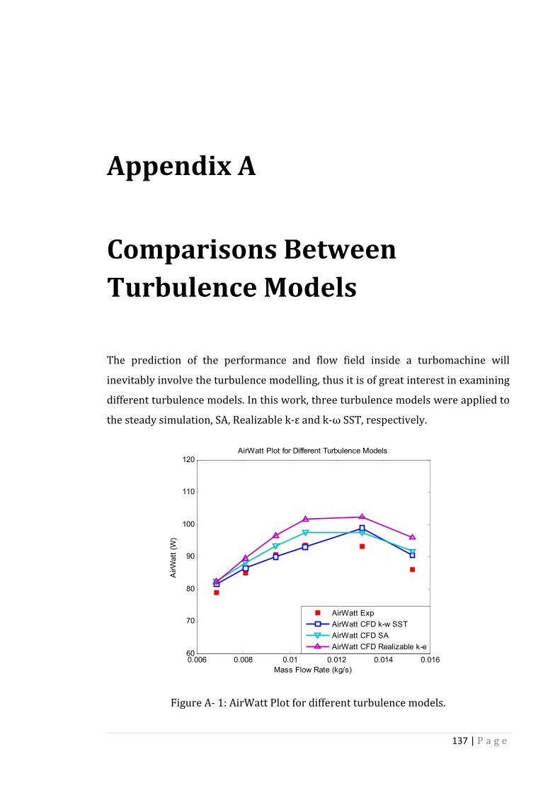
137 | P a g e
Appendix A Comparisons Between Turbulence Models
Comparisons Between
Turbulence Models
The prediction of the performance and flow field inside a turbomachine will
inevitably involve the turbulence modelling, thus it is of great interest in examining
different turbulence models. In this work, three turbulence models were applied to
the steady simulation, SA, Realizable k-ε and k-ω SST, respectively.
Figure A- 1: AirWatt Plot for different turbulence models.
0.006 0.008 0.01 0.012 0.014 0.01660
70
80
90
100
110
120
Mass Flow Rate (kg/s)
AirW
att
(W
)
AirWatt Plot for Different Turbulence Models
AirWatt Exp
AirWatt CFD k-w SST
AirWatt CFD SA
AirWatt CFD Realizable k-e
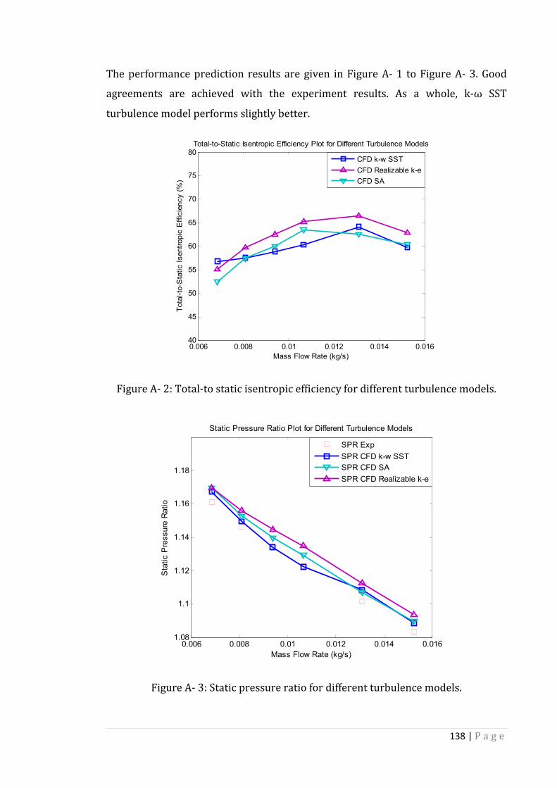
138 | P a g e
The performance prediction results are given in Figure A- 1 to Figure A- 3. Good
agreements are achieved with the experiment results. As a whole, k-ω SST
turbulence model performs slightly better.
Figure A- 2: Total-to static isentropic efficiency for different turbulence models.
Figure A- 3: Static pressure ratio for different turbulence models.
0.006 0.008 0.01 0.012 0.014 0.01640
45
50
55
60
65
70
75
80
Mass Flow Rate (kg/s)
Tota
l-to
-Sta
tic I
sentr
opic
Eff
icie
ncy (
%)
Total-to-Static Isentropic Efficiency Plot for Different Turbulence Models
CFD k-w SST
CFD Realizable k-e
CFD SA
0.006 0.008 0.01 0.012 0.014 0.0161.08
1.1
1.12
1.14
1.16
1.18
Mass Flow Rate (kg/s)
Sta
tic P
ressure
Ratio
Static Pressure Ratio Plot for Different Turbulence Models
SPR Exp
SPR CFD k-w SST
SPR CFD SA
SPR CFD Realizable k-e

139 | P a g e
Appendix B Grid Independence Study
Grid Independence Study
Grid independence study is generally required for assessing the sensitivity of the
predicted results with the grid resolution. In this work, grid independence study is
conducted for Case 1 with steady simulation. In order to obtain the fine mesh and
coarse mesh, the original mesh is doubled and halved, respectively. A summary of
the cell count is given in Table B- 1.
Cell
Count Sum
Coarse Impeller 290,000 480,000
Diffuser 190,000
Medium Impeller 530,000 900,000
Diffuser 370,000
Fine Impeller 990,000 1,640,000
Diffuser 650,000
Table B- 1: Summary of block-structured mesh.
Impeller is the primary concern of the current work, so only results related to
impeller are presented here. Figure B- 1 and Figure B- 2 present the static pressure
and wall shear stress plots at the impeller hub mid-pitch respectively, computed
with different grid resolutions, while the corresponding plots at the impeller blade
mid-span are shown in Figure B- 3 and Figure B- 4 respectively. It is observed that
the computed results are very close for different grid resolutions. Therefore, the
medium resolution grid would be adequate for the current work, and the general
flow field results in the next section are obtained with medium resolution grid.

140 | P a g e
Figure B- 1: Static pressure plot at impeller hub mid-pitch for different grid
resolutions.
Figure B- 2: Wall shear stress plot at impeller hub mid-pitch for different grid
resolutions.
0 0.005 0.01 0.015 0.02 0.025 0.03 0.0359.1
9.2
9.3
9.4
9.5
9.6
9.7
9.8
9.9
10x 10
4
Streamwise Distance (m)
Sta
tic P
ressure
(P
a)
Static Pressure Plot at Impeller Hub Mid-Pitch
Coarse
Medium
Fine
0 0.005 0.01 0.015 0.02 0.025 0.03 0.03510
20
30
40
50
60
70
80
90
100
110
Streamwise Distance (m)
Wall
Shear
Str
ess (
Pa)
Wall Shear Stress Plot at Impeller Hub Mid-Pitch
Coarse
Medium
Fine

141 | P a g e
Figure B- 3: Static pressure plot at impeller blade mid-span for different grid
resolutions.
Figure B- 4: Wall shear stress plot at impeller blade mid-span for different grid
resolutions.
0 0.005 0.01 0.015 0.028.6
8.8
9
9.2
9.4
9.6
9.8
10
10.2x 10
4
Distance from Leading Edge (m)
Sta
tic P
ressure
(P
a)
Static Pressure Plot at Impeller Blade Mid-Span
Coarse
Medium
Fine
0 0.005 0.01 0.015 0.020
50
100
150
200
250
300
350
Distance from Leading Edge (m)
Wall
Shear
Str
ess (
Pa)
Wall Shear Stress Plot at Impeller Blade Mid-Span
Coarse
Medium
Fine