numerical inverting of matrices of high …€¦ · numerical inverting of matrices of high order....
TRANSCRIPT
NUMERICAL INVERTING OF MATRICESOF HIGH ORDER. II
herman h. goldstine and john von neumann
Table of Contents
Preface. 188
Chapter VIII. Probabilistic estimates for bounds of matrices
8.1 A result of Bargmann, Montgomery and von Neumann. 188
8.2 An estimate for the length of a vector. 191
8.3 The fundamental lemma. 192
8.4 Some discrete distributions. 194
8.5 Continuation. 196
8.6 Two applications of (8.16). 198
Chapter IX. The error estimates
9.1 Reconsideration of the estimates (6.42)-(6.44) and their consequences.. 199
9.2 The general A¡. 200
9.3 Concluding evaluation. 200
Preface
In an earlier paper,1 to which the present one is a sequel, we derived
rigorous error estimates in connection with inverting matrices of
high order. In this paper we reconsider the problem from a prob-
abilistic point of view and reassess our critical estimates in this light.
Our conclusions are given in Chapter IX and are summarized in §9.3.
As in the earlier paper we have here made no effort to obtain
optimal numerical estimates. However, we do feel that within the
framework of our method our estimates give the correct orders of
magnitude.
This work has been made possible by the generous support of
the Office of Naval Research under Contract N-7-onr-388. We wish
also to acknowledge the use by us of some, as yet unpublished, re-
sults of V. Bargmann, D. Montgomery, and G. Hunt, which were
privately communicated to us.
Chapter VIII. Probabilistic estimates for bounds of matrices
8.1 A result of Bargmann, Montgomery and von Neumann. We
seek a probabilistic result on the size of the upper bound of an nth
order matrix which was first established by Bargmann, Mont-
gomery, and von Neumann. Since the result is contained in an as
yet unpublished paper, we give below an outline of the proof and also
Received by the editors February 27, 1950.
1 Numerical inverting of matrices of high order, Bull. Amer. Math. Soc. vol. 53
(1947) pp. 1021-1099. The numbering of chapters and sections in the present paper
follows directly upon those of the one just cited.
188
License or copyright restrictions may apply to redistribution; see http://www.ams.org/journal-terms-of-use

NUMERICAL INVERTING OF MATRICES OF HIGH ORDER. II 189
we modify slightly the final theorem. Let
(8.1) A = («,,) (*. j = 1. 2, • • • , n)
be a matrix whose elements are independent random variables, each
of which is normally distributed with mean zero and dispersion a.
Under these assumptions it is well known2 that
(a) The joint distribution function for the elements a,y (*', j
= 1,2, • • ■ , n) is given by
1
ff»(2r)"'*exp
2Z an
II dau;
(b) The joint distribution function for the elements of the definite
matrix A*A =5 = (Z>¿y) (t, j = i, 2, • • • , n) is given by
Wn"(bif>^f)
(Det B)-"2
(2i'v)»V"(—i>'4n r(-)1=1 \ 2 /
exp
z »«2^2 j
(c) The joint distribution function for the n proper values, Xi, X2|
• • , X„ of the matrix B is given by
Kn exp
Ex.
2o-2
where'
-ra/S
Km =
(8.2)
(2,,-n(r(-^i))
Pm/2
<W"-ñ(r(f))'(m= 1,2, •••)•
! Cf. for example, S. S. Wilks, Mathematical statistics, Princeton, 1943, pp. 226 ff"
3 Cf. S. S. Wilks, op. cit., pp. 262-263. In his results n — 1 should be replaced by
», X by a2, and U by Xi (t = l, 2, •••,») to make them consistent with our nota-
tional practices.
License or copyright restrictions may apply to redistribution; see http://www.ams.org/journal-terms-of-use

190 H. H. GOLDSTINE AND JOHN VON NEUMANN [April
Next
(8.3) Assume that X=Xi is the largest proper value of B and that
<p(X) is its probability density. Then, if r ^ 1",
/ 2r Y 1Prob (X > 2a2m) < (-IX-
Ve1-1/ 4(r - \)(nnY>2
To prove (8.3) let R be the region of (»—1)-dimensional space
X¿ = 0 (i=2, 3, ■ • • , n) and for each X>0 let R\ be the sub-region of
R consisting of all (X2, X3, ■ • • , X„) such that XïîX2Sï • • • èX„èO.
We then see that
0(X) = KJr11* exp(-^)/ÄxeXP
£x,
(8.4.a)
IT (X< - Xi) II (* - Xi-)*} d\i2ái<í j-2
^ Kn\n'il2 exp
\ 2W JÄXexp
Zh
■ n (x, - x,) n x, d\j%Si<i i=2
g XnX""3/2 exp ( - —- j f exp
2><
2<r2
n (x.- - xf) n x, d\2S«J
= \"-u2exp(--^AKnKníi;
the first inequality follows at once from the fact that X—Xy=X
(j = 2, 3, ■ ■ - , n), the second from the fact that R\ER and the last
equality is a known result.4 It now follows easily from (8.2) that
(8.4.b)Kn rl/2
Kn-i (2o-2Y-v2(Y(n/2))2
and hence summing up, we have
4 Cf. S. S. Wilks, op. cit., pp. 263-264.
License or copyright restrictions may apply to redistribution; see http://www.ams.org/journal-terms-of-use
195»] NUMERICAL INVERTING OF MATRICES OF HIGH ORDER. II 191
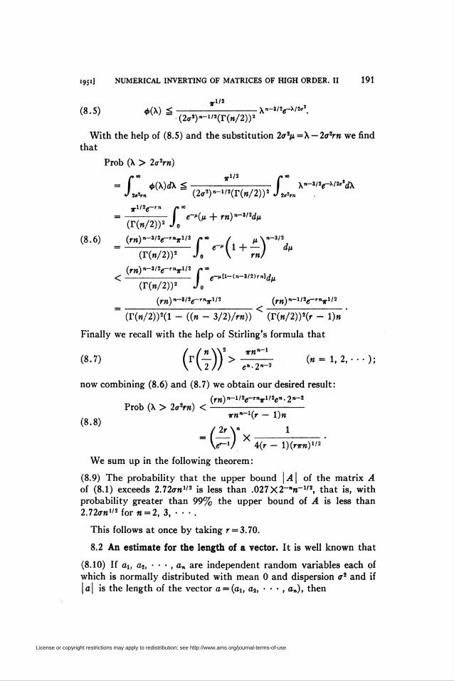
(8.5) 4>CK) <-Xn-3ne-xi2„\(2<r2)"-1/2(r(«/2))2
With the help of (8.5) and the substitution 2a2p.=\ — 2a2rn we find
that
Prob (X > 2<rVM)
*(X)áX ^- \»-*i2e-*i2°%d\2„V* - i20-2)^2iVin/2))2 J 2^rn .
Tl/2e-rn
f «-"(/* + rn) "-3'2d/nJo
e-» I 1 + — ) dp.iYin/2))2 Jo \ m
(r(«/2))2 J„
(8.6) (m)"-3/2e-r"ir1/2 ("° ( m\"~3/2
M"-3/2e---"ir1/2 Z*00
(r(«/2))!J e-?H-(.n-3l2)rn
JoUn
irny-uh-'»-*1'2 (r»)»-1'2«-'»*-1'2
(r(«/2))2(l - ((n - 3/2)/r»)) (r(«/2))2(r - 1)«
Finally we recall with the help of Stirling's formula that
/ /«NX2 x«"-1
(87) Kt/PT^ H-«.*.•■••)!now combining (8.6) and (8.7) we obtain our desired result:
(rw)n-l/2i-rn7rl/2en.2»-2
Prob (X > 2tr2r«) <-irwn_1(r — l)w
(8-8) ..... j
X-£)"4(r - lXrx»)1'*
We sum up in the following theorem:
(8.9) The probability that the upper bound | A | of the matrix A
of (8.1) exceeds 2.72o-«1'2 is less than .027X2-"w-1/2, that is, with
probability greater than 99% the upper bound of A is less than
2.720-w1'2 for n = 2, 3, • • • .
This follows at once by taking r = 3.70.
8.2 An estimate for the length of a vector. It is well known that
(8.10) If ax, a2, ■ ■ • , an are independent random variables each of
which is normally distributed with mean 0 and dispersion a2 and if
\a\ is the length of the vector a = (oi, a2, ■ ■ • , a„), then
License or copyright restrictions may apply to redistribution; see http://www.ams.org/journal-terms-of-use

192 H. H. GOLDSTINE AND JOHN VON NEUMANN [April
(8.11) P(\a\ > (a2™)1'2) = - f x'-W2*2^.611 2»'V»r(«/2) J c,w'2
Let n = 2N and y=x2; then (8.11) becomes
P(\a\ < (2o-2rNyi2) =- f y"-le-*i**dy.11 2^r2*r(A0J2,'rl/
Since the integral on the right is of the same form as the one in (8.6),
we see by the same sort of argument which led to (8.8) that
, i (rN)NP(\a\ > (2o-2rN)1'2) <
erNN(r - l)T(N)
/ r Y 1<(-) X->
\e-V tt1'2^ - 1)(2A0"2
that is, we have
(8.12) For random vectors a, as defined in (8.10), we have
(8.13.a) P(\ a\ > „(rn)"2) < (re1-)"'2 X -——-—>(vn)ll2(r — 1)
(8.13.b) P(\ a\ > 1.92(rw1/2) < 0.21 X 2~".
The last inequality follows at once from (8.13.a) by setting
r = 3.70.
8.3 The fundamental lemma. To describe the result upon which
the body of the paper depends we need two definitions.
(8.14) Designate by Ui(a) the Ith convolution of the uniform distri-
bution on the interval —a, +ct.
(8.15) Let 0 be a non-negative valued function defined on a real
Af-dimensional euclidean space and let it have the properties:
(a) <f> is continuous and convex, that is, for aj^b, <p((a + b)/2)
ú(<p(a)+<b(b))/2.(b) <p is positively homogeneous, that is, <p(sa) = \s\ -<i>(à) for
every real number 5.
(c) <f> has bound 1, that is if |a| ^1, $(a) = l.
If M = n2 and if the point o = («i, a2, • • • , ajif) is interpreted as an
wth order matrix, then the bound satisfies the properties (a)-(c) of
(8.15). Similarly, if M = » and if a is interpreted as a vector, then the
6 Cf. for example, Cramer, Mathematical methods of statistics, Princeton, 1946, p.
236.
License or copyright restrictions may apply to redistribution; see http://www.ams.org/journal-terms-of-use
'95'1 NUMERICAL INVERTING OF MATRICES OF HIGH ORDER. II 193
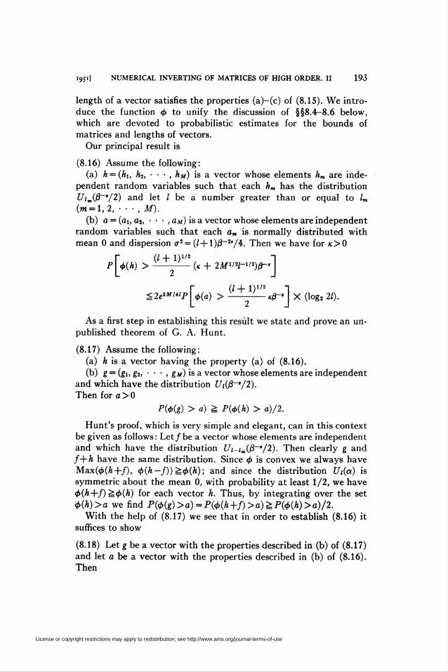
length of a vector satisfies the properties (a)-(c) of (8.15). We intro-
duce the function <f> to unify the discussion of §§8.4-8.6 below,
which are devoted to probabilistic estimates for the bounds of
matrices and lengths of vectors.
Our principal result is
(8.16) Assume the following:
(a) h = ihi, h2, ■ ■ • , h)t) is a vector whose elements hm are inde-
pendent random variables such that each hm has the distribution
Uimiß~'/2) and let I be a number greater than or equal to lm
(«-1,2, • ■ -, M).(b) a = (ai, a2, ■ ■ ■ , auf) is a vector whose elements are independent
random variables such that each am is normally distributed with
mean 0 and dispersion <r2 = (/+l)/3~2''/4. Then we have for k>0
r (/+i)i/2 iP\ <t>ih) > --— (k + 2M1'2/-1'2)jr'
r (¿ + i)i/2 i^2e*Ml*'P\ 4>ia) >-— «0- X (logi 21).
As a first step in establishing this result we state and prove an un-
published theorem of G. A. Hunt.
(8.17) Assume the following:
(a) h is a vector having the property (a) of (8.16).
(b) g = igi, g2, ■ ■ ■ , gin) is a vector whose elements are independent
and which have the distribution Uiiß~'/2).
Then for a > 0
Pitig) > m) à Piïih) > a)/2.
Hunt's proof, which is very simple and elegant, can in this context
be given as follows: Let /be a vector whose elements are independent
and which have the distribution Ui-imiß~'/2). Then clearly g and
f+h have the same distribution. Since <b is convex we always have
Max(<£(A+/), (pih—f))^<pih); and since the distribution U¡ia) is
symmetric about the mean 0, with probability at least 1/2, we have
<t>ih+f) =<)>ih) for each vector h. Thus, by integrating over the set
4»(h)>a we find P(^(g)>o)=P(^(A+/)>o)èP(*(*)>o)/2.
With the help of (8.17) we see that in order to establish (8.16) it
suffices to show
(8.18) Let g be a vector with the properties described in (b) of (8.17)
and let a be a vector with the properties described in (b) of (8.16).
Then
License or copyright restrictions may apply to redistribution; see http://www.ams.org/journal-terms-of-use
194 H. H. GOLDSTINE AND JOHN VON NEUMANN (April
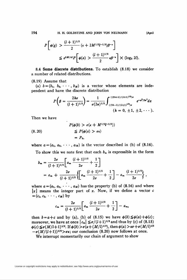
r (¿ + 1)1/2 1P <t>(g) > -(« + 2M1'H-1i2)ß-'
r (/+i)i/2 ig e^inp 0(a) > :-Kßr. x (jog2 21).
8.4 Some discrete distributions. To establish (8.18) we consider
a number of related distributions.
(8.19) Assume that
(a) b = (bi, b2, ■ ■ • , ¿»m) is a vector whose elements are inde-
pendent and have the discrete distribution
/ 2hc \ 1 /.<(2A+i)/a+i)"2),P ( ß = -) =- I e-*2l2°zdx
\ (l+iy2/ (^»^J^d/c+dI/V
(A = 0, ±1, ±2, •••)•
Then we have
P(4>(b) > c(k + M1'2/"1'2))
(8.20) g P(<p(a) > ac)
= Po,
where a = (ci, a2, • • • , ait) is the vector described in (b) of (8.16).
To show this we note first that each bm is expressible in the form
2<r f (/ + l)1'2Ôm =
(/+1)
= am +
r (i+iy2 in
^r-2^~ + TJa ¡r (i +1)1'2 in (i + i)»'n
ipT,tLa"-i7-+¥j-a--ir-ia+Dwhere a = (oi, a2, • • • , oaî) has the property (b) of (8.16) and where
[x] means the integer part of x. Now, if we define a vector c
= (fti c2, • • • , caí) by
2ff r (J + i)i/2. i
(*+D
r (/ + i)"2 i -i
i'2 L 2<r 2 J
then 6 = a+c and by (a), (b) of (8.15) we have <b(b) <<b(a)+<i>(c);
moreover, we have at once | cm\ áo-/(/+l)1/2 and thus by (c) of (8.15)
<j>(c)èa(M/l+\yi2.li<t>(b)>o-(K+(M/iyi2),then<t>(a)>K<j+a(M/iyi2
— ff(M/(l+í))ll2>aK; our conclusion (8.20) now follows at once.
We interrupt momentarily our chain of argument to show
License or copyright restrictions may apply to redistribution; see http://www.ams.org/journal-terms-of-use
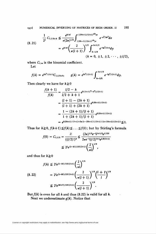
1951] NUMERICALINVERTINGOFMATRICESOFHIGHORDER.il 195
J C3/4I /. ((2A+1)/<î+1)W)ï
(8.21)
= e3/4¡
/. UZA+1)/
/ 2 V'2 fh+m
\t(Z+1)/ Ja_1/2
(A = 0, ±1, ±2, ••• , ±1/2),
where Ci,m is the binomial coefficient.
Let
/• Ä+l/2 e-tfl('+»dyh-llî
Then clearly we have for h ̂ 0
/(A + 1) //2 - h
fih) 1/2 +h+i
(/+!)- (2A + 1)
e2((/.+l)2-*i)/((+l)
(/ + 1) + (2Ä + 1)
1 - (2A + !)/(/ + 1)
C2(2A+1)/(I+1)
e2(2Ä+l)/(!+l)
1 + (2Â + 1)/(Z + 1)
= e2(2A+l)/(i+l)+ln(l-(2A+l))/(l+l)/(l+(2A+l)/(l+l))^ J_
Thus for AèO, /(A+l) S/(A)á. ■ ■ 3/(0); but by Stirling's formula
Í! (27r)1'2e-i/!+1'2e1/12i
/(O) = C,.i„ = ——— ^((//2)!)2 27re-!(//2)i+V"('+1>
/2\1'2< 2!c<1-3í>'12í(¡+1>|_)
VW 'and thus for A 3:0
1/2
/(A) ^ 2ie(1-3!)/12i(!+1)( —)
2
ifj+l),
< 2ig(»I+7)/12I(I+l)( - \
\ir(i+l)/
/ 2 V'2// + IX1'2(8.22) = 2'e<1-3i)'12!(!+1)(-) (-)
\t(/+1)/ \ / /
But/(A) is even for all A and thus (8.22) is valid for all A.
Next we underestimate g(A). Notice that
License or copyright restrictions may apply to redistribution; see http://www.ams.org/journal-terms-of-use
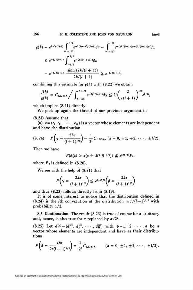
196 H. H. GOLDSTINE AND JOHN VON NEUMANN [April
/1/2 /.1/2e-2(A+x)2/(¡+l)¿£ _ g-(4A/(!+l))i-(2/(¡+l))j:2¿;r
-1/2 J-112
I'i 1/2
> g-l/2(í+l) I e-{ihW+l))x¿x
'-1/2
sinh (2h/(l + 1))= g-l/2(!+l) _i_Li_!_ÍL > g-I/2(i+l).
2h/(l + 1)
combining this estimate for g(h) with (8.22) we obtain
fW / f"+1/2 . / 2 V'2
which implies (8.21) directly.
We pick up again the thread of our previous argument in
(8.23) Assume that
(a) c = (ci, c2, ■ • ■ , cm) is a vector whose elements are independent
and have the distribution
±1/2)./ 2ha \ 1
(8-24) PV = J+~îyT2)= rCu,2+h {h = 0, ±1, +2, '
Then we have
P(<b(c) > o-(k + M'lH-V2)) Ú «3M/4!Po,
where P0 is defined in (8.20).
We see with the help of (8.21) that
/ 2h<r \ / 2hc \P[y =-I < e*'ilP[ß = -)
V (/+1)1'2/" V (/+1)1/2/
and thus (8.23) follows directly from (8.19).
It is of some interest to notice that the distribution defined in
(8.24) is the Ith convolution of the distribution +o-/(/-|-l)1/2 with
probability 1/2.
8.5 Continuation. The result (8.23) is true of course for a arbitrary
and, hence, is also true for a replaced by <r/2p.
(8.25) Let d^ = (d(?\ d2p), ■ ■ ■ , a*?') with p = l, 2, ■ ■ ■ , q be avector whose elements are independent and have as their distribu-
tions
p(8 = 2Kik+\y>) = ^Cl-m+h (* "0| ±1, ±2, ' ' " ' ±l/2)-
License or copyright restrictions may apply to redistribution; see http://www.ams.org/journal-terms-of-use
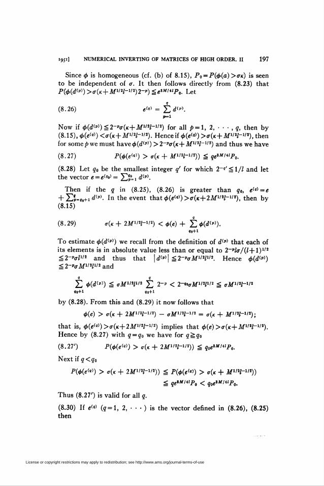
1951] NUMERICAL INVERTING OF MATRICES OF HIGH ORDER. II 197
Since <p is homogeneous (cf. (b) of 8.15), Po = P(0(a) ><r/c) is seen
to be independent of <r. It then follows directly from (8.23) that
P(<Há(!,)) ><r(/c+M1/2/-1'2)2-") ^e3MlilPo. Let
(8.26) «<«> = ¿d<»>.
Now if <pid^)^2-"o-ÍK + M1'n-1i2) for all p = \, 2, ■ ■ ■ , q, then by
(8.15),<^.(e<'))<^(«+^1/^1/2). Hence if <¿>(e(,)) ><t(k+M "W), then
for some^we must have<¿>(¿(í>)) >2_po-(k-(-M1/!!/_1/2) and thus we have
(8.27) P(<He(,)) > *(* + M1'2/-1'2)) g qe*MiilP0.
(8.28) Let go be the smallest integer q' for which 2~?'gl/7 and let
the vector e = e<«o> = ^°=1 d<«>>.
Then if the g in (8.25), (8.26) is greater than q0, e<«>=e
+ Zl=í0+i¿(p)- In the event that0(e<«))>o-(K+2M1'2/-1/2), then by
(8.15)
(8.29) o-Ík + 2M1'2/-1'2) < <t>ie) + ¿ 0(¿(p)).«o+l
To estimate <£(d(p)) we recall from the definition of ¿(p) that each of
its elements is in absolute value less than or equal to 2~"lo-/il+l)112
á2-%¿1'í and thus that |d«| ^-"o-M1'2/1'2. Hence 0(¿(p))
^2-"o-M1'2/1'2and
¿ <¿>(¿<p>) g o-M^H1'2 ¿ 2-p < 2-«o<rM1'2"'2 ^ crM1'2/-1'2
«o+l «o+l
by (8.28). From this and (8.29) it now follows that
<j>ie) > o-Ík + 2M1'2/-1'2) - o-M^H-1'2 = <r((c + M1'2/-»'2);
that is, <^)(e<«))>o-(K-(-2Af1'2/-1/2) implies that 0(e) >o-(/c+M1/2Z-1/2).
Hence by (8.27) with q = qo we have for q^qo
(8.27') PO(«(l)) > <r(/c + 2M1iH-1'2)) £ ?0e8Af/4iPo.
Next if g < go
P(tf>(e(s)) > «r(ic + 2M1'2/-1'2)) è P(<Ke(4)) > cr(K + M1'2/"1'2))
g qeiMlilPo < qoeiM'ilP0.
Thus (8.27') is valid for all q.
(8.30) If e<«> {¡mi, 2, ■ ■ ■ ) is the vector defined in (8.26), (8.25)then
License or copyright restrictions may apply to redistribution; see http://www.ams.org/journal-terms-of-use
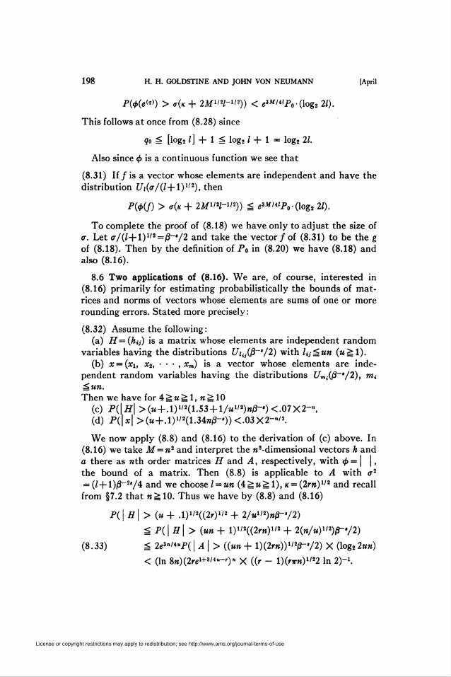
198 H. H. GOLDSTINE AND JOHN VON NEUMANN [April
P(<t>(eW) > o-(k + 2M"2l~v2)) < eiM'ilPo-(\o%2 21).
This follows at once from (8.28) since
ço è [log2 /] + 1 á log21 + 1 - log2 21.
Also since <p is a continuous function we see that
(8.31) If / is a vector whose elements are independent and have the
distribution Ui(<r/(l+l)112), then
P(4>(f) > "(k + 2M1'2/"1'2)) è e3W/4îPo-(log2 21).
To complete the proof of (8.18) we have only to adjust the size of
a. Let o-/(l+\yt2 = ß~'/2 and take the vector / of (8.31) to be the g
of (8.18). Then by the definition of P0 in (8.20) we have (8.18) and
also (8.16).
8.6 Two applications of (8.16). We are, of course, interested in
(8.16) primarily for estimating probabilistically the bounds of mat-
rices and norms of vectors whose elements are sums of one or more
rounding errors. Stated more precisely:
(8.32) Assume the following:
(a) H=(hij) is a matrix whose elements are independent random
variables having the distributions Uiij(ß~"/2) with Uj^un (m^I).
(b) x = (xi, x2, • • • , xm) is a vector whose elements are inde-
pendent random variables having the distributions Umi(ß~'/2), mt
^un.
Then we have for 4 à w â 1, « è 10
(c) P(|77| >(M-r-.l)1/2(1.53 + l/M1/2)«/3-')<.07X2-",
(d) P(\x\ >(u+.iyi2(iMnß-'))<.03X2-n'2.
We now apply (8.8) and (8.16) to the derivation of (c) above. In
(8.16) we take M = n2 and interpret the w2-dimensional vectors A and
a there as «th order matrices 77 and A, respectively, with <j>=\ \ ,
the bound of a matrix. Then (8.8) is applicable to A with a2
= (l + l)ß-~2,/4: and we choose l = un (4èw^l), K = (2rn)112 and recall
from §7.2 that n^ 10. Thus we have by (8.8) and (8.16)
P( | H | > (u + .iy>2((2ryi2 + 2/u"2)nß-/2)
g P( | 77 | > (un + iyi2((2my'2 + 2(n/uy2)ß-'/2)
(8.33) g 2e3n'4"P( \A\> ((un + l)(2rn)yi2ß~'/2) X (log2 2««)
< (In 8»)(2re1+3/4«-'')" X ((r - í)(rrn)li22 In 2)"1.
License or copyright restrictions may apply to redistribution; see http://www.ams.org/journal-terms-of-use

1951] NUMERICAL INVERTING OF MATRICES OF HIGH ORDER. II 199
To complete the argument we note that u è 1 and take r = 4.7. Then
2^1+3/4-^1/2 and for we 10, (In %n)/n"2^i\n 80V101'2.
We next apply (8.13.a) and (8.16) to the derivation of (d) above.
In (8.16) we, this time, take M = n and <f> to be the length of a vector.
Then (8.13.a) is applicable to the vector a with <r2=(/+l)/S-2s/4
and we choose l = un, k = (r»)1/2. Thus, we have by (8.13.a.) and (8.16)
Pi | x | > (w +.l)»/»((m)1" + 2/u1>2)n1i2ß-/2)
g P(| x\ > iun + l)1'2«™)1'2 + 2/ul'2)ß~'/2)
è 2e3'4«P( | a | > Hun + \)mY'2 ß~'/2 X (log2 2m»)
< (2 In ^e^'ire^Y^-Hr - lX«*)*" In 2)"1
(In 8«)= 2e3'4- irel-r)»'2iir - l)*1'2 In 2)"1.
«1/2
To complete the argument we take r = 4 and note that (« + .1)1/2
X (1.34«) è(M+.l)1/2(n1/2+l/M1'2)n1'2 for »^10.
Chapter IX. The error estimates
9.1 Reconsideration of the estimates (6.42)-(6.44) and their con-
sequences. The decisive estimates of §§6.3-6.10 are (6.42), (6.43), and
(6.44) and they yield (6.96) and (6.102) almost directly. We proceed
now to replace the strict estimates (6.42)-(6.44) by probabilistic
ones. These replacements are all based upon (8.32) ; and since we
assume «^10 they have probabilities of at least 99.9%.
First, we apply (8.32) to the matrix of (6.33) and see by (6.29)
that the u of (8.32) can be taken to be 2. Thus with high probabilitywe can replace (6.34) and the equivalent (6.42) by
(9.1) \2 - B*DB\ ú 3.25nß~'.
Second, we apply (8.32) to the matrix U of (6.39) and see by (6.39)
that m can be taken to be 4. Thus we replace (6.43) by
(9.2) \ U\ Ú 4.12«j3-'.
Third, we apply (8.32) to the vectors Um and see by (6.39) that
u can be taken to be 4. Thus we replace (6.44) by
(9.3) | i/m| ^ 2.72M/3-.
Next we define
(9.4) a' = 8nß-'/ti,
License or copyright restrictions may apply to redistribution; see http://www.ams.org/journal-terms-of-use
200 H. H. GOLDSTINE AND JOHN VON NEUMANN [April
and notice that (9.2)-(9.4) imply
(9.5) I J- WOB] < A2ß<x',
(9.6) I U\ < .58/x«',
(9.7) | i/m | g .34*«*'.
Thus (9.5)-(9.7) are in form the same as (6.42)-(6.44) except that a
has been replaced by a'.
The estimate (6.65") will now be valid with a replaced by a',
provided only that (6.62) and (6.67) are valid under this same re-
placement. Using (8.32) with m = 4, we find that (6.56) becomes
(9.9) | W^ - 2-"ZA-2D-iZ* | ^ 4.12w/3-J < .91Ma'.
If now we assume that
(9.10) a' Ú -1,
then we have
(9.11) | 2q"Ä.Wo - 7| < (1.98 + 10.28XV,
where q0 is defined in (6.59).
9.2 The general AT. By analogy with (6.73) and (9.4) we define
(9.12) ai = %nß~'/ ¿.
Then with the help of (8.32) with »=1 we can replace (6.75) by
(9.13) | J - Ail* | < 2.66nß~' < ßla'i/2,
and thus (6.78') and (9.10) can be replaced by
ai ^ .095.
All the results of §§6.9-6.11 are now valid with a¡ replaced by a\
and in particular (6.102) is now
(9.14) | 2ixAiS - 71 g (5.29 + 14.55Xí)<*z,
where Ci is defined by (6.92).
9.3 Concluding evaluation. In closing it is desirable for us to
evaluate once again our conclusions in a final capitulation.
First, the requirements of §§7.2 and 7.3 are unchanged except for
(7.2), (7.2/) which are now
(9.15) a' S .1, that is /x è &0nß-',
(9.15r) ai è .095, that is /»r ̂ 84.2w/T\
License or copyright restrictions may apply to redistribution; see http://www.ams.org/journal-terms-of-use

1951] NUMERICAL INVERTING OF MATRICES OF HIGH ORDER. II 201
Second in the light of (9.11), (9.14), (7.5'), (7.5'/) now become
(9.16) I 23lWo - l\ á 114(X/M)«/3-\
(9.16/) I 2îlJz5 - l\ S 293(X//V/)«/T\
and the conditions which are the negations of (9.15), (9.15/) are
(9.17) m < 80nß~\
(9.17/) mi < 84.2»/3-s.
Thus we have either (9.16) or (9.17) for J and either (9.16/) or (9.17/)
for J/. The conditions (9.16), (9.16/) express that 2q«Wo and 2«i£ are
approximate inverses for A and Ar, respectively, while the conditions
(9.17), (9.17/) express that A and Ar, respectively, are approximately
singular.
It is perhaps worth remarking that the coefficients 114 and 293
appearing in (9.16), (9.16/) and the coefficients 80, 84.2 in (9.15),
(9.15/) are probably not optimal, but result from the crudeness of
our probabilistic techniques. However, our principal aim was not to
produce "best possible" estimates, but was merely to obtain a feeling
for the sizes of the errors likely to be encountered.
By analogy with §7.8 we conclude with some numerical evaluations
of our estimates (9.16), (9.17) for J and (9.16/), (9.17/) for 1/. Let
us accept the probabilistic estimates (7.14/.a)-(7.14/.c) for X/, nr and
(7.14'.a)-(7.14'.c) for X, n. Then (9.17), (9.17/) imply approximately
(9.18) n ^ .01/3"2;
that is, an approximate inverse will usually be found if
(9.18') n < .0l3"2.
Furthermore, the right-hand sides of the estimates (9.16), (9.16/)
become (again approximately)
(9.19) ^ 20,000»3/3-«.
(In the case of (9.16) the factor 20,000 should have been ~11,000
and in the case of (9.16/) <~29,000. Cf. the remarks immediately
succeeding (7.16); the remarks made there are substantially ap-
plicable here.)
For this to be less than one, we have
(9.18") n < (/3'/20)1'3/10 < .04/3"3;
that is, an approximate inverse will usually be found if n satisfies the
condition (9.18"). If we assume that 0*^1O4, which is certainly
License or copyright restrictions may apply to redistribution; see http://www.ams.org/journal-terms-of-use

202 W. H. SPRAGENS [April
reasonable, then condition (9.18") is more stringent than (9.18')
and we therefore regard it as the critical condition regarding the rela-
tive precision of the approximate inverse.
Considering the precisions (7.17.a)-(17.17c), we find that (9.18")
becomes
(9.19.a) n < 19,
(9.19.b) n < 86,
(9.19.c) «<400.
Institute for Advanced Study
ON SERIES OF WALSH EIGENFUNCTIONS
W. H. SPRAGENS
Walsh [4]1 considered expansions in terms of eigenfunctions satis-
fying the equation
u"(x) + [p2 - g(x)]u(x) = 0, OS irai,
and the boundary conditions
«(0) = 0, «(1) = 0,
the function g(x) being assumed continuous on Ogxgl. He used the
asymptotic formula for the £th eigenfunction
(1) **(*) = (2)1'2[sin kirx + (\/k)$k(x)}, I <l>k(x) I è C.
Comparing series of these functions with corresponding series of
the functions
(2) uk(x) = (2)1'2 sin krx,
he proved that if a function in L2 is expanded in terms of both sets of
functions, then the series of term-by-term differences converges uni-
formly and absolutely to zero on O^xéí.
This result, as Walsh points out, is closely related to that of Haar
[l], who considered the Sturm-Liouville problem with boundary
conditions u'+Hu = 0, and compared the series of the resulting func-
tions with the Fourier cosine series. He obtained equiconvergence in
Received by the editors April 3, 1950.
1 Numbers in brackets refer to the references cited at the end of the paper.
License or copyright restrictions may apply to redistribution; see http://www.ams.org/journal-terms-of-use