nuisance hardened data compression for fast likelihood

MNRAS 000, 1–12 (2018) Preprint 6 March 2019 Compiled using MNRAS LATEX style file v3.0

Nuisance hardened data compression for fastlikelihood-free inference

Justin Alsing1,2,3? and Benjamin Wandelt2,41Oskar Klein Centre for Cosmoparticle Physics, Stockholm University, Stockholm SE-106 91, Sweden2Center for Computational Astrophysics, Flatiron Institute, 162 5th Ave, New York City, NY 10010, USA3Imperial Centre for Inference and Cosmology, Department of Physics, Imperial College London, Blackett Laboratory,Prince Consort Road, London SW7 2AZ, UK4Sorbonne Universite, Institut Lagrange de Paris (ILP), 98 bis boulevard Arago, F-75014 Paris, France

Accepted XXX. Received YYY; in original form ZZZ

ABSTRACTIn this paper we show how nuisance parameter marginalized posteriors can be inferreddirectly from simulations in a likelihood-free setting, without having to jointly infer thehigher-dimensional interesting and nuisance parameter posterior first and marginalizea posteriori. The result is that for an inference task with a given number of interestingparameters, the number of simulations required to perform likelihood-free inferencecan be kept (roughly) the same irrespective of the number of additional nuisancesto be marginalized over. To achieve this we introduce two extensions to the stan-dard likelihood-free inference set-up. Firstly we show how nuisance parameters can bere-cast as latent variables and hence automatically marginalized over in the likelihood-free framework. Secondly, we derive an asymptotically optimal compression from Ndata down to n summaries – one per interesting parameter – such that the Fisher in-formation is (asymptotically) preserved, but the summaries are insensitive (to leadingorder) to the nuisance parameters. This means that the nuisance marginalized infer-ence task involves learning n interesting parameters from n “nuisance hardened” datasummaries, regardless of the presence or number of additional nuisance parameters tobe marginalized over. We validate our approach on two examples from cosmology: su-pernovae and weak lensing data analyses with nuisance parameterized systematics. Forthe supernova problem, high-fidelity posterior inference of Ωm and w0 (marginalizedover systematics) can be obtained from just a few hundred data simulations. For theweak lensing problem, six cosmological parameters can be inferred from just O(103)simulations, irrespective of whether ten additional nuisance parameters are includedin the problem or not. If needed, an approximate posterior for the nuisance parame-ters can be re-constructed a posteriori as a pseudo-Blackwell-Rao estimator (withoutrunning any additional simulations).

Key words: data analysis: methods

1 INTRODUCTION

Likelihood-free inference is emerging as a new paradigmfor performing principled inference from cosmological datausing forward simulations only, incorporating exactly allknown effects that can be successfully simulated without re-lying on approximate likelihoods (Schafer & Freeman 2012;Cameron & Pettitt 2012; Weyant et al. 2013; Robin et al.2014; Lin & Kilbinger 2015; Ishida et al. 2015; Akeret et al.2015; Jennings et al. 2016; Hahn et al. 2017; Kacprzak et al.

? E-mail: [email protected]

2017; Carassou et al. 2017; Davies et al. 2017; Alsing et al.2018b, 2019).

In Alsing et al. (2018b, 2019) we showed that likelihood-free inference is achievable from just O(103) forward simu-lations for typical problems in cosmology, with n ∼ 6 or socosmological parameters of interest. However, while manyproblems have a small number of interesting parameters,they often come with a large number of additional nuisanceparameters that ultimately need marginalizing over. In thestandard Bayesian approach, interesting and nuisance pa-rameters are first inferred together and the resulting jointposterior is then marginalized over the nuisances a posteri-

© 2018 The Authors

arX

iv:1

903.

0147

3v1

[as

tro-

ph.C

O]

4 M

ar 2

019

2 J. Alsing, B. Wandelt

ori. For likelihood-free methods, solving the initially higher-dimensional inference task (over interesting and nuisanceparameters together) would typically demand a much largernumber of forward simulations, even though the nuisance pa-rameters are later marginalized out anyway. When forwardsimulations are expensive, this may pose a critical impassefor likelihood-free analyses.

In this paper we show that in the likelihood-free setting,nuisance marginalized posteriors can be inferred directlyfrom forward simulations, bypassing the higher-dimensional“interesting plus nuisance parameters” inference task en-tirely. The result is that for problems with a given number ofinteresting parameters, the number of simulations requiredfor performing likelihood-free inference is (roughly) the sameirrespective of the number of additional nuisance parametersthat need marginalizing over. For problems in cosmology andastrophysics where often a modest number of interesting pa-rameters are accompanied by a large number of nuisances,this is a major step toward enabling likelihood-free analyseswhere simulations are expensive.

To enable direct inference of nuisance marginalizedposteriors we introduce two extensions to the standardlikelihood-free inference set-up. Firstly, we re-cast nuisanceparameters as local latent variables in the forward simula-tions so they are automatically marginalized over with noadditional approximations or loss of information. This way,unknown nuisances are effectively treated as an additionalsource of noise in the problem, allowing nuisance marginal-ized posteriors to be inferred directly.

Secondly, we derive an asymptotically optimal compres-sion of N data down to n summaries – one per interestingparameter – such that the Fisher information is preserved,but the summaries are insensitive (to leading order) to thenuisance parameters. This allows us to keep the number ofinformative “nuisance hardened” summary statistics at oneper interesting parameter, irrespective of the number of nui-sance parameters in the problem.

With nuisance hardened compressed summaries andnuisances cast as latent parameters, the nuisance marginal-ized likelihood-free inference task involves learning n inter-esting parameters from data compressed down to n infor-mative summaries, regardless of the presence or number ofadditional nuisance parameters. The complexity and hencenumber of simulations required will then be (roughly) inde-pendent of the number of nuisances, expanding the rangeof problems that can be feasibly tackled with likelihood-freemethods.

The plan of the paper is as follows. In §2 and 3 wereview the key ideas of likelihood-free inference and data-compression. In §4 we show how to re-cast nuisances as la-tent variables so they are automatically marginalized overin the likelihood-free setting. In §5 we derive an asymptot-ically optimal scheme for compressing data down to sum-mary statistics that are hardened to nuisance parameters.In §6–7 we validate the likelihood-free inference of nuisancemarginalized posteriors on two case studies from cosmology:cosmological parameter inference from supernovae and cos-mic shear data, with nuisance parameterized systematics.We conclude in §8.

2 LIKELIHOOD-FREE INFERENCE

The ideas presented in this paper are very general and canbe applied to any likelihood-free inference approach. How-ever, for simplicity we will frame the discussion in terms ofdensity-estimation likelihood-free inference (DELFI; Papa-makarios et al. 2018; Lueckmann et al. 2018; Alsing et al.2018b, 2019), which we briefly review below.

Suppose we have p parameters φ that we want to learnfrom data d, that we have compressed down to some smallnumber of informative summaries t ≡ t(d). In §3 we will re-view two key methods for compressing large datasets downto p summaries (that we will later extend to nuisance hard-ened data compression schemes), so throughout the paperwe will also assume that t ∈ Rp.

Density-estimation likelihood-free inference proceeds inthree steps:

(i) Generate parameter-data summary pairs φ, t by run-ning forward simulations,

φ ← q(φ),d← simulator(d|φ),t = compression(d), (1)

where q(φ) is some parameter proposal distribution forchoosing where to run simulations1 and left-arrows indicatedrawing random realizations.

(ii) Fit to these simulations φ, t a flexible parameter-ized model for the conditional density, p(t|φ) – the samplingdistribution of the summary statistics as a function of theparameters2. Mixture density networks (MDN) and maskedautoregressive flows (MAF) have proven useful conditionaldensity estimators in this context (Papamakarios & Murray2016; Papamakarios et al. 2018; Alsing et al. 2019).

(iii) Use the learned sampling density p(t|φ) evaluated atthe observed data to in Bayes’ theorem to obtain the (target)posterior:

p(φ |to) ∝ p(to |φ)p(φ). (2)

The full inference task is hence reduced to learning a p-dimensional density p(t|φ), as a function of p parameters φ,from a set of simulated parameter-data pairs φ, t.

In order to enable fast likelihood-free inference, requir-ing the fewest simulations possible, we want to keep the di-mensionality on the left and right and sides of the conditionin p(t|φ) as low as possible for the problem we are trying tosolve.

1 The parameter proposal may be adaptively modified to opti-

mize acquisition of relevant simulated parameter-data pairs (Pa-

pamakarios et al. 2018), or Bayesian optimization-style acquisi-tion rules may be adopted for even more optimal simulation ac-

quisition (Lueckmann et al. 2018).2 There are three choices for fitting a density to φ, t: a condi-tional density estimator for the posterior p(φ |t) (Papamakarios &

Murray 2016; Lueckmann et al. 2017), a model for the joint den-sity p(φ, t) (Alsing et al. 2018b), or a conditional density estimator

for the likelihood p(φ |t) (Papamakarios et al. 2018; Lueckmann

et al. 2018). In this paper we will focus on the latter; see Als-ing et al. (2019) and Papamakarios et al. (2018) for the relative

merits of these three approaches.

MNRAS 000, 1–12 (2018)

Nuisance hardened data compression for fast likelihood-free inference 3

3 DATA COMPRESSION AND SUMMARYSTATISTIC CHOICE

When performing likelihood-free inference, it is usually nec-essary to compress large datasets down to a manageablenumber of informative summary statistics. This data com-pression should ideally be done so that is preserves as muchof the information content of the full data (with respect tothe parameters of interest) as possible. In this section wereview three key data-compression schemes that summarizeN down to p numbers – one per parameter – with the aimof preserving the (Fisher) information content of the data.

3.1 Approximate score compression

When the likelihood is known, the score function – the gra-dient of the log-likelihood with respect to the parameters –yields asymptotically optimal compression of N data downto p summaries (Alsing & Wandelt 2018). Hence,

t = ∇L∗ (3)

represent a natural choice of summaries for parameters φ,where L denotes the log-likelihood, ∗ denotes evaluationabout some fiducial parameters φ∗ and ∇ ≡ ∂

∂φ . When the

gradient is taken close to the maximum-likelihood param-eters, the summaries t saturate the information inequality,preserving the Fisher information content of the data. If agood expansion point is not available a priori, φ∗ can be it-erated toward to the maximum likelihood for improved op-timality if needed (Alsing & Wandelt 2018).

Whilst the score presents a natural summary statisticchoice for likelihood-free inference, it is only available if thelikelihood-function is known. For likelihood-free applicationswhere the likelihood is not known a priori, the score may stillprovide a guiding principle for choosing informative sum-maries. For many problems, an approximate likelihood (eg.,Gaussian) may be used for the purposes of data compression,the only price being some loss of optimality. If no obviouslikelihood approximation presents itself, once can learn theconditional density p(d|θ) from simulations locally in a smallneighborhood around φ∗, which can then be used to de-fine an approximate score. Alternatively, the score-functionmay be regressed directly from simulations Brehmer et al.(2018a,b,c).

Note that for Gaussian data where the sensitivity to themodel parameters is only in the mean, score-compressionis equivalent to moped (Heavens et al. 2000), and wherethe sensitivity to the parameters is only in the covariance itis equivalent to the optimal quadratic estimator (Tegmarket al. 1997).

3.2 Neural network parameter estimators

An emerging trend in cosmology is to find efficient parame-ter estimators from complex datasets by training deep neuralnetworks to regress cosmological parameters from simulateddata (Ravanbakhsh et al. 2016; Schmelzle et al. 2017; Guptaet al. 2018; Ribli et al. 2018; Fluri et al. 2018a). The result-ing trained neural networks can be viewed as radical datacompression schemes, compressing large data sets down toa set of parameter estimators, whose sampling distributionsare unknown. These neural network parameter estimators

can be straightforwardly used in a subsequent likelihood-freeanalysis to obtain Bayesian posteriors from neural networksummarized data sets.

3.3 Information maximizing neural networks

Combining the ideas of Fisher information preserving score-compression and neural network parameter estimators, In-formation Maximizing Neural Networks (imnn; Charnocket al. 2018) parameterize the data compression functiont(d) : RN → Rp as a neural network, and train the net-work on a set of forward simulations of the data such thatit maximizes the retained Fisher information content of thecompressed summaries. The result is a likelihood-free Fisheroptimal data compression scheme that is trained only on for-ward simulations, without any further (optimality-reducing)assumptions. In contrast to neural network parameter esti-mators, imnns only need to run simulations around somefiducial model. This simplifies the learning task and hasempirically been shown in test cases to give optimal com-pression with simple network architectures (Charnock et al.2018).

In maximizing the Fisher information content of thesummaries, imnns also yield an estimate of the Fisher infor-mation matrix as a byproduct; this Fisher matrix estimate isessential for projecting nuisance parameters out of nuisancehardened summaries as we will see in §5.

4 LIKELIHOOD-FREE INFERENCE OFNUISANCE MARGINALIZED POSTERIORS

Suppose now that our p parameters φ = (θ, η) constitute ninteresting parameters, θ, and m nuisance parameters, η.

When performing likelihood-free inference, parameter-data pairs φ, t are generated by running forward simula-tions:

φ ← q(φ),d← simulator(d|φ),t = compression(d), (4)

where q(φ) is some proposal distribution. The “simulator” isjust a set of probabilistic statements that generate a realiza-tion of data d from some input (hyper-) parameters φ, viasome intermediate local latent variable layers z:input parameters φ,z1 ← p(z1 |φ),z2 ← p(z2 |z1, φ),...

zn ← p(zn |z1, . . . , zn−1, φ),d← p(d|z1, . . . , zn, φ), (5)

where each latent layer depends on some or all of the pa-rameters that appear upstream in the simulation. Typicalexamples of latent variables appearing in cosmological for-ward simulations might be the amplitudes and phases of theinitial potential perturbations in the Universe, the (true)redshifts and other physical properties of galaxies in a sur-vey, realizations of stochastic foregrounds or detector arti-facts, etc.

MNRAS 000, 1–12 (2018)


In the likelihood-free set-up we aim to fit a flexiblemodel for p(t|φ) to a set of simulated pairs φ, t. Crucially,the target p(t|φ) is implicitly (by construction) marginalizedover all of the local latent variables, since

p(t|φ) ≡∫

p(z1 |φ)p(z2 |z1, φ) . . . p(zn |z1, . . . , zn−1, φ)

× p(t|z1, . . . , zn, φ) dz1dz2 . . . dzn . (6)

This means that if we just re-cast the nuisance parametersas an additional intermediate latent layer in the forwardsimulations, they will implicitly be marginalized over in thesubsequent likelihood-free inference. This is easy: factorizingthe prior over interesting and nuisance parameters as p(φ) =p(θ)p(η |θ), then data-interesting parameter pairs θ, t canbe generated from simulations as,

θ ← q(θ),η ← p(η |θ),d← simulator(d|φ, η),t = compression(d). (7)

These data-interesting parameter pairs θ, t can then befit with a conditional density estimator for p(t|θ), implic-itly marginalizing over the now local latent nuisance pa-rameters η. Note that no further approximations have beenmade in changing the target density from p(t|θ, η) to thenuisance-marginalized p(t|θ). Uncertain nuisance parametersand their degeneracies with the interesting parameters arefully accounted for in the forward simulations Eq. (7), so theestimated p(t|θ) will converge to the marginalized likelihood∫

p(t|θ, η)p(η |θ)dη.The nuisance-marginalized inference task has hence

been reduced from inferring a p-dimensional density3 asa function of p parameters p(t|θ, η), to inferring a p-dimensional density as a function of only the n = p − minteresting parameters p(t|θ). When the number of nuisanceparameters is even modestly large, this already gives a majorreduction in the computational complexity of the likelihood-free inference task.

5 NUISANCE PARAMETER HARDENEDDATA COMPRESSION

Having successfully reduced the number of parameters thatmust be fit for in the inference step (§4), the goal of thissection is to reduce the number of data summaries that needto be considered, from t ∈ Rp to some smaller set tθ ∈ Rn –one per interesting parameter.

Taking either the (approximate) score or a trained imnnas the compression scheme, each compressed summary tφi isconstructed to be as informative as possible about the corre-sponding parameter φi . However, degeneracies between pa-rameters mean that each summary will also in general besensitive to all other parameters. Our goal is to find a re-duced set of “nuisance hardened” summary statistics tθ ∈ Rn

3 Assuming there are p compressed summaries t ∈ Rp , ie., one perparameter. This will be the case if either the score of an approx-

imate likelihood or an information maximizing neural networkis used for the summary statistics (see §3; Alsing et al. 2018b;

Charnock et al. 2018).

that are asymptotically optimal summaries for the n inter-esting parameters (preserving the Fisher information) whilsthaving their sensitivity to the nuisance parameters projectedout.

For a given likelihood L, the Fisher information maxi-mizing summaries for n interesting parameters that are in-sensitive to some m nuisances is just the score of the like-lihood marginalized over the nuisance parameters, evalu-ated at some fiducial parameter values. We use this as ourguiding principle for deriving nuisance hardened summarystatistics. In the short derivation below we will work in theregime where the likelihood-function is (assumed) known:for likelihood-free applications, the derived result can be ap-plied to the approximate methods for estimating the scoredescribed in §3, or imnn compression.

Nuisance hardened summaries can be obtained givensome likelihood-function L as follows. Firstly, we Taylor ex-pand the log-likelihood to second order in the parametersabout some expansion point φ∗,

L(φ) = L∗ + tTδφ − 12δφTJ δφ + O(3)

≈ L∗ + tTδφ − 12δφTF δφ, (8)

where t ≡ ∇L∗ is the score and J ≡ −∇∇TL∗ the observationmatrix, which we have replaced by its expectation value –the Fisher matrix F = −〈∇∇TL∗〉 – in the second line. Gra-dients are defined as ∇ ≡ (∇θ,∇η).

Next, we marginalize the approximate likelihood overthe nuisance parameters. In the quadratic expansion of thelog-likelihood this is just a Gaussian integral, which aftersome algebra (dropping θ-independent terms) gives:

L(θ) = ln(∫

eL∗+tTδφ− 12 δφ

TF δφdη)

= L∗ + tTθ δθ −

12δθTFθθ δθ

+12(Fηθδθ − tη)TF−1

ηη(Fηθδθ − tη) (9)

where tθ ≡ ∇θL∗, tη ≡ ∇ηL∗, and the various blocks of theFisher matrix are defined from:

F ≡(Fθθ Fθη

Fηθ Fηη

). (10)

Finally, we obtain the nuisance-hardened summaries as thescore of the approximate nuisance-marginalized likelihoodtθ ≡ ∇θL∗, giving:

tθ = tθ − FθηF−1ηηtη . (11)

This is the main result of this section: Eq. (11) tells us how toform nuisance-hardened summaries tθ from score statistics t,where the only extra ingredient required for projecting outthe nuisance parameter sensitivities is the Fisher matrix.

The projection in Eq. (11) makes good intuitive sense;expected covariances Fθη between interesting and nuisanceparameters are projected out, weighted by the expectedmarginal variances of the nuisance parameters F−1

ηη .How successfully the projection in Eq. (11) removes

the nuisance parameter dependence of the summaries de-pends on how well the approximations in Eq. (8) are sat-isfied. In the asymptotic (or linear-model) limit where thelikelihood is Gaussian in the parameters, the projection and

MNRAS 000, 1–12 (2018)


hence nuisance-hardening will be exact. When the likelihoodis non-Gaussian in the parameters or there are non-lineardegeneracies between interesting and nuisance parameters,the projection will be approximate. In this case, as alwayswith likelihood-free inference, the only price to pay is someloss of optimality; the nuisance-hardened summaries will besub-optimal, but provided the same compression scheme isapplied to the data and simulations no biases are introduced.

For likelihood-free applications, Eq. (11) can be appliedto approximate score summaries (see §3). Alternatively, theprojection in Eq. (11) can also be straightforwardly appliedto information maximizing neural networks. In maximiz-ing the Fisher information, imnns implicitly learn the scoreof the (true) likelihood some (non-linear) transformed datavector. The trained imnn gives the compressed summariest and the Fisher information matrix F as output, to whichEq. (11) can be applied directly to project out the nuisanceparameters.

Note that the result in Eq. (11) was also obtained by adifferent route in Zablocki & Dodelson (2016). In that workthey sought the linear combinations of (Gaussian) data thatmaximize the Fisher information for each parameter in turn,whilst constrained to be insensitive (to leading order in theexpectation) to all other parameters. Our results show thatthe Zablocki & Dodelson (2016) result can be interpreted asthe score-compression of any likelihood, marginalized overnuisance parameters in the Laplace approximation.

With the nuisance-hardened summary statistics in handand nuisances re-cast as local latent variables (§4), the nui-sance marginalized inference task is now reduced to learningan n-dimensional density p(tθ |θ) as a function of the n inter-esting parameters only, irrespective of the presence or num-ber of additional nuisance parameters to be marginalizedover. For even a modest number of nuisance parameters thisrepresents a significant reduction in computational complex-ity compared to inferring the higher-dimensional p(t|θ, η)and marginalizing over η a posteriori.

5.1 Recovering an approximate nuisanceparameter posterior

It is possible to construct an approximate marginal nuisanceparameter posterior a posteriori, from the nuisance hard-ened analysis. The nuisance posterior can be approximatedas follows:

p(η |d) =∫

p(η |θ, d)p(θ |d)dθ,

≈∫

e− 1

2 (η−µη (θ))†(F−1ηη−F−1

ηθ

[F−1θθ

]−1F−1θη

)−1(η−µη (θ))

× p(θ |tθ)dθ,(12)

where in the second line we replace the marginal interesting-parameter posterior by the nuisance hardened version, andtake a Laplace approximation for the nuisance conditionalp(θ, η |d) about (θ∗, η∗) (cf., Eq. 8). The conditional mean inthe Laplace approximation term is given by

µη(θ) = η + F−1ηθ

[F−1θθ

]−1(θ − θ), (13)

where (θ, η) = (θ∗, η∗) + F−1t is one Newton iteration to-wards the maximum of the approximate likelihood used to

obtain the Fisher matrix and score. The integral in Eq. (12)can then be approximated as a sum over samples from theinteresting-parameter posterior, giving a pseudo Blackwell-Rao estimator for the nuisance parameter posterior.

While likelihood-free inference using nuisance-hardenedsummaries is robust in the sense that approximations madein the compression/nuisance projection steps cannot bias theparameter inferences, the same cannot be said of the aboveapproximate nuisance parameter posterior in Eq. (12). Thelocation and scale of the approximate nuisance posterior isdetermined (partly) by the approximate likelihood used forperforming the compression, ie., the first term in the integralEq. (12). If the approximate likelihood used for the compres-sion is poor, the location and scale of the nuisance posteriorwill be biased, and in the limit where the nuisance and in-teresting parameters are independent, Eq. (12) just gives aGaussian approximation of the approximate likelihood. Nev-ertheless, Eq. (12) gives a rough inference of the nuisanceswhen the approximate likelihood is reasonable, and will im-prove as correlation between the interesting and nuisanceparameters becomes more important.

6 VALIDATION CASE I: SUPERNOVAE DATAANALYSIS

In this section we validate likelihood-free inference of nui-sance marginalized posteriors on a simple case: inferring cos-mological parameters from supernovae data in the presenceof systematics.

Supernova data provide a great opportunity forlikelihood-free methods, since the data are impacted by alarge number of systematic biases and selection effects thatneed to be carefully accounted for to obtain robust cosmo-logical parameter inferences.

Here, for the purpose of validation, we perform a sim-ple analysis of the JLA data (Betoule et al. 2014) underassumptions that allow us to compare the likelihood-freeresults against an exact (known) likelihood. The set-up isidentical to Alsing et al. (2018b), which we review brieflybelow.

6.1 JLA data and model

The JLA sample is comprised of 740 type Ia supernovaefor which we have estimates for the apparent magnitudesmB, redshifts z, color at maximum-brightness C and stretchX1 parameters characterizing the lightcurves. We take thedata vector to be the vector of estimated apparent magni-tudes d = (m1

B, m2B, . . . , m

MB ), with uncertainties in the red-

shift, color and stretch approximately accounted for in thecovariance matrix of the observed apparent magnitudes (Be-toule et al. 2014).

We assume that the apparent magnitudes of type Iasupernovae depend on the luminosity distance to the sourceat the given redshift D∗L(z), a reference absolute magnitudefor type Ia supernovae, and calibration corrections for thestretch X1 and color at maximum-brightness C (Tripp 1998),

mB = 5log10

[ D∗L(z; θ)10pc

]− αX1 + βC

+ MB + δM Θ(Mstellar − 1010M), (14)

MNRAS 000, 1–12 (2018)


where θ are the cosmological parameters (see below), α andβ are calibration parameters for the stretch and color, andMB and δM characterize the host stellar-mass (Mstellar) de-pendent reference absolute magnitude. Θ is the Heavisidefunction.

The cosmological model enters via the luminositydistance-redshift relation: we will assume a flat wCDM uni-verse with cold dark matter (with total matter density pa-rameter Ωm) and dark energy characterized by equation-of-state p/ρ = w0. The luminosity distance-redshift relation isgiven by

D∗L(z; θ) = (1 + z)c100

∫ z

0

dz′√Ωm(1 + z′)3 + (1 −Ωm)(1 + z′)3(w0+1)

,

(15)

where c is the speed of light in vacuum. The cosmologicalparameters of interest are θ = (Ωm,w0), and we treat theremaining parameters η = (α, β, MB, δM) as nuisances.

6.2 Likelihood and data compression

For this validation case we assume the data are Gaussian,

ln p(d|φ) = −12(d − µ(φ))TC−1(d − µ(φ)) − 1

2ln|C|, (16)

with mean given by Eq. (14), and we assume a fixed co-variance matrix from Betoule et al. (2014) (see Alsing et al.2018b for details of the covariance matrix).

We take compressed data summaries to be the score ofthe Gaussian likelihood, ie.,

t ≡ ∇φL∗ = ∇Tφµ∗C−1(d − µ∗), (17)

where we take fiducial parameters for the expansion pointθ∗ = (0.202,−0.748,−19.04, 0.126, 2.644,−0.0525)4, and ‘∗’ in-dicated evaluation at the fiducial parameters.

Projection of the nuisance parameters is performed fol-lowing Eq. (11), giving nuisance hardened summary statis-tics for the interesting (cosmological) parameters:

tθ = tθ − FθηF−1ηηtη, (18)

where the Fisher information matrix is given by F =

∇φµTC−1∇Tφµ.

For a full sophisticated implementation of likelihood-free inference to supernova data analysis, in practise, mayuse an approximate likelihood or information maximizingneural network for performing data compression.

6.3 Simulations

For this validation case, simulations are just draws from the(exact) assumed sampling distribution of the data, ie., draw-ing Gaussian data from Eq. (16) (given parameters).

6.4 Priors

We assume broad Gaussian priors on the cosmological pa-rameters θ = (Ωm,w0) with mean and covariance (following

4 Found in a few iterations of θk+1 = θk + F−1k

tk

0.00 0.15 0.30 0.45m

1.50

1.25

1.00

0.75

0.50

w0

DELFI (500 sims)MCMC

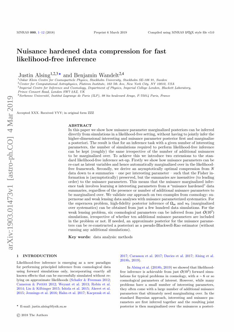
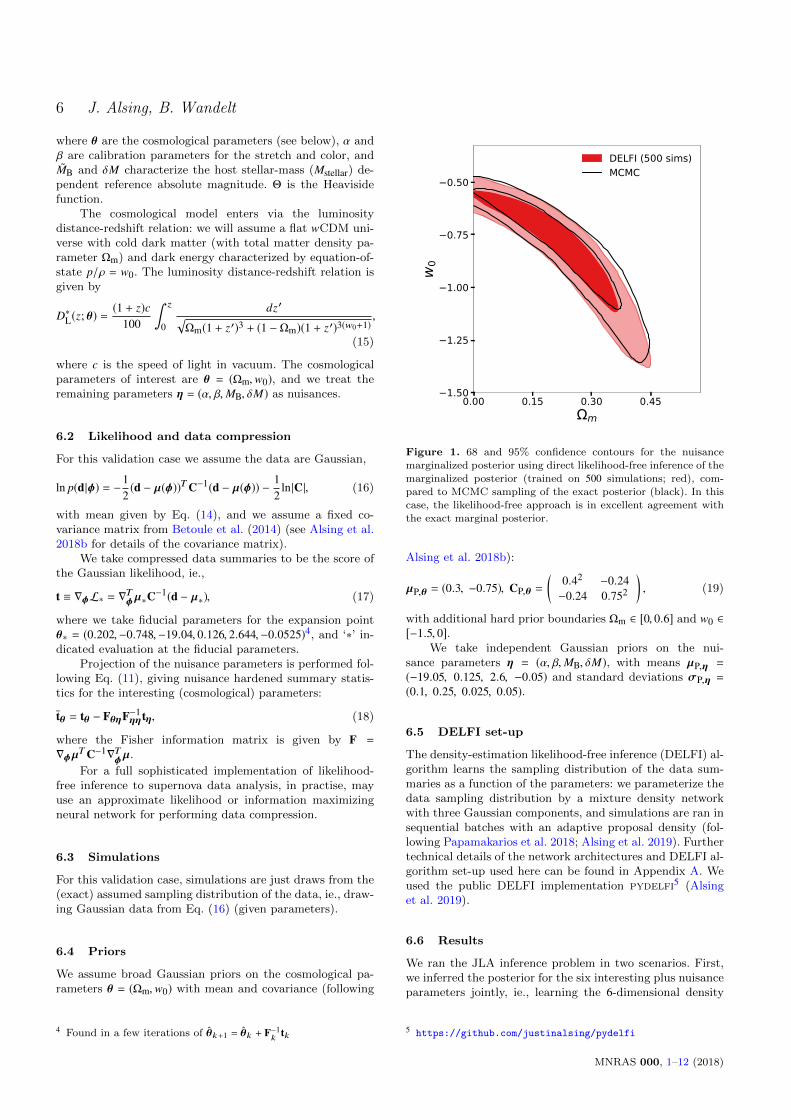
Figure 1. 68 and 95% confidence contours for the nuisancemarginalized posterior using direct likelihood-free inference of the

marginalized posterior (trained on 500 simulations; red), com-pared to MCMC sampling of the exact posterior (black). In this

case, the likelihood-free approach is in excellent agreement with

the exact marginal posterior.

Alsing et al. 2018b):

µP,θ = (0.3, −0.75), CP,θ =

(0.42 −0.24−0.24 0.752

), (19)

with additional hard prior boundaries Ωm ∈ [0, 0.6] and w0 ∈[−1.5, 0].

We take independent Gaussian priors on the nui-sance parameters η = (α, β, MB, δM), with means µP,η =(−19.05, 0.125, 2.6, −0.05) and standard deviations σP,η =(0.1, 0.25, 0.025, 0.05).

6.5 DELFI set-up

The density-estimation likelihood-free inference (DELFI) al-gorithm learns the sampling distribution of the data sum-maries as a function of the parameters: we parameterize thedata sampling distribution by a mixture density networkwith three Gaussian components, and simulations are ran insequential batches with an adaptive proposal density (fol-lowing Papamakarios et al. 2018; Alsing et al. 2019). Furthertechnical details of the network architectures and DELFI al-gorithm set-up used here can be found in Appendix A. Weused the public DELFI implementation pydelfi5 (Alsinget al. 2019).

6.6 Results

We ran the JLA inference problem in two scenarios. First,we inferred the posterior for the six interesting plus nuisanceparameters jointly, ie., learning the 6-dimensional density

5 https://github.com/justinalsing/pydelfi

MNRAS 000, 1–12 (2018)

https://github.com/justinalsing/pydelfi


(a) 2-parameter nuisance marginalized problem

200 400 600 800 1000 1200number of simulations, nsims

1

2

3

4

5

6

nega

tive

log

loss

, ln

U

training lossvalidation loss

(b) 6-parameter problem (including nuisance parameters)

0 2000 4000 6000 8000 10000 12000number of simulations, nsims

7

8

9

10

11

12

nega

tive

log

loss

, ln

U


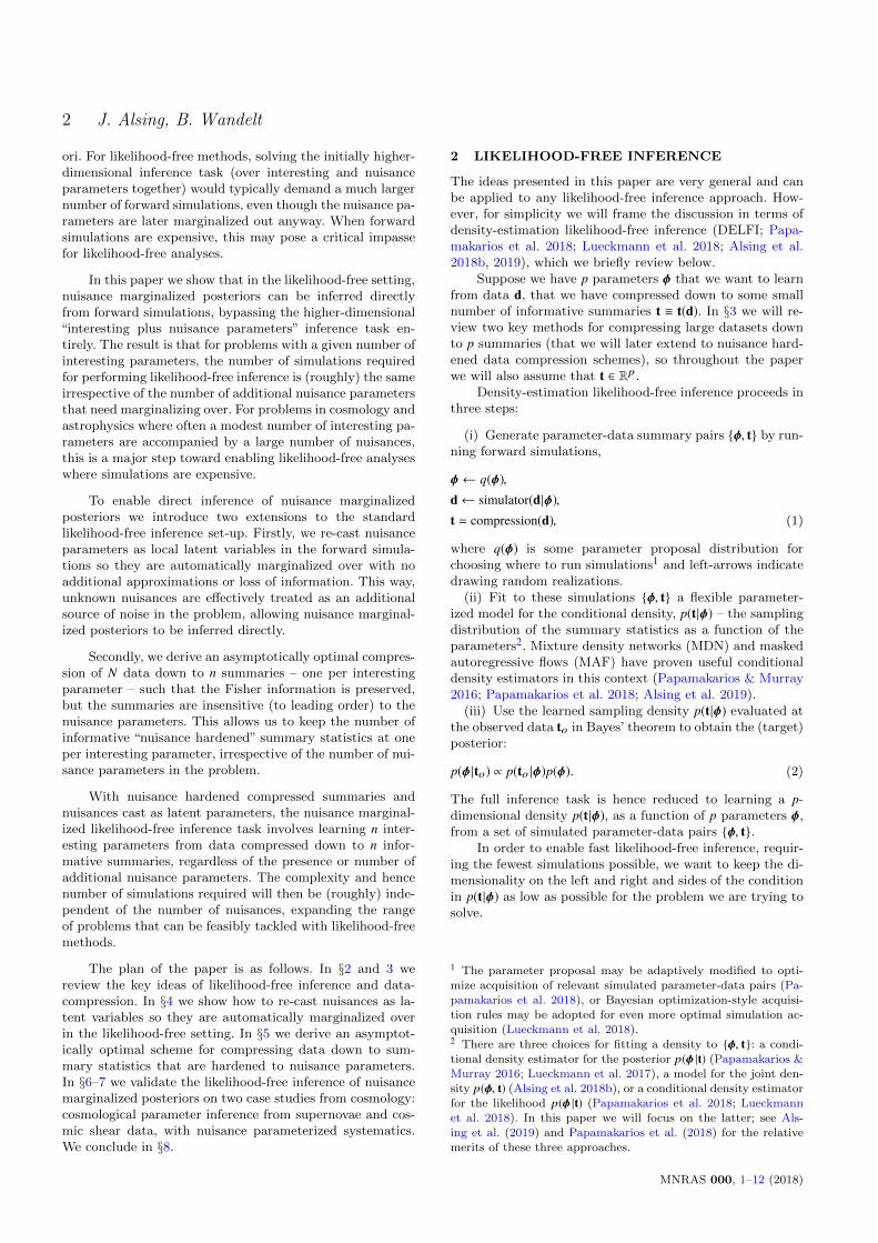
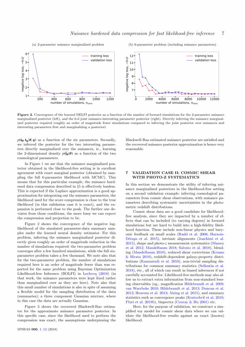
Figure 2. Convergence of the learned DELFI posterior as a function of the number of forward simulations for the 2-parameter nuisance

marginalized posterior (left), and the 6-d joint nuisance-interesting parameter posterior (right). Directly inferring the nuisance marginal-ized posterior required roughly an order of magnitude fewer simulations compared to inferring the joint posterior over nuisances and

interesting parameters first and marginalizing a posteriori.

p(tθ, tη |θ, η) as a function of the six parameters. Secondly,we inferred the posterior for the two interesting parame-ters directly marginalized over the nuisances, ie., learningthe 2-dimensional density p(tθ |θ) as a function of the twocosmological parameters.

In Figure 1 we see that the nuisance marginalized pos-terior obtained in the likelihood-free setting is in excellentagreement with exact marginal posterior (obtained by sam-pling the full 6-parameter likelihood with MCMC). Thismeans that for this particular example, the nuisance hard-ened data compression described in §5 is effectively lossless.This is expected if the Laplace approximation is a good ap-proximation for integrating out the nuisance parameters, thelikelihood used for the score compression is close to the truelikelihood (in this validation case it is exact), and the ex-pansion is performed close to the peak. The further one de-viates from those conditions, the more lossy we can expectthe compression and projection to be.

Figure 2 shows the convergence of the negative log-likelihood of the simulated parameter-data summary sam-ples under the learned neural density estimator. For thisproblem, inferring the nuisance marginalized posterior di-rectly gives roughly an order of magnitude reduction in thenumber of simulations required: the two-parameter problemconverges after a few hundred simulations, while the full six-parameter problem takes a few thousand. We note also thatfor the two-parameter problem, the number of simulationsrequired here is an order of magnitude fewer than was re-ported for the same problem using Bayesian OptimizationLikelihood-free Inference (BOLFI) in Leclercq (2018) (inthat work, the nuisance parameters were kept fixed ratherthan marginalized over as they are here). Note also thatthis small number of simulations is also in spite of assuminga flexible model for the sampling distribution of the data(summaries); a three component Gaussian mixture, wherein this case the data are actually Gaussian.

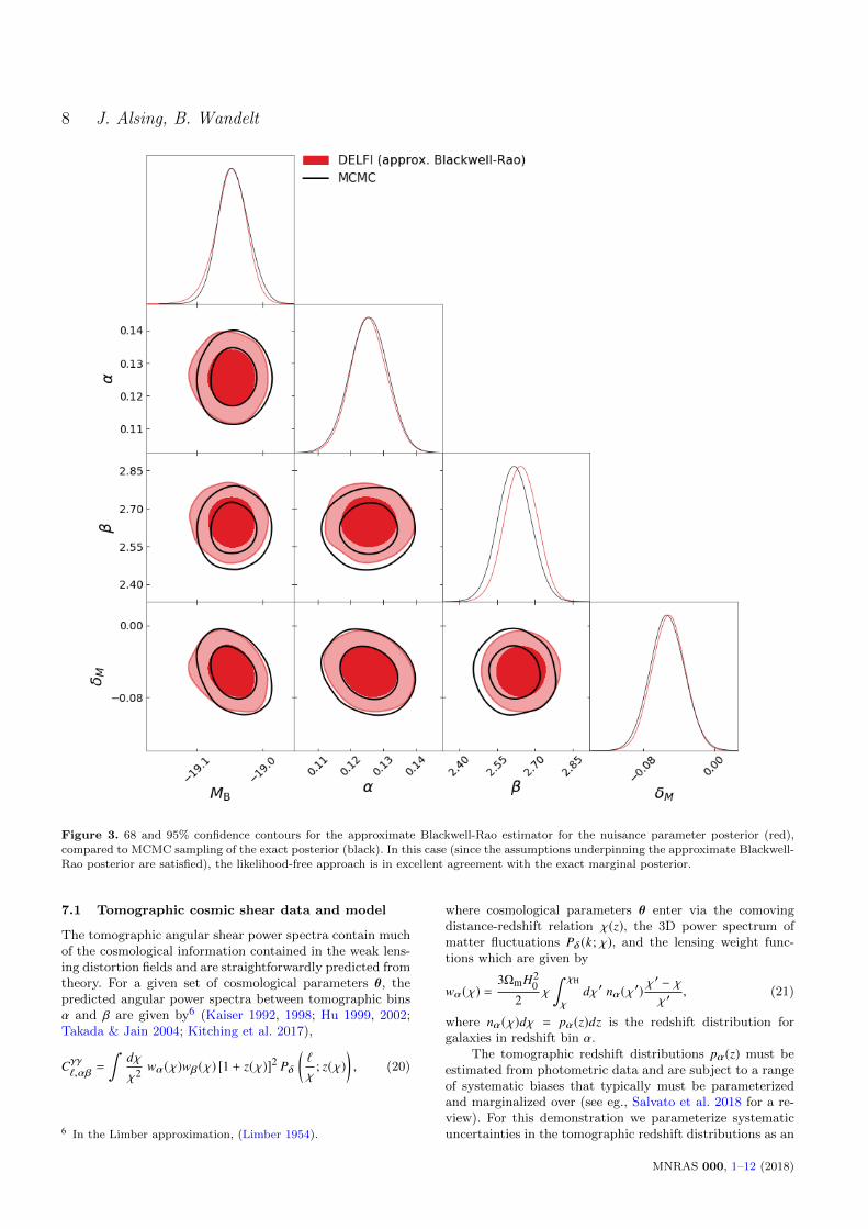
Figure 3 shows the recovered Blackwell-Rao estima-tor for the approximate nuisance parameter posterior. Inthis specific case, since the likelihood used to perform thecompression was exact, the assumptions underpinning the

Blackwell-Rao estimated nuisance posterior are satisfied andthe recovered nuisance posterior approximation is hence veryreasonable.

7 VALIDATION CASE II: COSMIC SHEARWITH PHOTO-Z SYSTEMATICS

In this section we demonstrate the utility of inferring nui-sance marginalized posteriors in the likelihood-free settingon a second validation example: inferring cosmological pa-rameters from cosmic shear observations, with nuisance pa-rameters describing systematic uncertainties in the photo-metric redshift distributions.

Cosmic shear data are a good candidate for likelihood-free analysis, since they are impacted by a number of ef-fects that can be included (to varying degrees) in forwardsimulations but are hard to build into a high-fidelity likeli-hood function. These include non-linear physics and bary-onic feedback on small scales (Rudd et al. 2008; Harnois-Deraps et al. 2015), intrinsic alignments (Joachimi et al.2015), shape and photo-z measurement systematics (Masseyet al. 2012; Mandelbaum 2018; Salvato et al. 2018), blend-ing (Mandelbaum 2018), reduced shear corrections (Krause& Hirata 2010), redshift-dependent galaxy-property distri-butions (Kannawadi et al. 2018), non-trivial sampling dis-tributions for common summary statistics (Sellentin et al.2018), etc., all of which can result in biased inferences if notcarefully accounted for. Likelihood-free methods may also al-low us to extract extra information from non-standard lens-ing observables (eg., magnification Hildebrandt et al. 2009;van Waerbeke 2010; Hildebrandt et al. 2013; Duncan et al.2013; Heavens et al. 2013; Alsing et al. 2015), and summarystatistics such as convergence peaks (Kratochvil et al. 2010;Fluri et al. 2018b), bispectra (Cooray & Hu 2001) etc.

Here, for the purpose of validation, we construct a sim-plified toy model for cosmic shear data where we can val-idate the likelihood-free results against an exact (known)likelihood.

MNRAS 000, 1–12 (2018)


Figure 3. 68 and 95% confidence contours for the approximate Blackwell-Rao estimator for the nuisance parameter posterior (red),compared to MCMC sampling of the exact posterior (black). In this case (since the assumptions underpinning the approximate Blackwell-Rao posterior are satisfied), the likelihood-free approach is in excellent agreement with the exact marginal posterior.

7.1 Tomographic cosmic shear data and model

The tomographic angular shear power spectra contain muchof the cosmological information contained in the weak lens-ing distortion fields and are straightforwardly predicted fromtheory. For a given set of cosmological parameters θ, thepredicted angular power spectra between tomographic binsα and β are given by6 (Kaiser 1992, 1998; Hu 1999, 2002;Takada & Jain 2004; Kitching et al. 2017),

Cγγ`,αβ

=

∫dχχ2 wα(χ)wβ(χ) [1 + z(χ)]2 Pδ

(`

χ; z(χ)

), (20)

6 In the Limber approximation, (Limber 1954).

where cosmological parameters θ enter via the comovingdistance-redshift relation χ(z), the 3D power spectrum ofmatter fluctuations Pδ(k; χ), and the lensing weight func-tions which are given by

wα(χ) =3ΩmH2

02

χ

∫ χH

χdχ′ nα(χ′)

χ′ − χχ′

, (21)

where nα(χ)dχ = pα(z)dz is the redshift distribution forgalaxies in redshift bin α.

The tomographic redshift distributions pα(z) must beestimated from photometric data and are subject to a rangeof systematic biases that typically must be parameterizedand marginalized over (see eg., Salvato et al. 2018 for a re-view). For this demonstration we parameterize systematicuncertainties in the tomographic redshift distributions as an

MNRAS 000, 1–12 (2018)


unknown shift of the estimated distributions, ie., setting

pα(z) = pα(z − bα), (22)

where pα(z) is the estimated redshift distribution for tomo-graphic bin α and the systematic shift parameters bα – oneper tomographic bin – constitute the nuisance parameters ηthat we ultimately want to marginalize over.

For this demonstration we will assume the data vectorto be a set of estimated (noise biased) band powers,

d = (CB1, CB2, . . . , CBK). (23)

We consider a flat-wCDM cosmology parameterized byθ = (σ8,Ωm,Ωbh2, h, ns,w0).

7.2 Likelihood and data compression

For this validation case study, we assume that the data(band powers) are independently Wishart distributed,

p(d|θ, η) =∏

bands, kW

(CBk

| CBk(θ, η), νBk

), (24)

where the elements of the expected band powers are givenby

CBk,i j =∑`∈Bk

(Cγγ`,i j(θ, η) + N`,i j )/νBk

. (25)

N`,i j is the shape noise power spectrum (from intrinsic ran-dom galaxy ellipticities) and νBk

is the total number ofmodes contributing to band k. We will assume isotropicshape noise N`,i j = σ2

e/niδi j with intrinsic ellipticity vari-

ance σ2e and mean galaxy number density ni in tomographic

bin i. We will assume νBk= fsky

∑`∈Bk

(2` + 1) modes perband to approximately mimick partial sky-fraction coveragefsky.

We take our compressed summaries as the score of theWishart likelihood in Eq. (24),

t ≡ ∇φL∗ =∑k

νBk

2tr[C−1Bk∗∇CBk∗C

−1Bk∗CBk

) − C−1Bk∗∇CBk∗

],

(26)

where ‘∗’ indicates evaluation about fiducial parameters θ∗which we take to be θ∗ = (0.8, 0.3, 0.05, 0.7, 0.96,−1).

Projection of the nuisance parameters is performed fol-lowing Eq. (11) as usual, giving nuisance hardened summarystatistics:

tθ = tθ − FθηF−1ηηtη, (27)

where the Fisher matrix in this case is given by,

F∗ = −〈∇θ∇Tθ L〉∗ =∑k

νBk

2tr[C−1Bk∗∇θCBk∗C

−1Bk∗∇

Tθ CBk∗

].

(28)

For a full sophisticated implementation of likelihood-free inference to cosmic shear on real data, an approximatelikelihood or information maximizing neural network maybe used for performing data compression.

7.3 Simulations

In this simple validation case we simulate data (given param-eters) by drawing band powers as Wishart random variates,following Eq. (24).

0 2000 4000 6000 8000 10000 12000number of simulations, nsims

1

0

1

2

nega

tive

log

loss

, ln

U


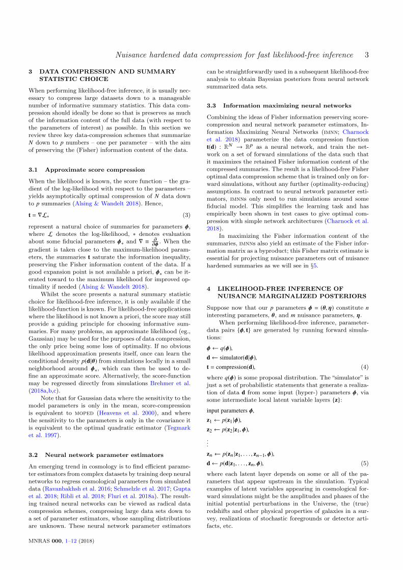
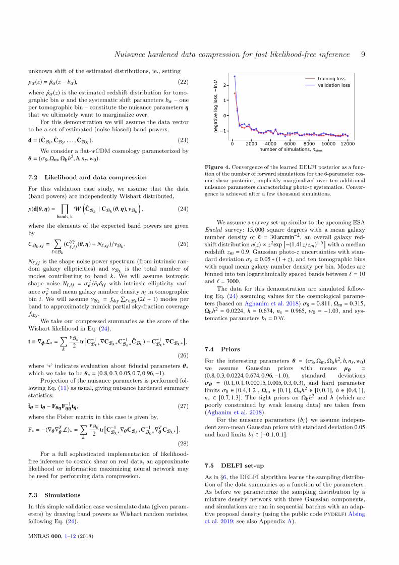
Figure 4. Convergence of the learned DELFI posterior as a func-tion of the number of forward simulations for the 6-parameter cos-

mic shear posterior, implicitly marginalized over ten additional

nuisance parameters characterizing photo-z systematics. Conver-gence is achieved after a few thousand simulations.

We assume a survey set-up similar to the upcoming ESAEuclid survey: 15, 000 square degrees with a mean galaxynumber density of n = 30 arcmin−2, an overall galaxy red-shift distribution n(z) ∝ z2exp

[−(1.41z/zm)1.5

]with a median

redshift zm = 0.9, Gaussian photo-z uncertainties with stan-dard deviation σz = 0.05 ∗ (1 + z), and ten tomographic binswith equal mean galaxy number density per bin. Modes arebinned into ten logarithmically spaced bands between ` = 10and ` = 3000.

The data for this demonstration are simulated follow-ing Eq. (24) assuming values for the cosmological parame-ters (based on Aghanim et al. 2018) σ8 = 0.811, Ωm = 0.315,Ωbh2 = 0.0224, h = 0.674, ns = 0.965, w0 = −1.03, and sys-tematics parameters bi = 0 ∀i.

7.4 Priors

For the interesting parameters θ = (σ8,Ωm,Ωbh2, h, ns,w0)we assume Gaussian priors with means µθ =

(0.8, 0.3, 0.0224, 0.674, 0.96,−1.0), standard deviationsσθ = (0.1, 0.1, 0.00015, 0.005, 0.3, 0.3), and hard parameterlimits σ8 ∈ [0.4, 1.2], Ωm ∈ [0, 1], Ωbh2 ∈ [0, 0.1], h ∈ [0.4, 1],ns ∈ [0.7, 1.3]. The tight priors on Ωbh2 and h (which arepoorly constrained by weak lensing data) are taken from(Aghanim et al. 2018).

For the nuisance parameters bi we assume indepen-dent zero-mean Gaussian priors with standard deviation 0.05and hard limits bi ∈ [−0.1, 0.1].

7.5 DELFI set-up

As in §6, the DELFI algorithm learns the sampling distribu-tion of the data summaries as a function of the parameters.As before we parameterize the sampling distribution by amixture density network with three Gaussian components,and simulations are ran in sequential batches with an adap-tive proposal density (using the public code pydelfi Alsinget al. 2019; see also Appendix A).

MNRAS 000, 1–12 (2018)


1.35

1.05

0.75

w0

0.760.780.800.820.84

8

0.048

0.052

b

0.656

0.672

0.688

h

0.900.930.960.991.02

n s

0.25

0.30

0.35

m

1.35

1.05

0.75

w0

0.760.7

80.8

00.8

20.8

4

80.0

480.0

52

b0.6

560.6

720.6

88

h0.9

00.9

30.9

60.9

91.0

2

ns

DELFI (2000 sims)MCMC

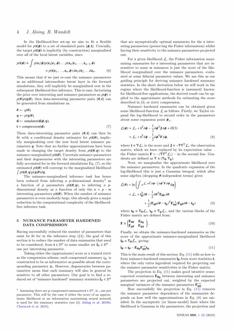
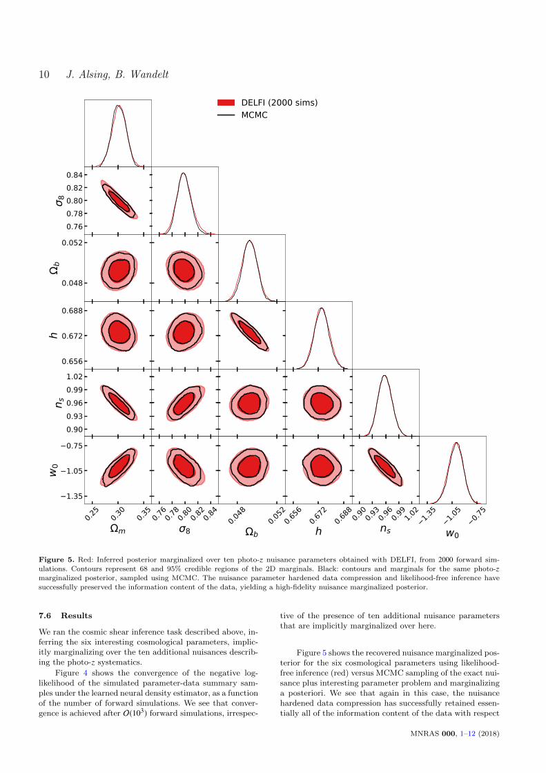
Figure 5. Red: Inferred posterior marginalized over ten photo-z nuisance parameters obtained with DELFI, from 2000 forward sim-

ulations. Contours represent 68 and 95% credible regions of the 2D marginals. Black: contours and marginals for the same photo-zmarginalized posterior, sampled using MCMC. The nuisance parameter hardened data compression and likelihood-free inference have

successfully preserved the information content of the data, yielding a high-fidelity nuisance marginalized posterior.

7.6 Results

We ran the cosmic shear inference task described above, in-ferring the six interesting cosmological parameters, implic-itly marginalizing over the ten additional nuisances describ-ing the photo-z systematics.

Figure 4 shows the convergence of the negative log-likelihood of the simulated parameter-data summary sam-ples under the learned neural density estimator, as a functionof the number of forward simulations. We see that conver-gence is achieved after O(103) forward simulations, irrespec-

tive of the presence of ten additional nuisance parametersthat are implicitly marginalized over here.

Figure 5 shows the recovered nuisance marginalized pos-terior for the six cosmological parameters using likelihood-free inference (red) versus MCMC sampling of the exact nui-sance plus interesting parameter problem and marginalizinga posteriori. We see that again in this case, the nuisancehardened data compression has successfully retained essen-tially all of the information content of the data with respect

MNRAS 000, 1–12 (2018)


to the interesting parameters, yielding a high-fidelity nui-sance marginalized (likelihood-free) posterior inference.

8 CONCLUSIONS

We have shown that nuisance marginalized posteriors canbe inferred directly in the likelihood-free paradigm, mas-sively reducing the number of simulations required to per-form likelihood-free inference in the presence of nuisance pa-rameters. This opens up likelihood-free methods to problemswith expensive forward simulations, a small number of pa-rameters of interest, but a large number of additional nui-sance parameters; a common scenario in cosmological dataanalysis.

To achieve fast direct inference of nuisance marginal-ized posteriors, we do the following: first, we showed thatnuisance parameters can easily be re-cast as local latentvariables and hence implicitly marginalized over in thelikelihood-free inference framework (§4). Secondly, we de-rived a scheme for compressing N data down to n infor-mative summaries – one per parameter of interest – suchthat the compressed summaries (asymptotically) retain theFisher information content of the data for the interestingparameters whilst being “hardened” to the nuisance param-eters. This means that just n data summaries can be usedfor likelihood-free inference, regardless of the number of nui-sance parameters.

The result is that the complexity of the inference task –and hence the number of simulations required for performinginference – is dictated only by the number of interestingparameters considered in the problem.

ACKNOWLEDGEMENTS

This work is supported by the Simons Foundation. JustinAlsing was partially supported by the research project grant“Fundamental Physics from Cosmological Surveys” fundedby the Swedish Research Council (VR) under Dnr 2017-04212. Benjamin Wandelt acknowledges support by theLabex Institut Lagrange de Paris (ILP) (reference ANR-10-LABX-63) part of the Idex SUPER, and received financialstate aid managed by the Agence Nationale de la Recherche,as part of the programme Investissements d’avenir under thereference ANR-11-IDEX-0004-02.

REFERENCES

Aghanim N., et al., 2018, arXiv preprint arXiv:1807.06209

Akeret J., Refregier A., Amara A., Seehars S., Hasner C., 2015,

Journal of Cosmology and Astroparticle Physics, 2015, 043

Alsing J., Wandelt B., 2018, Monthly Notices of the Royal Astro-

nomical Society: Letters, 476, L60

Alsing J., Kirk D., Heavens A., Jaffe A. H., 2015, Monthly Noticesof the Royal Astronomical Society, 452, 1202

Alsing J., Wandelt B. D., Feeney S. M., 2018a, arXiv preprint

arXiv:1808.06040

Alsing J., Wandelt B., Feeney S., 2018b, Monthly Notices of theRoyal Astronomical Society, 477, 2874

Alsing J., Charnock T., Feeney S., Wandelt B., 2019, pre-print

arXiv:1903.00007

Betoule M. e. a., et al., 2014, Astronomy & Astrophysics, 568,

A22

Brehmer J., Cranmer K., Louppe G., Pavez J., 2018b, arXiv

preprint arXiv:1805.00013

Brehmer J., Cranmer K., Louppe G., Pavez J., 2018c, arXiv


Brehmer J., Louppe G., Pavez J., Cranmer K., 2018a, arXiv


Cameron E., Pettitt A., 2012, Monthly Notices of the Royal As-

tronomical Society, 425, 44

Carassou S., de Lapparent V., Bertin E., Borgne D. L., 2017,

arXiv preprint arXiv:1704.05559

Charnock T., Lavaux G., Wandelt B. D., 2018, Physical Review

D, 97, 083004

Cooray A., Hu W., 2001, The Astrophysical Journal, 548, 7

Davies F. B., Hennawi J. F., Eilers A.-C., Lukic Z., 2017, arXiv


Duncan C. A. J., Joachimi B., Heavens A. F., Heymans C., Hilde-

brandt H., 2013, Monthly Notices of the Royal AstronomicalSociety, 437, 2471

Fluri J., Kacprzak T., Lucchi A., Refregier A., Amara A., Hof-mann T., 2018a, arXiv preprint arXiv:1807.08732

Fluri J., Kacprzak T., Sgier R., Refregier A., Amara A., 2018b,arXiv preprint arXiv:1803.08461

Gupta A., Matilla J. M. Z., Hsu D., Haiman Z., 2018, PhysicalReview D, 97, 103515

Hahn C., Vakili M., Walsh K., Hearin A. P., Hogg D. W., Camp-

bell D., 2017, Monthly Notices of the Royal Astronomical So-

ciety, 469, 2791

Harnois-Deraps J., van Waerbeke L., Viola M., Heymans C., 2015,

Monthly Notices of the Royal Astronomical Society, 450, 1212

Heavens A. F., Jimenez R., Lahav O., 2000, Monthly Notices of

the Royal Astronomical Society, 317, 965

Heavens A., Alsing J., Jaffe A., 2013, arXiv.org

Hildebrandt H., van Waerbeke L., Erben T., 2009, preprint, 507,

683

Hildebrandt H., et al., 2013, MNRAS, astro-ph.CO, 488

Hu W., 1999, ApJ, 522, L21

Hu W., 2002, Phys. Rev. D, 65, 023003

Ishida E., et al., 2015, Astronomy and Computing, 13, 1

Jennings E., Wolf R., Sako M., 2016, arXiv preprint

arXiv:1611.03087

Joachimi B., et al., 2015, Space Science Reviews, 193, 1

Kacprzak T., Herbel J., Amara A., Refregier A., 2017, arXivpreprint arXiv:1707.07498

Kaiser N., 1992, The Astrophysical Journal, 388, 272

Kaiser N., 1998, The Astrophysical Journal, 498, 26

Kannawadi A., et al., 2018, arXiv e-prints

Kingma D. P., Ba J., 2014, arXiv preprint arXiv:1412.6980

Kitching T. D., Alsing J., Heavens A. F., Jimenez R., McEwenJ. D., Verde L., 2017, Monthly Notices of the Royal Astro-nomical Society, 469, 2737

Kratochvil J. M., Haiman Z., May M., 2010, Physical Review D,

81, 043519

Krause E., Hirata C. M., 2010, Astronomy & Astrophysics, 523,

A28

Leclercq F., 2018, arXiv preprint arXiv:1805.07152

Limber D. N., 1954, The Astrophysical Journal, 119, 655

Lin C.-A., Kilbinger M., 2015, Astronomy & Astrophysics, 583,A70

Lueckmann J.-M., Goncalves P. J., Bassetto G., Ocal K., Non-nenmacher M., Macke J. H., 2017, in Advances in Neural In-

formation Processing Systems. pp 1289–1299

Lueckmann J.-M., Bassetto G., Karaletsos T., Macke J. H., 2018,

arXiv preprint arXiv:1805.09294

Mandelbaum R., 2018, Annual Review of Astronomy and Astro-

physics, 56, 393

Massey R., et al., 2012, preprint, astro-ph.CO

MNRAS 000, 1–12 (2018)


Papamakarios G., Murray I., 2016, in Advances in Neural Infor-

mation Processing Systems. pp 1028–1036

Papamakarios G., Sterratt D. C., Murray I., 2018, arXiv preprint

arXiv:1805.07226

Ravanbakhsh S., Oliva J. B., Fromenteau S., Price L., Ho S.,Schneider J. G., Poczos B., 2016, in ICML. pp 2407–2416

Ribli D., Pataki B. A., Csabai I., 2018, arXiv preprint

arXiv:1806.05995

Robin A., Reyle C., Fliri J., Czekaj M., Robert C., Martins A.,

2014, Astronomy & Astrophysics, 569, A13

Rudd D. H., Zentner A. R., Kravtsov A. V., 2008, The Astro-

physical Journal, 672, 19

Salvato M., Ilbert O., Hoyle B., 2018, arXiv preprintarXiv:1805.12574

Schafer C. M., Freeman P. E., 2012, in , Statistical Challenges in

Modern Astronomy V. Springer, pp 3–19

Schmelzle J., Lucchi A., Kacprzak T., Amara A., Sgier

R., Refregier A., Hofmann T., 2017, arXiv preprintarXiv:1707.05167

Sellentin E., Heymans C., Harnois-Deraps J., 2018, Monthly No-

tices of the Royal Astronomical Society, 477, 4879

Takada M., Jain B., 2004, MNRAS, 348, 897

Tegmark M., Taylor A. N., Heavens A. F., 1997, The Astrophys-

ical Journal, 480, 22

Tripp R., 1998, Astronomy and Astrophysics, 331, 815

Weyant A., Schafer C., Wood-Vasey W. M., 2013, The Astrophys-

ical Journal, 764, 116

Zablocki A., Dodelson S., 2016, Physical Review D, 93, 083525

van Waerbeke L., 2010, MNRAS, 401, 2093

APPENDIX A: DELFI ALGORITHM SET-UP

We parameterize the sampling distribution of the data sum-maries p(t|θ) as a mixture density network. Simulations arerun in batches and the mixture network is re-trained aftereach new batch of simulations. In the first cycle, parametersfor performing forward simulations are drawn from a broadGaussian centered on the prior mean and with covarianceequal to nine times the (estimated) Fisher matrix. For sub-sequent batches of simulations, parameters are drawn fromthe geometric mean of the current posterior estimate fromthe mixture network and the prior7.

The neural networks are trained using the stochasticgradient optimizer adam (Kingma & Ba 2014), with a batch-size of one tenth of the training set during each re-trainingcycle and a learning rate of 0.001. Over-fitting is preventedduring training using early-stopping; during each re-trainingcycle, 10% of the training set is set aside for validation andtraining is terminated when the validation-loss does not im-prove after 20 epochs.

We set the size of the mixture network architecture andnumber of new simulations per training cycle depending onthe number of parameters to be inferred. We use the follow-ing rule of thumb for scaling the architecture and simulationbatches: all of the networks have two hidden layers with 5×as many units as parameters to be inferred, and simulationsare run in batches of 50× the number of parameters in the

7 This proposal density is inspired by the optimal parameterproposal for Approximate Bayesian Computation (Alsing et al.

2018a).

problem. Of course, this is a very rough heuristic and care-ful application of neural density estimators should involve across-validation search over network architectures.

This paper has been typeset from a TEX/LATEX file prepared by

the author.

MNRAS 000, 1–12 (2018)

nuisance hardened data compression for fast likelihood

Documents