nudging to reduce meat consumption: immediate and
TRANSCRIPT

ISSN 1403-2473 (Print) ISSN 1403-2465 (Online)
Working Paper in Economics No. 712
Nudging to reduce meat consumption: Immediate and persistent effects of an intervention at a university restaurant Verena Kurz Department of Economics, November 2017

Nudging to reduce meat consumption: Immediate and persistent effects of an intervention at a university restaurant*
Verena Kurz‡
November 6, 2017
Abstract
Changing dietary habits to reduce the consumption of meat is considered to have great poten-tial to mitigate food-related greenhouse gas (GHG) emissions. To test if nudging can increase the consumption of vegetarian food, I conducted a field experiment with two university res-taurants. At the treated restaurant, the salience of the vegetarian option was increased by changing the menu order, and by placing the dish at a spot visible to customers. The other restaurant served as a control. Daily sales data on the three main dishes sold were collected from September 2015 until June 2016. The experiment was divided into a baseline, an inter-vention, and a reversal period where the setup was returned to its original state. Results show that the nudge increased the share of vegetarian lunches sold by around 6 percentage points. The change in behavior is partly persistent, as the share of vegetarian lunches sold remained 4 percentage points higher than during the baseline period after the original setup was reinstat-ed. The changes in consumption reduced GHG emissions from food sales around 5 percent.
Keywords: nudging, field experiment, meat consumption, climate change mitigation
JEL classification: D12, C93, Q50, D03
* I thank Eurest Restaurants at Gothenburg University, especially Krister Johansson, Harald Boye, and Mikael Börjesson, for facilitating this field experiment and providing the data. Many thanks to Randi Hjalmarsson, Fred-rik Carlsson, Nadine Ketel, Gerlinde Fellner-Röhling, Simon Felgendreher, seminar participants at the Universi-ty of Gothenburg, and participants at the 2016 Nordic Conference in Behavioral and Experimental Economics in Oslo and the 2016 Advances with Field Experiments Conference in Chicago for helpful comments. Any remain-ing errors are my own. Financial support from the Swedish Environmental Protection Agency is gratefully acknowledged. ‡Department of Economics, University of Gothenburg, Sweden, [email protected].

2
1. Introduction
This paper presents results from a field experiment using a nudge with the aim of increas-
ing the share of vegetarian lunches sold at a university restaurant. Changing diets to reduce
consumption of meat and dairy is seen as an important part of mitigation efforts to reach a 2-
degree climate target (Bryngelsson et al., 2016; Girod et al., 2014). The livestock sector con-
tributes approximately 14.5 percent of global human-induced greenhouse gas (GHG) emis-
sions yearly (Gerber et al., 2013), and meat consumption is causing about one-third of food-
related GHG emissions emerging from consumption in Western countries such as Sweden and
the United States (Jones and Kammen, 2011; Naturvårdsverket, 2011).1 Reducing meat con-
sumption is also seen as a way to protect biodiversity, land, and freshwater ecosystems
(Machovina and Feeley, 2014; Pelletier and Tyedmers, 2010; Pimentel and Pimentel, 2003).
Moreover, a reduction in meat consumption can yield significant benefits for both public
health and the environment (Springmann et al., 2016; Tilman and Clark, 2014; Westhoek et
al., 2014), mainly by decreasing the risk of colorectal cancer, type 2 diabetes, and cardiovas-
cular diseases (Swedish National Food Agency, 2015).
However, as data from Sweden where this field experiment took place, shows, reducing
meat consumption will be challenging: per capita consumption has constantly risen since the
1990s to a record-high 87.7 kilograms (kg) per person in 2016 (Swedish Agricultural Board,
2017). Under the absence of price instruments such as meat taxes, one suggestion gaining
popularity in the literature is to use nudging as a cheap and nondistortionary strategy to
change consumer behavior towards less carbon-intensive consumption patterns (Girod et al.,
2014; Lehner et al., 2016; Sunstein, 2015).2 A nudge is commonly understood as a soft push
toward behavior that is judged to be desirable by individuals or policy makers but that has not
been fully adopted. Such a soft push can be implemented through small changes in the deci-
sion environment, while prices and the choice set remain unchanged (Thaler and Sunstein,
2008). Most nudges build on a dual process model of cognition, which models human behav-
1 In general, food is responsible for around one-fourth of the consumption-based emissions of an average US household. For Sweden, emissions from consumption are available not on a household but on an individual ba-sis: approximately 8 tons of CO2 equivalent (tCO2e) per capita emerge from private consumption, of which 2 tCO2e relate to food. Of those, 0.7 tCO2e can be attributed to meat consumption (Naturvårdsverket, 2011). 2 Alternative policy instruments such as food consumption taxes based on GHG emissions have been discussed by the scientific community, but implementation is not foreseeable yet (Säll and Gren, 2015; Wirsenius et al., 2011). Carbon labeling has also been discussed as a possibility to reduce meat consumption. See Shewmake et al. (2015) for a theoretical analysis and Visschers and Siegrist (2015) and Vlaeminck et al. (2014) for empirical tests.

3
ior as governed by two modes of thinking and deciding (Kahneman, 2003, 2011). Decisions
dominated by the first mode, also called system one, are characterized by an intuitive, fast,
and automatic style of thinking where cognitive effort is low. In the second mode, or system
two, slow, reflective, and controlled processes, which require more cognitive effort, dominate.
Nudging often targets decisions dominated by system one, where cognitive effort is low and
the decision environment is of high importance. Food choices are seen as classical examples
of decisions governed by system one where the choice environment, such as the salience of
items, the structure of food assortments, or the packaging, matters (Cohen and Farley, 2007;
Marteau et al., 2012; Wansink and Sobal, 2007). In this experiment, I test whether nudging
can reduce meat consumption during lunch by altering two aspects of a restaurant’s physical
environment: the order in which the dishes are presented on the menu and the visibility of the
vegetarian dish. Moreover, I analyze the effect of the nudge on consumption choices over
time and test whether the nudge has any persistent effects after the intervention ends.
To date, few field experiments have actually tested the efficacy of nudging to reduce envi-
ronmental impacts from consumption. Examples include the use of social norms to reduce
household water and electricity consumption (Allcott, 2011; Ferraro and Price, 2013; Jaime
Torres and Carlsson, 2016) and changing the default setting of office printers to duplex to
reduce paper consumption (Egebark and Ekström, 2016). The evidence for nudging as a tool
to facilitate healthier food choices is broader and mostly comes from experiments changing
aspects of the physical environment, such as the menu order or the convenience of ordering
unhealthy items (Dayan and Bar-Hillel, 2011; Just, 2009; Rozin et al., 2011; Wisdom et al.,
2010). However, there is no evidence as to whether nudging also works to induce more envi-
ronmentally friendly food choices. Conceptually, nudging for the environment may be very
different from nudging for health: while nudging healthy choices is often motivated by the
idea of inconsistent individual preferences such as present bias, which causes people to
choose unhealthy options in the present that they will regret in the future (see, for example,
Wisdom et al., 2010), it is not clear that such cognitive biases exist with respect to the sus-
tainability of food choices. With regard to the high observed levels of meat consumption, it
could well be that people’s preferences are coherent, reducing the potential of nudging as a
strategy to change choices. Another aspect that can reduce the effect nudging has on choices
are strong underlying preferences for the good that the nudge is intended to reduce consump-
tion of. For example, Wansink and Just (2016) find that children opted out from the default
option of apples as a side dish and chose French fries. Wijk et al. (2016) find that increasing
the accessibility of whole grain bread compared to white bread did not increase its sales.

4
There is some suggestive evidence that Swedes would like to reduce their meat consump-
tion but fail to do so. In a representative World Wildlife Fund (WWF) survey, 37 percent of
the respondents state that they will cut their meat consumption in order to reduce their climate
impact during the coming year, and 33 percent state that they have already done so during the
previous year (WWF, 2016). At the same time, Swedish meat consumption rose to an all-time
high in 2016 (Swedish Agricultural Board, 2017). Whether preferences for meat are simply
too strong for nudging to help overcome a potential intentions-behavior gap is thus an im-
portant question to examine.
The experiment took place at two university restaurants in Gothenburg, Sweden, with one
serving as the treated restaurant and the other as a control. Both are run by the same provider
and serve three warm dishes during lunch, one vegetarian and two containing either meat or
fish. Daily sales data on the number of each of the three main dishes sold were collected from
September 2015 until June 2016, covering the whole academic year. The first nine weeks
served as a baseline period, followed by an intervention period of 17 weeks at the treated res-
taurant, where the vegetarian option was moved from the middle to the top of the printed
menu, and the dish was moved from behind the counter to a spot visible to customers at the
point of decision-making. Thus both the menu order and the visibility of the vegetarian dish
were changed simultaneously. However, we have some evidence for the effect of changing
the menu order only, as the local chef changed the menu order for five nonconsecutive weeks
during spring 2016 at the control restaurant. During the final 13 weeks of the year, the origi-
nal setup was reinstated at the treated restaurant.
Previous experiments have focused on the immediate impacts of nudges on food consump-
tion, but it is important to study longer time periods to evaluate their overall effect.3 One con-
cern with nudging is that it might have only short-term effects that quickly disappear once
people gain experience with the good or the choice setting (Croson and Treich, 2014; Löfgren
et al., 2012; Lusk, 2014). In the present experiment, this could be the case if customers were
initially nudged to choose the vegetarian option but returned to their original choices once
they became accustomed to the new setting, either because they did not like the vegetarian
3 Previous experiments on food nudges (for example, Dayan and Bar-Hillel , 2011; Just, 2009; Rozin et al., 2011; Wisdom et al., 2010) mainly were conducted in places that customers were not expected to visit repeatedly, such as diners or hotels; in other cases (for example, Policastro et al., 2015), the intervention was done too infrequent-ly to analyze effects over time.

5
option or because the nudge initially increased the number of ordering mistakes.4 The effect
of the nudge could also increase over time, such as if people recommend eating vegetarian to
fellow students after trying it as a result of the nudge. A priori, it is not clear whether and how
the impact of the nudge changes over time. Combining an intervention period of 17 weeks
and a customer pool that can be assumed to be fairly constant throughout the academic year,
this is the first experiment that allows for studying the effects of a food nudge over time.
Another important question is whether the nudge affects choices only during the interven-
tion period or has a persistent impact on behavior after it is removed. To date, no studies have
looked at the habit-forming effects of nudges in the food domain.5 If present utility of con-
suming a good depends on past levels of consumption, such as in the habit formation models
of Becker and Murphy (1988) or Naik and Moore (1996), an initial increase of vegetarian
lunches sold because of the nudge can lead to subsequent further increases. Empirical studies
show habit formation for a range of foods (see Daunfeldt et al., 2011, for an overview), but
results from experiments using incentives to increase healthier food choices are inconclusive.
Consuption of targeted items is usually somewhat higher immediately after the end of an in-
tervention than prior to it (Just and Price, 2013; List and Samek, 2015, 2017). Loewenstein et
al. (2016) even find a persistent effect one and three months after the end of an incentive
scheme, while Just and Price (2013) and Belot et al. (2015) do not find any persistent effects
of incentives in the medium run. Nudging could be a more promising approach to creating
new habits than incentivizing choices, as it does not carry the risk of crowding out intrinsic
motivation (Gneezy et al., 2011). On the other hand, habit formation could be even less pro-
nounced when using nudging, as a subtle intervention targeting the decision environment
might be less successful in causing behavior change in the first place. To examine if any ef-
fect of the nudge persisted after removing it, the original setup at the treated restaurant was
reinstated for the last 13 weeks of the academic year.
Results show that when using a difference-in-differences approach to estimate the treat-
ment effect, the combined nudge of changing visibility and menu order increased the average
4 This could occur if people simply point toward the dish that is most visible and assume it is the usual meat or fish dish served, or if they read off the first item on the menu. In an international environment such as the Uni-versity of Gothenburg, with many foreign employees and students that do not speak Swedish, simply reading off the first item on the menu could be a reasonable strategy if this had been successful in the past. Although an English menu is also provided, the Swedish menu is the one that features most prominently in the restaurants. 5 Persistent effects of behavioral interventions on water and electricity consumption have been found by studies such as Ferraro et al. (2011) and Allcott and Rogers (2014). However, as Brandon et al. (2017) discuss, these long-term effects are most likely due to an adjustment of physical capital.

6
sales share of vegetarian lunches by around 6 percentage points during the intervention peri-
od. Analyzing the treatment effect over time shows an increase over the course of the inter-
vention, suggesting that the average effect is not due to initial ordering mistakes or a one-off
effect of trying vegetarian food. Rather, it seems as if customers learn about the vegetarian
option, and some then incorporate it permanently into their choice set. Support for this argu-
ment also comes from the postintervention period, when the original setup was reinstated and
the share of vegetarian lunches sold persisted in being 4 percentage points higher than before
the intervention. Back-of-the-envelope calculations of the effect of the intervention on GHG
emissions show that the nudge decreased total emissions by around 5 percent.
2. The experiment
2.1. Experimental design
The experimental design targets the visibility of the vegetarian dish and the menu order,
two features of the food environment that have been shown to matter for food choice. Chang-
ing the visibility can affect whether and how prominently a dish features in the consideration
set (Wansink and Love, 2014). If customers might not even consider the vegetarian dish an
option and routinely choose between the two meat dishes offered, making it visible can add it
to the consideration set without changing what is offered. Enhanced visibility will also in-
crease a dish’s saliency—that is, how much it attracts attention and how prominently it fea-
tures in decision-making (Cohen and Farley, 2007; Wansink and Sobal, 2007). Third, chang-
ing which dish is visible at the point of purchasing can also change the customers’ infor-
mation about a dish. If vegetarian dishes are unknown by name to a majority of consumers,
making the dish visible can help them evaluate the vegetarian option before making a choice.
Changing the order in which the three lunch options are presented on the menu relies on
findings from previous research showing that when people are choosing from a list, order ef-
fects can bias them toward selecting specific objects with a higher likelihood. Primacy effects
increase the likelihood that they will choose items listed first. Such effects can arise if people
exhibit a confirmatory bias, such as looking for reasons to choose an alternative rather than
for reasons not to choose it, because of growing fatigue when reading through a list, or as a
result of satisficing behavior, where options are evaluated as generally similar and reading
through a whole list entails higher costs than benefits (Carney and Banaji, 2012; Mantonakis
et al., 2009; Miller and Krosnick, 1998). Dayan and Bar-Hillel (2011) study the influence of
menu order on choices in a coffee shop and find that placing an item at one of the extreme

7
positions (top or bottom) increases its sales by approximately 20 percent compared with when
the same item appears in the middle. Policastro et al. (2015) study the order of an ingredients
list on an ordering form and find that putting healthy items at the top of each ingredient cate-
gory leads to healthier self-assembled sandwiches.6
The experiment was conducted at two restaurants at the University of Gothenburg during
the academic year 2015–16. Gothenburg is the second largest city in Sweden, with a popula-
tion around 550,000, and its university is the fourth largest in the country, with about 24,000
full-time students. The departments of the university are spread across the city, and the uni-
versity buildings that hosted the experiment are approximately 2.5 kilometers (km) away from
each other. Both restaurants serve three warm alternatives during lunch: one vegetarian and
two including either meat or fish (called “meat 1” and “meat 2” in the following).7 The restau-
rants are subject to the same management, but the local chefs decide on the weekly menus,
and hence they differ across restaurants. Prices, however, are the same: warm dishes cost 70
SEK (approximately €7.30 or US$7.80) and are accompanied by bread, salad, and water. In-
stead of a warm dish, customers can also opt for soup, various salads, or sandwiches, which
are priced differently. At both restaurants, the menu for the whole week is posted at the en-
trance but only the daily menu is shown at the point of ordering. Many employees and stu-
dents also subscribe to the restaurant’s weekly menu by email.
Restaurant 1, the treated restaurant where the nudge was implemented, is in a building that
houses the economics, business administration, and law faculty. Hence, students and faculty
members eating there mainly belong to those disciplines. Restaurant 2, which serves as a con-
trol where no changes were undertaken, is in a building housing mostly institutions belonging
to the humanities. To capture initial differences between the restaurants in the quantity of
vegetarian food consumed, the academic year was divided into three experimental periods.
Period 0, the baseline or control period, lasted from September 1 until November 8 (10
weeks). The intervention period (period 1) lasted from November 9 until March 6 (17 weeks
including Christmas break). From March 7 until June 3 (13 weeks), the intervention ended at
the treated restaurant and the original setup was restored (period 2, or reversal period).8
6 In addition, they increased the healthy items’ saliency by adding visual cues, such as stars and bold print. 7 The two nonvegetarian dishes are called dagens husman (“traditional Swedish”) and gränslöst gott (“limitless good”), indicating that the style of the dishes is different. However, a detailed analysis of the menus reveals that about one-third of the dishes served show up as both the “traditional Swedish” and “limitless good” dish. 8 The final sample, as described in the data section, contains 10 weeks of data for the baseline period, 14 weeks of data for the intervention period, and 12 weeks of data for the reversal period.

8
The experimental design is summarized in Table 1. During the baseline period, the restau-
rants differed in terms of menu layout and visibility of the dishes at the point where customers
made their decision about which dish to choose for lunch. Concerning the menu order, the
vegetarian option was found in the second position at the treated restaurant, framed by the two
meat options. In the control restaurant, the vegetarian dish was listed first. The restaurants
also differed with respect to which dish was visible at the point of ordering. At the treated
restaurant, only one of the three dishes can be kept before the counter and is visible to the
customers when they place their order. Before the intervention, this was the dish that was also
shown at the top of the menu, hence a meat or fish dish. At the control restaurant, customers
place their orders, pay, and then proceed to a counter where they pick up their lunches. How-
ever, the counter is fully transparent, and all three dishes are equally visible. If a customer
wants to see how a dish looks before placing an order, he or she can easily go and take a look.
From comparing the setup at each of the two restaurants during the pre-experimental period,
one can conclude that the control restaurant’s food environment is more favorable for choos-
ing the vegetarian option.
Table 1. Summary of the food environment across restaurants and treatment periods Treated restaurant Control restaurant
Menu order
Period 0 (Baseline period)
Position 1: Meat 1 Position 2: Vegetarian Position 3: Meat 2
Position 1: Vegetarian Position 2: Meat 1 Position 3: Meat 2
Period 1 (Treatment period)
Position 1: Vegetarian Position 2: Meat 1 Position 3: Meat 2
Position 1: Vegetarian Position 2: Meat 1 Position 3: Meat 2
Period 2 (Reversal period)
Position 1: Meat 1 Position 2: Vegetarian Position 3: Meat 2
Position 1: Vegetarian or Meat 1 Position 2: Vegetarian or Meat 1 Position 3: Meat 2
Visibility Period 0 Meat 1 dish All three equally visible Period 1 Vegetarian dish All three equally visible Period 2 Meat 1 dish All three equally visible
During the treatment period, the vegetarian dish was moved on both the weekly and the
daily menus from position two to the top at the treated restaurant (see appendix Figure A.1 for
examples of the menus during period 0 and period 1 at the treated restaurant). Moreover, it
was made visible by placing it before the counter at the point of ordering, and consequently
both meat dishes were placed behind the counter.
At the control restaurant, no changes in menu order or visibility were made during the con-
trol or treatment period. However, on February 1, 2016 (14 weeks into period 1), the chefs
changed at both restaurants. The chef of the control restaurant moved to the treated restaurant,
and a new chef from outside the organization was employed at the control restaurant. Implica-

9
tions of this change in staff for identification of the treatment effect are discussed in the meth-
odology section.
For the remaining 13 weeks of the semester, the setup at the treated restaurant was returned
to its original state: the vegetarian dish was again placed in the middle of the menu, and a
meat dish was put before the counter. At the control restaurant, the new chef independently
introduced some changes in operations. Amongst others, he switched the menu order during
five nonconsecutive weeks of period 2, moving the vegetarian dish from the top to the middle
position. This small additional natural experiment will be used to analyze the effect of an iso-
lated change in menu order without simultaneously changing the visibility of dishes.
2.2. Data
Sales data on the daily number of lunches sold by category (vegetarian, meat 1, and meat
2) and by restaurant were collected from September 1, 2015, to June 3, 2016, covering the
whole Swedish academic year 2015–16. Data were collected via the electronic cash registers
at the restaurants and delivered via Excel files for analysis.9 The full dataset includes 181
days for the treated restaurant and 184 days for the control restaurant.10 The analysis sample
is restricted to days when all three options were offered for lunch, reducing the number of
observations by three for the control restaurant.11 Moreover, either sales or menu data are
missing for one day from the control and ten days from the treated restaurant. For five days in
spring 2016, a different pricing scheme was applied at both restaurants, with one of the three
dishes sold at a higher price. Data from these five days are excluded from the sample, as on
four of those days the more expensive dish was a meat dish. The final sample used for the
empirical analysis includes 175 days for the control restaurant and 166 days for the treated
restaurant.
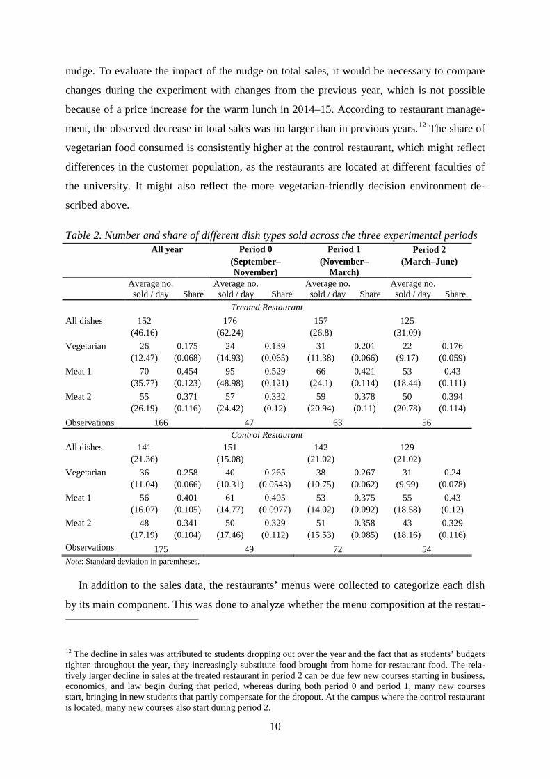
Descriptive statistics on the number of dishes sold overall and by dish type are shown in
Table 2. The treated restaurant is slightly bigger than the control restaurant, selling on average
152 warm lunches a day throughout the year, while the control sells on average about 140
dishes. Total sales decrease at both restaurants throughout the year. The decrease is larger at
the treated than at the control restaurant, which could be an unintended side effect of the 9 The cash registers have three different buttons that were labeled with the Swedish category names of the dishes, dagens husman (meat 1), gränslöst gott (meat 2), and grönt och gott (vegetarian), minimizing the risk of mis-takes in recording the type of dish correctly. An example picture of the registers is available on request. 10 The number of days differs because two job fairs took place at the treated restaurant building, during which the restaurant was closed. 11 During those days, which preceded public holidays, the control restaurant served only two warm dishes.
10
nudge. To evaluate the impact of the nudge on total sales, it would be necessary to compare
changes during the experiment with changes from the previous year, which is not possible
because of a price increase for the warm lunch in 2014–15. According to restaurant manage-
ment, the observed decrease in total sales was no larger than in previous years.12 The share of
vegetarian food consumed is consistently higher at the control restaurant, which might reflect
differences in the customer population, as the restaurants are located at different faculties of
the university. It might also reflect the more vegetarian-friendly decision environment de-
scribed above.
Table 2. Number and share of different dish types sold across the three experimental periods All year Period 0 Period 1 Period 2
(September–November)
(November–March)
(March–June)
Average no. sold / day Share
Average no. sold / day Share
Average no. sold / day Share
Average no. sold / day Share
Treated Restaurant All dishes 152
176
157
125
(46.16)
(62.24)
(26.8)
(31.09) Vegetarian 26 0.175 24 0.139 31 0.201 22 0.176
(12.47) (0.068) (14.93) (0.065) (11.38) (0.066) (9.17) (0.059)
Meat 1 70 0.454 95 0.529 66 0.421 53 0.43
(35.77) (0.123) (48.98) (0.121) (24.1) (0.114) (18.44) (0.111)
Meat 2 55 0.371 57 0.332 59 0.378 50 0.394
(26.19) (0.116) (24.42) (0.12) (20.94) (0.11) (20.78) (0.114)
Observations 166 47 63 56 Control Restaurant
All dishes 141
151
142
129
(21.36)
(15.08)
(21.02)
(21.02)
Vegetarian 36 0.258 40 0.265 38 0.267 31 0.24
(11.04) (0.066) (10.31) (0.0543) (10.75) (0.062) (9.99) (0.078)
Meat 1 56 0.401 61 0.405 53 0.375 55 0.43
(16.07) (0.105) (14.77) (0.0977) (14.02) (0.092) (18.58) (0.12)
Meat 2 48 0.341 50 0.329 51 0.358 43 0.329
(17.19) (0.104) (17.46) (0.112) (15.53) (0.085) (18.16) (0.116)
Observations 175 49 72 54 Note: Standard deviation in parentheses.
In addition to the sales data, the restaurants’ menus were collected to categorize each dish
by its main component. This was done to analyze whether the menu composition at the restau- 12 The decline in sales was attributed to students dropping out over the year and the fact that as students’ budgets tighten throughout the year, they increasingly substitute food brought from home for restaurant food. The rela-tively larger decline in sales at the treated restaurant in period 2 can be due few new courses starting in business, economics, and law begin during that period, whereas during both period 0 and period 1, many new courses start, bringing in new students that partly compensate for the dropout. At the campus where the control restaurant is located, many new courses also start during period 2.

11
rants changed over time and to control for different dish types in the empirical analysis. Meat
dishes were categorized by type of meat: beef, chicken, pork, other meat (minced meat, sau-
sages, game, lamb), and fish. An additional category was introduced for a soup that was
served as the meat 1 dish on 35 days (30 at the treated and 5 at the control restaurant), as it
could be customized to be vegetarian by omitting the bacon, without this being noticed by the
cashier who recorded the alternatives (meat 1, meat 2, or vegetarian).13 This soup is a tradi-
tional dish served on Thursdays throughout Sweden. The vegetarian dishes were categorized
partly according to components included and partly by type of dish, resulting in the categories
stew (such as a vegetarian curry), pasta, vegetables (for example, a vegetable gratin), patty
(for example, a vegetarian burger), other vegetarian (for example, pies or omelets), vegetarian
soup,14 and world (such as vegetarian enchiladas, Asian noodles, and falafel). For some types
of dishes, how often they occurred on the menu varied considerably. For example, vegetarian
dishes belonging to the patty category were offered on 11 percent and 13 percent of all days
during periods 0 and 1, respectively, but on 27 percent of all days during period 2. Appendix
Table A.1 shows how the restaurants’ menu compositions changed across experimental peri-
ods for both the vegetarian and the meat dishes.
Figure 1 shows that vegetarian dishes vary in popularity depending on the dish type. For
example, during the pre-experimental period, sales shares ranged from 12 percent for vegeta-
ble dishes to 21 percent for world dishes at the treated restaurant. The popularity pattern of
dishes looks similar across restaurants, with patties and world dishes being most popular.
13 As the soup could be customized to being vegetarian, the menu effectively contained two vegetarian and two meat dishes on the days it was served. This potentially creates measurement error in the share of vegetarian dish-es sold. To minimize the impact of potential measurement error in the regressions, the soup was classified as its own category of meat dishes and entered as a control variable in the main regression specifications. Empirical results are robust to excluding the days where soup was served and are available on request. 14 The vegetarian soup could also be customized to nonvegetarian by adding bacon, without this being noticed by the cashier. However, as it was served as the vegetarian dish, the menu effectively contained three meat dishes and one vegetarian dish on the days it was offered (12 days at the treated restaurant, 5 days at the control restau-rant). Again, the share of vegetarian dishes sold as the variable of interest is most likely subject to measurement error on those days. Controlling for the type of dish should ameliorate the measurement error.

12
Figure 1. Share of vegetarian dishes sold by type of dish
Note: Error bars represent 0.95 confidence intervals around the mean for each type. Error bar for soup in period 2 is omitted, as there was only one observation this period.
2.3. Empirical strategy
2.3.1. Before-after analysis
Building on the experimental design, two identification strategies are used to estimate the
effect of the nudge and its subsequent removal on the share of vegetarian dishes sold. The first
approach is to compare the sales share at the treated restaurant across periods, controlling for
additional factors:

13
𝑉𝑉𝑡𝑡 = 𝛼𝛼1 + 𝛾𝛾1𝑃𝑃𝑃𝑃𝑃𝑃𝑃𝑃𝑃𝑃𝑃𝑃1 + 𝛾𝛾2𝑃𝑃𝑃𝑃𝑃𝑃𝑃𝑃𝑃𝑃𝑃𝑃2 + 𝑉𝑉𝑃𝑃𝑉𝑉𝑉𝑉𝑉𝑉𝑉𝑉𝑃𝑃𝑡𝑡 × 𝜃𝜃 + (𝑀𝑀𝑃𝑃𝑀𝑀𝑉𝑉𝑉𝑉𝑉𝑉𝑉𝑉𝑃𝑃1𝑡𝑡 × 𝑀𝑀𝑃𝑃𝑀𝑀𝑉𝑉𝑉𝑉𝑉𝑉𝑉𝑉𝑃𝑃2𝑡𝑡) × 𝜇𝜇 +
𝜆𝜆𝑑𝑑𝑑𝑑𝑑𝑑 + 𝜀𝜀𝑡𝑡 (1)
𝑉𝑉𝑡𝑡 is the share of vegetarian lunches sold at restaurant 1 on day 𝑉𝑉. 𝑃𝑃𝑃𝑃𝑃𝑃𝑃𝑃𝑃𝑃𝑃𝑃1 and
𝑃𝑃𝑃𝑃𝑃𝑃𝑃𝑃𝑃𝑃𝑃𝑃2 are dummy variables indicating whether an observation belongs to the treatment or
the reversal period, respectively; 𝛾𝛾1 captures the effects of the combined nudge in period 1;
and 𝛾𝛾2 captures any remaining effects of the nudge after its removal in period 2.
𝑉𝑉𝑃𝑃𝑉𝑉𝑉𝑉𝑉𝑉𝑉𝑉𝑃𝑃𝑡𝑡 is a vector of dummy variables characterizing the type of vegetarian dish served
that day and is introduced to capture differences in popularity between dish types.
𝑀𝑀𝑃𝑃𝑀𝑀𝑉𝑉𝑉𝑉𝑉𝑉𝑉𝑉𝑃𝑃1𝑡𝑡 × 𝑀𝑀𝑃𝑃𝑀𝑀𝑉𝑉𝑉𝑉𝑉𝑉𝑉𝑉𝑃𝑃2𝑡𝑡 is a vector of all observed combinations of meat dishes of-
fered.15 It is introduced to control for the influence of the outside options on 𝑉𝑉𝑡𝑡. 𝜆𝜆𝑑𝑑𝑑𝑑𝑑𝑑 intro-
duces day-of-the-week fixed effects. To estimate how the nudge affects the sales of the meat 1
and meat 2 dishes, equation (1) can also be specified with the share of meat 1 or meat 2 dishes
sold as the dependent variable. While the intervention directly affected the visibility and menu
position of the meat 1 dish such that one would expect the sales share to decrease, sales of the
meat 2 dish could be also affected. Although the menu position and visibility of this dish were
kept constant throughout the experiment, the nudge might change its salience relative to the
meat 1 and vegetarian dishes.
The impact of the nudge over time can be analyzed by estimating equation (1) with a linear
time trend and by dividing the period dummies further into subperiods and comparing their
coefficients. This can also help elucidate whether the change of chefs at the treated restaurant
had an additional impact on the share of vegetarian dishes sold.
An alternative to looking separately at the share of each dish type sold as the dependent
variable in a linear regression framework is to model the sales of all three dish types, vegetar-
ian, meat 1, and meat 2, in a multinomial regression. This can serve as a robustness check for
the ordinary least squares (OLS) results, taking into account that the share of vegetarian dish-
es sold results from customers facing three unordered options they can choose from, and has
the advantage of simultaneously estimating the effect of the nudge on all three alternatives. I
estimate the following conditional logit model with alternative-specific constants, modelling
the probability 𝑉𝑉𝑡𝑡𝑡𝑡 that alternative 𝑗𝑗 is chosen at day 𝑉𝑉:
15 Alternatively, one could introduce each dish type separately in the regression. However, as the consumer is always faced with a combination of dishes, and the order in which they are presented on the menu might matter for decision-making, I control for each combination of meat types occurring in the data.

14
𝑉𝑉𝑡𝑡𝑡𝑡 = 𝑃𝑃𝑃𝑃𝑃𝑃𝑃𝑃[𝑌𝑌𝑡𝑡 = 𝑗𝑗] = 𝑒𝑒𝑒𝑒𝑒𝑒�𝛼𝛼𝑗𝑗+𝐷𝐷𝐷𝐷𝐷𝐷ℎ𝑡𝑡𝑑𝑑𝑒𝑒𝑒𝑒𝑡𝑡𝑗𝑗×𝜌𝜌+𝛾𝛾1𝑗𝑗𝑃𝑃𝑒𝑒𝑃𝑃𝐷𝐷𝑃𝑃𝑑𝑑1+𝛾𝛾2𝑗𝑗𝑃𝑃𝑒𝑒𝑃𝑃𝐷𝐷𝑃𝑃𝑑𝑑2+𝜆𝜆𝑗𝑗,𝐷𝐷𝐷𝐷𝐷𝐷�∑ 𝑒𝑒𝑒𝑒𝑒𝑒3𝑘𝑘=1 �𝛼𝛼𝑘𝑘+𝐷𝐷𝐷𝐷𝐷𝐷ℎ𝑡𝑡𝑑𝑑𝑒𝑒𝑒𝑒𝑡𝑡𝑘𝑘×𝜌𝜌+𝛾𝛾1𝑘𝑘𝑃𝑃𝑒𝑒𝑃𝑃𝐷𝐷𝑃𝑃𝑑𝑑1+𝛾𝛾2𝑘𝑘𝑃𝑃𝑒𝑒𝑃𝑃𝐷𝐷𝑃𝑃𝑑𝑑2+𝜆𝜆𝑘𝑘,𝐷𝐷𝐷𝐷𝐷𝐷�
(2)
where 𝑗𝑗,𝑘𝑘 = 1, 2, 3 denote the three alternatives (meat 1, meat 2, and vegetarian). Identifi-
cation in the conditional logit model crucially depends on the assumption of independence of
irrelevant alternatives (IIA), which excludes the presence of close substitute alternatives. As
the meat 1 and meat 2 dishes are very similar, it is likely that consumers eating meat substi-
tute between those two dishes to a greater extent than with the vegetarian dish. To relax the
IIA assumption, I also estimate a partially degenerate nested logit model that partitions the
choice set into one branch containing the meat alternatives and one branch containing the
vegetarian alternative (see, for example, Hunt, 2000).
Estimating effects of the nudge on the share of vegetarian dishes sold by before-after anal-
ysis will give unbiased results only if factors external to the experiment that might drive
changes in sales across the period can be excluded. Such external factors could, for example,
be food trends, media reporting on food-related issues, or seasonal variation in consumption
patterns. Given the long observation period, identification is especially sensitive to this (un-
testable) assumption. However, it can be relaxed by using data from restaurant 2 as a control,
which should capture any exogenous changes that could affect the consumption of vegetarian
food during the experiment, in a difference-in-differences analysis.
2.3.2 Difference-in-differences analysis
The following difference-in-differences (DiD) model is estimated to identify the effect of
the nudge on the share of vegetarian dishes sold by comparing changes across periods 0 and 1
at the treated restaurant with changes at the control restaurant:
𝑉𝑉𝐷𝐷𝑡𝑡 = 𝛼𝛼0 + 𝛽𝛽0𝑅𝑅𝑃𝑃𝑠𝑠𝑉𝑉𝑀𝑀𝑡𝑡𝑃𝑃𝑀𝑀𝑡𝑡𝑉𝑉 + 𝛾𝛾0𝑃𝑃𝑃𝑃𝑃𝑃𝑃𝑃𝑃𝑃𝑃𝑃1 + 𝛿𝛿0(𝑅𝑅𝑃𝑃𝑠𝑠𝑉𝑉𝑀𝑀𝑡𝑡𝑃𝑃𝑀𝑀𝑡𝑡𝑉𝑉 × 𝑃𝑃𝑃𝑃𝑃𝑃𝑃𝑃𝑃𝑃𝑃𝑃1) + 𝑉𝑉𝑃𝑃𝑉𝑉𝑉𝑉𝑉𝑉𝑉𝑉𝑃𝑃𝐷𝐷𝑡𝑡 × 𝜌𝜌 +
(𝑀𝑀𝑃𝑃𝑀𝑀𝑉𝑉𝑉𝑉𝑉𝑉𝑉𝑉𝑃𝑃1𝐷𝐷𝑡𝑡 × 𝑀𝑀𝑃𝑃𝑀𝑀𝑉𝑉𝑉𝑉𝑉𝑉𝑉𝑉𝑃𝑃2𝐷𝐷𝑡𝑡) × 𝜏𝜏 + 𝜆𝜆𝐷𝐷𝑑𝑑𝑑𝑑 + 𝜆𝜆𝐻𝐻𝑃𝑃𝐻𝐻𝐷𝐷𝑑𝑑𝑑𝑑𝑑𝑑𝐷𝐷 + 𝜆𝜆𝑀𝑀𝑃𝑃𝑀𝑀𝑡𝑡ℎ + 𝜀𝜀𝐷𝐷𝑡𝑡 (3)
where 𝑉𝑉𝐷𝐷𝑡𝑡 is the share of vegetarian lunch dishes sold at restaurant 𝑃𝑃 on day 𝑉𝑉. Initial differ-
ences in the share of vegetarian lunches sold are captured by the dummy variable
𝑅𝑅𝑃𝑃𝑠𝑠𝑉𝑉𝑀𝑀𝑡𝑡𝑃𝑃𝑀𝑀𝑡𝑡𝑉𝑉, which is 0 for the control restaurant and 1 for the treated restaurant. 𝑃𝑃𝑃𝑃𝑃𝑃𝑃𝑃𝑃𝑃𝑃𝑃1 is
a dummy variable taking the value 1 if an observation belongs to the treatment period and
controls for changes in the popularity of vegetarian food across periods common to both res-
taurants. 𝑉𝑉𝑃𝑃𝑉𝑉𝑉𝑉𝑉𝑉𝑉𝑉𝑃𝑃𝐷𝐷𝑡𝑡 is again a vector of dummy variables characterizing the type of vegetari-
an dish served, and 𝑀𝑀𝑃𝑃𝑀𝑀𝑉𝑉𝑉𝑉𝑉𝑉𝑉𝑉𝑃𝑃1𝐷𝐷𝑡𝑡 × 𝑀𝑀𝑃𝑃𝑀𝑀𝑉𝑉𝑉𝑉𝑉𝑉𝑉𝑉𝑃𝑃2𝐷𝐷𝑡𝑡 controls for the combination of meat dishes
served as outside options. 𝜆𝜆𝐷𝐷𝑑𝑑𝑑𝑑,𝜆𝜆𝐻𝐻𝑃𝑃𝐻𝐻𝐷𝐷𝑑𝑑𝑑𝑑𝑑𝑑, and 𝜆𝜆𝑀𝑀𝑃𝑃𝑀𝑀𝑡𝑡ℎ are time fixed effects controlling for the

15
day of the week, for the weeks around the Christmas holidays16, and for the calendar month.
Month fixed effects are especially important, as they capture any potential common effects of
the chef change in February on the outcome variable. 𝑅𝑅𝑃𝑃𝑠𝑠𝑉𝑉𝑀𝑀𝑡𝑡𝑃𝑃𝑀𝑀𝑡𝑡𝑉𝑉 × 𝑃𝑃𝑃𝑃𝑃𝑃𝑃𝑃𝑃𝑃𝑃𝑃1 indicates
whether an observation belongs to the treated restaurant in the treatment period, and 𝛿𝛿0 cap-
tures the treatment effect.
DiD estimation is limited to the direct effect of the nudge (i.e., the effect in period 1), as it
relies on two critical assumptions to deliver unbiased treatment effects. The first assumption
is that the consumption of vegetarian food followed parallel trends at both restaurants before
the introduction of the nudge. The second assumption is that restaurant 2 is a valid control in
the sense that any exogenous events during the experiment affected consumers at both restau-
rants in a similar way. This assumption is weakened by the employment of a new chef toward
the end of the treatment period at the control restaurant. Figure 2, which depicts weekly aver-
age sales of vegetarian dishes by restaurant, shows that from the week the new chef started,
variability increased and sales shares slightly decreased at the control restaurant.17 According
to the restaurant’s management, the higher variability in the share of vegetarian dishes sold
was due to the fact that the new chef was not used to cooking vegetarian dishes and first had
to acquire knowledge regarding the taste of his customers. Moreover, the menu order was
changed for five weeks during the reversal period, such that the vegetarian dish was moved
from the top to the middle of the menu. The change of chefs at restaurant 1 did not lead to a
similar increase in variability, which is most likely because the new chef had worked there
before as a trainee of the old chef. Hence, he already knew the taste of the customers and was
familiar with cooking vegetarian dishes. Limiting the DiD analysis to period 1 safeguards
against overestimating persistent effects of the nudge in period 2. In addition, equation (3) is
estimated with period 1 divided further into subperiods and with a linear time trend, which
can provide some information about the impact of the chef change on the treatment effect.
Figure 2 can also be used to examine the parallel trends assumption. A priori, this assump-
tion is supported by several factors. Both restaurants are run by the same provider and subject
to the same management, which minimizes the chance for management changes that affect
only one restaurant. Moreover, both restaurants are located in the same city, and customers
16 Potentially, more employees take holidays during these weeks, which could alter the customer composition. 17 The spike in the last week of March coincides with the week before the Easter holidays, when the restaurant was open for only three days. This could have altered the composition of customers. Most likely, both the lower number of observations and the composition effect contributed to the spike in the share of vegetarian dishes sold. The treated restaurant was open for four days that week.

16
should be exposed to roughly the same media, weather conditions, and seasonal variation in
food offered. Third, although the restaurants differ with respect to the customers to whom
they cater, as they belong to different faculties, the populations are similar with respect to age
structure and educational attainment, increasing the likelihood that they will react to exoge-
nous events in a similar way.
Figure 2. Share of vegetarian meals sold per week over time, both restaurants
Examining pretreatment trends in Figure 2 lends support to the assumption of parallel
trends during the baseline period. At the control restaurant, the share of vegetarian dishes sold
did not trend upward or downward until the new chef was employed. The apparent spike at
the start of the intervention was most likely caused by the type of vegetarian dishes offered,
which was a dish belonging to the most popular category (patties) during three out of five
days. At the treated restaurant, the share of vegetarian dishes sold exhibits more variation but
no clear trend during the preintervention period, and it increased steadily after the implemen-
tation of the nudge. The drop exactly at the start of the intervention was most likely caused by
the fact that a job fair was taking place at the treated restaurant; only one day of sales data was
delivered during that week. On that day, a vegetarian dish belonging to one of the least popu-
lar categories, stew, was sold. During the reversal period, the share of vegetarian lunches at
the treated restaurant dropped compared with the intervention period but was still slightly
higher than during the baseline period.

17
In addition to using a linear DiD model, sales in period 1 are also modelled by a condition-
al logit model and a nested model to relax the IIA assumption. The conditional logit model
takes the following form, where pitj denotes the probability that alternative j is chosen in res-
taurant 𝑃𝑃 at day 𝑉𝑉, and R and P1 are dummies for restaurant 1 and period 1, respectively:
𝑉𝑉𝑡𝑡𝑡𝑡 = 𝑃𝑃𝑃𝑃𝑃𝑃𝑃𝑃[𝑌𝑌𝑡𝑡𝐷𝐷 = 𝑗𝑗] = 𝑒𝑒𝑒𝑒𝑒𝑒�𝛼𝛼𝑗𝑗+𝛽𝛽𝑗𝑗𝑅𝑅+𝛾𝛾𝑗𝑗𝑃𝑃1+𝛿𝛿𝑗𝑗(𝑅𝑅×𝑃𝑃1)+𝐷𝐷𝐷𝐷𝐷𝐷ℎ𝑡𝑡𝑑𝑑𝑒𝑒𝑒𝑒𝑖𝑖𝑡𝑡𝑗𝑗×𝜌𝜌+𝜆𝜆𝑗𝑗,𝐷𝐷𝐷𝐷𝐷𝐷+𝜆𝜆𝑗𝑗,𝐻𝐻𝐻𝐻𝐻𝐻𝑖𝑖𝐻𝐻+𝜆𝜆𝑗𝑗,𝑀𝑀𝐻𝐻𝑀𝑀𝑡𝑡ℎ�∑ 𝑒𝑒𝑒𝑒𝑒𝑒3𝑘𝑘=1 �𝛼𝛼𝑘𝑘+𝛽𝛽𝑘𝑘𝑅𝑅+𝛾𝛾𝑘𝑘𝑃𝑃1+𝛿𝛿𝑘𝑘(𝑅𝑅×𝑃𝑃1)+𝐷𝐷𝐷𝐷𝐷𝐷ℎ𝑡𝑡𝑑𝑑𝑒𝑒𝑒𝑒𝑖𝑖𝑡𝑡𝑘𝑘×𝜌𝜌+𝜆𝜆𝑘𝑘,𝐷𝐷𝐷𝐷𝐷𝐷+𝜆𝜆𝑘𝑘,𝐻𝐻𝐻𝐻𝐻𝐻𝑖𝑖𝐻𝐻+𝜆𝜆𝑘𝑘,𝑀𝑀𝐻𝐻𝑀𝑀𝑡𝑡ℎ�
(4)
3. Results
3.1. Preliminary analysis
Table 2 compares the average shares of vegetarian dishes sold across periods and restau-
rants. At the treated restaurant, the share significantly increased by 6 percentage points, from
14 to 20 percent, after implementing the nudge, while it remained stable at around 26 percent
at the control restaurant. Comparing the changes in the share of vegetarian dishes sold at the
treated restaurant between period 0 and period 1 to changes in sales share at the control res-
taurant across the same periods provides the unconditional DiD treatment effect. Without con-
trolling for additional factors, the share of vegetarian dishes sold at the treated restaurant in-
creased by 6 percentage points (column (4)). In period 2, the share of vegetarian lunches sold
dropped to around 18 percent and 24 percent at the treated and control restaurants, respective-
ly. Comparing the shares in period 0 and period 2 at the treated restaurant shows that the sales
share of vegetarian lunches was still 3.6 percentage points higher after the nudge was re-
moved than during the baseline period. The DiD estimate is significantly higher but most like-
ly confounded by the drop in sales shares in connection with the employment of the new chef
at the control restaurant.
Table 3. Mean shares of vegetarian dishes sold across periods and restaurants (1) (2) (3) (4) (5) (6) Share of vegetarian dishes sold Period 0 Period 1 Period 2 Period 1–
Period 0a Period 2–Period 0a
Period 2–Period 1a
Treated restaurant 0.139 (0.0038)
0.201 (0.0040)
0.176 (0.0046)
0.062*** (0.0055)
0.036*** (0.0059)
–0.025*** (.0060)
Control restaurant 0.264 (0.0051)
0.267 (0.0044)
0.240 (0.0051)
–0.003 (0.0067)
–0.025*** (.0072)
–0.026*** (0.0067)
Difference-in-differences treated – controlb
0.060*** (0.0166)
0.061*** (0.0180)
0.001 (0.0170)
a z-test of proportions b regression t-test Standard errors in parentheses, *** p < 0.01, ** p < 0.05, * p < 0.1

18
3.2. Regression analysis: Immediate effects of the nudge
Table 4 presents the estimated effects of the nudge in period 1, using the before-after ap-
proach in columns (1) – (4) and the DiD approach in columns (5) – (8). Column 1 shows the
raw before-after comparison; the share of vegetarian dishes sold significantly increases by 6.2
percentage points. Columns (2) and (3) add controls for the types of vegetarian and meat
dishes sold each day. Although appendix Table A.1 shows that the menu composition varied
across periods, controlling for it only marginally changes the treatment effect—to 6.4 per-
centage points when including the type of vegetarian dish and to 7.2 percentage points when
including the types of meat dishes. Including weekday fixed effects (column (4)) increases the
treatment effect further to 8.2 percentage points. Testing for pairwise differences reveals that
treatment effects are not significantly different across specifications. Columns (5) – (8) show
the results of the DiD estimation. DiD estimates of the treatment effect lie between 6 and 7.3
percentage points and are thus very close to the before-after estimates. Pairwise comparisons
show no difference in the treatment effects across models. A minimum treatment effect of 6
percentage points, as found in the specification in column (5), represents a 43 percent increase
in the share of vegetarian lunches sold, compared with the baseline period, as the result of the
nudge.

19
Tabl
e 4.
Est
imat
ing
the
imm
edia
te e
ffect
s of t
he n
udge
on
the
shar
e of
veg
etar
ian
dish
es so
ld
B
efor
e-af
ter e
stim
atio
n D
iffer
ence
-in-d
iffer
ence
s est
imat
ion
Dep
ende
nt v
aria
ble:
Sha
re o
f ve
geta
rian
dish
es/d
ay
(1)
No
cont
rols
(2
) +
Type
of
vege
taria
n di
sh
(3)
+ Ty
pe o
f m
eat d
ish
(4)
+ D
ay-o
f-w
eek
FE
(5)
No
cont
rols
(6
) +
Type
of v
ege-
taria
n di
sh
(7)
+ Ty
pe o
f mea
t di
sh
(8)
+ Ti
me
FE
Perio
d 1
0.06
17**
* 0.
0642
***
0.07
23**
* 0.
0820
***
0.00
130
0.00
0503
0.
0012
0 –0
.014
9
(0.0
126)
(0
.011
5)
(0.0
108)
(0
.012
1)
(0.0
115)
(0
.010
8)
(0.0
116)
(0
.024
3)
Trea
ted
rest
aura
nt
–0.1
26**
* –0
.125
***
–0.1
34**
* –0
.138
***
0.
0013
0 0.
0005
03
0.00
120
(0.0
134)
Pe
riod
1 ×
Trea
ted
rest
aura
nt
0.06
04**
* 0.
0627
***
0.06
99**
* 0.
0730
***
(0
.016
6)
(0.0
156)
(0
.016
2)
(0.0
166)
C
onst
ant
0.13
9***
0.
124*
**
0.13
6***
0.
138*
**
0.26
5***
0.
248*
**
0.28
2***
0.
320*
**
(0
.009
56)
(0.0
153)
(0
.023
1)
(0.0
393)
(0
.008
87)
(0.0
112)
(0
.022
1)
(0.0
353)
Obs
erva
tions
11
0 11
0 11
0 11
0 23
1 23
1 23
1 23
1 A
djus
ted
R-sq
uare
d 0.
173
0.32
8 0.
452
0.43
3 0.
393
0.47
9 0.
522
0.52
6 V
egty
pe
No
Yes
Y
es
Yes
N
o Y
es
Yes
Y
es
Mea
ttype
N
o N
o Y
es
Yes
N
o N
o Y
es
Yes
M
onth
FE
No
No
No
No
No
No
No
Yes
H
olid
ay F
E N
o N
o N
o N
o N
o N
o N
o Y
es
Wee
kday
FE
No
No
No
Yes
N
o N
o N
o Y
es
Not
e: C
onve
ntio
nal s
tand
ard
erro
rs a
re u
sed,
as t
he re
sidu
als e
xhib
it ve
ry li
ttle
hete
rosc
edas
ticity
and
as t
hey
prov
ide
the
mos
t con
serv
ativ
e co
nfid
ence
inte
rval
s in
all s
peci
ficat
ions
, eve
n w
hen
com
pare
d w
ith b
ias-
corr
ecte
d ro
bust
stan
dard
err
ors.
See
Ang
rist a
nd P
isch
ke (2
008)
. St
anda
rd e
rror
s in
pare
nthe
ses,
***
p <
0.01
, **
p <
0.05
, * p
< 0
.1.

20
To analyze the development of the treatment effect over time, the intervention period is
split into three subperiods: November–December, January, and February–March.18 Results in
columns (1) and (4) of Table 5 confirm the graphical analysis: the size of the treatment effect
increases over time, from 4.1 to 11.3 percentage points when estimated by a before-after
comparison, and from (insignificant) 1.2 to 13.5 percentage points when estimated by DiD.19
The effect for February–March is most likely slightly overestimated in the DiD specification,
as these are the months when the new chef was employed and the share of vegetarian dishes
dropped slightly at the control restaurant (see Figure 2). However, the effect for February–
March does not differ significantly between the before-after and the DiD specification.20
Estimating the treatment effect with a linear time trend (columns (2), (3), and (5)) shows
that the nudge led to an increase of 0.8–0.9 percentage points in the share of vegetarian dishes
sold each week. In column (2), a weekly linear trend is estimated using only data from the
treated restaurant up to February 1, when the new chef started. Column (3) estimates the trend
using all of period 1 but includes a dummy for the period February–March. The trend slightly
decreases but is not significantly different from using only the data up to the chef change (p =
0.10), providing evidence that the change of chefs at the treated restaurant did not significant-
ly change the impact of the nudge. Excluding the first week of the intervention, which repre-
sents a potential outlier at both restaurants (see Figure 2), as a robustness check for the linear
time trend decreases the weekly trend to 0.75–0.84 percentage points, depending on the speci-
fication used.21
As individual-level data is not available, it is impossible to identify the mechanism behind
the increasing treatment effect. One potential explanation is that an increasing number of in-
dividuals were exposed to the nudge over the course of the intervention. A guest survey con-
ducted in May 2015 revealed that on average, customers eat at the restaurant about four times
per month. If initially nudged customers subsequently increased their consumption of vegetar-
ian food further, such as predicted by the models of Becker and Murphy (1988) or Naik and
Moore (1996), this could result in an increasing treatment effect over time. Another explana- 18 November and December were grouped because only about half of November was treated and the Christmas break started December 19. February and March were grouped because only one week in March was treated. 19 In model (1), pairwise comparison of treatment effects shows that the effects for January and February–March are not significantly different from each other. Both other pairwise comparisons show significant differences. In model (4), all pairwise comparisons show that monthly, the treatment effect increases over time. 20 Treatment effects for November–December are significantly different at a 5% level in both the before-after and the DiD specifications. Effects for January and February–March are not significantly different (p = 0.08 and p = 0.13, respectively). 21 Full results of the regressions excluding the first week of the intervention are available on request.

21
tion could be that any increase in the sales of vegetarian dishes as a result of the nudge in-
creased sales further via network effects, such as if people recommended the dish to col-
leagues or if customers observed what others chose. Such effects could lead to increasing
sales over time, even if the additional sales might not be directly attributable to the nudge.
Table 5. Treatment effects over time Before-after estimation DiD estimation (1) (2) (3) (4) (5) Monthly
treatment effects
Linear time trend, be-fore chef change
Linear time trend, whole
period
Monthly treatment
effects
Linear time trend
Period 1 0.00788 (0.0215) Restaurant 1 -0.142*** -0.146*** (0.0125) (0.0111) Period 1 × Restaurant 1 Nov–Dec × Restaurant 1 0.0407*** 0.0115 (0.0142) (0.0197) Jan × Restaurant 1 0.0968*** 0.0733*** (0.0159) (0.0228) Feb–Mar × Restaurant 1 0.113*** 0.135*** (0.0146) (0.0199) Weekly trend × Period 1 × 0.0090*** 0.0083*** 0.0085*** Restaurant 1 (0.0014) (0.0014) (0.0012) Constant 0.152*** 0.158*** 0.162*** 0.319*** 0.304*** (0.0353) (0.0347) (0.0350) (0.0337) (0.0328) Observations 110 87 110 231 231 Adjusted R-squared 0.547 0.521 0.539 0.591 0.587 Vegtype Yes Yes Yes Yes Yes Meattype New chef
Yes No
Yes No
Yes Yes
Yes No
Yes No
Month FE No No No Yes Yes Holiday FE No No No Yes Yes Weekday FE Yes Yes Yes Yes Yes Note: The baseline specifications shown in columns (1) and (4) correspond with columns (4) and (8) in Table 4. Standard errors in parentheses, *** p < 0.01, ** p < 0.05, * p < 0.1.
3.3. Persistent effects of the nudge on the share of vegetarian dishes sold
Table 6 shows the results of the before-after regressions testing for persistent changes in
the share of vegetarian dishes sold after removing the nudge. When estimating the full model,
including controls for dish types and weekday fixed effects (column (4)), the share of vegetar-
ian lunches is still around 4 percentage points higher than in the baseline period. Combining
the results from the analysis of treatment effect over time and from the reversal of the inter-

22
vention, the nudge seems to have led to a persistent shift in consumption toward more vege-
tarian food.22
Table 6. Estimating persistent effects of the nudge on the share of vegetarian dishes sold Dependent variable: Share of vegetarian dishes sold per day
(1) No controls
(2) + Type of vege-
tarian dish
(3) + Type of meat
dish
(4) + Day-of-week
FE Period 1 0.0617*** 0.0642*** 0.0703*** 0.0703*** (0.0122) (0.0117) (0.0118) (0.0122) Period 2 0.0365*** 0.0367*** 0.0404*** 0.0409*** (0.0125) (0.0121) (0.0124) (0.0126) Constant 0.139*** 0.127*** 0.148*** 0.154*** (0.00922) (0.0136) (0.0279) (0.0315) Observations 166 166 166 166 Adjusted R-squared 0.125 0.209 0.286 0.268 Vegtype No Yes Yes Yes Meattype No No Yes Yes Month FE No No No No Holiday FE No No No No Weekday FE No No No Yes Note: Conventional standard errors are used as the residuals exhibit very little heteroscedasticity and as they provide the most conservative confidence intervals in all specifications, even when compared with bias-corrected robust standard errors. Standard errors in parentheses*** p < 0.01, ** p < 0.05, * p < 0.1.
3.4. Heterogeneous effects: Type of vegetarian dish served
As Figure 1 shows, the sales share of vegetarian dishes varied considerably with the type
of dish offered. This section analyzes whether the impact of the nudge varied across dish
types. Changing the visibility of the dish can be expected to have a differential impact, de-
pending on how appealing a dish looks and how this contrasts with the expectations formed
by the customers when only reading the name of a dish.
Figure 3 shows how the sales share of vegetarian dishes changed across periods for each
type of dish at the treated restaurant, according to the classification used in the regression
analysis. It can be seen that the intervention increased the sales of all vegetarian dish types,
but effects vary considerably across types. The nudge seems to work most effectively when a
vegetarian patty is sold and least effectively when a stew is sold. One explanation could be
that the appearance of patties, such as vegetarian burgers, appeals more to customers who
usually consume meat or fish, as they resemble typical meat dishes. This explanation is cor-
roborated by previous research finding that industry meat substitutes, such as soy burgers, are
22 There is no evidence for a decline in the share of vegetarian dishes sold during the reversal period. When the reversal period is divided into two parts (March–April and May–June), treatment effects are 0.044 and 0.036, respectively, and not significantly different from each other. Results for the split reversal period are available on request.

23
relatively popular meat substitutes for consumers adhering to flexible diets (i.e., those that are
neither vegetarians nor heavy meat eaters) (Schösler et al., 2012). Stews, on the other hand,
seem to attract only the core vegetarian customers even during the treatment condition, as
their share hardly increased while the nudge was implemented. However, although the effects
for patties and vegetables are large in absolute terms in period 1, none are statistically signifi-
cant when tested in a regression (see appendix Table A.2), which could be due to the relative-
ly low frequency with which each category was served.
Figure 3. Share of vegetarian dishes sold across periods, by type of vegetarian dish
Note: The short dashed lines represent the mean share of vegetarian dishes sold in period 0; long dashed lines, the mean share sold in period 1; and dotted lines, mean shares sold in period 2. Error bars represent 0.95 confidence intervals around the mean for each type.
3.5. Alternative model specifications and substitution effects
Although the nudge changed only how the vegetarian and meat 1 dishes were presented,
Figure 4 provides some indication that the sales share of the meat 2 dish was also affected by
the intervention. Plotting the sales shares of all three dish types shows that the meat 1 and
meat 2 dish were close substitutes, as their sales are highly negatively correlated (r = -0.84). It
also shows an increase in the unconditional sales share of the meat 2 dish (not controlling for
dish types or time effects) during period 1 and period 2 compared with the baseline period.

24
Figure 4. Development of sales shares of all three dish types over time, treated restaurant
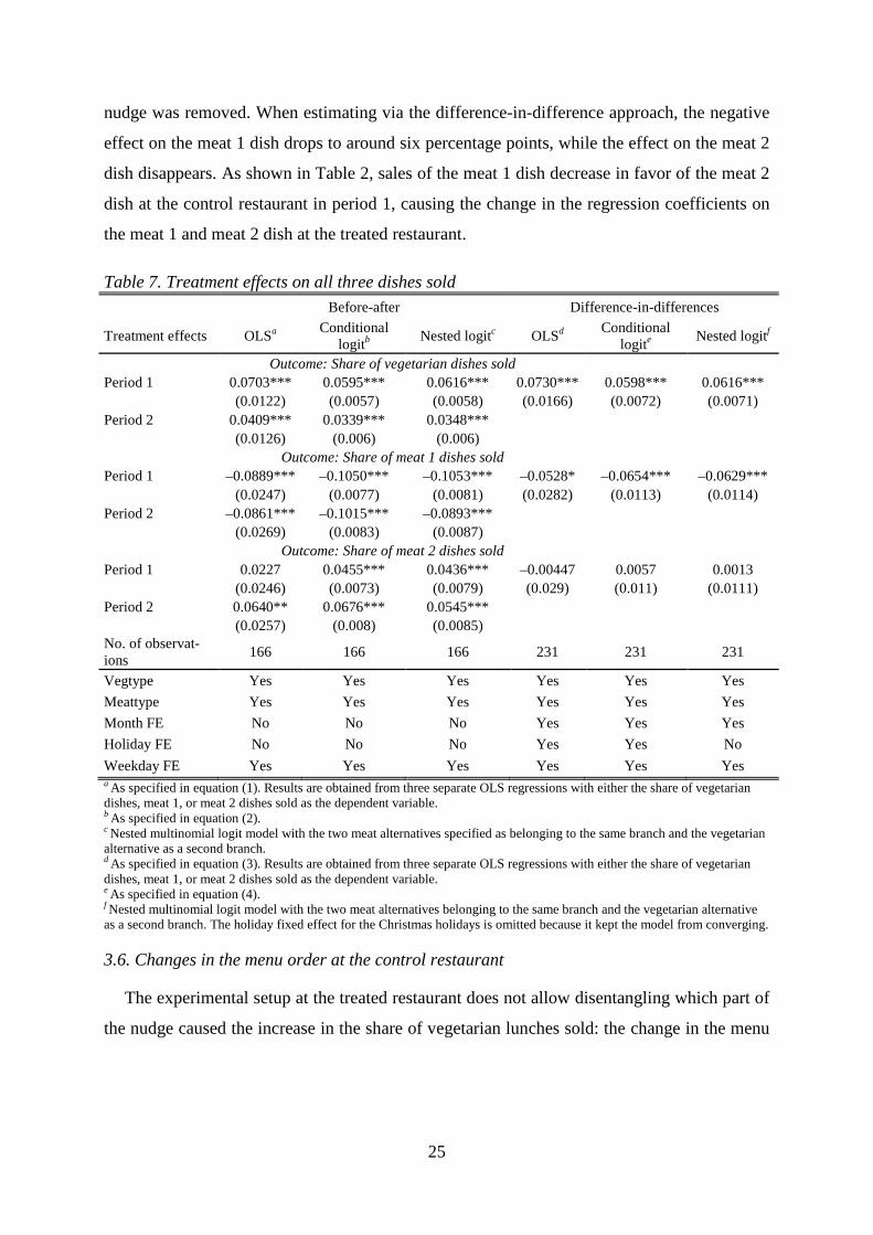
Regression results confirm the graphical analysis. Table 7 shows treatment effects on all
three dish types resulting from estimating OLS, conditional logit and nested logit regressions,
controlling for the type of meat or vegetarian food served and time. The coefficients shown
are the marginal effects of the treatment on the sales shares.23 Estimated treatment effects are
largely similar, showing that the OLS results are robust to alternative model specifications.
Results from the nested logit models, which are preferred over the conditional logit results
because they are not sensitive to the IIA assumption,24 show that the increase in the number
of vegetarian dishes sold was accompanied by a decrease in the meat 1 dish by around 10 per-
centage points and an increase in the meat 2 dish by around 4 percentage points in period 1 if
estimated using the before-after specification, and all effects persist into period 2 when the
23 Puhani (2012) shows that the treatment effect in nonlinear difference-in-differences models is given by the incremental effect of the treatment indicator on the outcome variable:
∆𝑃𝑃𝑃𝑃[𝑑𝑑𝑖𝑖𝑡𝑡=𝑡𝑡]∆𝑃𝑃𝑒𝑒𝑃𝑃𝐷𝐷𝑃𝑃𝑑𝑑1×𝑅𝑅𝑒𝑒𝐷𝐷𝑡𝑡1
=
𝑃𝑃𝑒𝑒𝑉𝑉�𝛼𝛼𝑗𝑗+𝛽𝛽𝑗𝑗𝑅𝑅+𝛾𝛾𝑗𝑗𝑃𝑃1+𝛿𝛿𝑗𝑗(𝑅𝑅×𝑃𝑃1)+𝐷𝐷𝑃𝑃𝑠𝑠ℎ𝑉𝑉𝑉𝑉𝑉𝑉𝑃𝑃𝑃𝑃𝑉𝑉𝑗𝑗
×𝜌𝜌+𝜆𝜆𝑗𝑗,𝐷𝐷𝑀𝑀𝑉𝑉+𝜆𝜆𝑗𝑗,𝐻𝐻𝑃𝑃𝐻𝐻𝑃𝑃𝑃𝑃+𝜆𝜆𝑗𝑗,𝑀𝑀𝑃𝑃𝑡𝑡𝑉𝑉ℎ�
∑ 𝑃𝑃𝑒𝑒𝑉𝑉3𝑘𝑘=1 �𝛼𝛼𝑘𝑘+𝛽𝛽𝑘𝑘𝑅𝑅1+𝛾𝛾𝑘𝑘𝑃𝑃1+𝛿𝛿𝑘𝑘(𝑅𝑅×𝑃𝑃1)+𝐷𝐷𝑃𝑃𝑠𝑠ℎ𝑉𝑉𝑉𝑉𝑉𝑉𝑃𝑃𝑃𝑃𝑉𝑉𝑘𝑘×𝜌𝜌+𝜆𝜆𝑘𝑘,𝐷𝐷𝑀𝑀𝑉𝑉+𝜆𝜆𝑘𝑘,𝐻𝐻𝑃𝑃𝐻𝐻𝑃𝑃𝑃𝑃+𝜆𝜆𝑘𝑘,𝑀𝑀𝑃𝑃𝑡𝑡𝑉𝑉ℎ�
−𝑃𝑃𝑒𝑒𝑉𝑉�𝛼𝛼𝑗𝑗+𝛽𝛽𝑗𝑗𝑅𝑅+𝛾𝛾𝑗𝑗𝑃𝑃1+𝐷𝐷𝑃𝑃𝑠𝑠ℎ𝑉𝑉𝑉𝑉𝑉𝑉𝑃𝑃
𝑃𝑃𝑉𝑉𝑗𝑗×𝜌𝜌+𝜆𝜆𝑗𝑗,𝐷𝐷𝑀𝑀𝑉𝑉+𝜆𝜆𝑗𝑗,𝐻𝐻𝑃𝑃𝐻𝐻𝑃𝑃𝑃𝑃+𝜆𝜆𝑗𝑗,𝑀𝑀𝑃𝑃𝑡𝑡𝑉𝑉ℎ�
∑ 𝑃𝑃𝑒𝑒𝑉𝑉3𝑘𝑘=1 �𝛼𝛼𝑘𝑘+𝛽𝛽𝑘𝑘𝑅𝑅+𝛾𝛾𝑘𝑘𝑃𝑃1+𝐷𝐷𝑃𝑃𝑠𝑠ℎ𝑉𝑉𝑉𝑉𝑉𝑉𝑃𝑃𝑃𝑃𝑉𝑉𝑘𝑘×𝜌𝜌+𝜆𝜆𝑘𝑘,𝐷𝐷𝑀𝑀𝑉𝑉+𝜆𝜆𝑘𝑘,𝐻𝐻𝑃𝑃𝐻𝐻𝑃𝑃𝑃𝑃+𝜆𝜆𝑘𝑘,𝑀𝑀𝑃𝑃𝑡𝑡𝑉𝑉ℎ�
,
where 𝑗𝑗, 𝑘𝑘 = 1, 2, 3 denote the three dish alternatives. The treatment effect is estimated as the marginal effect at data means. Standard errors are obtained by using the delta method. 24 A formal Hausman test of the IIA assumption did not provide valid results, as the covariance matrix for the difference between the restricted and unrestricted models was not positive definite. This is most likely a finite sample problem. As the IIA cannot be assumed to hold, and the nested logit model should be preferred.
25
nudge was removed. When estimating via the difference-in-difference approach, the negative
effect on the meat 1 dish drops to around six percentage points, while the effect on the meat 2
dish disappears. As shown in Table 2, sales of the meat 1 dish decrease in favor of the meat 2
dish at the control restaurant in period 1, causing the change in the regression coefficients on
the meat 1 and meat 2 dish at the treated restaurant.
Table 7. Treatment effects on all three dishes sold Before-after Difference-in-differences
Treatment effects OLSa Conditional logitb Nested logitc OLSd Conditional
logite Nested logitf
Outcome: Share of vegetarian dishes sold Period 1 0.0703*** 0.0595*** 0.0616*** 0.0730*** 0.0598*** 0.0616***
(0.0122) (0.0057) (0.0058) (0.0166) (0.0072) (0.0071) Period 2 0.0409*** 0.0339*** 0.0348***
(0.0126) (0.006) (0.006) Outcome: Share of meat 1 dishes sold Period 1 –0.0889*** –0.1050*** –0.1053*** –0.0528* –0.0654*** –0.0629***
(0.0247) (0.0077) (0.0081) (0.0282) (0.0113) (0.0114) Period 2 –0.0861*** –0.1015*** –0.0893***
(0.0269) (0.0083) (0.0087) Outcome: Share of meat 2 dishes sold Period 1 0.0227 0.0455*** 0.0436*** –0.00447 0.0057 0.0013
(0.0246) (0.0073) (0.0079) (0.029) (0.011) (0.0111) Period 2 0.0640** 0.0676*** 0.0545***
(0.0257) (0.008) (0.0085) No. of observat-
ions 166 166 166 231 231 231
Vegtype Yes Yes Yes Yes Yes Yes Meattype Yes Yes Yes Yes Yes Yes Month FE No No No Yes Yes Yes Holiday FE No No No Yes Yes No Weekday FE Yes Yes Yes Yes Yes Yes a As specified in equation (1). Results are obtained from three separate OLS regressions with either the share of vegetarian dishes, meat 1, or meat 2 dishes sold as the dependent variable. b As specified in equation (2). c Nested multinomial logit model with the two meat alternatives specified as belonging to the same branch and the vegetarian alternative as a second branch. d As specified in equation (3). Results are obtained from three separate OLS regressions with either the share of vegetarian dishes, meat 1, or meat 2 dishes sold as the dependent variable. e As specified in equation (4). f Nested multinomial logit model with the two meat alternatives belonging to the same branch and the vegetarian alternative as a second branch. The holiday fixed effect for the Christmas holidays is omitted because it kept the model from converging.
3.6. Changes in the menu order at the control restaurant
The experimental setup at the treated restaurant does not allow disentangling which part of
the nudge caused the increase in the share of vegetarian lunches sold: the change in the menu

26
order or the increased visibility of the vegetarian dish.25 Evidence that changing the menu
order in isolation play at least some role comes from the control restaurant. As mentioned
earlier, the new chef changed the menu order during five nonconsecutive weeks, resulting in
22 days with a changed order out of the 79 days in the sample when the new chef was em-
ployed. Despite the small sample, when regressing daily sales of all three dish types on a
dummy for changed menu order, type of meat or vegetarian dish, and weekday fixed effects in
a nested logit model, there is a significant negative effect of –2.4 percentage points from list-
ing the vegetarian dish in the middle instead of at the top (see Table 8). The effect of being
put at the top is larger; sales of the meat 1 dish increased by around 4 percentage points on the
days when the menu order was changed. The reduction in sales of the meat 2 dish is not sig-
nificant but still indicates that there was some substitution from the meat 2 to the meat 1 dish
when the latter was placed at the top.26 Analyzing the menu changes in the control restaurant
shows that it is possible not only to be nudged into switching to vegetarian food, but also to
be nudged away from it.
Table 8. Effects of the change in the menu order at the control restaurant Nested logit model Share of vegetarian
dishes sold Share of meat 1
dishes sold Share of meat 2
dishes sold Menu order changed –0.0237** 0.0380*** –0.0143 (0.0097) (0.0123) (0.0119) Observations 79 79 79 Vegtype Yes Yes Yes Meattype Yes Yes Yes Weekday FE Yes Yes Yes Note: Only observations when the new chef was employed were used ( 17 weeks of data), of which the menu order was changed during five weeks. Treatment effects are calculated as the incremental effect of the treatment indicator on the out-come variable (Puhani, 2012) and as marginal effects at data means. Standard errors are obtained by using the delta method. Standard errors in parentheses, *** p < 0.01, ** p < 0.05, * p < 0.1.
25 A priori, it seems more likely that it was the increased visibility that, via a change in saliency and additional information, caused most of the treatment effect. Order effects based on growing fatigue or satisficing behavior seem more apt to arise with longer lists, and previous studies included lists containing many more items than the menus in this study (for example, Dayan and Bar-Hillel, 2011; Feenberg et al., 2015; Policastro et al., 2015). Confirmatory bias, on the other hand, might cause a primacy effect even with such a short list. 26 The results of changing the menu order at the control restaurant are robust to excluding the outlier identified in Figure 2. Excluding that week changes the effect on the vegetarian dish to –0.0216 but leaves significance unaf-fected. The effect on meat 1 slightly increases to 0.04062, while the effect on meat 2 remains insignificant.

27
4. Effects of the treatment on lunch GHG emissions
4.1. Substituted dishes
To evaulate the potential of nudging for decreasing food-related GHG emissions, it is nec-
essary to study which type of meat customers substitute away from when being nudged into
choosing a vegetarian meal, as different types of meat imply different emissions intensities
per kg consumed. In terms of average CO2 equivalents (CO2e) emitted per kg of meat sold in
Sweden, 1 kg of beef causes the highest emissions, followed by lamb, mixed meats (such as
minced meat), pork, chicken, and fish (Bryngelsson et al., 2016). Thus, if consumers substi-
tute vegetarian meals for fish and chicken as a result of the nudge, emissions reductions will
be lower than if they reduce their consumption of red meat.
Figure 5. Shares of meat 1 dishes sold by type of meat across periods, treated restaurant
Note: The short dashed lines represent the mean share of meat 1 dishes sold in period 0; long dashed lines, the mean share sold in period 1; and dotted lines, mean shares sold in period 2. Error bars represent 0.95 confidence intervals around the mean for each type.
Figure 5 shows that the reduction in sales shares is close to the average reduction for all
types of meat served as the meat 1 dish.27 Figure A.2 in the appendix shows a similar result
for meat 2 dishes: the increase in sales of vegetarian dishes did not depend on the type of meat
27 Soup was never served as a meat 1 dish in period 0 and was served only twice in period 1, so it was added to the pork dishes, as its regular version contains bacon.

28
served.28 For the calculation of climate impacts, it is thus assumed that the nudge affects dish-
es of the same type (meat 1, meat 2, vegetarian) uniformly.
4.2. Approximating the reduction in GHG emissions
How big is the impact of the intervention on GHG emissions of the restaurant? With the
help of a few assumptions, a back-of-the-envelope calculation of the impact of the nudge on
GHG emissions can be performed. The chef of the treated restaurant provided information on
the standard quantities of meat, vegetables, carbohydrates, vegetarian substitutes, and sauces
served, which can be found in appendix Table A.3.29 Those standard portions were used as
inputs into the calculations. Emissions of the raw inputs measured in CO2e per kg were taken
from Bryngelsson et al. (2016) and Röös (2014) and can be found in appendix Table A.4. As
different types of meat differ in emissions per kg, it is important to account for the frequency
of different types of meat served within a period. Similarly, vegetarian industry substitutes
such as Quorn or soy products have considerably higher emissions than vegetables, eggs, leg-
umes, or grains, which might otherwise be used to substitute for meat. The daily menus of the
treated restaurant were used to identify the frequency of each type of meat or vegetarian sub-
stitute served during each period and can be found in appendix Table A.1.
Using the standard portions, the emissions values for the inputs, and the menus, emissions
calculations were done in four steps: First, emissions of standard portions were calculated
separately for dishes containing different kinds of meat and vegetarian substitutes.30 The re-
sulting emissions in kg CO2e of each standard portion can be found in Table 9. Second, pre-
dicted sales shares for the three alternatives with and without treatment were taken from the
nested logit regressions in section 4.5 (see Table 10). Third, emissions for each period were
calculated by using the average number of customers per day, the total length of the period,
the number of times each type of meat or vegetarian substitute was served, and the predicted
sales share of each dish. Finally, expected emissions for periods 1 and 2 were calculated as if
28 When testing for heterogeneous effects of the treatment depending on the type of meat served in an OLS re-gression, none of the effects are significant at a 5 percent level. The interaction effect for chicken is positive and significant at a 10 percent level in the regression modelling the sales share of meat 1 dishes as the dependent variable. Full regression results are available from the author on request. 29 As detailed recipes of all the dishes served could not be obtained, exact emissions calculations are impossible. 30 Emissions values for carbohydrates, vegetables, and sauce were calculated by taking the average of all availa-ble values and do not differ between the meat and vegetarian dishes. With respect to the input of dairy products, the chef stated that the vegetarian meals contain less dairy than the meat dishes because he tries to keep many dishes vegan. As he could not quantify the difference, equal inputs of dairy for all dish types were assumed.

29
there had been no treatment in period 1 using the same input values as in step three, but using
the predicted customer shares without treatment.
Table 9. CO2e emissions of standard portions
Standard portions containing meat or fish Vegetarian standard
portions Main component Fish Pork Beef Poultry Other
meat Only high-emitting meatsa
Only low-emitting meatsb
Veg. substitute
No sub-stitute
Emissions (kg CO2e) 1.06 1.56 7.46 0.97 4.16 7.06 1.20 0.99 0.65
a Includes only ruminant meats (beef and mutton). b Includes only nonruminant meats (pork, poultry, and fish).
Results of the calculations are shown in Table 10. Scenario 1 compares emissions in period
1 (from step three) with expected emissions if the nudge had not been in place (from step
four) using the point estimates of the treatment effect. Emissions with the nudge in place were
4.8 percent lower than they would have been without the intervention. During the reversal
period, emissions were still 3.8 percent lower than they would have been if there had been no
intervention in period 1. This relatively high reduction in emissions compared with the size of
the treatment effect can be explained by the fact that during period 2, high-emitting meat such
as beef was part of the meat 1 dish more often than during period 1, while the opposite was
the case for the meat 2 dish. So although the share of meat dishes sold increased during the
reversal period compared with the treatment period, emissions did not increase to the same
extent, as customers substituted between the two meat dishes. This shows that not only de-
mand, but also what is offered, drives emissions.
To explore the sensitivity of the emissions reductions with respect to the size of the treat-
ment effect, scenarios 2 and 3 use the lower and upper bounds of the estimated effect as given
by the 95 percent confidence interval. Total emissions are reduced by 0.7 and 8.5 percent,
respectively, in those scenarios. The importance of the kind of meats served for GHG emis-
sions is further explored in appendix Table A.5. Scenario 4 eliminates the impact of the
changing menu on emissions by using the average menu composition across the whole year
for calculating emissions in periods 1 and 2 (see the last column of appendix Table A.5). Us-
ing such an average menu results in emissions reductions of 5.4 percent in period 1 and 3 per-
cent in period 2, showing that results heavily depend on the types of meat offered. Scenario 5
assumes that all meat served is ruminant meat (beef and mutton), which is high in CO2e emis-
sions per kg. If the nudge were applied on such a menu (all other things equal), emissions
reductions would be larger (6.4 percent in period 1 and 3.6 percent in period 2). On the other

30
hand, if the menu is already “climate-friendly” and only pork, poultry, and fish are served as
the meat dishes, the reduction potential of the nudge is smaller (2.9 and 1.9 percent).31
It should be noted that the relatively high reductions in GHG emissions found in the simu-
lation are partly driven by the assumption that cheese was not substituted for meat. As Chen et
al. (2016) show, substituting cheese for meat significantly decreases the reduction potential of
vegetarian food and in some cases (if climate-friendly meats such as chicken or pork are sub-
stituted away from) might even lead to an increase in GHG emissions. In the present case, the
chef stated that vegetarian dishes did not contain more cheese than in the meat dishes, but the
GHG reduction potential of nudging toward vegetarian diets heavily depends on the kind of
vegetarian food served at the restaurant in question.
Looking at the demand elasticities of meat can provide an idea about the price changes
necessary to achieve reductions in demand comparable to those from the nudge, and hence
about climate change mitigation costs. Estimated own-price elasticities in Sweden are –0.538
for beef, –0.370 for pork, and –0.363 for chicken (Säll and Gren, 2015). Thus a 6 percent re-
duction in demand would require price increases by 12 to 16 percent.
31 In terms of absolute reductions, scenario 1 shows that the nudge reduced emissions by a total of 1.77 tCO2e. This corresponds approximately to the emissions of driving a car for 11,056 km in Sweden, based on the average CO2 emissions of the car fleet (160g/km in 2015; see Swedish Traffic Agency, 2016).

31
Tabl
e 10
. Pre
dict
ed sa
les s
hare
s and
CO
2e e
mis
sion
s with
and
with
out t
reat
men
t, pe
riod
s 1 a
nd 2
, tre
ated
rest
aura
nt
Perio
d 1
(63
days
, 157
cus
tom
ers/
day)
Pe
riod
2 (5
6 da
ys, 1
25 c
usto
mer
s/da
y)
Bot
h pe
riods
Trea
tmen
t ef
fect
a
Pred
icte
d cu
stom
er
shar
esa
Tota
l em
is-
sion
s (kg
C
O2e
)
% c
hang
e:
treat
men
t –
no tr
eatm
ent
Trea
tmen
t ef
fect
b
Pred
icte
d cu
stom
er
shar
esb
Tota
l em
is-
sion
s (kg
C
O2e
)
% c
hang
e:
treat
men
t – n
o tre
atm
ent
Tota
l em
is-
sion
s (kg
C
O2e
)
% c
hang
e:
treat
men
t – n
o tre
atm
ent
With
trea
tmen
t
V
eget
aria
n di
sh
0.
199
23,0
82
0.17
1 15
,725
38,8
07
M
eat 1
0.42
5
0.
438
M
eat 2
0.37
6
0.
391
With
out t
reat
men
t Sc
enar
io
1: P
oint
es
timat
es
of th
e tr
eatm
ent
effe
ct
Veg
etar
ian
dish
0.
062
0.13
7 24
,253
–4.8
%
0.03
5 0.
136
16,3
54
–3.8
%
40,6
07
–4.4
%
Mea
t 1
–0.0
63
0.48
8 –0
.089
0.
527
Mea
t 2
0.00
1 0.
375
0.05
4 0.
337
Scen
ario
2:
Low
er
boun
d of
ab
solu
te
trea
tmen
t ef
fect
Veg
etar
ian
dish
0.
048
0.15
1 23
,144
–0.3
%
0.02
3 0.
148
15,9
31
–1.3
%
39,0
75
–0.7
%
Mea
t 1
–0.0
41
0.46
6 –0
.072
0.
510
Mea
t 2
–0.0
07
0.38
3 0.
049
0.34
2
Scen
ario
3:
Upp
er
boun
d of
ab
solu
te
trea
tmen
t ef
fect
Veg
etar
ian
dish
0.
075
0.12
4
25,3
62
–9.0
%
0.04
7 0.
124
17,0
39
–7.7
%
42,4
01
–8.5
%
Mea
t 1
–0.0
85
0.51
0 –0
.106
0.
544
Mea
t 2
0.01
0 0.
366
0.05
9 0.
332
a B
ased
on
the
estim
atio
n re
sults
in T
able
7, c
olum
n (6
). b B
ased
on
the
estim
atio
n re
sults
in T
able
7, c
olum
n (3
).

32
5. Conclusion
The results of the field experiment show that it is possible to nudge consumers into more
climate-friendly diets. Making the vegetarian dish more salient by increasing its visibility and
changing the menu order increased its sales share by around 6 percentage points, which con-
stitutes an increase of around 40 percent of the sales share of the vegetarian dish compared
with the baseline period. Although it is not possible to separate the impact of the two changes
that were made simultaneously, the analysis of menu order changes at the control restaurant
points toward both playing a role in the increase in sales shares. Analyzing the development
of the effect over time and the effect of the restoration of the original setup shows that nudg-
ing can lead to persistent changes in behavior. This is the first study providing evidence that
nudging can have a significant impact on what people eat well into the future, with the share
of vegetarian dishes sold remaining about 4 percentage points higher after the intervention
was ended. Testing for individual habit formation is not possible with the type of data collect-
ed from this experiment but is an important area for future research. The experiment also
shows that the intervention affected consumption of all three options on the menu, although at
both the treated and the control restaurants, only two dishes were subject to changes in the
decision environment. The possibility of such unexpected consequences should be carefully
considered when designing nudges, not only in the food domain. Although it is not possible to
analyze the effect of the nudge on total sales, it should be mentioned that the restaurant per-
manently changed its setup to the nudge condition during the academic year 2016–17, indicat-
ing that it does not expect a negative impact on profits from changing the decision environ-
ment.
How does the nudge compare with other interventions targeted at reducing meat consump-
tion? One such intervention is the establishment of mandatory vegetarian days in public cater-
ing. Lombardini and Lankoski (2013) study such a vegetarian day at public schools in Fin-
land. They find that even though its introduction had positive spillover effects on parts of the
population, such that they increased their consumption of vegetarian food even on other days,
it also caused noncompliance in the form of less food taken and higher plate waste on the
vegetarian days. The authors conclude that setting appropriate default choices might be a bet-
ter option to increase the consumption of vegetarian food than restricting choices. Another
type of intervention is environmental labelling of food. Although such labelling usually does
not target meat consumption directly, meat products often do worse in environmental assess-
ment. In a test of an environmental label in an experimental supermarket by Vlaeminck et al.

33
(2014), the share of meat products dropped by around 20 percent in their most effective
treatment. Climate labelling of meals has been tested by Visschers and Siegrist (2015), who
find that marking the two most climate-friendly choices out of four meals at a university res-
taurant led to a 20 percent higher share of climate-friendly choices.
With respect to policy recommendations, the external validity of the results has to be re-
flected. The restaurant where the nudge was implemented is frequented by a highly educated,
rather young population consisting of university students and employees. Younger people
might be more open to trying new types of food, and the nudge used here may have a smaller
effect in a setting with an older population. On the other hand, data from the Swedish Nation-
al Food Agency (2012) show that meat consumption is as high amongst people 18–30 years
old as it is in the rest of the adult population, and that there are no differences in meat con-
sumption with regard to educational level. Thus the potential for reducing meat consumption
through nudging in the Swedish population seems to be equally high across ages and educa-
tional levels. Comparing Sweden with other countries with respect to willingness to reduce
meat consumption is difficult, but according to a WWF (2016) survey, vegetarian food gener-
ally has a positive image in this country, as 30 percent of the respondents associate vegetarian
food mainly with healthy eating. Such an association could increase the effectiveness of the
nudge. Vetter and Kutzner (2016) do not find an interaction between environmental attitudes
and the strength of green default effects in a hypothetical choice situation, but how attitudes
and nudges for environmentally friendly food choices interact must be left for further re-
search. Policy recommendations from the present experiment are therefore limited to the fact
that it is possible to reduce meat consumption through effective and inexpensive behavioral
interventions. Which specific intervention should be chosen depends on the characteristics of
the restaurant. The case examined in this study offered good opportunities for nudging, as it
was possible to change both the visibility of the vegetarian dish and the menu order simulta-
neously.
Finally, when considering nudging as a tool for changing consumption patterns, one should
keep in mind possible ethical objections against nudging. Recent years have seen a lively and
controversial debate on policy-making based on behavioral insights. Many feel that transpar-
ency is important for the use of nudging to be acceptable (see, for example, Hansen and Jes-
persen, 2013). Restaurants and policy-makers who want to use nudges to reduce the climate
impact of food consumption should try to do so as transparently as possible. For example, if
changes are made to the food environment in a faculty restaurant similar to the one in this

34
study, transparency could be increased by informing customers via the weekly menu email
that many subscribe to or by putting an appropriate note on the menus set up in the restaurant.
Although simulations such as conducted by Springman et al. (2016) show large potential
health benefits at the population level of switching to vegetarian diets, these results are based
on assuming varied and nutritionally balanced vegetarian diets substituting omnivorous diets.
This assumption might not be fulfilled in every diner where nudging can be applied. In the
present case, the restaurants work with nutrition standards that are supposed to be met by all
three warm dish alternatives, so we do not any negative impacts on the nutrient supply.
With respect to the environmental significance of the results, it should be pointed out that
this paper studies just one of the many food decisions people make every day. Although lunch
constitutes one of the larger meals of the day, it is possible that consumers compensate for
having chosen vegetarian later during the day. Future research should address such compensa-
tion effects, which are important when evaluating not only food nudges, but also nudges for
the environment in general. Back-of-the-envelope calculations on the climate impact of the
nudge show that emissions from the restaurant’s sales decreased by around 5 percent during
the intervention period, compared with a scenario without the nudge being implemented. As
the nudge was costless for the restaurant to implement and did not affect profits negatively,
this paper shows that nudging is a promising tool to foster more climate-friendly food choices.

35
References
Allcott, H., 2011. Social norms and energy conservation. Journal of Public Economics, Spe-cial Issue: The Role of Firms in Tax Systems 95, 1082–1095. doi:10.1016/j.jpubeco.2011.03.003.
Allcott, H., Rogers, T., 2014. The short-run and long-run effects of behavioral interventions: Experimental Evidence from Energy Conservation. American Economic Review 104, 3003–3037. doi:10.1257/aer.104.10.3003.
Angrist, J.D., Pischke, J.-S., 2008. Mostly Harmless Econometrics: An Empiricist’s Compan-ion. Princeton University Press, New Jersey.
Becker, G.S., Murphy, K.M., 1988. A theory of rational addiction. Journal of Political Econ-omy 96, 675–700.
Belot, M., James, J., Nolen, P.J., 2015. Incentives and Children’s Dietary Choices: A Field Experiment in Primary Schools (IZA Discussion Paper No. 9424). Institute for the Study of Labor (IZA).
Brandon, A., Ferraro, P.J., List, J.A., Metcalfe, R.D., Price, M.K., Rundhammer, F., 2017. Do The Effects of Social Nudges Persist? Theory and Evidence from 38 Natural Field Ex-periments (No. w23277). National Bureau of Economic Research.
Bryngelsson, D., Wirsenius, S., Hedenus, F., Sonesson, U., 2016. How can the EU climate targets be met? A combined analysis of technological and demand-side changes in food and agriculture. Food Policy 59, 152–164. doi:10.1016/j.foodpol.2015.12.012.
Carney, D.R., Banaji, M.R., 2012. First is best. PLOS ONE 7, e35088. doi:10.1371/journal.pone.0035088.
Chen, D.M., Tucker, B., Badami, M.G., Ramankutty, N., Rhemtulla, J.M., 2016. A multi-dimensional metric for facilitating sustainable food choices in campus cafeterias. Journal of Cleaner Production 135, 1351–1362. doi:10.1016/j.jclepro.2016.06.143.
Cohen, D., Farley, T.A., 2007. Eating as an automatic behavior. Preventing Chronic Disease 5.
Croson, R., Treich, N., 2014. Behavioral environmental economics: Promises and challenges. Environmental and Resource Economis 58, 335–351. doi:10.1007/s10640-014-9783-y.
Daunfeldt, S.-O., Nordström, J., Thunström, L., 2011. Habit Formation in Food Consumption. In: The Oxford Handbook on the Economics of Food Consumption and Policy. Ox-ford University Press.
Dayan, E., Bar-Hillel, M., 2011. Nudge to nobesity II: Menu positions influence food orders. Judgment and Decision Making 6, 333–342.
Egebark, J., Ekström, M., 2016. Can indifference make the world greener? Journal of Envi-ronmental Economics and Management 76, 1–13. doi:10.1016/j.jeem.2015.11.004.
Feenberg, D.R., Ganguli, I., Gaule, P., Gruber, J., 2015. It’s Good to Be First: Order Bias in Reading and Citing NBER Working Papers (Working Paper No. 21141). National Bu-reau of Economic Research.
Ferraro, P.J., Miranda, J.J., Price, M.K., 2011. The persistence of treatment effects with norm-based policy instruments: Evidence from a randomized environmental policy experi-ment. American Economic Review 101, 318–22. doi:10.1257/aer.101.3.318.

36
Ferraro, P.J., Price, M.K., 2013. Using nonpecuniary strategies to influence behavior: Evi-dence from a large-scale field experiment. Review of Economics and Statistics 95, 64–73. doi:10.1162/REST_a_00344.
Gerber, P.J., Steinfeld, H., Henderson, P., Mottet, A., Opio, C., Dijkman, J., Falcuci, A., Tempio, G., 2013. Tackling Climate Change through Livestock: A Global Assessment of Emissions and Mitigation Opportunities. Food and Agriculture Organization of the United Nations (FAO), Rome.
Girod, B., van Vuuren, D.P., Hertwich, E.G., 2014. Climate policy through changing con-sumption choices: Options and obstacles for reducing greenhouse gas emissions. Global Environmental Change 25, 5–15. doi:10.1016/j.gloenvcha.2014.01.004.
Gneezy, U., Meier, S., Rey-Biel, P., 2011. When and why incentives (don’t) work to modify behavior. Journal of Economic Perspectives 25, 191–210. doi:10.1257/jep.25.4.191.
Hansen, P.G., Jespersen, A.M., 2013. Nudge and the manipulation of choice: A framework for the responsible use of the nudge approach to behaviour change in public policy. European Journal of Risk Regulation 4, 3.
Hunt, G.L., 2000. Alternative nested logit model structures and the special case of partial de-generacy. Journal of Regional Science 40, 89–113. doi:10.1111/0022-4146.00166.
Jaime Torres, M.M., Carlsson, F., 2016. Social Norms and Information Diffusion in Water-saving Programs: Evidence from a Randomized Field Experiment in Colombia. No. 652, Working Papers in Economics, University of Gothenburg, Department of Eco-nomics.
Jones, C.M., Kammen, D.M., 2011. Quantifying carbon footprint reduction opportunities for U.S. households and communities. Environmental Science and Technology 45, 4088–4095. doi:10.1021/es102221h.
Just, D.R., 2009. Smarter lunchrooms: Using behavioral economics to improve meal selec-tion. CHOICES 24, 1.
Just, D.R., Price, J., 2013. Using incentives to encourage healthy eating in children. Journal of Human Resources 48, 855–872. doi:10.3368/jhr.48.4.855.
Kahneman, D., 2003. Maps of bounded rationality: Psychology for behavioral economics. American Economic Review 93, 1449–1475.
Kahneman, D., 2011. Thinking, Fast and Slow. Farrar, Straus and Giroux, New York.
Lehner, M., Mont, O., Heiskanen, E., 2016. Nudging: A promising tool for sustainable con-sumption behaviour? Journal of Cleaner Production 134, 166–177. doi:10.1016/j.jclepro.2015.11.086.
List, J.A., Samek, A.S., 2015. The behavioralist as nutritionist: Leveraging behavioral eco-nomics to improve child food choice and consumption. Journal of Health Economics 39, 135–146. doi:10.1016/j.jhealeco.2014.11.002.
List, J.A., Samek, A., 2017. A field experiment on the impact of incentives on milk choice in the lunchroom. Public Finance Review 45, 44–67. doi:10.1177/1091142115602061.
Loewenstein, G., Price, J., Volpp, K., 2016. Habit formation in children: Evidence from in-centives for healthy eating. Journal of Health Economics 45, 47–54. doi:10.1016/j.jhealeco.2015.11.004.

37
Löfgren, Å., Martinsson, P., Hennlock, M., Sterner, T., 2012. Are experienced people affected by a pre-set default option—Results from a field experiment. Journal of Environmen-tal Economics and Management 63, 66–72. doi:10.1016/j.jeem.2011.06.002.
Lombardini, C., Lankoski, L., 2013. Forced choice restriction in promoting sustainable food consumption: Intended and unintended effects of the mandatory vegetarian day in Hel-sinki schools. Journal of Consumer Policy 36, 159–178. doi:10.1007/s10603-013-9221-5.
Lusk, J.L., 2014. Are you smart enough to know what to eat? A critique of behavioural eco-nomics as justification for regulation. European Review of Agricultural Economics 41, 355–373. doi:10.1093/erae/jbu019.
Machovina, B., Feeley, K.J., 2014. Taking a bite out of biodiversity. Science 343, 838–838. doi:10.1126/science.343.6173.838-a.
Mantonakis, A., Rodero, P., Lesschaeve, I., Hastie, R., 2009. Order in choice effects of serial position on preferences. Psychological Science 20, 1309–1312. doi:10.1111/j.1467-9280.2009.02453.x.
Marteau, T.M., Hollands, G.J., Fletcher, P.C., 2012. Changing human behavior to prevent disease: The importance of targeting automatic processes. Science 337, 1492–1495. doi:10.1126/science.1226918.
Miller, J.M., Krosnick, J.A., 1998. The impact of candidate name order on election outcomes. Public Opinion Quarterly 62, 291–330.
Naik, N.Y., Moore, M.J., 1996. Habit formation and intertemporal substitution in individual food consumption. Review of Economics and Statistics 78, 321–328. doi:10.2307/2109934.
Naturvårdsverket, 2011. Köttkonsumtionens klimatpåverkan. Drivkrafter och styrmedel. (Rapport No. 6456). Naturvårdsverket, Stockholm.
Painter, J.E., Wansink, B., Hieggelke, J.B., 2002. How visibility and convenience influence candy consumption. Appetite 38, 237–238. doi:10.1006/appe.2002.0485.
Pelletier, N., Tyedmers, P., 2010. Forecasting potential global environmental costs of live-stock production 2000–2050. PNAS 107, 18371–18374. doi:10.1073/pnas.1004659107.
Pimentel, D., Pimentel, M., 2003. Sustainability of meat-based and plant-based diets and the environment. American Journal of Clinical Nutrition 78, 660S–663S.
Policastro, P., Smith, Z., Chapman, G., 2015. Put the healthy item first: Order of ingredient listing influences consumer selection. Journal of Health Psychology 22, 853–863. doi:10.1177/1359105315617328.
Puhani, P.A., 2012. The treatment effect, the cross difference, and the interaction term in non-linear “difference-in-differences” models. Economics Letters 115, 85–87. doi:10.1016/j.econlet.2011.11.025.
Röös, E., 2014. Mat-klimat-listan (Report No. 77). Uppsala.
Rozin, P., Scott, S., Dingley, M., Urbanek, J.K., Jiang, H., Kaltenbach, M., 2011. Nudge to nobesity I: Minor changes in accessibility decrease food intake. Judgment and Deci-sion Making 6, 323–332.

38
Säll, S., Gren, I.-M., 2015. Effects of an environmental tax on meat and dairy consumption in Sweden. Food Policy 55, 41–53. doi:10.1016/j.foodpol.2015.05.008.
Schösler, H., Boer, J. de, Boersema, J.J., 2012. Can we cut out the meat of the dish? Con-structing consumer-oriented pathways towards meat substitution. Appetite 58, 39–47. doi:10.1016/j.appet.2011.09.009.
Shewmake, S., Okrent, A., Thabrew, L., Vandenbergh, M., 2015. Predicting consumer de-mand responses to carbon labels. Ecological Economics 119, 168–180. doi:10.1016/j.ecolecon.2015.08.007.
Springmann, M., Godfray, H.C.J., Rayner, M., Scarborough, P., 2016. Analysis and valuation of the health and climate change cobenefits of dietary change. PNAS 113, 4146–4151. doi:10.1073/pnas.1523119113.
Sunstein, C.R., 2015. Behavioural economics, consumption and environmental protection. In: Reisch, L.A., Thøgersen, J. (Eds.), Handbook of Research on Sustainable Consump-tion. Edward Elgar Publishing, pp. 313–327.
Swedish Agricultural Board, 2017. Förbrukningen av kött och ägg nådde ny rekordnivå 2016 - Jordbruksverket. http://www.jordbruksverket.se/amnesomraden/handelmarknad/nyheteromhandel/nyheteromhan-del2017/forbrukningenavkottochaggnaddenyrekordniva2016.5.6132fce715aa03fa7ec2817c.html (accessed 3.22.17).
Swedish National Food Agency, 2012. Riksmaten 2010 - 11. Livsmedels- och näringsintag bland vuxna i Sverige. Uppsala.
Swedish National Food Agency, 2015. Swedish dietary guidelines: Risk and benefit manage-ment report, Livsmedelsverkets rapportserie nr 5/2015. Livsmedelsverket.
Swedish Traffic Agency (Trafikverket), 2016. Emissions from road traffic (Vägtrafikens ut-släpp). Press release. Borlänge.
Thaler, R.H., Sunstein, C.R., 2008. Nudge: Improving Decisions about Health, Wealth, and Happiness. Yale University Press, New Haven.
Tilman, D., Clark, M., 2014. Global diets link environmental sustainability and human health. Nature 515, 518–522. doi:10.1038/nature13959.
Vetter, M., Kutzner, F., 2016. Nudge me if you can: How defaults and attitude strength inter-act to change behavior. Comprehensive Results in Social Psychology, 1–27. doi:10.1080/23743603.2016.1139390.
Visschers, V.H.M., Siegrist, M., 2015. Does better for the environment mean less tasty? Of-fering more climate-friendly meals is good for the environment and customer satisfac-tion. Appetite 95, 475–483. doi:10.1016/j.appet.2015.08.013.
Vlaeminck, P., Jiang, T., Vranken, L., 2014. Food labeling and eco-friendly consumption: Experimental evidence from a Belgian supermarket. Ecological Economics 108, 180–190. doi:10.1016/j.ecolecon.2014.10.019.
Wansink, B., Hanks, A.S., 2013. Slim by design: Serving healthy foods first in buffet lines improves overall meal selection. PLOS ONE 8, e77055. doi:10.1371/journal.pone.0077055.

39
Wansink, B., Love, K., 2014. Slim by design: Menu engineering strategies for promoting high-margin, healthy foods. International Journal of Hospitality Management 42, 137–143. doi:10.2139/ssrn.2467777.
Wansink, B., Painter, J.E., Lee, Y.-K., 2006. The office candy dish: Proximity’s influence on estimated and actual consumption. International Journal of Obesity 30, 871–875. doi:10.1038/sj.ijo.0803217.
Wansink, B., Sobal, J., 2007. Mindless eating: The 200 daily food decisions we overlook. Environment and Behavior 39, 106–123. doi:10.1177/0013916506295573.
Westhoek, H., Lesschen, J.P., Rood, T., Wagner, S., De Marco, A., Murphy-Bokern, D., Leip, A., van Grinsven, H., Sutton, M.A., Oenema, O., 2014. Food choices, health and envi-ronment: Effects of cutting Europe’s meat and dairy intake. Global Environmental Change 26, 196–205. doi:10.1016/j.gloenvcha.2014.02.004.
Wirsenius, S., Hedenus, F., Mohlin, K., 2011. Greenhouse gas taxes on animal food products: rationale, tax scheme and climate mitigation effects. Climatic Change 108, 159–184. doi:10.1007/s10584-010-9971-x.
Wisdom, J., Downs, J.S., Loewenstein, G., 2010. Promoting healthy choices: Information versus convenience. American Economic Journal: Applied Economics 2, 164–178. doi:10.1257/app.2.2.164.
WWF, 2016. Världsnaturfonden WWF - WWFs klimatundersökning 2016: Svenskarna vill minska på köttet. Världsnaturfonden WWF. http://www.wwf.se/show.php?id=1632075 (accessed 3.28.17).

40
Appendix
Figure A.1. Example menus from treated restaurant, period 0 and period 1
Note: The vegetarian option is highlighted by a frame, which was added by the author and not part of the original menu.

41
Table A.1. Menu composition of the two restaurants across periods Period 0 Period 1 Period 2 All year # of days
served share of days
# of days served
share of days
# of days served
share of days
# of days served
share of days
Type of dish Treated Restaurant
Vegetarian Other vegetarian 8 0.17 10 0.16 10 0.18 28 0.17 Pasta 8 0.17 11 0.175 8 0.14 27 0.16 Patty 5 0.11 9 0.14 15 0.27 29 0.17 Stew 7 0.15 11 0.175 9 0.16 27 0.16 Vegetables 9 0.19 7 0.11 8 0.14 24 0.14 World 7 0.15 7 0.11 5 0.09 19 0.11 Soup 3 0.06 8 0.13 1 0.02 12 0.07 Total 47 1.00 63 1.00 56 1.00 166 1.00 Processed substitute (Quorn, tofu, soy)a 4 0.09 3 0.05 4 0.07 11 0.06 Other substitutea 43 0.91 60 0.95 52 0.93 155 0.94 Meat 1 dish Beef 13 0.28 10 0.16 9 0.16 32 0.19 Chicken 9 0.19 12 0.19 7 0.12 28 0.17 Fish 12 0.26 20 0.32 19 0.34 51 0.31 Other meat 10 0.21 9 0.14 10 0.18 29 0.17 Pork 3 0.06 9 0.14 9 0.16 21 0.13 Soup 0 0 3 0.05 2 0.04 5 0.03 Total 47 1.00 63 1.00 56 1.00 166 1.00 Meat 2 dish Beef 6 0.13 10 0.16 5 0.09 21 0.13 Chicken 8 0.17 7 0.11 18 0.32 33 0.20 Fish 12 0.26 17 0.27 12 0.22 41 0.25 Other meat 11 0.23 15 0.24 13 0.23 39 0.23 Pork 10 0.21 14 0.22 8 0.14 32 0.19 Total 47 1.00 63 1.00 56 1.00 166 1.00
Control Restaurant Vegetarian Other vegetarian 12 0.25 11 0.16 6 0.11 29 0.16 Pasta 7 0.14 8 0.11 8 0.15 23 0.13 Patty 10 0.20 16 0.22 9 0.17 35 0.20 Stew 11 0.23 16 0.22 13 0.24 40 0.23 Vegetables 5 0.08 15 0.21 12 0.12 31 0.18 World 5 0.10 6 0.08 6 0.11 17 0.10 Total 49 1.00 72 1.00 54 1.00 175 1.00 Meat 1 dish Beef 5 0.10 5 0.07 5 0.09 15 0.09 Chicken 1 0.02 5 0.07 10 0.18 16 0.09 Fish 17 0.35 22 0.31 8 0.15 47 0.27 Other meat 6 0.12 13 0.18 16 0.30 35 0.20 Pork 10 0.21 13 0.18 9 0.17 32 0.18 Soup 10 0.20 14 0.19 6 0.11 30 0.17 Total 49 1.00 72 1.00 54 1.00 175 1.00 Meat 2 dish Beef 11 0.23 4 0.06 6 0.11 21 0.12 Chicken 13 0.27 19 0.26 6 0.11 38 0.22 Fish 6 0.12 21 0.29 21 0.39 48 0.275 Other meat 10 0.20 18 0.25 13 0.24 41 0.235 Pork 9 0.18 10 0.14 8 0.15 27 0.15 Total 49 1.00 72 1.00 54 1.00 175 1.00 a Used for calculating the climate impact of the intervention but not used in the regressions.

42
Table A.2: Heterogeneous effects: Type of vegetarian dish Dependent variable: Share of vegetarian dishes served
Before-after + type
Heterogenous effects
Basic DiD + type
+ Heterogenous effects
Period 1 0.0703*** 0.0658** –0.0149 –0.00882 (0.0122) (0.0281) (0.0243) (0.0341) Period 2 0.0409*** 0.0466 (0.0126) (0.0296) Restaurant 1 –0.138*** –0.140*** (0.0134) (0.0274) Rest 1 × Period 1 0.0730*** 0.0776** (0.0166) (0.0378) Period 1 × Pasta 0.0234 (0.0397) Period 1 × Patty 0.0502 (0.0440) Period 1 × Stew –0.0389 (0.0413) Period 1 × Vegetables 0.0318 (0.0430) Period 1 × Soup 0.0140 (0.0496) Period 1 × World –0.0270 0.0234 Period 2 × Pasta 0.00567 (0.0438) –0.00136 Period 2 × Patty –0.0127 (0.0554) (0.0425) 0.0402 Period 2 × Stew 0.00252 (0.0540) (0.0429) –0.0585 Period 2 × Vegetables 0.0196 (0.0534) (0.0431) 0.0717 Period 2 × Soup 0.110 (0.0599) (0.0766) –0.0159 Period 2 × World –0.0796* (0.0608) (0.0470) –0.00136 (0.0554) Constant 0.154*** 0.156*** 0.320*** 0.301*** (0.0315) (0.0336) (0.0353) (0.0382) Observations 166 166 231 231 Adj R-squared 0.268 0.297 0.526 0.524 Vegtype Yes Yes Yes Yes Meattype Yes Yes Yes Yes Month FE No No Yes Yes Holiday FE No No Yes Yes Weekday FE Yes Yes Yes Yes Note: Including all weeks in period 0 and 1. The baseline category for the type of vegetarian dish is other vegetarian. The specifications in columns 1 and 3 correspond to the specifications in column 4 of Table 6 and column 8 of Table 4, respec-tively, and are shown for comparison reasons. Standard errors in parentheses, *** p < 0.01, ** p < 0.05, * p < 0.1.

43
Table A.3. Summary of the input values used for emissions calculations Input category Input quantity Assumptions regarding CO2e emissions Meat
dishes Vegeta-rian dish
Meat or fish (raw input): • Beef • Pork • Chicken • Fish • Other meat
160 g Individual values for beef, chicken, pork and fishb
If category “other meat”: average of the values for beef, poultry, mutton, and pork
Vegetarian substitute: • Processed product (Quorn, or pro-
cessed soy product such as tofu) • Combination of legumes, potatoes,
vegetables, and eggs
110 g Processed products (Quorn, soy, tofu): emissions values from Röös (2014) Unspecified substitutes: average of the value for vegetables, legumes, flour, and potatoes
Vegetables • Combination of cabbage, onions, po-
tatoes, roots, and green vegetables
50 g 100 g Average of all values for vegetables
Carbohydrates/starch (cooked) • Combination of rice, potatoes, pas-
ta, other grains, and flour
200 g 210 g Average of the values for rice, potatoes, and pasta
Sauce/dairy products • Combination of liquid dairy,
cheese, butter, and water
100 mla 100 mla Average of the values for liquid dairy, butter, and cheese
Total weight 510 g 510 g a On average, 50 ml is water. b For beef, it was assumed the origin was Western Europe. For fish, the emissions value of wild fish was used and not the (higher) value for farmed fish, as it is impossible to determine from the menus whether wild or farmed fish was used.

44
Table A.4. Emissions values used for climate impact calculation
Emissions values in CO2e/kg fresh product
Dairy products and eggs Buttera,d 11 Cheesea 11 Liquid dairya 1.2 Average dairyc,d 7.73 Eggsa 0.97 Vegetables Green vegetablesa 0.7 Cabbage, onionsa 0.23 Potatoes, rootsa 0.14 Average vegetablesc,e 0.36 Meat, fish Fisha 3 Beefa 43 Muttona 38 Porka 6.1 Poultrya 2.4 Average meat (average of beef, mutton, pork, poultry)c,f 22.38 Average ruminant meat (beef and mutton)c,j 40.5 Average pork, poulty, fishc,k 3.83 Carbohydrates Ricea 1.8 Pastaa 0.57 Other grains, floura 0.3 Average cerealsc 0.89 Average carbohydrates (cereals + potatoes)c,g 0.70 Vegetarian substitute products Vegetable protein from legumesa 0.54 Average vegetarian substitutes (legumes, carbohydrates, vegetables, eggs) except processed substitutes c,h 0.48 Soy meat substitute (tofu, soy sausage, etc)b 3 Quornb 4 Average processed vegetarian substitutesc,i 3.5 a Source: Bryngelsson et al. (2016). b Source: Röös (2014). c Own calculations, arithmetic mean of the raw input values. d Used as input value for dairy products. e Used as input value for vegetables. f Used as input value for other meat. g Used as input value for carbohydrates. h Used as input value for vegetarian substitute. i Used as input value for processed vegetarian substitute. j Used as input value for high-emitting meats. k Used as input value for low-emitting meats.
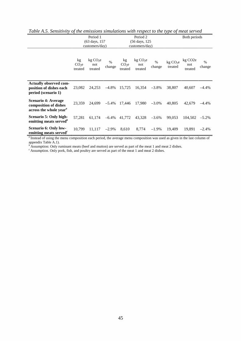
45
Table A.5. Sensitivity of the emissions simulations with respect to the type of meat served
a Instead of using the menu composition each period, the average menu composition was used as given in the last column of appendix Table A.1). b Assumption: Only ruminant meats (beef and mutton) are served as part of the meat 1 and meat 2 dishes. c Assumption. Only pork, fish, and poultry are served as part of the meat 1 and meat 2 dishes.
Period 1 (63 days, 157
customers/day)
Period 2 (56 days, 125
customers/day)
Both periods
kg CO2e
treated
kg CO2e not
treated
% change
kg CO2e
treated
kg CO2e not
treated
% change
kg CO2e treated
kg CO2e not
treated
% change
Actually observed com-position of dishes each period (scenario 1)
23,082 24,253 –4.8% 15,725 16,354 –3.8% 38,807 40,607 –4.4%
Scenario 4: Average composition of dishes across the whole yeara
23,359 24,699 –5.4% 17,446 17,980 –3.0% 40,805 42,679 –4.4%
Scenario 5: Only high-emitting meats servedb
57,281 61,174 –6.4% 41,772 43,328 –3.6% 99,053 104,502 –5.2%
Scenario 6: Only low-emitting meats servedc
10,799 11,117 –2.9% 8,610 8,774 –1.9% 19,409 19,891 –2.4%

46
Figure A.2. Share of meat 2 dishes sold across period by type of meat offered, treated restau-rant
Note: The short dashed lines represent the mean share of meat 2 dishes sold in period 0; long dashed lines, the mean share sold in period 1; and dotted lines, mean shares sold in period 2. Error bars represent 0.95 confidence intervals around the mean for each type.