novel turbomachinery concepts for highly …novel turbomachinery concepts for highly integrated...
TRANSCRIPT

Novel Turbomachinery Concepts for Highly Integrated
Airframe/Propulsion Systems
by
Parthiv Narendra Shah
B.S. Aerospace Engineering, University of Virginia (1994)M.S. Mechanical Engineering, Rutgers University (1998)
Submitted to the Department of Mechanical Engineeringin partial fulfillment of the requirements for the degree of
Doctor of Philosophy
at the
MASSACHUSETTS INSTITUTE OF TECHNOLOGY
February 2007
c© Massachusetts Institute of Technology 2007. All rights reserved.
Author . . . . . . . . . . . . . . . . . . . . . . . . . . . . . . . . . . . . . . . . . . . . . . . . . . . . . . . . . . . . . . . . . . . . . . . . . . . . . . . . . . . . . . . . . .Department of Mechanical Engineering
October 4, 2006
Certified by . . . . . . . . . . . . . . . . . . . . . . . . . . . . . . . . . . . . . . . . . . . . . . . . . . . . . . . . . . . . . . . . . . . . . . . . . . . . . . . . . . . . .Zoltan SpakovszkyAssociate Professor
Thesis Supervisor
Certified by . . . . . . . . . . . . . . . . . . . . . . . . . . . . . . . . . . . . . . . . . . . . . . . . . . . . . . . . . . . . . . . . . . . . . . . . . . . . . . . . . . . . .Choon Sooi Tan
Senior Research EngineerThesis Supervisor
Certified by . . . . . . . . . . . . . . . . . . . . . . . . . . . . . . . . . . . . . . . . . . . . . . . . . . . . . . . . . . . . . . . . . . . . . . . . . . . . . . . . . . . . .John Brisson II
Associate ProfessorDoctoral Committee Chair
Accepted by . . . . . . . . . . . . . . . . . . . . . . . . . . . . . . . . . . . . . . . . . . . . . . . . . . . . . . . . . . . . . . . . . . . . . . . . . . . . . . . . . . . . .Lallit Anand
Chairman, Department Committee on Graduate Students

2

Novel Turbomachinery Concepts for Highly Integrated
Airframe/Propulsion Systems
by
Parthiv Narendra Shah
Submitted to the Department of Mechanical Engineering on October 4, 2006,in partial fulfillment of the requirements for the degree of Doctor of Philosophy
Abstract
Two novel turbomachinery concepts are presented as enablers to advanced flight missions requiringintegrated airframe/propulsion systems. The first concept is motivated by thermal managementchallenges in low-to-high Mach number (4+) aircraft. The idea of compressor cooling combinesthe compressor and heat exchanger function to stretch turbopropulsion system operational limits.Axial compressor performance with blade passage heat extraction is assessed with computationalexperiments and meanline modeling. A cooled multistage compressor with adiabatic design point isfound to achieve higher pressure ratio, choking mass flow, and efficiency (referenced to an adiabatic,reversible process) at fixed corrected speed, with greatest benefit occurring through front-stagecooling. Heat removal equal to one percent of inlet stagnation enthalpy flux in each of the firstfour blade rows suggests pressure ratio, efficiency, and choked flow improvements of 23%, 12%, and5% relative to a baseline, eight-stage compressor with pressure ratio of 5. Cooling is also found tounchoke rear stages at low corrected speed. Heat transfer estimations indicate that surface arealimitations and temperature differences favor rear-stage cooling and suggest the existence of anoptimal cooling distribution.
The second concept is a quiet drag device to enable slow and steep approach profiles for func-tionally quiet civil aircraft. Deployment of such devices in clean airframe configuration reducesaircraft source noise and noise propagation to the ground. The generation of swirling outflow froma duct, such as an aircraft engine, is conceived to have high drag and low noise. The simplestconfiguration is a ram pressure driven duct with non-rotating swirl vanes, a so-called swirl tube.A device aerodynamic design is performed using first principles and CFD. The swirl-drag-noiserelationship is quantified through scale-model aerodynamic and aeroacoustic wind tunnel tests.The maximum measured stable flow drag coefficient is 0.83 at exit swirl angles close to 50. Theacoustic signature, extrapolated to full-scale, is found to be well below the background noise of awell populated area, demonstrating swirl tube conceptual feasibility. Vortex breakdown is found tobe the aerodynamically and acoustically limiting physical phenomenon, generating a white-noisesignature that is ∼ 15 dB louder than a stable swirling flow.
Thesis Supervisor: Zoltan SpakovszkyTitle: Associate Professor
Thesis Supervisor: Choon Sooi TanTitle: Senior Research Engineer
3

4

Acknowledgments
Between July 6 and July 14, 2006, I took a thesis writing retreat at the Sheraton in terminal
3 of Toronto Pearson International Airport. Writing began in earnest there, and this un-
conventional vacation gave me perspective on why my research was relevant to aviation. It
also reminded me that I got into this field because I like airplanes. From my hotel window,
like a kid, I watched the big planes come and go, and on Airport Road I accidentally found
the place where the locals knew you could see (and hear) 747s and A340s land right over
your head. So my first acknowledgement goes to the manager of the Sheraton at YYZ, for
heeding my complaints for a room with a view.
Being a graduate student in the MIT Gas Turbine Laboratory has been a great adventure
from the beginning, and for this I’d like to first thank my two thesis supervisors, Professor
Zoltan Spakovszky and Dr. Choon Tan, for their technical support and their friendship.
Zolti has shown great enthusiasm for my work, and his approach really allowed our meetings
to be forums for new ideas and thinking to emerge. Choon has also been a great advisor
and mentor who has taught me how to communicate my thoughts clearly and effectively.
Professor John Brisson has spent many hours with me in his office discussing my research.
His friendly manner, guidance and positivity have always been encouraging. Professor Ed
Greitzer has asked probing questions that have helped me to understand my own work
better, both in classes and in the Silent Aircraft Initiative engine team meetings. Professor
Frank Marble was kind enough to meet with me and give feedback on the compressor cooling
project. Professor Nick Cumpsty also gave excellent feedback. Professor Jack Kerrebrock
gave us the original inspiration to look into swirling flows, and discussed vane design with
me. Professor Mark Drela helped me with MTFLOW, a key design tool for the swirl tube.
Dr. Yifang Gong has often provided me with ideas to resolve CFD issues.
At NASA Glenn, the compressor cooling work was supported under grant NAG3-2767,
and I gratefully acknowledge the oversight of Dr. Ken Suder and Dr. Arun Sehra. Also,
Dr. John Adamczyk gave input and encouraged me to dig deeper into the definition of
non-adiabatic compressor efficiency, Dr. Louis Larosilier provided good discussion on loss
5

modeling, and Dr. Rod Chima provided me a grid for the Stage 35 compressor.
At NASA Langley, the swirl tube work was supported under contract NAS1-02044, and
I am grateful to our contract monitors Dr. Russell Thomas and Dr. Henry Haskins. In
addition, Dr. Tom Brooks and Tony Humphreys provided great technical guidance at the
world class Quiet Flow Facility (QFF). The crew of the QFF was also a pleasure to work
with, including Dan Stead, Larry Becker, Dennis Kuchta, Jaye Moen, and of course, Ronnie
Geouge, who is in a league by himself in terms of test support and sense of humor.
At Pratt and Whitney and UTRC, I am thankful for the support of Dr. Wes Lord, Dr.
Jinzhang Feng, Dr. Jayant Sabnis, Sanjay Hingorani, Dr. Bob Schlinker, and Prof. Thomas
Barber. Also during my time at Rutgers, Professor Timothy Wei taught me a lot about
being an engineer.
The infinite support of Leslie Regan and Joan Kravit of the Mechanical Engineering
graduate office is appreciated. I would also like to acknowledge the support of the Mechanical
Engineering department head, Professor Rohan Abeyaratne, for helping me to secure the last
six weeks of my funding at MIT. Dean Blanche Staton was also very helpful in this matter.
The GTL staff has been super-supportive over the years. Special thanks go to Lori
Martinez and Holly Anderson for their all around know-how within the lab.
GTL students have been great sources of friendship. Big thanks go to Darius Mobed, my
swirl tube colleague. The model fabrication and experiments would not have been a success
without his talents. Other students and post-docs that I have shared good times with, both
at GTL and beyond, and in no particular order, include Alexi, Sean, Justin, Adrian, Jessica,
Boris, Vai-man, Ryan, Anya, Jim, Angelique, Barbara, Francois, Alphonso, Trevor, Juan,
Caitlyn, Joe, Keen Ian, and Josep.
To my parents, Naren and Neeta Shah, goes my heartfelt love and appreciation for their
support. Their unconditional love and dedication got me to this stage in my life.
Finally, to my partner, soul mate, fiancee, and best friend, Amy... thanks for all your
support during the highs and lows, quals, thesis writing, long hours, and all the joys of
completing this endeavor... I love you.
6

Contents
Acknowledgements 5
List of Figures 10
List of Tables 22
1 Introduction 31
1.1 Background . . . . . . . . . . . . . . . . . . . . . . . . . . . . . . . . . . . . 31
1.2 Thesis Contributions . . . . . . . . . . . . . . . . . . . . . . . . . . . . . . . 32
1.3 Synopsis of Thesis Chapters . . . . . . . . . . . . . . . . . . . . . . . . . . . 33
2 Mission 1: Low-to-High Mach Number Flight 37
2.1 Overview . . . . . . . . . . . . . . . . . . . . . . . . . . . . . . . . . . . . . . 38
2.2 Previous Work . . . . . . . . . . . . . . . . . . . . . . . . . . . . . . . . . . 40
2.3 Mission Profile . . . . . . . . . . . . . . . . . . . . . . . . . . . . . . . . . . 42
2.4 Pre-cooled Turbojet (PCTJ) . . . . . . . . . . . . . . . . . . . . . . . . . . . 46
2.4.1 Modification of Ideal SSTJ Cycle for Compressor Pre-cooling . . . . . 46
2.4.2 Specific Thrust Requirements . . . . . . . . . . . . . . . . . . . . . . 50
2.5 Compressor Cooling: The Idea . . . . . . . . . . . . . . . . . . . . . . . . . . 56
2.5.1 Compressor Cooling vs. Pre-Cooling . . . . . . . . . . . . . . . . . . 56
2.5.2 Diffusing Passage Heat Extraction . . . . . . . . . . . . . . . . . . . . 60
2.5.3 Research Questions . . . . . . . . . . . . . . . . . . . . . . . . . . . . 62
2.5.4 Challenges and Unknowns . . . . . . . . . . . . . . . . . . . . . . . . 62
7

2.6 Chapter Summary . . . . . . . . . . . . . . . . . . . . . . . . . . . . . . . . 63
3 Compressor Cooling: A Novel Turbomachinery Concept for Mission 1 65
3.1 Objectives . . . . . . . . . . . . . . . . . . . . . . . . . . . . . . . . . . . . . 66
3.2 Technical Approach . . . . . . . . . . . . . . . . . . . . . . . . . . . . . . . . 67
3.3 Blade Passage Flows with Heat Extraction . . . . . . . . . . . . . . . . . . . 69
3.3.1 Cascade Cases . . . . . . . . . . . . . . . . . . . . . . . . . . . . . . . 69
3.3.2 Bulk Performance . . . . . . . . . . . . . . . . . . . . . . . . . . . . . 72
3.3.3 Entropy Generation . . . . . . . . . . . . . . . . . . . . . . . . . . . . 77
3.3.4 Generic Rules for Blade Passage Loss and Deviation . . . . . . . . . . 81
3.4 On- and Off- Design Meanline Analysis . . . . . . . . . . . . . . . . . . . . . 85
3.4.1 Single Stage Fan . . . . . . . . . . . . . . . . . . . . . . . . . . . . . 87
3.4.2 Eight Stage Compressor . . . . . . . . . . . . . . . . . . . . . . . . . 90
3.5 Three Dimensional Flow Computations . . . . . . . . . . . . . . . . . . . . . 96
3.6 Heat Transfer Considerations . . . . . . . . . . . . . . . . . . . . . . . . . . 100
3.7 Efficiency Metrics for Non-adiabatic Compressors . . . . . . . . . . . . . . . 103
3.8 Summary of Major Findings . . . . . . . . . . . . . . . . . . . . . . . . . . . 106
4 Mission 2: Quiet Civil Aircraft 107
4.1 Mission Overview and Previous Work . . . . . . . . . . . . . . . . . . . . . . 108
4.2 Quiet Approach Trajectory . . . . . . . . . . . . . . . . . . . . . . . . . . . . 113
4.3 Swirl Tube: The Idea . . . . . . . . . . . . . . . . . . . . . . . . . . . . . . . 119
4.3.1 Research Questions . . . . . . . . . . . . . . . . . . . . . . . . . . . . 123
4.3.2 Challenges and Unknowns . . . . . . . . . . . . . . . . . . . . . . . . 123
4.4 Preliminary Model of Ducted Drag Generator . . . . . . . . . . . . . . . . . 124
4.4.1 Control Volume Analysis of Ducted Drag Generator . . . . . . . . . . 126
4.4.2 Drag Generating Axial Exhaust Flow Devices . . . . . . . . . . . . . 129
4.4.3 Swirling Flow Dynamics . . . . . . . . . . . . . . . . . . . . . . . . . 134
4.4.4 Drag Generating Swirling Exhaust Flow Devices . . . . . . . . . . . . 142
8

4.5 Chapter Summary . . . . . . . . . . . . . . . . . . . . . . . . . . . . . . . . 155
5 Swirl Tube: A Novel Turbomachinery Concept for Mission 2 159
5.1 Objectives . . . . . . . . . . . . . . . . . . . . . . . . . . . . . . . . . . . . . 160
5.2 Technical Approach . . . . . . . . . . . . . . . . . . . . . . . . . . . . . . . . 160
5.3 Swirl Tube Aerodynamics . . . . . . . . . . . . . . . . . . . . . . . . . . . . 163
5.3.1 Two Dimensional Axisymmetric Computations . . . . . . . . . . . . . 164
5.3.2 3D Vane Design Methodology . . . . . . . . . . . . . . . . . . . . . . 172
5.3.3 Three Dimensional CFD Computations . . . . . . . . . . . . . . . . . 175
5.3.4 Model Scale Wind Tunnel Testing . . . . . . . . . . . . . . . . . . . . 183
5.4 Swirl Tube Acoustics . . . . . . . . . . . . . . . . . . . . . . . . . . . . . . . 199
5.4.1 Swirl Mixing Noise Models based on Lighthill’s Acoustic Analogy . . 201
5.4.2 Model Scale Acoustic Testing . . . . . . . . . . . . . . . . . . . . . . 208
5.5 Swirl Tube System Integration . . . . . . . . . . . . . . . . . . . . . . . . . . 228
5.5.1 Upstream Fan Stage Interaction . . . . . . . . . . . . . . . . . . . . . 228
5.5.2 Comparison to Thrust Reverser . . . . . . . . . . . . . . . . . . . . . 234
5.6 Summary of Major Findings . . . . . . . . . . . . . . . . . . . . . . . . . . . 241
6 Summary and Conclusions of the Thesis 243
6.1 Compressor Cooling . . . . . . . . . . . . . . . . . . . . . . . . . . . . . . . 243
6.1.1 Summary of Research . . . . . . . . . . . . . . . . . . . . . . . . . . . 243
6.1.2 Summary of Contributions . . . . . . . . . . . . . . . . . . . . . . . . 245
6.1.3 Recommendations for Future Work . . . . . . . . . . . . . . . . . . . 245
6.2 Swirl Tube . . . . . . . . . . . . . . . . . . . . . . . . . . . . . . . . . . . . . 247
6.2.1 Summary of Research . . . . . . . . . . . . . . . . . . . . . . . . . . . 247
6.2.2 Summary of Contributions . . . . . . . . . . . . . . . . . . . . . . . . 248
6.2.3 Recommendations for Future Work . . . . . . . . . . . . . . . . . . . 249
9

10

List of Figures
2-1 Standard atmosphere model showing temperature, pressure, density, vs. al-
titude, and contours of Mach number in the altitude-velocity plane. Symbol
indicates design point of M = 4, h = 25 km. . . . . . . . . . . . . . . . . . . 43
2-2 Selected flight path. Heavy, broken line represents low Mach number trajec-
tory. Heavy, solid line is ρV 2/2 = 28.4 kPa, representing high Mach number
trajectory. Faint broken lines are lines of constant ρV 2/2 in kPa. Faint dash-
dot lines are lines of constant specific energy, in km. . . . . . . . . . . . . . . 44
2-3 Stagnation properties along flight path. . . . . . . . . . . . . . . . . . . . . . 45
2-4 PCTJ schematic. Indicated stations are: 1) Inlet/pre-cooler inlet, 2) pre-
cooler exit/compressor inlet, 3) compressor exit/burner inlet, 4) burner exit/turbine
inlet, 5) turbine exit/nozzle inlet, 7) nozzle exit. . . . . . . . . . . . . . . . . 46
2-5 Specific thrust for ideal SSTJ (solid line) and ideal SSTJ with pre-cooling
(broken line) for given mission. . . . . . . . . . . . . . . . . . . . . . . . . . 49
2-6 Mach number dependence of drag model used in mission analysis, based on a
typical supersonic jet aircraft [59, p. 86]. . . . . . . . . . . . . . . . . . . . . 51
2-7 Uncooled available (solid line), uncooled required (broken line), and pre-cooled
(dash-dot line) specific thrust vs. Mach number for chosen vehicle in steady,
level flight on selected trajectory. . . . . . . . . . . . . . . . . . . . . . . . . 53
2-8 Pre-cooling temperature ratio for chosen vehicle in steady, level flight on se-
lected trajectory. . . . . . . . . . . . . . . . . . . . . . . . . . . . . . . . . . 54
2-9 Pre-cooler requirements along selected trajectory. . . . . . . . . . . . . . . . 55
11

2-10 CCTJ and HCTJ schematics. Indicated stations are: 1) Inlet/pre-cooler inlet,
2) pre-cooler exit/compressor inlet, 3) compressor exit/burner inlet, 4) burner
exit/turbine inlet, 5) turbine exit/nozzle inlet, 7) nozzle exit. . . . . . . . . . 55
2-11 Temperature-entropy diagram for for standard compression (A-B), compres-
sion with pre-cooling (A-C-D), and interspersed cooling and compression in
N steps (A-E-...-F). . . . . . . . . . . . . . . . . . . . . . . . . . . . . . . . . 56
2-12 Same as Fig 2-11 with real precooled compression process (A-C′-D′) and com-
pression followed by constant pressure post-cooling (A-B-B′). . . . . . . . . . 58
2-13 Critical pre-cooling stagnation pressure recovery vs. cooling load. Operation
above the line favors real pre-cooled compression, while operation below the
line favors a lossless post-cooled compressor (a limiting case of cooled com-
pressor with no new loss generating gas path surfaces). Plot is made on an
equal work, equal cooling basis for pressure ratios of 2, 5, and 8. . . . . . . . 59
2-14 Control volume of a diffusing blade passage with heat extraction. Upstream
and downstream flow angles, αu and αd, respectively, are assumed fixed. . . . 60
2-15 Cooled stator passage control volume model. . . . . . . . . . . . . . . . . . . 61
3-1 Compressor cooling technical road map. . . . . . . . . . . . . . . . . . . . . 67
3-2 Computational grids for cascades 1 and 2. . . . . . . . . . . . . . . . . . . . 70
3-3 Total pressure reduction coefficient, ω, vs. flow inlet angle, βin, at low (0.4)
and high (0.8) inlet Mach number, for cascades 1 and 2. . . . . . . . . . . . . 73
3-4 Non-dimensional cooling, q∗, vs. flow inlet angle, βin, at low (0.4) and high
(0.8) inlet Mach number, for cascade 2 with Twall/Tt,in = 0.5 cooling boundary
condition. . . . . . . . . . . . . . . . . . . . . . . . . . . . . . . . . . . . . . 74
3-5 CFD estimated (solid, Equation 3.4) vs. analytical one dimensional channel
flow sensitivity coefficient (dashed, Equation 3.5). Data normalized to q∗ =
q/ht,in = −0.001. . . . . . . . . . . . . . . . . . . . . . . . . . . . . . . . . . 75
12

3-6 Adiabatic vs. cooled exit Mach number, Mout, for cascade 2. Solid line with
circles represents adiabatic boundary conditions; dashed line with triangles
represents blade surface cooling. Wall temperature BC is Twall/Tt,in = 0.5. . 77
3-7 Cascade 2, computed entropy generation vs. incidence at low (0.4) and high
(0.8) inlet Mach number using net entropy flux method (solid lines given
by Equation 3.7) and direct volume integration(dashed lines given by Equa-
tion 3.8). Adiabatic (red) and cooled (blue, Twall/Tt,in = 0.5) cases shown. . 79
3-8 Cascade 2, viscous (black), and thermal (gray) dissipation vs. incidence at
low (0.4) and high (0.8) inlet Mach number. Plots on left are adiabatic wall
BC; plots on right are Twall/Tt,in = 0.5. . . . . . . . . . . . . . . . . . . . . . 80
3-9 Generic adiabatic vs. cooled loss buckets derived from cascade 1 performance.
Solid line with circles represents adiabatic boundary conditions; dashed line
with triangles represents blade surface cooling. Non-dimensional cooling rate
is q∗ = qht,in
= −0.001. . . . . . . . . . . . . . . . . . . . . . . . . . . . . . . 83
3-10 Adiabatic change in deviation, ∆δa, (relative to Carter’s rule) for cascade 1. 84
3-11 Additional flow turning from cooling, ∆βcool = −∆δcool, for cascade 1, q∗ =
−0.001. Dotted lines with symbols are CFD results. Heavy solid lines are
average values (used in meanline analysis) for given inlet Mach numbers. . . 85
3-12 Eight stage compressor meridional layout. First stage also analyzed as a single
stage fan. . . . . . . . . . . . . . . . . . . . . . . . . . . . . . . . . . . . . . 86
3-13 Single stage compressor map, with and without cooling. Solid line is adiabatic;
Dashed line is q∗ = −0.0025. 100%, 80%, and 60% Nc lines are shown. . . . . 88
3-14 Single stage compressor map, with and without different effects from cooled
cascade performance. Solid red line is adiabatic; Solid green line shows effect
of change in deviation due to cooling; Dashed black line shows effect of change
in ω due to cooling; Dashed blue line shows both effects. 100%, 80%, and 60%
Nc lines are shown. In cooled cases, q∗ = −0.0025. . . . . . . . . . . . . . . . 90
3-15 Cooling schemes studied in eight stage compressor meanline model. . . . . . 91
13

3-16 Eight stage efficiency map, with and without cooling. Dash-dot line is adia-
batic; solid line is q∗ = −0.01 in last two stages; dashed line is q∗ = −0.0025
in all stages; solid line with circles is q∗ = −0.01 in first two stages. 100%,
80%, and 60% Nc lines are shown. . . . . . . . . . . . . . . . . . . . . . . . . 92
3-17 Eight stage compressor map, with and without cooling. Solid red line is
adiabatic; Dashed-dot green line is q∗ = −0.01 in last two stages; Dashed blue
line is q∗ = −0.0025 in all stages; Solid black line is q∗ = −0.01 in first two
stages. 100%, 80%, and 60% Nc lines are shown. . . . . . . . . . . . . . . . . 93
3-18 Rotor 35 geometry and boundary conditions (single passage periodic) for non-
adiabatic case. Filled static temperature contours on wall boundaries (hub,
casing, and blade surfaces) show BC of 100 K on blade and middle portion of
outer casing surface. Positive x-axis is downstream axial direction. . . . . . . 97
3-19 Rotor 35 pressure ratio map. . . . . . . . . . . . . . . . . . . . . . . . . . . . 98
3-20 Rotor 35 efficiency map. . . . . . . . . . . . . . . . . . . . . . . . . . . . . . 100
3-21 Blade surface non-dimensional heat transfer per unit solidity vs. wall tem-
perature at various turbulent Reynolds numbers, generated using Reynolds
analogy over a flat plate. . . . . . . . . . . . . . . . . . . . . . . . . . . . . . 102
4-1 Comparison between Cambridge-MIT Silent Aircraft conceptual design with
embedded engines, a blended wing body (BWB) aircraft with podded engines,
and a conventional tube and wing aircraft. . . . . . . . . . . . . . . . . . . . 109
4-2 Polar directivity plot of Lockheed L-1011 overall sound pressure level (OASPL)
for two different flap angle settings, suggesting a strong correlation between
noise and drag. Figure adopted from Smith [81]. . . . . . . . . . . . . . . . . 111
4-3 Aircraft force balance on approach. . . . . . . . . . . . . . . . . . . . . . . . 115
14

4-4 Iso-contours of quiet drag coefficient, CD,quiet (black) and estimated noise re-
duction (red) as a function of velocity ratio and approach angle for CD,0 =
0.01, θref = 3, and Vref = 1.23 · Vstall = 60.8 m/s, per Equation 4.10. SAX
landing weight is 125,000 kg, wing area is 836 m2, and k for the drag polar
is 0.064. Blue arrows indicate three different means to achieve 5 dB noise
reduction. . . . . . . . . . . . . . . . . . . . . . . . . . . . . . . . . . . . . . 117
4-5 Drag-generating swirling flow concepts. . . . . . . . . . . . . . . . . . . . . . 121
4-6 Propulsion system integrated swirl tube concept with deployable swirl vanes,
having functionality to actuate to a closed position to serve as a thrust reverser
blocker door. . . . . . . . . . . . . . . . . . . . . . . . . . . . . . . . . . . . 122
4-7 Control volume of cross sectional area, A, around ducted quiet drag device
containing an actuator disk. Pylon holds device in static equilibrium relative
to freestream flow. Stations u and d are far upstream of device and at the
duct exit, respectively. Stations 1 and 2 are just upstream and downstream
of actuator disk, respectively. Af and Ad are actuator disk face area and duct
exit area, respectively. . . . . . . . . . . . . . . . . . . . . . . . . . . . . . . 127
4-8 Drag coefficient as a function of throttling parameters Vz,d/V∞ and ω for
purely axial exhaust flow for different area ratios. Peak drag coefficient equals
0.5 times area ratio, implying an exit area increase leads to higher maximum
drag. . . . . . . . . . . . . . . . . . . . . . . . . . . . . . . . . . . . . . . . . 131
4-9 Drag coefficient breakdown for purely axial exhaust flow devices indicates
that total drag is comprised of a drag force on the actuator disk and a thrust
force on the nacelle. Shaded area indicates likely region of vortex shedding
instability, as suggested by Figure 4-10. . . . . . . . . . . . . . . . . . . . . . 132
4-10 Instantaneous unsteady contours of dimensionless entropy, Tt,∞s/V2∞, on 2D
CFD of deficit flow with varying velocity ratio at device scale Reynolds num-
ber. Nozzle height is 2.16 meters. Computations indicate that vortex shedding
instability develops at velocity ratios . 0.25. . . . . . . . . . . . . . . . . . . 133
15

4-11 Types of vortex breakdown, adopted from Leibovich [48]. . . . . . . . . . . . 137
4-12 Types of vortex breakdown from low to high swirl, adopted from Hall [28]
based on the photographs of Sarpkaya [74]. . . . . . . . . . . . . . . . . . . . 138
4-13 Profiles of axial velocity, circumferential velocity, pressure coefficient, and
swirl parameter for analytical swirl tube model with Burger vortex exit flow
parameters of ω = −∆pt/q∞ = 0.08, r∗crit = 0.50, and K∗c = 0.77, yielding
drag coefficient of CD = 0.8. . . . . . . . . . . . . . . . . . . . . . . . . . . . 146
4-14 Contours of predicted total drag coefficient (CD, dashed red) and swirl para-
meter at r = rcrit (S, solid black) in (K∗c , r
∗crit) space for ram pressure driven
swirl tube having ω = 0.08. Triangle indicates point with CD = 0.8 and
rcrit = 0.5, whose radial profiles are presented in Figure 4-13. Heavy, dashed
blue line indicates (K∗c )max threshold. . . . . . . . . . . . . . . . . . . . . . . 148
4-15 Contours of predicted total drag coefficient (CD, dashed red) and capture
streamtube to actuator disk area ratio (Acapt/Af , solid black) in (K∗c , r
∗crit)
space for ram pressure driven swirl tube having ω = 0.08. Triangle indicates
point with CD = 0.8 and rcrit = 0.5. Heavy, dashed blue line indicates (K∗c )max
threshold. . . . . . . . . . . . . . . . . . . . . . . . . . . . . . . . . . . . . . 149
4-16 Contours of predicted drag coefficients from pressure defect (CD,press., solid
black) and net axial momentum flux (CD,ax. mom., dashed red) in (K∗c , r
∗crit)
space for ram pressure driven swirl tube having ω = 0.08. Triangle indicates
point with CD = 0.8 and rcrit = 0.5. Heavy, dashed blue line indicates (K∗c )max
threshold. . . . . . . . . . . . . . . . . . . . . . . . . . . . . . . . . . . . . . 150
4-17 Contours of predicted total drag coefficient (CD) in (S, ω) space for ram pres-
sure driven swirl tube having r/rcrit = 0.5. . . . . . . . . . . . . . . . . . . . 151
4-18 Contours of predicted total drag coefficient, CD (dashed red), and swirl para-
meter, S (solid black), in (K∗c ,∆pt/q∞) space for pumped or throttled swirl
tube with r/rcrit = 0.5. Dashed blue line indicates (K∗c )max threshold. . . . . 152
16
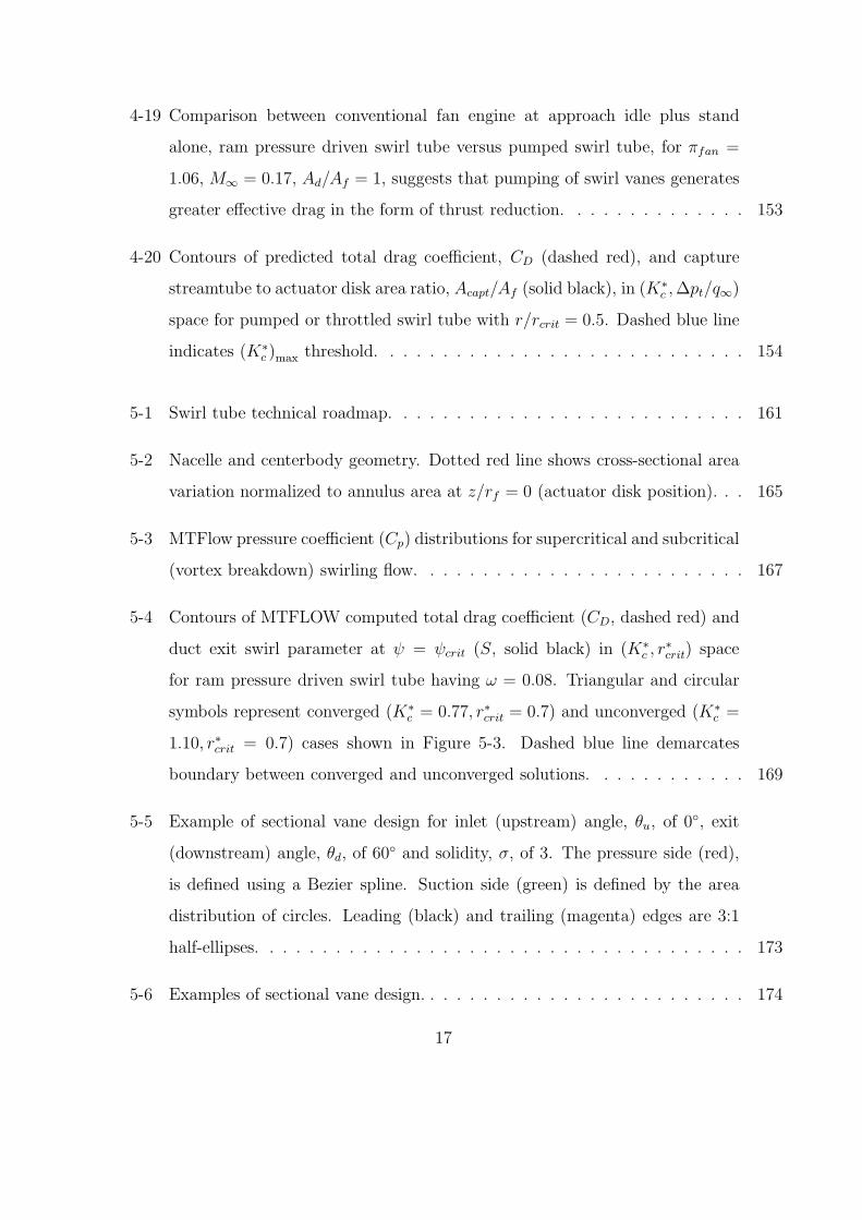
4-19 Comparison between conventional fan engine at approach idle plus stand
alone, ram pressure driven swirl tube versus pumped swirl tube, for πfan =
1.06, M∞ = 0.17, Ad/Af = 1, suggests that pumping of swirl vanes generates
greater effective drag in the form of thrust reduction. . . . . . . . . . . . . . 153
4-20 Contours of predicted total drag coefficient, CD (dashed red), and capture
streamtube to actuator disk area ratio, Acapt/Af (solid black), in (K∗c ,∆pt/q∞)
space for pumped or throttled swirl tube with r/rcrit = 0.5. Dashed blue line
indicates (K∗c )max threshold. . . . . . . . . . . . . . . . . . . . . . . . . . . . 154
5-1 Swirl tube technical roadmap. . . . . . . . . . . . . . . . . . . . . . . . . . . 161
5-2 Nacelle and centerbody geometry. Dotted red line shows cross-sectional area
variation normalized to annulus area at z/rf = 0 (actuator disk position). . . 165
5-3 MTFlow pressure coefficient (Cp) distributions for supercritical and subcritical
(vortex breakdown) swirling flow. . . . . . . . . . . . . . . . . . . . . . . . . 167
5-4 Contours of MTFLOW computed total drag coefficient (CD, dashed red) and
duct exit swirl parameter at ψ = ψcrit (S, solid black) in (K∗c , r
∗crit) space
for ram pressure driven swirl tube having ω = 0.08. Triangular and circular
symbols represent converged (K∗c = 0.77, r∗crit = 0.7) and unconverged (K∗
c =
1.10, r∗crit = 0.7) cases shown in Figure 5-3. Dashed blue line demarcates
boundary between converged and unconverged solutions. . . . . . . . . . . . 169
5-5 Example of sectional vane design for inlet (upstream) angle, θu, of 0, exit
(downstream) angle, θd, of 60 and solidity, σ, of 3. The pressure side (red),
is defined using a Bezier spline. Suction side (green) is defined by the area
distribution of circles. Leading (black) and trailing (magenta) edges are 3:1
half-ellipses. . . . . . . . . . . . . . . . . . . . . . . . . . . . . . . . . . . . . 173
5-6 Examples of sectional vane design. . . . . . . . . . . . . . . . . . . . . . . . . 174
17

5-7 Loss factor and Zweifel coefficient as a function of axial chord to spacing for
two types of turbine vanes. Design range is shaded. The plot suggests that
a turbine vane with inlet and exit angles of 0 and 60, respectively, and
axial chord-to-spacing ratios of 2.6 to 4 has sufficient Zweifel coefficient and
reasonably low losses. Figure adopted from Kerrebrock [47] . . . . . . . . . . 174
5-8 Typical CFD domain replicated to show ten periodic passages. . . . . . . . . 176
5-9 Mach number on periodic boundary of CFD cases. . . . . . . . . . . . . . . . 178
5-10 Swirl parameter on periodic boundary of CFD cases. . . . . . . . . . . . . . 179
5-11 Pressure coefficient on periodic boundary of CFD cases. . . . . . . . . . . . . 179
5-12 Pressure coefficient, Cp, on surfaces of swirl tube with 47 vane angle show
low pressure at vane hub and aft centerbody. Radial extent of pressure defect
is seen in plane 0.5 duct diameters downstream of exit. Maximum pressure
defect in downstream plane is Cp ≈ −3.5. . . . . . . . . . . . . . . . . . . . . 180
5-13 MTFlow vs CFD comparisons for case with 47 swirl vanes. . . . . . . . . . 181
5-14 WBWT wind tunnel experimental set-up. . . . . . . . . . . . . . . . . . . . 184
5-15 Flow visualization close to the centerline axis identifies a coherent vortex core
within a steady swirling flow for the stable flow cases (34, 41, and 47 swirl
vanes) and a large unsteady core for the cases with vortex breakdown (57
and 64 swirl vanes). . . . . . . . . . . . . . . . . . . . . . . . . . . . . . . . 185
5-16 Flow visualization at the outer radius identifies a tightly spiraling, steady
swirling flow for stable cases (34, 41, and 47 swirl vanes) and indirectly
infers an outer coherent swirling flow for vortex breakdown cases (57 and 64
swirl vanes). . . . . . . . . . . . . . . . . . . . . . . . . . . . . . . . . . . . . 186
5-17 Hot-wire traverse locations for steady and unsteady measurements. All mea-
surements are taken in the vertical plane that passes through the swirl tube
centerline. . . . . . . . . . . . . . . . . . . . . . . . . . . . . . . . . . . . . . 188
18

5-18 Axial velocity, circumferential velocity, and computed swirl parameter (S) vs.
radial location for case with 34 swirl vanes. Top row, z/D = 0.5, bottom
row z/D = 1.0. . . . . . . . . . . . . . . . . . . . . . . . . . . . . . . . . . . 189
5-19 Axial velocity, circumferential velocity, and computed swirl parameter (S) vs.
radial location for case with 47 swirl vanes. Top row, z/D = 0.5, bottom
row z/D = 1.0. . . . . . . . . . . . . . . . . . . . . . . . . . . . . . . . . . . 190
5-20 Axial velocity, circumferential velocity, and computed swirl parameter (S) vs.
radial location for case with 57 swirl vanes. Top row, z/D = 0.5, bottom
row z/D = 1.0. . . . . . . . . . . . . . . . . . . . . . . . . . . . . . . . . . . 191
5-21 Power spectra of unsteady axial and tangential velocity in core region, r∗ = 0,
at axial location one diameter downstream of nozzle exit, z/D = 1.0. Data is
presented at constant bandwidth of 2.44 Hz. . . . . . . . . . . . . . . . . . . 192
5-22 Power spectra of unsteady axial and tangential velocity in shear layer region,
r∗ = 1, at axial location one diameter downstream of nozzle exit, z/D = 1.0. 193
5-23 Model-scale drag coefficient vs. swirl vane angle shows measured drag coeffi-
cient of 0.83 for highest stable flow swirl vane angle (47). CFD drag coefficient
adjusted for model-scale is shown for converged, stable flow cases (34, 47,
and 53 swirl vane angles). . . . . . . . . . . . . . . . . . . . . . . . . . . . . 198
5-24 Comparison between computed jet noise spectra using Tam’s fine scale tur-
bulence noise source, Morris-Farassat source term, and Stone and SAE round
single jet empirical models. Jet diameter is 1 meter. Spectra scaled to r = 1
m, for an observer angle of θ = 90. . . . . . . . . . . . . . . . . . . . . . . . 205
5-25 Hybrid Tam + Tanna model prediction of stable swirling flow noise using
2D CFD computation of swirl tube aft geometry. QFF facility background
included for reference. One-third octave band spectra corrected to 1 meter
observer distance at 90 observer location. . . . . . . . . . . . . . . . . . . . 208
19

5-26 Spectral density integrand (at predicted peak noise frequency) for two-dimensional
CFD of swirl tube exit flowfield for case of 47 swirl vanes. Freestream Mach
number is set to 0.17. Axis units are in meters, based on full-scale CFD
geometry of 2.16 m swirl vane outer diameter. . . . . . . . . . . . . . . . . . 209
5-27 Photographs of NASA LaRC QFF setup. . . . . . . . . . . . . . . . . . . . . 210
5-28 QFF directional array polar arc variation capabilities, adopted from [9]. Medium
Aperture Directional Array (MADA) is depicted relative to the free jet with
swirl tube model installed. Vertical free jet flow is from bottom to top. In
this thesis, all data are presented with array in θ = −90 position. . . . . . . 211
5-29 Full-scale (1.2 m diameter) drag coefficient (CD) and overall sound pressure
level (OASPL) vs. swirl angle suggests that a high-drag, low-noise configura-
tion exists at swirl vane angle of 47. Freestream Mach number for OASPL is
0.17. Observer location is 120 m from the source, at sideline angle of θ = −90
(see Figure 5-28). . . . . . . . . . . . . . . . . . . . . . . . . . . . . . . . . . 213
5-30 Model-scale spectra at 47 and 57, Mach=0.17, θ = −90. . . . . . . . . . . 215
5-31 Overall spectral comparison of all swirl tube configurations, constant 17.44
Hz bandwidth, Mach=0.17, θ = −90. . . . . . . . . . . . . . . . . . . . . . . 216
5-32 Full-scale third-octave band autospectra at 47 and 57, Mach=0.17, θ = −90.219
5-33 Mach number scaling of 47 spectra assuming different scaling exponents, n,
per Equation 5.18. All spectra are presented non-dimensionally in a dB/St
basis basis. . . . . . . . . . . . . . . . . . . . . . . . . . . . . . . . . . . . . . 220
5-34 Mach number scaling of 57 spectra assuming n = 7.5 power law, per Equa-
tion 5.18. All spectra are presented non-dimensionally in a dB/St basis. Good
collapse is suggested for 15 < St < 100. . . . . . . . . . . . . . . . . . . . . . 221
5-35 DAMAS integration zones. Zones 1, 2, and 3 correspond to aft, fore, and
pylon regions, respectively. . . . . . . . . . . . . . . . . . . . . . . . . . . . . 223
5-36 DAMAS zone-integrated spectra and source maps, 47 swirl vane angle case,
M = 0.17, θ = −90. . . . . . . . . . . . . . . . . . . . . . . . . . . . . . . . 224
20

5-37 DAMAS zone-integrated spectra and source maps, 57 swirl vane angle case,
M = 0.17, θ = −90. . . . . . . . . . . . . . . . . . . . . . . . . . . . . . . . 225
5-38 Iso-contours of the thrust coefficient (CT ) and captured streamtube area ratio,
for various approach idle pressure ratios and assumed fan stage efficiencies.
Approach Mach number is 0.17. . . . . . . . . . . . . . . . . . . . . . . . . . 229
5-39 Thrust reduction comparison between engine and stand alone, ram pressure-
driven swirl tube (configuration 1) versus propulsion system-integrated swirl
vanes (pumped swirl tube, configuration 2). . . . . . . . . . . . . . . . . . . 230
5-40 Swirl parameter on periodic boundary of ram pressure driven and pumped
swirl tube CFD cases, π = 1.08. . . . . . . . . . . . . . . . . . . . . . . . . . 231
5-41 Mach number on periodic boundary of ram pressure driven and pumped swirl
tube CFD cases, π = 1.08. . . . . . . . . . . . . . . . . . . . . . . . . . . . . 231
5-42 Graphical depiction showing that the effective drag coefficient from a pumped
swirl tube is approximately the difference between the total drag coefficient
and the actuator disk drag coefficient on the fan stage. Negative numbers
indicate net forces in the thrust direction. Freestream Mach number is 0.17. 233
5-43 SAX landing roll velocity vs. distance. . . . . . . . . . . . . . . . . . . . . . 240
21

22
List of Tables
3.1 Average effect of q∗ = −0.001 on flow turning for cascade 1, across a range of
incidences. . . . . . . . . . . . . . . . . . . . . . . . . . . . . . . . . . . . . . 72
3.2 Key single stage fan map parameters at points a through h, as shown in
Figure 3-13. The variables M , i, ∆δ, and ω are Mach number, incidence,
deviation change, and total pressure reduction coefficient, respectively. The
subscripts in and out correspond to the inlet and outlet, respectively. The
subscripts R and S correspond to the rotor and stator, respectively . . . . . 89
3.3 Key eight stage compressor map parameters at adiabatic points i through n, as
shown in Figure 3-17. From top to bottom, sub-tables show rotor incidence,
stator incidence, rotor inlet Mach number, and stator inlet Mach number,
respectively. . . . . . . . . . . . . . . . . . . . . . . . . . . . . . . . . . . . . 94
3.4 Eight stage compressor cooling scheme summary for design corrected speed
line (100% Nc) and design corrected mass flow. . . . . . . . . . . . . . . . . 95
4.1 Silent drag similarity across several aircraft types. The two right most columns
show drag coefficient required to change conventional 3 glideslope to 6, in
terms of wing area and propulsion system fan area. Fan area includes fan
spinner. All numbers are approximate. . . . . . . . . . . . . . . . . . . . . . 120
5.1 Maximum vane turning angle (rounded to nearest degree) associated with
drag coefficient computed by MTFLOW. . . . . . . . . . . . . . . . . . . . . 172
23

5.2 MTFLOW vs. CFD drag coefficient comparison. Total drag coefficient is
given by CD. Pressure and viscous drag coefficients are given as CD,press. and
CD,visc., respectively. . . . . . . . . . . . . . . . . . . . . . . . . . . . . . . . 182
5.3 WBWT test matrix. . . . . . . . . . . . . . . . . . . . . . . . . . . . . . . . 184
5.4 Table of measured and CFD computed drag coefficients for model-scale geom-
etry. All CD values are referenced to the axially projected swirl vane annulus
area. CFD values of viscous drag coefficient, CD,visc., are corrected to model-
scale using Reynolds number correction of Equation 5.4. Pylon drag is shown
for reference only, and is subtracted out of all other cases. . . . . . . . . . . 196
5.5 Pumped swirl tube drag coefficient comparison and breakdown. . . . . . . . 233
5.6 Braking coefficient summary reproduced from Raymer [70], assuming the con-
servative scenario of worn brakes. . . . . . . . . . . . . . . . . . . . . . . . . 236
5.7 Landing roll lengths in meters for various scenarios. Published values from
Jane’s [44] included for comparison. . . . . . . . . . . . . . . . . . . . . . . . 239
24

Nomenclature
Roman
a Speed of sound
A Area
c Chord length; convective speed; speed of sound
cℓ Length scale constant in Tam et al. fine-scale turbulence jet-noise model
cp Specific heat at constant pressure
cτ Time scale constant in Tam et al. fine-scale turbulence jet-noise model
CD Drag coefficient
Cf Skin friction coefficient
CL Lift coefficient
Cp Pressure coefficient
CT Thrust coefficient
CW Weight coefficient
D Drag; diameter
f Frequency
F Thrust; force; function
g Gravitational acceleration constant
h Specific enthalpy; altitude
i Incidence angle; Einstein summation convention index
k Induced drag constant; Turbulence kinetic energy; coefficient
25

K Induced drag constant; Circulation (rVθ)
ℓ Length scale
L Lift
m Mass
m Mass flow
M Mach Number
n Power law exponent
~n Unit normal vector
N Number of blades/vanes
Nc Corrected rotor speed
p Pressure
pt Stagnation pressure
q Dynamic pressure; heat transfer per unit mass
q∗ Non-dimensional heat transfer rate
qw Average wall heat flux (heat transfer rate per unit surface area)
Q Heat transfer rate
r radius, radial coordinate; distance from sound source
R Ideal gas constant (per unit mass)
Re Reynolds number
s Specific entropy
S Swirl parameter; area; wetted area; spectral density
St Stanton number
T Temperature; thrust
T0 Ambient temperature
Tij Lighthill stress tensor
Tt Stagnation temperature
Tx Axial torque
u Velocity
26

V Velocity
wsh Shaft work
W Weight
~x Observer location
z Axial coordinate
Greek
α Swirl angle; angle of attack; Tanna noise modeling parameter
β Flow angle
γ Ratio of specific heats
Γ Circulation
δ Deviation angle
δij Kronecker delta
∆ Difference or change in
ǫ Small perturbation; Dissipation rate (k − ǫ turbulence model)
η Efficiency, induced drag exponent
θ Temperature ratio; circumferential coordinate; polar angle; glideslope angle
µ Density
ν Radian frequency
π Pressure ratio
ρ Density
σ Solidity
τ Temperature ratio; viscous stress; time scale
φ Equivalence ratio
χ Metal angle
ψ Streamfunction; observer angle
27

Ψ Streamfunction for quasi-cylindrical flow
Ω Total pressure reduction coefficient; rotational frequency
ω Rotational shaft speed
Subscripts
0 Ambient condition
a Adiabatic; adjoint Greens function
a.d. Actuator disk
b Blade row
c Compressor face; based on chord length
capt Captured streamtube
comp Compressor face
cool Cooling
crit Critical value
d Downstream; discharge (duct exit)
D Drag
f Fan or actuator disk face
gen (Entropy) generation
H Hub
in Inlet, inflow
lam Laminar
max Maximum
na Non-adiabatic
out Outlet, outflow
press. Pressure component
quiet Used with CD for quiet drag
28

r Radial direction
ref Reference condition
rev Reversible
R Rotor
S Stator
T Tip
turb Turbulent
u Upstream
visc. Viscous component
w Wing
wall Wall value
z Axial direction
θ Circumferential direction
Superscripts
∗ Non-dimensional quantity
Acronyms
BC Boundary Condition
BWB Blended Wing Body Aircraft
CCTJ Compressor-cooled Turbojet
CFD Computational Fluid Dynamics
CMI Cambridge-MIT Institute
HCTJ Hybrid-cooled Turbojet
LHS Left Hand Side
29

MADA Medium Aperture Directional Array
OASPL Overall Sound Pressure Level
PCTJ Pre-cooled Turbojet
QFF NASA Langley Quiet Flow Facility
RANS Reynolds Averaged Navier-Stokes Equations
RHS Right Hand Side
SAE/ARP Society of Automotive Engineers/Aerospace Recommended Practice
SAI Silent Aircraft Initiative
SAX Silent Aircraft eXperimental Design
SPL Sound Pressure Level
SSTJ Single Spool Turbojet
WBWT Wright Brothers Wind Tunnel
Symbols
∇ Del operator
∞ Freestream value
30

Chapter 1
Introduction
1.1 Background
Aircraft design is driven by mission requirements. The mission profile, i.e. the position-
time history through the flight envelope, may depend on myriad requirements such as (i)
payload capacity, (ii) fuel economy, (iii) time to achieve a certain objective, (iv) structural
loading, (v) maximum flight speed, and (vi) maneuverability. In addition to these, noise and
emissions are now at the forefront of technology efforts to minimize adverse environmental
impacts. All aircraft missions, military or commercial, involve a compromise of these and
other requirements.
Conventional aircraft design largely separates the airframe design from the powerplant.
This occurs in part because conventional tube and wing designs have relatively little interfer-
ence between airframe and engine air flows. Today, however, there is increased demand for
unconventional missions, for which vehicle design must be heavily integrated at the system
level.
This thesis presents novel turbomachinery design concepts for two such missions: 1) a
low-to-high Mach number (4+) flight vehicle and 2) a functionally silent1 aircraft. The first
mission addresses the need for the next generation of space-access and high speed interceptor
1Here, the term functionally silent means quieter than the background noise of a well populated urbanarea.
31

vehicles, while the second mission addresses the need for sustained or increased commercial
passenger capacity in the face of increasing population densities near airports and associated
community noise complaints.
For the low-to-high flight Mach number mission, the concept of blade passage surface heat
extraction, so-called compressor cooling, is conceived and assessed as a means to improve
fan/compressor performance, operability, and durability. The idea of compressor cooling is
conceived as a means to sustain the production of specific thrust at high Mach number,
because it can both improve the compressor’s performance as well as reduce compressor
exit temperatures, allowing heat addition without violating engine hot section temperature
limits.
For the functionally silent aircraft mission, a quiet drag device utilizing ducted swirl
vanes, a so-called swirl tube, is conceived, designed, and validated as a means to achieve
the drag necessary for a next-generation aircraft to fly a slower and steeper approach profile
in clean airframe configuration. Flying such a trajectory potentially reduces noise source
strength and increases the attenuation during propagation to the ground. This device is a
key enabler to reducing the need to generate drag on approach through conventional devices
such as flaps, slats, and landing gear, which generally have a strong correlation between drag
and noise.
1.2 Thesis Contributions
The primary contributions of the thesis are:
Compressor Cooling
1. Assessment of the effects of heat extraction on blade passage performance metrics.
2. Development of a first-of-its-kind compressor meanline modeling framework with heat
extraction to assess the on- and off-design behavior of a cooled axial compressor.
32

3. Explanation of the causality between performance implications of heat extraction in
blade passage flows and the behavior of an axial compressor, including a CFD simula-
tion of a three-dimensional rotor passage of practical interest.
4. Establishment of new efficiency metrics for compressors with heat extraction, substan-
tiated by a bookkeeping of entropy generation from viscous and thermal dissipation.
Swirl Tube
1. Successful demonstration of quiet drag coefficient of 0.8 with overall A-weighted sound
pressure level (OASPL) of 42 dBA from a full-scale swirl tube.
2. Quantification of the relationship between swirl angle, drag, and noise for a family of
swirl tube designs.
3. Identification and quantification of acoustic sources associated with the swirling outflow
of a ram pressure driven swirl tube.
4. Identification of the limitations imposed by the vortex breakdown phenomenon on swirl
tube aerodynamic and acoustic performance.
5. Preliminary description of the propulsion-system integrated effect of a fan driven swirl
drag device for slow, steep approaches to reduce aircraft approach noise.
6. Recommendation to integrate swirl vanes into a thrust reverser system to achieve the
dual functionality of drag on approach and thrust reverser blocker doors during landing.
1.3 Synopsis of Thesis Chapters
The thesis is comprised of two major bodies of work, each presented in two chapters. Chap-
ters 2 and 3 present the ideas and outcomes of the compressor cooling project. Chapters 4
and 5 present the ideas and outcomes of the swirl tube project. A description of the remain-
ing chapters is provided below for the reader’s guidance.
33

Compressor Cooling
Chapter 2. This chapter presents background and preliminary analysis of low-to-high
flight Mach number propulsion system configurations to motivate the concept of compressor
cooling. A selected literature review of combined cycle powerplant concepts indicates that
heat extraction, in the form of compression pre-cooling, has been recommended by numerous
authors to extend the vehicle operational Mach number envelope. Compressor cooling, i.e.,
heat extraction within compressor blade passages is thus proposed as a means to achieve the
benefits associated with pre-cooling, without introducing new loss-generating surfaces within
the engine gas path. Analysis indicates that scenarios may exist that favor compressor
cooling or hybrid compressor/pre-cooling, over simple pre-cooling, suggesting benefits in
aero-thermodynamic performance, operability, and durability. This motivates a detailed
component level performance study to quantify these benefits.
Chapter 3. This chapter assesses the performance of a cooled compressor through com-
putational experiments and meanline modeling. Computational fluid dynamics (CFD) ex-
periments on two prismatic cascade geometries provide blade passage performance figures of
merit with and without cooling. Conventional figures of merit, loss and deviation, are quan-
tified along with the two sources of entropy generation, viscous and thermal dissipation. The
performance metrics form the basis of a generic set of performance rules that are applied
to the on- and off-design analysis of an axial compressor with heat extraction. Pressure
ratio and efficiency maps are presented for a single- and eight-stage axial compressor. A
three-dimensional rotor computation on a geometry of practical interest is then presented
to demonstrate that the meanline modeled results are in accord with high-fidelity computa-
tions. A heat transfer study quantifies the opportunity for blade passage heat exchange and
elucidates the practical challenges that must be overcome in cooled compressor design. The
chapter ends with a discussion of appropriate efficiency metrics for cooled compressors.
34

Swirl Tube
Chapter 4. This chapter presents the issues and challenges associated with the design of a
functionally silent aircraft, i.e., one whose noise signature is well below the background noise
of a well populated urban environment. A slow and steep approach profile in clean airframe
configuration is identified as a means to achieve a step reduction in noise, but requires the
introduction of devices that generate quiet drag. A ram pressure or fan driven ducted device
that creates high drag by generating a steady swirling outflow is proposed. The ram pressure
driven device is referred to as a swirl tube, while the fan driven device is referred to as a
pumped swirl tube. A first principles control volume analysis suggests that the swirl tube
generates drag coefficients comparable to bluff bodies by swirling the flow close to but not in
excess of the vortex breakdown instability criterion. This motivates a detailed aerodynamic
design and aerodynamic and acoustic validation of a model-scale swirl tube in Chapter 5.
Chapter 5. This chapter presents the detailed aerodynamic design of the swirl tube,
and the scale model validation through aerodynamic and acoustic testing. In addition,
propulsion-system integration is explored for a pumped swirl tube that is incorporated into
the bypass or mixing duct of a high bypass ratio turbofan engine. The aerodynamic design be-
gins with an axisymmetric, inviscid streamline curvature based tool that provides swirl vane
exit angles for a range of drag levels. This output leads to three-dimensional vane designs
for a family of swirl tubes. Three-dimensional viscous RANS CFD computations are then
performed to predict the onset of vortex breakdown and the exit flow profiles. Model-scale
wind tunnel tests validate the aerodynamic design, using flow visualization, drag measure-
ments, and exit velocity profile mapping. The swirl tube noise signature is then quantified
at the state-of-the-art Quiet Flow Facility (QFF) at NASA Langley Research Center. The
swirl tube is found to be a viable quiet drag device with full-scale approach noise signature
below the background noise of a well-populated urban area. The chapter finishes with a
study of propulsion system-integration effects. A recommendation is put forth to incorpo-
rate swirl vanes into a turbofan bypass duct, with the dual function of quiet drag generation
35

on approach and thrust reverser blocker door capability on the landing roll.
Chapter 6.
Chapter 6 summarizes the thesis, lists the research contributions, and provides recommen-
dations for future work.
36

Chapter 2
Mission 1: Low-to-High Mach
Number Flight
This chapter presents an overview of the challenges associated with low-to-high Mach num-
ber (4+) flight vehicles, in order to motivate the idea of compressor cooling, a novel turbo-
machinery concept to potentially extend the maximum operational flight Mach number of
turbomachinery-based propulsion systems. For air-breathing turbomachinery-based propul-
sion systems, the ram temperature increase with increasing flight Mach number is shown to
limit production of specific thrust because material temperature limits prevent addition of
fuel in the combustion process. A review of combined cycle concepts to address these chal-
lenges includes an analysis of the pre-cooled turbojet (PCTJ), a concept that extracts heat
upstream of the compression process, usually with an on-board heat sink or by mass-injection,
to increase the cycle operating envelope. The PCTJ motivates the idea of compressor cool-
ing, i.e., heat extraction within the blade passages of the compressor itself. Improvements in
compressor and overall cycle performance are hypothesized, suggesting the opportunity to
improve on the PCTJ concept by compressor cooling alone or in tandem with pre-cooling.
The component-level assessment of axial compressor performance with blade surface heat
extraction in Chapter 3 is thus motivated.
37

2.1 Overview
A large portion of turbomachinery research has focused on aircraft turbine engine applica-
tions. The resulting scientific body of knowledge has enabled the design and development of
aircraft engine turbomachinery components with improved performance, at lower cost, and
in reduced time. Turbomachinery for wide flight Mach number applications such as those
needed to access space, however, must operate under very different conditions of temperature,
pressure and mass flow. Specifically, this type of turbomachinery must meet performance
requirements along an ever changing set of flight Mach numbers, and hence, inlet stagnation
temperatures and pressures. This stands in direct contrast to the fixed design point cruise-
type missions for which most aircraft engine turbomachinery components are optimized. For
example, in order to operate a compressor adiabatically at a fixed compressor map condi-
tion throughout the mission, the compressor would need both: (1) a robust inlet airflow
delivery system and (2) performance capability at a wide range of mechanical speeds. This
research effort is thus motivated by the need to determine the potential of turbomachinery
for operation across wide flight Mach number ranges; specifically, its role in a hypothetical
two-stage-to-orbit (TSTO), horizontal take-off-propulsion system, as well as in a high-speed
interceptor.
While work has been pursued on various aspects of propulsion systems for high Mach
number flight, to the author’s knowledge relatively little effort has been devoted to explor-
ing the utility of high flight Mach number turbomachinery within the context of integrated
vehicle-propulsion systems. The drivers that set the performance and operability of com-
pressors for high Mach number flight (1.5 to 5) are very different from those of compressors
for subsonic and transonic flow regimes. The large change in inlet temperature as the flight
Mach number increases poses several key challenges that must be addressed adequately if
the turbomachinery components are to maintain acceptable levels of performance along the
mission profile.
This research thus requires a preliminary analysis of integrated airframe/propulsion sys-
tem performance to motivate a component level analysis of a novel turbomachinery concept
38

aimed at cycle performance improvements to increase the mission operational Mach number.
This involves first examining a specific propulsion system configuration to assess the system
benefits of turbomachinery for flight from earth through the upper atmosphere. This serves
to identify the challenges, design issues and constraints that must be overcome and addressed
to meet the operational requirements, and to define the critical elements of a propulsion sys-
tem that uses turbomachinery. A potential enabler that emerges from the analysis is the
idea of compressor cooling. Heat extraction in the blade passages is hypothesized to improve
aero-thermodynamic performance, operability, and durability. The focus of Chapter 3 is
thus the component level performance of a cooled compressor.
The remainder of this chapter is organized as follows. Section 2.2 presents a selected
literature review of combined cycle powerplant concepts that have been applied to the chal-
lenge of high-speed flight. The pre-cooled turbojet (PCTJ) is a particular cycle that has
received attention because it takes advantage of an on-board heat sink, such as the fuel, to
increase the heat addition capability within the combustion process and therby increase spe-
cific thrust. Section 2.3 then defines a constant dynamic pressure mission trajectory based
on vehicle structural requirements, as a baseline to quantify the PCTJ cycle benefits. The
PCTJ cycle is analyzed along the mission profile in Section 2.4. Anticipated benefits include
an increase in available specific thrust and a reduction in required specific thrust, enabling
a potential increase of the flight envelope to Mach 4+.
Section 2.5 introduces the idea of compressor cooling, a novel turbomachinery concept
to enable high speed flight. It is hypothesized that heat extraction within the compressor
blade passages provides aerodynamic and thermodynamic cycle benefits, independently or in
tandem with pre-cooling. Two cycle concepts are proposed: 1) a compressor cooled turbojet
(CCTJ) that exclusively extracts heat within the compressor, and 2) a hybrid cooled turbojet
(HCTJ), that has tandem pre-cooling and compressor cooling. A comparison of 1) non-ideal
pre-cooling followed by isentropic compression versus 2) isentropic compression followed by
lossless post-cooling suggests that scenarios may exist that favor the CCTJ or HCTJ over
the PCTJ. A one dimensional control volume model suggests that heat extraction within
39

a diffusing blade passage will increase the pressure rise across the passage, as well as the
total pressure. This is consistent with quasi-one dimensional compressible flow analysis, the
so-called Rayleigh line. Research questions to determine the feasibility of compressor cooling
are thus posed. This motivates the computational experiments and meanline modeling in
Chapter 3 to assess what effect heat extraction has on axial compressor performance.
2.2 Previous Work
A selected literature review is presented in this section to survey the progress made in the
area of high-speed vehicle propulsion systems. The sources referred to in this literature
review are not exhaustive, but do represent a good cross-sectional sample of work to date on
this topic. Much ingenuity over the past decades has resulted in a broad range of conceptual
designs. The focus in this review will be on designs that incorporate heat extraction as a
means to enhance compressive processes and push the operational limits of turbomachinery-
based propulsion systems.
Some variable cycle turbomachinery-based propulsion systems from takeoff to high-speed
flight are reviewed and described in Heiser[31] and Johnson[46]. Many concepts that are de-
scribed fall under the heading of combined cycle engines, i.e., engines that integrate multiple
propulsion concepts within the same internal flowpath. Different combined cycle concepts
include the combination of turbojets and ramjets (turboramjet), or the former plus a rocket
motor (turboramjet rocket). Another concept that is commonly found in the literature is the
liquid air cycle engine (LACE), which uses cryogenic liquid hydrogen fuel to produce liquid
air (oxidizer) via a heat exchanger, and then reacts the fuel and oxidizer inside a rocket
engine to produce thrust. Another concept, the inverse cycle engine (ICE) also appears in
various studies. This concept is unique in that the inlet airflow is first expanded through a
turbine and then passed through a heat exchanger (cooler) before being compressed, burned
and expanded through a nozzle. Both the turbine expansion and heat exchange processes
serve to lower the compressor inlet temperature. Although theoretically capable of producing
thrust at high Mach numbers, the ICE’s main drawback is that it can not produce adequate
40

subsonic thrust, thereby preventing it from being a stand-alone system.
Yet another concept that has potential as a stand-alone low-to-high Mach number propul-
sion system is the pre-cooled turbojet (PCTJ), or the pre-cooled turbojet with reheat (af-
terburning). The use of pre-cooling to stretch the SSTJ operating envelope to Mach 5 or
6 is not new, and is discussed in several sources[32, 43, 66, 73, 84, 86]. As it may involve
straightforward modifications to existing turbojet engines, it is an attractive concept in its
own right. A brief review of the finding of some of the studies of cycles utilizing compressor
pre-cooling is presented below.
Hewitt and Johnson [32] cite potential compressor inlet temperature reductions from
pre-cooling to be about 300 K, for a stoichiometric fuel flow of LH2 used as coolant on a
turbojet with 16:1 pressure ratio and 2000 K turbine inlet temperature. This effectively
reduces Mach 4 compressor inlet temperatures to Mach 3 values, and increases the operating
envelope. Overfueling (equivalence ratio, φ > 1) is cited as a means to get to Mach 5.
Rudakov [73] also mentions “relatively insignificant air cooling”, with turbojet pre-cooler
air temperature reductions of 40 − 100K (φ = 1), to achieve cruise Mach numbers from 3
to 5, with slightly improved specific impulse.
Powell and Glickstein [66] report a Mach number operating range increase through pre-
cooling. Their study is focused on the turbojet with afterburning. They conclude that
pre-cooling can increase the operating Mach number from 4 to 5, at the expense of system
weight penalties. The potential for cooling in their study is also linked to fuel flow (LH2).
Overfueling is also considered. The overfueled cases (φ = 2, 3) show significantly less specific
impulse than the pre-cooled turbojet with stoichiometric fuel consumption or even the simple
turbojet.
Sreenath [84] presents a mission analysis for the pre-cooled turbojet (with and without
afterburning) and the ICE. Two fuel/coolant concepts are considered for the pre-cooled
engines: (1) liquid hydrogen (LH2) as both fuel and coolant, and (2) kerosene fuel with
water as coolant. In the case of the water cooled cycle, the heated water is used to generate
additional thrust after passing through the pre-cooler. Therefore, it figures into the fuel
41

flow rate, and the pre-cooled cycles produce less specific impulse than the simple cycle
counterparts. Both the pre-cooled turbojet and the ICE are found to greatly increase the
maximum Mach number capability of a hypothetical flight vehicle. At Mach 6, the ICE is
found to be superior to the pre-cooled, afterburning turbojet, while at Mach 4 the opposite
is true. In general, it is concluded that the pre-cooled, afterburning turbojet can operate
successfully over the speed range of Mach 0 to 6.
Most recently, researchers at the Institute of Space and Astronautical Science (ISAS) in
Japan have engaged in a systematic development and design of an air-turbo ramjet (ATREX)
engine [43, 75, 86, 93] for a TSTO space access vehicle [60, 76]. A key technology of this engine
is a pre-cooler [29], with much development effort focused on the challenges of total pressure
loss and adequate heat transfer. These practical considerations suggest that technology
readiness for pre-cooled turbojet applications has advanced significantly through this effort.
The examples of pre-cooled compression cycles provide a good starting point for studying
the potential cycle benefits associated with enhancing compressive shaft work through cool-
ing. To the author’s knowledge, there exist no examples in the literature of cooling within
the compressor itself, i.e., across the blade passage surfaces. Combining the compression and
heat transfer function is attractive because loss generating surfaces from a pre-cooler may
be reduced or eliminated. Hence it is the focus of this thesis research. In Section 2.3 a repre-
sentative mission is used as the basis for establishing requirements for a hypothetical PCTJ
mission that is discussed in Section 2.4. These requirements establish a logical framework
to introduce the idea of compressor cooling in Section 2.5.
2.3 Mission Profile
The first step in a vehicle analysis is to define a mission profile. Here, the term mission
profile corresponds to the vehicle trajectory definition in the Mach number-altitude plane.
The trajectory for a low-to-high Mach number aircraft depends on the vehicle’s intended
mission. Several types of mission profiles could be considered for a wide flight Mach number
vehicle: (1) a minimum fuel to climb mission may be appropriate for a two-stage-to-orbit
42

150 200 250 3000
5
10
15
20
25
30
T (K)
h (k
m)
(a) Temperature vs. altitude.
0 20 40 60 80 100 1200
5
10
15
20
25
30
p (kPa)
h (k
m)
(b) Pressure vs. altitude.
0 0.5 1 1.50
5
10
15
20
25
30
ρ (kg/m 3)
h (k
m)
(c) Density vs. altitude.
11
1
2
22
4
44
5
55
6
66
8
8
8
1010
V (km/s)
h (k
m)
0 0.5 1 1.5 2 2.5 30
5
10
15
20
25
30
(d) Mach contours in velocity-altitude plane.
Figure 2-1: Standard atmosphere model showing temperature, pressure, density, vs. altitude,and contours of Mach number in the altitude-velocity plane. Symbol indicates design pointof M = 4, h = 25 km.
(TSTO) vehicle, since minimizing fuel would permit the second stage to maximize payload;
(2) a minimum time to climb mission may be appropriate for an advanced fighter aircraft;
(3) a constant dynamic pressure mission may be appropriate for structural reasons. These
different mission profiles imply different propulsion system operating conditions.
A standard atmosphere model defines the ambient air properties along the flight path [2,
p. 74-79]. Figure 2-1 shows the temperature, pressure, and density as functions of altitude,
as well as contours of constant Mach number in the altitude-velocity plane.
For simplicity, a baseline mission profile is established by examining a flight vehicle
climbing along a nearly constant dynamic pressure (ρV 2/2) trajectory of 0.28 atmospheres,
from Mach number zero to “high” Mach numbers of 4 or 5. Figure 2-2 depicts the trajectory
43

0 1 2 3 4 5 6 7 80
5
10
15
20
25
30
Mach Number
alt
itu
de
(km
)
0.1
110
10
100
100
100
1000
1000
5
10
20
30
30
50
70
100
150
200
Figure 2-2: Selected flight path. Heavy, broken line represents low Mach number trajectory.Heavy, solid line is ρV 2/2 = 28.4 kPa, representing high Mach number trajectory. Faintbroken lines are lines of constant ρV 2/2 in kPa. Faint dash-dot lines are lines of constantspecific energy, in km.
in the Mach number-altitude plane. At “lower” Mach numbers the trajectory is defined
by the broken line, while at “high” Mach numbers the trajectory follows a line of constant
ρV 2/2. The dynamic pressure selected for the high Mach number portion of the trajectory
corresponds to M=4 at an altitude of 25 km, and falls within design ranges typically given
in the literature [46, p. 148]. It is comparable to the vehicle structural limitations of the
Space Shuttle [45].
As the aircraft climbs, its Mach number increases, leading to increasing freestream to-
tal temperature (Tt) and total pressure (pt) along the flight path, as shown in Fig. 2-3.
44

1 2 3 4 50
500
1000
1500
Mach Number
Tot
al T
empe
ratu
re,K
(a) Total temperature vs. Mach number along se-lected flight path.
1 2 3 4 50
200
400
600
800
1000
Mach Number
Tot
al P
ress
ure,
kPa
(b) Total pressure vs. Mach number along se-lected flight path.
Figure 2-3: Stagnation properties along flight path.
Freestream total temperatures at Mach 3, 4, and 5, are approximately 600, 900, and 1350
degrees Kelvin, respectively. The rapid increase in Tt with Mach number is the primary rea-
son that a single-spool turbojet (SSTJ) cycle fails to produce thrust at high Mach numbers.
Current material temperature limits in both the compressor, and especially the turbine limit
the production of thrust by reducing the heat addition capability of the fuel in the com-
bustor. Cooling the air entering the compressor is a means to regain this heat addition
capability, and leads to a cycle concept called the pre-cooled turbojet (PCTJ). Typically,
pre-cooling of the inlet air would be achieved using a heat sink, e.g., a cryogenic fuel, or via
mass injection e.g., water or liquid oxygen. Variants of PCTJ cycles, both with and without
afterburning, have been studied by several authors [29, 32, 43, 66, 73, 84, 86]. The authors
cite practical hurdles that must still be overcome in order to introduce this concept into an
engine, such as weight penalties associated with pre-cooler hardware, robust variable capture
inlets, and mitigation of frost formation in the troposphere. Despite these challenges, the
general conclusion in the literature is that cooling of the order of several tens of degrees to a
few hundred degrees Kelvin can theoretically result in enough specific thrust enhancement
to push conventional turbomachinery out to flight Mach numbers of 4 to 6. The next section
gives a quantitative example of the cycle benefits from using a pre-cooler upstream of the
compressor in a single spool turbojet cycle.
45

23 4 5 7
coolerpreQ −&
0 2233 44 55 77
coolerpreQ −&
00
Figure 2-4: PCTJ schematic. Indicated stations are: 1) Inlet/pre-cooler inlet, 2) pre-coolerexit/compressor inlet, 3) compressor exit/burner inlet, 4) burner exit/turbine inlet, 5) tur-bine exit/nozzle inlet, 7) nozzle exit.
2.4 Pre-cooled Turbojet (PCTJ)
This section presents a mission analysis using an ideal pre-cooled turbojet (PCTJ) cycle to
illustrate the effect of heat extraction on thrust production at high flight Mach numbers.
By modifying the specific thrust expression of an ideal single-spool turbojet (SSTJ) to allow
lossless heat extraction upstream of the compressor, the following benefits and requirements
are suggested:
1. A maximum flight Mach number increase resulting from greater heat addition capa-
bility in the combustor.
2. An increase in ingested mass flow, resulting in a reduction of the required specific
thrust to maintain level flight during the mission.
3. Required temperature changes within the pre-cooler of several tens to several hundreds
of degrees Kelvin.
4. Tens of megawatts of cooling for a typical vehicle on a two-stage to orbit (TSTO) space
access mission.
2.4.1 Modification of Ideal SSTJ Cycle for Compressor Pre-cooling
A schematic of the ideal PCTJ is depicted in Figure 2-4. Station 0 represents the engine
inlet. Because stagnation properties are assumed not to change within an ideal inlet, station
0 is also the pre-cooler entrance. Station 2 is the pre-cooler exit/compressor inlet. Station 3
46

is the compressor exit/combustor inlet. Station 4 is the combustor exit/turbine inlet, Station
5 is the turbine exit. Station 7 is the nozzle exit.
An expression for the specific thrust of the ideal PCTJ is derived by performing an ideal
design point cycle analysis. This is written in terms of the controlling non-dimensional
parameters M0, θt, θ0, τc and τx as shown in Equation 2.1, following the SSTJ convention of
Kerrebrock [47, p. 38],
(F
ma0
)
available
=
√
2θ0γ − 1
(θt
θ0τc− τx
)
(τc − 1) +θtM0
2
θ0τc−M0, (2.1)
where the specific thrust,(
Fma0
)
, consists of:
• F , the thrust.
• m, the airflow through the engine.
• a0, the local speed of sound.
The right hand side of Equation 2.1 consists of:
• M0, the vehicle’s flight Mach number.
• θt = Tt4/T0, the turbine inlet temperature, Tt4, normalized by the ambient temperature,
T0.
• θ0 = Tt0/T0 = 1 + γ−12M0
2, the ram temperature rise coefficient.
• τc = Tt3/Tt2, the compressor temperature ratio.
• τx = Tt2/Tt0, the pre-cooler temperature ratio.
Equation 2.1 has been derived assuming:
1. Airflow through the engine can be modeled as a perfect gas (cp =constant, γ = 1.4)
47

2. All conventional SSTJ components are lossless: inlet, compressor, combustor, turbine,
nozzle. (Note that under the lossless compressor assumption, cycle compressor pressure
ratio is related to the cycle temperature ratio by the isentropic relation τc = π(γ−1)/γc ).
3. An ideal pre-cooler consisting of a lossless, constant-pressure heat exchanger is located
upstream of the compressor.
4. Fuel flow is small compared to mass flow (mfuel ≪ mair ≈ m).
5. Flow through the nozzle is isentropically expanded to ambient pressure.
6. The engine inlet and nozzle are “rubber,” so as to change inlet and exit area as needed
to maintain an “on-design” engine condition.
Typically, a cycle is defined by the turbine inlet temperature, Tt4, the compressor pressure
ratio, πc, and the vehicle trajectory. Along with the trajectory defined in Section 2.3, the
value of Tt4 is chosen as 2300 K to represent a next generation technology level for a high
performance aircraft [47, p. 296]. The value of πc is chosen as 5, a compromise between
the high optimal pressure ratio at low flight Mach number and low optimal pressure ratio at
high flight Mach number [47, p. 41].
The pre-cooler exit to inlet temperature ratio, τx = Tt2/Tt0, characterizes the heat trans-
fer. Setting τx = 1 (i.e., no pre-cooling) simplifies Equation 2.1 to the standard ideal SSTJ
cycle specific thrust, given by Kerrebrock [47, p. 38]. For cooling, this ratio is less than
unity. The lower the value of τx, the greater the increase in specific thrust.
Figure 2-5 compares the specific thrust, F/ (ma0), of an uncooled (τx = 1) vs. pre-cooled
(τx = 0.8) SSTJ having the given Tt4, πc, and the trajectory described in Section 2.3. Specific
thrust falls off as flight Mach number increases and becomes zero at a critical Mach number.
This is directly attributable to the increase in compressor inlet stagnation temperature,
Tt2, which correspondingly results in increased compressor exit temperature, Tt3. Since the
turbine inlet temperature, Tt4, is fixed by material temperature limits, higher flight Mach
numbers further reduce the combustor heat addition potential, Tt4−Tt3, and thus reduce the
48

1 1.5 2 2.5 3 3.5 4 4.5 50
1
2
3
4
5
6
7
Mach Number
Spe
cific
Thr
ust
Tt4
=2300K, πc=5, τ
x=1.0
Tt4
=2300K, πc=5, τ
x=0.8
Figure 2-5: Specific thrust for ideal SSTJ (solid line) and ideal SSTJ with pre-cooling (brokenline) for given mission.
the specific thrust. Pre-cooling increases the specific thrust by recovering the heat addition
capability. This results in an increase in the maximum operational Mach number.
The dimensionless heat transfer, q∗, is defined as the stagnation temperature drop across
the pre-cooler normalized by the pre-cooler inlet stagnation temperature, ∆Tt/Tt0,
q∗ =Q
mcpTt0=
q
cpTt0=
∆Tt
Tt0= τx − 1, (2.2)
where q∗ is negative for cooling. Besides the specific thrust, the specific impulse, Isp =
F/ (mfuelg), i.e., the cycle’s ability to convert fuel into thrust, is also of interest. Other
studies on pre-cooling have generally focused on balancing the cooling requirement with the
fuel available as coolant [32, 66, 73, 84]. In the SSTJ with afterburning, pre-cooling is often
achieved by overfueling (fuel equivalence ratio, φ > 1), with the excess fuel dumped into the
afterburner. One author [84] suggests carrying water on board for cooling and then eventually
49

recovering a small amount of thrust from it. Depending upon the equivalence ratio and the
fuel/coolant selection, the specific impulse of pre-cooled turbojets ranges from hundreds
to thousands of seconds in the literature. As vehicle thermal management, including heat
exchanger design, is not discussed in this research, a further discussion of specific impulse is
not presented here.
2.4.2 Specific Thrust Requirements
For a typical TSTO vehicle, the propulsion system may be required to generate thrust levels
that enable the vehicle to climb from Mach zero at sea level to Mach 4 to 6 at an altitude of
25 km. The minimum required thrust is estimated by considering a vehicle in steady, level
flight everywhere along the selected trajectory shown in Figure 2-2. Under these conditions,
the vehicle weight, W , must equal the lift, L, and the thrust, F , must equal the drag, D,
W = L = CLq∞S, (2.3)
F = D = CDq∞S, (2.4)
so that
CL =W/S
q∞. (2.5)
In equations 2.3, 2.4 and 2.5, q∞ is the dynamic pressure and is given by
q∞ =ρ0V0
2
2=γp0M0
2
2. (2.6)
W/S is the wing loading. The vehicle drag consists of the zero-lift drag coefficient, CD0, and
the drag due to lift, i.e., induced drag,
CD = CD0+K
(W/S
q∞
)η
. (2.7)
Along the flight path, the coefficients, CD0, K and η in Equation 2.7 are functions of the flight
Mach number only. The definition of vehicle reference area, S, is chosen by the designer, and
50

0 2 4 6 80
0.005
0.01
0.015
0.02
0.025
0.03
Mach Number
CD
0
(a) Zero lift drag coefficient, Cd,0.
0 2 4 6 80
0.5
1
1.5
Mach Number
K
(b) Induced drag constant, K.
0 2 4 6 81
1.5
2
2.5
Mach Number
η
(c) Induced drag exponent, η.
Figure 2-6: Mach number dependence of drag model used in mission analysis, based on atypical supersonic jet aircraft [59, p. 86].
affects the value of the coefficients. For two vehicles having a consistent vehicle reference
area definition, the vehicle drag model is scalable. When choosing these coefficients for
preliminary analysis the class of vehicle is important (e.g., a high performance aircraft versus
a hypervelocity glider). The drag model chosen in this analysis is based on the aerodynamic
characteristics of a typical jet aircraft at supersonic speeds [59, p. 86], and is shown in
Figure 2-6.
Assuming that flow into the compressor is purely axial and nowhere choked, the ideal
mass flow can be determined by the vehicle trajectory variables (p0, T0, and M0), the pre-
cooling temperature ratio (τx), the compressor face Mach number (MC), and the compressor
face area (AC). The expression for the mass flow is given as
51

m =
√γ
R
Acp0√T0
1√τxMc
[
1 + γ−12M0
2
1 + γ−12Mc
2
](γ+1)/2(γ−1)
. (2.8)
The ideal mass flow varies inversely with the square root of the pre-cooling ratio. Hence,
more pre-cooling at constant-pressure allows greater mass flow to be ingested by the engine
if the other variables are held fixed. For the vehicle in this example, the trajectory variables
are given by the mission profile. The total propulsion system compressor face area and
compressor face Mach number are assumed to be constant and have the values
Ac = 1 m2
and
Mc = 0.6 .
The compressor face area, Ac, is the only engine geometric variable present in this analy-
sis, and is estimated to be comparable to other supersonic aircraft such as the SR-71 [44].
Other than the compressor face, the engine is assumed to be “rubber”, implying it is capable
of changing geometry as necessary to satisfy the lossless component assumption and remain
“on-design” at all points along the mission. The assumption of fixed compressor face area
and Mach number fix the corrected flow on the compressor map. Selecting the cycle pres-
sure ratio, π, to be constant effectively fixes the compressor operating point throughout the
mission. With these assumptions, finally, the required specific thrust is given as
(F
ma0
)
required
=
[
CD0+K
(W/Sq∞
)η]
2
(S
Ac
)(M0
2
Mc
)√τx
(
1 + γ−12Mc
2
1 + γ−12M0
2
)(γ+1)/2(γ−1)
. (2.9)
Equation 2.9 suggests that in addition to increasing the cycle available specific thrust, as
shown in the previous subsection, the presence of an ideal pre-cooler reduces the required
specific thrust by the square root of the pre-cooling temperature ratio,√τx. This is directly
attributable to the greater mass flow capability from cooling shown in Equation 2.8. The
mission requirements are met when
52

1 1.5 2 2.5 3 3.5 4 4.5 50
1
2
3
4
5
6
7
Mach Number
Spe
cific
Thr
ust
Tt4
=2300K, πc=5, Uncooled Available
Tt4
=2300K, πc=5, Uncooled Required
Tt4
=2300K, πc=5, Cooled for Mission
Figure 2-7: Uncooled available (solid line), uncooled required (broken line), and pre-cooled(dash-dot line) specific thrust vs. Mach number for chosen vehicle in steady, level flight onselected trajectory.
(F
ma0
)
available
≥(
F
ma0
)
required
. (2.10)
Figure 2-7 compares 1) available specific thrust without pre-cooling, 2) required specific
thrust without pre-cooling, and 3) specific thrust with sufficient pre-cooling to maintain
steady, level flight, for a vehicle having W = 980, 000 N and S = 217 m2, along the given
trajectory. The chosen wing loading, (W/S) is estimated to be comparable to an SR-71
(W ∼ 756, 000N , S ∼ 167m2) [44] in steady, level flight at maximum takeoff weight. For
simplicity, the vehicle mass is assumed constant at all points along the trajectory1. The
1Fuel consumption causes the vehicle weight to decrease as the chosen mission progresses, thereby reducingthe required specific thrust at higher Mach numbers. Accounting for fuel consumption increases the vehicle’sMach envelope. As this simplified example is designed by the author to illustrate the theoretical effect of anideal pre-cooler, the effect is neglected for convenience.
53

1 1.5 2 2.5 3 3.5 4 4.5 50
0.1
0.2
0.3
0.4
0.5
0.6
0.7
0.8
0.9
1
Mach Number
Req
uire
d P
reco
oler
Tem
pera
ture
Rat
io,
τ x
Figure 2-8: Pre-cooling temperature ratio for chosen vehicle in steady, level flight on selectedtrajectory.
dynamic pressure-to-wing loading ratio, a quantity which appears in equations 2.7 and 2.9,
is:
(q∞
W/S
)
≈ 6.3
Without cooling, the required cycle specific thrust (dashed line) is greater than the avail-
able cycle specific thrust (solid line). The gap between required and available is eliminated
by the correct amount of pre-cooling (dash-dot line). The dash-dot curve is the locus of
points that matches required specific thrust and the cycle available thrust through sufficient
pre-cooling. From this figure, it is clear that pre-cooling both augments specific thrust to
satisfy mission requirements, and expands the Mach number operational range for a given
engine cycle.
The value of the pre-cooler temperature ratio, τx, required to match the available and
required specific thrusts roughly varies from 0.4 to 0.9 in the range of Mach 1 to 5, as
54

1 1.5 2 2.5 3 3.5 4 4.5 5−200
−150
−100
−50
0
50
Mach Number
Req
uire
d P
reco
oler
The
rmal
Loa
d, M
W
(a) Pre-cooling load (MW) for chosen vehicle insteady, level flight on selected trajectory.
1 1.5 2 2.5 3 3.5 4 4.5 5−800
−700
−600
−500
−400
−300
−200
−100
0
100
200
Mach Number
Req
uire
d P
reco
oler
Tem
pera
ture
Cha
nge,
∆
T
(b) Pre-cooler temperature change (K) for chosenvehicle in steady, level flight on selected trajectory.
Figure 2-9: Pre-cooler requirements along selected trajectory.
23 4 5 7
compressorQ&
0 2233 44 55 77
compressorQ&
00
(a) Compressor cooled turbojet cycle (CCTJ).
23 4 5 7
coolerpreQ −&
compressorQ&
0 2233 44 55 77
coolerpreQ −&
compressorQ&coolerpreQ −&
compressorQ&
00
(b) Hybrid-cooling turbojet cycle (HCTJ).
Figure 2-10: CCTJ and HCTJ schematics. Indicated stations are: 1) Inlet/pre-cooler inlet,2) pre-cooler exit/compressor inlet, 3) compressor exit/burner inlet, 4) burner exit/turbineinlet, 5) turbine exit/nozzle inlet, 7) nozzle exit.
presented in Fig. 2-8. The required pre-cooling in terms of energy transfer rate and temper-
ature change, ∆T , is given in Figure 2-9. The required temperature change is on the order
of ∼ 100K, and the required heat transfer is on the order of tens of megawatts, up to a Mach
number of ∼ 4, beyond which the cooling requirement increases rapidly.
55
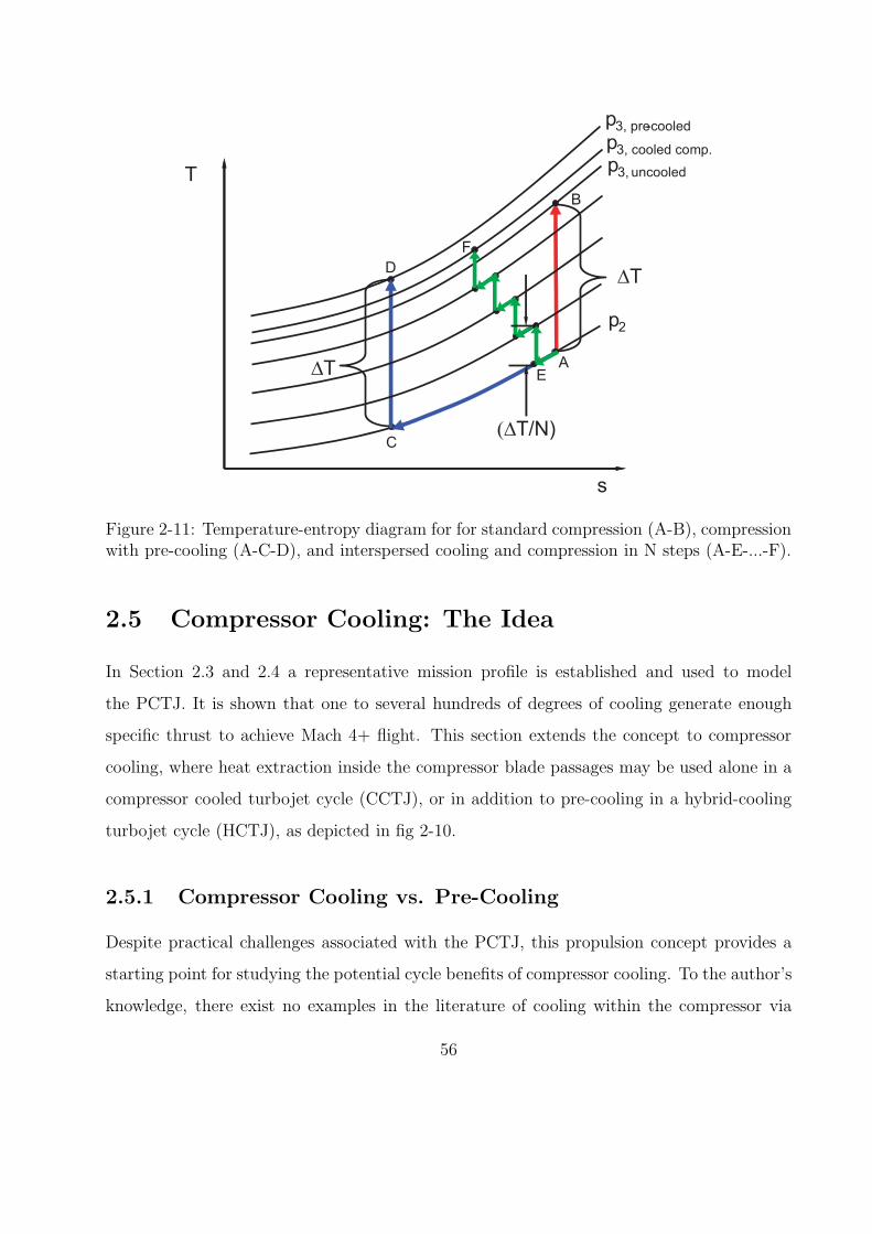
T
s
∆T
∆T
p2
p3, uncooled
p3, pre-cooled
A
B
C
D
p3, cooled comp.
E
F
(∆T/N)
Figure 2-11: Temperature-entropy diagram for for standard compression (A-B), compressionwith pre-cooling (A-C-D), and interspersed cooling and compression in N steps (A-E-...-F).
2.5 Compressor Cooling: The Idea
In Section 2.3 and 2.4 a representative mission profile is established and used to model
the PCTJ. It is shown that one to several hundreds of degrees of cooling generate enough
specific thrust to achieve Mach 4+ flight. This section extends the concept to compressor
cooling, where heat extraction inside the compressor blade passages may be used alone in a
compressor cooled turbojet cycle (CCTJ), or in addition to pre-cooling in a hybrid-cooling
turbojet cycle (HCTJ), as depicted in fig 2-10.
2.5.1 Compressor Cooling vs. Pre-Cooling
Despite practical challenges associated with the PCTJ, this propulsion concept provides a
starting point for studying the potential cycle benefits of compressor cooling. To the author’s
knowledge, there exist no examples in the literature of cooling within the compressor via
56

blade passage surface heat extraction. It is first necessary, then, to compare the concept of
the PCTJ to compressor cooling. The temperature-entropy diagram in Fig. 2-11 compares
standard ideal compression (A-B) to constant pressure pre-cooling (A-C) followed by isen-
tropic compression (C-D). The comparison is made on an equal work basis, meaning ∆T
is the same for the isentropic compression process in both cases (a perfect gas is assumed).
Process (A-E-...-F) superimposes a third conceptualization, the case of N constant-pressure
cooling steps interspersed with N equal work steps. It is implied by the temperature rise of
∆T/N that the total compression work for all three processes (A-B), (A-C-D), (A-E-...-F)
is equal. It is argued by the author that process (A-E-...-F) could represent: (1) an N stage
compressor with constant-pressure cooling in an inlet guide vane and the first N-1 stators,
or (2) perhaps, in the limit as N approaches infinity, a single stage device with a continuous
cooling scheme. Both descriptions are generally referred to as cooled compressors.
Under the perfect gas assumption, two lines of constant-pressure diverge on a T-s diagram
with increasing temperature or entropy. The implication of this fact on the three processes
shown is that the theoretical pressure rise capability of the pre-cooled compressor is greatest,
followed by the cooled compressor (schematically similar to intercooling), and finally the
standard (adiabatic) compressor, because compression work done at a lower temperature
results in greater pressure rise. This idealized model fails, however, to account for the fact
that a real pre-cooler may create significant loss of stagnation pressure [29, 66], and that
cooling within blade passage surfaces may have additional aerodynamic benefit. Assuming
that a cooled compressor introduces no new gas path geometry, and hence no new loss
generating solid boundaries, the cooled compressor underperformance may be mitigated or
even reversed when compared to a real pre-cooler2.
The natural point of departure from this conceptual example is to determine in what
situations a cooled compressor has comparable effect to a pre-cooled compressor with real
pressure loss. Figure 2-12 depicts two additional processes superimposed on the previous
2In addition to the loss penalties associated with a real pre-cooler, significant system weight penaltiesfrom heat exchanger hardware are also seen as a technological challenge, requiring lightweight heat exchangermaterials to be surmounted [66]. This thesis does not address the modeling of system weight. It would benecessary in any vehicle-system level study.
57

T
s
∆Tcomp
p2
p3, uncooled
p3, pre-cooled
A
B
C
D
p3, cooled comp.
E
F
(∆T/N)C'
D'
∆Tcomp
B'
∆Tcool
∆Tcool
Figure 2-12: Same as Fig 2-11 with real precooled compression process (A-C′-D′) and com-pression followed by constant pressure post-cooling (A-B-B′).
temperature-entropy diagram. Process (A-C′-D′) represents a pre-cooling with loss of pres-
sure followed by an isentropic compression with the same work input as process (A-C-D).
Compared to this is an isentropic compression followed by constant pressure cooling, a so-
called post-cooling process (A-B-B′). It is argued by the author that the constant pressure
post-cooling is a conservative limiting case of a cooled compressor that assumes no additional
total pressure losses because no new gas path geometry is introduced.
One source suggests typical pre-cooler stagnation pressure loss (∆pt/pt) of one to eight
percent, with loss being a function of pre-cooler temperature drop [66]. Figure 2-13 shows the
critical pre-cooler recovery factor versus non-dimensional heat addition for the comparison
of two isentropic compressors with pressure ratios of 2, 5, and 8. The first device follows
process (A-C′-D′) in Fig. 2-12, i.e., isentropic compression preceded by a real pre-cooler
with stagnation pressure recovery of πx, while the second device follows process (A-B-B′),
i.e. isentropic compression followed by a constant pressure cooling process that represents a
58

−0.1 −0.09 −0.08 −0.07 −0.06 −0.05 −0.04 −0.03 −0.02 −0.01 00.9
0.91
0.92
0.93
0.94
0.95
0.96
0.97
0.98
0.99
1
Heat Transfer, q*=(q/cpT
t0)
Pre
−coo
ling
Pre
ssur
e R
ecov
ery,
π x
πc=2
πc=5
πc=8 Pre−cooling favored
Post−cooling favored
Figure 2-13: Critical pre-cooling stagnation pressure recovery vs. cooling load. Operationabove the line favors real pre-cooled compression, while operation below the line favorsa lossless post-cooled compressor (a limiting case of cooled compressor with no new lossgenerating gas path surfaces). Plot is made on an equal work, equal cooling basis for pressureratios of 2, 5, and 8.
conservative limiting case of a cooled compressor. To first order, the presence of compressor
cooling is assumed to introduce no new loss mechanisms. The interpretation of this plot is
that for a given level of cooling, q∗, the pre-cooled compressor is favorable if πx is above the
line, while the post-cooled compressor is favorable if πx is below the line. As the absolute
value of cooling increases, the acceptable pressure recovery for the pre-cooler decreases. For
an inlet total temperature of ∼ 1000K, found near the high speed flight point of M = 4
and 25km altitude, q∗ = −0.1 corresponds to ∼ 100K of cooling, comparable to PCTJ
requirements presented in the analysis of Section 2.4. Thus this simple and conservative
analysis suggests that scenarios may exist for which compressor cooling either in CCTJ or
HCTJ operation is favorable to the PCTJ. In Section 3.6 a heat transfer analysis indicates
59

uu
Given:
uuuuttu ,, T, pV, T, pMuu⇒
dd
Q,, du&
uα
d
Q&
α α
α
ρ
Figure 2-14: Control volume of a diffusing blade passage with heat extraction. Upstreamand downstream flow angles, αu and αd, respectively, are assumed fixed.
that individual blade rows are capable of providing heat transfer rates roughly an order of
magnitude smaller than q∗ = −0.1, suggesting that high-solidity, multistage compressors
with low pressure ratio having cooling in multiple blade rows may be able to achieve heat
transfer rates for similar application as a pre-cooler.
2.5.2 Diffusing Passage Heat Extraction
A one-dimensional, steady control volume (CV) model of a cascade passage with cooling,
as depicted in Fig. 2-14, is performed to study how cooling affects the loading capability of
the blade row. The passage is treated as a subsonic stator, with uniform inflow and outflow
conditions. The upstream Mach number, stagnation pressure, and stagnation temperature
are assumed known. The upstream and downstream flow angles, αu and αd, respectively,
are assumed constant. The dimensionless cooling, q∗, is defined per Equation 2.2. Mass
conservation, axial and circumferential momentum conservation and energy conservation ex-
pressions are applied, along with the ideal gas law. Further, entropy generation is neglected,
60

−0.2 −0.1 0 0.1 0.2
0.4
0.6
0.8
1
q*
Cp
Mu=0.4
Mu=0.6
Mu=0.8
(a) Pressure Coefficient, Cp, vs. heating/cooling,±q∗ in selected stator passage, at various up-stream Mach numbers.
−0.2 −0.1 0 0.1 0.2−0.06
−0.04
−0.02
0
0.02
0.04
0.06
0.08
q*
∆ p
t/ptu
Mu=0.4
Mu=0.6
Mu=0.8
(b) Fractional change in stagnation pressure,ptd−ptu
ptu, vs. heating/cooling, ±q∗ in selected sta-
tor passage, at various upstream Mach numbers.
Figure 2-15: Cooled stator passage control volume model.
and the specific entropy transfer associated with heat extraction is estimated to occur at a
temperature that is the average of the upstream and downstream static temperatures:
strans = sd − su =q
12(Tu + Td)
(2.11)
Solution of the governing equations at three subsonic inlet Mach numbers, with upstream
and downstream flow angles set to αu = 50 and αd = 25, respectively, suggests that cool-
ing increases the dimensionless static pressure rise in the passage, Cp = 2 (pd − pu) /ρuV2u ,
as shown in Figure 2-15(a). As Mu increases, the effect of cooling is greater, as seen by the
relative slopes of the three lines. This result is consistent with the Mach number depen-
dence of the static pressure sensitivity coefficient in quasi one-dimensional flow with heat
transfer [27, 80]. Figure 2-15(b) shows that cooling also increases the passage stagnation
pressure, with heating producing the opposite effect. This is also consistent with the quasi
1-D result, the so-called Rayleigh line. This CV analysis suggests that the loading and total
pressure change benefit from a given amount of heat extraction is an aero-thermodynamic
effect, i.e., it is Mach number dependent. In addition, the CV analysis shows that exit Mach
number and stagnation temperature are lowered by heat extraction. It may be hypothesized
that these effects will provide favorable inlet conditions to downstream blade passages in a
multi-stage compressor.
61

2.5.3 Research Questions
Two high-level research questions may now be posed in the study of compressor cooling:
• What is the aerodynamic/thermodynamic performance effect of heat extraction within
the blade passages?
• How should the presence of cooling affect the design of a new compressor?
In this thesis the latter question is not directly addressed. The focus remains on the
first question, i.e., the aerodynamic and thermodynamic benefits of compressor cooling on
a device with an adiabatic design point. The following detailed research questions are thus
addressed in Chapter 3:
• What is the effect of surface heat extraction on blade-to-blade performance within the
compressor?
• How does cooling change the generation of entropy within the blade passage?
• How does cooling affect the performance of a multi-stage axial compressor in terms of
conventional metrics of pressure ratio, π, corrected mass flow, mc, and efficiency, η?
• What are the best efficiency metrics for this type of device?
2.5.4 Challenges and Unknowns
A key challenge in the assessment of compressor cooling is the development of a new modeling
framework to account for the level of heat extraction. Blade passage performance with heat
extraction must be defined in terms of conventional parameters, plus a new cooling parame-
ter. In addition, conventional efficiency metrics and figures of merit must be reconsidered in
light of the new cooling variables.
The unknowns associated with compressor cooling include the effect of heat extraction on
the bulk flow through blade passages, and the subsequent effect at the multistage compressor
level. The effect of location of heat extraction within the multistage compressor is also an
important unknown that this research must address.
62

2.6 Chapter Summary
This chapter provides a review of the challenges associated with versatile turbopropulsion
systems for low-to-high Mach number flight, to motivate the idea of compressor cooling.
Inlet stagnation temperature rise with increasing flight Mach number along a mission trajec-
tory limits the production of thrust by limiting heat addition capability in the combustor.
Compressor cooling, like pre-cooling, is expected to improve cycle performance and hardware
durability. Preliminary analysis suggests that compressor cooling, in exclusive operation or
in hybrid operation with a pre-cooler may be favorable to the pre-cooled turbojet in certain
scenarios. The hypothesized benefits of compressor cooling are summarized below:
• Thermodynamic benefit of compression at colder temperatures.
• Operability benefit associated with greater mass flow ingestion.
• Aerodynamic benefit associated with increased loading across compressor blade pas-
sages, potentially enabling a more compact design.
• An efficiency benefit versus a pre-cooler, as no new gas path surface geometry is intro-
duced. In hybrid operation compressor cooling may reduce the surface area require-
ments of a pre-cooler.
• Improved durability, especially in the rear of the compressor, through material tem-
perature reduction.
The next chapter explores the component performance aspects of compressor cooling in
greater detail, using computational experiments and meanline modeling. Emphasis is placed
on blade passage flows with heat extraction and the cooled compressor as a component alone.
63

64

Chapter 3
Compressor Cooling: A Novel
Turbomachinery Concept for Mission
1
Chapter 2 introduces the concept of compressor cooling, a novel approach to improving
axial compressor performance and extending the flight envelope of a high speed propulsion
system. A mission analysis of a pre-cooled turbojet (PCTJ) cycle suggests that several
tens to hundreds of degrees Kelvin of pre-cooling can stretch the operating envelope of a
conventional turbopropulsion system to Mach 4+. Compressor cooling in a turbojet cycle is
an offshoot of the PCTJ concept, that may be an enabler to high speed flight–independently
or in tandem with pre-cooling.
This chapter presents the first description of the expected performance of a single and
a multistage cooled axial compressor, through computational experiments and meanline
modeling. Results suggest that for an axial compressor with an adiabatic design point,
compressor cooling would: 1) raise the overall pressure ratio (at a given corrected flow),
2) raise the maximum mass flow capability, 3) raise the efficiency, defined as the ratio of
isentropic work for a given pressure ratio to actual shaft work, and 4) provide rear stage
choking relief at low corrected speed. In addition, a given amount of cooling is found to have
65

more impact in the front stages versus the rear stages. This is primarily a thermodynamic
effect that results from the fact that, for a given gas, the compression work required to achieve
a given pressure ratio decreases as the gas becomes colder. For an eight-stage compressor
with an adiabatic design pressure ratio of 5, heat extraction equal to 1% of inlet stagnation
enthalpy flux in the first four blade rows is found to improve pressure ratio and efficiency
by 23% and 12%, respectively, at design values of corrected speed and corrected mass flow.
Choking mass flow at design speed is also found to improve by 5%.
The end of the chapter discusses heat transfer considerations that set performance limits,
and discusses the appropriate selection of efficiency metrics for non-adiabatic compressors.
The heat transfer considerations indicate that the engineering challenges lie in achieving high
enough heat transfer rates to provide significant impact to the compressor’s performance.
3.1 Objectives
The research question that must be answered is how blade passage cooling affects the per-
formance of a multistage compressor. It is hypothesized that blade passage cooling has
both thermodynamic and aerodynamic benefits that lead to improvements in multistage ax-
ial compressor performance and operability. Testing this hypothesis requires meeting the
following objectives:
1. Describing the bulk effect of surface heat extraction on the performance of diffusing
blade passages typical of axial compressors.
2. Characterizing the on- and off-design performance and operability of a single- or multi-
stage compressor with cooled blade passages utilizing different cooling schemes.
3. Estimating the available heat transfer potential in axial compressors.
4. Quantifying the relative importance of the thermal and viscous dissipation loss mecha-
nisms and defining an appropriate cooled compressor efficiency metric at the component
and system level.
66

3.2 Technical Approach
Concept 1:
Compressor Cooling
2D Blade Passage Flows
On- and off-design
Meanline Analysis Geometries of
Practical InterestNASA Rotor 35 3D CFD
2D Linear Cascade CFD
with Heat Extraction
Heat transfer BC
Wall Temperature BC
Generic
Performance
‘Rules’
Bulk Performance Metrics
Loss, Turning
Exit Conditions
Entropy Generation
Viscous Diffusion
Thermal Diffusion
Single Stage Multi-StageStage Matching
Effects
Heat Transfer
CapabilityReynolds Flat
Plate Analogy
Efficiciency MetricsAdiabatic Ref. Process
Non-adiabatic Ref. process
Figure 3-1: Compressor cooling technical road map.
The research objectives are met through computational experiments on blade passage
flows with heat extraction, coupled with on- and off-design cooled compressor meanline
analysis. The final step involves estimating the limits imposed by the heat transfer capability
of blade passages. A technical road map of the compressor cooling study is shown in Figure 3-
1. The technical approach is executed sequentially in the remaining sections, as described
here.
Results from computational fluid dynamics (CFD) modeling of typical two-dimensional
diffusing blade passages (linear cascades) with heat extraction are presented in section 3.3.
The heat transfer-incidence design space of two representative cascade geometries is mapped
in terms of typical bulk performance metrics in Section 3.3.2. The two entropy generation
67

mechanisms, viscous and thermal diffusion, are also quantified in Section 3.3.3. The bulk
performance figures of merit lead to generic rules for cooled blade passages, presented in
Section 3.3.4.
In section 3.4, these rules are applied to the on- and off-design meanline analyses of a
single- and eight-stage compressor with low pressure ratio and an adiabatic design point.
Pressure ratio and efficiency maps are thus generated, and the off-design behavior is de-
scribed in terms of incidences and losses in individual stages. The meanline analysis shows
improvements in pressure ratio, mass flow, and efficiency, and indicates that cooling pro-
duces rear stage choking relief. In addition, it is found that a given amount of cooling has
the greatest effect if implemented in the front of the device.
In section 3.5, a CFD computation on a three dimensional rotor with and without cooling
is presented. Cooling improvements are shown to be in accord with meanline predictions,
suggesting compressor cooling as a concept is applicable to geometries of practical interest. It
is indirectly inferred that the pressure rise from cooling is primarily an aero-thermodynamic
effect, whereas the mass flow increase is a purely thermodynamic effect.
In section 3.6 heat transfer considerations are taken up. A simple model using Reynolds
analogy on a flat plate is invoked to demonstrate that the limitations to cooled compressor
performance come from available heat transfer areas. It is also pointed out that available
heat transfer would be greatest in the rear of a compressor, which competes with the finding
that the greatest effect comes from cooling in the front.
In section 3.7, two efficiency metrics for non-adiabatic compressors are discussed. The
first metric, used throughout the thesis, compares the actual performance to an adiabatic
reference process. The second metric compares the actual performance to a non-adiabatic
reference process. It is argued that the first metric is appropriate for comparing the output
between adiabatic and non-adiabatic compressors at the component level, while the second
metric may be more appropriate as part of a system level analysis.
68
3.3 Blade Passage Flows with Heat Extraction
Computational experiments of two representative cascade geometries with and without cool-
ing are presented in this section. Results given in terms of bulk aerodynamic performance
metrics show that cooling improves cascade performance by reducing total pressure drop
and by increasing turning. Bookkeeping of entropy generation and entropy flux in the com-
putations reveals that the total pressure reduction coefficient is driven by both viscous and
thermal diffusion. Viscous diffusion is found to have strong Mach number dependency and
weak dependency upon heat transfer boundary conditions, whereas the opposite is found to
be true of thermal diffusion.
3.3.1 Cascade Cases
Two-dimensional CFD experiments using Fluent are performed on two different cascade
geometries in order to produce bulk aerodynamic performance figures of merit. The two
selected geometries are representative of airfoils used in multistage compressors. Cascade 1
is based on a NACA 65 airfoil series blade definition, with an inlet and exit metal angle of
χin = 38 and χout = 0, respectively, and a cascade solidity of 0.75. Cascade 2 has χin = 51,
χout = 14, and solidity of 1.0, similar to the mid span metal angles of the NASA/GE E3
compressor.
Geometry and Computational Domain
Figure 3-2 shows the gridded computational domains, as well as enlarged airfoil region views,
for cascades 1 and 2. Cascade 1 has ∼ 6000 grid cells. Grid y+ is ∼ 5−10 in the wall adjacent
cells, with Reynolds number based on chord (Rec) in the range of 100, 000 to 200, 000. The
computational domain extends one axial chordlength upstream of the leading edge and two
axial chordlengths downstream of the trailing edge. Cascade 2 has ∼ 26000 grid cells. Grid
y+ is ∼ 1 − 3 in the wall adjacent cells, with Rec in the range of 300, 000 to 500, 000. The
computational domain extends two axial chordlengths upstream of the leading edge and
three axial chordlengths downstream of the trailing edge.
69

(a) Cascade 1 computational grid. (b) Cascade 1 grid around airfoil.
(c) Cascade 2 computational grid. (d) Cascade 2 grid around airfoil.
Figure 3-2: Computational grids for cascades 1 and 2.
Both blade passage geometries are modeled in Fluent using the k− ǫ turbulence models.
The near wall region is modeled using an enhanced wall treatment, which smoothly switches
between: 1) completely resolving the viscous sublayer in the near wall region and 2) a
wall function that bridges the viscous sublayer and the fully turbulent region using a semi-
empirical function, depending upon the value of y+ adjacent to any solid boundaries. The
enhanced wall treatment resolves the viscous sublayer when the y+ value of the first wall
adjacent cell is ∼ 4 − 5 [23]. Thus the cascade 1 boundary layer is generally defined using
wall functions, while cascade 2 has a generally resolved viscous sublayer1.
1Although grid resolution, selection of turbulence model, and level of inlet turbulence have some effecton overall bulk performance levels, they are found to not affect trends between adiabatic and cooled bulk
70

For both cascades, matrices of cases are assembled by varying the flow inlet angle and
the ratio of upstream total pressure to downstream static pressure. For cascade 1, cases are
generated using (1) adiabatic wall and (2) constant heat flux boundary conditions (BCs).
For cascade 2, cases are generated using (1) adiabatic wall and (2) cooled wall temperature
BCs equal to one-half the freestream value. The non-dimensional cooling rate is defined as
the heat removed from the flow normalized by the inlet stagnation enthalpy flux,
q∗ =Q
mht,in
=∆ht
ht,in
=∆Tt
Tt,in
< 0 (for cooling). (3.1)
Post-processing
Integrated bulk flow properties are area- or mass- averaged one chord length upstream of the
airfoil leading edge (inlet) and one chord length downstream of the trailing edge (outlet). For
example, velocities are mass-averaged, while pressures are area-averaged2. All of the results
are interpolated to a given set of inlet Mach numbers in order to produce bulk performance
data. The primary figures of merit used to characterize bulk blade passage performance
are non-dimensional total pressure reduction (loss buckets3), ω, and deviation (difference
between air and blade metal exit angle), δ, defined as
ω =pt,in − pt,out
pt,in − pin(3.2)
and
δ = βout − χout. (3.3)
Results in the next section are either presented at constant dimensionless cooling rate, q∗,
or constant wall temperature ratio, Twall/Tt,in.
performance.2It is found that the differences between area-averaging and mass-averaging are not appreciable in terms
of the essential conclusions of the thesis.3Strictly speaking, the term loss bucket should be used with adiabatic blade-to-blade flows only, as in
these flows entropy generation (lost work) is tied to loss of total pressure alone. Here, the term loss bucketis used per its conventional definition of total pressure reduction divided by inlet dynamic head.
71

3.3.2 Bulk Performance
The computations reveal that cooling impacts blade passage flows in the following ways:
1. For a given value of q∗ at a given inlet Mach number, cooling improves performance
by producing a relatively uniform reduction in ω across the loss bucket.
2. For a given value of q∗ the reduction in ω increases as inlet Mach number increases.
3. The effect of reversible cooling on a one-dimensional channel flow4 provides a reasonable
first approximation to the effect of cooling on total pressure change at low inlet Mach
numbers, whereas at high subsonic inlet Mach numbers (e.g., Min ∼ 0.8), cooling
appears to have a more beneficial impact above and beyond the bulk cooling of the
working fluid.
4. Cooling increases the flow turning (or lowers δ). Table 3.1 summarizes the average
level of change of flow turning for cascade 1, for q∗ = −0.001.
5. Cooling reduces the exit Mach number5. The effect of a Mach number reduction
downstream (in most compressors) will be to reduce the inlet Mach number into the
next blade row, thereby potentially reducing losses associated with locally supersonic
regions on the blade.
6. Cooling decreases the exit stagnation temperature. This has a favorable effect on the
downstream blade rows, as less work is required to compress colder air to a given
pressure ratio.
4see Equation 3.55see Equation 3.6
Min ∆βna = −∆δna
0.4 0.1
0.8 0.25
Table 3.1: Average effect of q∗ = −0.001 on flow turning for cascade 1, across a range ofincidences.
72

15 20 25 30 35 400
0.02
0.04
0.06
0.08
0.1
0.12
0.14
0.16
Tot
al P
ress
ure
Loss
Coe
ffici
ent,
ω=∆
pt/(
pt,i
n−p
in)
Flow Inlet Angle, βin
Min
=0.8
Min
=0.4
Adiabatic
Cooled, q*=−0.001
(a) Solid lines are adiabatic wall BC; dashed lines are q∗ = qht,in
= −0.001.
34 36 38 40 42 44 46 48 50 52 54 560
0.02
0.04
0.06
0.08
0.1
0.12
0.14
0.16
Loss
, ω
=∆p
t/(p
t,in
−pin
)
Flow Inlet Angle, βin
Min
=0.8 Min
=0.4
Adiabatic
Cooled, Twall
/Tt,in
=0.5
(b) Solid lines are adiabatic wall BC; dashed lines are Twall/Tt,in = 0.5.
Figure 3-3: Total pressure reduction coefficient, ω, vs. flow inlet angle, βin, at low (0.4) andhigh (0.8) inlet Mach number, for cascades 1 and 2.
73

34 36 38 40 42 44 46 48 50 52 54 56−0.01
−0.009
−0.008
−0.007
−0.006
−0.005
−0.004
−0.003
−0.002
−0.001
0N
on−D
imen
sion
al c
oolin
g, q
*=∆h
t/ht,i
n
Flow Inlet Angle, βin
Min
=0.8
Min
=0.4
Figure 3-4: Non-dimensional cooling, q∗, vs. flow inlet angle, βin, at low (0.4) and high (0.8)inlet Mach number, for cascade 2 with Twall/Tt,in = 0.5 cooling boundary condition.
Figure 3-3 shows the adiabatic and cooling wall BC loss bucket for cascades 1 (q∗ =
−0.001) and 2 (Twall/Tt,in = 0.5), respectively, at a low (0.4) and high (0.8) Mach number.
For a given cooling wall temperature or heat flux BC at a fixed Mach number, there is a fairly
uniform reduction in ω across the range of operational cascade inlet angles. Corresponding
values of q∗ for cascade 2 with Twall/Tt,in = 0.5 are shown in Figure 3-4. As q∗ shows a
relatively slight variation with incidence at a given Mach number, one may conclude that
this uniform ω reduction is consistent with observation 1. It is also apparent that the
reduction in ω at a given wall temperature ratio or q∗ increases with increasing inlet Mach
number. In the fixed wall temperature case (cascade 2) absolute values of q∗ are lower at
the higher Mach number, implying that the benefit from cooling at a fixed q∗ is further
pronounced with increasing Mach number.
74

10 15 20 25 30 35 40 45−1.8
−1.6
−1.4
−1.2
−1
−0.8
−0.6
−0.4
−0.2
0
Sen
sitiv
ity C
oeffi
cien
t
Flow Inlet Angle, βin
Min
=0.4
Min
=0.6
Min
=0.8
Computed
−γMin
2/2
(a) Cascade 1.
30 35 40 45 50 55 60−1.8
−1.6
−1.4
−1.2
−1
−0.8
−0.6
−0.4
−0.2
0
Flow Inlet Angle, βin
Sen
sitiv
ity C
oeffi
cien
t
Computed
−γMin
2/2
Min
=0.4
Min
=0.6
Min
=0.8
(b) Cascade 2.
Figure 3-5: CFD estimated (solid, Equation 3.4) vs. analytical one dimensional channel flowsensitivity coefficient (dashed, Equation 3.5). Data normalized to q∗ = q/ht,in = −0.001.
75

To elaborate on observation 3, an estimate of the fractional change in total pressure for a
given amount of dimensionless cooling is obtained by comparing adiabatic and non-adiabatic
CFD computations at identical inlet Mach numbers:
(∂pt
pt
∂Tt
Tt
)
M=constant
≈
(∆pt,cool
pt− ∆pt,ad
pt
)
∆Tt,cool
Tt
. (3.4)
The computed values given by Equation 3.4 may be compared to an analytically derived one
dimensional channel flow value using the sensitivity coefficient [80] for the cooled cases, i.e.,
dpt
pt= −γM
2
2
dTt
Tt≈ −γM
2in
2q∗ (|q∗| ≪ 1) . (3.5)
Figure 3-5 demonstrates that at low Mach number the effect of cooling on total pressure
reduction is well predicted by the analytical result given in Equation 3.5. This can be
interpreted as the aero-thermodynamic benefit of heat extraction in a blade passage. At
high Mach number the total pressure reduction is greater for the computed flow fields,
indicating a potential additional aerodynamic benefit.
Observation 5 indicates that cooling reduces the exit Mach number of the cascade flow.
This result is demonstrated by Figure 3-6. The exit Mach number reduction increases with
increasing inlet Mach number, consistent with the influence coefficient from one dimensional
compressible channel flow [27, 80],
dM2
M2=
(1 + γM2)(1 + γ−12M2)
1 −M2
dTt
Tt− 2(1 + γ−1
2M2)
1 −M2
dA
A. (3.6)
From the expression in Equation 3.6, it is clear that subsonic cooling has the effect of
directly reducing the Mach number (just as heating does the opposite, driving flow toward
sonic conditions) by reducing the total temperature, and indirectly reducing the Mach num-
ber by an increase in effective exit flow area caused by a reduction in deviation.
76

30 35 40 45 50 55 600.2
0.25
0.3
0.35
0.4
0.45
0.5
0.55
Mou
t
Flow Inlet Angle, βin
AdiabaticCooled, T
wall/T
t,in=0.5M
in=0.8
Min
=0.4
Figure 3-6: Adiabatic vs. cooled exit Mach number, Mout, for cascade 2. Solid line withcircles represents adiabatic boundary conditions; dashed line with triangles represents bladesurface cooling. Wall temperature BC is Twall/Tt,in = 0.5.
3.3.3 Entropy Generation
Observation 3 in the previous subsection indicates that the reduction in ω from cooling occurs
both from aero-thermodynamic compressibility effects (reversible cooling) and from the re-
balancing of entropy generation (loss) inside the flow field with entropy removal across blade
surfaces. The constant wall temperature BCs on the airfoil surfaces of cascade 2 allow for
easy computation of the entropy flux across the blades themselves. From this, it is possible
to compute the entropy generation, by considering the second law of thermodynamics over
the computational domain, namely,
sgen
cp=sout − sin
cp− q∗
Tt,in
Twall=sout − sin
cp− ht,out − ht,in
cpTwall. (3.7)
The entropy generation is comprised of two components, viscous dissipation and ther-
77

mal dissipation[27], which may also be computed by numerical integration over the entire
computational domain,
sgen
cp=
1
mcp
∫∫∫
V
1
Tτik
(∂ui
∂xk
)
︸ ︷︷ ︸
viscous
+k
T 2
(∂T
∂xi
∂T
∂xi
)
︸ ︷︷ ︸
thermal
dV, (3.8)
where,
τik = λ∂ul
∂xlδik + µ
(∂ui
∂xk+∂uk
∂xi
)
(3.9)
and the factor λ is assumed to be equal to −23µ [77]. It is important to note that in order to
use equations 3.8 and 3.9 to calculate the specific entropy generation for turbulent flows, it
is appropriate to use the effective viscosity, µ (and effective thermal conductivity, k), which
is the sum of the laminar and turbulent, or eddy, viscosities (and thermal conductivities).
Figure 3-7 demonstrates that it is possible to re-construct the entropy generation using
both the technique of entropy flux bookkeeping given by Equation 3.7 and the direct inte-
gration of the viscous and thermal dissipation terms given by Equation 3.8. The figure also
demonstrates that entropy generation is greater for the cooled cases versus the adiabatic
cases. The net decrease in ω from cooling shown in Figure 3-3 must therefore occur because
the transfer of entropy across the blade surface counters additional entropy generation by
thermal dissipation, such that the exit total pressure is higher in the cold wall case than for
the adiabatic cascade. Specifically, the entropy constitutive relation for a perfect gas,
sout − sin
cp= ln
Tt,out
Tt,in− γ − 1
γlnpt,out
pt,in=sgen
cp+ q∗
Tt,in
Twall, (3.10)
may be used to manipulate the definition of ω:
ω =pt,in − pt,out
pt,in − pi
=1 −
[
(1 + q∗) exp(
−q∗ Tt,in
Twall− sgen
cp
)] γγ−1
1 −[1 + γ−1
2M2
in
] γ1−γ
. (3.11)
78

30 35 40 45 50 55 600
0.002
0.004
0.006
0.008
0.01
0.012
0.014
0.016
0.018
s gen/c
p
Flow Inlet Angle, βin
Tw
/Tt,in
=0.5M
in=0.8
Tw
/Tt,in
=0.5,M
in=0.4
adiabatic M
in=0.8
adiabatic M
in=0.4
Figure 3-7: Cascade 2, computed entropy generation vs. incidence at low (0.4) and high (0.8)inlet Mach number using net entropy flux method (solid lines given by Equation 3.7) anddirect volume integration(dashed lines given by Equation 3.8). Adiabatic (red) and cooled(blue, Twall/Tt,in = 0.5) cases shown.
The numerator of the right hand side of Equation 3.11 shows that ω is affected both by the
temperature reduction from cooling (the 1 + q∗ term), and the competition between entropy
transfer and entropy generation in the exponential (q∗ < 0 for cooling).
Figure 3-8 presents bar charts of the viscous and thermal dissipation at a low (0.4) and
high (0.8) inlet Mach number, for both the adiabatic and wall temperature boundary condi-
tion cases. From these charts several interesting observations follow. First, in the adiabatic
cases virtually all of the entropy generation comes from viscous dissipation. Second, in the
cases with Twall/Tt,in = 0.5, the relative magnitudes of viscous and thermal dissipation are
highly Mach number dependent. At low Mach numbers, thermal dissipation is the larger
contributor to total entropy generation, whereas at high Mach number viscous dissipation is
the larger contributor. The results show that viscous dissipation has a strong Mach number
79

30 40 50 600
0.005
0.01
0.015
Adiabatic
s gen/c
p
30 40 50 600
0.005
0.01
0.015
Twall
/Tt,in
=0.5
30 40 50 600
0.005
0.01
0.015
s gen/c
p
Flow Inlet Angle, βin
30 40 50 600
0.005
0.01
0.015
Flow Inlet Angle, βin
Min
=0.4 Min
=0.4
Min
=0.8 Min
=0.8
Viscous
Thermal
Figure 3-8: Cascade 2, viscous (black), and thermal (gray) dissipation vs. incidence at low(0.4) and high (0.8) inlet Mach number. Plots on left are adiabatic wall BC; plots on rightare Twall/Tt,in = 0.5.
dependency, but is virtually independent of the cooling BC, whereas thermal dissipation has
weak Mach number dependency but is, of course, highly dependent upon the wall tempera-
ture BC. Since the viscous dissipation term is dependent upon local strain rates in the flow
field, this may suggest that the velocity boundary layer is fairly independent of the temper-
ature boundary layer. This implies that a simple model for the effect of blade surface heat
extraction on blade passage aerodynamic performance could be constructed by building two
separate models for the viscous and thermal dissipation, where the viscous dissipation could
come strictly from adiabatic computations.
In summary, blade passage flows are described by traditional bulk figures of merit such as
ω and δ, as well as by considering the flow from a second law of thermodynamics perspective,
for two different blade passage geometries. The effect of cooling is found to decrease the value
80

of ω and δ, both of which favorably affect compressor performance. In addition, one would
expect that the decrease in the exit stagnation temperature and exit Mach number should
both favorably affect subsequent downstream blade rows, due to the increased pressure rise
capability on a relatively colder fluid and the decrease in ω with decreasing Mach num-
ber. Finally, the loss generation mechanisms in the flowfield, namely viscous and thermal
dissipation, are found to be relatively uncoupled, which indicates that a simple model for
aerodynamic performance of non-adiabatic blade passage flows could be constructed using
these components as the basis.
3.3.4 Generic Rules for Blade Passage Loss and Deviation
Generic rules for ω and δ are next created by postprocessing the CFD results shown in the
previous section. The motivation for using generic rules comes from the fact that no detailed
geometry information exists during the preliminary design of a compressor. These rules serve
as a set of trends that can be used in a preliminary design.
By introducing cooling to the cascades, an additional performance variable is required,
namely, the non dimensional cooling, q∗. For the meanline model in section 3.4, it is assumed
that cooling takes place at a uniform rate over the airfoil surface. In fact, the details of the
cooling distribution could also be a design variable. However, to make use of the data in
a general sense, the definition is simplified to isolate the effect of each variable. The set of
variables that describe the cascade performance parameters of interest are then,
Cascade Performance = f(geometry, i,Min, Rec, q∗), (3.12)
where,
geometry (including airfoil shape and cascade solidity, σ) is fixed for the experiment.
i is the inlet flow incidence angle.
Min is the inlet Mach number.
81

Rec is the inlet Reynolds Number, using airfoil chord as an appropriate length scale.
q∗ is the non-dimensional cooling rate, defined as the ratio of the change in stagnation
enthalpy due to cooling to the inlet stagnation enthalpy (see Equation 3.1). Because
cooling involves heat removal, the adopted sign convention makes q∗ a negative number
for cooled cascades.
For the situation where dependence on Rec is weak6, and the solidity only appears in the
expression for ‘base’ deviation (i.e., Carter’s rule7), Equation 3.12 simplifies to
ω,∆δ = f(i,Min, q∗), (3.13)
where,
ω is the total pressure reduction coefficient.
∆δ is the change in deviation relative to the ‘base’ deviation.
For a low level of cooling (|q∗| ≪ 1), the channel flow sensitivity coefficient relating a
differential change in stagnation temperature of a perfect gas to the resultant differential
change in stagnation pressure is linear for a given Mach number (Equation 3.5). Thus, it is
assumed that to first order, it will be reasonable to scale the observed changes in ω linearly
with the cooling rate.
Generic loss buckets are developed by taking each loss bucket from the CFD data for
cascade 1 and referencing its minimum ω value as ‘zero’ incidence. Polynomial fits are used
to define the bucket in the incidence range of −15 to 15, as shown in Figure 3-9.
6For cascade 1, values of Rec range from 100,000 to 200,000. For cascade 2 Rec values range from 300,000to 500,000. Rec does not change appreciably between comparable adiabatic and cooled cases.
7Carter’s rule gives the base deviation (predominantly a potential flow effect) near the minimum ω point,δbase = mθσ−n, where m is an empirical constant which depends on geometry, θ is the camber angle (angulardifference between blade metal inlet tangency and exit tangency) and n is usually taken as 0.5 for deceleratingcascades [14].
82

−15 −10 −5 0 5 10 150
0.05
0.1
0.15
0.2
0.25T
otal
Pre
ssur
e Lo
ss C
oeffi
cien
t, ω
=∆p
t/(p
t,in
−pin
)
Flow Incidence Angle, i
Min
=0.8
Min
=0.6
Min
=0.4
Adiabatic
Cooled, q*=−0.001
Figure 3-9: Generic adiabatic vs. cooled loss buckets derived from cascade 1 performance.Solid line with circles represents adiabatic boundary conditions; dashed line with trianglesrepresents blade surface cooling. Non-dimensional cooling rate is q∗ = q
ht,in= −0.001.
Nominal deviation for adiabatic cascades at design (minimum ω) is predicted using Carter’s
rule. The deviation is then modified for incidence, Mach number, and cooling rate. The first
deviation modification, ∆δa, is the increase in deviation due to ‘off-design’ incidence and
Mach number for an adiabatic cascade. Figure 3-10 presents a smooth curve fit at three
Mach numbers of ∆δa used in the generic model. The figure demonstrates that the narrow
operability at high Mach number occurs from a rapid deviation increase associated with flow
separation and unrealized flow turning. The physical mechanism that causes the boundary
layer to separate at high Mach numbers is an adverse pressure gradient created by a local
normal shock on the suction side.
The second modification is reduction of deviation due to cooling, ∆δna. The generic
non-adiabatic deviation reduction model is based on the cascade 1 observations summarized
83

−15 −10 −5 0 5 10 15−5
0
5
10
15
20
25
30
Flow Incidence Angle, i
Dev
iatio
n In
crea
se,
∆δa
Min
=0.8
Min
=0.6
Min
=0.4
Figure 3-10: Adiabatic change in deviation, ∆δa, (relative to Carter’s rule) for cascade 1.
earlier in Table 3.1. Figure 3-11 demonstrates that cooling reduces the deviation, and that
the effect improves with inlet Mach number. The effect of inlet Mach number on ∆δna is
included in the generic model, while the effect of incidence is neglected by averaging the
values of ∆δna at each Mach number, as shown by the two solid lines.
The changes in deviation due to cooling do not have as simple an analog as changes in pt,
and hence changes in ω. In this study it is assumed that the observed changes in deviation
due to cooling will scale linearly for cooling rates up to q∗ = −0.01. This model is a significant
simplification of the physical effect, but it is nonetheless valuable to include deviation effects
to give a sense of the potential impact of cooling on axial compressor performance. If levels
of cooling such as this are available (q∗ ∼ −0.01), the model allows for two to three degrees
of deviation to be recovered from the blade rows at high subsonic Mach numbers. Two to
84

5 10 15 20 25 30 35 40 45 500.05
0.1
0.15
0.2
0.25
0.3
Dev
iatio
n R
educ
tion
from
Coo
ling,
∆δ
na
Flow Inlet Angle, βin
Min
=0.8
Min
=0.4
av, Min
=0.8
av, Min
=0.4
Figure 3-11: Additional flow turning from cooling, ∆βcool = −∆δcool, for cascade 1, q∗ =−0.001. Dotted lines with symbols are CFD results. Heavy solid lines are average values(used in meanline analysis) for given inlet Mach numbers.
three degrees of deviation reduction per blade row would make cooling a legitimate control
variable to improve off design matching. In the meanline analysis of the next section, cooling
rates up to ten times higher (q∗ = −0.01) are selected, giving extrapolated turning values due
to cooling of two to three degrees in the high Mach number stages of the compressor. The
next section presents a performance map which gives an idea of the impact of the additional
turning from deviation for the cooled, single stage compressor selected in this study.
3.4 On- and Off- Design Meanline Analysis
In this section, results from 2D CFD experiments are used to assess the effect of cooling on
a single stage and an eight stage compressor. As the number of stages increases, off-design
85

0 0.2 0.4 0.6 0.8 1 1.2
−0.2
−0.1
0
0.1
0.2
0.3
0.4
0.5
0.6
0.7
meters
met
ers
Rotors
Stators
Figure 3-12: Eight stage compressor meridional layout. First stage also analyzed as a singlestage fan.
matching becomes more challenging. The presence of cooling affects matching significantly,
both in terms of the propagation of off-design perturbations to velocity triangles and in
terms of total pressure reduction. Results show that constant corrected speed lines (constant
Nc = N/√Tt,in/Tref) on a compressor map are raised relative to their adiabatic counterparts.
Qualitatively, cooling affects low Nc lines differently than high Nc lines. This is primarily
due to the Mach numbers seen by the airfoils at low and high values of Nc. At high values of
Nc (and hence high rotor Mach numbers), there is a very narrow range of incidences in which
the airfoils may operate successfully. There is also an increase of loss with increasing Mach
number. Cooling (1) increases the pressure rise, (2) increases the turning, (3) decreases the
downstream stagnation temperature, and also (4) slightly decreases the downstream Mach
number. Effects (2), (3), and (4) all potentially affect the flow conditions into the next blade
row in a favorable manner.
86

The eight stage compressor is designed by specifying compressor inlet conditions based
on a flight vehicle at 25 km altitude and flight Mach number of 4 (from the mission analysis
of section 2.3), assuming that a lossless inlet exists upstream of the compressor. The overall
pressure ratio at design is taken as 5, with each stage taken to produce the same pressure
ratio, for simplicity. Air is assumed to behave as a perfect gas8 with γ = 1.4. The compressor
is sized for a ‘typical’ high flight Mach number vehicle by specifying an inlet corrected mass
flow9 of 51 kg/s. The hub and tip radii are chosen so as to keep the meanline radius constant
from blade row to blade row. Each stage is designed to return the flow to the axial direction
at the design point, so that the first stage may also be studied as a single stage fan. The
meridional layout of the eight stage compressor is shown in Figure 3-12.
In order to compare various compressor cooling schemes, the local heat extraction is non-
dimensionalized by the compressor face inlet stagnation enthalpy,
q∗comp =Q
mht,in,comp=
∆ ht
ht,in,comp. (3.14)
The subscript ‘comp’ is dropped in the subsequent discussion of compressor cooling, but it
should be noted that the non-dimensionalization follows Equation 3.14. The results from
the single stage and the eight stage compressors are presented in the next two subsections.
3.4.1 Single Stage Fan
The single stage fan map comparing an adiabatic and a cooled fan stage is shown in Figure 3-
13. For a non-dimensional cooling value of q∗ = −0.0025 in both the rotor and stator, results
indicate that the constant corrected speed line on a given adiabatic compressor map moves up
8In general, a variable specific heat thermodynamic model may be more accurate for a high flight Machnumber vehicle in which air enters the compressor at very high temperature. For consistency between themeanline analysis and the CFD computations γ is chosen to be 1.4. No qualitative difference is expectedbetween a variable or fixed specific heat model.
9mc =m√
Tt/Tref
pt/pref, where Tref and pref are standard day conditions.
87

25 30 35 40 45 50 551
1.05
1.1
1.15
1.2
1.25
1.3
Corrected Mass Flow, mc(kg/s)
Ove
rall
Pre
ssur
e R
atio
, π
a
b
c
d
e
f
g h
100% Nc
60% Nc
Adiabatic, q*=0
All Rows, q*=−0.0025
80% Nc
Figure 3-13: Single stage compressor map, with and without cooling. Solid line is adiabatic;Dashed line is q∗ = −0.0025. 100%, 80%, and 60% Nc lines are shown.
in pressure ratio and in mass flow10. Thus, a cooled compressor produces a greater pressure
rise at a given corrected mass flow and corrected speed. In addition, as mc increases along
a given constant Nc line and the line approaches vertical (i.e. choked), a cooled compressor
can pass greater corrected mass flow versus an adiabatic compressor.
The increase in corrected mass flow occurs both at high and low corrected speed, but
a constant value of q∗ affects the corrected speed lines differently. Table 3.2 presents key
blade passage parameters for points a through h in Figure 3-13. At high Nc (points a-d), the
blade passages see higher inlet Mach numbers and thus have a narrower range of operable
incidences, resulting in a greater sensitivity to the beneficial effects of cooling. For example,
at 100% Nc the ‘stall’ side of the speed line shows a greater improvement in pressure ratio for
the same corrected mass flow (point a vs. b), than at 60%Nc (point e vs. f). Examination of
10It should be noted that some of the chosen values of q∗ in both the single stage and multi-stage exampleslead to values of q∗ which require extrapolation of the two-dimensional cascade data presented earlier.
88

Point Min,R Min,S Mout,R Mout,S iR iS ∆δR ∆δS ωR ωS
a 0.941 0.718 0.772 0.669 0.000 0.000 0.370 0.045 0.177 0.099b 0.941 0.701 0.769 0.645 0.000 1.559 0.370 0.300 0.166 0.096c 0.985 0.831 0.845 0.949 -1.919 -5.772 1.382 3.186 0.206 0.187d 0.985 0.793 0.828 0.770 -1.919 -3.372 1.382 1.013 0.191 0.125e 0.537 0.438 0.468 0.423 0.967 -0.704 0.000 -0.229 0.051 0.050f 0.537 0.436 0.469 0.421 0.967 -0.311 0.000 -0.178 0.048 0.046g 0.664 0.656 0.638 0.718 -7.963 -14.661 0.240 1.743 0.111 0.220h 0.664 0.648 0.634 0.693 -7.963 -13.877 0.240 1.347 0.101 0.185
Table 3.2: Key single stage fan map parameters at points a through h, as shown in Figure 3-13. The variables M , i, ∆δ, and ω are Mach number, incidence, deviation change, and totalpressure reduction coefficient, respectively. The subscripts in and out correspond to theinlet and outlet, respectively. The subscripts R and S correspond to the rotor and stator,respectively
the one-dimensional flow properties at the points shown explains why this is so. The 100%
Nc line is in the high subsonic regime, where cooling has a more pronounced impact on ω and
δ than the low subsonic regime that is encountered along the 60% Nc line. Comparison of the
stator inlet and exit Mach numbers of points c (adiabatic) and d (cooled) shows that in the
adiabatic case the stator behaves as a throttle, and is no longer diffusing the flow, whereas
in the cooled case there is much less total pressure reduction and the stator is still diffusing
the flow. The difference in stator incidence at these points varies by only 2.4 degrees, but
since the inlet Mach number is in the high subsonic regime, ω in the cooled stator is 33%
lower than the adiabatic stator. Comparing these two points to their low Nc counterparts,
points g and h, shows that the smaller change in total pressure reduction due to cooling is
a result of less incidence change and lower inlet Mach numbers. Points e and f show even
less change, as their Mach numbers are closer to the low subsonic regime.
Studies on the single stage fan reveal that the improvement in pressure rise capability
seen on the compressor map is attributable to both the increase in stagnation pressure from
cooling (lower ω) and the increased flow turning (lower δ). Figure 3-14 shows the change
in cooled speed lines when the effects on total pressure reduction and flow turning are both
isolated, and when they are both included. For the selected geometry, both of these effects
89
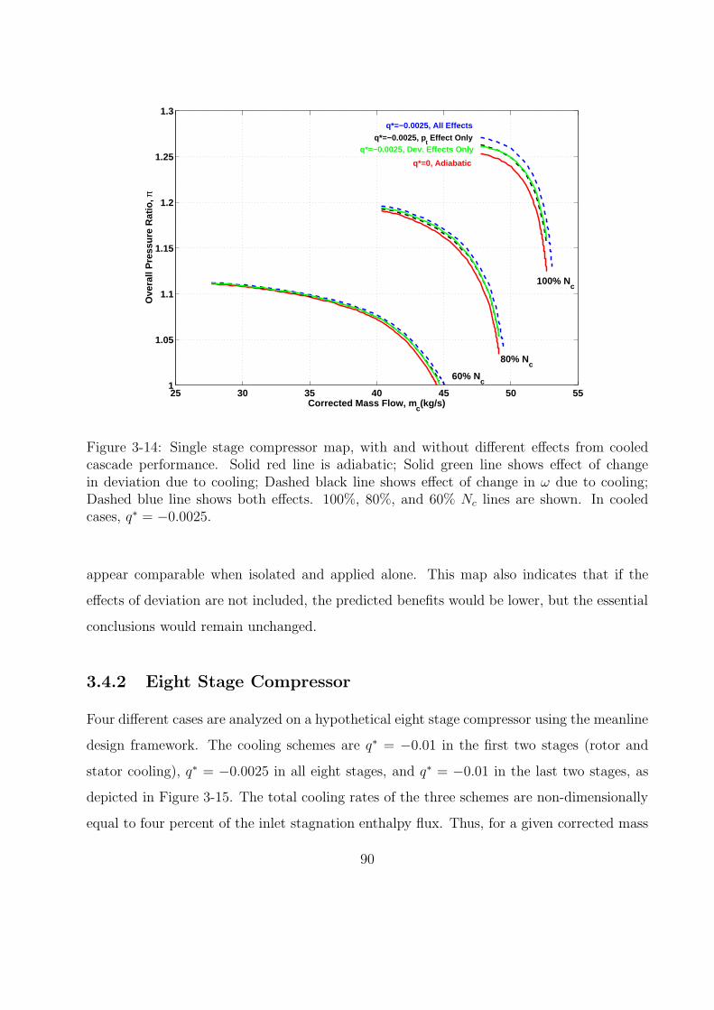
25 30 35 40 45 50 551
1.05
1.1
1.15
1.2
1.25
1.3
Corrected Mass Flow, mc(kg/s)
Ove
rall
Pre
ssur
e R
atio
, π
100% Nc
80% Nc
60% Nc
q*=0, Adiabatic
q*=−0.0025, pt Effect Only
q*=−0.0025, All Effects
q*=−0.0025, Dev. Effects Only
Figure 3-14: Single stage compressor map, with and without different effects from cooledcascade performance. Solid red line is adiabatic; Solid green line shows effect of changein deviation due to cooling; Dashed black line shows effect of change in ω due to cooling;Dashed blue line shows both effects. 100%, 80%, and 60% Nc lines are shown. In cooledcases, q∗ = −0.0025.
appear comparable when isolated and applied alone. This map also indicates that if the
effects of deviation are not included, the predicted benefits would be lower, but the essential
conclusions would remain unchanged.
3.4.2 Eight Stage Compressor
Four different cases are analyzed on a hypothetical eight stage compressor using the meanline
design framework. The cooling schemes are q∗ = −0.01 in the first two stages (rotor and
stator cooling), q∗ = −0.0025 in all eight stages, and q∗ = −0.01 in the last two stages, as
depicted in Figure 3-15. The total cooling rates of the three schemes are non-dimensionally
equal to four percent of the inlet stagnation enthalpy flux. Thus, for a given corrected mass
90

flow and inlet stagnation temperature, the same total cooling rate, in units of power (e.g.
Watts), is extracted from each of the cooled compressors.
Efficiency, η, is defined in Equation 3.15 per the conventional adiabatic efficiency defini-
tion of isentropic work required to achieve a given pressure ratio divided by the actual shaft
work. This constitutes a modification of the conventional definition to account for the effect
of cooling on the change in total temperature (i.e., the temperature ratio alone is no longer
an indicator of shaft work). The use of this efficiency definition allows for the comparison
between the actual work inputs of an adiabatic and a cooled compressor at a given pressure
ratio, because the same adiabatic reference process is assumed in both cases 11.
11An alternate, ‘non-adiabatic’ efficiency (ηna) definition given in section 3.7 compares the actual shaftwork required to achieve given pressure ratio to a lossless, non-adiabatic reference process. The definitionof ηna accounts for the additional theoretically extractable work between the hot gas and cold wall (via ahypothetical heat engine).
0 0.2 0.4 0.6 0.8 1 1.2
0.2
0.1
0
0.1
0.2
0.3
0.4
0.5
0.6
0.7
meters
me
ters
Rotors
Stators
Scheme 1
q*=-0.01 First 2 stages Scheme 3
q*=-0.01 Last 2 stages
Scheme 2
q*=-0.0025 All stages
Figure 3-15: Cooling schemes studied in eight stage compressor meanline model.
91

20 25 30 35 40 45 50 550.6
0.65
0.7
0.75
0.8
0.85
0.9
0.95
1
Corrected Mass Flow, mc(kg/s)
Coo
led
Effi
cien
cy,
η c=(π(γ
−1)/
γ −1)/
(τ−1
−Σq*
), π
100% Nc
80% Nc
60% Nc
(Solid−Circle) First 2 Stages, q*=−0.01
(Dash) All Stages, q*=−0.0025
(Solid) Last 2 Stages, q*=−0.01
(Dash−Dot) Adiabatic, q*=0
Figure 3-16: Eight stage efficiency map, with and without cooling. Dash-dot line is adiabatic;solid line is q∗ = −0.01 in last two stages; dashed line is q∗ = −0.0025 in all stages; solidline with circles is q∗ = −0.01 in first two stages. 100%, 80%, and 60% Nc lines are shown.
η =π(γ−1)/γ − 1
τ − 1 − q∗(3.15)
The efficiency map and compressor maps for an adiabatic case and three cooled cases
are shown in Figures 3-16 and 3-17, respectively. The six key adiabatic points, i through n,
shown on the compressor map are summarized in Table 3.3. Points i, j, and k are on the
high speed (100% Nc) line, and represent the design point, a high speed stall side point and
a high speed choke side point, respectively. Points l, m, and n are on the low speed (60% Nc)
line, and represent a point having the same throttle characteristic as point i (i.e., a low speed
throttle point), a low speed stall side point, and a low speed choke side point, respectively.
The incidence angles and inlet Mach numbers into the eight rotors and stators set the levels
of ω and ∆δ. The adiabatic design point, i, has zero incidence into each rotor and stator.
92

20 25 30 35 40 45 50 551.5
2
2.5
3
3.5
4
4.5
5
5.5
6
6.5
Corrected Mass Flow, mc(kg/s)
Ove
rall
Pre
ssur
e R
atio
, π
(Solid−Circle) First 2 Stages, q*=−0.01
(Dash) All Stages, q*=−0.0025 (Solid) Last 2 Stages, q*=−0.01
(Dash−Dot) Adiabatic, q*=0
i
j
k
m
n
l
100% Nc
80% Nc
60% Nc
Figure 3-17: Eight stage compressor map, with and without cooling. Solid red line is adia-batic; Dashed-dot green line is q∗ = −0.01 in last two stages; Dashed blue line is q∗ = −0.0025in all stages; Solid black line is q∗ = −0.01 in first two stages. 100%, 80%, and 60% Nc linesare shown.
The Mach number into the rotors is above 0.8 in the early stages12, i.e. in the high subsonic
regime. As one moves along the speed line toward the stall side, i.e, toward point j, all of
the rotor and stator incidences increase monotonically. In the opposite direction, toward
point k, all of the blade row incidences decrease monotonically. At low power, the low speed
throttle point, point l, shows that the front stages are all operating at positive incidence,
while the rear stages all operate toward negative incidence. The change in incidence from
12Note that this represents an area of extrapolation in the generic loss bucket data, as Min = 0.8 is themaximum Mach number included in the generic loss buckets and flow turning data. One would expectconsistency in the cooling performance trends beyond the range of data shown (up to higher subsonic Machnumbers such as Min ∼ 0.9), because data from lower subsonic Mach numbers is used to extrapolate into aregion where there is typically a strong divergence of flow properties (e.g., drag, pressure coefficient), therebymaking the extrapolations conservative. One would also expect this diverging trend to apply to changes incascade performance due to cooling. For example, Equation 3.5 shows that the incremental total pressurereduction goes up parabolically with increasing Mach number for small amounts of cooling.
93

Rotor Incidence, iStage → 1 2 3 4 5 6 7 8
Point i 0.000 0.000 0.000 0.000 0.000 0.000 0.000 0.000j 3.332 3.644 4.138 4.484 4.817 5.229 5.508 5.663k -0.210 -0.409 -0.696 -1.113 -1.691 -2.447 -3.614 -5.967l 10.539 7.496 5.496 3.435 1.279 -0.961 -3.363 -6.030m 13.599 10.265 8.303 6.320 4.277 2.201 0.050 -2.207n 7.464 4.713 2.632 0.430 -1.950 -4.548 -7.596 -11.884
Stator Incidence, iStage → 1 2 3 4 5 6 7 8
Point i 0.000 0.000 0.000 0.000 0.000 0.000 0.000 0.000j 4.001 4.906 5.490 6.068 6.651 6.889 6.923 6.812k -0.460 -0.803 -1.273 -1.929 -2.801 -4.012 -6.014 -11.165l 11.410 8.722 5.774 2.807 -0.127 -3.039 -5.995 9.160m 15.344 12.740 9.797 6.845 3.939 1.123 -1.624 -4.332n 7.503 4.698 1.688 -1.390 -4.498 -7.801 -11.720 -19.178
Rotor Inlet Mach Number, Min
Stage → 1 2 3 4 5 6 7 8Point i 0.941 0.898 0.860 0.825 0.794 0.764 0.737 0.711
j 0.876 0.818 0.773 0.736 0.702 0.670 0.643 0.619k 0.945 0.906 0.874 0.848 0.827 0.811 0.803 0.812l 0.457 0.453 0.465 0.479 0.496 0.515 0.538 0.568m 0.439 0.428 0.437 0.449 0.462 0.477 0.494 0.513n 0.479 0.481 0.496 0.515 0.537 0.565 0.603 0.667
Stator Inlet Mach Number, Min
Stage → 1 2 3 4 5 6 7 8Point i 0.775 0.745 0.719 0.697 0.680 0.663 0.648 0.635
j 0.708 0.672 0.642 0.617 0.598 0.580 0.566 0.555k 0.781 0.755 0.735 0.721 0.714 0.712 0.721 0.767l 0.383 0.394 0.408 0.424 0.446 0.471 0.502 0.543m 0.363 0.373 0.383 0.396 0.413 0.433 0.456 0.483n 0.406 0.420 0.438 0.460 0.489 0.526 0.579 0.689
Table 3.3: Key eight stage compressor map parameters at adiabatic points i through n, asshown in Figure 3-17. From top to bottom, sub-tables show rotor incidence, stator incidence,rotor inlet Mach number, and stator inlet Mach number, respectively.
94

stage to stage progresses monotonically from stall side to choke side. Again, moving along
the low speed line in the direction of lower mass flow increases the incidence on all blade
rows, while moving in the opposite direction has the opposite effect.
Examination of the inlet Mach numbers from stage to stage reveal an important multi-
stage compressor matching feature. On the 100% Nc line Mach numbers primarily decrease
from front to back, while on the 60% Nc line they increase. This is due to the fact that the
annulus areas at low Nc are under-designed to pass the required mass flow, versus at high Nc.
Stated another way, at low speed the front stages provide relatively less charging pressure
(or density rise) to pass the required mass flow leading to greater axial (and blade relative)
Mach numbers. The degree to which the annular area is under-designed on the low Nc line
increases as the rear stages are reached; therefore, cooling in the last two stages alone has
greater effect on the choke side of the low Nc line than on the choke side of the high Nc line.
The compressor map also clearly shows that at all corrected speeds, for the cooling
schemes presented, the highest pressure ratio is achieved by (1) cooling the first two stages,
followed by (2) cooling all stages, (3) cooling the last two stages, and finally (4) the adiabatic
case. Table 3.4 quantifies the performance improvement of the three cooled compressors
relative to the adiabatic case, along the design corrected speed line and at the design corrected
mass flow. Cooling schemes (1) to (3), respectively, produce 23%, 15%, and 3% improvements
in pressure ratio, relative to adiabatic case (4). Efficiency improves by 12%, 7%, and 1%,
respectively. Choking mass flow of schemes (1) and (2) increase by 5% and 2%, respectively,
Case π π/πdes η η/ηdes mchoke (kg/s) mchoke/mchoke,des
First 4 Stagesq∗ = −0.01 6.17 1.23 82.00% 1.12 53.72 1.05All Stagesq∗ = −0.0025 5.76 1.15 78.75% 1.07 52.12 1.02Last 4 Stagesq∗ = −0.01 5.17 1.03 74.23% 1.01 51.21 1.00Adiabatic 5.00 1.00 73.31% 1.00 51.19 1.00
Table 3.4: Eight stage compressor cooling scheme summary for design corrected speed line(100% Nc) and design corrected mass flow.
95

while there is negligible change in the choking mass flow of scheme (3).
The results are consistent with the T − s diagram shown in Figure 2-11, which says that
ideally, a lossless pre-cooler is superior to cooled compression, because the fluid upon which
shaft work is being done is at the lowest temperature possible, producing the highest total
pressure rise. In other words, in addition to the aerodynamic benefit associated with cooling
in the blade passages, there is a thermodynamic benefit associated with delivering colder,
lower Mach number air to the downstream blade rows, making it most desirable to introduce
a given amount of cooling, q∗, as far forward in the compressor as possible.
Finally, it is well known that at low Nc the rear of the compressor sets the mass flow
capability. Moving along a low Nc speed line in the direction of increasing mc, the front
stages provide lower and lower pressure (or density) rise, leading to higher and higher axial
velocities in order to pass the required mass flow in the rear stages. The rearmost stator thus
encounters flow at larger negative incidences, leading to higher losses, and reduced turning
capability. Eventually, turning is reduced to such low amounts that throttle-like behavior
occurs in the rearmost stator, increasing the compressor exit Mach number until it reaches
the thermal choking limit of 1. Since putting all of the cooling in the first two stages produces
the largest increase in corrected mass flow at all speeds, one may conclude that the presence
of cooling in upstream blade rows relieves the adiabatic choking limit in the downstream
rows. This effect arises both due to the increased pressure (or density) rise capability in the
cooled upstream blade rows (aerodynamic effect), and the temperature reduction (relative
to adiabatic) into the downstream blade rows (thermodynamic effect).
3.5 Three Dimensional Flow Computations
Three-dimensional CFD experiments using Fluent on the transonic NASA Rotor 35 geometry
are presented in this section to demonstrate the utility of compressor cooling on a geometry
of practical interest. Computations on this geometry have the advantage of readily available
test data in the literature [71]. NASA Stage 35 consists of a rotor and stator that have been
designed and tested for transonic operation. The design pressure ratio is 1.82 and the design
96

Static Temperature (K)
ZY
X
375
300
200
100
Figure 3-18: Rotor 35 geometry and boundary conditions (single passage periodic) for non-adiabatic case. Filled static temperature contours on wall boundaries (hub, casing, and bladesurfaces) show BC of 100 K on blade and middle portion of outer casing surface. Positivex-axis is downstream axial direction.
rotor tip speed is 455 m/s. The stage has been tested over the stable operating range of 70%,
90%, and 100% operating speed. Results presented in this section are based on rotor-alone
computations.
An adiabatic and wall temperature BC speedline is generated for the rotor alone. Fig-
ure 3-18 shows the rotor geometry and the wall temperature BCs employed in the non-
adiabatic computation. The x-axis represents the positive axial direction. The inlet total
temperature in both cases is 300 K. Static temperature BCs of 100 K are placed on the
blade surface and on the OD rotor case wall in the non-adiabatic speedline computation.
Since a real compressor is three-dimensional, the ratio of wetted surface area to annular cross
sectional area is higher than in a two-dimensional cascade. Thus, it is advantageous to allow
heat transfers and entropy transfers to take place across a portion of this casing surface.
97

16.5 17 17.5 18 18.5 19 19.5 20 20.5 211.55
1.6
1.65
1.7
1.75
1.8
1.85
1.9
1.95
2
2.05
Corrected Mass Flow, kg/s
Pre
ssur
e R
atio
, π
Fluent, Adiabatic, ~93.7% Design Speed
Fluent, 100K Wall Temp, ~93.7% Design Speed
Rotor 35 Data, 100% Speed
Rotor 35 Data, 90% Speed
Figure 3-19: Rotor 35 pressure ratio map.
Figure 3-19 shows the compressor map for the CFD cases studied, and compares it
to test data at 90% and 100% corrected speed. The CFD cases are run to a corrected
speed of 93.7%13. The pressure ratio computed in the CFD cases is based on a mass-
average of the total pressure in the absolute frame of reference at the exit plane of the
computational domain. The adiabatic CFD speed line is positioned reasonably well relative
to the rig data. The non-adiabatic speed line is qualitatively similar to the non-adiabatic
speed lines generated in the meanline analysis, in terms of increased pressure ratio and
mass flow capability. For example, at a corrected flow of 19.27 kg/s, the non-adiabatic
rotor computation shows a pressure ratio of 1.81, versus a pressure ratio of 1.76 at a similar
corrected flow in the adiabatic case. The maximum mass flow capability increases from 20.20
13The intent of these computations is to to determine whether the conclusions from the meanline analysisare relevant to higher performance geometries of practical interest. The computations have been run at aspeed near the absolute design speed and have been corrected to the absolute and reference conditions givenin the test report a posteriori, resulting in a corrected speed different from available data.
98

kg/s to 20.35 kg/s, or 0.7%. The value of q∗ for the non-adiabatic speed line is of the order
of −0.008 across the range of mass flows shown. Gong [26] presents a simple model for the
purely thermodynamic effect of constant pressure heat exchange followed by compression at
fixed adiabatic efficiency. The non-adiabatic pressure ratio, πna is related to the adiabatic
pressure ratio, πa by,
πna =
[1
1 + q∗
(
πa
γ−1
γ − 1)
+ 1
] γγ−1
, (3.16)
and the non-adiabatic mass flow, mna is related to the adiabatic mass flow, ma, by,
mna = ma1
1 + q∗. (3.17)
By considering the value of q∗ = −0.008 and the adiabatic pressure ratio of 1.76, it
may be shown that Equation 3.17 predicts the increased mass flow quite accurately (0.8%),
whereas the increased pressure ratio is well underpredicted by Equation 3.16. Thus it may be
indirectly inferred that it is primarily the aerodynamic performance improvement from blade
passage surface heat extraction that provides the pressure rise shown in this computation,
while the mass flow improvement is a purely thermodynamic effect. These simple models
result in a similar conclusion for the compressors modeled earlier in the meanline analysis.
Figure 3-20 shows the efficiency map for the 93.7% speed line, as compared to the 90%
and 100% rig test measuremnts. The efficiency definition for the transonic rotor CFD cases
is consistent with that used in the meanline analyses, namely, the ratio of the isentropic work
required to achieve the given pressure ratio to the actual (shaft) work done by the rotor. The
actual shaft work is computed by integrating over the rotating surfaces to compute the axial
torque (Tx) and multiplying by the rotational shaft speed (Ω), as shown in Equation 3.18:
η =π(γ−1)/γ − 1
TxΩmht,in,comp
. (3.18)
The efficiency map suggests a peak efficiency increase of approximately 2% for the case with
cooling BC, and 1%-2% at lower values of corrected flow. These efficiency improvements are
99

16.5 17 17.5 18 18.5 19 19.5 20 20.5 210.78
0.8
0.82
0.84
0.86
0.88
0.9
0.92
Corrected Mass Flow, kg/s
Effi
cien
cy,
η
Fluent, Adiabatic, ~93.7% Design Speed
Fluent, 100K Wall Temp, ~93.7% Design Speed
Rotor 35 Data, 100% Speed
Rotor 35 Data, 90% Speed
Figure 3-20: Rotor 35 efficiency map.
consistent with those seen in the meanline cases.
3.6 Heat Transfer Considerations
CFD and meanline modeling on single stage and multistage compressor geometries having
adiabatic design points show potential performance improvements through the presence of
blade passage heat extraction (surface cooling). The obvious follow-on question is what
types of cooling rates can be achieved. Although details of a practical cooling scheme are
outside the scope of this research, a first step toward identifying the answer is presented
here. Results demonstrate that available heat transfer area sets the limit to performance
improvements from compressor cooling. A back-of-the-envelope heat transfer analysis is
presented in this section, using Reynolds analogy over a flat plate, assuming cooling on the
100

pressure and suction side of the blade surface14. The available surface area for cooling in a
particular blade row, Ab, is approximated as
Ab ≈ 2Nc (rT − rH) , (3.19)
where N is the number of blades, c is the blade chord, and rT and rH are representative
values of the tip and hub radii, respectively. The heat transfer to the fluid per unit blade
surface area, i.e., the heat flux, qw, is the total heat transfer, Q, divided by Ab, and is also
equal to a dimensionless heat transfer coefficient, the mean Stanton number, St, times the
rate of heat transfer per unit cross-sectional flow area:
qw =Q
Ab= −St m
π (r2T − r2
H)cp (Tt,in − Twall) . (3.20)
By definition, the dimensionless cooling, q∗, equals Q/mcpTt,in. Equations. 3.19 and 3.20
may be combined, and the definition of q∗ may be invoked to yield
St =q∗Tt,in
Twall − Tt,in
π (rT + rH)
2cN=
1(
Twall
Tt,in− 1)q∗
2σ, (3.21)
where the solidity, σ, is approximated by the chord divided by the spacing, and the mean
spacing, s, approximately equals π (rT + rH) /N . Finally, a form of Reynolds analogy that
assumes Prandtl number near unity [47] is invoked to relate the mean Stanton number to a
mean skin friction coefficient, Cf ,
St ≈ Cf
2. (3.22)
Using this approach, the available non-dimensional cooling per unit solidity as a function of
wall temperature ratio is found to be approximately linear:
14It should be noted that this analysis has an element of conservatism in that cooling levels would increaseif heat transfer was available along casing walls.
101

0 0.1 0.2 0.3 0.4 0.5 0.6 0.7 0.8 0.9 1−7
−6
−5
−4
−3
−2
−1
0x 10
−3
Wall temperature ratio, Tw
/Tt,in
q* /σ
Rec=1x10⁵
Rec=3x10⁵
Rec=5x10⁵
Rec=1x10⁶
Figure 3-21: Blade surface non-dimensional heat transfer per unit solidity vs. wall temper-ature at various turbulent Reynolds numbers, generated using Reynolds analogy over a flatplate.
q∗
σ≈ Cf
(Twall
Tt,in− 1
)
. (3.23)
The representative mean skin friction coefficient, Cf , is estimated using expressions for
laminar and turbulent flat plate skin friction coefficient [47] at a mid-chord Reynolds number:
Cf,lam =0.664
Re1/2x
≈ 0.664
Re1/2c/2
=0.933
Re1/2c
(3.24)
and
Cf,turb =0.0592
Re1/5x
≈ 0.0592
Re1/5c/2
=0.068
Re1/5c
. (3.25)
Figure 3-21 presents the estimated heat transfer capability for several turbulent Reynolds
numbers between 100,000 and 1,000,000. Solidity, σ, is nominally proportional to the ratio
102

of blade ‘wetted’ area to annular cross-sectional area. This analysis suggests that for a
representative Reynolds number and a fixed wall temperature ratio, q∗ can be increased only
by increasing σ. Assuming a Reynolds number of 300, 000 and a solidity of unity implies
that a wall temperature ratio of 0.54 is required to achieve q∗ = −0.0025. Higher values
of solidity can either increase the magnitude of the achievable q∗, or raise the required wall
temperature ratio.
In a typical multistage compressor, solidities usually increase in the rear stages. In ad-
dition, the compression work leads to higher freestream temperatures (Tt,inbl), which can
increase heat transfer capability with a fixed temperature heat exchanger fluid. The obser-
vation that heat transfer capability may be greatest in the rear of the compressor, competes
with the earlier finding that a given amount of cooling has the most impact in the front of
the compressor. This opens the door to an optimization problem for future work.
3.7 Efficiency Metrics for Non-adiabatic Compressors
The compressor efficiency definition employed in the presentation of results in the thesis is
given by Equation 3.15, and is interpreted as the ratio of adiabatic, reversible work input
required to achieve a given exit total pressure to the work input associated with the actual non-
adiabatic, irreversible process. The utility of this “adiabatic” efficiency definition is that it
allows the work input into a real, adiabatic compressor to be compared to the corresponding
work input into a real, non-adiabatic compressor, when compressing to the same exit total
pressure. Stated another way, the actual work inputs of the two types of compressors may
be compared to the same reference (ideal) process.
It would also be entirely reasonable to consider the efficiency of the non-adiabatic com-
pressor on its merits alone. To do this requires that the reference, or ideal process against
which the comparison is made be a non-adiabatic, reversible process. Such an efficiency
definition may be interpreted as the ratio of non-adiabatic, reversible work input required to
achieve a given exit total pressure to the work input associated with the actual non-adiabatic,
irreversible process. The purpose of this section is to derive such a definition.
103

To begin, a control volume (CV) is defined around the entire compressor in steady oper-
ation. Mass may only cross the CV boundary at the inlet and outlet of the device, and the
first law of thermodynamics is given by the steady flow energy equation as
ht,out − ht,in = q + wsh, (3.26)
where,
ht is the specific stagnation enthalpy.
q is the specific heat transfer.
wsh is the specific shaft work transfer to the working fluid.
Hence, the specific work associated with any process, is
wsh = (ht,out − ht,in) − q = cp (Tt,out − Tt,in) − q = cpTt,in (τ − 1 − q∗) . (3.27)
The second law of thermodynamics on the CV is given by
sout − sin =
∫δq
Twall
+ sgen, (3.28)
where the domain of integration includes all walls across which heat transfers take place.
The integral expression is general, such that the wall temperature may vary throughout the
domain of integration.
In any reversible process, sgen equals zero. The entropy constitutive relation for a perfect
gas given by the leftmost equality in Equation 3.10 allows one to write
(sout − sin)rev
cp=
∫δq
cpTwall=
[
lnTt,out
Tt,in− γ − 1
γlnpt,out
pt,in
]
rev
=
[
ln (τ) − γ − 1
γln (π)
]
rev
.
(3.29)
104

The non-adiabatic, reversible work transfer required to achieve a given pressure ratio, π, is
then given by
(wsh)rev = cpTt,in (τrev − 1 − q∗) = cpTt,in
(
πγ−1
γ
[
eR Tt,in
Twallδq∗]
− 1 − q∗)
. (3.30)
The “non-adiabatic” efficiency definition is thus
ηna =(wsh)na,rev
(wsh)na,actual
=
πγ−1
γ
[
eR Tt,in
Twallδq∗]
− 1 − q∗
τ − 1 − q∗. (3.31)
In Equation 3.31, if the ideal process in the numerator is assumed to be adiabatic (q∗ = 0),
ηna reduces to the definition of η given by Equation 3.15. Clearly, then, the efficiencies η and
ηna only differ by the nature of the reference process. Each definition has its own utility. At
the component level, the utility of η lies in the fact that it provides the most conventional
(adiabatic, reversible) reference process against which may be compared the work inputs of
an adiabatic and non-adiabatic compressor achieving the same pressure ratio. Taking the
compressor as a component whose purpose is to provide a given exit pressure, the definition of
η also allows comparison between the exit conditions of two compressors given the same inlet
conditions, rotor speed, and work input. This provides the basis for the decision to present
the results in the main text of the thesis using this efficiency, and the recommendation to
employ this definition for component level comparisons.
At the system level the efficiency definition given by ηna allows for the bookkeeping of
lost work that may be recovered in a lossless process with heat transfer. The discussion on
entropy generation mechanisms in Section 3.3.3 shows that for an aggressive cooling wall
temperature (Twall/Tt,in = 0.5), cooling introduces additional thermal dissipation to the
blade passage with little change in viscous dissipation. This implies that the amount of lost
work would likely increase in the non-adiabatic compressor, and the value of ηna may be lower
for an aggressively cooled compressor versus its adiabatic counterpart. Theoretically, one
could conceive of some type of heat engine between the gas path and an on-board heat sink
105

to recover this lost work. A proper determination of the feasibility of a cooled compressor
powerplant on a specific vehicle mission may require some type of system-level availability
analysis.
3.8 Summary of Major Findings
The major findings from this chapter are:
1. For an axial compressor with an adiabatic design point, compressor cooling results in
an increase in the overall pressure ratio (at a given corrected flow), an increase in the
maximum mass flow capability, and an increase in the efficiency, defined as the ratio
of isentropic work for a given pressure ratio to actual shaft work.
2. Compressor cooling provides rear stage choking relief at low corrected speed.
3. If available, a given amount of compressor cooling is better in the front of the com-
pressor than in the rear. This is primarily a thermodynamic effect resulting from the
downstream stages compressing the colder air to a higher pressure ratio for a given
amount of work. For an adiabatically designed eight-stage compressor with π = 5,
results suggest that heat extraction of 1% of inlet stagnation enthalpy flux in each
of the first four blade rows improves pressure ratio and efficiency by 23% and 15%,
respectively, at design corrected speed and mass flow. Choking mass flow is also found
to improve by 5% at design corrected speed.
4. Heat transfer surface area sets the limit to performance improvements from compressor
cooling. The fact that higher gas path temperatures and higher solidities in the rear of
the compressor may produce higher heat transfer rates competes with the finding that
it is thermodynamically most desirable to have cooling in the front of the compressor,
and implies that an optimal cooling scheme represents a best compromise these effects.
106

Chapter 4
Mission 2: Quiet Civil Aircraft
The major focus of the second-half of this thesis is the conception, design, and assessment of a
novel quiet drag device to enable the slow and steep approach profile of a functionally silent
aircraft1. This chapter presents: 1) an aircraft approach trajectory analysis to quantify
the noise benefits of a quiet drag device, and 2) a preliminary drag model of candidate
devices, in order to introduce the idea of the swirl tube, a novel concept that is shown
to generate high drag with a low noise signature. A mission overview is first presented to
describe the goals of a next generation functionally silent civil airliner. Work by previous
authors has recognized that clean airframe noise sets a minimum noise floor that can only
be further reduced through slower, steeper approach profiles of a clean airframe, requiring
additional quiet drag. Analysis of the approach requirements for a candidate aircraft, the
Cambridge-MIT Institute (CMI) SAX (Silent Aircraft eXperimental) aircraft conceptual
design, demonstrates that the drag required to change an approach glideslope by one degree
is comparable to the clean airframe drag, and is close to the drag of a bluff body with cross-
sectional area equal to the total fan area of the propulsion system. For conventional drag
devices, such as flaps, slats, and landing gear struts, drag and noise are strongly correlated,
implying quiet drag is a formidable challenge. Swirling outflow from a duct, such as an
aircraft engine, is a hypothesized solution to this challenge, and a control volume analysis
1Here, the term functionally silent means quieter than the background noise of a well populated urbanarea.
107

suggests that swirl vanes creating an exit flow with maximum swirl parameter of about 1.2,
or 50 swirl exit angle meets the requirements. A review of swirling flow dynamics suggests
that this will be close to the stability limit for such flows, which motivates the detailed
aerodynamic design, and aerodynamic and acoustic assessment in Chapter 5.
4.1 Mission Overview and Previous Work
In the modern global economy, noise from civil aircraft places a major constraint on so-
ciety’s ability to freely move persons and goods. Since the advent of the turbojet engine,
noise around airports has resulted in increasing numbers of complaints, resulting in stricter
international noise certification requirements for aircraft manufacturers, and greater local
operational restrictions, regulations, and non-compliance fines for airline operators. Aircraft
manufacturers have relied on technology improvements to meet certification requirements,
while manufacturers, operators, and regulators have introduced operational changes to ad-
dress local noise issues.
Noise at takeoff and approach are potentially annoying events in the vicinity of an air-
port. Takeoff is a high-power operating condition for the propulsion system, where sound
generation is typically dominated by engine sources associated with jet mixing noise and
turbomachinery noise, primarily from the high bypass ratio fan. Approach, however, is a
low-power operating condition, where engine noise is greatly reduced, especially due to the
paradigm shift from turbojets to high bypass ratio turbofan engines. For large civil aircraft,
this has created a scenario where engine noise sources are comparable in strength to airframe
noise sources. Airframe noise sources include acoustic scattering of turbulent boundary layer
eddies past the trailing edge of the clean airframe, plus additional sources such as flaps, slats
and landing gear. When several noise sources of comparable level are present, all sources
must be reduced in order to achieve meaningful overall noise reduction.
Operational changes offer the potential to keep noise sources farther from the communities
around airports that suffer the annoyance. An operational change that has been considered
for decades, within the context of the safe operating capabilities of current aircraft is the
108

continuous descent approach (CDA). CDAs have proven to be successful in airport trials in
the U.S. [13] and are under trial in the busy U.K. aircraft corridors around London [72].
CDAs achieve significant reductions in the overall noise exposure to a community by keeping
the aircraft higher and at lower thrust, eliminating level flight segments and associated thrust
transients [72]. CDAs are thus far focused on conventional approach glideslopes; however,
new technologies may offer the promise to steepen conventional glideslope angles without
compromising safety margins.
(a) Cambridge-MIT Silent Aircraft conceptual design with embedded engines
(b) Boeing blended wing body (BWB) aircraftwith podded engines [36, 37])
(c) Boeing 777 - a conventional tube and wing air-craft [36]
Figure 4-1: Comparison between Cambridge-MIT Silent Aircraft conceptual design withembedded engines, a blended wing body (BWB) aircraft with podded engines, and a con-ventional tube and wing aircraft.
109

The modern noise challenge is a system-level problem, requiring simultaneous reductions
in the various engine and airframe sources, while also enabling operational changes to fur-
ther attenuate the propagation of sound before it reaches the ears of the people within the
airport’s vicinity. An example of a system-level approach to noise reduction is the Cambridge-
MIT Institute’s (CMI) Silent Aircraft Initiative (SAI). The SAI’s conceptual aircraft, the
Silent Aircraft eXperimental design (SAX), has been designed as a highly integrated air-
frame/propulsion system, with engines embedded within the airframe itself. The SAI has
set the aggressive noise goal of designing an aircraft that is no louder than the background
noise in a typical urban environment outside the airport perimeter. The SAX design in-
corporates several novel design features in order to achieve a step change in noise source
reduction over conventional commercial aircraft [17, 33, 53, 54, 55, 65]. Its aerodynamically
clean, all-lifting body configuration and embedded, ultra-high bypass ratio, boundary layer
ingesting engines enables conventional approach profiles without the use of noisy auxiliary
high-lift devices such as flaps and slats. High-lift configurations are achieved quietly through
a deployable drooped leading edge that introduces no additional edge discontinuities into the
flow around the airplane. Embedding of engines on the upper side of the aircraft provides
a significant noise benefit through shielding [1]. Landing gear noise is also reduced through
aerodynamic fairing [68] and late deployment [67]. This results in a step change in noise over
blended wing body (BWB) aircraft with podded engines, and an additional step change over
conventional tube and wing aircraft such as the Boeing 777. A comparison of these three
configurations is shown in Fig.4-1.
In addition to source noise reduction through clean aerodynamics, a key enabler to meet-
ing the aggressive SAI noise goals is airframe design for lower speed and steeper approach
profiles. This introduces a requirement for additional quiet drag, to compensate for the loss
of drag from the absence of conventional high-lift devices and fairing of landing gear [55].
Conventional high-drag devices such as flaps and slats may have a correlation between drag
and noise, as suggested by Figure 4-2 adopted from Smith [81]. The same may be true
for landing gear. A key difference of a quiet drag device, then, is a departure from this
110

Figure 4-2: Polar directivity plot of Lockheed L-1011 overall sound pressure level (OASPL)for two different flap angle settings, suggesting a strong correlation between noise and drag.Figure adopted from Smith [81].
correlation. A device to meet this challenge is the key focus of this thesis.
For an early design variant of the SAX, the amount of additional quiet drag required for
slow, steep approach at 60 m/s at 5 glideslope is found to correspond to a drag coefficient
of CD = 0.02 based on aircraft wing wetted area, which is comparable to or greater than the
clean airframe drag itself [33]. This implies that a device that relies on skin friction would
require extremely large surface area to produce the necessary drag. Instead, this thesis
conceives of a compact device having a high drag coefficient (comparable to a bluff body)
based on cross-sectional area. In fact, typical engine duct throughflow areas are compatible
with this concept.
Pilczer [65] lays the groundwork for the SAX concept by assessing the noise reduction
potential of a functionally silent BWB-type aircraft, at both takeoff and approach conditions.
Her analysis considers various novel design technologies, and concludes that a BWB with a
seamless trailing edge and embedded engines would be dominated by airframe trailing edge
111

noise on approach, i.e., clean airframe noise. A potential step change in noise reduction
of 27 dB relative to a conventional approach profile is found, but the need for quiet drag
is recognized. Preliminary drag estimates lead to the recommendation to consider engine
air-brakes or silent spoilers as auxiliary drag devices.
Manneville [53] develops the air-brake concept further by modeling a simple one dimen-
sional fan stage operating in turbine mode. He assumes variable pitch turbomachinery is
capable of reversing the pitch of the fan blades while a clutch disengages the fan from the gas
generator. Furthermore it is assumed that there exists a means of storing or dissipating the
turbine work extraction. Manneville focuses on concepts with axial exit flows that generate
an axial momentum defect out of the engine exhaust. His analyses on fan rotors at design
suggest that a maximum drag coefficient of about 0.45 is theoretically possible and occurs
at an exit velocity of 0.5 times the freestream2. This theoretical maximum is also consistent
with models for windmilling engines in the literature [21].
Manneville [53] also lays out the basic equations of quiet drag requirements. His com-
parison between a conventional (A300) and a typical BWB shows that a BWB in clean
configuration can land 15 m/s slower than a conventional aircraft in clean configuration
due to higher wing area and higher CL,max. Quiet drag allows the approach glideslope to
become steeper for a fixed approach velocity. Today, for safety, this is at least 1.23 times
stall speed [22], though more aggressive approaches are considered in Manneville’s analysis.
In general, Manneville [53] identifies a blended wing body aircraft as an ideal candidate for
quiet approach drag devices because the all-lifting body meets lift requirements on approach
without the use of high-lift devices, unlike conventional aircraft.
Clean airframe noise is sometimes referred to as the ultimate noise barrier [81]. Lilley [51]
presents the challenges associated with airframe noise reduction. He shows that on modern
aircraft, airframe noise begins to compete with engine noise during approach, due to the
significant achievements made in engine noise reduction from high bypass ratio engine cycles.
2A physical explanation for the maximum limit is derived in Section 4.4.1. It is shown that pressure forceson the fan-in-turbine-mode actuator disk compete with lip suction forces from spillage around the nacelle togenerate the theoretical peak drag for a device with axial outflow.
112

The clean airframe noise limit is thus identified as the lower limit to further airframe noise
reduction.
Though quiet drag is not identified as a concept by Lockard and Lilley [52], mention is
made of the “possibility of speed brakes to enable aircraft to fly a preferred flight schedule.”
Their noise reduction scaling law, given by Equation 4.1, shows that clean airframe noise
reduction is governed by the aircraft flight velocity and distance to the observer,
Noise Reduction (dB) = 10 log10
(V
Vref
)5 (rref
r
)2
. (4.1)
Clean airframe sound power scales with the fifth power of velocity, due to the scattering of
acoustic energy from turbulent boundary layer eddies passing the airframe trailing edge [35],
and scales as the square of the distance due to spherical spreading of the acoustic wavefronts.
The requirement for slow and steep approach operation drives the SAX aircraft conceptual
design away from conventional tube and wing aircraft with podded engines.
In summary, a key operational aspect of next generation, low-noise civil aircraft may
be the clean airframe approach trajectory, where flaps are stowed, slats are replaced by a
seamless, drooped leading edge, and the landing gear is faired and deployed later to reduce
noise. In addition to the acoustic benefits of the clean-airframe, operational changes such as
slower and steeper glideslope angles up to 6 (versus 3 for current aircraft) may be employed
to reduce source noise strength and increase attenuation during sound propagation.
In the next section quiet drag requirements and noise reduction potential is quantified
for a SAX-type aircraft, and more generally for other conventional aircraft, to motivate the
development of a novel quiet drag device called the swirl tube which is the focus of this
thesis.
4.2 Quiet Approach Trajectory
This section quantifies the influence of a quiet drag device on overall noise reduction along
the approach trajectory of the conceptually designed SAX aircraft. A force balance analysis
113

demonstrates that there are two operational aspects to low approach noise, namely, slow and
steep flight. As the acoustic power radiated from a given set of airframe sources generally
scales with velocity raised to a power between 5 and 6, slower flight inherently reduces source
noise, provided the aerodynamic changes to achieve the slower configuration do not require
devices that introduce new noise sources (e.g., flaps, air-brakes, exposed landing gear) that
are louder than the baseline airframe sources. In addition, a key safety requirement to slower
flight is to maintain adequate margin relative to stall speed. The approach speed requirement
is mandated by the FAA to be at least 1.23 times the aircraft’s stall speed [22], and thus
sets a lower limit to the noise reduction benefit from slow flight alone.
Holding the minimum approach speed fixed, the analysis of this section demonstrates
that steepening the glideslope from the conventional 3 to 6 reduces noise by about 6 dB,
but requires additional quiet drag approximately equal to the component of weight in the
direction of the conventional glideslope trajectory. This drag requirement is suggested to be
comparable to or greater than the clean airframe drag itself for a SAX-type aircraft. When
the required drag coefficient to change glideslope by a given factor at fixed approach speed
is normalized to propulsion system fan area, a requirement similarity emerges across several
aircraft. A bluff body drag coefficient (CD about 1) based on the propulsion system fan area
is found to enable a one degree glideslope change from 3 to 4 at fixed approach speed,
resulting in a 2.5 dB potential overall noise reduction if the drag generator is quiet.
A force balance diagram of an aircraft on a steady approach glideslope of θ is pictured
in Figure 4-3. For simplicity, it is assumed that idle thrust is fixed3 on approach by the
requirement that in a go-around maneuver the engines must return to full power within a
fixed minimum time. The natural coordinate system for the force balance is formed by the
direction along the aircraft trajectory and the direction normal to it. Steady flight along the
trajectory requires balancing of thrust, drag, and the component of weight along the flight
path direction,
3The approach thrust is a weak function of aircraft speed. It is neglected to simplify the analysis in thissection by assuming that the ram pressure rise at approach speeds is small in comparison the pressure riseacross the turbofan propulsor.
114

mg
L
mg sinD
T
L
θ
mg cos
D
T
θ
α
θ
Figure 4-3: Aircraft force balance on approach.
T +mgsin θ = D, (4.2)
where D is the total drag force of the clean airframe plus any additional quiet drag. The
force balance in the direction normal to the trajectory equates the lift and the normal weight
component:
L = mgcos θ. (4.3)
The maximum lift coefficient, L, occurs at angle of attack, α, near stall, and hence con-
strains the minimum safe flight speed (inclusive of a safety margin) and the lift on approach.
Traditionally the minimum approach speed has been 1.3 times the stall speed, though this
factor has recently been relaxed to 1.23 [22]. The clean airframe drag coefficient is the sum
of zero-lift drag coefficient and induced drag coefficient (drag due to lift), created by the
downwash velocity induced by tip vortices on a lifting aircraft:
CD,airframe = CD,0 + k [CL (α)]η . (4.4)
The exponent η in Equation 4.4 is typically approximated as 2 [2], because the induced drag
115

is the product of the lift vector and the small induced angle of attack, both of which are
proportional to the lift coefficient. A more precise relationship is dependent upon knowledge
of the aircraft drag polar. The total drag coefficient is the sum of the clean airframe drag
and any additive quiet drag:
CD = CD,0 + k [CL (α)]η + CD,quiet. (4.5)
As the airframe drag is a function of the lift, Equation 4.3 may be non-dimensionalized
by the dynamic pressure, ρV 2∞/2, times the wing reference area, Aw, and substituted into
Equation 4.4. The equation that must be solved to determine the glideslope-velocity rela-
tionship as a function of quiet drag is then given by the non-dimensionalization of the force
balance in Equation 4.2:
(T
12ρ∞V 2
∞Aw
)
+
(mg
12ρ∞V 2
∞Aw
)
sin θ = CD,0 + k
[(mg
12ρ∞V 2
∞Aw
)
cos θ
]η
+ CD,quiet. (4.6)
A reference trajectory may next be defined using θref and V∞,ref, for a clean airframe
approach profile with zero quiet drag:
(
T12ρ∞V
2∞,refAw
)
+
(
mg12ρ∞V
2∞,refAw
)
sin θref = CD,0 + k
[(
mg12ρ∞V
2∞,refAw
)
cos θref
]η
. (4.7)
Both V∞ and V∞,ref are constrained to be larger than the stall speed multiplied by the safety
factor of 1.23, as mentioned earlier. Defining the first and second quantities in parentheses in
Equation 4.7 as reference thrust and weight coefficients, CT,ref and CW,ref, yields equations 4.8
and 4.9 in non-dimensional terms:
CT,ref(
V∞
V∞,ref
)2 +
CW,ref(
V∞
V∞,ref
)2
θ ≈ CD,0 + k
CW,ref(
V∞
V∞,ref
)2
η
+ CD,quiet (4.8)
116

and
CT,ref + CW,ref · θref ≈ CD,0 + k (CW,ref)η . (4.9)
Setting η equal to 2, and assuming θ and θref are small, such that (sin θ/ sin θref) ≈ θ/θref and
(cos θ/ cos θref) ≈ 1, equations 4.8 and 4.9 may be combined to eliminate the zero-lift drag
coefficient, CD,0:
θ
θref≈ kCW,ref
θref
1(
V∞
V∞,ref
)2 +
(
1 +CD,quiet + CT,ref
CW,ref · θref− kCW,ref
θref
)(V∞V∞,ref
)2
− CT,ref
CW,ref · θref. (4.10)
−0.03
−0.02
−0.01
−0.01
00
0
0 0.010.01
0.01
0.02
0.020.02
0.03
0.030.03
−10
−10
−5
−5
−5
−5
0
0
05
Normalized Velocity, V ∞/V∞,ref
Nor
mal
ized
Glid
eslo
pe A
ngle
, θ/
θ ref
0.8 0.9 1 1.1 1.20.8
1
1.2
1.4
1.6
1.8
2
Figure 4-4: Iso-contours of quiet drag coefficient, CD,quiet (black) and estimated noise reduc-tion (red) as a function of velocity ratio and approach angle for CD,0 = 0.01, θref = 3, andVref = 1.23 · Vstall = 60.8 m/s, per Equation 4.10. SAX landing weight is 125,000 kg, wingarea is 836 m2, and k for the drag polar is 0.064. Blue arrows indicate three different meansto achieve 5 dB noise reduction.
117

Equation 4.10 indicates that for a fixed amount of quiet drag the aircraft approach glideslope
depends both on the square of the approach speed and the inverse of the square of the
approach speed. For the SAX conceptual aircraft, typical values of zero-lift drag coefficient
(CD = 0.01), landing weight (125,000 kg), wing area (836 m2), and drag polar coefficient
(k = 0.064) yield the solid iso-contours of quiet drag as a function of V∞/V∞,ref and θ/θref
presented in Figure 4-4. Similar plots resulting from an analysis that includes the detailed
aerodynamic and propulsion characteristics of an early variant of the SAX conceptual aircraft
are presented in Hileman et al. [33].
The estimated noise reduction by Lockard and Lilley [52] given in Equation 4.1 is also
plotted in red in Figure 4-4. With the small angle assumption the noise reduction relationship
becomes approximately:
Noise Reduction (dB) ≈ 10 log10
(V∞V∞,ref
)5(θrefθ
)2
. (4.11)
The three blue arrows in Figure 4-4 represent different strategies to achieve 5 dB overall
noise reduction. The horizontal arrow pointing left shows such a reduction is possible by
large reductions in safe approach speed, i.e., by flying at ∼ 80% of the reference flight speed
and actually decreasing the drag (increasing the thrust). This significant approach speed
reduction requires either: 1) a large permissible stall margin reduction, or 2) a significant
stall speed reduction, which may or may not be aerodynamically feasible without noisy
devices such as flaps and slats. The diagonal arrow suggests another, more direct means
to 5 dB noise reduction is to reduce approach velocity to 90% of the reference flight speed,
and introduce quiet drag equivalent to an airframe drag coefficient of CD = 0.01. Finally,
the vertical arrow pointing upwards shows that a quiet drag increase of CD = 0.025 at
fixed approach velocity, and hence, the same stall margin, also leads to a potential 5 dB
noise reduction. Hence, reduction of noise by several decibels can be achieved by different
combinations of quiet drag, CD,quiet, and/or airframe changes that achieve quiet high-lift to
reduce the allowable approach speed.
To assess the effect of steeper approaches alone, the approach velocity is set equal to
118

the reference velocity in Equation 4.10, yielding a simple expression between quiet drag and
approach angle (and hence noise reduction), as given by Equation 4.12. This equation shows
that doubling the glideslope angle requires a quiet drag coefficient equal to the product of
the reference weight coefficient and the reference glideslope angle (in radians). Physically,
this says that quiet drag equal to the component of the weight in the reference trajectory
direction is needed to double the glideslope from the reference value (for small angles), and
yields overall noise reduction of about 6 dB,
(θ
θref
)V∞
V∞,ref
=1
≈ 1 +CD,quiet
CW,ref · θref. (4.12)
Table 4.1 compares the quiet drag requirements for three different aircraft to undergo a 3
to 6 glideslope change. The two rightmost columns show the required quiet drag coefficient
in terms of wing area and propulsion system fan face area. The Boeing 737-700, 777-200,
and SAX have bypass ratios of about 5, 9, and > 15. Despite their differences, the table
suggests that the drag requirement when referenced to the total propulsion system fan area
is remarkably similar. A drag coefficient of roughly 3 based on fan area is required to
change the glideslope from 3 to 6. Bluff body drag coefficient is about 1 based on cross-
sectional area, so the maximum glideslope change one would expect this type of device to
passively achieve is about one degree, or steepening to 4. This represents 2.5 dB overall
noise reduction for fixed approach speed, i.e., steep flight alone, for both current and next
generation aircraft. Further noise reduction may be achieved through a combination of slow
and steep flight, but may require novel airframe design features such as those considered by
the SAI [17, 33, 53, 54, 55, 65].
4.3 Swirl Tube: The Idea
The approach trajectory analysis of the previous section suggests that a quiet device with
drag coefficient of about 1.0 based on propulsion system total fan area can provide sufficient
drag to change the glideslope from 3 to 4 at fixed approach speed, resulting in the potential
119

Approach Landing Wing Fan FanAircraft Speed (m/s) Mass (kg) Area (m2) Area (m2) CW,ref · θref CD,quiet
737 − 700 66.4 58, 000 125 3.77 0.09 3.04777 − 200 71.1 213, 000 428 15.33 0.09 2.40
SAX 60.8 125, 000 836 10.18 0.03 2.90
Table 4.1: Silent drag similarity across several aircraft types. The two right most columnsshow drag coefficient required to change conventional 3 glideslope to 6, in terms of wing areaand propulsion system fan area. Fan area includes fan spinner. All numbers are approximate.
for 2.5 dB overall noise reduction without the additional requirement to fly slower. By
incorporating airframe aerodynamic changes to safely fly at a slower speed (e.g., quiet high-
lift), a similarly sized quiet drag device can assist in potential overall noise reductions of
5 or more dB. A new quiet drag idea is thus proposed from this drag requirement: an on-
board throughflow device with an exhaust duct, such as an aircraft engine, that turns an
axial inflow into a steady swirling outflow. The simplest implementation of this is a ram
pressure driven duct with embedded swirl vanes, a so-called swirl tube. The key conceptual
hypotheses that summarize the expected performance of the swirl tube are:
1. The swirl tube can generate drag coefficients similar to bluff bodies (CD about 1) with
a flow that is steady on the device scale.
2. Stable swirling flow gives the swirl tube a low noise signature at full scale, enabling a
slower, steeper approach for a next generation functionally silent aircraft.
3. Locally separated flow, vortex shedding instabilities, and, especially, vortex breakdown
(vortex burst) are the key flow features to avoid in the successful design of a quiet swirl
tube. A burst vortex near the duct exit is hypothesized to be noisier than a stable
flow.
A potential additional acoustic benefit of the swirl tube is that internally generated noise
sources may be shielded from the ground or attenuated with acoustic liners in practical
applications.
120

(a) Ram pressure driven, or throttled concept
(b) Fan driven, or pumped concepts
Figure 4-5: Drag-generating swirling flow concepts.
Figure 4-5 presents two types of swirl device concepts. The upper concept, (a), is a
ram pressure-driven, or throttled device without moving parts. It represents the simplest
configuration to demonstrate the concept of drag from swirling flows, and is the focus of
detailed analysis, design and experimentation in this thesis. The lower two concepts, (b),
121

require actuation of outlet guide vanes (OGVs), or deployment of stowable swirl vanes into
the mixing or bypass duct of a propulsion system on approach. In this thesis, the ram
pressure-driven concept will be referred to as a swirl tube, while the fan driven concept will
be referred to as a pumped swirl tube.
Two types of swirl tube configurations may be envisioned. An airframe-integrated, ram
air-driven configuration may include throughflow ducts with inlet and exhaust doors that
remain closed in conventional operation and are actuated open on approach. In terms of
implementation, this type of configuration may require dedicated additional duct area on
the aircraft. A propulsion system-integrated, or pumped swirl tube configurations consist of
variable OGVs or deployable vanes in the bypass or mixing duct that actuate to the desired
swirl angle to generate a prescribed amount of drag. These configurations have the benefit
of integrating into the existing propulsion system but have the challenge of interacting with
a pumping (fan) stage located upstream. Integration challenges include fan stage operability
due to the resistance applied by the vanes, and mitigation of blade row interaction noise.
Figure 4-6: Propulsion system integrated swirl tube concept with deployable swirl vanes,having functionality to actuate to a closed position to serve as a thrust reverser blockerdoor.
122

The deployable vanes may also have the additional benefit of actuating to a fully closed
position, in order to serve as blocker doors within a thrust reverser system, as depicted in
Figure 4-6. This would potentially save weight when compared to stand-alone quiet drag
and thrust reverse systems.
4.3.1 Research Questions
The ultimate objective of this research is to demonstrate that a ram pressure driven swirl
tube is capable of producing high drag (CD about 1.0) with quiet noise signature at device
scales of practical interest for a typical aircraft on approach. Section 4.4 presents preliminary
drag estimates that motivate the swirl tube design and validation presented in Chapter 5.
The technical approach employs detailed design techniques and high fidelity computational
fluid dynamics (CFD) simulations to ensure that the aerodynamics meets the design intent.
Wind tunnel aerodynamic and acoustic tests are performed to quantify the drag and noise.
This approach is chosen to answer the following key research questions:
1. What is the relationship between swirling outflow, drag, and noise for a ram pressure
driven swirl tube? Does a high-drag, low-noise design exist, and if so, what are its
key design features? Is a full-scale device quiet, and hence viable to implement in an
aircraft application?
2. What are the stability limits associated with the swirl tube exhaust flowfields?
3. What noise source mechanisms characterize the swirl tube noise signature? How does
far-field noise scale with freestream velocity?
4. What is the effect of a fan driven, or pumped, swirl tube on drag and noise?
4.3.2 Challenges and Unknowns
Major challenges center around the development of a fundamental understanding of the
aerodynamics and acoustics of the proposed device, in order to identify design features
123

that achieve quiet drag. Secondary challenges focus on achieving a first understanding of
propulsion system integration effects in order to develop practical design recommendations
for a next-generation aircraft.
The unknowns associated with swirl tube aerodynamics include the drag capability as
a function of swirl, and the effect of swirling flow instability, i.e., vortex breakdown, on
the device performance. Preliminary models that describe the device exit flow features are
required to aid in understanding the drag generation mechanism. Vortex breakdown effects
must be assessed through computations and experimental drag measurements.
The unknows associated with the acoustics of a ram pressure driven swirl tube include the
noise signature of a stable swirling outflow and the vortex breakdown noise. To the author’s
knowledge, suitable empirical and theoretical models of such noise sources are not in the
literature, suggesting that the understanding may only be gained through experiments. If
different noise mechanisms are present they must be identified by their spatial location and
their power scaling laws as a function of velocity.
The major propulsion system integration unknown is the effect of swirl vanes downstream
of a fan stage on drag, noise, and fan operability. Computational simulations are required
to provide a first-order estimation of these effects and to develop practical recommendations
for future work.
These challenges and unknowns are addressed systematically in the remainder of the
thesis. The next section presents the preliminary drag estimations that motivate the swirl
tube design and validation in Chapter 5.
4.4 Preliminary Model of Ducted Drag Generator
The objective of this section is to develop an analytical drag prediction model of candidate
quiet drag device concepts. The model assumes steady, incompressible flow, but instability
mechanisms associated with purely axial and swirling flows are also identified to delineate the
threshold of the model’s validity. An axisymmetric control volume analysis is first presented
to study the drag generation capability of a throughflow device. The duct geometry is defined
124

by an exit to actuator disk area ratio, Ad/Af , of unity. Flow profiles are parametrically
defined for purely axial and swirling flows, by modeling the presence of an actuator disk
across which there is a discontinuity in total pressure and swirl velocity. Results suggest
that:
1. The maximum theoretical drag coefficient from a purely axial exhaust flow throttling
device is 0.5, because excessive captured streamtube contraction leads to lip suction
forces on the nacelle that counter the pressure force on the actuator disk.
2. Within the space of stable, steady solutions, maximum swirl tube drag coefficients
of CD & 0.8 may be generated, a nearly two-fold increase versus the best axial flow
device. A large pressure defect in the exit flowfield is found to be the dominant drag
mechanism.
3. Near the maximum steady flow drag, typical swirl tube exit flow features may include:
i) axial velocity excess of about 2 times freestream velocity on the centerline, ii) axial
velocity defect of about 0.6 times freestream velocity at the outer radius, and iii) max-
imum centerline pressure defect of about 3.5 times the freestream dynamic pressure.
4. Vortex breakdown is likely to set the limitation to maximum swirl tube drag capability,
near a swirl parameter of about 1.2, or 50 maximum exit flow angle, as suggested by
the theory of waves on vortex cores.
5. Loss of total pressure within the duct and across the actuator disk serves to throttle the
swirl tube mass flow. Loss increases drag at low levels of swirl, but has a weak effect
for high-swirl, high-drag devices, suggesting that greater emphasis should be placed on
proper flow turning rather than loss prediction in the swirl tube design process.
6. Swirl also throttles the device mass flow, with maximum stable swirl levels generating
a ten to twenty percent reduction in device mass flow relative to a purely axial exit
flow.
125

Swirling flow generated by turbomachinery downstream of a fan stage is also modeled.
It is found for a pumped swirl tube that:
1. Relative to the ram pressure driven swirl tube, greater mass flow ingestion from pump-
ing results in higher vane loadings and greater effective drag, or thrust reduction, for
similar exit flow swirl angles.
2. Greater pumped swirl tube exit velocities suggest higher noise levels (relative to ram
pressure driven devices) that may scale to an appropriate velocity ratio power law.
3. The throttling effect of swirl relative to axial exit flow suggests that a wide fan operating
range or a variable area nozzle would be beneficial to swirl tube propulsion system
integration.
4.4.1 Control Volume Analysis of Ducted Drag Generator
The initial design requirement for a ducted drag generator is that the exit flow be ‘steady’
at the scale of the device, because it is hypothesized that device-scale unsteadiness results
in excess noise that is detrimental to quiet approach goals. The drag capability assessment
begins with a steady control volume (CV) analysis. The CV analysis establishes a theoretical
framework for throughflow device drag estimation by treating the internal duct components
as actuator disks [34].
Figure 4-7 shows a sketch of a fixed control volume around an aircraft engine-like duct, or
nacelle, that contains an actuator disk. A pylon force keeps the device in static equilibrium
relative to the freestream flow. The duct is assumed to have smoothly faired inlet lines in
order to avoid flow separation. Stations u and d represent the far upstream station and
the discharge, or exit plane, respectively. Stations 1 and 2 are located just upstream and
downstream of the actuator disk, respectively. The actuator disk generates total pressure
and circulation discontinuities. The total pressure change can theoretically be generated
from 1) a work input or extraction device, such as a fan or turbine, 2) a loss generator, such
as a screen, or 3) skin friction from swirl vanes.
126

dpylon FFrr
−=spillage
dpylon FFrr
−=spillage
actuator disk
ρ
p(r)
V (r)
V (r)
z,d
θ,d
A
AdA f
ρ
V ∞
V ∞
u
1 2 d
Figure 4-7: Control volume of cross sectional area, A, around ducted quiet drag devicecontaining an actuator disk. Pylon holds device in static equilibrium relative to freestreamflow. Stations u and d are far upstream of device and at the duct exit, respectively. Stations1 and 2 are just upstream and downstream of actuator disk, respectively. Af and Ad areactuator disk face area and duct exit area, respectively.
The following assumptions are employed in the analysis:
1. There is low Mach number flow throughout (ρ = ρ∞ ≈ constant).
2. The exit flow satisfies simple radial equilibrium4 (Vr,d = 0), with atmospheric pressure
at the edge of the duct. At the exit, the axial velocity, circumferential velocity, and
pressure are functions of radius only (Vz,d = Vz,d (r), Vθ,d = Vθ,d (r), and pd = pd (r)) .
3. There is uniform axial flow at stations u and 1.
4. Freestream flow that is diverted (spilled) around the duct remains attached. Near the
duct trailing edge, the external flow returns to freestream velocity and direction.
5. The upper and lower CV boundaries are sufficiently far away from the device to have
streamlines nearly parallel with the freestream flow. This allows for some flow having
4see Equation 4.29
127

small but finite radial velocity component to spill or entrain both mass and axial
momentum across the outer CV boundary.
Under the assumption of steady flow, conservation of mass requires zero net mass flux
through the fixed CV,
∫∫
S
ρ (V · ~n) dS = 0 = −ρV∞A+ ρV∞ (A− Ad) +
∫∫
Ad
ρVz,d (r)dA+ mout, (4.13)
where mout equals the mass flow (which carries axial momentum per unit mass equal to
freestream velocity V∞) exiting the outer control volume boundary. A positive value of mout
implies spillage, while a negative value implies entrainment. Solving for mout gives:
mout = ρV∞Ad −∫∫
Ad
ρVz,d (r)dA = ρV∞
∫∫
Ad
(
1 − Vz,d (r)
V∞
)
dA. (4.14)
Axial momentum conservation requires the next flux of axial momentum through the fixed
CV to be balanced by the net surface and body forces acting on the CV,
∫∫
S
ρVz (V · ~n) dS = −ρV 2∞A+ρV 2
∞ (A− Ad)+
∫∫
Ad
ρV 2z,d (r)dA+moutV∞ =
∑~Fcv. (4.15)
External surface forces acting on the CV include pressure forces and the pylon force required
to maintain force equilibrium. The drag force is vectorially equal and opposite to the pylon
force, as shown in Fig 4-7. Recognizing that the pressure is everywhere atmospheric except
at the nozzle discharge plane, the net force term may be written as an integration of the
pressure defect in this region minus the drag force
∑~Fcv =
∫∫
Ad
[p∞ − pd (r)] dA− Fdrag, (4.16)
Substitution into the momentum balance thus yields
128

−ρV 2∞Ad +
∫∫
Ad
ρV 2z,d (r)dA+ moutV∞ =
∫∫
Ad
[p∞ − pd (r)] dA− Fdrag. (4.17)
Substitution of Equation 4.14 into Equation 4.17, with rearrangement, yields the final ex-
pression for the drag force,
Fdrag =
∫∫
Ad
(
ρV 2∞
[Vz,d (r)
V∞
(
1 − Vz,d (r)
V∞
)]
+ [p∞ − pd (r)]
)
dA. (4.18)
The drag coefficient, normalized by the actuator disk area, Af , may be written as the sum
of an axial momentum flux drag term and a pressure drag term,
CD =Fdrag
12ρ∞V 2
∞Af
=1
Af
∫
Ad
2Vz,d (r)
V∞
(
1 − Vz,d (r)
V∞
)
︸ ︷︷ ︸
axial momentum flux defect
− Cp (r)︸ ︷︷ ︸
pressure defect
dA. (4.19)
The pressure coefficient, Cp, is defined as
Cp =pd (r) − p∞
q∞, (4.20)
and the dynamic pressure, q∞, is defined as
q∞ =1
2ρV 2
∞. (4.21)
Equation 4.19 is the main result of this subsection, which demonstrates that drag is generated
both by defects in axial momentum and pressure in the exit plane of the device.
4.4.2 Drag Generating Axial Exhaust Flow Devices
For devices with purely axial exhaust flow (i.e., no swirl), the pressure drag term is zero,
meaning the exit flowfield has straight and parallel streamlines and the exit static pressure
129

equals freestream static pressure everywhere in the exit flowfield. The exit velocity ratio,
Vz,d/V∞, may be related to the total pressure change by invoking the Bernoulli equation
upstream and downstream of the actuator disk, across which the total pressure changes:
ω (r∗) = −∆pt
q∞=pt,∞ − pt,d
12ρV 2
∞
=12ρV 2
∞ − 12ρV 2
z,d
12ρV 2
∞
= 1 −[Vz,d (r∗)
V∞
]2
. (4.22)
The sign convention for ω is taken to be consistent with the definition of a typical turboma-
chinery blade passage loss coefficient, such that a loss of total pressure means ω is positive.
Equation 4.19 simplifies to
CD,axial =Fdrag
12ρ∞V 2
∞Af
=1
Af
∫
Ad
[
2Vz,d (r)
V∞
(
1 − Vz,d (r)
V∞
)]
dA
=1
Af
∫
Ad
2[√
1 − ω (r) − (1 − ω (r))]
dA.
(4.23)
Inspection of the integrand of Equation 4.23 reveals that its maximum value occurs for
Vz,d/V∞ = 0.5, or for ω = 0.75. Thus this constant exit velocity ratio or loss coefficient
results in the maximum drag coefficient, as shown for different exit area to actuator disk
area ratios, Ad/Af , in Figure 4-8. Increasing area ratio simply increases the drag linearly,
by increasing throughflow. The effect of increasing exit area is theoretically the same with
or without swirling flow. In the remainder of this thesis, it is assumed that Ad/Af = 1 for
simplicity. It may be assumed that opening the exit area is an option for increasing drag,
e.g., with a variable area nozzle, though the flow may be limited by diffuser stall if the area
ratio Ad/Af becomes too large.
For Ad/Af = 1, the maximum theoretical drag coefficient is 0.5. Further exit velocity
reduction or greater loss coefficient beyond this theoretical maximum value reduces drag.
As reduction in exit velocity is associated with reduced capture streamtube area, it suggests
that spillage of additional mass flow around the duct may generate nacelle suction forces
130
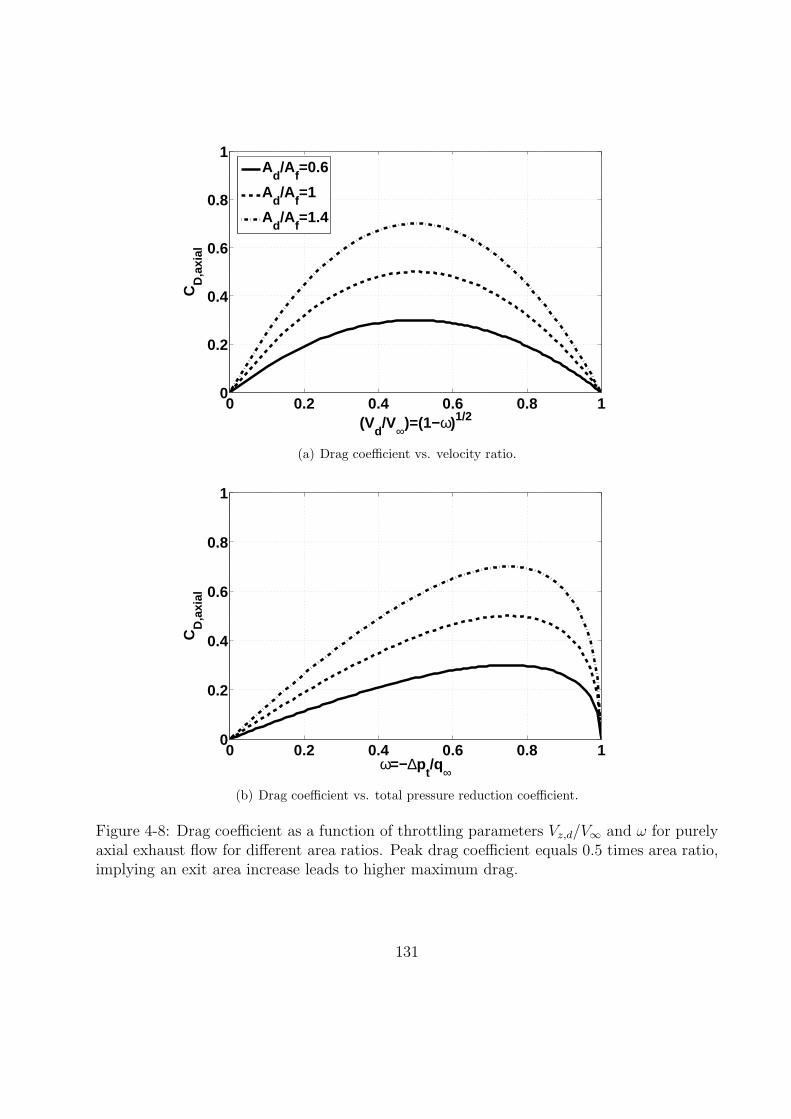
0 0.2 0.4 0.6 0.8 10
0.2
0.4
0.6
0.8
1
(Vd/V∞)=(1−ω)1/2
CD
,axi
al
Ad/A
f=0.6
Ad/A
f=1
Ad/A
f=1.4
(a) Drag coefficient vs. velocity ratio.
0 0.2 0.4 0.6 0.8 10
0.2
0.4
0.6
0.8
1
ω=−∆pt/q∞
CD
,axi
al
(b) Drag coefficient vs. total pressure reduction coefficient.
Figure 4-8: Drag coefficient as a function of throttling parameters Vz,d/V∞ and ω for purelyaxial exhaust flow for different area ratios. Peak drag coefficient equals 0.5 times area ratio,implying an exit area increase leads to higher maximum drag.
131

0 0.2 0.4 0.6 0.8 11
0.5
0
0.5
1
Vd/V∞
CD
Total
Nacelle
Actuator Disk
Dra
gT
hru
st
(a) Drag coefficient breakdown vs. velocity ratio.
0 0.2 0.4 0.6 0.8 1-1
-0.5
0
0.5
1
ω= ∆pt/q∞
CD
Dra
gT
hru
st
(b) Drag coefficient breakdown vs. total pressure reduction coefficient.
Figure 4-9: Drag coefficient breakdown for purely axial exhaust flow devices indicates thattotal drag is comprised of a drag force on the actuator disk and a thrust force on the nacelle.Shaded area indicates likely region of vortex shedding instability, as suggested by Figure 4-10.
that counteract the drag forces on the actuator disk, as discussed in chapter 2 of Greitzer
et al. [27]. This nacelle suction force may be identified by subtracting out the actuator disk
132

2.4
2.0
2.2
2.1
2.3
2.4
2.0
2.2
2.1
2.3
∞VV
d
1.00
0.75
0.50
0.25
0.10
0.01
Figure 4-10: Instantaneous unsteady contours of dimensionless entropy, Tt,∞s/V2∞, on 2D
CFD of deficit flow with varying velocity ratio at device scale Reynolds number. Nozzleheight is 2.16 meters. Computations indicate that vortex shedding instability develops atvelocity ratios . 0.25.
drag coefficient, CD,a.d., from the total drag, CD,axial,
CD,nacelle = CD,axial − CD,a.d. = CD,axial − ω. (4.24)
For the case of Ad/Af = 1, the three decomposed drag coefficients CD,nacelle, CD,a.d, and
CD,axial are presented in Figure 4-9. The figure demonstrates that the nacelle force is always
negative5, i.e., in the direction of thrust, with magnitude increasing rapidly with increased
loss coefficient or reduced exit velocity ratio.
In the limit of unity loss coefficient or zero velocity ratio, the model predicts zero total
drag, i.e., an equal balance between the actuator disk drag force and the nacelle thrust
5The reader is reminded of assumption 4 in Section 4.4.1, which states that the spilled flow remainsattached at the inlet. Violation of this requirement changes the validity of the model, due to flow separationand unsteadiness that is assumed deleterious to the low noise goals of the device.
133

force. This result is not physical, however, because zero velocity ratio corresponds to zero
throughflow, suggesting the onset of device-scale unsteady bluff body effects. This suggests
that the model is not valid below a critical velocity ratio, i.e. above a certain loss coefficient.
Unsteady computational fluid dynamics (CFD) solutions of a two dimensional, planar nozzle
flow with various velocity ratios presented in Figure 4-10 suggests that the critical velocity
ratio is about 0.25. The result is qualitatively and quantitatively similar to flow studies
on bluff body flows with and without supercritical base bleed [4, 78, 79, 96]. Contours of
entropy generation demonstrate that below this value bluff body effects generate large-scale
unsteady vortex shedding. This is a stability limit that constrains the validity of the model
(shown by the shaded area in Figure 4-9), and is assumed undesirable from a noise generation
point of view. The exit velocity ratio is also a mass flow capture fraction, which suggests
that excessively low throughflows should be avoided for acoustical reasons.
4.4.3 Swirling Flow Dynamics
The model for a purely axial flow device suggests that the theoretical maximum drag co-
efficient is limited to a value of 0.5 for Ad/Af = 1. Attention is now turned to swirling
flows, which are shown to theoretically outperform axial exhaust flows within the assumed
stable flow limits. This section provides a brief overview of swirling flow dynamics, while
the next section extends the drag model to swirling flows with a prescribed exit circulation
distribution.
Swirling flows have features that are significantly different from flows without swirl. All
real swirling flows are vortical structures6, that originate in the boundary layers of the
surfaces over which the working fluid moves. These surfaces shed vortex lines in a manner
consistent with the features of the flow. Behind a bluff body at high Reynolds number,
vortex lines originate as closed rings that lose their orientation relatively rapidly due to
random stretching from a highly turbulent wake. On a delta wing at high angle of attack,
6The mathematical concept of an irrotational swirling flow is called a free vortex, for which circumferentialvelocity is inversely proportional to radius. This flow exhibits a numerical singularity on the centerline whichis physically never realized due to the effect of viscosity.
134

flow separation occurs near the wing apex, resulting in the rolling up of two highly coherent
streamwise vortices that persist for many characteristic lengths downstream. In the case of
the swirl tube, the vortex lines are generated in the boundary layers of swirl vanes and the
nacelle end walls. Aft of the vanes these lines become aligned by the bulk fluid motion so as
to develop a strong streamwise component of vorticity at the duct exit.
Swirling flows have a more complex description than non-swirling flows because the equa-
tions of motion are non-linear and coupled in such a way to make simple analytical models
mathematically challenging. A key feature of highly swirling flows is strong radial pressure
gradients. In addition, axial and circumferential velocity components are usually highly
coupled, as energy conservation in the absence of lost work constrains the balance of kinetic
energy components (u2z/2, u
2θ/2) and flow work (p/ρ). The strong coupling means that vortex
cores become increasingly sensitive to far-field variations in pressure with increasing swirl.
Because of this sensitivity, excessive swirl leads to the vortex breakdown phenomenon, a
feature that is manifested as an abrupt change in flow properties. At high Reynolds number
this includes unsteadiness, turbulence, and rapid diffusion of primary vorticity. New insight
into the underlying physics of vortex breakdown is not a primary goal of this thesis. In-
stead, vortex breakdown is taken here to be a known phenomenon, studied extensively in
experiment, theory, and computation, that is important because it will set a limitation on
swirl tube performance. The effect of this limitation is a major unknown to be quantified in
Chapter 5.
Many of the dominant effects of swirling flow are inertial in nature [27]. Hence, the equa-
tions of inviscid, incompressible, axisymmetric flow are the starting point to examine some
of the critical aspects of swirling flow dynamics. Axisymmetry suggests that the natural
coordinate system be cylindrical, and defined by the radial, circumferential, and axial com-
ponents, (r, θ, d). By neglecting the viscous terms, the flow is described as pressure driven.
The continuity equation, and the axial, circumferential, and radial momentum equations are
respectively given as:
135

1
r
∂
∂r(rur) +
∂
∂z(uz) = 0 (4.25)
∂uz
∂t+ ur
∂uz
∂r+ uz
∂uz
∂z= −1
ρ
∂p
∂z(4.26)
∂
∂t(ruθ) + ur
∂
∂r(ruθ) + uz
∂
∂z(ruθ) = 0 (4.27)
∂ur
∂t+ ur
∂ur
∂r+ uz
∂ur
∂z= −1
ρ
∂p
∂r+
(ruθ)2
r3(4.28)
The circumferential momentum balance, Equation 4.27, states that the quantity (ruθ) is
constant following a fluid particle7. Changes in radius thus lead to changes in circumferential
velocity in a pressure driven flow. This concept is important in understanding the dynamics
of the flow with respect to effective area changes within a swirling streamtube.
The radial momentum balance, Equation 4.28, has two terms on the right hand side,
a radial pressure gradient that acts as a real force on a fluid particle, and an apparent
force term that comes from the centripetal acceleration of the fluid particle. This apparent
centrifugal force can be viewed as a radial gravitational field of strength 1/r3 acting on an
apparent density of strength (ruθ)2, where the density analogy is based on the observation
that (ruθ) following a fluid particle is constant [27]. In the absence of radial velocity the
flow is said to be cylindrical, or in simple radial equilibrium, satisfying:
∂p
∂r=ρu2
θ
r. (4.29)
The sign of the right hand side of Equation 4.29 is always positive, meaning that pressure
gradients are always radially outward in a swirling flow. For most natural and man made
unconfined swirling flows, the atmosphere or free stream acts as a mechanical sink that sets
7This is another statement of Kelvin’s theorem for an incompressible, inviscid flow with conservative bodyforces, which states DΓ/Dt = 0, where Γ =
∮
C~u · dℓ is defined as the circulation around a closed contour C.
For convenience C may be taken as a circle of radius r about the centerline.
136

a pressure boundary condition on the outer regions of the flow. Hence, swirling flows have
sub-atmospheric pressures. The pressure drag generated by the swirl tube is later shown to
be the dominant drag mechanism for the device.
Vortex Breakdown
(a) Spiral type.
(b) Bubble type.
Figure 4-11: Types of vortex breakdown, adopted from Leibovich [48].
Vortex breakdown, or vortex burst, is a phenomenon that occurs in swirling flows that
exceed a critical swirl threshold. It is characterized by a transition from a small, tightly-
bound vortex with high velocities to a larger, more-diffuse vortex with lower velocities. For
laminar flows three major types of vortex breakdown have been classified in the literature: 1)
137

Figure 4-12: Types of vortex breakdown from low to high swirl, adopted from Hall [28] basedon the photographs of Sarpkaya [74].
double helix, 2) spiral, and 3) axisymmetric, or bubble-type, though other minor variations
have also been noted [64]. Double helix-type breakdown occurs at the lowest swirl velocities,
spiral-type at higher swirl velocities, and bubble-type at the highest velocities. Figure 4-11 is
adopted from Leibovich [48], and shows flow visualizations of spiral- and bubble-type vortex
breakdown. These visualizations are generated in a vortex tube, i.e. a weakly diffusing
138

tube that creates an adverse pressure gradient in the streamwise direction. It is the adverse
pressure gradient that triggers the sensitivity in the vortex core mentioned earlier that leads
to the breakdown.
Figure 4-12, adopted from Hall [28], and based on the photographs of Sarpkaya [74] sug-
gests that the spiral breakdown evolves into the bubble breakdown with increasing swirl. As
the swirl tube is a high Reynolds number device, the bubble-type breakdown is expected to
characterize the flow field when critical swirl is exceeded. The bubble-type vortex break-
down is seen at the highest swirl levels, and increasing swirl moves the breakdown further
upstream [16]. For the swirl tube, a separation bubble near the duct exit may create an
effective blockage that reduces the throughflow and hence reduces the vane loadings and the
drag. It is also observed that the separation bubble is not closed at its rear, and is usually
characterized by increased unsteadiness and turbulence. As the size of the bubble is expected
to be at the size of the device for excessive swirl, this is viewed as potentially detrimental to
swirl tube acoustics.
Numerous physical explanations of the vortex breakdown phenomenon exist in the liter-
ature. Vortex breakdown theory has been grouped into four major classes by Delery [16]:
1) quasi-cylindrical approach and analogy to boundary layer separation, 2) solution of ax-
isymmetric Navier-Stokes equations, 3) concept of critical state, or wave theory, and 4)
hydrodynamic instabilities. As it is not a primary aim of this thesis to shed new light on
the fundamental nature of vortex breakdown, the reader is directed to important works and
reviews given by Delery [16], Hall [28], Leibovich [48] and Sarpkaya [74] for further details
on the phenomenon. A brief discussion of the concept of critical state is provided here to
elucidate the conceptual explanation that is adopted in this thesis.
The concept of critical state As reviewed by Hall [28], this concept is first proposed
by Squire [83] and is later modified by Benjamin [6] and others. Squire proposes that the
conditions for the possible existence of standing waves is a sufficient criterion for breakdown
because downstream disturbances can propagate upstream. Benjamin then suggests that
Squire’s critical state has an important but not exclusive role in explaining breakdown. His
139

own work explains breakdown as a “transition between two steady states of axisymmetric
swirling flow, being much the same in principal as the hydraulic jump in open channel
flow.” The transition is said to occur between supercritical and subcritical states, where the
former cannot support standing waves and the latter can. At a high level, their analyses [28]
involve combining the governing equations into a single partial differential equation in terms
of the circumferential component of a streamfunction, ψθ, the so-called Bragg-Hawthorne
Equation [5] for incompressible flow,
∂2ψθ
∂r2− 1
r
∂ψθ
∂r+∂2ψθ
∂z2=r2
ρ
dpt
dψθ−K
dK
dψθ, (4.30)
where ur = − (1/r) ∂ψθ/∂z, uz = (1/r)∂ψθ/∂r, K = ruθ, and pt is the stagnation pressure.
Stationary axisymmetric perturbations are then superimposed over a quasi-cylindrical flow,
Ψ (r, z), such that
ψθ (r, z) = Ψ (r, z) + ǫF (r, z)eγz . (4.31)
Eigensolutions of the equation are then examined to determine if at least one standing wave
is supported. If at least one eigenvalue, γ2, is negative, the criterion is met and the flow
is said to be subcritical, allowing disturbances to propagate upstream and trigger vortex
breakdown. Otherwise the flow is supercritical, indicating disturbances decay, and vortex
breakdown does not occur.
A quasi one-dimensional model of waves on vortex cores presented by Darmofal et al. [15]
for unconfined geometries suggests that the comparison of a convective speed and a wave
speed may provide a stability criterion that is consistent with the onset of vortex breakdown.
By assuming a Rankine vortex model of the swirling flow, a wave speed, c, is found to be
proportional to the level of circulation in the vortex core:
c2 =Γ2∞
8πA=u2
θ,max
2. (4.32)
Increasing swirl leads to increasing wave speed. This speed is compared to the assumed
140

uniform convective speed in the streamwise direction, uz. A criticality condition,
c
uz=uθ,max/
√2
uz> 1, (4.33)
is derived when the wave speed exceeds the uniform convective speed, such that disturbances
may propagate upstream. This leads to a critical swirl parameter, Sc, at the core radius:
Sc =uθ,max
uz>
√2 ≈ 1.41. (4.34)
The result provided by the quasi-one-dimensional model is a useful estimate when compared
to Benjamin’s value of 1.2. Again, a strong analogy exists between the concept of waves
on vortex cores and a compressible shock wave or a hydraulic jump. Stable flow is said to
be supercritical, because perturbations are convected downstream with the flow, whereas a
subcritical, high entropy solution develops beyond the critical swirl level.
Of greatest importance for the design of the swirl tube is the criterion for vortex break-
down. Delery’s summary [16] on this indicates that the existence of breakdown is not always
well posed, and the definition of a breakdown criterion can sometimes be ambiguous. How-
ever, the most important feature is the axial and swirl velocity distribution. The salient
feature of axisymmetric swirling flows near the breakdown threshold is a swirl parameter,
SD, of 1.2, defined by Delery as
SD =Γ0
V∞rc, (4.35)
where rc is the vortex core radius and Γ0 is the circulation around a circle of radius rc. This
swirl parameter is the inverse of a Rossby number. The critical value of SD of 1.2 is found
to be fairly consistent across the theoretical approaches that predict the vortex breakdown
criterion. The corresponding maximum flow angle is generally near 50.
In this thesis the swirl parameter, S, will be treated as the metric to judge the onset of
vortex breakdown:
141

S =uθ
uz
. (4.36)
S is simply the tangent of the swirl angle. This definition of swirl parameter allows it to be
plotted as a flowfield variable, and will be presented as such in the next chapter. It is worth
noting that the value of S that corresponds to 50 swirl angle is also 1.2, suggesting Sc, SD
and S are approximately consistent parameters. In the next subsection it is assumed that
the swirling flow stability limit occurs near a value of S = 1.2 at the Burger vortex core, or
critical radius. In Chapter 5 high-fidelity computations and experimental verification will
demonstrate that this assumption is quantitatively valid.
4.4.4 Drag Generating Swirling Exhaust Flow Devices
In this subsection the drag from a swirling exit flow is quantified by extending the control
volume analysis to such flows. A swirl parameter near S = 1.2 is assumed to indicate the
onset of vortex breakdown, setting the validity limit of the model. The radial coordinate, r,
is first non-dimensionalized to r∗ by the circular duct outer radius, rd, i.e.,
r∗ =r
rd. (4.37)
It is assumed that a total pressure change may occur at the actuator disk. For the case
of a ram pressure driven swirl tube, this would imply a total pressure loss, (and mass flow
throttling), whereas for a pumped swirl tube (defined in Section 4.3) the net total pressure
would rise due to the fan stage work. The dimensionless total pressure change is given as
ω (r∗) =pt,∞ − pt,d
12ρV 2
∞
= −∆pt (r∗)12ρV 2
∞
. (4.38)
Simple radial equilibrium (see Equation 4.29) is invoked next. Under this assumption, Equa-
tion 4.28 simplifies to a dimensionless form in terms of the pressure coefficient,
dp
dr=ρV 2
θ,d
r=⇒ dCp
dr∗=
2 (Vθ,d/V∞)2
r∗. (4.39)
142

The pressure coefficient at a radial location, r∗ is found by integrating the above equation.
Assuming that the circumferential velocity distribution is known, the pressure distribution
becomes
Cp (r∗) = −∫ 1
r∗
2 (Vθ,d/V∞)2
rdr, (4.40)
where r is the variable of integration. The atmospheric pressure boundary condition con-
strains Cp to equal zero at r∗ = 1. The total pressure at any radial location in the downstream
plane is defined as
pt,d = pd +1
2ρV 2
z,d +1
2ρV 2
θ,d = pt,∞ + ∆pt = p∞ +1
2ρV 2
∞ + ∆pt. (4.41)
Equation 4.41 can be manipulated to define the pressure coefficient at any radial location in
terms of ω, and the axial and radial velocities, such that
Cp (r∗) =pd − p∞
12ρV 2
∞
= 1 − ω (r∗) −(Vθ,d
V∞
)2
−(Vz,d
V∞
)2
. (4.42)
Finally, by combining equations 4.40 and 4.42, the axial velocity may be written as:
Vz,d (r∗)
V∞=
√
1 − ω (r∗) −(Vθ,d
V∞
)2
+
∫ 1
r∗
2 (Vθ,d/V∞)2
rdr. (4.43)
Hence in the steady, incompressible model of ducted swirling outflow, the total pressure
change and swirl velocity profiles, ∆pt (r) /q∞ and Vθ,d (r) /V∞, respectively, are sufficient to
describe the entire behavior of the device including:
• The total drag coefficient, as well as contributions from the axial momentum flux drag
and pressure drag terms.
• The total mass flow, and hence the spillage and the net nacelle forces.
• The exit velocity and pressure profiles, and the swirl parameter profile, and hence a
first indication of stability margin.
143

Results
The exit circulation distribution in the preliminary analytical modeling is specified as a
Burger vortex distribution [27]. This representation is typical of many naturally occurring
vortices [16]:
rVθ,d
rdV∞=
(Kc
rdV∞
)[
1 − exp
(
−1.26r2
r2crit
)]
(4.44)
The Burger vortex distribution is defined by two parameters, a circulation multiplier, K∗c =
Kc/rdV∞ and a critical radius, r∗crit = rcrit/rd. Toward r∗ = 0 the Burger vortex distribution
becomes a forced vortex (rvθ ∼ r2), while at large radii the distribution approaches a free
vortex (rvθ ∼ constant). The circulation distribution is smooth, with the transition from
forced to free vortex occurring at the critical radius. The factor 1.26 appears in the equation
to ensure that the maximum Vθ,d occurs at the critical radius.
The prescribed exit circulation distribution also defines the dimensionless circumferential
velocity profile, and hence the pressure coefficient given by Equation 4.42. Once the total
pressure change is prescribed as ω (r∗), Equations 4.40 and 4.42 may be combined to obtain
the axial velocity. These known quantities may be substituted into Equation 4.19 to yield
an explicit expression of the drag coefficient given by
144

CD =1
Af
∫
A
2
√
1 − ω (r∗) −(Vθ,d
V∞
)2
+
∫ 1
r∗
2 (Vθ,d/V∞)2
rdr
×
1 −
√
1 − ω (r∗) −(Vθ,d
V∞
)2
+
∫ 1
r∗
2 (Vθ,d/V∞)2
rdr
dA
︸ ︷︷ ︸
axial momentum flux drag coefficient
+1
Af
∫
A
∫ 1
r∗
2 (Vθ,d/V∞)2
rdrdA
︸ ︷︷ ︸
pressure drag coefficient
= CD,ax. mom. + CD,press..
(4.45)
Exit Flow Field It is useful to first examine the general features of the exit flow for
a particular swirl and total pressure change distribution. A simple ram pressure driven
swirl tube with total pressure change resulting from typical airfoil cascade profile losses of
ω = 0.08 is considered. For r∗crit = 0.5 and K∗c = 0.77 the total drag coefficient, CD, is found
to be 0.80. Figure 4-13 shows dimensionless profiles of axial velocity, circumferential velocity,
negative pressure coefficient and swirl parameter. Going from the outer radius toward the
core the swirling flow is characterized by decreasing pressure, in this case about 3.5 times the
freestream dynamic head on the duct centerline. Relative to freestream, the flow accelerates
in the core due to the low pressure, but decelerates at the outer radius, i.e., it is jet-like
(Vz/V∞ ∼ 2) on the core and wake-like (Vz/V∞ ∼ 0.6) at the outer radius. The prescribed
circumferential velocity approaches a forced vortex on the centerline. The swirl parameter,
S = Vθ,d/Vz,d, has a local maximum of 1.48, and is 1.08 at the critical radius. From the
vortex breakdown stability criteria given in Section 4.4.3, this flow is suggested to be near
the stability limit of S = 1.2 at the critical radius.
145

0 1 2 30
0.2
0.4
0.6
0.8
1
Vz/V∞
r/r d
rcrit*
(a) Axial velocity
0 0.5 1 1.50
0.2
0.4
0.6
0.8
1
Vθ/V∞
r/r d
rcrit*
(b) Circumferential velocity
0 1 2 3 40
0.2
0.4
0.6
0.8
1
-Cp
r/r d r
crit*
(c) Pressure defect
0 0.5 1 1.50
0.2
0.4
0.6
0.8
1
S=V
r/r d
rcrit*
/Vzθ
(d) Swirl parameter
Figure 4-13: Profiles of axial velocity, circumferential velocity, pressure coefficient, and swirlparameter for analytical swirl tube model with Burger vortex exit flow parameters of ω =−∆pt/q∞ = 0.08, r∗crit = 0.50, and K∗
c = 0.77, yielding drag coefficient of CD = 0.8.
If the exit total pressure is known everywhere, it is possible to characterize the tradeoffs
made between the static and dynamic pressure components along the profile through energy
conservation arguments. On the centerline the circumferential velocity approaches zero since
the flow resembles a forced vortex. Hence the total pressure is composed of the static pressure
146

and the axial component of dynamic pressure. This may be viewed as trading low pressure
for high axial velocity. On the outer radius, the static pressure equals the freestream, such
that along a streamline the circumferential dynamic pressure component is increased at the
expense of the axial dynamic pressure component. Hence circumferential velocity is traded
for axial velocity. One clear limit within the assumptions of the model then is that the
circumferential velocity may not be increased to the extent that the axial velocity stagnates
anywhere in the flow. For the Burger vortex circulation distribution of the current model the
maximum value of the swirl multiplier, K∗c , to avoid zero axial velocity on the outer radius
is given by
(K∗
c )max =
√1 + ω
1 − exp
[
−1.26
(r∗crit)2
] . (4.46)
Swirling flow dynamics suggests a tendency for stagnation and reverse flow to occur on the
centerline in bubble-type vortex breakdown; the limitation to flow stagnation on the outer
radius presented in Equation 4.46 at least qualitatively supports the notion that excessive
swirl may lead to an instability and hence unsteady flow.
The parameterized design space of 1) a ram pressure driven, or throttled swirl tube,
and 2) a fan driven, or pumped swirl tube are next explored to provide a more complete
picture of the effects of loss and swirl distribution on drag generation. In addition, design
recommendations are presented. The CD = 0.8 Burger vortex design point with radial
profiles presented Figure 4-13 is indicated in subsequent figures by a blue triangle.
Ram Pressure Driven Swirl Tube For the ram pressure driven swirl tube, total pressure
loss coefficient is assumed to have a constant value of ω = 0.08. Figure 4-14 presents
iso-contours of drag coefficient overlayed by iso-contours of swirl parameter at r = rcrit
in the design space defined by the dimensionless Burger vortex parameters K∗c and r∗crit.
The maximum swirl multiplier at each critical radius is given by Equation 4.46, and is
demarcated by the heavy dashed blue line. Solutions to the right of this line violate the
energy conservation constraint discussed earlier and thus do not exist.
147

0.2
0.2
0.2
0.4
0.4
0.4
0.6
0.6
0.6
0.8
0.8
1
1
1.2
1.4
0.4
0.4
0.4
0.8
0.8
0.8
1.2
1.2
1.2
1.6
2
Swirl K*c
r* cri
t
0 0.2 0.4 0.6 0.8 1 1.20.3
0.4
0.5
0.6
0.7
0.8
0.9
S CD
(K )c max*
Multiplier,
Figure 4-14: Contours of predicted total drag coefficient (CD, dashed red) and swirl parame-ter at r = rcrit (S, solid black) in (K∗
c , r∗crit) space for ram pressure driven swirl tube having
ω = 0.08. Triangle indicates point with CD = 0.8 and rcrit = 0.5, whose radial profiles arepresented in Figure 4-13. Heavy, dashed blue line indicates (K∗
c )max threshold.
The key design recommendation that emerges from the figure is that the highest drag
is associated with a highly swirling vortex with small core size. Drag coefficient contours
become closer together as K∗c increases, indicating that the rate of change of drag with
respect to maximum swirl level increases with swirl. Maximum CD values also increase with
decreasing r∗crit, with values above 1 at r∗crit . 0.5.
The highest levels of S at r = rcrit are found to be just above 1.2, suggesting that the
reverse flow limit derived from the axial/circumferential dynamic pressure balance arguments
is qualitatively in accord with the vortex breakdown criteria mentioned in the previous
subsection.
Figure 4-15 again presents iso-contours of drag coefficient overlayed by iso-contours of
capture stream tube to duct exit area, Acapt/Ad. The vertical axis defined by K∗c = 0 has a
148

0.2
0.2
0.2
0.4
0.4
0.4
0.6
0.6
0.6
0.8
0.8
1
1
1.2
1.40.7
5
0.8
0.8
0.85
0.85
0.850.
9
0.9
0.9
0.9
5
0.9
5
0.95
Swirl K *c
r* cri
t
0 0.2 0.4 0.6 0.8 1 1.20.3
0.4
0.5
0.6
0.7
0.8
0.9
Acapt
/Af
CD
(K )c max*
Multiplier,
Figure 4-15: Contours of predicted total drag coefficient (CD, dashed red) and capturestreamtube to actuator disk area ratio (Acapt/Af , solid black) in (K∗
c , r∗crit) space for ram
pressure driven swirl tube having ω = 0.08. Triangle indicates point with CD = 0.8 andrcrit = 0.5. Heavy, dashed blue line indicates (K∗
c )max threshold.
value of Acapt/Ad of 0.96, meaning that the total pressure loss of ω = 0.08 in the actuator disk
without swirl reduces mass flow by four percent, per Equation 4.22. The Acapt/Ad contours
indicate that mass flow decreases with increasing swirl, but the spilled mass flow from swirl
alone is rather small for drag coefficients below about 0.4. For high drag, high swirl cases a
throttling effect of ten to twenty percent mass flow reduction is seen relative to non-swirling
flow. Thus, another recommendation for a ram pressure driven swirl tube is that good inlet
design should incorporate a droop to avoid high incidence angle from this amount of spillage.
Figure 4-16 presents iso-contours of the two components of the total drag coefficient,
namely, the pressure drag, CD,press., and the axial momentum flux drag, CD,ax. mom., in the
(K∗c , r
∗crit) space. The figure indicates that the pressure drag dominates the overall drag
at high swirl. For example, in the CD = 0.8 design point indicated by the blue triangle,
149

0.2
0.2
0.2
0.4
0.4
0.4
0.8
0.8
0.8
1.2
1.2
1.6
2-0.4
-0.2
-0.2
-0.1
-0.1
-0.1
-0.0
5
-0.0
5
0
0
0
0.0
5
0.05
0.05
Swirl K*
c
r* cri
t
0 0.2 0.4 0.6 0.8 1 1.20.3
0.4
0.5
0.6
0.7
0.8
0.9
CD,press.
CD,ax. mom.
Multiplier,
-0.0
5
(K )c max*
Figure 4-16: Contours of predicted drag coefficients from pressure defect (CD,press., solidblack) and net axial momentum flux (CD,ax. mom., dashed red) in (K∗
c , r∗crit) space for ram
pressure driven swirl tube having ω = 0.08. Triangle indicates point with CD = 0.8 andrcrit = 0.5. Heavy, dashed blue line indicates (K∗
c )max threshold.
pressure drag is an order of magnitude larger than momentum flux drag, rendering the
latter essentially negligible8
At the fixed value of r∗crit = 0.5, the effect of loss and swirl parameter on drag coefficient
is presented in Figure 4-17. Iso-contours of CD are normal to the vertical direction along
the zero swirl line defined by S = 0, while at high swirl parameter levels these contours
are roughly normal to the horizontal direction. The key implication is that for high levels
of swirl, loss has a weak effect on the overall drag. Assuming a swirl parameter similarity
associated with a physical set of swirl vanes9, this figure suggests that loss goes from the
8The axial momentum flux drag actually has small negative values at high swirl, i.e., it theoreticallyproduces a thrust component, because the axial momentum excess on the centerline is greater than the axialmomentum defect at the outer radius.
9This is suggested in the pumped swirl tube computations of Section 5.5.1.
150

0.1
0.2
0.2
0.3
0.3
0.3
0.4
0.4
0.4
0.4
0.5
0.5
0.50.6
0.6
0.60.7
0.70.7
0.8
0.8
0.8
0.9
0.9
Swirl Parameter, S, at r=rcrit
Loss
Coe
ffici
ent,
ω
0 0.2 0.4 0.6 0.8 10
0.1
0.2
0.3
0.4
0.5
Figure 4-17: Contours of predicted total drag coefficient (CD) in (S, ω) space for ram pressuredriven swirl tube having r/rcrit = 0.5.
dominant drag mechanism at low swirl vane angles to a weak drag mechanism at high swirl
vane angles. This drives the design recommendation that for high drag coefficient, greater
emphasis should be placed on achieving the correct flow turning, with secondary emphasis
placed on the accuracy of loss modeling.
Pumped vs. Throttled Swirl Tube Comparison The total pressure change ∆pt/q∞,
is varied from positive (pumping) to negative (throttling) for fixed r∗crit = 0.5, in the range
of allowable swirl multiplier levels 0 to (Kc)max. Figure 4-18 presents iso-contours of CD and
S (at r = rcrit). In the pumped regime, negative values of CD correspond to net thrust.
Fixed values of S may be associated with a fixed set of swirl vanes. Hence, along a fixed
S iso-contour in the direction of pumping, CD decreases due to the fan stage work input.
However, for a given ∆pt/q∞, the difference in CD between a fan stage with purely axial exit
151

-5 -4.5
-4
-4
-3.5
-3.5
-3
-3
-2.5
-2.5
-2.5
-2
-2
-2
-1.5
-1.5
-1.5
-1
-1
-1
-1
-0. 5
-0.5
-0.5
-0.5
0
0
0
0
0.5
0.5
0.5
0.5
1
1
1
0.2
0.2
0.2
0.4
0.4
0.4
0.6
0.6
0.6
0.8
0.8
0.8
1
1
1
1.2
1.2
1.2
Swirl K*
c
∆p
t/q∞
0 0.5 1 1.5 2
0
1
2
3
4
CD
S
Multiplier,
pumped
throttled
Zero Force Line
(K )c max*
Figure 4-18: Contours of predicted total drag coefficient, CD (dashed red), and swirl pa-rameter, S (solid black), in (K∗
c ,∆pt/q∞) space for pumped or throttled swirl tube withr/rcrit = 0.5. Dashed blue line indicates (K∗
c )max threshold.
flow (K∗c = 0) and a swirling outflow case at fixed S increases in the direction of increased
pumping, suggesting that a pumped swirl tube generates greater effective drag through thrust
reduction, relative to a stand alone, ram pressure driven swirl tube with similar critical swirl
parameter (and hence, vane angle).
The three symbols in Figure 4-18 correspond to devices that illustrate this effect. A
ducted fan stage with pressure rise of ∆pt/q∞ = 3 having purely axial exhaust, shown by the
circle, may operate in parallel with a stand alone, ram pressure driven swirl tube with CD =
0.8, shown by the triangle. An alternate configuration is a pumped swirl tube having the
same total pressure rise and the same swirl vanes, and is marked by the square. The device
comparison is depicted in Figure 4-19. The difference in CD between the two configurations
suggests that a pumped swirl tube produces greater thrust reduction (CD = 3.5) relative to
152

+
Pumped Device – No Swirl
Throttled Swirl Tube
Fan Stage
Swirl Vanes
CD= - 4
CD=+0.8
Net CD= - 3.2 (thrust)
(a) Conventional fan engine plus stand alone, rampressure driven swirl tube.
Pumped Swirl Tube
Fan StageSwirl Vanes
Net CD=-0.5 (thrust)
CD=-4CD=+3.5
(b) Pumped swirl tube.
Figure 4-19: Comparison between conventional fan engine at approach idle plus stand alone,ram pressure driven swirl tube versus pumped swirl tube, for πfan = 1.06, M∞ = 0.17,Ad/Af = 1, suggests that pumping of swirl vanes generates greater effective drag in the formof thrust reduction.
a ram pressure driven swirl tube (CD = 0.8). Within the framework of the quiet approach
requirements analysis that assumes approach thrust is fixed by the go-around maneuver
requirement, thrust reduction is equivalent to drag generation. For a dimensionless total
pressure rise10 of ∆pt/q∞ = 3, the drag coefficient difference between purely axial exhaust
flow, CD = −4, and the maximum swirling flow drag coefficient, CD = −0.5, results in an
equivalent drag coefficient of 3.5, about 4 times larger than a stand alone, ram pressure
driven swirl tube with CD = 0.8. This amount of effective drag would be sufficient to change
the glideslope angle at constant approach velocity from 3 to 7, resulting in 7.4 dB potential
overall noise reduction if it were quiet.
The higher effective drag coefficient from pumping results from greater ingested mass
flow, leading to greater vane loadings. Figure 4-20 presents the same total drag coefficient
contours overlayed with iso-contours of captured steamtube area fraction, Acapt/Af . At
ω = ∆pt/q∞ = 3 the captured streamtube area is roughly twice that of a ram pressure
10The selected total pressure change across the fan stage of ∆pt/q∞ = 3 corresponds to a fan stage pressureratio of 1.06 at a flight Mach number of 0.17, typical of approach speeds for the SAX conceptual aircraftdesign described in Section 4.1.
153

-5
-4.5
-4
-4
-3.5
-3.5
-3
-3
-2.5
-2.5
-2.5
-2
-2
-2
-1.5
-1.5
-1.5
-1
-1
-1
-0.5
-0.5
-0.5
-0.5
0
0
0
0
0.5
0.5
0.5
0.5
1
1
1
0.60.8
0.81
11.21.2
1.2
1.41.4
1.4
1.6 1.6
1.6
1.6
1.8 1.8
1.8
1.8
22
22.2 2.2
Swirl K*
c
∆p
t/q∞
0 0.5 1 1.5 2
0
1
2
3
4
CD
Acapt/Af
pumped
throttled
Multiplier,
Zero Force Line
(K )c max*
Figure 4-20: Contours of predicted total drag coefficient, CD (dashed red), and capturestreamtube to actuator disk area ratio, Acapt/Af (solid black), in (K∗
c ,∆pt/q∞) space forpumped or throttled swirl tube with r/rcrit = 0.5. Dashed blue line indicates (K∗
c )max
threshold.
driven value ∆pt/q∞ = −ω = −0.08. Capture steamtube ratio at fixed S (at r = rcrit) is
a good general indicator of the ratio of flowfield velocities between two cases with different
total pressure changes. Higher velocities in the pumped case suggest a noise increase relative
to the ram pressure driven case, though a noise scaling law would have to be experimentally
determined. As the effective drag benefits of a pumped swirl tube come with a noise penalty,
it is recommended that these tradeoffs be quantified in future work.
The iso-contours of Acapt/Af also indicate that for high swirl a given ∆pt/q∞ has the ten
to twenty percent throttling effect relative to axial exhaust flow, as mentioned earlier. For
a fan driven system, this may affect operability of the turbomachinery. This suggests that
a wide operating range fan design for approach, or a variable area nozzle may be practical
technologies for propulsion system integration.
154

4.5 Chapter Summary
This chapter introduced the idea of a novel quiet drag device called a swirl tube. The
motivation provided here leads to the aerodynamic design and aerodynamic and acoustic
validation presented in the next chapter. The swirl tube idea is developed using mission
requirements analysis and parametric control volume modeling.
As the CMI Silent Aircraft Initiative has the goal of designing an aircraft that is func-
tionally silent outside a typical airport perimeter, a step reduction in noise is needed relative
to conventional aircraft. On approach, an aerodynamically and acoustically clean airframe
is required. In addition operational changes such as slower and steeper approach profiles
are required. This identifies the need for quiet drag, i.e., a departure from the strong corre-
lation between drag and noise of conventional devices such as flaps, slats, or landing gear.
Preliminary modeling indicates that:
1. Quiet drag requirements for the SAX conceptual aircraft to realize several decibels
noise reduction are comparable to the clean airframe drag. More generally, steepen-
ing a conventional glideslope from 3 to 6 requires quiet drag roughly equal to the
component of weight in the direction of the conventional glideslope.
2. Bluff body drag coefficients based on propulsion system fan area (CD about 1.0) are
capable of steepening a conventional glideslope from 3 to 4 at fixed approach speed,
potentially resulting in 2.5 dB noise reduction. Overall noise reduction of 5 or more
dB may be realizable through a combination of quiet drag coupled with quiet high-lift
devices that enable slow and steep flight.
A preliminary drag model has been developed for a ducted device with purely axial and
swirling exit flows, assuming steady, incompressible inflow and outflow. The model assumes
an axisymmetric actuator disk with area equal to the duct exit (Ad/Af = 1) imparts a
change in total pressure and swirl. For ram pressure driven devices with throttling, i.e., net
total pressure loss, the modeling results suggest:
155

1. A maximum drag coefficient of 0.5 is theoretically possible for a device with uniform
axial outflow at an exit to freestream velocity ratio, Vz,d/V∞, of 0.5, equivalent to a
non-dimensional total pressure change, −∆pt/q∞ = ω=0.75.
2. A swirl tube generates maximum drag coefficients greater than 0.8, a nearly two-fold
increase versus a purely axial outflow device.
3. The exit flow features of a typical swirl tube with high drag coefficient may include:
i) axial velocity excess (2V∞) on the centerline, ii) axial velocity defect (0.6V∞) at the
outer radius, and iii) high pressure defect at the centerline (3.5q∞).
4. The vortex breakdown instability is likely to set the limitation to maximum swirl tube
capability, near a swirl parameter of 1.2, or 50 exit flow angle. Hence a recommended
design would be close to but not in excess of this swirl parameter limit.
5. Loss of total pressure throttles the swirl tube mass flow. Loss increases drag at low
swirl, but has a weak effect on overall drag at high swirl. Design for high drag should
place greater emphasis on proper flow turning, with loss prediction being a secondary
consideration.
6. Stable swirling flow without additional losses reduces mass flow ten to twenty percent
at maximum drag relative to purely axial flow. A good swirl tube design should account
for this level of spillage by incorporating a droop in the inlet leading edge.
Scenarios with a net total pressure rise are also generated to simulate the interaction of
a swirl generator with an upstream fan stage. For a pumped swirl tube, the model suggests
that:
1. Swirl generation downstream of a fan stage generates high effective drag by reducing the
maximum thrust capability more than the drag produced by a separate, ram pressure
driven swirl tube. For a typical approach idle setting this may be several times the
ram pressure driven swirl tube drag.
156

2. The pumped swirl tube ingests greater mass flow than the ram pressure driven swirl
tube, suggesting that exit velocities will be higher and noise possibly scales to some
appropriate velocity ratio power law.
3. The throttling effect of swirl relative to axial exit flow suggests that a wide operating
range fan design or a variable area nozzle may be beneficial for propulsion system
integration.
157

158

Chapter 5
Swirl Tube: A Novel Turbomachinery
Concept for Mission 2
Chapter 4 introduces the concept of the swirl tube, a quiet drag device that generates a
ducted swirling outflow to enable slow and steep approach profiles for a functionally quiet
aircraft. A parametric study using a control volume analysis and a survey of swirling flow
dynamics suggests that high drag coefficients (CD & 0.8) may be achieved with stable,
highly swirling flows. This chapter presents the details of the aerodynamic design, and
computational and experimental validation of the swirl tube aerodynamics and acoustics.
A ram pressure driven swirl tube is found to be a viable quiet drag device at full-scale,
generating a scaled drag coefficient near 0.8 with noise signature well below the goals of a
functionally quiet aircraft. A successful design for high drag and low noise requires a stable,
swirling exit flow with maximum swirl angle near 50. The vortex breakdown phenomenon
is found to acoustically and aerodynamically limit swirl tube performance, by generating a
device-scale, unsteady separation bubble near the duct exit. Important aspects of the system
integration of a swirl tube with an airframe/propulsion system are explored at the end of
the chapter. Swirl generated downstream of a fan stage at approach idle setting, a so-called
pumped swirl tube, is found to produce large thrust reductions, relative to the drag of a
ram pressure driven device, suggesting a potential opportunity for additional quiet drag.
159
The increased mass flow and exit velocities that result from fan stage work require future
acoustic validation of this configuration.
5.1 Objectives
Two major hypotheses are tested in this research. The first hypothesis is that a swirl tube
can generate high drag coefficient (& 0.8) based on throughflow area, with exhaust flow
fields that contain no large-scale unsteadiness. The second hypothesis is that the flow fields
associated with the stable swirling exhaust flow are viable, quiet alternatives to high-drag
control surfaces (flaps, slats, spoilers) and landing gear, enabling their use on a quiet aircraft.
Testing these hypotheses requires meeting the following objectives:
1. Defining and quantifying the relationship between swirling flow, drag, and noise.
2. Quantifying the required swirling exit flow fields of the device.
3. Describing the limitations imposed on the device by the vortex breakdown phenom-
enon.
4. Characterizing swirl tube noise signature, identifying noise mechanisms and establish-
ing acoustic power scaling laws.
5. Identifying the system integration issues and challenges associated with the implemen-
tation of a swirl tube on a quiet aircraft.
5.2 Technical Approach
A technical roadmap of swirl tube research is presented in Figure 5-1. The objectives of
this research are met through aerodynamic design and aerodynamic and aeroacoustic ex-
perimental validation of swirl tubes with different swirl angle distributions. The final step
is to identify technical challenges associated with the implementation of swirl tubes into
160

Concept 2:
Swirl Tube
Aerodynamics
Design Space Exploration
Parametric Swirl
Waves on Vortex Cores
Nacelle LE Droop
Duct/Centerbody
Definition
Vane
Definition
Swirl Angle
Definition
3D CFD Predictions
(Single Passage Periodic)
Drag, Vortex Breakdown, Flowfield
Acoustics
System Integration
Aerodynamic Validation
(Wright Brothers Wind Tunnel)
Flow Viz, Drag, Steady Flowfield &
Unsteady Velocity Spectra
Aeroacoustic Validation (NASA Langley QFF)
Swirl Noise, Vortex Breakdown Noise
Scaling Law Extraction, Full Scale Spectra
Airframe
Propulsion System
System
Integration
ConceptsFan Stage Interaction
Thrust Reverser Comparison
Acoustic Analogy Based
Acoustic Models
Pre-test Predictions
Figure 5-1: Swirl tube technical roadmap.
the airframe/engine system. The technical approach is executed sequentially in remaining
sections, as described here.
Swirl tube aerodynamics are discussed in Section 5.3. Section 5.3.1 begins with a sweep of
the design space of a duct/centerbody geometry with parametrically defined internal swirl
distribution, using an inviscid, axisymmetric throughflow analysis tool, MTFLOW. MT-
FLOW output provides the first definition of the ducted swirl vane exit angles and exit flow
fields. Candidate vane exit angle distributions are selected from a family of swirl distribu-
tions for various drag coefficients. Sectional vane design methods in Section 5.3.2 then define
the three-dimensional blade geometry, for which single-passage periodic CFD computations
are performed using Fluent, as discussed in Section 5.3.3. The CFD computations include
the internal and external flow fields, and are intended to predict the drag coefficient and
161

give a description of the flow fields. The CFD computations also account for the viscous
nature of the vortex core, which MTFLOW does not. The Fluent computations identify
the critical conditions for the onset of the vortex breakdown instability. Finally, model-scale
aerodynamic tests at the MIT Wright Brothers Wind Tunnel (WBWT) conducted by the
author and Mobed [61] are described in Section 5.3.4. The goals of these tests are to 1)
experimentally validate the aerodynamic design and 2) identify potential noise source mech-
anisms that arise from unsteadiness in the flow field. The experimental validation is done
through drag measurements, flow field mapping and flow visualization. Unsteady velocity
signals measured from hot-wire anemometers indicate potential broadband acoustic source
regions.
Swirl tube acoustics are discussed in Section 5.4. To the author’s knowledge, the noise
signature of the flow field emanating from such a device has not previously been reported.
A major research challenge is to determine the swirl tube sound generation mechanisms and
scaling laws. A brief description of modeling efforts to estimate the noise from the swirling
flow are provided in Section 5.4.1. These noise models rely on CFD postprocessing, com-
bining jet noise concepts from Lighthill’s acoustic analogy [49, 50] with Tam et al.’s [88, 89]
adjoint Greens function solutions of the linearized Euler equations. Acoustic validation tests
at the NASA Langley Quiet Flow Facility are subsequently discussed in Section 5.4.2. Noise
spectra from swirl tubes with different swirl distributions are presented, with an emphasis
on comparison between stable swirling flow and vortex breakdown. Acoustic power scaling
laws are also deduced, as well as geometric scaling for aircraft application, demonstrating the
viability of the swirl tube for quiet drag on approach. In addition, the acoustic experiments
ultimately demonstrate that the aforementioned theoretical models fall short of capturing
the correct swirl tube noise sources or levels, indicating that more effort should be spent on
this type of noise modeling in future.
In Section 5.5 high-level system integration issues are presented. Swirl tube integration
into a propulsion system bypass or mixing duct is challenging because the downstream
resistance offered by swirl vanes affects the fan stage operating point. CFD computations
162
of swirl vanes downstream of an idealized fan stage (a so-called pumped swirl tube) are
presented in Section 5.5.1. These computations demonstrate that pumping increases the
mass flow through the swirl vanes, resulting in greater thrust reduction than a ram pressure
driven swirl tube. The computations also highlight the importance of a low approach idle
setting on overall quiet approach feasibility. The effect of swirl vanes downstream of a fan
stage on the fan operating point is also discussed. In Section 5.5.2 the effectiveness of a
quiet drag device is compared to a thrust reverser during the landing roll. Although not
mandated by aviation authorities, thrust reversers are shown to provide the most stopping
capability on a slippery runway. Hence, a recommendation is made to incorporate the swirl
tube device concept into the thrust reverser mechanism if a propulsion system-integrated
configuration is chosen.
5.3 Swirl Tube Aerodynamics
In Section 4.4 an analytical ducted drag generation model using a Burger vortex exit swirl
distribution and vortex breakdown limits from swirling flow dynamics supports the hypoth-
esis that a drag generating swirling exhaust flow device may generate high drag coefficients
(& 0.8), about twice the theoretical maximum of a drag generating axial exhaust flow throt-
tling device. In this section this hypothesis is confirmed through aerodynamic design and
computational and experimental validation of a swirl tube.
Conceptually, the design process begins in Section 5.3.1 with a sweep of the design space
using streamline curvature methods in an inviscid, axisymmetric flow solver. Important gas
path-design effects such as loss and blockage are also studied. A family of vane designs are
then generated in Section 5.3.2 and computationally modeled with CFD in Section 5.3.3.
The CFD includes viscous effects in the core and establishes the flow fields for the stable
cases. CFD also identifies the vortex breakdown threshold. In Section 5.3.4, wind tunnel
testing, including flow visualization, hot-wire anemometry, and drag measurement by force
balance is used to validate the swirl tube design process and hypothesized drag capability.
163

5.3.1 Two Dimensional Axisymmetric Computations
The swirl tube drag capability is modeled with an axisymmetric flow solver, MTFLOW [20],
within a design space of parametrically defined circulation distributions. Swirl vanes are
treated as actuator disks [34] of finite axial extent contained within a nacelle/centerbody
geometry. The output of MTFLOW contains the internal and external streamline trajectories
in the meridional (axial-radial) plane. Swirling flow streamline exit angles may be extracted
as a function of radius, providing the first step to three-dimensional vane design.
Computational Methods
MTFLOW is a collection of programs that allows for the viscous/inviscid analysis and design
of axisymmetric bodies, and is an extension of the Euler equations-based methods using
intrinsic streamline grids that are described by Drela [19]. It includes effects of swirl, heat
addition, loss and blockage. The flow solver is given the duct and centerbody geometry,
and allows for a discontinuity of blockage, entropy (loss), circulation (rvθ) plus a prescribed
rotational speed (to allow for shaft work transfer), and additional stagnation enthalpy due
to heat transfer or heat release, along the streamlines that pass through the swirl generating
stators (the actuator disk). As the swirl tube is adiabatic with no rotating parts, heat
transfer and work transfer are neglected. The maximum allowable swirl limit is found to
correspond to the development of waves on the vortex core, signifying the onset of the vortex
breakdown instability.
A duct and centerbody geometry are first designed assuming swirl vanes with a hub to
tip ratio, rH/rf , of 0.25. This is chosen to be consistent with preliminary fan designs for the
SAX BWB aircraft described in Section 4.1. The dimensionless duct geometry is shown in
Figure 5-2, with the actuator disk outer radius1, rf having the reference value of unity. The
actuator disk is defined in the region from z/rf = −0.23 to z/rf = 0.23. In this region, the
duct and center body form a constant cross-section annulus with outer radius 1 and hub to
tip ratio 0.25. The forward portion of the centerbody is designed as a 2.5 : 1 ellipse, and
1As the swirl tube idea is motivated by the available throughflow area of an engine duct, the subscript freferences the fan face.
164

2 1.5 1 0.5 0 0.5 1 1.5 20
0.5
1
1.5
z/rf
r/r f,
A/A
fNacelle Centerbody Area variation
min inlet area
exit plane
act. disk exit
act. disk inlet
Figure 5-2: Nacelle and centerbody geometry. Dotted red line shows cross-sectional areavariation normalized to annulus area at z/rf = 0 (actuator disk position).
the aft centerbody is designed to come to a sharp point at z/rf = 1.29, and is faired to the
constant radius hub section using a polynomial spline. The nacelle geometry is a drooped
airfoil with a chord length equal to ∼ 160% of the actuator disk outer diameter and maximum
thickness to chord ratio of ≈ 6%. The nacelle leading edge is a 3 : 1 ellipse with a 5 droop.
This droop is selected by visually examining the streamlines of a similar, undrooped elliptical
leading edge for a representative swirl generation case in order to minimize high angles of
attack on the nacelle leading edge due to spillage. The nacelle trailing edge is designed to
have an approximate thickness-to-chord of 0.5%. The exit area of the duct is chosen to be
equal to the actuator disk annular area. Therefore the exit diameter of the duct is smaller
than the actuator disk annulus outer diameter by the factor√
15/16.
The duct cross-sectional area variation, normalized to the actuator disk cross-sectional
area, is also shown as a dashed red line in Figure 5-2. One may infer from the CV analysis
of Section 4.4.1 that increasing the nozzle exit area increases the theoretical maximum drag
capability (Maximum CD also increases, because it is defined in terms of Af , not Ad). As
this effect is already well understood, a 1 : 1 area ratio between the actuator disk and the
duct exit is selected for simplicity. The minimum inlet area is shown to be ≈ 90% of the
165

annulus area. The area ratio between the minimum inlet area and the actuator disk is based
on an assumed cruise design Mach number at the actuator disk face of 0.66 and a Mach
number at the minimun inlet area of 0.85, to match a typical aircraft engine inlet geometry.
A gradual area change in the inlet diffuser section is selected to prevent flow separation.
The duct geometry is read by MTFLOW, with an actuator disk definition of the swirl
profile and uniform total pressure loss equaling 4% of the freestream dynamic pressure be-
tween the axial stations z/rf = −0.23 and z/rf = 0.23. In addition, a prescribed blockage
of 6% is chosen to model the vane thickness. The loss and blockage levels are selected to be
typical of turbomachinery cascades. The axial coordinate z/rf = 0 represents the stacking
location of the vane airfoil sections, and it is from this location that the flow domain is
dimensioned. The flow domain is defined two nacelle chord lengths upstream of z = 0 and
three nacelle chord lengths downstream of z = 0. The outermost radial bound of the domain
is two nacelle chords from the centerline (r = 0).
In exploring the design space, the swirl distribution in the annular actuator disk is based
on a circular Burger vortex-like circulation (rvθ) distribution. The Burger vortex is a realistic
representation of a stable vortex found in nature [27], because it has a smooth and continuous
rvθ distribution, approaches a forced vortex (rvθ ∝ r2) in the core, and approaches a free
vortex (rvθ ∝ constant) away from the core2. The two dimensionless parameters that define
the Burger vortex are maximum swirl level, K∗c = Kc/rfV∞, and critical radius, r∗crit =
rcrit/rf . As the quantity rVθ is convected along streamlines in steady, axisymmetric, inviscid
swirling flow3, and the duct flow evolves from annular to circular as the centerbody ends, it
is advantageous to prescribe the changes in circulation across the annular actuator disk as a
function of streamline coordinate, ψ, in MTFLOW [20]. The Burger vortex-like circulation
(rvθ) distribution is thus mapped from radial to stream function coordinates under the
assumption of a circular Burger vortex with uniform axial velocity,
ψ
ψcrit=
(r
rcrit
)2
. (5.1)
2See Equation 4.44.3See Section 4.4.3.
166

(a) Supercritical (converged) case: Pressure coefficient distribution for K∗
c = 0.77, r∗crit = 0.7,CD = 0.80.
(b) Subcritical (unconverged) case: Pressure coefficient distribution showing standing wave-like be-havior along centerline for K∗
c = 1.10, r∗crit = 0.7. Standing wave is indicative of vortex breakdown.
Figure 5-3: MTFlow pressure coefficient (Cp) distributions for supercritical and subcritical(vortex breakdown) swirling flow.
In other words, the steamfunction coordinate ψ is an indication of the mass flux contained
within the streamtube of radius r, assuming uniform axial velocity. The Burger vortex-like
circulation distribution is thus defined as
rVθ
rfV∞= K∗
c
[
1 − exp
(
−1.26ψ
ψcrit
)]
. (5.2)
Convergence and Stability
MTFLOW generates an initial streamline grid through the domain, based on the geometry
and the prescribed actuator disk parameters. The code then iteratively adjusts the stream-
lines, along which the value of rvθ is prescribed, until all governing equations are satisfied
167

within a prescribed convergence criterion. Converged solutions show an increasing pressure
defect with increasing swirl. Figure 5-3(a) shows the pressure coefficient distribution of a
converged solution at the parameter values of K∗c = 0.77 and r∗crit = 0.7, with predicted drag
coefficient of 0.80.
For a fixed r∗crit = 0.7, solutions become unstable at some critical value of maximum
swirl level. This observation is consistent with the vortex breakdown instability shown to
occur at a critical value of swirl parameter in many classic swirling flows [6, 15, 16, 30].
Standing waves on the vortex core are found to develop during the iterations, as depicted
in Figure 5-3(b) for the parameters K∗c = 1.10 and r∗crit = 0.7. The concept of critical state
for vortex breakdown was presented in Section 4.4.3 as the condition where standing waves
are supported. In MTFLOW, solutions do not converge at the onset of these cases; hence,
non-convergence in MTFLOW is associated with the vortex breakdown instability.
Results
Figure 5-4 presents MTFLOW generated iso-contours of total drag coefficient (CD) and duct
exit swirl parameter (S) at ψ = ψcrit, plotted in the design space of the non-dimensional
maximum circulation and vortex core radius, K∗c and r∗crit =
√ψ∗
crit, respectively. These
iso-contours are shown for converged cases only, i.e., the blank area to the right of the heavy
dashed blue line corresponds to unconverged solutions that are associated with the vortex
breakdown instability. At the highest swirl levels, MTFLOW finds converged cases with
CD > 1.
Comparing Figure 5-4 to the analytically derived results of Figure 4-14 suggests that the
preliminary analytical models capture the CD and S iso-contour trends. For low levels of drag
(CD ∼ 0.2) and swirl parameter (S ∼ 0.4), the values of constant CD and S roughly match,
while at higher values they do not. This is because as swirl level increases, the uniform axial
velocity assumption employed in the MTFLOW swirl distribution expression (Equation 5.2)
becomes increasingly weaker. The low pressure, non-swirling region on the centerline creates
a high axial velocity (trading low static pressure for high axial dynamic pressure), while
168

0.2
0.2
0.2
0.4
0.4
0.4
0.6
0.6
0.6
0.8
0.8
1
1
1.2
1.2
1.4
0.4
0.4
0.4
0.8
0.8
0.8
1.2
1.2
1.6
2
Swirl K*c
r* cri
t
0 0.2 0.4 0.6 0.8 1 1.20.3
0.4
0.5
0.6
0.7
0.8
0.9
Multiplier,
SC
D
Figure 5-4: Contours of MTFLOW computed total drag coefficient (CD, dashed red) andduct exit swirl parameter at ψ = ψcrit (S, solid black) in (K∗
c , r∗crit) space for ram pressure
driven swirl tube having ω = 0.08. Triangular and circular symbols represent converged(K∗
c = 0.77, r∗crit = 0.7) and unconverged (K∗c = 1.10, r∗crit = 0.7) cases shown in Figure 5-3.
Dashed blue line demarcates boundary between converged and unconverged solutions.
the highly swirling flow on the outermost radius has nearly atmospheric pressure and low
axial velocity (trading low axial dynamic pressure for high swirling dynamic pressure). This
causes streamlines to become bunched toward the centerline, effectively reducing the core
radius. The radial shift of the core relative to the prescribed value of r∗crit is an artifact of the
uniform axial velocity assumption, and is the likely reason that unconverged solutions appear
at values of S well below 1.2 for lower values of r∗crit. In addition, the minimum achievable
vortex core radius in real swirling flows is limited by viscous effects that are neglected in
MTFLOW. On the other hand, for high values of r∗crit MTFLOW admits solutions with
values of S well above 1.2, beyond the regime of observed vortex breakdown onset [16]. As
the goal of the entire endeavor is to design a family of swirl tubes of increasing flow angle
169

that spans stable and vortex breakdown flowfields, these mitigating factors suggest that an
intermediate critical radius whose solutions span the assumed vortex breakdown indicator
of S = 1.2 represents a sound design choice. A parametrically designed family of vanes
of intermediate radius, r∗crit = 0.7 (ψ∗crit=0.49), is thus presented in the next subsection for
various drag coefficients. The moderate critical radius of 0.7 is recommended as a compromise
between excessive turning at the outer edge near the nozzle shear layer for large r∗crit, and
excessive core vorticity for a small r∗crit which may compare poorly to a real swirling flow
that has large viscous dissipation in the core.
Effect of Prescribed Actuator Disk Loss and Blockage
The effects of prescribed actuator disk loss and blockage are studied on a constant vane exit
angle basis in order to understand their implications on the accuracy of the drag predictions.
Low levels of loss and blockage consistent with turbomachinery (. 12%) are considered,
because the device concept consists of a ducted cascade of swirl vanes. The key findings are:
• Loss is found to have a second-order effect (. 10%) on the drag levels.
• Local blockage in the actuator disk increases the exit swirl parameter and hence drives
the flow toward vortex breakdown.
For the purposes of a swirl vane design methodology, changes in effective loss and blockage
provide a means to explain small discrepancies between measured and predicted drag as
discussed in Section 5.3.4. During a first design iteration it is recommended to place greater
emphasis on achieving sufficient flow turning. If a second design iteration is required the
values of loss and blockage may be adjusted to provide greater accuracy to the predicted
levels. A summary of the loss and blockage computational experiments is provided below.
Loss. Loss is increased by a factor of three, from the baseline case of 4% to 12% of
freestream dynamic head. It is found that increasing the loss the can theoretically in-
crease or decrease the drag, depending on whether the drag is dominated by a defect in
170

axial momentum or pressure, as given by Equation 4.19. This observation is consistent
with the analytical result presented in Figure 4-17 in Section 4.4.4. For the baseline case of
CD = 0.40, a three-fold increase in the loss results in an increase in drag to CD = 0.44. For
the baseline case of CD = 1.10 the opposite is true – a three-fold increase in loss results in a
drag reduction to CD = 1.06. The physical mechanism present can be explained as follows:
increasing the loss reduces the mass flow and also the flux of axial momentum through the
swirl tube. Since turning angle is held fixed between cases, this results in a reduced swirl
velocity magnitude and reduced pressure defect (from Equation 4.39). At low turning an-
gles (. 35), the reduction in axial momentum flux drag from an increase in actuator disk
loss is greater than the reduction in pressure drag, resulting in greater overall drag. At the
highest turning angle near the critical vortex breakdown swirl parameter (& 50), the axial
momentum flux drag is the weaker term compared to the pressure drag and hence a small
increase in loss can result in lower overall drag.
Blockage. Blockage is increased by two-fold from 6% to 12%, holding swirl vane angle
fixed for a low drag case. The resulting baseline drag coefficient of CD = 0.40 is found to
increase to CD = 0.47. Blockage creates an area constriction in the vane passages. Since
the duct exit area remains unchanged, negligible change in mass flow is found. Hence the
duct exit axial velocity is also relatively unchanged. The axial and circumferential velocity
through the actuator disk must thus increase to satisfy mass conservation. The increase in
circumferential velocity at fixed radii implies an increase in rvθ, which is a quantity that is
convected along the streamlines (from Kelvin’s theorem, Section 4.4.3). Finally, this results
in higher values of rvθ at the duct exit, compared to the relatively unchanged axial velocity at
the same station. The observed increase in drag coefficient also corresponds to an increase in
swirl parameter. The design implication of this for high swirl vane angles is that an increase
in effective blockage may trigger vortex breakdown. Therefore, vane angle setting should
compensate for blockage effects, with higher blockage values requiring lower blade angles in
order to achieve a given exit flow field.
171

CD,MTFLOW αmax
0.40 34
0.60 41
0.80 47
1.00 53
1.10 57
1.31 64
Table 5.1: Maximum vane turning angle (rounded to nearest degree) associated with dragcoefficient computed by MTFLOW.
5.3.2 3D Vane Design Methodology
The output of the design space exploration in the previous subsection provides flow angles
at the actuator disk exit station for various swirl distributions. Vane exit angles are thus
obtained for MTFLOW computed drag coefficients of 0.40, 0.60, 0.80, 1.00, 1.10, and 1.31,
the latter two being very close to the vortex breakdown condition based on MTFLOW
convergence behavior. Vane inlet angles are assumed to be 0. All geometries are based
on the selected critical radius value of 0.7, i.e., ψ∗crit = (0.7)2 = 0.49, from Equation 5.2.
Table 5.1 shows the maximum vane turning angles associated with these designs.
As swirl tube vane passages are accelerating the flow, the 3D vane design methodology
is conceptually similar to the design of turbine stators, and consists of designing airfoil
sections at constant spanwise stations between the leading and trailing edge radii of each of
the MTFLOW streamlines. An example of a typical airfoil section is shown in Figure 5-5.
Cubic Bezier splines, defined by four control points, define the pressure side of each spanwise
section, using a fixed set of parameters4. Circles are located along the pressure side points
to create an envelope that defines the suction side. The circle size is decreased to tailor
4Two control points set the pressure side leading and trailing edge. Since inlet and exit angles are known,tangents can be extended from each point. Each tangent has one additional control point along it, definedby the fraction of the distance from the leading (or trailing) edge point to the intersection point of the twotangents. These fractional values are fixed at 60% and 80% from the leading and trailing edges, respectively,for all vane sections.
172

−0.2 0 0.2 0.4 0.6 0.8
0
0.1
0.2
0.3
0.4
0.5
0.6
0.7
0.8
0.9
Axial Coordinate
Pitc
hwis
e C
oord
inat
e
Figure 5-5: Example of sectional vane design for inlet (upstream) angle, θu, of 0, exit(downstream) angle, θd, of 60 and solidity, σ, of 3. The pressure side (red), is defined usinga Bezier spline. Suction side (green) is defined by the area distribution of circles. Leading(black) and trailing (magenta) edges are 3:1 half-ellipses.
the area of the passage to have a favorable pressure gradient5, minimizing the risk of flow
separation. The leading and trailing edges of the blade are designed as 3 : 1 half-ellipses.
Figure 5-6 shows the result of stacking up the radial sections into a 3D vane.
A linear solidity function defines the blade chord length from hub to tip, on the basis
of twenty vanes. A count of twenty vanes is chosen to satisfy the solidity requirement and
ensure that the axial extent of the vanes fits within the constant cross-section annular region
5A smooth area distribution for all vane geometries was found by trial and error to be:
A
Au= 1 + η (1 + cosπtn)
(cos θu
cos θd− 1
)
(5.3)
where Au is the inlet (upstream) area, η = 0.35, n = 1.2, and t is the Bezier spline parameter for the pressureside, ranging from 0 at the leading edge to 1 at the trailing edge. t varies approximately linearly with theaxial coordinate of the pressure side.
173
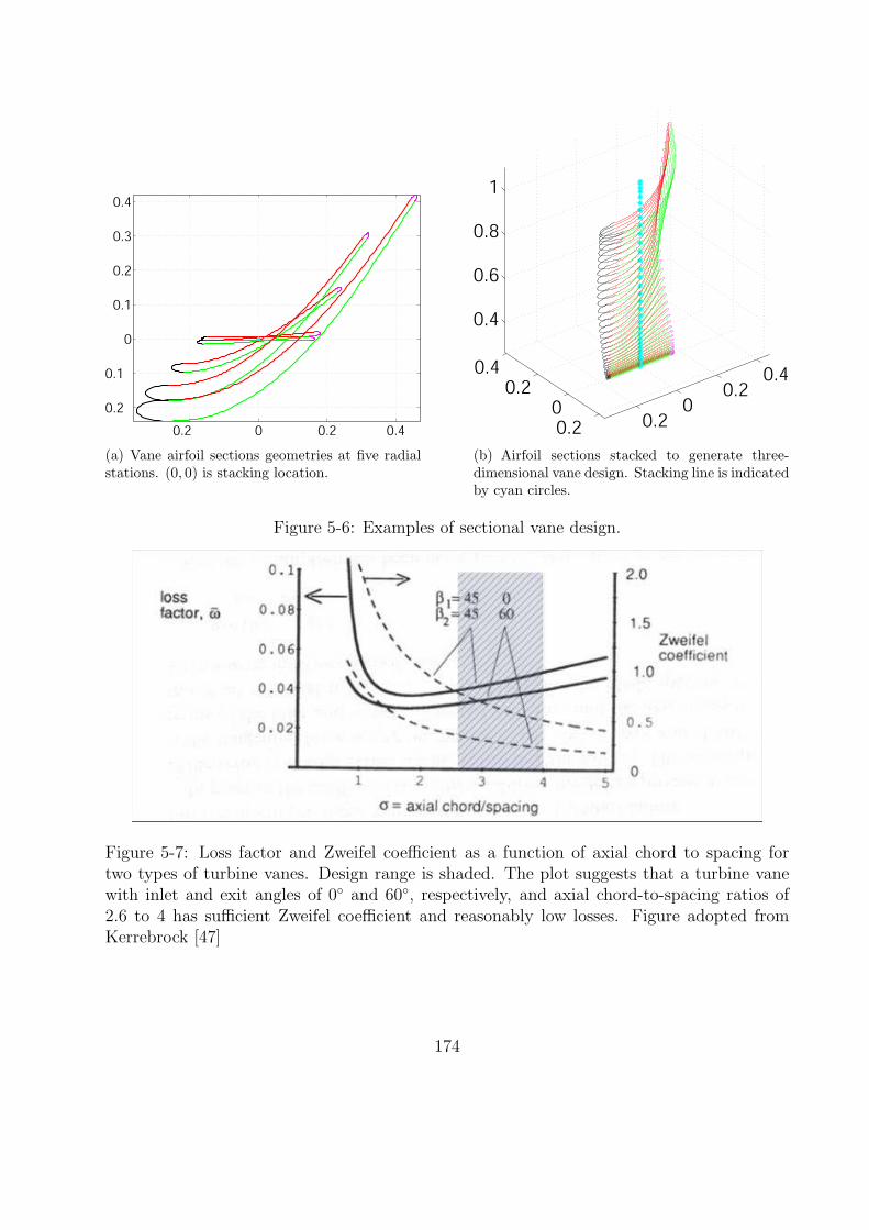
0.2 0 0.2 0.4
0.2
0.1
0
0.1
0.2
0.3
0.4
(a) Vane airfoil sections geometries at five radialstations. (0, 0) is stacking location.
0.20
0.20.4
0.20
0.20.4
0.4
0.6
0.8
1
(b) Airfoil sections stacked to generate three-dimensional vane design. Stacking line is indicatedby cyan circles.
Figure 5-6: Examples of sectional vane design.
Figure 5-7: Loss factor and Zweifel coefficient as a function of axial chord to spacing fortwo types of turbine vanes. Design range is shaded. The plot suggests that a turbine vanewith inlet and exit angles of 0 and 60, respectively, and axial chord-to-spacing ratios of2.6 to 4 has sufficient Zweifel coefficient and reasonably low losses. Figure adopted fromKerrebrock [47]
174

of the duct described in Section 5.3.1. Solidity is defined as vane chord divided by spacing.
The solidity varies monotonically from 3 at the tip to 4 at the hub. The axial chord divided
by spacing varies from 2.6 at the tip to 4 at the hub. As depicted in Figure 5-7 adopted
from Kerrebrock [47], the solidity range suggests low profile losses, as well as low Zweifel
coefficient [98], i.e., blade loading. Low loadings ensure that the flow is properly turned
within the vane passage, with minimal deviation.
5.3.3 Three Dimensional CFD Computations
The swirl vane and nacelle/centerbody design completes the geometric definition of the
various swirl tubes. A preliminary indication of swirl tube drag coefficient is obtained from
MTFLOW assuming an inviscid, axisymmetric flowfield. As the vortex core region of the
swirling exhaust flow is affected by viscosity and is turbulent at high Reynolds numbers,
higher fidelity modeling is warranted to improve the predicted drag and flowfield ahead of
experiments. Engine-scale, single passage periodic, steady CFD computations are performed
using Fluent for the subset of swirl tubes in Table 5.1 with maximum local vane angles of
34, 47, 53, 57, and 64. The objectives of the CFD computations are to: 1) predict which
swirl vane angles result in vortex breakdown, 2) compare the 3D single passage periodic flow
fields to MTFLOW to validate the preliminary scan of the design space, 3) define the exit
flow fields with the effect of viscosity included, and 4) provide a higher fidelity drag estimate
for the stable cases.
Computational Method
The standard Reynolds Averaged Navier-Stokes (RANS) k−ǫ turbulence model is employed
in Fluent to capture the effect of turbulent mixing in regions of high shear. Each case is
run to between 10,000 and 20,000 iterations to ensure low (. 10−4), decaying residuals in
converged cases (stable flow), and numerically stable (unchanging) residuals in unconverged
cases (vortex breakdown). It is found that the cases with 34, 47, and 53 swirl vane angle
converge, while the cases with 57 and 64 swirl vane angle do not converge due to formation
175

Z
Y X
(a) Swirl tube (gray and gold) and outer domainpressure far-field boundaries (blue) shown.
Z
Y X
(b) Zoomed-in view of Figure 5-8(a) showing one-half of swirl tube wall geometry (nacelle in gray,vanes in gold).
Figure 5-8: Typical CFD domain replicated to show ten periodic passages.
of a centerline separation bubble indicative of vortex breakdown.
A full-scale geometry is selected to simulate high Reynolds numbers seen in practical use.
The outer diameter of the swirl vanes is set to 2.16 meters, comparable to the preliminary fan
diameter of the CMI SAX conceptual aircraft powerplant or a large commercial fan engine
on a conventional civil airliner.
Computational domains are single passage periodic based on twenty vanes (wedges of
18), and include the internal and external flow field, to capture the forces on the vanes and
the nacelle forces that arise from spillage. The first computational domain generated for the
case with 34 vane angle extends roughly 4.5 nacelle lengths upstream and downstream of
the vane stacking station (z = 0). The outer domain is located roughly 2 nacelle lengths
from the centerline. All computational grids have approximately 1.2 million cells. As flow
profile non-uniformities and centerline gradients increase with swirl angle, it is found that a
substantial increase in axial grid resolution is required to ensure convergence. In order to keep
the total number of grid cells approximately constant, the downstream domains of all cases
except the 34 swirl vane angle are reduced to be the same as the MTFLOW computational
domain, namely, 2 nacelle chords lengths upstream and 3 nacelle chords downstream of the
176

vane stacking station. The outer domain is also located 2 nacelle chords from the centerline.
Figure 5-8(a) shows the smaller domain bounds used for all swirl tube cases except 34,
and Figure 5-8(b) presents an enlarged view of one-half of a typical swirl tube to give the
reader an indication of the relative dimensions of the nacelle/centerbody and swirl vanes.
The axial direction is indicated by the z-axis. The half-geometries are generated by nine
periodic replications of the CFD domain, as indicated by the solid black lines.
The upstream, downstream, and outer radial boundary conditions are set to pressure
far-field in Fluent, with Mach number equal to 0.17 and the freestream direction set to
positive z. Ambient density is based on a representative approach altitude. Rotationally
periodic boundaries are 18 apart and are bounded by the three pressure far-field boundaries.
Although the domain extends to the centerline, a specific centerline boundary condition is
not required. The surfaces of the swirl vane, the nacelle and the centerbody are modeled as
adiabatic walls.
Flowfield Comparison Between Stable (47 Swirl Angle) and Vortex Breakdown
(57 Swirl Angle) Cases
Figures 5-9 through 5-11 present flow field comparisons between the 47 and 57 swirl vane
angle cases. The figures compare Mach number (M), swirl parameter (S), and pressure coeffi-
cient (Cp), respectively. The Mach number comparison demonstrates that vortex breakdown
occurs between the swirl vane angles of 47 and 57. Numerically, the breakdown mani-
fests itself as a separation bubble on the centerline very close to the duct exits. As these
are steady single passage periodic computations based on 20 vanes, one would only expect
the three-dimensionality of the unsteady breakdown flow field to be captured qualitatively.
The CFD computations give an idea of the size and extent of the separation bubble. The
swirl parameter comparison of Figure 5-10 suggests that the critical swirl parameter for
vortex breakdown is close to 1.2, consistent with other studies on the vortex breakdown
phenomenon [6, 16] and results shown in Figure 5-4 for rcrit/rf = 0.7. The pressure coeffi-
cient distribution, Cp, suggests that the maximum pressure defect is roughly 3.5 times the
177

freestream dynamic head. In the exit flow field the pressure defect gradually decreases in
the streamwise direction for the stable case of 47 swirl vanes, while a more abrupt reduc-
tion of Cp defect occurs at the separation bubble – analogous to the abrupt change across
a hydraulic jump or a one-dimensional compressible shock wave undergoing transition from
super- to sub-critical state.
0.38
0.30
0.20
0.10
0.00
M
(a) 47 swirl vanes.
(b) 57 swirl vanes.
Figure 5-9: Mach number on periodic boundary of CFD cases.
Figure 5-12 shows the pressure coefficient distribution over the swirl tube surfaces for the
47 swirl angle case. No adverse pressure gradient occurs along the vanes in the streamwise
direction, suggesting the vane design methodology is sound. It is also apparent that the
stagnation point occurs at the drooped nacelle leading edge, validating the selection of droop
angle and inlet design. A downstream plane located at 0.5 nozzle exit diameters downstream
of the trailing edge shows the radial extent of the pressure defect in the swirling flow.
Overall, the flow field and surface pressure comparisons indicate that:
• the flow regime transitions from stable, steady swirling flow to unsteady vortex break-
down between swirl vane angles of 47 and 57.
• the vortex breakdown separation bubble occurs near the duct exit, suggesting adverse
178

2.5
2.0
1.5
1.0
0.5
0.0
-0.5
S
(a) 47 swirl vanes.
(b) 57 swirl vanes.
Figure 5-10: Swirl parameter on periodic boundary of CFD cases.
1.5
0.0
-1.5
-3.0
-4.5
-6.0
Cp
(a) 47 swirl vanes.
(b) 57 swirl vanes.
Figure 5-11: Pressure coefficient on periodic boundary of CFD cases.
acoustic implications from increased unsteadiness in the vicinity of solid surfaces and
edges.
• the computations confirm that the swirl parameter of about 1.2 is a good indicator of
vortex breakdown for this type of flow.
179

1.5
1.2
0.9
0.6
0.3
0.0
-0.3
-0.6
-0.9
-1.2
-1.5
-1.8
-2.1
-2.4
-2.7
-3.0
-3.3
-3.6
-3.9
-4.2
-4.5
Cp
Figure 5-12: Pressure coefficient, Cp, on surfaces of swirl tube with 47 vane angle show lowpressure at vane hub and aft centerbody. Radial extent of pressure defect is seen in plane0.5 duct diameters downstream of exit. Maximum pressure defect in downstream plane isCp ≈ −3.5.
• the maximum pressure defect of 3.5 dynamic heads for the 47 and 57 swirl vane angle
cases suggests that the maximum achievable drag occurs near these swirl angles, and
that the 47 design will be most favorable in terms of drag and acoustics.
Comparison to MTFLOW
CFD computed radial profiles of Mach number, pressure coefficient, swirl angle, and (rvθ)
are compared in Figure 5-13 at the duct exit for the swirl tube with 47 vanes. The inviscid,
axisymmetric flow approximation employed in the MTFLOW cases agrees well with CFD for
each of the radial profiles, validating the preliminary design methodology using MTFLOW.
180

Expected discrepancies occur near the outer radius and the centerline, because CFD cap-
tures the viscous effects at the endwall boundary layer and the vortex core. One erroneous
numerical feature that turns out to have little effect on the overall flow field is the finite swirl
angle on the centerline in the CFD solution. As this occurs at r∗ . 0.1, pressure forces in
0.1 0.2 0.3 0.4 0.50
0.2
0.4
0.6
0.8
1
Mach No.
r*
MTFLOW
CFD
(a) Mach number radial profile.
6 4 2 0 20
0.2
0.4
0.6
0.8
1
Cp
r*
(b) Pressure coefficient radial profile.
0 20 40 600
0.2
0.4
0.6
0.8
1
Flow Angle, α
r*
(c) Swirl angle radial profile.
0 0.2 0.4 0.6 0.80
0.2
0.4
0.6
0.8
1
rVθ/(r
fanV∞
)
r*
(d) Circulation radial profile.
Figure 5-13: MTFlow vs CFD comparisons for case with 47 swirl vanes.
181

MTFLOW CFDαmax CD CD CD,press. CD,visc. Vortex Breakdown Convergence34 0.40 0.39 0.32 0.07 No Yes47 0.80 0.75 0.68 0.07 No Yes53 1.00 0.84 0.77 0.07 No Yes57 1.10 0.89 0.82 0.07 Yes No64 1.31 0.94 0.38 0.06 Yes No
Table 5.2: MTFLOW vs. CFD drag coefficient comparison. Total drag coefficient is givenby CD. Pressure and viscous drag coefficients are given as CD,press. and CD,visc., respectively.
this region only act over . 1% of the duct area, and have little effect on the CFD-predicted
drag.
Table 5.2 compares the computed drag coefficient from MTFLOW to the CFD. For stable
cases, there is some drag coefficient discrepancy between the two methods, because the
MTFLOW computations do not include viscous drag components, whereas the CFD does.
In general, the MTFLOW drag estimates are higher than the CFD. This is not unreasonable,
as examination of the exit profile of Cp in Fig 5-13 shows a greater pressure defect in the
MTFLOW cases on the annulus between 5 and 30 percent exhaust duct radius. The CFD
computations do show greater pressure defect at the core below 5 percent exhaust duct
radius, but this acts over a relatively small area (35 times smaller than the aforementioned
annulus). As vortex breakdown is inherently unsteady, the steady CFD drag predictions are
not quantitatively meaningful for the two highest swirl vane angle cases.
In summary, MTFLOW is a useful preliminary design tool that captures the pressure-
driven regions of the swirling flow field accurately, and provides streamline exit angles for
three-dimensional vane design. CFD provides the best preliminary estimate of vortex break-
down onset, and suggests qualitatively the extent of the vortex breakdown separation bubble.
CFD also gives the most accurate pre-test prediction of drag levels and exit flow fields, ac-
counting for viscous and turbulence effects. This completes the aerodynamic design of the
various swirl tubes and leads to wind tunnel validation testing presented in the next section.
182

5.3.4 Model Scale Wind Tunnel Testing
Scale-model aerodynamic tests are next performed in the MIT Wright Brothers Wind Tunnel
(WBWT). The primary test objective is to validate the aerodynamic design. This requires 1)
flow visualization to identify swirl angles at which vortex breakdown occurs, 2) measurement
of exit flow field velocity profiles using hot-wire anemometry, and 3) measurement of drag
using a load cell and comparison to CFD computed values. Measured drag may also be
inferred by integration of steady velocity profiles obtained through hot-wire anemometry
(for the stable flow cases).
A second test objective is to determine potential noise sources, to guide the subse-
quent acoustic tests. This is accomplished by taking unsteady hot-wire measurements in
the swirling flow downstream of the duct exit and identifying regions of unsteadiness that
may correspond to potential quadrupole noise sources, i.e., ones that arise from turbulence
in open flows [18, 49, 50].
The full test matrix consisting of smoke and oil flow visualization, drag measurements,
and steady and unsteady hot-wire measurements in the flow field downstream of the nozzle
exit is shown in Table 5.3. A selected subset of the results is shown in this thesis. Details of
the entire test, including a facility description, are provided in Mobed [61].
Test Article
A picture of the swirl tube mounted in the WBWT is shown in Figure 5-14. The outer
diameter of the model swirl vanes is 7.036 inches (0.179 meters), i.e., at 12:1 scale relative
to the full-scale CFD diameter of 2.16 meters. Nacelle and centerbody parts are fabricated
from aluminum, and plastic swirl vane sub-assemblies have been fabricated using stereo
lithography (SLA). The SLA parts are designed as a one-piece annular cascade of 20 vanes
with integral inner (hub) and outer (nacelle) walls. The outer walls have forward and aft
flanges to smoothly mate in a modular fashion with the forward and aft nacelle parts. This
vaned disk enables easy interchanging of different swirl tube geometries. The swirl tube
is mounted on an airfoil shaped pylon designed to transmit loads to a force and moment
183

(a) Forward looking aft view of MIT Swirl Tube. (b) Swirl tube in WBWT.
Figure 5-14: WBWT wind tunnel experimental set-up.
balance located underneath the wind tunnel floor. Boundary layers are tripped by applying
tape with forward facing serrations near the leading edges of the vanes, inner and outer
nacelle, and pylon, to ensure fully turbulent flow, as expected in full-scale device operation.
Details of the mechanical design are found in Mobed [61].
M = 0.06 M = 0.06 M = 0.03 − 0.17 M = 0.03 M = 0.11Steady UnsteadyVelocity Velocity Drag Smoke Surface Oil
Configuration (Hot-wire) (Hot-wire) (Load Cell) Visualization VisualizationPylon Only ×
Empty Nacelle ×0 Blisk ×34 Blisk × × × × ×41 Blisk × ×47 Blisk × × × × ×53 Blisk ×57 Blisk × × × × ×64 Blisk × × × × ×
Table 5.3: WBWT test matrix.
184

(a) Smoke visualization. (b) Identical image as (a) with centerlines super-imposed to indicate core axial smoke streak.
Figure 5-15: Flow visualization close to the centerline axis identifies a coherent vortex corewithin a steady swirling flow for the stable flow cases (34, 41, and 47 swirl vanes) and alarge unsteady core for the cases with vortex breakdown (57 and 64 swirl vanes).
Flow Visualization
Instantaneous flow visualization images acquired at 30 frames per second for swirl tube vane
angles of 34, 41, 47, 57, and 64 are presented in Figs. 5-15 and 5-16. Smoke is injected
185

(a) Smoke visualization. (b) Identical image as (a) with wavelength esti-mate for pre-breakdown cases indicative of flowangle and graphic representation of outer swirlingflow for vortex breakdown cases.
Figure 5-16: Flow visualization at the outer radius identifies a tightly spiraling, steadyswirling flow for stable cases (34, 41, and 47 swirl vanes) and indirectly infers an outercoherent swirling flow for vortex breakdown cases (57 and 64 swirl vanes).
via a hand-held heated wand that vaporizes liquid glycol upstream of the swirl tube. As
flow is essentially incompressible (M∞ ≤ 0.17) and weakly Reynolds number dependent at
186

all test points, dynamic similarity allows selection of a low freestream velocity (∼ 20 m/s) to
minimize turbulent diffusion of the smoke streakline. By moving the smoke injection location
radially, the dynamics of the swirling flow both near the vortex core and in the outer annular
areas are revealed. The two figures show instantaneous smoke streaklines in the core region
and at outer radial locations, respectively.
In the core region the smoke streaklines for the 34, 41, and 47 swirl vane cases clearly
show a straight line of smoke on the axis of symmetry, surrounded by a tightly coiling helical
smoke trail around the core. From this one can infer that the core in these stable cases is
a coherent, tightly swirling flow structure. The fact that the line of smoke appears straight
at the centerline stems from the fact that the Burger vortex-like rvθ distribution selected to
generate the vane exit angles has zero turning at the hub, such that the low momentum fluid
that is in the boundary layers of the centerbody and vanes near the hub exits the swirl vanes
axially. The vanes are designed to turn the flow significantly just a short distance away from
the hub, such that the helical smoke streakline wraps itself tightly around this core. The flow
visualization for cases with 57 and 64 swirl vanes clearly shows a device-scale, cloud-like
smoke pattern just downstream of the exit, indicative of bubble-type vortex breakdown6, in
good agreement with CFD predictions presented earlier in Figure 5-9.
Smoke visualization at the outer radial locations in Figure 5-16 reveals the outer flow
dynamics. For example, the wavelength of the helical coil formed by the streaklines in the
stable cases becomes shorter as the swirl angle increases, as expected. The instantaneous
picture of the 57 case shows what appears to be coherent outer swirling flow around the
burst vortex. Although it is difficult to visualize in the instantaneous images presented in
the thesis, it becomes apparent when viewing the image series at 30 frames per second. The
graphic in the right column of the 57 swirl vane case qualitatively describes the streakline
shape of the coherent outer swirling flow.
The flow visualizations confirm that the steady, single passage periodic domain CFD
captures the onset of vortex breakdown. In the next section experimentally measured velocity
profiles from the swirling exhaust flow are compared to CFD to quantitatively assess the
6see Section 4.4.3
187

+1.5 R
+1.0 R
+0.5 R
0.0 R
-0.5 R
-1.0 R
-1.5 R
0.5 D 1.0 D 2.0 D 4.0 D
Swirl
Tube Z
R
100 Records (Unsteady)Single Record (steady)
+1.5 R
+1.0 R
+0.5 R
0.0 R
-0.5 R
-1.0 R
-1.5 R
0.5 D 1.0 D 2.0 D 4.0 D
Swirl
Tube Z
R
100 Records (Unsteady)Single Record (steady)
Figure 5-17: Hot-wire traverse locations for steady and unsteady measurements. All mea-surements are taken in the vertical plane that passes through the swirl tube centerline.
accuracy of the predictions.
Hot-wire Anemometry
Steady and unsteady velocity measurements are made in the vertical plane passing through
the swirl tube centerline using hot-wire probes at locations depicted in Figure 5-17. Un-
steady axial and circumferential velocity signals are obtained by orienting the probe’s wire
perpendicular to these respective directions, under the assumption of zero radial velocity
component, i.e., simple radial equilibrium. Each time record is sampled at 40 kHz with a
total of 16,384 points, resulting in a sampling time of 25µs and an overall record length of
0.4096 seconds. For steady measurements, the average value of single records are computed
along radial traverses at axial stations of 0.5, 1.0, 2.0, and 4.0 nozzle diameters downstream
of the nozzle exit. For unsteady measurements, the power spectra of 100 consecutive records
are computed at 0.0, 0.5, 1.0 and 1.5 nozzle radii at the same axial stations. All hot-wire
measurements are made at a freestream Mach number of 0.06. Further details of the hot-wire
experimental procedure are provided in Mobed [61].
Steady Velocity Measurements. Figs. 5-18 to 5-20 compare CFD predicted and ex-
perimentally measured values of dimensionless axial and circumferential velocity, along with
computed swirl angle, for the 34, 47, and 57 swirl vane cases, respectively, at axial sta-
188

0 0.5 1 1.5 21.5
1
0.5
0
0.5
1
1.5
Vz/V∞
r/r d
CFD
Experiment
(a) Axial Velocity, z/D=0.5
1 0 11.5
1
0.5
0
0.5
1
1.5
Vθ/V∞
r/r d
(b) Circumferential Velocity,z/D=0.5
50 0 501.5
1
0.5
0
0.5
1
1.5
Swirl Angle
r/r d
(c) Swirl Angle, z/D=0.5
0 0.5 1 1.5 21.5
1
0.5
0
0.5
1
1.5
Vz/V∞
r/r d
(d) Axial Velocity, z/D=2.0
1 0 11.5
1
0.5
0
0.5
1
1.5
Vθ/V∞
r/r d
(e) Circumferential Velocity,z/D=2.0
50 0 501.5
1
0.5
0
0.5
1
1.5
Swirl Angle
r/r d
(f) Swirl Angle, z/D=2.0
Figure 5-18: Axial velocity, circumferential velocity, and computed swirl parameter (S) vs.radial location for case with 34 swirl vanes. Top row, z/D = 0.5, bottom row z/D = 1.0.
tions z/D = 0.5 (top row) and 1.0 (bottom row). The experimental measurements for the
stable cases (34 and 47) show good agreement with CFD. The size and shape of the viscous
core are well captured. The computed swirl angle measurements are favorable, though slight
overturning of several degrees appears to be a feature of the stable cases at z/D = 0.5.
Maximum stable duct exit swirl angles of about 50 are achieved in the 47 swirl vane case.
In the 47 swirl vane angle case, the location of the vortex center appears to be below the
geometric centerline at z/D = 0.5, and slightly above the geometric centerline at z/D = 1.0.
When compared to the 34 and 57 swirl vane cases this asymmetry is striking. It is not
clear whether this is due to a slight error in the radial positioning of the hot-wire probe or
a physically displaced vortex center. A possible conjecture is that the flow is near the onset
189

0 0.5 1 1.5 21.5
1
0.5
0
0.5
1
1.5
Vz/V∞
r/r d
uc
tCFD
Experiment
(a) Axial Velocity, z/D=0.5
1 0 11.5
1
0.5
0
0.5
1
1.5
Vθ/V∞
r/r d
uc
t
(b) Circumferential Velocity,z/D=0.5
50 0 501.5
1
0.5
0
0.5
1
1.5
Swirl Angle
r/r d
uct
(c) Swirl Angle, z/D=0.5
0 0.5 1 1.5 21.5
1
0.5
0
0.5
1
1.5
Vz/V∞
r/r d
uct
(d) Axial Velocity, z/D=2.0
1 0 11.5
1
0.5
0
0.5
1
1.5
Vθ/V∞
r/r d
uct
(e) Circumferential Velocity,z/D=2.0
50 0 501.5
1
0.5
0
0.5
1
1.5
Swirl Angle
r/r d
uc
t(f) Swirl Angle, z/D=2.0
Figure 5-19: Axial velocity, circumferential velocity, and computed swirl parameter (S) vs.radial location for case with 47 swirl vanes. Top row, z/D = 0.5, bottom row z/D = 1.0.
of the vortex breakdown instability, where a standing wave, or perhaps a minor precession
of the vortex core offsets its center of rotation from the axis of symmetry, as depicted
by the laminar spiral vortex breakdown images in Figure 4-11. This conjecture warrants
further investigation because the acoustic spectrum of the 47 swirl vane case presented in
Section 5.4.2 has a shape that may be indicative of the flow regime cross-over between stable,
swirling flow and vortex breakdown.
The 57 swirl vane angle case suggests that there is coherent swirling flow at the outer
radial locations, at indicated by the qualitatively well captured axial and circumferential
velocity profiles between 0.75 and 1.0 radii at both axial stations. At lower radii, there is
disagreement, indicative of the size and presence of a vortex breakdown separation bubble,
190

0 0.5 1 1.5 21.5
1
0.5
0
0.5
1
1.5
Vz/V∞
r/r d
uc
tCFD
Experiment
(a) Axial Velocity, z/D=0.5
1 0 11.5
1
0.5
0
0.5
1
1.5
Vθ/V∞
r/r d
uc
t
(b) Circumferential Velocity,z/D=0.5
50 0 501.5
1
0.5
0
0.5
1
1.5
Swirl Angle
r/r d
uct
(c) Swirl Angle, z/D=0.5
0 0.5 1 1.5 21.5
1
0.5
0
0.5
1
1.5
Vz/V∞
r/r d
uct
(d) Axial Velocity, z/D=2.0
1 0 11.5
1
0.5
0
0.5
1
1.5
Vθ/V∞
r/r d
uct
(e) Circumferential Velocity,z/D=2.0
50 0 501.5
1
0.5
0
0.5
1
1.5
Swirl Angle
r/r d
uc
t(f) Swirl Angle, z/D=2.0
Figure 5-20: Axial velocity, circumferential velocity, and computed swirl parameter (S) vs.radial location for case with 57 swirl vanes. Top row, z/D = 0.5, bottom row z/D = 1.0.
and consistent with flow visualization in Figs. 5-15 and 5-16. This disagreement stems from
the fact that the flow in the separation bubble is highly unsteady and does not satisfy simple
radial equilibrium, making the hot-wire probe unable to identify the mean flow direction
below r/rd ∼ 0.75.
Taken in toto, the steady hot-wire measurements quantitatively validate that CFD com-
putations accurately describe the stable flowfield in the near exhaust (z/D . 1.0), and
qualitatively confirm the nature of the bubble-type vortex breakdown.
Power Spectra of Unsteady Velocity Components. Figure 5-21 presents power spec-
tra of the unsteady axial and tangential velocity components one diameter downstream of
191

0 5 10 15 20
10−4
10−2
100
102
Frequency (kHz)
Pyy
, (m
2 /s3 )
47°
57°
(a) Pyy of unsteady axial velocity, Vz
0 5 10 15 20
10−4
10−2
100
102
Frequency (kHz)
Pyy
, (m
2 /s3 )
(b) Pyy of unsteady circumferential velocity, Vθ
Figure 5-21: Power spectra of unsteady axial and tangential velocity in core region, r∗ = 0,at axial location one diameter downstream of nozzle exit, z/D = 1.0. Data is presented atconstant bandwidth of 2.44 Hz.
the duct, z/D = 1.0, in the core region of the flow, i.e., the swirl tube centerline, r∗ = 0.
Similar power spectra in the shear layer region, i.e., r∗ = 1, are presented in Figure 5-22.
192

0 5 10 15 20
10−4
10−2
100
102
Frequency (kHz)
Pyy
, (m
2 /s3 )
47°
57°
(a) Axial velocity, V 2z
0 5 10 15 20
10−4
10−2
100
102
Frequency (kHz)
Pyy
, (m
2 /s3 )
(b) Circumferential velocity, V 2
θ
Figure 5-22: Power spectra of unsteady axial and tangential velocity in shear layer region,r∗ = 1, at axial location one diameter downstream of nozzle exit, z/D = 1.0.
As the downstream location is far from the surfaces of the swirl tube, the power spectra
are suggested to provide guidance about the presence of possible quadrupole noise sources,
193

i.e., ones arising from turbulence in open flow. The wind tunnel is set to a freestream Mach
number, M∞, of 0.06 during the data acquisitions7. Power spectra of both velocity compo-
nents are included because there is no a priori knowledge of whether the turbulence has any
preferred direction. The spectra are presented in linear narrowband format at a constant
bandwidth of 2.44 Hz.
At frequencies below 10 kHz, velocity power spectra are generally broadband in nature.
At 10kHz a spike appears in all cases and at both radial locations and axial locations. This
spike is likely to be spurious electrical noise, as it does not match any expected Strouhal
numbers (based on device length scales) or measurement apparatus natural frequencies. At
frequencies above 10 kHz, many of the spectra appear to have additional sharp tones. These
are also likely to be spurious, as acoustic spectra presented in Section 5.4.2 at similar Strouhal
number suggest primarily broadband acoustic sources at high frequencies.
The spectra between the stable flow and vortex breakdown cases compare differently in
the core (Figure 5-21) and shear layer (Figure 5-22) regions. On the core the stable swirling
flow case (47 swirl vanes) has levels of spectral energy that are generally at least one order
of magnitude greater than corresponding spectra of the vortex breakdown case (57 swirl
vanes). The tangential velocity power spectrum of the 47 swirl vane case suggests greater
acoustic energy than the corresponding 57 swirl vane case spectrum at all frequencies. The
axial velocity power spectrum of the 47 swirl vane case suggests lower acoustic energy at
low frequency, but greater acoustic energy at high frequency. Spectral comparisons at axial
stations z/D = 0.5 and z/D = 2.0 are in accord with these observations. This suggest the
possible presence of a more pronounced quadrupole source on the core in the case of the
stable swirling flow versus the vortex breakdown flow, especially at the highest frequencies.
In the shear layer the level of spectral energy is similar between the two cases, though
slightly stronger for the case with 57 swirl vane angle. Although the velocity profile varies
between cases, the shear layer power spectra do not vary greatly, suggesting that the shear
7As a reference to the reader, a Strouhal number of unity based on this velocity (near room temperature)and swirl tube exit diameter is close to 100 Hz. In Section 5.4.2 most acoustic spectra are presented forM∞ = 0.17, implying a unity Strouhal number close to 300 Hz.
194

layer noise may be similar to other known shear layer flows. Overall, the spectra suggest
that the core region may have a unique noise signature in the case of the stable, swirling
flow, and that the acoustic differences in shear layer region may be less pronounced between
the two flows.
It should be noted that overall noise levels are difficult to judge based on the spectra.
As will be shown in Section 5.4.2, the vortex breakdown flow noise is much louder (∼ 15
dB) than the stable flow noise, but concentrated at the duct exit (hence not quadrupole
in nature), where unsteady data is not taken. Two hypotheses (that will be confirmed in
Section 5.4.2) may be drawn from the unsteady spectral comparisons:
1. The noise spectra are largely broadband in nature.
2. The stable, 47 swirl vane angle case is likely to have increased quadrupole noise sources
in the core region, relative to the 57 swirl vane angle case with vortex breakdown.
Drag Measurements
Drag is experimentally measured in WBWT for comparison to converged CFD predictions
for stable exit flows, and to quantify the swirl tube drag capabilities for stable and vortex
breakdown exit flows. The experimentally measured drag coefficient represents an average
value of drag coefficients taken at various freestream Mach numbers between M = 0.06 and
M = 0.17. The three key results from the measurements are:
1. Experimentally measured drag coefficient is found to be higher than CFD predicted
drag8 by up to 0.08, but can be plausibly explained by small differences in flow turning
observed in the steady velocity profiles taken with hot-wire anemometry.
2. A maximum stable flow model-scale drag coefficient of 0.83 is measured for the 47
swirl vane angle case, demonstrating high drag coefficient (& 0.8) for steady swirling
outflows. Full-scale drag coefficient estimate based on a Reynolds number correction
8Only CFD predictions from converged, stable flow cases are compared to measured cases without vortexbreakdown, i.e., 34 and 47 swirl vanes.
195

Experiment (model-scale) CFD (corrected to model-scale)Case CD CD,visc. CD,press. CD,int. CD CD,visc. CD,press.
Pylon Only 0.42Empty Nacelle 0.08
0 0.14 0.14 0.0034 0.52 0.14 0.38 0.48 0.44 0.12 0.3247 0.83 0.14 0.69 0.81 0.80 0.12 0.6853 0.85 0.14 0.71 V.B. 0.89 0.12 0.7757 0.82 0.14 0.68 V.B. 0.94 0.12 0.8264 0.76 0.14 0.62 V.B. 0.98 0.10 0.88
Table 5.4: Table of measured and CFD computed drag coefficients for model-scale geometry.All CD values are referenced to the axially projected swirl vane annulus area. CFD valuesof viscous drag coefficient, CD,visc., are corrected to model-scale using Reynolds numbercorrection of Equation 5.4. Pylon drag is shown for reference only, and is subtracted out ofall other cases.
suggest drag coefficients of 0.78 and 0.79 for vane outer diameters of 2.16 and 1.20
meters9, respectively.
3. Maximum drag coefficient occurs near the flow regime change from stable swirling flow
to vortex breakdown.
Table 5.4 compares CFD predicted drag coefficients with those obtained experimentally
at WBWT. All numbers correspond to model-scale geometry. Direct swirl tube drag mea-
surement is made with the force and moment balance. Pylon alone drag is first measured
and then subtracted from the drag of each of the swirl tube test articles, including an empty
nacelle and the case with 20 straight vanes (0 turning). The swirl tube experimental drag
from the force balance is given by CD. The measured drag coefficient of the case with 20
straight vanes is estimated to equal the experimental viscous drag coefficient, CD,visc., for all
of the swirl tube cases, as it has similar surface area. The difference between CD and CD,visc.
is thus assumed to equal the experimental pressure drag, CD,press.
92.16 meters corresponds to the CFD computations based on the fan diameter of an early variant ofthe SAX powerplant. 1.20 meters corresponds to the final SAX powerplant fan diameter, and is used forfull-scale noise spectral extrapolation in Section 5.4.2
196

For the stable 34 and 47 swirl vane cases, total drag coefficient is also independently
estimated by integration10 of the hot-wire axial and circumferential velocity profiles at z/D =
1.0, assuming the flow satisfies simple radial equilibrium (vr = 0). It is given in the table by
CD,int.. Pressure defect integration is a two-step procedure involving a pressure coefficient
profile computation followed by pressure drag coefficient computations, as given by the
equations of Section 4.4.1. The drag estimate from measured velocity profile integration of
the stable cases is consistent to within 0.04 of the drag coefficient values measured on the
force and moment balance. The CFD drag coefficient is calculated by force integration over
the swirl tube vane, nacelle and centerbody surfaces (CD). The total drag is made up of a
viscous and pressure component, CD,visc. and CD,press., respectively, obtained from shear and
normal force integration over these surfaces. As CFD is performed at full-scale (12:1 relative
to the model), a Reynolds number correction is applied to the viscous drag component based
upon turbulent flat plate skin friction coefficient, [77], which is inversely proportional to the
1/5th power,
Cf ∝ Re1/5 (5.4)
The correction suggests that the CFD viscous drag coefficient increases from 0.07 to 0.12 at
model-scale.
Figure 5-23 presents measured CD as a function of swirl vane angle, and compares CFD
predicted values for converged, stable flow cases. The figure and Table 5.4 indicate that a
higher drag coefficient is measured in the experiment relative to the CFD, for the exper-
imental cases that do not undergo vortex breakdown (≤ 47 swirl vane angle). The drag
coefficient measurement error is conservatively estimated at 0.03, based upon the maximum
difference between individual drag coefficient measurements at different Mach numbers and
the average drag coefficient, for all cases. The discrepancy in drag coefficient is suggested to
occur from the slight overturning measured in the steady hot-wire traverses. Overturning is
10The station z/D = 1.0 is chosen for the integration because it displays good symmetry above and belowthe centerline (r/rduct = 0). Absolute values of Vz/V∞ and Vθ/V∞ can then be averaged between theupper and lower profiles. In addition, because the hot-wire probe erroneously measures finite circumferentialvelocity outside the swirling flow region due to probe vibration, the decision is made to set Vz/V∞ = 1 andVθ/V∞ = 0 above r/rduct = 1.2.
197

0 10 20 30 40 50 60 700.1
0.2
0.3
0.4
0.5
0.6
0.7
0.8
0.9
Swirl Vane Angle, deg
CD
ExperimentCFD (Stable Cases)
Figure 5-23: Model-scale drag coefficient vs. swirl vane angle shows measured drag coefficientof 0.83 for highest stable flow swirl vane angle (47). CFD drag coefficient adjusted formodel-scale is shown for converged, stable flow cases (34, 47, and 53 swirl vane angles).
likely to stem from small differences in the effective loss and blockage between experiment
and CFD. For example, slightly lower axial velocity and slightly higher swirl parameters are
consistent with increased loss and increased blockage, as discussed in Section 5.3.1.
Experimentally measured drag coefficients validate the hypothesis that the swirl tube
can produce a high drag coefficient (& 0.8) based on through flow area with stable exit flow.
In the 47 case, a maximum model-scale drag coefficient of 0.83 is measured. A Reynolds
number scale adjustment of the measured model drag coefficient using Equation 5.4 suggests
full-scale drag coefficients of 0.78 and 0.79 for vane outer diameters of 2.16 and 1.20 meters,
the latter of which is presented for full-scale acoustics spectra in Section 5.4.2.
Finally, the peak measured drag coefficient demonstrates that drag capability drops off
at high swirl vane angles (& 57) that correspond to vortex breakdown cases. The likely
198

cause of this is the flow blockage effect caused by the unsteady separation bubble. A key
insight from the experiments is that the optimum drag corresponds to flow that is near the
transition to vortex breakdown.
WBWT Test Summary
To conclude this section on the wind tunnel tests, it is worth restating important results
that have been found from the experiments:
• The swirl tube is capable of generating a high drag coefficients of 0.83 at model-scale
and 0.79 at full-scale (6.7:1) when the flow is stable and has exit swirl angles close to
50.
• Vortex breakdown is a limiting flow phenomenon that occurs at a critical swirl vane
angle (& 57), and results in the formation of a device-scale separation bubble near
the duct exit. Maximum drag is found to occur at a swirl vane angle near the vortex
breakdown threshold, beyond which higher swirl vane angle results in lower drag.
• Swirl tube CFD computations are capable of capturing the stable, swirling flow fields,
size of the viscous core, and vortex breakdown threshold. The experiments validate
the aerodynamic design process.
5.4 Swirl Tube Acoustics
In this section the acoustics of the swirl tube are presented to confirm the hypothesis that
outflows that are steady (i.e., stable) at device-scale have noise signatures that are quiet.
The goal of the swirl tube concept is thus achieved by demonstrating that full-scale swirl
tube noise signatures fall below the background noise of a well populated area in the vicinity
of an airport.
Noise from the swirl tube represents a major research challenge because there are numer-
ous potential noise sources that must be quantified. These sources include acoustic scattering
199

of turbulent structures past trailing edges (e.g., duct exit), vane wake self-noise, quadrupole
sources associated with the turbulent structures in the swirling outflow, and noise from vor-
tex breakdown in the vicinity of the duct exit. To the author’s knowledge, the latter two,
swirling quadrupole sources and vortex breakdown, are poorly understood at present. An
attempt at modeling the quadrupole noise from a stable, swirling flow is thus presented in
Section 5.4.1, as a prelude to acoustic tests at the NASA Langley Quiet Flow Facility (QFF),
using concepts from Lighthill’s acoustic analogy and other fine-scale turbulence based mod-
els. A CFD integration technique is proposed to predict the swirling flow noise spectra of the
34 and 47 cases at M∞ = 0.17. Computed results indicate that these sources, as modeled,
are quiet at most frequencies relative to the QFF facility background noise, and have a steep
high frequency roll-off of over 5 dB per octave (when presented in third-octave bandwidths).
Subsequent acoustic measurement at QFF show high signal-to-noise ratio, significant high
frequency noise levels, and a more gradual roll-off, confirming that the assumed model is
insufficient to describe the stable swirling flow noise and warrants further modeling work in
future investigations.
Key results from the QFF acoustic tests are presented in Section 5.4.2. To address the
research challenge of identifying the various aforementioned sources, a test matrix is devised
to include all swirl tube geometries plus an empty nacelle and a case with straight vanes,
to systematically identify noise from trailing edge scattering, vane generated turbulence,
swirling outflow, and vortex breakdown. Noise from the test articles is measured at var-
ious Mach numbers and directivity angles, using an array of far-field microphones. Both
auto-spectra and array-based post-processed noise data are presented. The noise-drag-swirl
relationship confirms the hypothesis that a high-drag, low-noise configuration exists, and is
characterized by a stable swirling outflow with exit swirl angles of about 50. Measured
individual microphone noise spectra show that the two classes of flow fields are acoustically
distinct, with vortex breakdown noise as much as 15dB louder than stable swirling flow at
the highest frequencies, confirming the hypothesis that stable, swirling flow is acoustically
desirable because of no large scale unsteadiness. Mach number scaling and array processed
200

data suggest that the stable swirling flow has both dipole and quadrupole sources. Scaling
to typical installed size on an aircraft shows that the swirl tube is successful at generating
quiet drag, and is therefore a viable device for slow, steep approach applications.
5.4.1 Swirl Mixing Noise Models based on Lighthill’s Acoustic
Analogy
One of the major challenges in acoustics is prediction of noise generated by turbulence. Over
the past half-century acousticians have applied theoretical models of turbulence generated
quadrupole noise sources to the problem of high-speed jet noise prediction. In this section
an attempt is made to apply aspects of some of these jet noise models to the problem of a
stable, swirling turbulent flow exiting the swirl tube11. In light of this project, the idea is
born to modify a validated noise source term for straight jets with attempted corrections for
swirling sources, to obtain a preliminary estimate of swirling flow quadrupole noise. Concepts
from Lighthill’s acoustic analogy and Tam’s fine-scale turbulence based noise prediction tool
are combined to form a proposed source term that can be integrated to predict the stable,
swirling flow noise at side directivity angles. The success of this idea lies in the suitability
of the assumed source term. In Section 5.4.2 it is shown that this model is insufficient at
describing the stable, swirling flow noise, because the primary quadrupole noise is empirically
found to reside in the vortex core, whereas the present model predicts that at peak noise
frequency the sources mainly reside in the shear layer that forms at the duct trailing edge.
Background
Sir James Lighthill’s Acoustic Analogy is developed in two seminal papers in 1952 [49]
and 1954 [50], to model aerodynamically generated sound. The essential idea presented by
Lighthill is to rewrite the compressible equations of continuity and linear momentum, in the
absence of mass (volume) sources or external forces, respectively. The final form isolates a
11As the theory of noise generation from vortex breakdown near the exit of a duct has not receivedmuch attention to the author’s knowledge, it’s treatment in this thesis remains strictly empirical. The firstquantifications of noise signature and scaling laws associated with this source are presented in Section 5.4.2
201

wave propagation operator acting on the density fluctuation on the left hand side (LHS). All
other terms are brought to the right hand side (RHS) as analogs to acoustic sources:
∂2ρ′
∂t2− a2
∞∇2ρ′ =∂2Tij
∂xi∂xj(5.5)
In Equation 5.5, ρ′ is the density fluctuation, a∞ is the ambient sound speed, and the
Lighthill stress tensor, Tij, is defined by
Tij = ρvivj +(p′ − a2
∞ρ′)δi,j − τij, (5.6)
where vi is the velocity, p′ is the pressure fluctuation, and τij is the viscous stress tensor.
Also, δij is the Kronecker delta. The double divergence operator on the RHS indicates that
the source term is a so-called quadrupole. For subsonic, non-combusting flows, the Lighthill
stress tensor is dominated by the Reynolds stress term, ρvivj [24]. Through dimensional
arguments one arrives at the classic theoretical scaling for jet noise which states that at low
subsonic Mach numbers the acoustic power, P , scales as the eighth power of the jet velocity
(or Mach number),
P ∝ ρ′2 ∼ ρ20M
8 D2
|x|2 . (5.7)
In the above equation, ρ0 is the mean density, M is the jet Mach number, D is the jet diameter
and x is the distance from the observer to the compact jet source. It should be noted that
when apparent mass (volume) sources and external forces are included in the continuity and
momentum equations, respectively, the RHS also includes the so-called monopole and dipole
sources, which can arise from flow mechanisms other than turbulence in open flows. For
example, the unsteady forces that act on compact rigid bodies such as rotating blades in
turbulent flow resemble an external force on the flow that produces dipole noise. Within
acoustic analogy theory, monopole and dipole source acoustic power scales with the fourth
and sixth power, respectively [18].
Jet-noise prediction from acoustic analogy theory is one method of jet noise modeling.
202

The primary challenge is adequate representation of the acoustic source term, which is de-
pendent on the flow itself. As time-accurate direct numerical simulation (DNS) of turbulent
flows are computationally prohibitive, adequate representation comes from modeling tech-
niques that describe the turbulent flow in a time-averaged sense. Numerous authors have
constructed approximate source terms using experimental measurements of statistical turbu-
lence (Reynolds stress terms) [25, 63, 69]. This approach is an attractive method for a first
model of noise from a swirling flow. As the swirl tube outflow has a different flow structure
than free shear flows like an axial jet, the accuracy of the predicted noise will depend in part
on whether the fine-scale turbulence source terms, and and their assumed model constants,
are applicable to this flow.
Fine-Scale Turbulence Jet Noise: Tam’s Model. A notable exception to the acoustic
analogy approach is Tam’s use of adjoint Greens function methods on the linearized Euler
equations [88, 89] to predict fine-scale turbulence noise from jets. Fine-scale and large-scale
turbulence are identified by Tam et al. [91] and Tam [87] as two distinct mechanisms for
which similarity spectra may be generated for all axisymmetric jets. Fine-scale turbulence
noise radiates fairly uniformly at side directivity angles relative to the jet axis, but decays at
aft angles, i.e., in the so-called cone of silence. Noise from large-scale structures dominates
at these aft angles. Semi-empirical fine-scale turbulence jet noise prediction models are
developed in several papers with good agreement to experiment [89, 90, 92].
The approach begins with the Greens function formulation of the linearized Euler equa-
tions. The difficulty in solving a distributed noise source problem for an observer at a fixed
point in space is recognized to be computationally expensive, because a separate Greens func-
tions must be generated for every possible spatial unit forcing in the source region. Using
integration by parts, Tam et al. [88] identify the adjoint operator of the governing linearized
equations, enabling the source and observer to be switched; in this way, a computation with
single unit forcing at the observer location provides the adjoint Greens function of the pres-
sure in the entire spatial domain. By weighting this kernel function with an appropriate
source term, constructed from Reynolds Averaged Navier-Stokes (RANS) CFD output of
203

the jet, the spectral density and sound spectrum can be computed in eqs. 5.8 and 5.9 as
S (~x, ω) = 4π( π
ln 2
)3/2
×∫∫∫
Vol
q2sℓ
3s
c20τs
exp[
ω2ℓ2su2(4 ln 2)
]
[
1 + ω2τ 2s
(
1 − ua∞
cos θ)2] |pa (~x2, ~x, ω)| d~x2 (5.8)
and
SPL (f) = 10 log
[4πS (~x, ω)
p2ref
]
+ 10 log (∆fHz). (5.9)
The terms ℓs, τs, and q2s/c
20 are defined from the RANS CFD as cℓ
(k3/2/ǫ
), cτ (k/ǫ), and
A2(
23ρk)2
, respectively. The constants cℓ, cτ , and A have been empirically found to be 0.256,
0.233, and 0.755, respectively [89]. The radian frequency, ω, is equal to 2πf .
At side directivity angles, mean flow effects are negligible, so that a far-field approxi-
mation to the magnitude of the adjoint Greens function of pressure can be exactly derived
by solving a Helmholtz equation, as shown by Morris and Farrasat [63] and given in Equa-
tion 5.10:
(at 90) |pa (~x2, ~x, ω)|2 =ω2
64π4c40x2. (5.10)
For jets at side directivity angles, then, RANS CFD computations may be used to compute
the fine-scale jet noise spectra by integration of the source term with the adjoint Greens
function in Equation 5.10. Morris et al. have also shown that similar results can be obtained
from acoustic analogy derived source terms [63].
The accuracy of the implementation is first verified for an axisymmetric jet using the
Tam et al. [89] and Morris et al. [63] source terms, before implementing a modification for
the helical source motion due to swirl. Figure 5-24 compares the CFD computed one-third
octave band noise spectra to empirical correlations, for a one meter diameter axisymmetric
jet with axial exhaust, referenced to an observer distance of one meter and side directivity
angle (90). The four plots suggest that both Tam et al.’s and Morris et al.’s approaches
204

100
101
102
103
10420
40
60
80
100
120
140
frequency, Hz
SP
L, d
BRANS/TamRANS/MF1Stone/LowSAE/ARP 876
(a) Mj = 0.30, M∞ = 0.00
100
101
102
103
10420
40
60
80
100
120
140
frequency, Hz
SP
L, d
B
(b) Mj = 0.60, M∞ = 0.00
100
101
102
103
10420
40
60
80
100
120
140
frequency, Hz
SP
L, d
B
(c) Mj = 0.30, M∞ = 0.17
100
101
102
103
10420
40
60
80
100
120
140
frequency, Hz
SP
L, d
B
(d) Mj = 0.60, M∞ = 0.17
Figure 5-24: Comparison between computed jet noise spectra using Tam’s fine scale tur-bulence noise source, Morris-Farassat source term, and Stone and SAE round single jetempirical models. Jet diameter is 1 meter. Spectra scaled to r = 1 m, for an observer angleof θ = 90.
produce reasonable results (within about 5 dB) for straight jets at different Mach numbers
and different freestream velocities, when compared to the Stone jet noise model [85] or the
Society of Automotive Engineers (SAE) Aerospace Recommended Practice (ARP) for single
jets [82]. The predicted spectra from the straight jet CFD computations use the k − ǫ
turbulence model with model constants as recommended by Thies and Tam [95]. The level
of agreement in the figure suggests that use of these constants is reasonable for a first attempt
at the swirl tube outflow noise prediction.
Swirling Sources - Tanna’s Model. Tanna [94] analytically models the noise amplifica-
tion due to the helical motion of sources present in swirling flows. In the next subsection this
205

amplification factor is combined with Tam’s source term to create a noise source integrand
for a swirling flow. For a randomly oriented, harmonically varying point quadrupole of ra-
dian frequency ν, he predicts the amplification of the mean square value of the fluctuating
pressure 〈p′2〉 to be related to the quadrupole strength 〈T 〉 as
〈p′2〉〈T 〉 =
ν2
(4πc20r)2(1 −Mz cosψ)5
[
F1 (α′) +
(Ω
ν
)2
F2 (α′) +
(Ω
ν
)4
F3 (α′)
]
, (5.11)
with α′ defined in terms of the observer angle ψ and the Mach numbers components in the
tangential (Mθ) and axial (Mz) directions as
α′ =Mθ sinψ
1 −Mz cosψ. (5.12)
The angle ψ is measured from the positive axial direction, z, to the line connecting the
observer and the swirling source. The functions F1, F2, and F3 are defined as:
F1 (α′) =8 + 24α′2 + 3α′4
8(1 − α′2
)9/2, (5.13)
F2 (α′) =120α′2 + 60α′4 − 165α′6 − 15α′8
16(1 − α′2
)13/2, (5.14)
and
F3 (α′) =64α′2 + 464α′4 − 648α′6 − 325α′8 + 418α′10 + 27α′12
128(1 − α′2
)17/2. (5.15)
Assuming the point acoustic stress Tij is known, Tanna’s relation can be applied to
include the effect of helical motion of the source. At the side directivity angle of ψ = 90,
the term α′ equals Mθ. Hence this factor is a strong function of tangential Mach number
at side directivity angles. Since all Mach numbers are relatively low on approach, Tanna’s
factor turns out to be weak in altering the assumed source strength.
206

Modeling Approach
In the present model, the major simplifying assumption used with Tanna’s relation, Equa-
tion 5.11, is that the source strength Tij between a helically (e.g., swirling exhaust flow) and
axially convecting (e.g., straight jet) source is unchanged. In this case one may compare the
ratio of 〈p′2〉 values between a helically and axially (Mθ = 0 ⇒ α′ = 0) moving source at
ψ = 90 to obtain an amplification correction,
〈p′2〉Helical
〈p′2〉Mθ=0
= F1 (α′) +
(Ω
ν
)2
F2 (α′) +
(Ω
ν
)4
F3 (α′) (5.16)
The Tam spectral density integral (Equation 5.8) and the so-called Tanna amplification
correction (Equation 5.16) are multiplied together to create the swirling flow spectral den-
sity integral. This expression is a significant simplification to the theory, but represents a
first attempt to assess the swirling flow noise by linking it to the turbulent kinetic energy,
turbulence dissipation rate and swirling flow kinematics, obtained from RANS CFD.
Results
Axisymmetric CFD computations on the swirl tube nacelle aft-geometry with a long domain
(> 10D downstream) are performed with the swirling flow profiles of the 34 and 47 swirl
vane CFD cases of Section 5.3.3 prescribed as inlet boundary conditions. Figure 5-25 presents
a comparison of NASA Langley Quiet Flow Facility (QFF) background spectra and noise
spectra of a model-scale swirling flow at 1 meter observer distance. The 47 swirl vane case
flowfield is ∼ 10 dB louder than the 34 swirl vane case flowfield, consistent with the higher
Mach numbers in the former case. However, the predictions indicate that this type of noise
source may be rather quiet, making detection in a facility such as QFF challenging. A field
plot of the noise source integrand obtained from the product of equations. 5.8 and 5.16 is
shown in Fig 5-26 for the case of 47 swirl vanes. The figure suggests that the fine-scale
turbulence, or quadrupole, noise source is concentrated in the shear layer region. It is shown
in the next subsection, that the model does not capture the dominant quadrupole noise
sources in the vortex core. An improved model of the swirl tube quadrupole noise may
207

require relaxing the assumption of randomly oriented quadrupoles that are are unchanged
between axial and helical motion, as well as a careful assessment at the RANS CFD modeling
constants. In addition, the measured noise signature is shown to have significant sources due
to scattering near the nozzle exit, which is not accounted for by the preliminary modeling
and must be included to improve the overall predictions.
5.4.2 Model Scale Acoustic Testing
Test Facility
Model-scale acoustic tests have been performed at NASA Langley’s Quiet Flow Facility
(QFF) in Hampton, VA. The QFF is a state of the art anechoic free jet wind tunnel facility
102
103
10420
30
40
50
60
70
80
Frequency (Hz)
SP
L (d
B)
RANS/Tam + Tanna 34°
RANS/Tam + Tanna 47°
QFF Bkgnd Noise
Figure 5-25: Hybrid Tam + Tanna model prediction of stable swirling flow noise using2D CFD computation of swirl tube aft geometry. QFF facility background included forreference. One-third octave band spectra corrected to 1 meter observer distance at 90
observer location.
208

x 10-5
4
3
2
100-2 2 4 6 8 10
1
2
Figure 5-26: Spectral density integrand (at predicted peak noise frequency) for two-dimensional CFD of swirl tube exit flowfield for case of 47 swirl vanes. Freestream Machnumber is set to 0.17. Axis units are in meters, based on full-scale CFD geometry of 2.16 mswirl vane outer diameter.
that has been used to make seminal measurements of self-noise from airfoils [7], leading edge
slat noise [57, 58], flap-edge noise [9, 56], and tip-vortex noise [8], in addition to other model
components such as rods of varying cross-section [42] to simulate landing gear components.
The facility test chamber, pictured in Figure 5-27, has a vertical 2 ft. x 3 ft. free jet nozzle
housed within a 9.1 meter x 6.1 meter x 7.6 meter anechoic chamber. Sound absorbing foam
wedges line all sides of the chamber to prevent reflections. Additional details of the facility
are contained in Hubbard et al. [39].
Acoustic pressure time-histories are acquired using six fixed-pole microphones and an
array of 41 microphones covered with a cloth wind screen, a so-called Medium Aperture
Directional Array (MADA), that can be rotated in a polar arc. The array polar arc variation
is depicted in Figure 5-28. The radial distance from the test article center to the center of
the MADA is 1.524 meters (5 feet). The MADA setting employed in the swirl tube acoustic
tests ranges from −124 to −56 from vertical, with −90 being the side directivity angle
that is presented in this results portion of this section. The six pole microphones are located
at a radial distance of 1.995 meters (6.54 feet), and have forward, aft and side directivity
locations relative to the test article on the near and far sides of the tunnel. Results from
pole microphones are not presented in this thesis. Additional information on the swirl tube
209

(a) QFF showing anechoic treatment, microphone array boom, and tunnel open jet and side walls.
(b) Typical swirl tube QFF installation.
Figure 5-27: Photographs of NASA LaRC QFF setup.
210

θ
θ
Figure 5-28: QFF directional array polar arc variation capabilities, adopted from [9].Medium Aperture Directional Array (MADA) is depicted relative to the free jet with swirltube model installed. Vertical free jet flow is from bottom to top. In this thesis, all data arepresented with array in θ = −90 position.
acoustic tests can be found in Mobed [61].
As airfoil noise tends to be rather quiet relative to background noise in most anechoic
facilities, the QFF has also been a leader in the development of diagnostic postprocessing
techniques to identify sound sources, including coherent power output methods [41] and
phased array techniques [40]. The most advanced phased array technique currently developed
is the Deconvolution Approach for the Mapping of Acoustic Sources (DAMAS) [10, 11, 12].
This technique removes much of the uncertainty associated with array based techniques
by removing beamforming characteristics from output presentations. DAMAS iteratively
solves a unique system of linear equations which accounts for reciprocal influence at different
211

locations over the survey regions. This technique has been validated using archival data
from high-lift airframe component sources and calibration sources. Previously validated
sources, however, have not been quadrupoles distributed in space. In the swirl tube acoustic
tests, a hypothesized noise mechanism is turbulence associated with the swirling outflow, a
potential quadrupole source. A key goal for the DAMAS technique, is to identify sources that
are spatially distributed in the swirling flow-field. Results presented at the end of this section
indicate that the DAMAS technique has successfully identified such sources, confirming its
versatility in analyzing complex aeroacoustic devices with multiple noise mechanisms.
Test Program
An extensive test program has been conducted, the details of which are documented in
Mobed [61]. Important configurations that are described here include variations of swirl
tubes with vane angles of 34, 41, 47, 53, 57, and 64. As the 47 and 57 swirl vane angle
cases are extensively compared between CFD and wind tunnel tests, and shown to straddle
the flow regime transition between stable flow and vortex breakdown barrier, additional
comparison of these cases is shown in the next subsections. In addition, reference cases of a
pylon alone, an empty nacelle and a swirl tube with 20 straight vanes (0 vanes) have also
been tested to isolate the noise signatures associated with pylon and nacelle trailing edge
scattering and vane self-noise.
Test Objectives
The working hypothesis of the swirl tube device concept is that stable, highly swirling flows
can produce high levels of drag for relatively low levels of noise. Objectives that must be
met in order to confirm this hypothesis are:
1. Quantification of the far-field sound pressure level (SPL) of a full-scale swirl tube.
2. Comparison of the spectral shapes of different swirl tube cases.
3. Identification of the spatial location of the sources (and hence the noise mechanisms).
212

0 10 20 30 40 50 60 700
0.5
1
0.1
0.2
0.3
0.4
0.6
0.7
0.8
0.9
Swirl Vane Angle, deg
Dra
g C
oeffi
cien
t
0 10 20 30 40 50 60 7040
50
60
42
44
46
48
52
54
56
58
OA
SP
L, d
BA
Figure 5-29: Full-scale (1.2 m diameter) drag coefficient (CD) and overall sound pressurelevel (OASPL) vs. swirl angle suggests that a high-drag, low-noise configuration exists atswirl vane angle of 47. Freestream Mach number for OASPL is 0.17. Observer location is120 m from the source, at sideline angle of θ = −90 (see Figure 5-28).
4. Establishment of the scaling laws, as a function of Mach number, for the acoustic power
of the various sources.
The data used to satisfy the objectives are 1) far-field noise spectra and 2) DAMAS
source noise maps for the two types of flows: stable, and vortex breakdown.
Results
The results in this subsection are shown at a freestream Mach number of 0.17, consistent with
typical CMI SAX approach speeds12 of 60 m/s, and at a side directivity angle of θ = −90,
unless otherwise indicated.
12See Table 4.2.
213

The Noise vs. Drag vs. Swirl Relationship. The primary conclusion that emerges
from the acoustic test is that the ram pressure driven swirl tube concept is capable of
achieving a high drag coefficient (about 0.8) with low noise. Figure 5-29 presents the full-
scale13 drag coefficient and A-weighted, overall sound pressure level (OASPL) as a function
of swirl vane angle. The plot demonstrates that the high full-scale drag coefficient of 0.79
found in the stable 47 swirl vane case also corresponds to an A-weighted OASPL of 42 dBA,
about 20 dBA quieter than a well-populated urban area in the vicinity of an airport, and
comparable to a quiet library [38]. All of the stable flow cases, from 0 straight vanes to
47 swirl vanes have similar OASPLs, making this noise-to-drag characteristic different from
the one-to-one relationship of conventional drag devices such as flaps, slats, spoilers, and
struts (e.g., landing gear). This result suggests that the swirl tube concept has the potential
to be a key enabler for quiet approach profiles for future aircraft. For swirl tube design,
stable, highly swirling flow with maximum exit swirl angle close to 50 is the critical feature
required to achieve low noise and drag coefficient above 0.8.
Stable Outflow (47 Swirl Vanes) vs. Vortex Breakdown (57 Swirl Vanes). Fig-
ure 5-30 compares the narrowband (17.44 Hz bandwidth) and third-octave autospectra of
the 47 and 57 swirl vane angle cases at side directivity angle, as measured by a single
array microphone 1.524 meters from the center of the swirl tube circular duct exit. Empty
tunnel background noise is also presented, and indicates that the data is acquired with ex-
cellent signal-to-noise ratio over the majority of the frequency range (& 1 kHz). Both swirl
tube spectra are broadband in nature, with no strong tones present, consistent with power
spectra of unsteady velocity obtained with hot-wires in the Wright Brothers Wind Tunnel
(see Section 5.3.4). The vortex breakdown spectrum appears purely additive, relative to the
stable flow spectrum. The plots also indicate that noise from vortex breakdown near the
duct exit has a white-noise-like spectral shape that is flat in narrowband presentation and
upward sloping in third-octave presentation. Vortex breakdown increases noise substantially
13Here, full-scale is taken to be 1.2 meters swirl vane diameter (6.7 times the model-scale diameter) and120 meters observer distance, consistent with an approach profile of 3 at a distance of 2290 meters fromtouchdown.
214

10 20 30 40 500
20
40
60
80
100
SP
L,
dB
re
f 2
0 µ
Pa
Frequency, kHz
Background
47o Blisk
57o Blisk
(a) 17.44 Hz Constant Bandwidth.
102
103
1040
20
40
60
80
100
SP
L 1/3, d
B r
ef 2
0 µP
a
Frequency, Hz
(b) Third-octave band.
Figure 5-30: Model-scale spectra at 47 and 57, Mach=0.17, θ = −90.
at nearly all frequencies. The level of the increase is about 15 dB at the higher frequen-
cies; hence, crossing the vortex breakdown threshold is deleterious for noise as well as drag
coefficient.
215

10 20 30 40 500
20
40
60
80
100
Frequency, kHz
SP
L,
dB
Vanes
Straight Vanes (0Empty Nacelle
Background
64˚ Vanes
57˚ Vanes
53˚ Vanes
47˚ Vanes
41˚
34˚ Vanes
˚)
(a) 0 to 50 kHz range, 17.44 Hz Constant Bandwidth.
0 5000 10000 1500025
30
35
40
45
50
55
60
65
70
Frequency, Hz
SP
L, d
B
(b) Magnified view of (a), 0 to 15 kHz range, 17.44 Hz Constant Bandwidth.
Figure 5-31: Overall spectral comparison of all swirl tube configurations, constant 17.44 Hzbandwidth, Mach=0.17, θ = −90.
Comparison of Autospectra (All Swirl Vane Angles). Figure 5-31 presents a nar-
rowband comparison of autospectra of swirl tubes with vane angles of 34, 41, 47, 53, 57,
and 64. The upper figure presents the entire frequency range to 50 kHz, while the lower
216

figure magnifies the lower frequency features up to 15 kHz with finer resolution on the SPL
axis. For reference autospectra from an empty (vaneless) nacelle, a nacelle with straight
vanes (0) and tunnel background noise are also included. The spectra are all predominantly
broadband in nature. Two families of noise spectra are clearly suggested: stable (0, 34,
41, and 47 swirl vane angle) and vortex breakdown (53, 57, and 64 swirl vane angle).
In addition, from an acoustic design point of view, it becomes apparent that the goal for
the designer should be to design for an exit flow that is as close to the stability threshold as
possible without exceeding it in order to achieve low noise and high drag.
Stable flow noise spectra (≤ 47 swirl vane angle) appear to have a broadband spectral
peak in the 5 to 20 kHz range. This feature appears jagged in the cases with 0, 34 and
41 vanes, while it is broadly smeared for the 47 case, possibly suggesting the onset of
a gradual transition away from this noise signature. The upper frequency range of this
broadband feature increases with swirl angle. This suggests that increasing the swirl angle
increases the frequency of acoustic events within a given flow volume. The fact that the
straight vaned (0) case autospectrum exhibits the basic noise signature of the autospectra
of cases with non-zero swirl vane angle also implies that the vanes and aft centerbody are a
necessary feature of the noise signature. In other words, the vane self-noise may generate the
sources that are acoustically scattered past the vane trailing edges and sharp aft centerbody
(ρ′2 ∝M5−6), and finally convected, axially or helically into the swirling exhaust flow where
they may generate fine-scale turbulence noise (ρ′2 ∝M7−8).
Further consideration of the smearing of this feature in the 47 swirl vane case may be
made in the context of aerodynamic experimental results presented in Section 5.3.4. Flow
visualization indicates that the exit flow of the case with 47 swirl vanes is stable, but the
steady axial velocity profile obtained through hot-wire anemometry at z/D = 0.5 and 1.0
indicates the possibility of a displaced vortex center. One possible conjecture is that this
flowfield, while stable, may also have some unique features on its core, such as a standing
wave, or the onset of a spiral-type vortex breakdown, that beneficially affects the noise
signature by smearing the frequency content of the noise mechanism relative to it’s lower
217

swirl counterparts.
A final observation of the stable flow spectra of vaned cases is that at high frequency
there appears to be a rolling off of the sound pressure level with frequency. The slope of this
roll-off appears to be gradual, but identical for all of the stable swirling flow cases.
Examination of vortex breakdown spectra (≥ 53 swirl vane angle) suggests that a dis-
tinctly different class of dominant noise mechanism is present in these cases. At high fre-
quency, the noise spectra do not roll off as steeply as the stable spectra. The 57 and 64
swirl vane case noise signatures are nearly identical, showing that the presence of the fully
burst vortex is the dominant feature that overshadows details of the swirling flow, despite
the fact that the measured drag coefficients are not identical (0.82 and 0.76, respectively).
In this context, the case with 53 swirl vanes appears to have the elevated levels of the burst
vortex noise signature, and the high frequency rolloff of the stable flow cases. This suggests
that its flowfield is near the cross-over from the stable regime to vortex breakdown. The
transition between 47 and 53 is stark in terms of sound pressure level, but similar in terms
of shape, demonstrating that these cases bridge the two classes of flow.
The empty nacelle spectrum shows two broadband peaks near 2 and 3 kHz, consistent
with trailing edge scattering of structures within the turbulent boundary layer of the nacelle
and/or supporting pylon. The level of this feature in the stable flow, vaned cases is virtually
identical to the empty nacelle. By contrast, the vortex breakdown spectra have two sharp
broadband peaks at the same frequencies, but 5-10 dB louder. By conjecture, this may
suggest that the presence of the unsteady vortex breakdown separation bubble in the vicinity
of the duct and pylon trailing edges provides a mechanism to amplify the scattering.
Full Scale Noise Signature (47 vs. 57 Swirl Vanes). Measured swirl tube autospec-
tra scaled to the size of the final CMI SAX aircraft conceptual design fan diameter, and
to an observer distance typical of an approach profile, are presented in Fig 5-32. The full-
scale spectra confirm that a swirl tube at practical geometric scale is quiet relative to the
background noise of a typical urban area in the vicinity of an airport.
218

102
103
1040
20
40
60
80
100S
PL 1/
3, dB
ref
20
µPa
Frequency, Hz
47o Vanes
57o Vanes
Figure 5-32: Full-scale third-octave band autospectra at 47 and 57, Mach=0.17, θ = −90.
The QFF array microphone distance is 1.524 m, while full-scale observer distance14 is
estimated to be 120 m. The model-scale vane outer diameter is 0.18 m, while the full-scale
diameter15 is set at 1.2 m. The distance scale factor is thus 79 and the geometric scale factor
is 6.7.
The scaled third-octave SPL shows that both swirl tubes are in fact quiet, although the
47 swirl tube is nearly inaudible in a typical urban environment, as 30 dB is comparable
to a whisper. It should be noted that these spectra are for a single swirl tube, while a
next generation quiet aircraft would likely require several swirl tubes (∼ 4) to increase the
glideslope angle by roughly one degree. Even with multiple swirl tubes, however, the overall
noise would be well below any background noise levels in an airport environment.
14The full-scale observer distance corresponds to a point directly below an aircraft on a standard 3
glideslope that is 2290 meters away from touching down. Atmospheric attenuation is not included in thescaling.
15Note this differs from the “full” scale CFD geometric OD used in Section 5.3.3 which is 2.16 meters.
219

100
101
1020
20
40
60
80
100
Strouhal Number
SP
L (d
B/S
t), d
B r
ef 2
0 µP
aM=0.11M=0.17
(a) n=6.5. Good collapse is suggested for 20 < St < 60.
100
101
1020
20
40
60
80
100
Strouhal Number
SP
L (d
B/S
t), d
B r
ef 2
0 µP
a
M=0.11M=0.17
(b) n=8.0. Good collapse is suggested for 80 < St < 200.
Figure 5-33: Mach number scaling of 47 spectra assuming different scaling exponents, n,per Equation 5.18. All spectra are presented non-dimensionally in a dB/St basis basis.
220

100
101
1020
20
40
60
80
100
Strouhal Number
SP
L (d
B/S
t), d
B r
ef 2
0 µP
aM=0.11M=0.17
Figure 5-34: Mach number scaling of 57 spectra assuming n = 7.5 power law, per Equa-tion 5.18. All spectra are presented non-dimensionally in a dB/St basis. Good collapse issuggested for 15 < St < 100.
Mach Number Scaling (47 and 57 Swirl Vanes). A preliminary Mach number scal-
ing of the 47 and 57 swirl vane autospectra at the −90 microphone array position is
presented in Figs. 5-33 and 5-34, respectively. Results suggest that different power scaling
laws are applicable to the stable and vortex breakdown exit flow fields. All spectra are non-
dimensionally presented in a decibel per Strouhal bandwidth. The Strouhal number, St, is
defined as
St =fD
V∞, (5.17)
where f is the frequency in Hz, V∞ is the freestream velocity in m/s, and D is the char-
acteristic swirl tube diameter of 0.179 m. The reference Mach number condition is chosen
to be 0.17, for which spectra are unaltered. At the lower Mach number condition of 0.11,
221

the spectra are scaled up to the reference Mach number by performing a deduced power law
adjustment:
SPLScaled = SPL(M=0.11) + 10nlog10
(Mref
0.11
)
(5.18)
It is worth recalling that acoustic analogy theory suggests that trailing edge scattering
and dipole noise mechanisms scale with the powers 5 and 6, respectively, while quadrupole
noise mechanisms scale with the power 8. In the case of the stable swirling flow emanating
from the swirl tube with 47 vanes, the n = 6.5 deduced power law shows good collapse at
Strouhal numbers in the range of 20 to 60, suggestive a scattering/dipole dominated noise
mechanism, while the n = 8.0 deduced power law shows good collapse at Strouhal numbers
in the range of 80 to 200, suggestive of a quadrupole noise mechanism. The spectra of the
swirl tube with 57 vanes collapse tightly over the Strouhal number range of 15 to 100 for the
deduced power of n = 7.5. Dipole noise is associated with unsteady forces from turbulent
flow over compact bodies, while scattering noise occurs from the boundary condition imposed
by a sharp trailing edge, suggesting that these sources are located in the vicinity of the swirl
tube surfaces and edges, while quadrupole sources are caused by turbulence in an open flow,
suggesting that these sources may reside in the swirling exhaust flow. It is shown in the next
section that DAMAS integrated results support this observation for the stable swirling flow
case.
DAMAS Source Mapping (47 vs. 57 Swirl Vanes). The power of DAMAS lies
in the fact that its output provides a spatial source mapping of the mean square value of
the fluctuating pressure, < p′2 >, in dB, on a volumetric basis, at each grid point for each
one-third octave band frequency. The total sound pressure level in any given frequency
band is thus simply the < p′2 > summation of the values at all of the grid points. In
this way, DAMAS is able to re-construct an entire auto-spectrum, as well as selectively
integrate source regions in space to isolate different source spectra associated with localized
mechanisms. Figure 5-35 depicts the three integration zones selected to evaluate potential
222

sources. Flow is from bottom to top, as pictured in Fig 5-27. Zone 1 is the aft region,
enclosing the swirling flow field as well as the nacelle exit. Zone 2 is the forward region,
enclosing the nacelle inlet. Zone 3 is the pylon region, enclosing the entire pylon that holds
the swirl tube in the facility.
Figures 5-36 and 5-37 present source maps and one-third octave integrated spectra
constructed from the DAMAS array post-processing program for the 47 and 57 swirl vane
cases, respectively, at a M=0.17 sideline angle (−90) test point. The computed DAMAS
outputs show the localized spectra of the aft, fore, and pylon regions as circular, triangular,
and square symbols, respectively, and the overall noise spectra as diamonds. Good agreement
is found between the overall DAMAS computed noise spectra, and auto-spectra from two
individual array microphones, presented as solid cyan and magenta lines. Background noise
is also provided in green, for reference. In the bottom row of each figure, DAMAS source
maps at 2.5, 16, and 31.5 kHz, corresponding to Strouhal numbers of about 8, 49, and 96,
Spanwise Location, inches
Str
ea
mw
ise
Lo
ca
tio
n,
inch
es
0 10 20-10-20
0
10
20
-20
-10Zone 2
Zone 1
Zone 3
Figure 5-35: DAMAS integration zones. Zones 1, 2, and 3 correspond to aft, fore, and pylonregions, respectively.
223

102
103
104
0
10
20
30
40
50
60
70
80
90
100
Frequency, Hz
SP
L 1/3, d
B
Zone 1: Nacelle Aft
Zone 2: Nacelle Forward
Zone 3: Pylon
All Zones: DAMAS
All Zones: CSM, mic 1
All Zones: CSM, mic 18
Background
(a) 47 case DAMAS integrated spectra
(b) Source map, 2.5 kHz (St ≈8).
(c) Source map, 16 kHz (St ≈49).
(d) Source map, 31.5 kHz (St ≈96).
Figure 5-36: DAMAS zone-integrated spectra and source maps, 47 swirl vane angle case,M = 0.17, θ = −90.
224

102
103
104
0
10
20
30
40
50
60
70
80
90
100
Frequency, Hz
SP
L 1/3, d
B
Zone 1: Nacelle Aft
Zone 2: Nacelle Forward
Zone 3: Pylon
All Zones: DAMAS
All Zones: CSM, mic 1
All Zones: CSM, mic 18
Background
(a) 57 case DAMAS integrated spectra
(b) Source map, 2.5 kHz (St ≈8).
(c) Source map, 16 kHz (St ≈49).
(d) Source map, 31.5 kHz (St ≈96).
Figure 5-37: DAMAS zone-integrated spectra and source maps, 57 swirl vane angle case,M = 0.17, θ = −90.
225

respectively, indicate regions of high source intensity. It should be noted that each DAMAS
source map presented here has its own scaling, giving the reader a idea of the source location
but not the source level.
The integrated source spectra for the 47 swirl vane case in Figure 5-36 indicate a clear
aft zone source dominance at frequencies above 3 kHz, while below this frequency both aft
and pylon zones contribute to the noise signature. The DAMAS source maps at the bottom
of the figure show that the aft zone has a volume source downstream of the duct trailing edge
at all three selected frequencies. In the 2.5 kHz third octave band (St ≈ 8) there is significant
source activity at the pylon trailing edge, while in the 16 and 31.5 kHz third octave bands
(St ≈ 49 and 96, respectively) there is activity located near the duct exit and in the swirling
outflow. The presence of noise sources both in the outflow region of the swirling flow and
near trailing edges such as the duct and pylon are consistent with the earlier indication of the
presence of both quadrupole sources and dipole sources shown in the Mach number scaling.
Hence one may conclude that a high-drag generating, stable, swirling flow emanating from
a ram pressure driven swirl tube has a complex source definition that is distributed both in
space and near the device edges.
By contrast the 57 vortex breakdown case displays an aft dominant behavior at all
selected frequencies, as shown by the integrated spectra and the source mapping of Figure 5-
37. One must assume that the burst vortex (which behaves as a large unsteady flow blockage
or body downstream of the duct exit) generates its own noise and is likely to affect the trailing
edge noise of the pressure driven flow exiting the duct. The unsteadiness may provide a
mechanism to amplify the scattering and/or dipole-like edge noise sources, in addition to
creating its own quadrupole-like self-noise. In addition, the pylon trailing edge source is
independent of the swirl tube fluid dynamics, and is hence present in both stable and vortex
breakdown cases. As shown by the 2.5 kHz source map, however, the magnitude of the
vortex breakdown noise source is loud enough to mask the distributed pylon trailing edge
source that is clearly seen in the 47 swirl vane case of the previous figure. A clear picture
emerges of the fundamental differences between the swirl tube with stable swirling flow and
226

with a burst vortex, where the former is quieter, with a combination of scattering/dipole-like
duct edge sources that scale like the power 6.5, and distributed quadrupoles in the outflow
that scale like the power 8. Vortex breakdown contains a concentrated source at the duct
trailing edge that appears to scale with the power 7.5.
QFF Test Summary. To conclude this section on the acoustic tests, it is worth restating
important results that have been found from the experiments:
• At the scale needed for commercial aircraft operation, and at a typical observer distance
on approach, a ram pressure driven swirl tube can be designed to have a relatively
quiet A-weighted OASPL of about 40 dBA, well below the background noise of a well
populated area. Hence, it is a viable quiet drag device.
• Scaling laws imply that the noise from high-drag generating, stable swirling flow cases
is dominated by scattering/dipole sources at the duct edge that may scale with the
power 6.5 in the Strouhal number range of 20 to 60 based on swirl vane diameter
and quadrupole sources in the swirling flow that may scale with the power 8.0 in the
Strouhal number range of 80 to 200. Vortex breakdown noise is dominated by a source
near the duct exit that may scale with the power 7.5 in the Strouhal number range of
15 to 100.
• Vortex breakdown introduces a dramatic increase in noise, with sources concentrated
at the duct exit (and edges). At high frequencies, the vortex breakdown spectrum
appears similar to white noise and is about 15 dB louder than a highly swirling, stable
case. Hence, the goal for effective swirl tube design is to deliver a stable exit flow close
to but not in excess of the vortex breakdown stability threshold in order to achieve
high drag and low noise.
In the context of the swirl tube project timeframe, the above presentation represents a
preliminary assessment of the noise levels, mechanisms and scaling laws. Future work should
focus on a detailed decomposition of swirl tube noise spectra for all angles, with scaling laws
extracted on a zonal basis using DAMAS.
227

5.5 Swirl Tube System Integration
The swirl tube has been shown to be an aerodynamically and aeroacoustically feasible quiet
drag device when scaled to geometries of practical interest. Sections 5.3 and 5.4 have con-
firmed the hypothesis that a high-drag, low-noise design exists in the swirl tube design space.
In this section system integration issues are considered. As a propulsion system-integrated
configuration requires interaction with a fan stage, so-called pumped swirl tube computations
are presented in Section 5.5.1. These computations are an extension of the single passage
periodic CFD computations presented in Section 5.3.3, that highlight the importance of low
approach idle setting to achieving a slow, steep approach trajectory. Pumped swirl vanes are
found to provide greater thrust reduction (equivalent to drag) than a parallel engine/swirl-
tube configuration, due to larger mass flows, and hence, higher aerodynamic loadings on
the vanes. In addition, downstream actuating vanes offer the potential to completely close,
allowing integration with a thrust reverser system by serving as blocker doors on landing.
The primary drawback to this configuration, however, is the high exit Mach numbers, for
which the noise can only be estimated through simple scaling arguments.
Section 5.5.2 concludes this section and the chapter with a landing roll comparison be-
tween a conventional thrust reverser and a swirl tube. It is found that a thrust reverser is
the only effective stopping device on a slippery runway (where brakes are ineffective). The
thrust reverser benefits from ingesting a large mass flow of air, generating ram drag. As
thrust reversers require blocker doors to redirect the ingested mass flow, it is recommended
that a propulsion system-integrated quiet drag device serve a dual function of swirl vanes on
approach and fully closed blocker doors during the landing roll.
5.5.1 Upstream Fan Stage Interaction
The extensive design and validation exercises in sections 5.3 and 5.4 describe the performance
of a conventional swirl tube, i.e., driven by ram pressure. This subsection presents results
from CFD experiments incorporating a uniform, step change in total pressure upstream of
the swirl vanes to simulate a pumped swirl tube. This simple model of an upstream fan stage
228

allows a comparison between ram pressure driven and pumped swirl tube configurations.
To begin, a dimensionless thrust coefficient is defined for a ducted fan stage with purely
axial exhaust flow:
CT =T
12ρ∞V 2
∞Af
(5.19)
The thrust, T , may be determined by compressible flow relations and a knowledge of the
fan stage pressure ratio π and efficiency η, assuming flow is purely axial and expanded to
ambient pressure through a duct with exit area Ad. The duct exhaust area, Ad, is set equal
to the fan face area, Af , consistent with the conventional swirl tube. The thrust coefficient
is non-dimensionalized in the same manner as the swirl tube, such that CT can directly be
compared to measured values of drag coefficient, CD.
0 0
1 1
2 2
3 3
4 4
5 5
6 6
Thrust Coefficient
Adiabatic Efficiency
Fan
Sta
ge P
ress
ure
Rat
io
0.5 0.6 0.7 0.8 0.9 11
1.01
1.02
1.03
1.04
1.05
1.06
1.07
1.08
1.09
1.1
1 1
1.2 1.2
1.4 1.4
1.6 1.6
1.8 1.8
2 2
2.2 2.2
2.4Capture Streamtube Area to Duct Exit Area
Adiabatic Efficiency
Fan
Sta
ge P
ress
ure
Rat
io
0.5 0.6 0.7 0.8 0.9 11
1.01
1.02
1.03
1.04
1.05
1.06
1.07
1.08
1.09
1.1
Figure 5-38: Iso-contours of the thrust coefficient (CT ) and captured streamtube area ratio,for various approach idle pressure ratios and assumed fan stage efficiencies. Approach Machnumber is 0.17.
229

Stand-alone
swirl tube
Ducted fan
stage, no swirl
+
CONFIGURATION 1
Fan rotor +
Variable (swirl) OGVs w/same swirl
angle as swirl tube
<THRUST
REDUCTION
CONFIGURATION 2
or
Conventional
Turbofan
Swirl Vanes in Mixer
(deployed)
Figure 5-39: Thrust reduction comparison between engine and stand alone, ram pressure-driven swirl tube (configuration 1) versus propulsion system-integrated swirl vanes (pumpedswirl tube, configuration 2).
Figure 5-38 depicts isocontours of CT and capture streamtube area normalized to duct
exhaust area, as a function of fan stage pressure ratio and efficiency, assuming a freestream
Mach number of 0.17. The figure suggests that the forward thrust from an ideal fan stage
cancels the drag from a stand alone ram pressure-driven swirl tube with CD = 1 at a pressure
ratio less than 1.02. Thus a very low approach idle setting would be needed in order for the
system to produce net drag. Approach idle pressure ratios of . 1.02 may not be feasible
from the go-around maneuver requirement that states that the engines must be able to
return to full power rapidly enough to safely abort a landing during final approach. The
figure also shows that both thrust coefficient and captured stream tube area increase nearly
linearly with π in the range shown, because of increased mass and momentum flux. Fan
stage efficiency has negligible effect because the temperature rise from lost work is small.
The increased captured streamtube area leads to greater mass flow and dynamic pressures
within the duct. Thus one should expect that swirl vanes downstream of a pumping stage
will have higher loadings, and thus more effectively contribute to system drag (or thrust
reduction) than ram pressure driven swirl vanes, as depicted in Figure 5-39.
230

2.5
2.0
1.5
1.0
0.5
0.0
-0.5
S
(a) Ram pressure driven swirl tube with 47 vanes.
(b) Pumped swirl tube with 47 vanes.
Figure 5-40: Swirl parameter on periodic boundary of ram pressure driven and pumped swirltube CFD cases, π = 1.08.
0.8
0.6
0.4
0.2
0.0
M
(a) Ram pressure driven swirl tube with 47 vanes.
(b) Pumped swirl tube with 47 vanes.
Figure 5-41: Mach number on periodic boundary of ram pressure driven and pumped swirltube CFD cases, π = 1.08.
Single passage periodic CFD computation are performed on the swirl tube cases discussed
in Section 5.3.3 by placing a step change in total pressure at an interface zone upstream of
the vanes. A 3 by 3 case matrix of pressure ratios (1.02, 1.05, and 1.08) and swirl vane angles
231

(34, 47, and 57) are generated for freestream Mach number of 0.17. Swirl parameter and
Mach number flow field comparisons between a conventional and a pumped swirl tube are
presented in Figs. 5-40 and 5-41, respectively, at a pressure ratio of 1.08 and swirl vane angle
of 47. Figure 5-40 indicates a swirl parameter similarity between pumped and conventional
swirl tubes, implying that vane geometry alone sets the stability criterion. In fact, it is found
that vortex breakdown occurs in all of the pumped cases with 57 swirl vane angle. This
suggests that vane aerodynamic design may be more a function of duct geometry than fan
stage parameters.
Examination of the Mach number contours in Figure 5-41 indicates that exit velocities
of a pumped swirl tube are jet-like rather than wake-like, because the fan stage ingests a
much greater mass flow. On the centerline, Mach numbers approaching 0.8 are seen for the
pumped case – roughly twice as high as the conventional case – suggesting that a pumped
swirl tube would be noisier than a conventional one. Swirl parameter similarity suggests that
a rough estimate of the noise increase may be made by assuming a power scaling exponent
of 8 (for quadrupole-type sources) and applying this to the ratio of maximum Mach numbers
(∼ 2) to predict a 24 (≈ 80 log10 2) dB increase. Referring to the full-scale spectra in
Figure 5-32 indicates that this may just begin compete with other noise sources on a quiet
aircraft. Rigorous quantification of this will be essential to correctly sizing a propulsion
system integrated quiet drag device in future.
Table 5.5 summarizes the CFD predicted drag results. The total drag coefficient of the
pumped device is shown as CD, and is computed by two methods: 1) a wall stress integration
of all swirl tube surface plus an actuator disk force on the fan stage zone, estimated as the
zone area times the step change in static pressure (which is assume equal to the prescribed
total pressure change), and 2) a control volume integration on boundaries well upstream and
downstream of the device. The total drag coefficients are found to agree to within 0.2 by
these two methods, which is sufficient to draw general conclusions.
Actuator disk load in the thrust direction, given as CD,a.d., is assumed equal to the
pressure rise times the disk area, and increases linearly with pressure ratio. Pressure and
232

Case Wall Stress Integration Control Volume Integrationπ αmax CD CD,press. CD,visc. CD,a.d. CD,tot.,CV CD,mom.flux,CV CD,press.,CV
1.02 34 −0.27 0.60 0.12 −0.99 −0.22 −0.51 0.291.02 47 0.50 1.39 0.11 −1.00 0.57 −0.55 1.121.02 57 0.87 1.76 0.10 −1.00 0.97 −0.16 1.131.05 34 −1.54 0.78 0.19 −2.52 −1.42 −1.82 0.401.05 47 −0.10 2.24 0.17 −2.52 0.00 −1.77 1.771.05 57 0.58 2.95 0.15 −2.52 1.07 −0.55 1.621.08 34 −2.90 0.87 0.26 −4.02 −2.69 −3.27 0.581.08 47 −0.80 2.99 0.23 −4.02 −0.66 −3.11 2.451.08 57 0.20 4.03 0.20 −4.02 0.20 −1.33 1.53
Table 5.5: Pumped swirl tube drag coefficient comparison and breakdown.
1 1.02 1.04 1.06 1.08 1.1−5
−4
−3
−2
−1
0
1
Fan Stage Pressure Ratio, π
CD
CD,a.d
CD,34°
Swirl Vanes
Effective CD
CD,47°
Swirl Vanes
Figure 5-42: Graphical depiction showing that the effective drag coefficient from a pumpedswirl tube is approximately the difference between the total drag coefficient and the actuatordisk drag coefficient on the fan stage. Negative numbers indicate net forces in the thrustdirection. Freestream Mach number is 0.17.
233
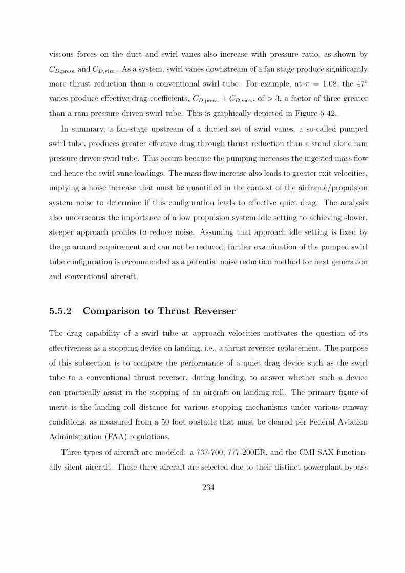
viscous forces on the duct and swirl vanes also increase with pressure ratio, as shown by
CD,press. and CD,visc.. As a system, swirl vanes downstream of a fan stage produce significantly
more thrust reduction than a conventional swirl tube. For example, at π = 1.08, the 47
vanes produce effective drag coefficients, CD,press. + CD,visc., of > 3, a factor of three greater
than a ram pressure driven swirl tube. This is graphically depicted in Figure 5-42.
In summary, a fan-stage upstream of a ducted set of swirl vanes, a so-called pumped
swirl tube, produces greater effective drag through thrust reduction than a stand alone ram
pressure driven swirl tube. This occurs because the pumping increases the ingested mass flow
and hence the swirl vane loadings. The mass flow increase also leads to greater exit velocities,
implying a noise increase that must be quantified in the context of the airframe/propulsion
system noise to determine if this configuration leads to effective quiet drag. The analysis
also underscores the importance of a low propulsion system idle setting to achieving slower,
steeper approach profiles to reduce noise. Assuming that approach idle setting is fixed by
the go around requirement and can not be reduced, further examination of the pumped swirl
tube configuration is recommended as a potential noise reduction method for next generation
and conventional aircraft.
5.5.2 Comparison to Thrust Reverser
The drag capability of a swirl tube at approach velocities motivates the question of its
effectiveness as a stopping device on landing, i.e., a thrust reverser replacement. The purpose
of this subsection is to compare the performance of a quiet drag device such as the swirl
tube to a conventional thrust reverser, during landing, to answer whether such a device
can practically assist in the stopping of an aircraft on landing roll. The primary figure of
merit is the landing roll distance for various stopping mechanisms under various runway
conditions, as measured from a 50 foot obstacle that must be cleared per Federal Aviation
Administration (FAA) regulations.
Three types of aircraft are modeled: a 737-700, 777-200ER, and the CMI SAX function-
ally silent aircraft. These three aircraft are selected due to their distinct powerplant bypass
234

ratios of about 5, 9, and > 15 during ground roll. A comparison is made between 1) brakes
alone, 2) brake plus a quiet drag device, and 3) brakes plus a thrust reverser. The results
of the study suggest that brakes alone can provide most of the stopping force on a dry or
wet runway, while a quiet drag device and a thrust reverser have a secondary effect. On a
slippery runway, i.e., an emergency situation when brakes are much less effective, the study
suggests that a thrust reverser is a much better stopping mechanism than a quiet drag device,
because a quiet drag device is not effective at low speeds. The majority of the effectiveness
of the thrust reverser comes from its ability to ingest a large streamtube of air to generate
ram drag. This leads to the recommendation to integrate variable vanes into a bypass or
mixing duct, to provide pumped swirl tube drag on approach. These vanes could then swivel
to a closed position on landing to serve the function of a thrust reverser blocker door.
Modeling Approach
The next subsection describes the various models employed in the stopping distance calcu-
lations.
Governing Equation. Newton’s second law on the aircraft is given by,
mlandingdV
dt= k0 + k1V + k2V
2, (5.20)
where the right hand side represents the various stopping mechanism forces. The aircraft
mass during landing is assumed constant during the event. The equation is solved using an
ordinary differential equation (ODE) solver, to obtain the time history of the aircraft landing
roll. The k coefficients are determined by the stopping mechanism models, as described
below.
Airframe Drag and Quiet Drag. A constant airframe drag coefficient is assumed in this
model. To this an additive quiet drag device coefficient is applied if one or multiple quiet
drag devices such as swirl tubes are employed. The quiet drag coefficient is assumed to be
235

1.00 based on throughflow area for simplicity. Overall throughflow area is set equal to the
total fan area of the propulsion system of each aircraft. Hence this type of drag is assumed
to be proportional to the square of the velocity, and both types of drag contribute to the k2
coefficient in Equation 5.20, i.e.,
Airframe and/or Quiet Drag ∝ V 2.
Braking. Rolling resistance braking coefficients are selected based on values published by
Raymer [70] and summarized in the Table 5.6, assuming the conservative scenario of worn
brakes performing at the lowest range of the published values.
The braking coefficient times the aircraft weight gives the stopping force, which is an
assumed constant that contributes to the k0 coefficient in Equation 5.20, i.e.,
Wheel Braking Force ∝ Constant.
Thrust Reverser. The thrust reverser is modeled as a device that has two drag generation
mechanisms, ram drag and reverse stream thrust drag. The operating point is defined by an
off-design gas turbine simulation model, GasTurb, for each engine type, to model the core,
fan, or mixed nozzle temperature and pressure ratios. The engine geometric parameters
then set the ingested mass flow and the ideal forward stream thrust that each engine stream
generates. The ram drag is the ingested mass of the fan stage times the aircraft velocity.
As thrust reverse is a high-power operating point where the pressure rise across the fan is
Scenario µbraking
Brakes Off, Wheels Rollng 0.03Brakes On, Dry Runway 0.30Brakes On, Wet Runway 0.15
Brakes On, Slippery/Icy Runway 0.06
Table 5.6: Braking coefficient summary reproduced from Raymer [70], assuming the conser-vative scenario of worn brakes.
236
much larger than the ram pressure rise, the ingested mass flow, m, based on static operation
at the selected engine setting is assumed constant during the landing event. The ram drag
then equals the product of m and the aircraft velocity. Since m is constant, it is equal to
the k1 coefficient in Equation 5.20 and
Ram Drag ∝ V.
The thrust reverser efficiency, ηtr, is a factor that multiplies the ideal forward stream
thrust as defined by Asbury et al. [3]. This product is the assumed reverse stream thrust
for either a mixed or fan stream. ηtr is set at 31% for the mixed flow exhaust thrust of
the CMI SAX functionally silent aircraft, and 54% of the separate flow fan stream exhaust
thrust on the 737 and 777 aircraft, based on published values [3]. The core streams on the
737 and 777 are modeled to generate forward thrust. As all streams are assumed choked
during thrust reverser operations, these thrust levels are assumed constant and contribute
to the k0 coefficient in Equation 5.20, i.e.,
Forward or Reverse Stream Thrust Force ∝ Constant.
Assumed Event Sequences
Assumed event sequences, shown below, are modeled per correspondence with a senior cap-
tain at easyJet airlines [62].
Dry and Wet Runway. These are assumed to be routine procedures for the pilot-in-
command.
1. The aircraft clears a 50 foot (15.24 meter) obstacle on a given glideslope angle and
flares at 5 meters altitude.
2. At t = 0 seconds, the rear wheels touch down (µRolling = 0.03).
237

3. At t = 3 seconds, the nose wheel is flown down. The rear brakes are auto-locked such
that µbraking=0.15.
4. At t = 5 seconds, the thrust reverser, if available, is engaged. During the transient
only ram drag is produced (to crudely average the spool up time with the steady state
reverse stream thrust). Brakes are assumed pilot-locked (µ = 0.30) below 100 knots
(51.4 meters/second).
5. At t = 11 seconds, the thrust reverser, if available, reaches steady state. A standard
reverser setting of 85% corrected engine speed (N1) is assumed for SAX, while 70%
corrected N1 is assumed for the 737 and 777. The thrust reverser is turned off below
60 knots (30.9 meters/second), to avoid the risk of re-ingesting hot gases into the fan
stream.
The same scenario applies to the wet runway except that the pilot locked braking coeffi-
cient is µ = 0.15. If present, a quiet drag device such as a ram pressure driven swirl tube is
assumed to provide drag during the entire event.
Slippery/Icy Runway. A slippery or icy runway is treated as an emergency scenario. It
is assumed that the pilot has situational awareness of the slippery runway, and is therefore
able to respond more rapidly than in a routine dry or wet runway scenario.
1. The aircraft clears a 50 foot (15.24 meter) obstacle on a given glideslope angle and
flares at 5 meters altitude.
2. At t = 0 seconds, the rear wheels touch down (µRolling = 0.03).
3. At t = 3 seconds, the nose wheel is flown down. The rear brakes are pilot-locked such
that µbraking=0.06. The thrust reverser, if available, is rapidly engaged. During the
transient only ram drag is produced (to crudely average the spool up time with the
steady state reverse stream thrust).
238

4. At t = 9 seconds, the thrust reverser, if available, reaches steady state. Maximum
reverse is applied as 85% corrected N1 for all aircraft types. The thrust reverser is
turned off below 20 knots (30.9 meters/second), trading the hot gas re-ingestion risk
for a shortened stopping distance.
Again, if present, a quiet drag device such as a ram pressure driven swirl tube is assumed
to provide drag during the entire event.
Runway Condition, Stopping Mechanism 737-700A 777-200ER SAX11Dry, Brakes Only 1144 1336 1399Dry, Brakes + Swirl Tube (CD = 1.00) 1120 1263 1304Dry, Brakes + Thrust Rev. 1063 1181 1197Wet, Brakes Only 1550 1734 1762Wet, Brakes + Swirl Tube (CD = 1.00) 1493 1655 1643Wet, Brakes + Thrust Rev. 1362 1458 1450Slippery, Brakes Only 3007 3393 3094Slippery, Brakes + Swirl Tube (CD = 1.00) 2767 3060 2710Slippery, Brakes + Thrust Rev. 1543 1550 1541Slippery, Brakes + Thrust Rev. (Ram Drag Only) −−−− −−−− 1976Published Landing Field Length (Janes) 1418 1616 −−−−
Table 5.7: Landing roll lengths in meters for various scenarios. Published values fromJane’s [44] included for comparison.
Results and Discussion
The primary figure of merit is the landing roll distance for various stopping mechanisms.
Table 5.7 presents the landing roll distances in meters for the three aircraft types considered
in this study. From the table, the important finding of this study is that on dry and wet
runways, braking alone absorbs the majority of the aircraft’s touchdown kinetic energy,
while on a slippery runway (an emergency scenario which is considered unsafe for normal
operation), a thrust reverser is the most effective stopping device. This finding is consistent
with data shown in Yetter [97].
In none of these conditions is a quiet drag device such as a ram pressure driven swirl tube
effective at significantly reducing stopping distance. Thus, a stand alone swirl tube would
239

0 500 1000 1500 2000 2500 30000
0.1
0.2
0.3
0.4
0.5
0.6
0.7
0.8
0.9
1
Distance (meters)
Vf/V
i
Airframe Drag +Wheel Brake
Airframe & Quiet Drag +Wheel Brake
Airframe Drag +Wheel Brake + Thrust Rev.
Airframe Drag + Wheel Brake +Thrust Rev. (Only Ram Drag)
Figure 5-43: SAX landing roll velocity vs. distance.
not be an effective a thrust reverser replacement. However, it should be noted that thrust
reversers are required by FAA regulations [97], and that airlines find them popular primarily
because they reduce brake wear and allow for shorter taxi times between the runway and
terminal.
In the case of a pumped swirl tube, achieved through deployable swirl vanes in a bypass
duct downstream of a fan stage, it may be possible to actuate the vanes to a closed position
on landing. This would serve the function of thrust reverser blocker doors. In this case
the quiet drag device could be integrated into a thrust reverser package, possibly mitigating
weight penalties associated with the actuating vanes. This concept is presented in Figure 4-6
as part of the earlier discussion on swirl tube configurations.
For the SAX BWB type aircraft with embedded, boundary layer ingesting (BLI) engines,
installation issues are non-trivial. Figure 5-43 shows a plot of ground velocity divided by
initial touchdown velocity versus landing distance measured from the 50 foot obstacle. Two
240

thrust reverser scenarios are shown, one with ram drag alone, requiring the ingested flow to
be dumped radially outwards, and one with a mixed exhaust reverse stream thrust model.
The computed stopping distances suggest that the CMI SAX embedded engine installation
could have many of the benefits of a thrust reverser, while possibly saving weight by dump-
ing flow radially only, by using the ram drag only option. This would require a nacelle
door to open above the embedded engine to dump flow upwards (perhaps the only prac-
tical direction for an embedded engine). It is recommended that this integration scenario
for a swirl tube/thrust reverser package be pursued in future designs of highly integrated
airframe/propulsion systems such as the final SAX design.
5.6 Summary of Major Findings
The major findings and key messages from this chapter may be summarized as:
1. A ram pressure driven swirl tube is a viable quiet drag device, because it can generate
high drag coefficient (0.83 measured at model-scale, estimated as 0.79 for full-scale,
1.2 meters diameter) with low noise signature. An A-weighted OASPL of 42 dBA
on approach is estimated, suggesting the device noise falls well below the background
noise of a well populated urban area.
2. A successful low-noise, high-drag swirl tube design achieves stable swirling flow as close
to but not exceeding the vortex breakdown threshold. Maximum flow angles at the
duct exit are close to 50.
3. Vortex breakdown is the limiting aerodynamic and aeroacoustic physical phenomenon
to swirl tube performance. Excessive swirl angle leads to breakdown, which reduces
drag and increases noise by about 15 dB at high frequencies.
4. Scaling laws and DAMAS source maps indicate that the noise signature of the preferred
swirl tube configuration (47) has both scattering and/or dipole-like sources near the
duct trailing edge and quadrupole-like volume sources in the swirling exhaust.
241

5. The swirl tube, as designed, generates greater effective drag when pumped by a fan
stage, because its ingested mass flow and vane loadings increases. The increased exit
velocity suggests a noise penalty. For the case of 47 swirl vanes, up to three times
greater effective drag occurs, at an estimated noise penalty of 24 dB. This suggests a
careful pumped swirl tube noise assessment as part of a system level noise assessment
is needed in future work.
6. Swirl tubes are not as effective as thrust reversers for landing on a slippery runway.
However, by actuating to a completely closed position, swirl vanes may be incorporated
into a thrust reverser package by serving as blocker doors on landing.
242

Chapter 6
Summary and Conclusions of the
Thesis
This chapter summarizes the research conducted and lists the contributions of the thesis. In
proposing two novel turbomachinery concepts, new areas of research are opened to further
exploration. This chapter also offers recommendations for future work to further the research
presented in this thesis.
6.1 Compressor Cooling
6.1.1 Summary of Research
Compressor cooling is motivated by the thermal management challenges associated with
low-to-high Mach number (0 to 4+) aircraft missions. The idea of heat extraction within the
blade passages of an axial compressor is conceived to improve performance, operability, and
durability of compressors, as well as improve the overall turbopropulsion cycle by combining
the function of a compressor and a heat exchanger.
The effect of blade passage surface heat extraction on axial compressor performance is
assessed with computational experiments and meanline modeling. At the blade passage level,
cooling improves blade-to-blade aerodynamic performance by:
243

1. lessening the total pressure reduction across the blade passage.
2. increasing the flow turning.
3. reducing the exit Mach number and total temperature, a potentially favorable scenario
for downstream blade rows.
The improvement in total pressure reduction from cooling is found to be comparable to
the Rayleigh line predicted result at low subsonic inlet Mach numbers (0.4), and greater
than this amount at high subsonic Mach numbers (0.8). Blade passage flow computations
provide the basis for generic bulk performance rules for a cooled compressor preliminary
design (meanline) framework. Single- and multi-stage compressor performance is modeled
at on- and off-design conditions. Pressure ratio and efficiency maps reveal that cooling inside
the blade passages of a compressor provides:
1. an increase in the overall pressure ratio (at a given corrected flow).
2. an increase in the maximum mass flow capability.
3. an increase in the efficiency, referenced to an adiabatic, reversible process.
4. rear stage choking relief at low corrected speed.
Results also suggest that, if available, a given amount of cooling is better in the front of
the compressor than in the rear. This is primarily a thermodynamic effect resulting from the
downstream stages compressing the colder air to a higher pressure ratio for a given amount of
work. For an adiabatically designed eight-stage compressor with pressure ratio of 5, results
suggest that heat extraction of 1% of inlet stagnation enthalpy flux in each of the first four
blade rows improves pressure ratio and efficiency by 23% and 15%, respectively, at design
corrected speed and mass flow. Choking mass flow is also found to improve by 5% at design
corrected speed.
Three-dimensional computations on a state-of-the art transonic rotor (NASA Rotor 35)
are shown to be in accord with the conclusions from the meanline analysis.
244

A preliminary heat transfer analysis reveals that the beneficial impact of blade passage
heat extraction is limited by available surface area and temperature difference. This favors
heat exchange in the rear stages of a compressor, and suggests the existence of an optimal
cooling scheme.
Finally, the primary efficiency metric presented in this thesis for comparison between
adiabatic and non-adiabatic compressors is referenced to an adiabatic, reversible process.
An alternate efficiency definition referenced to a non-adiabatic, reversible process is also
presented. The former efficiency metric is recommended for component-level comparisons,
while the latter may be appropriate as part of a system level analysis.
6.1.2 Summary of Contributions
Contributions from the compressor cooling research, as presented in Chapter 1, are repeated
here as a summary:
1. Assessment of the effects of heat extraction on blade passage performance metrics.
2. Development of a first-of-its-kind compressor meanline modeling framework with heat
extraction to assess the on- and off-design behavior of a cooled axial compressor.
3. Explanation of the causality between performance implications of heat extraction in
blade passage flows and the behavior of an axial compressor, including a CFD simula-
tion of a three-dimensional rotor passage of practical interest.
4. Establishment of new efficiency metrics for compressors with heat extraction, substan-
tiated by a bookkeeping of entropy generation from viscous and thermal dissipation.
6.1.3 Recommendations for Future Work
Unanswered questions regarding the feasibility of cooled compression turbopropulsion cycles
focus on the design requirements of a cooled compressor, and overall system performance
in terms of specific thrust capability, fuel burn and weight penalties. These tradeoffs must
245

be quantified in future work to determine whether the compressor cooling concept is worth
pursuing on a high speed flight vehicle, or other high temperature application such as a
modern turbofan with high overall pressure ratio. Several recommendations for future work
may be proposed in light of what is learned in this thesis.
Meanline modeling demonstrates that a given amount of cooling is favorable in the front
stages of a compressor, because the benefit is also felt by downstream stages. This competes
with the finding that higher heat transfer rates are achievable in the rear of the device, due
to higher temperatures and blade solidities. A study that warrants further consideration is
the optimization of a cooling scheme given these competing effects. This could be performed
at a component level, assuming some type of heat sink capability and heat exchange scheme.
A further step would be to optimize a cooling schedule over the course of a low-to-high Mach
number mission. This becomes a system level thermal management problem, that is mission
specific. A side-by-side comparison between a compressor- or hybrid- cooled turbojet cycle
and a pre-cooled turbojet cycle is a recommended first step.
At the blade-to-blade level, an experiment on a cooled cascade is warranted to study
different heat exchange schemes, as well as the effect of blade parameters such as the solidity,
pitch, and turning on non-adiabatic performance. An experimental design study would bring
to light the different challenges and tradeoffs involved in meeting the aerodynamic and heat
transfer requirements. If successful at the cascade level, a cooled stator experiment on a
compressor rig would be a logical next step. In addition, a compressor cooling scheme could
be incorporated into casing surfaces to extract heat from rotor passages. Heat extraction
across rotor blades would be the final and most challenging aspect of a cooled compressor,
for which unconventional turbomachinery heat exchanger concepts such as a multiphase
thermosyphon heat pipe may be explored.
Another potential compressor cooling study, numerical or experimental, would be to
use conventional axial compressor tip casing treatments, which can have cooling fin-like
structures that increase available surface area, for rotor blade passage cooling. This concept
may be an attractive application because these treatments are already in place in some
246

compressors to improve operability, but may provide additional surface area to increase the
available heat transfer rates.
6.2 Swirl Tube
6.2.1 Summary of Research
The concept of quiet drag is found to be a key enabler for a next-generation functionally
quiet aircraft on approach. Deployment of a quiet drag device in clean airframe configuration
offers the potential to reduce aircraft source noise and noise propagation to the ground. A
device that generates swirling outflow from a duct, such as an aircraft engine, is conceived
to have high drag and low noise. The simplest configuration is a ram pressure driven duct
with non-rotating swirl vanes, a so-called swirl tube. A swirl tube aerodynamic design is
performed using first principles and CFD computations, and validated through wind tunnel
aerodynamic and acoustic testing.
First principles preliminary modeling suggests a theoretical maximum drag coefficient
near 1.0 based on throughflow area. An inviscid, axisymmetric streamline curvature flow
solver provides swirl vane exit angles for a family of swirl tubes modeled as actuator disks
inside a nacelle and centerbody geometry. Three dimensional vanes are then designed to pro-
vide the proper turning. CFD computations complete the aerodynamic design by predicting
drag coefficients and the onset of the vortex breakdown phenomenon.
The swirl tube aerodynamic design is validated through model-scale wind tunnel exper-
iments. Flow visualization indicates that vortex breakdown occurs between cases with 47
and 57 swirl vane angle. Steady velocity measurements obtained from hot-wire traverses
show excellent agreement between CFD and experiment, in terms of axial and circumferen-
tial velocity profile, size and extent of viscous core, and computation of swirl angle. The
steady velocity measurements also show good qualitative agreement with the outer swirling
flow of the vortex breakdown cases, as well as the presence of breakdown in the core region.
Drag measurements validate the hypothesis that high drag coefficients (& 0.8) are achiev-
247

able, with the preferred design having 47 swirl vane angle with model-scale drag coefficient
of 0.83.
Swirl tube acoustics are experimentally assessed at the NASA Langley Quiet Flow Fa-
cility (QFF), a state-of-the art anechoic wind tunnel. Noise signatures are found to be
broadband for all swirl tubes, with a clear distinction between stable and vortex breakdown
outflows. Stable flows have broadband spectra that roll off at higher frequencies, while vortex
breakdown flowfield spectra closely resemble white noise at high frequencies. In addition,
vortex breakdown flowfield spectra are ∼ 15 dB louder than stable flows, demonstrating
that a high-drag, low-noise design exists for highly swirling flows that do not exceed the
vortex breakdown instability limit. When extrapolated to geometries of practical interest,
it is found that the noise from a swirl tube is significantly below the background noise of a
well populated area, demonstrating the viability of the swirl tube as a quiet drag device.
Propulsion system integration of swirl vanes downstream of a fan-stage, a so-called
pumped swirl tube is assessed using CFD. The effect of pumping is found to increase the
mass flow through the duct, providing large effective drag in the form of thrust reduction.
Higher exit velocities from pumping indicate the need to quantify the noise from a pumped
swirl tube. Finally, a recommendation is put forth to integrate swirl vanes into a thrust
reverser package, with the swirl vanes capable of actuating to a closed blocker door position.
6.2.2 Summary of Contributions
A swirl tube is a novel turbomachinery concept that is conceived and developed as a solution
to the clean airframe approach challenge for a next-generation, functionally quiet aircraft.
Research contributions identified in Chapter 1 are repeated here as a summary:
1. Successful demonstration of quiet drag coefficient of 0.8 with noise signature of 42 dBA
from a full-scale swirl tube.
2. Quantification of the relationship between swirl angle, drag, and noise for a family of
swirl tube designs.
248

3. Identification and quantification of acoustic sources associated with the swirling outflow
of a ram pressure driven swirl tube.
4. Identification of the limitations imposed by the vortex breakdown phenomenon on swirl
tube aerodynamic and acoustic performance.
5. Preliminary description of the propulsion-system integrated effect of a fan driven swirl
drag device for slow, steep approaches to reduce aircraft approach noise.
6. Recommendation to integrate swirl vanes into a thrust reverser system to achieve the
dual functionality of drag on approach and thrust reverser blocker doors during landing.
6.2.3 Recommendations for Future Work
This thesis presents a thorough assessment of the aerodynamic and acoustic performance of a
ram pressure drive swirl tube. This technology concept may thus be considered ready for the
next-level of feasibility study involving practical implementation challenges on an aircraft.
Mechanical design challenges for future work include deployment schemes in conventional and
drag generation modes. Location and design of ducting on an aircraft should be considered
by an aircraft manufacturer. Weight penalties associated with a ram air driven swirl tube
should also be quantified.
Additional drag potential is suggested by preliminary modeling and computations of a
pumped swirl tube. The acoustics of a pumped swirl tube should thus become the primary
focus of further research to determine if a high-drag, low-noise design space exists for such
a device. Fundamental experiments on highly swirling jet-like flows driven by approach idle
pressure ratios would determine the noise penalty associated with the increased velocities of
a pumped swirl tube exhaust. If successful, implementation of swirl vanes into an aircraft
engine could follow, with the additional mechanical feature of thrust reverser blocker door
capability.
Several different studies that were performed during the noise tests at the NASA Langley
QFF include the effect of aft centerbody shape and throughflow, inlet distortion, and angle of
249

attack. The data from these non-standard configurations should be dissected to shed further
light on the fundamental aerodynamic mechanisms that set the swirl tube noise signature.
Another important acoustics question would be whether the noise from a swirl tube could
be further reduced through acoustic treatments. If there are noise sources internal to the
swirl tube, as suggested by the DAMAS source maps, this may open the door for further
noise reduction in a ram pressure driven or pumped swirl tube. Liner design for swirling
flow should be investigated in this context.
250

Bibliography
[1] Agarwal, A. and A. P. Dowling. The Calculation of Acoustic Shielding of Engine Noise
by the Silent Aircraft Airframe. AIAA-2005-2996, 11th AIAA/CEAS Aeroacoustics
Conference, Monterrey, California, USA, May 23-25, 2005.
[2] Anderson, J. D. Introduction to Flight, 3rd Ed. McGraw-Hill Publishing Company, New
York, NY, 1989.
[3] Asbury, S.C and J.A. Yetter. Static Performance of Six Innovative Thrust Reverser
Concepts for Subsonic Transport Applications. Technical Memorandum 210300, NASA,
Langley, VA, 2000.
[4] Bearman, P.W. The Effect of Base Bleed on the Flow behind a Two-Dimensional Model
with a Blunt Trailing Edge. The Aeronautical Quarterly, 1967.
[5] Bragg, S.L. and W.R. Hawthorne. Some Exact Solutions of the Flow through Annular
Cascade Actuator Discs. Journal of the Aeronautical Sciences, 17, 1950.
[6] Brooke Benjamin, T. Theory of the Vortex Breakdown Phenomenon. Journal of Fluid
Mechanics, 1962.
[7] Brooks, T.F. Airfoil Self-Noise and Prediction. Reference Publication 1218, NASA,
Hampton, VA, 1989.
[8] Brooks, T.F. and M.A. Marcolini. Airfoil Tip Vortex Formation Noise. AIAA Journal,
1986.
251

[9] Brooks, T.F. and W.M. Humphreys Jr. Flap-edge Aeroacoustic Measurements and
Prediction. Journal of Sound and Vibration, 2003.
[10] Brooks, T.F. and W.M. Humphreys Jr. Three-Dimensional Application of DAMAS
Methodology for Aeroacoustic Noise Source Definition. AIAA-2005-2960, 11th
AIAA/CEAS Aeroacoustics Conference, Monterrey, California, USA, May 23-25, 2005.
[11] Brooks, T.F. and W.M. Humphreys Jr. A Deconvolution Approach for the Mapping of
Acoustic Sources (DAMAS) Determined from Phased Microphone Arrays. Journal of
Sound and Vibration, 2006.
[12] Brooks, T.F. and W.M. Humphreys Jr. Extension of DAMAS Phased Array
Processing for Spatial Coherence Determination (DAMAS-C). AIAA-2006-2654, 12th
AIAA/CEAS Aeroacoustics Conference, Cambridge, Massachusetts, USA, May 8-10,
2006.
[13] Clarke, J.B., N.T. Ho, L. Ren, J.A. Brown, K.R. Elmer, K. Tong and J.K. Wat. Con-
tinuous Descent Approach: Design and Flight Test for Louisville International Airport.
AIAA Journal of Aircraft, 2004.
[14] Cumpsty, N.A. Compressor Aerodynamics. Longman, Cambridge, UK, 1989.
[15] Darmofal, D.L., R. Khan, E.M. Greitzer and C.S. Tan. Vortex Core Behavior in Con-
fined and Unconfined Geometries: A Quasi-One-Dimensional Model. Journal of Fluid
Mechanics, 2003.
[16] Delery, J.M. Aspects of Vortex Breakdown. Progress in Aerospace Sciences, 1994.
[17] Diedrich, A., J. Hileman, D. Tan, K. Wilcox and Z. Spakovszky. Multidisciplinary De-
sign and Optimization of the “Silent” Aircraft. AIAA-2006-1323, 44th AIAA Aerospace
Sciences Meeting and Exhibit, Reno, Nevada, Jan. 9-12, 2006, 2006.
[18] Dowling, A.P. and J.E. Ffowcs Williams. Sound and Sources of Sound. Ellis Horwood
Limited, Chichester, UK, 1983.
252

[19] Drela, M. Two-Dimensional Transonic Aerodynamic Design and Analyis Using the
Euler Equations. Report 187, MIT Gas Turbine Laboratory, Cambridge, MA, 1986.
[20] Drela, M. A User’s Guide to MTFLOW 1.2 - Multi-passage throughFLOW De-
sign/Analysis Program. November 1997 1997.
[21] Engineering Sciences Data Unit. ESDU 81009: Estimation of Windmilling Drag and
Airflow of Turbo-jet and Turbo-fan Engines, 1981.
[22] Federal Aviation Administration. Federal Aviation Regulations, Part 25 Section 125.
FAA Document, August 2006.
[23] Fluent, Inc., Lebanon, NH. Fluent 6.1 User’s Guide, 2003.
[24] Goldstein, M.E. Aeroacoustics. McGraw-Hill, New York, NY, 1976.
[25] Goldstein, M.E. Ninety Degree Acoustic Spectrum of a High-Speed Air Jet. AIAA
Journal, 2005.
[26] Gong, Y., B.T. Sirakov, A.H. Epstein and C.S. Tan. Aerothermodynanics of micro-
turbomachinery. ASME GT2004-53877, 2004.
[27] Greitzer, E.M, C.S. Tan and M.B. Graf. Internal Flow Concepts and Applications.
Cambridge University Press, Cambridge, UK, 2004.
[28] Hall, M.G. Vortex Breakdown. Annual Review of Fluid Mechanics, 1972.
[29] Harada, K., N. Tanatsugu and T. Sato. Development Study of a Precooler for the
Air-Turboramjet Expander-Cycle Engine. Journal of Propulsion and Power, 2001.
[30] Harvey, J.K. Some Observations of the Vortex Breakdown Phenomenon. Journal of
Fluid Mechanics, 1962.
[31] Heiser, W.H. and D.T. Pratt. Hypersonic Airbreathing Propulsion. AIAA, Washington,
DC, 1994.
253

[32] Hewitt, F.A. and M.C. Johnson. Propulsion System Performance and Integration for
High Mach Air Breathing Flight. In S.N.B. Murthy and E.T. Curran, editors, High
Speed Flight Propulsion Systems, volume 137. AIAA, 1991.
[33] Hileman, J., Z. Spakovszky, M. Drela and M. Sargeant. Aerodynamic and Aeroa-
coustic Three-Dimensional Design for a “Silent” Aircraft. AIAA-2006-241, 44th AIAA
Aerospace Sciences Meeting and Exhibit, Reno, Nevada, Jan. 9-12, 2006.
[34] Horlock, J.H. Acutator Disk Theory. McGraw-Hill, London, UK, 1978.
[35] Howe, M.S. A Review of the Theory of Trailing Edge Noise. Journal of Sound and
Vibration, 1978.
[36] http://www.boeing.com.
[37] http://www.princeton.edu/∼stengel/MAE331.html.
[38] http://www.sengpielaudio.com/TableOfSoundPressureLevels.htm.
[39] Hubbard, H.H. and J.C. Manning. Aeroacoustic Research Facilities at NASA Langley
Research Center: Description and Operational Characteristics. Technical Memorandum
TM-84585, NASA, Hampton, VA, 1983.
[40] Humphreys, W.M., T.F. Brooks, W.H. Hunter, and K.R. Meadows. Design and Use of
Microphone Directional Arrays for Aeroacoustic Measurements. AIAA-1998-0471, 36th
Aerospace Sciences Meeting and Exhibit, Reno, Nevada, USA, January 12-15, 1998.
[41] Hutcheson, F.V. and T.F. Brooks. Measurement of Trailing Edge Noise Using Direc-
tional Array and Coherent Output Power Methods. AIAA-2002-2472, 8th AIAA/CEAS
Aeroacoustics Conference, Breckenridge, Colorado, USA, June 17-19, 2002.
[42] Hutcheson, F.V. and T.F. Brooks. Noise Radiation from Single and Multiple Rod Con-
figurations. AIAA-2006-2629, 12th AIAA/CEAS Aeroacoustics Conference, Cambridge,
Massachusetts, USA, May 8-10, 2002.
254

[43] Isomura, K. and J. Omi. A Comparative Study of an ATREX Engine and a Turbo Jet
Engine. AIAA/ASME/SAE/ASEE 37th Joint Propulsion Conference, 2001.
[44] Jane’s Information Group, Coulsdon, Surrey, UK. Jane’s All the World’s Aircraft, 2005.
[45] Jenkins, D.R. Space Shuttle: The History of the National Space Transportation System.
Dennis R. Jenkins, Cape Canaveral, FL, 2002.
[46] Johnson, J.E. Variable Cycle Engine Developments. In Murthy, S.N.B. and E.T. Curran,
editor, Developments in High-Speed-Vehicle Propulsion Systems, volume 165. AIAA,
1995.
[47] Kerrebrock, J.L. Aircraft Engines and Gas Turbines, 2nd Ed. MIT Press, Cambridge,
MA, 1992.
[48] Leibovich, S. The Structure of Vortex Breakdown. Annual Review of Fluid Mechanics,
1978.
[49] Lighthill, M.J. On Sound Generated Aerodynamically. I. General Theory. Proceedings
of the Royal Society of London A, 1952.
[50] Lighthill, M.J. On Sound Generated Aerodynamically. II. Turbulence as a Source of
Sound. Proceedings of the Royal Society of London A, 1953.
[51] Lilley, G.M. The Prediction of Airframe Noise and Comparison With Experiment.
Journal of Sound and Vibration, 2001.
[52] Lockard, D.P. and G.M. Lilley. The Airframe Noise Reduction Challenge. Reference
Publication 213013, NASA, Hampton, VA, 2004.
[53] Manneville, A. Propulsion System Concepts for Silent Aircraft. Master’s thesis, MIT,
May 2004.
255

[54] Manneville, A., D. Pilczer and Z. S. Spakovszky. Preliminary Evaluation of Noise
Reduction Approaches for a Functionally Silent Aircraft. AIAA Journal of Aircraft,
2006.
[55] Manneville, A., D. Pilczer and Z. Spakovszky. Noise Reduction Assessments and
Preliminary Design Implications for a Functionally-Silent Aircraft. AIAA-2004-2925,
10th AIAA/CEAS Aeroacoustics Conference, Manchester, United Kingdom, May 10-12,
2004.
[56] Meadows, K.R., T.F. Brooks, W.M. Humphreys Jr., W.W. Hunter, and C.H. Ger-
hold. Aeroacoustic Measurements of a Wing-Flap Configuration. AIAA-1997-1595, 3rd
AIAA/CEAS Aeroacoustics Conference, Atlanta, Georgia, USA, May, 1997.
[57] Mendoza, J.M., T.F. Brooks, and W.M. Humphreys Jr. Aeroacoustic Measurements of a
Leading Edge Slat Configuration. International Journal of Aeroacoustics, 1(3):241–274,
2002.
[58] Mendoza, J.M., T.F. Brooks, and W.M. Humphreys Jr. Aeroacoustic Measurements
of a Wing-Slat Model. AIAA-2002-2604, 8th AIAA/CEAS Aeroacoustics Conference,
Breckenridge, Colorado, USA, June 17-19, 2002.
[59] Miele, A. Flight Mechanics, Volume 1: Theory of Flight Paths. Addison-Wesley Pub-
lishing Company, Reading, MA, 1962.
[60] Mizobata, K., H. Kimura, H. Sugiyama, T. Sato and H. Kobayashi. Conceptual Design
of Flight Demonstrator Vehicles for the ATREX Engine. AIAA/NAL-NASDA-ISAS
12th International Space Planes and Hypersonic Systems and Technologies Conference,
Norfolk, VA, 2003.
[61] Mobed, D. Aero-Acoustics of Swirling Flows for Drag Applications. Master’s thesis,
MIT, December 2006.
[62] Moody, S. Personal communication, 2005.
256

[63] Morris, P.J., and F. Farassat. Acoustic Analogy and Alternative Theories for Jet Noise
Prediction. AIAA Journal, 2002.
[64] Panton, R.L. Incompressible Flow. John Wiley and Sons, New York, NY, 1984.
[65] Pilczer, D. Noise Reduction Assessments and Preliminary Design Implications for a
Functionally Silent Aircraft. Master’s thesis, MIT, June 2003.
[66] Powell, T.H. and M.R. Glickstein. Precooled Turbojet Engine Cycle For High Mach
Number Applications. AIAA/SAE/ASME/ASEE 24th Joint Propulsion Conference,
1988.
[67] Quayle, A. Personal communication, 2006.
[68] Quayle, A., A. Dowling, H. Babinsky, and W. Graham. Landing Gear for a Silent
Aircraft. AIAA-2007-231, 45th Aerospace Sciences Meeting and Exhibit, Reno, Nevada,
USA, To Be Presented: January 8-11, 2007.
[69] Raizada, N. and P.J. Morris. Prediction of Noise from High Speed Subsonic Jets Using
and Acoustic Analogy. AIAA-2006-2596, 12th AIAA/CEAS Aeroacoustics Conference,
Cambridge, Massachusetts, USA, May 8-10, 2006.
[70] Raymer, D.P. Aircraft Design: A Conceptual Approach. AIAA Education Series, Reston,
VA, 1999.
[71] Reid, L. and R.D. Moore. Performance of Single-Stage Axial-Flow Transonic Compres-
sor With Rotor and Stator Aspect Ratios of 1.19 and 1.26, Respectively, and With
Design Pressure Ratio of 1.82. Technical Paper 1338, NASA, Cleveland, OH, 1978.
[72] Reynolds, T.G., L. Ren, J.B. Clarke, A.S. Burke and M. Green. History, Development
and Analysis of Noise Abatement Arrival Procedures for UK Airports. AIAA-2005-7395,
AIAA 5th Aviation, Technology, Integration and Operations Conference, Arlingont, Vir-
ginia, USA, September 26-28, 2005.
257

[73] Rudakov, A.S. and V.V. Balepin. Propulsion Systems with Air Precooling for Aerospace-
plane. SAE Paper 911182, 1991.
[74] Sarpkaya, T. On Stationary and Travelling Vortex Breakdown. Journal of Fluid Me-
chanics, 1971.
[75] Sato, T., N. Tanatsugu, H. Hatta, K. Goto, H. Kobayashi, J. Omi and J. Tomike. Devel-
opment Study of the ATREX Engine for TSTO Spaceplane. AIAA/NAL-NASDA-ISAS
10th International Space Planes and Hypersonic Systems and Technologies Conference,
Kyoto, Japan, 2001.
[76] Sawai, S., T. Sato, H. Kobayashi, N. Tanatsugu and H. Ohtsuka. Flight Test Plan
for ATREX Engine Development. AIAA/NAL-NASDA-ISAS 12th International Space
Planes and Hypersonic Systems and Technologies Conference, Norfolk, VA, 2003.
[77] Schlichting, A.H. Boundary Layer Theory. McGraw Hill, New York, 1987.
[78] Schumm, M., E. Berger and P.A. Monkewitz. Self-excited Oscillations in the Wake of
Two-dimensional Bluff Bodies and Their Control. Journal of Fluid Mechanics, 1994.
[79] Sevilla, A. and C. Martınez-Bazan. Vortex Shedding in High Reynolds Number Axisym-
metric Bluff-body Wakes: Local Linear Instability and Global Bleed Control. Physics
of Fluids, 2004.
[80] Shapiro, A.H. The Dynamics and Thermodynamics of Compressible Fluid Flow. Ronald
Press, New York, 1953.
[81] Smith, M.J.T. Aircraft Noise. Cambridge University Press, Cambridge, UK, 1989.
[82] Society of Automotive Engineers. SAE ARP876D: Gas Turbine Jet Exhaust Noise
Prediction, 1994.
[83] Squire, H.B. Analysis of the ‘Vortex Breakdown’ Phenomenon. Report 102, Imperial
College, London, Aeronautics Department, 1960.
258

[84] Sreenath, A.V. Studies of Turbojet Engines for Hypersonic Propulsion. Technical report,
McGill University, Department of Mechanical Engineering, 1961.
[85] Stone, J.R., D.E. Groesbeck and C.L. Zola. Conventional Profile Coaxial Jet Noise
Prediction. AIAA Journal, 1983.
[86] Taguchi, H., T. Sato, H. Kobayashi, T. Kojima, K. Okai, K. Fujita, T. Ohta. Design
Study on a Small Pre-Cooled Turbojet Engine for Flight Experiments. AIAA/NAL-
NASDA-ISAS 13th International Space Planes and Hypersonic Systems and Technolo-
gies Conference, 2005.
[87] Tam, C.K.W. Jet Noise: Since 1952. Theoretical and Computational Fluid Dynamics,
1998.
[88] Tam, C.K.W. and L. Auriault. Mean Flow Refraction Effects on Sound Radiated from
Localized Sources in a Jet. Journal of Fluid Mechanics, 1998.
[89] Tam, C.K.W. and L. Auriault. Jet Mixing Noise from Fine-Scale Turbulence. AIAA
Journal, 1999.
[90] Tam, C.K.W., and N. Pastouchenko. Noise from the Fine Scale Turbulence of Nonax-
isymmetric Jets. AIAA-2001-2187, 7th AIAA/CEAS Aeroacoustics Conference, Maas-
tricht, Netherlands, May 28-30, 2001.
[91] Tam, C.K.W., M. Golebiowski, and J.M. Seiner. On the Two Components of Turbulent
Mixing Noise from Supersonic Jets. AIAA Paper 96-1716, 1996.
[92] Tam, C.K.W., N. Pastouchenko and K. Vishwanathan. Fine-Scale Turbulence Noise
from Hot Jets. AIAA Journal, 2005.
[93] Tanatsugu, N., T. Sato, V. Balepin, Y. Naruo, T. Mizutani, T. Kashiwagi, K. Hamabe,
J. Tomike and R. Minami. Development Study on ATREX Engine. Acta Astronautica,
41(12), 1997.
259

[94] Tanna, H.K. On the Effect of Motion of Sources on Subsonic Jet Noise. Journal of
Sound and Vibration, 1973.
[95] Thies, A.T. and C.K.W. Tam. Computation of Turbulent Axisymmetric and Nonax-
isymmetric Jet Flows Using the K-epsilon Model. AIAA Journal, 1996.
[96] Wood, C.J. Visualization of an Incompressible Wake with Base Bleed. Journal of Fluid
Mechanics, 1967.
[97] Yetter, J.A. Why Do Airlines Want and Use Thrust Reversers? Technical Memorandum
109158, NASA, Langley, VA, 1995.
[98] Zweifel, O. The Spacing of Turbomachine Blading, Especially with Large Angular
Deflection. Brown Boveri Review, 32(12), 1945.
260