nonparametric econometrics - wise.xmu.edu.cn ullah—method i.pdf · correlations, earning...

Nonparametric Econometrics

Methods I

Aman Ullah

University of California, Riverside

A.Ullah (UCR) NP slides 1 / 54

Books

A. Pagan and A. Ullah, Nonparametric Econometrics, CambridgeUniversity Press, 1999.

Q. Li and J. Racine, Nonparametric Econometrics: Theory andPractice, Princeton University Press, 2007.

D. Henderson and C.F. Parmeter, Applied NonparametricEconometrics, Cambridge University Press, 2015.

J. Fan and I. Gilbels, Local Polynomial Modelling and ItsApplications, Chapman and Hall, 1996.

B.W. Silverman, Density Estimation for Statistics and DataAnalysis, Chapman and Hall, 1986.

B.L.S. Prakasa-Rao, Nonparametric Functional Estimation,Academic Press, 1983.

A.Ullah (UCR) NP slides June 23, 2015 2 / 54

Survey Papers

Zongwu Cai and Yongmiao Hong, Some Recent Developments inNonparametric Finance, Advances in Econometrics (Racine and Li),2009.

Zongwu Cai and Jingping Gu and Qi Li, Some Recent Developmentson Nonparametric Econometrics, Advances in Econometrics (Racineand Li), 2009.

J. Racine and A. Ullah, Nonparametric Econometrics, PalgraveHandbook of Econometrics (Mills and Patterson), PalgraveMacmillan, 2006.

J.L. Powell, Estimation of Semiparametric Models, Handbook ofEconometrics, Vol. IV (Engle and MaFadden), 1994.


Topics

1 Kernel Estimation of Density2 Conditional Mean (Regression)3 Time Series Conditional Variance (Volatility) and ConditionalCorrelations

4 Nonparametric Hypothesis Testing5 Semiparametric Models6 Empirical Examples: Financial Time Series Models of Volatility andCorrelations, Earning Functions, Income Distributions, Panel Data


Softwares

R-program

http://www.r-project.org/

Racine ’np’, ’npRmpi’, ’crs’ packages available from above link.

Eviews,Stata


Functions (Models) in Econometrics

{Y ,X},

Y = E (Y |X ) + U= m(X ) + U

f (X ), f (Y ), f (X ,Y ), f (Y |X )m(X ) = E (Y |X = x) : REGRESSION FUNCTION

b(x) = ∂m(x )∂x : REGRESSION COEFFICIENT FUNCTION

C (x) = ∂2m(x )∂x 2 : CURVATURE FUNCTION

s2(x) = V (Y |X = x) : VARIANCE (VOLATILITY)sY ,Z (x) = cov(Y ,Z |X = x) : COVARIANCE FUNCTIONLIKELIHOOD FUNCTION, SCORE FUNCTION


Distribution Function-Parametric

X : logwage

f (x) =1

sp2pe−

12 (

x−µs )2

{Xi}, i = 1, 2, ..., n

f (x) =1

sp2pe−

12 (

x−µs )2

µ = x = 1n Â xi ; s2 = 1

n Â(xi − x)2

Calculate for each x1, x2, ..., xn.


Distribution Function-Nonparametric [Data Based]

f (x) =1nh

n

Âi=1K (xi − x)

K (xi − xh

) = I (xi − xh

) = 1 if −12≤xi − xh

≤12

= 0 if otherwise

f (x) =number of data xi in [xi − h

2 , x +h2 ]

nh=n∗

nh= per unit relative frequency (proportion)


Distribution Function-Nonparametric [Data Based]

Empirical Density (Local Histogram): Jumps at the end of interval and 0derivatives elsewhere.


Smooth Density

(i) K ( xi−xh ) = 1p2pe−

12 (

xi−xh )2, −• < xi−x

h < •(ii) K ( xi−xh ) = 3

4 [1− (xi−xh )2],

∣∣ xi−xh

∣∣ ≤ 1

K ( xi−xh ) " if xi−xh "; K ( xi−xh ) # if xi−xh #h = sx n−1/51/06, 1.06sx n−1/(k+4).


PROPERTIES

Assumptions (p.21)1. i .i .d .2. f (x) is continuous and bounded3. Second order Kernel:RK (y)dy = 1,

RyK (y)dy = 0,

Ry2K (y)dy = µ2 < 0

4. h! 0, nh! • as n! •

BIAS(f (x)) =h2

2f (2)(x)µ2 = O(h

2)

V (f (x)) =1nhf (x)

ZK 2(y)dy = O(

1nh)

Theorem 2.2, p.23.


PROPERTIES

MSE (f (x)) = (BIAS)2 + V (f (x))

IMSE = MISE =Z

xMSE (f (x))dx (2.46)

=Z

x(BIAS)2dx +

Z

xV (f (x))dx

hopt = cn−15 (2.49)

c = [

RK 2(y)dy

µ22R(f (2)(x))2dx

]1/5

f (x)! N(µ, s2x ), K (y)! N(0, 1)c = 1.06sx

2-step (plug-in): c = c , substitute f (2)(x) for f (2)(x)Kopt = K (y) = 3

4 (1− y2); −1 ≤ y ≤ 1 (2.61).A.Ullah (UCR) NP slides June 23, 2015 13 / 54

CROSS-VALIDATION

p.51

minc

Z

x(f (x)− f (x))2dx

= mincISE

= minc[Z

xf 2(x)dx −

2nh(n− 1) Â

iÂj 6=iK (xj − xih

)]

where h = cn−1/5.


MULTIVARIATE

X : f (x)dx = f (x)h = 1n Ân

i=1 K (xi−xh )

X1 : f (x1)dx1 = f (x1)h = 1n Ân

i=1 K (x1i−x1h )

X1,X2 : f (x1, x2)dx1dx2 = f (x1, x2)h2 = 1n Ân

i=1 K (x1i−x1h , x2i−x2h )

X = [X1,X2, ...,Xq ]; x = (x1, x2, ..., xq)

f (x1, x2, ..., xq)hq = f (x)hq = 1n Ân

i=1 K (x1i−x1h , x2i−x2h , ...,

xqi−xqh ) or

f (x) =1nhq

n

Âi=1K (xi − xh

).


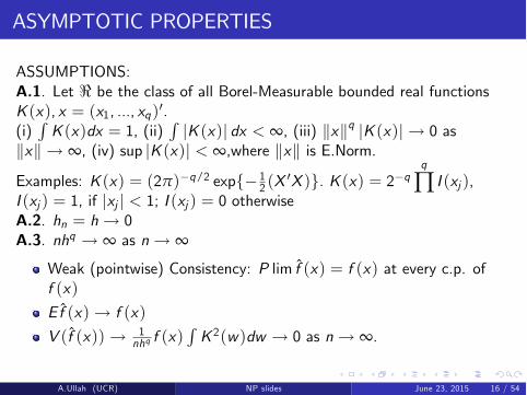
ASYMPTOTIC PROPERTIES

ASSUMPTIONS:A.1. Let < be the class of all Borel-Measurable bounded real functionsK (x), x = (x1, ..., xq)0.(i)RK (x)dx = 1, (ii)

R|K (x)| dx < •, (iii) kxkq |K (x)|! 0 as

kxk ! •, (iv) sup |K (x)| < •,where kxk is E.Norm.

Examples: K (x) = (2p)−q/2 exp{− 12 (X

0X )}. K (x) = 2−qq

’ I (xj ),I (xj ) = 1, if |xj | < 1; I (xj ) = 0 otherwiseA.2. hn = h! 0A.3. nhq ! • as n! •

Weak (pointwise) Consistency: P lim f (x) = f (x) at every c.p. off (x)

E f (x)! f (x)

V (f (x))! 1nhq f (x)

RK 2(w)dw ! 0 as n! •.


ASYMPTOTIC NORMALITY

pnhq(f (x)− f (x)− B) ∼ N(0, f (x)

ZK 2(y)dy)

where B = h22 µ2f

(2)(x),pnhh2 ! 0 as n! •; 95% C.I. for f (x) :

f (x)± 1.96qV (f (x)).

"CURSE OF DIMENSIONALITY "


Reduction in Bias (Higher Order Kernels)

If K 2 <r are kernels which could take negative/positive values such thatfirst (r − 1) moments are zero.Earlier case was r = 2.

Bias(f (x)) = O(hr ), Bias(M(x)) = O(hr ).

MSE (f (x)) = O(H2r ) +O( 1nhq ) where h µ n−1/(2r+q). Same for m(x).

MSE = O(n−2r/(2r+q))! O(n−1), if r is large.


f (x) = 1nh Ân

i=1 K (xi−xh ) = 1

nh Âni=1 K (yi ) where yi =

xi−xh ,

∣∣∣ dxdyi

∣∣∣ = h.1.

Z

xf (x)dx =

1nh

n

Âi=1

Z

xK (xi − xh

)dx

=1nh

n

Âi=1

Z

yi

K (yi )hdyi

=1n

n

Âi=11

= 1.


2. f (x) = 1n Ân

i=1 zi , zi =1hK (

xi−xh ).

E f (x) = Ez1

=1h

Z

x1K (x1 − xh

)f (x1)dx1

=Z

yK (y)f (x + hy)dy

=Z

yK (y)[f (x) + hyf (1)(x) +

h2y2

2f (2)(x) + · · · )dy

' f (x) +h2

2µ2f

(2)(x).


V (f (x)) =1n2

n

Âi=1V (zi )

=V (z1)n

=1n[Ez21 − (Ez1)

2]

=1n

Z 1h2K 2(

x1 − xh

f (x1)dx1)−1n(Ez1)2

=1nh

Z

yK 2(y)f (x + hy)dy−

1n(Ez1)2

'1nhf (x)

Z

yK (y)dy.


Cumulative Distribution Function

F (x) =Z x

−•f (t)dt

=Z x

−•

1nh

n

Âi=1K (t − xih

)dt

=1n

n

Âi=1

Z x

−•

1hK (t − xih

)dt.

Let t−xih = yi .

F (x) =1n

n

Âi=1

Z x−xih

−•K (yi )dyi

=1n

n

Âi=1G (x − xih

)

and G (z) =R z−• K (y)dy.


Cumulative Distribution Function

EF (x) = EG (x − xih

) =Z •

−•G (x − xih

)f (xi )dxi

= hZ •

−•G (z)f (x − hz)dz = −

Z •

−•G (z)dF (x − hz)

= −[G (z)F (x − hz)]•−• +Z •

−•K (z)F (x − hz)dz

=Z •

−•K (z)F (x − hz)dz

=Z •

−•K (z)[F (x)− F (1)hz +

12h2z2F (2)(x) + · · · ]dz

= F (x) +12

µ2h2F (2)(x) + o(h2)

' F (x) +12

µ2h2F (2)(x)

where x−xih = z . Thus, BIAS(F (x)) = 1

2µ2h2F (2)(x).


SIMILARITY

Let z = x−xih ,

EG 2(x − xih

) =Z •

−•G 2(

x − xih

)f (xi )dxi

= hZ •

−•G 2(z)f (x − hz)dz

= −Z •

−•G 2(z)dF (x − hz)

= 2Z •

−•G (z)K (z)F (x − hz)dz

= 2Z •

−•G (z)K (z)[F (x)− hzF (1)(x)]dz +O(h2)

= F (x)− lhf (x) +O(h2),

l = 2RzG (z)K (z)dz and

2R •−• G (z)K (z)dz =

R •−• dG

2(z) = G 2(•)− G 2(−•) = 1


V (F (x)) =1nV [G (

x − xih

)]

=1n[EG 2(

x − xih

)− (EG (x − xih

))2]

=1nF (x)(1− F (x))−

lf (x)hn

+ o(hn).

Hence

MSE (F (x)) '1nF (x)(1− F (x)) + h4(

µ22)2(F (2)(x))2 − lf (x)

hn

IMSE (F (x)) =Z

xMSE (F (x))2dx '

l1n−

l2hn+ l3h4

where h0 = l0n−1/3, l0 = (l2/l3)1/3 andpn(F (x)− F (x)) ∼ N(0,F (x)(1− F (x))).

Stochastic Dominance: Linton, Whang, Maasoumi (2005, RES).


TESTING

H0 : f (x) = g(x), H1 : f (x) 6= g(x)TEST STATISTIC

I =Z

x(f (x)− g(x))2dx ∼ N(0,V ) under H0

H0 : f1(x) = f2(x); Panel DataH0 : f (x) = f (−x) SymmetryH0 : f (y , x) = f (x)f (y), f (z) = g(z)H0 : f (x) = f (x , q).

Fan and Ullah (1998, JNS), Su and White (2008, ET; 2007, JE).


WHAT IS THE "TRUE" MODEL FOR THIS DATA?

THIS IS THE SUBJECT OF NONPARAMETRIC ECONOMETRICS(DATA BASED MODELING).

a+ X b : PARAMETRIC MODEL.


NONPARAMETRIC REGRESSION (CH.3)

(1) {Y ,X},X 2 R 0 Data {yi , xi}, i = 1, 2, ..., n

m(x) = E (Y |X = x) =Z

yyf (y |x)dy =

Z

yyf (y , x)f (x)

dy

m(x) =Z

yyf (y , x)

f (x)dy

=Z

yy

1nh2 Ân

i=1 K (yi−yh )K ( xi−xh )

1nh Ân

i=1 K (xi−xh )

dy

=Âni=1 yiK (

xi−xh )

Âni=1 K (

xi−xh )

NADARAYA/WATSON (1964, SANKHYA)


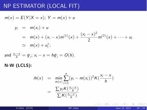
NP ESTIMATOR (LOCAL FIT)

m(x) = E (Y |X = x); Y = m(x) + u

yi = m(xi ) + u

= m(x) + (xi − x)m(1)(x) +(xi − x)2

2m(2)(x) + · · ·+ ui

' m(x) + u∗i ;

and xi−xh = yi ; xi − x = hyi = O(h).

N-W (LCLS):

m(x) = minm(x )

n

Âi=1(yi −m(xi ))2K (

xi − xh

)

=Â yiK ( xi−xh )

ÂK ( xi−xh )


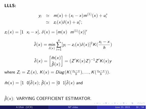
LLLS:

yi ' m(x) + (xi − x)m(1)(x) + u∗i' zi (x)d(x) + u∗i ;

zi (x) = [1 xi − x ], d(x) = [m(x) m(1)(x)]0

d(x) = mind(x )

n

Âi=1[yi − zi (x)d(x)]2K (

xi − xh

)

d(x) =[m(x)

b(x)

]= (Z 0K (x)Z )−1Z 0K (x)y

where Zi = Zi (x), K (x) = Diag(K ( x1−xh ), ....,K ( xn−xh )).

m(x) = [1 0]d(x); b(x) = [0 1]d(x) and

b(x): VARYING COEFFICIENT ESTIMATOR.


MISSPECIFICATION TEST

H0 : Y = a+ X b+ u or y = m(x , q) + uH1 : y = m(x) + u

) H0 : E (u|x) = 0; H1 : E (u|x) 6= 0

H0 : E (u|x) = 0) E [uE (u|x)] = 0) E [um∗(x)] = 0) E [um∗(x)f (x)] = 0


TEST STATISTIC

I =1n

n

Âi=1uim∗(xi )f (xi )

=1n

n

Âi=1ui m∗(xi )f (xi )

=1

n(n− 1)h

n

Âi=1

n

Âj 6=ij=1

ui ujK (xj − xih

) ∼ N(0,V ∗)

Li-Wang (J. Econometrics, 1998).


LLLS ESTIMATION OF VARYING (FUNCTIONAL)COEFFICIENTS

LLLS: Â(yi − xi b(x))2K ( xi−xh )

b(x) = (X 0K (x)X )−1X 0K (x)y

yi = xi b(zi ) + ui = m(xi ,zi ) + ui

Â(yi − xi b(z))2K ( zi−zh )

b(z) = (X 0K (z)X )−1X 0K (z)y


Examples: Parametric Models

THRESHOLD AR (TAR): TONG (90)

yi = yi−1b(yi−d ) + ui

b(yi−d ) = b1 if |yi−d | ≥ c= b2 if |yi−d | < c

b(yi−d ) = b1I (|yi−d | ≥ c) + b2I (|yi−d | < c)


WINDOW-WIDTH

CROSS-VALIDATION

yi = m(xi ) + ui

Min.Â u2i with respect to h

Also CV for both h and p ( local polynomial degree)Hall and Racine ( 2015, JE).

m(xi ) = m(x)+ (xi − x)m(1)(x)+ (xi − x)2m(2)(x)+ · · ·+(xi − x)pm(p)(x)


LLLS PROPERTIES

pnhq(m(x)−m(x)− B(x)) ∼ N(0,

s2(x)f (x)

Z

yK 2(y)dy)

where B(x) = 12µ2h

2m(2)(x).

pnhq+2(b(x)− b(x)− B1(x)) ∼ N(0,

s2(x)f (x)

Z

y(K (1)(y))2dy)

where B1(x) = 12µ2h

2m(3)(x).


QUANTILE ESTIMATION

yi = xi b+ ui

Â |ui | = Â |yi − xi b| = Âui≥0

ui − Âui≤0

ui

= Âui≥0

|ui |+ Âui≤0

|ui |

= Â ui I (ui ≥ 0)−Â ui I (ui < 0)

= Â ui (1− I (ui < 0))−Â ui I (ui < 0)

= Â ui (1− 2I (ui < 0)) = Â ui (0.5− I (ui < 0))

= Âui≥0

|ui |12+ Âui≤0

|ui |12

= Âui≥0

|ui | q + Âui≤0

|ui | (1− q)

! q·quantile


QUANTILE ESTIMATION

q−th quantile of FY = P(Y ≤ y), qY (q) is the solution of

P(Y ≤ y) = FY (q) = q =Z q

−•f (y)dy

qY (q) = F−1Y (q)

qEy>q |y − q|+ (1− q)Ey<q |y − q| =qRy>q |y − q| dFY (y) + (1− q)

Ry<q |y − q| dFY (y)

DWR to q = qZ

y>q(y − q)dFY (y) + (1− q)

Z

y<q(y − q)dFY (y)

0 = −qZ

y>qdFY (y) + (1− q)

Z

y<qdFY (y)

= −q[1− FY (q)] + (1− q)FY (q)

= −q + FY (q)


QUANTILE REGRESSION

(1) y = E (y |x) + u; y = a+ X b+ u, mina,b Â u2i : LS

(2) y = qq(y |x) + u = aq + xbqu + umina,b[q Âui≥0 |ui |+ (1− q)Âui<0 |ui |]q = 0.5 is Median Regression Estimator

min 12 [Âui≥0 |ui |+Âui<0 |ui |] = mina,b Â |ui |

(3) NP: mina,b[q Âui≥0 |ui |K (xi−xh ) + (1− q)Âui<0 |ui |K (

xi−xh )]

Su and Ullah (2008, SS)


QUANTILE REGRESSION

S(b, q) =1T[q Âut≥0

|ut |+ (1− q) Âut<0

|ut |]

=1T[q Âut≥0

ut − (1− q) Âut<0

ut ]

=1T Â

t[q − I (ut < 0)]ut

1T Â

trq(ut ).


ADDITIVE REGRESSIONS

yi = m(xi ) + ui= m(xi1,..., xiq) + ui= m1(xi1) +m2(xi2) + · · ·+mq(xiq) + ui

where Ems (xis ) = 0 for identification.Then

m1(xi1) =Zm(xi1, xi2

¯)f (xi2

¯)dxi2

¯

m1(xi1) =Zm(xi1, xi2

¯)dF (xi2

¯)

m1(xi1) =1n

n

Âj=1m(xi1, xj2

¯).


SEMIPARAMETRIC

1. y = xb+ u, V (u|x) =

2

64s2(x1) · · · 0...

. . ....

0 · · · s2(xn)

3

75 = S and

b(X 0S(x)X )−1X 0S−1(x)y . Also, H0 : E (u2|z) = m(z) = s2,u2 = m(z) + V .Su and Ullah (2013, ET)2. yi = xi b+ ui , f (ui ) unknown

L(b) =n

’i=1f (ui )

log L(b) = Â log f (ui ) = Â log f (ui ), f (ui ) = 1nh Ân

j=1 K (uj−uih ),

uj = yj − xjbmaxb log L(b). Engle and Gonzalez-Rivera (1991, JBES).3. yt = xtb+ ut , ut = m(ut−1) + etyt = xtb+m(ut−1) + etyt − m(ut−1) = xtb+ etSu and Ullah (2006, ET): yt = m(xt ) + ut , ut = m(ut−1) + etTest: see Hong (1996, Econometrica), Lee and Hong (2001, ET).


Semiparametric Models

yi = xi1b+m(xi2) + uiE (yi |xi2) = E (xi1|xi2)b+m(xi2)

yi − E (yi |xi2) = (xi1 − E (xi1|xi2))b+ uiy ∗i = x∗i1b+ uiy ∗∗i = yi − xi1 b = m(xi2) + ui

Robinson (1988, Econometrica)pn convergence of b.


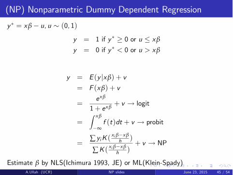
(NP) Nonparametric Dummy Dependent Regression

y ∗ = xb− u, u ∼ (0, 1)

y = 1 if y ∗ ≥ 0 or u ≤ xb

y = 0 if y ∗ < 0 or u > xb

y = E (y |xb) + v

= F (xb) + v

=exb

1+ exb+ v ! logit

=Z xb

−•f (t)dt + v ! probit

=Â yiK (

xi b−xbh )

ÂK ( xi b−xbh )

+ v ! NP

Estimate b by NLS(Ichimura 1993, JE) or ML(Klein-Spady)A.Ullah (UCR) NP slides June 23, 2015 45 / 54

Nonparametric Dummy Dependent Regression

Klein-Spady (1993, Econometrica):log L = Â[F (xi b)yi + (1− yi ) log(1− F (xi b))]

Manski’s Score: Â[I (xi b > ei )yi + (1− yi )(1− I (xi b ≤ ei ))]

Horowitz: Replace I (xi b > ei ) by K (xi bh )


Goodness of Fit

Parametric Regression R2

Yt = Xtq + Ut t = 1, . . . , nmin

qÂ (Yt − Xtq) , q = (X 0X )−1X 0Y

Yt = Xt q + Ut= Yt + Ut

Yt − Y = Yt − Y + UtÂ (Yt − Y )

2= Â

(Yt − Y

)2+Â U2t

ANOVA Decomposition

TSS = ESS + RSS

R2 =ESSTSS

= 1−RSSTSS

Normal Equations

Â Ut = 0, Â UtXt = 0


Nonparametric Regression R2

Nonparametric Regression Estimation

Yt = m (Xt ) + Ut' m (x) + (Xt − x)0 b (x) + Ut= X 0tx d (x) + Ut

where Xtx =[1 (Xt − x)0

]0, d (x) =

[m (x) b0 (x)

]0, Xt is p × 1.


Nonparametric Regression R2 (Local)

Yt = X 0tx d (x) + Ut= Ytx + Ut

Yt − Y = Ytx − Y + Ut(Yt − Y )

2=

(Ytx − Y

)2+ U2t + 2

(Ytx − Y

)Ut

Â (Yt − Y )2 Kh (Xt − x) = Â

(Ytx − Y

)2Kh (Xt − x) +Â U2t Kh (Xt − x)

Local ANOVATSS (x) = ESS (x) + RSS (x)

Normal Equations

Â UtKh (Xt − x) = 0, Â Ut (Xt − x)Kh (Xt − x) = 0

R2 (x) =ESS (x)TSS (x)


Nonparametric Regression R2 (Global)

TSS (x) = ESS (x) + RSS (x)

Â (Yt − Y )2 Kh (Xt − x) = Â

(Ytx − Y

)2Kh (Xt − x) +Â U2t Kh (Xt − x)

[Ytx = X 0tx d (x) = X 0tx(X 0xWxXx

)−1 X 0xWxY ]ZTSS (x) dx =

ZESS (x) dx +

ZRSS (x) dx

Global ANOVA

TSS = ESS + RSS

R2 =ESSTSS

= 1−RSSTSS

ESS = Y 0MH∗MY , H∗ =RHxdx , Hx = WxXx (X 0xWxXx )

−1 X 0xWx

M = In − L, where L is Matrix of 1/n.


Goodness of Fit / Model Selection Measures

R2q =ESSqTSS

= 1−RSSqTSS

= 1−Y 0(In −H∗q

)Y

Y 0MY

R2Adj = 1−RSSq/

(n− trH∗q

)

TSS/ (n− 1)AIC = log (RSSq) + 2tr

(H∗q)

/nBIC = log (RSSq) + (logn) tr

(H∗q)

/n


Global R2 (other definition)

y = m (x) + u

V (y) = V (m (x)) + V (u)

V (y) = V [E (y |x)] + E [V (y |x)]R2 = V [m (x)] / V (y)

= 1−E (y −m (x))2

V (y)

R2 = 1−1n Â (yi − m (xi ))

2

1n Â (yi − y)

2

R = R2I[1n Â (yi − y)

2 ≥1n Â (yi − m (xi ))

2]

Uses of R2: Goodness of Fit: Testing based on R2 (LM type Tests)Su, Ullah (2013, ET), Yao and Ullah (2013, JSPI)


Discrete Data / Mixed Data

X : f (x)?X : Continuous

f (x) =1nh

n

Â1K (xi − xh

) =1nh

n

Â1K (xi , x , h)

Discrete

f (x) =1n

n

Â1L (xi , x ,l)

L (xi , x ,l) = 1− l xi = x

=l

c − 1xi 6= x

for xi 2 {0, 1, . . . , c − 1} , 0 ≤ l ≤ c−1c .For l = c−1

c , L (·) = 1/c .For Regression: xi is discrete

yi = m (xi ) + ui

m (x) =Â yi L (xi , x ,l)Â L (xi , x ,l)

! N-W


Discrete Data / Mixed Data

L (xi , x ,l) = 1− l if xi = x and l otherwise.Mixed Data xi =

[xi1, xi2

], xi1: C and xi2: D

K (xi − xh

) = K (xi1 − x1h

)L (xi2, x2,l)


nonparametric econometrics - wise.xmu.edu.cn ullah—method i.pdf · correlations, earning...

Documents