nonlinear tracking of natural mechanical systems for hwil

NONLINEAR TRACKING OF NATURAL MECHANICAL

SYSTEMS FOR HWIL SIMULATION

Except where reference is made to the work of others, the work described in this thesis is my own or was done in collaboration with my advisory committee. This thesis does not

include proprietary or classified information.

_______________________________ Justin N. Martin

Certificate of Approval: _________________________ _________________________ John E. Cochran, Jr. Andrew J. Sinclair, Chair Professor Assistant Professor Aerospace Engineering Aerospace Engineering _________________________ _________________________ David A. Cicci Joe F. Pittman Professor Interim Dean Aerospace Engineering Graduate School



Justin N. Martin

A Thesis

Submitted to

the Graduate Faculty of

Auburn University

in Partial Fulfillment of the

Requirements for the

Degree of

Master of Science

Auburn, Alabama August 4, 2007

iii



Justin N. Martin

Permission is granted to Auburn University to make copies of this thesis at its discretion, upon request of individuals or institutions and at their expense. The author reserves all

publication rights.

______________________________ Signature of Author

______________________________Date of Graduation

iv

THESIS ABSTRACT



Justin N. Martin

Master of Science, August 4, 2007 (B.S. Aero. Eng., West Virginia University, 2003) (B.S., Mech. Eng., West Virginia University, 2003)

123 Typed Pages

Directed by Andrew Sinclair

Auburn University has entered into collaboration with the US Department of

Defense for academic study and development of hardware-in-the-loop simulation

laboratory. One aspect of this collaboration has been research into new concepts for the

control of flight motion tables, a critical component in HWIL simulations.

Commonly used Proportional-Integral-Derivative (PID) controllers can suffer

limitations in applications with nonlinear and multi-input/multi-output systems. To

overcome these limitations, a nonlinear dynamic-inversion controller was developed.

Applying Lagrange’s equations to determine equations of motion, a Lyapunov function

was used to develop a globally asymptotically stable controller.

v

After comparing PID and dynamic-inversion controllers through multiple

commanded motions and adjustments to gain, the dynamic-inversion was more stable and

produces less error. Both controllers are capable of performing real-time applications.

vi

ACKNOWLEDGMENTS

The author would like to thank Scottie Mobley of the Aviation and Missile

Research Development and Engineering Center and Ryan Brindley and Jeffrey Gareri of

Simulation Technologies, Inc. for their continued assistance with HWIL systems.

vii

Style manual or journal used: Modern Language Association Style Manual

Computer software used: Microsoft Office Word 2003 Microsoft Office Excel 2003 Matlab 7.3.0 (R2006b) UGS Solid Edge V19

viii

TABLE OF CONTENTS

LIST OF TABLES.............................................................................................................. x

LIST OF FIGURES ........................................................................................................... xi

I. INTRODUCTION..........................................................................................................1

II. FLIGHT MOTION TABLES........................................................................................4

III. PID CONTROLLERS .................................................................................................7

Proportional Term....................................................................................................9

Integral Term .........................................................................................................10

Derivative Term.....................................................................................................11

IV. DYNAMIC-INVERSION CONTROLLERS............................................................12

V. MODEL AND CONTROLLER DEVELOPMENT...................................................15

Development of Equations of Motion....................................................................15

PID Program Structure...........................................................................................24

Derivation of Dynamic-inversion Controller.........................................................35

Dynamic-inversion Program Structure ..................................................................38

VI. MODEL SIMULATIONS AND ANALYSIS...........................................................49

General Experimental Set-up.................................................................................49

Commanded Variables and Descriptions of Functions..........................................49

Gain Selections ......................................................................................................52

Model Simulations.................................................................................................53

ix

VII. COMPARISON OF PID AND DYNAMIC-INVERSION CONTROLLERS........69

Comparison of Controls for Each Input.................................................................69

Error Analysis for each Input.................................................................................77

Runtime Analysis for each Input ...........................................................................87

VIII. CONCLUSIONS.....................................................................................................92

BIBLIOGRAPHY..............................................................................................................94

APPENDICES ...................................................................................................................96

Appendix A: Complete Derivation of Equations of Motion.................................97

Appendix B: Complete Derivation of Dynamic-inversion Controller................103

Appendix C: PID and Dynamic-inversion Controller Program..........................105

x

LIST OF TABLES

Table 1.

Table 2.

Table 3.

Table 4.

Table 5.

Performance Specifications .........................................................................6

Trends due to Change in Gains....................................................................8

Moments of Inertia for 3-Gimbaled System ..............................................23

Total Error Comparison of PID and DI controllers ...................................85

Analysis of Runtimes.................................................................................89

xi

LIST OF FIGURES

Figure 1a.

Figure 1b

Figure 2a,b

Figure 3

Figure 4

Figure 5

Figure 6a,b

Figure 7a,b

Figure 8a,b

Figure 9

Figure 10

Figure 11

Figure 12a

Figure 12b

Figure 12c

Figure 12d

Figure 13a

Figure 13b

Figure 13c

Layout of HWIL Laboratory ....................................................................2

ECSEL Laboratory in Point Mugu, CA ...................................................2

Three Axis Flight Motion Table ...............................................................6

Block Diagram of a PID Program.............................................................9

Block Diagram of a Dynamic-inversion Program ..................................13

Inertial CS aligned wit Component #1 CS..............................................16

Component #1 CS aligned with the Inertial CS......................................17

Component #2 CS aligned with the Component #1 CS..........................17

Component #3 CS aligned with the Component #2 CS..........................18

Gimbaled System set to Zero Deflections ..............................................19

PID Program Structure............................................................................25

Dynamic-inversion Program Structure ...................................................39

PID Model for Constant Control and KP = 200, KD = 50 .......................55

DI Model for Constant Control and KP = 200, KD = 50..........................56

PID Model for Constant Control and KP = 400, KD = 100 .....................57

DI Model for Constant Control and KP = 400, KD = 100........................58

PID Model for Step Control and KP = 200, KD = 50 ..............................60

DI Model for Step Control and KP = 200, KD = 50.................................61

PID Model for Step Control and KP = 400, KD = 100 ............................62

xii

Figure 13d

Figure 14a

Figure 14b

Figure 14c

Figure 14d

Figure 15a

Figure 15b

Figure 16a

Figure 16b

Figure 17a

Figure 17b

Figure 18a

Figure 18b

Figure 18c

Figure 19a

Figure 19b

Figure 19c

Figure 20a

Figure 20b

Figure 21a

Figure 21b

DI Model for Step Control and KP = 400, KD = 100...............................63

PID Model for Sinusoidal Control and KP = 200, KD = 50.....................65

DI Model for Sinusoidal Control and KP = 200, KD = 50.......................66

PID Model for Sinusoidal Control and KP = 400, KD = 100...................67

DI Model for Sinusoidal Control and KP = 400, KD = 100.....................68

Control for Constant Command and KP = 200, KD = 50.........................71

Control for Constant Command and KP = 400, KD = 100.......................72

Control for Step Command and KP = 200, KD = 50................................73

Control for Step Command and KP = 400, KD = 100..............................74

Control for Sinusoidal Command and KP = 200, KD = 50......................75

Control for Sinusoidal Command and KP = 400, KD = 100....................76

Error for Constant Command and KP = 200, KD = 50 ............................78

Error for Step Command and KP = 200, KD = 50 ...................................79

Error for Sinusoidal Command and KP = 200, KD = 50..........................80

Error for Constant Command and KP = 400, KD = 100 ..........................82

Error for Step Command and KP = 400, KD = 100 .................................83

Error for Sinusoidal Command and KP = 400, KD = 100........................84

Error Comparison in PID and DI with KP = 200, KD = 50 .....................86

Error Comparison in PID and DI with KP = 400, KD = 100 ...................87

Runtime Comparison in PID and DI with KP = 200, KD = 50 ................90

Runtime Comparison in PID and DI with KP = 400, KD = 100 ..............90

1

I. INTRODUCTION

Prior to Hardware-in-the-Loop (HWIL) simulations, analyses of missile seeker head

performance were conducted by live-fire tested at firing ranges. Missiles, with the seeker

heads already installed, were sold in batches. To demonstrate acceptable performance, a

certain percentage from each batch was field tested. Not only was this risky with the

entire sale depending on a small, random potion of the batch, but it was also expensive

with guaranteed losses of the tested missiles.

HWIL systems simplify this process of testing seeker heads. Rather than needing an

entire range to fire a missile, HWIL systems use a flight motion table and scene

generation to simulate the flight of a seeker head on a missile. The seeker head is placed

in the gimbaled flight motion table while the simulated target is located at a stationary

point in front of the flight table. Using the scene generator and synthetic lines of sight,

the seeker simulates the tracking of a target.

Figure 1a (reproduced from Reference [High Performance]) and Figure 1b (reproduced

from Reference [Hardware]) demonstrate the basic layout of a HWIL laboratory. Figure

1a displays the components and connections for an HWIL simulation, while Figure 1b is

2

a photograph of the Electronic Combat Simulation and Evaluation Laboratory (ECSEL)

located in Point Mugu, CA.

Figure 1a: Layout of HWIL Laboratory

Figure 1b: ECSEL Laboratory in Point Mugu, CA

3

In the summer of 2006, Auburn University, in collaboration with Simulation

Technologies, Inc. and the US Department of Defense, began a program to receive,

install and test a flight table for a HWIL system. One of the goals of Auburn University

is to study the design and implementation of controllers to guide the gimbaled system.

The following paper presents the design and testing of a nonlinear dynamic-inversion

controller with comparison to a Proportional-Integral-Derivative (PID) controller.

4

II. FLIGHT MOTION TABLES

Flight motion tables consist of multiple gimbaled joints whose motion is generated by

hydraulic or electric actuators. The goal of using a flight table in a HWIL simulation is to

reproduce some aspect of the rotational motion of the flight hardware. They are designed

to accurately and precisely direct the motion of a missile seeker head towards a simulated

target in order to replicate an engagement of that target in an actual flight. However,

these tables are not limited in use to missile simulations. Three main functions this table

can serve are:

1) simulating missile seeker head motions for HWIL systems

2) development and testing of guidance and navigational apparatuses

3) testing the stability and motion of satellite systems (Carter 425)

The development of more highly maneuverable missiles, tables and seeker heads adjust

to meet the demands of HWIL simulations. This has led to tables capable of higher

angular accelerations and angular velocities for dictating faster responding (Carter 426).

The actuators being incorporated into these flight tables are required to generate enough

torque to accelerate 50-100 lb. gimbals at rates of 50,000 deg/s2. These requirements can

dictate choices in the materials used to reduce vibration and deformation and also the

types of actuators used to generate the needed torques (Carter 427).

5

Unfortunately, no matter how well the flight table and gimbaled arrangements are

constructed, there will still remain some space between all bearings and connections.

Seeing as how the control in each mode creates an oscillatory damping function until the

error is nearly eliminated, the control will constantly be demanding reversal of torques.

This reversing may lead to problems with pieces impacting each other, vibrations, and

noise (Collins 579). Granted these are not short term catastrophic problems, but it may

lead to wear and tear on the flight table.

Along with the physical design of gimbaled joints and actuators, it is up to the engineer to

determine a controller that will allow motion tracking with as little error as possible.

Errors in the table motion refer to orientation errors: when the system's gimbaled angles

do not exactly match the commanded values.

Major manufacturers of flight motion tables for HWIL laboratories include Acutronic

USA, Inc. and Ideal Aerosmith. They produce tables that can be used in a pitch-yaw-roll

simulation which greatly reduces the cost of developing seeker heads. The basic model

of the table studied in this work is shown in Figures 2a and 2b below and is similar to the

Carco Series S-450R-3 Simulator produced by Acutronic (Three). Some representative

specifications of the flight table are shown in Table 1.

6

Figures 2a-b: Three Axis Flight Motion Table

(a) (b)

Table 1: Performance Specifications

Component and Axis Rotation Performance Spec.

Type of Motion Component #1: Pitch

Component #2: Yaw

Component #3: Roll

Angular Freedom

- +/- 50 deg +/- 50 deg +/- 50 deg

Positioning Accuracy

- 0.002 deg 0.002 deg 0.002 deg

Continuous +/- 200 deg/sec

+/- 200 deg/sec

+/- 1800 deg/sec

Rate Range Non-

Continuous +/- 200 deg/sec

+/- 200 deg/sec

+/- 200 deg/sec

Continuous 20,000

deg/sec2 20,000

deg/sec2 18,000

deg/sec2 Acceleration, w/ load Non-

Continuous 20,000

deg/sec2 20,000

deg/sec2 20,000

deg/sec2

7

III. PID CONTROLLERS

In nearly all mechanically operated systems in the industrial world, controllers are used.

These controller algorithms need to be designed in order meet performance requirements

while also maintaining a reasonable amount of simplicity (Gutirrez). Proportional-

integral-derivative (PID) controllers are widely used to satisfy these conditions. PID or

some forms of the algorithm are currently being used in approximately 95% of control

loops found in modern industries (Astrom 216). The versatility of the PID-control

approach is one reason PID controllers are so prevalent in modern industries.

The three terms of a PID controller (proportional, integral and derivative) all serve a

specific purpose in the control algorithm. As shown in the paragraphs to come, each part

determines how the system will behave. A quick overview will show that the

proportional term allows the controller motion to converge to the desired response but

does not eliminate the steady state error. The integral term will eliminate the steady error

but can degrade the transient response. The derivative term will increase the stability of

the system (PID-Tutorial). Figure 3 below is a block diagram demonstrating the basic

outline of a PID algorithm. The controller signal, u, for a single-input, single-output

(SISO) is:

8

t

KtKK DIP d

dd

eeeu ++= ∫ (1)

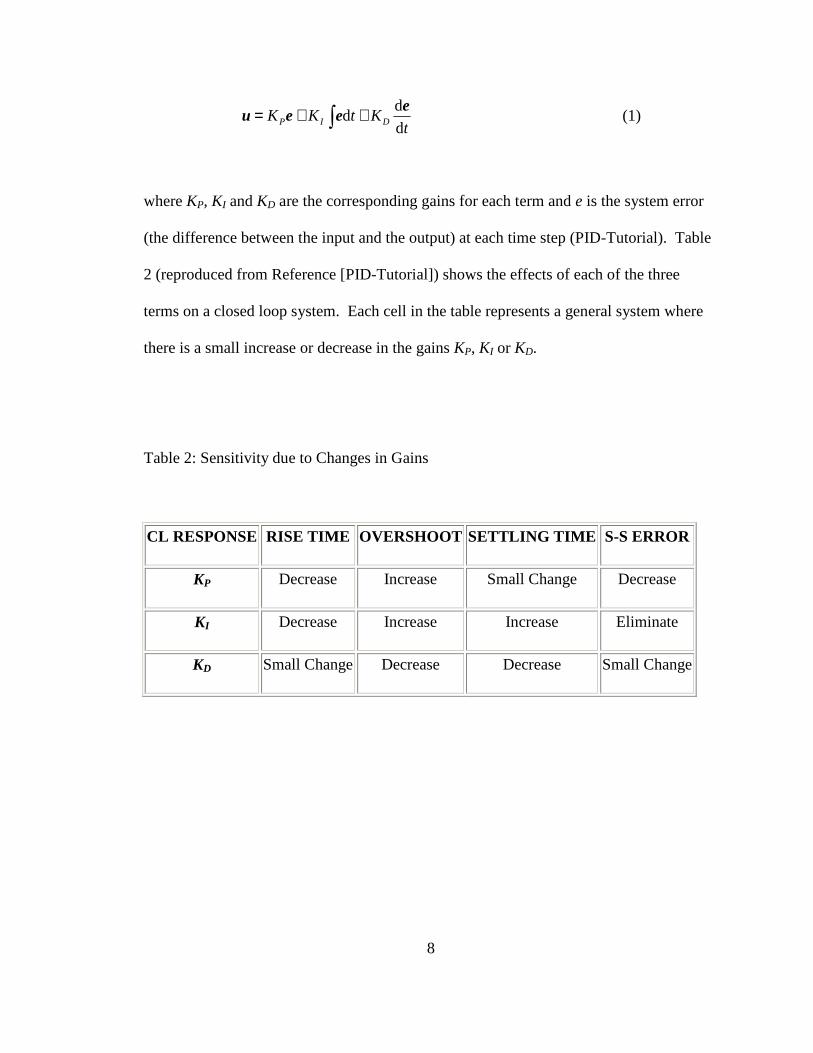
where KP, KI and KD are the corresponding gains for each term and e is the system error

(the difference between the input and the output) at each time step (PID-Tutorial). Table

2 (reproduced from Reference [PID-Tutorial]) shows the effects of each of the three

terms on a closed loop system. Each cell in the table represents a general system where

there is a small increase or decrease in the gains KP, KI or KD.

Table 2: Sensitivity due to Changes in Gains

CL RESPONSE RISE TIME OVERSHOOT SETTLING TIME S-S ERROR

KP Decrease Increase Small Change Decrease

KI Decrease Increase Increase Eliminate

KD Small Change Decrease Decrease Small Change

9

Figure 3: Block Diagram of a PID Program

Integral

Proportional

Derivative

PlantInput Output

+ -

Error

+

++

Proportional Term

As mentioned before, the purpose of the proportional term is to force the system to

respond in the direction of the input. The response is based purely on the error in the

system. If the system is far from convergence, the error is large. Because of the direct

relationship between the proportional control and the error, if the error is large then the

control due to the proportional term is also large and vice versa.

The convergence rate of the system can be greatly affected by the magnitude of KP. By

increasing the value of the proportional gain, the rise time (time it takes to approach the

commanded value) decreased. However, one detail to note is the overshoot (the amount

the gimbaled motion exceeds the commanded motion). Although it will take the system

10

longer to reach the ideal state, the overshoot is smaller, which can help lead to faster

convergence.

The proportional term allows for a brisk adjustment in the controlled variable. However,

it does not provide “zero offset” even though it significantly reduces the error in the

system. The term’s primary purpose is to quicken the response (Marlin 270).

Integral Term

The primary purpose of the integral term is to eliminate or reduce the steady state error,

the error between the input and output of the system as the time approaches infinity. As

shown in Equation 1, the integral term is the area under the curve in an error vs. time

graph. An increase in the transient error is one flaw to the integral term. With an

increase in the integral gain, KI, the rise time decreases. However, increases in overshoot

and settling time (time taken for the system to converge to the commanded value) will

occur. The integral term can help achieve zero offset in the system response to a step

input; unfortunately, it may sometimes cause instability due to its poor dynamic

performance (Marlin 271).

11

Derivative Term

The derivative term is the final piece in the PID controller for creating a stable system.

The derivative term is proportional to the time rate of change in the error. The derivative

term requires “lead”, that is, information about future values of the error, allowing the

controller to react faster to any changes (Gutirrez). This prediction allows the controller

to converge quickly, while increasing stability without the transient error.

By increasing the derivative gain, KD, the damping in the system can be increased.

Greater damping will result in a more rigid system that is slower in convergence. A

negative aspect of this term is that it may require numeric differentiation that can amplify

high frequency noise in the system (Marlin 274).

12

IV. DYNAMIC-INVERSION CONTROLLERS

As discussed in the previous section, PID controllers are not only simple in structure, but

solve a wide range of control cases with suitable results. In order to achieve good

performance with the PID, the tuning of the parameters and the employment of a

functional such as anti-windup and derivative filtering are vital (Visioli). There are also a

few limitations to a PID controller. With a PID, it can be difficult to prove stability for

nonlinear systems (such as a multi-gimbaled system on a flight table). Also, the

implementation of a PID is less clear for multi-input, multi-output (MIMO) systems. An

alternative control structure that may overcome these limitations is dynamic-inversion

control.

According to Looye and Joos, “dynamic-inversion is a straight forward methodology for

designing multi-variable control laws for nonlinear systems (1).” Dynamic-inversion

methods are commonly used in aerospace applications. One such example is the

development of a controller to operate in nonlinear flight schemes such as post-stall

applications (Looye 1). In terms of a flight table, a dynamic-inversion controller is

motivated by the multiple gimbals whose motions affect neighboring gimbals (this is

shown explicitly in the derivation of the equations of motion found in Appendix A).

13

The defining trait of a dynamic-inversion controller is the use of a dynamic model (i.e.

equations of motion) to compute the inputs necessary to generate the desired output.

Hence, the name refers to the inversion of the dynamic model from the form typically

used in solving for system motion. It is noteworthy that a model of the system is built

into the controller, which is not the case in PID control.

A dynamic-inversion controller consists of both feedback and feed-forward sections, as

shown in Figure 4. An inner-loop, structured as a closed loop, applies an inverse in

dynamics in order to negate the nonlinearities in the system (Plett 360). This closed-loop

system is simplified into a set of integrators to be used in the feed-forward section (Looye

1). The feedback section is the outer portion in this arrangement. The feedback loop

contains a standard linear controller, such as a PID controller, in order to minimize

“mismatches” and disturbances in the model created by the nonlinearities (Plett 360).

Figure 4: Block Diagram of a Dynamic-inversion Program

Desired Trajectory

Inverse Model

PD Controller

Plant+

Torque

Output++

-

14

One key to the dynamic-inversion controller is the dynamic model located in the

nonlinear feedback block. The dynamic model is a model of the input-output relationship

for the system to be controlled. Plett suggests allowing the dynamic reference model is a

delayed version of the actual model of the system (364). This would allow the controller

to adjust a priori to a delayed inverse of the system dynamics (Plett 360).

There are some problems to consider when introducing a dynamic-inversion controller

into a system. Looye and Joos state that dynamic-inversion tends to lead to poor

robustness (1). Because the system model is built into the controllers, it is sensitive to

errors in this model. The authors believe the uncertainties can be counteracted by

attempting to increase the robustness of the system within the linear loop (Looye 1).

Other problems created by the dynamic-inversion include the requirement that an inverse

exists (non-singular) and the system typically needs a priori information that may need to

be more precise than that available. Dynamic-inversion techniques, such as adaptive

inverse control, can be applied to the arrangement (Plett 360).

15

V. MODEL AND CONTROLLER DEVELOPMENT

Development of Equations of Motion

To develop controller designs through numerical simulation, a model of the flight-table

motion is required. A specific model is developed in this section in the form of equations

of motion for a flight motion table. Key terms in these equations of motion include the

mass matrix and the Coriolis vector.

The equations of motion for the flight table derived here are based on several

assumptions:

(1) All rotations of coordinate axes are about a single, inertial point.

(2) Piece #1 and #3 are balanced and symmetric, therefore, the moments of

inertia are centered about each component’s symmetrical center of

geometry.

(3) Each component of the system analyzed is a rigid, non-flexible body.

(4) Friction and other applied forces in joints are negligible.

Describing the system kinematics begins with establishing an inertial coordinate system

(CS) ( )ZYX ,, and a separate, body-fixed coordinate system for each individual

16

component studied( )3,2,1for ,,, =izyx iii . All inertial coordinates originate about the

point of all rotations. The coordinate systems are shown in Figures 5 through 8. The

figures of all the components and their set up were designed in Solid Edge. The pieces

are also to scale with the flight table currently located at Auburn University. The

coordinate systems in Figures 6 through 8 are all body-fixed; therefore they are attached

to and rotate with the specific component.

Figure 5: Inertial CS aligned with Component #1 CS with the +Y-axis into the surface

X, x1

Z, z1

17

Figures 6a and 6b: Component #1 CS aligned with the Inertial CS

A positive rotation occurs in the +y1 direction

Figures 7a and 7b: Component #2 CS aligned with the Component #1 CS

A positive rotation occurs in the +z2 direction

Y, y1

Z, z1

Z, z1

X, x1

z1 z2

y1, y2 y1, y2

x1 x2

18

Figures 8a and 8b: Component #3 CS aligned with the Component #2 CS

A positive rotation occurs in the +x3 direction

The entire apparatus with all angles in the { } 3,2,1,, zyx axes set to zero radians is shown in

Figure 9. Note that in the actual experiment, this may not be the starting position of the

components. This is only the reference position used in the equations of motion.

z2, z3 z2, z3

y2 y3

x2 x3

19

Figure 9: Gimbaled System set to Zero Deflections

To specify the orientations of the four coordinate systems, the rotation matrices were

developed. A rotation matrix, in the case of a 3-dimensional system, is a 3x3 matrix that

transforms the unit vector of one coordinate system into a corresponding vector in

another coordinate system. In this case, the rotations are about one of the three axes.

Equation 2a demonstrates the transformation from the coordinate system of component

Y

X

Z

20

#1 to the inertial coordinate system. Note that the rotation occurs about the J (also 1̂j )

axis, which is why a “1” is the multiplying factor in the J row.

−=

1

1

1

11

11

ˆ

ˆ

ˆ

cos0sin

010

sin0cos

k

j

i

K

J

I

θθ

θθ (2a)

Equations 2b and 2c are the transformation matrices for converting the coordinate system

of component #2 to component #1 and the coordinate system of component #3 to

component #2, respectively. In the #2 to #1 transformation, the rotation occurs about the

1̂k (also 2k̂ ) axis. The rotation in the #3 to #2 transformation is about the 2̂i (also 3̂i ) axis.

−=

2

2

2

22

22

1

1

1

ˆ

ˆ

ˆ

100

0cossin

0sincos

ˆ

ˆ

ˆ

k

j

i

k

j

i

θθθθ

(2b)

−=

3

3

3

33

33

2

2

2

ˆ

ˆ

ˆ

cossin0

sincos0

001

ˆ

ˆ

ˆ

k

j

i

k

j

i

θθθθ (2c)

Angular velocities of the coordinate systems can be obtained by inspection. A listing of

the transformed angular velocities can be found in Appendix A.

21

The next step in deriving the equations of motion is to determine the energy in the

rotational system. In his treatise the Mécanique analytique, Lagrange demonstrated laws

of virtual work, which could be applied to the mechanics of both solids and fluids

(Joseph). Rather than follow the work of D’Alembert and Euler by tracking the complete

motion of a particle, he showed that “if we determine its configuration by a sufficient

number of variables whose number is the same as that of the degrees of freedom

possessed by the system, then the kinetic and potential energies of the system can be

expressed in terms of those variables, and the differential equations of motion thence

deduced by simple differentiation (Joseph).” The form of this equation is:

fqqq

=∂∂+

∂∂−

∂∂ VTT

t &d

d (3)

where [ ]T321 θθθ=q and [ ]T321 θθθ &&&& =q are the generalized coordinates and

generalized velocities, T is the kinetic energy of the system defined as the addition of the

rotational kinetic energy of each component, V is the total potential energy, and f is the

generalized external forces on the system. The energies are shown in Equation 4a-b as:

22

( )( )2cos1cossin θδβ −+= LamgV

where ( )

1

1

2

2

1

4

cos12

#2component in offset CG of distance

#2component of mass

θπδ

θπβ

δ

−=

−=

−=

==

La

L

m

(4a)

∑=

=3

12

1

ii

TiT ωIω i (4b)

For component #2, estimations were made for the distance of the center of gravity offset.

In Equation 4b, I indicates the inertia of each body relative to the fixed center of rotation

for the system. By substituting Equation 4 into Equation 3, one can obtain equations of

motion that allow for the development of the mass matrix and the nonlinear Coriolis

vector terms. The complete organization of these matrices and vectors can be found in

Appendix A.

A unique, assumed characteristic of the flight motion table system considered here is that

all parts of the system rotate about a single point. Also, it should be noted that

component #3 is merely a hollowed out cylinder that can be rotated about its longitudinal

axis. Therefore, it can be assumed that I3y and I3z are equivalent. (The actual code used

in numerical simulation is written for the possible case of zy II 33 ≠ for future

experiments). Equations 5 and 6 are the resultant mass matrix and nonlinear Coriolis

23

vector for the assumption of zy II 33 = . The moments of inertia and mass elements were

calculated based on the geometry of the modeled part. The pieces were modeled as

prisms, assumed to be solid casts. Table 3 is a representation of the moments of inertia

for each component.

Table 3: Moments of Inertia for 3-Gimbaled System

Component and Axis Rotation Body

Axis of

Rotation

Component #1:

Pitch (234.9 kg)

Component #2:

Yaw (202.2 kg)

Component #3:

Roll (152.8 kg)

x 57.6 kg-m2 11.9 kg-m2 2.8 kg-m2

y 20.4 kg-m2 10.7 kg-m2 6.8 kg-m2

z 37.8 kg-m2 9.9 kg-m2 6.8 kg-m2

The resulting equations of motion have the form .fhqM =+&& The terms qM && and h have

the following form when zy II 33 = .

( )( ) ( )

+++++

=

3

2

1

323

32

2332

3222

321

0sin

00

sin0cossin

θθθ

θ

θθθ

&&

&&

&&

&&

xx

yz

xyyxxy

II

II

IIIIII

qqM ,

(5)

24

( )

( ){ }( ){ }

∂∂++−+−−

∂∂++−+−

=

2321

23323322121

13323322122

cos

sincos

sin2cos

,

θθθθ

θθθθθ

θθθθθθ

x

xyxyx

xyxyx

I

VIIIII

VIIIII

&&

&&&

&&&

&qqh (6)

The generalized forces of the system are the three control torques exerted by the

hydraulic/electric actuators of the flight table.

ΓΓΓ

=

3

2

1

f (7)

In operation, the torques are the control variables used to force the system motion to track

the commanded motion.

PID Program Structure

The block diagram shown in Figure 10 demonstrates the structure of the Proportional-

Integral-Derivative program. The following is an explanation of each block in the figure.

The explanation includes the parameters involved, the objective of the structure and the

output from the block.

25

Figure 10: PID Program Structure

4. Update TimeStep

PID

5. Call RK44Function(deriv_con)

6. CalculateAngle, AngularRate Derivsand Integrals

7. Update (9x1)State Vector

8. Call Com. Anglesand Rates Func.(commanded_values)

9. ChooseCommandedAngle Types

10. Call ControlFunction(control_develop)

11. DetermineErrors andControl

1. InitializeVariables

See Block Diagram on Dynamic Inversion Controllers

2. Choose Controller

3. Create StateMatrix

Is RuntimeComplete?

Stop

DI

x, f

k (1-4)

i, t(i+1)

Commands

x

f

Yes

No

26

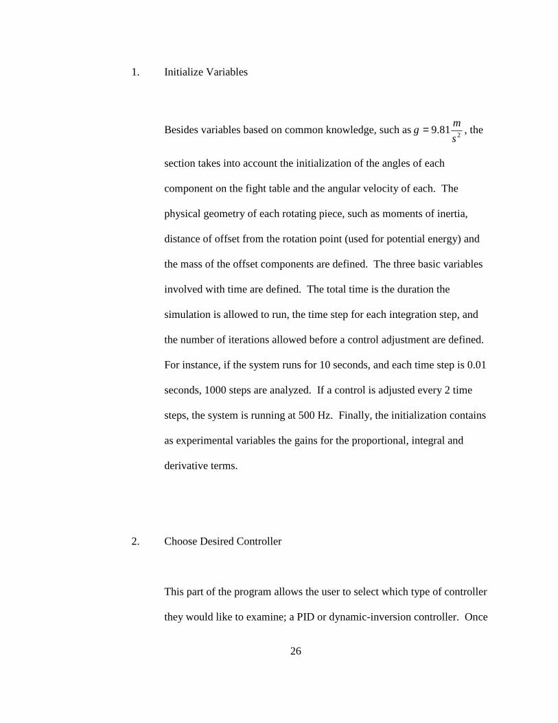
1. Initialize Variables

Besides variables based on common knowledge, such as2

81.9s

mg = , the

section takes into account the initialization of the angles of each

component on the fight table and the angular velocity of each. The

physical geometry of each rotating piece, such as moments of inertia,

distance of offset from the rotation point (used for potential energy) and

the mass of the offset components are defined. The three basic variables

involved with time are defined. The total time is the duration the

simulation is allowed to run, the time step for each integration step, and

the number of iterations allowed before a control adjustment are defined.

For instance, if the system runs for 10 seconds, and each time step is 0.01

seconds, 1000 steps are analyzed. If a control is adjusted every 2 time

steps, the system is running at 500 Hz. Finally, the initialization contains

as experimental variables the gains for the proportional, integral and

derivative terms.

2. Choose Desired Controller

This part of the program allows the user to select which type of controller

they would like to examine; a PID or dynamic-inversion controller. Once

27

the user selects a controller, all the characteristics of that controller are

applied for the remainder of the program. The controller not chosen is

negated for the remainder of the runtime. In this chapter, the PID

controller was selected.

3. Create State Vector

The state vector groups together all the components of the simulation that

will be integrated across time. In the case of the PID controller, the state

vector is a (9 x 1) vector consisting of angular positions for the 3 rotating

components, the three angular rates associated with those components and

the three errors associated with the integral gain in the controller itself.

Grouping all nine components together assures that each cell is updated

simultaneously with the other eight cells.

4. Update the System Time

The arrangement in question is a discrete time system. Therefore, the

values at a specific time step are determined and then evaluated at a small

forward step in the system time,.t∆ When the words “updating the system

time” are used, the program is not automatically changing all the times

28

associated with calculated variables to some new time, ,tt ∆+ but it’s

storing the old and new variables which can then be used for comparison

and error calculations.

5. Call Proportional Integral Derivative RK-44 Function (derive_con)

The PID program was written to take small time steps, integrate them

across those time steps and update the state vector consisting of angles,

angular rates, and integral error, all using a fourth-order Runge-Kutta

integration method. The RK-44 uses the beginning, middle, and end point

of each time step in order to calculate an average time rate of change of

each parameter over that discrete time. The following equations represent

the RK-44 for a second-order system:

( )( )( )[ ]

( )

( )

( )( )[ ]tt

tt

tt

tt

ft

ft

ft

ft

f

ukqqxk

ukqqxk

ukqqxk

uqqxk

qqq

,,

,2

1,

,2

1,

,,

,

34

23

12

1

+∆=

+∆=

+∆=

∆==

&

&

&

&

&&&

The k-terms sent back into the “deriv_con” function, which represents the

RK-44, are (9 x 1) vectors as well. Each cell in the vector corresponds to

29

its respective angle, angular rate or integral error which will be used to

update the state vector, as shown in section 7.

6. Calculate Angle, Angular Rate Derivatives, and Error Integral

The function, “deriv_con”, serves as the integration section of the RK-44.

With the inputs of each portion of the time step, as shown in part 5, the

function calculates the k and z (integral) terms. The k terms are also

referred to as the θ& and θ&& terms. The equations of motion (derived in the

upcoming sections and Appendix A):

( ) ( ) fqqhqqM =+ &&& , (8)

Provide the second time derivatives of the Euler angles.

( ) ( )( )qqhfqMqq

&&&&

,d

d 1 −== −

t (9)

Although the mass matrix, M, is diagonally dominant and invertible, the

“\” function was used in Matlab. This applies a Gaussian Elimination

method for finding a matrix equation of the form bAx = , where A is (nxn)

and x and b are (nx1). The integral for each portion of the time step is also

30

calculated by taking difference between the commanded angles and the

actual angles. The returned vector is a (9 x 1) vector in the form:

( ) ( ) ( )[ ]Txxx 31313141 zqqk &&&&=−

Note that all the components are the derivatives, or slope, of its integrated

part. This vector is returned to the main program in order to update the

state vector.

7. Update State Vector

Once all the derivatives of the angles, angular rates and integral errors are

sent back to the main program, the last piece of the 4th Order Runge-Kutta

is applied. This part of the RK-44 updates the angles, angular rates and

error integral across the discrete time step using the equation:

( )( )43211 26

1kkkkxx ++++=+ ii (10)

The updated state matrix will be used for calculating the errors present and

the required controls for the next iteration of the main program.

31

8. Call the Commanded Angles and Rates Function (commanded_values)

This section of the program loop is one of the key factors for designing the

experiment. The commanded angles, angular rates and angular

accelerations are very similar to the simulated path of a target that the

seeker is trying to follow. This portion of the program relays the position,

speed, and the rate of change in speed the gimbals should be achieving.

These commanded angles and rates are calculated in the

“commanded_values” function. The variables sent to this function are the

time step iteration number and the updated time of the system.

9. Determine Control Angle and Rate Types

The simulated motion can take many shapes and forms. The three types of

simulations that are going to be examined are the constant direction and

angular velocity, a constant position and angular velocity followed up with

an impulsive change in position at a given time step, and a constantly

changing (in this case sinusoidal) position and velocity. The constant

position and angular velocity scenario takes a random gimbaled placement

and tracks the motion of the positions of the interceptor and target as they

maneuver to another position over the course of the simulation. The

position and angular velocity with an impulsive change tracks the position

32

as it settles, instantaneously changes to another commanded position, and

tracks the gimbals’ motion for the duration of the simulation time. The

sinusoidal position and velocity applies a commanded sine form of

position, velocity and acceleration that the gimbals must track.

The main program will receive a (9 x 1) vector, represented as:

[ ]Tcomcomcomcommand qqqy &&&=

The three scenarios are further described and demonstrated in the

Commanded Variables and Description of Functions section.

10. Call the Control Function (control_develop)

Now stored in the program is the updated system time, a corresponding

state vector and a commanded position and rate vector. However, as

mentioned before, the values of these two vectors may not agree, creating

some error in the results. To minimize this error, a control is applied to

the necessary gimbals where it is required. This control is determined in

the function “control_develop”. The required inputs for this function are

both the state vector and commanded angles and rates vector. The

33

function will calculate the control required for the next iteration of the

main program.

11. Determine the Three PID Errors and Controls

As discussed in previous chapters, there are three types of errors to

analyze in a PID controller system; the proportional, integral and

derivative. Having a commanded angle and an angular rate relayed to the

function, the position and speed each component should calculated. Also,

after completion of the RK-44 and an update of the variables, an actual set

of angles and angular rates are determined. Unless everything in the

system was 100% perfect, there is bound to be some error in the nonlinear

arrangement. Therefore, it is necessary to find the errors for each section

of the PID controllers. The error used in the proportional controller is

simply the difference between the commanded and actual position of each

component. The integral controller error is represented by the “z” term

found from integrating the difference between the commanded and actual

angle of each component from the beginning to the current time of the

simulation. The error used in the derivative portion of the controller is

difference between the commanded and actual angular velocities of each

component.

34

As discussed before, the basic equation used in the majority of PID

controllers is represented by Equation 1:

t

KtKK DIP d

dd

eeeu ++= ∫

Note that in the previous section, the three errors defined correspond,

respectively, to the errors in the equation. The values of the gains have

already been defined in the initialization of all parameters section. These

gains can be adjusted in order permit the system to more precisely

converge to the commanded angles and angular velocities. The value of

the control, u, a (3 x 1) vector in this case, is then updated and applied

back into Equation 9, until further updated. The control, u, is then relayed

back to the main program.

12. Is Runtime Complete?

No matter how long the system runs, there is always going to be some

oscillation error due to fact that a small time segment is used, rather than a

continuous signal. However, after a certain time, the error in the system is

considered negligible. The runtime value, defined in the initialization

section, is used by the programmer to ensure the program will terminate

35

after a specific simulation time. Once a discrete value of t∆ is added to the

system time, the program checks to see if the termination time has been

achieved. If so, the program terminates. If the time has not been reached,

the program loops back to Section 2, and repeats all the steps leading up to

Section 12.

Derivation of Dynamic-inversion Controller

When deriving the dynamic-inversion controller for a motion flight table, the problem is

classified in the category of tracking controllers for nonlinear natural mechanical

systems. Remember that a natural mechanical system is one where all the terms in the

kinetic energy are quadratic in the generalized velocities, .q&

Because of this property of natural mechanical systems, the kinetic energy of the system

can be written as:

( ) ( ) jiijT qqMT &&&&&

2

1

2

1, == qqMqqq (11)

where T is the kinetic energy and M is the mass matrix. In order to determine the

equations of motion, as required for the dynamics of the flight table, Lagrange’s equation

36

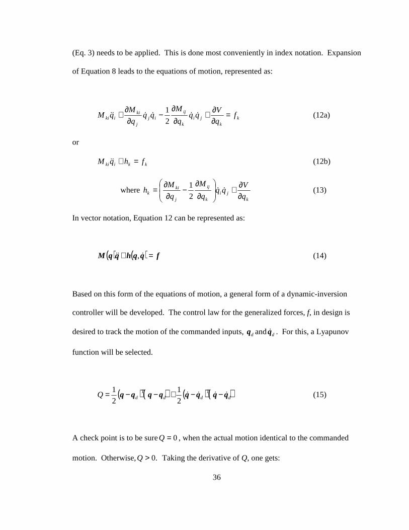
(Eq. 3) needs to be applied. This is done most conveniently in index notation. Expansion

of Equation 8 leads to the equations of motion, represented as:

kk

jik

ijij

j

kiiki f

q

Vqq

q

Mqq

q

MqM =

∂∂+

∂∂

−∂

∂+ &&&&&&

2

1 (12a)

or

kkiki fhqM =+&& (12b)

where k

jik

ij

j

kik q

Vqq

q

M

q

Mh

∂∂+

∂∂

−∂

∂= &&

2

1 (13)

In vector notation, Equation 12 can be represented as:

( ) ( ) fqqhqqM =+ &&& , (14)

Based on this form of the equations of motion, a general form of a dynamic-inversion

controller will be developed. The control law for the generalized forces, f, in design is

desired to track the motion of the commanded inputs, dq and dq& . For this, a Lyapunov

function will be selected.

( ) ( ) ( ) ( )dT

ddT

dQ qqqqqqqq &&&& −−+−−=2

1

2

1 (15)

A check point is to be sure 0=Q , when the actual motion identical to the commanded

motion. Otherwise, .0>Q Taking the derivative of Q, one gets:

37

( ) ( )ddT

dQ qqqqqq −+−−= &&&&&&& (16)

Here, dq&& are the accelerations associated with the commanded motion. The condition of a

global asymptotically stable system can be achieved by choosing:

( )ddd qqqqqq &&&&&& −−=−+− (17)

The commanded motion can be substituted into the equations of motion to definedf , the

generalized forces necessary to produce this motion.

( ) ( )( )ddddd qqhfqMq &&& ,1 −= − (18)

A globally asymptotically stable controller used to track a desired motion for the natural

mechanical system may be found by solving Equation 14 for q&& and substituting along

with Equation 18 back into Equation 17.

( ) ( ) ( ) ( ) ( ) ( )( )( ) ( ) ( )[ ]dd

dddd

qqqqqM

qqhqMqMqq,hfqMqMf -1d

&&

&&

−+−−−+= −

,1

(19)

The performance of this nonlinear controller will be compared with a typical linear PID

controller. A more detailed derivation can be found in Appendix B. From Equation 19,

it can be seen that the feedback terms in this controller are a form of proportional-

38

derivative (PD) control. The PD controller can alleviate unmodeled dynamics and

disturbances (Yan 199). Therefore, in comparison with the PID controller laid out in the

previous section, the dynamic-inversion controller does not require error integral

information. This is, however, a result of the choice of the Lyapunov function. The

dynamic-inversion controller does require knowledge of commanded accelerations (in

order to computedf ), which were not required by the PID controller. In implementation

some means of computing dq&& is necessary.

Dynamic-inversion Program Structure

The block diagram shown in Figure 11 demonstrates the structure of the dynamic-

inversion program. The following is an explanation of each block in the figure. The

explanation includes the parameters involved, the objective of the structure and the

output from the block. Many of these sections are very similar to those in the PID

description, mainly because the dynamic-inversion controller is the only difference in the

system. A positive attribute to this program is the flexibility of examining whichever

controller the user prefers. Therefore, the majority of the steps and processes are

mirrored for each controller.

39

Figure 11: Dynamic-inversion Program Structure

4. Update TimeStep

DI

5. Call RK44Function(deriv_con)

6. CalculateAngle, AngularRate Derivsand Integrals

7. Update (6x1)State Vector

8. Call Com. Anglesand Rates Func.(commanded_values)

9. ChooseCommandedAngle Types

10. Call ControlFunction(control_develop)

11. DetermineErrors andControl

1. InitializeVariables

See Block Diagram on Prop-Int-Deriv Controllers

2. Choose Controller

3. Create StateMatrix

Is RuntimeComplete?

Stop

PID

x, f

k (1-4)

i, t(i+1)

Commands

x

f

Yes

No

12. Components ofActual and Reference Controls

ComponentsAngleVelocity

40

1. Initialize Variables

To compare the PID arrangement to that of the dynamic-inversion in a fair

manner, the same initial variables must be used. Therefore, the moments

of inertia, mass of each component, distance of component offset, initial

positions and angular velocities, and time step variables (including the

frequency of control adjustments) must remain equal to those in the PID

experiment. The only difference lies in the gains used in the dynamic-

inversion. Only proportional and derivative gains are used and their

values will be different following proper tuning to compliment the

arrangement.

2. Choose Desired Controller

As mentioned before, the user has the ability to select which type of

controller they chose to examine; a PID or dynamic-inversion controller.

Once the user selects a controller, all the characteristics of that controller

are applied for the remainder of the program. In this chapter, the

dynamic-inversion controller was selected. Therefore, the PID controller

characteristics and processes are negated for the remainder of the runtime.

41

3. Create the State Vector

The state vector combines all the components that will be integrated

across the simulation time. In the case of the dynamic-inversion

controller, the state vector is a (6 x 1) vector consisting of angular

positions for the three rotating components and the three angular rates

associated with those components: [ ]Tqqx &= . Unlike the PID state

vector, there is no integral error present due to the form of the controller.

The error across this controller is not integrated; therefore, the gain is not

necessary. This set-up assures that all six variables will be updated and

applied simultaneously throughout the simulation.

4. Update the System Time

The process of updating the system time by a discrete time step, ,t∆ serves

the same purpose as the PID controller. This update is merely a process of

storing and comparing the values of the state vector, command vector, and

control vector for any given time step throughout the simulation. It allows

the user to specify which value at a specific instant they would prefer to

examine.

42

5. Call Dynamic-inversion RK-44 Function (deriv_con)

Similar to the PID program, the dynamic-inversion is analyzed over

constant time steps of ,t∆ therefore integration across those discrete times

is necessary. Once again, a fourth-order Runge-Kutta numerical

integration is going to be applied to the system. All equations are going to

be the same, with the exception of the k terms. Before, in the PID

program, each returned value of k contained three angular derivatives,

three angular velocity derivatives, and three error integrations. The error

integrations are not necessary; therefore, the k values are a (6 x 1) vector,

rather than a (9 x 1). The called function, “deriv_con”, is the same

function used for PID controller, only modified to cater to both

controllers.

6. Calculate Angle and Angular Rate Derivatives

The function, “deriv_con”, is the exact same function used for the PID

controller, except in this situation, the calculation of the integral error over

the specific time step is not applied. Both functions serve the purpose of

determining the rate change in the angular velocity, as previously shown

in Equation 9:

43

( ) ( )( )qqhfqMqq

&&&&

,d

d 1 −== −

t

The resulting q& and q&& terms are returned to the main program as a (6 x 1)

vector in the form of:

( ) ( )[ ]Txx 313141 qqk &&&=−

This vector is returned to the main program in order to update the state

vector by completing the RK-44 integration.

7. Update the State Vector

Once all of the angular rates and angular accelerations are returned to the

main program, the last function of the fourth-order Runge-Kutta is

performed. This part of the RK-44 updates the angles and angular

velocities across the discrete time step, ,t∆ using the same equation as that

of the PID controller:

( )( )43211 26

1kkkkxx ++++=+ ii

44

The updated state matrix will be used for calculating the errors in the

commanded and actual angles and the required controls for the next

iteration of the main program.

8. Call the Commanded Angles and Rates Function (commanded_values)

The commanded angles, angular rates, and angular accelerations are the

motion that the controller is trying to track. This portion of the program

relays the position, the speed, and the rate of change in speed the gimbals

should be achieving. For comparison, the commanded values calculated

in this section will be the same as those used in the PID experiments.

These commanded angles and rates are calculated in the

“commanded_values” function. The variables sent to this function are the

time step iteration number and the updated time of the system.

9. Determine Control Angle and Rate Types

Three basic types of simulations were chosen to study the performance of

the dynamic-inversion controller: (1) constant direction and angular

velocity, (2) constant position and angular velocity followed up with an

impulsive change in position at a given time step, and (3) constantly

45

changing (in this case sinusoidal) position and velocity. The same

commanded angles and angular velocities will be used in the PID program

to ensure an accurate comparison in the results of both controllers. The

returned variable is a (9 x 1) vector, represented as:

[ ]Tcomcomcomcommand qqqy &&&=

The three scenarios are further described and demonstrated in the

Commanded Variables and Description of Functions section.

10. Call the Control Function (control_develop)

The variables required to calculate the updated errors and control for the

1+it conditions are now saved into the state vector and command vector.

Assuming the vectors do not agree, whether machine error or an error

caused by a change in the commanded angles and velocity, the

“control_develop” function allows for a correction control to be produced.

The required inputs for this function are both the state vector and

commanded angles and rates vector. The function will calculate the

control required for the next iteration of the main program.

46

11. Call Commanded and Actual Components Function (model_components)

One of the unique characteristics of a dynamic-inversion controller is the

comparison between the actual components of the equations of motion and

some reference components based off commanded values in order to

determine the control applied to the next time interval. The reference

value components consist of the angles, angular rates, mass matrix,

Coriolis terms and control. These terms are calculated in the function,

“model_components” and returned to “control_develop” function for

analysis. Once the terms are returned, they are applied in the control

equation for this particular dynamic-inversion controller which will be

derived in the following section:

( ) ( ) ( ) ( ) ( ) ( )( )( ) ( ) ( )[ ]dd

dddd

qqqqqM

qqhqMqMqq,hfqMqMf -1d

&&

&&

−+−−−+= −

,1

(19)

The first part of the Equation [19] represents the feedback portion of the

controller. The second condition of the equation is a nonlinear feedback

term comparing the difference between the Coriolis terms of the reference

and actual motions. The last term is a PD form of a controller that is a

nonlinear feedback as well.

47

All the terms in Equation 19 are generated in “model_components”, with

the exception of the commanded and actual angles and angular rates. The

inputs for this function are the actual and commanded angles and angular

velocities. Once the new control is calculated, it is returned to the main

program in order to be applied to the next iteration, starting at Section 4.

12. Determine Commanded and Actual Value Components

The function, “model_components”, for the reference portion uses

Equation 5 to determine the mass matrix, Equation 6 to determine the

Coriolis terms, and Equation 8 to determine the reference control. All

these values are in correspondence with the simulated motion of the

system.

The actual value components consist of the angles, angular rates, mass

matrix, and Coriolis terms. These values are determined in a similar

fashion to the reference components, using the same order and equations,

with the exception that the returned variables represent the actual

characteristics of the system. The applied control is not calculated until

the five characteristics of the motion at that particular time step are

returned to the “control_develop” function.

48

13. Is Runtime Complete?

Just like in the PID controller, there is always going to be some sort of

small error in the simulation, where after a certain time, the error in the

system is negligible (if properly designed). Once a discrete value oft∆ is

added to the system time, the program checks to see if the termination

time has been achieved, ceasing to program if it has. If the time has not

been reached, the program loops back to Section 2, and repeats all the

steps leading up to Section 13, only to be tested again.

49

VI. MODEL SIMULATIONS AND ANALYSIS

General Experimental Set-up

The tri-gimbaled system has three basic parameters which need to be considered when

designing an accurate and precise response to a given command. The factors which will

be examined are the type of controller, the type of commanded angles, angular velocities

and angular accelerations, and the gain levels used in the simulation. As discussed in

previous chapters, the controllers analyzed are of type PID and dynamic-inversion, and

the commanded positions and rates are constant, steps and sinusoidal. The experiments

will also examine how the system changes with increases in both the proportional and

derivative gains.

Commanded Variables and Description of Functions

The commanded variables consist of constant variables, alternating variables (a step

function), and a constantly adjusting sinusoidal command.

50

Prior to every simulation, some factors of the gimbals are set. All three gimbals are

initially set to +0.4 radians from their “home” position. This offset will require an initial

maneuver to be performed in order to approach the commanded position. The gimbals

will all start from rest.

The controller must now track one of the following commanded parameters:

1. Constant Commanded Angles and Rates

With all three gimbaled positions set to +0.4, an alternate set of gimbaled

positions is commanded to force the controller to adjust all three controls

simultaneously. The values for these gimbals after the commanded

controls begin are:

[ ][ ][ ]Tcom

Tcom

Tcom

000

000

2.01.01.0

=

=

=

θ

θ

θ

&&

&

2. Constant Commanded Angles and Rates with a Step Function

This commanded function is very similar to the constant commanded

positioning function described in the previous section with one basic

51

difference. The commanded function travels along a constant angle for all

components then impulsively maneuvers to a different angular position.

For the experiments, the positions are:

[ ][ ]Tcom

Tcom

t

t

5.02.02.0:sec105

2.01.01.0:sec50

=→=

=→=

q

q

Because this is a discrete time system and the time step is small, the

angular velocity and angular acceleration expressions remain the same.

3. Consistent Sinusoidal Commanded Path

For this commanded motion, the angles of all three components are all

going to be based off a sinusoidal wave with amplitude of 0.5 radians and

frequency of π21 Hz. Because these angular positions are based on time,

the angular velocities and accelerations can be represented as the first and

second derivative of the position vector.

[ ][ ]

[ ]Tcomcom

Tcomcom

Tcom

tttt

tttt

ttt

sin5.0sin5.0sin5.0d

d

cos5.0cos5.0cos5.0d

d

sin5.0sin5.0sin5.0

2

2

−−−==

==

=

qq

qq

q

&&

&

52

This method of determining the rates is valid as long as the commanded

position of each component is a function of time.

Gain Selections

It is typically assumed that the larger the gain in a system, the less robust (more sensitive

to errors in the dynamic model) the system becomes. However, the experiments

performed are not to find the optimal gains in the simulation; only to deduce the effect

that a change in gains has on each controller.

After numerous trials of various gains, two sets of gains were selected as appropriate for

the experiments. The first set was KP = 200 and KD = 50. This set of gains allows the

motion and response to be more flexible. The second set is a more aggressive set with

the gains set to KP = 400 and KD = 100. For each experiment run with the PID controller,

the KI gain was set equal to the KP gain. The dynamic-inversion controller does not

utilize the integral gain.

These two sets of gains were compared alongside the three commanded motion and the

two different types of controllers, producing twelve sets of results.

53

Model Simulations

Three commanded motion, two sets of controller gains, and two different controllers are

to be examined. Adjusting every parameter to perform a single study in order to find out

the characteristics and effects of that parameter leads to twelve different situations to

consider. This section will break those twelve simulations into three groups of four tests.

Those three groups will be run with the types of commanded motion. Within each group,

the changes in both the gains and controller will be observed through the angular motions

of the gimbals. An analysis of the applied controls, errors, and run times will be

addressed in later sections.

Input 1: Constant Commanded Angles and Rates

The first simulation tested will compare the PID and dynamic-inversion

controllers with a change in gains. These will be conducted with the commanded

angles, angular velocities and angular accelerations held constant throughout a 10

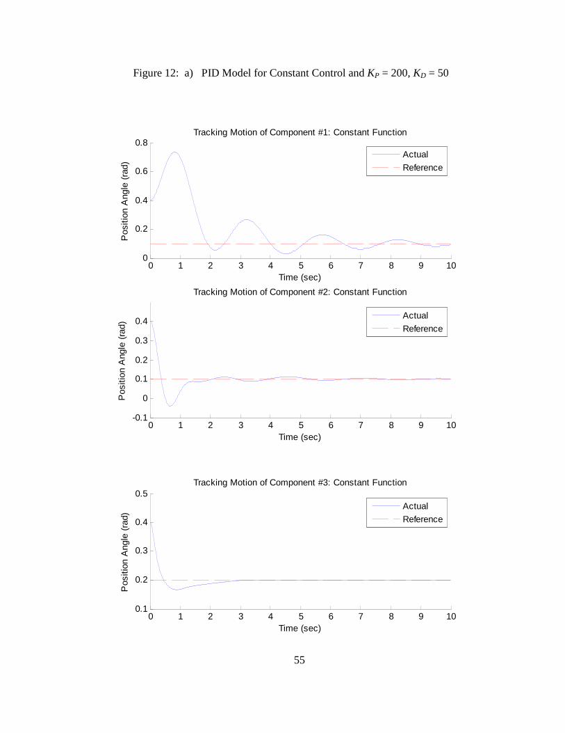
second test period. Figures 12a and 12b represent a PID and dynamic-inversion

controller under the influence of a proportional gain equal to 200 and a derivative

gain equal to 50.

After the initial jump from the +0.4 radian position, all components controlled

through the PID show difficulties in convergence. The pitch component (piece

54

#1) shows the greatest error in convergence. However, the dynamic-inversion

controller seems to converge in nearly every piece before one second has elapsed.

Figures 12c and 12d are for the same situation, except the gains have increased

significantly. Note that the PID system still has convergence problems, but seems

more in control due to the gain increase. The dynamic-inversion does not seem to

have difficulties with the larger gains. The convergence time in the dynamic-

inversion controllers remained about the same. With the larger gains applied, the

PID controller began to respond similarly to the dynamic-inversion controller.

55

Figure 12: a) PID Model for Constant Control and KP = 200, KD = 50

0 1 2 3 4 5 6 7 8 9 100

0.2

0.4

0.6

0.8

Time (sec)

Pos

ition

Ang

le (

rad)

Tracking Motion of Component #1: Constant Function

Actual

Reference

0 1 2 3 4 5 6 7 8 9 10-0.1

0

0.1

0.2

0.3

0.4

Time (sec)

Pos

ition

Ang

le (

rad)


Actual

Reference

0 1 2 3 4 5 6 7 8 9 100.1

0.2

0.3

0.4

0.5

Time (sec)

Pos

ition

Ang

le (

rad)


Actual

Reference

56

Figure 12: b) DI Model for Constant Control and KP = 200, KD = 50

0 1 2 3 4 5 6 7 8 9 100

0.1

0.2

0.3

0.4

0.5

Time (sec)

Pos

ition

Ang

le (

rad)


Actual

Reference

0 1 2 3 4 5 6 7 8 9 100

0.1

0.2

0.3

0.4

0.5

Time (sec)

Pos

ition

Ang

le (

rad)


Actual

Reference

0 1 2 3 4 5 6 7 8 9 100

0.1

0.2

0.3

0.4

0.5

Time (sec)

Pos

ition

Ang

le (

rad)


Actual

Reference

57

Figure 12: c) PID Model for Constant Control and KP = 400, KD = 100

0 1 2 3 4 5 6 7 8 9 100

0.1

0.2

0.3

0.4

0.5

Time (sec)

Pos

ition

Ang

le (

rad)


Actual

Reference

0 1 2 3 4 5 6 7 8 9 100

0.1

0.2

0.3

0.4

0.5

Time (sec)

Pos

ition

Ang

le (

rad)


Actual

Reference

0 1 2 3 4 5 6 7 8 9 100

0.1

0.2

0.3

0.4

0.5

Time (sec)

Pos

ition

Ang

le (

rad)


Actual

Reference

58

Figure 12: d) DI Model for Constant Control and KP = 400, KD = 100

0 1 2 3 4 5 6 7 8 9 100

0.1

0.2

0.3

0.4

0.5

Time (sec)

Pos

ition

Ang

le (

rad)


Actual

Reference

0 1 2 3 4 5 6 7 8 9 100

0.1

0.2

0.3

0.4

0.5

Time (sec)

Pos

ition

Ang

le (

rad)


Actual

Reference

0 1 2 3 4 5 6 7 8 9 100

0.1

0.2

0.3

0.4

0.5

Time (sec)

Pos

ition

Ang

le (

rad)


Actual

Reference

59

Input 2: Constant Commanded Angles and Rates with a Step Function

The procedure of testing for this mode is nearly identical to that of Input 1 with

the exception that a step function was applied at the 5 second mark. However,

from 0 to 5 seconds and 5 to 10 seconds, the commanded angles and rates remain

constant.

Figures 13a and 13b represent a PID and dynamic-inversion controller with a

proportional gain equal to 200 and a derivative gain equal to 50. Figures 13c and

13d represent the same except that more aggressive KP and KD gains of 400 and

100 respectively were applied.

Similar to the previous mode, the dynamic-inversion has quicker reaction and

convergence times than the PID controller. In fact, the PID controller only seems

to be efficient when the gains are high. However, even after the gains are

increased, there is still a significant amount of overshoot in the PID. The

dynamic-inversion controller contains little to no overshoot and dampens out

quickly in both cases.

60

Figure 13: a) PID Model for Step Control and KP = 200, KD = 50

0 1 2 3 4 5 6 7 8 9 100

0.2

0.4

0.6

0.8

Time (sec)

Pos

ition

Ang

le (

rad)

Tracking Motion of Component #1: Step Function

Actual

Reference

0 1 2 3 4 5 6 7 8 9 10

0

0.2

0.4

0.6

0.8

Time (sec)

Pos

ition

Ang

le (

rad)


Actual

Reference

0 1 2 3 4 5 6 7 8 9 100.1

0.2

0.3

0.4

0.5

0.6

0.7

Time (sec)

Pos

ition

Ang

le (

rad)


Actual

Reference

61

Figure 13: b) DI Model for Step Control and KP = 200, KD = 50

0 1 2 3 4 5 6 7 8 9 100

0.1

0.2

0.3

0.4

0.5

Time (sec)

Pos

ition

Ang

le (

rad)


Actual

Reference

0 1 2 3 4 5 6 7 8 9 10-0.1

0

0.1

0.2

0.3

0.4

0.5

Time (sec)

Pos

ition

Ang

le (

rad)


Actual

Reference

0 1 2 3 4 5 6 7 8 9 100.1

0.2

0.3

0.4

0.5

0.6

Time (sec)

Pos

ition

Ang

le (ra

d)


Actual

Reference

62

Figure 13: c) PID Model for KP = 400, KD = 100

0 1 2 3 4 5 6 7 8 9 100

0.1

0.2

0.3

0.4

0.5

Time (sec)

Pos

ition

Ang

le (

rad)


Actual

Reference

0 1 2 3 4 5 6 7 8 9 10-0.1

0

0.1

0.2

0.3

0.4

0.5

Time (sec)

Pos

ition

Ang

le (

rad)


Actual

Reference

0 1 2 3 4 5 6 7 8 9 100.1

0.2

0.3

0.4

0.5

0.6

Time (sec)

Pos

ition

Ang

le (

rad)


Actual

Reference

63

Figure 13: d) DI Model for KP = 400, KD = 100

0 1 2 3 4 5 6 7 8 9 100

0.1

0.2

0.3

0.4

0.5

Time (sec)

Pos

ition

Ang

le (

rad)


Actual

Reference

0 1 2 3 4 5 6 7 8 9 10-0.1

0

0.1

0.2

0.3

0.4

0.5

Time (sec)

Pos

ition

Ang

le (

rad)


Actual

Reference

0 1 2 3 4 5 6 7 8 9 100.1

0.2

0.3

0.4

0.5

0.6

Time (sec)

Pos

ition

Ang

le (

rad)


Actual

Reference

64

Input 3: Sinusoidal Commanded Motion

The following mode is most similar to that of a guided missile simulation in an

HWIL system. The relative motion between the seeker and target is more likely

to be in the form of smooth curves getting sharper as the missile approaches the

target rather than instantaneous steps in position. Therefore, the results from this

mode are probably more relevant to flight motion table simulations. The motion

is a simple sinusoidal wave function which oscillates for a total duration of 10

seconds.

Figures 14a and 14b represent a PID and dynamic-inversion controller with a

proportional gain equal to 200 and a derivative gain equal to 50. Figures 14c and

14d represent the same except that more aggressive KP and KD gains of 400 and

100 respectively were applied.

In this mode, the dynamic-inversion has little to no overshoot in both cases while

still managing to converge to the curve within first second of the simulation.

Contrary to the dynamic-inversion results, the PID controller seemed to struggle

in its convergence on the constantly changing curve, most likely due to the

integral term. Figure 14a shows difficulty in the pitch and yaw, while Figure 14c

shows difficulty converging at the peaks of the sine wave.

65

Figure 14: a) PID Model for Sinusoidal Command and KP = 200, KD = 50

0 1 2 3 4 5 6 7 8 9 10-1

-0.5

0

0.5

1

Time (sec)

Pos

ition

Ang

le (

rad)

Tracking Motion of Component #1: Sinusoidal Function

Actual

Reference

0 1 2 3 4 5 6 7 8 9 10-1

-0.5

0

0.5

1

Time (sec)

Pos

ition

Ang

le (

rad)


Actual

Reference

0 1 2 3 4 5 6 7 8 9 10-1

-0.5

0

0.5

1

Time (sec)

Pos

ition

Ang

le (

rad)


Actual

Reference

66

Figure 14: b) DI Model for Sinusoidal Command and KP = 200, KD = 50

0 1 2 3 4 5 6 7 8 9 10

-0.6

-0.4

-0.2

0

0.2

0.4

0.6

Time (sec)

Pos

ition

Ang

le (

rad)


Actual

Reference

0 1 2 3 4 5 6 7 8 9 10

-0.6

-0.4

-0.2

0

0.2

0.4

0.6

Time (sec)

Pos

ition

Ang

le (

rad)


Actual

Reference

0 1 2 3 4 5 6 7 8 9 10

-0.6

-0.4

-0.2

0

0.2

0.4

0.6

Time (sec)

Pos

ition

Ang

le (

rad)


Actual

Reference

67

Figure 14: c) PID Model for Sinusoidal Command and KP = 400, KD = 100

0 1 2 3 4 5 6 7 8 9 10

-0.6

-0.4

-0.2

0

0.2

0.4

0.6

Time (sec)

Pos

ition

Ang

le (

rad)


Actual

Reference

0 1 2 3 4 5 6 7 8 9 10

-0.6

-0.4

-0.2

0

0.2

0.4

0.6

Time (sec)

Pos

ition

Ang

le (

rad)


Actual

Reference

0 1 2 3 4 5 6 7 8 9 10

-0.6

-0.4

-0.2

0

0.2

0.4

0.6

Time (sec)

Pos

ition

Ang

le (

rad)


Actual

Reference

68

Figure 14: d) DI Model for Sinusoidal Command and KP = 400, KD = 100

0 1 2 3 4 5 6 7 8 9 10

-0.6

-0.4

-0.2

0

0.2

0.4

0.6

Time (sec)

Pos

ition

Ang

le (

rad)


Actual

Reference

0 1 2 3 4 5 6 7 8 9 10

-0.6

-0.4

-0.2

0

0.2

0.4

0.6

Time (sec)

Pos

ition

Ang

le (

rad)


Actual

Reference

0 1 2 3 4 5 6 7 8 9 10

-0.6

-0.4

-0.2

0

0.2

0.4

0.6

Time (sec)

Pos

ition

Ang

le (

rad)


Actual

Reference

69

VII. COMPARISON OF PID AND DYNAMIC-INVERSION CONTROLLERS

In addition to studying the gimbaled-angle histories, other methods can be used to

compare the performance of the PID and dynamic-inversion controllers. As shown in the

previous chapter, the PID controller consistently showed more fluctuation between the

actual and commanded motion. This section describes an investigation of the control

torques and processor time required by both the PID and dynamic-inversion controllers.

Comparison of Controls for each Input

Two factors being considered while looking at the control for each of the twelve systems

are the settling time (how long is the controller required to operate before convergence)

and the maximum control required. These two factors can play a role not only in the

system performance, but also the life span of the flight table.

The controls for all three components, both controllers and all three commanded inputs

are shown in Figures 15-17. A common trend is present in all results shown. Concerning

the PID controller, the reaction is slower and the control is more oscillatory. However,

the controls are very low. The maximum control applied to the system is around a

70

magnitude of 200 N-m. With the dynamic-inversion controller, the reaction is nearly

instantaneous in all cases with little overshoot and a short damping time. However, the

control approaches levels around a magnitude of 1200 N-m.

71

Figure 15: a) Control for Constant Command and KP = 200, KD = 50

0 1 2 3 4 5 6 7 8 9 10

-200

-150

-100

-50

0

50

Time (sec)

Con

trol

(N

-m)

PID Control for Three Components: Constant Function

Comp. #1

Comp. #2

Comp. #3

0 1 2 3 4 5 6 7 8 9 10-300

-250

-200

-150

-100

-50

0

50

Time (sec)

Con

trol

(N

-m)

DI Control for Three Components: Constant Function

Comp. #1

Comp. #2

Comp. #3

72

Figure 15: b) Control for Constant Function and KP = 400, KD = 100

0 1 2 3 4 5 6 7 8 9 10-200

-150

-100

-50

0

50

Time (sec)

Con

trol

(N

-m)

PID Control for Three Components: Constant Function

Comp. #1

Comp. #2

Comp. #3

0 1 2 3 4 5 6 7 8 9 10-300

-250

-200

-150

-100

-50

0

50

100

Time (sec)

Con

trol

(N

-m)

DI Control for Three Components: Constant Function

Comp. #1

Comp. #2

Comp. #3

73

Figure 16: a) Control for Step Command and KP = 200, KD = 50

0 1 2 3 4 5 6 7 8 9 10

-200

-150

-100

-50

0

50

Time (sec)

Con

trol

(N

-m)

PID Control for Three Components: Step Function

Comp. #1

Comp. #2

Comp. #3

0 1 2 3 4 5 6 7 8 9 10-300

-200

-100

0

100

200

300

400

500

Time (sec)

Con

trol

(N

-m)

DI Control for Three Components: Step Function

Comp. #1

Comp. #2

Comp. #3

74

Figure 16: b) Control for Step Command and KP = 400, KD = 100

0 1 2 3 4 5 6 7 8 9 10-200

-150

-100

-50

0

50

100

150

Time (sec)

Con

trol

(N

-m)

PID Control for Three Components: Step Function

Comp. #1

Comp. #2

Comp. #3

0 1 2 3 4 5 6 7 8 9 10

-200

0

200

400

600

800

1000

1200

Time (sec)

Con

trol

(N

-m)

DI Control for Three Components: Step Function

Comp. #1

Comp. #2

Comp. #3

75

Figure 17: a) Control for Sinusoidal Command and KP = 200, KD = 50

0 1 2 3 4 5 6 7 8 9 10-300

-250

-200

-150

-100

-50

0

50

100

150

Time (sec)

Con

trol

(N

-m)

PID Control for Three Components: Sinusoidal Function

Comp. #1

Comp. #2

Comp. #3

0 1 2 3 4 5 6 7 8 9 10-500

-400

-300

-200

-100

0

100

Time (sec)

Con

trol

(N

-m)

DI Control for Three Components: Sinusoidal Function

Comp. #1

Comp. #2

Comp. #3

76

Figure 17: b) Control for Sinusoidal Function at KP = 400, KD = 100

0 1 2 3 4 5 6 7 8 9 10-250

-200

-150

-100

-50

0

50

100

Time (sec)

Con

trol

(N

-m)

PID Control for Three Components: Sinusoidal Function

Comp. #1

Comp. #2

Comp. #3

0 1 2 3 4 5 6 7 8 9 10-500

-400

-300

-200

-100

0

100

Time (sec)

Con

trol

(N

-m)

DI Control for Three Components: Sinusoidal Function

Comp. #1

Comp. #2

Comp. #3

77

In comparing the controllers, the PID controller causes oscillatory reversing torques,

while the dynamic-inversion controller requires greater peak torques. Depending on the

application, it is not clear which is more desirable. However, other factors, such as the

results of the error analysis and processing time also factor into the comparison decision.

Error Analysis for Each Input

Like in any system, one of the most effective ways to compare the performance of two

controllers is to analyze the error produced between systems. Because there are three

angles examined, all having some sort of error, the error analyzed in Figures 18a-c and

19a-c are the norm of each error vector, giving a scalar quantity to plot.

The first set of errors examined compares the angle errors throughout the entire

simulation. Figures 18a-c compare the errors throughout the simulation for the lower

gain settings (KP = 200, KD = 50). These gains are easy to compare due to the lack of

convergence of the PID function after the initial angle jump. In every case, there is an

oscillatory motion associated with the PID controllers. Every time the system oscillates,

more error is added into the system. In all cases, the dynamic-inversion controller

converges to zero error and remains relatively constant.

78

Figure 18: a) Error for Constant Command and KP = 200, KD = 50

0 1 2 3 4 5 6 7 8 9 100

0.1

0.2

0.3

0.4

0.5

0.6

Angle Error for PID: Constant Function

Time (sec)

Nor

m o

f A

ngle

Error

Vec

tor (rad

)

0 1 2 3 4 5 6 7 8 9 100

0.05

0.1

0.15

0.2

0.25

0.3

0.35

0.4

0.45

0.5Angle Error for DI: Constant Function

Time (sec)

Nor

m o

f A

ngle

Error

Vec

tor (rad

)

79

Figure 18: b) Error for Step Command and KP = 200, KD = 50

0 1 2 3 4 5 6 7 8 9 100

0.1

0.2

0.3

0.4

0.5

0.6

Angle Error for PID: Step Function

Time (sec)

Nor

m o

f A

ngle

Error

Vec

tor (rad

)

0 1 2 3 4 5 6 7 8 9 100

0.05

0.1

0.15

0.2

0.25

0.3

0.35

0.4

0.45

0.5Angle Error for DI: Step Function

Time (sec)

Nor

m o

f A

ngle

Err

or V

ecto

r (rad

)

80

Figure 18: c) Error for Sinusoidal Command and KP = 200, KD = 50

0 1 2 3 4 5 6 7 8 9 100

0.1

0.2

0.3

0.4

0.5

0.6

0.7

0.8Angle Error for PID: Sinusoidal Function

Time (sec)

Nor

m o

f A

ngle

Error

Vec

tor (rad

)

0 1 2 3 4 5 6 7 8 9 100

0.1

0.2

0.3

0.4

0.5

0.6

0.7

0.8Angle Error for DI: Sinusoidal Function

Time (sec)

Nor

m o

f A

ngle

Err

or V

ecto

r (rad

)

81

After examining Figures 19a-c, one can compare the errors throughout the simulation for

the higher gain settings (KP = 400, KD = 100). With the more aggressive gains used, the

errors for both controllers converge with less overshoot, thereby reducing the error after

the initial jump from the starting parameters to the commanded parameters.

82

Figure 19: a) Error for Constant Command and KP = 400, KD = 100

0 1 2 3 4 5 6 7 8 9 100

0.05

0.1

0.15

0.2

0.25

0.3

0.35

0.4

0.45

0.5Angle Error for PID: Constant Function

Time (sec)

Nor

m o

f A

ngle

Error

Vec

tor (rad

)

0 1 2 3 4 5 6 7 8 9 100

0.05

0.1

0.15

0.2

0.25

0.3

0.35

0.4

0.45

0.5Angle Error for DI: Constant Function

Time (sec)

Nor

m o

f A

ngle

Err

or V

ecto

r (rad

)

83

Figure 19: b) Error for Step Command and KP = 400, KD = 100

0 1 2 3 4 5 6 7 8 9 100

0.05

0.1

0.15

0.2

0.25

0.3

0.35

0.4

0.45

0.5Angle Error for PID: Step Function

Time (sec)

Nor

m o

f A

ngle

Error

Vec

tor (rad

)

0 1 2 3 4 5 6 7 8 9 100

0.05

0.1

0.15

0.2

0.25

0.3

0.35

0.4

0.45

0.5Angle Error for DI: Step Function

Time (sec)

Nor

m o

f A

ngle

Err

or V

ecto

r (rad

)

84

Figure 19: c) Error for Sinusoidal Command and KP = 400, KD = 100

0 1 2 3 4 5 6 7 8 9 100

0.1

0.2

0.3

0.4

0.5

0.6

0.7

0.8Angle Error for PID: Sinusoidal Function

Time (sec)

Nor

m o

f A

ngle

Error

Vec

tor (rad

)

0 1 2 3 4 5 6 7 8 9 100

0.1

0.2

0.3

0.4

0.5

0.6

0.7

0.8Angle Error for DI: Sinusoidal Function

Time (sec)

Nor

m o

f A

ngle

Err

or V

ecto

r (rad

)

85

In this case, the more aggressive gain settings resulted in less overshoot. Therefore, the

majority of angle error is dependent upon the area under the curve from the initial

maneuver to the commanded values. Also, as mentioned in previous chapters, more

aggressive gains tend to lessen the oscillation in the PID controller, while increasing the

rise time in the dynamic-inversion controller. In certain situations, mostly for short

periods of time, it may be difficult to determine which controller produces less error.

Therefore, Table 4 takes into account all twelve experiments and sums up the total error

history over the course of each simulation. As shown, in every case the amount of error

in the dynamic-inversion system is significantly less than that in the PID controller.

Table 4: Total Error Comparison of PID and DI controllers

Commanded Input Type Gains Used

Controller Type Constant

Input Step (Impulse)

Input Sinusoidal

Input PID 0.11450 0.12880 0.30250 KP = 200

KD = 50 Dyn. Inv. 0.01170 0.02000 0.01740

PID 0.04790 0.06200 0.09890 KP = 400 KD = 100 Dyn. Inv. 0.01170 0.02000 0.01730

The difference in the error from Table 4 can further be demonstrated in Figures 20a-b.

One concept to note is the difference in the PID and dynamic controller errors for the

simulation. As discussed earlier, as the gains increase, the amount of discrepancies

86

between the error in the PID and dynamic-inversion controller is lessened. In Figure 20a,

the total error in the PID is approximately 1600-1700% greater than that in the dynamic-

inversion controller for sinusoidal motion. However, when the gains are increased, such

as in Figure 20b, the differences between the total errors in the simulation decrease

significantly. The PID controller error is approximately 400-500% greater than the

dynamic-inversion for sinusoidal motion. There is an obvious gap change between the

two controller gain adjustments.

Figure 20: a) Error Comparison in PID and DI with KP = 200, KD = 50

0.00000

0.05000

0.10000

0.15000

0.20000

0.25000

0.30000

0.35000

Constant Input Step (Impulse) Input Sinusoidal Input

Tot

al E

rror

PID: Kp = 200, Kd = 50

DI: Kp = 200, Kd = 50

87

Figure 20: b) Error Comparison in PID and DI with KP = 400, KD = 100

0.00000

0.02000

0.04000

0.06000

0.08000

0.10000

0.12000


Tot

al E

rror

PID: Kp = 400, Kd = 100

DI: Kp = 400, Kd = 100

Runtime Analysis for Each Input

A third characteristic of each controller to contemplate when deciding which to use in a

flight table is the required processor time. A dynamic-inversion controller could

converge faster than PID controller, but if it is hugely more computationally expensive,

then the PID would be the obvious choice, and vice versa.

88

In order to analyze the amount of time it takes to complete a simulation of each

controller, a “tic-toc” Matlab function was applied. The “tic”, where Matlab starts

recording the time, was placed right before the for-loop in the main program. The “toc”,

where Matlab stops timing the system, was placed directly after the for-loop was closed.

Note that this sums the entire time required to simulate the system, not just the

computational expense of evaluating the control. The other computations involved in

each simulation should be similar, with the main difference being the controller

evaluation. The placement ensured that the plotting of the variables is not taken into

effect.

Table 5 demonstrates the results of the controller runtimes, while Figures 21a-b graph the

data for each set of gains. Note that in all cases the dynamic-inversion controller runs

around 30% longer than the PID controller.

It is the author’s belief that the structure of the dynamic-inversion controller program that

causes the increase in runtime. When the PID controller calls the function

“control_develop”, the control is directly calculated through linear equations and returned

to the main program for future processing. However, when the dynamic-inversion

controller calls “control_develop”, the function then must call the function

“model_components”, compute relatively large nonlinear system components (mass

matrix, Coriolis terms, etc.) for both the commanded and actual system, return those

values to “control_develop” where another large equation is used to calculate the control

89

before it is sent back to the maim program for processing. These extra steps and large

calculations attributed to the increase in runtime.

Table 5: Analysis of Runtimes

Commanded Input Type

Constant Input Step (Impulse) Input Sinusoidal

Input Gains Used

Controller Type

10 sec 10 sec 10 sec PID 1.20552 1.20392 1.22571 Kp = 200

Kd = 50 Dyn. Inv. 1.57709 1.57208 1.56319 PID 1.22680 1.20592 1.20208 Kp = 400

Kd = 100 Dyn. Inv. 1.56431 1.60439 1.59235

90

Figure 21: a) Runtime Comparison for PID and DI with KP = 200, KD = 50

0.00000

0.20000

0.40000

0.60000

0.80000

1.00000

1.20000

1.40000

1.60000

1.80000


Tot

al R

unti

me

(sec

)PID: Kp = 200, Kd = 50

DI: Kp = 200, Kd = 50

Figure 21: b) Runtime Comparison for PID and DI with KP = 400, KD = 100

0.00000

0.20000

0.40000

0.60000

0.80000

1.00000

1.20000

1.40000

1.60000

1.80000


Tot

al R

unti

me

(sec

)

PID: Kp = 400, Kd = 100

DI: Kp = 400, Kd = 100

91

On average, the time it takes to run the PID simulation is approximately 12% of real-time

(it takes approximately 7.20 seconds to run a 60 second simulation). The time it takes the

dynamic-inversion simulation to run is approximately 16% of real-time (approximately

9.60 seconds to run a 60 second simulation). HWIL systems work in real-time, as

opposed to simulation time. For every minute long simulation, 2.40 seconds are lost due

to the dynamic inversion program. This indicates that the dynamic-inversion controller

could likely be implemented on a digital controller without great increase in cost.

However, studies will have to be made to reduce the difference between the controller

runtimes.

92

VIII. CONCLUSIONS

Because of their ability to function well enough and its user-friendly simplicity, PID

controllers are employed in the majority of industrial design. However, when the

industrial environment does not require simplicity in a system, is there a nonlinear

controller that can be rendered more effective.

The dynamic-inversion controller developed in this thesis represents a controller capable

of manipulating the movements of a three gimbaled, nonlinear system.

Derived from Lagrange’s equations for kinetic and potential energies and Lyapunov

global stability theory, the dynamic-inversion controller was tested. Results from these

tests were compared with results obtained using a PID controller. The dynamic-inversion

method consistently showed a higher quality of response for not only a wide range of

gains, but also numerous types of commanded functions. The dynamic-inversion method

showed less error through the simulation with faster convergence and larger damping in

terms of the gimbaled motion and gain. The PID controller did execute faster than the

dynamic-inversion, but the lag in the dynamic-inversion controller should not be enough

to warrant a change in controllers.

93

Recommendations for future work would include applying and testing both PID and

dynamic-inversion controllers to an actual flight table to analyze how the system results

vary in the physical world. Also note that the experiments performed do not include a

seeker head during the test. How would the extra mass and adjustment of the moments of

inertial handle in a simulation and actual test site? One may also analyze the stresses

present during a reverse torsion. The PID controller was consistently oscillating. For an

active table, this would cause vibrations and noise. However, because the control in the

dynamic-inversion was so large, would deceleration in the gimbals cause any

unwarranted stress and strain on the system? Finally, the runtime of the dynamic-

inversion was slightly higher than the run time of the PID controller. An examination on

how that would affect performance may lead to a structure of the program that causes it

to execute faster.

94

BIBLIOGRAPHY

Astrom, Karl Johan. Control System Design: PID Control. 2002. </www.cds.caltech.edu/~murray/courses/cds101/fa02/caltech/astrom-ch6.pdf>

Carter, J. and K. Willis. “A History of Flight Motion Simulators used for Hardware-in-the-Loop Testing of Missiles.” In SPIE Conference on Technologies for Synthetic Environments: Hardware-in-the-Loop Testing III 1998, Orlando, FL. Collins, Jack A. Mechanical Design of Machine Elements and Machines. New York: John Wiley & Sons, Inc., 2003. Gutirrez, J. “Proportional-integral-derivative Explained: Tuning PID Controls.” EDA Design Line 13 Apr. 2007.

“Hardware in the Loop Laboratories (HWIL).” EWSSA Integrated Products Team. 15 Sep. 2003. NavAir Weapons Division. 20 June 2007. <www.nawcwd.navy.mil/ewssa/prod_srv/hwil_fac.htm>

“High Performance Computing Workshop.” Developmental Test Command. 12 Aug. 2002. United States Army. 20 June 2007. <www.dtc.army.mil/hpcw/1999/burrough/index.html>

“Joseph Louis Lagrange (1736-1813).” Mathematicians of the Seventeenth and Eighteenth Centuries. Trinity College, Dublin. 22 May 2007 <www.maths.tcd.ie/pub/HistMath/People/Lagrange/RouseBall/RB_Lagrange.html>

Looye, G. and H.-D. Joos. “Design of Robust Dynamic-inversion Control Laws using Multi-Objective Optimization.” In AIAA Guidance, Navigation, and Control Conference and Exhibit 2001, Montreal CA. (AIAA-2001-4285).

Marlin, Thomas E. Process Control: Designing Processes and Control Systems for Dynamic Performance. New York: McGraw-Hill, Inc., 1995.

“PID-Tutorial.” Control Tutorials for Matlab. 26 Aug. 1997. Carnegie Mellon and the University of Michigan. 15 May 2007. <www.engin.umich.edu/group/ctm/PID/PID.html>

95

Plett, G. “Adaptive Inverse Control of Linear and Nonlinear Systems Using Dynamic Neutral Networks.” In IEEE Transactions on Neural Networks Vol. 14, No. 2 (Mar. 2003): 360-76.

“Three Axis Flight Motion Simulator Series S-450R-3.” Hardware-in-the-Loop Flight Motion Simulator. Acutronic. 30 May 2007. <www.acutronic.com/upload/pdf/Data_Sheet_S-450R-3.pdf>

Visioli, A. and A. Piazzi. “On the Use of Dynamic-inversion for the Improvement of PID Control.” In 16th IFAC World Congress on Automatic Control 2005, Prague CZ.

Yan, L. and C. James Li. “Robot Learning Control Based on Recurrent Neural Network Inverse Model.” In Journal of Robotic Systems Vol. 14, No. 3 (1997): 199-212.

96

APPENDICES

97

APPENDIX A: Complete Derivation of Equations of Motion

Moments of inertia defined as: I Pc. # Axis therefore, I3z would be z-axis of pc. 3.

−=

1

1

1

11

11

ˆ

ˆ

ˆ

cos0sin

010

sin0cos

k

j

i

K

J

I

θθ

θθ

−=

2

2

2

22

22

1

1

1

ˆ

ˆ

ˆ

100

0cossin

0sincos

ˆ

ˆ

ˆ

k

j

i

k

j

i

θθθθ

−=

3

3

3

33

33

2

2

2

ˆ

ˆ

ˆ

cossin0

sincos0

001

ˆ

ˆ

ˆ

k

j

i

k

j

i

θθθθ

98

Calculate Angular Velocities:

( )

( ) ( )( ) ( ) ( ) 33213233232132133

33333323333213213

33222212213

3322113

222212212

22222212

22112

111

ˆsincoscosˆsincoscosˆsin

ˆˆcosˆsinˆsinˆcoscosˆsin

ˆˆˆcosˆsin

ˆˆˆ

ˆˆcosˆsin

ˆˆcosˆsin

ˆˆ

ˆ

kji

ikjkji

ikji

ikj

kji

kji

kj

j

θθθθθθθθθθθθθω

θθθθθθθθθθω

θθθθθθω

θθθω

θθθθθω

θθθθω

θθω

θω

&&&&&&

&&&&

&&&&

&&&

&&&

&&

&&

&

−++++=

+++−+=

+++=

++=

++=

++=

+=

=

Determine Kinetic Energy:

∑=

=3

12

1

h

TTωωωωωωωω

I

[ ]

[ ]

{ }

( ) ( )( ) }sincoscos

sincoscossin{2

1

cossin2

1

cos

sin

00

00

00

cossin2

1

2

1

0

0

00

00

00

002

1

3

2

32132

3

2

323213

2

2133

22

22222

12222

12

2

21

21

2

2

2

221212

12

11

1

1

1

1

11

z

yx

zyx

z

y

x

y

z

y

x

I

IIT

IIIT

I

I

I

T

IT

I

I

I

T

θθθθθ

θθθθθθθθ

θθθθθ

θθθθθ

θθθθθ

θ

θθ

&&

&&&&

&&&

&

&

&

&&&

&

&&

−

++++=

++=

=

=

=

99

Determine Potential Energy:

−=

−=

+=

−=

1

1

1

2

2

2

1

1

1

ˆ

ˆ

ˆ

cos0sin

010

sin0cos

ˆ

ˆ

ˆ

2

1

4

2

1

4

2

k

j

i

k

j

i

δδ

δδ

θπβ

θπα

θπδ

100

( )

( ) ( )( )( ) ( )

( )

( )

t

t

t

y

p

ypt

mghV

LLh

Lah

LLh

kiLjkiLr

iLjiLr

rrrrrr

ah

La

LLLa

hhh

=

−

−+

−

−−=

−+=

+−=−+−−−=

−−−−=

−=∴+=

=−=

−+=

+=

211

2/1

1

2

2

11121124

222224

354435

2/1

2222

cos12

cos2

1

4sin

2cos12

cos1cossin

coscoscos

ˆ sinˆ cosˆsinˆ sinˆ coscos

ˆˆsinˆcos

sin

cos12

cos2

θθπθπθπ

θδβ

δδθδδθδδθ

θθ

βδ

δ

---------------------------------------------------------------------------------

Lagrange’s Equations: fqqq

=∂∂+

∂∂−

∂∂ VTT

t &d

d

For 1θ :

1111d

d Γ=∂∂+

∂∂−

∂∂

θθθVTT

t &

( )( ) ( )

( ) ( ) ( )

−+−

−−

−

−−−+

+++++=

−δLβδLβδδLmg

IθθθθθθθIθθθθθθθ

IθθθθIθθIθθIθt

Γ

//

zy

xyxy

sincos1coscos122sinsincos12

2

]}sincossincoscoscoscossincoscos

sinsincossin[d

d{

2121

3323213233232321

32213222

1222

1111

&&&&

&&&&&

101

For 2θ :

2222d

d Γ=∂∂+

∂∂−

∂∂

θθθVTT

t &

( ) ( )( )

( ) ( ){ }δθ

θθθθθθθθθθθθθθθθ

θθθθθθθθθθθ

θθθθθθθθθθθθθ

cossin

}sinsinsincoscoscossinsincoscos

cossinsincossincos{

]}cossincoscossinsincoscos[{

2

332132132332132321

3212132222

12222

1

33321323332321222

mgL

II

III

IIIdt

d

zy

xyx

zyz

+−++

−++−

−−+++=Γ

&&&&&&

&&&&&

&&&&&

For 3θ :

3333d

d Γ=∂∂+

∂∂−

∂∂

θθθVTT

t &

( ) ( )( ) ( )( ) }coscossincoscos

sinsincoscoscossincoscos

sincossincoscos{]}sin[{

332132132

3323213233232321

33213232132133

z

zy

yx

I

II

IIdt

d

θθθθθθθθ

θθθθθθθθθθθθθθ

θθθθθθθθθθθ

&&&

&&&&&&

&&&&&

−

−−−+

++−−+=Γ

Combine the q&& terms to find the mass matrix, M, the ji qq && terms and the potential terms

to find the Coriolis vector, h, to give the equation form:

( ) ( ) fqqhqqM =+ &&& ,

102

( )

( ) ( )

( )

0

sin

sincoscos

cossin

sincoscossin

23

3213

3333212

333

332

332

222

332

332

222

3222

111

332313

232212

131211

==

−==

++=

+++++=

=

M

IM

IIM

IM

IIIM

IIIIIIM

MMM

MMM

MMM

qM

x

zy

x

zyz

zyyxxy

θθθθ

θθ

θθθθ

( )

( )( )( )

( )( ) ( )( )

( )( ) ( )( ) ( )( )

( )( ) ( )( )

( )

( ) ( )( ) ( )( )zyyzx

yzzy

zy

yzzyx

zyxyx

yzzyx

yz

zyxyx

yz

IIIII

IIIIh

mgL

II

IIIII

IIIIIh

mgL

IIIII

II

IIIII

IIh

h

h

h

qqh

3332

3332

3221

33332

23333222

13

2

333332

3332

3332

3231

332

332

322222

2

22/12/1

3332

3332

3232

333322

31

332

332

3222221

333322

21

3

2

1

sincoscos

sincossincoscos

cossin

sincos2

cossincos

sincossincos

sincos1coscos122sinsincos122

sincoscos

sincoscos2

sincossincos2

sincossin

,

−+−+

+−+−=

+−

+−+−+

−−−+−−=

−+−−−−

+−+−+

+−

++−+−

+−=

=

−

θθθθθ

θθθθθθθ

δθθθθθ

θθθθθ

θθθθθ

δθβδβδδ

θθθθθ

θθθθθ

θθθθθθ

θθθθ

&&

&&

&&

&&

&

&&

&&

&&

&

&

103

APPENDIX B: Complete Derivation of Dynamic-inversion Controller

Kinetic Energy in Generalized Velocities

( ) ( ) jiijT qqMT &&&&&

2

1

2

1, == qqMqqq

Apply Lagrange’s Equations to Determine Mass Matrix and Coriolis Terms

( ) ( ) ( )qqqqq VTL −= && ,,

kkk

fq

L

q

L

dt

d =∂∂−

∂∂&

( ) kk

jik

ijiki f

q

Vqq

q

MqM

dt

d =∂∂+

∂∂

− &&&2

1

kk

jik

ijij

j

kiiki f

q

Vqq

q

Mqq

q

MqM =

∂∂+

∂∂

−∂

∂+ &&&&&&

2

1

Equations of Motion in Index and Vector Notation

kkiki fhqM =+&& where k

jik

ij

j

kik q

Vqq

q

M

q

Mh

∂∂+

∂∂

−∂

∂= &&

2

1

( ) ( ) fqqhqqM =+ &&& ,

Selected Lyapunov Function

( ) ( ) ( ) ( )dT

ddT

dQ qqqqqqqq &&&& −−+−−=2

1

2

1

104

Find Derivative to Determine if Global Asymptotically Stable ( )0≤Q&

( ) ( ) ( ) ( )dT

ddT

dQ qqqqqqqq &&&&&&&&& −−+−−=

( ) ( )ddT

dQ qqqqqq −+−−= &&&&&&&

( )ddd qqqqqq &&&&&& −−=−+− (Eq. B1)

( ) ( )( )ddddd qqhfqMq &&& ,1 −= − (Eq. B2)

Substitute Desired Motion into the Equations of Motion

( ) ( ) dddddddd hqMqqhqqMf +=+= &&&&& ,

( )dddd hfMq −= −1&& (Eq. B3)

Substituting Eq. B2 and Eq B3 into Eq. B1

( ) ( ) ( )ddddd qqqqhfMhfM && −−=−+−−− −− 11

( ) ( ) ( ) ( ) ( ) ( )( ) ( ) ( ) ( )[ ]dddddd qqqqqMqqhqMqMqq,hfqMqMf -1d &&&& −+−−−+= − ,1

105

APPENDIX C: PID and Dynamic-inversion Controller Program

global g d I1 I2 I3 m dt time_intervals ang_com angrate_c om angaccel_com Kp Ki Kd ang_com_temp angrate_com_temp % Variables for the surrounding system g = 9.81; %m/sec^2 % Variables for the Flight Table Geometry d = 0.20; %m - distance of component offset from point of rot ation I1x = 57.6257; %kg-m^2 I1y = 20.4346; %kg-m^2 I1z = 37.8028; %kg-m^2 I2x = 6.6928; %kg-m^2 I2y = 3.7280; %kg-m^2 I2z = 3.0442; %kg-m^2 I3x = 2.8279; %kg-m^2 I3y = 6.7884; %kg-m^2 I3z = 6.7884; %kg-m^2 I1 = [I1x 0 0;0 I1y 0;0 0 I1z]; I2 = [I2x 0 0;0 I2y 0;0 0 I2z]; I3 = [I3x 0 0;0 I3y 0;0 0 I3z]; m = 91.8523; %kg - mass of component 2 (yaw) f = [0;0;0]; %set the initial control = 0 for all components % Time Characteristics for Simulation i = 1; %Counter for the "for-loop" iter = 1; ti(i)=0.0; %sec - initial start time of the system tf = 5.0; %sec - final time of the system dt = 0.01; %sec - time steps for RK44 integration time_intervals = 1; %number of steps till control is adjusted tsteps=(tf-ti)/dt; %total number of iterations % Initial Position and Angular Rates of Gimbals (Co mmanded and Actual) ang_com_temp = [0.1;0.1;0.2]; angrate_com_temp = [0;0;0]; [commands] = commanded_values(i,0); ang_com = commands(1:3); angrate_com = commands(4:6); angaccel_com = commands(7:9); Ang_Com(:,i) = ang_com; AngRate_Com(:,i) = angrate_com; the1_0 = 0.4; %radians - Initial Position, Component 1 the2_0 = 0.4; %radians - Initial Position, Component 2 the3_0 = 0.4; %radians - Initial Position, Component 3 u_0 = angrate_com(1); %radians/sec - Initial Velocity, Component 1 v_0 = angrate_com(2); %radians/sec - Initial Velocity, Component 2 w_0 = angrate_com(3); %radians/sec - Initial Velocity, Component 3 the1(i) = the1_0; %Angle of Component 1, for graphing the2(i) = the2_0; %Angle of Component 2, for graphing the3(i) = the3_0; %Angle of Component 3, for graphing

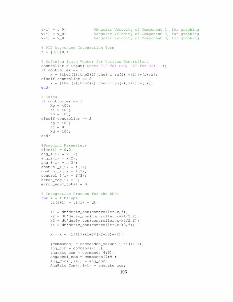
106

u(i) = u_0; %Angular Velocity of Component 1, for graphing v(i) = v_0; %Angular Velocity of Component 2, for graphing w(i) = w_0; %Angular Velocity of Component 3, for graphing % PID Augmented Integration Term z = [0;0;0]; % Defining State Vector for Various Controllers controller = input( 'Enter "1" for PID, "2" for DI: ' ); if controller == 1 x = [the1(i);the2(i);the3(i);u(i);v(i);w(i);z]; elseif controller == 2 x = [the1(i);the2(i);the3(i);u(i);v(i);w(i)]; end ; % Gains if controller == 1 Kp = 400; Ki = 400; Kd = 100; elseif controller == 2 Kp = 400; Ki = 0; Kd = 100; end ; %Graphing Parameters time(i) = 0.0; ang_1(i) = x(1); ang_2(i) = x(2); ang_3(i) = x(3); control_1(i) = f(1); control_2(i) = f(2); control_3(i) = f(3); error_mag(i) = 0; error_norm_total = 0; % Integration Process for the RK44 for i = 1:tsteps ti(i+1) = ti(i) + dt; k1 = dt*deriv_con(controller,x,f); k2 = dt*deriv_con(controller,x+k1/2,f); k3 = dt*deriv_con(controller,x+k2/2,f); k4 = dt*deriv_con(controller,x+k3,f); x = x + (1/6)*(k1+2*(k2+k3)+k4); [commands] = commanded_values(i,ti(i+1)); ang_com = commands(1:3); angrate_com = commands(4:6); angaccel_com = commands(7:9); Ang_Com(:,i+1) = ang_com; AngRate_Com(:,i+1) = angrate_com;

107

[f,error_norm] = control_develop(controller,i,x ); error_mag(i+1) = error_norm; error_norm_total = error_norm_total + error_nor m; ang_1(i+1) = x(1); ang_2(i+1) = x(2); ang_3(i+1) = x(3); control_1(i+1) = f(1); control_2(i+1) = f(2); control_3(i+1) = f(3); time(i+1) = ti(i+1); end ; error_norm_avg = error_norm_total/tsteps

*************************************************** **********

function [k]=Controller_Main(controller,x,f) global g d I1 I2 I3 m dt ang_com angrate_com I1x = I1(1,1); I1y = I1(2,2); I1z = I1(3,3); I2x = I2(1,1); I2y = I2(2,2); I2z = I2(3,3); I3x = I3(1,1); I3y = I3(2,2); I3z = I3(3,3); the1 = x(1); the2 = x(2); the3 = x(3); t1d = x(4); t2d = x(5); t3d = x(6); M11 = I1y + (I2x+I3x)*(sin(the2))^2 + (I2y + I3y*(c os(the3))^2 + I3z*(sin(the3))^2)*(cos(the2))^2; M12 = (I3y-I3z)*cos(the2)*cos(the3)*sin(the3); M21 = M12; M13 = I3x*sin(the2); M22 = I3y*(sin(the3))^2 + I3z*(cos(the3))^2 + I2z; M23 = 0; M31 = M13; M32 = M23; M33 = I3x; M = [M11 M12 M13; M21 M22 M23; M31 M32 M33];

108

h1 = (t2d^2)*sin(the2)*cos(the3)*sin(the3)*(I3z-I3y ) ... + t1d*t2d*2*cos(the2)*sin(the2)*(I2x-I2y+I3x -(I3y*(cos(the3))^2+I3z*(sin(the3))^2)) ... + t1d*t3d*(-2*(I3y-I3z)*cos(the3)*sin(the3)*(c os(the2))^2) ... + t2d*t3d*cos(the2)*(I3x+I3y*((cos(the3))^2 -(sin(the3))^2)+I3z*((sin(the3))^2-(cos(the3)) ^2)) ... + m*g*(-(sqrt(2)/2)*d*(((1-cos((pi/2)-the1))^( -1/2))*sin((pi/2) -the1)*sin((pi/4)-0.5*the1)+sqrt(1-cos((pi/2)- the1))*cos((pi/4) -0.5*the1))+d*(1-cos(the2))*sin((pi/2)-the1)); h2 = (t1d^2)*cos(the2)*sin(the2)*(I2y-I2x -I3x+I3y*(cos(the3))^2+I3z*(sin(the3))^2) ... + t1d*t3d*cos(the2)*(I3y*((cos(the3))^2 -(sin(the3))^2)+I3z*((sin(the3))^2-(cos(the3)) ^2)-I3x) ... + t2d*t3d*2*(I3y-I3z)*cos(the3)*sin(the3) ... + m*g*d*sin(the2)*cos((pi/2)-the1); h3 = (t1d^2)*(I3y-I3z)*(cos(the2))^2*cos(the3)*sin( the3) ... + (t2d^2)*(I3z-I3y)*cos(the3)*sin(the3) ... + t1d*t2d*cos(the2)*(I3x+I3y*((sin(the3))^2 -(cos(the3))^2)+I3z*((cos(the3))^2-(sin(the3)) ^2)); h = [h1;h2;h3]; ang_rate_dot = M\(f - h); if controller == 1 ang = [the1;the2;the3]; error = ang_com - ang; int_error = error; k = [t1d;t2d;t3d;ang_rate_dot;int_error]; elseif controller == 2 k = [t1d;t2d;t3d;ang_rate_dot]; end ;

*************************************************** **********

function [commands]=Controller_Main(i,t) global dt ang_com_temp angrate_com_temp % Commanded Angles and Rates for Sinusoidal Motion % ang_com = [0.5*sin(t);0.5*sin(t);0.5*sin(t)]; % angrate_com = [0.5*cos(t);0.5*cos(t);0.5*cos(t)]; % angaccel_com = [-0.5*sin(t);-0.5*sin(t);-0.5*sin( t)]; % Commanded Angles and Rates for Constant Motion ang_com = [0.1;0.1;0.2]; angrate_com = (ang_com - ang_com_temp)/dt; angaccel_com = (angrate_com - angrate_com_temp)/dt; ang_com_temp = ang_com; angrate_com_temp = angrate_com; % Step Function after a Given Time Period

109

% if i>=500 % ang_com = [0.2;0.2;0.5]; % end; commands = [ang_com;angrate_com;angaccel_com];

*************************************************** **********

function [ftemp,error_norm]=Controller_Main(controller,i,x) global ang_com angrate_com Kp Ki Kd ang = [x(1);x(2);x(3)]; vel = [x(4);x(5);x(6)]; angle_error = ang_com - ang; if i >= 0 error_norm = norm(angle_error); else error_norm = 0; end ; if controller == 1 e = ang_com - ang; de = angrate_com - vel; z_vec = [x(7);x(8);x(9)]; ftemp = Kp*e + Ki*z_vec + Kd*de; elseif controller == 2 [qr,qdr,Mr,hr,fr,q,qd,M,h]=model_components(ang ,vel); ftemp = M*(Mr\fr) + (h - M*(Mr\hr)) - M*(Kp*(q- qr)+Kd*(qd-qdr)); end ;

*************************************************** **********

function [qr,qdr,Mr,hr,fr,q,qd,M,h]=control_develop(the,vel ) global g d I1 I2 I3 m dt ang_com angrate_com angaccel_com I1x = I1(1,1); I1y = I1(2,2); I1z = I1(3,3); I2x = I2(1,1); I2y = I2(2,2); I2z = I2(3,3); I3x = I3(1,1); I3y = I3(2,2); I3z = I3(3,3);

110

%%%%%%%%%%%%%%%%%%%%% Reference Values %%%%%%%%%%%%%%%%%%%%%%%%%%% % Positional Variables the1r = ang_com(1); the2r = ang_com(2); the3r = ang_com(3); qr = [the1r;the2r;the3r]; % Velocity Variables t1dr = angrate_com(1); t2dr = angrate_com(2); t3dr = angrate_com(3); qdr = [t1dr;t2dr;t3dr]; % Acceleration Variables t1ddr = angaccel_com(1); t2ddr = angaccel_com(2); t3ddr = angaccel_com(3); tddr = [t1ddr;t2ddr;t3ddr]; % Returned Variables M11 = I1y + (I2x+I3x)*(sin(the2r))^2 + (I2y + I3y*( cos(the3r))^2 + I3z*(sin(the3r))^2)*(cos(the2r))^2; M12 = (I3y-I3z)*cos(the2r)*cos(the3r)*sin(the3r); M21 = M12; M13 = I3x*sin(the2r); M22 = I3y*(sin(the3r))^2 + I3z*(cos(the3r))^2 + I2z ; M23 = 0; M31 = M13; M32 = M23; M33 = I3x; Mr = [M11 M12 M13; M21 M22 M23; M31 M32 M33]; h1 = (t2dr^2)*sin(the2r)*cos(the3r)*sin(the3r)*(I3z -I3y) ...

+ t1dr*t2dr*2*cos(the2r)*sin(the2r)*(I2x-I2y+I3x- (I3y*(cos(the3r))^2+I3z*(sin(the3r))^2)) ...

+ t1dr*t3dr*(-2*(I3y-I3z)*cos(the3r)*sin(the3r )*(cos(the2r))^2) ... + t2dr*t3dr*cos(the2r)*(I3x+I3y*((cos(the3r))^ 2- (sin(the3r))^2)+I3z*((sin(the3r))^2-(cos(the 3r))^2)) ... + m*g*(-(sqrt(2)/2)*d*(((1-cos((pi/2)-the1r))^ (-1/2))*sin((pi/2) -the1r)*sin((pi/4)-0.5*the1r)+sqrt(1-cos((pi/2 ) -the1r))*cos((pi/4)-0.5*the1r))+d*(1-cos(the2r ))*sin((pi/2) -the1r)); h2 = (t1dr^2)*cos(the2r)*sin(the2r)*(I2y-I2x -I3x+I3y*(cos(the3r))^2+I3z*(sin(the3r))^2) ... + t1dr*t3dr*cos(the2r)*(I3y*((cos(the3r))^2 -(sin(the3r))^2)+I3z*((sin(the3r))^2-(cos(the3 r))^2)-I3x) ... + t2dr*t3dr*2*(I3y-I3z)*cos(the3r)*sin(the3r) ... + m*g*d*sin(the2r)*cos((pi/2)-the1r); h3 = (t1dr^2)*(I3y-I3z)*(cos(the2r))^2*cos(the3r)*s in(the3r) ... + (t2dr^2)*(I3z-I3y)*cos(the3r)*sin(the3r) ... + t1dr*t2dr*cos(the2r)*(I3x+I3y*((sin(the3r))^ 2

111

-(cos(the3r))^2)+I3z*((cos(the3r))^2-(sin(the3 r))^2)); hr = [h1;h2;h3]; fr = Mr*tddr + hr; %%%%%%%%%%%%%%%%%% Actual Values %%%%%%%%%%%%%%%%%%%% % Positional Variables the1 = the(1); the2 = the(2); the3 = the(3); q = [the1;the2;the3]; % Velocity Variables t1d = vel(1); t2d = vel(2); t3d = vel(3); qd = [t1d;t2d;t3d]; % Returned Variables M11 = I1y + (I2x+I3x)*(sin(the2))^2 + (I2y + I3y*(c os(the3))^2 + I3z*(sin(the3))^2)*(cos(the2))^2; M12 = (I3y-I3z)*cos(the2)*cos(the3)*sin(the3); M21 = M12; M13 = I3x*sin(the2); M22 = I3y*(sin(the3))^2 + I3z*(cos(the3))^2 + I2z; M23 = 0; M31 = M13; M32 = M23; M33 = I3x; M = [M11 M12 M13; M21 M22 M23; M31 M32 M33]; h1 = (t2d^2)*sin(the2)*cos(the3)*sin(the3)*(I3z-I3y ) ... + t1d*t2d*2*cos(the2)*sin(the2)*(I2x-I2y+I3x -(I3y*(cos(the3))^2+I3z*(sin(the3))^2)) ... + t1d*t3d*(-2*(I3y-I3z)*cos(the3)*sin(the3)*(c os(the2))^2) ... + t2d*t3d*cos(the2)*(I3x+I3y*((cos(the3))^2 -(sin(the3))^2)+I3z*((sin(the3))^2-(cos(the3)) ^2)) ... + m*g*(-(sqrt(2)/2)*d*(((1-cos((pi/2)-the1))^( -1/2))*sin((pi/2) -the1)*sin((pi/4)-0.5*the1)+sqrt(1-cos((pi/2)- the1))*cos((pi/4) -0.5*the1))+d*(1-cos(the2))*sin((pi/2)-the1)); h2 = (t1d^2)*cos(the2)*sin(the2)*(I2y-I2x -I3x+I3y*(cos(the3))^2+I3z*(sin(the3))^2) ... + t1d*t3d*cos(the2)*(I3y*((cos(the3))^2 -(sin(the3))^2)+I3z*((sin(the3))^2-(cos(the3)) ^2)-I3x) ... + t2d*t3d*2*(I3y-I3z)*cos(the3)*sin(the3) ... + m*g*d*sin(the2)*cos((pi/2)-the1); h3 = (t1d^2)*(I3y-I3z)*(cos(the2))^2*cos(the3)*sin( the3) ... + (t2d^2)*(I3z-I3y)*cos(the3)*sin(the3) ... + t1d*t2d*cos(the2)*(I3x+I3y*((sin(the3))^2 -(cos(the3))^2)+I3z*((cos(the3))^2-(sin(the3)) ^2)); h = [h1;h2;h3];

nonlinear tracking of natural mechanical systems for hwil

Documents