optimal tracking control of nonlinear dynamical...

on June 3, 2018http://rspa.royalsocietypublishing.org/Downloaded from

Optimal tracking control of nonlineardynamical systems

BY FIRDAUS E. UDWADIA*,1,2,3,4,5

1Department of Aerospace and Mechanical Engineering, 2Department ofCivil and Environmental Engineering, 3Department of Mathematics,

4Systems Architecture Engineering, and 5Information andOperations Management, University of Southern California,

430K Olin Hall, Los Angeles, CA 90089-1453, USA

This paper presents a simple methodology for obtaining the entire set of continuouscontrollers that cause a nonlinear dynamical system to exactly track a given trajectory.The trajectory is provided as a set of algebraic and/or differential equations that may ormay not be explicitly dependent on time. Closed-form results are also provided for the real-time optimal control of such systems when the control cost to be minimized is any givenweighted norm of the control, and the minimization is done not just of the integral of thisnorm over a span of time but also at each instant of time. The method provided is inspiredby results from analytical dynamics and the close connection between nonlinear controland analytical dynamics is explored. The paper progressively moves from mechanicalsystems that are described by the second-order differential equations of Newton and/orLagrange to the first-order equations of Poincare, and then on to general first-ordernonlinear dynamical systems. A numerical example illustrates the methodology.

Keywords: exact control; tracking control; nonlinear systems

*AdSou

RecAcc

1. Introduction

Thedevelopment of controllers for nonlinearmechanical systemshas been an area ofintense research over the last two decades or so. Many controllers that have beendeveloped for trajectory tracking of complex nonlinear andmulti-body systems relyon some approximations and/or linearizations (Slotine & Li 1991; Sastry 1999;Naidu 2003). Most control designs restrict controllers for nonlinear systems to beaffine in the control inputs (Brogliato et al. 2007). Often, the system equations arelinearized about the system’s nominal trajectory and then the linearized equationsare used alongwith various results from thewell-developed theories of linear control.While this often works well in many situations, there are some situations in whichbetter controllers may be needed. This is especially so when highly accuratetrajectory tracking is required to be done in real time on systems that are highlynonlinear. Examples include the exact trajectory control of orbital, attitudinal andelastic motions of a multi-body spacecraft system that is required to performprecision tumbling.

Proc. R. Soc. A (2008) 464, 2341–2363

doi:10.1098/rspa.2008.0040

Published online 24 April 2008

dress for correspondence: Department of Aerospace and Mechanical Engineering, University ofthern California, 430K Olin Hall, Los Angeles, CA 90089-1453, USA ([email protected]).

eived 28 January 2008epted 28 March 2008 2341 This journal is q 2008 The Royal Society

http://rspa.royalsocietypublishing.org/

F. E. Udwadia2342


To place this paper within the context of the enormous literature that hasbeen generated in the area of tracking control of nonlinear systems and tohighlight what is new in it, we provide a brief review of the methods that havebeen developed so far and that have been applied to numerous areas ofapplication ranging from chemical process control to robotics. Brogliato et al.(2007) provide an exhaustive review of the methods that have been developed todate for the tracking control of systems along with over 500 references. Theypoint out that methods developed to date rely heavily on PID-type control and,most often, a linear feedback is provided to track a given trajectory. Chaou &Chang (2004) also provide recent developments on trajectory tracking and dealwith the same basic theme (linear feedback) along with numerous applications.The optimality criterion considered in the literature to date is the minimizationof the control cost integrated over a suitable span of time. In the roboticsliterature (Brogliato et al. 2007), trajectory tracking using inverse dynamics andmodel reference control has been used for some time now, and the methodsdeveloped therein can be seen as particular subclasses of the formulationdiscussed in the present work. Nonlinear control methods using controlledLagrangian and Hamiltonians have also been explored along with passivitytheory (Brockett 1977). These methods limit the structure of the control for amechanical system to be a nonlinear function of its generalized displacement andthey usually do not address the issue of control optimality. No such assumptionsare made in this paper. Trajectory tracking in the adaptive control context(which is not the subject of this paper) has also been explored together withspecific parametrizations to guarantee linearity in the unknown parameters ofa system (Sadegh 1990). Thus, the methods used to date primarily rely onlinearizations and/or PID-type control, and they posit assumptions on thestructure of the control effort.

By contrast, this paper takes a widely different approach that is based onrecent results from analytical dynamics. Here the complete nonlinear problem isaddressed with no assumptions on the type of controller that is to be used, exceptthat it be continuous. In particular, we do not posit that the control is affine inthe inputs, we do not use linearized equations of motion about the desiredtrajectory, nor do we assume any ‘feedback structure’ to the nonlinear controleffort. Furthermore, the optimality criterion used is the minimization of thecontrol cost at each instant of time. As far as is known, the results provided hereyield new and explicit methods for the control of highly nonlinear systems.Moreover, we provide for the first time the entire class of nonlinear Lipschitz-continuous (LC) controllers that would track the desired trajectory of thesystem, and we identify from among these controllers the one that minimizes, ateach instant of time, a specified weighted norm of the control effort.

Since we illustrate the power of the technique developed herein to ensure thetracking of a Rossler chaotic system by another Lorenz chaotic system, it isappropriate to indicate the state of the art in synchronization of nonlinearchaotic systems. Nearly all the work that has been done to date on thesynchronization of chaotic systems deals with synchronization of identicalchaotic oscillators that start from different initial conditions. This synchroniza-tion is performed by linear feedback between one or more of the phase states ofthe system (see Chen 2002; Lei et al. 2005). A recent monograph (with 350references) points this out in detail (Boccaletti et al. 2002). It is only very

Proc. R. Soc. A (2008)


2343Tracking control of nonlinear systems


recently that the synchronization between two non-identical, low-dimensionalchaotic systems has begun to be investigated (Boccaletti et al. 2002). One of thefew papers on this is by Pyras (1996), which uses linear feedback. Rulkov et al.(1995) showed that this type of synchronization could exist. Such synchroniza-tion studies have resulted in the so-called imperfect phase synchronization (Zakset al. 1999) in which the systems get ultimately de-synchronized by havingintermittent phase slips, and lag synchronization (Rosenblum et al. 1997) whichresults in a time lag between the synchronized systems. Linear feedback has beenused in all these studies, with the aim of synchronizing all the states ofone chaotic system with those of the other. In our example we use non-identicalchaotic systems. Our methodology does not assume any a priori structure on thecontrol for the synchronization; no restrictions on the chaotic systems being oflow dimensionality is required; as illustrated in the example, we can opt tosynchronize (at will) one or more of the phase space variables; and, we can obtainthe entire set of controllers in closed form that would do the job. Finally, amongall these controllers, in the example we show that we can explicitly provide thecontroller that synchronizes and minimizes a weighted norm of the control effortat each instant of time.

We begin by reformulating the trajectory control problem as a problem ofconstrained motion in the Lagrangian framework and use the underlyinginspiration with which constrained motion in analytical dynamics is orchestratedby Nature (Udwadia & Kalaba 2002). We then expand and further develop thisview by first considering mechanical systems described by first-order Poincareequations and then general nonlinear systems. Closed-form expressions for all thecontinuous controllers required for trajectory tracking for nonlinear systems thatdo not make approximations, either in describing the nonlinear system or in thenature of the nonlinear controller employed, are obtained. Such closed-formresults appear to be new. Furthermore, no approximations or linearizations aremade here with respect to the trajectory that is being tracked, which may bedescribed in terms of nonlinear algebraic equations, nonlinear differentialequations or a combination thereof; these descriptions could explicitly involvetime also. Moreover, the approach arrives not just at one nonlinear controller forcontrolling a given nonlinear system, but also at the entire set of continuouscontrollers that would cause a given set of trajectory descriptions to be exactlysatisfied. Furthermore, we show that when the cost function is the weightednorm of the generalized control input, its minimization can be done to yield theoptimal controller that minimizes not just the integrated cost over a span oftime, but also the cost at each instant of time. Explicit closed-form expressionsfor the optimal control are obtained.

Section 2a of this paper begins with mechanical systems described by thesecond-order differential equations of the Newtonian and/or Lagrangianmechanics. Section 2b deals with Poincare’s first-order differential equationsthat describe the motion of mechanical systems; this takes us a step furthertowards general first-order nonlinear dynamical systems. Section 3 deals with theclose connection that the set of controllers developed in §2 have with the wayNature seems to orchestrate the control of mechanical systems subjected totrajectory requirements (constraints). The development of such controllersand their close correspondence with (i) Gauss’s principle of least constraint and(ii) the recently developed equations of motions for non-ideal constraints



F. E. Udwadia2344


are provided. Lessons from the way Nature seems to control mechanical systemsare adduced. Section 4 deals with the exact control of general dynamicalsystems described by a set of nonlinear, non-autonomous ordinary differentialequations. Section 5 deals with a numerical example that demonstrates theclosed-form development of the control required to be applied to a nonlinearchaotic dynamical system so that it tracks the motions of another differentnonlinear chaotic system. Section 6 concludes the paper with some remarksand observations.

2. Development of the entire set of controllers that cause a mechanicalsystem to track a given trajectory

(a ) Lagrangian and Newtonian descriptions

Consider an unconstrained nonlinear mechanical system described by the second-order differential equation of motion

Mðq; tÞ€q ZQðq; _q; tÞ; qð0ÞZ q0; _qð0ÞZ _q0; ð2:1Þwhere q(t) is the n-vector (n by 1 vector) of generalized coordinates; the dotsindicate differentiation with respect to time; and the matrix M(q, t) is a positive-definite n by n matrix. Equation (2.1) can be obtained using either Newtonianor Lagrangian mechanics (Lagrange 1811; Hamel 1949; Goldstein 1976). Then-vector Q on the r.h.s. of equation (2.1) is a ‘known’ vector in the sense that itis a known function of its arguments. By ‘unconstrained’ we mean that thecomponents of the initial velocity _q0 of the system can be independently assigned.

We next require that this mechanical system be controlled so that it tracks atrajectory that is described by the following consistent set of m equations:

fiðq; tÞZ 0; i Z 1;.; h ð2:2Þand

jiðq; _q; tÞZ 0; i Z hC1;.;m: ð2:3ÞWe shall assume that the mechanical system’s initial conditions are such as tosatisfy these relations at the initial time. The latter set of equations, which arenon-integrable, is non-holonomic (Hamel 1949).

In order to control the system so that it exactly tracks the requiredtrajectory—i.e. satisfies equations (2.2) and (2.3)—we apply an appropriatecontrol n-vector Qcðq; _q; tÞ, so that the equation of motion of the controlledsystem becomes

Mðq; tÞ€q ZQðq; _q; tÞCQcðq; q; tÞ; qð0ÞZ q0; _qð0ÞZ _q0; ð2:4Þ

where now the components of the n-vectors q0 and _q0 satisfy equations (2.2) and(2.3) at the initial time, tZ0. Throughout this paper, we shall, for brevity, dropthe arguments of the various quantities, unless needed for clarity.

We begin by expressing equation (2.4) in terms of the weighted accelerationsof the system. For any positive-definite n by n matrix N(q, t), we definethe matrix

Gðq; tÞd½N 1=2ðq; tÞMðq; tÞ�K1 ZMK1ðq; tÞNK1=2ðq; tÞ; ð2:5Þ





and pre-multiplying equation (2.4) by N1/2 (q, t), the ‘scaled’ equation, which wedenote using the subscript ‘s’, is obtained as

€q s Z as C€q cs ; ð2:6Þ

where

€q sdGK1€q ; ð2:7Þ

a sdGK1a Z ðN 1=2MÞðMK1QÞZN 1=2Q ð2:8Þand

€q cs dGK1€q c Z ðN 1=2MÞðMK1QcÞZN 1=2Qc: ð2:9Þ

In equation (2.8), we denote the acceleration of the uncontrolled system byaðq; _q; tÞZMK1ðq; tÞQðq; _q; tÞ: In equation (2.9), €q cðq; _q; tÞZMK1ðq; tÞQcðq; _q; tÞcan be viewed as the deviation of the acceleration of the controlled system fromthat of the uncontrolled system. We now differentiate equation (2.2) twice withrespect to time t, and equation (2.3) once with respect to time, giving the setof equations

Aðq; _q; tÞ€q Z bðq; _q; tÞ; ð2:10Þwhere A is an m by n matrix of rank k and b is an m-vector. Noting equation(2.7), equation (2.10) can be further expressed as

Bsðq; _q; tÞ€q s Z bðq; _q; tÞ; ð2:11Þwhere Bsðq; _q; tÞdAðq; _q; tÞGðq; tÞ. We now express the n-vector €q s in terms of itsorthogonal projections on the range space of BT

s and the null space of Bs, so that

€q s ZBCs Bs€q sCðIKBC

s BsÞ€q s: ð2:12ÞIn equation (2.12), the matrix XC denotes the Moore–Penrose (MP) generalizedinverse of the matrix X (Moore 1910; Penrose 1955). It should be noted thatequation (2.12) is a general identity that is always valid since it arises from theorthogonal partition of the identity matrix IZBC

s BsCðIKBCs BsÞ. Using

equation (2.11) in the first member on the r.h.s. of equation (2.12), and equation(2.6) to replace €q s in the second member, we get

€q s ZBCs bCðIKBC

s BsÞða sC€q cs Þ; ð2:13Þ

which, owing to equation (2.6), yields

BCs Bs€q

cs ZBC

s ðbKBsa sÞ: ð2:14ÞBut the general solution of the linear set of equations (2.14) is given by(Graybill 2001)

€q cs Z ðBC

s BsÞCBCs ðbKBsa sÞC ½IKðBC

s BsÞCðBCs BsÞ�z

ZBCs ðbKBsa sÞCðIKBC

s BsÞz; ð2:15Þwhere the n-vector zðq; _q; tÞ is any arbitrary n-vector. In the second equalityabove, we have used the property that ðBC

s BsÞCZBCs Bs in the twomembers on the

r.h.s., along with the second MP-inverse property that BCs BsB

Cs ZBC

s . Usingequation (2.9), the explicit control force that exactly tracks the trajectoryby exactly satisfying the given relations (2.2) and (2.3) is then explicitly given by

Qc ZNK1=2€q cs ZNK1=2BC

s ðbKBsa sÞCNK1=2ðIKBCs BsÞz; ð2:16Þ



F. E. Udwadia2346


where Bsðq; _q; tÞdAðq; _q; tÞGðq; tÞ. We may take zðq; _q; tÞ to be C 1 (or, moregenerally, Lipschitz continuous (LC)) to ensure a unique solution to the system ofequations (2.4). We hence have the following result.

Result 2.1. Consider the mechanical system, which is described by theLagrange (or Newtonian) equations of motion

Mðq; tÞ€q ZQðq; _q; tÞ; ð2:17Þ

where M is an n by n positive-definite matrix and q is an n-vector. The system isrequired to exactly track the trajectory described by the equations

fiðq; tÞZ 0; i Z 1;.; h ð2:18Þand

jiðq; _q; tÞZ 0; i Z hC1;.;m: ð2:19ÞThe controlled system is described by the relation

Mðq; tÞ€q ZQðq; _q; tÞCQcðq; _q; tÞ; ð2:20Þwhere Qc is the control.

Assuming that the initial conditions of the mechanical system satisfy thesetrajectory requirements, the set of all possible controls Qcðq; _q; tÞ (or controllers)that causes the controlled system (2.20) to exactly track the required trajectoryis explicitly given by

Qc ZNK1=2BCs ðbKBsa sÞCNK1=2ðIKBC

s BsÞz; ð2:21Þ

where zðq; _q; tÞ is any arbitrary n-vector whose components are continuouslydifferentiable—or LC—functions of its arguments; N(q, t) is any arbitrary n by n

positive-definite matrix a sZN 1=2Q; Bsðq; _q; tÞZAðq; _q; tÞ½N 1=2ðq; tÞMðq; tÞ�K1 isan m by n matrix; Aðq; _q; tÞ is an m by n matrix of rank k, and bðq; _q; tÞ is them-vector defined in equation (2.10).

We can abbreviate the two components of the control vector Qcðq; _q; tÞ givenin equation (2.21) as

Qcðq; _q; tÞZQc1ðq; _q; tÞCQc

2ðq; _q; tÞ; ð2:22Þ

where

Qc1ðq; _q; tÞdNK1=2BC

s ðbKBsa sÞ; ð2:23Þand

Q c2 ðq; _q; tÞdNK1=2ðIKBC

s BsÞz: ð2:24Þ

Corollary 2.2. Relation (2.23) can also be given as

Qc1 ZNK1=2ðAMK1NK1=2ÞCðbKAaÞ: ð2:25Þ

Proof. Using the relation BsZAGZAMK1NK1=2 and equation (2.8), we haveBsa sZAGGK1aZAa, where aðq; _q; tÞZMK1ðq; _q; tÞQðq; _q; tÞ is the accelerationof the uncontrolled system. The result then follows. &





Remark 2.3. Owing to the generality of the decomposition (2.13), relation(2.21) (alternatively, relations (2.22)–(2.24)) provides the entire set ofcontinuous tracking controllers that cause the system to track the trajectorydescribed by equations (2.18) and (2.19).

Remark 2.4. The explicit closed-form tracking control obtained in equation(2.21), which causes the system to exactly track the given trajectory described byequations (2.18) and (2.19), does not contain any Lagrange multipliers, nor doesour derivation invoke the notion of a Lagrange multiplier.

We shall next show the following, somewhat remarkable, result.

Result 2.5. We again consider the mechanical system described by thenonlinear Lagrange or Newtonian equation (2.17), which needs to be controlledthrough the addition of a control, n -vector Qcðq; _q; tÞ, so that the trajectorydescribed by equations (2.18) and (2.19) is exactly tracked. Assuming that thesystem satisfies the trajectory requirements initially, the optimal controller thatcauses the system to

(i) exactly track the required trajectory and(ii) minimize at each instant of time t, the cost

Jðt ÞZ ½Qcðq; _q; tÞ�TNðq; tÞQcðq; _q; tÞ; ð2:26Þ

for a given n by n positive-definite matrix N, is explicitly provided by

Qcðq; _q; tÞZNK1=2BCs ðbKBsa sÞZNK1=2BC

s ðbKAaÞ; ð2:27Þ

where Bs, b and as are as defined before.

Proof. Let us define the vector

rðtÞdN 1=2Qc: ð2:28Þ

We note that by equation (2.26),

JðtÞZ ½Qcðq; q; tÞ�TNðq; tÞQcðq; q; tÞZ krðt Þk2: ð2:29Þ

Then in view of equation (2.20), equation (2.28) can be rewritten as

rðt ÞdN 1=2ðM €qKQÞ; ð2:30Þ

so that we obtain, using equation (2.8),

€q Z ½N 1=2M �K1ðr CN 1=2QÞZGðr Ca sÞ: ð2:31Þ

We assume that at the initial time the values of q0 and _q0 satisfy the trajectoryrequirements, and upon differentiating equations (2.18) and (2.19) we have,as before,

A€q Z b: ð2:32Þ

Using relation (2.31) and denoting BsZAG, equation (2.32) becomes

Bsr Z bKBsa s: ð2:33Þ



F. E. Udwadia2348


The solution of equation (2.33), subject to the condition that JðtÞZkrðtÞk2 is aminimum, is then given by (Graybill 2001)

rðt ÞZBCs ðbKBsa sÞ; ð2:34Þ

from which we obtain, by using relation (2.28), the explicit expression for theoptimal control as

Qcðq; _q; tÞZ ½Nðq; tÞ�K1=2BCs ðq; _q; tÞ½bðq; _q; tÞKBsðq; _q; tÞa sðq; _q; tÞ�; ð2:35Þ

where we have written out the explicit result in extensio. The second equality inequation (2.27) follows from corollary 2.2. &

Remark 2.6. For a given choice of the weighting matrix N, we have obtainedthe explicit closed-form expression for the exact full state controller that tracksthe trajectory described by equations (2.18) and (2.19) and minimizes the costfunction JðtÞZ ½Qc�TNðq; tÞQc, under the proviso that the initial conditions ofthe system satisfy the trajectory description. The minimum cost J(t) is given by

JðtÞZ ½Qc1�TNQc

1 Z kBCs ðbKAaÞk2 Z kðAMK1NK1=2ÞCðbKAaÞk2: ð2:36Þ

Note, as before, that the explicit result given in equation (2.27) does not containany Lagrange multipliers, nor does our derivation invoke anywhere the notion ofa Lagrange multiplier.

Remark 2.7. Result 2.5 and equation (2.23) show that for a given positive-definite matrix N(q, t) the optimal control that minimizes J(t) at each instant oftime is explicitly obtained in closed form by setting Q c

2 ðq; _q; tÞh0 in equation(2.22). One way (see corollary 2.8 below) of doing this would be by settingzðq; _q; tÞh0 in equation (2.24) (or, in equation (2.21)). More precisely, we havethe following result.

Corollary 2.8. At any instant of time t, at which the arbitrary LC vector zðq; _q; tÞbelongs to the range space of BT

s ðq; _q; tÞ, the control given by (2.21) becomes optimal,in the sense that it minimizes J(t) at that time.

Proof. When zðq; _q; tÞ belongs to the range space of BTs ðq; _q; tÞ at time t, we can

give zZBTs g for some m-vector g. Hence, by equation (2.24), Qc

2ðq; _q; tÞ becomes,

Q c2 dNK1=2ðIKBC

s BsÞz ZNK1=2½IKBCs Bs�BT

s g

ZNK1=2½IKðBCs BsÞT�BT

s gZNK1=2½IKBTs ðBC

s ÞT�BTs gZ 0: ð2:37Þ

The second equality follows from the fourth MP-inverse property, and the lastequality follows from the first MP-inverse property (Graybill 2001). &

Corollary 2.9. (i) The two components Q c1 and Q c

2 of the control vectorQc given in equation (2.22) are N-orthogonal to one another and (ii) Q c

1 is(MN )-orthogonal to the null space of the matrix A.





Proof.(i) Since

½Qc2�TNQc

1 Z zTðIKBCs BsÞTNK1=2NNK1=2BC

s ðbKBsa sÞ

Z zTðIKBCs BsÞBC

s ðbKBsasÞZ 0: ð2:38Þ

The result follows by using the fourth and then the second MP-inverse property(Graybill 2001).

(ii) Substituting for Bs and using the identity XCZXTðXXTÞC we get

NK1=2BCs ZNK1=2ðAMK1NK1=2ÞC

ZNK1=2ðAMK1NK1=2ÞT½ðAMK1NK1=2ÞðAMK1NK1=2ÞT�C

Z ðMNÞCATðAMK1NK1MK1ATÞC: ð2:39Þ

Any vector belonging to the null space of the matrix A satisfies the relationAvZ0, whose explicit solution is

v Z ðIKACAÞw; ð2:40Þwhere w is any n-vector. Hence

vTMNQc1 ZwTðIKACAÞTðMNÞðMNÞK1ATðAMK1NK1MK1ATÞCðbKBsa sÞZwT½IKATðATÞC�ATðAMK1NK1MK1ATÞCðbKBsa sÞZ 0; ð2:41Þ

since ½IKATðATÞC�ATZ0. &

Corollary 2.10. The component Q c1 as defined in (2.23) belongs to the range

space of the matrix NK1=2BCs , and the component Q c

2 as defined in equation (2.24)is N-orthogonal to the range space of NK1=2BT

s .

Proof. The first result is obvious from the expression for Qc1 in equation (2.23).

The second follows because any vector a in the range space of NK1=2BTs can be

expressed as

aZNK1=2BTs g; ð2:42Þ

for some m-vector g, and so

aTNQc2 ZgTBsN

K1=2NNK1=2ðIKBCs BsÞz Z 0: ð2:43Þ

Hence the result. &

We note that the range space of NK1=2BCs is the same as the range space of

NK1=2BTs . This follows because for any vector g, we can always find a vector a

such that NK1=2BTs aZNK1=2BC

s g, and vice-versa.

Remark 2.11. The addition of the second component Q c2 to the control so that

Q cZQc1CQ c

2 , whatever the LC n-vector z may be, still ensures that thedescription of the trajectory given by equations (2.18) and (2.19) is exactlysatisfied. However, it contributes an additional amount given by kðIKBC

s BsÞzk2 tothe cost of the control, since the two components Q c

1 and Q c2 are N-orthogonal



F. E. Udwadia2350


to each other (corollary 2.9). Furthermore, if at any time t the function zðq; _q; tÞbelongs to the null space of Bs this additional cost at that time simplybecomes kzk2.

It is sometimes advantageous to describe the motion in terms of a system offirst-order differential equations instead of a system of second-order equations.One obvious way of doing this is to define a new variable, an n-vector vZ _q, sothat the equation of motion takes the so-called state space form given by

_q Z v; qð0ÞZ q0; ð2:44aÞ

Mðq; tÞ _v ZQðq; v; tÞ; vð0ÞZ v0: ð2:44bÞThe first equation of this set is simply a definition, whereas the second equationof the set is the one that contains the actual dynamics. And while this is the formoften used when numerically integrating equation (2.1), the description of themotion of a mechanical system in terms of a system of first-order differentialequations goes far beyond just its use in numerical procedures. For, often thesefirst-order descriptions (i.e. descriptions using first-order differential equations)arise when one wants to use descriptions of motion in terms of coordinates thatmay be more physically meaningful in the context of a particular problem. Forexample, the first-order Hamilton’s equations describing the motion ofmechanical systems are often useful when dealing with systems described by aHamiltonian, and, more generally, the first-order set of Poincare equations areoften useful when dealing with rigid body and multi-body dynamics. We nextobtain the entire set of explicit closed-form controllers for exactly tracking thetrajectory of mechanical systems described by Poincare’s equations of motion.

(b ) Poincare descriptions

The Poincare equations (Poincare 1901) are obtained by defining a newvariable, an n-vector sZ ~Hðq; tÞ _q, where ~Hðq; tÞ is a non-singular matrix whoseelements are known functions of q and t. Denoting the inverse of the matrix ~H byH(q, t), so that _qZHðq; tÞs, the Lagrange equation (2.1) can be rewritten infirst-order form as (Udwadia & Phohomsiri 2007)

_q ZHðq; tÞs; qð0ÞZ q0; ð2:45Þ

Mpðq; tÞ_sZSðq; s; tÞ; sð0ÞZ s0; ð2:46Þ

where the state variables are now the n-vectors q and s. In rigid body dynamics,the 3-vector s is often chosen to constitute the three components of the angularvelocity of the body. Here the matrix Mp is again positive definite. Though bothfirst-order equations are, mathematically speaking, on a par, the first equationof the set (equation (2.45)) is a kinematic relation involving the definition ofthe new variable s—hence, an identity as in equation (2.44a)—while the secondequation (equation (2.46)) is the dynamical equation of motion. The system isrequired to track the trajectory described by the consistent relations

fpi ðq; tÞZ 0; i Z 1;.; h; ð2:47Þ

jpi ðq; s; tÞZ 0; i Z h Z 1;.;m: ð2:48Þ





The subscripts and superscripts ‘p’ indicate that we are dealing with thePoincare description of the motion of the dynamical system. In order to controlthe system so that it exactly tracks this trajectory, we apply a control so thatthe equation of motion of the controlled system now becomes

_q ZHðq; tÞs; qð0ÞZ q0; ð2:49ÞMpðq; tÞ_sZSðq; s; tÞCS cðq; s; tÞ; sð0ÞZ s0; ð2:50Þ

and the initial conditions q0 and s0 satisfy the trajectory requirements (2.47) and(2.48). The explicit expression for the control force, yielding the entire set of allcontrollers that will cause the dynamical system described by equations (2.45)and (2.46) to track the required trajectory described by equations (2.47) and(2.48) will now be obtained.

As before, we define the matrix

Gpðq; tÞd½NK1=2ðq; tÞMpðq; tÞ�K1 ZMK1p ðq; tÞNK1=2ðq; tÞ; ð2:51Þ

where the matrix N(q, t) is any positive-definite matrix, and the scaled variables

_ss ZGK1p _s;

a s ZGK1p a Z ðN 1=2MpÞðMK1

p SÞZN 1=2Sand

_scs ZN 1=2S c;

9>>>>=>>>>;

ð2:52Þ

so that relation (2.50) on pre-multiplication with N 1/2 becomes

_ss Z a sC _s cs ; ð2:53Þwhich we note is of the same form as equation (2.6), except that we now have sinstead of q, and first derivatives instead of second derivatives with respectto time.

On differentiating equation (2.47) twice with respect to time and differentia-ting equation (2.48) once with respect to time, and using relation (2.49), we thenobtain the matrix equation

Apðq; s; tÞ_sZ bpðq; s; tÞ; ð2:54Þ

which, upon using the first equation of the set (2.52), can be rewritten as

Bsðq; s; tÞ_ss Z bpðq; s; tÞ; ð2:55Þ

where we define the m by n matrix Bs of rank k by the relation

Bsðq; s; tÞZApðq; s; tÞGpðq; tÞ: ð2:56Þ

Again we note the similarity between equations (2.10) and (2.11) and equations(2.54) and (2.55). We next decompose the n-vector _ss as

_ss ZBCs Bs _ss CðIKBC

s BsÞ _ss; ð2:57Þin a manner similar to equation (2.12), with the matrix Bs now definedby equation (2.56). Proceeding along with similar lines as before (equations(2.13)–(2.16)), we then find that

Sc ZNK1=2 _s cs ZNK1=2BCs ðbpKBsa sÞCNK1=2ðIKBC

s BsÞzpdS c1CS c

2; ð2:58Þ



F. E. Udwadia2352


where zpðq; s; tÞ is any arbitrary n -vector. To ensure a unique solution ofequations (2.49) and (2.50), we may then take the components of zpðq; s; tÞ tobe C 1 functions (or, more generally, LC functions) of q, s and t.

Following the same lines as in §2a, for any Poincare system described byequation (2.45) that is required to exactly track the trajectory described byrelations (2.47) and (2.48), we now obtain results that are analogous to thosegiven in results 2.1 and 2.5. Using as defined in relation (2.52), and Bs in (2.56),we simply make the following variable changes: _q/s, Q/S, b/bp , M/Mp,

z/zp,A/Ap, andG/Gp, in the expressions given in equations (2.21) and (2.27)to obtain the corresponding control forces.

Remark 2.12. We can prove corollaries similar to corollaries 2.2, 2.8–2.10. Thesame goes for remarks 2.3, 2.4, 2.6, 2.7, 2.11.

3. The close connection between nonlinear control andanalytical dynamics

Since almost all mechanical systems are nonlinear in their behaviour, includingeven simple ones like a pendulum, we will be mainly addressing nonlinear systemshere. The problem of control can be placed within the context of analyticalmechanics by reinterpreting constrained motion in mechanical systems. Considera mechanical system described by equation (2.17). When the system is furthersubjected to the trajectory requirements (2.18) and (2.19)—i.e. subjected tofurther constraints—additional control (constraint) forces are brought into playby Nature so that the controlled (constrained) system moves in such a mannerthat it satisfies these trajectory requirements (constraints). Thus, the additionalcontrol (constraint) Qcðq; _q; tÞ that Nature provides may be thought of as thecontrol it generates in order for the system to satisfy the trajectory requirementsgiven by equations (2.18) and (2.19). One might imagine Nature as a controlengineer, attempting to control the mechanical system so that it satisfies thegiven trajectory requirements described by equations (2.18) and (2.19). However,to entertain such an interpretation, one is led to ask the following three questions.

(i) To what extent might Nature be perceived as acting like a control engineer?(ii) Does Nature appear to be performing the control in any kind of an optimal

manner?(iii) If so, what is the cost function (or functional) it appears to minimize?

We shall start answering these questions by first asserting that Nature appearsto choose the weighting matrix Nðq; tÞZ ½Mðq; tÞ�K1dNNatureðq; tÞ in equation(2.21). Here M is the so-called ‘mass matrix’ and appears on the l.h.s. ofequation (2.17).

Result 3.1. Nature seems to control a mechanical system described byequation (2.17), so it exactly satisfies the trajectory described by therequirements (2.18) and (2.19) by choosing the weighting matrix to be

Nðq; tÞZ ½Mðq; tÞ�K1: ð3:1Þ





Proof. Setting Nðq; tÞZ ½Mðq; tÞ�K1 equation (2.21) now yields

Qcðq; _q; tÞZM 1=2BCðbKAaÞCM 1=2ðIKBCBÞz; ð3:2Þ

where BdAGZAMK1=2 and BsasZAGGK1aZAa. But equation (3.2) isexactly the equation of motion of a general constrained mechanical system, asgiven by Udwadia (2000) and Udwadia & Kalaba (2002). Hence the result. &

Result 3.2. If we assume that Nature observes d’Alembert’s principle, then itappears to be minimizing the cost

JNatureðt ÞZ ½Qcðq; _q; tÞ�T ½Mðq; tÞ�K1Qcðq; _q; tÞ; ð3:3Þat each instant of time while controlling the system defined by equation (2.17) soit exactly satisfies the trajectory described by the requirements (2.18) and (2.19).

Proof. Setting Nðq; tÞZ ½Mðq; tÞ�K1 in result 2.5, equation (2.27), which givesthe optimal control while minimizing J(t), yields

Qcðq; _q; tÞZM 1=2BCðbKAaÞZQc1: ð3:4Þ

Using this expression for Qc in equation (2.20), we find that we obtain the correctequation of motion of a constrained mechanical system that obeys d’Alembert’sprinciple, as given by Udwadia & Kalaba (1992, 1996). &

Remark 3.3. Result 3.2 connects directly with the basic principles ofanalytical dynamics. In fact, d’Alembert’s principle, which is a principle thatleads to a mathematical description of motion, which is in close conformity withobservations, andwhich is one of the pivotal assumptions of analytical dynamics, isequivalent to Gauss’s principle (Gauss 1829; Udwadia & Kalaba 1996). AndGauss’s principle states that: of the entire set of constraint (control) forces thatcause a constrained (controlled) mechanical system (2.17) to exactly satisfy theconstraints (trajectory) described by requirements (2.18) and (2.19), Nature seemsto choose that constraint force that minimizes JNature (t) at each instant of time.

Thus we find that (i) Nature seems to choose the weighting matrix Nðq; tÞZ½Mðq; tÞ�K1 and (ii) if we assume that d’Alembert’s principle is true, thenNature seems to pick the one controller given in result 3.2 that minimizes thecost JNature (t). Nature appears to go well beyond what most modern controlengineers would try to do, by minimizing the cost JNature given in relation (3.3) ateach instant of time, rather than minimizing the integral of this cost over anygiven span of time, as is the common practice in the field of controls.

Remark 3.4. When d’Alembert’s principle is assumed to be satisfied, Natureappears to be performing acceleration feedback control, where the control force isgiven by

Qc ZQ c1 ZM 1=2BCðbKAaÞZKKNatureðAaKbÞ: ð3:5Þ

It is made up of the gain matrix KNatureðq; _q; tÞdM 1=2ðq; tÞBCðq; _q; tÞ and thefeedback error e(t)d(AaKb). The quantity e(t) is simply the extent to whichthe acceleration of the uncontrolled system aðq; _q; tÞ does not satisfy thetrajectory requirements imposed on it by relation (2.10). Hence, Nature appearsto be behaving like a control engineer, using feedback control. The minus sign inequation (3.5) is taken so as to be compatible with the control concept ofnegative feedback. While most modern control engineers usually use integral,



F. E. Udwadia2354


velocity and proportional feedback in mechanical systems, few use accelerationfeedback as Nature appears to be using. This acceleration feedback does notrequire the measurement of acceleration because a is a function of qðt Þ and _qðt Þ,and can be obtained from their measurement, since aðq; _q; tÞZMK1ðq; tÞQðq; _q; tÞ.Also, the gain matrix KNature used by Nature is complex and its elements are, ingeneral, highly nonlinear functions of q, _q and t.

Remark 3.5. The component Q c1 of the constraint force used by Nature is

always orthogonal to the null space of the matrix A given in equation (2.10). Bycorollary 2.9(ii), Q c

1 is always MN-orthogonal to the null space of A. Since Naturepicks Nðq; tÞZ ½Mðq; tÞ�K1, the result follows. The null space of A in analyticaldynamics is called the space of virtual displacements and d’Alembert’s principlesimply posits the assumption that the control (constraint) force n-vector Q c

1 isorthogonal to the null space of A, or in more analytical dynamics terms: the‘work done’ by the constraint force Qc under virtual displacements at eachinstant of time is zero.

Remark 3.6. Many mechanical systems, however, do not satisfy d’Alembert’sprinciple (Goldstein 1976). In such systems, the control (constraint force) doeswork under virtual displacements. To obtain the equation of motion for suchsystems one requires additional information about the work done by the controlforces under virtual displacements. One then needs to prescribe, for a specificmechanical system, the C 1 vector Cðq; _q; tÞ such that

wTðtÞQcðq; _q; tÞZwTðtÞCðq; _q; tÞ; ð3:6Þwhere w(t) is any virtual displacement, i.e. any n-vector in the null space of A. Inthat case, the equation of motion of the constrained mechanical system is knownto be described by the relation (Udwadia & Kalaba 2002)

M€q ZQðq; _q; tÞCM 1=2BCðbKAaÞCM 1=2ðIKBCBÞMK1=2C : ð3:7ÞThis same result also follows directly from equations (2.20) and (2.21) by settingNðq; tÞZ ½Mðq; tÞ�K1 and zðt ÞZMK1=2C . Thus, if a mechanical system is non-ideal, the non-idealness being described by relation (3.6) in which Cðq; _q; tÞ isspecified at each instant of time, then Nature chooses the n-vector z(t) in relation(2.21) to be zðt ÞZMK1=2C , so that condition (3.6) is satisfied along withrelations (2.18) and (2.19) at each instant of time for the specific system at hand!

4. General systems described by first-order differential equations

In this section, we proceed to general dynamical systems that are described by nfirst-order, non-autonomous, differential equations given by

Mgðx; tÞ _x Z f ðx; tÞ; xð0ÞZ x 0; ð4:1Þwhere we shall again take Mg to be a positive-definite n by n matrix. We requirethat this dynamical system track a trajectory described by the equations

fiðx; tÞZ 0; i Z 1;.;m; ð4:2Þwhere we assume that the trajectory described is feasible and the system of mequations is consistent. In order to track this trajectory, we apply a control f c so





that the equation describing the time evolution of the controlled dynamicalsystem becomes

Mgðx; tÞ _x Z f ðx; tÞC f cðx; tÞ; xð0ÞZ x 0; ð4:3Þwhere we assume that the initial conditions satisfy the trajectoryrequirements (4.2).

As before, we differentiate these m equations (4.2) with respect to time to givethe relation

Ag _x Z bgðx; tÞ; ð4:4Þwhere Ag(x, t) is an m by n matrix of rank k, and set

Gg Z ½N 1=2ðx; tÞMgðx; tÞ�K1: ð4:5ÞPre-multiplying equation (4.3) by N1/2 we get

_xs Z asC _xcs; ð4:6Þwhere

_xs ZGK1g _x; as ZGK1

g a Z ðN 1=2MgÞðMK1g f ÞZN 1=2f and _xcs ZN 1=2f c:

ð4:7ÞHere, aZMK1

g f : We note that equations (4.6) and (4.7) have the same form asequations (2.53) and (2.52), respectively. Furthermore, equation (4.4) can beexpressed as

Bsðx; tÞ _xs Z bgðx; tÞ; ð4:8Þwhere

Bsðx; tÞZAgðx; tÞGgðx; tÞ: ð4:9ÞExpressing _xs in terms of orthogonal components, we get

_xs ZBCs Bs _x s CðIKBC

s BsÞ _x s; ð4:10Þand replacing _xs on the r.h.s. of (4.10) by asC _x c

s yields

BCs Bs _x s ZBC

s ðbgKBsasÞ; ð4:11Þfrom which we get the following result by following the same lines as in equations(2.13)–(2.16).

Result 4.1. Consider the nonlinear, non-autonomous dynamical system (4.1).The system is required to track the trajectory described by equation (4.2).Assuming that the initial conditions satisfy the trajectory described by equation(4.2), all the possible LC continuous controls that exactly track this trajectoryare explicitly given by

f c ZNK1=2BCs ðbgKBsasÞCNK1=2ðIKBC

s BsÞzg; ð4:12Þwhere zg(x, t) is any arbitrary n-vector whose components are continuouslydifferentiable (or more generally are LC) functions of their arguments; N(x, t) isany arbitrary n by n positive-definite matrix, asZN 1=2ðx; tÞf ðx; tÞ; Bsðx; tÞZAgðx; tÞ½N 1=2ðx; tÞMgðx; tÞ�K1 is an m by n matrix; Ag is the m by n matrix ofrank k, and bg(x, t) is the m-vector defined in equation (4.4).

Result 4.2. Consider the nonlinear dynamical system described by equation(4.1) that needs to be controlled through the addition of a control f cðx; tÞ, so thatthe trajectory described by equation (4.2) is exactly tracked. Assuming that thesystem satisfies the trajectory requirements initially, the optimal controller that



F. E. Udwadia2356


causes the system to (i) exactly track the required trajectory and (ii) minimize ateach instant of time t, the cost

Jðt ÞZ ½ f cðx; tÞ�TNðx; tÞf ðx; tÞ; ð4:13Þfor a given n by n positive-definite matrix N, is explicitly provided by

f cðx; tÞZNK1=2BCs ðbgKBsasÞ; ð4:14Þ

where Bs, bg and a s are defined in relations (4.9), (4.8) and (4.7), respectively.

Proof. Similar to, and along with the same lines as, the proof of result 2.5. &

Denoting

f c Z f c1 C f c2 ; ð4:15Þwhere

f c1 dNK1=2BCs ðbgKBsasÞZNK1=2½AgM

K1g NK1=2�CðbgKAgaÞ ð4:16Þ

and

f c2 dNK1=2ðIKBCs BsÞzg; ð4:17Þ

we have the following remarks.

Remark 4.3. We can prove corollaries similar to corollaries 2.2, 2.8–2.10.Four important results that emerge from this are (i) the two components f c1and f c2 of the control vector f c are N-orthogonal to one another, (ii) f c1 is(MN )-orthogonal to the null space of the matrix A, (iii) the minimum costis Jðt ÞZkBC

s ðbgKAgaÞk2 and it occurs at those times when f c2 Z0, and (iv) thecontrol cost contributed by f c2 is given by kðIKBC

s BsÞzgk2.Remark 4.4. So far, it has been assumed that the equations that describe the

trajectory are consistent. This may not happen in practical situations; errors dueto numerical computations, for example, could make these equations inconsis-tent. Hence, instead of equation (4.8) we would have the equation

Bs _xs Z bg C3ðx; tÞ; ð4:18Þ

where 3ðx; tÞ is the error caused by the inconsistency of the trajectory equation(4.2) (as also, analogously, for the equation sets (2.18)–(2.19), and (2.47)–(2.48)).We would then need to replace equation (4.11) with

BCs Bs _x

cs ZBC

s ðbKBsasÞCdðx; tÞ; ð4:19Þwhere dZBC

s 3 is the error. The least-squares solution to this inconsistentequation remains

_xcs ZBCs ðbKBsasÞCðIKBC

s BÞz; ð4:20Þas before, pointing out that results 4.1 and 4.2 (and similarly results 2.1 and 2.5)provide the control in this least-squares sense, even when the trajectorydescription is inconsistent.

5. Example

In this section, we present an application of the results obtained by consideringthe trajectory tracking of a chaotic Rossler system (Rossler 1976) by a Lorenzsystem (Strogatz 1994). We begin by considering the scaled Lorenz oscillator as a





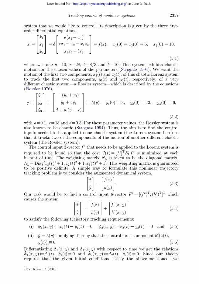
system that we would like to control. Its description is given by the three first-order differential equations,

_xd

_x1

_x2

_x3

264

375Z d

sðx 2K x1Þrx1K x 2K x1x 3

x1x2Kbx3

264

375Z f ðxÞ; x1ð0ÞZ x3ð0ÞZ 5; x 2ð0ÞZ 10;

ð5:1Þwhere we take sZ10, rZ28, bZ8/3 and dZ10. This system exhibits chaoticmotion for the chosen values of the parameters (Strogatz 1994). We want themotion of the first two components, x1(t) and x2(t), of this chaotic Lorenz systemto track the first two components, y1(t) and y2(t), respectively, of a verydifferent chaotic system—a Rossler system—which is described by the equations(Rossler 1976),

_yd

_y1

_y2

_y3

264

375Z

Kðy2 Cy3Þy1 Cay2

dCy3ðy1KcÞ

264

375Z hðyÞ; y1ð0ÞZ 3; y2ð0ÞZ 12; y3ð0ÞZ 6;

ð5:2Þwith aZ0.1, cZ18 and dZ0.3. For these parameter values, the Rossler system isalso known to be chaotic (Strogatz 1994). Thus, the aim is to find the controlinputs needed to be applied to one chaotic system (the Lorenz system here) sothat it tracks two of the components of the motion of another different chaoticsystem (the Rossler system).

The control input 3-vector f c that needs to be applied to the Lorenz system is

required to be found so that the cost Jðt ÞZ ½f c�TNL fc is minimized at each

instant of time. The weighting matrix NL is taken to be the diagonal matrix,NLZDiag½x 3ðt Þ2C1; x2ðt Þ2C1; x1ðt Þ2C1�. This weighting matrix is guaranteedto be positive definite. A simple way to formulate this nonlinear trajectorytracking problem is to consider the augmented dynamical system,

_x

_y

" #Z

f ðxÞhðyÞ

" #: ð5:3Þ

Our task would be to find a control input 6-vector F cZ ½ðf cÞT; ðhcÞT�T whichcauses the system

_x

_y

" #Z

f ðxÞhðyÞ

" #C

f cðx; yÞhcðx; yÞ

" #ð5:4Þ

to satisfy the following trajectory tracking requirements:

ðiÞ f1ðx; yÞdx1ðt ÞK y1ðt ÞZ 0; f2ðx; yÞdx2ðt ÞK y2ðt ÞZ 0 and ð5:5Þ

ðiiÞ _y Z hðyÞ; implying thereby that the control force component hcðxðtÞ;yðt ÞÞh0: ð5:6Þ

Differentiating f1ðx; yÞ and f2ðx; yÞ with respect to time we get the relations_f1ðx; yÞd _x1ðtÞK _y1ðtÞZ0 and _f2ðx; yÞd _x2ðtÞK _y2ðtÞZ0. Since our theoryrequires that the given initial conditions satisfy the above-mentioned two



30

20

10

0

−20

−10

−30firs

t com

pone

nt o

f L

oren

z an

d R

ossl

er s

yste

m

0 10 20 30 40 50time

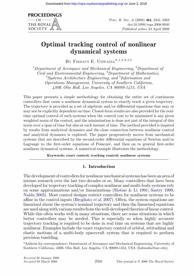
Figure 1. The dynamics of the first component of the Lorenz system x1(t) and the Rossler systemy1(t) are shown by the solid line and the thick dashed line, respectively. Fifty seconds of responseare shown.

F. E. Udwadia2358


trajectory requirements, and they do not, we shall modify the trajectoryrequirements to

_f1 ZKaf1; _f2 ZKaf2; ð5:7Þ

where aO0 is chosen to be a suitable parameter. We note that asymptoticsolutions of equation (5.7) as t/N are fi(t)Z0, iZ1, 2 as required by (5.5). Theparameter a in the numerical example is chosen to be 0.5. The trajectorydescription given by (5.7) and (5.6) then leads to (see equation (4.4))

Ag Z

1 0 0 K1 0 0

0 1 0 0 K1 0

0 0 0 1 0 0

0 0 0 0 1 0

0 0 0 0 0 1

266666664

377777775

and bg Z

Kaðx1K y1ÞKaðx2K y2Þ

hðyÞ

264

375: ð5:8Þ

The weighting matrix N for the augmented six-dimensional dynamical systemgiven in equation (5.4) will also need to be augmented so it is a diagonal 6 by 6matrix. Owing to the trajectory requirement hc(t)h0, we can choose its lastthree diagonal entries to be each equal to unity; the first three diagonal entriesremain the same as those of the matrix NL. The explicit control input that causesthe trajectory described by (5.6) and (5.7) to be tracked is then given by equation(4.14) with BsZAgN

K1=2, since the 6 by 6 matrix Mg is an identity matrix.All the computations are performed using MATLAB and the integration is

carried out using a relative error tolerance of 10K10 and an absolute errortolerance of 10K13. Figure 1 shows the dynamics of the first component of the twoseparate dynamical systems described by equations (5.1) and (5.2).



2.0

1.5

1.0

0.5

0

−0.5

−1.0

−1.5

−2.00 10 20 30

time

trac

king

err

or

40 50

(a)

trac

king

err

or (

×10

–12 )

6

4

2

0

−2

−4

−680 85 90 95 100

time

(b)

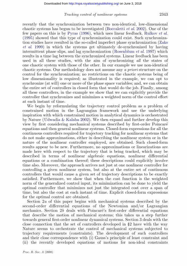
Figure 2. (a) The solid line shows e1(t) over 50 s of integration. The dashed line shows e2(t).(b) Tracking errors e1(t) and e2(t) over the time interval [80–100] seconds using the same lineconventions as in (a).

3

2

1

cont

rol i

nput

s to

Ros

sler

sys

tem

(×1

0−1

1 )

0

−1

−2

0 10 20 30 40 50time

0 10 20 30 40 50time

(a)3

2

1

cont

rol i

nput

s to

Lor

enz

syst

em (

×10

4 )

0

−1

−2

−3

−4

−5

(b)

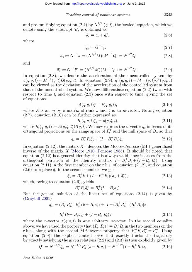
Figure 3. (a) Components of the control inputs acting on the Rossler system. Note that the verticalscale ranges from approximately K3!10K11 to 3!10K11, making hcz0. The first componentof the control input is shown by a solid line, the second by a dashed line and the third by athick solid line. (b) Components of the control inputs acting on the Lorenz system, using the sameline notation.



On application of the optimal control input, the tracking errors e1(t)dx1(t)Ky1(t) and e2(t)dx1(t)Ky1(t) are shown in figure 2. These errors, as timeincreases, go down to the same order of magnitude as the tolerance used in thenumerical integration of the differential equations as shown in figure 2b.

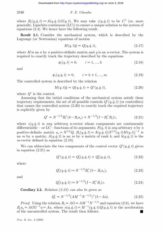
Figure 3a shows the control inputs acting on the Rossler system. They aretheoretically supposed to be zero, as required by the second trajectory require-ment (5.6). They are seen to be very small, and of the same order of magnitude asthe tolerances with which the integration is carried out. Figure 3b shows thecontrol inputs required to be given to the Lorenz system so that it tracks thefirst two components of the Rossler system. The third component of the controlinput to the Lorenz system is seen to be zero, since we require only the first twocomponents to be tracked. The optimal control cost J(t) is shown in figure 4.



10

8

6

4

2

0 10 20 30time

40 50

Figure 4. The optimal control cost JðtÞZ ½Fc�TNðxÞFc as a function of time.

30

20

10

0

−10

−20

−30−30 −20 −10 10 20 300

Figure 5. Projection of phase space trajectories over the time interval [0–100] seconds of thecontrolled Lorenz system (dashed line) on the (x1, x2) plane and those of the Rossler system(solid line) on the (y1, y2) plane.

F. E. Udwadia2360


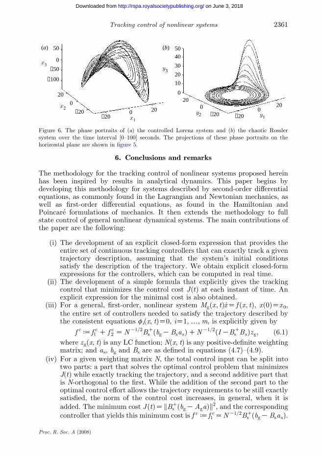
The projection of the phase trajectory of the controlled Lorenz system on tothe (x1, x2) plane (solid line) and the projection of the corresponding phasetrajectory of the Rossler system on to the (y1, y2) plane (dashed line) areshown in figure 5. The figure shows the manner of convergence of theseprojected trajectories, which start with different initial conditions. Because thethird component of the Rossler system is not tracked, the three-dimensionalphase portrait looks very different for the controlled Lorenz system. The phasespace portraits of these two systems are shown in figure 6.



50

0

−50

−100

20

0

0−20−20

20

(a) 5040

30

20

10

020

0−20 −20

020

(b)

3

Figure 6. The phase portraits of (a) the controlled Lorenz system and (b) the chaotic Rosslersystem over the time interval [0–100] seconds. The projections of these phase portraits on thehorizontal plane are shown in figure 5.



6. Conclusions and remarks

The methodology for the tracking control of nonlinear systems proposed hereinhas been inspired by results in analytical dynamics. This paper begins bydeveloping this methodology for systems described by second-order differentialequations, as commonly found in the Lagrangian and Newtonian mechanics, aswell as first-order differential equations, as found in the Hamiltonian andPoincare formulations of mechanics. It then extends the methodology to fullstate control of general nonlinear dynamical systems. The main contributions ofthe paper are the following:

(i) The development of an explicit closed-form expression that provides theentire set of continuous tracking controllers that can exactly track a giventrajectory description, assuming that the system’s initial conditionssatisfy the description of the trajectory. We obtain explicit closed-formexpressions for the controllers, which can be computed in real time.

(ii) The development of a simple formula that explicitly gives the trackingcontrol that minimizes the control cost J(t) at each instant of time. Anexplicit expression for the minimal cost is also obtained.

(iii) For a general, first-order, nonlinear system Mgðx; tÞ _xZ f ðx; tÞ, x(0)Zx0,the entire set of controllers needed to satisfy the trajectory described bythe consistent equations fi(x, t)Z0, iZ1, ., m, is explicitly given by

f cdf c1 C f c2 ZNK1=2BCs ðbgKBsa sÞCNK1=2ðIKBC

s B sÞzg; ð6:1Þwhere zg(x, t) is any LC function; N(x, t) is any positive-definite weightingmatrix; and as, bg and Bs are as defined in equations (4.7)–(4.9).

(iv) For a given weighting matrix N, the total control input can be split intotwo parts: a part that solves the optimal control problem that minimizesJ(t) while exactly tracking the trajectory, and a second additive part thatis N-orthogonal to the first. While the addition of the second part to theoptimal control effort allows the trajectory requirements to be still exactlysatisfied, the norm of the control cost increases, in general, when it isadded. The minimum cost JðtÞZkBC

s ðbgKAgaÞk2, and the correspondingcontroller that yields this minimum cost is f cdf c1 ZNK1=2BC

s ðbgKBsa sÞ.



F. E. Udwadia2362


The addition of the second part f c2 ZNK1=2ðIKBCs BsÞzg, so that f cd

f c1 C f c2 , increases the cost beyond the optimal by kðIKBCs BsÞzgk2. At

each instant of time t, when zg(x, t) belongs to the range space of BTs ,

f c2 ðt ÞZ0, so that f cðt Þdf c1 ðtÞ, hence making the control at that instantof time optimal.

(v) The close connection between nonlinear control and analytical mechanics ispointed out. Here we see that Nature seems to control a mechanical systemso that it satisfies a given set of trajectory requirements—or alternativelystated, tracks a given trajectory—by using feedback control, much like acontrol engineer, except that instead of proportional, integral or derivativefeedback control, which is commonly used by the control engineer, it usesacceleration feedback. While considerable work has been done on PIDcontrol, acceleration feedback seems to be far less studied by modern-daycontrol engineers. Following Nature’s cue, the results developed in thispaper point perhaps towards the need for more work in the area ofacceleration feedback inmechanical systems. Furthermore,Nature seems tominimize the control cost JðtÞZ ½Qc�TNQc at each instant of time, and itappears to useMK1ðq; tÞ for the weighting matrixN. Nature’s choice of thisweighting matrix can be understood when thought of in terms of a multi-body mechanical system that is required to satisfy a given trajectorydescription (a set of constraints), and so track a given trajectory. Since ittakes a larger control effort to move a body belonging to the multi-bodysystem that has a larger inertia, Nature, in its effort to make the entiresystem satisfy the given trajectory description, appears to preferapplying control forces to bodies with the smaller inertias. Again, followingNature’s cue, the use of MK1ðq; tÞ as a weighting matrix for defining thecontrol cost may be useful in many other dynamical systems, especiallymechanical ones.

(vi) While we have demonstrated the methodology by illustrating its use indetermining the control required to be applied to a chaotic Lorenz system sothat it tracks some components of the motion of another chaotic Rosslersystem, the general methodology can be used for more complex nonlinearmechanical systems dealingwith, for example, orbitalmechanics (Lam2006).

(vii) Finally, we note that the methodology presented herein does not include anymagnitudeconstraintsonthecontrol, andworkonthis topic is currentlybeingpursued. Furthermore, the results provided herein deal with full state controland further developments along the lines pursued herein to underactuatedrobotic systems would be useful. The effects of model errors and disturbancecontrol also need to be investigated.

References

Boccaletti, S., Kurths, J., Osipov, G., Valladares, D. & Zhou, C. 2002 The synchronization ofchaotic oscillators. Phys. Rep. 366, 1–101. (doi:10.1016/S0370-1573(02)00137-0)

Brockett, R. W. 1977 Control theory and analytical mechanics. In Geometric control theory (edsC. Martin & R. Herman), pp. 1–66. Brookline, MA: Math. Sci. Press.

Brogliato, B., Lozano, R. & Maschke, B. 2007 Dissipative systems analysis and control. Berlin,Germany: Springer.


http://dx.doi.org/doi:10.1016/S0370-1573(02)00137-0




Chaou, Y. & Chang, W. 2004 Trajectory control. Lecture Notes on Control and InformationSciences. Berlin, Germany: Springer.

Chen, H. K. 2002 Chaos and synchronization of a symmetric gryo with linear plus cubic damping.J. Sound Vib. 255, 719–740. (doi:10.1006/jsvi.2001.4186)

Gauss, C. F. 1829 Uber ein neues algemeines Grundgesetz der Mechanik. Zeitschrift fur die Reineund Angewandte Mathematik 4, 232–235.

Goldstein, H. 1976 Classical mechanics. New York, NY: Addison-Wesley.Graybill, F. 2001 Matrices with application to statistics Duxbury classics series. Pacific Grove, CA:

Duxbury Publishing Company.Hamel, G. 1949 Theoretische mechanik. Berlin, Germany: Springer.Lagrange, J. L. 1811 Mechanique analytique. Paris, France: Mme Ve Coureier.Lam, T. 2006 New approach to mission design based on the fundamental equation of motion.

J. Aerosp. Eng. 19, 59–67. (doi:10.1061/(ASCE)0893-1321(2006)19:2(59))Lei, Y., Xu, W. & Zheng, H. 2005 Synchronization of two chaotic gyros using active control. Phys.

Lett. A 343, 153–158. (doi:10.1016/j.physleta.2005.06.020)Moore, E. H. 1910 On the reciprocal of the general algebraic matrix. Abstr. Bull. Am. Soc. 26,

394–395.Naidu, D. 2003 Optimal control systems. London, UK: CRC Press.Penrose, R. 1955 A generalized inverse of matrices. Proc. Camb. Philos. Soc. 51, 406–413.Poincare, H. 1901 Sur une forme nouvelle des equations de la mechanique. CR Acad. Sci. Paris

132, 369–371.Pyras, K. 1996 Weak and strong synchronization of chaos. Phys. Rev. E 54, 4508–4511. (doi:10.

1103/PhysRevE.54.R4508)Rosenblum, M., Pilkovsky, A. & Kruths, J. 1997 From phase to lag synchronization in coupled

chaotic oscillators. Phys. Rev. Lett. 78, 4193–4196. (doi:10.1103/PhysRevLett.78.4193)Rossler, O. 1976 An equation for continuous chaos. Phys. Lett. A 57, 397–398. (doi:10.1016/0375-

9601(76)90101-8)Rulkov, N., Sushchik,M., Tsimring, L. &Abarbanel, H. 1995Generalized synchronization of chaos in

directionally coupled chaotic systems. Phys. Rev. E 51, 980–994. (doi:10.1103/PhysRevE.51.980)Sadegh, N. 1990 Stability analysis of a class of adaptive controllers for robotic manipulators. Int.

J. Robot. 9, 74–92. (doi:10.1177/027836499000900305)Sastry, S. 1999 Nonlinear systems analysis, stability, and control. Berlin, Germany: Springer.Slotine, J. & Li, W. 1991 Applied nonlinear control. New York, NY: Englewood Cliffs.Strogatz, S. 1994 Nonlinear dynamics and chaos. Boulder, CO: Westview Press.Udwadia, F. E. 2000 Fundamental principles of lagrangian dynamics: mechanical systems with

non-ideal, holonomic, and non-holonomic constraints. J. Math. Anal. Appl. 252, 341–355.(doi:10.1006/jmaa.2000.7050)

Udwadia, F. E. & Kalaba, R. E. 1992 A new perspective on constrained motion. Proc. R. Soc. A439, 407–410. (doi:10.1098/rspa.1992.0158)

Udwadia, F. E. & Kalaba, R. E. 1996 Analytical dynamics: a new approach. Cambridge, UK:Cambridge University Press.

Udwadia, F. E. & Kalaba, R. E. 2002 On the foundations of analytical dynamics. Int. J. Nonlin.Mech. 37, 1079–1090. (doi:10.1016/S0020-7462(01)00033-6)

Udwadia, F. E. & Phohomsiri, P. 2007 Explicit Poincare equations of motion for generalconstrained systems. Part I. Analytical results. Proc. R. Soc. A 1825, 1–14. (doi:10.1098/rspa.2007.1825)

Zaks, A., Park, E.-H., Rosenblum, M. & Kruths, J. 1999 Alternating locking ratios in imperfectphase synchronization. Phys. Rev. Lett. 82, 4228–4231. (doi:10.1103/PhysRevLett.82.4228)


http://dx.doi.org/doi:10.1006/jsvi.2001.4186

http://dx.doi.org/doi:10.1061/(ASCE)0893-1321(2006)19:2(59)

http://dx.doi.org/doi:10.1061/(ASCE)0893-1321(2006)19:2(59)

http://dx.doi.org/doi:10.1016/j.physleta.2005.06.020

http://dx.doi.org/doi:10.1103/PhysRevE.54.R4508

http://dx.doi.org/doi:10.1103/PhysRevE.54.R4508

http://dx.doi.org/doi:10.1103/PhysRevLett.78.4193

http://dx.doi.org/doi:10.1016/0375-9601(76)90101-8

http://dx.doi.org/doi:10.1016/0375-9601(76)90101-8

http://dx.doi.org/doi:10.1103/PhysRevE.51.980

http://dx.doi.org/doi:10.1177/027836499000900305

http://dx.doi.org/doi:10.1006/jmaa.2000.7050

http://dx.doi.org/doi:10.1098/rspa.1992.0158

http://dx.doi.org/doi:10.1016/S0020-7462(01)00033-6



http://dx.doi.org/doi:10.1103/PhysRevLett.82.4228


optimal tracking control of nonlinear dynamical...

Documents